Embed Size (px)
Citation preview

Topics in the Modeling, Analysis, and Optimisation ofSignalised Road Intersections
A Project Report
Submitted in partial fulfilment of the
requirements for the Degree of
Master of Engineering
in
Telecommunications
by
Pramod MJ
under the guidance of
Prof. Anurag Kumar
Electrical Communication Engineering
Indian Institute of Science
BANGALORE – 560 012
June 2013

Abstract
A network of roads carries vehicular traffic, and to a communication network engineer it would
look similar to a packet network. Long stretches of roads would seem similar to communica-
tion links, whereas signalised intersections would appear similar to packet switching devices.
Indeed, for several decades, traffic engineers have brought to bear congestion theory (stochastic
and deterministic) to model and analyse the flow of traffic on roads. With the possibility of
Intelligent Transportation Systems (ITS) becoming a reality in the not too distant future, in-
creasing attention is now being paid to the modeling, analysis, inference, and control of traffic
in road networks.
With this background in mind, in this thesis we first revisit the problem of congestion modeling
at a signalised traffic intersection. An incoming road at such an intersection can be viewed as a
queue with an interrupted server. Due to car following behaviour, a special feature in the case
of road traffic is that the clearance times of successive vehicles at an intersection are dependent.
With this in mind, our first aim in the work reported here has been to develop an approximation
for the expected delay of vehicles at a segment of road served by a traffic light, where we assume
a Semi Markov (SM) car-following model. Assuming a Poisson arrival process of a mix of
vehicles, we call this an interrupted M/SM/1 queue. The interrupted M/G/1 (more precisely,
the interrupted M/GI/1 queue) has been well studied. Also, in the traffic engineering literature
there is a popular approximation for the mean delay in an interrupted M/D/1 queue, i.e., the
Webster formula. We use the analysis of Sengupta [17] to (i) develop an understanding of the
various terms in Webster’s formula, and (ii) develop extensions of this formula to the M/G/1
and M/SM/1 interrupted queues. The quality of the approximations is illustrated by several
i
ii
numerical examples.
We also complement the above work with optimisation of signal timing, a study of tandem
intersections, and a study of the effect of batching due the behaviour of two wheelers in typical
Indian traffic conditions.

Acknowledgement
I would like to offer my special thanks to all those who provided me the possibility to complete
this thesis.
I owe my deepest gratitude to Prof. Anurag Kumar. I would like to thank him for the guidance
he provided me thoughout this work. He has been an inspiration not just in my academic life. I
also thank him for the patience he showed while helping during the writing of this thesis.
I thank my parents for their blessings and unwavering support.
I would like to thank my friends (there are too many of them, for me to name here), especially
Ashok Krishnan, for the help and support they provided during the completion of this work.
iii

Contents
1 Introduction 1
2 Literature Survey 4
3 Modeling the Queues at a Traffic Intersection 11
3.1 Queueing and Service at a Traffic Intersection . . . . . . . . . . . . . . . . . . 12
3.1.1 Arrival Process Model . . . . . . . . . . . . . . . . . . . . . . . . . . 14
3.1.2 Service Model . . . . . . . . . . . . . . . . . . . . . . . . . . . . . . 15
3.2 Relation to the PCU terminology: . . . . . . . . . . . . . . . . . . . . . . . . 22
3.3 Traffic Intersection Simulation . . . . . . . . . . . . . . . . . . . . . . . . . . 24
3.4 Example Traffic Models . . . . . . . . . . . . . . . . . . . . . . . . . . . . . 26
3.5 Preemptive service vs. nonpreemptive service . . . . . . . . . . . . . . . . . . 28
3.6 Service of the First Arrival in a Busy Period . . . . . . . . . . . . . . . . . . . 30
3.7 Stability Criterion . . . . . . . . . . . . . . . . . . . . . . . . . . . . . . . . . 33
4 Analysis of Queues at Traffic Intersections 35
4.1 Mean Delay Analysis - Preliminaries . . . . . . . . . . . . . . . . . . . . . . . 36
iv

CONTENTS v
4.2 The Analysis in Sengupta [17] . . . . . . . . . . . . . . . . . . . . . . . . . . 39
4.2.1 Mean Work in the System . . . . . . . . . . . . . . . . . . . . . . . . 40
4.2.2 Mean Waiting Time . . . . . . . . . . . . . . . . . . . . . . . . . . . 42
4.2.3 Approximations for Mean Delay . . . . . . . . . . . . . . . . . . . . . 44
4.2.4 Numerical Comparison Between Various Approximations . . . . . . . 46
4.2.5 Comparison between the Approximation [4.19] and Simulation . . . . 51
4.3 Webster’s Approximation . . . . . . . . . . . . . . . . . . . . . . . . . . . . . 55
4.3.1 What is Webster’s Formula Approximating? . . . . . . . . . . . . . . . 57
5 Understanding and Extending Webster’s Formula 61
5.1 Understanding Webster’s Approximation . . . . . . . . . . . . . . . . . . . . . 61
5.2 Extending Webster’s Approximation to M/G/1 and M/SM/1 models . . . . . . 65
5.2.1 Extending Webster’s Approximation to M/G/1 model . . . . . . . . . . 65
5.2.2 Extending Webster’s Approximation to M/SM/1 model . . . . . . . . . 66
5.3 Numerical Study of Extensions of Webster’s model . . . . . . . . . . . . . . . 68
5.4 Variants of Webster’s Approximation . . . . . . . . . . . . . . . . . . . . . . . 72
5.4.1 Webster Variant I : Modified first term and correction term . . . . . . . 72
5.5 Conclusion . . . . . . . . . . . . . . . . . . . . . . . . . . . . . . . . . . . . 76
6 Optimisation of Signal Timings 77
7 Tandem Queues 80
8 Extending Modeling and Analysis to Motorcycle Traffic 86
CONTENTS vi
8.1 Motorcycles at a Signalized intersection . . . . . . . . . . . . . . . . . . . . . 86
8.2 Analysis of Queues containing Motorcycles at a Signalized intersection . . . . 89
9 Future Work 102
Bibliography 103
Chapter 1
Introduction
An Intelligent Transportation System (ITS) refers to the use of measurement, modeling, infer-
ence, and control techniques for the management of road networks. Examples of ITS appli-
cations would be: passenger information systems for a city bus service, on-line optimisation
of traffic signal timing for traffic flow management, and decision support system for situation
management following a road blockage due to an accident or breakdown. Thus, with ITS in
mind, in this thesis we report our study of analytical modeling of congestion at a signalised
traffic intersection. While this is a classical topic [[10, 11, 12, 21]], it is the first topic that
would be undertaken in any research effort on modeling of road networks. Further, even this
classical topic could do with some additional research in removing some of the simplifications
in earlier models, and in developing new models for the peculiar traffic conditions that exist in
developing countries, such as India.
An intersection is a junction where two or more roads cross, and is generally controlled by traffic
signals. The congestion phenomenon at an intersection is governed by parameters such as the
durations of the red and green periods, the arrival rates of the vehicles, and the rate at which
vehicles can exit the intersection during the green time. An understanding of such congestion
phenomena, and the design of signal timing as to optimise the delay at an intersection, are basic
questions in any road network analysis and design.
1
CHAPTER 1. INTRODUCTION 2
The road network bears close resemblance to a packet network with the long stretches of roads
and the intersections being similar, respectively, to the communication links and the packet
switches. If we consider a signalised intersection with 4 stretches of roads bringing traffic to the
intersection, then with the assumption that free left turns are not allowed, we can consider them
each to be a queue with interrupted service. In an interrupted queue the server performs service
for a random duration of time and then remains idle for a random duration of time. This cycle
continues irrespective of whether the queue is empty or not. This provides the motivation to use
queuing models to analyse a signalised intersection. We will look at some of the currently used
analytical models for analysing various models of traffic at an intersection. The approximation
by Webster is the most commonly used one, though we will find that it only models the deter-
ministic service model. We will then suggest improved approximations for all the models that
we will be studying.
Keeping in mind the car-following behavior, we model the service process as a Semi-Markov
(SM) model. We will also be looking at simplified service models derived from the SM mod-
els, such as the deterministic model, where all the vehicles are assumed to take the same service
time, which would be the mean service time calculated over all types of vehicles in the network;
the general independent model, where the service times of successive vehicles are independent
and are drawn from a general distribution. We study analytical models which provides ap-
proximations for the mean delay estimation problem. The quality of the approximations are
illustrated by comparing them with the simulation results. Extensions of Webster’s formula are
suggested, which provides good approximations M/G/1 and M/SM/1 interrupted queue models
at signalised intersections. Optimisation of signal timings are done for M/D/1 and M/G/1 mod-
els using the approximations for mean delay. We further proceed to estimate the mean delay at
a two-stage tandem queue, where both the intersections are assumed to be M/D/1 interrupted
queues. Given that in developing countries such as India, 2 wheelers, which are prone to batch-
ing with larger vehicles while waiting at the intersection, form the bulk of the traffic, we study
at the effect of batching in typical Indian traffic conditions. In Chapter [2] we discuss in detail
the various existing models available for road networks. In Chapter [3] we discuss about mod-
CHAPTER 1. INTRODUCTION 3
eling different aspects of traffic at a signalized intersection. In Chapter [4] different analytical
models are considered which provide good approximations for the model that we are study-
ing. In Section [5.3] we compare Webster’s formula and its extensions with the simulations
of models that we considered in the Chapter [3] and find out the analytical model that gives
the best approximation for each of the service models that we have considered. In Chapter [6]
an optimisation problem where the signal timings are optimised to minimize the mean delay
at the intersection, is studied, for M/D/1 and M/G/1 interrupted queue models. In Chapter [8]
we study the effects of batching due to 2-wheeler traffic on typical Indian traffic conditions. In
Chapter [7] we study a 2-stage tandem queue where the first intersection is assumed to be M/D/1
interrupted queue and the second intersection has a deterministic service process, to estimate
the mean delay across the tandem queue.

Chapter 2
Literature Survey
Though the problem discussed might be the same, the traffic engineers and the queueing (net-
working) researchers use different terminology to describe similar parameters in the problem.
Here we look to bring a consensus between the terminologies used by the traffic engineers and
the queueing (networking) researchers and explain what they means. Individual parameters of
the pairs given below are viewed as the same under our problem setting.
1. Flow rate - Arrival rate : According to traffic engineers, flow rate gives the number of
vehicles passing through a given point on the road in unit time. This could in turn be
viewed as the rate at which vehicles arrive into an intersection. According to queueing
researchers, arrival rate gives the rate at which packets arrive into a queue.
2. Capacity - Service rate : To traffic engineers, capacity gives the maximum number of
vehicles per unit time, which can be accommodated under any given conditions. Service
rate , according to queueing researchers, means the number of packets serviced per unit
time (or the rate at which the queues are drained) by the whole system.
Capacity is defined as the maximum number of vehicles per unit time, which can be
accommodated under any given conditions. But there is a question of how best to define
a vehicle when the traffic is heterogenous, i.e., contains different types of vehicle. This
makes it necessary to have a standard unit for vehicles. Thus to deal with heterogenous
4

CHAPTER 2. LITERATURE SURVEY 5
traffic, each vehicle type is converted into its PCU (Passenger Car Units) values. The
PCU is the universally adopted unit of measurement of traffic volume, defined by taking
the passenger car as the standard vehicle. The passenger car has a PCU value equal to 1
and PCU values of other vehicles are calculated considering their service times in relation
to that of a passenger car.
3. Degree of Saturation - Server Utilization : In traffic engineering terms, degree of satu-
ration is defined as the ratio of flow to capacity. In queueing theory terms, server utiliza-
tion is defined as the ratio of mean arrival rate to mean service rate.
The problem of estimating mean delay at fixed-cycle (green time and red time durations are
deterministic) traffic lights has been well studied in traffic engineering. The earliest models
considered had vehicles arriving at regularly spaced intervals and service of vehicles happening
at regularly spaced intervals (deterministic) [2]. Webster [21] assumes Poisson arrival of vehi-
cles and deterministic service times to model the fixed-cycle traffic light problem. Webster’s
formula is the most famous result for this specific problem.
We see that Poisson point process is one of the most widely used traffic flow models [18][13].
The main attraction for this model is that it is mathematically tractable. It is a reasonable model
when the traffic density is light. Poisson point process assumes that successive gaps between
vehicles are independent. The use of Poisson point process for arrivals is justified, because in
the roads leading upto the intersections the vehicles will never be closely packed and will leave
sufficient distance between each other. Thus it is reasonable to think of vehicles as points, in
roads leading up to the intersection.
Webster arrived at his formula empirically using simulations. Many attempts have been made
to come up with a complete analytic solution. McNeil [10] shows that the problem of obtaining
an exact formula for mean delay can be reduced to that of obtaining an exact formula for the
mean overflow queue length (mean stationary queue length at the end of green time). Darroch
[4] suggests a method to compute the mean overflow queue length exactly, but provided a com-
putationally complex approach. McNeil [10], Miller [11] and Newell [12] give approximate

CHAPTER 2. LITERATURE SURVEY 6
formulas for computing the mean overflow queue lengths. Another thing to notice is, almost all
of these works except Newell assumes the service times to be deterministic, where as Newell
assumes a general service time distribution. Ohno [13] compares the works of Webster, Mc-
Neill, Miller and Newell, and concludes that the delays estimated by them are extremely similar
for Poisson arrivals.
Since in this work our main focus is to extend the problem of estimating mean delay at fixed-
cyle traffic lights to general service distribution and semi-Markov service distributions, we will
focus on Webster’s model and will look to extend it to these service models. Therefore, we will
assume Poisson arrival process as well in our work.
The semi-Markov service process tells that the service time of a customer is dependent on the
current customer and the customer it follows. How this transforms into the traffic engineering
domain is explained by the car following models. Car following is the task of one vehicle
following an another [15]. The task of driving a vehicle behind another is further subdivided
into 3 tasks.
1. Perception : The information gathered through the visual channel.eg: inter-vehicle spac-
ing, relative velocity.
2. Decision Making : The driver has to interpret the informations gathered through visual
senses and then make a decision as to accelerate or brake or something else.
3. Control : Factors related to the skill of the driver.
While following another vehicle, the current vehicle would want to move at particular speed
ensuring a safe tail-to-tail distance with the preceding vehicle. Rothery [15] gives a model to
relate the speed of the vehicle (V ) and tail-to-tail distance between vehicles (D),
D = α + βV + γV 2 (2.1)
where the physical interpretation of the parameters can be given as,

CHAPTER 2. LITERATURE SURVEY 7
α = the effective vehicle length, L
β = the reaction time
γ = the reciprocal of twice the maximum average deceleration of a following vehicle
Maitra-etal [8] discusses the relation between speed of vehicles and the flow rate. They quantify
congestion on road for any given operating condition, using the speed-flow graph. They shows
that, as velocity increases flow rate of vehicles also increases and hits a maximum value and
then decreases with further increase in speed. We can also explain this as the variation of head-
to-head distance between vehicles w.r.t to speed by the well known relation between flow rate
(λ), speed (v) and tail-to-tail distance between vehicles (D(v)) given by the expression [2.1].
λ = v
D(v)
May[9] gives a detailed account of various models of Car following theories. Pioneering works
in this field were done by Pipes, Forbes, and the General Motors researchers.
1. Pipes’ Theory : Pipes characterized the motion of vehicles according to the California
Motor Vehicle Code, namely : “A good rule for following another vehicle at a safe dis-
tance is to allow yourself at least the length of a car between your vehicle and the vehicle
ahead for every ten miles per hour of speed at which you are travelling”. According to
Pipes’ car following theory, the minimum safe headway increases linearly with speed.
2. Forbes’ Theory : Forbes characterized the car following behavior by considering the
reaction time needed for the following vehicle to perceive the need to decelerate and then
apply the brakes. This means that the gap between rear of the lead vehicle and the front
of the following vehicle must be greater than or at least equal to the reaction time. Thus
Forbes define the minimum time headway as equal to the sum of reaction time (minimum
time gap) and the time required for the lead vehicle to traverse a distance equal to its
length. Here also the minimum safe distance headway increases lineraly with speed.
CHAPTER 2. LITERATURE SURVEY 8
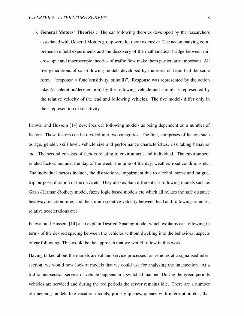
3. General Motors’ Theories : The car following theories developed by the researchers
associated with General Motors group were lot more extensive. The accompanying com-
prehensive field experiments and the discovery of the mathematical bridge between mi-
croscopic and macroscopic theories of traffic flow make them particularly important. All
five generations of car-following models developed by the research team had the same
form , “response = func(sensitivity, stimuli)”. Response was represented by the action
taken(acceleration/deceleration) by the following vehicle and stimuli is represented by
the relative velocity of the lead and following vehicles. The five models differ only in
their represention of sensitivity.
Panwai and Hussein [14] describes car following models as being dependent on a number of
factors. These factors can be divided into two categories. The first, comprises of factors such
as age, gender, skill level, vehicle size and performance characteristics, risk taking behavior
etc. The second consists of factors relating to environment and individual. The environment
related factors include, the day of the week, the time of the day, weather, road conditions etc.
The individual factors include, the distractions, impairment due to alcohol, stress and fatigue,
trip purpose, duration of the drive etc. They also explain different car following models such as
Gazis-Herman-Rothery model, fuzzy logic based models etc which all relates the safe distance
headway, reaction time, and the stimuli (relative velocity between lead and following vehicles,
relative accelerations etc).
Panwai and Hussein [14] also explain Desired-Spacing model which explains car following in
terms of the desired spacing between the vehicles without dwelling into the behavioral aspects
of car following. This would be the approach that we would follow in this work.
Having talked about the models arrival and service processes for vehicles at a signalised inter-
section, we would now look at models that we could use for analysing the intersection. At a
traffic intersection service of vehicle happens in a switched manner. During the green periods
vehicles are serviced and during the red periods the server remains idle. There are a number
of queueing models like vacation models, priority queues, queues with interruption etc., that
CHAPTER 2. LITERATURE SURVEY 9
behave in a similar way.
In the vacation model, once the busy period is over, the server takes a vacation or a break for
a random amount of time. Once the vacation is over, it will check the queue again and if it is
empty, it will either wait for a customer to come or will take another vacation depending on
whether it is a single vacation or multiple vacation model. But this model is not used, as this
does not realistically represent the traffic at intersection, as in an intersection the server could
take a break even in the middle of service.
In queues with interruption, the queue remains ON for a random length of time, and then turns
OFF for another random length of time. This cycle continues. The queue is serviced only
during the ON times. This model is quite similar to how the traffic works at intersections. The
traffic light for a lane stays green for sometime, and then turns red. This cycle continues. The
vehicles are allowed to cross the intersection only during the green times. Thus the queues with
interruption seems to be a quite reasonable model for studying traffic at an intersection.
Federgruen and Green [5] analyses queues with interruption, with Poisson arrival process and
general i.i.d. service time distributions. The case that Federgruen and Green analyses, where
the arrival rate is same during both ON times and OFF times, and the service time distributions
are same for vehicles arriving during both ON and OFF times, is a special case of the general
model that Sengupta analyses.
Sengupta [17] analyses queues with interruption that are quite general. The arrival rate of vehi-
cles could be different during ON times and OFF times. Similarly the service time distribution
for vehicles arriving during ON times and OFF times can also be different. Sengupta analyses
the model using the concept of residual service times while Federgruen and Green analyses it
using the concept of completion times. We will be following Sengupta’s analysis in this work.
We will take a detailed look at this model in Section [4.2]
In this work we aim to model the intersection with fixed-cycle traffic lights, as a queue with
service interruption and analyse this model to estimate the mean delay at the intersection. We
further aim to extend the Webster’s formula for mean delay estimation, to general and semi-

CHAPTER 2. LITERATURE SURVEY 10
Markov service models. Webster’s formula and its extension to M/G/1 model is used to optimise
the signal timings. We proceed to study the effects of batching which is typical of 2-wheeler
traffic and will attempt to develop an analytical model for estimating the mean delay for traffic
containing 2-wheelers. We then study a 2-stage Tandem queue where the first intersection
is assumed to be a M/D/1 interrupted queue and the second intersection is assumed to have a
deterministic service process, with the aim of obtaining an approximation for mean delay across
the two intersections.
Chapter 3
Modeling the Queues at a Traffic
Intersection
Traffic lights are used to control traffic at intersections. Arriving vehicles queue up during the
red periods of the traffic light that controls their desired exit point, and are allowed to proceed
to their exit point when the light turns green. Typically, the lights are scheduled cyclically, i.e.,
there is a repetitive pattern comprising a cycle time during which there is a fixed pattern of red
and green periods for each light. Given this pattern, the congestion process at the intersection
is governed by arrival processes of vehicles from each road leading into the intersection, and
the driver behaviour when they queue up (e.g., motorcycle drivers might try to jockey their way
into the spaces between four-wheeled vehicles), and the driver behaviour when they exit during
a green time (e.g., a small car following a bus might allow a large tail-to-head distance before
starting to move, as opposed to if the small car is behind another small car). It is this latter
feature of traffic lights that makes the system essentially different from a packet switch in a
packet network. Packets have no "behaviour" of their own, and the centralised scheduling and
routing algorithm, running in the packet switch processor, has complete control over the way
the various packet buffers are served.
11
CHAPTER 3. MODELING THE QUEUES AT A TRAFFIC INTERSECTION 12
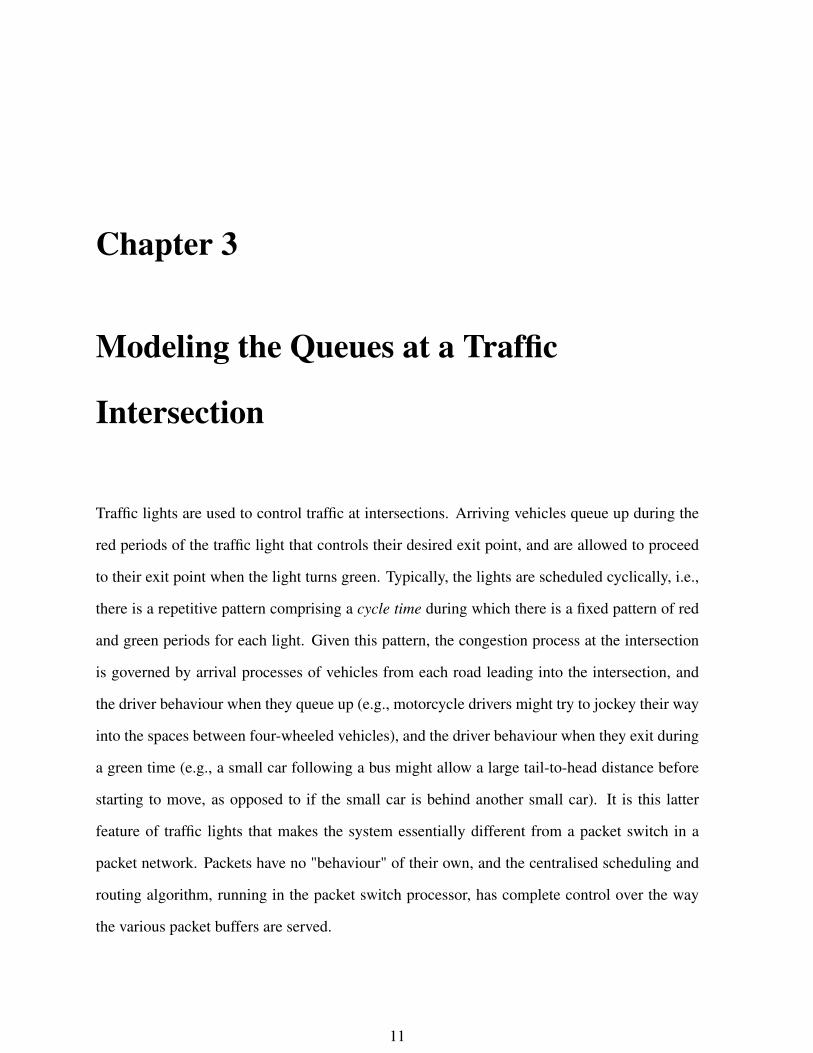
3.1 Queueing and Service at a Traffic Intersection
Figure 3.1: A typical signalised intersection
The figure [3.1] represents a typical signalised intersection, with the traffic signal controlling
the traffic flow through the 4connected roads. Assuming that no free left turns are allowed at
the intersection, we can analyse each road individually and independent of the other roads.
CHAPTER 3. MODELING THE QUEUES AT A TRAFFIC INTERSECTION 13
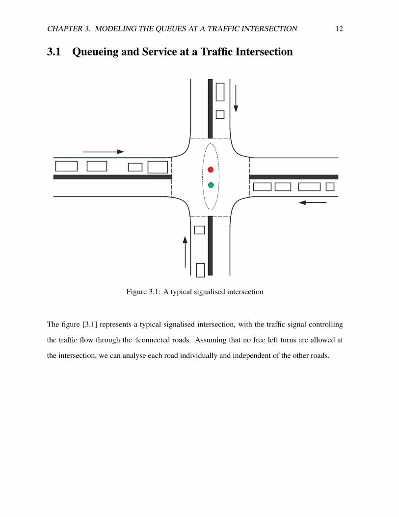
Figure 3.2: A single lane road controlled by a traffic signal
Consider a single lane road leading to an intersection. Assume that the stretch of road that
leads to the intersection is long enough so that the vehicles are cruising before it enters the
intersection. When the lights are red the vehicles arriving are queued one behind the other.
When the lights turn green, the waiting vehicles are serviced (exit) in a first come first served
manner. Clearly, this behaviour is typical of a queue with interrupted service. Hence we model
the single lane traffic controlled by traffic lights as a queue with interrupted service. We will
also make the assumption that one cycle time for the traffic lights comprises of one green time
and one red time.

CHAPTER 3. MODELING THE QUEUES AT A TRAFFIC INTERSECTION 14
Figure 3.3: A queue with interrupted service
In this section we will explain the arrival process model and the service process model that we
will be using in this work.
3.1.1 Arrival Process Model
We have already seen in the literaure survey [2] that the Poisson model is a reasonable model
to use for modelling the arrival process [18][11, 13]. The model has the advantage that it is
mathematically tractable. Most of the researchers, like Webster [21], use the Poisson model for
the arrival process of vehicles into a traffic intersection. The assumption that successive gaps
between vehicles are exponentially distributed and independent is reasonable on the stretch of
road that leads to the traffic intersection, because the vehicles are sufficiently apart from each
other and it is reasonable to think of them as point entities. So we will also assume the arrival
process of vehicles into the intersection to be Poisson.

CHAPTER 3. MODELING THE QUEUES AT A TRAFFIC INTERSECTION 15
3.1.2 Service Model
Notation
λ arrival rate (vehicles/second)
c cycle duration (seconds): one green time + one red time (This is an assumption; in
some cases, during a cycle the same lane may get a green twice.)
g green time duration (seconds)
r red time duration (seconds)
dij minimum distance (meters) from the tail of vehicle i, to the tail of vehicle j. i.e., the
minimum lagging headway required for vehicle j when it is preceded by vehicle
type i, before vehicle j starts moving. We call this minimum lagging headway as
the lagging headway for a vehicle in our service model.
vs speed with which vehicles leave the intersection; in practice, the vehicles would
have to accelerate to reach this speed, but in our analysis we neglect the accelera-
tion time, i.e., we assume that the vehicle accelerates instantly to the exit velocity
vs[[11]]
tijdijvs
li length of vehicle type i
gij distance left by vehicle type j in front of it , when the vehicle in front is of type i,
while waiting in the queue
CHAPTER 3. MODELING THE QUEUES AT A TRAFFIC INTERSECTION 16
HOL Position
Vehicle 1Vehicle 2
Lagging Headway
for vehicle type 2,
d12
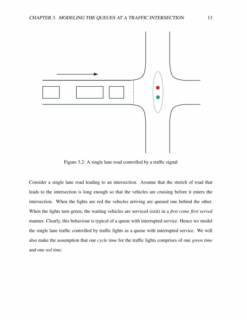
Figure 3.4: Lagging Headway for a vehicle type 2
Now that we have fixed on a model for the arrival process, we need to identify a model that
fits the service process. Due to the car-following behaviour, when vehicles exit a signalized
intersection the headway they have depends both on their own type and the type of vehicle that
it follows (the preceding vehicle). This means that the lagging headway [16] of a particular
vehicle depends both on itself and the preceding vehicle.
In order to develop a queueing analysis, we need to specify a model for the service times re-
quired by the successive vehicles.

CHAPTER 3. MODELING THE QUEUES AT A TRAFFIC INTERSECTION 17
HOL Position
Vehicle 1Vehicle 2Vehicle 3Vehicle 4
l4
g12g23g34
l3 l2 l1
(a) The vehicles lined up waiting at an intersection. The length of the vehicles (li)are marked.
HOL Position
Vehicle 1Vehicle 2Vehicle 3Vehicle 4
l1l2l3l4
g34
d12
g23 g12
(b) The vehicles, once the light has turned green, would start to move. Vehicle 1 isthe first to move. Vehicle 2 starts to move once its tail-to-tail distance with Vehiclel is d12.
HOL Position
Vehicle 1Vehicle 2Vehicle 3Vehicle 4
l1l2l3l4
g12g23g34
d12d23
(c) Vehicle 3 starts to move once its tail-to-tail distance with Vehicle 2 is d23.
HOL Position
Vehicle 1Vehicle 2Vehicle 3Vehicle 4
l1l2l3l4
g12g23g34
d12d23d34
(d) Vehicle 4 starts to move once its tail-to-tail distance with Vehicle 3 is d34.
Figure 3.5: Vehicle following at an signalized intersection
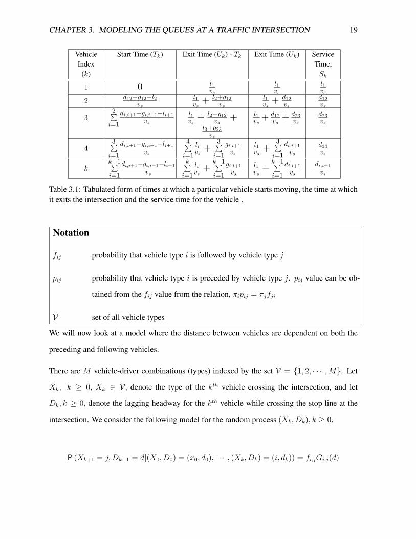
A vehicle is said to have entered service once the preceding vehicle’s tail has crossed the stop
line at the intersection. The service time for a vehicle is the time taken by it to leave the
intersection (i.e., its tail has crossed the stop line) after it has entered service. For a given
constant exit speed, the service time for a vehicle depends on the lagging headway of the vehicle.

CHAPTER 3. MODELING THE QUEUES AT A TRAFFIC INTERSECTION 18
We will derive the service time of a vehicle from this model that we have considered.
Consider that light turned green at time t = 0. A vehicle starts moving when there is enough
head room between itself and the preceding vehicle (i.e., minimum required lagging headway−length
of the vehicle). For a vehicle to exit the intersection, its tail has to cross the stop line. Service
time of a vehicle is difference of its exit time and exit time of the previous vehicle that entered
service.
Let Uk represent the exit time of kthvehicle from the intersection. Then for k ≥2 ,
Uk =k−1∑i=1
di,i+1 − gi,i+1 − li+1
vs+
k∑i=1
livs
+k−1∑i=1
gi,i+1
vs
where the first term represents the time at which kth vehicle starts to move, and the second and
third terms represent the time taken by the kth vehicle to exit the intersection once it has started
moving.
The service time for kth vehicle is the time taken to cross the stop line, after the preceding
vehicle has crossed the stop line. Hence the service time for the kth vehicle, Sk, can be expressed
as,
Sk =Uk − Uk−1
=dk−1,k − gk−1,k − lkvs
+ lkvs
+ gk−1,k
vs
=dk−1,k
vs
Thus the service time for a vehicle is the time taken to traverse its lagging headway. This is
explained in a tabular form below.
CHAPTER 3. MODELING THE QUEUES AT A TRAFFIC INTERSECTION 19
VehicleIndex
(k)
Start Time (Tk) Exit Time (Uk) - Tk Exit Time (Uk) ServiceTime,
Sk
1 0 l1vs
l1vs
l1vs
2 d12−g12−l2vs
l1vs
+ l2+g12vs
l1vs
+ d12vs
d12vs
32∑
i=1di,i+1−gi,i+1−li+1
vsl1vs
+ l2+g12vs
+l3+g23
vs
l1vs
+ d12vs
+ d23vs
d23vs
43∑
i=1di,i+1−gi,i+1−li+1
vs
4∑i=1
livs
+3∑
i=1gi.i+1
vsl1vs
+3∑
i=1di.i+1
vsd34vs
kk−1∑i=1
di,i+1−gi,i+1−li+1vs
k∑i=1
livs
+k−1∑i=1
gi.i+1vs
l1vs
+k−1∑i=1
di.i+1vs
di,i+1vs
Table 3.1: Tabulated form of times at which a particular vehicle starts moving, the time at whichit exits the intersection and the service time for the vehicle .
Notation
fij probability that vehicle type i is followed by vehicle type j
pij probability that vehicle type i is preceded by vehicle type j. pij value can be ob-
tained from the fij value from the relation, πipij = πjfji
V set of all vehicle types
We will now look at a model where the distance between vehicles are dependent on both the
preceding and following vehicles.
There are M vehicle-driver combinations (types) indexed by the set V = {1, 2, · · · ,M}. Let
Xk, k ≥ 0, Xk ∈ V , denote the type of the kth vehicle crossing the intersection, and let
Dk, k ≥ 0, denote the lagging headway for the kth vehicle while crossing the stop line at the
intersection. We consider the following model for the random process (Xk, Dk), k ≥ 0.
P (Xk+1 = j,Dk+1 = d|(X0, D0) = (x0, d0), · · · , (Xk, Dk) = (i, dk)) = fi,jGi,j(d)

CHAPTER 3. MODELING THE QUEUES AT A TRAFFIC INTERSECTION 20
where the transition probability ( following probability) fij is defined as
fij = P [Xk+1 = j|Xk = i]
It follows that Xk, k ≥ 0, is a time-homogeneous Markov chain on V , with transition probabil-
ities fi,j, i, j ∈ V , and
P (Dk+1 = d|Xk = i,Xk+1 = j) = Gi,j(d)
The transition probabilities of the Markov chain {Xk} depend on how vehicles are interleaved
when different traffic streams merge before arriving into the intersection and the distributions
Gi,j(d) depend on car following behaviour when the driver-vehicle combination j is behind the
driver-vehicle combination i, and the traffic is exiting at speed v.
We assume that the transition probability matrix F := [fi,j] (following probabilities) is irre-
ducible, from which it follows that the Markov chain {Xk} is positive recurrent. Let π :=
(πi, i ∈ V) denote the invariant probability vector.
The conditional expected distance between consecutive vehicles crossing exit line is denoted by
di,j := E (Dk+1|Xk = i,Xk+1 = j)
which is assumed to exist and to be finite. If the vehicles are assumed to have a constant exit
speed vs, the conditional expected time between vehicles crossing the stop line is given by,
tij = dijvs
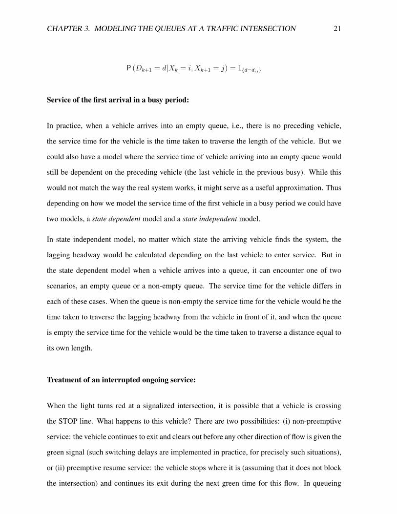
We use a similar model to define the service process in this work except for the fact that we
will assume that the lagging headway for a vehicle is deterministic if its type and the preceding
vehicle’s type are known. i.e.,
CHAPTER 3. MODELING THE QUEUES AT A TRAFFIC INTERSECTION 21
P (Dk+1 = d|Xk = i,Xk+1 = j) = 1{d=dij}
Service of the first arrival in a busy period:
In practice, when a vehicle arrives into an empty queue, i.e., there is no preceding vehicle,
the service time for the vehicle is the time taken to traverse the length of the vehicle. But we
could also have a model where the service time of vehicle arriving into an empty queue would
still be dependent on the preceding vehicle (the last vehicle in the previous busy). While this
would not match the way the real system works, it might serve as a useful approximation. Thus
depending on how we model the service time of the first vehicle in a busy period we could have
two models, a state dependent model and a state independent model.
In state independent model, no matter which state the arriving vehicle finds the system, the
lagging headway would be calculated depending on the last vehicle to enter service. But in
the state dependent model when a vehicle arrives into a queue, it can encounter one of two
scenarios, an empty queue or a non-empty queue. The service time for the vehicle differs in
each of these cases. When the queue is non-empty the service time for the vehicle would be the
time taken to traverse the lagging headway from the vehicle in front of it, and when the queue
is empty the service time for the vehicle would be the time taken to traverse a distance equal to
its own length.
Treatment of an interrupted ongoing service:
When the light turns red at a signalized intersection, it is possible that a vehicle is crossing
the STOP line. What happens to this vehicle? There are two possibilities: (i) non-preemptive
service: the vehicle continues to exit and clears out before any other direction of flow is given the
green signal (such switching delays are implemented in practice, for precisely such situations),
or (ii) preemptive resume service: the vehicle stops where it is (assuming that it does not block
the intersection) and continues its exit during the next green time for this flow. In queueing

CHAPTER 3. MODELING THE QUEUES AT A TRAFFIC INTERSECTION 22
literature there is also the notion of preemptive repeat service, which in this setting would mean
that the vehicle backs up to behind the STOP line, and attempts another exit in the next green
time; this is clearly impractical in the traffic light setting.
We would later see that Webster’s approximation [21] is modeling a preemptive resume service
model. Hence in this work we will also assume the service to be preemptive resume.
3.2 Relation to the PCU terminology:
The PCU is the universally adopted unit of measurement of traffic volume, defined by taking
the passenger car as the standard vehicle. The passenger car has a PCU value equal to 1 and
larger vehicles have PCU values greater than one. There are several different methods used to
define PCU Values. The one we use is a variant of the Headway Ratio Method. The headway
distance means the distance between the front tip of preceding vehicle to the front tip of the
following vehicle.
The Headway Ratio Method is defined as follows
Given ,
Hc =Average Headway for passenger car (averaged over all possible preceding vehicle types)
Hi =Average Headway for vehicle type i (averaged over all possible preceding vehicle types)
Then, PCU value of Vehicle Type i is given by
PCUi = Hi
Hc
Though in Headway Ratio Method, headway means the distance between the front tip of preced-
ing vehicle to the front tip of the following vehicle, a headway defined by the distance between
rear end of preceding vehicle to the rear end of following vehicle (lagging headway) , i.e., tail-
to-tail distances, is considered a more appropriate measurement for estimating PCU values [16].

CHAPTER 3. MODELING THE QUEUES AT A TRAFFIC INTERSECTION 23
So, we use the lagging headway for calculating the PCU values. Thus,
Hi = mean lagging headway for vehicle type i
Hc = mean lagging headway for passenger car
For Xk, k ≥ 0, Xk ∈ V , denoting the indices of the successive vehicles crossing HOL position
at an intersection, let us define the precedence probability as follows,
pij = P [Xk = j|Xk+1 = i] ∀i ∈ V , j ∈ V
We can obtain the pijvalues from the fij values, given the stationary probabilities πi, i ∈ V as
follows
pij = πjfjiπi
If we were to use preceding probabilities pi,j, i, j ∈ V , with vehicle type c denoting passenger
car & tail-to-tail distances dij , then we can define PCU value of Vehicle Type i as
PCUi = γi =Hi
Hc
=∑j∈V pijdji∑j∈V pcjdjc
(3.1)
where expectation over all possible tail-to-tail distances for vehicle type i is taken to compute
the mean lagging headway Hi of vehicle type i.
If the PCU values for each vehicle types, the stationary probability distribution and the mean
service time for a passenger car are given, we can can calculate the mean service time as given
below.
For PCU value [3.1] of vehicle type i, γi, defined by

CHAPTER 3. MODELING THE QUEUES AT A TRAFFIC INTERSECTION 24
γi =∑j∈V pijdji∑j∈V pcjdjc
and mean mean service time for passenger car, τc, given by
τc =
∑j∈V
pcjdjc
vs
the mean service time is given by
τ =
∑i∈Vπi
∑j∈V
pijdji
vs
=
∑i∈Vπiγi
∑j∈V
pcjdjc
vs
=τc∑i∈Vπiγi
3.3 Traffic Intersection Simulation
The scenario of traffic at signalised intersections was simulated in Matlab. The simulations of 3
different models were done. The M/SM/1 model, which is the model that we have discussed till
now, with Poisson arrivals and service process where the successive service times are dependent,
is the primary model studied. We also consider two simplified models derived from the M/SM/1
model. Those would be the M/G/1 model and the M/D/1 model. We assume that we know the
following probabilitiy distribution [3.1.2] for each type of vehicles and the lagging headway for
every pair of vehicle types is also known. It is also assumed that vehicles have zero acceleration
time i.e., the vehicles instantly accelerates to the exit velocity.
1. M/SM/1 model : The inter arrival durations are exponentially distributed. The initial ve-
hicle is sampled from the stationary probability distribution obtained from the following
CHAPTER 3. MODELING THE QUEUES AT A TRAFFIC INTERSECTION 25
probabilities. Every subsequent vehicle is sampled from the following probability distri-
bution of the previous vehicle. The service time for the current vehicle is computed after
looking at the types of current vehicle and the previous vehicle. eg: if current vehicle type
is i and the previous vehicle was of type j, then the service time for vehicle i is taken to
be djivs
(where vsis the exit velocity for vehicles). This is the primary model available.
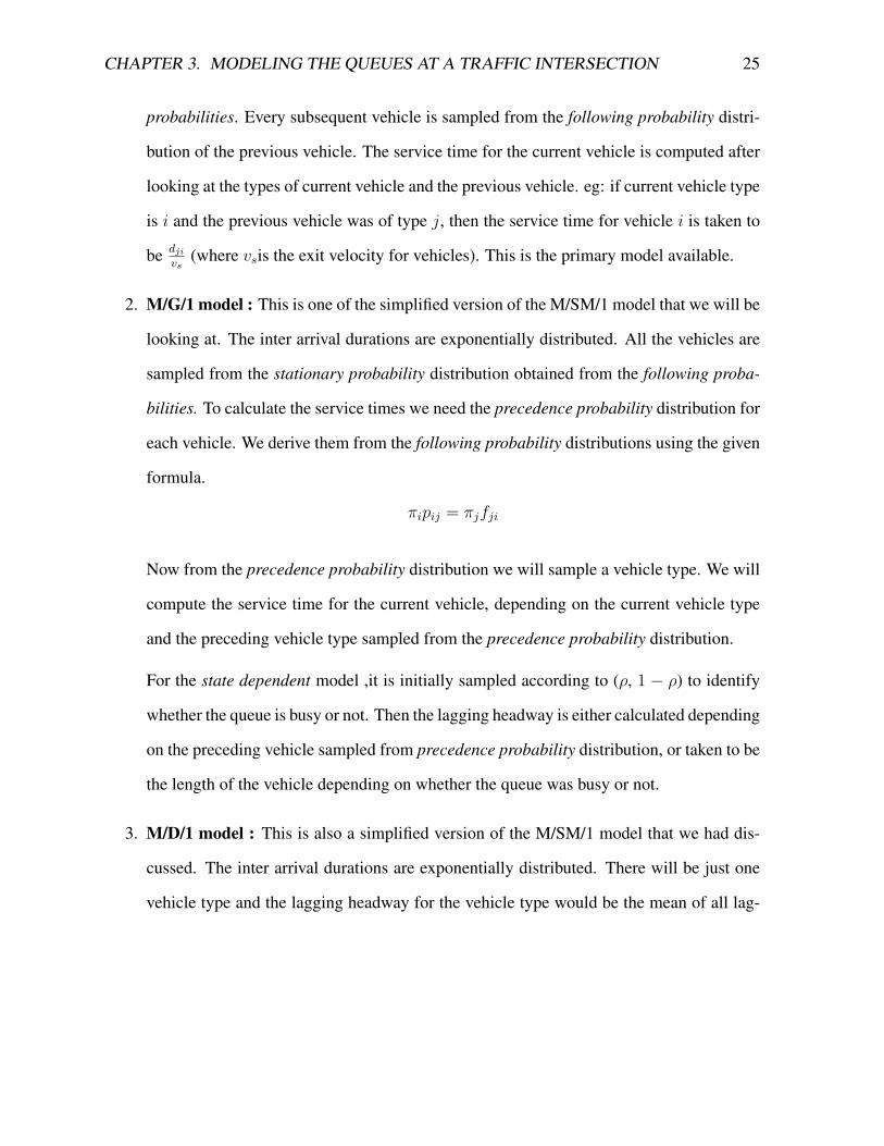
2. M/G/1 model : This is one of the simplified version of the M/SM/1 model that we will be
looking at. The inter arrival durations are exponentially distributed. All the vehicles are
sampled from the stationary probability distribution obtained from the following proba-
bilities. To calculate the service times we need the precedence probability distribution for
each vehicle. We derive them from the following probability distributions using the given
formula.
πipij = πjfji
Now from the precedence probability distribution we will sample a vehicle type. We will
compute the service time for the current vehicle, depending on the current vehicle type
and the preceding vehicle type sampled from the precedence probability distribution.
For the state dependent model ,it is initially sampled according to (ρ, 1 − ρ) to identify
whether the queue is busy or not. Then the lagging headway is either calculated depending
on the preceding vehicle sampled from precedence probability distribution, or taken to be
the length of the vehicle depending on whether the queue was busy or not.
3. M/D/1 model : This is also a simplified version of the M/SM/1 model that we had dis-
cussed. The inter arrival durations are exponentially distributed. There will be just one
vehicle type and the lagging headway for the vehicle type would be the mean of all lag-
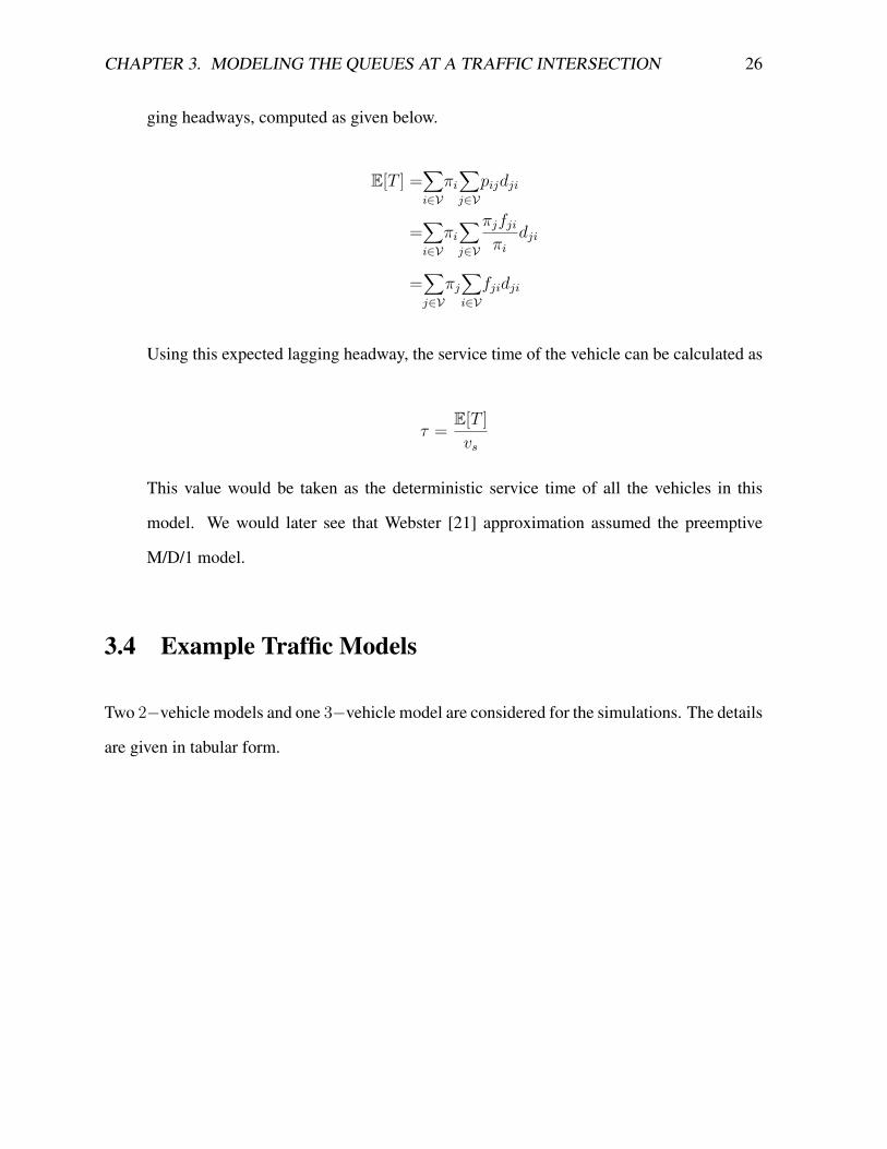
CHAPTER 3. MODELING THE QUEUES AT A TRAFFIC INTERSECTION 26
ging headways, computed as given below.
E[T ] =∑i∈Vπi
∑j∈V
pijdji
=∑i∈Vπi
∑j∈V
πjfjiπi
dji
=∑j∈V
πj∑i∈Vfjidji
Using this expected lagging headway, the service time of the vehicle can be calculated as
τ = E[T ]vs
This value would be taken as the deterministic service time of all the vehicles in this
model. We would later see that Webster [21] approximation assumed the preemptive
M/D/1 model.
3.4 Example Traffic Models
Two 2−vehicle models and one 3−vehicle model are considered for the simulations. The details
are given in tabular form.

CHAPTER 3. MODELING THE QUEUES AT A TRAFFIC INTERSECTION 27
Parameters Traffic Model-1 Traffic Model-2lA 4m 4mlB 14m 30m
{dAA,dAB,dBA,dBB} {5m, 7m, 16m, 18m} {5m, 7m, 33m, 36m}{fAA, fAB, fAB, fBB} {0.5, 0.5, 0.5, 0.5} {0.5, 0.5, 0.5, 0.5}
{πA, πB} {0.5, 0.5} {0.5, 0.5}Cycle length, c 60s 60s
Mean service time, τ (StateIndependent)
2.555s 4.5s
Second moment, b(2)1 8.07 30.358
Variance of service timedistribution
1.546 10.1
Exit Velocity, vs 4.5 m/s 4.5 m/s
Table 3.2: Parameters used for the two traffic models considered for simulations and later, foranalysis
Parameters Traffic Model - 3{lA, lB, lC} {4m, 15m, 30m}
{dAA, dBA, dCA, dAB, dBB,dCB, dAC , dBC , dCC}
{5m, 6m, 8m, 18m, 20m,24m, 34m, 36m, 42m}
{fAA, fAB, fAC , fBA, fBB,fBC , fCA, fCB, fCC}
{0.6, 0.3, 0.1, 0.4, 0.4, 0.2,0.3, 0.3, 0.4}
{πA, πB,πC} {0.4762, 0.3333, 0.1905}Preceding probability Dist.
for A(pAi, i ∈ V){5m, 6m, 8m} w.p. {0.6,
0.28, 0.12}Preceding probability Dist.
for B(PBi, i ∈ V){18m, 20m, 24m} w.p.{0.4286, 0.4, 0.1714}
Preceding probability Dist.for C(PCi, i ∈ V)
{34m, 36m, 42m} w.p.{0.25, 0.35, 0.4}
Mean service time, τ (StateIndependent)
3.67s
Second moment, b(2)1 20.937
Table 3.3: Parameters used for 3 - vehicle case study
CHAPTER 3. MODELING THE QUEUES AT A TRAFFIC INTERSECTION 28
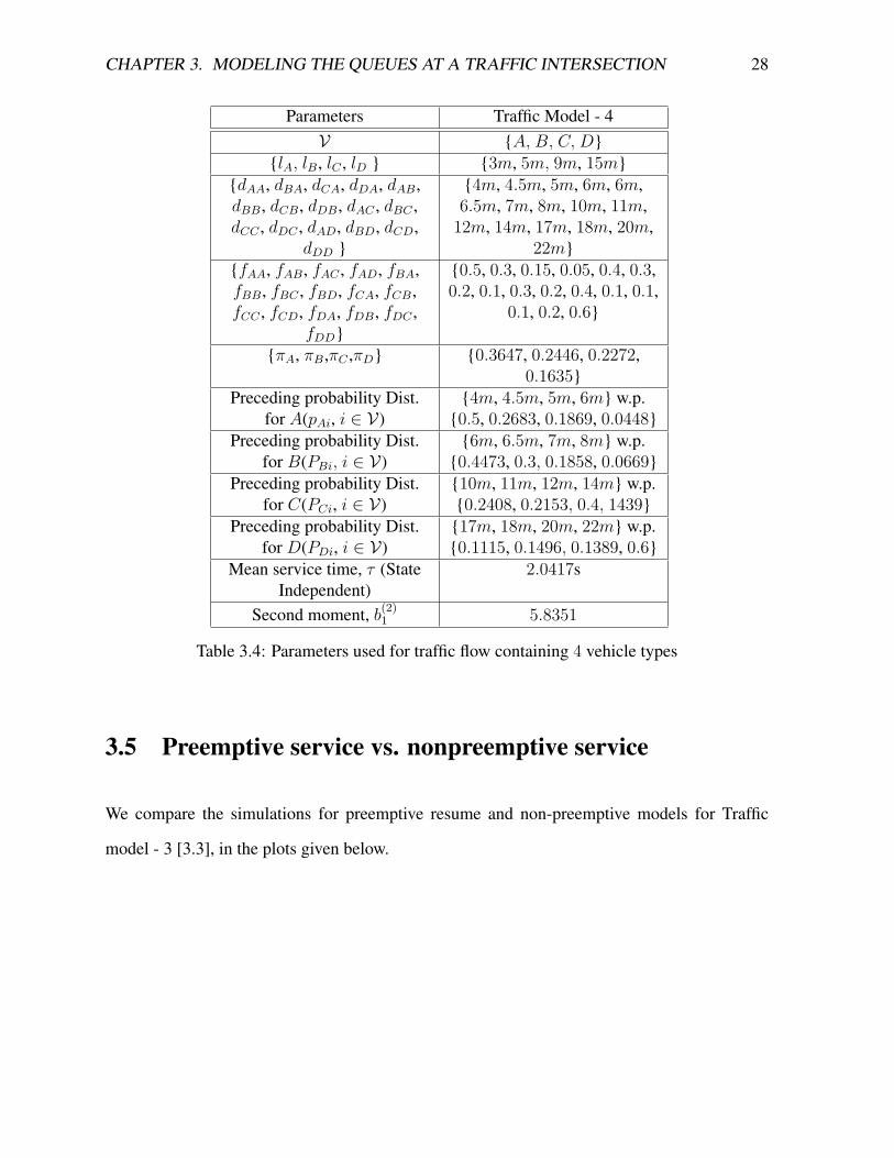
Parameters Traffic Model - 4V {A, B, C, D}
{lA, lB, lC , lD } {3m, 5m, 9m, 15m}{dAA, dBA, dCA, dDA, dAB,dBB, dCB, dDB, dAC , dBC ,dCC , dDC , dAD, dBD, dCD,
dDD }
{4m, 4.5m, 5m, 6m, 6m,6.5m, 7m, 8m, 10m, 11m,
12m, 14m, 17m, 18m, 20m,22m}
{fAA, fAB, fAC , fAD, fBA,fBB, fBC , fBD, fCA, fCB,fCC , fCD, fDA, fDB, fDC ,
fDD}
{0.5, 0.3, 0.15, 0.05, 0.4, 0.3,0.2, 0.1, 0.3, 0.2, 0.4, 0.1, 0.1,
0.1, 0.2, 0.6}
{πA, πB,πC ,πD} {0.3647, 0.2446, 0.2272,0.1635}
Preceding probability Dist.for A(pAi, i ∈ V)
{4m, 4.5m, 5m, 6m} w.p.{0.5, 0.2683, 0.1869, 0.0448}
Preceding probability Dist.for B(PBi, i ∈ V)
{6m, 6.5m, 7m, 8m} w.p.{0.4473, 0.3, 0.1858, 0.0669}
Preceding probability Dist.for C(PCi, i ∈ V)
{10m, 11m, 12m, 14m} w.p.{0.2408, 0.2153, 0.4, 1439}
Preceding probability Dist.for D(PDi, i ∈ V)
{17m, 18m, 20m, 22m} w.p.{0.1115, 0.1496, 0.1389, 0.6}
Mean service time, τ (StateIndependent)
2.0417s
Second moment, b(2)1 5.8351
Table 3.4: Parameters used for traffic flow containing 4 vehicle types
3.5 Preemptive service vs. nonpreemptive service
We compare the simulations for preemptive resume and non-preemptive models for Traffic
model - 3 [3.3], in the plots given below.

CHAPTER 3. MODELING THE QUEUES AT A TRAFFIC INTERSECTION 29
0 0.1 0.2 0.3 0.4 0.5 0.6 0.7 0.8 0.9 10
10
20
30
40
50
60
Degree of Saturation (x)
Nor
mal
ised
Mea
n D
elay
Simulation (SD) : M/D/1 preemptive interruptionSimulation (SD) : M/G/1 preemptive interruptionSimulation (SD) : M/SM/1 preemptive interruptionSimulation (SD) : M/D/1 non − preemptive interruptionSimulation (SD) : M/G/1 non − preemptive interruptionSimulation (SD) : M/SM/1 non − preemptive interruption
(a) Cycle Time = 60s, Green Time = 20s.
0 0.1 0.2 0.3 0.4 0.5 0.6 0.7 0.8 0.9 10
5
10
15
20
25
30
35
40
45
Degree of saturation (x)
Nor
mal
ised
Mea
n D
elay
Simulation (SD) : M/D/1 preemptive interruptionSimulation (SD) : M/G/1 preemptive interruptionSimulation (SD) : M/SM/1 preemptive interruptionSimulation (SD) : M/D/1 non − preemptive interruptionSimulation (SD) : M/G/1 non − preemptive interruptionSimulation (SD) : M/SM/1 non − preemptive interruption
(b) Cycle Time = 60s, Green Time = 50s.
Figure 3.6: Normalised Mean Delay v/s Degree of Saturation (Traffic Model-3) : Comparisonbetween preemptive and non-preemptive simulations of M/D/1, M/G/1 and M/SM/1 models(State Dependent).
In the plots we see that the simulation of non-preemptive model does not match with simulation
of preemptive resume model, which is along expected lines. The non-preemptive simulations
CHAPTER 3. MODELING THE QUEUES AT A TRAFFIC INTERSECTION 30
are expected to differ from the preemptive simulation by quite a margin at higher loads because
, at higher loads it is highly likely to have a vehicle start its service just before the red time.
But since the model is non-preemptive, the work is assumed to have completed during the red
time. This will mean that we would lose out on a large amount of work in non-preemptive
model which we would otherwise consider in the preeemptive model. This would decrease the
mean delays we see at higher loads in the non-preemptive case. Hence there exist a significant
difference in the mean delay seen in the two models. We will see in Chapter 4 Section [4.3.1]
that the well known Webster delay formula matches our simulation with preemptive resume
service. Based on this, we consider preemptive resume to be service model in the rest of this
work.
3.6 Service of the First Arrival in a Busy Period
We will now compare the preemptive interruption traffic Models (M/D/1, M/G/1, M/SM/1) in
state dependent and state independent environments. The plots for the Traffic Model-2 [3.2]
and Traffic Model-3 [3.3] are shown below.
X-Axis degree of saturation = λτg/c
, where τ is the mean service time state independent
model.
Y-Axis Mean Delay

CHAPTER 3. MODELING THE QUEUES AT A TRAFFIC INTERSECTION 31
0 0.1 0.2 0.3 0.4 0.5 0.6 0.7 0.8 0.9 10
20
40
60
80
100
120
140
160
180
200
Degree of Saturation (x)
Mea
n D
elay
Simulation (SD) : M/D/1 preemptive interruptionSimulation (SD) : M/G/1 preemptive interruptionSimulation (SD) : M/SM/1 preemptive interruptionSimulation : M/D/1 preemptive interruptionSimulation : M/G/1 preemptive interruptionSimulation : M/SM/1 preemptive interruption
(a) Cycle Time = 60s, Green Time = 20s.
0 0.1 0.2 0.3 0.4 0.5 0.6 0.7 0.8 0.9 10
20
40
60
80
100
120
140
160
180
Degree of Saturation (x)
Mea
n D
elay
Simulation (SD) : M/D/1 preemptive interruptionSimulation (SD) : M/G/1 preemptive interruptionSimulation (SD) : M/SM/1 preemptive interruptionSimulation : M/D/1 preemptive interruptionSimulation : M/G/1 preemptive interruptionSimulation : M/SM/1 preemptive interruption
(b) Cycle Time = 60s, Green Time = 50s.
Figure 3.7: Normalised Mean Delay V/s Degree of Saturation (Traffic Model-2) : Comparisonbetween preemptive State Dependent simulation and preemptive State Independent simulationmodels.
CHAPTER 3. MODELING THE QUEUES AT A TRAFFIC INTERSECTION 32
0 0.1 0.2 0.3 0.4 0.5 0.6 0.7 0.8 0.9 10
20
40
60
80
100
120
140
160
180
200
Degree of Saturation (x)
Mea
n D
elay
Simulation(SD): M/D/1 preemptive interruptionSimulation(SD): M/G/1 preemptive interruptionSimulation(SD): M/SM/1 preemptive interruptionSimulation: M/D/1 preemptive interruptionSimulation: M/G/1 preemptive interruptionSimulation: M/SM/1 preemptive interruption
(a) Cycle Time = 60s, Green Time = 20s.
0 0.1 0.2 0.3 0.4 0.5 0.6 0.7 0.8 0.9 10
20
40
60
80
100
120
140
160
Degree of Saturation (x)
Mea
n D
elay
Simulation(SD): M/D/1 preemptive interruptionSimulation(SD): M/G/1 preemptive interruptionSimulation(SD): M/SM/1 preemptive interruptionSimulation: M/D/1 preemptive interruptionSimulation: M/G/1 preemptive interruptionSimulation: M/SM/1 preemptive interruption
(b) Cycle Time = 60s, Green Time = 50s.
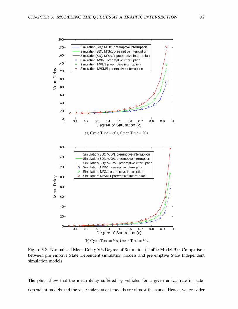
Figure 3.8: Normalised Mean Delay V/s Degree of Saturation (Traffic Model-3) : Comparisonbetween pre-emptive State Dependent simulation models and pre-emptive State Independentsimulation models.
The plots show that the mean delay suffered by vehicles for a given arrival rate in state-
dependent models and the state independent models are almost the same. Hence, we consider

CHAPTER 3. MODELING THE QUEUES AT A TRAFFIC INTERSECTION 33
state independent model in the rest of this work.
3.7 Stability Criterion
Notation
τ mean service requirement for the the set of vehicles V
{X(t), t ≥ 0} the random process representing the work seen in the system at time t.
{Y (t), t ≥ 0} the process constructed from {X(t), t ≥ 0} by deleting the red times.
{Z(t), t ≥ 0} the process constructed from {X(t), t ≥ 0} by deleting the green times.
A state independent service time distribution implies that the service time distribution of all the
vehicles in the queue are identical. Under this assumption, Sengupta [17] gives the following
arguments to provide the stability criterion for the queue with interrupted service.
Gk Rk Gk+1 Rk+1 Gk+2 Rk+2 Gk+3
Gk Gk+1 Gk+2 Gk+3 Rk Rk+1 Rk+2
X(t)
Y(t)Z(t)
work in the system at time 't'
Only Green TimesOnly Red times
M/G/1 + G/G/1
Figure 3.9: This figure show how the {X(t), t ≥ 0} process is split into {Y (t), t ≥ 0} and{Z(t), t ≥ 0} processes. The Gk and Rk values are constants g and r respectively.
From the above figure [3.9] it is obvious that the {Y (t), t ≥ 0} process is identical to, work in

CHAPTER 3. MODELING THE QUEUES AT A TRAFFIC INTERSECTION 34
the system for a queue with a mix of M/G/1 and G/G input streams. The process {X(t), t ≥ 0}
is stable if and only if, the process {Y (t), t ≥ 0} is stable [[17]]. Thus, conditioned on the
green periods, which are the only times during which work is done, we have an M/G/1 queue
and a GI/G/1 queue. The rate of arrival of work in the M/G/1 queue is λτ , and that in the GI/G/1
queue is 1gλτr . Hence the stability condition is given by,
0 ≤ λτ + λτr
g< 1
0 ≤ λτ
g/c< 1
0 ≤ x < 1

Chapter 4
Analysis of Queues at Traffic Intersections
In this chapter we study analytical models for estimating the mean delay experienced by vehi-
cles for the different models that we have discussed.
A model that closely resembles traffic at intersections is queues with interruption [17]. Here
the server randomly takes a break, even in between service. Once it takes a break it stays in
OFF-state for a random amount of time and then returns to service. Again, it will stay on
service for a random time period and then takes a break. This continues. We see that , this
model with ON and OFF durations sampled from a deterministic distribution represent quite
realistically the traffic at intersections. Sengupta [17] analyses the work in the queue , waiting
time distribution etc for a queue with interruptions in detail. Later in this chapter, we use those
results to calculate the mean delay in such queues, and then compare the results against the
mean delay suffered by vehicles calculated using the Webster’s formula [21], and also against
the mean delay suffered by vehicles calculated using simulations of traffic intersections, and see
if the queue with interruptions can give any improvement over the Webster’s results.
We will find that queues with interruption model discussed by Sengupta [17] with appropriate
service distribution approximates the corresponding simulation model quite well, and that the
Webster’s model [21] models the M/D/1 simulation quite well. We will also suggest modified
Webster’s models which will accurately model the M/G/1 and M/SM/1 models quite well.
35

CHAPTER 4. ANALYSIS OF QUEUES AT TRAFFIC INTERSECTIONS 36
Before we look at these models, we will look at a general analysis of mean delay suffered by
arriving vehicles at an intersection.
4.1 Mean Delay Analysis - Preliminaries
Notation
Wk waiting time (time until start of service) for kth vehicle
Vk work in the system seen by kth vehicle, on arrival into the intersection
Rk total red-time encountered by kth vehicle
EW mean waiting time for vehicles at the intersection
EV mean work seen by arrivals into the intersection
ER mean red-time seen by arrivals
V(g)k work seen by the kth vehicle to arrive in the green time
V(r)k work seen by the kth vehicle to arrive in the red time
V (g) mean work seen by an arrival during the green time
V (r) mean work seen by an arrival during the red time
R(g)k red time encountered by the kth vehicle to arrive in the green time
R(r)k red time encountered by the kth vehicle to arrive in the red time
∼Gk residual green time seen by the kth vehicle to arrive in the green time
∼Sk residual red time seen by the kth vehicle to arrive in the red time
ES mean residual red time seen by a vehicle arriving during the red time
CHAPTER 4. ANALYSIS OF QUEUES AT TRAFFIC INTERSECTIONS 37
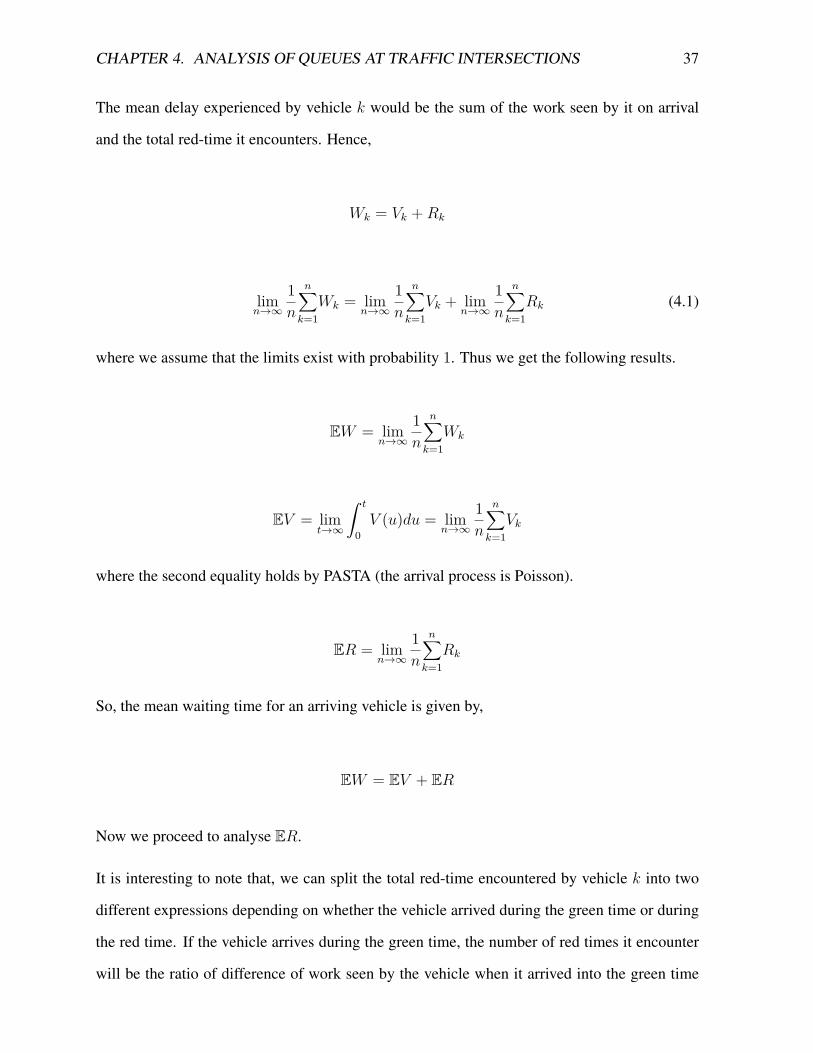
The mean delay experienced by vehicle k would be the sum of the work seen by it on arrival
and the total red-time it encounters. Hence,
Wk = Vk +Rk
limn→∞
1n
n∑k=1
Wk = limn→∞
1n
n∑k=1
Vk + limn→∞
1n
n∑k=1
Rk (4.1)
where we assume that the limits exist with probability 1. Thus we get the following results.
EW = limn→∞
1n
n∑k=1
Wk
EV = limt→∞
ˆ t
0V (u)du = lim
n→∞
1n
n∑k=1
Vk
where the second equality holds by PASTA (the arrival process is Poisson).
ER = limn→∞
1n
n∑k=1
Rk
So, the mean waiting time for an arriving vehicle is given by,
EW = EV + ER
Now we proceed to analyse ER.
It is interesting to note that, we can split the total red-time encountered by vehicle k into two
different expressions depending on whether the vehicle arrived during the green time or during
the red time. If the vehicle arrives during the green time, the number of red times it encounter
will be the ratio of difference of work seen by the vehicle when it arrived into the green time

CHAPTER 4. ANALYSIS OF QUEUES AT TRAFFIC INTERSECTIONS 38
and the residual time of the current green time during which it arrived, to the duration of a
green time , rounded to the nearest higher integer value (ceil function), and if the vehicle arrives
during the red time, the number of red times it encounter will be, the ratio of work seen by the
vehicle when it arrived into the red time to the duration of a green time, rounded to the nearest
lower integer value (floor function) plus the residual time of the current red time during which
it arrived. This can be expressed as follows.
If the vehicle k arrives during green time, the total red-time it encounters will be,
R(g)k =
V(g)k −
∼Gk
g
rand if the vehicle k arrives during red time, the total red-time it counters will be,
R(r)k =
∼Sk +
V (r)k −
∼Sk
g
rThis allows us to define the mean red-time encountered by a vehicle to be,
ER = g
r + gE[R(g)
k ] + r
r + gE[R(r)
k ] (4.2)
We will now approximate is, R(g)k and R(r)
k as follows
R(g)k = V
(g)k
gr
R(r)k =
∼Sk + V
(r)k
gr
Also, it is clear that

CHAPTER 4. ANALYSIS OF QUEUES AT TRAFFIC INTERSECTIONS 39
EV = g
g + rV (g) + r
g + rV (r)
Since for a deterministic distribution of red time, the mean residual time is given by
ES = r
2
Using the approximations forR(g)k andR(r)
k as given above, the mean waiting time for an arriving
vehicle will become
EW =EV + r
gEV + r
cES (4.3)
= c
gEV + r2
2c
We will later see in Section [5.1] that the first term in the above expression, which is the mean
work expanded by a factor of cg, gives the mean delay suffered by an arriving vehicle assuming
the server is active at the instant just after arrival. The second term is the mean time the vehicle
has to wait till the server gets active for the first time after arrival.
4.2 The Analysis in Sengupta [17]
This model provides an accurate depiction of a traffic intersection from queueing point of view.
This model considers a queue in a random environment defined by an alternating renewal pro-
cess. The states of the alternating renewal process are 1 (ON) and 2 (OFF). The distribution of
time spent in state i (i = 1,2) is Fi(t). Arrivals in state i occur according to a poisson process
with mean rate λi. The service time distribution is given by Bi(t). The service times of succes-
sive customers are assumed to be independent. This model splits the process {X(t), t ≥ 0},
the amount of work in the system at time t, into two stationary processes {Y (t), t ≥ 0}, {Z(t),
CHAPTER 4. ANALYSIS OF QUEUES AT TRAFFIC INTERSECTIONS 40
t ≥ 0}. Y (t) is constructed from process X(t) by deleting all times when environment is in
state 2, and Z(t) by deleting all times when environment is in state 1. Then [17] proceeds to
compute the mean work in the process Y (t) and Z(t), and proportionally combining them to
obtain the mean work in the system , X(t). In the following expressions∼B1(s) denotes the LST
of B1(t), and b(k)i (t) denotes kth moment of Bi(t).
G(t) distribution of work brought in at renewal epochs of Y (t). (i.e work accumulated
during the previous OFF period)
∼ρ(s) LST of busy period of a special M/G/1 queue with arrival λ1, and service time
distribution B1(t) whose amount of work at time 0 is given by the distribution
G(t).
A special GI/GI/1 queue is defined, with inter-arrival duration F1(t) and LST of service time
distribution is ∼ρ(s).
∼V (s) LST of work in the special GI/G/1 queue.
∼W (s) LST of customer arrival stationary distribution of the special GI/G/1 queue.
∼U(s) LST of steady-state distribution of, Z(t) observed at instants just after the renewal
epochs.
We saw in the mean delay equation in the general approach [4.3] that the mean delay suffered
by vehicles have two components, the work seen by the arrivals which is scaled by a factor of cg,
and the mean residual red time seen by arrivals that happen during the red times. This motivates
us to find an expression for mean work in the system to calculate the mean delay suffered by an
arriving vehicle into the intersection (queue).
4.2.1 Mean Work in the System
Then according to Sengupta [17] Y (t) can be shown as the decomposition of work in a special
GI/G/1 queue and an M/G/1 queue.

CHAPTER 4. ANALYSIS OF QUEUES AT TRAFFIC INTERSECTIONS 41
The steady state LST of the process Y (t),∼R1(s) is given by
∼R1(s) = 1− λ1b
(1)1
1− λ1[(1−∼B1(s))/s]
.∼V (s− λ1(1−
∼B1(s))) (4.4)
Then the expected value of work in the system for the process {Y (t), t ≥ 0} is
r(1)1 = λ1b
(2)1
2(1− λ1b(1)1 )
+ (1− λ1b(1)1 )v(1) (4.5)
Similarly,
∼U(s) = 1− λ1b
(1)1
1− λ1[(1−∼B1(s))/s]
.∼W (s− λ1(1−
∼B1(s))) (4.6)
and its expected value is given by
u(1) = λ1b(2)1
2(1− λ1b(1)1 )
+ (1− λ1b(1)1 )w(1) (4.7)
The relationship between v(1) and w(1) is given by
v(1) = ρ(2)
2f (1)1
+ ρ(1)
f(1)1w(1) (4.8)
(The 2 in [4.8] is missing in [17]).
The LST of steady-state distribution of Z(t),∼R2(s) is ,
∼R2(s) =
∼U(s)(1−
∼F2(λ2(1−
∼B2(s))))
f(1)2 λ2(1−
∼B2(s))
(4.9)
and its mean is given by,

CHAPTER 4. ANALYSIS OF QUEUES AT TRAFFIC INTERSECTIONS 42
r(1)2 = u(1) + λ2b
(1)2 f
(2)2
2f (1)2
(4.10)
The expected work in the system for process {X(t), t ≥ 0} is
r(1) = c1r(1)1 + c2r
(1)2 (4.11)
r(1) = λ1b(2)1
2(1− λ1b(1)1 )
+ (1− λ1b(1)1 )(c1v
(1) + c2w(1)) + c2λ2b
(1)2 f
(2)2
2f (1)2
where,
c1 = f(1)1
f(1)1 + f
(1)2
; c2 = 1− c1 (4.12)
Thus the equation [4.11] gives the mean work seen by an arrival into the queue (by PASTA as
arrivals are Poisson distributed).
4.2.2 Mean Waiting Time
Sengupta [17] provides an analysis of mean waiting time in interrupted queues. We would look
at this method of analysis and will conclude that the mean delay obtained by Sengupta reduces
to the form of the mean delay expression that we had arrived at earlier [4.3].
To analyze the waiting-time distribution, [17] distinguishes between two types of customers,
those who arrive during ON-period and those who arrive during OFF-period. For a customer
who arrives during ON-period and sees x units of work, the waiting period must be x plus the
length of the OFF-periods that occur during the depletion of the x units of work. Lets us define
the following parameters.
Πi(t, x)dt is the joint probability density of

CHAPTER 4. ANALYSIS OF QUEUES AT TRAFFIC INTERSECTIONS 43
1. environment being in state i
2. time spent in state i element of (t, t+ dt)
3. amount of work in the system is less than or equal to x
Wi(t, x, y) probability that the waiting time is less than or equal to y given that a customer
arrives when the environment is in state i(= 1, 2), elapsed time in state i at the
instant of arrival is t and the work in the system seen by the arrival is x
w(1)i (t, x) the expectation of the distribution of Wi(t, x, y) for i = 1, 2
N(t, x) no:of renewals in [0, x] for a delayed renewal process whose first renewal time has
a distribution F1(t+z)/(1−F1(t)) and has distribution F1(t) from second renewal
time onwards
Wq waiting time of a randomly chosen customer
m(t, x) E[N(t, x)]
The mean waiting times for customers arriving during ON-periods and OFF-periods are given
by.
w(1)1 (t, x) = x+ f
(1)2 m(t, x)
w(1)2 (t, x) =
ˆ ∞0
zdF2(t+ z)1− F2(t) + w
(1)1 (0, x)
The waiting time distribution of a randomly chosen customer is given by,
P (Wq ≤ y) = 1λ
2∑i=1
ˆ ∞0
ˆ ∞0
λiΠi(t, dx)Wi(t, x, y)dt
Taking expectation we get,
CHAPTER 4. ANALYSIS OF QUEUES AT TRAFFIC INTERSECTIONS 44
EWq = 1λ
2∑i=1
ˆ ∞0
ˆ ∞0
λiΠi(t, dx)w(1)i (t, x)dt (4.13)
= λ−1(K + λ1f(1)2 I1 + λ2c2f
(1)2 I2)
where,
K = λ1c1r(1)1 + λ2c2(r(1)
2 + f(2)2
2f (1)2
)
I1 =∞̂
0
∞̂
0
Π1(t, dx)m(t, x)dt
I2 =∞̂
0
dR2(x)m(0, x)
and the overall arrival rate into the system, λ is defined by,
λ = λ1c1 + λ2c2 [4.12]
4.2.3 Approximations for Mean Delay
To get approximate values of I1,∼Π1(t, s)is approximated by
∼Πi(t, s) ≈ c1
(1− F1(t))f
(1)1
∼R1(s).
Here the approximation is that, we assume the work seen by a customer is independent of how
deep into the green time he arrives. This needn’t always be true. Its quite intuitive to see that
ideally the work seen by customer tends to be lesser when he arrives late into the green time.
CHAPTER 4. ANALYSIS OF QUEUES AT TRAFFIC INTERSECTIONS 45
Also, by using the results of the equilibrium renewal process, we have
ˆ ∞0
(1− F1(t))f
(1)1
m(t, x)dt = x
f(1)1.
Thus we have,
I1 ≈c1r
(1)1
f(1)1
(4.14)
.
For calculating I2, [17]gives the approximation,
m(0, x) ≈ x
f(1)1
+ f(2)1
2[f (1)1 ]2
− 1
.
This gives ,
I2 ≈r
(1)2
f(1)2
+ f(2)1
2[f (1)1 ]2− 1 (4.15)
.
Sengupta [17] also gives approximations for the case where F1(t) is deterministic. For this case,
x+ t
f(1)1− 1 6 m(t, x) 6 x+ t
f(1)1
for 0 6 t 6 f(1)1 . Using the above expression,
1f
(1)1
c1r(1)1 + c1f
(2)1
2f (1)1
− c1 6 I1 61f
(1)1
c1r(1)1 + c1f
(2)1
2f (1)1
(4.16)
and

CHAPTER 4. ANALYSIS OF QUEUES AT TRAFFIC INTERSECTIONS 46
r(1)2
f(1)1− 1
6 I2 6r
(1)2
f(1)1
We see that for calculating I1& I2, the computation of r(1)1 & r
(1)2 are required. This in turn
requires the computation of w(1), mean waiting time of the special GI/G/1 queue. We use an
approximation for this calculation. Lets us define the following parameters,
TA inter arrival time of GI/G/1 queue
TH service time of GI/G/1 queue
TW waiting time of GI/G/1 queue
h = E[TH] ; A = E[TH]E[TA] ; C2
A = V ar(TA)E[TA]2 ; C2
H = V ar(TH)E[TH]2
The mean waiting time in a GI/G/1 queue has been approximated [6] to
E[TW ] ≈ Ah
2(1− A)(C2A + C2
H)
e−2(1−A)
3A(1−C2
A)2
C2A
+C2H
, if C2A ≤ 1 (4.17)
≈ Ah
2(1− A)(C2A + C2
H)
e−(1−A)(C2A−1)
C2A
+4C2H
, if C2A ≥ 1 (4.18)
4.2.4 Numerical Comparison Between Various Approximations
We compare the M/G/1 preemptive simulation with 4 approximations from the Queues with
Interruption Model. The details for the traffic models used are given in [3.2].
The plots for each case are shown below.
lower bound uses the lower bound values for I1 and I2 from [4.16]
upper bound uses the upper bound values for I1and I2 from [4.16]

CHAPTER 4. ANALYSIS OF QUEUES AT TRAFFIC INTERSECTIONS 47
general approx uses the approximations given for I1and I2 in [4.14] and [4.15]
modified approx uses the approximation [4.14] for I1 and uses the upper bound of [4.16] for
I2
X-Axis degree of saturation = λτg/c
Y-Axis Mean Delay per mean Service Time = Mean Delayτ

CHAPTER 4. ANALYSIS OF QUEUES AT TRAFFIC INTERSECTIONS 48
0 0.1 0.2 0.3 0.4 0.5 0.6 0.7 0.8 0.9 1−10
0
10
20
30
40
50
Degree of Saturation (x)
Nor
mal
ised
Mea
n D
elay
Simulation: M/G/1 preemptive interruptionApprox: M/G/1 preemptive interruption(lower bound)Approx: M/G/1 preemptive interruption(upper bound)Approx: M/G/1 preemptive interruption(general approx)Approx: M/G/1 preemptive interruption(modified approx)
(a) Cycle Time = 60s, Green Time = 20s.
0 0.1 0.2 0.3 0.4 0.5 0.6 0.7 0.8 0.9 1−5
0
5
10
15
20
25
30
35
40
45
Degree of Saturation (x)
Nor
mal
ised
Mea
n D
elay
Simulation: M/G/1 preemptive interruptionApprox: M/G/1 preemptive interruption(lower bound)Approx: M/G/1 preemptive interruption(upper bound)Approx: M/G/1 preemptive interruption(general approx)Approx: M/G/1 preemptive interruption(modified approx)
(b) Cycle Time = 60s, Green Time = 50s
Figure 4.1: Normalised Mean Delay V/s Degree of Saturation (Traffic Model-1) : Comparisonbetween M/G/1 preemptive simulation, M/D/1 preemptive simulation and Queues with Inter-ruption model using different approximations.

CHAPTER 4. ANALYSIS OF QUEUES AT TRAFFIC INTERSECTIONS 49
0 0.1 0.2 0.3 0.4 0.5 0.6 0.7 0.8 0.9 1−5
0
5
10
15
20
25
30
35
40
45
Degree of Saturation (x)
Nor
mal
ised
Mea
n D
elay
Simulation: M/G/1 preemptive interruptionApprox: M/G/1 preemptive interruption(lower bound)Approx: M/G/1 preemptive interruption(upper bound)Approx: M/G/1 preemptive interruption(general approx)Approx: M/G/1 preemptive interruption(modified approx)
(a) Cycle Time = 60s, Green Time = 20s.
0 0.1 0.2 0.3 0.4 0.5 0.6 0.7 0.8 0.9 1−5
0
5
10
15
20
25
30
35
Degree of Saturation (X)
Nor
mal
ised
Mea
n D
elay
Simulation: M/G/1 preemptive interruptionApprox: M/G/1 preemptive interruption(lower bound)Approx: M/G/1 preemptive interruption(upper bound)Approx: M/G/1 preemptive interruption(general approx)Approx: M/G/1 preemptive interruption(modified approx)
(b) Cycle Time = 60s, Green Time = 50s.
Figure 4.2: Normalised Mean Delay V/s Degree of Saturation (Traffic Model-2) : Compar-ison between M/G/1 preemptive simulation , M/D/1 preemptive simulation and Queues withInterruption model using different approximations.
From the plots we see that the modified approximation, that uses the approximation [4.14] for

CHAPTER 4. ANALYSIS OF QUEUES AT TRAFFIC INTERSECTIONS 50
I1 and uses the upper bound of [4.16] for I2 matches really well with the M/G/1 model. Hence
we will be using this approximation from now on. Also here on, the modified approximation
will be refered to as M/G/1 preemptive interruption approximation.
Simplifying the Mean Waiting Time expression from Sengupta
Applying the M/G/1 preemptive interruption approximation [4.2.4] to the expression for mean
waiting time [4.13], we get
I1 ≈c1r
(1)1
f(1)1
= c1r(1)1g
I2 ≈r
(1)2
f(1)1
= r(1)2g
K ≈λ1c1r(1)1 + λ2c2(r(1)
2 + f(2)2
2f (1)2
)
≈λc1r(1)1 + λc2(r(1)
2 + r2
2r )
Thus the mean waiting time becomes,
EWq ≈λ−1(K + λ1f(1)2 I1 + λ2c2f
(1)2 I2)
≈λ−1(K + λrI1 + λc2rI2)
≈c1r(1)1 + c2r
(1)2 + r
g(c1r
(1)1 + c2r
(2)2 ) + c2r
2
= c
gr(1) + r2
2c (4.19)

CHAPTER 4. ANALYSIS OF QUEUES AT TRAFFIC INTERSECTIONS 51
We see that the mean waiting time expression for preemptive M/G/1 Interrupted queue model
[[17]] matches the form of mean delay formula that we had computed earlier [4.3].
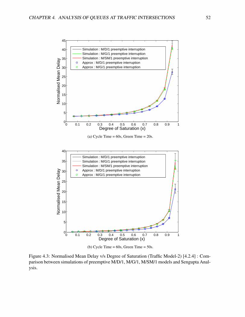
4.2.5 Comparison between the Approximation [4.19] and Simulation
In the plots given below we will compare the Sengupta analysis with the simulations of the
model that we have for traffic at signalized intersections.
CHAPTER 4. ANALYSIS OF QUEUES AT TRAFFIC INTERSECTIONS 52
0 0.1 0.2 0.3 0.4 0.5 0.6 0.7 0.8 0.9 10
5
10
15
20
25
30
35
40
45
Degree of Saturation (x)
Nor
mal
ised
Mea
n D
elay
Simulation : M/D/1 preemptive interruptionSimulation : M/G/1 preemptive interruptionSimulation : M/SM/1 preemptive interruptionApprox : M/D/1 preemptive interruptionApprox : M/G/1 preemptive interruption
(a) Cycle Time = 60s, Green Time = 20s.
0 0.1 0.2 0.3 0.4 0.5 0.6 0.7 0.8 0.9 10
5
10
15
20
25
30
35
40
Degree of Saturation (x)
Nor
mal
ised
Mea
n D
elay
Simulation : M/D/1 preemptive interruptionSimulation : M/G/1 preemptive interruptionSimulation : M/SM/1 preemptive interruptionApprox : M/D/1 preemptive interruptionApprox : M/G/1 preemptive interruption
(b) Cycle Time = 60s, Green Time = 50s.
Figure 4.3: Normalised Mean Delay v/s Degree of Saturation (Traffic Model-2) [4.2.4] : Com-parison between simulations of preemptive M/D/1, M/G/1, M/SM/1 models and Sengupta Anal-ysis.

CHAPTER 4. ANALYSIS OF QUEUES AT TRAFFIC INTERSECTIONS 53
0 0.1 0.2 0.3 0.4 0.5 0.6 0.7 0.8 0.9 10
10
20
30
40
50
60
Degree of Saturation (x)
Nor
mal
ised
Mea
n D
elay
Simulation : M/D/1 preemptive interruptionSimulation : M/G/1 preemptive interruptionSimulation : M/SM/1 preemptive interruptionApprox : M/D/1 preemptive interruptionApprox : M/G/1 preemptive interruption
(a) Cycle Time = 60s, Green Time = 20s.
0 0.1 0.2 0.3 0.4 0.5 0.6 0.7 0.8 0.9 10
5
10
15
20
25
30
35
40
45
50
Degree of Saturation (x)
Nor
mal
ised
Mea
n D
elay
Simulation : M/D/1 preemptive interruptionSimulation : M/G/1 preemptive interruptionSimulation : M/SM/1 preemptive interruptionApprox : M/D/1 preemptive interruptionApprox : M/G/1 preemptive interruption
(b) Cycle Time = 60s, Green Time = 50s.
Figure 4.4: Normalised Mean Delay v/s Degree of Saturation (Traffic Model-3) [4.2.4] : Com-parison between simulations of preemptive M/D/1, M/G/1, M/SM/1 models ans Sengupta Anal-ysis.

CHAPTER 4. ANALYSIS OF QUEUES AT TRAFFIC INTERSECTIONS 54
0 0.1 0.2 0.3 0.4 0.5 0.6 0.7 0.8 0.9 10
5
10
15
20
25
30
35
40
45
50
Degree of Saturation
Nor
mal
ised
Mea
n D
elay
Simulation : M/D/1 preemptive interruptionSimulation : M/G/1 preemptive interruptionSimulation : M/SM/1 preemptive interruptionApprox : M/D/1 preemptive interruptionApprox : M/G/1 preemptive interruption
(a) Cycle Time = 60s, Green Time = 20s.
0 0.1 0.2 0.3 0.4 0.5 0.6 0.7 0.8 0.9 10
2
4
6
8
10
12
14
16
Degree of Saturation (x)
Nor
mal
ised
Mea
n D
elay
Simulation : M/D/1 preemptive interruptionSimulation : M/G/1 preemptive interruptionSimulation : M/SM/1 preemptive interruptionAnalysis : M/D/1 preemptive interruptionAnalysis : M/G/1 preemptive interruption
(b) Cycle Time = 60s, Green Time = 50s.
Figure 4.5: Normalised Mean Delay v/s Degree of Saturation (Traffic Model-4) [4.2.4] : Com-parison between simulations of preemptive M/D/1, M/G/1, M/SM/1 models ans Sengupta Anal-ysis.
From the plots we see that Sungupta analysis works really well for both M/D/1 and M/G/1
service models. Sengupta analysis assumes successive service times to be independent. It would

CHAPTER 4. ANALYSIS OF QUEUES AT TRAFFIC INTERSECTIONS 55
be very difficult to extend the whole of Sengupta analysis for semi Markov service models.
Also, no closed form expressions are available for analysing the delay in M/SM/1 queues. So
we will look at other analytical models to see if we could find approximations for the interrupted
queues with semi Markov service.
4.3 Webster’s Approximation
Webster [21] gives an expression to calculate the mean delay suffered by vehicles while waiting
at a traffic intersection. The expression is
d = r2
2c(1− gcx) + x2
2λ(1− x) − 0.65( cλ2 ) 1
3x2+5 gc (4.20)
We will analyse each term of Webster’s formula seperately. To explain the first term assume the
following. One, traffic arriving is fluid. Two, the traffic arriving during red time gets cleared
exactly at the end of green time.
r g
rλ
slope = λ slope = s-λ
Figure 4.6: Fluid arrival of traffic and traffic arriving during red times getting serviced exactlyin the green times.
From the figure [4.6] the total queue occupancy during the whole period is the area under the
graph. This is,

CHAPTER 4. ANALYSIS OF QUEUES AT TRAFFIC INTERSECTIONS 56
=12(r + g)rλ
=12(r + rλ
s− λ)rλ
=12r2sλ
s− λ
The total queue occupancy is over a full cycle time (c = g + r). So, average queue occupancy
during the cycle =12r2sλs−λc
= 12r2sλ
(s−λ)c . Hence we get from Little’s Theorem, the mean delay =
1λ
12r2sλ
(s−λ)c . Now, substituting r = c − g, we get mean delay = 12c(1− g
c)2
(1−λs
) . Using the fact that
x = λgcs, we get, λ
s= g
cx. Substituting this we get, mean delay = 1
2c(1− g
c)2
(1− gcx) . This gives the first
term of Webster’s expression. Thuswe see that the first term of Webster’s expression gives the
mean delay suffered by a fluid traffic, when the traffic arriving during red time is completely
cleared during the green time. Newell[12] discusses that this term gives a good approximation
for the mean delay, when the arrival rate is less and not close to the saturation flow value. We
would find later in this section by term-by-term comparison with the simulations that this term
together with a correction term, also approximates the mean residual red time seen by arrivals
into the red time [4.3].
When the arrival rate increases, it is not reasonable to assume that the work arriving in a cycle
empties during that cycle itself. There will be work that overflows from one cycle to the next
cycle. The mean overflow queue length is the mean length of the queue at the end of a green
period. Newell [12] gives an approximation for the contribution of the overflow queue to the
mean delay seen at a signalised intersection. Clearly, the mean delay only depends on the mean
queue length and not on the order in which the vehicles are served. So at higher arrival rates,
when the mean overflow queue length is non-zero, let us consider that the server serves in a last
come first served manner. The new arrivals which are served first will see mean delay same as
the first term of Webster’s expression. The mean overflow queue length present at the beginning
of the cycle would approximately encounter a delay of, r+g = c, per cycle. Thus, Newell gives
the approximation for mean delay as,

CHAPTER 4. ANALYSIS OF QUEUES AT TRAFFIC INTERSECTIONS 57
d ≈ r2
2c(1− gcx) + cE[Q0]
cλ
where E[Q0] is the mean overflow queue length. So this must be what Webster was trying to
approximate using his second and third terms.
The mean delay in a M/D/1 queue is given by, ρ2
2λ(1−ρ) . For a service rate reduced by a factor ofgc , we get ρ = λ
gcs
= x. Using this, we get the mean delay of an M/D/1 queue to be equal to
x2
2λ(1−x) . This gives the second term in Webster’s equation. Thus the second term in Webster’s
equation is actually the mean delay suffered in an uninterrupted M/D/1 queue for an arrival
rate given by λ and service rate, sgc. We would find later that this term along with part of
the correction term provides an approximation for the mean delay experienced by an arrival
excluding the residual red times.
The third term in Webster’s expression is an empirical correction term for higher loads used by
Webster [21].
4.3.1 What is Webster’s Formula Approximating?
We compare the Webster approximation with the simulations of the three models that we are
considering (M/D/1, M/G/1 and M/SM/1). The details for Traffic model 2 and 3 are given in
Table [3.2] and [3.3].

CHAPTER 4. ANALYSIS OF QUEUES AT TRAFFIC INTERSECTIONS 58
0 0.1 0.2 0.3 0.4 0.5 0.6 0.7 0.8 0.9 10
5
10
15
20
25
30
35
40
45
50
Degree of Saturation (x)
Nor
mal
ised
Mea
n D
elay
Simulation: M/D/1 preemptive interruptionSimulation: M/G/1 non−preemptive interruptionSimulation: M/G/1 preemptive interruptionApprox: Webster M/D/1
(a) Cycle Time = 60s, Green Time = 20s.
0 0.1 0.2 0.3 0.4 0.5 0.6 0.7 0.8 0.9 10
5
10
15
20
25
30
35
Degree of Saturation (x)
Nor
mal
ised
Mea
n D
elay
Simulation: M/D/1 preemptive interruptionSimulation: M/G/1 non−preemptive interruptionSimulation: M/G/1 preemptive interruptionApprox: Webster M/D/1
(b) Cycle Time = 60s, Green Time = 50s.
Figure 4.7: Normalised Mean Delay v/s Degree of Saturation (Traffic Model-1) : Comparisonbetween M/G/1 simulation (preemptive and non preemptive), M/D/1 preemptive simulation andWebster’s approximation.
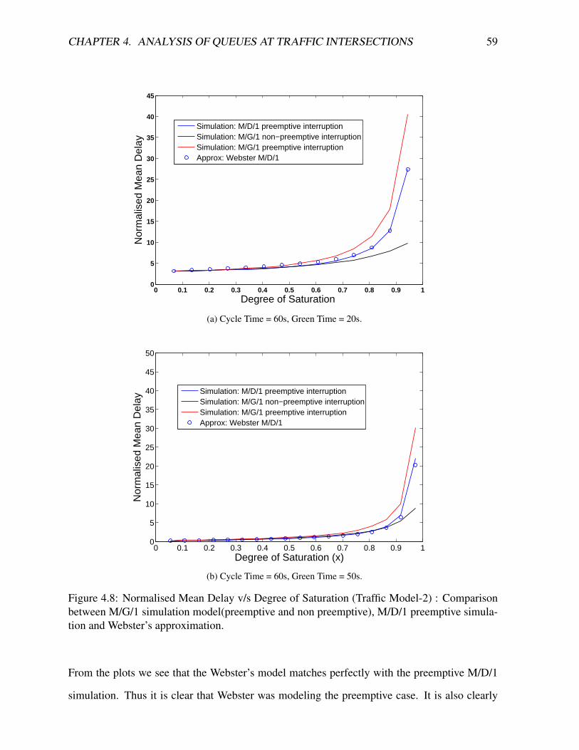
CHAPTER 4. ANALYSIS OF QUEUES AT TRAFFIC INTERSECTIONS 59
0 0.1 0.2 0.3 0.4 0.5 0.6 0.7 0.8 0.9 10
5
10
15
20
25
30
35
40
45
Degree of Saturation
Nor
mal
ised
Mea
n D
elay
Simulation: M/D/1 preemptive interruptionSimulation: M/G/1 non−preemptive interruptionSimulation: M/G/1 preemptive interruptionApprox: Webster M/D/1
(a) Cycle Time = 60s, Green Time = 20s.
0 0.1 0.2 0.3 0.4 0.5 0.6 0.7 0.8 0.9 10
5
10
15
20
25
30
35
40
45
50
Degree of Saturation (x)
Nor
mal
ised
Mea
n D
elay
Simulation: M/D/1 preemptive interruptionSimulation: M/G/1 non−preemptive interruptionSimulation: M/G/1 preemptive interruptionApprox: Webster M/D/1
(b) Cycle Time = 60s, Green Time = 50s.
Figure 4.8: Normalised Mean Delay v/s Degree of Saturation (Traffic Model-2) : Comparisonbetween M/G/1 simulation model(preemptive and non preemptive), M/D/1 preemptive simula-tion and Webster’s approximation.
From the plots we see that the Webster’s model matches perfectly with the preemptive M/D/1
simulation. Thus it is clear that Webster was modeling the preemptive case. It is also clearly
CHAPTER 4. ANALYSIS OF QUEUES AT TRAFFIC INTERSECTIONS 60
evident that the M/G/1 simulation and M/D/1 simulations gives significantly different delays
at higher values of degrees of saturation [3] i.e. when rate of arrival is high for given service
distribution. But an M/D/1 model is not realistic for a traffic intersection. The different vehicles
realistically will have different service times, depending on which type of vehicle precedes it.
But Webster’s approximation does not match well with the preemptive M/G/1 simulation. If we
could understand each term of Webster’s approximation better and identify what exactly each
term is approximating, then we might be able to find an extension of Webster’s analysis for
M/G/1 and M/SM/1.
Chapter 5
Understanding and Extending Webster’s
Formula
In the previous chapter we saw that the Webster’s approximation matches the preemptive M/D/1
simulation, i.e., the M/D/1 interrupted queue. We also discussed about Webster’s intuition
behind each term in his formula, where the first term is the mean delay assuming that the mean
overflow queue length is zero (which is a good approximation for low arrival rates), and the
second term represents the contribution of mean overflow queuelength to the mean delay (which
is significant at higher arrival rates). In this chapter we will compare the terms from Webster’s
formula with the general mean delay formula [4.3] and Sengupta approximation for mean delay
[4.19], i.e., we will identify which component in the mean delay suffered by vehicles at an
intersection [4.3], each of the terms are trying to approximate.
5.1 Understanding Webster’s Approximation
At an intersection a vehicle can arrive either during a green period or a red period. If it arrives
during a red period, it has to wait for the remaining red time to end before the server becomes
active. But this is zero for a vehicle arriving during the green time. Here we compare the delay
61
CHAPTER 5. UNDERSTANDING AND EXTENDING WEBSTER’S FORMULA 62
due to mean residual red time and the mean delay experienced excluding the mean residual
red time, for an arriving vehicle, from the simulations with the mean residual red time and
the expanded mean work [4.19] for the approximation by Sengupta (M/D/1) [17] [4.19] and the
fluid approximation term and the M/D/1 mean delay term from Webster’s approximation [4.20].

CHAPTER 5. UNDERSTANDING AND EXTENDING WEBSTER’S FORMULA 63
0 0.1 0.2 0.3 0.4 0.5 0.6 0.7 0.8 0.9 10
5
10
15
20
25
Degree of Saturation
Nor
mal
ised
Mea
n D
elay
Simulation : M/D/1 preemptive interruption (mean delay excluding residual red times)Simulation : M/D/1 preemptive interruption (mean delay due to residual red times)Analysis : M/D/1 preemptive interruption (mean delay excluding residual red times)Analysis : M/D/1 preemptive interruption (mean delay due to residual red times)Analysis : Webster (M/D/1 mean delay term)Analysis : Webster (M/D/1 mean delay term + empirical correction term)Analysis : Webster (first term)Analysis : Webster (first term + empirical correction term)
(a) Green time = 20s , Cycle time = 60s.
0 0.1 0.2 0.3 0.4 0.5 0.6 0.7 0.8 0.9 1−2
0
2
4
6
8
10
12
14
16
18
20
Degree of Saturation
Nor
mal
ised
Mea
n D
elay
Simulation : M/D/1 preemptive interruption (mean delay excluding residual red times)Simulation : M/D/1 preemptive interruption (mean delay due to residual red times)Analysis : M/D/1 preemptive interruption (mean delay excluding residual red times)Analysis : M/D/1 preemptive interruption (mean delay due to residual red times)Analysis : Webster (M/D/1 mean delay term)Analysis : Webster (M/D/1 mean delay term + empirical correction term)Analysis : Webster (first term)Analysis : Webster (first term + empirical correction term)
(b) Green time = 50s , Cycle time = 60s.
Figure 5.1: Traffic Model-3 [3.3]: Comparison between the mean delay excluding theresidual red times and the residual red-times of simulation, M/D/1 preemptive interruptionapproximation[17] and Webster’s approximation [21].
From the above plots we see that the fluid approximation term of Webster’s equation together
with the correction term seems to be closely approximating the mean residual red times of
the simulation. Also the mean residual red time of M/D/1 interrupted queue matches the mean

CHAPTER 5. UNDERSTANDING AND EXTENDING WEBSTER’S FORMULA 64
residual red time of simulation really well, especially at lower loads. And the M/D/1 mean delay
term of Webster’s formula seems to be approximating the sum of mean work and the mean
red time required in between the completion of that work. For the M/D/1 interrupted queue
approximation by Sengupta these terms matches exactly. This tells us that the M/D/1 mean
delay term of Webster is approximating the sum of, mean work seen by an arrival and the mean
red times encountered in between the completion of that work. And, the fluid approximation
term is approximating the mean residual red time seen by an arrival into the red time. The
correction term is required for both the approximation terms at higher loads. This is evident
from the case where green time = 20s.
Thus, we can conclude that the Webster’s formula approximates the preemptive M/D/1 model
by having two terms, one which approximates the mean residual red time and another term
which approximates the sum of mean work seen by an arrival and the mean red time encountered
in between the exhaustion of the work seen on arrival, which is actually the mean delay in an
M/D/1 queue with the service time process scaled by a factor of gc.
We will now look to extend the Webster’s formula to preemptive M/G/1 and M/SM/1 models.
We will do this by replacing the M/D/1 delay term for the preemptive M/D/1 case, by the
corresponding delay term for the service model that we use i.e., for preemptive M/G/1 model,
we will use the mean delay term for an M/G/1 queue with service time process scaled by a
factor of gc. Similarly for the M/SM/1 case also. In the case of M/SM/1 model, it is not possible
to find a closed for expression for mean delay. Hence we will use numerical methods to find the
mean delay for an M/SM/1 queue with given poisson arrival process and a semi Markov service
process, as we have already discussed [1].

CHAPTER 5. UNDERSTANDING AND EXTENDING WEBSTER’S FORMULA 65
5.2 Extending Webster’s Approximation to M/G/1 and M/SM/1
models
5.2.1 Extending Webster’s Approximation to M/G/1 model
It was explained earlier[4.3] that Webster’s 2nd term is the mean delay for a M/D/1 queue with
service rate deflated by a factor of gc(service time inflated by a factor of c
g). Since the service
distribution for vehicles follows a general distribution rather than a deterministic distribution,
we replace the 2nd term of Webster’s formula by the mean delay for an M/G/1 queue with
service time inflated by a factor of cg. This model will be called as Webster M/G/1 model while
the original Webster’s model will be called as Webster M/D/1 model in subsequent chapters.
The mean delay of M/G/1 queue with service time random variable X , is given by
ρE[X2]2E[X](1− ρ)
Using the fact that service times are inflated by cg, this expression becomes
λb(2)
2(1− x)(gc)2
Thus Webster’s expression for mean delay is modified as
d =c(1− g
c)2
2(1− gcx) + λb(2)
2(1− x)(gc)2 − 0.65( c
λ2 ) 13x2+5 g
c (5.1)
In the Numerical section in next chapter we will see how well this analytical model approx-
imates the M/G/1 simulation model. We will see that this model works quite well towards
meeting that aim.
CHAPTER 5. UNDERSTANDING AND EXTENDING WEBSTER’S FORMULA 66
5.2.2 Extending Webster’s Approximation to M/SM/1 model
Here we attempt to extend the Webster’s approximation to get an analytical mode that approx-
imates the M/SM/1 model. The M/G/1 preemptive approximation given by Sengupta’s[17]
model will be quite hard to extend to an M/SM/1 model as we does not have any closed form
expression for an M/SM/1 queue. Hence we look to extend the Webster’s formula to get an ap-
proximation model that will fit the M/SM/1 model. In M/SM/1 model, the arrivals are poisson
distributed and the service times are Markov i.e. the service time for a given vehicle depends on
the vehicle preceding it. For vehicle types i, j ∈ V , the service time distribution T for vehicle
type i when preceded by vehicle type j is given by,
P (T = t|Xk = j,Xk+1 = i) = 1{t=tji}∀j ∈ V , if queue is non-empty when vehicle i arrives
and,
P (T = t|Xk = j,Xk+1 = i) = 1{t=li/vs}∀j ∈ V , if queue is empty when vehicle i arrives.
This makes the model state-dependent.
While considering the queue length process, Q , at departure instances for this model, we see
that
P (Qk+1 = y,Xk+1 = j|Qk = q,Xk = i) =fija(y−q+1)ij , q > 0
=fijb(y−q)ij , q = 0
where a(l)ij = (λtij)e(−λtij)
l! , b(l)ij = (λl(i))e(−λl(i))
l! , and l(i) = livs
We can represent this using probability transition matrix for the queue length process, Q , at
departure instances as given below.

CHAPTER 5. UNDERSTANDING AND EXTENDING WEBSTER’S FORMULA 67
P =
Bo B1 B2 ... ...
A0 A1 A2 ... ...
0 A0 A1 ... ...
0 0 A0 ... ...
... ... ... ... ...
where {Bl}ij = b(l)ij , and {Al}ij = a
(l)ij .
This now becomes takes the form of a Markov Chain of M/G/1 type[7]. This was solved for
steady state probability vector π, using Matlab toolset, where πk represents the steady state
probability that queue length is k. Using π the mean queue length q̄ is calculated.
Little’s Law tells that, q̄ = λs̄, where s̄ is the mean sojourn time. Thus we can calculate the
mean waiting time to be w̄ = q̄λ− τ , where τ is the mean service time. Since the M/SM/1
analysis is carried out for the interrupted queue, the service time distribution has to be increased
by a factor of cg.
Thus the Webster formula for the M/SM/1 model , for a given λ becomes,
d =c(1− g
c)2
2(1− gcx) + w̄ − 0.65( c
λ2 ) 13x2+5 g
c
The plots for the Traffic Model-2 [3.2] and Traffic Model-3 [3.3] are shown below.
From the plots it is evident that the Interrupted Queue model fits well with the M/G/1 simulation
model, while the modified Webster model(with M/G/1 waiting time) also matches the M/G/1
simulation pretty well. The Webster’s model seems to match the M/D/1 simulation quite well.
The Webster Model (with M/SM/1 waiting time) matches the M/SM/1 simulation quite well.

CHAPTER 5. UNDERSTANDING AND EXTENDING WEBSTER’S FORMULA 68
5.3 Numerical Study of Extensions of Webster’s model
In this section we compare the Webster’s model and the extensions of Webster’s model with the
simulations of M/D/1, M/G/1, M/SM/1 models. We consider Traffic Model 2, which has higher
variance but trivial probability distribution and Traffic Model 3, whose probability distribution
is non-trivial. Traffic Model 2 is given in detail in Table [3.2] and Traffic Model 3 is given in
detail in Table [3.3].

CHAPTER 5. UNDERSTANDING AND EXTENDING WEBSTER’S FORMULA 69
0 0.1 0.2 0.3 0.4 0.5 0.6 0.7 0.8 0.9 10
5
10
15
20
25
30
35
40
45
Degree of Saturation (x)
Nor
mal
ised
Mea
n D
elay
Simulation : M/D/1 preemptive interruptionSimulation : M/G/1 preemptive interruptionSimulation : M/SM/1 preemptive interruptionApprox : Webster Approx : Webster M/G/1 extensionApprox : Webster M/SM/1 extension
(a) Cycle Time = 60s, Green Time = 20s.
0 0.1 0.2 0.3 0.4 0.5 0.6 0.7 0.8 0.9 10
5
10
15
20
25
30
35
40
Degree of Saturation (x)
Nor
mal
ised
Mea
n D
elay
Simulation : M/D/1 preemptive interruptionSimulation : M/G/1 preemptive interruptionSimulation : M/SM/1 preemptive interruptionApprox : WebsterApprox : Webster M/G/1 extensionApprox : Webster M/SM/1 extension
(b) Cycle Time = 60s, Green Time = 50s.
Figure 5.2: Normalised Mean Delay V/s Degree of Saturation (Traffic Model-2) : Comparisonbetween preemptive simulation of M/D/1, M/G/1 and M/SM/1 models and Webster approxima-tion and its extensions.

CHAPTER 5. UNDERSTANDING AND EXTENDING WEBSTER’S FORMULA 70
0 0.1 0.2 0.3 0.4 0.5 0.6 0.7 0.8 0.9 10
10
20
30
40
50
60
Degree of Saturation
Nor
mal
ised
Mea
n D
elay
Simulation : M/D/1 preemptive interruptionSimulation : M/G/1 preemptive interruptionSimulation : M/SM/1 preemptive interruptionApprox : WebsterApprox : Webster M/G/1 extensionApprox : Webster M/SM/1 extension
(a) Cycle Time = 60s, Green Time = 20s.
0 0.1 0.2 0.3 0.4 0.5 0.6 0.7 0.8 0.9 10
5
10
15
20
25
30
35
40
45
50
Degree of Saturation (x)
Nor
mal
ised
Mea
n D
elay
Simulation : M/D/1 preemptive interruptionSimulation : M/G/1 preemptive interruptionSimulation : M/SM/1 preemptive interruptionApprox : WebsterApprox : Webster M/G/1 extensionApprox : Webster M/SM/1 extension
(b) Cycle Time = 60s, Green Time = 50s.
Figure 5.3: Normalised Mean Delay V/s Degree of Saturation (Traffic Model-3) : Comparisonbetween preemptive simulation of M/D/1, M/G/1 and M/SM/1 models and Webster approxima-tion and its extensions.

CHAPTER 5. UNDERSTANDING AND EXTENDING WEBSTER’S FORMULA 71
0 0.1 0.2 0.3 0.4 0.5 0.6 0.7 0.8 0.9 10
10
20
30
40
50
60
70
80
90
100
Degree of Saturation (x)
Nor
mal
ised
Mea
n D
elay
Simulation : M/D/1 preemptive interruptionSimulation : M/G/1 preemptive interruptionSimulation : M/SM/1 preemptive interruptionAnalysis : WebsterAnalysis : Webster M/G/1 extensionAnalysis : Webster M/SM/1 extension
(a) Cycle Time = 60s, Green Time = 20s.
0 0.1 0.2 0.3 0.4 0.5 0.6 0.7 0.8 0.9 10
2
4
6
8
10
12
14
16
Degree of Saturation (x)
Nor
mal
ised
Mea
n D
elay
Simulation : M/D/1 preemptive interruptionSimulation : M/G/1 preemptive interruptionSimulation : M/SM/1 preemptive interruptionAnalysis : Webster Analysis : Webster M/G/1Analysis : Webster M/SM/1
(b) Cycle Time = 60s, Green Time = 20s.
Figure 5.4: Normalised Mean Delay V/s Degree of Saturation (Traffic Model-4) [3.4] : Com-parison between preemptive simulation of M/D/1, M/G/1 and M/SM/1 models and Websterapproximation and its extensions.
From the plots it is clear that the Webster’s approximation extended to M/G/1 matches well
with the M/G/1 preemptive simulation, while the original Webster’s approximation matches

CHAPTER 5. UNDERSTANDING AND EXTENDING WEBSTER’S FORMULA 72
perfectly well with M/D/1 preemptive simulation and the Webster’s approximation extended to
M/SM/1 matches the M/SM/1 preemptive simulation quite well too. Thus we have analytical
models that can approximate the three models that we have considered.
5.4 Variants of Webster’s Approximation
Here we propose and analyse a variant of Webster’s approximation to see if we can identify a
simpler approximation than Webster’s. The variant has its fluid approximation term different
from the original Webster’s expression.
5.4.1 Webster Variant I : Modified first term and correction term
In section [4.3] we saw that the first term (fluid approximation term) and the correction term
from Webster’s approximation together approximates the mean residual red time seen by ar-
rivals. Hence we suggest an approximation which uses the mean residual red time instead of
the fluid approximation term and a correction term, arrived at emperically. In this approximation
model, the mean delay suffered by vehicles is given by,
d = r2
2c + x2
2λ(1− x) − 0.3( cλ2 ) 1
3x2+5 gc
The plots comparing the mean delay obtained from simulations and the mean delay obtained
from the above approximation model, for Traffic Model-3 [3.3], are given below.

CHAPTER 5. UNDERSTANDING AND EXTENDING WEBSTER’S FORMULA 73
0 0.1 0.2 0.3 0.4 0.5 0.6 0.7 0.8 0.9 10
5
10
15
20
25
30
35
40
45
Degree of Saturation (x)
Nor
mal
ised
Mea
n D
elay
Simulation : M/D/1 preemptive interruptionSimulation : M/G/1 preemptive interruptionSimulation : M/SM/1 preemptive interruptionApprox : Webster (Variant I)Approx : Webster M/G/1 extension (Variant I)Approx : Webster M/SM/1 extension (Variant I)
(a) Cycle Time = 60s, Green Time = 20s.
0 0.1 0.2 0.3 0.4 0.5 0.6 0.7 0.8 0.9 10
5
10
15
20
25
30
35
40
Degree of Saturation (x)
Nor
mal
ised
Mea
n D
elay
Simulation : M/D/1 preemptive interruptionSimulation : M/G/1 preemptive interruptionSimulation : M/SM/1 preemptive interruptionApprox : Webster (Variant I)Approx : Webster M/G/1 extension (Variant I)Approx : Webster M/SM/1 extension (Variant I)
(b) Cycle Time = 60s, Green Time = 50s.
Figure 5.5: Normalised Mean Delay V/s Degree of Saturation (Traffic Model-2) : Comparisonbetween preemptive simulation of M/D/1, M/G/1 and M/SM/1 models and Webster approxima-tion with modified fluid approximation term.

CHAPTER 5. UNDERSTANDING AND EXTENDING WEBSTER’S FORMULA 74
0 0.1 0.2 0.3 0.4 0.5 0.6 0.7 0.8 0.9 10
10
20
30
40
50
60
Degree of Saturation (x)
Nor
mal
ised
Mea
n D
elay
Simulation : M/D/1 preemptive interruptionSimulation : M/G/1 preemptive interruptionSimulation : M/SM/1 preemptive interruptionApprox : Webster (Variant I)Approx : Webster M/G/1 extension (Variant I)Approx : Webster M/SM/1 extension (Variant I)
(a) Cycle Time = 60s, Green Time = 20s.
0 0.1 0.2 0.3 0.4 0.5 0.6 0.7 0.8 0.9 10
5
10
15
20
25
30
35
40
45
50
Degree of Saturation (x)
Nor
mal
ised
Mea
n D
elay
Simulation : M/D/1 preemptive interruptionSimulation : M/G/1 preemptive interruptionSimulation : M/SM/1 preemptive interruptionApprox : Webster (Variant I)Approx : Webster M/G/1 extension (Variant I)Approx : Webster M/SM/1 extension (Variant I)
(b) Cycle Time = 60s, Green Time = 50s.
Figure 5.6: Normalised Mean Delay V/s Degree of Saturation (Traffic Model-3) : Comparisonbetween preemptive simulation of M/D/1, M/G/1 and M/SM/1 models and Webster approxima-tion with modified fluid approximation term.

CHAPTER 5. UNDERSTANDING AND EXTENDING WEBSTER’S FORMULA 75
0 0.1 0.2 0.3 0.4 0.5 0.6 0.7 0.8 0.9 10
5
10
15
20
25
30
35
40
45
50
Degree of Saturation (x)
Nor
mal
ised
Mea
n D
elay
Simulation : M/D/1 preemptive interruptionSimulation : M/G/1 preemptive interruptionSimulation : M/SM/1 preemptive interruptionApprox : Webster Approx : Webster M/G/1 extension (Variant I)Approx : Webster M/SM/1 extension (Variant I)
(a) Cycle Time = 60s, Green Time = 20s.
0 0.1 0.2 0.3 0.4 0.5 0.6 0.7 0.8 0.9 10
5
10
15
20
25
30
35
Degree of Saturation (x)
Nor
mal
ised
Mea
n D
elay
Simulation : M/D/1 preemptive interruptionSimulation : M/G/1 preemptive interruptionSimulation : M/MR/1 preemptive interruptionAnalysis : Webster Analysis : Webster (M/G/1)Analysis : Webster (M/SM/1)
(b) Cycle Time = 60s, Green Time = 50s.
Figure 5.7: Normalised Mean Delay V/s Degree of Saturation (Traffic Model-4) : Comparisonbetween preemptive simulation of M/D/1, M/G/1 and M/SM/1 models and Webster approxima-tion with modified fluid approximation term.
From the plots we see that Webster Variant I approximates each of the 3 models (M/D/1 , M/G/1,
M/SM/1) reasonably well. From the plots for traffic model 4, we observe that the correction
CHAPTER 5. UNDERSTANDING AND EXTENDING WEBSTER’S FORMULA 76
term mostly corrects the fluid term of Webster’s formula.
5.5 Conclusion
The Webster’s approximation was approximating the M/D/1 preemptive model. Even though
the Sengupta analysis uses the same model that we are using for the traffic at signalized inter-
section, it is an approximation. Sengupta analysis for interrupted queue analysis approximates
the M/D/1 and M/G/1 models quite well but extending it to M/SM/1 model would be quite com-
plex and difficult, due to lack of analysis available for M/SM/1 queues in general. Webster’s
model when extended to M/G/1 and M/SM/1 models provides good approximations. Thus we
are able to provide approximation to models with all 3 service models. The Webster Variant I
provides approximations quite similar to the Webster’s model.

Chapter 6
Optimisation of Signal Timings
One of the main objectives for developing an analytical model for mean delay estimation, is to
be able to optimally compute the signal timings at an intersection so as to minimize the mean
delay seen by a vehicle at the intersection. Having concluded that Webster’s formula (and its
extensions) provide good approximations for mean delay at traffic intersections (determinis-
tic service times, i.i.d service times, and semi-Markov service model), we would attempt to
compute the optimal signal timings at an intersection that minimizes the mean delay at the in-
tersection. We ignore the empirical correction term from the Webster’s delay formula in the
following optimization problem.
Given λj is the arrival rate in jth lane to an intersection, τi is the mean service time in ith lane,
and τ (2)i is the second moment of service time distribution of ith lane, c is the cycle time. Let us
define
λ(i) = λi∑Lj=1 λj
and the mean delay in ith lane as,
di =c(1− gi
c)2
2(1− λiτi)+
λiτ(2)i ( c
gi)2
2(1− λiτi cgi )
77

CHAPTER 6. OPTIMISATION OF SIGNAL TIMINGS 78
The Optimization problem turns out to be,
minL∑i=1
λ(i)di
subject to
L∑i=1
gi + ∆ ≤c
gi ≥gmingic≥λiτi
gi ≥0
Since di is a convex function of gi, the optimal point is actually the global optimal point.
We solved this optimization problem using an optimization software LINGO. The optimiza-
tion problem was solved for two different sets of traffic intersections. The solution is provided
in the tables given below.
λ1 = 0.05, λ2 = 0.02,λ3 = 0.04, λ4 = 0.01, cycle
time = 240s
λ1 = 0.01, λ2 = 0.1,λ3 = 0.08, λ4 = 0.02, cycle
time = 180sM/D/1 M/G/1 M/D/1 M/G/1
g1 95.1 98.15 9.9 10.02g2 39.2 37.11 79 78.8g3 76.5 75.37 64 64g4 20.2 20.355 18 18.2
Table 6.1: Opimizing the signal timings at an intersection where all 4 roads follow Traffic Model3 [3.3]. gmin = 8s and L = 4

CHAPTER 6. OPTIMISATION OF SIGNAL TIMINGS 79
λ1 = 0.01, λ2 = 0.06,λ3 = 0.08, λ4 = 0.1, cycle
time = 240s
λ1 = 0.03, λ2 = 0.05,λ3 = 0.07, λ4 = 0.09, cycle
time = 180sM/D/1 M/G/1 M/D/1 M/G/1
g1 12.5 12.7 25.4 25.6g2 76.1 76.2 48.9 48.9g3 82.7 82.9 55.5 55.6g4 59.7 59.2 41.2 40.8
Table 6.2: Opimizing the signal timings at an intersection where 1st and 3rd queues followTraffic Model 3 [3.3], 2nd queue follows traffic model 2 [3.2], and 4th queue follows trafficmodel 4 [3.4]. gmin = 8s and L = 4
λ1 = 0.01, λ2 = 0.01,λ3 = 0.01, λ4 = 0.01, cycle
time = 240s
λ1 = 0.01, λ2 = 0.008,λ3 = 0.01, λ4 = 0.018, cycle
time = 240sM/D/1 M/G/1 M/D/1 M/G/1
g1 58.9 59.5 42.3 43.9g2 63.4 64.3 34.3 36.6g3 58.9 59.5 42.3 43.9g4 49.8 47.7 112.1 106.6
Table 6.3: Opimizing the signal timings at an intersection where 1st and 3rd queues followTraffic Model 3 [3.3], 2nd queue follows traffic model 2 [3.2], and 4th queue follows trafficmodel 4 [3.4]. gmin = 8s and L = 4
From the results we see that, the optimal timings for M/D/1 and M/G/1 models are very close
to each other. The mean delays seen at optimal signal timings would be different for both the
models, but the optimal timings that minimizes their respective mean delays are the same. From
table [6.3], it is clear that when the arrival rates in all the incoming lanes are similar, the optimal
green time allotted is propotional to the mean service time (or to the load in the lane). Also
when the load in the incoming lanes are similar (second column of table [6.3]), the optimal
green times allotted are proportional to the arrival rates, which is quite reasonable as the mean
delays of individual lanes are weighed proportional to their arrival rates.

Chapter 7
Tandem Queues
In this chapter we provide very preliminary results on analysis of two intersections arranged in
such a way that the vehicle arrivals into the second intersection are supplied by the first inter-
section. We aim to compute the mean delay encountered by a vehicle at the second intersection
and also to compute the mean delay encountered by the vehicle across the two intersections.
Figure 7.1: Tandem Queue: The arrivals into the second intersection is supplied by the firstintersection.
80

CHAPTER 7. TANDEM QUEUES 81
Notation
D distance between the two queues (in meters)
vc cruising velocity of vehicles while traversing D
offset synchronization of green times of the two intersections. Start of nthgreen time of
Queue 2 - Start of nth green time of Queue 1
We will analyse this setting as a 2-stage Tandem queue without feedback, where each queue is
a queue with service interruption. We will consider a simple setting, where the first intersection
is modelled as a M/D/1 queue with interruption and the service process at the second queue is
deterministic. We will also assume that the offset = 0.
Assumptions
1. There are no additional stream of vehicles merging with the stream of vehicles coming
from queue 1.
2. Vehicles do not overtake during their transit from queue 1 to queue 2.
3. Since a vehicle follows the same vehicle at both the intersections (from assumption 1),
the service time of a particular vehicle would be the same at both the intersections.
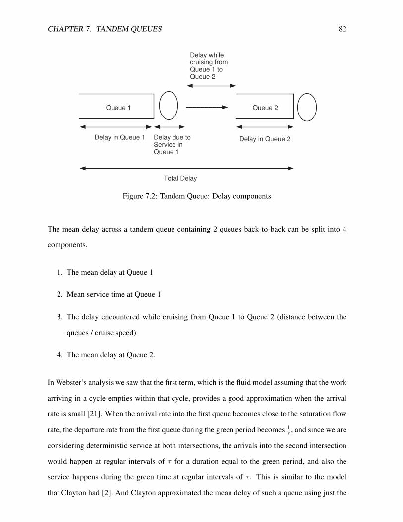
CHAPTER 7. TANDEM QUEUES 82
Delay in Queue 1
Queue 1
Delay due toService inQueue 1
Delay whilecruising fromQueue 1 toQueue 2
Delay in Queue 2
Queue 2
Total Delay
Figure 7.2: Tandem Queue: Delay components
The mean delay across a tandem queue containing 2 queues back-to-back can be split into 4
components.
1. The mean delay at Queue 1
2. Mean service time at Queue 1
3. The delay encountered while cruising from Queue 1 to Queue 2 (distance between the
queues / cruise speed)
4. The mean delay at Queue 2.
In Webster’s analysis we saw that the first term, which is the fluid model assuming that the work
arriving in a cycle empties within that cycle, provides a good approximation when the arrival
rate is small [21]. When the arrival rate into the first queue becomes close to the saturation flow
rate, the departure rate from the first queue during the green period becomes 1τ, and since we are
considering deterministic service at both intersections, the arrivals into the second intersection
would happen at regular intervals of τ for a duration equal to the green period, and also the
service happens during the green time at regular intervals of τ . This is similar to the model
that Clayton had [2]. And Clayton approximated the mean delay of such a queue using just the
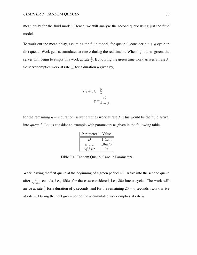
CHAPTER 7. TANDEM QUEUES 83
mean delay for the fluid model. Hence, we will analyse the second queue using just the fluid
model.
To work out the mean delay, assuming the fluid model, for queue 2, consider a r + g cycle in
first queue. Work gets accumulated at rate λ during the red time, r. When light turns green, the
server will begin to empty this work at rate 1τ. But during the green time work arrives at rate λ.
So server empties work at rate 1τ, for a duration y given by,
rλ+ yλ =y
τ
y = rλ1τ− λ
for the remaining g − y duration, server empties work at rate λ. This would be the fluid arrival
into queue 2. Let us consider an example with parameters as given in the following table.
Parameter ValueD 1.5km
vcruise 10m/soffset 0s
Table 7.1: Tandem Queue- Case 1: Parameters
Work leaving the first queue at the beginning of a green period will arrive into the second queue
after Dvcruise
seconds, i.e., 150s, for the case considered, i.e., 30s into a cycle. The work will
arrive at rate 1τ
for a duration of y seconds, and for the remaining 20− y seconds , work arrive
at rate λ. During the next green period the accumulated work empties at rate 1τ.
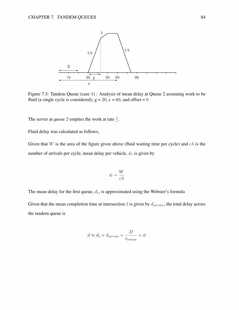
CHAPTER 7. TANDEM QUEUES 84
1/τ
λ
10 80605030
1/τ
y
c
g
Figure 7.3: Tandem Queue (case 1) : Analysis of mean delay at Queue 2 assuming work to befluid (a single cycle is considered); g = 20, c = 60, and offset = 0
The server at queue 2 empties the work at rate 1τ.
Fluid delay was calculated as follows,
Given that W is the area of the figure given above (fluid waiting time per cycle) and cλ is the
number of arrivals per cycle, mean delay per vehicle, w̄, is given by
w̄ = W
cλ
The mean delay for the first queue, d1, is approximated using the Webster’s formula
Given that the mean completion time at intersection 1 is given by dservice, the total delay across
the tandem queue is
d ≈ d1 + dservice + D
vcruise+ w̄
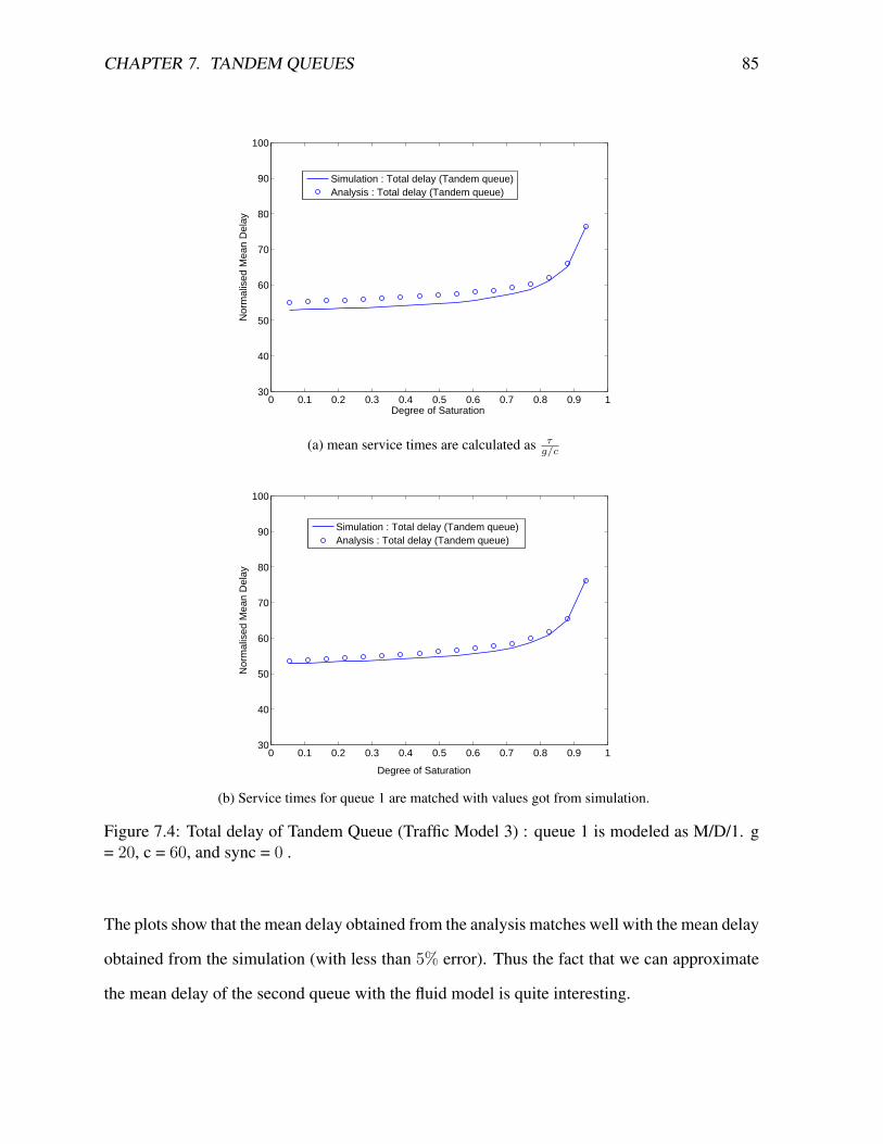
CHAPTER 7. TANDEM QUEUES 85
0 0.1 0.2 0.3 0.4 0.5 0.6 0.7 0.8 0.9 130
40
50
60
70
80
90
100
Degree of Saturation
Nor
mal
ised
Mea
n D
elay
Simulation : Total delay (Tandem queue)Analysis : Total delay (Tandem queue)
(a) mean service times are calculated as τg/c
0 0.1 0.2 0.3 0.4 0.5 0.6 0.7 0.8 0.9 130
40
50
60
70
80
90
100
Degree of Saturation
Nor
mal
ised
Mea
n D
elay
Simulation : Total delay (Tandem queue) Analysis : Total delay (Tandem queue)
(b) Service times for queue 1 are matched with values got from simulation.
Figure 7.4: Total delay of Tandem Queue (Traffic Model 3) : queue 1 is modeled as M/D/1. g= 20, c = 60, and sync = 0 .
The plots show that the mean delay obtained from the analysis matches well with the mean delay
obtained from the simulation (with less than 5% error). Thus the fact that we can approximate
the mean delay of the second queue with the fluid model is quite interesting.

Chapter 8
Extending Modeling and Analysis to
Motorcycle Traffic
In the previous chapters we have modelled and analysed signalised traffic intersections where
vehicles wait in the queue one behind the other. But in developing countries like India a huge
proportion of the traffic is made of 2 wheelers which rarely stand behind a vehicle on arriving
at an intersection. 2 wheelers tend to penetrate the queue and batch up with other vehicles types
whenever it finds free spaces. Hence it is becomes necessary to look at heterogenous traffic, if
we are to find models for accurate estimation of mean delays at intersections serving such kind
of traffic.
8.1 Motorcycles at a Signalized intersection
In chapter [3] we discussed the modeling of queues at an intersection. In this section we would
extend the model to include motorcycle traffic (2 wheelers). Separate attention is required for
the modeling of motorcycles, because motorcycles at an intersection behaves quite different to
how larger vehicles behave. Motorcycles arriving into a queue can find its way through the free
spaces left between larger vehicles and finally settle at a position more closer to the stop line
86
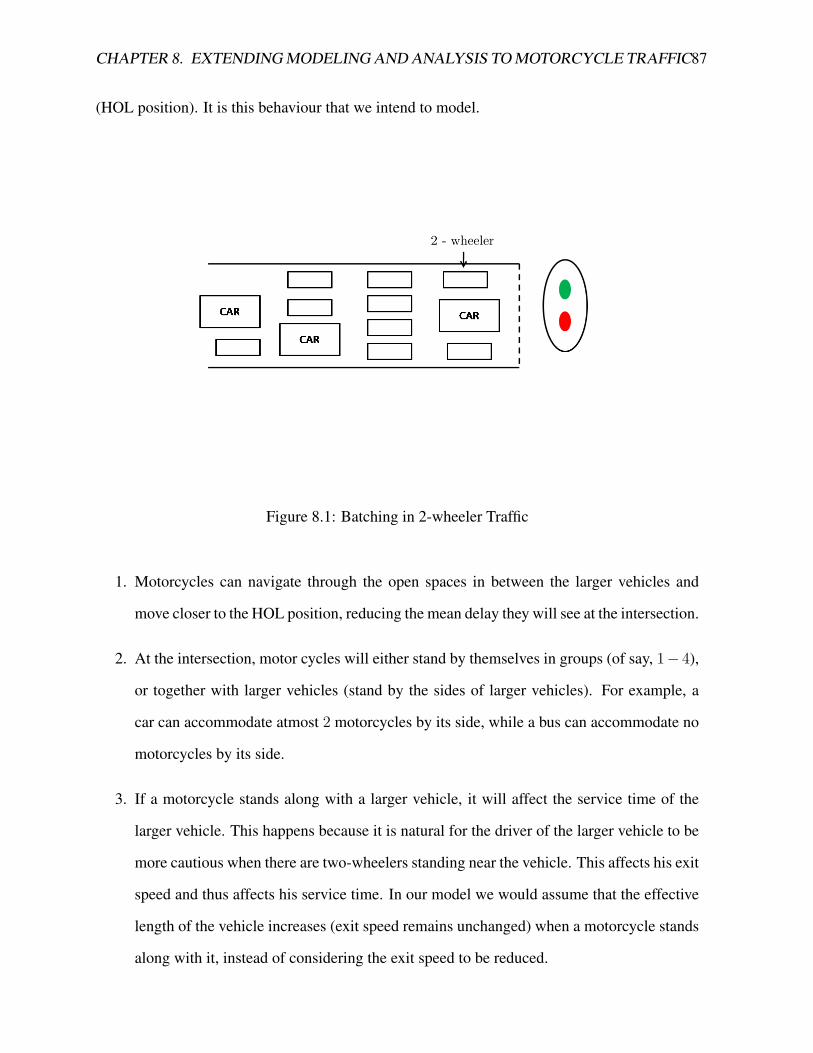
CHAPTER 8. EXTENDING MODELING AND ANALYSIS TO MOTORCYCLE TRAFFIC87
(HOL position). It is this behaviour that we intend to model.
Figure 8.1: Batching in 2-wheeler Traffic
1. Motorcycles can navigate through the open spaces in between the larger vehicles and
move closer to the HOL position, reducing the mean delay they will see at the intersection.
2. At the intersection, motor cycles will either stand by themselves in groups (of say, 1− 4),
or together with larger vehicles (stand by the sides of larger vehicles). For example, a
car can accommodate atmost 2 motorcycles by its side, while a bus can accommodate no
motorcycles by its side.
3. If a motorcycle stands along with a larger vehicle, it will affect the service time of the
larger vehicle. This happens because it is natural for the driver of the larger vehicle to be
more cautious when there are two-wheelers standing near the vehicle. This affects his exit
speed and thus affects his service time. In our model we would assume that the effective
length of the vehicle increases (exit speed remains unchanged) when a motorcycle stands
along with it, instead of considering the exit speed to be reduced.

CHAPTER 8. EXTENDING MODELING AND ANALYSIS TO MOTORCYCLE TRAFFIC88
4. Larger vehicles, though they do not allow motorcycles to stand by their side, would allow
the motorcycles to pass through their sides to occupy vacant spaces in the front.
Comparison between traffic containing 2 wheelers which allows batching
and does not allow batching
We compare a model which does not allow batching of 2 wheelers (2 wheeler arrivals stand at
the back of the queue instead of penetrating the queue) and a model that allows for 2 wheelers
to batch with other vehicle types, to see how the mean delay for a given arrival rate changes
when 2 wheeler batching occurs.
Parameters Traffic Model - MC Traffic Model - MC (2)V {m, c} {m, c}
{lm, lc} {2m, 6m} {2m, 6m}{ dmm(2) , dmm(4) ,dmc(0) , dmc(2) ,dcm(2) , dcm(4) ,dcc(0) , dcc(2)}
{ 2.5m, 3m,7m, 8.5m,3m, 3.5m,8m, 9.5m}
{2.5m, 3.5m,7m, 9.5m,3m, 4m,
8m, 10.5m}{fmm, fmc, fcm, fcc} {0.7, 0.3, 0.6, 0.4} {0.7, 0.3, 0.6, 0.4}
{πm, πc} {0.667, 0.333} {0.667, 0.333}
Table 8.1: Parameters used for traffic flow containing motorcycles. The difference betweenTraffic Model - MC and Traffic Model - MC (2) is that in MC(2) we increase the service timeto allow for decrease in exit speed due to batching.
X-axis Degree of Saturation = λτg/c
; where τ is the mean service time of the FCFS queue
(queue with no batching) of Traffic Model - MC .
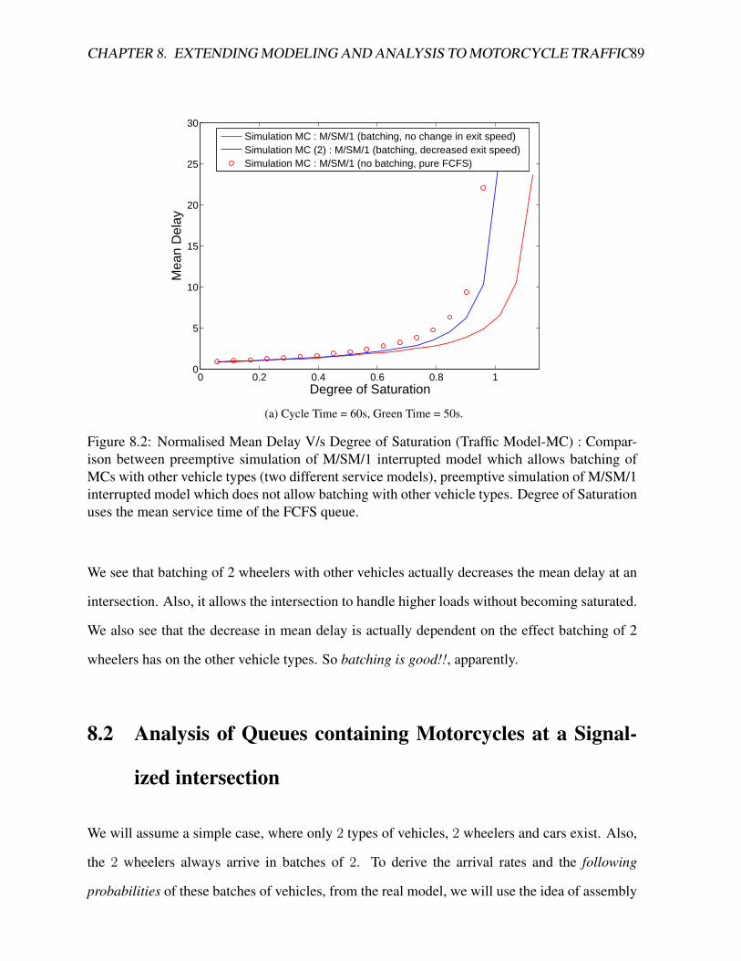
CHAPTER 8. EXTENDING MODELING AND ANALYSIS TO MOTORCYCLE TRAFFIC89
0 0.2 0.4 0.6 0.8 10
5
10
15
20
25
30
Degree of Saturation
Mea
n D
elay
Simulation MC : M/SM/1 (batching, no change in exit speed) Simulation MC (2) : M/SM/1 (batching, decreased exit speed) Simulation MC : M/SM/1 (no batching, pure FCFS)
(a) Cycle Time = 60s, Green Time = 50s.
Figure 8.2: Normalised Mean Delay V/s Degree of Saturation (Traffic Model-MC) : Compar-ison between preemptive simulation of M/SM/1 interrupted model which allows batching ofMCs with other vehicle types (two different service models), preemptive simulation of M/SM/1interrupted model which does not allow batching with other vehicle types. Degree of Saturationuses the mean service time of the FCFS queue.
We see that batching of 2 wheelers with other vehicles actually decreases the mean delay at an
intersection. Also, it allows the intersection to handle higher loads without becoming saturated.
We also see that the decrease in mean delay is actually dependent on the effect batching of 2
wheelers has on the other vehicle types. So batching is good!!, apparently.
8.2 Analysis of Queues containing Motorcycles at a Signal-
ized intersection
We will assume a simple case, where only 2 types of vehicles, 2 wheelers and cars exist. Also,
the 2 wheelers always arrive in batches of 2. To derive the arrival rates and the following
probabilities of these batches of vehicles, from the real model, we will use the idea of assembly
CHAPTER 8. EXTENDING MODELING AND ANALYSIS TO MOTORCYCLE TRAFFIC90
queues. Consider the above example of queue comprising of two types of vehicles, car and
motorcycles.

CHAPTER 8. EXTENDING MODELING AND ANALYSIS TO MOTORCYCLE TRAFFIC91
Notation
λ rate of arrivals into the intersection (arrivals per second)
λm rate of motorcycle arrivals into the intersection (arrivals per second)
λc rate of arrival of cars into the intersection (arrivals per second). We assume λm >
λc for the Markov chain to be positive recurrent.
M4 batch of 4 motorcycles
M2 batch of 2 motorcycles
C0 batch comprising of a car alone
C2 batch comprising of a car and two motorcycles
V set of batches of vehicles arriving into the interrupted queue (V={M2,M4, C0, C2})
λi, i ∈ V rate of departure of a batch i from the assembly queue
χ set of states in the Markov chain (χ= { 1′, 0, 1, 2, . . .})
ai(x) rate of departure of batch type i, i ∈ V from state x, x ∈ χ
φj(x) probability that the next departure from the assembly queue is of batch j given that
currently the system is in state x
νx stationary probability that the Markov chain is in state x, x ∈ χ
fij probability that a batch j follows a batch i
qo probability that the interrupted queue is empty
q1 probability that interrupted queue has exactly one vehicle in the system
µ mean service rate of vehicles at the interrupted queue
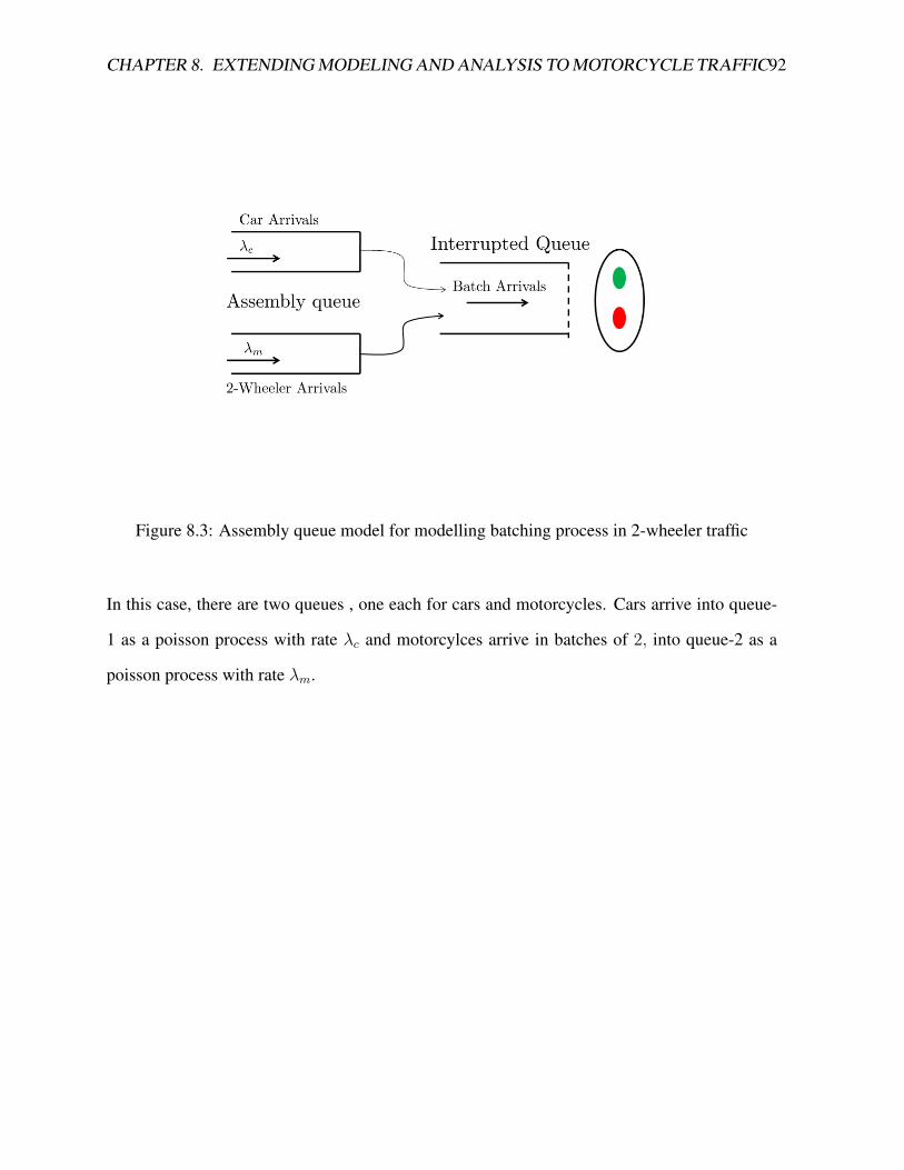
CHAPTER 8. EXTENDING MODELING AND ANALYSIS TO MOTORCYCLE TRAFFIC92
Figure 8.3: Assembly queue model for modelling batching process in 2-wheeler traffic
In this case, there are two queues , one each for cars and motorcycles. Cars arrive into queue-
1 as a poisson process with rate λc and motorcylces arrive in batches of 2, into queue-2 as a
poisson process with rate λm.

CHAPTER 8. EXTENDING MODELING AND ANALYSIS TO MOTORCYCLE TRAFFIC93
Figure 8.4: Markov chain representing the state of the assembly queue.
Consider a Markov chain with possible states {1′, 0, 1, 2, . . . }. Initially when the queues are
empty, the Markov chain is in state 0. Assume that a car arrival occurs next. Now the Markov
chain moves to state 1 if the interrupted queue is non-empty. Assume another car arrival occurs,
causing the Markov chain to move to state 2 (irrespective of whether the interrupted queue is
empty or not). If a motorcycle arrive occurs next, the Markov chain will move to state 1 and a
batch comprising of a car and two motorcycles will depart into the interrupted queue. Similarly
another motorcycle will take the Markov chain to state 0. Now if a motorcycle arrival happens
next and the interrupted queue is non-empty, Markov chain will move to state 1′. Once the
Markov chain is in this state, irrespective of a car arrival or a motorcycle arrival, the Markov
chain will move to state 0, i.e., if the arrival is car, a batch comprising a car and two motorcycles
will leave and if the arrival is of motorcycles, then a batch of 4 motorcycles will depart.
Also, whenever an arrival occur while the Markov chain is in state 0 and the interrupted queue
is empty, the vehicle is immediately released to the interrupted queue. When the Markov chain
is in any state other than 0 and the interrupted queue turns empty, then the vehicle at the head
of the assembly queue will be released to the interrupted queue.
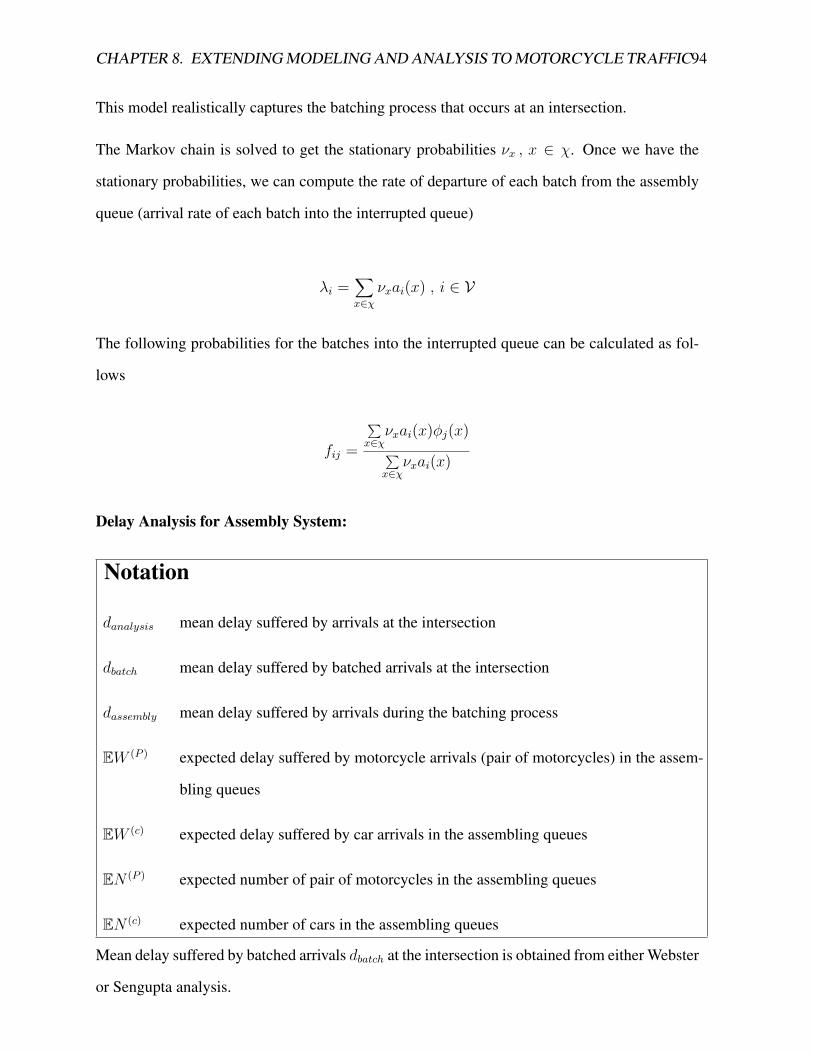
CHAPTER 8. EXTENDING MODELING AND ANALYSIS TO MOTORCYCLE TRAFFIC94
This model realistically captures the batching process that occurs at an intersection.
The Markov chain is solved to get the stationary probabilities νx , x ∈ χ. Once we have the
stationary probabilities, we can compute the rate of departure of each batch from the assembly
queue (arrival rate of each batch into the interrupted queue)
λi =∑x∈χ
νxai(x) , i ∈ V
The following probabilities for the batches into the interrupted queue can be calculated as fol-
lows
fij =
∑x∈χ
νxai(x)φj(x)∑x∈χ
νxai(x)
Delay Analysis for Assembly System:
Notation
danalysis mean delay suffered by arrivals at the intersection
dbatch mean delay suffered by batched arrivals at the intersection
dassembly mean delay suffered by arrivals during the batching process
EW (P ) expected delay suffered by motorcycle arrivals (pair of motorcycles) in the assem-
bling queues
EW (c) expected delay suffered by car arrivals in the assembling queues
EN (P ) expected number of pair of motorcycles in the assembling queues
EN (c) expected number of cars in the assembling queues
Mean delay suffered by batched arrivals dbatch at the intersection is obtained from either Webster
or Sengupta analysis.

CHAPTER 8. EXTENDING MODELING AND ANALYSIS TO MOTORCYCLE TRAFFIC95
Given,
EN (c) =∞∑i=1
iνi
EN (P ) =ν1′
EW (P ) =EN (P )
λm
EW (c) =EN (c)
λc
The mean delay suffered by arrivals during the assembly process (dassembly) can be obtained as
follows.
dassembly = 2λm2λm + λc
EW (P ) + λc2λm + λc
EW (c)
The mean delay suffered by arrivals at the intersection (danalysis) is given by
danalysis = dbatch + dassembly
Fixed Point Iteration Method
We see that once we have computed the following probabilities, then we can use them to com-
pute the mean delay using Webster’s formula and its extensions. But we see that the fij values
depend on q0and q1values and value of µ. And to compute the value of µwe need the fij values.
Thus we would do a fixed point iteration by initially assuming the values of q0,q1,µ and itera-
tively compute the fijvalues required to obtain the mean delay. The question remains as to how
to compute the q0 and q1values for an interrupted queue.

CHAPTER 8. EXTENDING MODELING AND ANALYSIS TO MOTORCYCLE TRAFFIC96
Parameters Traffic Model - MCV {m, c}
{lm, lc} {2m, 6m}{dmm(2) , dmm(4) ,dmc, dmc(2) ,dcm(2) , dcm(4) ,dcc(0) , dcc(2)}
{2.5m, 3m,7m, 8.5m,3m, 3.5m,8m, 9.5m}
{fmm, fmc, fcm, fcc} {0.7, 0.3, 0.6, 0.4}{πm, πc} {0.667, 0.333}
Preceding probability Dist.for m(pmi, i ∈ V)
{0.7, 0.3}
Preceding probability Dist.for c(Pci, i ∈ V)
{0.6, 0.4}
Table 8.2: Parameters used for traffic flow containing motorcycles
Approximation
We use the probabilities that an uninterrupted queue is empty/has exactly one customer, and use
those values for q0 and q1. The results of the analysis done for a preemptive M/SM/1 interrupted
model are given below.

CHAPTER 8. EXTENDING MODELING AND ANALYSIS TO MOTORCYCLE TRAFFIC97
0 0.2 0.4 0.6 0.8 110
20
30
40
50
60
70
80
90
100
110
Degree of Saturation
Mea
n D
elay
(se
cond
s)
Simulation MC : M/SM/1 preemptive interruptionAnalysis MC : Webster M/SM/1Analysis MC : Webster M/SM/1 + assembling delay
(a) Cycle Time = 60s, Green Time = 20s.
0 0.2 0.4 0.6 0.8 10
5
10
15
20
25
30
35
40
Degree of Saturation
Mea
n D
elay
(se
cond
s)
Simulation MC : M/SM/1 preemptive interruptionAnalysis MC : Webster M/SM/1 Analysis MC : Webster M/SM/1 + assembling delay
(b) Cycle Time = 60s, Green Time = 50s.
Figure 8.5: Normalised Mean Delay V/s Degree of Saturation (Traffic Model-MC) : Compari-son between preemptive simulation of M/SM/1 interrupted model, Webster approximation forM/SM/1 interrupted queue with batch arrivals whose service time has been calculated usingfixed point iteration.
We see that the analysis overestimates the delay. There are basically two assumption that we

CHAPTER 8. EXTENDING MODELING AND ANALYSIS TO MOTORCYCLE TRAFFIC98
make in the analysis that could be the reason for this over estimation, 1) we assumes the arrival
of batches into the interrupted queue to be Poisson, which is actually not true, 2) the q0 and q1
values that we use are actually from the analysis for the uninterrupted queue.
To identify which of these assumptions are causing the overestimation, we used the analysis to
compute the mean delay in an untinterrupted queue instead of an interrupted queue. Now the
second assumption becomes true. The results are given below.
X-axis Degree of Saturation = λτg/c
; where τ is the mean service time of the FCFS queue
(queue with no batching) of Traffic Model - MC .

CHAPTER 8. EXTENDING MODELING AND ANALYSIS TO MOTORCYCLE TRAFFIC99
0 0.2 0.4 0.6 0.8 10
1
2
3
4
5
6
7
Degree of Saturation
Mea
n D
elay
(se
cond
s)
Simulation MC : M/SM/1 uninterrupted Analysis MC : Webster M/SM/1
(a) Percentage of 2-wheelers = 80%.
0 0.1 0.2 0.3 0.4 0.5 0.6 0.70
1
2
3
4
5
6
7
8
Degree of Saturation
Mea
n D
elay
(se
cond
s)
Simulation MC : M/SM/1 uninterruptedAnalysis MC : Webster M/SM/1
(b) Percentage of 2-wheelers = 50%
Figure 8.6: Normalised Mean Delay V/s Degree of Saturation (Traffic Model-MC) : Com-parison between simulation of M/SM/1 uninterrupted model, and Webster approximation forM/SM/1 uninterrupted queue with batch arrivals whose service time has been calculated usingfixed point iteration.

CHAPTER 8. EXTENDING MODELING AND ANALYSIS TO MOTORCYCLE TRAFFIC100
0 0.1 0.2 0.3 0.4 0.5 0.6 0.70
5
10
15
20
25
Degree of Saturation
Mea
n D
elay
(se
cond
s)
Simulation MC : M/SM/1 uninterruptedAnalysis MC : Webster M/SM/1
(a) Percentage of 2-wheelers = 4%.
0 0.1 0.2 0.3 0.4 0.5 0.6 0.70
5
10
15
20
25
30
35
Degree of Saturation
Mea
n D
elay
(se
cond
s)
Simulation MC : M/SM/1 uninterruptedAnalysis MC : Webster M/SM/1
(b) Percentage of 2-wheelers = 0.4%
Figure 8.7: Normalised Mean Delay V/s Degree of Saturation (Traffic Model-MC) : Com-parison between simulation of M/SM/1 uninterrupted model, and Webster approximation forM/SM/1 uninterrupted queue with batch arrivals whose service time has been calculated usingfixed point iteration.
From figure [8.6a] we see that the delay from analysis is still an over estimate. As the percentage
CHAPTER 8. EXTENDING MODELING AND ANALYSIS TO MOTORCYCLE TRAFFIC101
of 2 wheelers decrease, the amount of batching also decreases. Figure [8.7b] shows the mean
delay comparison for extremely low percentage of 2-wheelers. Here Poisson arrivals is a very
reasonable approximation for the arrivals into the interrupted queue (due to low percentage of
batching). And we see that the Webster approximation works really well in that case. So we
must assume that analysis over estimates the mean delay because of the assumptions that arrivals
into interrupted queue are Poisson and estimating q0 and q1 using the uninterrupted queue.

Chapter 9
Future Work
We have thus modelled a traffic intersection by using a Poisson process to model the arrival
process and using the car following model for the service process. We have also analysed dif-
ferent models of intersection depending on the service distribution used at the intersection, and
have found approximations for each of those models. We would look to enhance the analytical
model for 2-wheeler traffic to remove the over estimation that is occuring while computing the
mean delay. Extending the analysis of tandem queue model to accurately estimate the mean
delays for different values of offset between the green times, needs to be looked at. Since we
have found that batching reduces the mean delay for a given arrival rate, it would be interesting
to see if we could optimize the green times so that the saturation thoughput at the intersection
is maximised for a given delay bound. We would also like to look at techniques like mobile
sensing and crowd sensing, to see if we could estimate the traffic at an intersection and thus
provide an accurate estimation of delay a vehicle could suffer at that intersection.
102

Bibliography
[1] H. M. Alhassan and J. Ben-Edigbe. Evaluation of passenger car equivalent values under
rainfall. International Proceedings of Computer Science & Information Tech, Vol. 26:p6,
March, 2012.
[2] A.J.H. Clayton. Road traffic calculations. Journal of the ICE, Volume 16, Issue 7:247–
264, Jun., 1941.
[3] Richard Cowan. An analysis of the fixed-cycle traffic-light problem. Journal of Applied
Probability, Vol. 18, No. 3:672–683, Sep., 1981.
[4] J.N. Darroch. On the traffic-light queue. Ann. Math. Statist, Vol. 35, No. 1:380–388, 1964.
[5] Federgruen and Green. Queueing systems with service interruptions. Operations Re-
search, Vol. 34, No. 5:pp. 752–768, Sep. - Oct., 1986.
[6] W. Kraemer and M. Langenbach-Belz. Approximate formulae for the delay in the queuing
system gi/g/1. Congressbook, 8th Internat. Teletraffic Congress, , Melbourne, 235-1/8.,
1976.
[7] G. Latouche and V. Ramaswamy. Introduction to Matrix Analytic Methods in Stochastic
Modeling. ASA/SIAM Series on Statistics and Applied Probability, 1999.
[8] Bhargab Maitra, P.K. Sikdar, and S.L. Dhingra. Modelling congestion on urban roads
and assessing level of service. Journal of Transportation Engineering, Volume 125, No.
6:508–514, November/December 1999.
103
BIBLIOGRAPHY 104
[9] Adolf D. May. Traffic Flow Fundementals. Prentice Hall, Inc. New Jersey, 1990.
[10] Donald R. McNeil. A solution to the fixed-cycle traffic light problem for compound pois-
son arrivals. Journal of Applied Probability, Vol. 5, No. 3:624–635, Dec., 1968.
[11] Alan J. Miller. Settings for fixed-cycle traffic signals. OR, Vol. 14, No. 4:373–386, Dec.,
1963.
[12] G.F Newell. Approximation methods for queues with application to the fixed-cycle traffic
light. SIAM Review, Vol. 7, No. 2:223–240, Apr., 1965.
[13] K. Ohno. Computational algorithm for a fixed cycle traffic signal and new approximate
expressions for average delay. Transportation Science, Vol. 12, No. 1:29–47, Feb., 1978.
[14] S. Panwai and H. Dia. Comparative evaluation of microscopic car-following behavior.
IEEE Transactions on Intelligent Transportation Systems, Volume 6, Issue 3:314–325,
2005.
[15] Richard W. Rothery. Revised monograph on traffic flow theory, chapter 4 - car following
models. Technical report, Transportation Research Board, October , 2000.
[16] Edmond L. Seguin, Kenneth W. Crowley, and W. D. Zweig. Passenger car equivalents on
urban freeways. Technical report, Washington : U.S. Federal Highway Administration,
Offices of Research and Development, 1982.
[17] Bhaskar. Sengupta. A queue with service interruptions in an alternating random environ-
ment. Operations Research, Volume 38 Issue 2:308–318, Mar-April, 1990.
[18] R. J. Serfling. A class of stochastic point process models for traffic flow. Technical report,
Department of Statistics. Florida State University, Tallahassee, Florida, January, 1970.
[19] R. J. Serfling. Non-poisson models for traffic flow. Technical report, Department of
Statistics. Florida State University, Tallahassee, Florida, March, 1969.
[20] van Leeuwaarden. Delay analysis for the fixed-cycle traffic-light queue. Transportation
Science, Vol. 40, No. 2:189–199, May, 2006.

BIBLIOGRAPHY 105
[21] F.V. Webster. Traffic Signal Settings. Department of Scientific and Industrial Research,
Road Research Technical Paper No. 39, Her Majesty’s Stationary Office, London, Eng-
land, 1958.