Topic 4: Aggregate Demand - Trinity College Dublin · Reading and Lecture Plan Reading 1 SWJ Ch. 17 and Clarida et al. (2000) in the QJE. Plan 1 Aggregate Demand (AD) 2 AD with a

Topic 4: Aggregate Demand

Dudley Cooke

Trinity College Dublin

Dudley Cooke (Trinity College Dublin) Topic 4: Aggregate Demand 1 / 34

Reading and Lecture Plan

Reading

1 SWJ Ch. 17 and Clarida et al. (2000) in the QJE.

Plan

1 Aggregate Demand (AD)

2 AD with a Taylor Rule (Monetary Policy)

3 Empirical Application


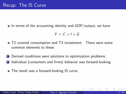
Recap: The IS Curve

In terms of the accounting identity and GDP/output, we have:

Y = C + I + G

T2 covered consumption and T3 investment. There were somecommon elements to these:

1 Derived conditions were solutions to optimization problems.

2 Individual (consumers and firms) behavior was forward-looking.

The result was a forward-looking IS curve.


Aggregate Demand

We can build up a theory of Aggregate Demand (AD) consistent withthis by making some simplifications, whilst keeping the basic insightintact.

Recall,

Y = C + I + G

= C

(Y d

+, r

?, ω0

+

)︸︷︷︸

consn func.

+ I

(Y+

, r−

, K+

)︸︷︷︸

q theory

+ G

Plan is to:

1 Get an expression that is more user-friendly.

2 Add money, i.e. specify what happens in the money market.


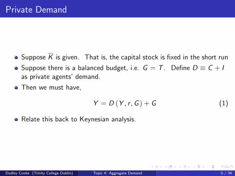
Private Demand

Suppose K is given. That is, the capital stock is fixed in the short run

Suppose there is a balanced budget, i.e. G = T . Define D ≡ C + Ias private agents’ demand.

Then we must have,

Y = D (Y , r , G ) + G (1)

Relate this back to Keynesian analysis.


Transforming Aggregate Demand

Recall, we are interested in both trends and deviations from trend.From (1), AD at trend is simply:

Y = D(Y , r , G

)+ G (2)

Idea (common in macroeconomics): approximate the actual ADaround this trend and then study deviations from the trend, i.e., thebusiness cycle.

The details of this process (i.e. using (1) and (2)) are not crucial forour purposes. In the end, we have the following linear aggregatedemand equation:

y − y = γ1 (g − g)− γ2 (r − r)

where y = ln Y .


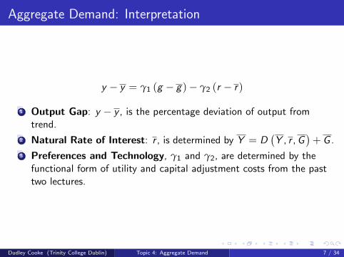
Aggregate Demand: Interpretation

y − y = γ1 (g − g)− γ2 (r − r)

1 Output Gap: y − y , is the percentage deviation of output fromtrend.

2 Natural Rate of Interest: r , is determined by Y = D(Y , r , G

)+ G .

3 Preferences and Technology, γ1 and γ2, are determined by thefunctional form of utility and capital adjustment costs from the pasttwo lectures.


Preferences and Technology, Again

We skipped all the details for the transformation of the AD equation,but they are important [y − y = γ1 (g − g)− γ2 (r − r)] preciselybecause they depend on the assumptions we make regardingpreferences and technology.

In particular, note,

γ1 ≡ m̃ [1− (∂C/∂Y )](G/Y

)> 0

γ2 ≡ −m̃[(∂D/∂r) /Y

]> 0 ; m̃ ≡ 1

1− dD/dY> 0

We know D ≡ C + I = D (Y , r , G ). We are confident dI /dr < 0.But we also know that dC/dr ≷ 0 depends on preferences. However,it seems safe to assume that the joint effect is negative;dD/dr = (dC/dr + dI /dr) < 0. If not, dC/dr would be requiredto be extremely high.1

1The textbook has more on the details of this.Dudley Cooke (Trinity College Dublin) Topic 4: Aggregate Demand 8 / 34

Implications of the AD Equation

If g > g , fiscal policy is above trend. However, changes in g are notlike a simple ‘shift’ in government purchases, as in the IS-LM model.

All else equal, y > y ; that is, output is above trend (which we havecalled the natural rate).

Similarly, when fiscal policy is at trend, but r > r , then y < y ; thatis, output is below trend. Why? Higher r lowers private demand;D ≡ C + I .

Also remember that g is an exogenous policy variable in the model,whereas r is endogenous. We can set g , but r is ‘set for us’ by themodel.


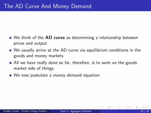
The AD Curve And Money Demand

We think of the AD curve as determining a relationship betweenprices and output.

We usually arrive at the AD curve via equilibrium conditions in thegoods and money markets

All we have really done so far, therefore, is to work on the goodsmarket side of things.

We now postulate a money demand equation


The Money Demand Function

The ‘usual’ assumption about money demand is

M

P= L

(Y+

, i−

)= Y ψ exp (−ρi)

Taking logs,2

⇔ m− p = ψy − ρi

Here, ψ is the income elasticity of money demand and ρ is thesemi-interest elasticity.

If we approximate this, we can use it together with the previousexpression to derive an AD curve.

2Recall that log [exp (x)] = x and ln (1 + x) ' x for small x , used below also.Dudley Cooke (Trinity College Dublin) Topic 4: Aggregate Demand 11 / 34

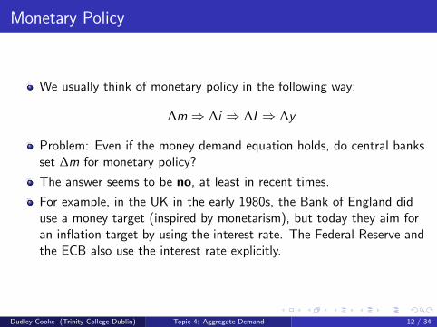
Monetary Policy

We usually think of monetary policy in the following way:

∆m⇒ ∆i ⇒ ∆I ⇒ ∆y

Problem: Even if the money demand equation holds, do central banksset ∆m for monetary policy?

The answer seems to be no, at least in recent times.

For example, in the UK in the early 1980s, the Bank of England diduse a money target (inspired by monetarism), but today they aim foran inflation target by using the interest rate. The Federal Reserve andthe ECB also use the interest rate explicitly.


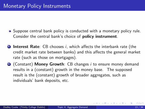
Monetary Policy Instruments

Suppose central bank policy is conducted with a monetary policy rule.Consider the central bank’s choice of policy instrument.

1 Interest Rate: CB chooses i , which affects the interbank rate (thecredit market rate between banks) and this affects the general marketrate (such as those on mortgages).

2 (Constant) Money Growth: CB changes i to ensure money demandresults in a (constant) growth in the money base. The supposedresult is the (constant) growth of broader aggregates, such asindividuals’ bank deposits, etc.


Connecting The Interest Rate To Money Growth

Often, monetary policy is defined in terms of the rate of moneygrowth, not the level of the money supply. We can define the moneygrowth rate as:

M

M−1≡ 1 + µ

Define inflation as:P

P−1≡ 1 + π

Substitute these into the money demand function, in levels:

M−1

P−1= κY ψ exp (−ρi)

1 + π

1 + µ

This is short-run money demand.


Connecting The Interest Rate To Money Growth

In the long run, we have:

Y = Y (output is at trend)

i = r + π (the Fisher equation)

π = µ (inflation is entirely determined by money growth, as in themonetarist approach)

Long-run (i.e. trend) money demand must be:

M−1

P−1= κY

ψexp [−ρ (r + π)]


An Interest Rate Policy

We now use short-run and long-run money demand to find anexpression that accounts for deviations from trend.

In this case,

(1 + µ)(1 + π)

(Y

Y

)ψ

=exp [−ρ (r + π)]

exp (−ρi)

Let’s use a logarithmic transformation, as above.

µ− π + ψ (y − y) = −ρ (r − π) + ρi

We have now connected the output gap, y − y , to the short-termnominal interest rate.


An Interest Rate Policy

Rearranging, we get:

i = r + π +(

1

ρ− 1

)(π − µ) +

ψ

ρ(y − y)

where r and (y − y) are as before.

Three points worth making:

1 corr (i , y − y) > 0. High interest rates are associated with a bigoutput gap.

2 ρ < 1 implies that i increases more than one-for-one with inflation.So via the Fisher equation, r rises. [Taylor Principle.]

3 We can think of µ as an inflation target, a policy that has beenadopted by a number of countries, including the UK. The Eurozone ismore complicated; ‘at or below 2%’ is technically not a target.


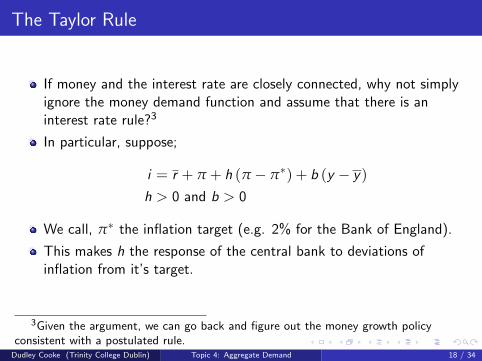
The Taylor Rule

If money and the interest rate are closely connected, why not simplyignore the money demand function and assume that there is aninterest rate rule?3

In particular, suppose;

i = r + π + h (π − π∗) + b (y − y)h > 0 and b > 0

We call, π∗ the inflation target (e.g. 2% for the Bank of England).

This makes h the response of the central bank to deviations ofinflation from it’s target.

3Given the argument, we can go back and figure out the money growth policyconsistent with a postulated rule.


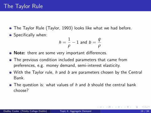
The Taylor Rule

The Taylor Rule (Taylor, 1993) looks like what we had before.

Specifically when:

h =1

ρ− 1 and b =

ψ

ρ

Note: there are some very important differences.

The previous condition included parameters that came frompreferences, e.g. money demand, semi-interest elasticity.

With the Taylor rule, h and b are parameters chosen by the CentralBank.

The question is: what values of h and b should the central bankchoose?


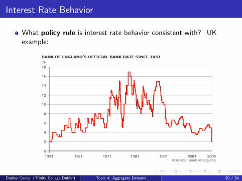
Interest Rate Behavior

What policy rule is interest rate behavior consistent with? UKexample:

Page 1 of 1

18/01/2010http://newsimg.bbc.co.uk/media/images/45268000/gif/_45268583_bank_rates51_08_...


UK Monetary Policy

Consider previous figure:

1 1974: oil price shock

2 Early 1980’s: UK experiments with monetary targeting

3 1987: stock market crash

4 1990-1992: ERM

5 1992: BoE starts targeting inflation

6 1997: BoE independence.


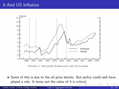
h And US Inflation

2

3

4

5

6

7

8

9

10

11

12

1969 1970 1971 1972 1973 1974 1975 1976 1977 1978 1979

Percent

ForecastActual

Figure 1: Inflation Forecasts and Outcomes

3

4

5

6

7

8

9

10

1969 1970 1971 1972 1973 1974 1975 1976 1977 1978 1979

Percent

ForecastActualu* (Real-Time)u* (Ex-Post)

Figure 2: Unemployment Forecasts and Outcomes

10

Some of this is due to the oil price shocks. But policy could well haveplayed a role. It turns out the value of h is critical.


The Role Of h

Consider the Taylor rule:

i = r + π + h (π − π∗) + b (y − y)

h > 0 is necessary for economic stability. Why? Suppose h < 0: if↑ π, then given i , ↓ (i − π), so ↓ r .

This stimulates consumption and output. AD:

y − y︸︷︷︸higher

= γ1(g − g)︸︷︷︸=0, say

− γ2(r − r)︸︷︷︸<0, say

Higher output leads to greater inflationary pressure (the economy is‘overheating’). This spiral continues. Inflation rises ever higher.


The Role Of h: Countering Inflation

It’s clear that a bad policy will lead to an inflation spiral. Therefore,when inflation rises, the central bank ought to raise nominal interestrates. h > 0.

When this happens, real interest rates increase. This dampensinflation.

Taylor originally suggested b = h = 0.5 as a benchmark.

To ensure that we avoid a vicious cycle, the central bank needs to betough.


Empirical Evidence: The United States, 1960–1996

Clarida et al. (2000) use quarterly time series data for 1960:1–1996:4.They split the sample into pre-Volcker (pre-1979) andVolcker-Greenspan (post-1979) eras.4

They say:

1 “the Federal Reserve was highly accommodative in the pre-Volckeryears ... While it raised the nominal rate, it did so by less than theincrease in expected inflation.”

2 “On the other hand, during the Volcker-Greenspan era the FederalReserve ... systematically raised real as well as nominal short-terminterest rates in response to higher inflation.”

4Paul A. Volcker, Fed Chairman 1979–1987; Alan Greenspan, Fed Chairman1987–2006.


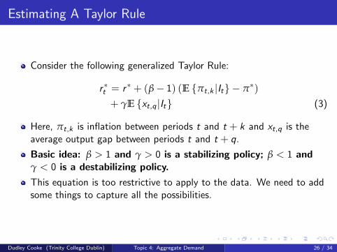
Estimating A Taylor Rule

Consider the following generalized Taylor Rule:

r ∗t = r ∗ + (β− 1) (E {πt,k |It} − π∗)+ γE {xt,q |It} (3)

Here, πt,k is inflation between periods t and t + k and xt,q is theaverage output gap between periods t and t + q.

Basic idea: β > 1 and γ > 0 is a stabilizing policy; β < 1 andγ < 0 is a destabilizing policy.

This equation is too restrictive to apply to the data. We need to addsome things to capture all the possibilities.


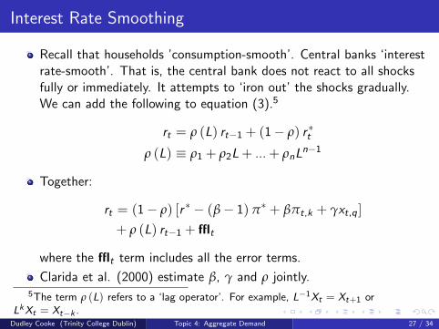
Interest Rate Smoothing

Recall that households ’consumption-smooth’. Central banks ‘interestrate-smooth’. That is, the central bank does not react to all shocksfully or immediately. It attempts to ‘iron out’ the shocks gradually.We can add the following to equation (3).5

rt = ρ (L) rt−1 + (1− ρ) r ∗t

ρ (L) ≡ ρ1 + ρ2L + ... + ρnLn−1

Together:

rt = (1− ρ) [r ∗ − (β− 1) π∗ + βπt,k + γxt,q ]+ ρ (L) rt−1 + fflt

where the fflt term includes all the error terms.

Clarida et al. (2000) estimate β, γ and ρ jointly.5The term ρ (L) refers to a ‘lag operator’. For example, L−1Xt = Xt+1 or

LkXt = Xt−k .Dudley Cooke (Trinity College Dublin) Topic 4: Aggregate Demand 27 / 34

Empirical Evidence: Clarida et al. (2000)

3. Subsample Stability. We next explore the stability ofparameters within each subsample. Among other things, thisexercise permits us to relax the assumption that the in�ationtarget p * is constant within the estimation period. It is conceiv-able, for example, that there was an upward shift in the targetduring the period of rising in�ation in the 1970s.

A simple and natural way to proceed is to assume that thepolicy reaction function is stable during the tenure of the FederalReserve chairman in charge at the time, but may vary acrossChairmen. If we tack the brief period of Miller (78:1–79:3) on toBurns (70:1–78:1), then each subperiod may be divided into tworegimes of roughly equal length. For the pre-1979 sample we thushave Martin (60:1–69:4) and Burns and Miller (70:1–79:2); for thepost-1979 sample Volcker (79:3–87.2) and Greenspan (87.3–96:4).

As discussed earlier, estimating the policy rule over shortsamples can generate imprecise estimates, given the limitednumber of observations. Accordingly, we adopt the followingprocedure: we �rst estimate the reaction function for each base-line period (pre-Volcker or Volcker and Greenspan), but allow for ashift across Chairmen in each of the coefficients (by means ofappropriate dummies). Second, we reestimate the rule afterconstraining all the parameters for which the shift was found tobe insigni�cant in the �rst stage to be constant across Chairmen,while allowing for changes in the remaining parameters. Theresulting estimates are reported in Table V. We present estimates

TABLE IVALTERNATIVE HORIZONS

p* b g r p

k 5 4, q 5 1Pre-Volcker 3.58 0.86 0.34 0.73 0.835

(1.42) (0.05) (0.08) (0.04)Volcker-Greenspan 3.25 2.62 0.83 0.78 0.876

(0.23) (0.31) (0.28) (0.03)k 5 4, q 5 2

Pre-Volcker 3.32 0.88 0.34 0.73 0.833(1.80) (0.06) (0.09) (0.04)

Volcker-Greenspan 3.21 2.73 0.92 0.78 0.886(0.21) (0.34) (0.31) (0.03)

Standard errors are reported in parentheses. The set of instruments includes four lags of in�ation, outputgap, the federal funds rate, the short-long spread, and commodity price in�ation.

MONETARY POLICY RULES 161

β is very different across periods (β is h in our notation). Theestimate of ρ also matters.β increases a lot in the Volcker-Greenspan era. That implies atougher position on increasing real interest rates.


Empirical Evidence: Comments

We could simply conclude that the Fed was too ’weak’ or ’soft’ in the1970’s. However, it isn’t so simple.

Households make consumption choices and firms make investmentchoices based on it , iet+1, iet+2, etc.

By controlling it the bank influences all future iet ’s, i.e., expectationsmatter. This is why we talk about the credibility of a central bankpolicy.


Aggregate Demand: Synthesis

Recall that Aggregate Demand was given by:

y − y = γ1 (g − g)− γ2 (r − r) (4)

We now suppose that the central bank uses the following interest raterule:

i = r + πe1 + h (π − π∗) + b (y − y)

where we have used πe1, not π, in the rule. Using the Fisher

equation,r = r + h (π − π∗) + b (y − y) (5)

Equations (4) and (5) provide the AD curve we use in this course.6

6The central bank will control i , but due to some simplifications we can think of it ascontrolling r directly.


Aggregate Demand: Synthesis

Combining (4) and (5), we have:

y − y = γ (π∗ − π) + D ; γ≡ γ2h

1 + α2b; D≡γ1 (g − g)

1 + γ2b

Where γ gives the slope of the AD curve and D measures (demand)shocks.

1 The sign of h has a very important impact. Notice that h now helpsdetermine the slope of our AD curve.

2 γ1 and γ2 depend on preferences and technology, as stressed earlier.


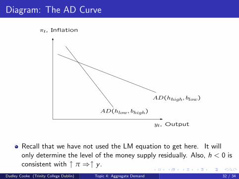
Diagram: The AD CurveDiagram: The AD Curve

πt, Inflation

yt, Output

AD(hlow, bhigh)

AD(hhigh, blow)

Recall that we have not used the LM equation

to get here. It will only determine the level of

the money supply residually.

Recall that we have not used the LM equation to get here. It willonly determine the level of the money supply residually. Also, h < 0 isconsistent with ↑ π ⇒↑ y .


The AD Curve: Comments

This AD has some different properties to the normal AD. Forinstance, y = y (m− p, g , t). However, we can trace things back tomoney demand.

D > 0 when g > g . If government spends more, then the AD shiftsoutwards. If D = 0, then we are at trend.

π∗ also shifts out the AD. Previously, m shifted the AD.

Higher inflation implies that the central bank should raise r , inaccordance with the Taylor principle, which happens when h > 0.


Final Points

Our model depends on rt explicitly via private agents’ behavior.

We have incorporated the idea of the government budget constraintand fiscal policy (the balanced budget condition was also imposed).

We also have some very useful, realistic applicable concepts.

Perhaps the most useful concept for us is the output gap. Thisallows us to think about the inflationary pressures that build up in theeconomy.


Documents

Topic 4: Aggregate Demand - Trinity College Dublin · Reading and Lecture Plan Reading 1 SWJ Ch. 17 and Clarida et al. (2000) in the QJE. Plan 1 Aggregate Demand (AD) 2 AD with a