Tool-Supported Timing Analysis of Automotive

Embedded Systems Master of Science Thesis in Intelligent System Design

MADHUMITA BEHERA

Department of Applied Information Technology

CHALMERS UNIVERSITY OF TECHNOLOGY

Gothenburg, Sweden, 2009

Report No. 2009:065

�

REPORT NO. 2009:065

Tool-Supported Timing Analysis of Automotive Embedded Systems

MADHUMITA BEHERA

Department of Applied Information Technology Chalmers University of Technology

SE-41296, Gothenburg, Sweden 2009

2

Tool-Supported Timing Analysis of Automotive Embedded Systems

MADHUMITA BEHERA

© MADHUMITA BEHERA, 2009

Report no: 2009:065 ISSN: 1651-4769 Address: Department of Applied Information Technology Chalmers University of Technology SE-41296 Gothenburg, Sweden Telephone: Head of Dept: +46 (0)31-786 2763, Information officer: +46 (0)31-786 5548, Student counsellor: +46 (0)31-772 4893 Chalmers Reproservice Göteborg, Sweden 2009

3

SUMMARY:

TIMMO Project aimed to develop a Domain specific Modeling language for handling timing information while developing automotive distributed embedded systems. Hence timing analysis becomes an obvious step in the validation phase of TIMMO results i.e. TADL, the modelling language and TIMMO methodology, guidelines for using this language. To facilitate timing analysis process, a tool survey was conducted followed by tool inventory in order to have a selection of most suitable tools that are currently available for timing analysis. A validator system, basically an automotive embedded system was developed to validate the TIMMO results at Volvo Technology. This validator system was modeled with the timing properties using one of these selected tools. The timing models thus created defined the validator system with timing information associated with it and were analysed to study the behaviour of its timing properties.

A set of structured steps were defined in the form of heuristics to be followed while modeling such

automotive embedded systems along with their timing information. These steps were applied to two different abstraction levels of timing model of the validator system. A timing information flow analysis was also conducted for the different tools involved in defining the validator system in order to find out the possibility of transferring the timing information from one tool to another. By developing a parser in java, it was studied that the timing information defined for modeling an automotive system in one tool can be extracted and can be restructured to model it in another tool.

Keywords:

Automotive, Embedded, Timing Analysis, TIMMO, TADL, Methodology, Validator, Heuristics, Parser

4

Acknowledgement: Foremost, I would like to express my sincere gratitude to my supervisors Andréas Johansson and Claes Strannegård for their motivation, enthusiasm, and guidance through out the process of my thesis work. Their support and encouragement has immensely helped me towards the completion of this thesis. I am grateful to whole TIMMO project team at Volvo Technology whose suggestions and advice has improved my work to a great deal. Finally I would like to thank Mechatronics and Software Department at Volvo Technology for providing me the necessary facilities and technical support during this project.

Madhumita Behera, 2009

5

Contents:

1. Introduction ..................................................................................................................................... 7 1.1. Automotive Embedded System ............................................................................................ 7 1.2. Timing Problems Associated with Automotive Systems ...................................................... 9 1.3. What is a Modeling Language? ........................................................................................... 9 1.4. TIMMO Project ................................................................................................................... 10 1.5. Contributions ...................................................................................................................... 10 1.6. Thesis Structure ................................................................................................................. 11

2. Background ................................................................................................................................... 13 2.1. Modeling Automotive Embedded System .......................................................................... 13

2.1.1. UML ................................................................................................................................ 13 2.1.2. AUTOSAR....................................................................................................................... 13 2.1.3. EAST-ADL2/ATESST (ETAS) ........................................................................................ 13 2.1.4. SysML ............................................................................................................................. 14 2.1.5. MARTE ........................................................................................................................... 15 2.1.6. MATLAB/Simulink ........................................................................................................... 15 2.1.7. AADL (Architecture Analysis & Design Language) ........................................................ 15 2.1.8. Timing Definition Language ............................................................................................ 15 2.1.9. Timed Petri Nets ............................................................................................................. 15 2.1.10. SystemVerilog ................................................................................................................. 16

2.2. Results from TIMMO Project .............................................................................................. 16 2.2.1. TADL ............................................................................................................................... 16 2.2.2. TIMMO Methodology ...................................................................................................... 19

2.3. Validation of TIMMO Results ............................................................................................. 20 2.3.1. Validation Process in TIMMO ......................................................................................... 20 2.3.2. Techniques Used for Timing Analysis ............................................................................ 21

3. Tool Survey and Inventory ........................................................................................................... 23 3.1. Tool Survey for Timing Analysis In TIMMO ....................................................................... 23

3.1.1. List of Surveyed Timing Analysis Tools .......................................................................... 23 3.1.2. Required Tool Properties for Timing Analysis ................................................................ 30 3.1.3. Tool Evaluation with TIMMO Requirements ................................................................... 30 3.1.4. Tool Selection ................................................................................................................. 31

3.2. Tool Inventory .................................................................................................................... 31 3.2.1. Tool Inventory of Task .................................................................................................... 32

4. Information Flow Analysis ........................................................................................................... 37 4.1. Tools Used in TIMMO ........................................................................................................ 37

4.1.1. Volcano VSA: .................................................................................................................. 37 4.1.2. Vector Tools .................................................................................................................... 38 4.1.3. Simulink .......................................................................................................................... 39 4.1.4. SymTA/S ......................................................................................................................... 40

4.2. Information Flow among Tools ........................................................................................... 40 4.2.1. A Parser Development for Information Flow Analysis .................................................... 41 4.2.2. Information flow analysis from VSA to SymTA/S............................................................ 42 4.2.3. Information flow analysis from Vector Tools to SymTA/S .............................................. 43

5. Timing Modeling And Analysis .................................................................................................... 45 5.1. Timing Models using Timing Analysis Tool ........................................................................ 45

5.1.1. Timing Models ................................................................................................................ 45 5.1.2. Schedulability Analysis ................................................................................................... 46

5.2. Example System ................................................................................................................ 47 5.3. Results ............................................................................................................................... 47

5.3.1. Resulted Timing Models ................................................................................................. 47 5.3.2. Results from Timing Analysis ......................................................................................... 49

5.4. Comparative study ............................................................................................................. 52 6. Heuristics For Timing Modeling .................................................................................................. 55

6.1. Heuristics for Design Level & Implementation Level ......................................................... 55

6

6.1.1. Heuristics for Design Level Modeling ............................................................................. 55 6.1.2. Heuristics for Implementation Level Modeling ................................................................ 59 6.1.3. Results from Using Heuristics......................................................................................... 62

7. Analysis Of Results ...................................................................................................................... 63 8. Conclusion ..................................................................................................................................... 64 9. Future Work ................................................................................................................................... 65 10. References ..................................................................................................................................... 66 11. Glossary ......................................................................................................................................... 69

7

1. INTRODUCTION

Behaviour of today’s automotive products is greatly controlled by the embedded electronic systems present in it. These embedded systems are task specific computing or controlling units. These systems are growing in number and complexity with addition of new functionality and features to modern automobiles. Designing and developing such automotive embedded systems requires a structured approach and well defined set of guidelines facilitating this process. Model based approaches have been widely used in automotive industries for managing modeling complexities. Modeling languages are the key to implement such modeling concepts by supporting the process with increased performance and quality. However timing issues has always been a big concern while modeling. Timing is important in almost all real-time embedded systems especially in automotive embedded systems where results of neglecting timing could range from loss of comfort to life threatening situations. Therefore handling timing issues is the most desired feature in a modeling language. Some of the modeling languages that have been successful in modeling engineering systems still face the challenge of handling timing requirements. Hence with existing complexity and need of adding new innovative features in modern automobiles a modeling language should facilitate detecting and handling timing problems early in the process.

1.1. Automotive Embedded System

An embedded system is a computing system which is completely dedicated to perform one or a few more tasks or operations. Such a system is always found embedded inside a complete system. The use of embedded system is growing day by day in many diverse fields. Major application areas are aerospace, automotive, military and medical devices, home appliances etc. The number of fields in which such systems can be used is still growing with new trials and experiments for their use. In future, such systems are expected to be part a major computing and controlling systems because of their flexibility of designing with desired size, cost, safety, reliability features and performance measures. Examples of such system can range from a simple MP3 player to a larger system like nuclear power plant controlling system.

Embedded systems are mostly associated with timing constraints. A very simple example of such

timing constraints faced by an embedded system is a dead-line i.e. a desired time span in which the necessary task of the system has to be completed. Section 1.2 in this chapter brings out some of the timing problems that are faced by these systems. Many such timing problems can arise while carrying out the task or even getting associated with other tasks. Due to the close association with time, these systems are known as real-time embedded systems. For a real-time embedded system not only the correctness of system performance matters but also the timely completion of the task matters. These real-time systems can be categorized mainly into two major categories on the basis of importance of timely completion of the task. These categories are Hard real-time systems and Soft real-time systems. For a Hard real-time system time is the most important factor as the results of missing the dead line could be losing money or even life. Whereas in case of Soft real-time systems missing the dead line of the task may not be hard compared to Hard Real time System. A Flight control system is an example of Hard real-time System, as a single flight error might cause loss of life on the other hand an Airline Reservation System can be cited as an example of a Soft real-time System, since to miss an airline booking is rarely catastrophic.

Embedded Systems have found a great importance in automotive applications as well. A modern

automobile has a number of small and large embedded systems distributed inside it. Anti-lock breaking system (ABS), Navigation System, Emission Control, Climate Control System, Door Control systems are some of the examples of such automotive embedded systems. Most of the automotive embedded systems are hard real- time embedded systems.

8

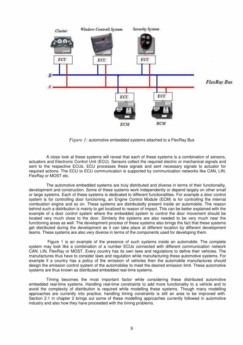
Figure 1: automotive embedded systems attached to a FlexRay Bus

A close look at these systems will reveal that each of these systems is a combination of sensors,

actuators and Electronic Control Unit (ECU). Sensors collect the required electric or mechanical signals and sent to the respective ECUs. ECU processes these signals and sent necessary signals to actuator for required actions. The ECU to ECU communication is supported by communication networks like CAN, LIN, FlexRay or MOST etc.

The automotive embedded systems are truly distributed and diverse in terms of their functionality,

development and construction. Some of these systems work independently or depend largely on other small or large systems. Each of these systems is dedicated to different functionalities. For example a door control system is for controlling door functioning, an Engine Control Module (ECM) is for controlling the internal combustion engine and so on. These systems are distributedly present inside an automobile. The reason behind such a distribution is mainly to get localized to reason of impact. This can be better explained with the example of a door control system where the embedded system to control the door movement should be located very much close to the door. Similarly the systems are also needed to be very much near the functioning areas as well. The development process of these systems also brings the fact that these systems get distributed during the development as it can take place at different location by different development teams. These systems are also very diverse in terms of the components used for developing them.

Figure 1 is an example of the presence of such systems inside an automobile. The complete

system may look like a combination of a number ECUs connected with different communication network CAN, LIN, FlexRay or MOST. Every country has its own laws and regulations to define their vehicles. The manufactures thus have to consider laws and regulation while manufacturing these automotive systems. For example if a country has a policy of the emission of vehicles then the automobile manufactures should design the emission control system of the automobiles to meet the desired emission limit. These automotive systems are thus known as distributed embedded real-time systems.

Timing becomes the most important factor while considering these distributed automotive

embedded real-time systems. Handling real-time constraints to add more functionality to a vehicle and to avoid the complexity of distribution is required while modelling these systems. Though many modelling approaches are currently into practice, handling timing constraints is still an area to be improved with. Section 2.1 in chapter 2 brings out some of these modelling approaches currently followed in automotive industry and also how they have proceeded with the timing problems.

9

1.2. Timing Problems Associated with Automotive Systems

Some of the main timing constraints faced by an embedded real-time systems are deadline,

Worst Case Execution Time, Periodicity, Precedence Constraints, Exclusion Constraint, time offset, jitter and many more. In this section we shall discuss some of these problems

• Deadline: This is the desired time limit for a task execution. In hard real-time system, a task is not at all allowed to exceed a defined time limit or its deadline where as in soft real-time system exceeding execution time limit is not as critical as in a hard real-time system.

• Worst Case Execution Time (WCET): It is the maximum execution time of a task. WCET is one of the timing properties that should be studied in order to have a feasibility study of a system.

• Periodicity: The frequency of task execution within a time span is known as periodicity. Knowledge of periodicity of tasks along with individual execution time helps to find out the total time execution time of a system.

• Precedence Constraints [27]: A task may need to run after another task in order to get the resulted value from it, which is known as a precedence constraint. Precedence constraints are very useful for many types of real-time system: typically we want to implement a `pipeline', where input data is read in to one task, which passes computed results down a pipeline of other tasks and the last task in the chain sending the results to output ports [43].

• Exclusion Constraint: In some cases a task may need to share data or a resource with another task or a number of tasks. So a task has to execute by giving exclusion to other tasks to use the shared resources to another task. This required the control flow to get switched between different tasks. For example let two tasks A and B have access to some shared data structure (such as a linked list). The algorithm that builds the scheduling table must make sure that we never switch to B unless A has completed all its execution, and vice versa these restrictions on how task switch should occur is often called exclusion constraints [43].

Any embedded system or an automotive embedded system to be specific, should satisfy these

timing constraints in order to create a reliable system in terms of safety and performance.

1.3. What is a Modeling Language?

A modeling language is used to express information or knowledge related to a system in a structured way and is defined with a set of rules. It can be graphical or textual. A graphical modeling language uses diagrams and symbols to represent concepts and lines to represent relations whereas a textual modeling language uses standardized keywords and parameters to interpret expressions.

In computer science many modeling languages have emerged. UML (Unified Modeling

Language) [18] could be considered as an example of such languages which has been used for modeling in many diverse fields of expertise and hence is considered as a general purpose modeling language. A generalized modeling language fails to describe a system with its technicalities. To Model an engineering system, a modeling language should be capable of representing various facets of an engineering system. Hence there have been many attempts to develop a modeling language that can be more specific to the desired domain. This resulted into development of some modeling approaches and languages that aimed to completely get adapted to engineering domain requirements.

A considerable amount of effort has been put to develop automotive domain specific modeling

approaches as well. The existing approaches and current achievements for development of automotive embedded system are UML, AUTOSAR (AUTomotive Open System ARchitecture) [3] , AADL [1] and EAST-ADL[12] where as languages for real-time and hardware system are Timed Petri-Nets, Timed Automata, TDL[38], SystemC, SystemVerilog [26], PSL and CTL etc. Such languages tend to support specification, analysis, design, verification and validation of a broad range of systems and systems-of-systems. Along with modeling languages one more modeling approach that is getting very prominent is Meta-Model. For

10

modeling a predefined class of problems, Meta-models have been used in analysis, construction and development of the frames, rules, constraints, models and theories. One of the most active branches of model driven engineering is model-driven architecture proposed by OMG [37] (Object Management Group), which is based on the utilization of a modeling language to write metamodels. This is known as MOF (Meta Object Facility) [25]. Metamodels proposed by OMG are UML, SysML (Systems Modeling Language) [24], SPEM (Software Process Engineering Metamodel) [33] or CWM (Common Warehouse Metamodel) [11].

A special category that has been emerged is Domain-Specific Language which is very specific to

the problems in particular to a domain and does not consider any problem outside it. Domain-specific modeling (DSM) language is engineering system specific language. It can be a considered as a methodology for designing and developing engineering systems. It involves systematic use of a graphical DSL to represent the various facets of a system and supports higher-level abstractions. Hence less effort and fewer low-level details are required to specify a given system. Some these domain specific languages are explained in Section 2.1.

1.4. TIMMO Project

TIMMO (Timing Model) [39] is an ITEA2 Project that started with the joint effort of sixteen

partners from Austria, Germany, France, The Netherland and Sweden in April 2007. TIMMO targets a breakthrough by using a standardized approach for handling such timing related problems. TIMMO aims to develop a modeling language, Timing-Augmented Description Language (TADL) and Methodology for describing the steps to use this language for handling timing problems that may arise in all phases of development of modern automotive systems. Timing-Augmented Description Language as a domain specific modeling language aims to enhance the design models created with any appropriate modeling language by extracting the timing behaviour of the parts of the systems explained by these models.

This thesis project was carried out within the scope of TIMMO aiming at evaluating the suitability of state-of-the-art of the timing analysis tools for automotive embedded systems. The goals of this project is

• To have an early analysis of a system in order to meet the desired timing requirements.

• To trace the timing constraints at all abstraction levels.

• To get improved and predictable development cycle. This project desires for three concrete development results:

• Modeling language: For Timing that enables to model timing aspects where the definition of the language is formalized as a meta-model.

• Methodology: To describe the steps to be followed in different development stages and on the different levels of abstraction with respect to specification, analysis and verification of timing aspect.

• Validation: to verify the applicability of methodology and language by prototype development.

1.5. Contributions This thesis work contributed mainly to the validation of the TIMMO results. The contributions of this

thesis work can be summarized as follows

• A tool survey, as described in Chapter 3 gives a list of academic and commercial tools that can be employed for timing analysis of embedded systems. This list can be useful for any automotive projects that seek information on available tools for timing analysis. The timing behaviour, timing modeling and system feasibility studies are possible using such tools.

11

• Tool inventory, in Chapter 3 gives a list of suitable tools for timing analysis as per TIMMO validator requirements. The methods and analysis processes involved during the selection process, gives an example on how such a selection can be made.

• Timing models developed in timing analysis tools shows how timing analysis can be made at various abstraction levels of an automotive system and how it relates to a generalized development Methodology i.e. TIMMO Methodology. It also helps to analyze the feasibility of a system.

• This thesis presents a heuristics, described in chapter 6 for analysing the timing properties at an early stage while demonstrating it with a real world example i.e. TIMMO Validator developed at Volvo Technology. It shows the feasibility and usefulness of common exchange format across different tools while preventing the re-engineering of models for different purposes. As Heuristics have been applied to two different abstraction level, it helps to give a comparative study of system model. The heuristics from timing model though developed in context of TIMMO validator, can also be applied to other automotive systems.

• An Investigation on the exchange of timing-related information across all tools, used in TIMMO validation process was carried out. A proposed workflow & exchange format to minimize redundant work & speed up interaction was developed. A parser developed for this purpose suggests that exchange of timing information from one tool to another is possible and necessary efforts can be employed to develop a tool to fasten the process of extracting timing information in one tool and then redefining it in another tool. This also application to automotive embedded systems.

1.6. Thesis Structure

This Thesis Report elaborates the validation process of TIMMO methodology and TADL by timing analysis of prototype systems using timing analysis tools. The structure of thesis in short is as followed

• Chapter 2: In this chapter TIMMO results are explained with examples along with validation requirement and validation process:. These results mainly include the TADL, the modeling language and Methodology, steps to use this languages. The employed techniques for timing analysis of TIMMO validators are also described.

• Chapter 3: This chapter mainly contains tool survey for timing analysis. Hence, it contains a list of tools surveyed for timing analysis of automotive embedded systems with their features and limitations. An analysis of the TIMMO validation requirement is made and the surveyed tools are analysed taking the requirements into account. A selection of the tools is made in order to have a selection of most appropriate tools for the timing analysis. As few prototype systems were developed to verify the TIMMO results and the timing analysis of these systems were needed, an analysis of the system requirement was made prior to the timing analysis of these systems. This chapter describes these requirements.

• Chapter 4: An exchange of timing related information among these tools was studied. A sample implementation was made in order to minimize the work and speed up the interaction between tools. Chapter 4 describes this analysis. • Chapter 5: Using some of the tools selected from the tool inventory, timing models were developed for validation and verification of the validator systems. Chapter 5 describes these timing models and gives a comparative study of the results obtained from these models and from the real system.

• Chapter 6: This chapter describes the heuristic develop for creating timing models for two different abstraction levels. These heuristics are list of steps to be followed while developing a timing model of embedded system.

• Chapter 7: It is the summary chapter that summarizes all the work carried out in this thesis project.

12

• Chapter 8: This chapter gives the conclusions drawn from this thesis work

• Chapter 9: This chapter mainly describes future works that can be planned for improving the results.

13

2. BACKGROUND

A number of modeling approaches are currently used for automotive embedded systems. Some of these modeling approaches are general purpose and some of them are very specific to the domain. However handling timing problems has not been a well developed feature in many of these modeling approaches. Considering the timing importance in automotive systems, it is always been a desired feature.

2.1. Modeling Automotive Embedded System

This section lists out some of the currently used modeling approaches in automotive industry and

describes how these approaches have handled the issues faced while handling timing problems. The list is an overview of the modelling approaches described in [41].

2.1.1. UML

UML has long been used as a modeling language in automotive industries. It includes technique

for using graphical notation to create abstract models. UML employed methods specify, visualize and document the facts related to an object-oriented system development. UML can be used throughout the software development life cycle while implementing different technologies. Graphical notations are used by UML to describe a specific system model. Graphical representation includes two main categories 1) Structural Diagram 2) Behavioural diagram. The structural diagram mostly includes class, component, component structure object, package and deployment diagrams, the behavioural diagram include active, behaviour and usecase diagrams.

Though UML can efficiently describe the structure, behaviour and interaction of a system, it has

the draw back of not being very specific to domain and thus fails to define every aspects of system domain. Timing behaviour analysis is something that has never been a concerning matter in UML. To overcome the draw backs of such a generalized modeling language many improved version of UML like SysML has been developed to make it more domain specific.

2.1.2. AUTOSAR

AUTOSAR is a partnership of automotive OEMs, suppliers and tool vendors for creating and

establishing an open standard for automotive system architectures. AUTOSAR aims at providing a basic infrastructure that meets all requirements of automotive application domains. AUTOSAR use a component based software design model for a vehicular system design. It provides a layered architecture that separates the system functionalities from hardware and software components. The basic abstraction layers in AUTOSAR are Basic Software (BSW) Layer, Real Time Environment (RTE) and Application Layer. Basic Software Layer provides the hardware dependent and independent services to the upper layer i.e. the RTE. The RTE acts as a bridge between the software components of the application layer to the respective hardware component of the BSW layer.

However Timing still needs to draw attention in AUTOSAR. Some of the attempts made in order to bring timing feature for software components and connectors were not successful. Approaches on abstract levels also failed [4].

2.1.3. EAST-ADL2/ATESST (ETAS)

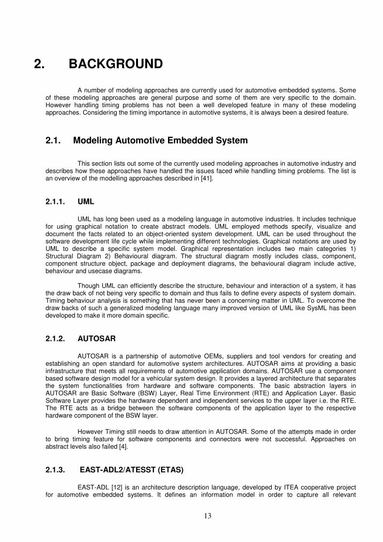
EAST-ADL [12] is an architecture description language, developed by ITEA cooperative project

for automotive embedded systems. It defines an information model in order to capture all relevant

14

engineering information in a standardized way. The language is structured in five abstraction levels as show in Figure 2 below. These abstraction levels reflect different stages of an engineering process.

Figure 2: EAST-ADL Abstraction levels [12]

• Vehicle layer: It describes the features of vehicle.

• Analysis Level: It describes the functional definition of a vehicle.

• Design level: It is mainly concerned with describing the functional features of the vehicle along with the hardware with more details.

• Implementation levels: The hardware and Software components are described in this Implementation level.

• Operational Level: The embedded components are described with all specification in the operational Level.

EAST-ADL2 language supports the modeling requirements by tracing all modeling entities.

EAST_ADL has relevance to AUTOSAR mainly in the implementation level. Timing relevant information is seen as an issue of non-functional requirements and a specialization of quality requirements.

2.1.4. SysML

SysML is an open source project, founded by the SysML Partners. SysML is a Domain-Specific

Modeling language that can support analysis, design, verification and validation of engineering systems [35]. It is defined as a dialect or profile of UML 2.0 and thus can provide mechanisms to collaborate software intensive systems models. It fulfils additional requirements of UML 2.0 with its extended features for reducing the software centric restrictions in UML, supporting tabular notation and features for requirement managements etc.

Being a improved modeling language and a system specific, it also does not include any timing

features like UML 2.0.

15

2.1.5. MARTE

UML continued to be a general purpose modelling language for a long time. It was most obvious

to extend UML to the field of real-time embedded systems by providing more precise expression of domain specific phenomena (e.g., mutual exclusion, concurrency, deadlines etc.). OMG, one of the principal international organizations promoting standards supporting the usage of model-based software and systems development a UML profile named as Schedulability, Performance and Time (SPT). Although SPT could provide concepts for model based schedulability analysis and performance analysis, it could not over come the shortcomings of flexibility and expressiveness. Hence a new UML called MARTE (Modeling and Analysis of Real-Time and Embedded systems) [6] was developed to over come the shortcomings of SPT.

MARTE provides different computational paradigms such as asynchronous, synchronous, and

time. Analysis part in MARTE provides facilities to annotate models with information for model specific analysis, like performance and schedulability analysis.

2.1.6. MATLAB/Simulink

Simulink [32] is an environment for Model-Based Design which can be used for dynamic and

embedded systems with multi-domain simulation and interactive graphical environment. It provides features for designing, simulating, implementing and testing range systems. Its tight integration with MATLAB environment helps to analyze and visualize results and to test data.

Simulink has been considered mainly as a modeling and simulating environment of automotive

embedded systems so far.

2.1.7. AADL (Architecture Analysis & Design Language)

AADL [1] is an architecture modeling notation specifically designed to support modeling of

embedded systems. Its goal is to provide a standard and ways for modeling embedded real-time system architecture with support for analysis and validation of its functional and non-functional properties. It focuses on avionics and automotive domain, where embedded should be able to tolerate faults and guarantee high levels of assurance.

AADL does not contain any mechanisms for specification of timing issues like intervals or dates.

2.1.8. Timing Definition Language

TDL [38] is a programming model for hard real-time systems, thus considered as a Domain

Specific lanagauge. Timing properties of a hard real-time system can be described with its language constructs in a descriptive way. It separates the timing aspect of such applications from the functionality which must be described using an imperative programming language such as Java, C or C++. TDL is concepts are based on Giotto, a time triggered modelling language. The textual notation feature of TADL helps to define the timing behaviours.

2.1.9. Timed Petri Nets

Petri Net is a mathematical modeling language to describe discrete distributed systems. When

Petri net get associated with time it is known as Timed Petri Net [9]. The modeling protocol is by using Petri-Nets. For analysing timing timed automata is used. However not very clear on how it will contribute to timing analysis of automotive systems.

16

2.1.10. SystemVerilog

SystemVerilog [26] is a combined Hardware Description Language (HDL) and Hardware

Verification Language based on extensions to Verilog. Most of the verification functionality is based on the OpenVera language from Synopsys SystemVerilog is based on a behavioural semantics for discrete event simulation comparable to VHDL, SystemC, and SpecC.

Currently timing problems are mostly dealt with late in the development process which is addressed by means of measuring and testing.

2.2. Results from TIMMO Project TIMMO develops a Timing Augmented Descriptive Language (TADL), a modelling language and

methodology for using this language in order to handle timing problems that may arise in all phases of development of modern automotive.

A brief description about these results is given in the following section.

2.2.1. TADL

Following section explains TADL concepts and elements with example. The related work to TADL explained here might have changed. Updated information on TADL and Methodology can be found in TIMMO homepage [39].

2.2.1.1. Concepts involved in TADL

The modeling concept of TADL is based on EAST_ADL2 and AUTOSAR while extending the

structural concepts with time related information. TADL follows the five abstraction levels as described in section 2.1.3 for EAST_ADL. The structural modelling in TADL is performed as defined in EAST-ADL2 mainly on higher abstraction level whereas AUTOSAR modeling is performed on implementation level. The augmentation is done by adding information related to timing and events referring to structural elements [42].

Figure 3: Simplified UML meta-model showing the relationship between events, event chain,

constraints and structural elements in TADL.

17

The TADL constraints are defined being separated from the structural modeling and referring to structural elements via event chains and events, as shown in Figure 3 above. The events are tailored to refer to specific elements in the structural model, i.e. different sets of events are available for the EAST-ADL model and the AUTOSAR model [42].

2.2.1.2. TADL Elements

Event: Any function occurrence that either stimulates an execution, or is caused by an execution is known as an Event. An event is either a Stimulus or a Response (R). An event either indicates that a state change or a current state. Event Chain:

An Event Chains describes the temporal behaviour of a number of steps taken to respond to one or more events. Such events are categorized into stimuli and responses. Time chains can refer to other time chains which are then called time chain segments. Mode:

Modes determine the state of the system, a hardware entity, or an application. The use of modes can be used to filter different views of the model.

ModeGroup:

The set of Modes in a ModeGroup are mutually exclusive. This means that only one Mode of a ModeGroup is active at any point in time. Timing:

Timing is the collection of timing constraints and their descriptions in the form of events and event chains. TimingDescription: It describes the timing events and their relations within the model. TimingConstraint:

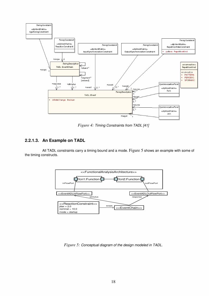
TimingConstraint denotes a requirement entity that allows giving bounds on system timing attributes, i.e., end-to-end delays, periods, etc. Different types of timing constraints described in TADL are 1) AgeTimingConstraint 2) ArbitraryRepetitionConstraint 3) Fork 4) InputSynchronizationConstraint 5) Join 6) OutputSynchronizationConstraint 7) ReactionConstraint 8) RepetitionKind 9) RepetitionRateConstraint 10) SynchronizationPoint [41]. The following Figure 4 shows these timing constraints relating to an event

18

Figure 4: Timing Constraints from TADL [41]

2.2.1.3. An Example on TADL

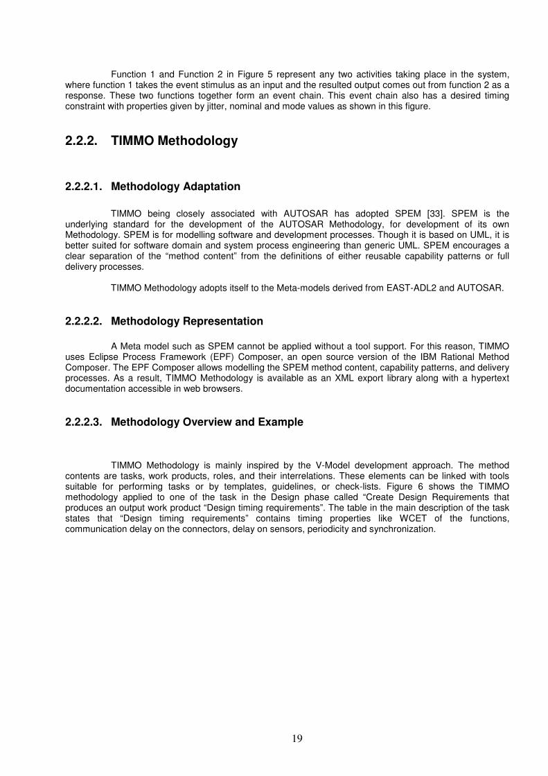
All TADL constraints carry a timing bound and a mode. Figure 5 shows an example with some of

the timing constructs.

<<FunctionalAnalysisArchitecture>>

fcn1:Function

<<EventChain>>

stimulus response

<<ReactionConstraint>>jitter = 2.0nominal = 10.0

mode = startup

scope

<<EventADLInFlowPort>> <<EventADLOutFlowPort>>

inFlowPort outFlowPort

fcn2:Function

Figure 5: Conceptual diagram of the design modeled in TADL.

19

Function 1 and Function 2 in Figure 5 represent any two activities taking place in the system,

where function 1 takes the event stimulus as an input and the resulted output comes out from function 2 as a response. These two functions together form an event chain. This event chain also has a desired timing constraint with properties given by jitter, nominal and mode values as shown in this figure.

2.2.2. TIMMO Methodology

2.2.2.1. Methodology Adaptation

TIMMO being closely associated with AUTOSAR has adopted SPEM [33]. SPEM is the underlying standard for the development of the AUTOSAR Methodology, for development of its own Methodology. SPEM is for modelling software and development processes. Though it is based on UML, it is better suited for software domain and system process engineering than generic UML. SPEM encourages a clear separation of the “method content” from the definitions of either reusable capability patterns or full delivery processes. TIMMO Methodology adopts itself to the Meta-models derived from EAST-ADL2 and AUTOSAR.

2.2.2.2. Methodology Representation

A Meta model such as SPEM cannot be applied without a tool support. For this reason, TIMMO

uses Eclipse Process Framework (EPF) Composer, an open source version of the IBM Rational Method Composer. The EPF Composer allows modelling the SPEM method content, capability patterns, and delivery processes. As a result, TIMMO Methodology is available as an XML export library along with a hypertext documentation accessible in web browsers.

2.2.2.3. Methodology Overview and Example

TIMMO Methodology is mainly inspired by the V-Model development approach. The method

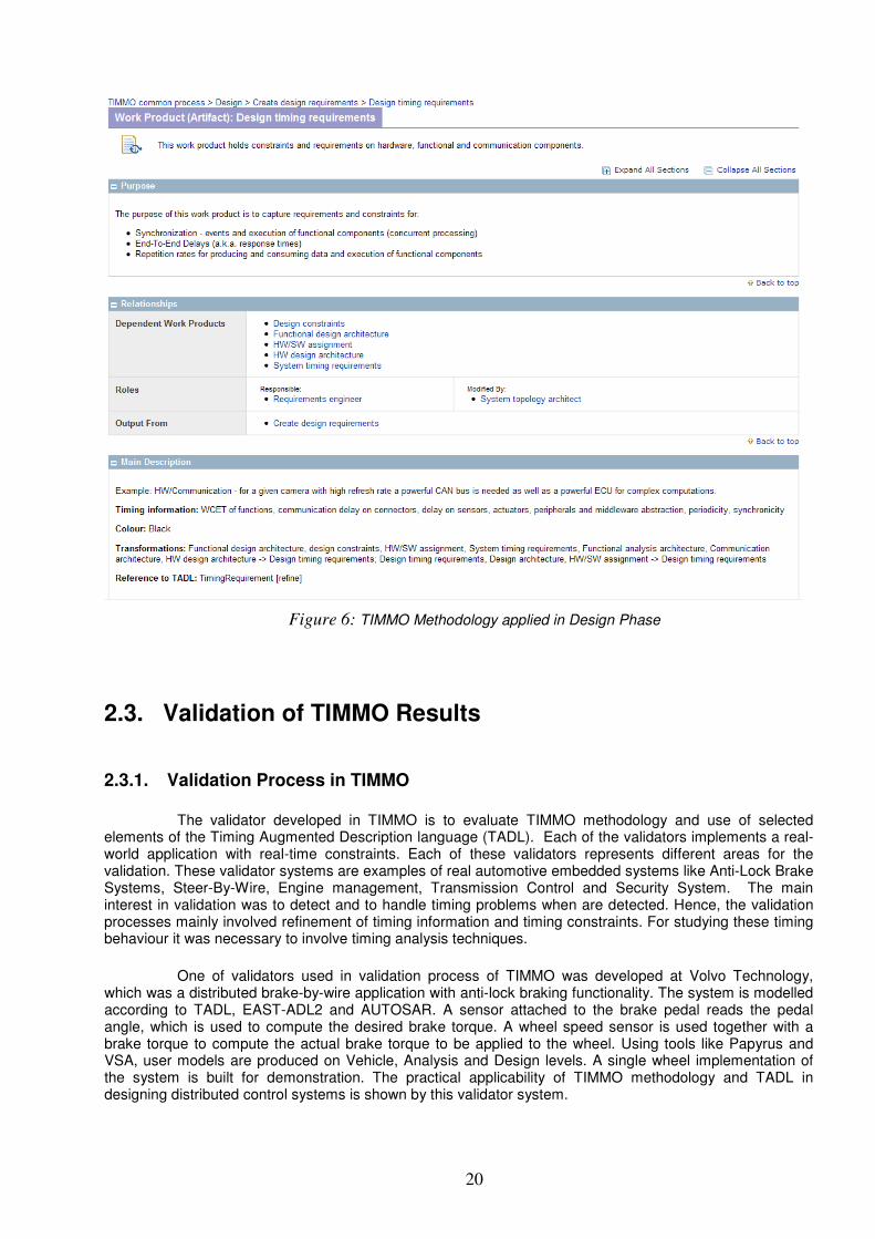
contents are tasks, work products, roles, and their interrelations. These elements can be linked with tools suitable for performing tasks or by templates, guidelines, or check-lists. Figure 6 shows the TIMMO methodology applied to one of the task in the Design phase called “Create Design Requirements that produces an output work product “Design timing requirements”. The table in the main description of the task states that “Design timing requirements” contains timing properties like WCET of the functions, communication delay on the connectors, delay on sensors, periodicity and synchronization.

20

Figure 6: TIMMO Methodology applied in Design Phase

2.3. Validation of TIMMO Results

2.3.1. Validation Process in TIMMO

The validator developed in TIMMO is to evaluate TIMMO methodology and use of selected

elements of the Timing Augmented Description language (TADL). Each of the validators implements a real-world application with real-time constraints. Each of these validators represents different areas for the validation. These validator systems are examples of real automotive embedded systems like Anti-Lock Brake Systems, Steer-By-Wire, Engine management, Transmission Control and Security System. The main interest in validation was to detect and to handle timing problems when are detected. Hence, the validation processes mainly involved refinement of timing information and timing constraints. For studying these timing behaviour it was necessary to involve timing analysis techniques.

One of validators used in validation process of TIMMO was developed at Volvo Technology, which was a distributed brake-by-wire application with anti-lock braking functionality. The system is modelled according to TADL, EAST-ADL2 and AUTOSAR. A sensor attached to the brake pedal reads the pedal angle, which is used to compute the desired brake torque. A wheel speed sensor is used together with a brake torque to compute the actual brake torque to be applied to the wheel. Using tools like Papyrus and VSA, user models are produced on Vehicle, Analysis and Design levels. A single wheel implementation of the system is built for demonstration. The practical applicability of TIMMO methodology and TADL in designing distributed control systems is shown by this validator system.

21

2.3.2. Techniques Used for Timing Analysis

There are different techniques available for timing analysis. Some of these technologies are studied for applying to TIMMO validators. Below is the list some of the timing analysis techniques studied before any timing analysis performed in validation process. Model Checking

Model checking [13] is an automated approach for checking weather a system description (model M) satisfies a given specification. It is mainly applied to hardware design. The system description is given as source code of a hardware descriptive language, which can be modeled by a Finite State Machine (FSM). FSM consists of graphs with nodes representing states of a system. There are two different algorithms for model checking

1. Explicit model checking: it checks the model by building transition system of the given system description and verifies the system using graph search algorithms. 2. Symbolic model checking: It is based on Binary decision diagrams (BDD) for CTL formulas or on SAT solvers.

Scheduling Analysis Scheduling is mainly concerned with assigning time slots to the available computational resources such as processors or hardware/software objects to executable entities (e.g. task) in order to meet the system constraints. Off-line scheduling refers to the scheduling made before the tasks are available on the other hand On-line scheduling refers to a scheduling is generated whiles the tasks are executing. Scheduling is governed by different classes of constraints such as timing constraints (e.g. deadlines, periodicity), precedence constraints (enforced task ordering) and exclusion constraints (while accessing shared objects). Real-Time Queuing Theory

Real-time Queuing Theory (RTQT) [21] provides an approximation method for computing the fraction of tasks that miss their deadlines in systems with high average-case utilization. RTQT takes timing constraints of tasks into account while computing the service times of tasks.

The scheduling policy in RTQT was originally derived from earliest-deadline-first (EDF) policy.

EDF results can be used to provide results for other scheduling policies, like static priority approaches or FIFO. RTQT predicts whether an arriving task will miss its deadline or not in a case the task workload exceeds the mean of the deadline distribution. WCET-Analysis WCET is the maximum time taken by a task or a runnables to execute on a particular CPU. Tasks and runnables are the time consuming elements in any OSEK and AUTOSAR execution models. WCET analysis involves mainly two steps which are program analysis and architecture modeling. Program analysis step analyses the execution path through out the control flow where as Architecture modeling determines the time spend on that path in a particular CPU architecture. WCET analysis [45] is different than other techniques as it does not suggest the feasibility of a system rather the results obtained from this analysis are used as input for schedulability analysis, i.e. for finding out whether a real-time embedded system meets all its timing constraints or not.

22

23

3. TOOL SURVEY AND INVENTORY

One way of doing timing analysis can be by using already existing timing analysis tools that are

build on timing analysis techniques. A survey of such tools available for timing analysis was made. These tools were further analyzed for a selection of appropriate tool set on the basis of their provided automotive support.

3.1. Tool Survey for Timing Analysis In TIMMO

3.1.1. List of Surveyed Timing Analysis Tools

From the survey, tools supporting timing analysis techniques were identified. These tools are

present either as commercial or as free academic tools. These tools can be further divided into two main categories based on their performed levels of timing analysis.

1. Static Method timing analysis tools: Code Level 2. Schedulability analysis tools: System level

Static level timing analysis is based on the code level of the system which basically includes WCET analysis. The broad categorization of timing analysis tools in given in

Figure 7: categorization of timing analysis tools

3.1.1.1. Code Level Timing Analysis

Code level timing analysis mainly includes safe upper bounds computation on WCET of

sequential tasks. These analyses are performed based on static methods for timing analysis which do not rely on executing code on real hardware or on a simulator, rather obtains upper bounds by taking the task codes into account and combining it with some (abstract) model of the system. Static methods include methods like value analysis, Control flow analysis, Process flow analysis, WCET estimation and symbolic simulations etc.

24

3.1.1.1.1. Academic Tools

Heptane: About Heptane [16]:

• Heptane is a timing analysis tool which is licensed under the terms of GNU General Public License (GPL). The software and its source code is licensed free of charge, but any developed version of it should also be released under same GPL licence.

Features:

• It computes WCET by static analysis.

• It is designed to read/write XML files.

• It can analyze C source code while taking into account pipeline and instruction caches. Limitations:

• It only supports microcontrollers of Pentium I, MIPS architecture and Hitachi H8/300.

SymTA/P About SymTA/P [14]:

• SymTA/P Tool from TU Braunschweig, Germany. Features:

• Obtains upper and lower Execution time bounds of C programs running on microcontrollers.

• The longest and shortest paths in the control flow graph are found by Implicit Path Enumeration Technique (IPET).

Limitations:

• The measurement on an evaluation board is more accurate if the program paths between measurements points are longer. If many basic blocks are measured individually, the added time delays to cover pipelining effects would lead to pessimistic WCET.

SWEET

About SWEET [36]:

• It is a prototype tool for WCET analysis developed by the Mälardalen WCET research group

• It is free software, but still a prototype tool (not completely developed as a tool kit).

• Licence is unknown. Features:

• Can handle full ANSI-C programs including pointers, unstructured code, and recursion.

• Integrated with a compiler and performs code flow analysis on the intermediate representation (IR) of the compiler.

• Supports the NECV850E and ARM9 processors.

• Supports three different calculation methods: fast path-based method, global IPET method, and hybrid clustered method.

• Runs on Solaris, Linux and Windows system.

25

calc_wcetC_167: About calc_wcetC_167 [44]:

• It was developed by TU-Vienna (University of Vienna). It is a WCET analysis framework that allows analyzing programs given as C source code (written in wcetC, a special dialect developed for WCET analysis) and also as assembly code.

• Initially developed to analyze code for the C167CR processor from Siemens.

• WCET calculation tool are currently only targeted to the C167CR processor from Siemens.

Features:

• Calculates WCET on code level. WCET-compiler for wcetC provides a WCET analysis framework that interfaces to the user at source code level. Plain assembly files can be analyzed by adding the required path annotations and calling the low-level WCET analysis tool directly.

Limitations:

• At the time of writing this report this tool was under construction.

• Processor specific (currently developed to analyze code for C167CR processor from Siemens).

OTAWA: About OTAWA [2]:

• This tool is from the Traces Research group on Architectures and Compilers for Embedded Systems at IRIT (University of Toulouse, France). It is freely available under the LGPL licence; hence the latter developed version could be released as free or proprietary software. It is a framework of C++ classes dedicated to static analyses of programs in machine code and computation of WCET.

• Used in several research projects 1. MASCOTTE (ANR5), Num@Tec Automotive cluster). 2. MORE (ANR). 3. MERASA (European project)

Features:

• Provides state-of-art WCET analysis like IPET, facilities to work on binary programs (control flow graphs, loop detection and so on).

• Supports architectures like PowerPC, ARM or M68HCS.

Limitations:

• Works only on Linux (Ubuntu). Tu-Bound: About Tu-Bound [14]:

• Developed at Vienna University of Technology.

• No information on license.

Features:

• Tool for worst-case execution time (WCET) analysis of C++ programs.

• Allows high-level annotations to be placed at the source code and has support for static analysis.

• User interface to support the timing analysis with domain-specific knowledge.

26

• A textual intermediate representation for automatically generated results generated by the static program analysis component.

Limitations:

• At the time writing this thesis this tool was not a completely developed as a tool set for timing analysis still a conceptual one.

Chronos About Chronos [10]:

• Developed by The Chronos Research Prototype from National University of Singapore.

• Released under GNU GPL and hence a freely available software. Features:

• Supports the analysis of (i) out-of-order pipelines, (ii) various dynamic branch prediction schemes, (iii) Instruction caches, and the interaction among these different features to compute a tight upper bound on the execution times.

Limitations:

• Does not analyze data caches.

• Performs limited data flow analysis to compute loop bounds.

3.1.1.1.2. Commercial Tools

aiT: About aiT [5]:

• A commercial tool developed by AbsInt GmbH.

• It has WCET Analyzers to compute WCET bounds of tasks in real-time systems.

• Directly analyzes binary executables and takes the intrinsic cache and pipeline behaviour into account.

Features:

• Analyzes binary executables.

• Independent of the compiler and source code language used.

• aiT supports integration with state-of-the-art development tools like SCADE Suite, ASCET, SymTA/S, WCC, RT-Druid, Limitations:

• Evaluation versions of aiT are available for the following processor combinations: ARM7, HCS12/STAR12, PowerPC 555/565/755, C16x/ST10, TMS320C3x, TriCore 1796

BoundT: About BoundT [7]:

• Space Systems Finland Ltd (SSF) developed Bound-T at first for the European Space Agency and used it in space projects. Tidorum Ltd is now making Bound-T commercially available.

27

Features:

• BoundT computes bounds on execution time, bounds on stack usage, Control flow graphs and call trees, bounds on counter-type loops.

• Static analysis of machine code covers all cases.

• Context-sensitive: loop-bounds can use parameters.

• Independent of programming language.

Limitations:

• Bound-T execution-time analyzer has been adapted to the following target processors: Intel-8051 Series, SPARC V7, Analog Devices ADSP-21020

RapiTime: About RapiTime [29]:

• A commercial tool developed by Rapita Systems.

• A software toolkit that provides solution to the problem of worst-case execution time analysis and performance profiling, a solution that works for complex software running on advanced embedded microprocessors.

Features:

• RapiTime supports automatic instrumentation on target testing and execution, Hardware traces capture, Code coverage analysis, Performance profiling.

• It also supports WCET analysis: 1).Determines WCET. 2) Visualizes the contribution of each function to the overall worst-case 3) Examines worst-case execution frequencies 4) Identifies code on the worst-case path 5) Explores the variability in execution times due to hardware effects.

• Targeted optimisation.

• Support for C and Ada.

3.1.1.2. System Level Timing Analysis

System level timing-analysis is done by executing task sets on the given hardware or a simulator

with given set of inputs, and measuring the execution time of the tasks. This mainly includes approaches for End-to-end measurements of a subset of all possible executions, measure the execution times of code segments, typically of CFG (Control flow graphs) basic blocks, bound calculation, to produce estimates of the WCET or BCET, schedulability of task set.

The measurements made in static methods can be necessary inputs for system level analysis.

3.1.1.2.1. Academic Tools

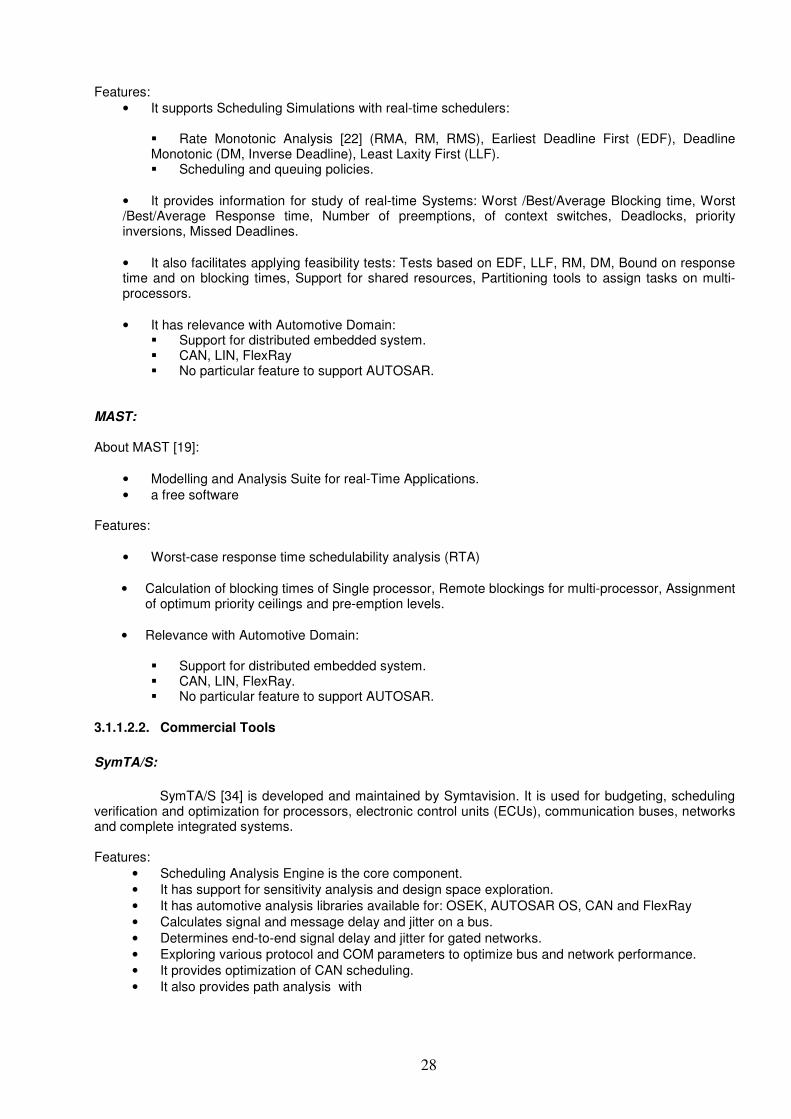
Cheddar About Cheddar [46]:

Cheddar is developed and maintained by LISyC Team, University of Brest. It is written in Ada. Graphical editor is made with GtkAda. It runs on win32 boxes, Solaris, Linux. Cheddar is a free real-time Scheduling tool that analyzes systems in AADL [1] or any Cheddar specific languages.

28

Features:

• It supports Scheduling Simulations with real-time schedulers:

� Rate Monotonic Analysis [22] (RMA, RM, RMS), Earliest Deadline First (EDF), Deadline Monotonic (DM, Inverse Deadline), Least Laxity First (LLF). � Scheduling and queuing policies.

• It provides information for study of real-time Systems: Worst /Best/Average Blocking time, Worst /Best/Average Response time, Number of preemptions, of context switches, Deadlocks, priority inversions, Missed Deadlines.

• It also facilitates applying feasibility tests: Tests based on EDF, LLF, RM, DM, Bound on response time and on blocking times, Support for shared resources, Partitioning tools to assign tasks on multi-processors.

• It has relevance with Automotive Domain: � Support for distributed embedded system. � CAN, LIN, FlexRay � No particular feature to support AUTOSAR.

MAST: About MAST [19]:

• Modelling and Analysis Suite for real-Time Applications.

• a free software

Features:

• Worst-case response time schedulability analysis (RTA)

• Calculation of blocking times of Single processor, Remote blockings for multi-processor, Assignment of optimum priority ceilings and pre-emption levels.

• Relevance with Automotive Domain:

� Support for distributed embedded system. � CAN, LIN, FlexRay. � No particular feature to support AUTOSAR.

3.1.1.2.2. Commercial Tools

SymTA/S:

SymTA/S [34] is developed and maintained by Symtavision. It is used for budgeting, scheduling verification and optimization for processors, electronic control units (ECUs), communication buses, networks and complete integrated systems. Features:

• Scheduling Analysis Engine is the core component.

• It has support for sensitivity analysis and design space exploration.

• It has automotive analysis libraries available for: OSEK, AUTOSAR OS, CAN and FlexRay

• Calculates signal and message delay and jitter on a bus.

• Determines end-to-end signal delay and jitter for gated networks.

• Exploring various protocol and COM parameters to optimize bus and network performance.

• It provides optimization of CAN scheduling.

• It also provides path analysis with

29

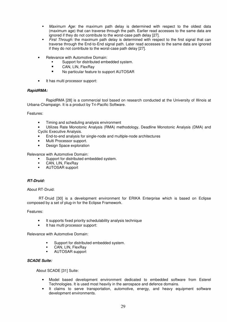
� Maximum Age: the maximum path delay is determined with respect to the oldest data (maximum age) that can traverse through the path. Earlier read accesses to the same data are ignored if they do not contribute to the worst-case path delay [27].

� First Through: the maximum path delay is determined with respect to the first signal that can traverse through the End-to-End signal path. Later read accesses to the same data are ignored if they do not contribute to the worst-case path delay [27].

• Relevance with Automotive Domain: � Support for distributed embedded system.

� CAN, LIN, FlexRay � No particular feature to support AUTOSAR

• It has multi processor support:

RapidRMA:

RapidRMA [28] is a commercial tool based on research conducted at the University of Illinois at

Urbana-Champaign. It is a product by Tri-Pacific Software. Features:

• Timing and scheduling analysis environment

• Utilizes Rate Monotonic Analysis (RMA) methodology, Deadline Monotonic Analysis (DMA) and Cyclic Executive Analysis.

• End-to-end analysis for single-node and multiple-node architectures

• Multi Processor support.

• Design Space exploration

Relevance with Automotive Domain: � Support for distributed embedded system. � CAN, LIN, FlexRay � AUTOSAR support

RT-Druid: About RT-Druid: RT-Druid [30] is a development environment for ERIKA Enterprise which is based on Eclipse composed by a set of plug-in for the Eclipse Framework. Features:

• It supports fixed priority schedulability analysis technique

• It has multi processor support: Relevance with Automotive Domain:

� Support for distributed embedded system. � CAN, LIN, FlexRay � AUTOSAR support

SCADE Suite:

About SCADE [31] Suite:

• Model based development environment dedicated to embedded software from Esterel Technologies. It is used most heavily in the aerospace and defence domains.

• It claims to serve transportation, automotive, energy, and heavy equipment software development environments.

30

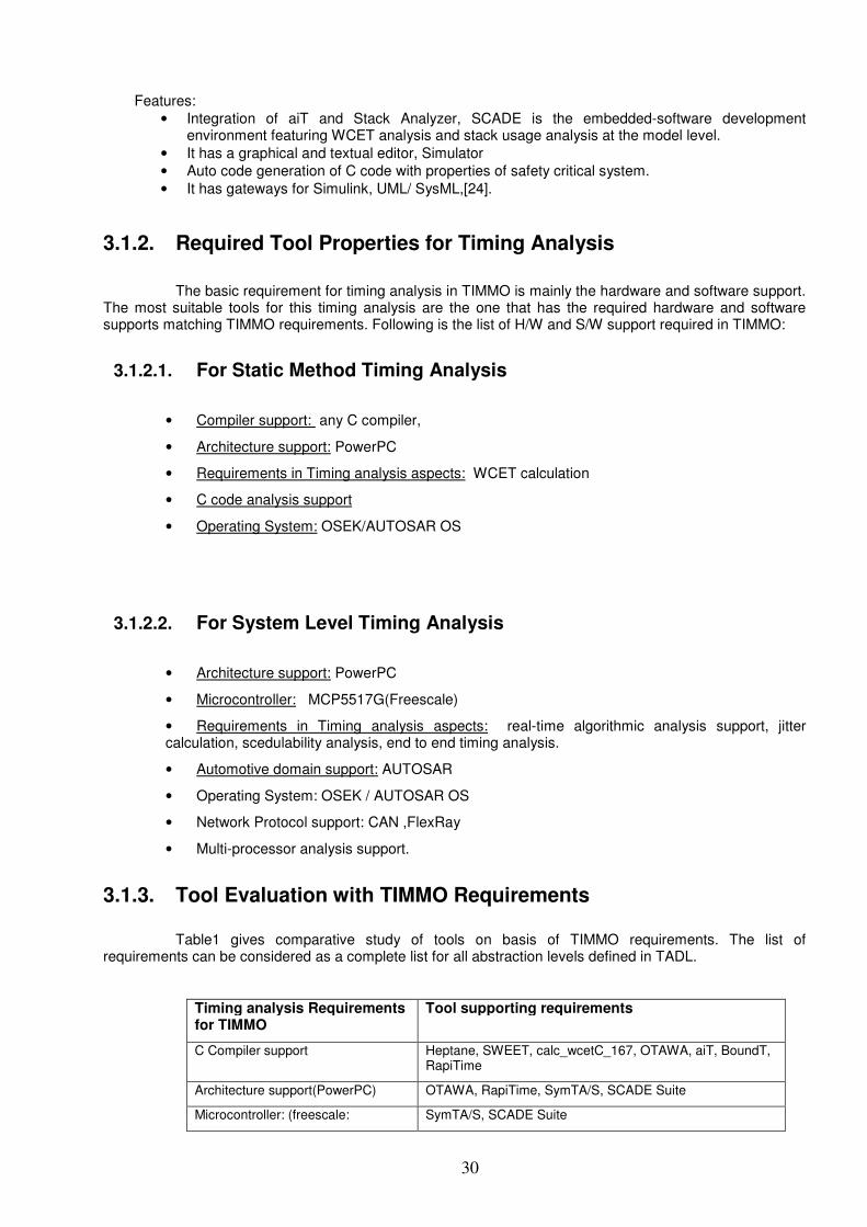
Features:

• Integration of aiT and Stack Analyzer, SCADE is the embedded-software development environment featuring WCET analysis and stack usage analysis at the model level.

• It has a graphical and textual editor, Simulator

• Auto code generation of C code with properties of safety critical system.

• It has gateways for Simulink, UML/ SysML,[24].

3.1.2. Required Tool Properties for Timing Analysis

The basic requirement for timing analysis in TIMMO is mainly the hardware and software support.

The most suitable tools for this timing analysis are the one that has the required hardware and software supports matching TIMMO requirements. Following is the list of H/W and S/W support required in TIMMO:

3.1.2.1. For Static Method Timing Analysis

• Compiler support: any C compiler,

• Architecture support: PowerPC

• Requirements in Timing analysis aspects: WCET calculation

• C code analysis support

• Operating System: OSEK/AUTOSAR OS

3.1.2.2. For System Level Timing Analysis

• Architecture support: PowerPC

• Microcontroller: MCP5517G(Freescale)

• Requirements in Timing analysis aspects: real-time algorithmic analysis support, jitter calculation, scedulability analysis, end to end timing analysis.

• Automotive domain support: AUTOSAR

• Operating System: OSEK / AUTOSAR OS

• Network Protocol support: CAN ,FlexRay

• Multi-processor analysis support.

3.1.3. Tool Evaluation with TIMMO Requirements

Table1 gives comparative study of tools on basis of TIMMO requirements. The list of

requirements can be considered as a complete list for all abstraction levels defined in TADL.

Timing analysis Requirements for TIMMO

Tool supporting requirements

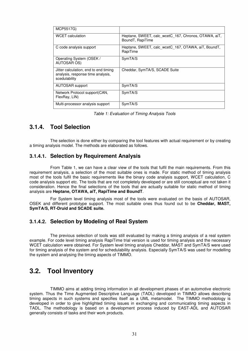
C Compiler support Heptane, SWEET, calc_wcetC_167, OTAWA, aiT, BoundT, RapiTime

Architecture support(PowerPC) OTAWA, RapiTime, SymTA/S, SCADE Suite

Microcontroller: (freescale: SymTA/S, SCADE Suite

31

MCP5517G)

WCET calculation Heptane, SWEET, calc_wcetC_167, Chronos, OTAWA, aiT, BoundT, RapiTime

C code analysis support Heptane, SWEET, calc_wcetC_167, OTAWA, aiT, BoundT, RapiTime

Operating System (OSEK / AUTOSAR OS)

SymTA/S

Jitter calculation, end to end timing analysis, response time analysis, scedulability

Cheddar, SymTA/S, SCADE Suite

AUTOSAR support SymTA/S

Network Protocol support(CAN, FlexRay, LIN)

SymTA/S

Multi-processor analysis support SymTA/S

Table 1: Evaluation of Timing Analysis Tools

3.1.4. Tool Selection

The selection is done either by comparing the tool features with actual requirement or by creating

a timing analysis model. The methods are elaborated as follows.

3.1.4.1. Selection by Requirement Analysis

From Table 1, we can have a clear view of the tools that fulfil the main requirements. From this requirement analysis, a selection of the most suitable ones is made. For static method of timing analysis most of the tools fulfil the basic requirements like the binary code analysis support, WCET calculation, C code analysis support etc. The tools that are not completely developed or are still conceptual are not taken it consideration. Hence the final selections of the tools that are actually suitable for static method of timing analysis are Heptane, OTAWA, aiT, RapiTime and BoundT.

For System level timing analysis most of the tools were evaluated on the basis of AUTOSAR, OSEK and different prototype support. The most suitable ones thus found out to be Cheddar, MAST, SymTA/S, RT-Druid and SCADE suite.

3.1.4.2. Selection by Modeling of Real System

The previous selection of tools was still evaluated by making a timing analysis of a real system example. For code level timing analysis RapiTime trial version is used for timing analysis and the necessary WCET calculation were obtained. For System level timing analysis Cheddar, MAST and SymTA/S were used for timing analysis of the system and for schedulability analysis. Especially SymTA/S was used for modelling the system and analysing the timing aspects of TIMMO.

3.2. Tool Inventory

TIMMO aims at adding timing information in all development phases of an automotive electronic system. Thus the Time Augmented Descriptive Language (TADL) developed in TIMMO allows describing timing aspects in such systems and specifies itself as a UML metamodel. The TIMMO methodology is developed in order to give highlighted timing issues in exchanging and communicating timing aspects in TADL. The methodology is based on a development process induced by EAST-ADL and AUTOSAR generally consists of tasks and their work products.

32

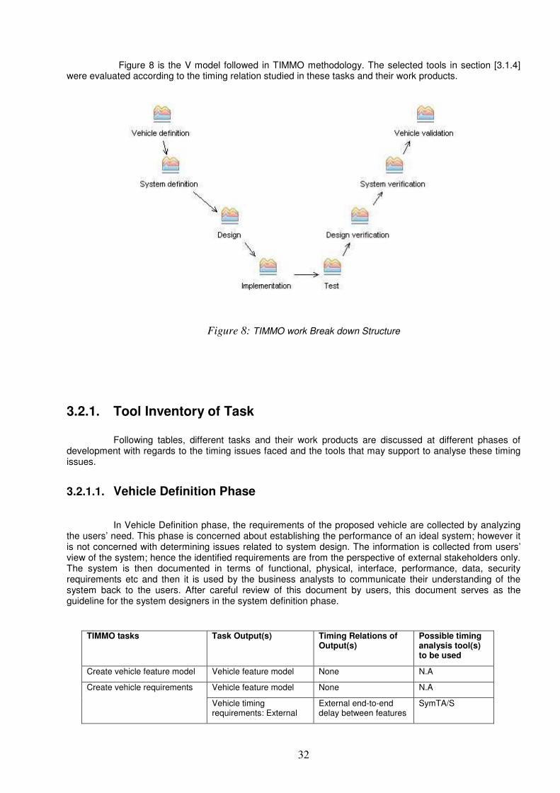
Figure 8 is the V model followed in TIMMO methodology. The selected tools in section [3.1.4] were evaluated according to the timing relation studied in these tasks and their work products.

Figure 8: TIMMO work Break down Structure

3.2.1. Tool Inventory of Task

Following tables, different tasks and their work products are discussed at different phases of

development with regards to the timing issues faced and the tools that may support to analyse these timing issues.

3.2.1.1. Vehicle Definition Phase

In Vehicle Definition phase, the requirements of the proposed vehicle are collected by analyzing the users’ need. This phase is concerned about establishing the performance of an ideal system; however it is not concerned with determining issues related to system design. The information is collected from users’ view of the system; hence the identified requirements are from the perspective of external stakeholders only. The system is then documented in terms of functional, physical, interface, performance, data, security requirements etc and then it is used by the business analysts to communicate their understanding of the system back to the users. After careful review of this document by users, this document serves as the guideline for the system designers in the system definition phase.

TIMMO tasks Task Output(s) Timing Relations of Output(s)

Possible timing analysis tool(s) to be used

Create vehicle feature model Vehicle feature model None N.A

Create vehicle requirements Vehicle feature model None N.A

Vehicle timing requirements: External

External end-to-end delay between features

SymTA/S

33

end-to-end delay

Vehicle timing requirements: Internal end-to-end delay

Internal end-to-end delay between features

SymTA/S, Cheddar

Vehicle timing requirements: Internal end-to-end delay

End-to-end delay SymTA/S

Vehicle timing requirements: Synchronization feature

Synchronisation between features

SymTA/S

Vehicle timing requirements: Synchronization feature

Synchronisation between features

SymTA/S

Validate timing requirements Timing requirement validation report

Validated timing requirements

BoundT, aiT, Cheddar, SymTA/S, MAST

Table 2: Tool Inventory in Vehicle Definition Phase

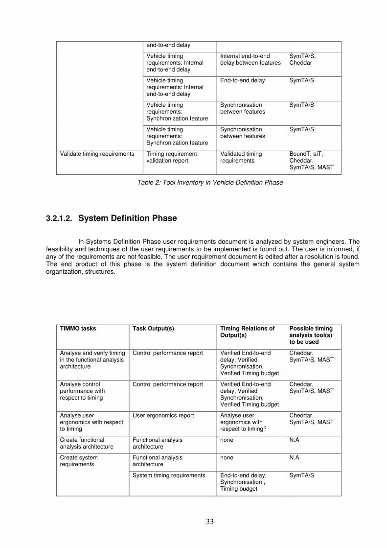
3.2.1.2. System Definition Phase

In Systems Definition Phase user requirements document is analyzed by system engineers. The feasibility and techniques of the user requirements to be implemented is found out. The user is informed, if any of the requirements are not feasible. The user requirement document is edited after a resolution is found. The end product of this phase is the system definition document which contains the general system organization, structures.

TIMMO tasks Task Output(s) Timing Relations of Output(s)

Possible timing analysis tool(s) to be used

Analyse and verify timing in the functional analysis architecture

Control performance report Verified End-to-end delay, Verified Synchronisation, Verified Timing budget

Cheddar, SymTA/S, MAST

Analyse control performance with respect to timing

Control performance report Verified End-to-end delay, Verified Synchronisation, Verified Timing budget

Cheddar, SymTA/S, MAST

Analyse user ergonomics with respect to timing

User ergonomics report Analyse user ergonomics with respect to timing?

Cheddar, SymTA/S, MAST

Create functional analysis architecture

Functional analysis architecture

none N.A

Create system requirements

Functional analysis architecture

none N.A

System timing requirements End-to-end delay, Synchronisation , Timing budget

SymTA/S

34

Table 3: Tool Inventory in System Definition Phase

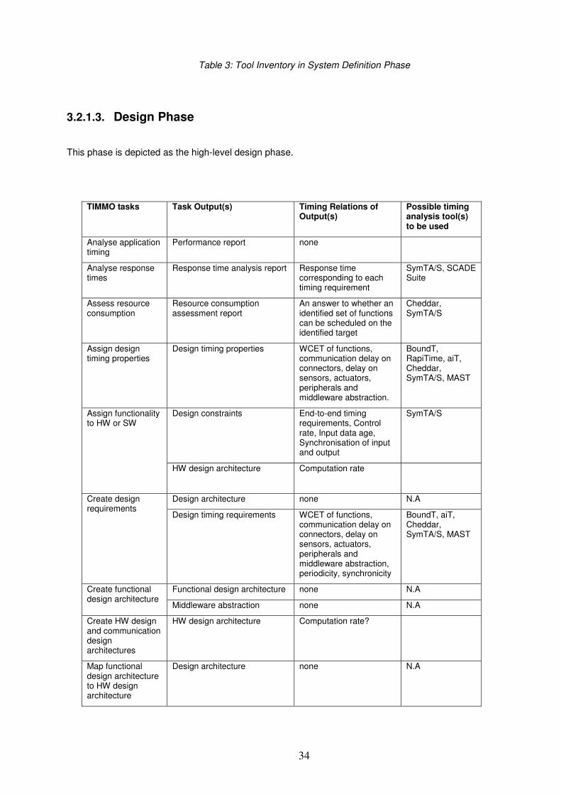
3.2.1.3. Design Phase

This phase is depicted as the high-level design phase.

TIMMO tasks Task Output(s) Timing Relations of Output(s)

Possible timing analysis tool(s) to be used

Analyse application timing

Performance report none

Analyse response times

Response time analysis report Response time corresponding to each timing requirement

SymTA/S, SCADE Suite

Assess resource consumption

Resource consumption assessment report

An answer to whether an identified set of functions can be scheduled on the identified target

Cheddar, SymTA/S

Assign design timing properties

Design timing properties WCET of functions, communication delay on connectors, delay on sensors, actuators, peripherals and middleware abstraction.

BoundT, RapiTime, aiT, Cheddar, SymTA/S, MAST

Assign functionality to HW or SW

Design constraints End-to-end timing requirements, Control rate, Input data age, Synchronisation of input and output

SymTA/S

HW design architecture Computation rate

Create design requirements

Design architecture none N.A

Design timing requirements WCET of functions, communication delay on connectors, delay on sensors, actuators, peripherals and middleware abstraction, periodicity, synchronicity

BoundT, aiT, Cheddar, SymTA/S, MAST

Create functional design architecture

Functional design architecture none N.A

Middleware abstraction none N.A

Create HW design and communication design architectures

HW design architecture Computation rate?

Map functional design architecture to HW design architecture

Design architecture none N.A

35

Design timing requirements WCET of functions, communication delay on connectors, delay on sensors, actuators, peripherals and middleware abstraction, periodicity, synchronicity

BoundT, aiT, Cheddar, SymTA/S, MAST

Table 4: Tool Inventory in Design Phase

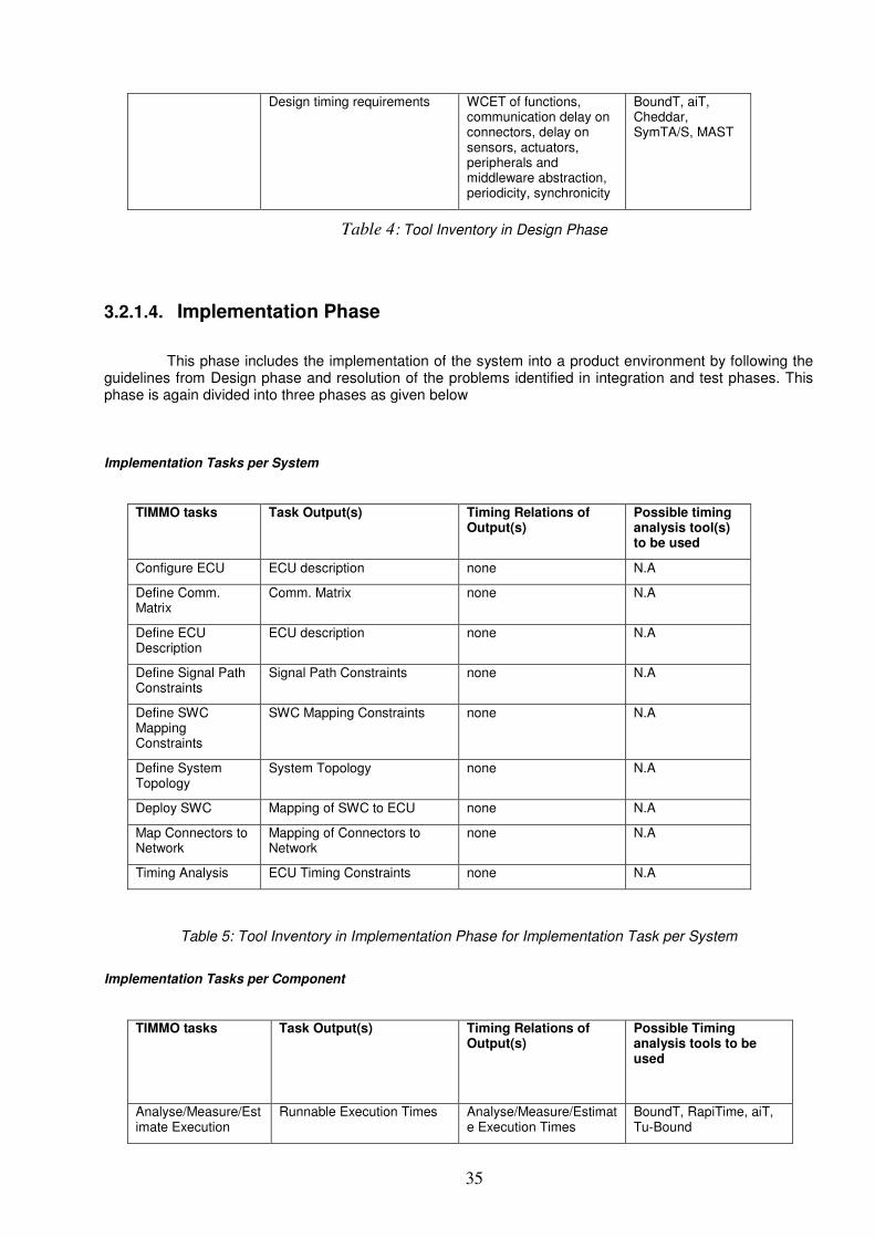
3.2.1.4. Implementation Phase

This phase includes the implementation of the system into a product environment by following the guidelines from Design phase and resolution of the problems identified in integration and test phases. This phase is again divided into three phases as given below

Implementation Tasks per System

TIMMO tasks Task Output(s) Timing Relations of Output(s)

Possible timing analysis tool(s) to be used

Configure ECU ECU description none N.A

Define Comm. Matrix

Comm. Matrix none N.A

Define ECU Description

ECU description none N.A

Define Signal Path Constraints

Signal Path Constraints none N.A

Define SWC Mapping Constraints

SWC Mapping Constraints none N.A

Define System Topology

System Topology none N.A

Deploy SWC Mapping of SWC to ECU none N.A

Map Connectors to Network

Mapping of Connectors to Network

none N.A

Timing Analysis ECU Timing Constraints none N.A

Table 5: Tool Inventory in Implementation Phase for Implementation Task per System

Implementation Tasks per Component

TIMMO tasks Task Output(s) Timing Relations of Output(s)

Possible Timing analysis tools to be used

Analyse/Measure/Estimate Execution

Runnable Execution Times Analyse/Measure/Estimate Execution Times

BoundT, RapiTime, aiT, Tu-Bound

36

Times

Define internal SWC behaviour and Runnables

Internal Behaviour and Runnables

none N.A

Implement SWC and Runnables

SWC and Runnable Implementation

none N.A

Create vehicle feature model

Vehicle feature model None N.A

Validate timing requirements

Timing requirement validation report

Validated timing requirements

Cheddar, SymTA/S, MAST

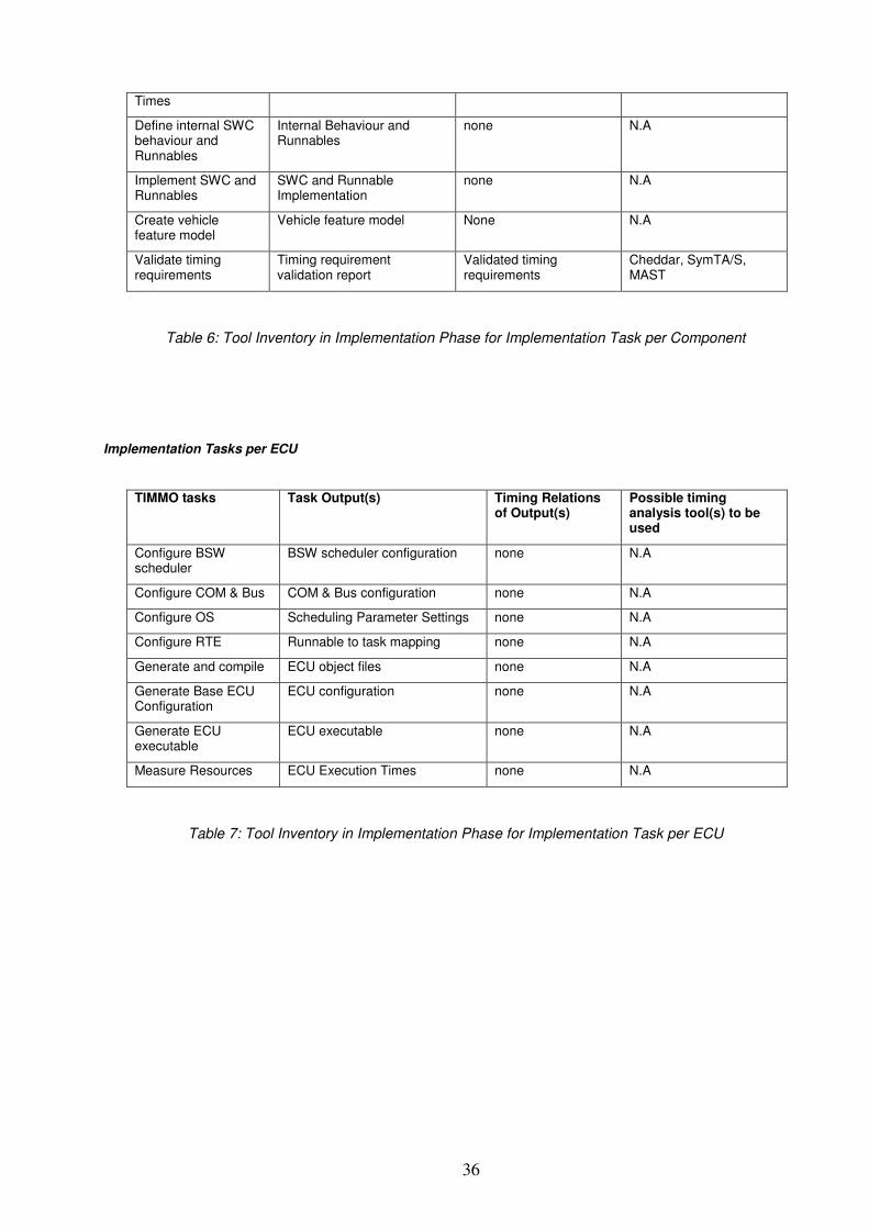
Table 6: Tool Inventory in Implementation Phase for Implementation Task per Component

Implementation Tasks per ECU

TIMMO tasks Task Output(s) Timing Relations of Output(s)

Possible timing analysis tool(s) to be used

Configure BSW scheduler

BSW scheduler configuration none N.A

Configure COM & Bus COM & Bus configuration none N.A

Configure OS Scheduling Parameter Settings none N.A

Configure RTE Runnable to task mapping none N.A

Generate and compile ECU object files none N.A

Generate Base ECU Configuration

ECU configuration none N.A

Generate ECU executable

ECU executable none N.A

Measure Resources ECU Execution Times none N.A

Table 7: Tool Inventory in Implementation Phase for Implementation Task per ECU

37

4. INFORMATION FLOW ANALYSIS

In every embedded system development, there is always use of different tools for different phases of system development starting from the system requirement gathering to maintenance and verification phase. These tools posses different functionality and are used with different purpose. As there is always some kind of dependency between one phase to another, the information gathered from one phase need to be passed on to the next phase(s). An improper flow of such information may lead to loss of information which may introduce faults in the system. The same problem may arise while using different tools. Therefore a careful study of information flow among such tools is required. This is also applicable to the timing information available in the tools.

In the following section, a brief description o f the tools used in TIMMO is given along with the information flow analysis of some of the tools is given.

4.1. Tools Used in TIMMO The development of the validators described in section mainly included tools for system design, simulation, timing analysis etc. These tools are Volcano VSA (Vehicle System Architecture) from Mentor Graphics, Vector tools (DaVinci System Architecture 2.3, DaVinci Network Designer 2.1 and DaVinci Developer 2.3) from Vectors, SymTA/S from Symtavision Gmbh, Eclipse with EPF plugin.

4.1.1. Volcano VSA:

VSA is a system architecture tool that facilities the design of embedded software system with AUTOSAR feature with support for FlexRay, CAN, and LIN network design. The tool uses a model-driven design process. It can be used to design, explore, and compare electronic and software architectures. VSA is based on the open-source with Eclipse Integrated Development Environment.

Features:

• VSA supports Software design architecture by defining software components and compositions and Hardware design architecture by defining ECUs, networks, sensors and actuators.

• It is a tool with AUTOSAR compliance and supports the AUTOSAR metamodel.

• Its scripting language support provides implementation of consistency checks or custom operations, which helps to ensure consistency of design data, both at the component and system level.

VSA provided the TIMMO editor that supported system design with the TIMMO Methodology. VSA could provide the following templates for this system design. Timingconstrains were defined and a connection with higher abstraction level of EAST_ADL2 and AUTOSAR. VSA provides a customized editor

to define an automotive system in terms of TIMMO Methodology and TADL. As shown in Figure 9, an ABS

system has been defined in TIMMO Editor provided by VSA with different parameters. AUTOSAR and EAST-ADL components of the system can be defined under the respective sections shown in this figure along with the timing constraints [47] in the section TimingConstraints. In Hardware design architecture information related to hardware used for the system is defined and so on.

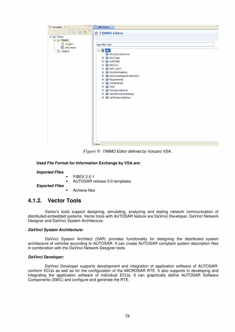
38

Figure 9: TIMMO Editor defined by Volcano VSA.

Used File Format for Information Exchange by VSA are: Imported Files

� FIBEX 2.0.1 � AUTOSAR release 3.0 templates

Exported Files � Achieve files

4.1.2. Vector Tools Vector's tools support designing, simulating, analyzing and testing network communication of distributed embedded systems. Vector tools with AUTOSAR feature are DaVinci Developer, DaVinci Network Designer and DaVinci System Architecture. DaVinci System Architecture: DaVinci System Architect (SAR) provides functionality for designing the distributed system architecture of vehicles according to AUTOSAR. It can create AUTOSAR compliant system description files in combination with the DaVinci Network Designer tools. DaVinci Developer: DaVinci Developer supports development and integration of application software of AUTOSAR-conform ECUs as well as for the configuration of the MICROSAR RTE. It also supports in developing and integrating the application software of individual ECUs. It can graphically define AUTOSAR Software Components (SWC) and configure and generate the RTE.

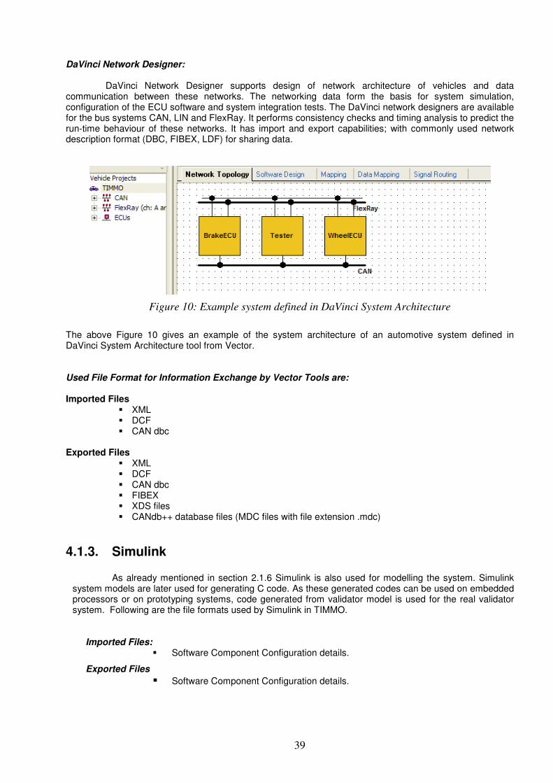
39

DaVinci Network Designer: DaVinci Network Designer supports design of network architecture of vehicles and data communication between these networks. The networking data form the basis for system simulation, configuration of the ECU software and system integration tests. The DaVinci network designers are available for the bus systems CAN, LIN and FlexRay. It performs consistency checks and timing analysis to predict the run-time behaviour of these networks. It has import and export capabilities; with commonly used network description format (DBC, FIBEX, LDF) for sharing data.

Figure 10: Example system defined in DaVinci System Architecture

The above Figure 10 gives an example of the system architecture of an automotive system defined in DaVinci System Architecture tool from Vector. Used File Format for Information Exchange by Vector Tools are: Imported Files

� XML � DCF � CAN dbc

Exported Files � XML � DCF � CAN dbc � FIBEX � XDS files � CANdb++ database files (MDC files with file extension .mdc)

4.1.3. Simulink

As already mentioned in section 2.1.6 Simulink is also used for modelling the system. Simulink system models are later used for generating C code. As these generated codes can be used on embedded processors or on prototyping systems, code generated from validator model is used for the real validator system. Following are the file formats used by Simulink in TIMMO.

Imported Files: � Software Component Configuration details.

Exported Files

� Software Component Configuration details.

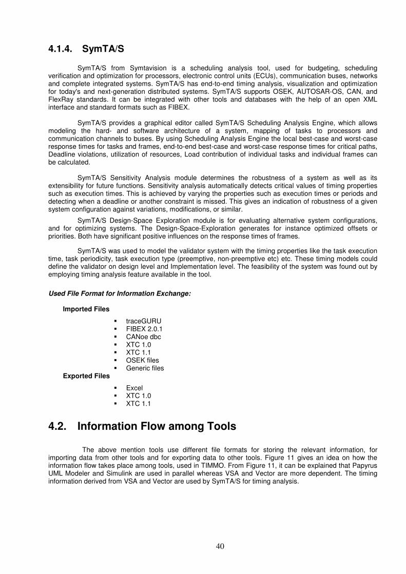
40

4.1.4. SymTA/S

SymTA/S from Symtavision is a scheduling analysis tool, used for budgeting, scheduling verification and optimization for processors, electronic control units (ECUs), communication buses, networks and complete integrated systems. SymTA/S has end-to-end timing analysis, visualization and optimization for today's and next-generation distributed systems. SymTA/S supports OSEK, AUTOSAR-OS, CAN, and FlexRay standards. It can be integrated with other tools and databases with the help of an open XML interface and standard formats such as FIBEX.

SymTA/S provides a graphical editor called SymTA/S Scheduling Analysis Engine, which allows modeling the hard- and software architecture of a system, mapping of tasks to processors and communication channels to buses. By using Scheduling Analysis Engine the local best-case and worst-case response times for tasks and frames, end-to-end best-case and worst-case response times for critical paths, Deadline violations, utilization of resources, Load contribution of individual tasks and individual frames can be calculated.

SymTA/S Sensitivity Analysis module determines the robustness of a system as well as its extensibility for future functions. Sensitivity analysis automatically detects critical values of timing properties such as execution times. This is achieved by varying the properties such as execution times or periods and detecting when a deadline or another constraint is missed. This gives an indication of robustness of a given system configuration against variations, modifications, or similar.

SymTA/S Design-Space Exploration module is for evaluating alternative system configurations, and for optimizing systems. The Design-Space-Exploration generates for instance optimized offsets or priorities. Both have significant positive influences on the response times of frames.

SymTA/S was used to model the validator system with the timing properties like the task execution time, task periodicity, task execution type (preemptive, non-preemptive etc) etc. These timing models could define the validator on design level and Implementation level. The feasibility of the system was found out by employing timing analysis feature available in the tool.

Used File Format for Information Exchange:

Imported Files

� traceGURU � FIBEX 2.0.1 � CANoe dbc � XTC 1.0 � XTC 1.1 � OSEK files � Generic files

Exported Files

� Excel � XTC 1.0 � XTC 1.1

4.2. Information Flow among Tools

The above mention tools use different file formats for storing the relevant information, for importing data from other tools and for exporting data to other tools. Figure 11 gives an idea on how the information flow takes place among tools, used in TIMMO. From Figure 11, it can be explained that Papyrus UML Modeler and Simulink are used in parallel whereas VSA and Vector are more dependent. The timing information derived from VSA and Vector are used by SymTA/S for timing analysis.

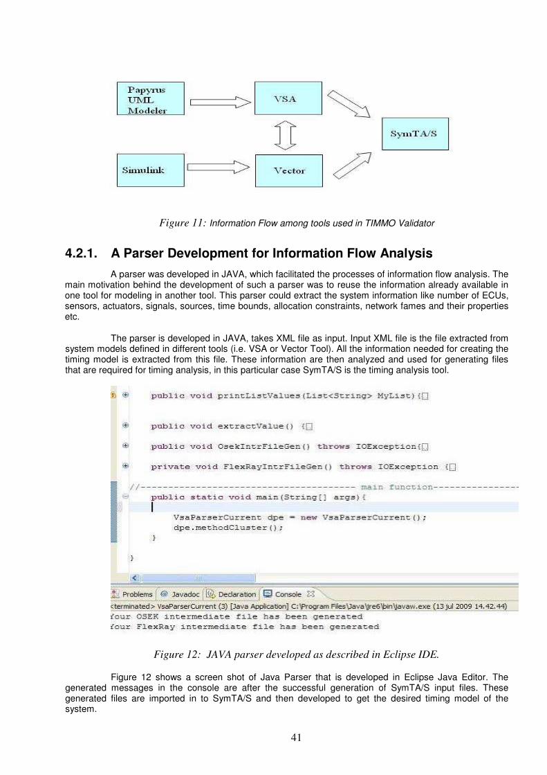
41

Figure 11: Information Flow among tools used in TIMMO Validator

4.2.1. A Parser Development for Information Flow Analysis

A parser was developed in JAVA, which facilitated the processes of information flow analysis. The main motivation behind the development of such a parser was to reuse the information already available in one tool for modeling in another tool. This parser could extract the system information like number of ECUs, sensors, actuators, signals, sources, time bounds, allocation constraints, network fames and their properties etc.

The parser is developed in JAVA, takes XML file as input. Input XML file is the file extracted from system models defined in different tools (i.e. VSA or Vector Tool). All the information needed for creating the timing model is extracted from this file. These information are then analyzed and used for generating files that are required for timing analysis, in this particular case SymTA/S is the timing analysis tool.

Figure 12: JAVA parser developed as described in Eclipse IDE.

Figure 12 shows a screen shot of Java Parser that is developed in Eclipse Java Editor. The generated messages in the console are after the successful generation of SymTA/S input files. These generated files are imported in to SymTA/S and then developed to get the desired timing model of the system.

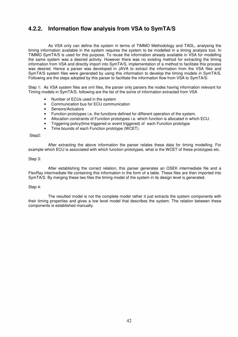
42

4.2.2. Information flow analysis from VSA to SymTA/S

As VSA only can define the system in terms of TIMMO Methodology and TADL, analysing the timing information available in the system requires the system to be modelled in a timing analysis tool. In TIMMO SymTA/S is used for this purpose. To reuse the information already available in VSA for modelling the same system was a desired activity. However there was no existing method for extracting the timing information from VSA and directly import into SymTA/S, implementation of a method to facilitate this process was desired. Hence a parser was developed in JAVA to extract the information from the VSA files and SymTA/S system files were generated by using this information to develop the timing models in SymTA/S. Following are the steps adopted by this parser to facilitate the information flow from VSA to SymTA/S:

Step 1: As VSA system files are xml files, the parser only parsers the nodes having information relevant for Timing models in SymTA/S. following are the list of the some of information extracted from VSA

• Number of ECUs used in the system

• Communication bus for ECU communication

• Sensors/Actuators

• Function prototypes i.e. the functions defined for different operation of the system.

• Allocation constraints of Function prototypes i.e. which function is allocated in which ECU.

• Triggering policy(time triggered or event triggered) of each Function prototype

• Time bounds of each Function prototype (WCET).

Step2:

After extracting the above information the parser relates these data for timing modelling. For example which ECU is associated with which function prototypes, what is the WCET of these prototypes etc.

Step 3:

After establishing the correct relation, this parser generates an OSEK intermediate file and a FlexRay intermediate file containing this information in the form of a table. These files are then imported into SymTA/S. By merging these two files the timing model of the system in its design level is generated.

Step 4:

The resulted model is not the complete model rather it just extracts the system components with their timing properties and gives a low level model that describes the system. The relation between these components is established manually.

43

Resulted Model:

Figure 13: Resulted model from the parser JAVA program

Figure 13 shows the resulted SymTA/S model after successfully analysing the timing information flow from VSA to SymTA/S, by following the above steps. The Heuristic developed in Chapter 6 has been used in the parser for generating this model.

4.2.3. Information flow analysis from Vector Tools to SymTA/S

Similar to the case in previous section there is also no integration between Vector tools and SymTA/S. Where a system can be defined in terms of AUTOSAR standards in Vector tools, defining the same system in SYMTA/S for timing analysis requires modeling the system again. Hence to reuse the information already available in Vector tools was also desired. In order to realise that a similar process to facilitate the information flow analysis between Vector tools and SymTA/S a similar parser was developed and some of the files developed were analysed in the similar fashion as depicted in section 4.2.2 above.

Following are the steps adopted by this parser to facilitate the information flow from Vector tools to SymTA/S:

Step 1: Different file formats are used by Vector tools. The systems defined by Vector Tools were extracted as xml files, the parser only parses the nodes having information relevant for Timing models in SymTA/S. following are the list of the some of information extracted from VSA

• No of ECUs used in the system

• Communication bus for ECU communication

• Runnables for each ECU

• Allocation constraints of the runnables

44

Step2:

After extracting the above informations the parser relates these data for timing modelling. For example which ECU is associated with which function prototypes, what is the WCET of these prototypes etc.

Step 3: After establishing the correct relation, this parser generates an OSEK intermediate file and a FlexRay intermediate file containing these informations in the form of a table. These files are then imported into SymTA/S. By merging these two files the timing model of the system in its design level is generated.

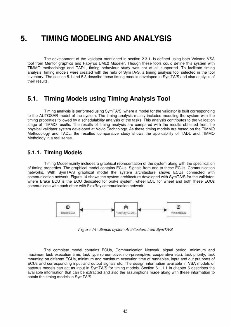
45

5. TIMING MODELING AND ANALYSIS

The development of the validator mentioned in section 2.3.1, is defined using both Volcano VSA tool from Mentor graphics and Papyrus UML2 Modeler. Though these tools could define this system with TIMMO methodology and TADL, timing behaviour study was not at all supported. To facilitate timing analysis, timing models were created with the help of SymTA/S, a timing analysis tool selected in the tool inventory. The section 5.1 and 5.3 describe these timing models developed in SymTA/S and also analysis of their results.

5.1. Timing Models using Timing Analysis Tool Timing analysis is performed using SymTA/S, where a model for the validator is built corresponding to the AUTOSAR model of the system. The timing analysis mainly includes modeling the system with the timing properties followed by a schedulability analysis of the tasks. This analysis contributes to the validation stage of TIMMO results. The results of timing analysis are compared with the results obtained from the physical validator system developed at Vovlo Technology. As these timing models are based on the TIMMO Methodology and TADL, the resulted comparative study shows the applicability of TADL and TIMMO Metholody in a real sense.

5.1.1. Timing Models Timing Model mainly includes a graphical representation of the system along with the specification of timing properties. The graphical model contains ECUs, Signals from and to these ECUs, Communication networks, With SymTA/S graphical model the system architecture shows ECUs connected with communication network. Figure 14 shows the system architecture developed with SymTA/S for the validator, where Brake ECU is the ECU dedicated for brake system, wheel ECU for wheel and both these ECUs communicate with each other with FlexRay communication network.

Figure 14: Simple system Architecture from SymTA/S

The complete model contains ECUs, Communication Network, signal period, minimum and maximum task execution time, task type (preemptive, non-preemptive, cooperative etc.), task priority, task mounting on different ECUs, minimum and maximum execution time of runnables, input and out put ports of ECUs and corresponding input and output signals etc. The design information available in VSA models or papyrus models can act as input in SymTA/S for timing models. Section 6.1.1.1 in chapter 6 describes the available information that can be extracted and also the assumptions made along with these information to obtain the timing models in SymTA/S.

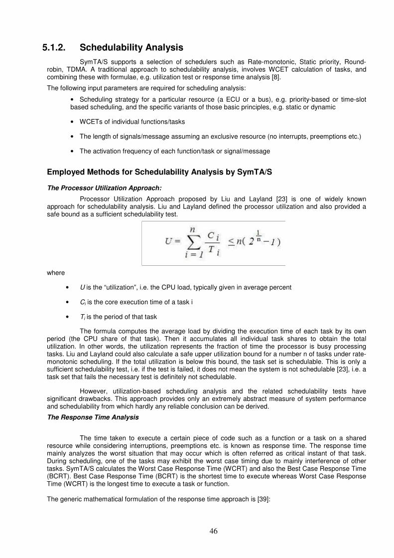
46

5.1.2. Schedulability Analysis

SymTA/S supports a selection of schedulers such as Rate-monotonic, Static priority, Round-robin, TDMA. A traditional approach to schedulability analysis, involves WCET calculation of tasks, and combining these with formulae, e.g. utilization test or response time analysis [8].

The following input parameters are required for scheduling analysis:

• Scheduling strategy for a particular resource (a ECU or a bus), e.g. priority-based or time-slot based scheduling, and the specific variants of those basic principles, e.g. static or dynamic

• WCETs of individual functions/tasks

• The length of signals/message assuming an exclusive resource (no interrupts, preemptions etc.)

• The activation frequency of each function/task or signal/message

Employed Methods for Schedulability Analysis by SymTA/S The Processor Utilization Approach:

Processor Utilization Approach proposed by Liu and Layland [23] is one of widely known approach for schedulability analysis. Liu and Layland defined the processor utilization and also provided a safe bound as a sufficient schedulability test.

where

• U is the “utilization”, i.e. the CPU load, typically given in average percent

• Ci is the core execution time of a task i

• Ti is the period of that task

The formula computes the average load by dividing the execution time of each task by its own period (the CPU share of that task). Then it accumulates all individual task shares to obtain the total utilization. In other words, the utilization represents the fraction of time the processor is busy processing tasks. Liu and Layland could also calculate a safe upper utilization bound for a number n of tasks under rate-monotonic scheduling. If the total utilization is below this bound, the task set is schedulable. This is only a sufficient schedulability test, i.e. if the test is failed, it does not mean the system is not schedulable [23], i.e. a task set that fails the necessary test is definitely not schedulable.

However, utilization-based scheduling analysis and the related schedulability tests have significant drawbacks. This approach provides only an extremely abstract measure of system performance and schedulability from which hardly any reliable conclusion can be derived.

The Response Time Analysis

The time taken to execute a certain piece of code such as a function or a task on a shared resource while considering interruptions, preemptions etc. is known as response time. The response time mainly analyzes the worst situation that may occur which is often referred as critical instant of that task. During scheduling, one of the tasks may exhibit the worst case timing due to mainly interference of other tasks. SymTA/S calculates the Worst Case Response Time (WCRT) and also the Best Case Response Time (BCRT). Best Case Response Time (BCRT) is the shortest time to execute whereas Worst Case Response Time (WCRT) is the longest time to execute a task or function. The generic mathematical formulation of the response time approach is [39]:

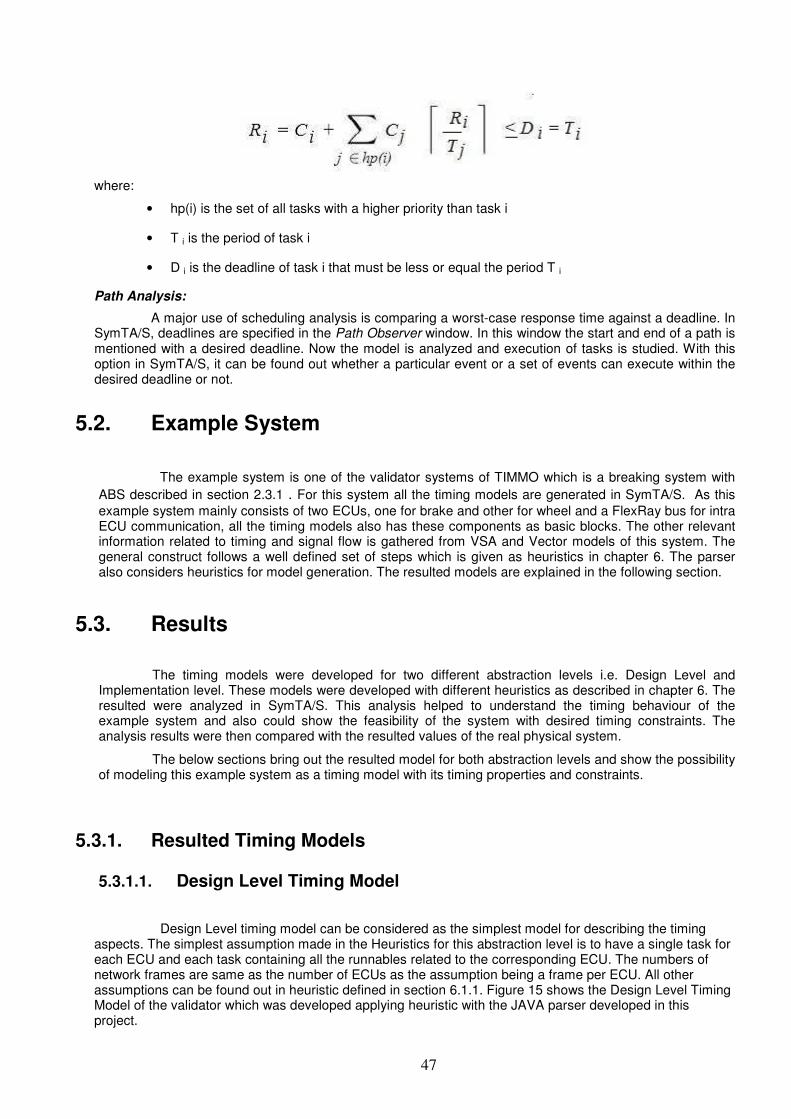
47

where:

• hp(i) is the set of all tasks with a higher priority than task i

• T i is the period of task i

• D i is the deadline of task i that must be less or equal the period T i

Path Analysis:

A major use of scheduling analysis is comparing a worst-case response time against a deadline. In SymTA/S, deadlines are specified in the Path Observer window. In this window the start and end of a path is mentioned with a desired deadline. Now the model is analyzed and execution of tasks is studied. With this option in SymTA/S, it can be found out whether a particular event or a set of events can execute within the desired deadline or not.

5.2. Example System

The example system is one of the validator systems of TIMMO which is a breaking system with

ABS described in section 2.3.1 . For this system all the timing models are generated in SymTA/S. As this

example system mainly consists of two ECUs, one for brake and other for wheel and a FlexRay bus for intra ECU communication, all the timing models also has these components as basic blocks. The other relevant information related to timing and signal flow is gathered from VSA and Vector models of this system. The general construct follows a well defined set of steps which is given as heuristics in chapter 6. The parser also considers heuristics for model generation. The resulted models are explained in the following section.

5.3. Results

The timing models were developed for two different abstraction levels i.e. Design Level and Implementation level. These models were developed with different heuristics as described in chapter 6. The resulted were analyzed in SymTA/S. This analysis helped to understand the timing behaviour of the example system and also could show the feasibility of the system with desired timing constraints. The analysis results were then compared with the resulted values of the real physical system.

The below sections bring out the resulted model for both abstraction levels and show the possibility of modeling this example system as a timing model with its timing properties and constraints.

5.3.1. Resulted Timing Models

5.3.1.1. Design Level Timing Model

Design Level timing model can be considered as the simplest model for describing the timing aspects. The simplest assumption made in the Heuristics for this abstraction level is to have a single task for each ECU and each task containing all the runnables related to the corresponding ECU. The numbers of network frames are same as the number of ECUs as the assumption being a frame per ECU. All other assumptions can be found out in heuristic defined in section 6.1.1. Figure 15 shows the Design Level Timing Model of the validator which was developed applying heuristic with the JAVA parser developed in this project.

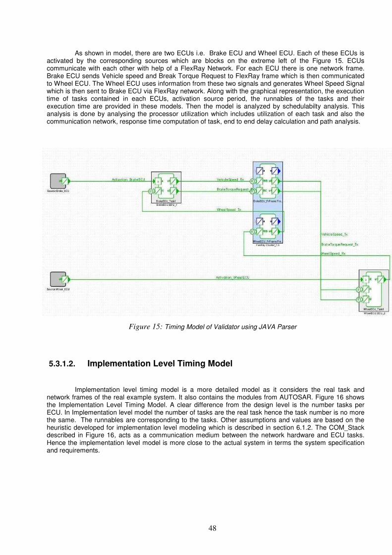
48

As shown in model, there are two ECUs i.e. Brake ECU and Wheel ECU. Each of these ECUs is activated by the corresponding sources which are blocks on the extreme left of the Figure 15. ECUs communicate with each other with help of a FlexRay Network. For each ECU there is one network frame. Brake ECU sends Vehicle speed and Break Torque Request to FlexRay frame which is then communicated to Wheel ECU. The Wheel ECU uses information from these two signals and generates Wheel Speed Signal which is then sent to Brake ECU via FlexRay network. Along with the graphical representation, the execution time of tasks contained in each ECUs, activation source period, the runnables of the tasks and their execution time are provided in these models. Then the model is analyzed by schedulabilty analysis. This analysis is done by analysing the processor utilization which includes utilization of each task and also the communication network, response time computation of task, end to end delay calculation and path analysis.

Figure 15: Timing Model of Validator using JAVA Parser

5.3.1.2. Implementation Level Timing Model

Implementation level timing model is a more detailed model as it considers the real task and network frames of the real example system. It also contains the modules from AUTOSAR. Figure 16 shows the Implementation Level Timing Model. A clear difference from the design level is the number tasks per ECU. In Implementation level model the number of tasks are the real task hence the task number is no more the same. The runnables are corresponding to the tasks. Other assumptions and values are based on the heuristic developed for implementation level modeling which is described in section 6.1.2. The COM_Stack described in Figure 16, acts as a communication medium between the network hardware and ECU tasks. Hence the implementation level model is more close to the actual system in terms the system specification and requirements.

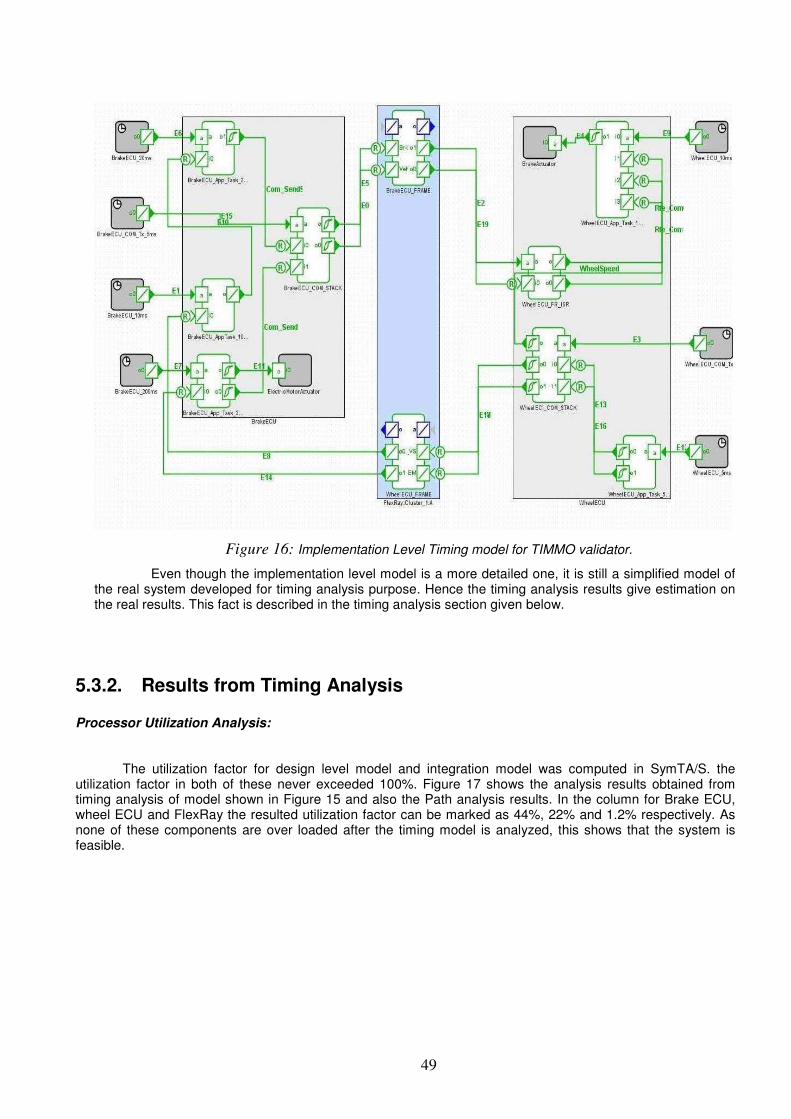
49

Figure 16: Implementation Level Timing model for TIMMO validator.

Even though the implementation level model is a more detailed one, it is still a simplified model of the real system developed for timing analysis purpose. Hence the timing analysis results give estimation on the real results. This fact is described in the timing analysis section given below.

5.3.2. Results from Timing Analysis

Processor Utilization Analysis:

The utilization factor for design level model and integration model was computed in SymTA/S. the utilization factor in both of these never exceeded 100%. Figure 17 shows the analysis results obtained from timing analysis of model shown in Figure 15 and also the Path analysis results. In the column for Brake ECU, wheel ECU and FlexRay the resulted utilization factor can be marked as 44%, 22% and 1.2% respectively. As none of these components are over loaded after the timing model is analyzed, this shows that the system is feasible.

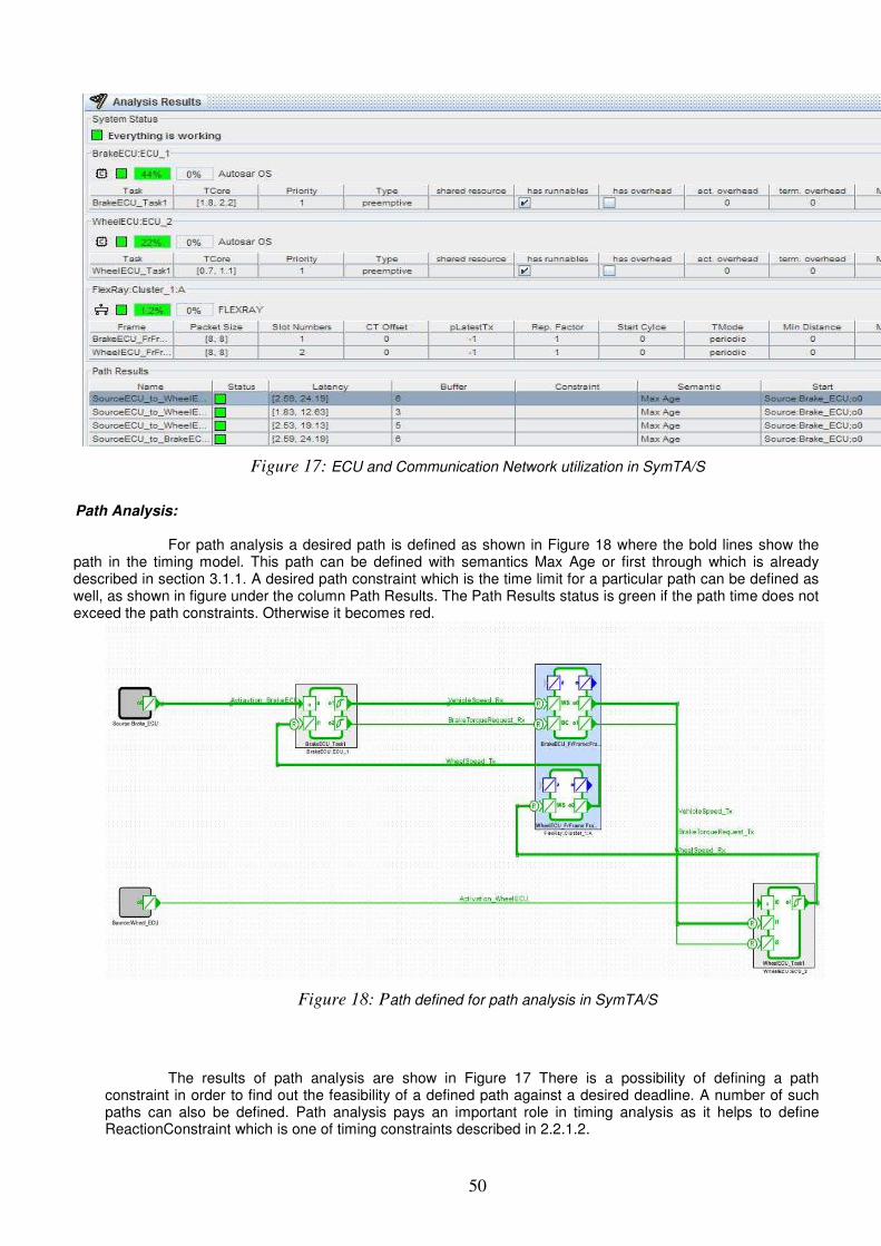
50

Figure 17: ECU and Communication Network utilization in SymTA/S

Path Analysis:

For path analysis a desired path is defined as shown in Figure 18 where the bold lines show the

path in the timing model. This path can be defined with semantics Max Age or first through which is already described in section 3.1.1. A desired path constraint which is the time limit for a particular path can be defined as well, as shown in figure under the column Path Results. The Path Results status is green if the path time does not exceed the path constraints. Otherwise it becomes red.

Figure 18: Path defined for path analysis in SymTA/S

The results of path analysis are show in Figure 17 There is a possibility of defining a path constraint in order to find out the feasibility of a defined path against a desired deadline. A number of such paths can also be defined. Path analysis pays an important role in timing analysis as it helps to define ReactionConstraint which is one of timing constraints described in 2.2.1.2.

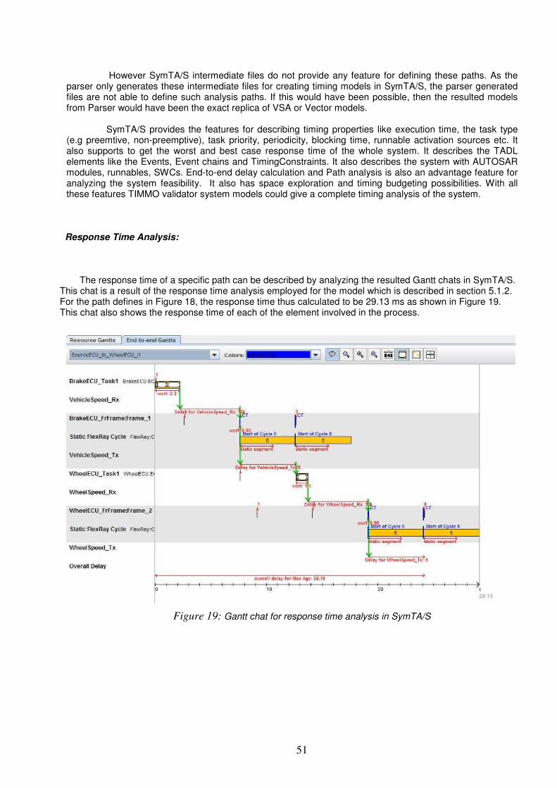
51

However SymTA/S intermediate files do not provide any feature for defining these paths. As the parser only generates these intermediate files for creating timing models in SymTA/S, the parser generated files are not able to define such analysis paths. If this would have been possible, then the resulted models from Parser would have been the exact replica of VSA or Vector models. SymTA/S provides the features for describing timing properties like execution time, the task type (e.g preemtive, non-preemptive), task priority, periodicity, blocking time, runnable activation sources etc. It also supports to get the worst and best case response time of the whole system. It describes the TADL elements like the Events, Event chains and TimingConstraints. It also describes the system with AUTOSAR modules, runnables, SWCs. End-to-end delay calculation and Path analysis is also an advantage feature for analyzing the system feasibility. It also has space exploration and timing budgeting possibilities. With all these features TIMMO validator system models could give a complete timing analysis of the system.

Response Time Analysis:

The response time of a specific path can be described by analyzing the resulted Gantt chats in SymTA/S. This chat is a result of the response time analysis employed for the model which is described in section 5.1.2. For the path defines in Figure 18, the response time thus calculated to be 29.13 ms as shown in Figure 19. This chat also shows the response time of each of the element involved in the process.

Figure 19: Gantt chat for response time analysis in SymTA/S

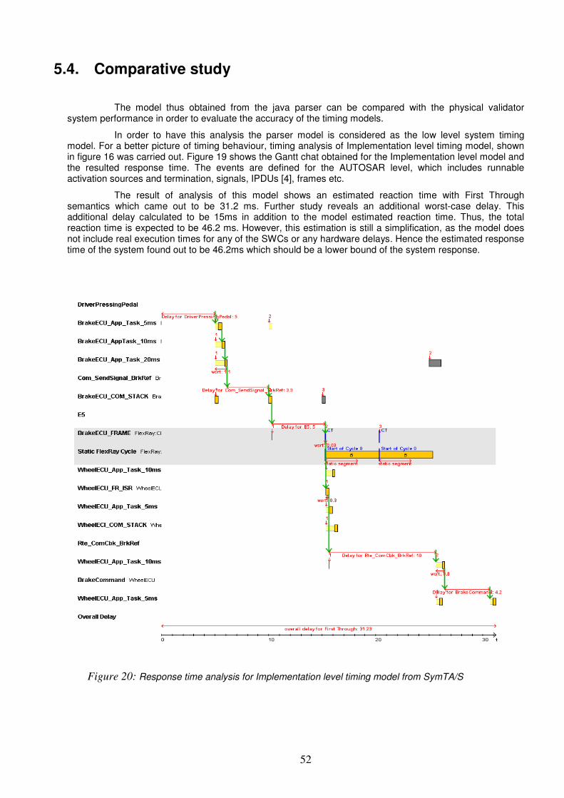
52

5.4. Comparative study

The model thus obtained from the java parser can be compared with the physical validator system performance in order to evaluate the accuracy of the timing models.

In order to have this analysis the parser model is considered as the low level system timing model. For a better picture of timing behaviour, timing analysis of Implementation level timing model, shown in figure 16 was carried out. Figure 19 shows the Gantt chat obtained for the Implementation level model and the resulted response time. The events are defined for the AUTOSAR level, which includes runnable activation sources and termination, signals, IPDUs [4], frames etc.

The result of analysis of this model shows an estimated reaction time with First Through semantics which came out to be 31.2 ms. Further study reveals an additional worst-case delay. This additional delay calculated to be 15ms in addition to the model estimated reaction time. Thus, the total reaction time is expected to be 46.2 ms. However, this estimation is still a simplification, as the model does not include real execution times for any of the SWCs or any hardware delays. Hence the estimated response time of the system found out to be 46.2ms which should be a lower bound of the system response.

Figure 20: Response time analysis for Implementation level timing model from SymTA/S

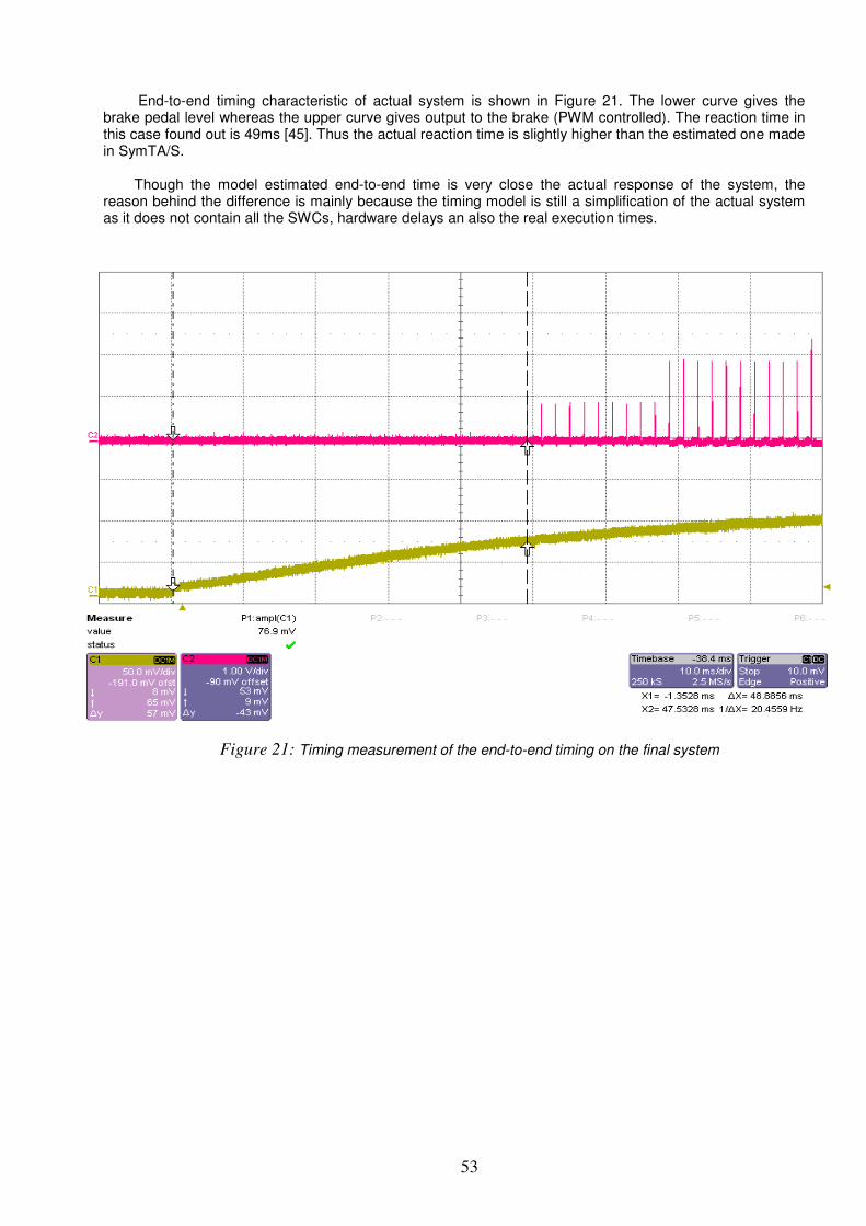
53

End-to-end timing characteristic of actual system is shown in Figure 21. The lower curve gives the brake pedal level whereas the upper curve gives output to the brake (PWM controlled). The reaction time in this case found out is 49ms [45]. Thus the actual reaction time is slightly higher than the estimated one made in SymTA/S.

Though the model estimated end-to-end time is very close the actual response of the system, the

reason behind the difference is mainly because the timing model is still a simplification of the actual system as it does not contain all the SWCs, hardware delays an also the real execution times.

Figure 21: Timing measurement of the end-to-end timing on the final system

54

55

6. HEURISTICS FOR TIMING MODELING

For developing a more accurate user model for timing analysis, following steps can be followed. These steps are given in more structured manner as Heuristics, which is described in the following sections. These heuristics are applied in both Design and Implementation level to get the timing models of the TIMMO validator. Before modeling a system some of the informations are derived from VSA system model which act as an input to these models. Along with these values some assumptions are also made to enhance these models. The parser developed for timing model, described in section followed these heuristics while generating the input files for SymTA/S.

6.1. Heuristics for Design Level & Implementation Level The available information for design level and implementation level are different. Hence the assumptions are taken differently. However the initial set up for both these abstraction levels does not differ greatly.

6.1.1. Heuristics for Design Level Modeling

6.1.1.1. Information & Assumption for Heuristics VSA model of an automotive system contains information that can be used in design level architecture.

Derived Values From VSA Model: Following is the list of values derived from VSA model of the validator system.

� The number of ECUs � Communication bus � Sensors/Actuators � Function prototypes � Allocation constraints of Function prototypes � Triggering policy(time triggered or event triggered) of each Function prototype � Time bounds of each Function prototype or WCET

Along with the above information some assumptions are taken for generating a timing model. Following are the list of assumptions made along with these values.

Assumptions:

� All ADLFunctions of a particular ECU are assumed to belong only to a single task. � Task type is taken as preemptive. � Execution time of each runnable is 0.1ms � Triggering policy(time triggered or event triggered) of each Function prototype

6.1.1.2. Heuristics for Initial Set Up:

Following parameters can be set for Design level Modelling of a system in SymTA/S Tasks:

• Each ECU contains one task.

• Tasks should be defined with properties like type of task, priority and runnables etc.

• For Design level modelling let task type for the tasks be preemptive

56

Runnables:

• As runnables are not essential in design level model, however for generating a user model in SymTA/S runnables are needed to be defined. Hence each ADLFunction is considered to be a single runnable. Thus the sum of WCET of all runnables, constrained to a particular ECU contributes to the total WCET of that ECU task.

• The number of runnables is the number of an ECU is the number of ADLFunctions related to that ECU.

Source:

• Single activation source should be connected to the activation port of each Task.

• Set source period to 5ms, if not specified by VSA Model

Ports:

• For each input and output operation, there should be a port other than activation port on each task.

Event Stream:

• Each signal from/to a port is represented by Event stream.

• Can be event triggered or registered. Core Execution Time (WCET):

• Each runnables should have a core execution time

• For simplicity start each runnables with execution time of 0.1ms if the execution time is unknown.

Task Type:

• Let the task type be Preemptive at the beginning for all the runnables.

• Tasks having a shared resource should be defined with shared object and should have task type as cooperative or preemptive.

• Those tasks that need to run uninterrupted should be defined as preemptive. Analysis Type:

• Let the task analysis type be Full Offset Analysis in order to analyse offsets with full accuracy.

• To analyse the system without overhead choose Offset Blind Analysis or choose Approximation Offset Analysis to analyse the offset between tasks that result from using synchronized sources.

Task priority:

• In case of a single task the task priority should be 1.

• For multiple task let each task is assigned in order of their execution.

• The higher priority task is assigned with higher digit in SymTA/S (i.e. a task with priority 5 has more priority over a task with priority 4).

Blocking time:

• Blocking time is 0 in the beginning.

• For a situation where a lower priority task needs to block a higher priority task for reasons other than cooperative or non-preemptive task blocking time should be mentioned.

Network:

57

• Communication between ECU to ECU should be through a Network. Network type can be CAN, LIN or FlexRay.

• Define one Network frame for each ECU.

• In case of FlexRay for each static frame there should be an activation port pair, which is left empty as per the specification of SymTA/S.

• In case of Dynamic frames the activation port should be connected to some activating signal. The activation signal could be any transmitted signal from any ECU or any independent signal.

Network Frame Ports:

• The no. of ports on each frame should be as per the input and output signals associated with it.

• Ports are always added in pairs.

• Frames can be synchronized with any of the source.

Frame Slot Number:

• Assign each frame with numbers starting from 1 to number of Frames defined. Com Bus:

Set

• Speed factor to 1

• Bus speed to 10,000 kHz

• Set scheduling to FLEXRAY and analysis to FlexRay analysis

6.1.1.3. Heuristics for System Analysis:

Heuristics for Utilization Factor Computation Step 1: Set Values

� Set core execution time (both minimum and maximum values)of each runnables to 0.1ms � Set Speed factor to 1 � Enable all runnables that needs to be analyzed

Step 2: Set Sources � Set all activation sources to 5ms

Step 3: Analyze � Analyze the system in SymTA/S.

Step 4: Result study

� The resulted values of utilization gives lower values of the utilization factor as the values taken for analysis are kept to minimum. In order to achieve a better result follow step 5 onwards.

� Init_Util = resulted utilization factor of each ECUs and communication bus Step 5: Result enhancement The following pseudo code gives steps for analysis where

resulted_Util_factor = Init_Util if (resulted_Util_factor > 50%)

runnables_min_exe_t = runnables_min_exe_t – 0.3 runnables_max_exe_t = runnables_max_exe_t – 0.3 Go to Step 3

Else if (resulted_Util_factor < 25%)

58

runnables_min_exe_t = runnables_min_exe_t + 0.5 runnables_max_exe_t = runnables_max_exe_t +0.5 Go to Step 3

Else

return resulted_Util_factor

Step 6: Repeat Step 5 until 25 %< resulted_Util_factor < 50%.

Step 7: Repeat Step 4-6 for all ECUs and communication networks. Heuristics for End-to-end Delay Calculation

Step 1: Set Values � Set initial value for execution time of each ECU to be 5ms. � Set task type to be non-preemptive. � Set a path for End-to-end delay computation with the start and the end point of the desired path. � Set semantics to max age for calculating the maximum path delay

Step 2: Define a path

� Define one or more paths for End to End Delay calculation � Set a desired start and end for the system � Set the path option with Max Age or First through, described in section

Step 3: Analyze

� Analyze the system in SymTA/S

Step 4: Result Study

� From Gantt chat check the response time for whole path � Response_t= first resulted response time from analysis

Step 5: Result Enhancement desired_Response_t = the desired response time for the path if ( Response_t > desired_Response_t)

Decrease source period Or

Increase runnables_min_exe_t, runnables_max_exe_t Go to Step 3

Else if (Response_t < desired_Response_t) Increase source period

Or Decrease runnables_min_exe_t, runnables_max_exe_t

Go to Step 3

Else

return Response_t Step 6: final response time = Response_t, from Step 5

59

6.1.2. Heuristics for Implementation Level Modeling

6.1.2.1. Information & Assumption for Heuristics

Derived Values From Vector Model: Following is the list of values derived from Vector model of the validator system.

� The number of ECUs � Communication bus � Sensors/Actuators � Signals and Signal Groups � Runnables � Runnables to task mapping � Communication ports � The “real” FlexRay parameters, i.e., the total number of frames, their slots etc.

Along with the above information some assumptions are taken for generating a timing model. Following are the list of assumptions made along with these values.

Assumption:

The known values before starting the Implementation level Model,

� Each ECU has a number of tasks which is equal to the number of ADLFunctions. The number of tasks are fewer or the same as the number of runnables, which in turn are same or fewer as the number of elementary ADLFunctions

� Each task has its own runnable(s). � input and output signals � Task priority and preemptiveness � COM and other BSW modules and their properties

6.1.2.2. Heuristic for Initial Set Up:

For Implementation level of system analysis initial set up will remain same as described in section 6.1.1.2 except for task, runnables and runnables.

• For each ECU, the number of task is the number of ADLFunctions define for ECU.

• The runnables are the runnables defined in the Software Developer model of Vector tools.

• Runnables are taken with their known execution time otherwise as per the assumption only if the values are not known.

• Source period are the period of the ADLFunction. In case the period is known, source may be chosen based on the deadline (e.g. 75% of desired deadline) .

6.1.2.3. Heuristic for System Analysis: Heuristics for Utilization Factor Computation

Step 1: Set Values

� Set core execution time (both minimum and maximum values)of each runnables to 0.1ms only if the core execution time is not known otherwise take the real-time bound defined

� Set Speed factor to 1 � Enable all runnables that needs to be analyzed

60

Step 2: Set Sources � Set all activation sources to 5ms if not specified otherwise take known values

Step 3: Analyze � Analyze the system in SymTA/S.

Step 4: Result study

� The resulted values of utilization gives lower values of the utilization factor as the values taken for analysis are kept to minimum. In order to achieve a better result follow step 5 onwards.

� Init_Util = resulted utilization factor of each ECUs and communication bus

Step 5: Result enhancement The following pseudo code gives steps for analysis where

resulted_Util_factor = Init_Util If (resulted_Util_factor > 100%) for each runnables {

runnables_min_exe_t = runnables_min_exe_t – 1ms runnables_max_exe_t = runnables_max_exe_t – 1ms } Go to Step 3 return resulted_Util_factor

Else if (resulted_Util_factor > 40% and resulted_Util_factor < 100%) Switch (resulted_Util_factor) Case 1: resulted_Util_factor < 60%

for each runnables {

runnables_min_exe_t = runnables_min_exe_t + runnables_min_exe_t * 0.2 runnables_max_exe_t = runnables_max_exe_t + runnables_min_exe_t * 0.2

} Go to Step 3

Case 2: 60 %< resulted_Util_factor < 80%

return resulted_Util_factor Case 3: 80% < resulted_Util_factor < 100%

for each runnables {

runnables_min_exe_t = runnables_min_exe_t - runnables_min_exe_t * 0.2 runnables_max_exe_t = runnables_max_exe_t - runnables_min_exe_t * 0.2 } Go to Step 3

Else if (resulted_Util_factor < 40%)

for each runnables { runnables_min_exe_t = runnables_min_exe_t + [1ms - 3ms] runnables_max_exe_t = runnables_max_exe_t + [1ms - 3ms]

} Go to Step 3 Else

61

return resulted_Util_factor

Step 6: repeat Step 5 until a more realistic values is not obtained Heuristics for End-to-end Delay Calculation

Step 1: Set Values � Set initial value for execution time of each ECU to be 5ms (if values are not known) � Set task type to be preemptive. � Set a path for End-to-end delay computation with the start and the end point of the desired path.

� Set semantics to Max age for calculating the maximum path delay with respect to the oldest data that can travel through the defined path or set semantics to first through to calculate maximum path delay with respect to the first signal that can traverse through the End-to-end signal path. � Declare constraint (i.e. deadline of a path) for the path if a desired deadline for particular path exists. If End-to-end delay of the path exceeds path constrains the analysis fails and the path is marked as red.

Step 2: Define a path

� Define one or more paths for End to End Delay calculation � Set a desired start and end for the system � Set the path option with Max Age or First through, described in section 3.1.1 for SymTA/S

Step 3: Analyze

� Analyze the system in SymTA/S � Got to Step 4

Step 4: Result Study � From gnatt chat check the response time for whole path � Response_t= first resulted response time from analysis � Go to step 5

Step 5: Result Enhancement desired_Response_t = the desired response time for the path if ( Response_t > desired_Response_t)

Decrease source period Or

Increase runnables_min_exe_t, runnables_max_exe_t Go to Step 3 return Response_t

Else if (Response_t < desired_Response_t) Increase source period

Or Decrease runnables_min_exe_t, runnables_max_exe_t

Go to Step 3

return Response_t

Else

return Response_t Step 6: final response time = Response_t, from Step 5

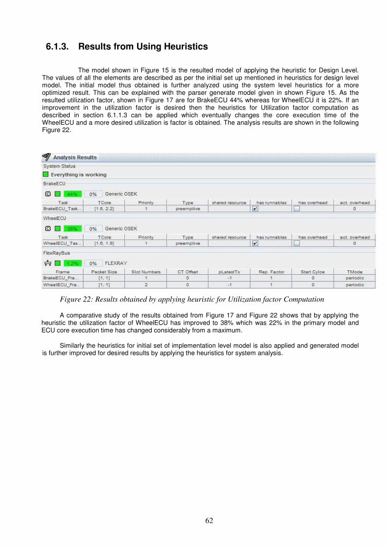
62

6.1.3. Results from Using Heuristics

The model shown in Figure 15 is the resulted model of applying the heuristic for Design Level. The values of all the elements are described as per the initial set up mentioned in heuristics for design level model. The initial model thus obtained is further analyzed using the system level heuristics for a more optimized result. This can be explained with the parser generate model given in shown Figure 15. As the resulted utilization factor, shown in Figure 17 are for BrakeECU 44% whereas for WheelECU it is 22%. If an improvement in the utilization factor is desired then the heuristics for Utilization factor computation as described in section 6.1.1.3 can be applied which eventually changes the core execution time of the WheelECU and a more desired utilization is factor is obtained. The analysis results are shown in the following Figure 22.

Figure 22: Results obtained by applying heuristic for Utilization factor Computation

A comparative study of the results obtained from Figure 17 and Figure 22 shows that by applying the heuristic the utilization factor of WheelECU has improved to 38% which was 22% in the primary model and ECU core execution time has changed considerably from a maximum.

Similarly the heuristics for initial set of implementation level model is also applied and generated model is further improved for desired results by applying the heuristics for system analysis.

63

7. ANALYSIS OF RESULTS

This section analyzes the results obtained from different activities carried out during this thesis work.

Tool Survey: The tool survey gave a list of timing analysis tools which could be used for automotive embedded

systems. A comprehensive study of their features, usability, automotive relevance and limitation was made, described in section 3.1.1. This list contains both the academic and commercial tools. This list is not only useful in TIMMO validation process but a useful handy list for any other automotive project, which might require a list of timing analysis tools. These tools further evaluated for a tool inventory.

Tool Inventory:

Tool selection with specification of TIMMO validator was carried out in this phase. This involved a

careful study of TIMMO validator requirements and also analysis of timing analysis tools. The selections of most suitable ones were made as per the validator requirement. This process could bring out a more clear understanding of advantages and limitations of these tools. These activities are explained in section 3.2.

Timing Models:

The timing models were developed using SymTA/S. These models describes in section 5.3.1

helped to realize the validator system with timing information and timing behaviour. Different analysis methods employed could hep to decide the feasibility of the system. These models also could give an idea on the response time of defined paths though being simplified models of the real one. A comparative study all reveals the correctness and accuracy of these results in comparison to the results obtained from physical system. The timing analysis of the validator system however demanded an accurate knowledge of timing information such as WCET, deadlines, task types (preemptive, non-preemptive etc), periodicity etc prior to modelling. This information may not be most likely present for every kind of automotive systems. However timing information gathered from experience of working with similar systems or an educated guess of the timing behaviour may still help to define these timing properties.

Heuristics:

The Heuristics, from chapter 6, was developed for timing modeling gives steps for generating these models and at same time guides to improve them further to match the desired results. These Heuristics were verified in different abstraction levels to find out its usability. The parser developed of study of information flow also follows these steps while modeling.

Timing Information Flow Analysis:

The information flow analysis (chapter 4) of different tools used for TIMMO validator showed the possibility of transferring the time related information from one tool to another to have different representation of a single system. Parser developed with a purpose of accelerating the information exchange could successfully extracted the necessary timing information from one tool and could generate input files for another tool based on these information. These helped to avoid the process of re-engineering work while switching from one tool to another.

64

8. CONCLUSION

The work carried out during this thesis work could define the Validator system with its timing

properties in SymTA/S, a tool which is one of the well evaluated tools from tool inventory and thus help to analyze the system in different abstraction levels. Though there can be many possible ways for timing analysis of TIMMO validator, however the use of selected tools is found out to be very useful. Timing analysis by using these tools reused the work and efforts already made for studying the timing properties and also lessened time and efforts employed for it.

Results obtained in this project show that TADL allows modelling of timing properties of

automotive embedded systems at all abstraction levels, defined by EAST-AD2 and can be used to model timing information for AUTOSAR-based systems. TADL can detect and analyze timing issues of an automotive system. The use of right tool-support can shorten the time required for development cycles. However, more work is needed to harmonize tools and tool concepts for modelling, timing annotation and timing analysis with a sound theoretical foundation of TADL. This can be achieved by enabling the use of TADL as an exchange format for this type of information, enabling exploitation of tools from different vendors, each having specific purposes and benefits. In the case of Volvo Validator, this is illustrated by the exchange of information across VSA and SymTA/S.

65

9. FUTURE WORK

Modeling the validator system with more than one or possibly all selected tools from tool

inventory is more desirable in future. The use of different tools for modeling will not only over come the draw backs of each other but will also provide a comparative study of the timing models. This will definitely improve the understanding of the timing properties and will open up the challenges and difficulties of modeling.

In current scenario the validator is only a single system, in this case an ABS system. As the behaviour of the system is greatly influenced in the presence of other systems, it is always useful to understand the timing behaviour of a combination of systems. Hence to understand the variation in the system behaviour a cluster of these systems should be considered and should be reflected in its timing models.

The heuristics should be defined for all abstraction level of vehicle modeling than just few of them. To achieve this, modeling requirement for each of these abstraction levels should be well understood and analyzed before hand.

Information flow analysis can be improved with the development of an intelligent tool that

automates the extraction of timing information and uses these informations for generating timing models.

The future endeavours will be on finding out the other possible ways, other than using timing analysis tools for analysing the timing behaviour of automotive embedded systems. This may involve study of different timing analysis methods focusing embedded systems and ways in which these methods are employed.

66

10. REFERENCES

[1] "AADL, an SAE Standard",http://www.aadl.info/aadl/currentsite/start/index.html,acessed on February 2009,

[2] "About", http://www.otawa.fr/, accessed on February 2009

[3] "ABOUT AUTOSAR", http://www.autosar.org/ index.Php? p=1&up=0&uup=0&uuup=0, accessed on 20th February 2009

[4] ACM Transactions on Embedded Computing Systems, The Worst-Case Execution Time Problem— Overview of Methods and Survey of Tools, Vol. V, No. N, Month 20YY, Pages 1–47.

[5] "aiT Worst-Case Execution Time Analyzers", http://www.absint.com/ait/, accessed on February 2009, Absint

[6] "A UML Profile for MARTE, Beta 1", http://www.omg.org/cgi-bin/doc?ptc/2007-08-04, accessed on June 2009

[7] "Bound-T", http://www.tidorum.fi/bound-t/, accessed on February 2009.

[8] A. Burns and A. Wellings, Real-Time Systems and Programming Languages, Addison Wesley Longmain, 2001

[9] F.Cassez, o.Roux, "From Time Petri Nets to Timed Automata", by Elsevier Science B. V., 2004

[10] "Chronos", http://www.comp.nus.edu.sg/~rpembed/chronos/, accessed on February 2009

[11] "Common Warehouse Metamodel (CWM) Specification",http://www.omg.org/docs/formal/03-03-02.pdf

[12] "EAST-ADL2 Language and Profile", http: //www.atesst.org /scripts /home/publigen/content/templates/ show.asp?P=125&L=EN&ITEMID=6,accessed on February 2009

[13] A. Gupta, V. Kahlon, and N. Sinha Symbolic Model Checking of Concurrent Programs using Partial Orders and On-the-fly Transactions. Computer Aided Verification (CAV), August 2006

[14] Jan Gustafsson. The WCET Tool Challenge 2006, 2nd International Symposium on Leveraging Applications of Formal Methods (SOLA'06), p 248-249, Paphos, Cyprus, November, 2007

[15] Xiao He (2007). "A metamodel for the notation of graphical modeling languages". In: Computer Software and Applications Conference, 2007. COMPSAC 2007 - Vol. 1. 31st Annual International, Volume 1, Issue, 24-27 July 2007, pp 219-224.

[16] "HEPTANE User Documentation (Version 1.0) ", http://www.irisa.fr/aces/work/heptane-demo/user/index. html, accessed on February 2009

[17] "Industry Links", http://www.svug.org/AboutUs/tabid/54/Default.aspx, accessed on February 2009.

[18] "Introduction to OMG's Unified Modeling Language™ (UML®)", http://www.omg.Org/gettingstarted/ what_is_uml.htm, accessed on February 2009.

[19] "Introduction",http://mast.unican.es/, accessed on February 2009.

[20] M. Joseph. P. Pandya,”Finding response times in a real-time system.” The Computer Journal. 29(5). Pages 390–395. 1986.

67

[21] J.P. Lehoczky, “Real-Time Queueing Theory,” Proceedings of the IEEE Real-Time Systems Symposium, pp. 186–195, 1996.

[22] J. Lehoczky. L. Sha. Y. Ding. The rate monotonic scheduling algorithm: Exact characterization and average case behaviour. In Proceedings Real-Time Systems Symposiom. IEEE Computer Society Press. Pages 166–171. 1989.

[23] C.L. Liu. J.W. Layland. Scheduling algorithms for multiprogramming in a hard real- time environment. Journal of the ACM. 20(1). pages 46–61. 1973.

[24] Matthew Hause Artisan Software Tools, Eagle Tower Suite 701, Cheltenham, Glos. UK,” The SysML Modelling Language, Fifth European Systems Engineering Conference”, 18-20 September 2006

[25] "OMG's MetaObject Facility", http://www.omg.org/mof/, accessed on June 2009

[26] "Overview", http://www.systemverilog.org/overview/overview.html, accessed on June 2009.

[27] J.C. Palencia. M. G. Harbour, Exploiting precedence relations in the schedulability analysis of distributed real-time systems, In Proceedings of the IEEE Real-Time Systems Symposium. Pages 328–399. 1999.

[28] "RAPID RMA: The Art of Modeling Real-Time Systems", http://www.tripac.com/html/prod-fact-rrm.html, accessed on February 2009.

[29] "RapiTime On Target Timing Analysis", http://www.rapitasystems.com/rapitime, accessed on February 2009, Rapita Systems Ltd.

[30] "RT-Druid", http://www.evidence.eu.com/content/view/28/51/, accessed on February 2009.

[31] "SCADE Suite", http://www.esterel-technologies.com/products/scade-suite/, accessed on February 2009, ESTEREL Technology.

[32] "Simulink - Simulation and Model-Based Design",http://www.mathworks.com/products/simulink/, accessed on June 2009, Mathworks.

[33] "Software & Systems Process Engineering Metamodel Specification, v2.0 (Beta 2)", http://www.omg.org/ spec/SPEM/2.0/Beta2/PDF, accessed on June 2009.

[34] "SymTA/S Overview", http://www.symtavision.com/products.html, accessed on February 2009.

[35] "SysML - Open Source Specification Project", http://www.sysml.org/, accessed on June 2009.

[36] "SWEET (SWEdish Execution Time tool) ", http://www.mrtc.mdh.se/projects/wcet/sweet.html, accessed on February 2009.

[37] "The Object Management Group (OMG)", http://www.omg.org/, accessed on June 2009.

[38] "The Timing Definition Language", http://se.ethz.ch/laser/2005/slides/pree/02a_TDL.pdf, accessed on July 2009

[39] "TIMMO - MASTERING IN-VEHICLE TIMING CONSTRAINTS", https://www.timmo.org/overview.htm, accessed on June 2009.

[40] "TuBound", http://costa.tuwien.ac.at/tubound.html, accessed on February 2009.

[41] TIMMO Partners, Conceptual Framework V1, Version 1.2, 28th November 2008.

[42] TIMMO Parnters, TIMMO Project, Deliverable D8, Validator Documentation, Version 0.6, 16.06.2009

[43] Ken Tindell, Real Time Systems and Fixed Priority Scheduling, Department of Computer Systems, Uppsala University, March 30, 1995.

68

[44] "User’sManual WCET-Analysis Framework based on WCETC", http://www.vmars.Tuwien.ac.at/ ~ raimund/calc_wcet/, accessed on

[45] "WCET Analysis at TU-Vienna", http://www.wcet.at/, accessed on February 2009.

[46] "What is Cheddar ? ", http://beru.univ-brest.fr/~singhoff/cheddar/, accessed on February 2009.

[47] Jia Xu, David Lorge Parnas, On Satisfying Timing Constraints in Hard-Real-Time Systems, Senor Member, IEEE, IEEE Transaction on Software Engineering, VOL. 19, NO. 1, January 1993.

69

11. GLOSSARY

AADL: Architecture Analysis & Design Language, developed by a Society of Automotive Engineers (SAE) ABS: Anti- Lock Braking System, an Automotive Embedded System AUTOSAR: AUTomotive Open System Architecture, open and standardized automotive software architecture BCET: Best Case Execution Time BCM: Body Control Module BCRT: Best Case Response Time BDD: Binary decision diagrams CAN: Controller Area Network, a vehicle bus standard designed to allow microcontrollers and devices to communicate with each other CFG: Control flow graphs CPU: Control Processing Unit CWM: Common Warehouse Metamodel DASPCP: Distributed Affected Set Priority Ceiling Protocol DBC: a file format used in CAN database of Vector Informatik Gmbh., is used to store information that describes CAN network DCF: DaVinci Configuration File. DM: Dead Line Monotonic DMA: Dead Line Monotonic Analysis DSL: Domain-specific language DSM: Domain-specific modeling ECM : Engine Control Module ECU: Electronic Control Unit EDF: Earliest-Deadline-First EPF: Eclipse Process Framework EPS: Electric power steering, an automotive embedded system. FAA: Functional Analysis Architecture FDA: Functional Design Architecture FIBEX: Field Bus Exchange Format, an xml file format adopted by the automotive industry for networks data/information exchange. FIFO: First In First Out FSM: Finite State Machine GNU: A computer operating system composed entirely of free software. GPL: General Public License, a free software license used for the GNU project HDL: Hardware Description Language used for formal description of digital logic and electronic circuits IPET: Implicit Path Enumeration Technique IR: Intermediate representation LDF: Layered Data Format, a file format LET: Logical Execution Time LIN: Local Interconnect Network, a vehicle bus standard or computer networking bus-system used within automotive network architectures. LLF: Least Laxity First, LTL: Linear temporal logic, a modal temporal logic with modalities referring to time. MARTE: Model-based Approach to Real-Time Embedded Systems development MOF: Meta Object Facility MOST: Media Oriented Systems Transport OEM: Original Equipment Manufacturer OMG: Object Management Group OMT: Object-modeling technique OOSE: Object-oriented software engineering OSEK: (Offene Systeme und deren Schnittstellen für die Elektronik in Kraftfahrzeugen); English: "Open Systems and their Interfaces for the Electronics in Motor Vehicles"), a standards body that has produced specifications for an embedded operating system, a communications stack, and a network management protocol for automotive embedded systems. PSL: Process Specification Language RM: Rate Monotonic

70

RMA: Rate Monotonic Analysis RTA: Response time schedulability analysis RTQT: Real-Time Queuing Theory SPF: Single Feasible Paths SPEM: Software Process Engineering Metamodel SPT: Schedulability, Performance and Time SSF: Space Systems Finland Ltd SWC: Software Component SysML: Systems Modeling Language TADL: Timing Augmented Descriptive Language TDL: Timing Definition Language TIMMO: Timing Model UML: Unified Modeling Language VHDL: Very High Speed Integrated Circuits VSA: Vehicle Systems Architect WCET: Worst Case Execution Time WCRT: Worst Case Response Time XTC: XML Timing cookie.

�