Today

• Path Planning– Intro

– Waypoints

– A* Path Planning

Path Finding

• Very common problem in games:– In FPS: How does the AI get from room to room?

– In RTS: User clicks on units, tells them to go somewhere. How do they get there? How do they avoid each other?

– Chase games, sports games, …

• Very expensive part of games– Lots of techniques that offer quality, robustness, speed trade-offs

Path Finding Problem

• Problem Statement (Academic): Given a start point, A, and a goal point, B, find a path from A to B that is clear– Generally want to minimize a cost: distance, travel time, …

• Travel time depends on terrain, for instance

– May be complicated by dynamic changes: paths being blocked or removed

– May be complicated by unknowns – don’t have complete information

• Problem Statement (Games): Find a reasonable path that gets the object from A to B– Reasonable may not be optimal – not shortest, for instance

– It may be OK to pass through things sometimes

– It may be OK to make mistakes and have to backtrack

Search or Optimization?

• Path planning (also called route-finding) can be phrased as a search problem:– Find a path to the goal B that minimizes Cost(path)– There are a wealth of ways to solve search problems, and we will look at

some of them

• Path planning is also an optimization problem:– Minimize Cost(path) subject to the constraint that path joins A and B

• State space is paths joining A and B, kind of messy

– There are a wealth of ways to solve optimization problems

• The difference is mainly one of terminology: different communities (AI vs. Optimization)– But, search is normally on a discrete state space

Brief Overview of Techniques

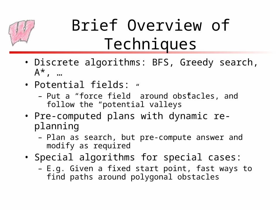
• Discrete algorithms: BFS, Greedy search, A*, …• Potential fields:

– Put a “force field” around obstacles, and follow the “potential valleys”

• Pre-computed plans with dynamic re-planning– Plan as search, but pre-compute answer and modify as required

• Special algorithms for special cases:– E.g. Given a fixed start point, fast ways to find paths around

polygonal obstacles

Graph-Based Algorithms

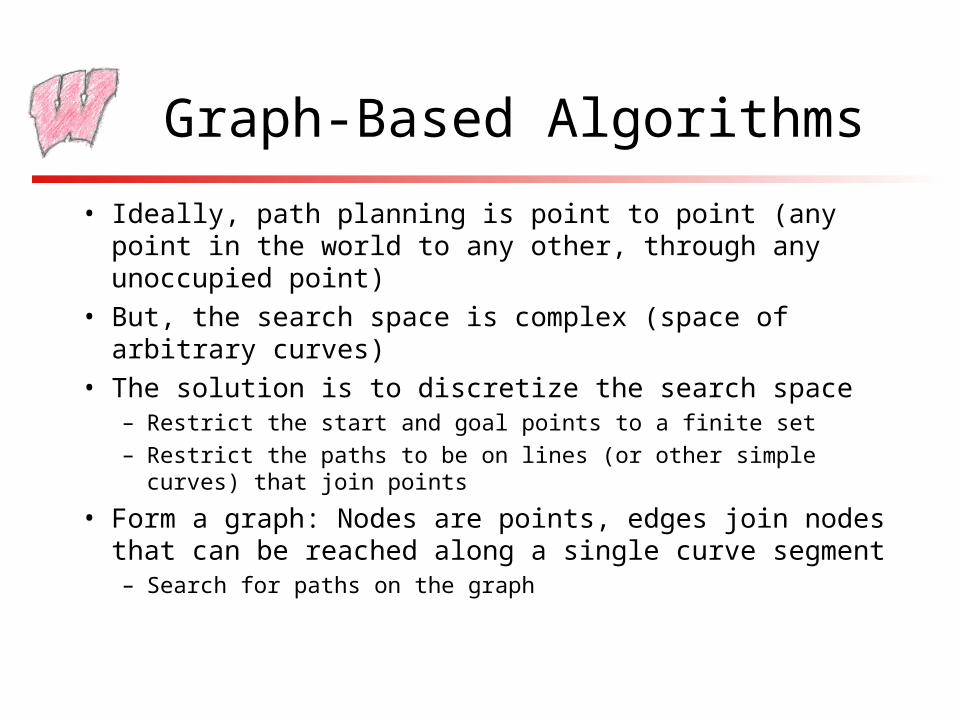
• Ideally, path planning is point to point (any point in the world to any other, through any unoccupied point)

• But, the search space is complex (space of arbitrary curves)

• The solution is to discretize the search space– Restrict the start and goal points to a finite set

– Restrict the paths to be on lines (or other simple curves) that join points

• Form a graph: Nodes are points, edges join nodes that can be reached along a single curve segment– Search for paths on the graph

Waypoints (and Questions)

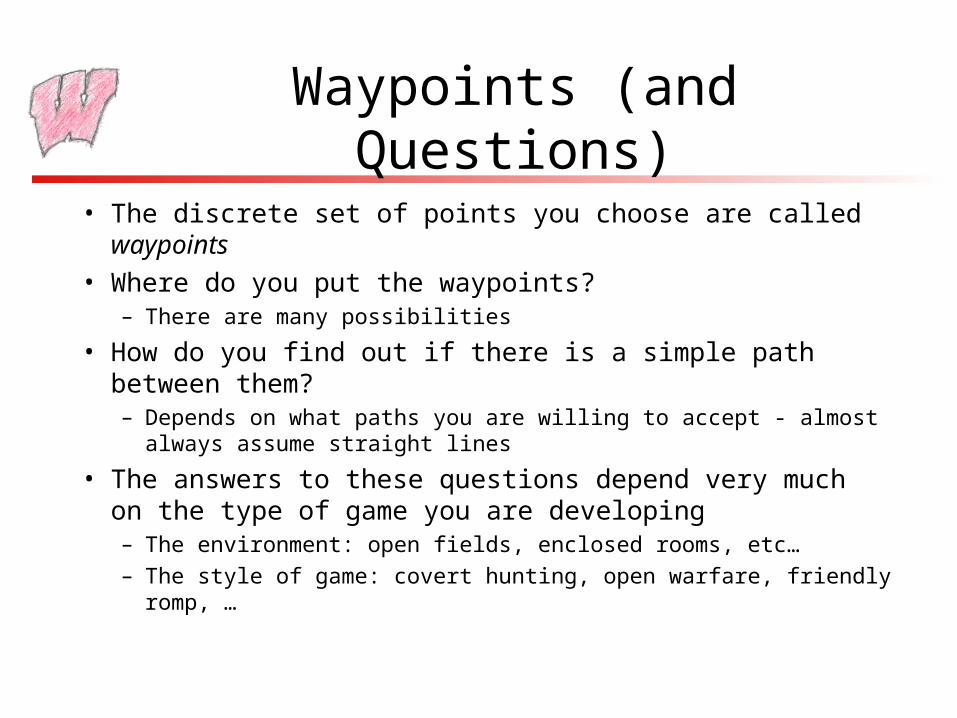
• The discrete set of points you choose are called waypoints

• Where do you put the waypoints?– There are many possibilities

• How do you find out if there is a simple path between them?– Depends on what paths you are willing to accept - almost always

assume straight lines

• The answers to these questions depend very much on the type of game you are developing– The environment: open fields, enclosed rooms, etc…

– The style of game: covert hunting, open warfare, friendly romp, …

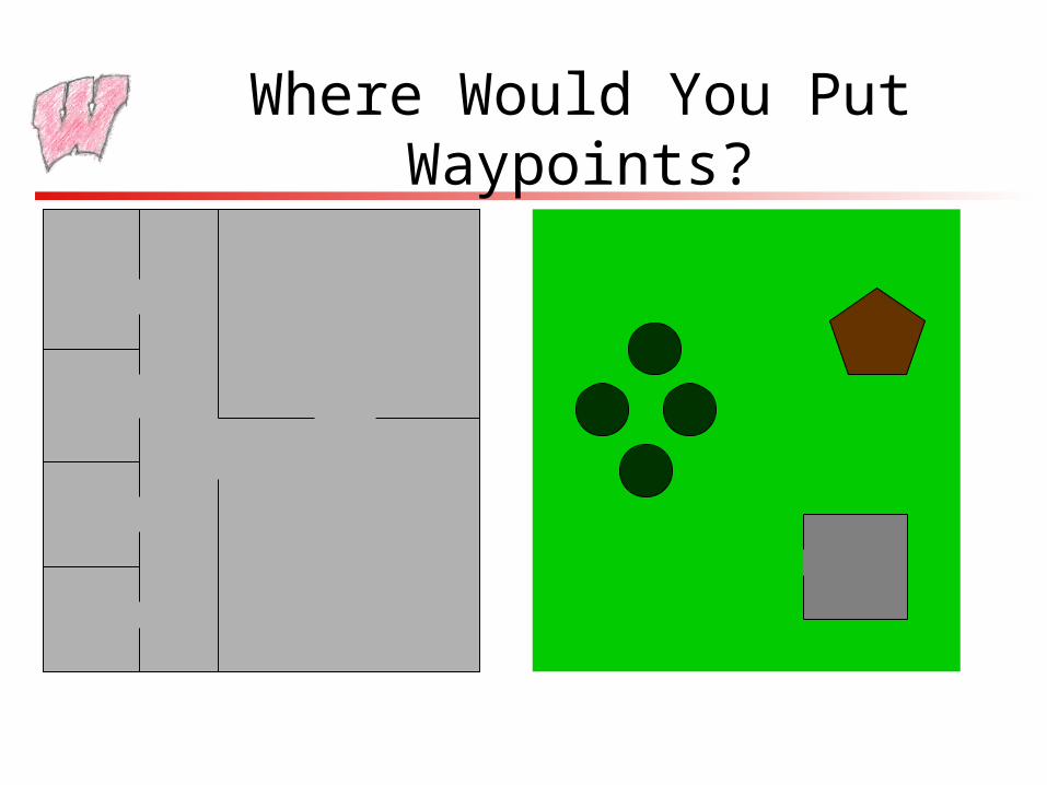
Where Would You Put Waypoints?

Waypoints By Hand

• Place waypoints by hand as part of level design– Best control, most time consuming

• Many heuristics for good places:– In doorways, because characters have to go through doors and

straight lines joining rooms always go through doors

– Along walls, for characters seeking cover

– At other discontinuities in the environments (edges of rivers, for example)

– At corners, because shortest paths go through corners

• The choice of waypoints can make the AI seem smarter

Waypoints By Grid

• Place a grid over the world, and put a waypoint at every gridpoint that is open– Automated method, and maybe even implicit in the environment

• Do an edge/world intersection test to decide which waypoints should be joined– Normally only allow moves to immediate (and maybe corner)

neighbors

• What sorts of environments is this likely to be OK for?

• What are its advantages?

• What are its problems?

Grid Example

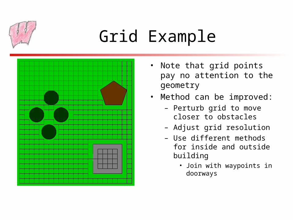
• Note that grid points pay no attention to the geometry

• Method can be improved:– Perturb grid to move closer to

obstacles

– Adjust grid resolution

– Use different methods for inside and outside building

• Join with waypoints in doorways

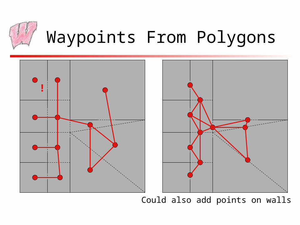
Waypoints From Polygons

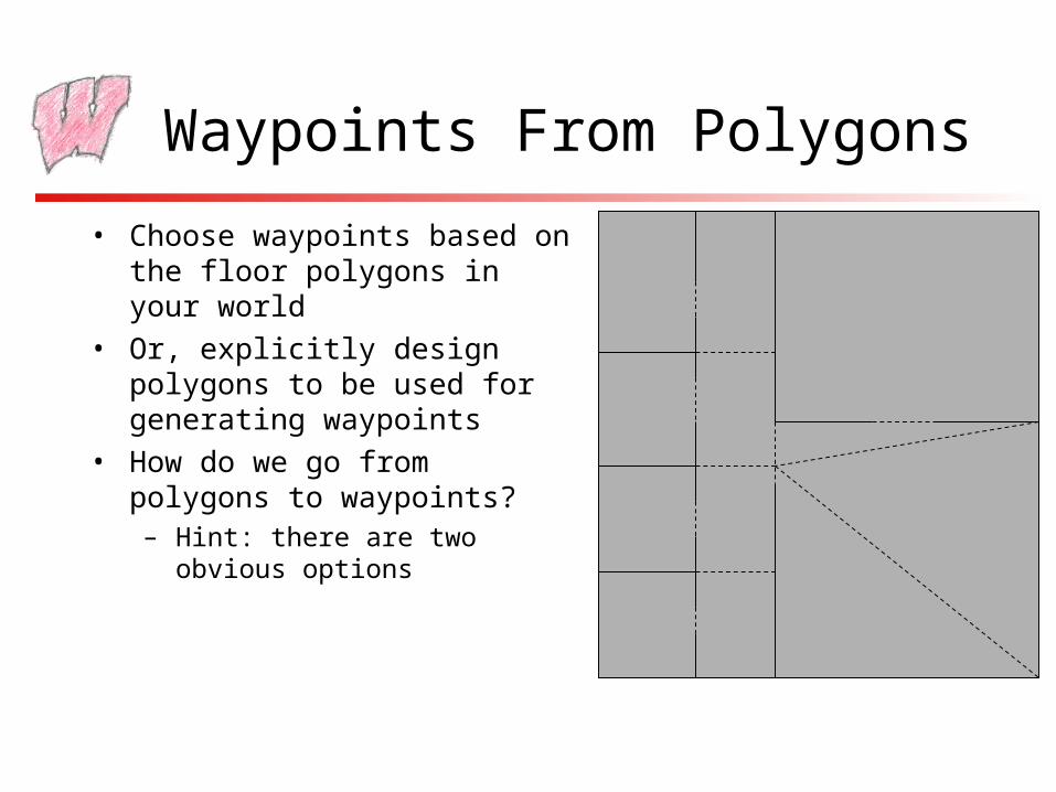
• Choose waypoints based on the floor polygons in your world

• Or, explicitly design polygons to be used for generating waypoints

• How do we go from polygons to waypoints?– Hint: there are two obvious options

Waypoints From Polygons

!

Could also add points on walls

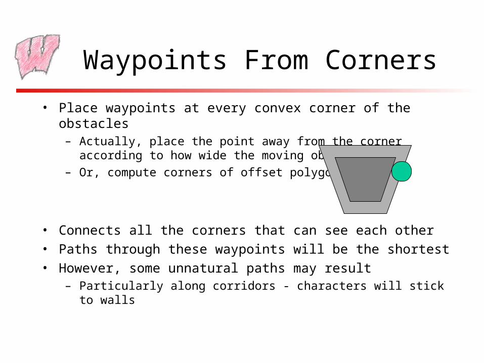
Waypoints From Corners

• Place waypoints at every convex corner of the obstacles– Actually, place the point away from the corner according to how wide the

moving objects are

– Or, compute corners of offset polygons

• Connects all the corners that can see each other

• Paths through these waypoints will be the shortest

• However, some unnatural paths may result– Particularly along corridors - characters will stick to walls

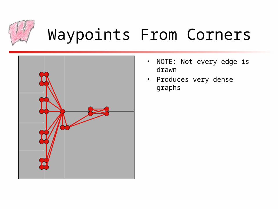
Waypoints From Corners

• NOTE: Not every edge is drawn

• Produces very dense graphs

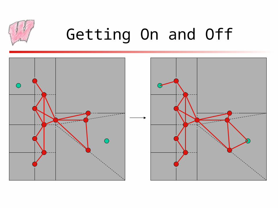
Getting On and Off

• Typically, you do not wish to restrict the character to the waypoints or the graph edges

• When the character starts, find the closest waypoint and move to that first– Or, find the waypoint most in the direction you think you need to go– Or, try all of the potential starting waypoints and see which gives

the shortest path

• When the character reaches the closest waypoint to its goal, jump off and go straight to the goal point

• Best option: Add a new, temporary waypoint at the precise start and goal point, and join it to nearby waypoints

Getting On and Off

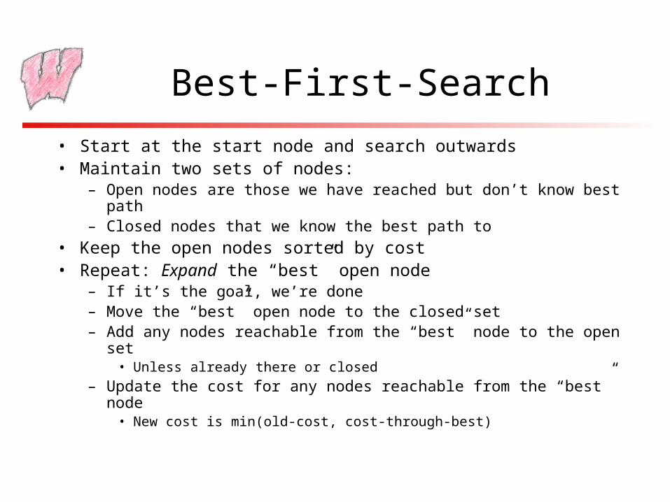
Best-First-Search

• Start at the start node and search outwards• Maintain two sets of nodes:

– Open nodes are those we have reached but don’t know best path– Closed nodes that we know the best path to

• Keep the open nodes sorted by cost• Repeat: Expand the “best” open node

– If it’s the goal, we’re done– Move the “best” open node to the closed set– Add any nodes reachable from the “best” node to the open set

• Unless already there or closed

– Update the cost for any nodes reachable from the “best” node• New cost is min(old-cost, cost-through-best)

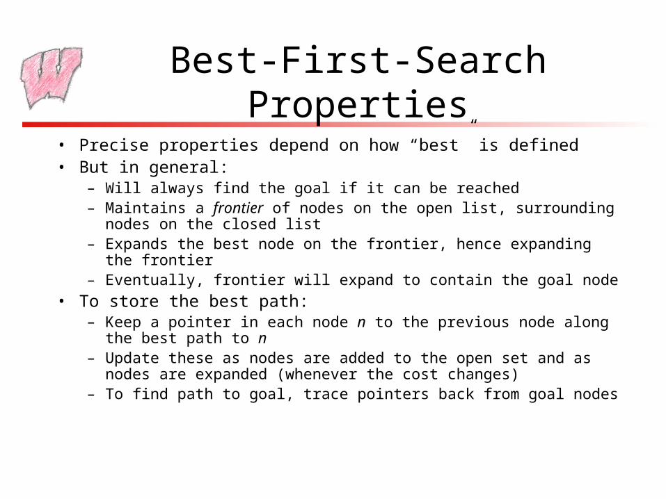
Best-First-Search Properties

• Precise properties depend on how “best” is defined• But in general:

– Will always find the goal if it can be reached– Maintains a frontier of nodes on the open list, surrounding nodes on the

closed list– Expands the best node on the frontier, hence expanding the frontier– Eventually, frontier will expand to contain the goal node

• To store the best path:– Keep a pointer in each node n to the previous node along the best path to n– Update these as nodes are added to the open set and as nodes are expanded

(whenever the cost changes)– To find path to goal, trace pointers back from goal nodes

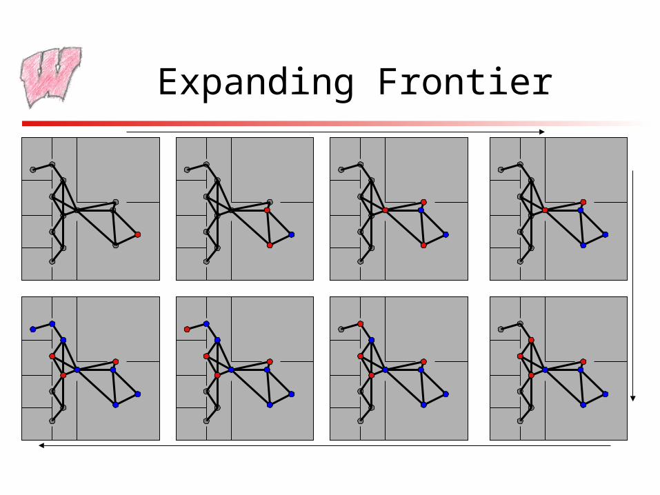
Expanding Frontier

Definitions

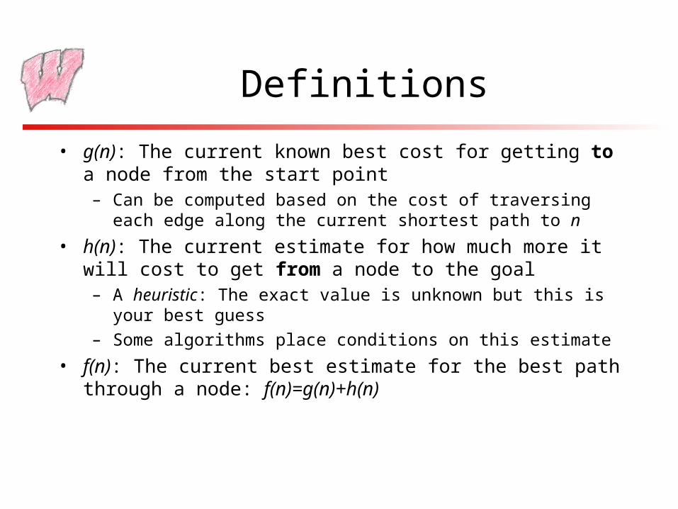
• g(n): The current known best cost for getting to a node from the start point– Can be computed based on the cost of traversing each edge along the

current shortest path to n

• h(n): The current estimate for how much more it will cost to get from a node to the goal– A heuristic: The exact value is unknown but this is your best guess

– Some algorithms place conditions on this estimate

• f(n): The current best estimate for the best path through a node: f(n)=g(n)+h(n)

Using g(n) Only

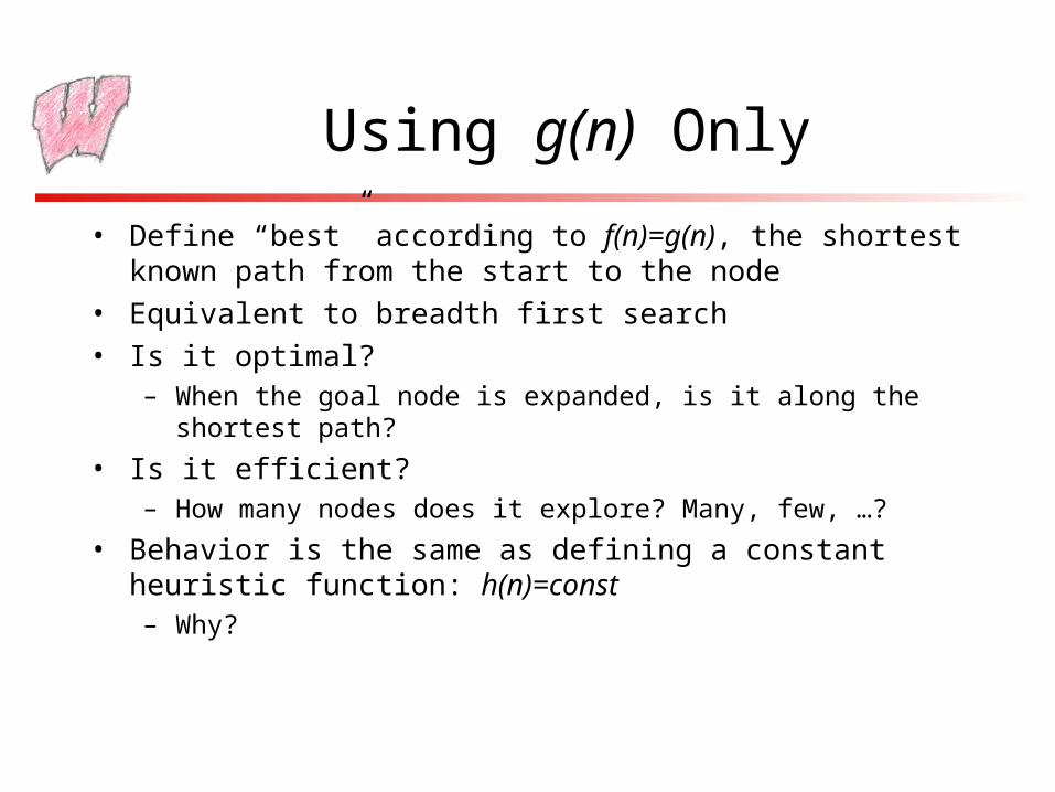
• Define “best” according to f(n)=g(n), the shortest known path from the start to the node

• Equivalent to breadth first search

• Is it optimal?– When the goal node is expanded, is it along the shortest path?

• Is it efficient?– How many nodes does it explore? Many, few, …?

• Behavior is the same as defining a constant heuristic function: h(n)=const– Why?

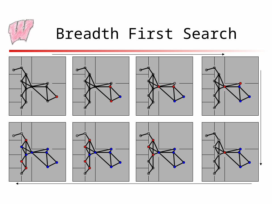
Breadth First Search

Breadth First Search

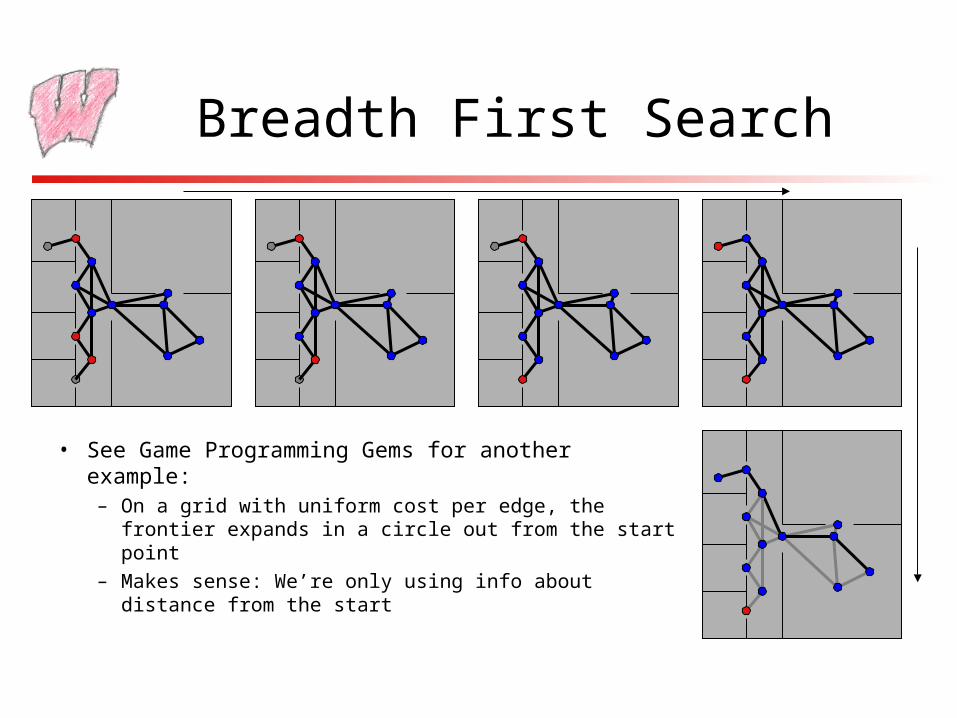
• See Game Programming Gems for another example:– On a grid with uniform cost per edge, the frontier

expands in a circle out from the start point

– Makes sense: We’re only using info about distance from the start

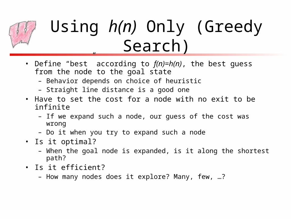
Using h(n) Only (Greedy Search)

• Define “best” according to f(n)=h(n), the best guess from the node to the goal state– Behavior depends on choice of heuristic– Straight line distance is a good one

• Have to set the cost for a node with no exit to be infinite– If we expand such a node, our guess of the cost was wrong– Do it when you try to expand such a node

• Is it optimal?– When the goal node is expanded, is it along the shortest path?

• Is it efficient?– How many nodes does it explore? Many, few, …?

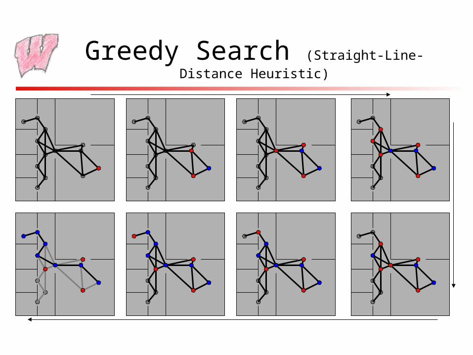
Greedy Search (Straight-Line-Distance Heuristic)

A* Search

• Set f(n)=g(n)+h(n)– Now we are expanding nodes according to best estimated total path cost

• Is it optimal?– It depends on h(n)

• Is it efficient?– It is the most efficient of any optimal algorithm that uses the same h(n)

• A* is the ubiquitous algorithm for path planning in games– Much effort goes into making it fast, and making it produce pretty looking

paths– More articles on it than you can ever hope to read

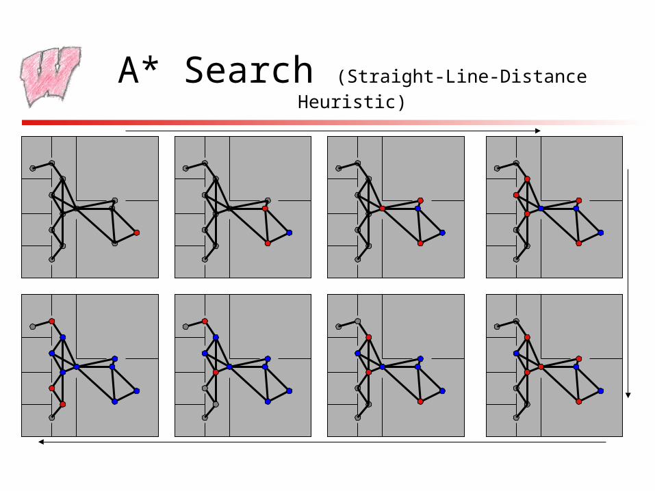
A* Search (Straight-Line-Distance Heuristic)

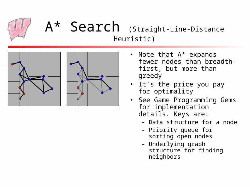
A* Search (Straight-Line-Distance Heuristic)

• Note that A* expands fewer nodes than breadth-first, but more than greedy

• It’s the price you pay for optimality• See Game Programming Gems for

implementation details. Keys are:– Data structure for a node– Priority queue for sorting open

nodes– Underlying graph structure for

finding neighbors

Heuristics

• For A* to be optimal, the heuristic must underestimate the true cost– Such a heuristic is admissible

• Also, not mentioned in Gems, the f(n) function must monotonically increase along any path out of the start node– True for almost any admissible heuristic, related to triangle

inequality– If not true, can fix by making cost through a node max(f(parent) +

edge, f(n))• Combining heuristics:

– If you have more than one heuristic, all of which underestimate, but which give different estimates, can combine with: h(n)=max(h1(n),h2(n),h3(n),…)

Inventing Heuristics

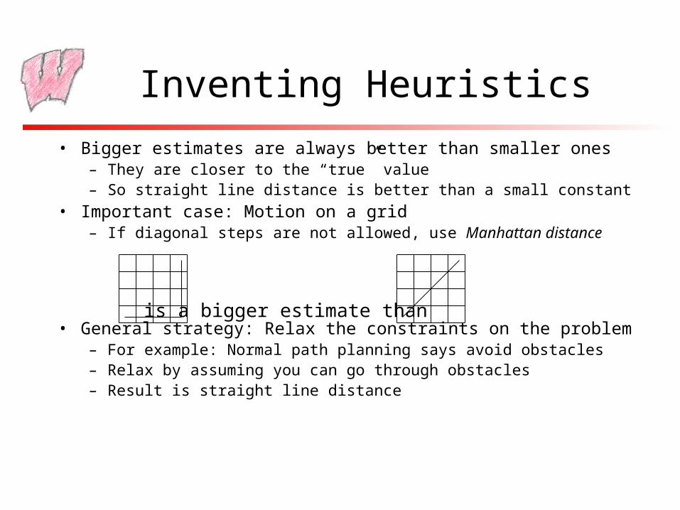
• Bigger estimates are always better than smaller ones– They are closer to the “true” value– So straight line distance is better than a small constant

• Important case: Motion on a grid– If diagonal steps are not allowed, use Manhattan distance

• General strategy: Relax the constraints on the problem– For example: Normal path planning says avoid obstacles– Relax by assuming you can go through obstacles– Result is straight line distance

is a bigger estimate than

Non-Optimal A*

• Can use heuristics that are not admissible - A* will still give an answer– But it won’t be optimal: May not explore a node on the optimal path

because its estimated cost is too high– Optimal A* will eventually explore any such node before it reaches

the goal• Non-admissible heuristics may be much faster

– Trade-off computational efficiency for path-efficiency• One way to make non-admissible: Multiply underestimate

by a constant factor– See Gems for an example of this

A* Problems

• Discrete Search:– Must have simple paths to connect waypoints

• Typically use straight segments

• Have to be able to compute cost

• Must know that the object will not hit obstacles

– Leads to jagged, unnatural paths• Infinitely sharp corners

• Jagged paths across grids

• Efficiency is not great– Finding paths in complex environments can be very expensive

Path Straightening

• Straight paths typically look more plausible than jagged paths, particularly through open spaces

• Option 1: After the path is generated, from each waypoint look ahead to farthest unobstructed waypoint on the path– Removes many segments and replaces with one straight one– Could be achieved with more connections in the waypoint graph,

but that would increase cost

• Option 2: Bias the search toward straight paths– Increase the cost for a segment if using it requires turning a corner– Reduces efficiency, because straight but unsuccessful paths will be

explored preferentially

Smoothing While Following

• Rather than smooth out the path, smooth out the agent’s motion along it

• Typically, the agent’s position linearly interpolates between the waypoints: p=(1-u)pi+upi+1

– u is a parameter that varies according to time and the agent’s speed

• Two primary choices to smooth the motion– Change the interpolation scheme

– “Chase the point” technique

Different Interpolation Schemes

• View the task as moving a point (the agent) along a curve fitted through the waypoints

• We can now apply classic interpolation techniques to smooth the path: splines

• Interpolating splines:– The curve passes through every waypoint, but may have nasty bends and os

cillations

• Hermite splines:– Also pass through the points, and you get to specify the direction as you go

through the point

• Bezier or B-splines:– May not pass through the points, only approximate them

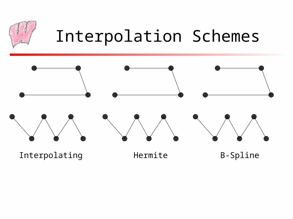
Interpolation Schemes

Interpolating Hermite B-Spline

Chase the Point

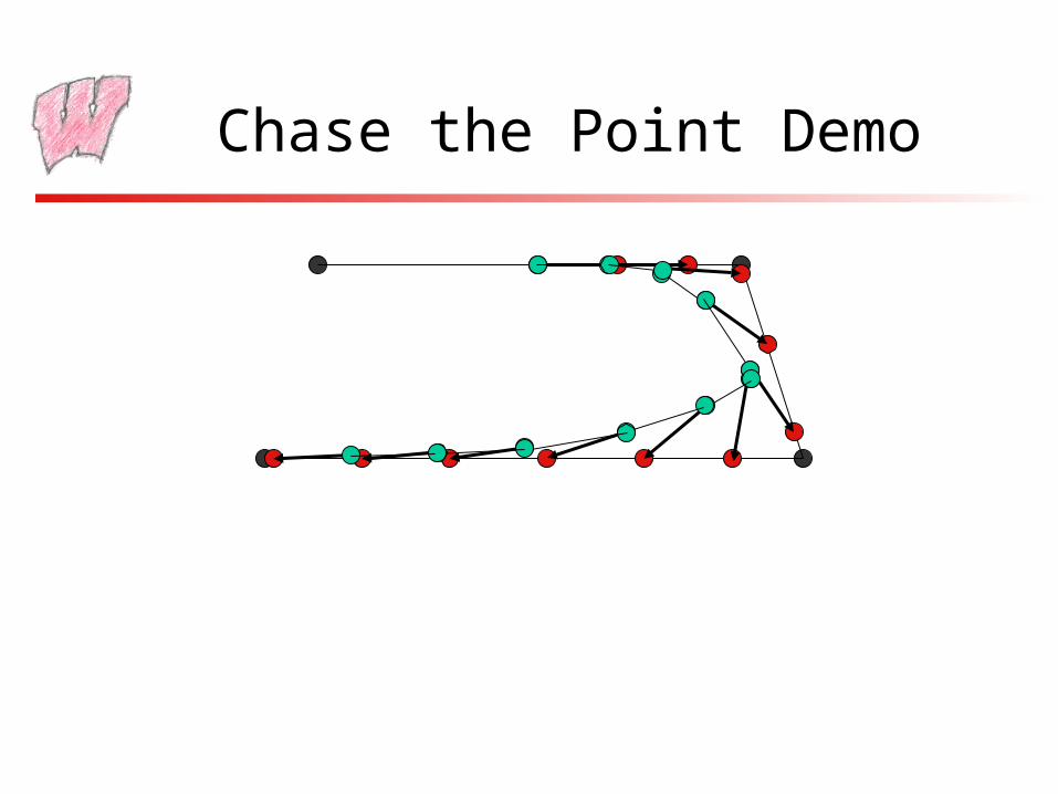
• Instead of tracking along the path, the agent chases a target point that is moving along the path

• Start with the target on the path ahead of the agent

• At each step:– Move the target along the path using linear interpolation

– Move the agent toward the point location, keeping it a constant distance away or moving the agent at the same speed

• Works best for driving or flying games

Chase the Point Demo

Still not great…

• The techniques we have looked at are path post-processing: they take the output of A* and process it to improve it

• What are some of the bad implications of this?– There are at least two, one much worse than the other

– Why do people still use these smoothing techniques?

• If post-processing causes these problems, we can move the solution strategy into A*

A* for Smooth Pathshttp://www.gamasutra.com/features/20010314/pinter_01.htm

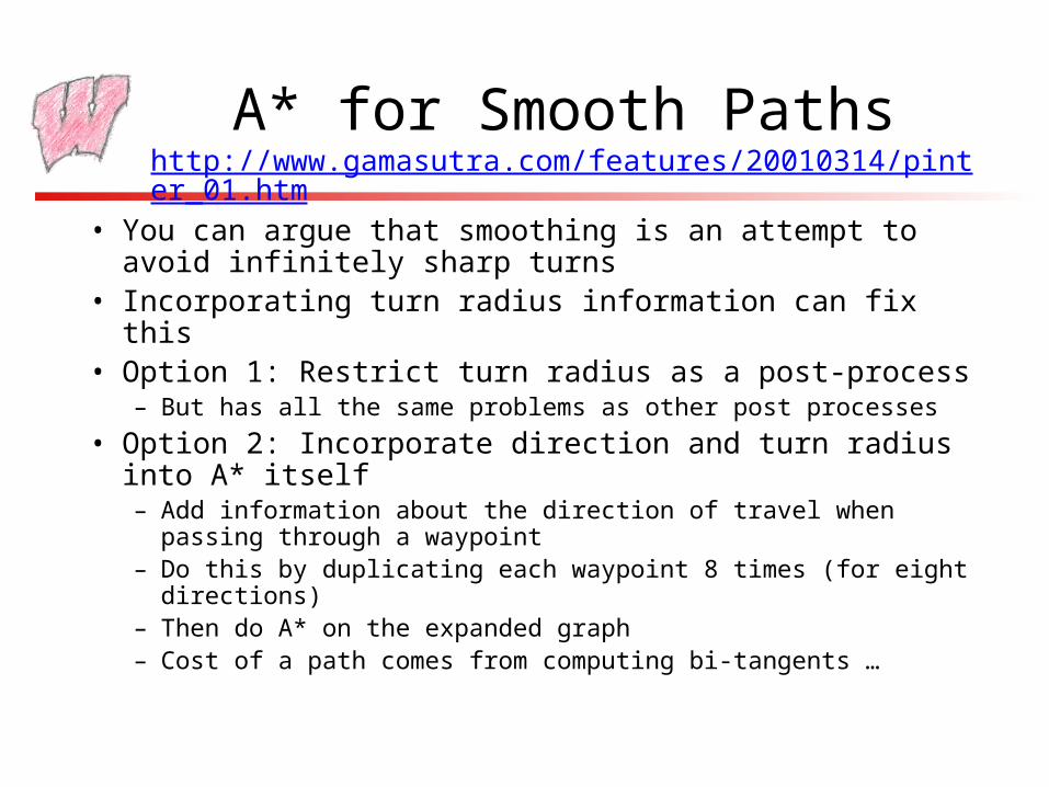
• You can argue that smoothing is an attempt to avoid infinitely sharp turns

• Incorporating turn radius information can fix this• Option 1: Restrict turn radius as a post-process

– But has all the same problems as other post processes

• Option 2: Incorporate direction and turn radius into A* itself– Add information about the direction of travel when passing through

a waypoint– Do this by duplicating each waypoint 8 times (for eight directions)– Then do A* on the expanded graph– Cost of a path comes from computing bi-tangents …

Using Turning Radius

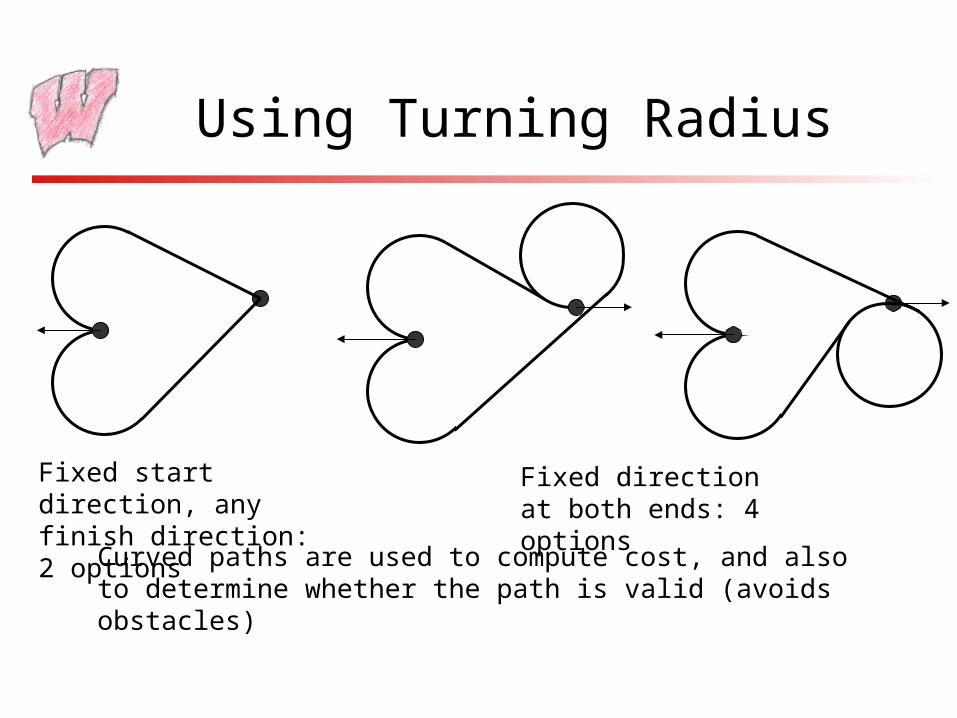
Fixed start direction, any finish direction: 2 options

Fixed direction at both ends: 4 options

Curved paths are used to compute cost, and also to determine whether the path is valid (avoids obstacles)

Improving A* Efficiency

• Recall, A* is the most efficient optimal algorithm for a given heuristic

• Improving efficiency, therefore, means relaxing optimality

• Basic strategy: Use more information about the environment– Inadmissible heuristics use intuitions about which paths are likely to

be better• E.g. Bias toward getting close to the goal, ahead of exploring early

unpromising paths

– Hierarchical planners use information about how the path must be constructed

• E.g. To move from room to room, just must go through the doors

Inadmissible Heuristics

• A* will still gives an answer with inadmissible heuristics– But it won’t be optimal: May not explore a node on the optimal path

because its estimated cost is too high

– Optimal A* will eventually explore any such node before it reaches the goal

• However, inadmissible heuristics may be much faster– Trade-off computational efficiency for path-efficiency

– Start ignoring “unpromising” paths earlier in the search

– But not always faster – initially promising paths may be dead ends

• Recall additional heuristic restriction: estimates for path costs must increase along any path from the start node

Inadmissible Example

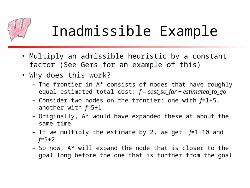
• Multiply an admissible heuristic by a constant factor (See Gems for an example of this)

• Why does this work?– The frontier in A* consists of nodes that have roughly equal

estimated total cost: f = cost_so_far + estimated_to_go

– Consider two nodes on the frontier: one with f=1+5, another with f=5+1

– Originally, A* would have expanded these at about the same time

– If we multiply the estimate by 2, we get: f=1+10 and f=5+2

– So now, A* will expand the node that is closer to the goal long before the one that is further from the goal

Hierarchical Planning

• Many planning problems can be thought of hierarchically– To pass this class, I have to pass the exams and do the projects

– To pass the exams, I need to go to class, review the material, and show up at the exam

– To go to class, I need to go to 1221 at 2:30 TuTh

• Path planning is no exception:– To go from my current location to slay the dragon, I first need to kn

ow which rooms I will pass through

– Then I need to know how to pass through each room, around the furniture, and so on

Doing Hierarchical Planning

• Define a waypoint graph for the top of the hierarchy– For instance, a graph with waypoints in doorways (the centers)

– Nodes linked if there exists a clear path between them (not necessarily straight)

• For each edge in that graph, define another waypoint graph– This will tell you how to get between each doorway in a single room

– Nodes from top level should be in this graph

• First plan on the top level - result is a list of rooms to traverse

• Then, for each room on the list, plan a path across it– Can delay low level planning until required - smoothes out frame

time

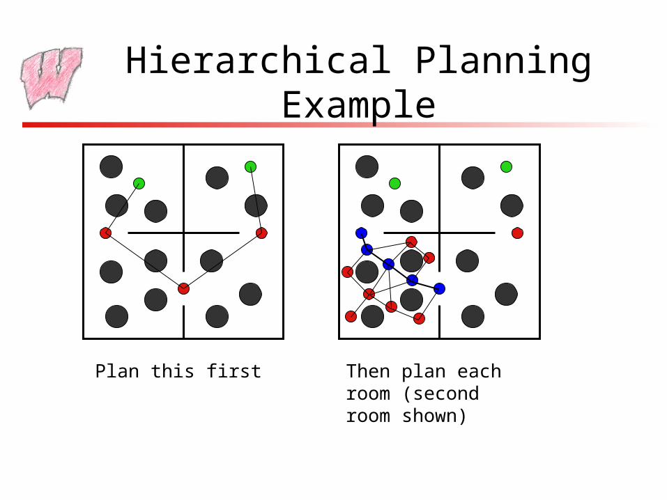
Hierarchical Planning Example

Plan this first Then plan each room (second room shown)

Hierarchical Planning Advantages

• The search is typically cheaper– The initial search restricts the number of nodes considered in the

latter searches

• It is well suited to partial planning– Only plan each piece of path when it is actually required

– Averages out cost of path over time, helping to avoid long lag when the movement command is issued

– Makes the path more adaptable to dynamic changes in the environment

Hierarchical Planning Issues

• Result is not optimal– No information about actual cost of low level is used at top level

• Top level plan locks in nodes that may be poor choices– Have to restrict the number of nodes at the top level for efficiency

– So cannot include all the options that would be available to a full planner

• Solution is to allow lower levels to override higher level– Textbook example: Plan 2 lower level stages at a time

• E.g. Plan from current doorway, through next doorway, to one after

• When reach the next doorway, drop the second half of the path and start again

Pre-Planning

• If the set of waypoints is fixed, and the obstacles don’t move, then the shortest path between any two never changes

• If it doesn’t change, compute it ahead of time

• This can be done with all-pairs shortest paths algorithms– Dijkstra’s algorithm run for each start point, or special purpose all-p

airs algorithms

• The question is, how do we store the paths?

Storing All-Pairs Paths

• Trivial solution is to store the shortest path to every other node in every node: O(n3) memory

• A better way:– Say I have the shortest path from A to B: A-B– Every shortest path that goes through A on the way to B must use A-B– So, if I have reached A, and want to go to B, I always take the same next

step– This holds for any source node: the next step from any node on the way

to B does not depend on how you got to that node– But a path is just a sequence of steps - if I keep following the “next step”

I will eventually get to B– Only store the next step out of each node, for each possible destination

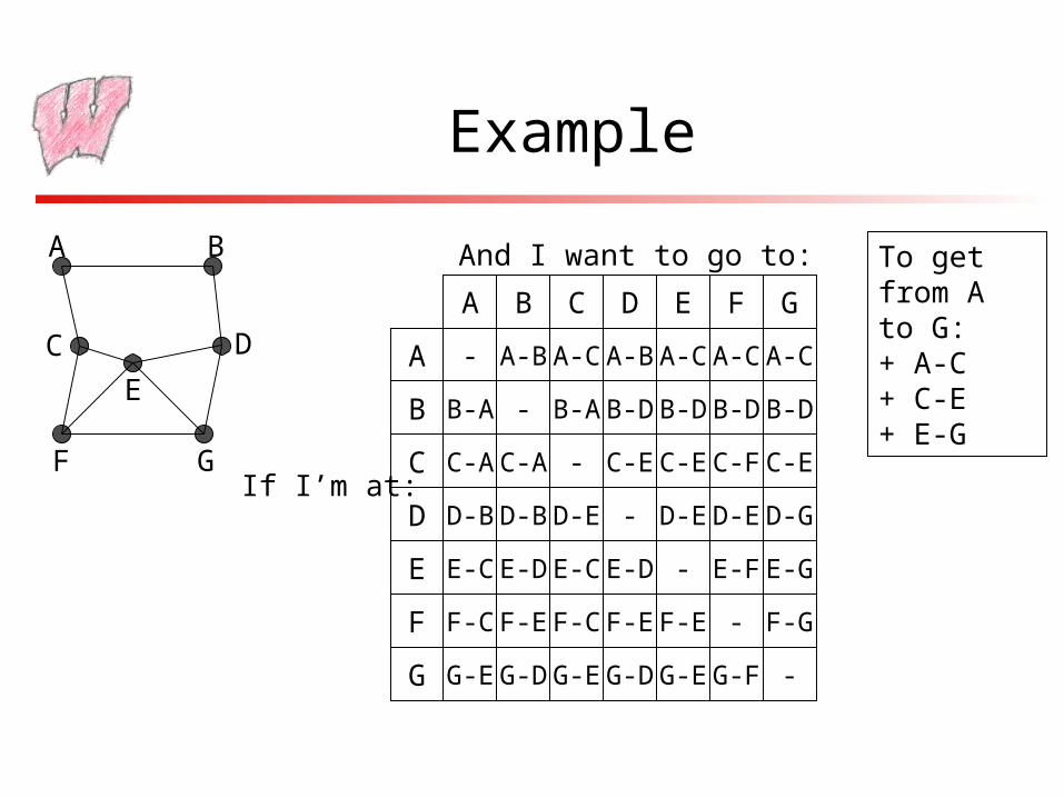
Example

A B

C D

E

F G

-

B-A

C-A

D-B

E-C

F-C

G-E

A

B

C

D

E

F

G

A-B

-

C-A

D-B

E-D

F-E

G-D

A-C

B-A

-

D-E

E-C

F-C

G-E

A-B

B-D

C-E

-

E-D

F-E

G-D

A-C

B-D

C-E

D-E

-

F-E

G-E

A-C

B-D

C-F

D-E

E-F

-

G-F

A-C

B-D

C-E

D-G

E-G

F-G

-

A B C D E F G

If I’m at:

And I want to go to: To get from A to G:+ A-C+ C-E+ E-G

Big Remaining Problem

• So far, we have treated finding a path as planning– We know the start point, the goal, and everything in between

– Once we have a plan, we follow it

• What’s missing from this picture?– Hint: What if there is more than one agent?

• What might we do about it?