TMD DISCUSSION PAPER NO. 65

A COMPUTABLE GENERAL EQUILIBRIUM

ANALYSIS OF MEXICO’S AGRICULTURAL POLICY REFORMS

Rebecca Lee Harris

International Food Policy Research Institute

Trade and Macroeconomics Division International Food Policy Research Institute

2033 K Street, N.W. Washington, D.C. 20006, U.S.A.

January 2001

TMD Discussion Papers contain preliminary material and research results, and are circulated prior to a full peer review in order to stimulate discussion and critical comment. It is expected that most Discussion Papers will eventually be published in some other form, and that their content may also be revised. This paper is available at http://www.cgiar.org/ifpri/divs/tmd/dp.htm

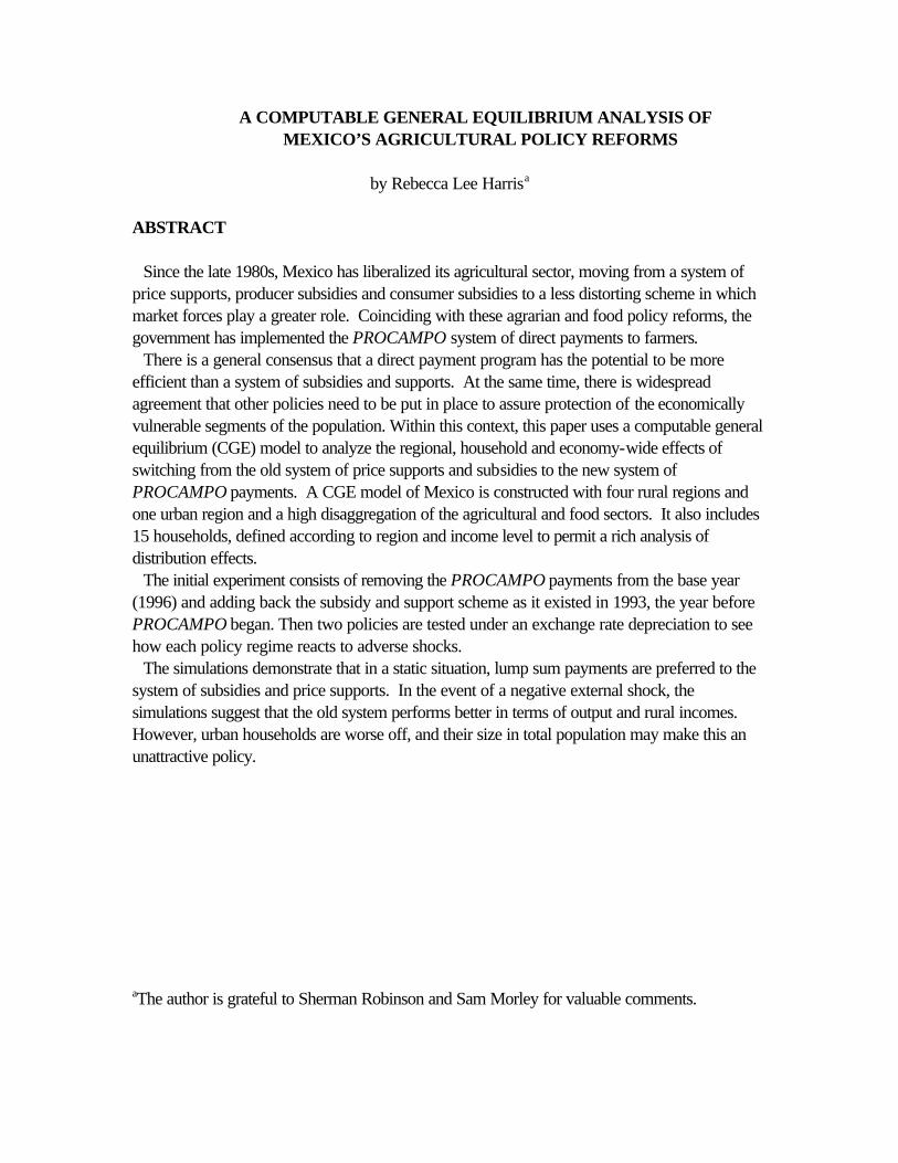
A COMPUTABLE GENERAL EQUILIBRIUM ANALYSIS OF MEXICO’S AGRICULTURAL POLICY REFORMS

by Rebecca Lee Harrisa

ABSTRACT Since the late 1980s, Mexico has liberalized its agricultural sector, moving from a system of price supports, producer subsidies and consumer subsidies to a less distorting scheme in which market forces play a greater role. Coinciding with these agrarian and food policy reforms, the government has implemented the PROCAMPO system of direct payments to farmers. There is a general consensus that a direct payment program has the potential to be more efficient than a system of subsidies and supports. At the same time, there is widespread agreement that other policies need to be put in place to assure protection of the economically vulnerable segments of the population. Within this context, this paper uses a computable general equilibrium (CGE) model to analyze the regional, household and economy-wide effects of switching from the old system of price supports and subsidies to the new system of PROCAMPO payments. A CGE model of Mexico is constructed with four rural regions and one urban region and a high disaggregation of the agricultural and food sectors. It also includes 15 households, defined according to region and income level to permit a rich analysis of distribution effects. The initial experiment consists of removing the PROCAMPO payments from the base year (1996) and adding back the subsidy and support scheme as it existed in 1993, the year before PROCAMPO began. Then two policies are tested under an exchange rate depreciation to see how each policy regime reacts to adverse shocks. The simulations demonstrate that in a static situation, lump sum payments are preferred to the system of subsidies and price supports. In the event of a negative external shock, the simulations suggest that the old system performs better in terms of output and rural incomes. However, urban households are worse off, and their size in total population may make this an unattractive policy. aThe author is grateful to Sherman Robinson and Sam Morley for valuable comments.

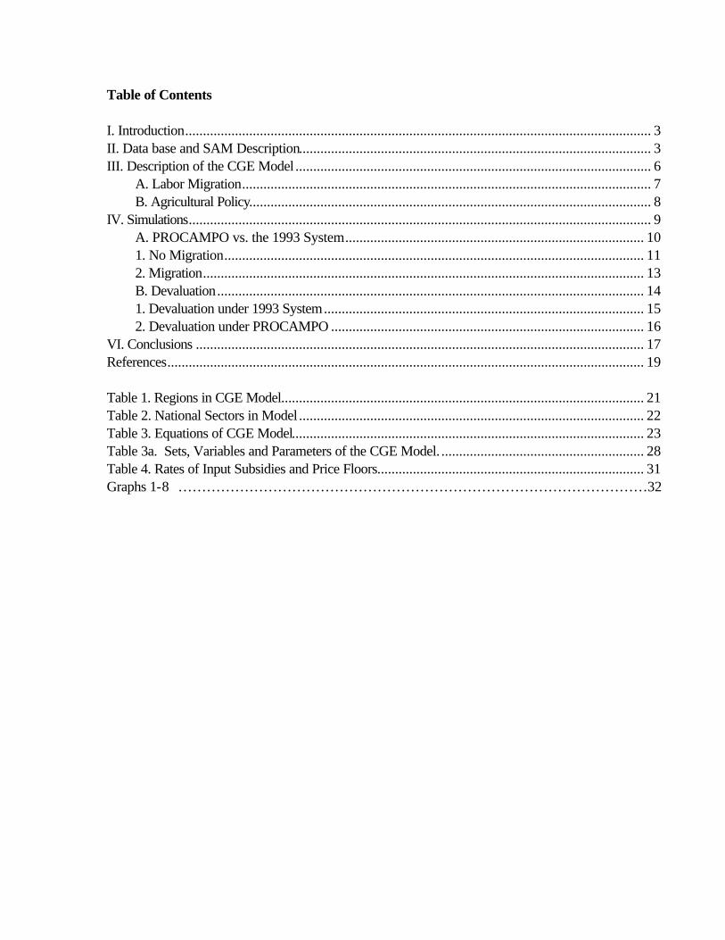
Table of Contents I. Introduction................................................................................................................................... 3 II. Data base and SAM Description................................................................................................... 3 III. Description of the CGE Model .................................................................................................... 6

A. Labor Migration................................................................................................................... 7 B. Agricultural Policy................................................................................................................. 8

IV. Simulations.................................................................................................................................. 9 A. PROCAMPO vs. the 1993 System.................................................................................... 10 1. No Migration...................................................................................................................... 11 2. Migration............................................................................................................................ 13 B. Devaluation........................................................................................................................ 14 1. Devaluation under 1993 System.......................................................................................... 15 2. Devaluation under PROCAMPO ........................................................................................ 16

VI. Conclusions .............................................................................................................................. 17 References...................................................................................................................................... 19 Table 1. Regions in CGE Model...................................................................................................... 21 Table 2. National Sectors in Model ................................................................................................. 22 Table 3. Equations of CGE Model................................................................................................... 23 Table 3a. Sets, Variables and Parameters of the CGE Model. ......................................................... 28 Table 4. Rates of Input Subsidies and Price Floors........................................................................... 31 Graphs 1-8 ………………………………………………………………………………………32

1

Introduction

Since the late 1980s, Mexico has liberalized its agricultural sector, moving from a system of price supports, producer subsidies and consumer subsidies to a less distorting scheme in which market forces play a greater role.1 Prior to the debt crisis of 1982, the economy was characterized by import substitution and trade protection and an active role of the State in the overall economy. The agricultural sector was also subject to heavy state intervention, with the objective of providing inexpensive and abundant food to the urban sector. A state-owned marketing agency, CONASUPO, was created in 1965 to purchase staple foods at artificially high producer prices and sell the final goods (ie. tortillas and bread) to consumers at artificially low consumer prices, with the government paying for the difference. In addition, poor urban families could receive free corn tortillas, while free milk was available to poor rural families. Farmers benefited not only from the CONASUPO price supports, but also from input and marketing subsidies as well as from import controls.

The 1982 debt crisis marked the turning point in Mexico's economic history, forcing the

government to re-think its traditional role in the economy.2 After a failed first attempt at structural adjustment in the mid-1980s, the government initiated the more comprehensive Economic Solidarity Pact in December 1987. The Pact included fiscal and monetary discipline, an incomes policy via a price and wage control agreement, public sector reform, and trade liberalization. The (unilateral) commitment to freer trade led to lower tariffs in all goods and the removal of import permit requirements for almost all agricultural commodities by 1989. At the same time, a new domestic agrarian reform program was announced, with the goal of reducing state intervention and increasing the role of agricultural markets. Since then, the state-owned agricultural agencies have greatly diminished in size and scope, including the phase-out of CONASUPO, and government involvement in price determination has been virtually eliminated. Other changes in agricultural policy included a major land reform of the ejido land tenure system,3 enacted in 1991, and the Alliance for Agriculture (Alianza para el Campo) program of 1995, which offers technical support to farmers.

A primary reform — and the focus of this paper — was the shift from distorting price

supports to direct payments to farmers. This 15 year program, known as PROCAMPO, was introduced in 1994 to gradually eliminate the price support policies for grains and oilseeds. To

1This section draws from OECD (1995) and various Attache Reports from the Foreign Agricultural Service of the U.S. Department of Agriculture.

2For a thorough background on the economic reforms following Mexico’s peso crisis of 1982, see Lustig (1998). 3See de Janvry, Gordillo and Sadoulet (1997) for a complete description and analysis of the ejido reform.

2

assist farmers with this price adjustment, they now receive PROCAMPO payments based on historical acreage of nine basic crops;4 since the payments are not based on current output levels, they are less distorting than the price supports. Although larger farmers will receive the greatest levels of support by definition, subsistence farmers who could not benefit from the price supports under the old system — because they did not market their production — are also able to access the payments. In fact, for the 1995 crop year, 88 percent of PROCAMPO recipients were farmers who owned less than five hectares of land, and they collected about half of the total payments. Subsistence farmers (cultivating less than two hectares and producing low-yield maize and beans) comprised 65 percent of eligible recipients and collected about a quarter of total payments.5

There is an extensive body of research on Mexican agricultural reforms, particularly in the

context of the North American Free Trade Agreement (NAFTA).6 While there is a general consensus that a direct payment program has the potential to be more efficient than a system of subsidies and supports, there is also widespread agreement that other policies need to be put in place to assure protection of the economically vulnerable segments of the population. Indeed, as Lustig (1998) observes, a primary reason why rural poverty increased after the 1994 peso devaluation (which in theory could help agricultural producers through increased exports), was that there were no social safety nets in place. Sadoulet, de Janvry and Davis (1999) recognize the potential multiplier effect of PROCAMPO payments, but show that this potential cannot be realized until liquidity constraints (such as weak property rights, poor access to rural credit) are resolved and technical assistance is provided to modernize agriculture.7

Although much of this literature comes on the heels of the 1994 crisis, very little has been

written about the extent to which the old system helped insulate rural

4These crops are: maize, wheat, beans, rice, sorghum, soyabeans, safflower, cotton and barley. 5It should be noted, as pointed out in Sadoulet, de Janvry and Davis (1999), that PROCAMPO is not a pure compensatory program, since all producers get paid at the same per hectare rate, regardless of their losses. Nor is it a pure welfare program, since PROCAMPO is not targeted specifically to poor farmers. Nonetheless, it provides a significant source of income to farmers, especially poorer ones. 6For a review of early studies on agriculture and NAFTA, see Josling (1992). 7This issue was raised before NAFTA’s implementation as well. Levy and van Wijnbergen (1992) suggest that the resources freed from price reform be used to enhance rural productivity through investments in land and irrigation systems. de Janvry, Sadoulet and Gordillo (1995) note similar concerns prior to NAFTA’s implementation, with a particular focus on the ejido sector.

3

households from external shocks vis a vis the new system.8 The paper will analyze the effects of switching from the system of price supports to the PROCAMPO payments in Mexico to examine two issues: (a) is the new system indeed more efficient than the old? and, (b) is the new system as effective as the old in protecting the rural poor from external shocks? These questions will be addressed in a computable general equilibrium (CGE) model, in order to analyze the regional, household and economy wide effects of the change in Mexico’s agricultural policy regime.

A CGE model of Mexico is constructed with four rural regions and one urban region and

a high disaggregation of the agricultural and food sectors. It also includes 15 households, defined according to region and income level. The model includes the PROCAMPO payments in the base year, which is 1996. The initial experiment consists of removing the PROCAMPO payments and adding back in the subsidy scheme as it existed in 1993, the year before PROCAMPO began. It is expected that the distortionary policies of 1993 will lower welfare under “normal” circumstances. However, this judgment may change if the economy is subjected to an external shock. Hence this study also tests the two policies under an exchange rate depreciation to see how each policy regime reacts. The CGE model permits an analysis of the two programs in terms of income distribution, welfare effects, rural versus urban impacts, and macroeconomic changes.

The next section describes the underlying data framework of the model, which comes

from a social accounting matrix (SAM) of Mexico. The third section describes the CGE model, with a particular focus on the distinguishing characteristics of the model. The agricultural policy simulations and their results are presented in section four. The final section makes some concluding remarks about the policy implications of the simulations. II. Data base and SAM Description The CGE model used in this analysis relies on a social accounting matrix (SAM) of Mexico, based on 1996 data.9 The SAM accounts for all income and expenditure transactions 8One exception is Burfisher, Robinson, and Thierfelder (2000), who view direct payments as an instrument for reducing risk, as well as a cushion against external shocks.

9The data used in constructing the SAM include: “Sistema de Cuentas Nacionales de México,” INEGI, 1998, for national accounts data and other macro data; Informe Anual, Banco de México, 1996 for macro data; SAGAR, 1996 for data on crop yields and land utilization; Encuesta Nacional de Ingresos y Gastos de Hogares, INEGI, 1994, for household income and expenditure data; GTAP database for import and export data. The input-output coefficients come from a 1985 input-output table. For a complete description of the SAM used in this model, see Harris (Forthcoming).

4

of all sectors and institutions in the national economy, and thus serves as the underlying data framework for the CGE model.10 The data were first collected as a national SAM, which was then divided into 5 regions. The model is able to capture differences among the regions in terms of production and consumption patterns, in a “top-down” approach: rather than having complete regional SAMs, the model regionally disaggregates production and factor markets as well as households.

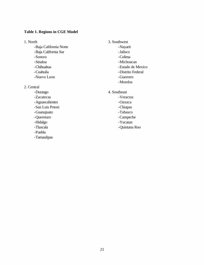
The model includes four rural regions, North, Central, Southwest and Southeast, which

produce only primary agricultural products.11 There is one “national” urban region, which comprises all of the urban areas of Mexico, regardless of geographical location. The urban area produces processed agricultural goods and other goods and services. Table 1 shows which states are in each rural region. Generally, the North region produces more high-valued agriculture, in particular fruits and vegetables, much of which is exported. Agriculture production relies on more irrigated land use, and households are wealthier. The Southeast region is poorest, more of the land used is non-irrigated, and there is less commercial farming. The Central and Southwest regions are a mixture of the first two, with a range of subsistence and commercial farming and agricultural technology. These two areas also produce the largest amounts of basic grains and beans.

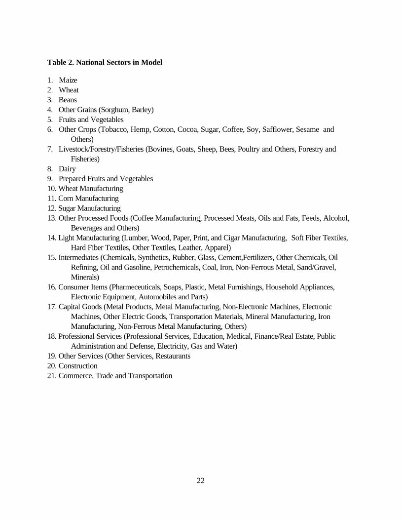
The SAM (and CGE model) permits the regionalization of agriculture. Each rural region produces 6 agricultural activities: maize, wheat, other grains, beans, fruits and vegetables, and other crops. The model allows for multiple production activities to produce one national commodity. For example, all four rural regions produce the maize activity, which is supplied to a single national maize commodity market. Thus there are 24 agricultural activities but 6 agricultural commodities. A given sector’s production is differentiated among the regions according to output levels and technology (in terms of factor and input usage). The livestock/forestry/fishery sector is not regionalized, due to data limitations. The urban region produces 15 goods, including processed agricultural goods, for a total of 39 activities and 21 commodities. Table 2 lists the sectors used in the model.

There are 4 types of non-agricultural labor: professional, white-collar, blue-collar, and unskilled/informal (referred to in this paper as unskilled), and four agricultural labor categories, differentiated by region. The agricultural activities only employ agricultural labor and non-agricultural activities do not use any agricultural labor. Each rural region uses two types of land, irrigated and non-irrigated, for a total of 8 land types. There is one capital category, used by all sectors. The model may be thought of as medium-term in nature, since labor and land are

10For a detailed discussion of SAMs, see Pyatt and Round (1985).

11The definition of "rural" used in this model is somewhat different from the standard. Here the urban-rural cutoff is set at 15,000 individuals.

5

mobile across sectors, but capital is not. Each region has 3 classes of households, defined as poor, medium or rich.12 The

delineation among categories comes from national data such that the poor are those in the lowest 40% income bracket of the entire country, regardless of location, the medium earn the next 40% of income and the rich households earn the top 20% of income. In this way, distributional impacts of different scenarios can be observed among income groups as well as among the regions. The rural regions get labor income from all labor types, distributed according to national survey data. Poor rural households receive 45% of the agricultural returns to dry land in their region, while medium rural households receive 55% of dry land income. All of the irrigated land payments go to the rich households. The land returns (to dry land) for the livestock/forestry/fishery sector are split among the medium and rich rural households. Rural households also receive capital income indirectly through enterprises. This income is calculated as the residual between income and expenditure. Urban households do not receive any income from agricultural labor; the other labor categories distribute payments to the households according to shares given in the national survey. Urban households do not receive any land income, and, like their rural counterparts, receive capital payments via the enterprise account.

Household consumption patterns also come from the survey data. Rural households have home consumption of the agricultural goods produced in their respective regions; all other goods are bought on the national market. All households save according to parameters estimated from household survey data.

The government and the enterprise account already alluded to are the other domestic institutions in the SAM. The government, which is national, collects seven types of taxes: a value-added tax, a producer tax, an export tax, a sales tax, an import tariff, a payroll tax and an income tax. It receives transfers from the rest of the world and provides transfers to households and enterprises. The rest of the world account provides transfers to households, buys Mexico’s exports, and sells its imports.

With the data for the SAM coming from so many disparate sources, it is not surprising that its initial construction was neither balanced nor consistent. The SAM was therefore balanced using maximum entropy techniques to incorporate prior knowledge in a consistent way.13

12Note that a household is defined as a family unit, therefore permitting a household to earn labor income from several labor categories.

13For discussion on this technique, see Robinson et al (2000).

6

III. Description of the CGE Model

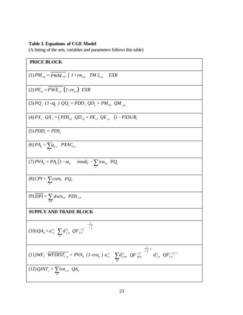
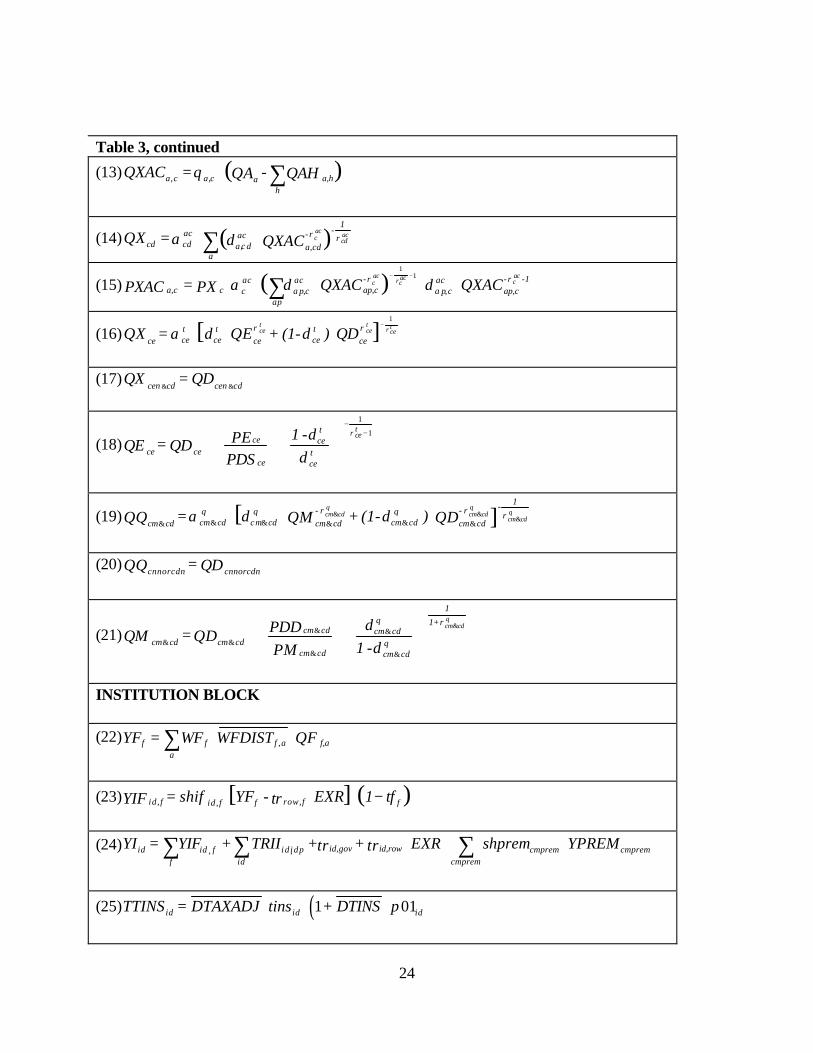
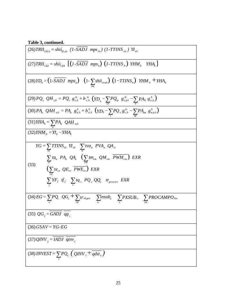
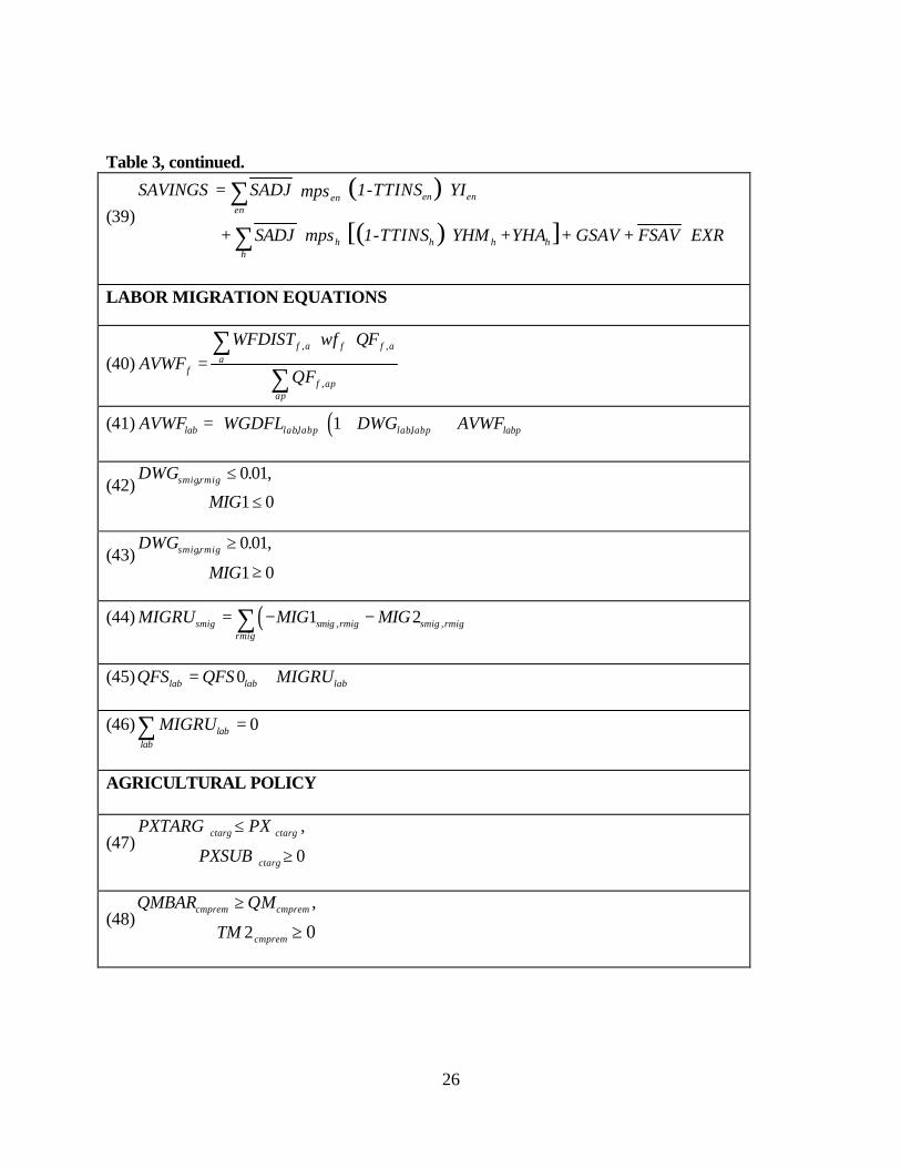
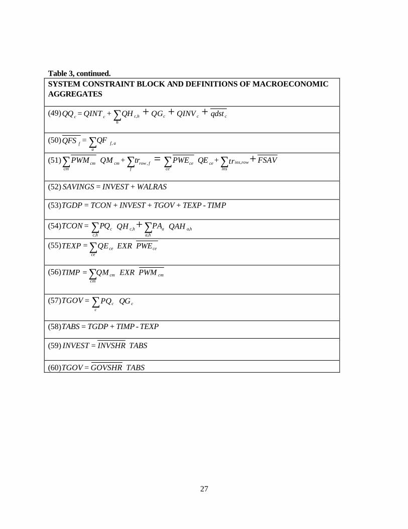
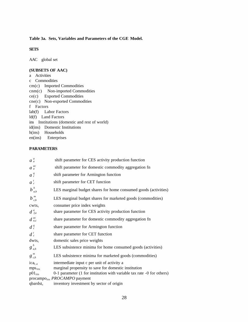
The computable general equilibrium model used in this study follows the sectoral and socioeconomic structure of the SAM described above. The CGE model is neo-classical in spirit, with agents responding to price changes. The model is Walrasian, determining only relative prices. Product prices, factor prices and the equilibrium exchange rate are defined relative to the consumer price index, which serves as the price numeraire. The country is “small” in the sense that it takes world prices as given. Following a general description of the standard features of the model, this section gives a more detailed explanation of some salient characteristics of the model: namely, labor migration behavior and the agricultural policy component. A complete listing of the model equations is presented in Table 3.

The production technology is a nested function of constant elasticity of substitution (CES) and Leontief functions. At the top level, domestic output is a linear combination of value added and intermediate inputs. Value added is a CES function of the primary factors of production (the land types, labor types and capital mentioned above) and intermediate input demand is determined according to fixed input-output coefficients. The commodity output is a composite of different activities, which are imperfectly substitutable: thus this framework allows multiple activities to produce one commodity, as discussed in the SAM description. Producers decide to supply their output to either the export or domestic market according to a constant elasticity of transformation (CET) function, which permits some degree of independence from international prices. The composite consumption good is a CES function of imported and domestically produced commodities. This aggregation, known as the Armington function, permits imperfect substitutability, and therefore, two-way trade, between imported and domestically produced goods.

Households receive income from factor payments (land, labor and capital payments) net of factor taxes, government transfers, and transfers from the rest of the world. They consume goods according to a linear expenditure function (LES), purchasing goods from the market as well as from home production (in rural areas only). They also pay taxes on their monetary income and save a share of their total income. Enterprises serve as the conduit between the capital factor account and the other institutions (households, government and rest of the world). They receive capital income minus capital payments to the rest of the world, as well as government transfers. Enterprises transfer that payment, net of depreciation and taxes, to households. Government income is the sum of all taxes: direct taxes on households and enterprises, value-added taxes, producer taxes, import tariffs, export taxes, social security taxes and sales taxes. The government consumes commodities according to fixed shares (given in the SAM) and also spends money on transfers to domestic institutions, and the three agricultural policies: the input subsidy, the price subsidy, and the PROCAMPO payment. Real government expenditure, real investment and foreign savings are all held fixed. Land and labor are mobile, while capital is sectorally fixed, to give the model a medium-term time horizon.

7

A. Labor Migration

The model is structured to allow labor migration between the rural regions and the urban region (in either direction), with a threshold effect of wage differences. Agricultural laborers from the four regions can migrate to the urban unskilled labor market and vice versa. Typically in CGE models a laborer's decision to migrate is based on the wage differential between what he is currently earning and what he would potentially earn if he moved. In this model, there are bounds on the earnings differential, inside of which the laborer will not move. This specification captures the fact that there may be a threshold effect on migration: it is likely that, within a range, changes in wages will not induce a laborer to move until the wage differential reaches some threshold.14 Migration can occur in both directions: if the wage differential between agricultural labor (in a given region) and the urban unskilled labor increases beyond a certain point, agricultural laborers will migrate out of their rural region. If the wage differential shrinks below a lower bound, unskilled laborers will migrate to the rural region. This model captures net flows of migration between any two regions and implicitly includes cross-region migration (for example, a migrant might move from his regional agricultural labor market to the urban labor market and from there to a different regional agricultural labor market).

As seen in Table 3, the equations for labor migration are set up as a mixed-

complementarity problem, in which the wage differentials are written as inequalities and linked to the migration variables in complementarity slackness conditions. Equation (40) defines the initial average wage of a factor as the total payment to the factor across sectors divided by the total supply of the factor. Equation (41) describes the relationship between the wages of two different labor categories: the initial average wage in one labor category15, AVWFlab, is equal to a wage differential, WGDFLlab,labp, plus a bounded variable, DWGlab,labp, multiplied by the initial average wage in the other labor category. In these simulations, the comparison is between the 14While this analysis does not explicitly take into account expected wages, as in a Harris-Todaro framework, or any other factors of the migration decision, such as preferences, urban crowding, distance from family, etc., these may be implicitly captured by the threshold effect. It should also be noted that this study assumes that potential migrants only look at returns to the margin, and so the PROCAMPO payments will not affect the decision to migrate. In reality, the effect is ambiguous. If potential migrants view the payment as a guaranteed source of income, then they might be more likely to leave the farm for an urban sector (or U.S.) job. On the other hand, if agricultural workers regard the payment as a support to their agricultural wages, then they may be more likely to stay on the farm. See Burfisher, Robinson and Thierfelder (1994) for different treatments of the relationship between transfers and migration.

15In this study, agricultural labor is defined by region, thus “labor category” refers to the set of labor types including four separate agricultural labor types, one from each rural region.

8

agricultural wage of a given region and the urban unskilled wage. In the base, DWGlab,labp equals zero by assumption and there is no migration. If, as a result of a simulation, the wage differential changes, then DWGlab,labp will also change in the opposite direction to keep the equation balanced. For example, suppose initially the average agricultural wage is 1.0 and the average unskilled labor wage is 2.5. Thus the wage differential ratio is 0.4. Now, if there is an increase in unskilled wages to 3.0, the ratio falls to 0.33. DWGlab,labp will now equal -0.17 in order to maintain the equality of the initial average wages.

Equations (42) and (43) further elaborate on the bounds for DWGlab,labp. Here it is set

to be between -0.01 and +0.01, which, in this setting, can be thought of as a one percent change (positive or negative) in the wage differential ratio. The complementary slackness conditions for these equations are also presented, showing that as long as DWGlab,labp remains within its bounds, migration will be zero. If DWGlab,labp hits either of the bounds, then there will be migration. If DWGlab,labp reaches -0.01, there will be positive migration out of the rural area. If the wage differential increases, DWGlab,labp compensates by becoming negative. If it reaches the bound, the wage differential has grown enough to induce migrants to leave the rural region. Similarly, if DWGlab,labp reaches +0.01, this signifies that the wage differential has reached a threshold that induces urban migrants to move to the rural region.

Equation (44) adds up all of the migrants that could enter or leave a labor market.

Equation (45) adds (or subtracts) that figure from the total labor supply of the category, to get the new labor supply after migration. Equation (46) ensures that the net sum of migration among categories is zero. If there is a positive migration from the rural area to the urban area, there is “negative” migration from the urban area to the rural area. Of course, in this analysis, there are four rural areas, so the sum of the rural migration should equal the negative sum of urban migration. B. Agricultural Policy

In this study, two specific agricultural policies are modeled: price supports for producers

of four agricultural commodities (Maize, Wheat, Beans, and Other Grains) and input subsidies on all agricultural activities. Consumer subsidies are implicitly included as an input subsidy: producers of processed goods - Wheat Flour, Maize Flour, and Dairy Manufacturing - receive a subsidy, which lowers the price to consumers. The input subsidy is used as an instrument which lowers the cost of production and is included in the value-added price equation (equation 7). The price support is modeled using the MCP specification to allow for inequalities and a complementary slackness variable: if the price of the targeted commodity falls below the given floor, then the government pays a subsidy to support the price. A third policy must be included in order to make the price floor comport with government goals; namely, an import quota must be instated for goods subject to the price floor. Otherwise, imports will further depress the price of these goods. This policy is also modeled as a mixed-complementarity problem, since the import quota will only "kick in" if there is an increase in

9

pressure to import (relative to the base).

The equations for these policies are described in Table 3. In equation (47), the price target, PXTARGctarg, is defined over the set of targeted commodities, ctarg. PXctarg, which is the output price for both domestically sold and exported goods, must be greater than or equal to the target price. As long as PXctarg exceeds the floor price, the linked variable, PXSUBctarg, representing the government subsidy rate, is zero. If there is downward pressure on PXctarg such that it equals the lower bound, PXTARGctarg, then the government pays the subsidy to support the price, and PXSUBctarg becomes positive. Note that PXSUBctarg is also included in the definition of PXc (equation (4)), lowering the output price, and PXSUBctarg must be accounted for in the equation on government expenditures (equation (34)), in which the government pays the subsidy for each unit QX which is marketed.

The import rationing scheme is described by equation (48). Defined over all rationed

commodities, cmprem, in this model, it restricts imports as follows. Imports, QMcmprem cannot exceed the targeted amount, QMBARcmprem, which is set at the base level. If QMcmprem equals the bound, the import premium, TM2cmprem, becomes positive. TM2cmprem is also added into equation (1), describing the price of imports. In addition, an equation must be included in the model to collect the import premium, seen in equation (49). The premium income, YPREM, is equal to the premium, times the level of imports, times the price of imports. YPREM must then be included the equation for institutions' incomes (equation (24)). IV. Simulations

The base year of the CGE model is 1996. In this year, PROCAMPO payments were in

effect for eligible rural households and most of the dismantling of the agricultural price supports and subsidies had been accomplished. The simulations presented here compare the 1996 status quo with the system of agricultural protection from 1993, the year before PROCAMPO started. In the runs which include the policies from 1993, the PROCAMPO payment is removed, and the equations for the agricultural policies described in the previous section are implemented. In particular, a price floor is effective for Maize, Wheat, Beans and Other Grains, and these goods are also subject to an import quota. In addition, all raw agricultural activities (Maize, Wheat, Beans, Other Grains, Fruits and Vegetables, and Other Crops — for each region — and Livestock) and three processed agricultural activities (Dairy, Wheat Manufacturing and Maize Manufacturing) receive input subsidies.16 The amounts of the protection are given

16Input subsidies refer to two types of distorting subsidies according to the OECD (1995): (1) "Reduction of input costs," including capital grants, interest concessions, and reductions on the costs of irrigation, feed, breeding improvement, seeds and machinery. This is applied to all crops, livestock and dairy. (2) Dairy, Wheat Manufacturing and Corn Manufacturing also receive subsidies on the purchase price of raw intermediate goods, which as mentioned earlier, represent the consumer subsidies.

10

in Table 4. These numbers were calculated based on the relative amounts compared to 1996, since not all of the policies were fully dismantled in that year.

The first simulation starts from the base-run of the 1996 model, in which the PROCAMPO payments are in place and most of the agricultural subsidies and supports have been reduced substantially. Then the system of subsidies and supports as they existed in 1993 is added to the model, while removing the PROCAMPO payments, to get a general idea of how the economy was prior to liberalization. This simulation is done first without allowing for migration, to get a clearer understanding of the mechanics of the systems, and then it is performed with internal migration. The next section evaluates the two programs under an exchange rate devaluation, to see the different ways that the economy reacts. For ease of presentation, the system of price supports and subsidies will be referred to as the "1993 system."

The simulations performed by the CGE model result in counterfactual equilibria which

can be compared to the base run equilibrium. In this analysis, the equivalent variation (EV) measure is used to see how each household’s welfare changes in the different scenarios. This study will also pay attention to changes in real income for each household, which do not necessarily move in tandem with EV. For example, if an exogenous change raises a household’s income but also induces inefficient consumption, EV will be negative. Income changes are also useful to trace the second-round effects of an exogenous change. Complementing the effects on income and EV are the effects on wages and the factor markets.

In all of the experiments, real government expenditure, real investment and foreign

savings are all held fixed. Thus all changes in absorption come from changes in consumption. The government budget is kept neutral, so that the government surplus or deficit does not need to be added into the welfare analysis.17 A. PROCAMPO vs. the 1993 System

The removal of distorting subsidies and price floors is expected to have an expansionary

effect on the economy as a whole: switching to the PROCAMPO system should lead to a more efficient allocation of resources by consumers and producers. Within the agricultural regions, production should move away from the protected products and toward the other crops. The move to a more efficient composition of agricultural production should cause agricultural wages to fall, leading to rural-urban migration. All in all, welfare should fall for rural dwellers, who get lower incomes and pay more for food products, and it is expected to rise for urbanites, whose income sources increase and who spend relatively smaller portions of their budget on food anyway.

17Otherwise, a program may look welfare enhancing to a household without considering the ramifications of increased an government deficit.

11

1. No Migration

The first simulation set compares the PROCAMPO scenario with the system of price

supports and subsidies. The 1993 system is more costly than the PROCAMPO program (raising the government deficit from 12 billion pesos to over 62 billion), so the difference is made up by raising the income tax rate proportionately for all households. The income tax may be thought of as lump-sum (ie., non-distorting) in nature, since there is no explicit modeling of leisure in the model. In the initial run, the experiment does not allow for migration, in order to more easily sort out the effects of the policy changes, and then migration is put in as well.

The PROCAMPO policy has a slightly expansionary effect on the macroeconomic indicators compared to the 1993 system, with real GDP and absorption rising by over 1 percent. This leads to an appreciation of the exchange rate. Due to the closure rules, real government spending, real investment and foreign savings stay fixed.

Because this simulation has many components changing simultaneously, it is useful to

inspect the effects of each instrument independently before proceeding with the full analysis of the sectoral changes. First, the effect of removing the input subsidy on domestic supplier prices (PDc) is ambiguous if it is imposed on more than one product. If the subsidy is only removed from the raw agricultural activities (ie., Maize, Wheat, etc.), then the resulting outcome is straightforward: the higher cost of production leads to a higher producer price, which translates into a higher commodity price. This also harms the processed good associated with the protected raw good (ie., Maize Manufacturing and Wheat Manufacturing). However, if the subsidy is also removed from processed food activities, as is the case in this study, then the processed good demands less of the raw product as an intermediate good. The net result is that the raw good experiences an decrease in its price, even though it has been harmed from the removal of the input subsidy. The processed goods (Maize Manufacturing, Wheat Manufacturing and Dairy) do experience price rises due to the removal of their input subsidies.

In the 1993 simulation, the price floor is specifically imposed on the average output

price (PXc) of Maize, Wheat, Beans, and Other Grains.18 When the price floor is removed for the PROCAMPO experiment, it lowers PXc on these goods as well as on all other agricultural goods. The reshuffling of output which results from removing the price floor leads to a more efficient reallocation of agricultural factors (ie., agricultural labor and land) which lowers the prices of those factors. Thus all raw goods which use agricultural factors face lower factor costs, which leads to the activity price decreases. In the absence of other policies, the good which is harmed from the price floor removal decreases its production as a result, which may

18Recall that this policy is accompanied by import rationing for the affected commodities.

12

drive up the domestic producer price (PDc). Since this translates into a higher composite commodity price (PQc), the processed activities which use that good as an intermediate input will face higher costs and thus a higher activity price (PAa).

When these two policies — the input and producer subsidies and the price floor— are

jointly removed from the above mentioned products, all raw agricultural products experience decreases in their output price. However, only Maize and Wheat decrease in production. Their rates of protection in the 1993 system are higher than those of the other raw goods (and their demands as intermediate products are greater) so when the protectionary instruments are removed, resources flow away from these two crops toward the other crops. The reaction of the composite commodity price, depends on the interaction of supply and demand.19 In the case of Maize, the price rises because of a shortage, but the other crops' prices decrease. Of the processed goods, Manufactured Wheat and Manufactured Corn decrease in output, because less of the raw good is available to them and their subsidies disappear. Their output prices and composite commodity prices increase, as their input subsidies are removed. All other processed goods increase in output because of the increase in production of their respective intermediate goods.

In terms of regional impact, the switch to the PROCAMPO policy lowers output in the Maize and Wheat sectors everywhere, since these are the products with the greatest producer price decreases. In this full employment model, these decreases imply that some regions will get a boost in their production of other goods, including other sectors whose protection has been removed. For example, in the Southwest and Southeast, Bean production rises, and Other Grains production increases everywhere. The crops which did not receive protection from the price floor, namely, Fruits and Vegetables and Other Crops, also experience increases in output. In the urban regions, Wheat Manufacturing and Maize Manufacturing suffer from the decreases in the raw outputs, but other processed goods sectors ultimately raise production due to the increases in their raw inputs. Overall, this reallocation of production, combined with the positive effects of an appreciation of the exchange rate on non-tradables, causes urban production to improve.

On net, total agricultural production rises because of the more efficient reallocation of

resources. The reshuffling of production causes downward pressure on all agricultural factor prices. Agricultural labor wages fall in all regions, from 20% in the Central region to 27% in the Southeast over the base. Dry land returns decrease everywhere, from 30% in the Southeast to 47% in the Southwest, reflecting the dry land intensity of the formerly protected crops. Irrigated land decreases in value in all but the Southeast region, the one region in which Wheat (which is irrigated land intensive) actually increases in output. The general expansion of urban production causes all urban labor categories to experience slight increases in wages. Professional and white

19The composite commodity price, PQc, will also be affected by the import price — depending on the Armington elasticities. However, the directional changes still follow those of PDc.

13

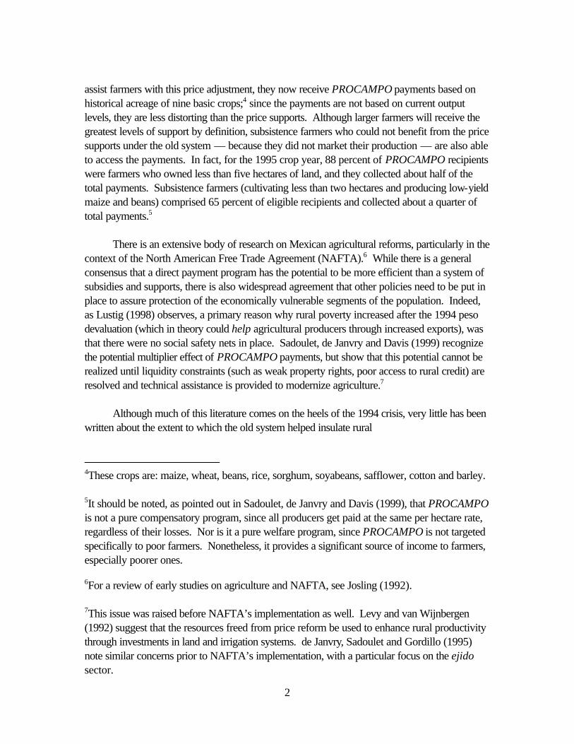
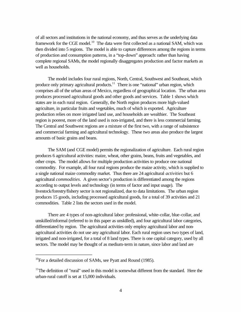
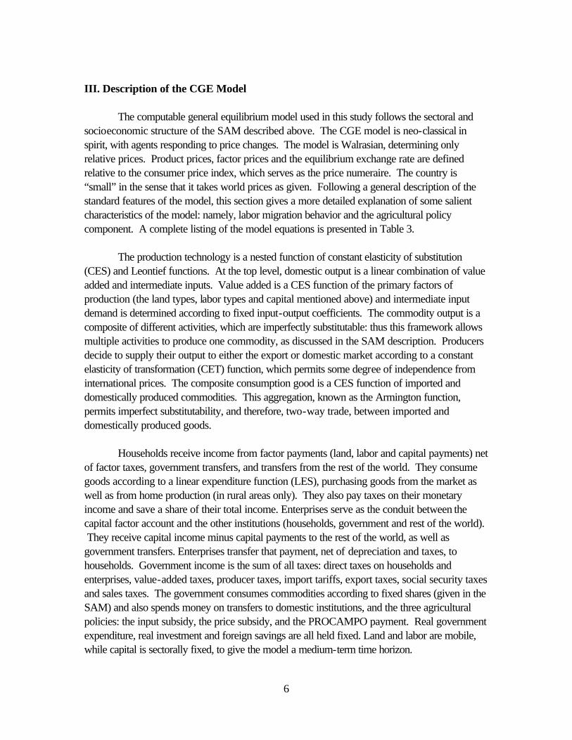
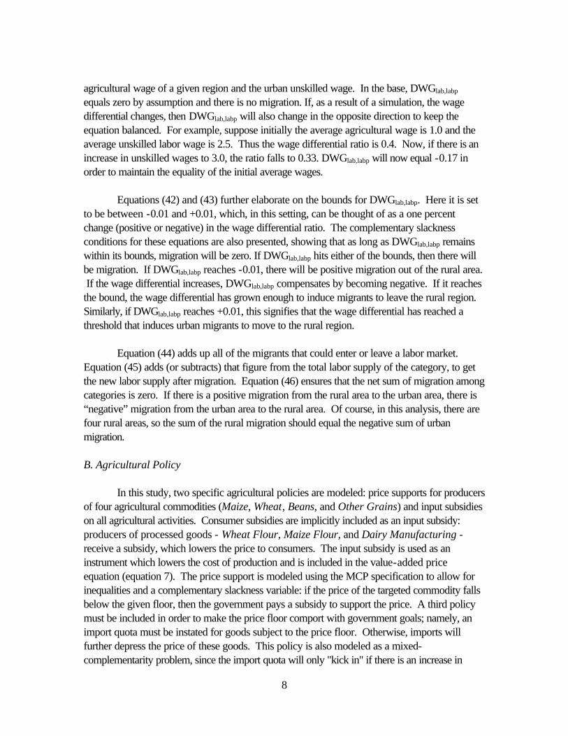
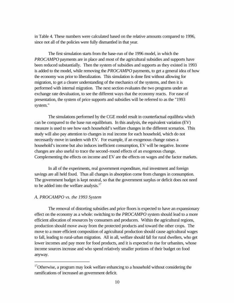
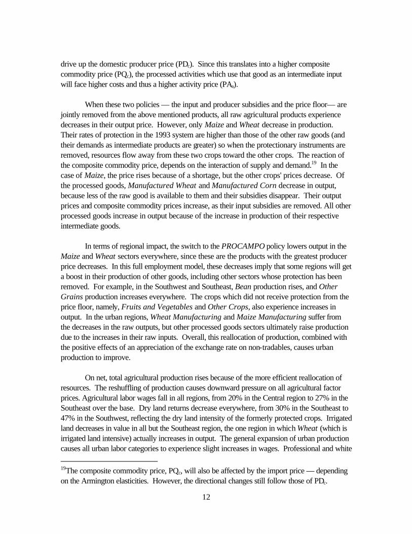
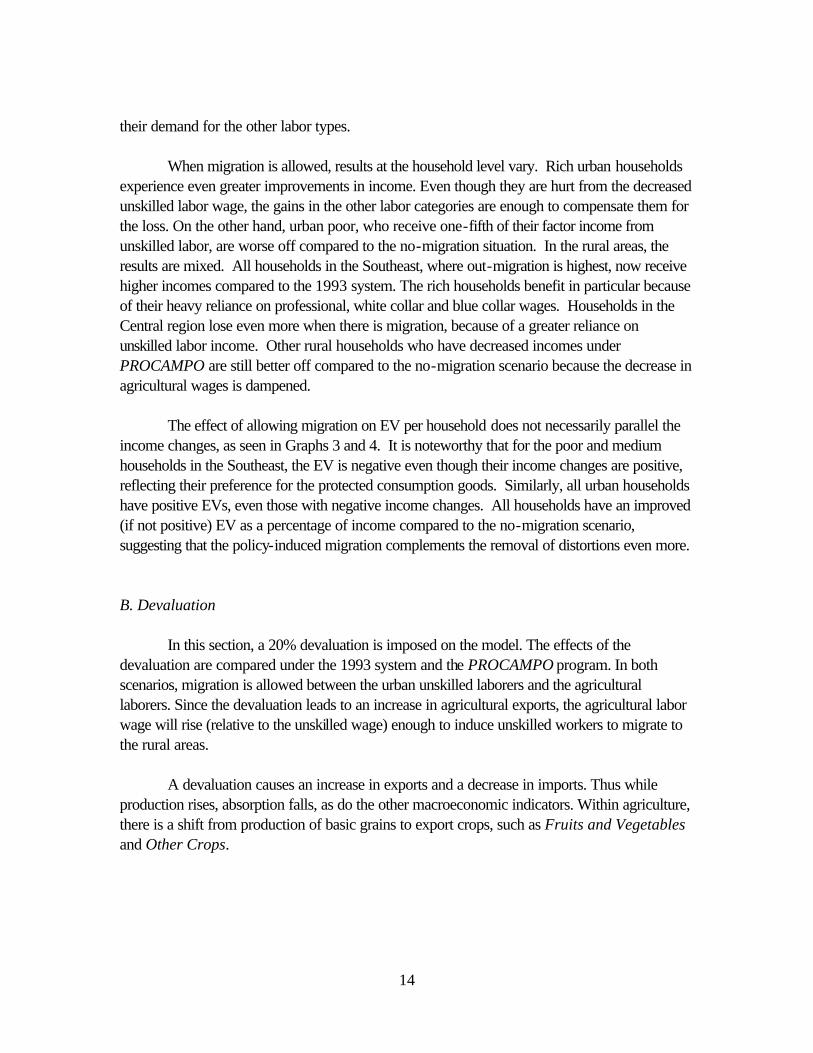
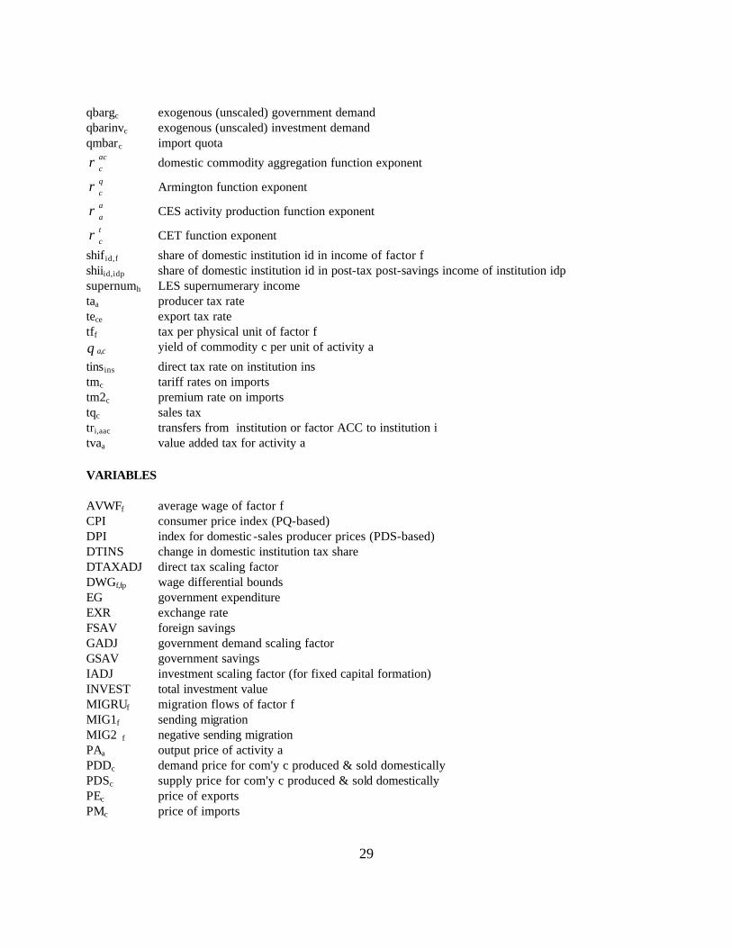
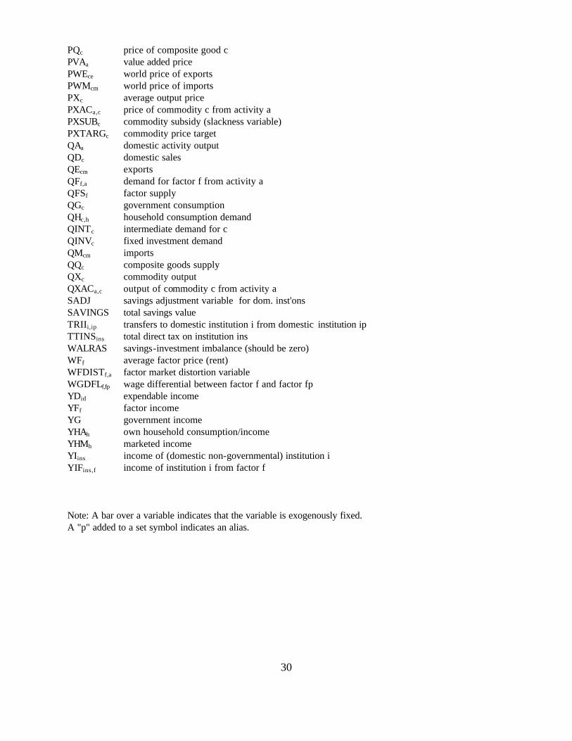
collar wages benefit the most, with raises above one and a half percent each. Graphs 1 and 2 show the income changes and equivalent variation measures for

households following the policy change. All rural households get lower incomes when the 1993 system is removed and the PROCAMPO policy is implemented. They suffer from the decreased land and labor returns, with the rich North households losing the greatest amount nationally, of more than 22% over the base. The other rural dwellers also lose, though those who rely more on urban factor income (for example, the rich in the Southeast) see almost no change in income. In the urban area, where all labor returns increase, all households gain slightly, from a 0.2% increase in income for the poor and up to 1.1% increase for the rich. In welfare terms, most rural households see a decline. The rural rich in the North see the biggest decrease in equivalent variation (EV) as a percentage of their income, almost 2%. However, the rural rich of the Southeast experience an increase in EV, suggesting that although their incomes are falling, they are better off from an efficiency point of view. This is not surprising given that in the base they consume very little of the protected goods. All urbanites have a positive EV. Overall, the sum of EV across households is positive, reflecting the move from a distorting to a relatively non-distorting system. 2. Migration

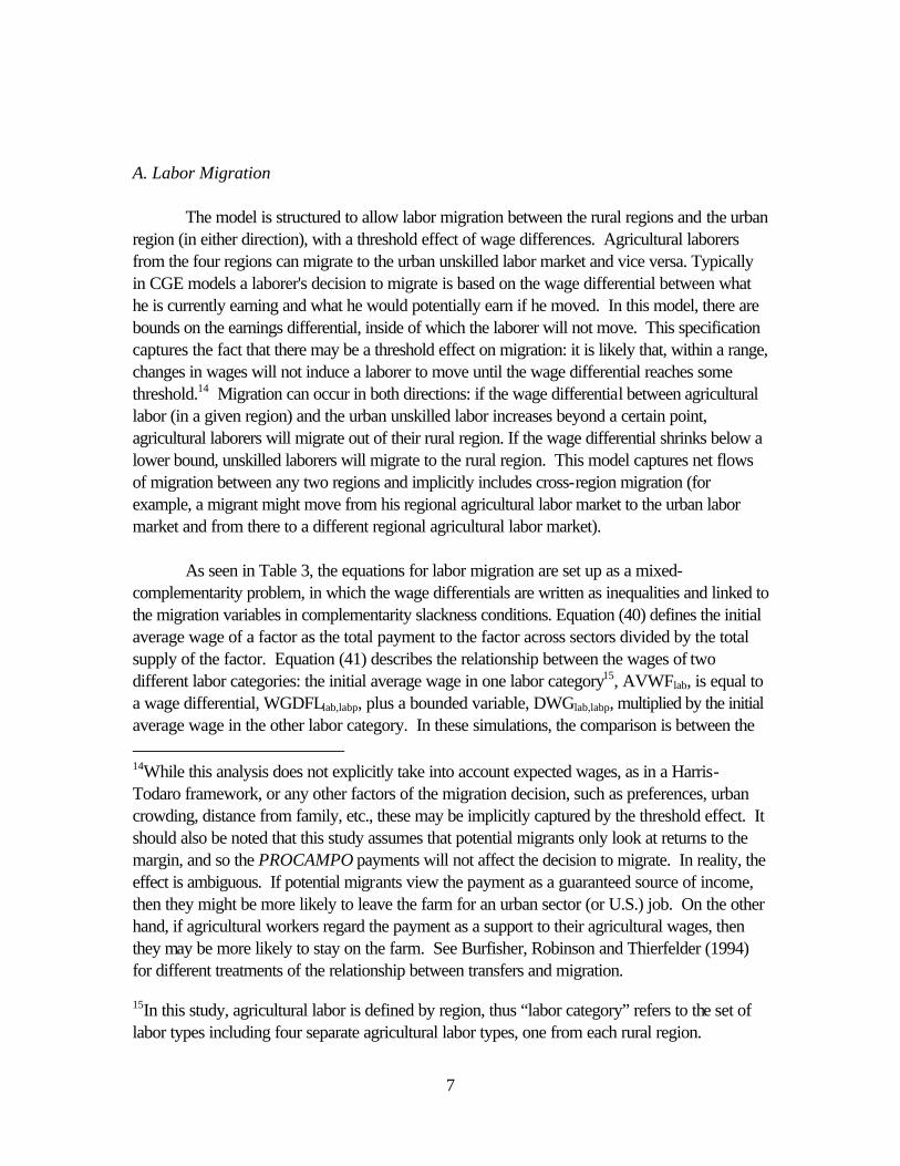
When the PROCAMPO system is simulated and migration is allowed, the economy expands by even more. The policy lowers agricultural labor wages in all four regions, thus stimulating migration to the urban unskilled labor sector. 820 thousand laborers migrate to the urban sector, with almost 420 thousand leaving agriculture in the Southeast and 250 thousand from the Southwest. The increase of almost 14% of the unskilled labor force (and about 3.5% of the total urban labor force) due to migration causes a greater expansion of urban output. Real GDP and absorption each rise by over 2 ½ %.

The consequences at the micro level are positive in most respects, compared to the

situation of no migration. The influx of agricultural laborers into urban activities cushions the fall in the agricultural wage that occurs in the situation of no migration, but the change is still negative: agricultural wages fall over the base case by nearly 11%.20 All land types in all regions experience a greater decrease in their returns compared to the no-migration scenario. This is because there are now fewer workers per land area. In the urban area, the unskilled labor wage decreases because there is now a bigger supply of workers following the in-migration. Whereas the unskilled labor return rose without migration, it now falls by about 10%. All other labor types experience slightly greater increases than when there was no migration. This is because with more unskilled labor, all productive sectors see an increase in output, which then increases

20Note that by construction, when migration is in place, wages are constrained to

change by the same amount for all receiving factors (ie., in Equations 41-43, DWGlab,labp has the same bounds — in percentage terms — for all factors).

14

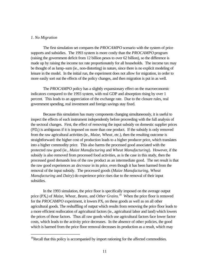
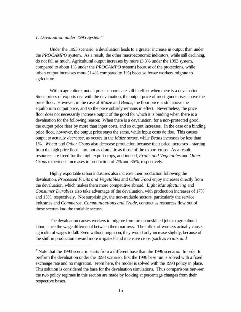
their demand for the other labor types. When migration is allowed, results at the household level vary. Rich urban households

experience even greater improvements in income. Even though they are hurt from the decreased unskilled labor wage, the gains in the other labor categories are enough to compensate them for the loss. On the other hand, urban poor, who receive one-fifth of their factor income from unskilled labor, are worse off compared to the no-migration situation. In the rural areas, the results are mixed. All households in the Southeast, where out-migration is highest, now receive higher incomes compared to the 1993 system. The rich households benefit in particular because of their heavy reliance on professional, white collar and blue collar wages. Households in the Central region lose even more when there is migration, because of a greater reliance on unskilled labor income. Other rural households who have decreased incomes under PROCAMPO are still better off compared to the no-migration scenario because the decrease in agricultural wages is dampened.

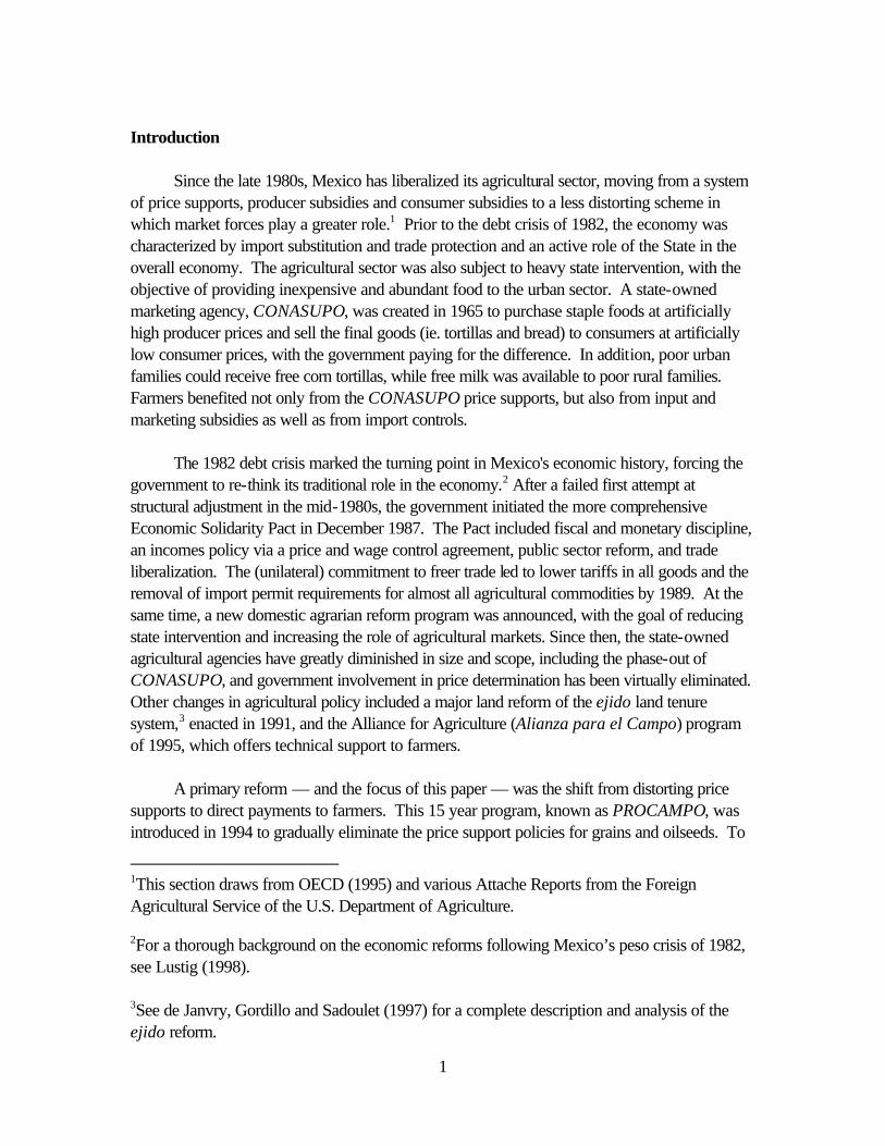
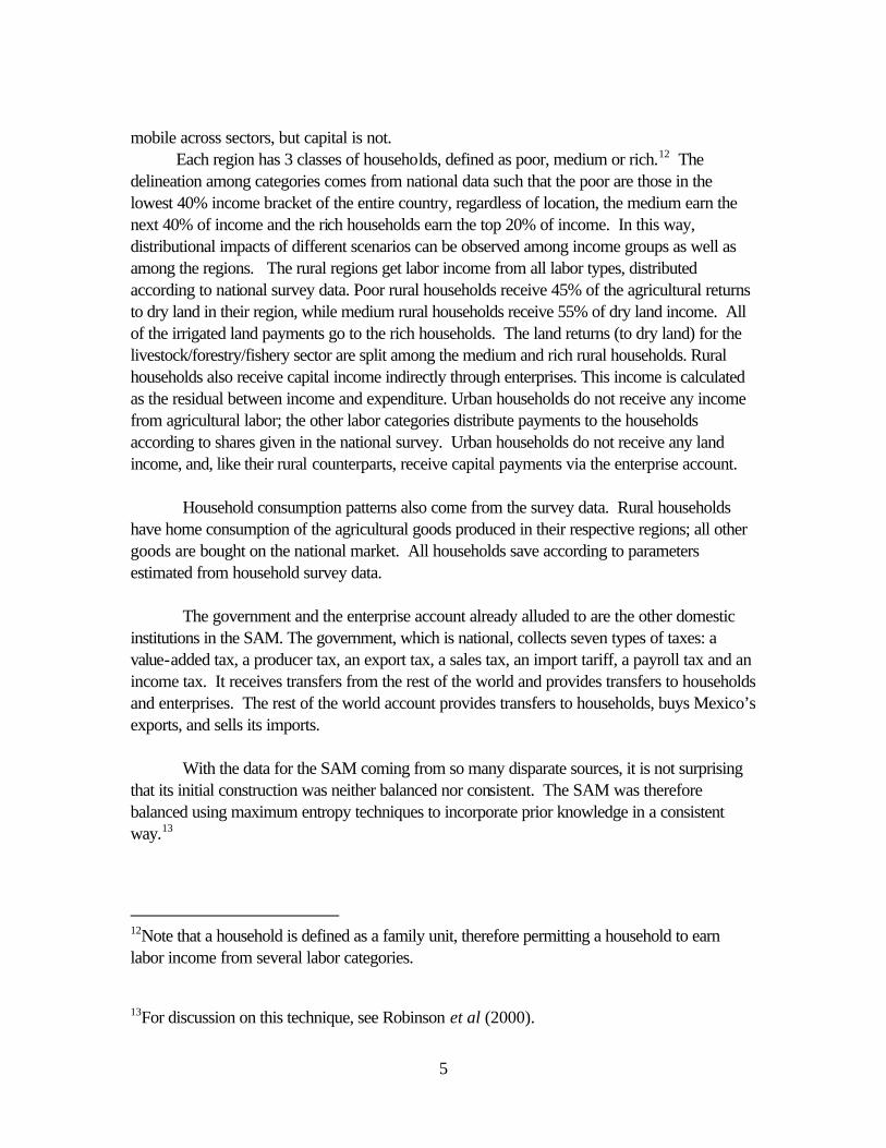
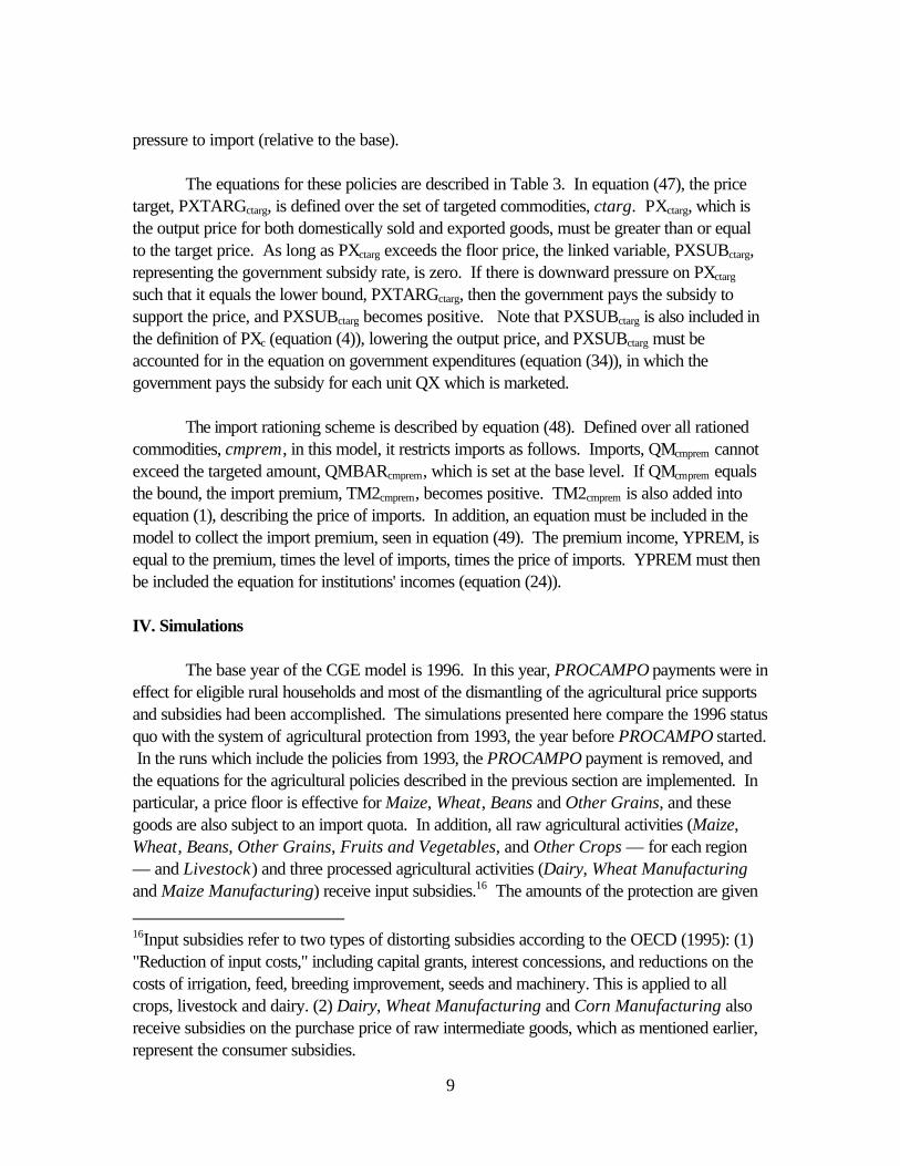
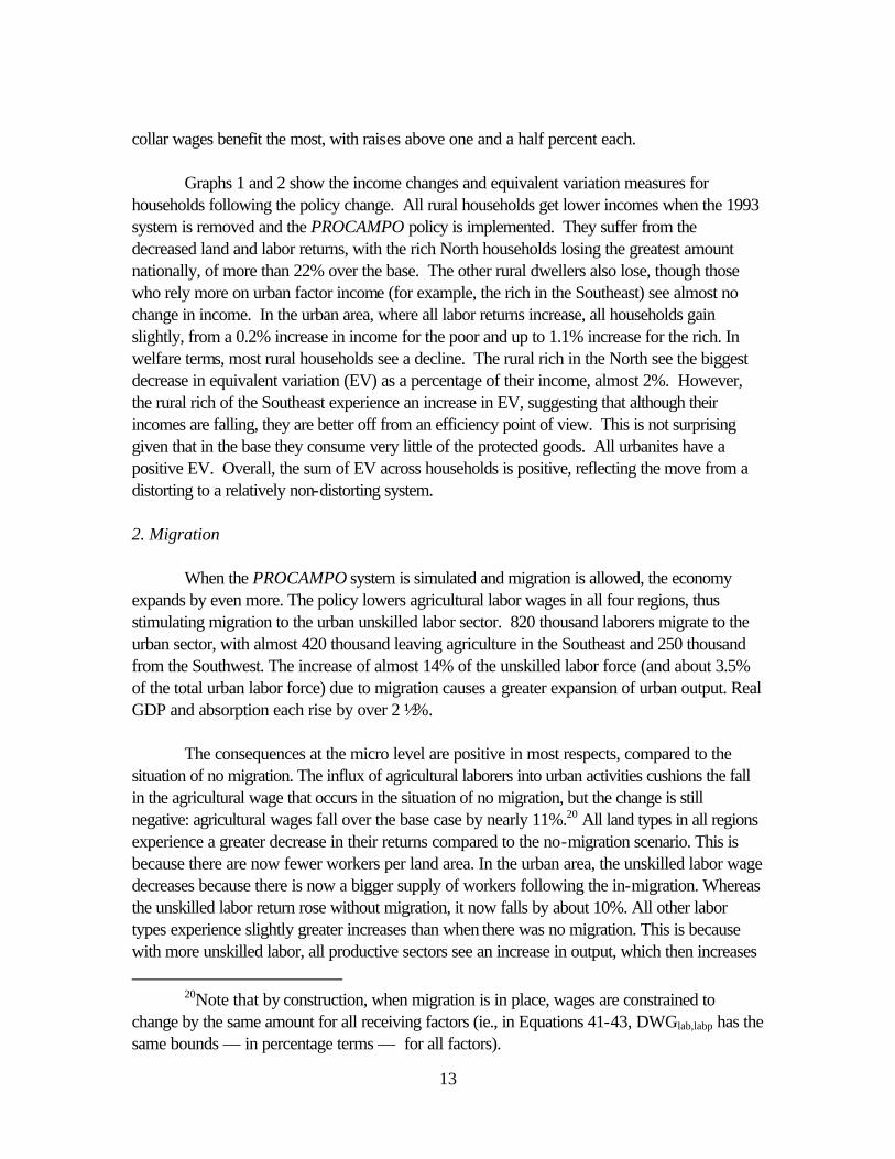
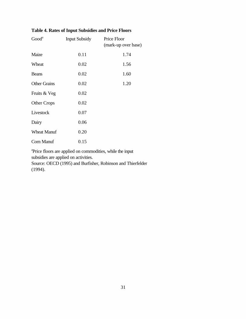
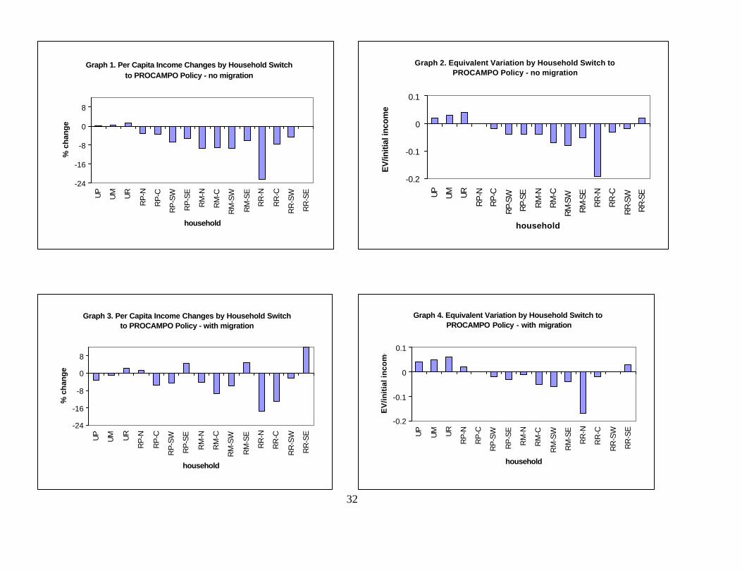
The effect of allowing migration on EV per household does not necessarily parallel the

income changes, as seen in Graphs 3 and 4. It is noteworthy that for the poor and medium households in the Southeast, the EV is negative even though their income changes are positive, reflecting their preference for the protected consumption goods. Similarly, all urban households have positive EVs, even those with negative income changes. All households have an improved (if not positive) EV as a percentage of income compared to the no-migration scenario, suggesting that the policy-induced migration complements the removal of distortions even more. B. Devaluation

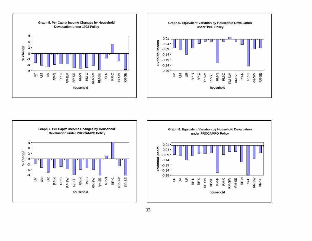
In this section, a 20% devaluation is imposed on the model. The effects of the devaluation are compared under the 1993 system and the PROCAMPO program. In both scenarios, migration is allowed between the urban unskilled laborers and the agricultural laborers. Since the devaluation leads to an increase in agricultural exports, the agricultural labor wage will rise (relative to the unskilled wage) enough to induce unskilled workers to migrate to the rural areas.

A devaluation causes an increase in exports and a decrease in imports. Thus while

production rises, absorption falls, as do the other macroeconomic indicators. Within agriculture, there is a shift from production of basic grains to export crops, such as Fruits and Vegetables and Other Crops.

15

1. Devaluation under 1993 System21 Under the 1993 scenario, a devaluation leads to a greater increase in output than under

the PROCAMPO system. As a result, the other macroeconomic indicators, while still declining, do not fall as much. Agricultural output increases by more (3.3% under the 1993 system, compared to about 1% under the PROCAMPO system) because of the protections, while urban output increases more (1.4% compared to 1%) because fewer workers migrate to agriculture.

Within agriculture, not all price supports are still in effect when there is a devaluation.

Since prices of exports rise with the devaluation, the output price of most goods rises above the price floor. However, in the case of Maize and Beans, the floor price is still above the equilibrium output price, and so the price subsidy remains in effect. Nevertheless, the price floor does not necessarily increase output of the good for which it is binding when there is a devaluation for the following reason: When there is a devaluation, for a non-protected good, the output price rises by more than input costs, and so output increases. In the case of a binding price floor, however, the output price stays the same, while input costs do rise. This causes output to actually decrease, as occurs in the Maize sector, while Beans increases by less than 1%. Wheat and Other Crops also decrease production because their price increases – starting from the high price floor – are not as dramatic as those of the export crops. As a result, resources are freed for the high export crops, and indeed, Fruits and Vegetables and Other Crops experience increases in production of 7% and 36%, respectively.

Highly exportable urban industries also increase their production following the

devaluation. Processed Fruits and Vegetables and Other Food enjoy increases directly from the devaluation, which makes them more competitive abroad. Light Manufacturing and Consumer Durables also take advantage of the devaluation, with production increases of 17% and 15%, respectively. Not surprisingly, the non-tradable sectors, particularly the service industries and Commerce, Communications and Trade, contract as resources flow out of these sectors into the tradable sectors.

The devaluation causes workers to migrate from urban unskilled jobs to agricultural

labor, since the wage differential between them narrows. The influx of workers actually causes agricultural wages to fall. Even without migration, they would only increase slightly, because of the shift in production toward more irrigated-land intensive crops (such as Fruits and

21Note that the 1993 scenario starts from a different base than the 1996 scenario. In order to perform the devaluation under the 1993 scenario, first the 1996 base run is solved with a fixed exchange rate and no migration. From here, the model is solved with the 1993 policy in place. This solution is considered the base for the devaluation simulations. Thus comparisons between the two policy regimes in this section are made by looking at percentage changes from their respective bases.

16

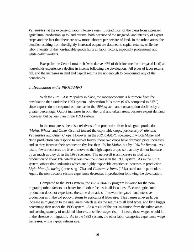
Vegetables) at the expense of labor intensive ones. Instead most of the gains from increased agricultural production go to land returns, both because of the irrigated-land intensity of export crops and the fact that there are now more laborers per hectare of land. In the urban areas, the benefits resulting from the slightly increased output are destined to capital returns, while the labor intensity of the non-tradable goods hurts all labor factors, especially professional and white collar workers.

Except for the Central rural rich (who derive 40% of their income from irrigated land) all

households experience a decline in income following the devaluation. All types of labor returns fall, and the increases in land and capital returns are not enough to compensate any of the households.

2. Devaluation under PROCAMPO

With the PROCAMPO policy in place, the macroeconomy is hurt more from the

devaluation than under the 1993 system. Absorption falls more (9.4% compared to 8.5%) since exports do not respond as much as in the 1993 system and consumption declines by a greater percentage. Output increases in both the rural and urban areas, because export demand increases, but by less than in the 1993 system.

In the rural areas, there is a relative shift in production from basic grain production

(Maize, Wheat, and Other Grains) toward the exportable crops, particularly Fruits and Vegetables and Other Crops. However, in the PROCAMPO scenario, in which Maize and Bean production can respond to market forces, these two crops have dramatic price increases, and so they increase their production (by less than 1% for Maize, but by 19% for Beans). As a result, fewer resources are free to move to the high export crops, so that they do not increase by as much as they do in the 1993 scenario. The net result is an increase in total rural production of about 1%, which is less than the increase in the 1993 system. As in the 1993 system, other urban industries which are highly exportable experience increases in production. Light Manufacturing (increasing 17%) and Consumer Items (15%) stand out in particular. Again, the non-tradable sectors experience decreases in production following the devaluation.

Compared to the 1993 system, the PROCAMPO program is worse for the non-

migrating urban factors but better for all other factors in all locations. Because agricultural production does not experience the same dramatic shift toward irrigated-land intensive production as in the old policy, returns to agricultural labor rise. This causes an even larger increase in migration to the rural areas, which raises the returns to all land types, and by a bigger percentage than under the 1993 system. As a result of the out-migration from the urban areas and ensuing scarcity of unskilled laborers, unskilled wages rise -- indeed, these wages would fall in the absence of migration. As in the 1993 system, the other labor categories experience wage decreases, while capital returns rise.

17

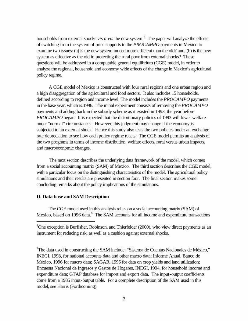
Graph 7 shows that most households are worse off following the devaluation. The Rich households in the North and Central areas are the exceptions, gaining from the increased land returns. The other rural households still lose income because, although they receive higher returns to agricultural labor and land, they rely more heavily on urban-based factors for their income. Compared to the 1993 system, however, many of the rural households lose less income, particularly those who rely heavily on unskilled wages. The urban households also experience income losses from the evaluation, but the decrease is lower for the poor and medium households under PROCAMPO. Urban rich, who do not benefit as much from unskilled wages, experience a slightly larger decline in their incomes under PROCAMPO.

These changes in factor income do not tell the whole story, since the effects of

consumption possibilities are not taken into account. A comparison of the ratios of EV to base income by household associated with the two policy regimes (Graphs 6 and 8) shows that in fact, the urban households see very little change in welfare, while most rural households actually fare better under the 1993 system. This is due to the protectionist policies which help cushion the drop in income for rural consumers. VI. Conclusions

This paper uses a CGE model to compare the 1993 system of agricultural supports to

the less distorting 1996 system. In the absence of exogenous shocks, the newer system is better for the economy. All macroeconomic indicators increase, and even the agricultural sector experiences increases in output. Because of the strong linkages between rural production and urban production, the urban sector also benefits from the policy. Although the 1993 system should protect the rural households, because they are so dependent on urban sector wages for income, some are ultimately better off when the new policy is implemented.

When the economy is subjected to a negative external shock, the prognosis is not so

clear. The exchange rate shock simulated in this study negates the inefficiencies of the 1993 system, by funneling resources from the protected crops toward the export crops. Although the macroeconomy is generally better off with the 1993 system following the shock, urban households may be worse off. Given their size in the overall population, reverting to the protectionist 1993 system would be politically and socially infeasible.

Nevertheless, as the 1994 currency crisis in Mexico showed, some government

intervention is needed to provide a safety net for the most economically vulnerable groups, particularly in the countryside. With that in mind, the Mexican government announced a new anti-poverty program, PROGRESA (Program of Health, Education and Nutrition) in 1997. The program is essentially a conditional cash-transfer program whereby households receive money if they enroll their children in school and ensure adequate attendance and/or if family members adhere to a pre-determined schedule of visits to health centers. Not only is this kind of program less distorting for the economy as a whole, and to the rural population in particular, it also has a

18

built-in “human capital” component which may help break the cycle of poverty. The simulations highlight several features of the model. First, it is obvious that a national

shock can have different implications for different regions of the economy. The exchange rate devaluation impacts the entire economy, but those who can take advantage of increased export capability, such as the rural Central households, are not as adversely affected. The model also underscores the wide diversity of income sources of rural households. While this may help cushion their incomes during times of agricultural downturns, the heavy reliance on off-farm income implies that they have a vested interest in the performance of the urban economy.

Finally, any judgment on the distributive effects of the either program must include the

caveat that the disaggregation of the SAM is not enough, and may be hiding what is happening at the lowest end of the income spectrum. It may be that the very poorest agricultural households rely much more on rural labor and less on urban factor income. This would suggest that they would benefit from policies that protect the crops on which they depend the most for their income (as well as consumption). Such a system would have to ensure that those without high participation in the market economy would be able to take advantage of its assistance.

19

References Banco de Mexico. 1996. Informe Anual (Mexico City). Burfisher, Mary, Sherman Robinson and Karen Thierfelder. 2000. “North American Farm Programs and the WTO,” American Journal of Agricultural Economics 82(3). Burfisher, Mary, Sherman Robinson and Karen Thierfelder. 1994. "NAFTA, Mexican Agricultural Policy Reform, and Labor Mobility," in Thomas Grennes and Gary Williams, eds. NAFTA and Agriculture: Will the Experiment Work? Minneapolis: International Agricultural Trade Research Consortium. de Janvry, Alain, Elisabeth Sadoulet, and Gustavo Gordillo. 1995. “NAFTA and Mexico’s Maize Producers,” World Development 23(8). de Janvry, Alain, Gustavo Gordillo, and Elisabeth Sadoulet. 1997. Mexico’s Second Agrarian Reform (Center for U.S.- Mexican Studies at the University of California, San Diego). Harris, Rebecca Lee. Forthcoming. Estimation of a Regionalized Mexican Social Accounting Matrix: Using Entropy Techniques to Reconcile Disparate Data Sources. Proceedings from the Seminario Internacional Insumo-Producto: Regional y Otras Aplicaciones (International Input-Output Seminar: Regional and Other Applications) in Guadalajara, Mexico, September 2-4, 1999. Instituto Nacional de Estadística, Geografía, e Informática (INEGI). 1998. Sistema de Cuentas Nacionales de México. Instituto Nacional de Estadística, Geografía, e Informática (INEGI). 1994. Encuesta Nacional de Ingresos y Gastos de los Hogares. Josling, Tim. 1992. “NAFTA and Agriculture: A Review of the Economic Impacts,” in Lustig, Bosworth and Lawrence, ed., North American Free Trade: Assessing the Impact (Washington, DC: The Brookings Institution Press). Levy, Santiago and Sweder van Wijnbergen. 1992. “Mexican Agriculture in the Free Trade Agreement: Transition Problems in Economic Reform,” OECD Development Centre Technical Papers: No. 63. Lustig, Nora. 1998. Mexico: The Remaking of an Economy, 2nd Edition (Washington, DC: Brookings Institution Press) Lustig, Nora, Barry P. Bosworth and Robert Z. Lawrence, ed. 1992. North American Free

20

Trade: Assessing the Impact (Washington, DC: The Brookings Institution Press). Organisation for Economic Development and Co-operation (OECD). 1995. Review of Agricultural Policies in Mexico. Pyatt, Graham and Jeffery Round, eds. 1985. Social Accounting Matrices. A Basis for Planning. Washington, DC: The World Bank. Robinson, Sherman, Andrea Cattaneo and Moataz El-Said. 2000. “Updating and Estimating a Social Accounting Matrix Using Entropy Methods.” International Food Policy Research Institute, Trade and Macroeconomics Division, Discussion Paper No. 58. Sadoulet, Elisabeth, Alain de Janvry, and Benjamin Davis. 1999. “Cash Transfer Programs with Income Multipliers: PROCAMPO in Mexico.” (Draft Manuscript) Secretaría de Agricultura, Ganadería y Desarrollo Rural (SAGAR). 1996. Anuario Estadístico de la Producción Agrícola de los Estados Unidos Mexicanos, Vols. I and II.

21

Table 1. Regions in CGE Model 1. North

-Baja California Norte -Baja California Sur -Sonora -Sinaloa -Chihuahua -Coahuila -Nuevo Leon

2. Central

-Durango -Zacatecas -Aguascalientes -San Luis Potosi -Guanajuato -Queretaro -Hidalgo -Tlaxcala -Puebla -Tamaulipas

3. Southwest -Nayarit -Jalisco -Colima -Michoacan -Estado de Mexico -Distrito Federal -Guerrero -Morelos

4. Southeast

-Veracruz -Oaxaca -Chiapas -Tabasco -Campeche -Yucatan -Quintana Roo

22

Table 2. National Sectors in Model

1. Maize 2. Wheat 3. Beans 4. Other Grains (Sorghum, Barley) 5. Fruits and Vegetables 6. Other Crops (Tobacco, Hemp, Cotton, Cocoa, Sugar, Coffee, Soy, Safflower, Sesame and

Others) 7. Livestock/Forestry/Fisheries (Bovines, Goats, Sheep, Bees, Poultry and Others, Forestry and

Fisheries) 8. Dairy 9. Prepared Fruits and Vegetables 10. Wheat Manufacturing 11. Corn Manufacturing 12. Sugar Manufacturing 13. Other Processed Foods (Coffee Manufacturing, Processed Meats, Oils and Fats, Feeds, Alcohol,

Beverages and Others) 14. Light Manufacturing (Lumber, Wood, Paper, Print, and Cigar Manufacturing, Soft Fiber Textiles,

Hard Fiber Textiles, Other Textiles, Leather, Apparel) 15. Intermediates (Chemicals, Synthetics, Rubber, Glass, Cement,Fertilizers, Other Chemicals, Oil

Refining, Oil and Gasoline, Petrochemicals, Coal, Iron, Non-Ferrous Metal, Sand/Gravel, Minerals)

16. Consumer Items (Pharmeceuticals, Soaps, Plastic, Metal Furnishings, Household Appliances, Electronic Equipment, Automobiles and Parts)

17. Capital Goods (Metal Products, Metal Manufacturing, Non-Electronic Machines, Electronic Machines, Other Electric Goods, Transportation Materials, Mineral Manufacturing, Iron Manufacturing, Non-Ferrous Metal Manufacturing, Others)

18. Professional Services (Professional Services, Education, Medical, Finance/Real Estate, Public Administration and Defense, Electricity, Gas and Water)

19. Other Services (Other Services, Restaurants 20. Construction 21. Commerce, Trade and Transportation

23

Table 3. Equations of CGE Model (A listing of the sets, variables and parameters follows this table) PRICE BLOCK

(1) ( )2cmcm cm cmPM = 1+tm TM EXR PWM ⋅ + ⋅

(2) ( )ce ce cePE =PWE 1-te EXR ⋅ ⋅

(3) c cmc c c c cm(1- ) = PDD + PMPQ tq QQ QD QM⋅ ⋅ ⋅ ⋅

(4) ( ) ( )1c cd ce cc cd cePX = PDS + PE PXSUBQX QD QE⋅ ⋅ ⋅ ⋅ −

(5) c cPDD = PDS

(6) , ,a a c a cc

PA = PXACθ ⋅∑

(7) ( )1a a a a ca cc

PVA PA ta insub ica PQ= − + − ⋅∑

(8) ccc

CPI = cwts PQ⋅∑

(9) cd cdcd

DPI = dwts PDS⋅∑

SUPPLY AND TRADE BLOCK

(10)

1

, ,

aa aaa a

a f a f aaf

= QFQAρ

ρα δ−

− ⋅

∑

(11) 1, , , ,

aa aa

aa

1- -1

-a a afp,af f a a a a f p a f a f a

fp

WF WFDIST = PVA (1-tva ) QF QFρ

ρρα δ δ − − ⋅ ⋅ ⋅ ⋅ ⋅ ⋅ ⋅

∑

(12) , ac aca

= icaQINT QA⋅∑

24

Table 3, continued

(13) , , ( )a,ha c a c ah

QXAC = - QA QAHθ ⋅ ∑

(14),( )ac acc cd

1-ac -ac

cd cd a c d a,cda

QX = QXAC ρ ρα δ⋅ ⋅∑

(15)1

1

, ,( ) acac ac ccc - -1-ac ac acca,c ap,cc a p c a p c ap,c

ap

= QXAC QXACPXAC PX ρ ρρα δ δ− −

⋅ ⋅ ⋅ ⋅⋅∑

(16)1

[ ]t t tce ce cet t tce ce cece ce ce = + (1- )QX QE QD ρρ ρα δ δ

−

⋅ ⋅ ⋅

(17)& &cen cd cen cd = QX QD

(18)

1

1tce

tce ce

ce ce tce ce

1 - PE = QE QDPDS

ρδδ

−− ⋅ ⋅

(19) & &&& & && & &

[ ]q q

qcm cd cm cdcm cd

1-- -q q qcm cd cm cd cm cdcm cd cm cd cm cd = + (1- )QQ QM QDρ ρ ρα δ δ⋅ ⋅ ⋅

(20) cnnorcdn cnnorcdn = QQ QD

(21)&

& && &

& &

qcm cd

1q 1+

cm cd cm cdcm cd cm cd q

cm cd cm cd

PDD = QM QD1 - PM

ρδδ

⋅ ⋅

INSTITUTION BLOCK

(22) , f,af f f aa

YF = WF WFDIST QF⋅ ⋅∑

(23) [ ] ( )id, f row,ff fid, f = YF - EXR 1 tfshif trYIF ⋅ ⋅ ⋅ −

(24) , , id,gov id,rowid id f id idp cmprem cmpremid cmpremf

YI = YIF + TRII + + EXR shprem YPREMtr tr ⋅ + ⋅∑ ∑∑

(25) ( )1 01id id idTTINS = DTAXADJ tins + DTINS p⋅ ⋅ ⋅

25

Table 3, continued.

(26) , ,i d e n id en en enenTRII = shii (1-SADJ ) (1-TTINS ) YImps⋅ ⋅ ⋅ ⋅

(27) , , [( ) ( ) ]i d h i d h h h hhTRII = shii 1-SADJ 1-TTINS YHM YHAmps⋅ ⋅ ⋅ ⋅ +

(28) ,1 1 1( ) ( ) ( )h i n s h h h hhins

YD = -SADJ - shii TTINS YHM YHAmps + ⋅ ⋅ ⋅ − ⋅

∑

(29) , , , , )(m m m hac h c h cp c p h a hc c,h c h

cp a

= + PQPQ QH PQ YD PAγ β γ γ⋅ ⋅ ⋅ − ⋅ − ⋅∑ ∑

(30) , , , ,( )h h m hha a a h a h c c h ap a p ha,h

c ap

PA = PA + PQ PAQAH YDγ β γ γ⋅ ⋅ ⋅ − ⋅ − ⋅∑ ∑

(31) a,hh aa

YHA = PA QAH⋅∑

(32) h h hYHM YI YHA= −

(33)

,

( )

( )

id id a a aid a

a a a cm cm cma cm

ce ce cece

f f c c c govrowf c

YG TTINS YI tva PVA QA

ta PA QA tm QM PWM EXR

te QE PWE EXR

YF tf tq PQ QQ tr EXR

= ⋅ + ⋅ ⋅

+ ⋅ ⋅ + ⋅ ⋅ ⋅

+ ⋅ ⋅ ⋅

+ ⋅ + ⋅ ⋅ + ⋅

∑ ∑

∑ ∑

∑∑ ∑

(34) id,gov c insc c ac id a c ins

EG = PQ QG insubtr PXSUB PROCAMPO+⋅ + + +∑ ∑ ∑ ∑ ∑

(35) c c = GADJQG qg⋅

(36)GSAV = YG-EG

(37) c c = IADJQINV qinv⋅

(38) c ccc

INVEST = PQ QINV qdst( + )⋅∑

26

Table 3, continued.

(39)

( )

[( ) ]

en enenen

h h hhh

SAVINGS = SADJ 1-TTINS YI mps

+ SADJ 1-TTINS YHM +YHA + GSAV + FSAV EXRmps

⋅ ⋅ ⋅

⋅ ⋅ ⋅ ⋅

∑

∑

LABOR MIGRATION EQUATIONS

(40), ,

,

f a f f aa

ff ap

ap

WFDIST wf QFAVWF

QF

⋅ ⋅=

∑∑

(41) ( ), ,1lab lablabp lablabp labpAVWF WGDFL DWG AVWF = ⋅ + ⋅

(42) , 0.01,

1 0smigrmigDWG

MIG

≤

≤

(43) , 0.01,

1 0smigrmigDWG

MIG

≥

≥

(44) ( ), ,1 2smig smig rmig smig rmigrmig

MIGRU MIG MIG= − −∑

(45) 0lab lab labQFS QFS MIGRU= +

(46) 0lablab

MIGRU =∑

AGRICULTURAL POLICY

(47),

0ctarg ctarg

ctarg

PXTARG PX

PXSUB

≤

≥

(48),

2 0cmprem cmprem

cmprem

QMBAR QM

TM

≥

≥

27

Table 3, continued. SYSTEM CONSTRAINT BLOCK AND DEFINITIONS OF MACROECONOMIC AGGREGATES

(49) c,h c c cc ch

= + QQ QINT QH QG QINV qdst + + + ∑

(50) ,f afa

= QFQFS ∑

(51) , ins,rowcm row f cecm cecm f ce ins

PWM + tr PWE + FSAVQM QE tr = +⋅ ⋅∑ ∑ ∑ ∑

(52) SAVINGS = INVEST + WALRAS

(53)TGDP = TCON + INVEST + TGOV + TEXP - TIMP

(54) c,h a,hc ac,h a,h

TCON = PQ PAQH QAH+⋅ ⋅∑ ∑

(55) ce cece

TEXP EXR PWEQE= ⋅ ⋅∑

(56) cm cmcm

TIMP QM EXR PWM= ⋅ ⋅∑

(57) c cc

TGOV = PQ QG ⋅∑

(58)TABS = TGDP + TIMP - TEXP

(59) INVEST = INVSHR TABS⋅

(60)TGOV = GOVSHR TABS⋅

28

Table 3a. Sets, Variables and Parameters of the CGE Model. SETS AAC global set (SUBSETS OF AAC) a Activities c Commodities cm(c) Imported Commodities cnm(c) Non-imported Commodities ce(c) Exported Commodities cne(c) Non-exported Commodities f Factors lab(f) Labor Factors ld(f) Land Factors ins Institutions (domestic and rest of world) id(ins) Domestic Institutions h(ins) Households en(ins) Enterprises PARAMETERS

aaα shift parameter for CES activity production function acaα shift parameter for domestic commodity aggregation fn qcα shift parameter for Armington function tcα shift parameter for CET function ha,hβ LES marginal budget shares for home consumed goods (activities) mc,hβ LES marginal budget shares for marketed goods (commodities)

cwtsc consumer price index weights af,aδ share parameter for CES activity production function aca,cδ share parameter for domestic commodity aggregation fn qcδ share parameter for Armington function tcδ share parameter for CET function

dwtsc domestic sales price weights ha,hγ LES subsistence minima for home consumed goods (activities) mc,hγ LES subsistence minima for marketed goods (commodities)

icac,a intermediate input c per unit of activity a mps ins marginal propensity to save for domestic institution p01ins 0-1 parameter (1 for institution with variable tax rate -0 for others) procampoins PROCAMPO payment qbardstc inventory investment by sector of origin

29

qbargc exogenous (unscaled) government demand qbarinvc exogenous (unscaled) investment demand qmbarc import quota

accρ domestic commodity aggregation function exponent qcρ Armington function exponent aaρ CES activity production function exponent tcρ CET function exponent

shifid,f share of domestic institution id in income of factor f shiiid,idp share of domestic institution id in post-tax post-savings income of institution idp supernumh LES supernumerary income taa producer tax rate tece export tax rate tff tax per physical unit of factor f

a,cθ yield of commodity c per unit of activity a

tinsins direct tax rate on institution ins tmc tariff rates on imports tm2c premium rate on imports tqc sales tax tri,aac transfers from institution or factor ACC to institution i tvaa value added tax for activity a VARIABLES AVWFf average wage of factor f CPI consumer price index (PQ-based) DPI index for domestic -sales producer prices (PDS-based) DTINS change in domestic institution tax share DTAXADJ direct tax scaling factor DWGf,fp wage differential bounds EG government expenditure EXR exchange rate FSAV foreign savings GADJ government demand scaling factor GSAV government savings IADJ investment scaling factor (for fixed capital formation) INVEST total investment value MIGRUf migration flows of factor f MIG1f sending migration MIG2 f negative sending migration PAa output price of activity a PDDc demand price for com'y c produced & sold domestically PDSc supply price for com'y c produced & sold domestically PEc price of exports PMc price of imports

30

PQc price of composite good c PVAa value added price PWEce world price of exports PWMcm world price of imports PXc average output price PXACa,c price of commodity c from activity a PXSUBc commodity subsidy (slackness variable) PXTARGc commodity price target QAa domestic activity output QDc domestic sales QEcm exports QFf,a demand for factor f from activity a QFSf factor supply QGc government consumption QHc,h household consumption demand QINTc intermediate demand for c QINVc fixed investment demand QMcm imports QQc composite goods supply QXc commodity output QXACa,c output of commodity c from activity a SADJ savings adjustment variable for dom. inst'ons SAVINGS total savings value TRIIi,ip transfers to domestic institution i from domestic institution ip TTINSins total direct tax on institution ins WALRAS savings-investment imbalance (should be zero) WFf average factor price (rent) WFDISTf,a factor market distortion variable WGDFLf,fp wage differential between factor f and factor fp YDid expendable income YFf factor income YG government income YHAh own household consumption/income YHMh marketed income YIins income of (domestic non-governmental) institution i YIFins,f income of institution i from factor f

Note: A bar over a variable indicates that the variable is exogenously fixed. A "p" added to a set symbol indicates an alias.

31

Table 4. Rates of Input Subsidies and Price Floors Gooda

Input Subsidy

Price Floor (mark-up over base)

Maize

0.11

1.74

Wheat

0.02

1.56

Beans

0.02

1.60

Other Grains

0.02

1.20

Fruits & Veg

0.02

Other Crops

0.02

Livestock

0.07

Dairy

0.06

Wheat Manuf

0.20

Corn Manuf

0.15

aPrice floors are applied on commodities, while the input subsidies are applied on activities. Source: OECD (1995) and Burfisher, Robinson and Thierfelder (1994).

32

Graph 1. Per Capita Income Changes by Household Switch to PROCAMPO Policy - no migration

-24

-16

-8

0

8UP UM UR

RP-

N

RP-

C

RP-

SW

RP-

SE

RM

-N

RM

-C

RM

-SW

RM

-SE

RR

-N

RR

-C

RR

-SW

RR

-SE

household

% c

hang

e

Graph 4. Equivalent Variation by Household Switch to PROCAMPO Policy - with migration

-0.2

-0.1

0

0.1

UP UM UR

RP-

N

RP-

C

RP-

SW

RP-

SE

RM

-N

RM

-C

RM

-SW

RM

-SE

RR

-N

RR

-C

RR

-SW

RR

-SE

household

EV

/initi

al in

com

e

Graph 2. Equivalent Variation by Household Switch to PROCAMPO Policy - no migration

-0.2

-0.1

0

0.1

UP UM UR

RP-

N

RP-

C

RP-S

W

RP-S

E

RM

-N

RM

-C

RM-S

W

RM-S

E

RR

-N

RR

-C

RR-S

W

RR-S

E

household

EV

/initi

al in

com

e

Graph 3. Per Capita Income Changes by Household Switch to PROCAMPO Policy - with migration

-24

-16

-8

0

8

UP UM UR

RP-

N

RP-

C

RP-

SW

RP-

SE

RM

-N

RM

-C

RM

-SW

RM

-SE

RR

-N

RR

-C

RR

-SW

RR

-SE

household

% c

hang

e

33

Graph 5. Per Capita Income Changes by Household Devaluation under 1993 Policy

-9

-6

-3

0

3

6

9UP UM UR

RP-

N

RP-

C

RP-

SW

RP-

SE

RM

-N

RM

-C

RM

-SW

RM

-SE

RR

-N

RR

-C

RR

-SW

RR

-SE

household

% c

hang

e

Graph 7. Per Capita Income Changes by Household Devaluation under PROCAMPO Policy

-9

-6

-3

0

3

6

9

UP UM UR

RP-

N

RP-

C

RP-

SW

RP-

SE

RM

-N

RM

-C

RM

-SW

RM

-SE

RR

-N

RR

-C

RR

-SW

RR

-SE

household

% c

hang

e

Graph 8. Equivalent Variation by Household Devaluation under PROCAMPO Policy

-0.29-0.24-0.19

-0.14-0.09

-0.040.01

UP UM UR

RP-

N

RP-

C

RP-

SW

RP-

SE

RM

-N

RM

-C

RM

-SW

RM

-SE

RR

-N

RR

-C

RR

-SW

RR

-SE

household

EV

/initi

al in

com

e

Graph 6. Equivalent Variation by Household Devaluation under 1993 Policy

-0.29

-0.24

-0.19

-0.14

-0.09

-0.04

0.01

UP UM UR

RP-

N

RP-

C

RP-

SW

RP-

SE

RM

-N

RM

-C

RM

-SW

RM

-SE

RR

-N

RR

-C

RR

-SW

RR

-SE

household

EV

/initi

al in

com

e

34

List of Discussion Papers

No. 1 - "Land, Water, and Agriculture in Egypt: The Economywide Impact of Policy Reform" by Sherman Robinson and Clemen Gehlhar (January 1995)

No. 2 - "Price Competitiveness and Variability in Egyptian Cotton: Effects of Sectoral and Economywide Policies" by Romeo M. Bautista and Clemen Gehlhar (January 1995)

No. 3 - "International Trade, Regional Integration and Food Security in the Middle East" by Dean A. DeRosa (January 1995)

No. 4 - "The Green Revolution in a Macroeconomic Perspective: The Philippine Case" by Romeo M. Bautista (May 1995)

No. 5 - "Macro and Micro Effects of Subsidy Cuts: A Short-Run CGE Analysis for Egypt" by Hans Löfgren (May 1995)

No. 6 - "On the Production Economics of Cattle" by Yair Mundlak, He Huang and Edgardo Favaro

(May 1995)

No. 7 - "The Cost of Managing with Less: Cutting Water Subsidies and Supplies in Egypt's

Agriculture" by Hans Löfgren (July 1995, Revised April 1996)

No. 8 - "The Impact of the Mexican Crisis on Trade, Agriculture and Migration" by Sherman Robinson, Mary Burfisher and Karen Thierfelder (September 1995)

No. 9 - "The Trade-Wage Debate in a Model with Nontraded Goods: Making Room for Labor Economists in Trade Theory" by Sherman Robinson and Karen Thierfelder (Revised March 1996)

No. 10 - "Macroeconomic Adjustment and Agricultural Performance in Southern Africa: A Quantitative Overview" by Romeo M. Bautista (February 1996)

No. 11 - "Tiger or Turtle? Exploring Alternative Futures for Egypt to 2020" by Hans Löfgren, Sherman Robinson and David Nygaard (August 1996)

35

No. 12 - "Water and Land in South Africa: Economywide Impacts of Reform - A Case Study or the Olifants River" by Natasha Mukherjee (July 1996)

No. 13 - "Agriculture and the New Industrial Revolution in Asia" by Romeo M. Bautista and Dean A. DeRosa (September 1996)

No. 14 - "Income and Equity Effects of Crop Productivity Growth Under Alternative Foreign Trade Regimes: A CGE Analysis for the Philippines" by Romeo M. Bautista and Sherman Robinson (September 1996)

No. 15 - "Southern Africa: Economic Structure, Trade, and Regional Integration" by Natasha Mukherjee and Sherman Robinson (October 1996)

No. 16 - "The 1990's Global Grain Situation and its Impact on the Food Security of Selected Developing Countries" by Mark Friedberg and Marcelle Thomas (February 1997)

No. 17 - "Rural Development in Morocco: Alternative Scenarios to the Year 2000" by Hans Löfgren, Rachid Doukkali, Hassan Serghini and Sherman Robinson (February 1997)

No. 18 - "Evaluating the Effects of Domestic Policies and External Factors on the Price Competitiveness of Indonesian Crops: Cassava, Soybean, Corn, and Sugarcane" by Romeo M. Bautista, Nu Nu San, Dewa Swastika, Sjaiful Bachri and Hermanto (June 1997)

No. 19 - "Rice Price Policies in Indonesia: A Computable General Equilibrium (CGE) Analysis" by Sherman Robinson, Moataz El-Said, Nu Nu San, Achmad Suryana, Hermanto, Dewa Swastika and Sjaiful Bahri (June 1997)

No. 20 - "The Mixed-Complementarity Approach to Specifying Agricultural Supply in Computable General Equilibrium Models" by Hans Löfgren and Sherman Robinson (August 1997)

No. 21 - "Estimating a Social Accounting Matrix Using Entropy Difference Methods" by Sherman Robinson and Moataz-El-Said (September 1997)

No. 22 - "Income Effects of Alternative Trade Policy Adjustments on Philippine Rural Households: A General Equilibrium Analysis" by Romeo M. Bautista and Marcelle Thomas (October 1997)

36

No. 23 - "South American Wheat Markets and MERCOSUR" by Eugenio Díaz-Bonilla (November 1997)

No. 24 - "Changes in Latin American Agricultural Markets" by Lucio Reca and Eugenio Díaz-Bonilla (November 1997)

No. 25* - "Policy Bias and Agriculture: Partial and General Equilibrium Measures" by Romeo M. Bautista, Sherman Robinson, Finn Tarp and Peter Wobst (May 1998)

No. 26 - "Estimating Income Mobility in Colombia Using Maximum Entropy Econometrics" by Samuel Morley, Sherman Robinson and Rebecca Harris (Revised February 1999)

No. 27 - "Rice Policy, Trade, and Exchange Rate Changes in Indonesia: A General Equilibrium Analysis" by Sherman Robinson, Moataz El-Said and Nu Nu San (June 1998)

No. 28* - "Social Accounting Matrices for Mozambique - 1994 and 1995" by Channing Arndt, Antonio Cruz, Henning Tarp Jensen, Sherman Robinson and Finn Tarp (July 1998)

No. 29* - "Agriculture and Macroeconomic Reforms in Zimbabwe: A Political-Economy Perspective" by Kay Muir-Leresche (August 1998)

No. 30* - "A 1992 Social Accounting Matrix (SAM) for Tanzania" by Peter Wobst (August 1998) No. 31* - "Agricultural Growth Linkages in Zimbabwe: Income and Equity Effects" by Romeo M.

Bautista and Marcelle Thomas (September 1998) No. 32* - "Does Trade Liberalization Enhance Income Growth and Equity in Zimbabwe? The Role of

Complementary Polices" by Romeo M.Bautista, Hans Lofgren and Marcelle Thomas (September 1998)

No. 33 - "Estimating a Social Accounting Matrix Using Cross Entropy Methods" by Sherman

Robinson, Andrea Cattaneo and Moataz El-Said (October 1998) No. 34 - "Trade Liberalization and Regional Integration: The Search for Large Numbers" by Sherman

Robinson and Karen Thierfelder (January 1999)

37

No. 35 - "Spatial Networks in Multi-Region Computable General Equilibrium Models" by Hans Löfgren and Sherman Robinson (January 1999)

No. 36* - "A 1991 Social Accounting Matrix (SAM) for Zimbabwe" by Marcelle Thomas, and

Romeo M. Bautista (January 1999) No. 37 - "To Trade or not to Trade: Non-Separable Farm Household Models in Partial and General

Equilibrium" by Hans Löfgren and Sherman Robinson (January 1999)

No. 38 - "Trade Reform and the Poor in Morocco: A Rural-Urban General Equilibrium Analysis of Reduced Protection" by Hans Löfgren (January 1999)

No. 39 - " A Note on Taxes, Prices, Wages, and Welfare in General Equilibrium Models" by Sherman Robinson and Karen Thierfelder (January 1999)

No. 40 - "Parameter Estimation for a Computable General Equilibrium Model: A Maximum Entropy Approach" by Channing Arndt, Sherman Robinson and Finn Tarp (February 1999)

No. 41 - "Trade Liberalization and Complementary Domestic Policies: A Rural-Urban General Equilibrium Analysis of Morocco" by Hans Löfgren, Moataz El-Said and Sherman Robinson (April 1999)

No. 42 - "Alternative Industrial Development Paths for Indonesia: SAM and CGE Analysis" by Romeo M. Bautista, Sherman Robinson and Moataz El-Said (May 1999)

No. 43* - "Marketing Margins and Agricultural Technology in Mozambique" by Channing Arndt,

Henning Tarp Jensen, Sherman Robinson and Finn Tarp (July 1999)

No. 44 - "The Distributional Impact of Macroeconomic Shocks in Mexico: Threshold Effects in a Multi-Region CGE Model" by Rebecca Lee Harris (July 1999)

No. 45 - "Economic Growth and Poverty Reduction in Indochina: Lessons From East Asia" by Romeo

M. Bautista (September 1999)

No. 46* - "After the Negotiations: Assessing the Impact of Free Trade Agreements in Southern Africa"

by Jeffrey D. Lewis, Sherman Robinson and Karen Thierfelder (September 1999)

38

No. 47* - "Impediments to Agricultural Growth in Zambia" by Rainer Wichern, Ulrich Hausner and

Dennis K. Chiwele (September 1999)

No. 48 - "A General Equilibrium Analysis of Alternative Scenarios for Food Subsidy Reform in Egypt" by Hans Lofgren and Moataz El-Said (September 1999)

No. 49*- “ A 1995 Social Accounting Matrix for Zambia” by Ulrich Hausner (September 1999)

No. 50 - “Reconciling Household Surveys and National Accounts Data Using a Cross Entropy

Estimation Method” by Anne-Sophie Robilliard and Sherman Robinson (November 1999)

No. 51 - “Agriculture-Based Development: A SAM Perspective on Central Viet Nam” by Romeo M. Bautista (January 2000)

No. 52 - “Structural Adjustment, Agriculture, and Deforestation in the Sumatera Regional Economy” by Nu Nu San, Hans Löfgren and Sherman Robinson (March 2000)

No. 53 - “Empirical Models, Rules, and Optimization: Turning Positive Economics on its Head” by Andrea Cattaneo and Sherman Robinson (April 2000)

No. 54 - “Small Countries and the Case for Regionalism vs. Multilateralism” by Mary E. Burfisher, Sherman Robinson and Karen Thierfelder (May 2000)

No. 55 - “Genetic Engineering and Trade: Panacea or Dilemma for Developing Countries” by Chantal Pohl Nielsen, Sherman Robinson and Karen Thierfelder (May

2000)

No. 56 - “An International, Multi-region General Equilibrium Model of Agricultural Trade Liberalization in the South Mediterranean NIC’s, Turkey, and the European Union” by Ali Bayar, Xinshen Diao, A. Erinc Yeldan (May 2000)

No. 57* - “Macroeconomic and Agricultural Reforms in Zimbabwe: Policy Complementarities Toward

Equitable Growth” by Romeo M. Bautista and Marcelle Thomas (June 2000)

39

No. 58 - “Updating and Estimating a Social Accounting Matrix Using Cross Entropy Methods ” by Sherman Robinson, Andrea Cattaneo and Moataz El-Said (August 2000)

No. 59 - “Food Security and Trade Negotiations in the World Trade Organization : A Cluster Analysis of Country Groups ” by Eugenio Diaz-Bonilla, Marcelle Thomas, Andrea Cattaneo and Sherman Robinson (November 2000)

No. 60* - “Why the Poor Care About Partial Versus General Equilibrium Effects Part 1: Methodology and Country Case’’ by Peter Wobst (November 2000)

No. 61 - “Growth, Distribution and Poverty in Madagascar : Learning from a Microsimulation Model in a General Equilibrium Framework ” by Denis Cogneau and Anne-Sophie Robilliard (November 2000)

No. 62 - “Farmland Holdings, Crop Planting Structure and Input Usage: An Analysis of China’s

Agricultural Census” by Xinshen Diao, Yi Zhang and Agapi Somwaru (November 2000) No. 63 - “Rural Labor Migration, Characteristics, and Employment Patterns: A Study Based on China’s

Agricultural Census” by Francis Tuan, Agapi Somwaru and Xinshen Diao (November 2000) No. 64 - “GAMS Code for Estimating a Social Accounting Matrix (SAM) Using Cross Entropy (CE)

Methods” by Sherman Robinson and Moataz El-Said (December 2000) No. 65 - “A Computable General Equilibrium Analysis of Mexico’s Agricultural Policy Reforms” by

Rebecca Lee Harris (January 2001)

40

TMD Discussion Papers marked with an ‘*’ are MERRISA-related. Copies can be obtained by calling Maria Cohan at 202-862-5627 or e-mail: m.cohan@cgiar.org