HGEN619 2006

Thanks to Fruhling Rijsdijk

Threshold Models

Categorical Data

Measuring instrument is able to only discriminate between two or a few ordered categories : e.g. absence or presence of a disease

Data therefore take the form of counts, i.e. the number of individuals within each category

Underlying normal distribution of liability with one or more thresholds (cut-offs) is assumed

Standard Normal Distribution

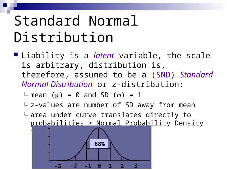
Liability is a latent variable, the scale is arbitrary, distribution is, therefore, assumed to be a (SND) Standard Normal Distribution or z-distribution: mean () = 0 and SD () = 1 z-values are number of SD away from mean area under curve translates directly to probabilities >

Normal Probability Density function ()

-3 3-1 0 1 2-2

68%

Z0 Area 0 .50 50%.2 .42 42%.4 .35 35%.6 .27 27%.8 .21 21% 1 .16 16%1.2 .12 12%1.4 .08 8%1.6 .06 6%1.8 .036 3.6%2 .023 2.3%2.2 .014 1.4%2.4 .008 .8%2.6 .005 .5%2.8 .003 .3%2.9 .002 .2%

-3 3z0

Area=P(z z0)

Cumulative Probability

Standard Normal Cumulative Probability in right-hand tail(For negative z values, areas are found by symmetry)

Univariate Normal Distribution

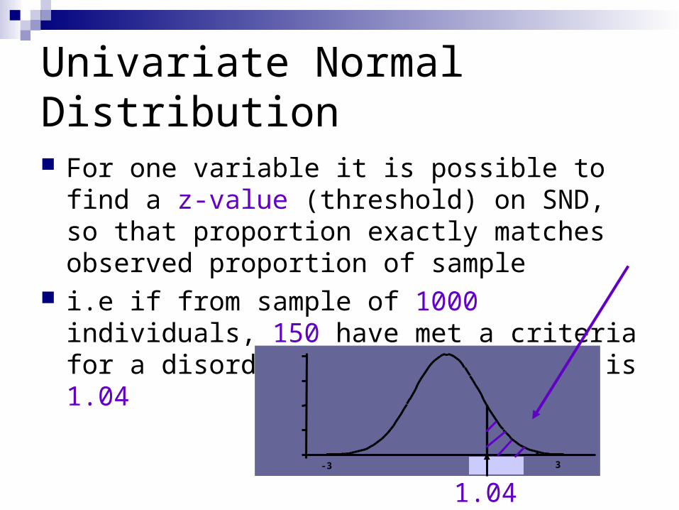
For one variable it is possible to find a z-value (threshold) on SND, so that proportion exactly matches observed proportion of sample

i.e if from sample of 1000 individuals, 150 have met a criteria for a disorder (15%): the z-value is 1.04

-3 3

1.04

Two Categorical Traits

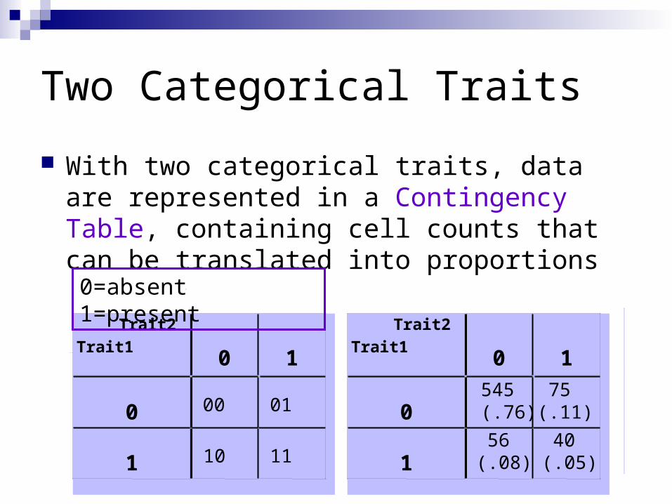
With two categorical traits, data are represented in a Contingency Table, containing cell counts that can be translated into proportions

Trait2Trait1

0 1

0 00 01

1 10 11

0=absent 1=present

Trait2Trait1

0 1

0 545 (.76)

75(.11)

1 56(.08)

40(.05)

Categorical Data for Twins

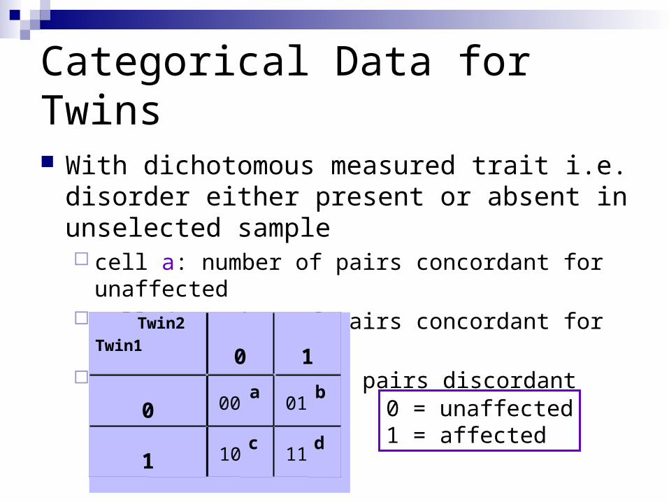
With dichotomous measured trait i.e. disorder either present or absent in unselected sample cell a: number of pairs concordant for unaffected cell d: number of pairs concordant for affected cell b/c: number of pairs discordant for disorder

0 = unaffected1 = affected

Twin2Twin1

0 1

0 00 a

01 b

1 10 c

11 d

Joint Liability Model for Twins

Assumed to follow a bivariate normal distribution Shape of bivariate normal distribution is

determined by correlation between traits Expected proportions under distribution can be

calculated by numerical integration with mathematical subroutines

R=.00 R=.90

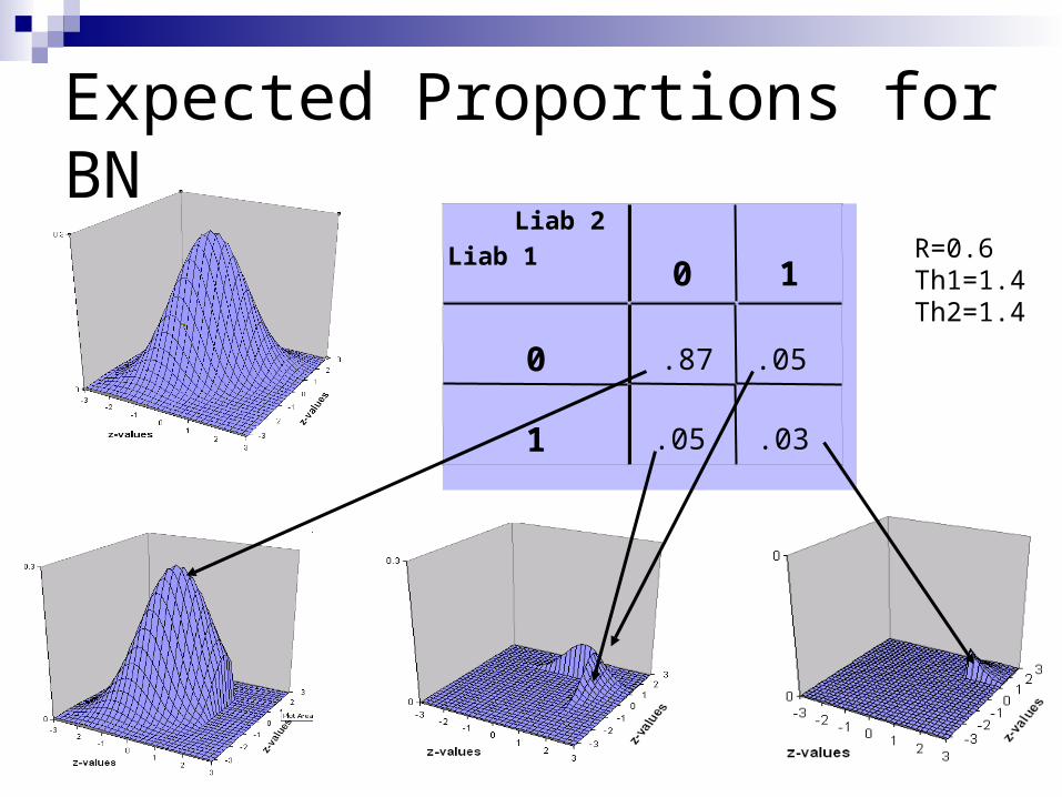
Liab 2Liab 1

0 1

0 .87

.05

1 .05

.03

R=0.6Th1=1.4Th2=1.4

Expected Proportions for BN

Correlated Dimensions

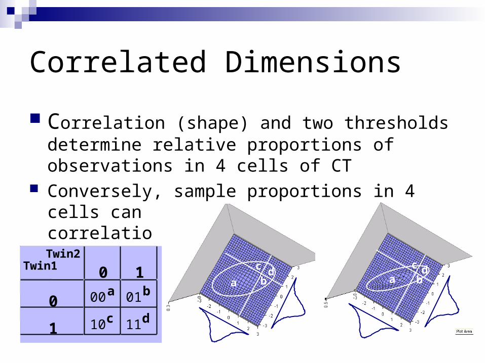
Correlation (shape) and two thresholds determine relative proportions of observations in 4 cells of CT

Conversely, sample proportions in 4 cells can be used to estimate correlation and thresholds

Twin2Twin1 0 1

0 00 a 01 b

1 10 c 11 d

ad

bc

acbd

ACE Liability Twin Model

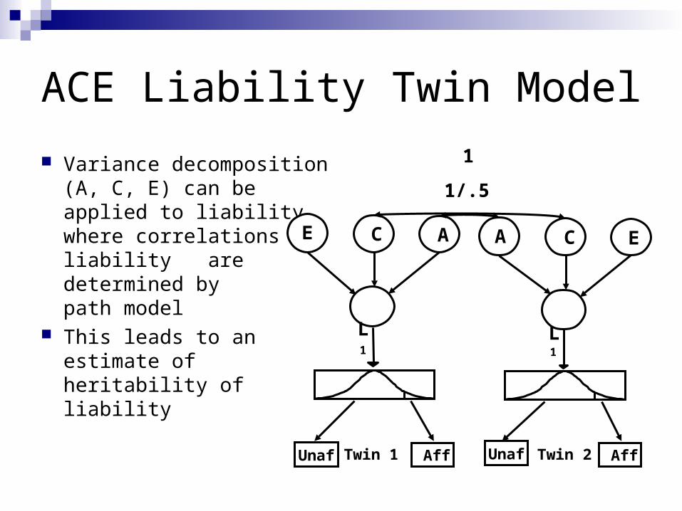
Variance decomposition (A, C, E) can be applied to liability, where correlations in liability are determined by path model

This leads to an estimate of heritability of liability

1

11

Twin 1

C EA

L

C AE

L

Twin 2Unaf ¯Aff Unaf ¯Aff

1/.5

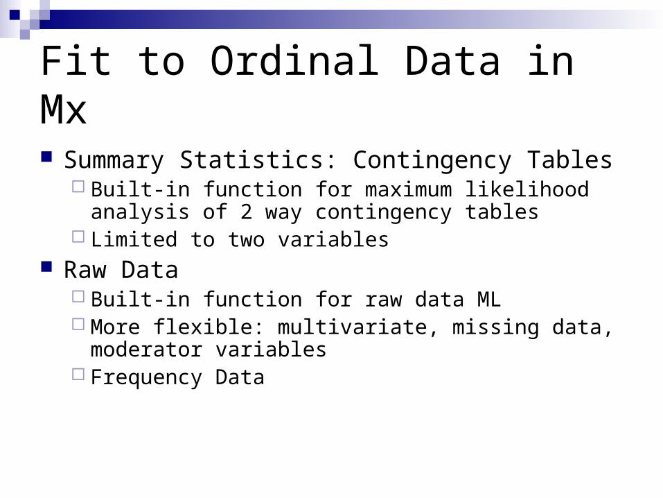
Fit to Ordinal Data in Mx

Summary Statistics: Contingency Tables Built-in function for maximum likelihood analysis of 2

way contingency tables Limited to two variables

Raw Data Built-in function for raw data ML More flexible: multivariate, missing data, moderator

variables Frequency Data

Model Fitting to CT

Fit function is twice the log-likelihood of the observed frequency data calculated as:

Where nij is the observed frequency in cell ij And pij is the expected proportion in cell ij

Expected proportions calculated by numerical integration of the bivariate normal over two dimensions: the liabilities for twin1 and twin2

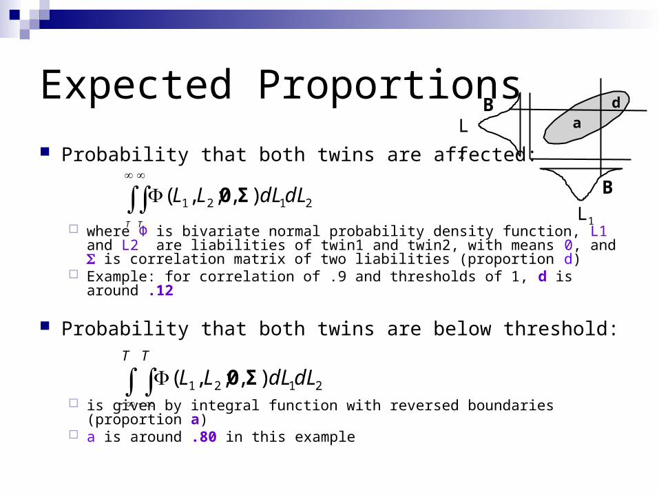
Expected Proportions

Probability that both twins are affected:

where Φ is bivariate normal probability density function, L1 and L2 are liabilities of twin1 and twin2, with means 0, and is correlation matrix of two liabilities (proportion d)

Example: for correlation of .9 and thresholds of 1, d is around .12

Probability that both twins are below threshold:

is given by integral function with reversed boundaries (proportion a) a is around .80 in this example

2121 ),;,( dLdLLLT T

Σ0

2121 ),;,( dLdLLLT T

Σ0

d

B

BL2

L1

a

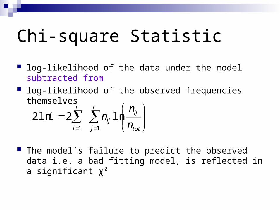
Chi-square Statistic

log-likelihood of the data under the model subtracted from

log-likelihood of the observed frequencies themselves

The model’s failure to predict the observed data i.e. a bad fitting model, is reflected in a significant χ²

tot

ijc

jij

r

i n

nnL ln2ln2

11

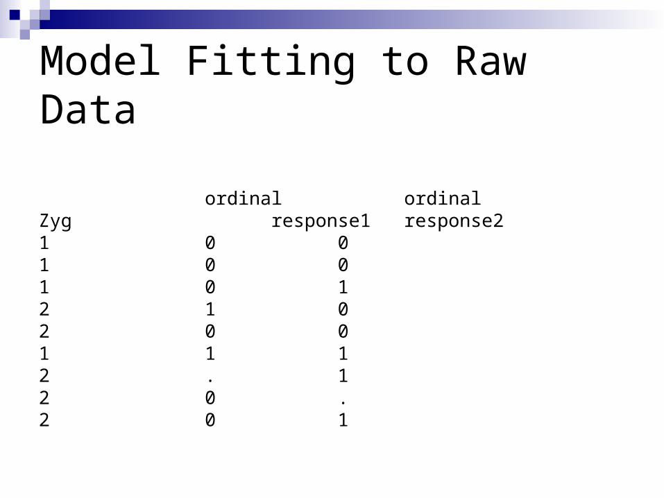
Model Fitting to Raw Data

ordinal ordinalZyg response1 response21 0 01 0 01 0 12 1 02 0 01 1 12 . 12 0 .2 0 1

Expected Proportions

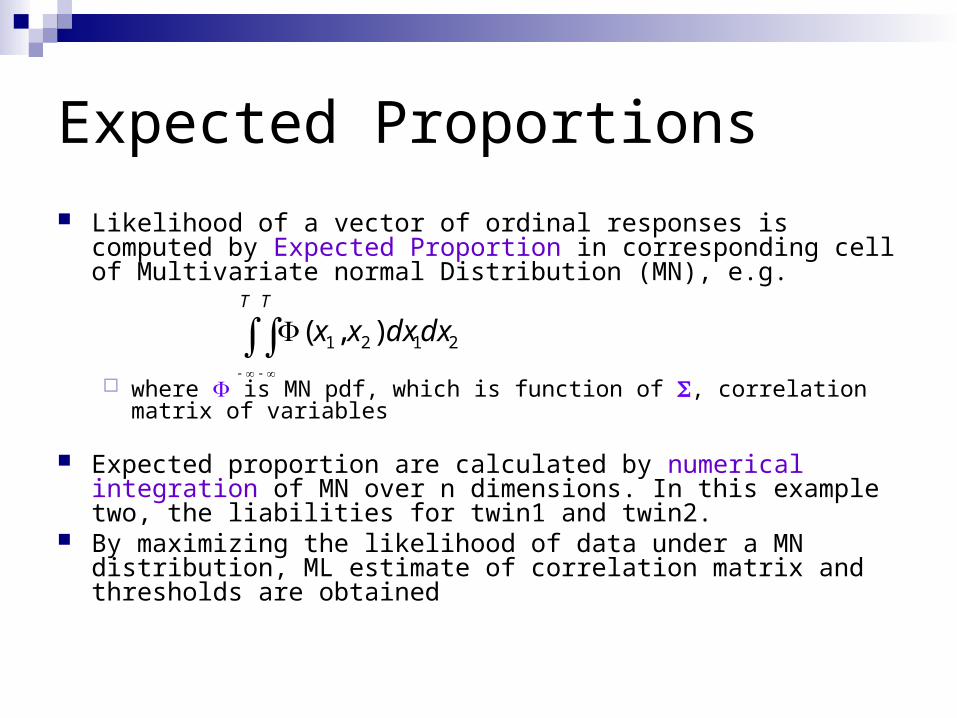
Likelihood of a vector of ordinal responses is computed by Expected Proportion in corresponding cell of Multivariate normal Distribution (MN), e.g.

where is MN pdf, which is function of , correlation matrix of variables

Expected proportion are calculated by numerical integration of MN over n dimensions. In this example two, the liabilities for twin1 and twin2.

By maximizing the likelihood of data under a MN distribution, ML estimate of correlation matrix and thresholds are obtained

2121 ),( dxdxxxT T

2121 ),( dxdxxxT

T

2121 ),( dxdxxxT

T

2121 ),( dxdxxxT T

2121 ),( dxdxxxT T

(0 1)(1 0)(0 0) (1 1)

Numerical Integration