Three Dimensional Microscopic Flow Simulation Across … · Three Dimensional Microscopic Flow Simulation Across ... simulations using the LBM. 2. ... Three Dimensional Microscopic

The Open Transport Phenomena Journal, 2009, 1, 35-44 35

1877-7295/09 2009 Bentham Open

Open Access

Three Dimensional Microscopic Flow Simulation Across the Interface of a Porous Wall and Clear Fluid by the Lattice Boltzmann Method

Kazuhiko Suga* and Yoshifumi Nishio

Department of Mechanical Engineering, Osaka Prefecture University, Sakai, Japan

Abstract: The effects of the porous medium on the flow in the interface region between a highly porous wall and clear fluid are discussed. Three dimensional laminar flows in the interface regions of foamed porous walls are microscopically simulated by the lattice Boltzmann method. The chosen porous structure is the body-centered-cubic or the unit cube structure whose porosity ranges 0.82-0.98. The velocity distribution in the interface regions show that the flow penetration into porous layer is very little and it decays until one pore-diameter depth from the interface. To describe the slip velocity distribution independently of the porous structure, the permeability Reynolds number and the friction velocity are confirmed to be representative scale parameters. The stress jump conditions across the interface are also examined with the simulation results. Although the obtained averaged wall friction of the porous interface is slightly lower than that of the solid smooth impermeable surface, the reduction is not significant due to the Reynolds stress arisen from the statistical averaging of the interfacial flow motions.

Keywords: porous wall, lattice Boltzmann method, laminar flow, slip velocity, flow penetration, stress jump condition, porous wall friction.

1. INTRODUCTION

Viscous fluid flows through porous media have been studied for many years after Darcy [1] since porous materials are so common in engineering fields as well as in the earth science. Once such porous materials are applied to fluid flows for guiding, filtering or controlling the fluid, the characteristics of flows over or around porous surfaces are also very important for designing the flow-devices. Accordingly, boundary layer flows over permeable walls have been of primary interests for many researchers.

Beavers and Joseph [2] studied on the effects of a porous medium on the flow in the interface region between the porous wall and clear fluid (named “interface region” hereafter). They measured mass flow rates over permeable beds in laminar flow conditions and found that the mass flow rates increased compared with those in impermeable cases. Many other following studies [3-9] also focused on the laminar flow regime experimentally and numerically since the flow physics is rather complicated and controversial even in laminar flows. In fact, the effects of flow penetration into porous layers are still not fully understood. Gupte and Advani [7] performed mean flow measurements in the interface region of fibrous mats using a laser Doppler anemometry. They reported that the flow penetration into the porous layer was stronger than that estimated semi-theoretically in the laminar flow regime. Since their measurements were performed at the slits between fibrous mats, the reported results might not show the pure penetration effects. On the contrary, James and Davis [8] reported numerically that the external flow penetrated the fibrous porous medium very little.

*Address correspondence to this author at the Department of Mechanical

Engineering, Osaka Prefecture University, Sakai, Japan; Tel: +81 72 254

9224; Fax: +81 72 254 9904; E-mail: [email protected]

The slip velocity at the interface is also one of the issues. On the porous interface, the fluid motion is not totally damped having non-zero statistical tangential velocity component. Since this slip velocity is required to solve the momentum equations over the interface as a boundary condition, Beavers and Joseph [2] proposed a condition that is a function of the permeability and the Darcy velocity of the porous media. This condition was supported by many studies [4,5,10]. Ochoa-Tapia and Whitaker [6] proposed another relation introducing a jump condition of the stress distribution across the interface. Both of the conditions require experimental measurements for determining their coefficients. Thus, to answer the question of which condition is better or more useful representation, discussions using measured or simulated data are essential.

Another important issue is the friction of the porous surfaces. In laminar flow regimes, the aforementioned work by Beavers and Joseph

[2] reported that the friction over the

porous walls reduced due to the porosity. However, Zagni and Smith [11] and Zippe and Graf [12] experimentally found that the friction factors of turbulent flows over permeable beds became higher than those over impermeable walls with the same surface roughness. Kong and Schetz [13] observed that the increase of the skin friction was due to the combined effects of roughness and porosity. Thus, the mechanism to produce such a difference depending on the flow regimes is still unknown.

In order to understand the flow characteristics in the interface regions, it is necessary to obtain the detailed flow profiles in the interface region. However, measuring flow profiles across the interface region is very difficult even with the latest measurement techniques. Thus, one can expect that numerical analyses can provide useful information instead. The recently emerged lattice Boltzmann method (LBM)

[14,15] has become powerful tool for simulating flows inside porous media [16-18] due to its coding simplicity of the

36 The Open Transport Phenomena Journal, 2009, Volume 1 Suga and Nishio

method for complicated flow geometries. Therefore, in order to understand and discuss the flow characteristics such as the flow penetration, the slip velocity, the stress jump condition and the friction of the porous interfaces in laminar flow regimes, the present study has performed numerical simulations using the LBM.

2. NUMERICAL METHODS

2.1. Lattice Boltzmann Method

The presently used LBM employs the single-relaxation-time (SRT) Bhatnagar-Gross- Krook (BGK) [19] model which is briefly described below.

The lattice Boltzmann method for flow simulation by the SRT BGK model may be written as

f (r + et, t +

t) = f (r, t)

f (r, t) f eq (r, t),

( = 0,1,2, ,Q 1),

(1)

where f (r, t) is the density distribution function along the

direction at the lattice site r at time t , e is the discrete

velocity, t

is the time step and is the dimensionless

relaxation time ( = 1 is applied in this study). The

equilibrium distribution function determined by the fluid

density and momentum is

f eq= w 1+

e u

cS

2+

(e u)2 cS

2u

2

2cS

4, (2)

where w is the weight coefficient and

c

S is the sound

speed. Once the density distribution function is known, the

density , the velocity u, the pressure p and the kinematic

viscosity are obtained from the conservation laws and the

equation of state:

= f , u = f c , p = cS

2, = c

S

2 1

2t. (3)

In the present study, the D3Q19 discrete velocity model shown in Fig. (1), whose parameters [20] are listed in Table 1, is employed.

At the solid wall boundaries, the usual half-way bounce-

back (HWBB) method [18] is employed. (In [18], the

HWBB is called the perfect bounce-back.) Fig. (1b)

illustrates the procedures of the HWBB method in a

(a)

(b)

(c)

Fig.(1). Discrete velocity and solid wall boundary models: (a)

D3Q19 discrete velocity model, (b) half-way bounce back, (c)

representation of a curved surface by the half-way bounce-back

boundary condition.

Table 1. Parameters of the Discrete Velocity Model of D3Q19

c

S

2

e

w

1/3

(0,0,0)

( ±1,0 ,0),(0, ±1 ,0),(0,0, ±1 )

( ±1,±1 ,0),( ±1 ,0, 1± ),(0,

±1,±1 )

12/36( = 0)

2/36( = 1, ,6)

1/36( = 7, ,18)

0

Three Dimensional Microscopic Flow Simulation Across the Interface The Open Transport Phenomena Journal, 2009, Volume 1 37

one-dimensional setting. In this case, since the boundary x

W

is located at the middle between nodes x

A and

x

B,

( | x

Ax

W| /

| x

Ax

B|= 1 / 2 ), the particle at node A

x

travels and collides with the wall at x

W and reverses its

momentum (the collision process completes instantly), then

travels back to Ax . Thus, the incoming distribution function

is simply equal to the corresponding outgoing one with the

opposite momentum. As discussed in [21] the special error

convergence of the HWBB method is first order and its

representation of a curved surface is step-like as shown in

Fig. (1c). Although HWBB condition is less accurate than

the other elaborate method, it is computationally efficient

and generally gives reasonable results [22]. Indeed, the

authors’ group confirmed that it was reasonably accurate to

reproduce flow characteristics in porous media [23].

2.2. Models of Foamed Porous Media

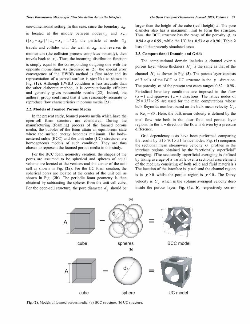
In the present study, foamed porous media which have the open-cell foam structure are considered. During the manufacturing (foaming) process of the foamed porous media, the bubbles of the foam attain an equilibrium state where the surface energy becomes minimum. The body-centered-cubic (BCC) and the unit cube (UC) structures are homogeneous models of such condition. They are thus chosen to represent the foamed porous media in this study.

For the BCC foam geometry creation, the shapes of the

pores are assumed to be spherical and spheres of equal

volume are located at the vertices and the center of the unit

cell as shown in Fig. (2a). For the UC foam creation, the

spherical pores are located at the center of the unit cell as

shown in Fig. (2b). The periodic foam geometry is then

obtained by subtracting the spheres from the unit cell cube.

For the open-cell structure, the pore diameter d

p should be

larger than the height of the cube (:cell height) A. The pore

diameter also has a maximum limit to form the structure.

Thus, the BCC structure has the range of the porosity as

0.94 < < 0.99 , while the UC has

0.53 < < 0.96 . Table 2

lists all the presently simulated cases.

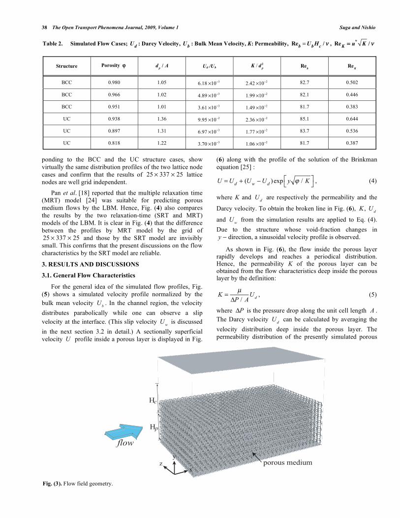
2.3. Computational Domain and Grids

The computational domain includes a channel over a

porous layer whose thickness H

p is the same as that of the

channel H

c as shown in Fig. (3). The porous layer consists

of 7 cells of the BCC or UC structure in the y direction.

The porosity of the present test cases ranges 0.82 0.98 .

Periodical boundary conditions are imposed in the flow

( x ) and spanwise ( z ) directions. The lattice nodes of

25 337 25 are used for the main computations whose

bulk Reynolds number, based on the bulk mean velocity U

b,

is Re

b= 80 . Here, the bulk mean velocity is defined by the

total flow rate both in the clear fluid and porous layer

regions. In the x direction, the flow is driven by a pressure

difference.

Grid dependency tests have been performed comparing

the results by 51 701 51 lattice nodes. Fig. (4) compares

the sectional mean streamwise velocity U profiles in the

interface regions obtained by the “sectionally superficial”

averaging. (The sectionally superficial averaging is defined

by taking average of a variable over a sectional area element

of the medium consisting of both solid and fluid materials.)

The location of the interface is y = 0 and the channel region

is in y 0 whilst the porous region is

y 0 . The Darcy

velocity is U

d which is the volume averaged velocity deep

inside the porous layer. Fig. (4a, b), respectively corres-

(a)

(b)

Fig. (2). Models of foamed porous media: (a) BCC structure, (b) UC structure.

cube spheres BCC model

d

A

cube sphere UC model

dp

A


ponding to the BCC and the UC structure cases, show

virtually the same distribution profiles of the two lattice node

cases and confirm that the results of 25 337 25 lattice

nodes are well grid independent.

Pan et al. [18] reported that the multiple relaxation time

(MRT) model [24] was suitable for predicting porous

medium flows by the LBM. Hence, Fig. (4) also compares

the results by the two relaxation-time (SRT and MRT)

models of the LBM. It is clear in Fig. (4) that the difference

between the profiles by MRT model by the grid of

25 337 25 and those by the SRT model are invisibly

small. This confirms that the present discussions on the flow

characteristics by the SRT model are reliable.

3. RESULTS AND DISCUSSIONS

3.1. General Flow Characteristics

For the general idea of the simulated flow profiles, Fig.

(5) shows a simulated velocity profile normalized by the

bulk mean velocity U

b. In the channel region, the velocity

distributes parabolically while one can observe a slip

velocity at the interface. (This slip velocity U

w is discussed

in the next section 3.2 in detail.) A sectionally superficial

velocity U profile inside a porous layer is displayed in Fig.

(6) along with the profile of the solution of the Brinkman

equation [25] :

U = U

d+ (U

wU

d) exp y / K , (4)

where K and U

d are respectively the permeability and the

Darcy velocity. To obtain the broken line in Fig. (6), K , U

d

and U

w from the simulation results are applied to Eq. (4).

Due to the structure whose void-fraction changes in

y direction, a sinusoidal velocity profile is observed.

As shown in Fig. (6), the flow inside the porous layer rapidly develops and reaches a periodical distribution. Hence, the permeability K of the porous layer can be obtained from the flow characteristics deep inside the porous layer by the definition:

K =μ

P / AU

d, (5)

where P is the pressure drop along the unit cell length A .

The Darcy velocity U

d can be calculated by averaging the

velocity distribution deep inside the porous layer. The

permeability distribution of the presently simulated porous

Table 2. Simulated Flow Cases; U

d: Darcy Velocity,

U

b: Bulk Mean Velocity, K: Permeability,

Re

b=U

bH

c/ ,

Re

K= u

*K /

Structure Porosity d

p/ A Ud /Ub

K / d

p

2

Re

b

Re

K

BCC 0.980 1.05 6.18 103

2.42 102

82.7 0.502

BCC 0.966 1.02 4.89 103

1.99 102

82.1 0.446

BCC 0.951 1.01 3.61 103

1.49 102

81.7 0.383

UC 0.938 1.36 9.95 102

2.36 102

85.1 0.644

UC 0.897 1.31 6.97 103

1.77 102

83.7 0.536

UC 0.818 1.22 3.70 103

1.06 102

81.7 0.387

Fig. (3). Flow field geometry.

y

xz

flow

H

H

c

p

porous medium


layers are shown in Fig. (7). The normalized permeability

K / d2 is defined after Bhattacharya et al. [26]. The

microscopic characteristic length d of foamed porous media

by Du Plessis et al. [27] is determined with the pore diameter

d

p as

d = 2 1 / (3 )d

p. (6)

(a)

(b)

Fig. (4). Grid and relaxation-time model dependency: (a) BCC

structure, (b) UC structure.

As shown in Fig. (7), the presently obtained permeability of

the BCC structure accords well with the experimental data

[26] of foamed porous metals. This confirms that the BCC

structure is a reasonable model for foamed porous media and

also the present numerical methods are reliable enough.

Since the permeability of the UC structure is higher than the

experimental data, it implies that such a structure is not very

good representation of the experimentally chosen foamed

materials. Although both the BCC and UC cases show the

increase of the permeability with the increase of the porosity,

one can see an obvious difference between the two structures.

This clearly implies that the permeability is subjected to both

the porosity and the structure. Note that in the preliminary

computations, it has been confirmed that the normalized

values of the flow characteristics such as the permeability

K / d

p

2 and the Darcy velocity

U

d/ U

b do not vary in the

Reynolds number range: 20 Re

b200 .

Fig. (5). Velocity profile.

Fig. (6). Sectionally superficial velocity profile in the porous

region.

Fig. (7). Computed permeability distribution.

As discussed with Fig. (6), the flow distribution depends on the phase of the local void-fraction. Although the simulated porous media have perfectly regular homogeneous structure, many phase-positions can be defined at the


surface. Thus, in order to obtain reasonably general flow characteristics of the structure, averaging several different cases of the surface phase-position is applied. Although there are an infinite number of phases to determine the porous interface, 2 types of the interface position (1, 1/4) are applied for the BCC structure as shown in Fig. (8). They represent 2 main phase-positions which are opposite phases to each other. Note that the phases of position 3/4 and 1/2 are the same as those of 1/4 and 1, respectively. For the UC structure, 4 types of the position (1, 3/4, 1/2, 1/4) as in Fig. (8) are applied for averaging. In the following discussions, all velocity profiles are obtained by this averaging process.

Fig. (8). Interface positions.

With this averaging, the sinusoidal velocity profile is smoothed out as shown in Fig. (9). In fact, the velocity profile reasonably accords with the profile of the solution of the Brinkman equation, Eq.(4). This indicates that the general velocity distribution and the flow penetration inside the present porous media can be reasonably estimated by the Brinkman equation if the correct interface velocity is given.

Fig. (9). Averaged velocity profile of 2 different phases of the BCC

structure.

3.2. Flow Penetration and Slip Velocity

As shown in Fig. (9), the flow penetration region is

defined as the region where the averaged velocity is 5%

greater than the Darcy velocity U

d in this study. The

penetration length is the thickness of this penetration region.

The obtained penetration length l

p is plotted in Fig. (10). It

is clear that the penetration length generally increases with

the porosity. However, the maximum penetration length is

less than the pore diameter d

p. This tendency is also

observed in a finer porous layer which has the same

thickness but 28 layers of the cells in the extra simulations

by 25 1345 25 lattice nodes. The present results support

the numerical study of James and Davis [8] which reported

that the external flow penetrated the porous layer (consisting

of circular cylinder arrays) very little even for sparse arrays

of circular cylinders.

Fig. (10). Flow penetration length.

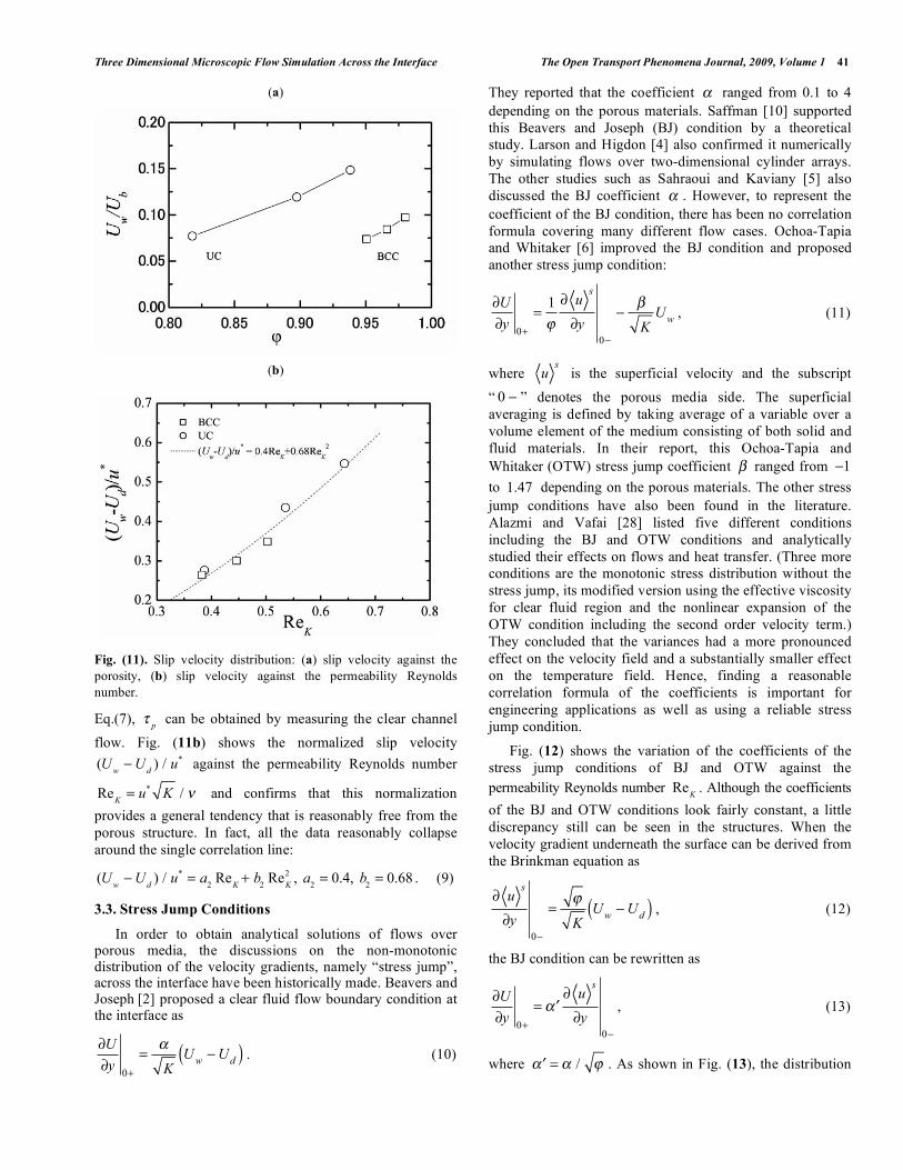
Fig. (11a) shows the slip velocity against the porosity.

Although the slip velocity increases with the porosity, it

strongly depends on the porous structure. James and Davis

[8] normalized the slip velocity using the permeability and

the velocity gradient as U

w/ ( K dU / dy) and discussed its

behavior against the porosity. However, in their figures, it is

difficult to find a simple correlation to represent the slip

velocity distribution. Gupte and Advani [7] also discussed

the normalized slip velocity U

w/ U (

U is the free stream

velocity) against the permeability. Although a linear

correlation profile was observed, their experimental points

plotted were only three. Thus, in order to find a general

distribution profile of the slip velocity independent of the

structure, the normalization by the friction velocity *u and

the permeability is presently considered. (Generally, the

friction velocity is a representative scale parameter for the

boundary layer.) The friction velocity u

*=

p/ can be

obtained from the porous wall friction:

p= H

c

dP

dx s, (7)

where

s= μ dU / dy

y= Hc

. Note that the present porous

wall friction includes all the porous interface effects and thus

p= (μ + μ

eff)

U

y0+

, (8)

where μ

eff is the effective viscosity arising from the

statistical handling of the interface flows and the subscript

“ 0 + ” denotes the clear fluid side. With the definition by


(a)

(b)

Fig. (11). Slip velocity distribution: (a) slip velocity against the

porosity, (b) slip velocity against the permeability Reynolds

number.

Eq.(7), p

can be obtained by measuring the clear channel

flow. Fig. (11b) shows the normalized slip velocity

(U

wU

d) / u

* against the permeability Reynolds number

Re

K= u

*K / and confirms that this normalization

provides a general tendency that is reasonably free from the

porous structure. In fact, all the data reasonably collapse

around the single correlation line:

(U

wU

d) / u

*= a

2Re

K+ b

2Re

K

2 , a2= 0.4, b

2= 0.68 . (9)

3.3. Stress Jump Conditions

In order to obtain analytical solutions of flows over porous media, the discussions on the non-monotonic distribution of the velocity gradients, namely “stress jump”, across the interface have been historically made. Beavers and Joseph

[2] proposed a clear fluid flow boundary condition at

the interface as

U

y0+

=K

Uw

Ud( ) . (10)

They reported that the coefficient ranged from 0.1 to 4

depending on the porous materials. Saffman [10] supported

this Beavers and Joseph (BJ) condition by a theoretical

study. Larson and Higdon [4] also confirmed it numerically

by simulating flows over two-dimensional cylinder arrays.

The other studies such as Sahraoui and Kaviany [5] also

discussed the BJ coefficient . However, to represent the

coefficient of the BJ condition, there has been no correlation

formula covering many different flow cases. Ochoa-Tapia

and Whitaker [6] improved the BJ condition and proposed

another stress jump condition:

U

y0+

=1 u

s

y0

KU

w, (11)

where

us

is the superficial velocity and the subscript

“ 0 ” denotes the porous media side. The superficial

averaging is defined by taking average of a variable over a

volume element of the medium consisting of both solid and

fluid materials. In their report, this Ochoa-Tapia and

Whitaker (OTW) stress jump coefficient ranged from 1

to 1.47 depending on the porous materials. The other stress

jump conditions have also been found in the literature.

Alazmi and Vafai [28] listed five different conditions

including the BJ and OTW conditions and analytically

studied their effects on flows and heat transfer. (Three more

conditions are the monotonic stress distribution without the

stress jump, its modified version using the effective viscosity

for clear fluid region and the nonlinear expansion of the

OTW condition including the second order velocity term.)

They concluded that the variances had a more pronounced

effect on the velocity field and a substantially smaller effect

on the temperature field. Hence, finding a reasonable

correlation formula of the coefficients is important for

engineering applications as well as using a reliable stress

jump condition.

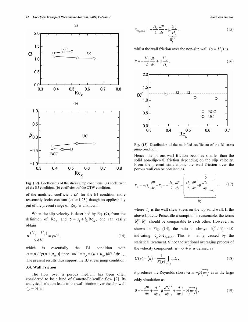
Fig. (12) shows the variation of the coefficients of the

stress jump conditions of BJ and OTW against the

permeability Reynolds number Re

K. Although the coefficients

of the BJ and OTW conditions look fairly constant, a little

discrepancy still can be seen in the structures. When the

velocity gradient underneath the surface can be derived from

the Brinkman equation as

us

y0

=K

Uw

Ud( ) , (12)

the BJ condition can be rewritten as

U

y0+

=

us

y0

, (13)

where

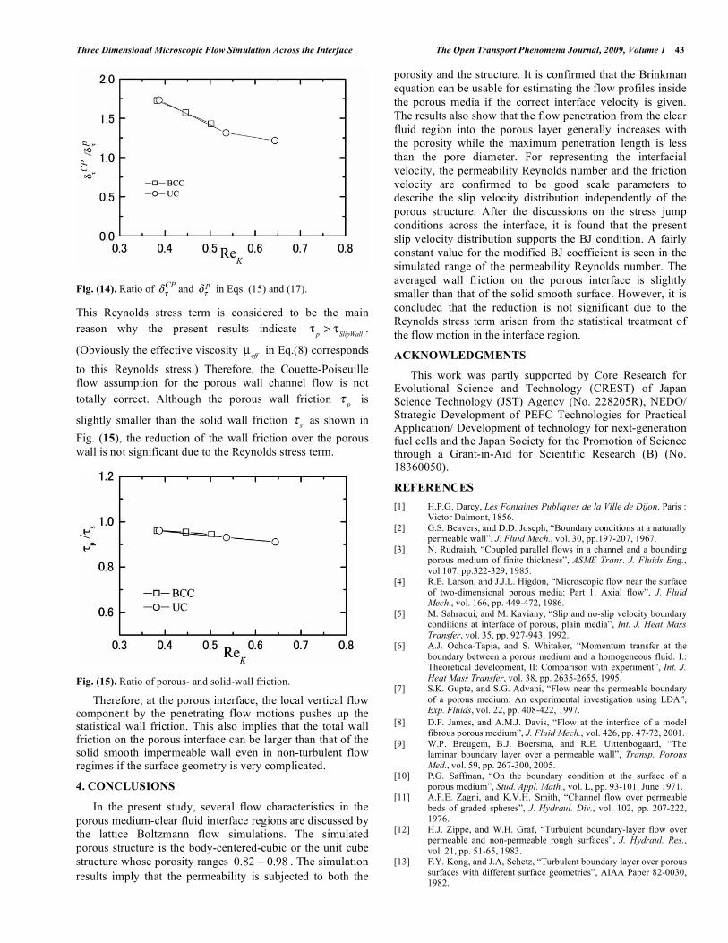
= / . As shown in Fig. (13), the distribution


(a)

(b)

Fig. (12). Coefficients of the stress jump conditions: (a) coefficient

of the BJ condition, (b) coefficient of the OTW condition.

of the modified coefficient for the BJ condition more

reasonably looks constant ( 1.25 ) though its applicability

out of the present range of Re

K is unknown.

When the slip velocity is described by Eq. (9), from the

definition of Re

K and

= a

2+ b

2Re

K, one can easily

obtain

μ(U

wU

d)

K

= u*2 , (14)

which is essentially the BJ condition with

= μ / [ (μ + μ

eff)] since

u*2

=p= (μ + μ

eff) U / y |

+0.

The present results thus support the BJ stress jump condition.

3.4. Wall Friction

The flow over a porous medium has been often

considered to be a kind of Couette-Poiseuille flow [2]. Its

analytical solution leads to the wall friction over the slip wall

( y = 0) as

SlipWall=

Hc

2

dP

dxμ

Uw

Hc

CP

, (15)

whilst the wall friction over the non-slip wall ( y = H

c) is

=H

c

2

dP

dx+ μ

Uw

Hc

. (16)

Fig. (13). Distribution of the modified coefficient of the BJ stress

jump condition.

Hence, the porous-wall friction becomes smaller than the solid non-slip-wall friction depending on the slip velocity. From the present simulations, the wall friction over the porous wall can be obtained as

p= H

c

dP

dx s=

Hc

2

dP

dx

Hc

2

dP

dxμ

dU

dyy=H

c

s

p

, (17)

where s

is the wall shear stress on the top solid wall. If the

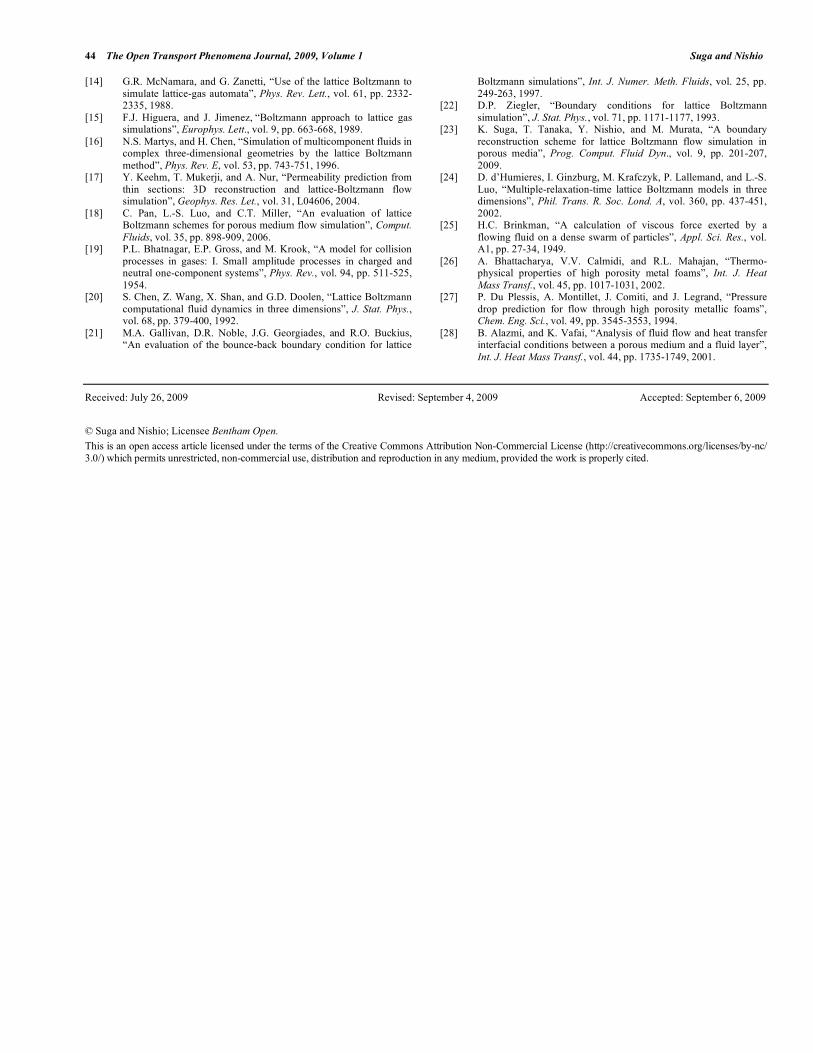
above Couette-Poiseuille assumption is reasonable, the terms

CP

,p should be comparable to each other. However, as

shown in Fig. (14), the ratio is always

CP/

p >1.0

indicating p

>SlipWall

. This is mainly caused by the

statistical treatment. Since the sectional averaging process of

the velocity component: u = U + u is defined as

U ( y) = u =1

S( y)uds

S ( y )

, (18)

it produces the Reynolds stress term

uv as in the large

eddy simulation as

0 =dP

dx+

d

dyμ

dU

dy+

d

dyuv( ) . (19)


Fig. (14). Ratio of

CP and

p in Eqs. (15) and (17).

This Reynolds stress term is considered to be the main

reason why the present results indicate p

>SlipWall

.

(Obviously the effective viscosity μ

eff in Eq.(8) corresponds

to this Reynolds stress.) Therefore, the Couette-Poiseuille

flow assumption for the porous wall channel flow is not

totally correct. Although the porous wall friction p

is

slightly smaller than the solid wall friction s

as shown in

Fig. (15), the reduction of the wall friction over the porous

wall is not significant due to the Reynolds stress term.

Fig. (15). Ratio of porous- and solid-wall friction.

Therefore, at the porous interface, the local vertical flow component by the penetrating flow motions pushes up the statistical wall friction. This also implies that the total wall friction on the porous interface can be larger than that of the solid smooth impermeable wall even in non-turbulent flow regimes if the surface geometry is very complicated.

4. CONCLUSIONS

In the present study, several flow characteristics in the

porous medium-clear fluid interface regions are discussed by

the lattice Boltzmann flow simulations. The simulated

porous structure is the body-centered-cubic or the unit cube

structure whose porosity ranges 0.82 0.98 . The simulation

results imply that the permeability is subjected to both the

porosity and the structure. It is confirmed that the Brinkman

equation can be usable for estimating the flow profiles inside

the porous media if the correct interface velocity is given.

The results also show that the flow penetration from the clear

fluid region into the porous layer generally increases with

the porosity while the maximum penetration length is less

than the pore diameter. For representing the interfacial

velocity, the permeability Reynolds number and the friction

velocity are confirmed to be good scale parameters to

describe the slip velocity distribution independently of the

porous structure. After the discussions on the stress jump

conditions across the interface, it is found that the present

slip velocity distribution supports the BJ condition. A fairly

constant value for the modified BJ coefficient is seen in the

simulated range of the permeability Reynolds number. The

averaged wall friction on the porous interface is slightly

smaller than that of the solid smooth surface. However, it is

concluded that the reduction is not significant due to the

Reynolds stress term arisen from the statistical treatment of

the flow motion in the interface region.

ACKNOWLEDGMENTS

This work was partly supported by Core Research for Evolutional Science and Technology (CREST) of Japan Science Technology (JST) Agency (No. 228205R), NEDO/ Strategic Development of PEFC Technologies for Practical Application/ Development of technology for next-generation fuel cells and the Japan Society for the Promotion of Science through a Grant-in-Aid for Scientific Research (B) (No. 18360050).

REFERENCES

[1] H.P.G. Darcy, Les Fontaines Publiques de la Ville de Dijon. Paris : Victor Dalmont, 1856.

[2] G.S. Beavers, and D.D. Joseph, “Boundary conditions at a naturally permeable wall”, J. Fluid Mech., vol. 30, pp.197-207, 1967.

[3] N. Rudraiah, “Coupled parallel flows in a channel and a bounding porous medium of finite thickness”, ASME Trans. J. Fluids Eng.,

vol.107, pp.322-329, 1985. [4] R.E. Larson, and J.J.L. Higdon, “Microscopic flow near the surface

of two-dimensional porous media: Part 1. Axial flow”, J. Fluid Mech., vol. 166, pp. 449-472, 1986.

[5] M. Sahraoui, and M. Kaviany, “Slip and no-slip velocity boundary conditions at interface of porous, plain media”, Int. J. Heat Mass

Transfer, vol. 35, pp. 927-943, 1992. [6] A.J. Ochoa-Tapia, and S. Whitaker, “Momentum transfer at the

boundary between a porous medium and a homogeneous fluid. I.: Theoretical development, II: Comparison with experiment”, Int. J.

Heat Mass Transfer, vol. 38, pp. 2635-2655, 1995. [7] S.K. Gupte, and S.G. Advani, “Flow near the permeable boundary

of a porous medium: An experimental investigation using LDA”, Exp. Fluids, vol. 22, pp. 408-422, 1997.

[8] D.F. James, and A.M.J. Davis, “Flow at the interface of a model fibrous porous medium”, J. Fluid Mech., vol. 426, pp. 47-72, 2001.

[9] W.P. Breugem, B.J. Boersma, and R.E. Uittenbogaard, “The laminar boundary layer over a permeable wall”, Transp. Porous

Med., vol. 59, pp. 267-300, 2005. [10] P.G. Saffman, “On the boundary condition at the surface of a

porous medium”, Stud. Appl. Math., vol. L, pp. 93-101, June 1971. [11] A.F.E. Zagni, and K.V.H. Smith, “Channel flow over permeable

beds of graded spheres”, J. Hydraul. Div., vol. 102, pp. 207-222, 1976.

[12] H.J. Zippe, and W.H. Graf, “Turbulent boundary-layer flow over permeable and non-permeable rough surfaces”, J. Hydraul. Res.,

vol. 21, pp. 51-65, 1983. [13] F.Y. Kong, and J.A, Schetz, “Turbulent boundary layer over porous

surfaces with different surface geometries”, AIAA Paper 82-0030, 1982.


[14] G.R. McNamara, and G. Zanetti, “Use of the lattice Boltzmann to

simulate lattice-gas automata”, Phys. Rev. Lett., vol. 61, pp. 2332-2335, 1988.

[15] F.J. Higuera, and J. Jimenez, “Boltzmann approach to lattice gas simulations”, Europhys. Lett., vol. 9, pp. 663-668, 1989.

[16] N.S. Martys, and H. Chen, “Simulation of multicomponent fluids in complex three-dimensional geometries by the lattice Boltzmann

method”, Phys. Rev. E, vol. 53, pp. 743-751, 1996. [17] Y. Keehm, T. Mukerji, and A. Nur, “Permeability prediction from

thin sections: 3D reconstruction and lattice-Boltzmann flow simulation”, Geophys. Res. Let., vol. 31, L04606, 2004.

[18] C. Pan, L.-S. Luo, and C.T. Miller, “An evaluation of lattice Boltzmann schemes for porous medium flow simulation”, Comput.

Fluids, vol. 35, pp. 898-909, 2006. [19] P.L. Bhatnagar, E.P. Gross, and M. Krook, “A model for collision

processes in gases: I. Small amplitude processes in charged and neutral one-component systems”, Phys. Rev., vol. 94, pp. 511-525,

1954. [20] S. Chen, Z. Wang, X. Shan, and G.D. Doolen, “Lattice Boltzmann

computational fluid dynamics in three dimensions”, J. Stat. Phys., vol. 68, pp. 379-400, 1992.

[21] M.A. Gallivan, D.R. Noble, J.G. Georgiades, and R.O. Buckius, “An evaluation of the bounce-back boundary condition for lattice

Boltzmann simulations”, Int. J. Numer. Meth. Fluids, vol. 25, pp.

249-263, 1997. [22] D.P. Ziegler, “Boundary conditions for lattice Boltzmann

simulation”, J. Stat. Phys., vol. 71, pp. 1171-1177, 1993. [23] K. Suga, T. Tanaka, Y. Nishio, and M. Murata, “A boundary

reconstruction scheme for lattice Boltzmann flow simulation in porous media”, Prog. Comput. Fluid Dyn., vol. 9, pp. 201-207,

2009. [24] D. d’Humieres, I. Ginzburg, M. Krafczyk, P. Lallemand, and L.-S.

Luo, “Multiple-relaxation-time lattice Boltzmann models in three dimensions”, Phil. Trans. R. Soc. Lond. A, vol. 360, pp. 437-451,

2002. [25] H.C. Brinkman, “A calculation of viscous force exerted by a

flowing fluid on a dense swarm of particles”, Appl. Sci. Res., vol. A1, pp. 27-34, 1949.

[26] A. Bhattacharya, V.V. Calmidi, and R.L. Mahajan, “Thermo-physical properties of high porosity metal foams”, Int. J. Heat

Mass Transf., vol. 45, pp. 1017-1031, 2002. [27] P. Du Plessis, A. Montillet, J. Comiti, and J. Legrand, “Pressure

drop prediction for flow through high porosity metallic foams”, Chem. Eng. Sci., vol. 49, pp. 3545-3553, 1994.

[28] B. Alazmi, and K. Vafai, “Analysis of fluid flow and heat transfer interfacial conditions between a porous medium and a fluid layer”,

Int. J. Heat Mass Transf., vol. 44, pp. 1735-1749, 2001.

Received: July 26, 2009 Revised: September 4, 2009 Accepted: September 6, 2009

© Suga and Nishio; Licensee Bentham Open.

This is an open access article licensed under the terms of the Creative Commons Attribution Non-Commercial License (http://creativecommons.org/licenses/by-nc/

3.0/) which permits unrestricted, non-commercial use, distribution and reproduction in any medium, provided the work is properly cited.

Documents

Three Dimensional Microscopic Flow Simulation Across … · Three Dimensional Microscopic Flow Simulation Across ... simulations using the LBM. 2. ... Three Dimensional Microscopic