Thirty Years with EoS/GE Models - What Have We Learned?orbit.dtu.dk/files/7743030/ie2015119.pdf · Thirty Years with EoS/GE Models ... Thirty Years with EoS/GE Models What Have We

General rights Copyright and moral rights for the publications made accessible in the public portal are retained by the authors and/or other copyright owners and it is a condition of accessing publications that users recognise and abide by the legal requirements associated with these rights.

• Users may download and print one copy of any publication from the public portal for the purpose of private study or research. • You may not further distribute the material or use it for any profit-making activity or commercial gain • You may freely distribute the URL identifying the publication in the public portal

If you believe that this document breaches copyright please contact us providing details, and we will remove access to the work immediately and investigate your claim.

Downloaded from orbit.dtu.dk on: Jul 12, 2018

Thirty Years with EoS/GE Models - What Have We Learned?

Kontogeorgis, Georgios; Coutsikos, Philippos

Published in:Industrial & Engineering Chemistry Research

Link to article, DOI:10.1021/ie2015119

Publication date:2012

Document VersionPublisher's PDF, also known as Version of record

Link back to DTU Orbit

Citation (APA):Kontogeorgis, G. M., & Coutsikos, P. (2012). Thirty Years with EoS/GE Models - What Have We Learned?Industrial & Engineering Chemistry Research, 51(11), 4119-4142. DOI: 10.1021/ie2015119

http://dx.doi.org/10.1021/ie2015119

http://orbit.dtu.dk/en/publications/thirty-years-with-eosge-models--what-have-we-learned(71f22db0-9d72-4206-8ae7-351015e36935).html

Thirty Years with EoS/GE ModelsWhat Have We Learned?Georgios M. Kontogeorgis* and Philippos Coutsikos

Centre for Energy Resources Engineering (CERE), Department of Chemical and Biochemical Engineering,Technical University of Denmark, DK-2800, Lyngby, Denmark

ABSTRACT: Thirty years of research and the use of EoS/GE mixing rules in cubic equations of state are reviewed. The mostpopular approaches are presented both from the derivation and application points of view and they are compared to each other.It is shown that all methods have significant capabilities but also limitations which are discussed. A useful approach is presentedfor analyzing the models by looking at the activity coefficient expression derived from the equations of state using various mixingrules. The size-asymmetric systems are investigated in detail, and an explanation is provided on how EoS/GE mixing rules shouldbe developed so that such asymmetric mixtures are adequately represented.

1. INTRODUCTIONApproximately 30 years have passed since the publication of theHuron−Vidal mixing rule.1 Since then numerous models haveappeared which can be classified under the so-called EoS/GE

terminology. These models are mixing rules for the energy (andcovolume) parameters of cubic equations of state (EoS) byincorporating an activity coefficient model, often a localcomposition (LC) model like Wilson,2 NRTL,3 UNIQUAC,4

or UNIFAC.5 The objective with the use of EoS/GE models istwo-fold. First of all, these mixing rules have enhanceddramatically the range of applicability of cubic EoS to includehigh pressure vapor−liquid equilibria VLE (and sometimesother types of phase equilibria) for mixtures of compounds ofwide complexity and asymmetry in size and energies. Anadditional objective is, sometimes, to reproduce at lowpressures the incorporated activity coefficient models, thuspermitting the use of existing interaction parameters of localcomposition models, including group contribution models(UNIFAC). In brief, the EoS/GE mixing rules, proposed overthe last 30 years, combine the “advantages” (but also oftencarry along the shortcomings) of cubic EoS and of the LCactivity coefficient models incorporated. In some cases,however these mixing rules may result in superior EoS models,compared to the EoS and gE models used in their derivation(although this may be coincidental). Nevertheless, the startingpoint of many but not all EoS/GE mixing rules is the equalityof excess Gibbs energies (gE) or the excess Helmholtz energies(aE) from the cubic EoS and the external activity coefficientmodel (denoted as M), such as a LC model. This equality isstated at some suitable reference pressure P:

=⎛⎝⎜⎜

⎞⎠⎟⎟

⎛⎝⎜⎜

⎞⎠⎟⎟

gRT

gRT

P P

E EoS E M

(1a)

=⎛⎝⎜⎜

⎞⎠⎟⎟

⎛⎝⎜⎜

⎞⎠⎟⎟a

RTaRT

P P

E EoS E M

(1b)

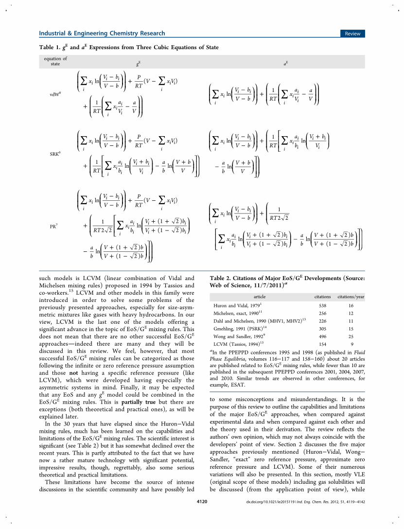
The gE and aE expressions from Soave−Redlich−Kwong(SRK)6 and Peng−Robinson (PR),7 the two cubic EoS whichare widely used today in practice, are shown in Table 1. For

comparison, the expressions from the van der Waals8 EoS arealso given. The expressions shown in Table 1 require no mixingrules as they are derived from the fundamental equations:

∑ ∑= φ − φ = γgRT

x xln ln lni

i ii

i i

E

(2a)

= −aRT

gRT

PVRT

E E E

(2b)

Moreover, the expressions of Table 1 are written in such a formso that the contributions related to excess entropy (SE), excessvolume (VE), and excess internal energy (UE) are identifiedsince:

= − + +gRT

SR

PVRT

URT

E E E E

(3a)

= − = − +aRT

gRT

PVRT

SR

URT

E E E E E

(3b)

Under some conditions, eq 1 can be solved with respect to theenergy parameter and a mixing rule can be derived. The mostknown reference pressures which have led to widely usedmixing rules are the infinite pressure and the zero pressure.The infinite pressure was the assumption used by Huron andVidal1 starting from eq 1a and 13 years later it was also used byWong and Sandler9 based on eq 1b. The zero referencepressure was introduced by Mollerup10 and Michelsen11,12 andleads to one exact formulation (under some assumptions) andto useful general but “approximate zero” reference pressuremixing rules like MHV1, MHV2 (modified Huron−Vidal firstand second order) by Dahl and Michelsen,13 and the PSRK(predictive SRK) model by Gmehling and co-workers.14 Therehave been also presented useful EoS/GE models which are notderived directly from eqs 1a or 1b. One of the most successful

Received: July 13, 2011Revised: February 16, 2012Accepted: February 16, 2012Published: February 16, 2012

Review

pubs.acs.org/IECR

© 2012 American Chemical Society 4119 dx.doi.org/10.1021/ie2015119 | Ind. Eng. Chem. Res. 2012, 51, 4119−4142

pubs.acs.org/IECR

such models is LCVM (linear combination of Vidal andMichelsen mixing rules) proposed in 1994 by Tassios andco-workers.15 LCVM and other models in this family wereintroduced in order to solve some problems of thepreviously presented approaches, especially for size-asym-metric mixtures like gases with heavy hydrocarbons. In ourview, LCVM is the last one of the models offering asignificant advance in the topic of EoS/GE mixing rules. Thisdoes not mean that there are no other successful EoS/GE

approachesindeed there are many and they will bediscussed in this review. We feel, however, that mostsuccessful EoS/GE mixing rules can be categorized as thosefollowing the infinite or zero reference pressure assumptionand those not having a specific reference pressure (likeLCVM), which were developed having especially theasymmetric systems in mind. Finally, it may be expectedthat any EoS and any gE model could be combined in theEoS/GE mixing rules. This is partially true but there areexceptions (both theoretical and practical ones), as will beexplained later.In the 30 years that have elapsed since the Huron−Vidal

mixing rules, much has been learned on the capabilities andlimitations of the EoS/GE mixing rules. The scientific interest issignificant (see Table 2) but it has somewhat declined over therecent years. This is partly attributed to the fact that we havenow a rather mature technology with significant potential,impressive results, though, regrettably, also some serioustheoretical and practical limitations.These limitations have become the source of intense

discussions in the scientific community and have possibly led

to some misconceptions and misunderstandings. It is thepurpose of this review to outline the capabilities and limitationsof the major EoS/GE approaches, when compared againstexperimental data and when compared against each other andthe theory used in their derivation. The review reflects theauthors’ own opinion, which may not always coincide with thedevelopers’ point of view. Section 2 discusses the five majorapproaches previously mentioned (Huron−Vidal, Wong−Sandler, “exact” zero reference pressure, approximate zeroreference pressure and LCVM). Some of their numerousvariations will also be presented. In this section, mostly VLE(original scope of these models) including gas solubilities willbe discussed (from the application point of view), while

Table 1. gE and aE Expressions from Three Cubic Equations of State

equation ofstate gE aE

vdW8

∑ ∑

∑

−−

+ −

+ −

⎛

⎝⎜⎜

⎛⎝⎜

⎞⎠⎟⎞

⎠⎟⎟

⎛

⎝⎜⎜

⎛

⎝⎜⎜

⎞

⎠⎟⎟⎞

⎠⎟⎟

xV bV b

PRT

V x V

RTx

aV

aV

ln ( )

1

ii

i i

ii i

ii

i

i

∑ ∑−−

+ −⎛

⎝⎜⎜

⎛⎝⎜

⎞⎠⎟⎞

⎠⎟⎟

⎛

⎝⎜⎜

⎛

⎝⎜⎜

⎞

⎠⎟⎟⎞

⎠⎟⎟x

V bV b RT

xaV

aV

ln1

ii

i i

ii

i

i

SRK6

∑ ∑

∑

−−

+ −

++

− +⎜ ⎟

⎛

⎝⎜⎜

⎛⎝⎜

⎞⎠⎟⎞

⎠⎟⎟

⎛

⎝⎜⎜

⎡

⎣⎢⎢

⎛⎝⎜

⎞⎠⎟

⎛⎝

⎞⎠⎤

⎦⎥⎥⎞

⎠⎟⎟

xV bV b

PRT

V x V

RTx

ab

V bV

ab

V bV

ln ( )

1ln ln

ii

i i

ii i

ii

i

i

i i

i

∑ ∑−−

++

− +⎜ ⎟

⎛

⎝⎜⎜

⎛⎝⎜

⎞⎠⎟⎞

⎠⎟⎟

⎛

⎝⎜⎜

⎡

⎣⎢⎢

⎛⎝⎜

⎞⎠⎟

⎛⎝

⎞⎠⎤

⎦⎥⎥⎞

⎠⎟⎟

xV bV b RT

xab

V bV

ab

V bV

ln1

ln

ln

ii

i i

ii

i

i

i i

i

PR7

∑ ∑

∑

−−

+ −

++ ++ −

− + ++ −

⎛

⎝⎜⎜

⎛⎝⎜

⎞⎠⎟⎞

⎠⎟⎟

⎛

⎝⎜⎜

⎡

⎣⎢⎢

⎛⎝⎜

⎞⎠⎟

⎛⎝⎜

⎞⎠⎟⎤

⎦⎥⎥⎞

⎠⎟⎟

xV bV b

PRT

V x V

RTx

ab

V bV b

ab

V bV b

ln ( )

12 2

ln(1 2 )(1 2 )

ln(1 2 )(1 2 )

ii

i i

ii i

ii

i

i

i i

i i

∑

∑

−−

+

+ ++ −

− + ++ −

⎛

⎝⎜⎜

⎛⎝⎜

⎞⎠⎟⎞

⎠⎟⎟

⎛

⎝⎜⎜

⎡

⎣⎢⎢

⎛⎝⎜

⎞⎠⎟

⎛⎝⎜

⎞⎠⎟⎤

⎦⎥⎥⎞

⎠⎟⎟

xV bV b RT

xab

V bV b

ab

V bV b

ln12 2

ln(1 2 )(1 2 )

ln(1 2 )(1 2 )

ii

i i

ii

i

i

i i

i i

Table 2. Citations of Major EoS/GE Developments (Source:Web of Science, 11/7/2011)a

article citations citations/year

Huron and Vidal, 19791 538 16

Michelsen, exact, 199011 256 12

Dahl and Michelsen, 1990 (MHV1, MHV2)13 226 11

Gmehling, 1991 (PSRK)14 305 15

Wong and Sandler, 19929 496 25

LCVM (Tassios, 1994)15 154 9aIn the PPEPPD conferences 1995 and 1998 (as published in FluidPhase Equilibria, volumes 116−117 and 158−160) about 20 articlesare published related to EoS/GE mixing rules, while fewer than 10 arepublished in the subsequent PPEPPD conferences 2001, 2004, 2007,and 2010. Similar trends are observed in other conferences, forexample, ESAT.

Industrial & Engineering Chemistry Research Review

dx.doi.org/10.1021/ie2015119 | Ind. Eng. Chem. Res. 2012, 51, 4119−41424120

other properties (LLE, solid−gas equilibria, thermal) will bebriefly considered in section 3, where a comparativediscussion and evaluation of all mixing rules will also bepresented. The review closes with the conclusions andassessment of the status of EoS/GE methodology, about 30years after its conception.

2. CAPABILITIES AND LIMITATIONS OF THE FIVEMAJOR EOS/GE APPROACHES

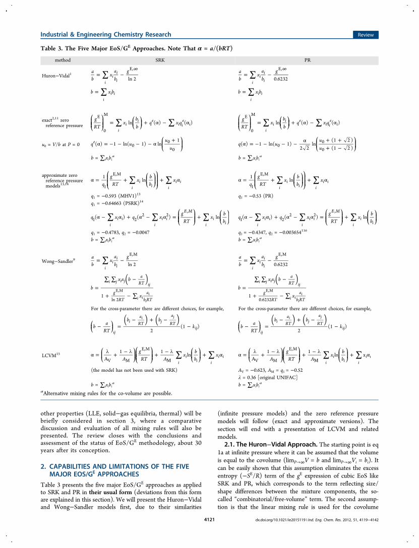
Table 3 presents the five major EoS/GE approaches as appliedto SRK and PR in their usual form (deviations from this formare explained in this section). We will present the Huron−Vidaland Wong−Sandler models first, due to their similarities

(infinite pressure models) and the zero reference pressuremodels will follow (exact and approximate versions). Thesection will end with a presentation of LCVM and relatedmodels.

2.1. The Huron−Vidal Approach. The starting point is eq1a at infinite pressure where it can be assumed that the volumeis equal to the covolume (limP→∞V = b and limP→∞Vi = bi). Itcan be easily shown that this assumption eliminates the excessentropy (−SE/R) term of the gE expression of cubic EoS likeSRK and PR, which corresponds to the term reflecting size/shape differences between the mixture components, the so-called “combinatorial/free-volume” term. The second assump-tion is that the linear mixing rule is used for the covolume

Table 3. The Five Major EoS/GE Approaches. Note That α = a/(bRT)

method SRK PR

Huron−Vidal1 ∑= −∞a

bx

ab

gln 2

ii

i

i

E,∑= −

∞ab

xab

g0.6232

ii

i

i

E,

∑=b x bi

i i ∑=b x bi

i i

exact2,11 zeroreference pressure ∑ ∑= + α − α

⎛⎝⎜⎜

⎞⎠⎟⎟

⎛⎝⎜

⎞⎠⎟

gRT

xbb

q x qln ( ) ( )i

ii e

i ie

iE

0

M

∑ ∑= + α − α⎛⎝⎜⎜

⎞⎠⎟⎟

⎛⎝⎜

⎞⎠⎟

gRT

xbb

q x qln ( ) ( )i

ii e

i ie

iE

0

M

u0 = V/b at P = 0 α = − − − − α+⎛

⎝⎜⎞⎠⎟q u

uu

( ) 1 ln( 1) ln1e

00

0α = − − − − α + +

+ −

⎛⎝⎜

⎞⎠⎟q u

uu

( ) 1 ln( 1)2 2

ln(1 2 )(1 2 )0

0

0

b = ∑ixibia b = ∑ixibi

a

approximate zeroreference pressuremodels13,14

∑ ∑α = + + α⎛

⎝⎜⎜

⎛⎝⎜

⎞⎠⎟⎞

⎠⎟⎟q

gRT

x bb

x1ln

ii

i ii i

1

E,M∑ ∑α = + + α

⎛

⎝⎜⎜

⎛⎝⎜

⎞⎠⎟⎞

⎠⎟⎟q

gRT

x bb

x1ln

ii

i ii i

1

E,M

q1 = −0.593 (MHV1)13 q1 = −0.53 (PR)q1 = −0.64663 (PSRK)14

∑ ∑ ∑α − α + α − α = +⎛⎝⎜⎜

⎞⎠⎟⎟

⎛⎝⎜

⎞⎠⎟q x q x

gRT

x bb

( ) ( ) lni

i ii

i iE M

ii

i1 2

2 2,

∑ ∑ ∑α − α + α − α = +⎛⎝⎜⎜

⎞⎠⎟⎟

⎛⎝⎜

⎞⎠⎟q x q x

gRT

x bb

( ) ( ) lni

i ii

i iE M

ii

i1 2

2 2,

q1 = −0.4783, q2 = −0.0047 q1 = −0.4347, q2 = −0.003654116


a

Wong−Sandler9 ∑= −ab

xab

gln 2

ii

i

i

E,M∑= −a

bx

ab

g0.6232

ii

i

i

E,M

=∑ ∑ −

+ − ∑

( )b

x x b

x1

i j i ja

RT ij

gRT i i

ab RTln 2

i

i

E,M =∑ ∑ −

+ − ∑

( )b

x x b

x1

i j i ja

RT ij

gRT i i

ab RT0.6232

i

i

E,M

For the cross-parameter there are different choices, for example, For the cross-parameter there are different choices, for example,

− =− + −

−⎜ ⎟⎛⎝

⎞⎠

( )( )b a

RT

b bk

2(1 )

ij

ia

RT ja

RTij

i j

− =− + −

−⎜ ⎟⎛⎝

⎞⎠

( )( )b a

RT

b bk

2(1 )

ij

ia

RT ja

RTij

i j

LCVM15 ∑ ∑α = λΑ

+ − λ + − λ + αΜ

⎛⎝⎜

⎞⎠⎟⎛⎝⎜⎜

⎞⎠⎟⎟

⎛⎝⎜

⎞⎠⎟A

gRT A

x bb

x1 1ln

ii

i ii i

V M

E,M∑ ∑α = λ

Α+ − λ + − λ + α

Μ

⎛⎝⎜

⎞⎠⎟⎛⎝⎜⎜

⎞⎠⎟⎟

⎛⎝⎜

⎞⎠⎟A

gRT A

x bb

1 1ln x

ii

i ii i

V M

E,M

(the model has not been used with SRK) AV = −0.623, AM = q1 = −0.52λ = 0.36 [original UNIFAC]


a

aAlternative mixing rules for the co-volume are possible.



(b = ∑ixibi), see Table 3, which eliminates the excess volumeterm at infinite pressure. Thus at infinite pressure:

∑

∑

= = = −

= ε − ε ε =

=

=

=

∞ ∞ ⎛

⎝⎜⎜

⎛

⎝⎜⎜

⎞

⎠⎟⎟⎞

⎠⎟⎟

⎛

⎝⎜⎜

⎞

⎠⎟⎟

gRT

URT

gRT

ART

xab

ab

ART

x ab

A

A

A

1 (vdW, van Laar)

ln 2 (SRK)

0.623 (PR)

ii

i

i

ii i

E,EoS, P E, E,resV

V

V

V

V (4)

Equation 4, also shown in Table 3, is the Huron−Vidalmixing rule.1 It is clear that the linear mixing rule for thecovolume is used in its derivation and no other mixing rules forthe covolume can be used in order to arrive to eq 4 when eq 1ais the starting point for the derivation.Another important remark is that, in general, gE,EoS,∞P ≠

gE,EoS,low,P, thus the existing parameter tables from activitycoefficient models which are obtained from low pressure datacannot be used in eq 4.It is also quite interesting to note that since at infinite

pressure SE = VE = 0 and gE= UE then the gE,EoS,∞P is essen-tially an ”energetic” or ”residual” (in the activity coefficientterminology) excess Gibbs energy contribution, and only suchactivity coefficient models should be used in connection withthe Huron−Vidal approach. Examples of such models areNRTL and the residual part of UNIQUAC or UNIFAC.Indeed, Huron and Vidal1,26 combined SRK with NRTL and

they presented excellent correlation results for the VLE ofacetone/water, methanol/CO2, methanol/propane, and othercomplex mixtures. The performance of SRK with the Huron−Vidal mixing rules is better than when SRK is used with thevan der Waals one fluid mixing rules (a = ∑i = 1

n ∑j = 1n xixjaij

b = ∑i = 1n ∑j = 1

n xixjbij). Good predictions are also obtained formulticomponent VLE.It should be noted that Huron and Vidal used an NRTL

version which, under certain assumptions for the parametervalues, can result in the vdW1f mixing rules for nonpolarcompounds. In this way, the SRK EoS can be used for mixturesof polar and nonpolar compounds, using the classicalinteraction parameters in cross a12 or the Huron−Vidalparameters. This permits reusing the interaction parametertables for kij (correction in the geometric mean rule for thecross energy parameter) available for SRK for mixtures withnonpolar compounds.The Huron−Vidal mixing rule has been widely used both in

academia and industry. It has been shown16−20 (in its SRK/NRTL formulation) to be an excellent correlation tool even forhighly complex VLE, LLE, and VLLE for a variety of mixturesincluding those containing water, alcohols, or glycols andhydrocarbons and for both binary and multicomponentmixtures. Parameters obtained from correlating binary datacan be used to predict phase equilibria for multicomponentsystems (see also the discussion in section 3).Feroiu, Geana, and co-workers21−24 have shown that SRK/

Huron−Vidal coupled with the residual term of UNIQUACand parameters obtained from infinite dilution data cancorrelate/predict CO2-alcohols VLE and VLLE over extensivetemperature ranges. It should be emphasized that for obtaininggood results over broad temperature ranges, (linearly)

temperature dependent interaction parameters are needed inthe local composition model. Note that, in agreement to theprevious discussion, the combinatorial term of UNIQUAC isdropped.Vidal himself in a series of publications25−27 proposed

combining the Huron−Vidal mixing rule in SRK or PR usingthe residual term of UNIQUAC or UNIFAC, in the latter casefor developing a predictive model. Of course, in both cases newinteraction parameters (molecular or group ones) should bedetermined based on experimental data. Later, Soave and co-workers28−34 continued this work proposing an SRK/Huron−Vidal model with the residual term of UNIFAC and applied thederived model (UNIFEST) with success to some polarmixtures containing ethers, alcohols, ketones, esters, andalkanes or light gases. More work was in progress28,29 but tothe knowledge of the authors this group contribution SRK/Huron−Vidal parameter table has not been completed (see,however, the discussion in section 3 and ref 98). In the first ofthese publications28 Soave illustrated (Figure 3 of ref 28) thatthe combinatorial term of the external model (UNIFAC)should be dropped as “calculations have shown that it causes anexcessive decrease of volatility which cannot be compensated inmixtures of light and heavy hydrocarbons”.28 The test system wasethane/octane at 25 °C. Soave29 also mentioned that “thecombinatorial term produced over-specif ied coef f icient values”.29

We believe that these conclusions from Soave are correct andconsistent with the derivation of the Huron−Vidal mixing rule,see eq 4, since the excess Gibbs energy at infinite pressure fromthe EoS only corresponds to its “energetic” or “residual” part.Thus, in the case of the Huron−Vidal mixing rule, eq 1a impliesequating the energetic gE from the EoS (right-hand side of eq 4)and from an explicit activity coefficient model.We will further elucidate this point by looking at the activity

coefficient equation derived from SRK using the Huron−Vidaland classical mixing rules. Following the discussion byKontogeorgis and co-workers16,35,37 and Sacomani andBrignole36 we will analyze the Huron−Vidal mixing rule bylooking at the activity coefficient equation, which unlike the gE

expression, depends on the mixing rule. To simplify things, welimit our discussion to infinite dilution conditions, zero valuesof the interaction parameters and binary systems. Under theseconditions, and using the linear mixing rule for the covolumeparameter, the expressions for the activity coefficient are forSRK with the various mixing rules given in eqs 5a−5d (notethat ∞ indicates infinite dilution here).

SRK with vdW1f mixing rules:

γ = γ + γ

=−−

+ −−−

++

++

−+

+ − +

∞ −

⎛⎝⎜

⎞⎠⎟

⎛⎝⎜

⎞⎠⎟

⎛⎝⎜

⎞⎠⎟

⎛⎝⎜

⎞⎠⎟

⎛⎝⎜⎜

⎞⎠⎟⎟

⎡⎣⎢

⎤⎦⎥

⎛⎝⎜

⎞⎠⎟

V bV b

V bV b

ab RT

ab RT

V b V b

V b V

bRT

ab

ab

bV

ln ln ln

ln 1

ln1

1

ln 1

bV

bV

1 1comb FV

1res

1 1

2 2

1 1

2 2

1

1

2

2

1 2 2 1

22

2 2

1 2

2

1

1

22

2

1

1

2

2

(5a)

SRK using the simplified mixing rule a/b = ∑ixiai/bi(this form of the equation corresponds to using only



the combinatorial/free-volume contribution of the cubicEoS):

γ = γ =−−

+ −−−

++

++

−+

∞ − ⎛⎝⎜

⎞⎠⎟

⎛⎝⎜

⎞⎠⎟

⎛⎝⎜

⎞⎠⎟

⎛⎝⎜

⎞⎠⎟

⎛⎝⎜⎜

⎞⎠⎟⎟

V bV b

V bV b

ab RT

ab RT

V b V b

V b V

ln ln ln 1

ln1

1

bV

bV

1 1comb FV 1 1

2 2

1 1

2 2

1

1

2

2

1 2 2 1

22

2 2

1

1

2

2 (5b)

SRK using the Huron−Vidal mixing rule (using an externalactivity coefficient without or with an explicit combinatorialterm):

γ = γ + γ

=−−

+ −−−

++

+

+−

++ − +

γ

∞ −

⎛⎝⎜

⎞⎠⎟

⎛⎝⎜

⎞⎠⎟

⎛⎝⎜

⎞⎠⎟

⎛⎝⎜

⎞⎠⎟

⎛⎝⎜⎜

⎞⎠⎟⎟

⎛⎝⎜

⎞⎠⎟

⎛⎝⎜

⎞⎠⎟

V bV b

V bV b

ab RT

ab RT

V b V b

V b V AV b

V

ln ln ln

ln 1 ln1

1

1ln ln

bV

bV

1 1comb FV

1res

1 1

2 2

1 1

2 2

1

1

2

2

1 2 2 1

22

2 2 V

2 2

21res,M

1

1

2

2

(5c)

γ = γ + γ

=−−

+ −−−

+

+

++

−+

+ − +γ + γ

∞ −

⎛⎝⎜

⎞⎠⎟

⎛⎝⎜

⎞⎠⎟

⎛⎝⎜

⎞⎠⎟

⎛⎝⎜

⎞⎠⎟

⎛⎝⎜⎜

⎞⎠⎟⎟

⎛⎝⎜

⎞⎠⎟

⎛⎝⎜

⎞⎠⎟

V bV b

V bV b

ab RT

ab RT

V b V b

V b V

AV b

V

ln ln ln

ln 1

ln1

1

1ln (ln ln )

bV

bV

V

comb M

1 1comb FV

1res

1 1

2 2

1 1

2 2

1

1

2

2

1 2 2 1

22

2 2

2 2

21

,1res,M

1

1

2

2

(5d)

where M is the external activity coefficient model such asNRTL. We use the symbol “res,M” to emphasize that onlythe residual term of an activity coefficient model or a purelyenergetic model should be used in the Huron−Vidal model.Nevertheless, if an activity coefficient model having bothcombinatorial and residual terms is used, then eq 5dapplies.By comparing eqs 5a−5c we can see that SRK with the

Huron−Vidal mixing rule essentially modifies only the residualterm of the equation of state (compared to the classical vdW1fmixing rule). This residual part is, for the vdW1f mixing rules,represented by the last bracketed term in eq 5a, which is aregular solution type term. In the case of SRK/Huron−Vidalthis residual term is given by a local composition model (lastterm in eq 5c). The SRK EoS with the Huron−Vidal mixingrule has the same combinatorial-free volume term as SRK withthe vdW1f mixing rules. It is thus clear that the performanceof SRK/Huron−Vidal EoS coupled with NRTL cannot beidentical to that of NRTL, especially for size-asymmetricsystems, even at low pressures. This is because the EoS/GE

model contains a combinatorial term, while the explicit gE

model (NRTL) does not.

Following previous investigations16,35−37 we can claim thatthe first term of eqs 5a and 5c (and the full eq 5b) is thecombinatorial-free volume or size term of the EoS. It representsindeed the term that disappears at infinite pressure (if we setV = b and Vi = bi), exactly as the SE and VE terms vanish atinfinite pressure. The regular solution terms in eq 5a or γres,M ineq 5c which do not disappear at infinite pressure are the energyterms of the EoS. Having said that, how successfully do thewell-known cubic EoS like SRK or PR represent nearlyathermal mixtures with large size differences between thecomponents which could provide a test for the combinatorial/free-volume term of cubic EoS ? Mixtures of alkanes offer anexcellent such test as these are considered nearly athermal and,for example, ln γres,M = 0 from UNIFAC for such systems. Theresults shown in refs 16 and 35−37 as well as some typical resultsgiven in Table 4 and Figure 1 illustrate that the combinatorial-free

volume term of cubic EoS does provide qualitatively and in manycases even quantitatively correct results.The results in Table 4 and Figure 1 are based on the Peng−

Robinson equation of state for which the equations are similarto eqs 5a−5c:PR with vdW1f mixing rules:

γ =−−

+ −−−

+

+−

+ −

+ −

∞ ⎛⎝⎜

⎞⎠⎟

⎛⎝⎜

⎞⎠⎟

⎛⎝⎜⎜

⎞⎠⎟⎟

⎡⎣⎢

⎤⎦⎥

V bV b

V bV b

ab RT

f b Vf b V

ab RT

V b V b

V b V b

bRT

ab

ab

f b V

ln ln 12 2

ln( , )( , ) 2

2 2ln ( , )

11 1

2 2

1 1

2 2

1

1

1 1

2 2

2

2

1 2 2 1

22

2 2 22

1 2

2

1

1

2

2 2(6a)

Table 4. Percentage Absolute Deviation betweenExperimental and Calculated Activity Coefficients at InfiniteDilution for n-Butane and n-Heptane in Various AlkanesUsing the PR EoS and Various Mixing Rules. ForComparison the Deviations with Original and ModifiedUNIFAC Combinatorials5,112 Are Also Given

alkane or.UNIFAC mod.UNIFAC

PR−vdW1f,eq 6a(kij = 0)

PR-a/bor

Vidal,eqs 6bor 6c

PR−Vidal,eq 6d (usingor.UNIFACin the external

model)

n-Butane

20 39 16 27 0.6 46

22 41 17 32 1.1 50

24 40 13 44 2.0 51

28 43 13 54 2.5 58

32 45 11 68 5.3 63

36 46 10 83 9.3 67

average 42 13 51 3.5 56n-Heptane

20 21 6.8 15 5.3 31

22 25 9.1 18 11.1 38

24 24 5.2 29 9.3 40

28 26 3.0 45 11.7 47

32 28 1.9 63 15.6 53

36 30 0.2 85 19.3 58

average 26 4.4 43 12 45



PR using the simplified mixing rule a/b = ∑ixiai/bi:

γ =−−

+ −−−

+

+−

+ −

∞ ⎛⎝⎜

⎞⎠⎟

⎛⎝⎜

⎞⎠⎟

⎛⎝⎜⎜

⎞⎠⎟⎟

V bV b

V bV b

ab RT

f b Vf b V

ab RT

V b V b

V b V b

ln ln 12 2

ln( , )( , ) 2

11 1

2 2

1 1

2 2

1

1

1 1

2 2

2

2

1 2 2 1

22

2 2 22

(6b)

PR using the Huron−Vidal mixing rule (using an externalactivity coefficient without or with an explicit combinatorialterm):

γ =−−

+ −−−

+

+−

+ −

+ − γ

∞ ⎛⎝⎜

⎞⎠⎟

⎛⎝⎜

⎞⎠⎟

⎛⎝⎜⎜

⎞⎠⎟⎟

⎛⎝⎜

⎞⎠⎟⎛⎝⎜

⎞⎠⎟

V bV b

V bV b

ab RT

f b Vf b V

ab RT

V b V b

V b V b

Af b V

ln ln 12 2

ln( , )( , ) 2

1 ln ( , )2 2

lnV

11 1

2 2

1 1

2 2

1

1

1 1

2 2

2

2

1 2 2 1

22

2 2 22

2 21res,M

(6c)

γ =−−

+ −−−

+

+−

+ −

+ − γ + γ

∞ ⎛⎝⎜

⎞⎠⎟

⎛⎝⎜

⎞⎠⎟

⎛⎝⎜⎜

⎞⎠⎟⎟

⎛⎝⎜

⎞⎠⎟⎛⎝⎜

⎞⎠⎟

V bV b

V bV b

ab RT

f b Vf b V

ab RT

V b V b

V b V b

Af b V

ln ln 12 2

ln( , )( , ) 2

1 ln ( , )2 2

(ln ln )V

11 1

2 2

1 1

2 2

1

1

1 1

2 2

2

2

1 2 2 1

22

2 2 22

2 21comb,M

1res,M

(6d)

In all the above cases:

=+ ++ −

⎡⎣⎢

⎤⎦⎥f b V

V bV b

( , )(1 2 )(1 2 )i i

i i

i i

and the function f(b2,V2) is the same as f(b1,V1), with change ofsubscripts.We note that the results with the cubic EoS combinatorial/

free-volume activity coefficient (or simply the a/b mixing rule)

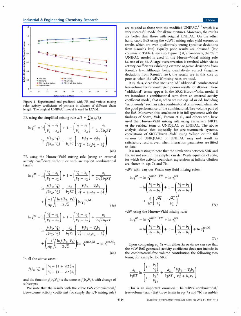
are as good as those with the modified UNIFAC,112 which is avery successful model for alkane mixtures. Moreover, the resultsare better than those with original UNIFAC. On the otherhand, cubic EoS using the vdW1f mixing rules yield erroneousresults which are even qualitatively wrong (positive deviationsfrom Raoult’s law). Equally poor results are obtained (lastcolumns in Table 4; see also Figure 1) if, erroneously, the “full”UNIFAC model is used in the Huron−Vidal mixing rulei.e. use of eq 6d. A large overcorrection is resulted which yieldsactivity coefficients exhibiting extreme negative deviations fromRaoult’s law. Although being qualitatively correct (negativedeviations from Raoult’s law), the results are in this case aspoor as when the vdW1f mixing rules are used.It is, thus, clear that inclusion of “additional” combinatorial

free-volume terms would yield poorer results for alkanes. These“additional” terms appear in the SRK/Huron−Vidal model ifwe introduce a combinatorial term from an external activitycoefficient model, that is, when we use eqs 5d or 6d. Including“erroneously” such an extra combinatorial term would eliminatethe good performance of the combinatorial/free-volume part ofthe EoS. Moreover, this conclusion is in full agreement with thefindings of Soave, Vidal, Feoiou et al., and others who haveused the Huron−Vidal mixing rule using exclusively NRTLor the residual term of UNIQUAC or UNIFAC. The aboveanalysis shows that especially for size-asymmetric systems,correlations of SRK/Huron−Vidal using Wilson or the fullversion of UNIQUAC or UNIFAC may not result insatisfactory results, even when interaction parameters are fittedto data.It is interesting to note that the similarities between SRK and

PR are not seen in the simpler van der Waals equation of state,for which the activity coefficient expressions at infinite dilutionare shown in eqs 7a and 7b.

vdW with van der Waals one fluid mixing rules:

γ = γ + γ

=−−

+ −−−

+ −

∞ −

⎛⎝⎜

⎞⎠⎟

⎛⎝⎜

⎞⎠⎟

⎛⎝⎜

⎞⎠⎟

V bV b

V bV b

VRT

aV

aV

ln ln ln

ln 1

1 1comb FV

1res

1 1

2 2

1 1

2 2

1 1

1

2

2

2

(7a)

vdW using the Huron−Vidal mixing rule:

γ = γ + γ

=−−

+ −−−

+ γ

∞ −

⎛⎝⎜

⎞⎠⎟

⎛⎝⎜

⎞⎠⎟

V bV b

V bV b

ln ln ln

ln 1 ln

1 1comb FV

1res

1 1

2 2

1 1

2 21res,M

(7b)

Upon comparing eq 7a with either 5a or 6a we can see thatthe vdW EoS generated activity coefficient does not include inthe combinatorial-free volume contribution the following twoterms, for example, for SRK

+

++

−+

⎛⎝⎜

⎞⎠⎟

⎛⎝⎜

⎞⎠⎟

⎛⎝⎜⎜

⎞⎠⎟⎟a

b RTa

b RTV b V b

V b Vln

1

1

bV

bV

1

1

2

2

1 2 2 1

22

2 2

1

1

2

2

This is an important omission. The vdW’s combinatorial/free-volume term (first three terms in eqs 7a and 7b) resembles

Figure 1. Experimental and predicted with PR and various mixingrules activity coefficients of pentane in alkanes of different chainlength. The original UNIFAC5 model is used in LCVM.



http://pubs.acs.org/action/showImage?doi=10.1021/ie2015119&iName=master.img-000.jpg&w=239&h=181

indeed activity coefficient models suitable for polymersolutions, like Flory−Huggins113 or Entropic-FV.114 However,using EoS-generated volumes, this term alone results to activitycoefficients only slightly below unity for alkane mixtures. Theseactivity coefficient values are in the right trend qualitatively inagreement to the experimental data (negative deviations fromRaoult’s law) but quantitatively they deviate significantly fromthe experimental values, as shown by Kontogeorgis et al.38

In conclusion, the Huron−Vidal mixing rule is an excellentcorrelative tool for low and high pressure VLE of complexsystems and it is important to employ an energetic activitycoefficient model in the mixing rule, for example, NRTL. Theparameters must be refitted to data using the EoS and themixing rule meaning that existing parameters cannot be useddue to the infinite pressure assumption in the mixing rulederivation. There is another significant “double limitation”. Thederivation of eq 4 is based on the linear mixing rule for thecovolume. This is indeed the most widely used mixing rule forthe covolume in cubic EoS, and often good results are obtained.Moreover, using this combining rule, the combinatorial/free-volume contribution to the activity coefficient has the form ofeqs 5 or 6, which results to satisfactory but not perfect results(for nearly athermal mixtures). The mixing rule for thecovolume affects the liquid-phase properties especially for size-asymmetric systems and as shown by Kontogeorgis et al.38 asingle interaction parameter [bij = ((bi + bj)/2))(1 − lij)] canimprove dramatically the results of cubic EoS (see also later,after eq 43). The lij parameter can effectively modify thecombinatorial/free-volume contribution in the right directionand even adjust accordingly the energetic term of EoS, as themixing rule for the covolume appears in all terms of cubic EoS-generated activity coefficients. Kontogeorgis et al.38 showed forexample that by using a single lij equal to about 0.02 accurateresults are obtained with the PR EoS for mixtures of ethanewith alkanes varying from decane to C44. The same is notpossible with a single kij interaction parameter. However,the derivation of the Huron−Vidal mixing rule restricts thecubic EoS of the possibility of employing this extra degree offreedom, as a linear mixing rule for the covolume is imper-ative in its derivation. Moreover, the SRK using Huron−Vidal mixing rule violates the imposed by statistical thermo-dynamics quadratic composition dependency of the secondvirial coefficient:

∑ ∑=B x x Bi j

i j ij(8)

The second virial coefficient from cubic EoS like vdW, SRK,and PR is given as

= −B ba

RT (9)

Even though cubic EoS do not give good second virialcoefficients for pure compounds, it might be of interest tosatisfy the theoretically correct limit of eq 8. Vidal1,39 wasaware of this limitation but he and others have stated that it isdifficult to establish what importance should be attributed tothis limitation and what is to gain by satisfying eq 8 for practicalapplications. Vidal39 writes: “we have never observed practicalproblems attributable to this defect”. Note that the classicalvdW1f mixing rules do satisfy this theoretical limit. Wong andSandler proposed in 19929 in a truly novel way a modificationof the Huron−Vidal mixing rule which addresses several of its

limitations, permitting the use of existing interaction parameterdatabases, utilization of the extra degree of freedom bymodifying the mixing rule for the covolume parameter and sat-isfaction of eq 8. Some other issues have been raised however.We discuss the Wong−Sandler mixing rule next.

2.2. The Wong−Sandler Mixing Rule. The Wong−Sandler mixing rule is, like Huron−Vidal, also based on theinfinite reference pressure but with significant modificationscompared to that in Huron−Vidal:

i First of all, the starting point is not eq 1a but eq 1b(at infinite pressure). Thus, by equating the excessHelmholtz energies, the excess volume term is eliminated(see eq 3b and Table 1).

ii Wong and Sandler assumed that the following isapproximately true:

≈ ≈ ≈∞a a a gmodelE

PE

lowPE

lowPE

(10)

The middle equality of the excess Helmholtz energyat infinite pressure with the excess Gibbs energy atlow pressure is based in the empirical finding40 of the relativeinsensitivity of the excess Helmholtz energy with pressure,whereas it is well-known that gE is highly dependent onpressure. Wong et al.42 justified also numerically this equalityfor the system methanol/benzene.

iii Having now the possibility for an additional degree offreedom, Wong and Sandler9 choose to satisfy eq 8, thus:

∑ ∑− = −⎜ ⎟ ⎜ ⎟⎛⎝

⎞⎠

⎛⎝

⎞⎠b

aRT

x x ba

RTi j

i jij (11)

The Wong−Sandler mixing rule is derived from statementsi−iii and eq 1b as follows. First, from statements i and ii,expressions identical to Huron−Vidal mixing rule are obtained(see also Table 3). In the case of Peng−Robinson we get

∑ ∑= − = −∞a

bx

ab

ax

ab

g0.6232 0.6232

ii

i

i

E

ii

i

i

, E,M

(12)

Substituting eq 12 in eq 11 we get, for the PR EoS,

=∑ ∑ −

+ − ∑

( )b

x x b

x1

i j i ja

RT ij

gRT i i

ab RT0.6232

i

i

E,M

(13)

similar to SRK (see Table 3). So, the covolume parameter canbe calculated from eq 13, and then the mixing rule for theenergy parameter can be obtained from eq 12. In this way anexcess Gibbs energy model with existing low-pressure obtainedparameters gE,M can be in principle used. The Wong−Sandlermixing rule is defined by eqs 12 and 13 together with anexpression for the cross virial coefficient. This last point is not atrivial issue and indeed, as explained later, the cross virialcoefficient term plays a major role in the Wong−Sandlermodel. This is the case because of the uncertainty about whichcombining rule should be used for the cross virial coefficient.Moreover, Wong and Sandler9 (and most subsequentinvestigators) have employed an interaction parameter kij in



the model. The following choices for the cross virial coefficienthave been reported:

− =− + −

−⎜ ⎟⎛⎝

⎞⎠

( )( )b a

RT

b bk

2(1 )

ij

ia

RT ja

RTij

i j

(14a)

− =+

− −⎜ ⎟⎛⎝

⎞⎠b

aRT

b b a a

RTk

2(1 )

ij

i j i jij

(14b)

(The possibility of using kij = 0 in eq 14a results in a linearmixing rule for the second virial coefficient, but this possibilityhas not been tested for the Wong−Sandler mixing rule).Wong and Sandler9 determined kij from experimental VLE

data at one temperature and x = 0.5, while Orbey et al.41,43

fitted kij to UNIFAC-obtained infinite dilution activitycoefficients at x = 0.5, thus rendering the model fully predictive.It is evident from the aforementioned discussion that, despite

the apparent similarities, there are fundamental differencesbetween the Huron−Vidal and Wong−Sandler approaches.Great successes have been reported for the Wong−Sandler

mixing rule. For example, Wong et al.42 using van Laar as the gE

model with parameters estimated from low pressure data andkij = 0.326 predicted VLE for 2-propanol/water in the range 150−275 °C and up to 100 bar with excellent results. Similar verysatisfactory results were obtained for acetone/pentane, ethanol/water, and other systems, using either NRTL or van Laar as theactivity coefficient model incorporated. These examples, furtherverified and elaborated in subsequent publications, illustratethe key success of the Wong−Sandler mixing rule, namely topredict VLE using existing low pressure parameters fromactivity coefficient models over very extensive temperature andpressure ranges, thus extrapolating successfully far beyond gE

models alone could ever do on their own! Successful resultshave been obtained also for ternary and multicomponent VLE(and in some cases also VLLE), using binary system generatedparameters. This great success made the Wong−Sandler mixingrules the object of many investigations from numerousresearchers who applied the methodology also to liquid−liquidequilibria, excess enthalpies, solid−gas equilibria, even surfac-tants and polymers. Some of these applications are discussed insection 3.Following the discussion with the Huron−Vidal mixing rule,

the use of the “energetic” van Laar and NRTL models isconsistent with the infinite pressure derivation of the model (asSE = 0 in the model development). Still, the Wong−Sandlerrule has been used even with UNIQUAC and UNIFACwhich contain an external combinatorial term. This may be thecause of problems for size-asymmetric systems, as discussedbelow. Indeed, despite the significant success, there is a well-documented criticism regarding the Wong−Sandler mixingrules which mostly lies in the following four directions:(1) Even if we do not consider the kij of eq 14 as an

additional adjustable parameter but as a parameter that canbe obtained from the incorporated gE model, there is anuncertainty on how this parameter should be estimated, onwhich combining rule should be preferred for the cross secondvirial coefficient (eqs 14a or 14b or other) and on what exactlykij represents in the model (see also point 4 later). Can kij beestimated in a reliable way from cross second virial coefficientdata?(2) Equation 13 introduces a temperature dependent

covolume parameter. Such temperature-dependent covolumes

are for good reasons avoided in cubic EoS, as discussed byMichelsen and Mollerup44 and Satyro and Trebble.45,46 This isbecause they may result in negative heat capacities at certainhigh pressure conditions. Thus, can the fulfillment of onecorrect physical behavior (eq 8) lead to unphysical behavior foranother property?(3) The good extrapolation capabilities of Wong−Sandler

mixing rules may not necessarily be associated with thereproduction of the correct composition dependency of themixture second virial coefficient. As Michelsen and Heide-mann47 showed, the PR/Wong−Sandler model results to ratherlarge excess enthalpies which are closer to the experimental datacompared to the values produced by the incorporated gE modelof the mixing rule. Can the extrapolation success of Wong−Sandler mixing rules be, as Heidemann,48 writes “derived fromthis fortunate cancellation of errors?” We should point out,however, that Michelsen and Heidemann used the Wilsonmodel in their analysis of the Wong−Sandler mixing rules. Thisis a gE model with a combinatorial term (Flory−Huggins) andshould not be preferred when an infinite reference pressuremodel is used. Their analysis would have been more convincingif, for example, the NRTL model was used instead.(4) Coutsikos et al.49 published a systematic investigation of

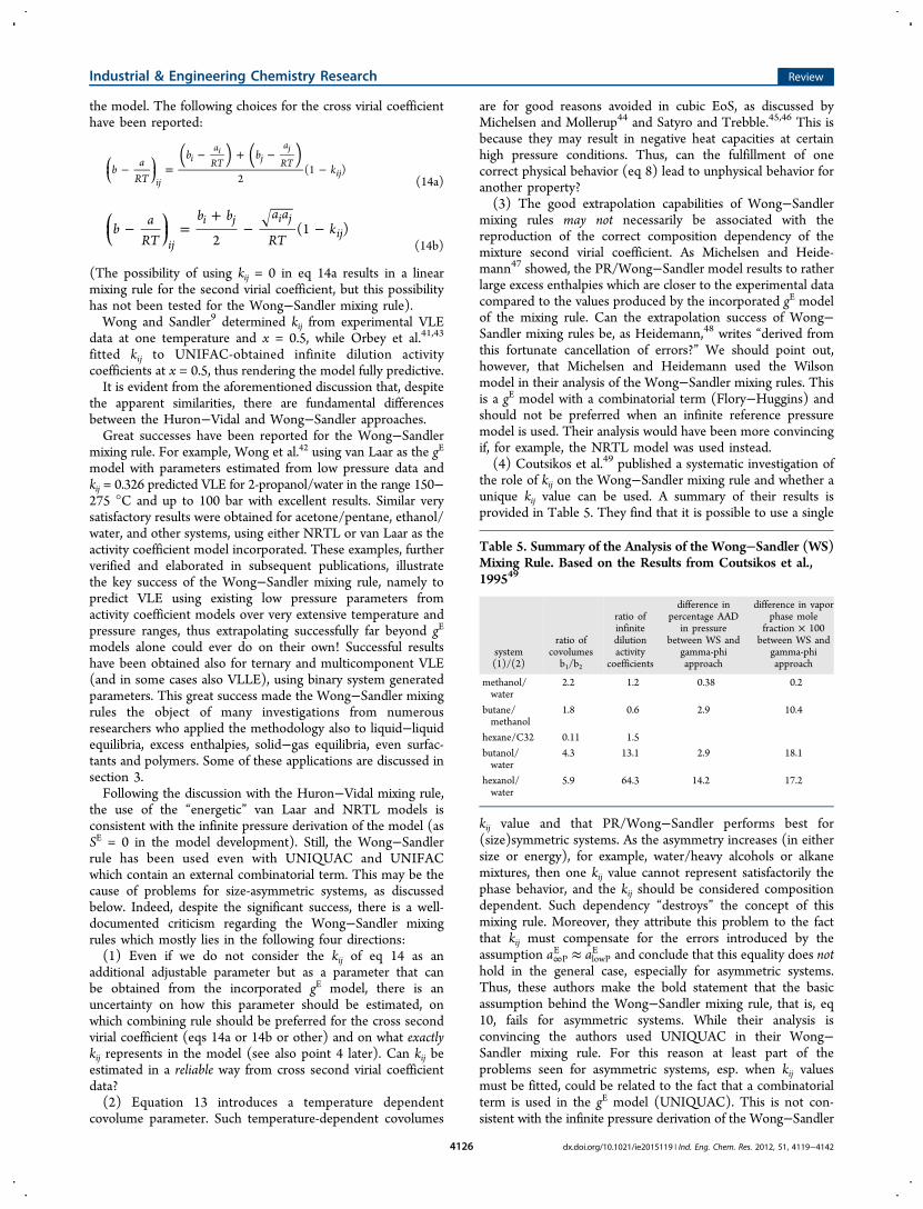
the role of kij on the Wong−Sandler mixing rule and whether aunique kij value can be used. A summary of their results isprovided in Table 5. They find that it is possible to use a single

kij value and that PR/Wong−Sandler performs best for(size)symmetric systems. As the asymmetry increases (in eithersize or energy), for example, water/heavy alcohols or alkanemixtures, then one kij value cannot represent satisfactorily thephase behavior, and the kij should be considered compositiondependent. Such dependency “destroys” the concept of thismixing rule. Moreover, they attribute this problem to the factthat kij must compensate for the errors introduced by theassumption a∞P

E ≈ alowPE and conclude that this equality does not

hold in the general case, especially for asymmetric systems.Thus, these authors make the bold statement that the basicassumption behind the Wong−Sandler mixing rule, that is, eq10, fails for asymmetric systems. While their analysis isconvincing the authors used UNIQUAC in their Wong−Sandler mixing rule. For this reason at least part of theproblems seen for asymmetric systems, esp. when kij valuesmust be fitted, could be related to the fact that a combinatorialterm is used in the gE model (UNIQUAC). This is not con-sistent with the infinite pressure derivation of the Wong−Sandler

Table 5. Summary of the Analysis of the Wong−Sandler (WS)Mixing Rule. Based on the Results from Coutsikos et al.,199549

system(1)/(2)

ratio ofcovolumesb1/b2

ratio ofinfinitedilutionactivity

coefficients

difference inpercentage AAD

in pressurebetween WS and

gamma-phiapproach

difference in vaporphase mole

fraction × 100between WS and

gamma-phiapproach

methanol/water

2.2 1.2 0.38 0.2

butane/methanol

1.8 0.6 2.9 10.4

hexane/C32 0.11 1.5

butanol/water

4.3 13.1 2.9 18.1

hexanol/water

5.9 64.3 14.2 17.2



mixing rule. Again, as in point 3, the analysis would have beenmore convincing if the NRTL or van Laar models were usedinstead.Finally, we should mention a practical problem of the

Wong−Sandler mixing rule. As with Huron−Vidal, and theother models discussed later, parameters for gas-containingsystems should be fitted separately in connection with thesemodels. This is because such parameters are not available inactivity coefficient models like NRTL and UNIFAC. Wong−Sandler rules have found so far limited applicability to gas-containing systems and extensive gas-containing tables are notavailable. Furthermore, the predictive approach of obtainingthe kij-parameters (using UNIFAC) is not applicable to gas-containing systems.2.3. The “Exact” Zero Reference Pressure Mixing Rule.

The idea behind the use of the Wong−Sandler mixing rule wasto use an external excess Gibbs energy model, gE,M, with existingparameters obtained from low pressure phase equilibrium data.An alternative approach to using eq 1b as a starting point theway Wong and Sandler did is to start with eq 1a and use a zeroreference pressure. This would always ensure reproduction ofthe incorporated gE model when a mathematical solution can beobtained for the energy parameter. The zero reference pressuremodels appeared in early 90s, chronologically prior to theWong−Sandler ones. The idea was put forward by Mollerup10

and Heidemann and Kokal50 but the mathematical problemwas, essentially, solved in a tractable way by Michelsen,11,12

who in 1990 presented the so-called “exact” model, shown inTable 3. This is an exact zero reference pressure mixing rule,ensuring full reproduction of the gE model incorporated.Unfortunately, the mixing rule is implicit with respect to theenergy parameter. Moreover, the mixing rule is not alwaysobtainable, but only when a liquid solution is available at zeropressure, that is, for values above the limiting values shownin Table 3. This can be easily understood as illustrated herefor SRK which at zero pressure and reduced variables (α =a/(bRT) and u0= V/b at P = 0) is written as

−− α

+=

u u u1

1 ( 1)0

0 0 0 (15)

The liquid volume solution at zero reference pressure is

= α − − α − α +u

( 1) 6 120

2

(16)

but evidently it exists only for αlim > 3 + 2√2 (Table 3 givesthe PR limiting value).When the liquid volume at zero pressure does exist, then the

fugacity coefficient from SRK,

φ =

= − − + − − +⎜ ⎟⎡⎣⎢

⎤⎦⎥

⎛⎝

⎞⎠

fP

P V bRT

PVRT

abRT

V bV

ln ln

ln( )

1 ln

(17a)

can be equivalently written as

− = α

= − − − − α+⎛

⎝⎜⎞⎠⎟

f

Pb q

uu

u

ln ln ( )

1 ln( 1) ln1

e0

00

0 (17b)

Then, from the equation

∑ ∑= φ − φ = −gRT

xf

RTx

f

RTln ln ln ln

ii i

ii

iE0 0,

(18)

and using eq 1a, the expression for the mixing rule is obtained:

∑ ∑= + α − α⎛⎝⎜⎜

⎞⎠⎟⎟

⎛⎝⎜

⎞⎠⎟

gRT

xbb

q x qln ( ) ( )i

ii e

i ie

iE

0

M

(19)

Michelsen12 showed that SRK coupled with Wilson and eq19 provided good results ensuring full reproduction of theWilson results at low pressures.It must be appreciated that eq 19:

• is mathematically correct at zero pressure withoutassumptions (other than the need for a liquid volumeat zero pressure)

• ensures full reproduction of the gE from the externalactivity coefficient model at zero pressure. Any gE modelcan be used including models with or withoutcombinatorial terms like Wilson, UNIQUAC or NRTL

• can be used with any low pressure activity coefficientmodels with existing interaction parameters obtainedfrom low pressure VLE or other data, for example, theparameters available in the Dechema or UNIFAC tablescan be used

• does not involve any assumption for the mixing rule forthe covolume parameter; linear, quadratic, or othermixing rules for the covolume parameter can be used

There are limitations, however. Besides its nonanalyticalcharacter (need for iterative procedure for obtaining the energyparameter), unlike the Huron−Vidal and Wong−Sandlermixing rules, the serious practical limitation of the “exactmixing rule” is that it is not defined for reduced temperaturesTr > 0.9 due to the limiting value for the energy parametermentioned above. This limitation essentially excludes gassolubilities. Since a very large number of high pressure systemswhere EoS using the EoS/GE approach would be useful involvegas+polar (or nonpolar) compounds, excluding gas solubilitiesis an important practical limitation of the “Exact” mixing rule. Acounter-argument (Michelsen, 2010, private communication) isthat for such gas-containing systems, existing gE models couldnot be used since these low pressure activity coefficient modelsdo not have interaction parameters for gases. Such parametersfor systems containing gases must be estimated using the EoSand the specific EoS/GE mixing rule. Nevertheless, suchestimation of interaction parameters cannot be done via eq19 and this brought up the need for models like MHV1,MHV2, and PSRK which are discussed next. For reasons thatwill become clear later we will call these as “approximate zeroreference pressure models”.

2.4. The Approximate Zero Reference PressureModels. To extend the applicability of the zero referencepressure approach to energy values lower than the limitingvalue mentioned above (after eq 16) and thus also to be able touse the zero reference pressure approach to gas-containingmixtures, approximations must be introduced. Dahl andMichelsen13 noticed that the q-function of eq 17b can beapproximated either as a first- or a second-order degree



equation with respect to the (reduced) energy parameter. Inthe linear case, if equation

α ≈ + αq q q( ) o 1 (20a)

is introduced in eq 19, an explicit mixing rule is obtained,known as MHV1 (modified Huron−Vidal first order), due toits similarity to the Huron−Vidal mixing rule (see in Table 3):

∑ ∑α = + + α⎛

⎝⎜⎜

⎛⎝⎜

⎞⎠⎟⎞

⎠⎟⎟q

gRT

xbb

x1

lni

ii i

i i1

E,M

(20b)

or

∑α = − + α⎛⎝⎜⎜

⎞⎠⎟⎟q

gRT

gRT

x1

ii i

1

E,M E,FH

(20c)

where the second term in parentheses is a Flory−Huggins(FH) type combinatorial term stemming from the equation ofstate and based on covolumes:

∑=g

RTx

bb

lni

ii

E,FH

(20d)

The significance of writing the MHV1 mixing rule in theequivalent form of eq 20b will be shown later.If a quadratic equation for the q-function:

α ≈ + α + αq q q q( ) o 1 22

(20e)

is combined with eq 19, the MHV2 mixing rule is obtained(modified Huron−Vidal second order):

∑ ∑

∑

α − α + α − α

= +⎛⎝⎜⎜

⎞⎠⎟⎟

⎛⎝⎜

⎞⎠⎟

q x q x

gRT

xbb

( ) ( )

ln

ii i

ii i

ii

i

1 22 2

E,M

(21)

The q1 and q2 values are obtained by fitting the q − α equationand thus these values depend on the EoS used and the rangeof fitting. Various proposals have been made. Dahl andMichelsen13 proposed using for SRK q1 = −0.593 fitted inthe range 10 < α < 13 (or 8−18 for MHV2). Gmehling14

proposed again for SRK q1 = −0.64663 fitted in the range 20 <α < 25. This has resulted to the so-called PSRK mixing rule.Slightly different values have been reported for other cubic EoSsuch as q1 = −0.53 for PR.It is instructive and helpful in the subsequent discussion to

see that eq 20 (MHV1 and PSRK models) can be derived inan alternative way as shown by Mollerup,10 Gmehling,54 andFischer55 as well as by Sandler and co-workers.51−53 Thisalternative derivation is based on the assumption of a constantpacking fraction u = V/b for all compounds and for the mixture.Recall that at infinite pressure the packing fraction is unity butfor real fluids10,54,55 we would expect that V > b in most cases,with packing fractions on the order of 1.1−1.2.

Consider, for example, SRK and the use of the packingfraction concept: the gE shown in Table 1 can be written as

∑ ∑

∑

=−−

+ +

+ α+

− α +

⎜ ⎟

⎜ ⎟

⎛

⎝⎜⎜

⎛⎝

⎞⎠

⎞

⎠⎟⎟

⎛⎝⎜⎜

⎞⎠⎟⎟

⎡

⎣⎢⎢

⎛⎝⎜

⎞⎠⎟

⎛⎝

⎞⎠⎤

⎦⎥⎥

gRT

xuu

xbb

PVRT

xu

uu

u

ln11

ln

ln1

ln1

ii

i

ii

iE

ii i

i

i

E

(22)

Equation 22 can be simplified if we assume that the packingfraction of all compounds and of the mixture is the same. Thisappears to be a drastic assumption but at liquid-like conditionsmost compounds have similar packing fractions, as discussedby, among others, Fischer and Gmehling.54,55 Under theseconditions, eq 22 can be written as

∑ ∑= + α − α

=+

⎜ ⎟⎛⎝

⎞⎠

gRT

xbb

A x

Au

u

ln [ ]

ln1

ii

i

ii i

E

(23)

Equation 23 is remarkably similar to eq 20a and eq 20b and canbe rearranged to read

∑ ∑α = + + α⎛

⎝⎜⎜

⎛⎝⎜

⎞⎠⎟⎞

⎠⎟⎟A

gRT

xbb

x1

lni

ii i

i iE

(24)

= =+

⎜ ⎟⎛⎝

⎞⎠q A

uu

ln11 (25)

Thus, eqs 20 and 23 or 24 are identical when q1 and A arerelated as shown in eq 25. A similar expression is valid for PR.The relationship between q1 and A provides an alternative wayto estimate q1 from the knowledge of the packing fraction value.Alternatively, the packing fraction values which correspond topreviously published q1 values can be calculated, for example,q1 = −0.59313 corresponds to u = 1.234 and q1 = −0.6466314corresponds to u = 1.1. Other researchers such as Novenario etal.56 proposed a value u = 1.15 for PR based on a large numberof fluids and liquid volumes at 0.5, 1, and 2 bar. Tochigi et al.57

have used in the MHV1 version a range of u-values for differentliquids (calculated at Tr = 0.4), all being in the range 1.09−1.1.Numerous publications, for example, in references 13 and 58,

have illustrated the success of approximate zero referencepressure models like MHV2 in reproducing low pressure dataof the incorporated gE model and most importantly inpredicting high pressure VLE of polar mixtures like acetone/water and ethanol/water over very extensive temperature andpressure ranges (up to 700 K and 200 bar). The deviationsreported13 for five polar mixtures are less than 4% in pressureand 2 (×100) in vapor phase mole fraction using MHV2coupled with SRK and the Lyngby version of modifiedUNIFAC.112 Very good results have also been reported forgas solubilities,58 using estimated group contribution parame-ters for gases, also for multicomponent VLE.59 In the PSRKmodel by Ghemling et al.14,5460 the MHV1 mixing rule iscombined with the Dortmund version of modified UNIFAC.115

Despite these successes, several limitations have beenreported:



(1) The results are (or should) inevitably (be) bounded byhow well the gE model performs at low pressures. This meansthat in principle (if the mixing rule fully reproduces the gE

model incorporated) we should not expect better results thanthe gE model used. For example, the EoS/GE and the activitycoefficient model incorporated should give very similar resultsfor low pressure VLE and LLE. It is established that localcomposition models do exhibit problems in, for example,predicting multicomponent LLE for difficult systems likewater−alcohol−hydrocarbons. These problems should be inprinciple inherited by the EoS/GE models. Of course the samelimitation is expected for the “exact” and the Wong−Sandlermixing rules as well.(2) Approximate zero reference pressure models (and the

“exact”) do not satisfy the quadratic dependency for the secondvirial coefficient imposed by statistical mechanics if the linearmixing rule is used for the covolume, as often done. However,unlike the Huron−Vidal mixing rule, this assumption is not anecessary one in, for example, MHV1 and MHV2. One couldhave chosen to develop a mixing rule for the covolume whichsatisfies eq 8. This has been done for MHV1 by someresearchers.56,57,61,62 Tochigi et al.61,62 have compared MHV1coupled with either the linear mixing rule for the covolume or amixing rule which satisfies eq 8. They found no difference inthe two cases for the few systems tested under the assumptionthat kij (in eq 14a) is zero (which implies a linear mixing rulefor the second virial coefficient).(3) As shown by many investigators, for example, in refs 63,

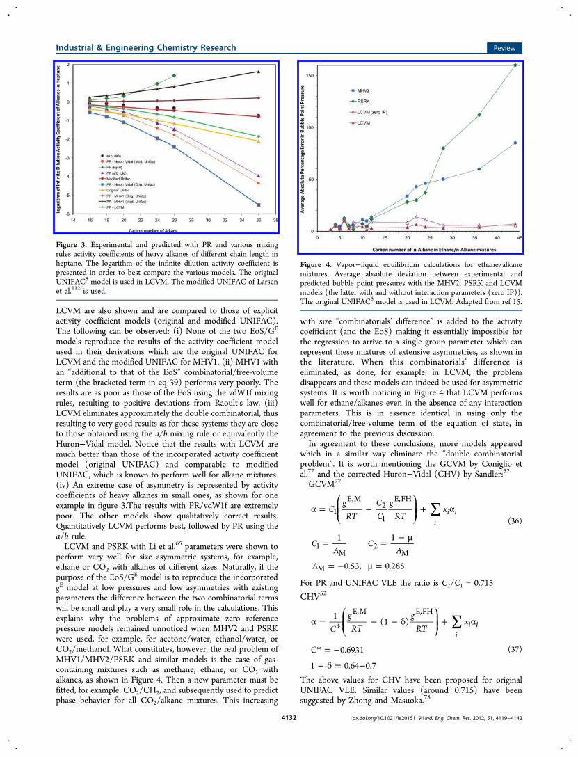
64, and 92, MHV1, PSRK, and MHV2 perform very poorly for(size) asymmetric mixtures like those containing gases (N2,CO2, ethane, or methane) with hydrocarbons of different size.Even though a new interaction parameter is estimated, forexample, for the group interaction CO2/−CH2− (in the case ofCO2/alkanes), these investigations clearly show that a singlegroup parameter cannot describe gas solubilities overextensive size asymmetries. The deviations are very high andincrease systematically with increasing size difference of themixture compounds (see also Figure 4). Boukouvalas et al.15

and Gmehling65 report that for ethane/dodecane thepercentage deviation in pressure is about 12−14% with eitherPSRK or MHV2 but it increases to over 30% for ethane/eicosane and beyond. Similarly, for CO2/alkanes, the deviationsin pressure are higher than 30% for CO2/eicosane and above.For methane/alkane mixtures, we have a similar picture. In thiscase, already for methane/nonane and beyond, the deviation inpressure is above 30% for MHV2 and in the case of PSRK formethane/hexadecane and beyond the deviation is also above30%. These are very disappointing results for the approximatezero reference pressure models.(4) It became soon apparent15,63,64,92 that even for low

pressure systems, such as mixtures of alkanes, the approximatezero reference pressure models do not fully reproduce the gE

model used in their derivation. The reproduction is satisfactoryfor mixtures of similar “size and energy” values, but as theasymmetry increases the reproduction of gE and especially ofthe activity coefficient is very poor. This topic was analyzed byKalospiros et al.67 who showed that the difference between thegE model (and the activity coefficient expression) obtained from

the EoS using the EoS/GE mixing rules and from the external gE

model (called here gE,M) is

Δ γ = γ − γ

= − α − αα

α−

αα

+ α − α − α − α

⎡⎣⎢

⎤⎦⎥

dqd

dqd

q q q q

(ln ) ln ln

( )( ) ( )

[ ( ) ( )] [ ( ) ( )]

i i i

ie

e ei i

M

(26)

∑

Δ = −

= α − α − α − α

⎛⎝⎜⎜

⎞⎠⎟⎟

gRT

gRT

gRT

q q x q q[ ( ) ( )] [ ( ) ( )]e

ii

ei i

E E E,M

(27)

From eqs 26 and 27 it is clear that the results especially forthe activity coefficients are very sensitive not only to the correctreproduction of the q function, but also its derivative withrespect to the reduced energy parameter. Especially thereproduction of this derivative is very poor from theapproximate zero reference pressure models. Kalospiros et al.67

concluded that in terms of the EoS/GE models, symmetricsystems should be considered those with similar reducedenergy values and only in this case can we expect goodreproduction of the underlying gE model. When the reducedenergy values from the two compounds are different andespecially as their difference increases, then we can expect poorreproduction of the gE,M by mixing rules like MHV1, MHV2,and PSRK. In reality, thus, we are talking about approximatezero reference pressure models, that is, the the actual referencepressure for these mixing rules (e.g., MHV1 and PSRK) is notexactly zero.67

The same conclusion can be reached in another way.Following Michelsen and Mollerup,44 who start from thefundamental equation,

∫− =gRT

gRT

VRT

PdE,P E,0

0

P E

(28)

it can be shown that at if we set P as infinite, then an almostexact expression can be obtained for the difference of gE atinfinite and zero pressure:

∑ ∑− = − αα

∞gRT

gRT

xbb

xln lni

ii i

ii

E, P E,0

(29)

This expression can be compared to the equivalent expressionwhich is obtained from the difference of infinite pressure andapproximate zero reference pressure models. In the case ofSRK, the difference between the Huron−Vidal and MHV1 orPSRK mixing rules is

∑

∑ ∑ ∑

− = − α − α

− α − α + ≈

∞gRT

gRT

x

q x xbb

xbb

ln 2( )

( ) ln ln

ii i

ii i

ii

i ii

i

E, P E,approx0

1

(30)

(since the terms −ln 2 and −q1 almost cancel each other esp.for PSRK).



Upon comparing eqs 30, that is, the approximate differencebetween infinite and zero pressure models, and 29, whichcorresponds to a more or less exact difference between the gE

values at infinite and zero pressure, we see that the term

∑ αα

x lni

ii

is missing in eq 30. This term is eliminated or diminished whenthe reduced energies of the compounds are similar, which is inaccordance to the terminology of “symmetric” systems ofKalospiros et al.67 The inspection of eqs 29 and 30 providesthus an additional proof of the approximate zero referencepressure character of models like MHV1, PSRK, and the like.Commenting on the four limitations discussed above,

possibly little can be done about the first one, while thepractical importance of the second limitation is somewhatunclear. On the other hand, limitations 3 and 4 are veryimportant and appear interconnected, although we will see thatthis is not always the case. This has led to a number of models,starting with LCVM, which aim to extend the applicability ofEoS/GE mixing rules to asymmetric systems. This topic has ledto many discussions in the literature both with respect to thesemodels’ capabilities and the explanation of their performance.We discuss in the coming section LCVM and some modelswhich followed, and we present a general explanation of theirperformance for asymmetric systems.2.5. LCVM and Related Models. The first model which

addressed specifically the limitation of size-asymmetric systemsis LCVM (linear combination of Vidal and Michelsen mixingrules) was proposed by Tassios and co-workers15 in 1994. Theauthors have presented the LCVM mixing rule for the energyparameter of the PR EoS as

∑ ∑α = λΑ

+ − λ + − λ + αΜ

⎛⎝⎜

⎞⎠⎟⎛⎝⎜⎜

⎞⎠⎟⎟

⎛⎝⎜

⎞⎠⎟A

gRT A

xbb

x1 1

lnV M

E M

il

i ii i

,

(31)

with AV = −0.623, AM = q1 = −0.52 and λ = 0.36 [originalUNIFAC], is a universal value obtained from ethane/alkaneVLE data. The translated PR and original UNIFAC are used,and the λ value depends on the specific choice of EoS and gE

model.LCVM was criticized in the literature41,47,48,51,52,54 due to its

apparent empirical nature:

• The model cannot be derived from the usual startingpoint of EoS/GE models, neither from eq 1a nor from eq1b.

• Being a combination of infinite and approximate zeroreference pressure models, it appears not to have aspecific reference pressure itself. Thus it is uncertainwhether a UNIFAC parameter table with parametersestimated based on low pressure data can be used.

• It contains an additional parameter, which thoughuniversal, seems to be connected to the specific cubicEoS and gE model used by the authors, thus it is notcertain that the mixing rule can be used with EoS and gE

models other than those employed in its development.• The whole approach appears rather empirical, for

example, why should this specific λ value be used? Notheoretical explanation was originally offered.

Despite these limitations, Tassios and co-workers haveshown in a series of publications15,63,66−74 that the LCVM

model can be used highly successfully for size asymmetricsystems such as methane, CO2, nitrogen, H2S, ethane withhydrocarbons of different sizes, as well as with polar com-pounds (alcohols, water, acids, etc), for predicting Henry’s lawconstants, solid−gas equilibria, gas condensates and infinitedilution activity coefficients of mixtures containing alkanes. Inaddition, the results for polar (symmetric and asymmetric) highpressure systems are at least as good as those of MHV2 and theWS mixing rules. Other researchers75 have also applied LCVMwith success, for example, in high pressure wax formation forpetroleum fluids. Soon it became apparent that the success ofLCVM could not be attributed to coincidence or cancellation oferrors. Some explanation should exist. Following the analysispresented by Kontogeorgis and co-workers,16,37,76 further veri-fied by Li et al.,65 we briefly outline below a phenomenologicalexplanation which can justify the success of both LCVM andseveral of the subsequent models.First, it can be shown that LCVM can be written in a form

equivalent to eq 31 as

∑

∑

α = − + α ⇒

α = − + + α

⎛⎝⎜⎜

⎞⎠⎟⎟

⎡⎣⎢⎢⎛⎝⎜⎜

⎞⎠⎟⎟

⎤⎦⎥⎥

CgRT

CC

gRT

x

Cg

RTCC

gRT

gRT

x

ii i

ii i

1

E,M2

1

E,FH

1

E,comb,M2

1

E,FH E,res,M

(32)

where

= λ + − λ

= − λ

CA A

CA

1

1

1V M

2M

= − = −A A0.623, 0.52V M

The FH combinatorial is given in eq 20d and for λ = 0.36 ⇒C2/C1 = 0.68 “comb” and “res” are the combinatorial andresidual terms of the external activity coefficient model used, forexample, UNIFAC.The MHV1 model, eq 20, can also be written in a similar way

when an external gE model like UNIQUAC and UNIFAC isused which has separate combinatorial and residual terms:

∑

∑

α = − + α ⇒

α = − + + α

⎛⎝⎜⎜

⎞⎠⎟⎟

⎡⎣⎢⎢⎛⎝⎜⎜

⎞⎠⎟⎟

⎤⎦⎥⎥

qgRT

gRT

x

qg

RTg

RTg

RTx

1

1

ii i

ii i

1

E,M E,FH

1

E,comb,M E,FH E,res,M

(33)

In most cases we can ignore the Staverman−Guggenheimcontribution to the combinatorial term as it typicallycontributes little to the activity coefficient value, when physicalvalues are used for the van der Waals volume and area. Then,the combinatorial contributions to the excess Gibbs energyfrom UNIQUAC/UNIFAC and the various versions ofmodified UNIFAC are expressed as the following:



Original UNIFAC/UNIQUAC

∑ ∑= =∑

gRT

xrr

xrx r

ln lni

ii

ii

i

i i i

E,comb,M

(34a)

Modified UNIFAC (x = 2/3 for Lyngby version and x = 3/4 forDortmund version)

∑ ∑= =∑

gRT

xrr

xrx r

ln lni

iix

xi

iix

i i ix

E,comb,M

(34b)

Thus, it can be seen that the combinatorial terms from theexternal activity coefficient model, for example, eqs 34a and34b, and from the FH-type one stemming from the EoS at theapproximate zero reference pressure (eq 20c) are similar infunctionality. But are they similar in magnitude as well? Ideally,and for the purpose of obtaining a purely energetic parameterespecially when new interaction parameters are estimated, this“difference of combinatorial terms” from the EoS and from theexternal activity coefficient model should be zero. “The twocombinatorials should cancel”, as stated by Mollerup10 morethan 20 years ago. In this way, eq 1a, in the case of approximatezero reference pressure models, could be written as

∑

=

= =

⎛⎝⎜⎜

⎞⎠⎟⎟

⎛⎝⎜⎜

⎞⎠⎟⎟

⎛⎝⎜⎜

⎞⎠⎟⎟

⎛⎝⎜

⎞⎠⎟

gRT

gRT

gRT

xbb

lni

ii

E,comb,M E,comb,EoS

approx.zeroE,FH

(35a)

=⎛⎝⎜⎜

⎞⎠⎟⎟

⎛⎝⎜⎜

⎞⎠⎟⎟

gRT

gRT

E,res,M E,res,EoS

approx.zero (35b)

Notice that in the case of Huron−Vidal and Wong−Sandlermixing rules, eqs 1a and 1b reduce essentially to eq 35b, asexplained previously.Unfortunately, as shown by Kontogeorgis and Vlamos76 and by

Li et al.65 this “difference of combinatorials” does not cancel out. Itis small for systems with similar asymmetry but as the size and

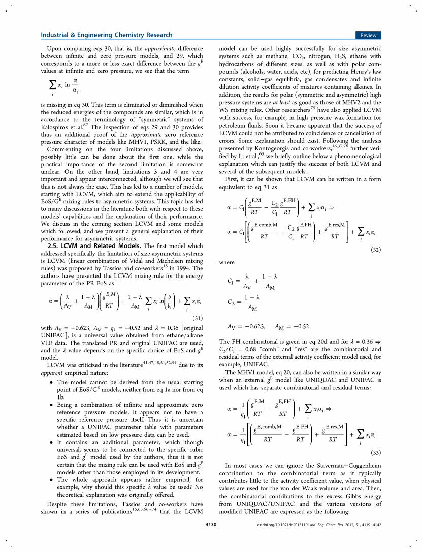
energy differences between the mixture components increase, thenthis difference of the combinatorial terms (i.e., the combinatorialcontribution to the activity coefficient from EoS minus that fromthe external gE model) increases as well, as shown in the above-mentioned publications.76,65 In the same references76,65 thefollowing are also shown: (i) The LCVM with the correctionfactor C2/C1 = 0.68 minimizes the combinatorial differencebetween the FH term from the EoS and the original UNIFACcombinatorial. A correction factor C2/C1 = 0.3 (corresponding to λequal to 0.7) minimizes again the combinatorials’ difference whenthe combinatorial term of the modified UNIFAC is used.Interestingly, this λ-value for a modified UNIFAC has beenalready recommended by Boukouvalas et al.15 in the originalpublication of LCVM (without explanation). (ii) PSRK with fittedvan der Waals volume (r) parameters can also minimize thecombinatorial difference between the combinatorial term in eq 34band the FH term.Additional evidence is provided by the results shown in

Table 6 as well as Figures 2 and 3 for mixtures of alkanes with

different chain length. These are the same systems as shown inTable 4 and in Figure 1 but now the results of MHV1 and

Table 6. Percentage Absolute Deviation between Experimental and Calculated Activity Coefficients at Infinite Dilution forn-Butane and n-Heptane in Various Alkanes Using the PR EoS and the MHV1 and LCVM Mixing Rules. For Comparison theDeviations with Original and Modified UNIFAC Combinatorials5,112 Are Also Given

alkane Or.UNIFAC Mod.UNIFAC PR-MHV1 with Or.UNIFAC PR-MHV1 with modified UNIFAC PR-LCVM (PR-a/b rule)

n-Butane20 39 16 39 98 0.9 (0.6)22 41 17 50 120 0.6 (1.1)24 40 13 64 150 5.8 (2.0)28 43 13 77 187 5.3 (2.5)32 45 11 95 234 7.0 (5.3)36 46 10 113 285 8.4 (9.3)average 42 13 73 179 4.7 (3.5)

n-Heptane20 21 6.8 15 50 4.0 (5.3)22 25 9.1 17 46 7.0 (11.1)24 24 5.2 26 63 3.4 (9.3)28 26 3.0 38 88 2.0 (11.7)32 28 1.9 50 114 1.7 (15.6)36 30 0.2 62 144 0.3 (19.3)Average 26 4.4 35 83 3.1 (12.0)

Figure 2. Experimental and predicted with PR and various mixingrules activity coefficients of hexane in alkanes of different chain length.The original UNIFAC5 model is used in LCVM.




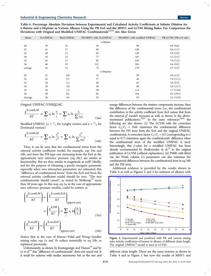
LCVM are also shown and are compared to those of explicitactivity coefficient models (original and modified UNIFAC).The following can be observed: (i) None of the two EoS/GE

models reproduce the results of the activity coefficient modelused in their derivations which are the original UNIFAC forLCVM and the modified UNIFAC for MHV1. (ii) MHV1 withan “additional to that of the EoS” combinatorial/free-volumeterm (the bracketed term in eq 39) performs very poorly. Theresults are as poor as those of the EoS using the vdW1f mixingrules, resulting to positive deviations from Raoult’s law. (iii)LCVM eliminates approximately the double combinatorial, thusresulting to very good results as for these systems they are closeto those obtained using the a/b mixing rule or equivalently theHuron−Vidal model. Notice that the results with LCVM aremuch better than those of the incorporated activity coefficientmodel (original UNIFAC) and comparable to modifiedUNIFAC, which is known to perform well for alkane mixtures.(iv) An extreme case of asymmetry is represented by activitycoefficients of heavy alkanes in small ones, as shown for oneexample in figure 3.The results with PR/vdW1f are extremelypoor. The other models show qualitatively correct results.Quantitatively LCVM performs best, followed by PR using thea/b rule.LCVM and PSRK with Li et al.65 parameters were shown to

perform very well for size asymmetric systems, for example,ethane or CO2 with alkanes of different sizes. Naturally, if thepurpose of the EoS/GE model is to reproduce the incorporatedgE model at low pressures and low asymmetries with existingparameters the difference between the two combinatorial termswill be small and play a very small role in the calculations. Thisexplains why the problems of approximate zero referencepressure models remained unnoticed when MHV2 and PSRKwere used, for example, for acetone/water, ethanol/water, orCO2/methanol. What constitutes, however, the real problem ofMHV1/MHV2/PSRK and similar models is the case of gas-containing mixtures such as methane, ethane, or CO2 withalkanes, as shown in Figure 4. Then a new parameter must befitted, for example, CO2/CH2, and subsequently used to predictphase behavior for all CO2/alkane mixtures. This increasing

with size “combinatorials’ difference” is added to the activitycoefficient (and the EoS) making it essentially impossible forthe regression to arrive to a single group parameter which canrepresent these mixtures of extensive asymmetries, as shown inthe literature. When this combinatorials’ difference iseliminated, as done, for example, in LCVM, the problemdisappears and these models can indeed be used for asymmetricsystems. It is worth noticing in Figure 4 that LCVM performswell for ethane/alkanes even in the absence of any interactionparameters. This is in essence identical in using only thecombinatorial/free-volume term of the equation of state, inagreement to the previous discussion.In agreement to these conclusions, more models appeared

which in a similar way eliminate the “double combinatorialproblem”. It is worth mentioning the GCVM by Coniglio etal.77 and the corrected Huron−Vidal (CHV) by Sandler:52

GCVM77

∑α = − + α⎛⎝⎜⎜

⎞⎠⎟⎟C

gRT

CC

gRT

xi

i i1

E,M2

1

E,FH

(36)

= = − μ

= − μ =

CA

CA

A

1 1

0.53, 0.285

1M

2M

M

For PR and UNIFAC VLE the ratio is C2/C1 = 0.715

CHV52

∑α = * − − δ + α⎛⎝⎜⎜

⎞⎠⎟⎟C

gRT

gRT

x1

(1 )i

i iE,M E,FH

* = −C 0.6931 (37)

− δ = −1 0.64 0.7The above values for CHV have been proposed for originalUNIFAC VLE. Similar values (around 0.715) have beensuggested by Zhong and Masuoka.78

Figure 3. Experimental and predicted with PR and various mixingrules activity coefficients of heavy alkanes of different chain length inheptane. The logarithm of the infinite dilution activity coefficient ispresented in order to best compare the various models. The originalUNIFAC5 model is used in LCVM. The modified UNIFAC of Larsenet al.112 is used.

Figure 4. Vapor−liquid equilibrium calculations for ethane/alkanemixtures. Average absolute deviation between experimental andpredicted bubble point pressures with the MHV2, PSRK and LCVMmodels (the latter with and without interaction parameters (zero IP)).The original UNIFAC5 model is used in LCVM. Adapted from ref 15.





The similarity of eqs 36 and 37 to LCVM, eq 32, isstriking! Even the correction coefficients are similar,illustrating further in agreement with the double combina-torial difference concept, that this correction coefficient ismore related to which gE model is used (e.g., original ormodified UNIFAC) rather than which cubic EoS (sinceboth SRK and PR at approximate zero reference pressureinclude the FH-type term).An additional evidence of the above explanation on the role

of the “double combinatorial” can be offered by looking at theactivity coefficient equation from LCVM and the relatedmodels, for example, GCVM and CHV.For CHV (and similarly also for the other models) using

SRK, the infinite dilution activity coefficient of a compound in abinary system is

γ = γ + γ =−−

+

−−−

++

+

+−

++ −

*+

γ − − δ γ + −*

+γ

∞ −

⎜ ⎟

⎜ ⎟

⎛⎝⎜

⎞⎠⎟

⎛⎝⎜

⎞⎠⎟

⎛⎝⎜

⎞⎠⎟

⎛⎝⎜

⎞⎠⎟

⎛⎝⎜⎜

⎞⎠⎟⎟

⎛⎝

⎞⎠

⎛⎝⎜

⎞⎠⎟

⎛⎝

⎞⎠

⎛⎝⎜

⎞⎠⎟

V bV b

V bV b

ab RT

ab RT

V b V b

V b V CV b

V

CV b

V

ln ln ln ln 1

ln1

1

1ln

[ln (1 ) ln ]1

ln ln

bV

bV

1 1comb FV

1res 1 1

2 2

1 1

2 2

1

1

2

2

1 2 2 1

22

2 2

2 2

2

1comb,M

1FH

2 2

21res,M

1

1

2

2

(38)

As compared to the expression under the same conditions forMHV1:

γ = γ + γ =−−

+

−−−

++

++

−+

+ − +γ

− γ + − +γ

∞ − ⎛⎝⎜

⎞⎠⎟

⎛⎝⎜

⎞⎠⎟

⎛⎝⎜

⎞⎠⎟

⎛⎝⎜

⎞⎠⎟

⎛⎝⎜⎜

⎞⎠⎟⎟

⎛⎝⎜

⎞⎠⎟

⎛⎝⎜

⎞⎠⎟

⎛⎝⎜

⎞⎠⎟

⎛⎝⎜

⎞⎠⎟

V bV b

V bV b

ab RT

ab RT

V b V b

V b V AV b

V

AV b

V

ln ln ln ln 1

ln1

1

1ln [ln

ln ]1

ln ln

bV

bV

FH

1 1comb FV

1res 1 1

2 2

1 1

2 2

1

1

2

2

1 2 2 1

22

2 2 M

2 2

21comb,M

1M

2 2

21res,M

1

1

2

2

(39)

Upon comparing eqs 38 and 39 with eqs 5a−5c, we notethat the residual term is the same as for the SRK/Huron−Vidal. Moreover, the combinatorial/free-volume terms ofcubic EoS using the various mixing rules differ only by thebracketed terms in eqs 38 and 39 included in MHV1 andCHV. This is what we have indicated as the combinatorialterms’ difference. Indeed, as can be expected based on whatwe discussed previously, if this combinatorials’ difference issmall, then the combinatorial/free-volume part of the cubicEoS performs quite well for athermal mixtures like foractivity coefficients with alkane systems. As shown before,the combinatorial/free-volume of cubic EoS (SRK and PR)describes satisfactorily (at least qualitatively, often alsoquantitatively) the size/shape effects of alkane mixtures (in

this case, recall that the residual term is zero). For CHV,LCVM, and GCVM the bracketed terms (difference ofcombinatorials) are close to zero, while the correspondingbracketed term of MHV1 is not zero. Moreover, thecombinatorials’ difference in MHV1 increases with sizeasymmetry, thus explaining why MHV1 and related modelsresult in unphysical high (even above unity) activitycoefficients for alkane mixtures (see also the results in Table 6and Figures 2 and 3).It appears that LCVM, GCVM, CHV and related models

obey in reality eq 35a, that is, they reproduce the gE,comb of theincorporated model, or in reality they “correct” thecombinatorial activity coefficient of the incorporated gE

model. In this way the residual (energetic) term of EoS isallowed to “do the remaining job”, that is, to describe phasebehavior for complex mixtures using interaction parameters,either via existing (e.g., UNIFAC) or new interactionparameters (for gas-containing mixtures).The approach of eliminating the “double combinatorial” has

resulted in a new trend in the development of EoS/GE modelsmaking them suitable also for asymmetric systems. Two morerecent approaches have been developed which essentially relyon the same principle as outlined above.The first approach by Gmehling and co-workers79−87 is to

develop a new type of PSRK as well as an EoS/GE based ona translated PR (called VTPR) both of which eliminatethe double combinatorial in eq 33 from the start. Thus, theresulting mixing rule resembles the one obtained at infinitepressure with two differences: the q1 value corresponds to thezero reference pressure models and a nonlinear mixing rule isused for the covolume:

∑α = + α

= −

⎛⎝⎜⎜

⎞⎠⎟⎟q

gRT

x

q

1

0.64663i

i i1

E,res,M

1 (40a)

(the above q1 is for PSRK, for VTPR q1 = −0.53087) with

∑ ∑=

=+⎛

⎝⎜⎜

⎞

⎠⎟⎟

b x x b

bb b

2

i ji j ij

iji j3/4 3/4 4/3

(40b)

Similarly, Voutsas et al.88−91 proposed the UMR-PR model, anEoS/GE mixing rule similar to VTPR but keeping theStaverman−Guggenheim (SG) part of the combinatorial termand they have used a slightly different expression for thecovolume:

∑α = + + α

= −

⎛⎝⎜⎜

⎞⎠⎟⎟q

gRT

gRT

x

q

1

0.53i

i i1

E,SG,M E,res,M

1 (41a)



with

∑ ∑=

=+⎛

⎝⎜⎜

⎞

⎠⎟⎟

b x x b

bb b

2

i ji j ij

iji j1/2 1/2 2

(41b)

It may appear somewhat surprising that the authors have noteliminated the full difference of the combinatorials but chose tokeep part of the combinatorial contribution, the one that usuallyhas the least effect. Otherwise the approach is similar to the one ofGmehling and co-workers for VTPR. Nevertheless, unlike VTPR,in the UMR-PR the existing UNIFAC parameters can be used.New parameters are fitted for the group interactions in VTPR.A similar model to UMR-PR but coupled with SRK has been

recently proposed by Chen et al.92 using a 2/3 exponent in theb’s in eq 41b. Equally satisfactory results as for UMR-PR areobtained for gas/alkanes.The second approach is to introduce an lij parameter in the

covolume combining rule and maintain the same form for themixing rule for the energy parameter as for the approximatezero reference pressure models. For example, Gani and co-workers64,92 used the MHV1 model with

=+

−bb b

l2

(1 )iji j

ij (42)

A constant lij = 0.3 could describe well a series of asymmetricsystems of CO2 and fatty acid esters.The use of a combining rule differing from the linear one for the

covolume and the role of lij (correction to the covolume mixingrule) may be significant, as discussed by Kontogeorgis et al.38 Theyshowed that using an lij = 0.02 (and kij = 0) PR can correlateethane/alkanes using the vdW1f mixing rules very well.The inspection of the general equation for the activity coefficient

expression from cubic EoS provides some insight on thesignificance of the mixing rule for the covolume parameter. For PR,

γ =−−

+ −− −

+α + +

+ −

−α + +

+ −

+α − + + −

⎡⎣⎢

⎤⎦⎥

⎡⎣⎢

⎤⎦⎥

⎡⎣⎢

⎤⎦⎥

⎡⎣⎢

⎤⎦⎥

V bV b

V bV b

V bV b

V bV b

bV VbV V b b V b

ln ln 1

2 2ln

(1 2 )(1 2 )

2 2ln

(1 2 )(1 2 )

( )( ) ( )

ii i i i

i i i

i i

i

i i(43)

where

∑

∑

α =

= − +

= − +

α = + −⎡

⎣⎢⎤⎦⎥

abRT

b b x b

a a x a

abRT

aa

bb

2

2

1

ij

j ij

ij

j ij

ii i

Equation 43 is simplified if a linear mixing rule is used for thecovolume:

∑=b x bi

i i

Then,

γ =−−

+ −−−

+α + +

+ −−

α

+ ++ −

+α −+ + −

⎡⎣⎢

⎤⎦⎥

⎡⎣⎢

⎤⎦⎥

⎡⎣⎢

⎤⎦⎥

⎡⎣⎢

⎤⎦⎥

V bV b

V bV b

V bV b

V bV b

bV VbV V b b V b

ln ln 1

2 2ln

(1 2 )(1 2 ) 2 2

ln(1 2 )(1 2 )

( )( ) ( )

ii i i i

i i i

i i

i

i i

(44a)

∑

α =

= − +

α = + −⎡⎣⎢

⎤⎦⎥

abRT

a a x a

abRT

aa

bb

2

1

ij

j ij

ii i

At infinite dilution, eq 44a can be written as

γ =−−

+ −− −

−

++ ++ −

++ −

+ −

− + −

+ ++ −

∞ ⎡⎣⎢

⎤⎦⎥

⎡⎣⎢

⎤⎦⎥

⎡⎣⎢

⎤⎦⎥

⎛⎝⎜⎜

⎞⎠⎟⎟

⎛⎝⎜

⎞⎠⎟

⎡⎣⎢

⎤⎦⎥

V bV b

V b bV b

ab RT

V bV b

ab RT

V b V b V b

V V b b

ab RT

aa

bb

V bV b

ln ln 1( 2 )

2 2ln

(1 2 )(1 2 )

2

2

212

ln(1 2 )(1 2 )

11 1

2 2

1 2 12

2 2

1

1

1 1

1 2

2

2

1 2 2 2 2 12

22

2 2 22

2

2

12

2

12

2

2 2

2 2 (44b)

Upon comparing eqs 43 and 44, it can be seen that themixing rule for the covolume parameter appears in all terms ofthe EoS expression for the activity coefficient. This may justifywhy the use of an lij or a combining rule other than thearithmetic mean for the covolume parameter can effectively“correct” both the combinatorial and the residual contributionsof the equation of state.

3. DISCUSSIONA general discussion on the capabilities and limitations of EoS/GE mixing rules is offered in this section, supported by someadditional references. Table 7 shows a comparative presentationof the characteristics of some of the most well-known mixingrules.The most important conclusions from the investigations on

EoS/GE mixing rules can be summarized as follows:(1) Huron−Vidal mixing rules combined with a cubic EoS

(SRK or PR) constitute an excellent fitting tool, both forcorrelating phase behavior (including LLE and VLLE) ofmixtures of complex compounds and for predicting multiphasebehavior for multicomponent mixtures. In particular the NRTL



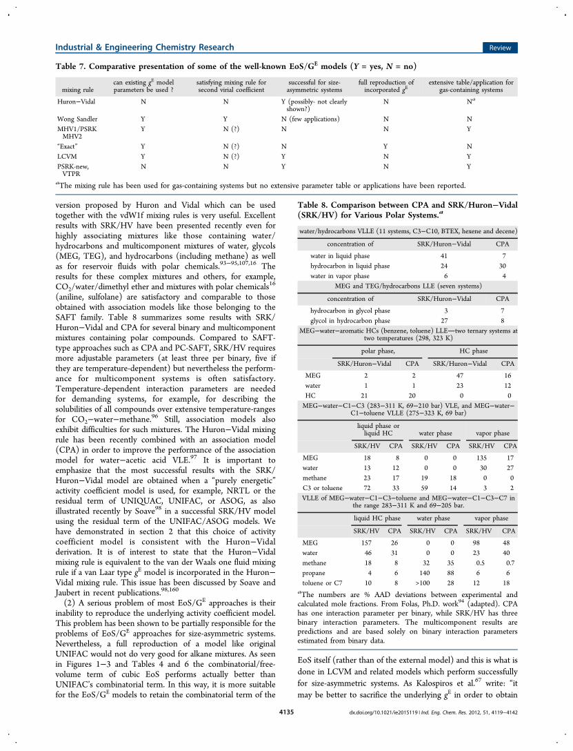
version proposed by Huron and Vidal which can be usedtogether with the vdW1f mixing rules is very useful. Excellentresults with SRK/HV have been presented recently even forhighly associating mixtures like those containing water/hydrocarbons and multicomponent mixtures of water, glycols(MEG, TEG), and hydrocarbons (including methane) as wellas for reservoir fluids with polar chemicals.93−95,107,16 Theresults for these complex mixtures and others, for example,CO2/water/dimethyl ether and mixtures with polar chemicals16

(aniline, sulfolane) are satisfactory and comparable to thoseobtained with association models like those belonging to theSAFT family. Table 8 summarizes some results with SRK/Huron−Vidal and CPA for several binary and multicomponentmixtures containing polar compounds. Compared to SAFT-type approaches such as CPA and PC-SAFT, SRK/HV requiresmore adjustable parameters (at least three per binary, five ifthey are temperature-dependent) but nevertheless the perform-ance for multicomponent systems is often satisfactory.Temperature-dependent interaction parameters are neededfor demanding systems, for example, for describing thesolubilities of all compounds over extensive temperature-rangesfor CO2−water−methane.96 Still, association models alsoexhibit difficulties for such mixtures. The Huron−Vidal mixingrule has been recently combined with an association model(CPA) in order to improve the performance of the associationmodel for water−acetic acid VLE.97 It is important toemphasize that the most successful results with the SRK/Huron−Vidal model are obtained when a “purely energetic”activity coefficient model is used, for example, NRTL or theresidual term of UNIQUAC, UNIFAC, or ASOG, as alsoillustrated recently by Soave98 in a successful SRK/HV modelusing the residual term of the UNIFAC/ASOG models. Wehave demonstrated in section 2 that this choice of activitycoefficient model is consistent with the Huron−Vidalderivation. It is of interest to state that the Huron−Vidalmixing rule is equivalent to the van der Waals one fluid mixingrule if a van Laar type gE model is incorporated in the Huron−Vidal mixing rule. This issue has been discussed by Soave andJaubert in recent publications.98,160

(2) A serious problem of most EoS/GE approaches is theirinability to reproduce the underlying activity coefficient model.This problem has been shown to be partially responsible for theproblems of EoS/GE approaches for size-asymmetric systems.Nevertheless, a full reproduction of a model like originalUNIFAC would not do very good for alkane mixtures. As seenin Figures 1−3 and Tables 4 and 6 the combinatorial/free-volume term of cubic EoS performs actually better thanUNIFAC’s combinatorial term. In this way, it is more suitablefor the EoS/GE models to retain the combinatorial term of the

EoS itself (rather than of the external model) and this is what isdone in LCVM and related models which perform successfullyfor size-asymmetric systems. As Kalospiros et al.67 write: “itmay be better to sacrifice the underlying gE in order to obtain

Table 7. Comparative presentation of some of the well-known EoS/GE models (Y = yes, N = no)

mixing rulecan existing gE modelparameters be used ?

satisfying mixing rule forsecond virial coefficient

successful for size-asymmetric systems

full reproduction ofincorporated gE

extensive table/application forgas-containing systems

Huron−Vidal N N Y (possibly- not clearlyshown?)

N Na

Wong Sandler Y Y N (few applications) N NMHV1/PSRKMHV2

Y N (?) N N Y

“Exact” Y N (?) N Y NLCVM Y N (?) Y N YPSRK-new,VTPR

N N Y N Y

aThe mixing rule has been used for gas-containing systems but no extensive parameter table or applications have been reported.

Table 8. Comparison between CPA and SRK/Huron−Vidal(SRK/HV) for Various Polar Systems.a

water/hydrocarbons VLLE (11 systems, C3−C10, BTEX, hexene and decene)

concentration of SRK/Huron−Vidal CPA

water in liquid phase 41 7hydrocarbon in liquid phase 24 30water in vapor phase 6 4

MEG and TEG/hydrocarbons LLE (seven systems)

concentration of SRK/Huron−Vidal CPA

hydrocarbon in glycol phase 3 7glycol in hydrocarbon phase 27 8

MEG−water−aromatic HCs (benzene, toluene) LLEtwo ternary systems attwo temperatures (298, 323 K)

polar phase, HC phase

SRK/Huron−Vidal CPA SRK/Huron−Vidal CPA

MEG 2 2 47 16water 1 1 23 12HC 21 20 0 0MEG−water−C1−C3 (283−311 K, 69−210 bar) VLE, and MEG−water−

C1−toluene VLLE (275−323 K, 69 bar)

liquid phase orliquid HC water phase vapor phase

SRK/HV CPA SRK/HV CPA SRK/HV CPA

MEG 18 8 0 0 135 17water 13 12 0 0 30 27methane 23 17 19 18 0 0C3 or toluene 72 33 59 14 3 2VLLE of MEG−water−C1−C3−toluene and MEG−water−C1−C3−C7 in

the range 283−311 K and 69−205 bar.

liquid HC phase water phase vapor phase

SRK/HV CPA SRK/HV CPA SRK/HV CPA

MEG 157 26 0 0 98 48water 46 31 0 0 23 40methane 18 8 32 35 0.5 0.7propane 4 6 140 88 6 6toluene or C7 10 8 >100 28 12 18

aThe numbers are % AAD deviations between experimental andcalculated mole fractions. From Folas, Ph.D. work94 (adapted). CPAhas one interaction parameter per binary, while SRK/HV has threebinary interaction parameters. The multicomponent results arepredictions and are based solely on binary interaction parametersestimated from binary data.



overall good results”. While we recognize that some maydisagree with this, the capabilities of the combinatorial/free-volume term of the EoS support this statement.(3) We have provided in section 2 several references and

arguments which underline the importance of eliminating thedouble combinatorial term in the approximate zero referencepressure models so that the resulting EoS/GE approaches canbe used successfully for size-asymmetric systems. Indeedmodels like CHV and LCVM perform best for such systems.The literature is rich with such approaches, for example, Zhongand Masuoka78 have proposed the following mixing rule:

∑α = + − + α⎛⎝⎜⎜

⎞⎠⎟⎟q

fgRT

gRT

x1

(1 )i

i i1

E,M E,FH

(45)

Although in eq 45 the correction factor is included in theexternal model term rather than in the FH term, thesignificance is the same and the average value reported ( f =0.36) is equivalent to the corrections factors used in the othermodels. Zhong and Masuoka78 present also correlations of thef-parameter with the carbon number for some gas/alkanefamilies.Neau and co-workers102,103 have recently proposed an

EoS/GE mixing rule which, though not clearly stated as such,again uses the principle of the elimination of the doublecombinatorial. They employ PR with a generalized (group-based) NRTL that includes a combinatorial term based onsegment fractions (van der Waals volumes). This is identicalwith the combinatorial term that is included in the mixing rulethey propose:

∑ ∑α = − + α⎛

⎝⎜⎜

⎞

⎠⎟⎟C

gRT

xrr

x1

lni

ii

ii i

E,M

(46)

Thus, the two combinatorial terms are eliminated and theresulting model has the same combinatorial/free-volume termas the EoS itself. The resulting PR-NRTL is in essence aHuron−Vidal type mixing rule. Thus, while we agree with theauthors’ statement that the final model accounts for theentropic effects correctly this does not happen because of thenew version of NRTL that the authors use. It is rather due tothe elimination of the double combinatorial in eq 46. Neau etal.99,100 show that their new model gives good results, which weexpect that they will be similar to those of other EoS/GE

models with the same qualitative characteristics. It is interestingto note that their model can represent the minimum of thehydrocarbon solubility in water with temperature which, as ithas been shown,19 it can be also described by the Huron−Vidalmixing rule in general. A similar model presented earlier by thesame authors101−104 is again based on a variation of eq 46 usingthe generalized NRTL. In those earlier works MHV1 is usedwith covolumes which are estimated via the van der Waalsvolumes (instead of the critical properties). The result is againessentially an elimination of the double combinatorial. Anadditional indication for the “double combinatorial” problemfor size-asymmetric systems can be extracted from the work ofLermite and Vidal25,26 who used an MHV1 (constant-packingbased) approach but (possibly inspired by the Huron−Vidal

mixing rule) kept only the residual term of UNIQUAC orUNIFAC, thus their mixing rule is

∑α = − + α⎛⎝⎜⎜

⎞⎠⎟⎟q

gRT

gRT

x1

ii i

1

E,M,res E,FH

(47)

New interaction parameters are fitted but, as might be expected,the results are not satisfactory for asymmetric gas-containingmixtures. This conclusion is again in agreement with the“double combinatorial” explanation. In this case we have asingle “extra (to that of the EoS)” combinatorial term. It is theFH-term (originated from the constant packing fractionassumption) which is added to the combinatorial/free-volumeterm of EoS and results to an overcorrection of thecombinatorial/free-volume term from the EoS. On the otherhand, the same authors27,39 used correctly in combination withthe Huron−Vidal mixing rule:

∑α = + α⎛⎝⎜⎜

⎞⎠⎟⎟q

gRT

x1

ii i

1

E,M,res

(48)

the residual term of UNIQUAC or UNIFAC. Equation 48 isthe Huron−Vidal mixing rule and essentially also the mixingrule used in PSRK-new and VTPR. The results are satisfactoryfor a variety of mixtures including size-asymmetric ones (newparameters must be fitted but they can be group-based ones).Finally, we should mention that PSRK-new, VTPR, and

UMR-PR are quite similar models. All three models essentiallyeliminate the double combinatorial and use a different than theusual arithmetic mean mixing rule rule for the covolumeparameter. As shown by Chen et al.,79 the importance of thiscombining rule (eq 40b) over the arithmetic mean one is rathersmall and it is the elimination of the double combinatorialwhich is the main reason for the successful results for size-asymmetric systems. Voutsas (2010, private communication)verified that by indicating that the new combining rule for thecovolume (eq 41b) is particularly important for polymericsystems, otherwise a linear mixing rule could as well be used.New parameters are regressed in VTPR while UMR-PRemploys the existing UNIFAC interaction parameters.There are many studies in the literature that indicate that

combining rules other than the linear one for the covolume canresult in improved results for polymer mixtures. For example,Zhong and Masuoka105 used the simple form of SRK/Huron−Vidal shown in eq 48 without any residual term. This meansthat they used essentially the a/b mixing rule together with theWong−Sandler mixing rule for the second virial coefficient, thatis, eqs 11 and 14a. They showed (and it was verified by Louliand Tassios106) that excellent correlation results are obtainedfor polymer−solvent VLE using a single kij per system. Theperformance is better than with other mixing rules. The successwas considered surprising in the articles by Zhong−Masuoka105

and Louli−Tassios106 but we believe it can be explained by thefact that the a/b mixing rule isolates and illustrates that thecombinatorial/free volume contribution from cubic EoS isrepresented adequately, as shown by the results for mixtureswith alkanes differing significantly in size (see Figures 1−3 andTables 4 and 6).(4) Liquid−liquid equilibrium studies using the EoS/GE

models have been presented by several authors110,111,117−124

and particularly interesting are the investigations by Escobedo−Alvarado and Sandler110 and Knudsen et al.111 It is shown inthese works that EoS/GE mixing rules such as MHV2 and



Wong−Sandler, especially when combined with molecular-based local composition models (NRTL, UNIQUAC) cancorrelate well LLE of complex mixtures. The results aresatisfactory for high pressure LLE based on low pressureobtained parameters. In this sense and also because of theirbetter temperature dependency (which permits more successfulextrapolations) EoS/GE models are superior to the underlyinggE model.110,122 For strongly hydrogen bonding systems,however, such as 2-butanol/water and 2-butoxyethanol/watera significant number of adjustable parameters is needed fordescribing the observed closed loop behavior and its depend-ency on temperature and pressure. Predictions for multi-component systems based solely on binary data are notsatisfactory.111

(5) Compared to the large number of studies on phasebehavior, relatively few investigations have been published forthermal properties (heat of mixing, heat capacities). Djordjevicet al.136 in their review article discuss particularly theperformance of several EoS/GE mixing rules for enthalpiesand heat capacities. Their most important conclusion is, that forall mixing rules, the need of temperature dependent adjustableparameters is crucial for describing accurately thermal proper-ties. In general, as Ghosh135 discusses, the excess enthalpiesproduced from the EoS/GE mixing rules are more positivethan those obtained from the incorporated activity coefficientmodels.More specifically, both the PSRK and VTPR models have

been tested to both enthalpies and heat capacities andqualitatively good results have been reported by Gmehlingand co-workers,79,81,82,84,86,87 especially for VTPR. This can bepartially attributed to the good temperature dependency of theinteraction parameters and the inclusion of thermal data in theUNIFAC parameter estimation. Deviations between 4 and 8%have been reported for the new PSRK of Chen et al.79 forthe excess enthalpies of alkanes with alkanes, ketones andmethanol. Moreover, VTPR is shown to perform clearly betterthan PSRK for excess enthalpies for a wide range of families(alkanes+aromatics, alkanes+ketones, aromatics+ketones, esters+alkanes, esters+aromatics).Good excess enthalpies have been presented with UMR-PR89

for a few systems using temperature dependent interactionparameters. Detailed studies on excess enthalpies with theWong−Sandler and MHV1 mixing rules have been presentedby Sandler and co-workers,125,126 Zhong and Masuoka,127 andOhta.128 Zhong and Masuoka127 showed that MHV1 cannotreproduce the excess enthalpies of the incorporated activitycoefficient model but a modification similar to eq 45 performedmuch better both for asymmetric systems VLE and for excessenthalpies. Good excess enthalpies have been reported with thismodified MHV1 model for a wide range of alcohol−hydrocarbon, alcohol−water, and alcohol−ketone systems.The results are comparable to those of modified UNIFAC.Ohta128 compared MHV1 and Wong−Sandler rules and foundacceptable and similar excess enthalpies (& VLE) for a numberof systems, including a few ternary excess enthalpies, usingtemperature dependent parameters.Sandler and co-workers125,126 have also studied the MHV1

and Wong−Sandler mixing rules for excess enthalpies. Theyfound125 that, for four highly nonideal systems, the models cancalculate VLE and excess enthalpies separately but not both.The best way to regress parameters for these models is by usingsimultaneously VLE and excess enthalpy data (and not any ofthis type of data alone). Especially excess enthalpy data are

useful for selecting the best set of adjustable parameters.126

Moreover, they showed that simultaneous correlation of VLEand excess enthalpies at one temperature is possible butextrapolation at other temperatures did not result in accurateprediction of either VLE or excess enthalpies. Better results areobtained for less nonideal systems.126 Because of the pressuredependency, the Wong−Sandler (and other mixing rules)should be preferred over the incorporated activity coefficientmodel for capturing the pressure dependency of thermalproperties.(6) Another application of EoS/GE models is in the

prediction of solid−gas equilibria. This is an important typeof phase behavior, crucial in the design of supercritical fluidextraction. These systems are challenging due to theasymmetric nature of the gas and the solute, both in terms ofmolecular size and intermolecular forces but also because oftenthe pure component properties (critical properties and vaporpressures) of solids are not available and their estimations e.g.from group contribution methods are not always reliable. Anadditional issue is the frequent need of cosolvents for increasingthe solubility of the solute in the supercritical fluid, thus themodeling of supercritical fluid/cocolvent/solute is of impor-tance. The MHV1, Huron−Vidal, Wong−Sandler, LCVM, andUMR-PR mixing rules have been used for solid−gasequilibrium calculations.73,74,89,129−132

The applications are not very extensive, mostly CO2 witharomatic hydrocarbons, acids, and alcohols have been reported,and there is limited application to cosolvents (mostly forLCVM and UMR-PR). There are good correlative (semi-predictive) results and some researchers129,130 have illustratedthat an interaction parameter in the covolume is needed forobtaining good results. The WS-NRTL is also a goodcorrelative tool,131 applied also to mixed solids, but there is aneed for high-interaction parameters in the case of cosolvents/complex solids.One of the models applied to many solid−gas systems is

LCVM. Good predictions are obtained for CO2 mixtures witharomatic hydrocabrons, aliphatic acids, and some alcohols.Satisfactory results are also obtained in some cases for ternarysystems with cosolvents, and LCVM can be used to someextent for predicting the enhancement and for cosolventscreening. However, the uncertainty on critical propertiesand vapor pressures of the solid may be significant, and poorresults for very complex molecules, for example, naproxen andcholesterol are obtained.It appears that the performance of EoS/GE mixing rules for

solid−gas systems is, despite the many efforts, at a preliminarylevel; most results are of semicorrelative value and no ”realwinner” among the various models can be identified.(7) Many EoS/GE models (Huron−Vidal, MHV1, PSRK,

VTPR, Wong−Sandler, LCVM, UMR-PR) have been appliedto polymers and an extensive reference list is available in arecent monograph.16 In these applications, typically anactivity coefficient suitable model for polymers, such as, Flory−Huggins113 or Entropic-FV,114 is used in the mixing rule. Mostapplications are concerned with vapor−liquid equilibriaincluding Henry’s law constants and gas solubilities. Goodresults are obtained for many polymers, which are comparableto those obtained by SAFT and other noncubic equations ofstate.133 There are, however, two key issues which have notbeen fully understood and/or analyzed. The first is common forall equations of state applied to polymers, that is, not only thecubic ones. What is the “correct” or “best” way to estimate the



EoS parameters for polymers? Traditional methods (usingcritical and vapor pressure data) can apparently not be used,and a variety of approaches have been employed (see ref 16),but there is no consensus on which is the best approach forpractical applications. The second issue is the use of mixingrule, which may be more important than which “polymer”activity coefficient model is actually implemented. In particular,it has been shown105,106,134,150 that the a/b mixing rule (whichwe have discussed extensively in this work) has a great potentialin describing polymer and other asymmetric mixtures over awide range of temperatures and polymer molecular weights,either combined with the Wong−Sandler mixing rule or withthe Berthelot rule for the cross association energy. It remains tobe seen what it is the best way to use the a/b mixing rule forpolymers and how it compares to other approaches.Epilogue. This review of EoS/GE models focused mostly on

methodological aspects and less on applications. Detailedreviews of these mixing rules are offered in books16,41,108 andextensive review articles135−137 on cubic equations of state.We mentioned in the beginning of the article that the interest

in EoS/GE models has somewhat declined during the last years,possibly due to their maturity. Indeed since Prausnitz et al.155

so wisely predicted, almost 30 years ago, that advanced mixingrules will be in the future used for extending cubic EoS tocomplex mixtures, much has been done. Today, EoS/GE mixingrules are available in commercial simulators156,157 and they areextensively used in many industrial applications.156−159 Theyare a “working worse”, one of the most useful ones, of modernapplied chemical engineering thermodynamics.Nevertheless new applications of EoS/GE mixing rules do

appear, for example, on refrigerants,138 fluorocarbons,148

synthetic fluids,149 multicomponent systems.139,140 Newdevelopments have also appeared, for example, thepromising one-parameter EoS/GE model (based on Wong−Sandler mixing rule) proposed by Ioannidis and Knox151,152 aswell as theoretical investigations153,154 which are, in generalterms, in agreement to the findings of this review, for example,about the role of “double combinatorial”. Moreover, the EoS/GE models have inspired successful recent developments ofgroup contribution methods for predicting the interactionparameter kij of the cross energy combining rule in the van derWaals one fluid mixing rules such as the method developed forPR by J.N. Jaubert and co-workers.141−144 Finally, variousapproaches of implementing COSMO-RS in the EoS/GE

framework have recently appeared.145−147 While it may beearly to fully evaluate them, they may in the future extend theapplicability of this successful quantum-chemistry method (oneof the cornerstones of modern thermodynamics) to highpressures.Despite the significant capabilities of EoS/GE mixing rules,

there are limitations pointed out over the years, some of whichhave found solutions but others are tightly connected to theincorporated (local composition) activity coefficient models.Already in 1993 Vidal39 (see also ref 108) pointed out thatasymmetric systems and VLLE for methanol/ethane (andrelated systems) are problems not addressed adequately bycubic EoS even with the EoS/GE mixing rules. We feel and wehave illustrated in this review that up-to-date EoS/GE modelscan handle satisfactorily size-asymmetric systems. But we agreethat complex multiphase equilibria is still only partiallyaddressed by EoS/GE mixing rules and the significant numberof adjustable parameters may constitute a problem in some

cases. For such complex systems, association theories such asSAFT and CPA often perform better.16,108,109

4. CONCLUSIONSThe significant knowledge accumulated over the last 30 yearsfor the powerful EoS/GE mixing rules for cubic equations ofstate has been reviewed. Models based on the infinite, zero, andno specific reference pressure have been presented, includingderivation and assessment of their performance. A method toevaluate and compare mixing rules of cubic equations of stateby looking at the activity coefficient expression derived fromthe equation has been utilized throughout this work. It has beenshown that all EoS/GE mixing rules have significant capabilitiesbut also a number of limitations, beyond those stemming fromthe “base” models (EoS and activity coefficient) used in theirderivation. First of all, it is illustrated that the Huron−Vidalmixing rules constitute an excellent correlation tool, capable ofrepresenting complex mixtures phase behavior, but an“energetic” activity coefficient model is consistent with thederivation, for example, NRTL or the residual term ofUNIQUAC or UNIFAC. The resulting model, that is, thecubic EoS with Huron−Vidal mixing rules and NRTL isexpected to be superior to NRTL even at low pressures, due toinclusion of the successful combinatorial/free-volume termfrom the cubic equation of state. Several of the limitations ofthe Huron−Vidal mixing rules are corrected in the Wong−Sandler mixing rule. However, it is not certain to what extentthe assumptions of the Wong−Sandler mixing rule hold forasymmetric systems, whether the kij parameter is unique overthe whole concentration range, and what implications thetemperature dependent covolume parameter may have. Wefurther show that mixing rules like MHV1 and PSRK are onlyapproximate zero reference pressure models, and particularlyfor asymmetric systems they do not reproduce the incorporatedactivity coefficient model. This deficiency is partially connectedto a significant problem of several of these mixing rules, namelytheir inability to provide good results for size-asymmetricsystems, for example, gases with heavy alkanes. It is shown thatLCVM and subsequently also other models like GCVM andCHV correct for these deficiencies by eliminating the “doublecombinatorial difference,” that is, the difference between theFlory−Huggins term stemming from the EoS at approximatezero reference pressure and the combinatorial term from theincorporated activity coefficient model. This observation isconsistent with the most recent generation of models like thenew version of PSRK, VTPR, UMR-PR, and PR-NRTL all ofwhich essentially eliminate the difference of the “twocombinatorial terms”.In brief, all EoS/GE approaches have significant capabilities

and the most modern versions correctly solve for the problemsof earlier approaches for asymmetric systems. The cubic EoSusing the EoS/GE mixing rules are in some respects superiorthan the incorporated activity coefficient model, because of theinclusion of the combinatorial/free-volume term and thetemperature/pressure dependency of the EoS. This is especiallythe case for size-asymmetric systems and for enthalpies.Nevertheless, the performance of the final cubic equation ofstate should not be expected, for polar relatively symmetricsystems, to be significantly superior to the underlying activitycoefficient model. Associating mixtures and multiphasebehavior especially for multicomponent systems represent thelimit of these approaches and association models, for example,those belonging to the SAFT family are expected to perform



better for such difficult systems and with fewer adjustableparameters.

■ AUTHOR INFORMATIONCorresponding Author*E-mail: [email protected].

NotesThe authors declare no competing financial interest.

■ ACKNOWLEDGMENTSThe authors are grateful to professor Michael L. Michelsen formany exciting discussions.

■ REFERENCES(1) Huron, M. J.; Vidal, J. New mixing rules in simple equations ofstate for representing vapor−liquid equilibria of strongly non-idealmixtures. Fluid Phase Equilib. 1979, 3, 255.(2) Wilson, G. Vapor−liquid equilibrium XI. A new expression forthe excess free energy of mixing. J. Am. Chem. Soc. 1964, 86, 127.(3) Renon, H.; Prausnitz, J. M. Local compositions in thermody-namic excess functions for liquid mixtures. AIChE J. 1968, 14 (1), 135.(4) Abrams, D. S.; Prausnitz, J. M. Statistical thermodynamics ofliquid mixtures−New expression for excess Gibbs energy of partly orcompletely miscible systems. AIChE J. 1975, 21 (1), 116.(5) Fredenslund, A.; Jones, R.; Prausnitz, J. M. Group-contributionestimation of activity coefficients in non-ideal liquid mixtures. AIChE J.1975, 21, 1086.(6) Soave, G. Equilibrium constants from a modified Redlich−Kwong equation of state. Chem. Eng. Sci. 1972, 1197.(7) Peng, D.-Y.; Robinson, D. B. New two-constant equation of state.Ind. Eng. Chem. Fundam. 1976, 15 (1), 59.(8) Van der Waals, J. D. On the continuity of the gas and liquid state.Doctoral Dissertation, Leiden, 1873.(9) Wong, D. S. H.; Sandler, S. I. A theoretically correct mixing rulefor cubic equations of state. AIChE J. 1992, 38 (5), 671.(10) Mollerup, J. A note on the derivation of mixing rules fromexcess Gibbs energy models. Fluid Phase Equilib. 1986, 25, 323.(11) Michelsen, M. L. A method for incorporating excess Gibbsenergy models in equations of state. Fluid Phase Equilib. 1990, 60, 47.(12) Michelsen, M. L. A modified Huron−Vidal mixing rule for cubicequations of state. Fluid Phase Equilib. 1990, 60, 213.(13) Dahl, S.; Michelsen, M. L. High-pressure vapor-liquidequilibrium with a UNIFAC-based equation of state. AIChE J. 1990,36 (12), 1829.(14) Holderbaum, T.; Gmehling, J. PSRKA group contributionequation of state based on UNIFAC. Fluid Phase Equilib. 1991, 70,251.(15) Boukouvalas, C.; Spiliotis, N.; Coutsikos, P.; Tzouvaras, N.;Tassios, D. P. Prediction of vapor−liquid equilibrium with the LCVMmodelA linear combination of the Vidal and Michelsen mixing rulescoupled with the original UNIFAC and the t-mPR equation of state.Fluid Phase Equilib. 1994, 92, 75.(16) Kontogeorgis, G. M.; Folas, G. K. Thermodynamic models forindustrial applications. From Classical and Advanced Mixing Rules toAssociation Theories; Wiley: Chichester, U.K., 2010.(17) Pedersen, K. S.; Michelsen, M. L.; Fredheim, A. O. Phaseequilibrium calculations for unprocessed well streams containinghydrate inhibitors. Fluid Phase Equilib. 1996, 126, 13.(18) Pedersen, K. S.; Milter, J.; Rasmussen, C. P. Mutual solubility ofwater and a reservoir fluid at high temperatures and pressuresExperimental and simulated data. Fluid Phase Equilib. 2001, 189, 85.(19) Folas, G. K.; Kontogeorgis, G. M.; Michelsen, M. L.; Stenby, E.H. Vapor−liquid, liquid−liquid and vapor−liquid−liquid equilibriumof binary and multicomponent systems with MEG. Fluid Phase Equilib.2006, 249 (1−2), 67.(20) Folas, G. K.; Berg, O. J.; Solbraa, E.; Fredheim, A. O.;Kontogeorgis, G. M.; Michelsen, M. L.; Stenby, E. H. High pressure

vapor−liquid equilibria of systems containing ethylene glycol, water,and methane. Experimental measurements and modeling. Fluid PhaseEquilib. 2007, 251, 52.(21) Feroiu, V.; Geana, D. Prediction of vapor−liquid equilibria athigh pressures using activity coefficients at infinite dilution. Fluid PhaseEquilib. 1996, 120, 1.(22) Geana, D.; Feroiu, V. Title: Prediction of vapor−liquidequilibria at low and high pressures from UNIFAC activity coefficientsat infinite dilution. Ind. Eng. Chem. Res. 1998, 37, 1173.(23) Secuianu, C.; Feroiu, V.; Geana, D. Phase equilibria experimentsand calculations for carbon dioxide plus methanol binary system. Cent.Eur. J. Chem 2009, 7 (1), 1.(24) Secuianu, C.; Feroiu, V.; Geana, D. High-pressure vapor−liquidand vapor−liquid−liquid equilibria in the carbon dioxide+1-heptanolsystem. Fluid Phase Equilib. 2008, 270, 109.(25) Lermite, Ch.; Vidal, J. A group contribution equation of state forpolar and nonpolar compounds. Fluid Phase Equilib. 1992, 72, 111.(26) Lermite, Ch.; Vidal, J. High-pressure polar compounds phaseequilibria calculationmixing rules and excess properties. Fluid PhaseEquilib. 1988, 42, 1.(27) Vidal, J. Cubic equations of state for reservoir engineering andchemical process design. Fluid Phase Equilib. 1989, 52, 15.(28) Soave, G. Application of equations of state and the theory ofgroup solutions to phase equilibrium prediction. Fluid Phase Equilib.1993, 87, 23.(29) Soave, G. S.; Sama, S.; Olivera, M. I. A new method for theprediction of VLE and thermodynamic properties. Preliminary resultswith alkane−ether−alkanol systems. Fluid Phase Equilib. 1999, 156, 35.(30) Soave, G. S.; Bertucco, A.; Vecchiato, L. Equation-of-state groupcontributions from infinite dilution activity coefficients. Ind. Eng.Chem. Res. 1994, 33, 975.(31) Soave, G. S. Universal method for equations of state(UNIFEST)An application of UNIFAC to predict the parametersof cubic equations of state. Fluid Phase Equilib. 2002, 193, 75.(32) Soave, G. S.; Bertucco, A.; Sponchiado, M. Avoiding the use ofcritical constants in cubic equations of state. AIChE J. 1995, 41 (8),1964.(33) Soave, G. S. SRK, 30 years after. What can be kept. What shouldbe changed. Presentation at the IVC-SEP Discussion Meeting,Elsinone, 2002.(34) Soave, G. S. VLE of hydrogen-alkane systems: The Redlich−Kwong equation of state with the Huron−Vidal mixing rules and thetheory of group solutions. Presentation at the IVC-SEP DiscussionMeeting, Rungsted Kyst, 2004.(35) Kontogeorgis, G. M.; Coutsikos, P. Comments on ”Predictionsof activity coefficients of nearly athermal binary mixtures using cubicequations of state”. Ind. Eng. Chem. Res. 2005, 44, 3374−3375.(36) Sacomani, P. A.; Brignole, E. A. Predictions of activitycoefficients of nearly athermal binary mixtures using cubic equationsof state. Ind. Eng. Chem. Res. 2003, 42, 4143.(37) Kontogeorgis, G. M.; Economou, I. G. Equations of state: Fromthe ideas of van der Waals to association theories. J. Super. Fluids 2010,55 (2), 421.(38) Kontogeorgis, G. M.; Coutsikos, P.; Harismiadis, V. I.;Fredenslund, Aa.; Tassios, D. P. A novel method for investigatingthe repulsive and attractive parts of cubic equations of state and thecombining rules used with the vdW1f theory. Chem. Eng. Sci. 1998, 53(3), 541.(39) Vidal, J. 1993. Mixing rules and vapor−liquid equilibria. Notesfor the EEC Summer School, 1993, Technical University of Denmark.(40) Sandler, S. I. Chemical and Engineering Thermodynamics, 3rd ed.;John Wiley & Sons; New York, 1999.(41) Orbey, O.; Sandler, S. I. Modeling Vapor−Liquid Equilibria.Cubic Equations of State and Their Mixing Rules; Cambridge Series inChemical Engineering; Cabridge University Press: Cambridge, U.K.,1998.(42) (a) Castier, M.; Sandler, S. I. Critical points with the Wong−Sandler mixing rule II. Calculations with a modified Peng−Robinsonequation of state. Chem. Eng. Sci. 1997, 52, 3759. (b) Wong, D. S. H.;



mailto:[email protected]

Orbey, H.; Sandler, S. I. Equation of state mixing rule for nonidealmixtures using available activity coefficient model parameters and thatallows extrapolation over large ranges of temperature and pressure.Ind. Eng. Chem. Res. 1992, 31, 2033.(43) Orbey, H.; Sandler, S. I. Reformulation of Wong−Sandlermixing rule for cubic equations of state. AIChE J. 1995, 41 (3), 683.(44) Michelsen, M. L.; Mollerup, J. M. Thermodynamic Models:Fundamentals & Computational Aspects, 2nd ed.; Tie-Line Publications:Denmark, 2007.(45) Satyro, M. A.; Trebble, M. A. A correction to Sandler-Wongmixing rules. Fluid Phase Equilib. 1998, 143, 89.(46) Satyro, M. A.; Trebble, M. A. On the applicability of theSandler-Wong mixing rules for the calculation of thermodynamicexcess propertiesV-E, H-E, S-E, C-p(E). Fluid Phase Equilib. 1996,115, 135.(47) Michelsen, M. L.; Heidemann, R. A. Some properties ofequation of state mixing rules derived from excess Gibbs energyexpressions. Ind. Eng. Chem. Res. 1996, 35, 278.(48) Heidemann, R. A. Excess free energy mixing rules for cubicequations of state. Fluid Phase Equilib. 1996, 116, 454.(49) Coutsikos, P.; Kalospiros, N. S.; Tassios, D. P. Capabilities andlimitations of the Wong−Sandler mixing rules. Fluid Phase Equilib.1995, 108, 59.(50) Heidemann, R. A.; Kokal, S. L. Combined excess free-energymodels and equations of state. Fluid Phase Equilib. 1990, 56, 17.(51) Orbey, H.; Sandler, S. I. On the combination of equations ofstate and excess free-energy models. Fluid Phase Equilib. 1995, 111, 53.(52) Orbey, H.; Sandler, S. I. A comparison of Huron−Vidal typemixing rules of mixtures of compounds with large size differences, anda new mixing rule. Fluid Phase Equilib. 1997, 132, 1.(53) Orbey, H.; Sandler, S. I. Analysis of excess free energy basedequations of state models. AIChE J. 1996, 42 (80), 2327.(54) Fischer, K.; Gmehling, J. Further development, status andresults of the PSRK method for the prediction of vapor−liquidequilibria and gas solubilities. Fluid Phase Equilib. 1996, 121, 185.(55) Noll, O.; Fischer, K. A note on the constant packing fractioncondition applied as reference state to g(E) mixing rules. Chem. Eng.Sci. 1998, 53 (3), 449.(56) Novenario, C. R.; Caruthers, J. M.; Chao, K.-C. A mixing rule toincorporate solution model into equation of state. Ind. Eng. Chem. Res.1996, 35, 269.(57) Tochigi, K.; Futakuchi, H.; Kojima, K. Prediction of vapor−liquid equilibrium in polymer solutions using a Peng−Robinson groupcontribution model. Fluid Phase Equilib. 1998, 152, 209.(58) Dahl, S.; Fredenslund, A.; Rasmussen, P. The MHV2 modelAUNIFAC-based equation of state model for prediction of gas solubilityand vapor−liquid equilibria at low and high pressures. Ind. Eng. Chem.Res. 1991, 30, 1936.(59) Knudsen, K.; Stenby, E. H.; Fredenslund, A. A comprehensivecomparison of mixing rules for calculation of phase equilibria incomplex systems. Fluid Phase Equilib. 1993, 82, 361.(60) (a) Horstmann, S.; Fischer, K.; Gmehling, J. PSRK groupcontribution equation of state: Revision and extension III. Fluid PhaseEquilib. 2000, 167, 173. (b) Horstmann, S.; Jabloniec, A.; Fischer, K.;Gmehling, J. PSRK group contribution equation of state: Compre-hensive revision and extension IV, including critical constants andalpha-function parameters for 1000 components. Fluid Phase Equilib.2005, 227, 157.(61) Tochigi, K.; Kolar, P.; Iizumi, T.; Kojima, K. A note on amodified Huron−Vidal mixing rule consistent with the 2nd virialcoefficient. Fluid Phase Equilib. 1994, 96, 215.(62) Kolar, P.; Kojima, K. Prediction of critical points inmulticomponent systems using the PSRK group contribution equationof state. Fluid Phase Equilib. 1996, 118, 175.(63) Boukouvalas, C. J.; Magoulas, K. G.; Tassios, D. P.; Kikic, I.Comparison of the performance of the LCVM model (an EoS/G(E)model) and the PHCT EoS (the perturbed hard chain theory equationof state) in the prediction of the vapor−liquid equilibria of binarysystems containing light gases. J. Supercrit. Fluids 2001, 19, 123.

(64) Voutsas, E. C.; Boukouvalas, C. J.; Kalospiros, N. S.; Tassios,D. P. The performance of EoS/G(E) models in the prediction ofvapor−liquid equilibria in asymmetric systems. Fluid Phase Equilib.1996, 116, 480.(65) Li, J.; Fischer, K.; Gmehling, J. Prediction of vapor−liquidequilibria for asymmetric systems at low and high pressures with thePSRK model. Fluid Phase Equilib. 1998, 143, 71.(66) Voutsas, E. C.; Spiliotis, N. S.; Kalospiros, N. S.; Tassios, D. P.Prediction of vapor−liquid equilibria at low and high-pressures usingUNIFAC-based models. Ind. Eng. Chem. Res. 1995, 34, 681.(67) Kalospiros, N. S.; Tassios, D. P. Prediction of vapor−liquidequilibria in polymer solutions using an equation of state excess Gibbsfree-energy model. Ind. Eng. Chem. Res. 1995, 34, 2117.(68) Spiliotis, N. S.; Boukouvalas, C. J.; Tzouvaras, N.; Tassios, D. P.Application of the LCVM model to multicomponent systemsExtension of the UNIFAC interaction parameter table and predictionof the phase behavior of synthetic gas condensate and oil systems.Fluid Phase Equilib. 1994, 101, 187.(69) Yakoumis, I.; Vlachos, K.; Kontogeorgis, G. M.; Coutsikos, Ph.;Kalospiros, N. S.; Kolisis, Fr.; Tassios, D. P. Application of the LCVMmodel to systems containing organic compounds and supercriticalcarbon dioxide. J. Super. Fluids 1996, 9 (2), 88.(70) Apostolou, D. A.; Kalospiros, N. S.; Tassios, D. P. Prediction ofgas solublities using the LCVM equation of state excess Gibbs freeenergy model. Ind. Eng. Chem. Res. 1995, 34, 948.(71) Voutsas, E. C.; Spiliotis, N.; Kalospiros, N. S.; Tassios, D. P.Prediction of vapor−liquid equilibria at low and high pressures usingUNIFAC-based models. Ind. Eng. Chem. Res. 1995, 34, 681.(72) Voutsas, E. C.; Coutsikos, Ph.; Kontogeorgis, G. M. 2004.Equations of state with emphasis on excess Gibbs energy mixing rules.In Computer-Aided Property Estimation for Process and Product Design;Kontogeorgis, G. M., Gani, R., Ed.; Elsevier, Amsterdam, TheNetherlands, 2004.(73) Coutsikos, P.; Magoulas, K.; Kontogeorgis, G. M. Prediction ofsolid−gas equilibria with the Peng−Robinson equation of state.J. Supercrit. Fluids 2003, 25 (3), 197.(74) Spiliotis, N.; Magoulas, K.; Tassios, D. P. Prediction of thesolubility of aromatic hydrocarbons in supecritical CO2 with EoS/GEmodels. Fluid Phase Equilib. 1994, 102, 121.(75) Sansot, J.-M.; Pauly, J.; Daridon, J.-L.; Coutinho, J. A. P.Modeling high-pressure wax formation in petroleum fluids. AIChE J.2005, 51 (7), 2089.(76) Kontogeorgis, G. M.; Vlamos, P. M. An interpretation of thebehavior of EoS/GE models for asymmetric systems. Chem. Eng. Sci.2000, 55 (13), 2351.(77) Coniglio, L.; Knudsen, K.; Gani, R. Prediction of supercriticalfluid−liquid equilibria for carbon dioxide and fish oil relatedcompounds through the equation of state-excess function (EOSg(E))approach. Fluid Phase Equilib. 1996, 116, 510.(78) Zhong, C.; Masuoka, H. Mixing rules for accurate prediction ofvapor−liquid equilibria of gas/large alkane systems using SRKequation of state combined with UNIFAC. J. Chem. Eng. Jpn. 1996,29, 315.(79) Chen, J.; Fischer, K.; Gmehling, J. Modification of PSRK mixingrules and results for vapor−liquid equilibria, enthalpy of mixing andactivity coefficients at infinite dilution. Fluid Phase Equilib. 2002, 200,411.(80) Ahlers, J.; Gmehling, J. Development of an universal groupcontribution equation of state I. Prediction of liquid densities for purecompounds with a volume translated Peng−Robinson equation ofstate. Fluid Phase Equilib. 2001, 191, 177.(81) Ahlers, J.; Gmehling, J. Development of a universal groupcontribution equation of state. 2. Prediction of vapor−liquid equilibriafor asymmetric systems. Ind. Eng. Chem. Res. 2002, 41, 3489.(82) Ahlers, J.; Gmehling, J. Development of a universal groupcontribution equation of state III. Prediction of vapor−liquidequilibria, excess enthalpies, and activity coefficients at infinite dilutionwith the VTPR model. Ind. Eng. Chem. Res. 2002, 41, 5890.



(83) Ahlers, J.; Yamaguchi, T.; Gmehling, J. Development of auniversal group contribution equation of state. 5. Prediction of thesolubility of high-boiling compounds in supercritical gases with thegroup contribution equation of state volume-translated Peng−Robinson. Ind. Eng. Chem. Res. 2004, 43, 6569.(84) Gmehling, J. Potential of thermodynamic tools (groupcontribution methods, factual data banks) for the development ofchemical processes. Fluid Phase Equilib. 2003, 210, 161.(85) Collinet, E.; Gmehling, J. Prediction of phase equilibria withstrong electrolytes with the help of the volume translated Peng−Robinson group contribution equation of state (VTPR). Fluid PhaseEquilib. 2006, 246, 111.(86) Diedrichs, A.; Rarey, J.; Gmehling, J. Prediction of liquid heatcapacities by the group contribution equation of state VTPR. FluidPhase Equilib. 2006, 248, 56.(87) Collinet, E.; Gmehling, J. Activity coefficient at infinite dilution,azeotropic data, excess enthalpies and solid−liquid-equilibria for binarysystems of alkanes and aromatics with esters. Fluid Phase Equilib. 2005,230, 131.(88) Voutsas, E.; Magoulas, K.; Tassios, D. P. Universal mixing rulefor cubic equations of state applicable to symmetric and asymmetricsystems: Results with the Peng−Robinson equation of state. Ind. Eng.Chem. Res. 2004, 43, 6238.(89) Voutsas, E.; Louli, V.; Boukouvalas, C.; Magoulas, K.; Tassios,D. P. Thermodynamic property calculations with the universal mixingrule for EoS/G(E) models: Results with the Peng−Robinson EoS anda UNIFAC model. Fluid Phase Equilib. 2006, 241, 216.(90) Louli, V.; Voutsas, E.; Boukouvalas, C.; Magoulas, K.; Tassios,D. P. Application of the UMR−PRU model to multicomponentsystems: Prediction of the phase behavior of synthetic natural gas andoil systems. Fluid Phase Equilib. 2007, 261, 351.(91) Skouras, E.; Voutsas, E.; Louli, V.; Solbraa, E. Hydrocarbon dewpoint prediction of synthetic and real natural gas mixtures with theUMR-PR model. Presentation at ESAT, 2009.(92) (a) Coniglio, L.; Knudsen, K.; Gani, R. Model prediction ofsupercritical fluid−liquid equilibria of carbon dioxide and fish-oilrelated compounds. Ind. Eng. Chem. Res. 1995, 34, 2473. (b) Chen, X-h.; Yao, Z.; Li, Y.; Cao, K.; Huang, Z.-M. Prediction of vapor−liquidequilibrium at high pressure using a new excess free energy mixing rulecoupled with the original UNIFAC method and the SRK equation ofstate. Ind. Eng. Chem. Res. 2009, 48, 6836.(93) Yan, W.; Kontogeorgis, G. M.; Stenby, E. H. Application of theCPA equation of state to reservoir fluids in presence of water and polarchemicals. Fluid Phase Equilib. 2009, 276 (1), 75.(94) Folas, G. K. Modelling of Complex Mixtures Containing HydrogenBonding Molecules. Ph.D. Thesis, Technical University of Denmark,2006.(95) Kristensen, J. N.; Christensen, P. L.; Pedersen, K. S.; Skovborg,P. A combined Soave−Redlich−Kwong and NRTL equation forcalculating the distribution of methanol between water and hydro-carbon phases. Fluid Phase Equilib. 1993, 82, 199.(96) Austegard, A.; Solbraa, E.; Koeijer, G.; De.; Mølnvik, M. J.Thermodynamic models for calculating mutual solubilities in H2O−CO2−CH4 mixtures. Trans IChemE, Part A, Chem. Eng. Res. Des. 2006,84, 781.(97) Muro-Sune, N.; Kontogeorgis, G. M.; von Solms, N.; Michelsen,M. L. Phase equilibria modelling for mixtures with acetic acid using anassociation equation of state. Ind. Eng. Chem. Res. 2008, 47 (15), 5660.(98) Soave, G.; Gamba, S.; Pellegrini, L. A. SRK equation of state:Predicting binary interaction parameters of hydrocarbons and relatedcompounds. Fluid Phase Equilib. 2010, 299, 285.(99) Neau, E.; Escandell, J.; Nicolas, C. Modeling of highly nonidealsystems: 1. A generalized version of the NRTL equation for thedescription of low-pressure equilibria. Ind. Eng. Chem. Res. 2010, 49,7580.(100) Neau, E.; Escandell, J.; Nicolas, C. Modeling of highly nonidealsystems: 2. Prediction of high pressure phase equilibria with the groupcontribution NRTL-PR EoS. Ind. Eng. Chem. Res. 2010, 49, 7589.

(101) Neau, E.; Nicolas, C.; Jaubert, J.-N.; Mutelet, F. Thegeneralized NRTL model associated with the Peng−Robinsonequation of state to predict liquid−liquid equilibria betweenhydrocarbons, water and ethylene glycol. Pol. J. Chem. 2006, 80, 27.(102) Hernandez-Garduza, O.; Garcia-Sanchez, F.; Neau, E.;Rogalski, M. Equation of state associated with activity coefficientmodels to predict low and high pressure vapor-liquid equilibria. Chem.Eng. J. 2000, 79, 87.(103) Escandell, J.; Neau, E.; Nicolas, C. A new formulation of thepredictive NRTL-PR model in terms of kij mixing rules. Extension ofthe group contributions for the modeling of hydrocarbons in thepresence of associating compounds. Fluid Phase Equilib. 2011, 301, 80.(104) Neau, E.; Escandell, J.; Nicolas, C. 2009. A cubic EoS approachfor the modeling of highly non-ideal systems. Presentation at ESAT2009.(105) Zhong, C.; Masuoka, H. A new mixing rule for cubic equationsof state and its application to vapor−liquid equilibria of polymersolutions. Fluid Phase Equilib. 1996, 129, 59.(106) Louli, V.; Tassios, D. P. Vapor−liquid equilibrium in polymer−solvent systems with a cubic equation of state. Fluid Phase Equilib.2000, 168, 165.(107) Economou, I. G.; Tsonopoulos, C. Associating models andmixing rules in equations of state for water/hydrocarbon mixtures.Chem. Eng. Sci. 1997, 52 (4), 511.(108) Vidal, J. Thermodynamics. Applications in Chemical Engineeringand the Petroleum Industry; Technip, IFP Publications: Paris, France,1997.(109) Prausnitz, J. M.; Lichtenthaler, R. N.; de Azevedo, E. G.Molecular Thermodynamics of Fluid-Phase Equilibria, 3rd ed.; PrenticeHall Int.: Englewood Cliffs, NJ, 1999.(110) Escobedo-Alvarado, G. N.; Sandler, S. I. Study of EOS-G(ex)mixing rules for liquid−liquid equilibria. AIChE J. 1998, 44 (5), 1178.(111) Knudsen, K.; Stenby, E. H.; Andersen, J. G. Modeling theinfludence of pressure on the phase-behavior of systems containingwater, oil and nonionic surfactants. Fluid Phase Equlibria 1994, 93, 55.(112) Larsen, B. L.; Rasmussen, P.; Fredenslund, A. ModifiedUNIFAC group-contribution model for prediction of phase equilibriaand heats of mixing. Ind. Eng. Chem. Res. 1987, 26, 2274.(113) (a) Flory, P. J. Thermodynamics of high polymer solutions.J. Chem. Phys. 1941, 9, 660. (b) Huggins, M. L. Title: Solutions of longchain compounds. J. Chem. Phys. 1941, 9, 440.(114) Kontogeorgis, G. M.; Fredenslund, Aa.; Tassios, D. P. A simpleactivity coefficient model for the prediction of solvent activities inpolymer solutions. Ind. Eng. Chem. Res. 1993, 32, 362.(115) Weidlich, U.; Gmehling, J. A modified UNIFAC model. 1.Prediction of VLE, HE, and gamma-infinity. Ind. Eng. Chem. Res. 1987,26, 1372.(116) Huang, H.; Sandler, S. I. Prediction of vapor−liquid equilibriaat high pressures using activity coefficient parameters obtained fromlow-pressure dataA comparison of two equation of state mixingrules. Ind. Eng. Chem. Res. 1993, 32, 1498.(117) Dahl, S.; Fredendlund, Aa.; Rasmussen, P. The MHV2 Model:Prediction of Phase Equilibria at Sub- And Supercritical Conditions.SEP 9105, Institut for Kemiteknik, Technical University of Denmark,1991. Presented at the 2nd International Symposium on SupercriticalFluids, Boston, USA, 20−22 May, 1991.(118) Matsuda, H.; Kurihara, K.; Ochi, K.; Kojima, K. Prediction ofliquid−liquid equilibria at high pressure for binary systems using EOS-G(E) models: Methanol plus hydrocarbon systems. Fluid PhaseEquilib. 2002, 203 (1−2), 269.(119) Laursen, T. Measurements and modeling of VLLE at elevatedpressures. Ph.D. Thesis, Technical University of Denmark, Lyngby,Denmark, 2002.(120) Ohta, T.; Todoriki, H.; Yamada, T. Representation of liquid−liquid equilibria at low and high pressures using the EOS-G(E) mixingrules. Fluid Phase Equilib. 2004, 225, 23.(121) Verotti, C.; Costa., G. M. N. Influence of the mixing mile onthe liquid−liquid equilibrium. Fluid Phase Equilib. 1996, 116, 503.



(122) Sandler, S. I.; Wolbach, J. P.; Castier, M.; Escobedo-Alvarado,G. Modeling of thermodynamically difficult systems. Fluid PhaseEquilib. 1997, 136, 15.(123) Ohta, T. Prediction of ternary phase equilibria by the PRSV2equation of state with the NRTL mixing rule. Fluid Phase Equilib.1989, 47, 1.(124) Abdel-Ghani, R. M.; Heidemann, R. A. Comparison of gammaG excess mixing rules for multiphase equilibria in some ternarysystems. Fluid Phase Equilib. 1996, 116, 495.(125) Orbey, H.; Sandler, S. I. A comparison of various cubicequation of state mixing rules for the simultaneous description ofexcess enthalpies and vapor−liquid equilibria. Fluid Phase Equilib.1996, 121, 67.(126) Escobedo-Alvarado, G. N.; Sandler, S. I. Prediction of excessenthalpies using a G(ex)/EOS model. Ind. Eng. Chem. Res. 2001, 40,1261.(127) Zhong, C.; Masuoka, H. Prediction of excess enthalpies at lowand high pressures using a modified MHV1 mixing rule. Fluid PhaseEquilib. 1999, 158−160, 283.(128) Ohta, T. Representation of excess enthalpies by the PRSVequation of state with the modified Huron−Vidal first order andWong−Sandler mixing rules. Fluid Phase Equilib. 1997, 129, 89.(129) (a) Sheng, Y.-J.; Chen, P.-C.; Chen, Y.-P.; Wong, D. S. H.Calculations of solubilities of aromatic compounds in supercriticalcarbon dioxide. Ind. Eng. Chem. Res. 1992, 31, 967. (b) Huang, C.-C.;Tang, M.; Tao, W.-H.; Chen, Y.-P. Calculation of the solid solubilitiesin supercritical carbon dioxide using a modified mixing model. FluidPhase Equilib. 2001, 179, 67.(130) (a) Chen, P.-C.; Tang, M.; Chen, Y.-P. Calculations of thesolubilities of solids in supercritical fluids using the Peng−Robinsonequation of state and a modified mixing model. Ind. Eng. Chem. Res.1995, 34, 332. (b) Tochigi, K.; Iizumi, T.; Sekikawa, H.; Kurihara, K.;Kojima, K. High-pressure vapor−liquid and solid−gas equilibria usinga Peng−Robinson group contribution method. Ind. Eng. Chem. Res.1998, 37, 3731.(131) Escobedo-Alvarado, G. N.; Sandler, S. I.; Scurto, A. M.Modeling of solid-supercritical fluid phase equilibria with a cubicequation of state-G(ex) model. J. Supercrit. Fluids 2001, 21, 123.(132) Bertakis, E.; Lemomis, I.; Katsoufis, S.; Voutsas, E.; Dohrn, R.;Magoulas, K.; Tassios, D. P. Measurement and thermodynamicmodeling of solid-liquid-gas equilibrium of some organic compoundsin the presence of CO2. J. Supercrit. Fluids 2007, 41, 238.(133) Orbey, H.; Bokis, C. P.; Chen, C.-C. Equation of statemodeling of phase equilibrium in the low-density polyethyleneprocess: The Sanchez-Lacombe, statistical associating fluid theory,and polymer-Soave−Redlich−Kwong equations of state. Ind. Eng.Chem. Res. 1998, 37, 4481.(134) Zhong, C.; Masuoka, H. Modeling of gas solubilities inpolymers with cubic equation of state. Fluid Phase Equilib. 1998, 144,49.(135) Ghosh, P. Prediction of vapor−liquid equilibria using Peng−Robinson and Soave−Redlich−Kwong equations of state. Chem. Eng.Technol. 1999, 22, 379.(136) Djordjevic, B. D.; Kijfvcanin, M. L. J.; Orlovic, J. P.;Serbanovic, S. P. Mixing rules for excess free energy models.J.Serb.Chem.Soc. 2001, 66, 213.(137) Wei, Y. S.; Sadus, R. J. Equations of state for the calculation offluid-phase equilibria. AIChE J. 2000, 46, 169.(138) Hou, S.-X.; Duan, Y.-Y.; Wang, X.-D. Vapor−liquid equilibriapredictions for new refrigerant mixtures based on group contributiontheory. Ind. Eng. Chem. Res. 2007, 46, 9274.(139) Patel, N. C.; Abovsky, V.; Watanasiri, S. Calculation of vapor−liquid equilibria for a 10-component system: Comparison of EOS,EOS-G(E), and G(E)-Henry’s law models. Fluid Phase Equilib. 2001,185, 397.(140) Oliveira, M. B.; Ribeiro, V.; Queimada, A. J.; Coutinho, J. A. P.Modeling phase equilibria relevant to biodiesel production: Acomparison of g(E) models, cubic EoS, EoS-g(E) and associationEoS. Ind. Eng. Chem. Res. 2011, 50, 2348.

(141) Jaubert, J.-N.; Mutelet, F. VLE predictions with the Peng−Robinson equation of state and temperature dependent kij calculatedthrough a group contribution method. Fluid Phase Equilib. 2004, 224,285.(142) Mutelet, F.; Vitu, S.; Privat, R.; Jaubert, J.-N. Solubility of CO2in branched alkanes in order to extend the PPR78 model (predictive1978, Peng-Robinson EOS with temperature-dependent kij calculatedthrough a group contribution method) to such systems. Fluid PhaseEquilib. 2005, 238, 157.(143) Jaubert, J.-N.; Vitu, S.; Mutelet, F.; Corriou, J-P Extension ofthe PPR78 model (predictive 1978, Peng−Robinson EOS withtemperature dependent kij calculated through a group contributionmethod) to systems containing aromatic compounds. Fluid PhaseEquilib. 2005, 237, 193.(144) Privat, R.; Mutelet, F.; Jaubert, J.-N. Addition of the hydrogensulfide group to the PPR78 model (predictive 1978, Peng−Robinsonequation of state with temperature dependent kij calculated through agroup contribution method). Ind. Eng. Chem. Res. 2008, 47, 10041.(145) Constantinescu, D.; Klamt, A.; Geana, D. Vapor−liquidequilibrium prediction at high pressures using activity coefficients atinfinite dilution from COSMO-type methods. Fluid Phase Equilib.2005, 231, 231.(146) Shimoyama, Y.; Iwai, Y.; Takada, S.; Arai, Y.; Tsuji, T.; Hiaki,T. Prediction of phase equilibria for mixtures containing water,hydrocarbons and alcohols at high temperatures and pressures bycubic equation of state with G(E) type mixing rule based on COSMO-RS. Fluid Phase Equilib. 2006, 243, 183.(147) Leonhard, K.; Veverka, J.; Lucas, K. A Comparison of mixingrules for the combination of COSMO-RS and the Peng−Robinsonequation of state. Fluid Phase Equilib. 2009, 275, 105.(148) Shiflett, M. B.; Sandler, S. I. Modeling fluorocarbon vapor−liquid equilibria using the Wong−Sandler model. Fluid Phase Equilib.1998, 147, 145.(149) Haghtalab, A.; Mahmoodi, P. Vapor−liquid equilibria ofasymmetrical systems using UNIFAC-NRF group contribution activitycoefficient model. Fluid Phase Equilib. 2010, 289, 61.(150) Gao, J.; Li, L.-D.; Zhu, Z.-Y.; Ru, S.-G. Vapor−liquid equilibriacalculation for asymmetric systems using Patel−Teja equation of statewith a new mixing rule. Fluid Phase Equilib. 2004, 224, 213.(151) Ioannidis, S.; Knox, D. E. Vapor−liquid equilibria predictionsat high-pressures with the Huron−Vidal mixing rule. Fluid PhaseEquilib. 2001, 187−188, 1.(152) Ioannidis, S.; Knox, D. E. Vapor−liquid equilibriumpredictions of refrigerant mixtures from a cubic equation of statewith a G(E)-EoS mixing rule. Fluid Phase Equilib. 1997, 140, 17.(153) Lin, S.-T.; Hsieh, M.-T. Improper matching of solvation energycomponents in G(ex)-based mixing rules. Fluid Phase Equilib. 2008,269, 139.(154) Brandani, F.; Brandani, S.; Brandani, V. The Wong−Sandlermixing rules and EOS which are thermodynamically consistent atinfinite pressure. Chem. Eng. Sci. 1998, 53, 853.(155) Prausnitz, J. M.; Buck, T. K.; Fredenslund, Aa.; Hala, E. Paneldiscussion. 1. Current trends in research and development. Fluid PhaseEquilib. 1983, 14, 403.(156) Carlson, E. Don’t gamble with physical properties forsimulations. Chem. Eng. Progress 1996, 35.(157) Chen, C. C.; Mathias, P. M. Applied thermodynamics forprocess modeling. AIChE J. 2002, 48 (2), 194.(158) Gmehling, J. Present status and potential of group contributionmethods for process development. J. Chem. Thermodynamics 2009, 41,731.(159) Hendriks, E.; Kontogeorgis, G. M.; Dohrn, R.; De Hemptinne,J.-C.; Economou, I. G.; Zilnik, K. F.; Vesovic, V. Industrialrequirements for thermodynamics and transport properties. Ind. Eng.Chem. Res. 2010, 49, 11131.(160) Jaubert, J. N.; Privat, R.; Qian, J. Peneloux’s mixing rules: 25years ago and now. Fluid Phase Equilib. 2011, 308, 164−167.



Documents

Thirty Years with EoS/GE Models - What Have We Learned?orbit.dtu.dk/files/7743030/ie2015119.pdf · Thirty Years with EoS/GE Models ... Thirty Years with EoS/GE Models What Have We