Embed Size (px)
Citation preview
Thermodynamics of Natural Systems
Second Edition
Thermodynamics deals with energy levels and the transfer of energy betweenstates of matter, and is therefore fundamental to many branches of science.This new edition provides a relatively advanced treatment of the subject,specifically tailored to the interests of the Earth sciences.
The first four chapters explain all the necessary concepts of thermodynamics,using a simple graphical approach. Throughout the rest of the book the authoremphasizes the use of thermodynamics to construct mathematical simulationsof real systems. This helps to make the many abstract concepts accessible.Many computer programs are mentioned and used throughout the text,especially SUPCRT92, a widely used source of thermodynamic data. Links touseful information sites and computer programs as well as problem sets withdetailed answers for instructors are available throughhttp://www.cambridge.org/0521847729.
Building on the more elementary material in the first edition, this textbookwill be ideal for advanced undergraduate and graduate students in geology,geochemistry, geophysics and environmental science.
Greg Anderson has been Professor of Geochemistry at the University ofToronto for 35 years and is the author of three textbooks on thermodynamicsfor Earth scientists: Environmental Applications of Geochemical Modeling(2002), Thermodynamics in Geochemistry (1993) and Thermodynamics ofNatural Systems (1995). In 2000 he was awarded the Past President’s Medalby the Mineralogical Association of Canada for contributions to geochemistry.
Thermodynamics ofNatural Systems
Second Edition
G. M. AndersonUniversity of Toronto
Cambridge, New York, Melbourne, Madrid, Cape Town, Singapore, São Paulo
Cambridge University PressThe Edinburgh Building, Cambridge , UK
First published in print format
- ----
- ----
© G. M. Anderson 2005
2005
Information on this title: www.cambridg e.org /9780521847728
This publication is in copyright. Subject to statutory exception and to the provision ofrelevant collective licensing agreements, no reproduction of any part may take placewithout the written permission of Cambridge University Press.
- ---
- ---
Cambridge University Press has no responsibility for the persistence or accuracy of sfor external or third-party internet websites referred to in this publication, and does notguarantee that any content on such websites is, or will remain, accurate or appropriate.
Published in the United States of America by Cambridge University Press, New York
www.cambridge.org
hardback
eBook (NetLibrary)eBook (NetLibrary)
hardback
Contents
Preface Page xiii
1 What is thermodynamics? 1
1.1 Introduction 11.2 What is the problem? 11.3 A mechanical analogy 21.4 Limitations of the thermodynamic model 61.5 Summary 6
2 Defining our terms 8
2.1 Something is missing 82.2 Systems 82.3 Equilibrium 122.4 State variables 172.5 Phases and components 202.6 Processes 212.7 Summary 28
3 The first law of thermodynamics 31
3.1 Temperature and pressure scales 313.2 Internal energy 323.3 Energy transfers 353.4 The first law of thermodynamics 373.5 Enthalpy, the heat of reaction 463.6 How far have we got? 613.7 The model again 613.8 Summary 63
4 The second law of thermodynamics 65
4.1 Introduction 654.2 The problem restated 654.3 Thermodynamic potentials 664.4 Entropy 674.5 The fundamental equation 74
vii
viii Contents
4.6 The USV surface 754.7 Those other forms of work 774.8 Applicability of the fundamental equation 784.9 Constraints and metastable states 794.10 The energy inequality expression 834.11 Entropy and heat capacity 854.12 A more useful thermodynamic potential 914.13 Gibbs and Helmholtz functions as work 944.14 Open systems 974.15 The meaning of entropy 1034.16 A word about Carnot 1074.17 The end of the road 1074.18 Summary 108
5 Getting data 1115.1 Introduction 1115.2 What to measure? 1125.3 Solution calorimetry 1155.4 The third law 1195.5 The problem resolved 1255.6 Data at higher temperatures 1335.7 Data at higher pressures 1415.8 Other methods 1455.9 Summary 149
6 Some simple applications 1506.1 Introduction 1506.2 Some properties of water 1506.3 Simple phase diagrams 1616.4 The slope of phase boundaries 1656.5 Another example 1716.6 Summary 175
7 Ideal solutions 1767.1 Introduction 1767.2 Measures of concentration 1777.3 Properties of ideal solutions 1807.4 Ideal solution laws 1827.5 Ideal solution equations 1877.6 Next step – the activity 1967.7 Summary 196
8 Fugacity and activity 1988.1 Fugacity 1988.2 Activity 206
Contents ix
8.3 Standard states and activity coefficients 2118.4 Effect of temperature and pressure on activities 2248.5 Activities and standard states: an overall view 2278.6 Summary 233
9 The equilibrium constant 2349.1 Reactions in solution 2349.2 Reactions at equilibrium 2369.3 The most useful equation in thermodynamics 2379.4 Special meanings for K 2429.5 K in solid–solid reactions 2509.6 Change of K with temperature I 2529.7 Change of K with temperature II 2579.8 Change of K with pressure 2649.9 The amino acid example again 2659.10 Some conventions regarding components 2699.11 Summary 273
10 Real solutions 27410.1 Introduction 27410.2 Solution volumes 27410.3 The infinite dilution standard state 28410.4 Excess properties 28710.5 Enthalpy and heat capacity 29310.6 Gibbs energies 30210.7 Margules equations 31010.8 Beyond Margules 31310.9 The Gibbs–Duhem equation 31410.10 Summary 316
11 The phase rule 31711.1 Introduction 31711.2 Derivation of the phase rule 31711.3 Components and species 32111.4 Duhem’s theorem 32611.5 Buffered systems 33011.6 Summary 334
12 Redox reactions 33512.1 Introduction 33512.2 Electron transfer reactions 33512.3 The role of oxygen 33612.4 A simple electrolytic cell 33812.5 The Nernst equation 34112.6 Some necessary conventions 344
x Contents
12.7 Measuring activities 34712.8 Measuring redox conditions 34912.9 Eh–pH diagrams 35412.10 Oxygen fugacity 35912.11 Redox reactions in organic chemistry 36212.12 Summary 363
13 Equations of state 36613.1 Introduction 36613.2 The ideal gas 36613.3 Two kinds of EoS 37113.4 Cubic equations of state 37113.5 The virial equation 37813.6 Thermal equations of state 38413.7 Other equations of state 39113.8 Summary 394
14 Solid solutions 39514.1 Introduction 39514.2 Solid solutions 39614.3 Activity coefficients in solid solutions 40314.4 Summary 420
15 Electrolyte solutions 42215.1 Introduction 42215.2 Activities of electrolyte components 42215.3 Numerical values for single-ion properties 43615.4 The Debye–Hückel theory 44015.5 Activity coefficients of neutral molecules 44715.6 Ion association, ion pairs, and complexes 44915.7 The Pitzer equations 45115.8 The HKF model for aqueous electrolytes 46115.9 Comparison of Pitzer and HKF models 471
16 Rock–water systems 47316.1 Real problems 47316.2 Is the sea saturated with calcium carbonate? 47316.3 Determining the IAP – speciation 47716.4 Combining the IAP and the Ksp 48416.5 Mineral stability diagrams 48716.6 Summary 497
17 Phase diagrams 49917.1 What is a phase diagram? 49917.2 Unary systems 50017.3 Binary systems 507
Contents xi
17.4 Ternary systems 53317.5 Summary 540
18 Process modeling 54218.1 Introduction 54218.2 Kinetics 54318.3 Using the progress variable 55018.4 Affinity and the progress variable 56218.5 Final comment 572
Appendices
A Constants and numerical values 574
B Standard state properties 576
C Some mathematics 586C.1 Essential mathematics 586C.2 Nonessential mathematics 590
D How to use supcrt92 601
E Computer programs 605E.1 FORTRAN 605E.2 matlab 612
F Symbols used 617F.1 Variables 617F.2 Superscripts 618F.3 Subscripts 618F.4 Comments on nonIUPAC usage 618
G A short history of thermodynamic constraints 620G.1 Introduction 620G.2 Schottky et al. (1929) 620G.3 Tisza (1966) 622G.4 Callen (1960) 622G.5 Reiss (1965) 623G.6 Weinreich (1968) 625G.7 Summary 625
References 627
Index 641
1What is thermodynamics?
1.1 Introduction
Thermodynamics is the branch of science that deals with relative energy levelsand transfers of energy between systems and between different states of matter.Because these subjects arise in virtually every other branch of science, thermo-dynamics is one of the cornerstones of scientific training. Various scientificspecialties place varying degrees of emphasis on the subject areas coveredby thermodynamics – a text on thermodynamics for physicists can look quitedifferent from one for chemists, or one for mechanical engineers. For chemists,biologists, geologists, and environmental scientists of various types, the thermo-dynamics of chemical reactions is of course a central concern, and that is theemphasis to be found in this book. Let us start by considering a few simplereactions and the questions that arise in doing this.
1.2 What is the problem?
1.2.1 Some simple chemical reactions
A chemical reaction involves the rearrangement of atoms from one structureor configuration to another, normally accompanied by an energy change. Let’sconsider some simple examples.
• Take an ice cube from the freezer of your refrigerator and place it in a cup on the
counter. After a few minutes, the ice begins to melt, and it soon is completely changed
to water. When the water has warmed up to room temperature, no further change can
be observed, even if you watch for hours. If you put the water back in the freezer,
it changes back to ice within a few minutes, and again there is no further change.
Evidently, this substance (H2O) has at least two different forms, and it will change
spontaneously from one to the other depending on its surroundings.
• Take an egg from the refrigerator and fry it on the stove, then cool to room tem-
perature. Again, all change seems now to have stopped – the reaction is complete.
However, putting the fried egg back in the refrigerator will not change it back into a
raw egg. This change seems not to be reversible. What is different in this case?
1
2 What is thermodynamics?
• Put a teaspoonful of salt into a cup of water. The salt, which is made up of a great
many tiny fragments of the mineral halite (NaCl), quickly disappears into the water.
It is still there, of course, in some dissolved form, because the water now tastes salty,
but why did it dissolve? And is there any way to reverse this reaction?
Eventually, of course, we run out of experiments that can be performed inthe kitchen. Consider two more reactions:
• On a museum shelf, you see a beautiful clear diamond and a piece of black graphite
side by side. You know that these two specimens have exactly the same chemical
composition (pure carbon, C), and that experiments at very high pressures and tem-
peratures have succeeded in changing graphite into diamond. But how is it that these
two different forms of carbon can exist side by side for years, while the two different
forms of H2O cannot?• When a stick of dynamite explodes, a spectacular chemical reaction takes place. The
solid material of the dynamite changes very rapidly into a mixture of gases, plus
some leftover solids, and the sudden expansion of the gases gives the dynamite its
destructive power. The reaction would seem to be nonreversible, but the fact that
energy is obviously released may furnish a clue to understanding our other examples,
where energy changes were not obvious.
These reactions illustrate many of the problems addressed by chemicalthermodynamics. You may have used ice in your drinks for years withoutrealizing that there was a problem, but it is actually a profound and verydifficult one. It can be stated this way: What controls the changes (reactions)that we observe taking place in substances? Why do they occur? And why cansome reactions go in the forward and backward directions (i.e., ice→water orwater→ice) while others can only go in one direction (i.e., raw egg→friedegg)? Scientists puzzled over these questions during most of the nineteenthcentury before the answers became clear. Having the answers is important;they furnish the ability to control the power of chemical reactions for humanuses, and thus form one of the cornerstones of modern science.
1.3 A mechanical analogy
Wondering why things happen the way they do goes back much further thanthe nineteenth century and includes many things other than chemical reactions.Some of these things are much simpler than chemical reactions, and we mightlook to these for analogies, or hints, as to how to explain what is happening.
A simple mechanical analogy would be a ball rolling in a valley, as inFigure 1.1. Balls have always been observed to roll down hills. In physicalterms, this is “explained” by saying that mechanical systems have a tendencyto change so as to reduce their potential energy to a minimum. In the caseof the ball on the surface, the potential energy (for a ball of given mass) isdetermined by the height of the ball above the lowest valley, or some other

1.3 A mechanical analogy 3
A
BPot
entia
l ene
rgy
Figure 1.1 A mechanicalanalogy for a chemicalsystem – a ball on aslope. The ball willspontaneously roll intothe valley.
reference plane. It follows that the ball will spontaneously roll downhill, losingpotential energy as it goes, to the lowest point it can reach. Thus it will alwayscome to rest (equilibrium) at the bottom of a valley. However, if there is morethan one valley, it may get stuck in a valley that is not the lowest available, asshown in Figure 1.2. This is discussed more fully in Chapter 2.
It was discovered quite early that most chemical reactions are accompaniedby an energy transfer either to or from the reacting substances. In other words,chemical reactions usually either liberate heat or absorb heat. This is most easilyseen in the case of the exploding dynamite, or when you strike a match, but infact the freezing water is also a heat-liberating reaction. It was quite natural,then, by analogy with mechanical systems, to think that various substancescontained various quantities of some kind of energy, and that reactions wouldoccur if substances could rearrange themselves (react) so as to lower theirenergy content. According to this view, ice would have less of this energy (pergram, or per mole) than has water in the freezer, so water changes spontaneouslyto ice, and the salt in dissolved form would have less of this energy than solidsalt, so salt dissolves in water. In the case of the diamond and graphite, perhapsthe story is basically the same, but carbon is somehow “stuck” in the diamondstructure.
Of course, chemical systems are not mechanical systems, and analogies canbe misleading. You would be making a possibly fatal mistake if you believedthat the energy of a stick of dynamite could be measured by how far above theground it was. Nevertheless, the analogy is useful. Perhaps chemical systemswill react such as to lower (in fact, minimize) their chemical energy, althoughsometimes, like diamond, they may get stuck in a valley higher than another
Figure 1.2 The ball hasrolled into a valley, butthere is a deeper valley.
4 What is thermodynamics?
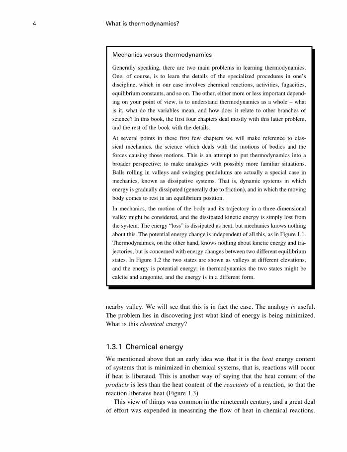
Mechanics versus thermodynamics
Generally speaking, there are two main problems in learning thermodynamics.
One, of course, is to learn the details of the specialized procedures in one’s
discipline, which in our case involves chemical reactions, activities, fugacities,
equilibrium constants, and so on. The other, either more or less important depend-
ing on your point of view, is to understand thermodynamics as a whole – what
is it, what do the variables mean, and how does it relate to other branches of
science? In this book, the first four chapters deal mostly with this latter problem,
and the rest of the book with the details.
At several points in these first few chapters we will make reference to clas-
sical mechanics, the science which deals with the motions of bodies and the
forces causing those motions. This is an attempt to put thermodynamics into a
broader perspective; to make analogies with possibly more familiar situations.
Balls rolling in valleys and swinging pendulums are actually a special case in
mechanics, known as dissipative systems. That is, dynamic systems in which
energy is gradually dissipated (generally due to friction), and in which the moving
body comes to rest in an equilibrium position.
In mechanics, the motion of the body and its trajectory in a three-dimensional
valley might be considered, and the dissipated kinetic energy is simply lost from
the system. The energy “loss” is dissipated as heat, but mechanics knows nothing
about this. The potential energy change is independent of all this, as in Figure 1.1.
Thermodynamics, on the other hand, knows nothing about kinetic energy and tra-
jectories, but is concerned with energy changes between two different equilibrium
states. In Figure 1.2 the two states are shown as valleys at different elevations,
and the energy is potential energy; in thermodynamics the two states might be
calcite and aragonite, and the energy is in a different form.
nearby valley. We will see that this is in fact the case. The analogy is useful.The problem lies in discovering just what kind of energy is being minimized.What is this chemical energy?
1.3.1 Chemical energy
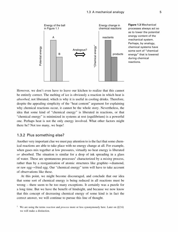
We mentioned above that an early idea was that it is the heat energy contentof systems that is minimized in chemical systems, that is, reactions will occurif heat is liberated. This is another way of saying that the heat content of theproducts is less than the heat content of the reactants of a reaction, so that thereaction liberates heat (Figure 1.3)
This view of things was common in the nineteenth century, and a great dealof effort was expended in measuring the flow of heat in chemical reactions.
1.3 A mechanical analogy 5
Energy of the ballin Figure 1.1
B
AP
oten
tial e
nerg
y
Analogous?
‘‘Che
mic
al e
nerg
y’’
reactants
products
Energy change inchemical reactions
Figure 1.3 Mechanicalprocesses always act soas to lower the potentialenergy content of themechanical system.Perhaps, by analogy,chemical systems havesome sort of “chemicalenergy” that is loweredduring chemicalreactions.
However, we don’t even have to leave our kitchen to realize that this cannotbe entirely correct. The melting of ice is obviously a reaction in which heat isabsorbed, not liberated, which is why it is useful in cooling drinks. Therefore,despite the appealing simplicity of the “heat content” argument for explainingwhy chemical reactions occur, it cannot be the whole story. Nevertheless, theidea that some kind of “chemical energy” is liberated in reactions, or that“chemical energy” is minimized in systems at rest (equilibrium) is a powerfulone. Perhaps heat is not the only energy involved. What other factors mightthere be? Not too many, we hope!
1.3.2 Plus something else?
Another very important clue we must pay attention to is the fact that some chem-ical reactions are able to take place with no energy change at all. For example,when gases mix together at low pressures, virtually no heat energy is liberatedor absorbed. The situation is similar for a drop of ink spreading in a glassof water. These are spontaneous processes1 characterized by a mixing process,rather than by a reorganization of atomic structures like graphite→diamond,or raw egg→fried egg. Our “chemical energy” term will have to take accountof observations like these.
At this point, we might become discouraged, and conclude that our ideathat some sort of chemical energy is being reduced in all reactions must bewrong – there seem to be too many exceptions. It certainly was a puzzle fora long time. But we have the benefit of hindsight, and because we now knowthat this concept of decreasing chemical energy of some kind is in fact thecorrect answer, we will continue to pursue this line of thought.
1 We are using the terms reaction and process more or less synonymously here. Later on (§2.6)we will make a distinction.
6 What is thermodynamics?
1.4 Limitations of the thermodynamic model
This book outlines the essential elements of a first understanding of chemicalthermodynamics, especially as applied to natural systems. However, it is usefulat the start to have some idea of the scope of our objective – just how useful isthis subject, and what are its limitations? It is at the same time very powerfuland very limited. With the concepts described here, you can predict the equilib-rium state for most chemical systems, and therefore the direction and amountof reaction that should occur, including the composition of all phases whenreaction has stopped. The operative word here is “should.” Our model consistsof comparing equilibrium states, one with another, and determining which ismore stable under the circumstances. We will not consider how fast the reac-tion will proceed, or how to tell if it will proceed at all. Many reactions that“should” occur do not occur, for various reasons. We will also say very littleabout what “actually” happens during these reactions – the specific interactionsof ions and molecules that result in the new arrangements or structures that aremore stable. In other words, our model will say virtually nothing about whyone arrangement is more stable than another or has less “chemical energy,”just that it does, and how to determine that it does.
These are serious limitations. Obviously, we will often need to know notonly if a reaction should occur but if it occurs, and at what rate. A great dealof effort has also been directed toward understanding the structures of crystalsand solutions, and of what happens during reactions, shedding much light onwhy things happen the way they do. However, these fields of study are notcompletely independent. The subject of this book is really a prerequisite forany more advanced understanding of chemical reactions, which is why everychemist, environmental scientist, biochemist, geochemist, soil scientist, and thelike, must be familiar with it.
But in a sense, the limitations of our subject are also a source of its strength.The concepts and procedures described here are so firmly established partlybecause they are independent of our understanding of why they work. The lawsof thermodynamics are distillations from our experience, not explanations, andthat goes for all the deductions from these laws, such as are described in thisbook. As a scientist dealing with problems in the real world, you need to knowthe subject described here. You need to know other things as well, but thissubject is so fundamental that virtually every scientist has it in some form inhis tool kit.
1.5 Summary
The fundamental problem addressed here is why things (specifically, chemicalreactions) happen the way they do. Why does ice melt and water freeze? Whydoes graphite turn into diamond, or vice versa? Taking a cue from the studyof simple mechanical systems, such as a ball rolling in a valley, we propose
1.5 Summary 7
that these reactions happen if some kind of energy is being reduced, much asthe ball rolls in order to reduce its potential energy. However, we quickly findthat this cannot be the whole story – some reactions occur with no decrease inenergy. We also note that whatever kind of energy is being reduced (we call it“chemical energy”), it is not simply heat energy.
For a given ball and valley (Figure 1.1), we need to know only one parameterto determine the potential energy of the ball (its height above the base level,or bottom of the valley). In our “chemical energy” analogy, we know thatthere must be at least one other parameter, to take care of those reactions thathave no energy change. Determining the parameters of our “chemical energy”analogy is at the heart of chemical thermodynamics.
2Defining our terms
2.1 Something is missing
We mentioned in Chapter 1 that an early idea for understanding chemicalreactions held that spontaneous reactions would always be accompanied by theloss of energy, because the reactants were at a higher energy level than theproducts, and they wanted to go “downhill.” This energy was usually thoughtto be in the form of heat, but this idea received a setback when it was foundthat some spontaneous reactions in fact absorb heat. Also, there are somereactions, such as the mixing of gases, where the energy change is virtuallyzero yet the processes proceed very strongly and are highly nonreversible.Obviously, something is missing. If the ball-in-valley analogy is right, that is,if reactions do proceed in the direction of decreasing chemical energy of somekind, something more than just heat is involved.
To learn more about chemical reactions, we have to become a bit moreprecise in our terminology and introduce some new concepts. In this chapter, wewill define certain kinds of systems, because we need to be careful about whatkinds of matter and energy transfers we are talking about; equilibrium states,the beginning and ending states for processes; state variables, the propertiesof systems that change during reactions; processes, the reactions themselves;and phases, the different types of matter within the systems. All these termsrefer in fact to our models of natural systems, but they are also used to referto things in real life. To be quite clear about thermodynamics, it is a good ideato keep the distinction in mind.
2.2 Systems
2.2.1 Real life systems
In real life, a system is any part of the universe that we wish to consider.If we are conducting an experiment in a beaker, then the contents of thebeaker is our system. For an astronomer calculating the properties of theplanet Pluto, the solar system might be the system. In considering geochemical,biological, or environmental problems here on Earth, the choice of system is
8
2.2 Systems 9
usually fairly obvious, and depends on the kind of problem in which you areinterested.
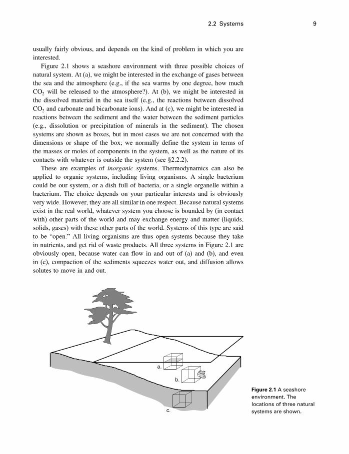
Figure 2.1 shows a seashore environment with three possible choices ofnatural system. At (a), we might be interested in the exchange of gases betweenthe sea and the atmosphere (e.g., if the sea warms by one degree, how muchCO2 will be released to the atmosphere?). At (b), we might be interested inthe dissolved material in the sea itself (e.g., the reactions between dissolvedCO2 and carbonate and bicarbonate ions). And at (c), we might be interested inreactions between the sediment and the water between the sediment particles(e.g., dissolution or precipitation of minerals in the sediment). The chosensystems are shown as boxes, but in most cases we are not concerned with thedimensions or shape of the box; we normally define the system in terms ofthe masses or moles of components in the system, as well as the nature of itscontacts with whatever is outside the system (see §2.2.2).
These are examples of inorganic systems. Thermodynamics can also beapplied to organic systems, including living organisms. A single bacteriumcould be our system, or a dish full of bacteria, or a single organelle within abacterium. The choice depends on your particular interests and is obviouslyvery wide. However, they are all similar in one respect. Because natural systemsexist in the real world, whatever system you choose is bounded by (in contactwith) other parts of the world and may exchange energy and matter (liquids,solids, gases) with these other parts of the world. Systems of this type are saidto be “open.” All living organisms are thus open systems because they takein nutrients, and get rid of waste products. All three systems in Figure 2.1 areobviously open, because water can flow in and out of (a) and (b), and evenin (c), compaction of the sediments squeezes water out, and diffusion allowssolutes to move in and out.
a.
b.
c.
Figure 2.1 A seashoreenvironment. Thelocations of three naturalsystems are shown.
10 Defining our terms
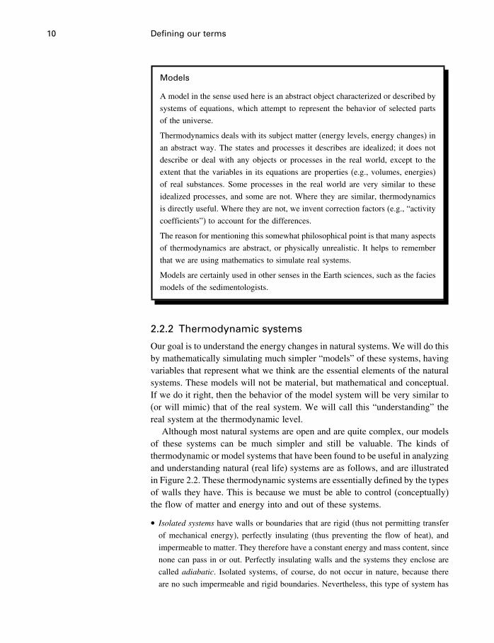
Models
A model in the sense used here is an abstract object characterized or described by
systems of equations, which attempt to represent the behavior of selected parts
of the universe.
Thermodynamics deals with its subject matter (energy levels, energy changes) in
an abstract way. The states and processes it describes are idealized; it does not
describe or deal with any objects or processes in the real world, except to the
extent that the variables in its equations are properties (e.g., volumes, energies)
of real substances. Some processes in the real world are very similar to these
idealized processes, and some are not. Where they are similar, thermodynamics
is directly useful. Where they are not, we invent correction factors (e.g., “activity
coefficients”) to account for the differences.
The reason for mentioning this somewhat philosophical point is that many aspects
of thermodynamics are abstract, or physically unrealistic. It helps to remember
that we are using mathematics to simulate real systems.
Models are certainly used in other senses in the Earth sciences, such as the facies
models of the sedimentologists.
2.2.2 Thermodynamic systems
Our goal is to understand the energy changes in natural systems. We will do thisby mathematically simulating much simpler “models” of these systems, havingvariables that represent what we think are the essential elements of the naturalsystems. These models will not be material, but mathematical and conceptual.If we do it right, then the behavior of the model system will be very similar to(or will mimic) that of the real system. We will call this “understanding” thereal system at the thermodynamic level.
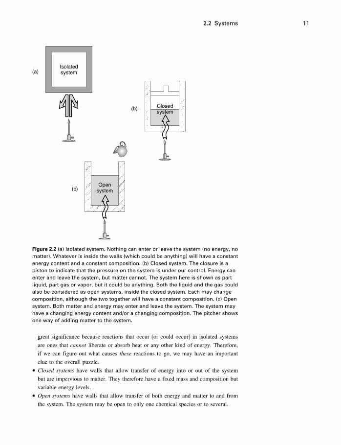
Although most natural systems are open and are quite complex, our modelsof these systems can be much simpler and still be valuable. The kinds ofthermodynamic or model systems that have been found to be useful in analyzingand understanding natural (real life) systems are as follows, and are illustratedin Figure 2.2. These thermodynamic systems are essentially defined by the typesof walls they have. This is because we must be able to control (conceptually)the flow of matter and energy into and out of these systems.
• Isolated systems have walls or boundaries that are rigid (thus not permitting transfer
of mechanical energy), perfectly insulating (thus preventing the flow of heat), and
impermeable to matter. They therefore have a constant energy and mass content, since
none can pass in or out. Perfectly insulating walls and the systems they enclose are
called adiabatic. Isolated systems, of course, do not occur in nature, because there
are no such impermeable and rigid boundaries. Nevertheless, this type of system has
2.2 Systems 11
Isolatedsystem
Opensystem
Closedsystem
(a)
(b)
(c)
Figure 2.2 (a) Isolated system. Nothing can enter or leave the system (no energy, nomatter). Whatever is inside the walls (which could be anything) will have a constantenergy content and a constant composition. (b) Closed system. The closure is apiston to indicate that the pressure on the system is under our control. Energy canenter and leave the system, but matter cannot. The system here is shown as partliquid, part gas or vapor, but it could be anything. Both the liquid and the gas couldalso be considered as open systems, inside the closed system. Each may changecomposition, although the two together will have a constant composition. (c) Opensystem. Both matter and energy may enter and leave the system. The system mayhave a changing energy content and/or a changing composition. The pitcher showsone way of adding matter to the system.
great significance because reactions that occur (or could occur) in isolated systems
are ones that cannot liberate or absorb heat or any other kind of energy. Therefore,
if we can figure out what causes these reactions to go, we may have an important
clue to the overall puzzle.• Closed systems have walls that allow transfer of energy into or out of the system
but are impervious to matter. They therefore have a fixed mass and composition but
variable energy levels.• Open systems have walls that allow transfer of both energy and matter to and from
the system. The system may be open to only one chemical species or to several.
12 Defining our terms
As mentioned above, most natural systems are open. However, it is possibleand convenient to model them as closed systems; that is, to consider a fixedcomposition, and simply ignore any possible changes in total composition. Ifwhat happens because of changes in composition is important, it can oftenbe handled by considering two or more closed systems of different composi-tions. Thus we will be dealing mostly with closed systems in our efforts tounderstand chemical reactions. Basically this means that we will be concernedmostly with individual chemical reactions, rather than with whole complexsystems. In other words, even though a bacterium is an open system, it canbe treated (modeled) as a closed system while considering many individualreactions within it. The reactants may need to be ingested and the productseliminated by the organism, but the reaction itself can be modeled indepen-dently of these processes. This greatly simplifies the task of understanding thebiochemical reactions. The same is true of most geochemical and environmentalsystems.
The most common kind of open system in chemical thermodynamics isrepresented in Figure 2.2b, that is, two open subsystems within an overall closedsystem. There can be any number of these “open subsystems,” and findingout how many there are and what their compositions are, given some physicalconditions, is a common problem in the application of thermodynamics. Wehave a brief look at other kinds of open systems in Chapter 4.
It is one of the paradoxes of thermodynamics that isolated systems, thathave no counterpart in the real world, are possibly the most important of all interms of our understanding of chemical reactions. You will have to wait untilChapter 4 to see why.
2.3 Equilibrium
In studying chemical reactions, we obviously need to know when they start andwhen they have ended. To do this, we define the state of equilibrium, when noreactions at all are proceeding. Here we encounter a distinct difference betweenreal and thermodynamic systems, because the state of equilibrium is defineddifferently in the two cases.
In thermodynamic systems, that is, in our models, equilibrium is definedin terms of chemical potentials, which we will get to in a later chapter. Thisstate, as you might imagine, is one of perfect equilibrium, perfect rest, withabsolutely no gradients or inhomogeneities of any kind. Real systems oftenapproach this state more or less closely, but probably never attain it. Whenreal systems do approach equilibrium, thermodynamics can be applied to them.Obviously, we need to have some way of telling whether real systems are “atequilibrium,” or have closely approached equilibrium.
2.3 Equilibrium 13
Equilibrium states in real systems have two attributes:
1. A real system at equilibrium has none of its properties changing with time, no matter
how long it is observed.
2. A real system at equilibrium will return to that state after being disturbed, that is,
after having one or more of its parameters slightly changed, then changed back to
the original values.
This definition is framed so as to be “operational,” that is, you can applythese criteria to real systems to determine whether they are at equilibrium. Andin fact, many real systems do satisfy the definition. For example, a crystal ofdiamond sitting on a museum shelf obviously has exactly the same propertiesthis year as last year (part 1 of the definition), and if we warm it slightlyand then put it back on the shelf, it will gradually resume exactly the sametemperature, dimensions, and so on that it had before we warmed it (part 2 ofthe definition). The same remarks hold for a crystal of graphite on the sameshelf, so that the definition can apparently be satisfied for various forms ofcarbon. Many other natural systems just as obviously are not at equilibrium.Any system having temperature, pressure, or compositional gradients will tendto change so as to eliminate these gradients, and is not at equilibrium until thathappens. A cup of hot coffee, for example, is not at equilibrium with the airaround it until it cools down.
So if diamond and graphite are both at equilibrium, do we have two kindsof equilibrium? In our ball-in-valley analogy, the ball in any valley would fitour definition. What distinction do we make between the lowest valley and theothers?
2.3.1 Stable and metastable equilibrium
In this section we use the simple mechanical analogy in §1.3 to distinguishbetween stable and metastable equilibrium. This explanation is satisfactory foran intuitive understanding, but we return to this subject for a better theoreticalunderstanding in §4.9.1.
Stable and metastable are the terms used to describe the system in its lowestequilibrium energy state and any other equilibrium energy state, respectively.In Figure 2.3, we see a ball on a surface having two valleys, one higher thanthe other. At (a), the ball is in an equilibrium position, that fulfills both parts ofour definition – it will stay there forever, and will return there if disturbed, aslong as the disturbance is not too great. However, it has not achieved the lowestpossible potential energy state, and therefore (a) is a metastable equilibriumposition. If the ball is pushed past position (b), it will roll down to the lowestavailable energy state at (d), a stable equilibrium state. During the fall, forexample, at position (c), the ball (system) is said to be unstable. In position (b),it is possible to imagine the ball balanced and unmoving, so that the first part
14 Defining our terms
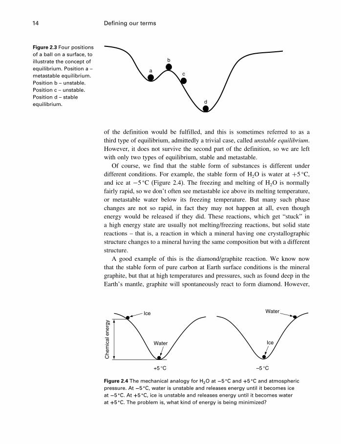
Figure 2.3 Four positionsof a ball on a surface, toillustrate the concept ofequilibrium. Position a –metastable equilibrium.Position b – unstable.Position c – unstable.Position d – stableequilibrium.
a
b
c
d
of the definition would be fulfilled, and this is sometimes referred to as athird type of equilibrium, admittedly a trivial case, called unstable equilibrium.However, it does not survive the second part of the definition, so we are leftwith only two types of equilibrium, stable and metastable.
Of course, we find that the stable form of substances is different underdifferent conditions. For example, the stable form of H2O is water at +5 �C,and ice at −5 �C (Figure 2.4). The freezing and melting of H2O is normallyfairly rapid, so we don’t often see metastable ice above its melting temperature,or metastable water below its freezing temperature. But many such phasechanges are not so rapid, in fact they may not happen at all, even thoughenergy would be released if they did. These reactions, which get “stuck” ina high energy state are usually not melting/freezing reactions, but solid statereactions – that is, a reaction in which a mineral having one crystallographicstructure changes to a mineral having the same composition but with a differentstructure.
A good example of this is the diamond/graphite reaction. We know nowthat the stable form of pure carbon at Earth surface conditions is the mineralgraphite, but that at high temperatures and pressures, such as found deep in theEarth’s mantle, graphite will spontaneously react to form diamond. However,
Che
mic
al e
nerg
y
Ice
Water Ice
Water
+5 °C –5 °C
Figure 2.4 The mechanical analogy for H2O at −5 �C and +5 �C and atmosphericpressure. At −5 �C, water is unstable and releases energy until it becomes iceat −5 �C. At +5 �C, ice is unstable and releases energy until it becomes waterat +5 �C. The problem is, what kind of energy is being minimized?
2.3 Equilibrium 15
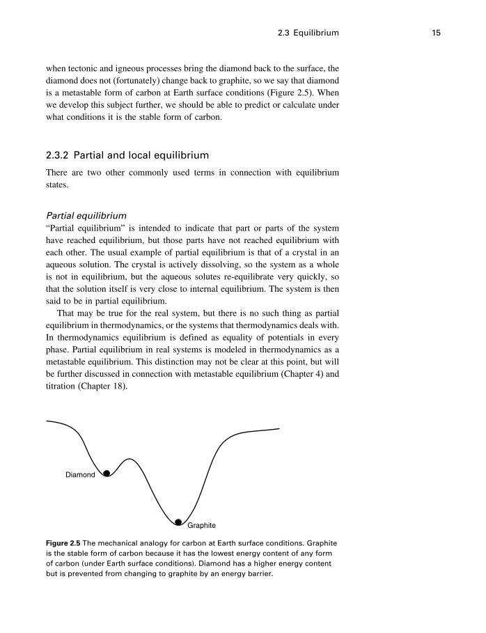
when tectonic and igneous processes bring the diamond back to the surface, thediamond does not (fortunately) change back to graphite, so we say that diamondis a metastable form of carbon at Earth surface conditions (Figure 2.5). Whenwe develop this subject further, we should be able to predict or calculate underwhat conditions it is the stable form of carbon.
2.3.2 Partial and local equilibrium
There are two other commonly used terms in connection with equilibriumstates.
Partial equilibrium“Partial equilibrium” is intended to indicate that part or parts of the systemhave reached equilibrium, but those parts have not reached equilibrium witheach other. The usual example of partial equilibrium is that of a crystal in anaqueous solution. The crystal is actively dissolving, so the system as a wholeis not in equilibrium, but the aqueous solutes re-equilibrate very quickly, sothat the solution itself is very close to internal equilibrium. The system is thensaid to be in partial equilibrium.
That may be true for the real system, but there is no such thing as partialequilibrium in thermodynamics, or the systems that thermodynamics deals with.In thermodynamics equilibrium is defined as equality of potentials in everyphase. Partial equilibrium in real systems is modeled in thermodynamics as ametastable equilibrium. This distinction may not be clear at this point, but willbe further discussed in connection with metastable equilibrium (Chapter 4) andtitration (Chapter 18).
Graphite
Diamond
Figure 2.5 The mechanical analogy for carbon at Earth surface conditions. Graphiteis the stable form of carbon because it has the lowest energy content of any formof carbon (under Earth surface conditions). Diamond has a higher energy contentbut is prevented from changing to graphite by an energy barrier.
16 Defining our terms
Local equilibriumReal world systems are in constant flux, and never really achieve thermo-dynamic equilibrium, but we want to apply thermodynamics to them anyway,so we have to choose parts of real systems which are reasonably close tothermodynamic equilibrium.
For example, you cannot apply thermodynamics to the ocean as a whole.Calcite is supersaturated at the surface, but undersaturated at 5 km depth(Chapter 16). Thermodynamics cannot be applied to a system which is bothsupersaturated and undersaturated. You can apply thermodynamics to volumesclose to equilibrium at the surface or at depth, not both together, so we say weapply thermodynamics to areas of “local equilibrium.” It is obviously importantto apply thermodynamics appropriately, and generally we do this, but the pointis that local equilibrium is not part of thermodynamics, it is a concept we need,a property that real systems must have, in order to apply thermodynamics.
Understanding thermodynamics does not depend in any way on local equi-librium, but applying it to natural systems does. The question then naturallyarises as to how one distinguishes between places having local equilibriumfrom places that do not. This question does not have a good answer. Placeshaving large gradients in temperature, pressure or composition can be ruled out,but how large is “large”? Quite often the practice is to apply thermodynamicsand see how it works out. If it seems to work well, then local equilibrium isassumed. Obviously some better approach would be desirable. There have beenseveral attempts at providing a quantitative criterion for local equilibrium. Themost accessible for Earth scientists appears to be that of Knapp (1989), whichis summarized in Zhu and Anderson (2002, Chapter 3), who also cite a numberof other references on the subject.
Defining local equilibrium
The question of fluid – solid phase equilibrium arises in many subject areas,including environmental problems, studies of diagenesis, long range flow insedimentary basins, ore genesis, magmatic – hydrothermal systems, regionalmetamorphism, and laboratory experimental systems. In each of these realsystems, local equilibrium in theory requires that any disequilibrium conditionrelax instantaneously to an equilibrium state. In reality, this relaxation occursover a finite time and, for a fluid-flow system, a finite distance. Knapp (1989)points out that each of these types of systems has a characteristic scale ofinterest, which is hundreds of meters or kilometers in studies of sedimentarybasins, but perhaps microns in studies of surface processes. If the problem isdefined on the kilometer scale, then disequilibrium over distances of centimetersis insignificant. The problem then is to determine, for a given system, the timerequired for a system in disequilibrium to reach equilibrium, and the distancethe fluid has moved in that time period.
2.4 State variables 17
Knapp considers the problem in terms of a one-dimensional flow path in aquartz sandstone. The moving water is initially at equilibrium with quartz, thena pulse of pure water is introduced, and the time and distance required for thereattainment of equilibrium are calculated. Quite a few factors are involved,including concentrations (including pH), temperature, fluid velocity, diffusionand dispersion coefficients, and of course kinetics, including the surface area(m2 of mineral per m3 of fluid). The results, presented in terms of Damköhlerand Peclet numbers,1 show that there is a region where the time and distance toequilibrium is reaction dominated, and there is another region where they aretransport or advection dominated. Local equilibrium can occur in both domains.Most natural environments with elevated temperatures fall in the reaction dom-inated domain, where the effects of dispersion and diffusion can safely beignored, but local equilibrium would appear to be a questionable approximationin what Knapp (1989) refers to as “human controlled environments” due tocharacteristically large fluid velocities and low temperatures.
This analysis by Knapp is useful in defining and clarifying the local equi-librium problem in a quantitative way. Unfortunately, despite the rather drasticsimplification, most of the parameters required to define the problem in realsituations at the present time are poorly known. The quantitative results arethen of questionable significance in any practical sense, but they are worthreflecting on. All applications of thermodynamics assume local equilibrium,but defining just what that is has proven difficult.
2.4 State variables
Systems at equilibrium have measurable properties. A property of a system isany quantity that has a fixed and invariable value in a system at equilibrium,such as temperature, density, or refractive index. Every system has dozens ofproperties. If the system changes from one equilibrium state to another, theproperties therefore have changes that depend only on the two states chosen,and not on the manner in which the system changed from one to the other.This dependence of properties on equilibrium states and not on processes isreflected in the alternative name for them, state variables. Several importantstate variables (which we consider in later chapters) are not measurable in theabsolute sense in a particular equilibrium state, though they do have fixed,finite values in these states. However, their changes between equilibrium statesare measurable.
1 The Damköhler number (Da) expresses the rate of reaction relative to the advection or fluidflow rate. A large Da value means that reaction is fast relative to transport and that aqueousconcentrations may change rapidly in time and space. The Peclet number (Pe) expresses theimportance of advection relative to dispersion in transporting aqueous compounds. A large Pevalue means that advection dominates, which may result in large concentration gradients; asmall Pe value suggests that dispersion dominates, which promotes mixing in the fluid phase.
18 Defining our terms
Reference in the above definition to “equilibrium states” rather than “stableequilibrium states” is deliberate, since as long as metastable equilibrium statesare truly unchanging they will have fixed values of the state variables. Thus bothdiamond and graphite have fixed properties. Metastable states are extremelycommon. For example, virtually all organic compounds are metastable in anoxidizing environment, such as the Earth’s atmosphere. We should be gratefulfor those “activation energy barriers” that prevent metastable states from spon-taneously changing to stable states; otherwise we would not be here to discussthe matter.
2.4.1 Total versus molar properties
Many physical properties, such as the volume and various energy terms, come intwo forms – the total quantity in the system and the quantity per mole orper gram of substance considered. We use different fonts for these total andmolar properties. For example, water has a volume per mole (V ) of about18.0686 cm3 mol−1, so if we have 30 moles of water in a beaker, its vol-ume (V) is 542.06 cm3. This relationship for a pure substance such as H2O isZ = Z/ni, where Z is any total property, Z is the corresponding molar prop-erty, and ni is the number of moles of the substance. In our water example,above, 542�06/30 = 18�068. In more complex systems where more than onesubstance is present, total and molar properties are related in the same way.A beaker containing, for example, a kilogram of water (55.51 moles H2O) and1 mole of NaCl occupies 1019.9 cm3. The molar volume of the system is thenZ = Z/
∑i ni, or 1019�9/�1+55�51�= 18�05 cm3 mol−1.
These two types of state variables have been given names:
• Extensive variables are proportional to the quantity of matter being considered – for
example, total volume (V).• Intensive variables are independent of the total size of the system and include concen-
tration, viscosity, and density, as well as all the molar properties, such as the molar
volume, V .
Scientific versus engineering units
In science, molar properties, such as molar volumes, molar energies, are most
commonly used. In engineering on the other hand, specific properties are more
common. Specific properties are mass-related rather than mole-related. Thus
the specific volume of water at 25 �C is 1.0029 cm3 g−1. Molar and specific
properties are of course related by the molar mass (or so-called gram formulas
weight, gfw) of the substance. That for water is 18.0153, so 1�0029cm3 g−1 ×18�0153gmol−1 = 18�068cm3 mol−1.
2.4 State variables 19
Of course, many equations look much the same with total and molar prop-erties because ratios are involved. That is, if ��U/�S�V = T , then it is alsotrue that ��U/�S�V = T ; or if ��G/�P�T = V, then ��G/�P�T = V , so that thedistinction may seem to be unimportant. However, sometimes it is important,as we will see. In general terms, we use the total form of our variables (boldtype) in some theoretical discussions, and the molar form (italic type) in mostcalculations.
Partial molar propertiesIn addition to total and molar properties, we have partial molar properties,which are a little trickier to understand. It’s relatively easy to see that thevolume (extensive variable) of a system depends on how much stuff you havein the system, but that its temperature or density (intensive variables) do not.This is true no matter how many different phases there are in the system, aslong as you are considering the whole system, not just parts of it.
A problem arises, though, when you consider the properties of solutions,which can have variable concentrations of solutes. The volume per gram ofhalite, NaCl, is the same whether you consider 10 or 20 grams of it. But whatis the volume per gram of 10 grams of NaCl dissolved in a liter of water?This property depends on the concentration of NaCl – the volume per gram orper mole of 20 dissolved grams is different from that of 10 dissolved grams.And what is the volume of something dissolved in something else? How is itdefined, or measured? These are important questions, and will be discussed inChapter 10.
The properties of dissolved substances is discussed in terms of partial molarproperties, the formal definition of which is
Zi =(�Z�ni
)T�P�ni
(2.1)
where Z is the total or extensive form of any thermodynamic parameter, Zthe partial molar form, ni is the number of moles of component i, and ni isthe number of moles of all components other than i in the same solution. Noteparticularly that the partial derivative is taken of the total quantity Z, not themolar Z, and that the main constraints are T and P. However, the importantthing to know about partial molar properties is not this differential equation, butthat they are the properties per mole of substances at a particular concentrationin a particular solution, as explained in Chapter 10. You think about partialmolar properties in exactly the same way you think about molar properties.The only difference is that for a given substance, they are not fixed quantitiesat a given T and P, but vary with the concentration of the substance and thenature of the solution.
The differences between total, molar, and partial molar properties is alsodiscussed in more mathematical terms in Appendix C.
20 Defining our terms
2.5 Phases and components
We must also have terms for the various types of matter to be found withinour thermodynamic systems. A phase is defined as a homogeneous body ofmatter, having distinct boundaries with adjacent phases, and so is mechanicallyseparable from the other phases. The shape, orientation, and position of thephase with respect to other phases are irrelevant, so that a single phase mayoccur in many places in a system. Thus the quartz in a granite is a single phase,regardless of how many grains of quartz there are. A salt solution is a singlephase, as is a mixture of gases. There are only three very common types ofphases – solid, liquid, and gas or vapor. A system having only a single phaseis said to be homogeneous, and multiphase systems are heterogeneous.
The term generally used to describe the chemical composition of a systemis component. The components of a system are defined by the smallest set ofchemical formulas required to describe the composition of all the phases in thesystem. This simple definition is sometimes surprisingly difficult to use. Totake a simple example, consider a solution of salt (NaCl) in water (H2O), inequilibrium with water vapor. This might look like Figure 2.2b. There are twophases, liquid and vapor, and two components, NaCl and H2O. A chemicalanalysis could report the amounts or concentrations of Na, Cl, H, and O in thesystem, but only two chemical formulas are needed to describe the compositionsof both phases.
Unfortunately, this does not nearly encompass all we need to say about com-ponents. We will have more to say in Chapter 11, but we should at least pointout that the definition of components given above (“smallest set of chemicalformulas…”) is used for phases in our models, not in real systems. For exam-ple, analysis of any calcite crystal will reveal the presence of many elementsbesides those in the formulas CaCO3. Nevertheless, component CaCO3 is veryoften used to represent calcite, whatever its actual composition.
2.5.1 Real versus model systems
Equilibrium, phases, and components are terms that appear to apply toreal systems, not just to the model systems that we said thermodynamicsapplies to, and in general conversation, they do. But real phases, especiallysolids, are never perfectly homogeneous. And real systems don’t really havecomponents, only our models of them do. Seawater, for example, has anincredibly complex composition, containing dozens of elements. But our ther-modynamic models might model seawater as having two, three, or more com-ponents, depending on the application. As for equilibrium, real systems dooften achieve equilibrium as we have defined it, but it is never a perfectequilibrium.
However, the fact that real phases are more or less homogeneous, andthat real systems achieve an approximate equilibrium, is what makes thermo-dynamics useful. The model is perfect, but real life comes close enough in
2.6 Processes 21
many respects so that the model is useful. In fact, the close similarity betweenreality and our models of reality, and the fact that we use the same terms todescribe each, may lead to a certain degree of confusion as to what we aretalking about. Usually no harm is done, and the distinction gets easier withpractice.
2.6 Processes
Finally, we get to something that looks more interesting. Processes arewhat we are usually interested in – changes in the real world. In geology,these might be igneous, diagenetic, or metamorphic processes. In biology,they might be cellular processes. In the environmental world, they might bepotentially harmful processes near waste disposal sites – the possibilities areendless. However, most of the processes of interest to us have one thingin common – they are extremely complicated. The only hope we have ofunderstanding them is to break complex processes down into their simplercomponent parts, and to construct simplified models of them. We have alreadybegun to do this by defining several types of simple systems that we canuse; we will now define a process in a way that will help us model realprocesses.
A thermodynamic process is what happens when a system changes fromone equilibrium state to another. Thus any two equilibrium states of the systemmay be connected by an infinite number of different processes because onlythe initial and final states are fixed; anything at all could happen during theact of changing between them. A chemical reaction is one kind of process, butthere are others. For example, simply warming or cooling a system is a processaccording to our definition.
In spite of there seeming to be an endless number of kinds of processesin the world, we find that in thermodynamic models there are only two –reversible and irreversible.2
• The most important irreversible processes are those that begin in a metastable equi-
librium state and lead to a more stable state, such as aragonite recrystallizing to
calcite. Another kind would be a stable equilibrium state changing to a lower energy
stable equilibrium state, such as when the weight on a piston is replaced by a smaller
weight.• Processes that begin in a stable equilibrium state and proceed to another stable equi-
librium state, without ever leaving the state of equilibrium more than infinitesimally,
are reversible processes.
2 In some treatments of thermodynamics there is a third type – the virtual process. See Reiss(1965) for its use.
22 Defining our terms
2.6.1 Irreversible processes
We have defined a metastable state of a system as a state that has more thanthe minimum energy for the given conditions, but is for some reason preventedfrom releasing that energy and reacting or changing to the stable state ofminimum energy. An irreversible process is one that occurs when whateverconstraint is holding the system in its high energy state is removed, and thesystem slides down the energy gradient to a lower energy state. We considerconstraints in more detail in Chapter 4.
The only example we have given thus far of a metastable system is themineral diamond, that could lower its energy content by changing into graphitebut does not, because energy is required to break the carbon–carbon bonds indiamond (which are very strong) before the atoms can rearrange themselvesinto the graphite structure. There are many other similar examples of metastableminerals. We have also mentioned that most organic compounds, such as all theones in living organisms, are metastable. When the life processes maintainingtheir existence cease, they quickly react (decompose) to form more stablecompounds.
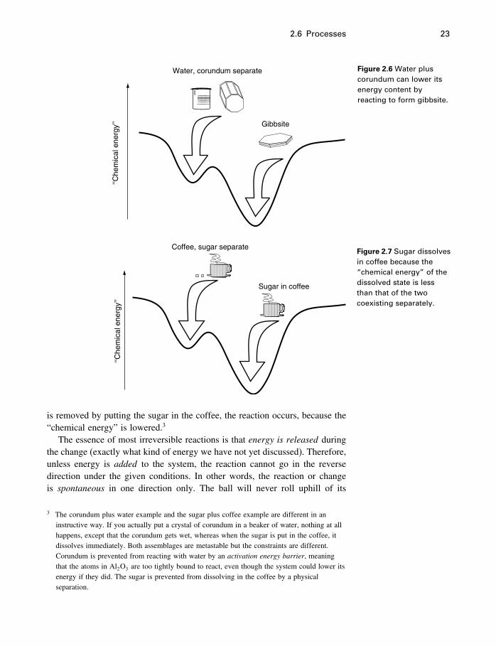
In most of the chemical reactions we will be considering, a combinationof minerals, or minerals plus liquids or gases, reacts to form some differentminerals under some given conditions. For example, the mineral corundum(Al2O3) is stable, considered by itself (i.e., there is no other form of Al2O3
that is more stable), but in the presence of water it reacts to form gibbsite(Al2O3 ·3H2O). The reaction is
Al2O3�s�+3H2O�l�= Al2O3 ·3H2O�s� (2.2)
and the energy relationships are shown in Figure 2.6. We will use �s�, �l�, �g�,and �aq� after our formulas to indicate whether they are in the solid, liquid,gas, or aqueous (dissolved in water) state.
Do not confuse the metastability of diamond at Earth surface conditionswith the metastability of corundum or water. Diamond is metastable becausethe same carbon atoms would have a lower energy in the crystal structure ofgraphite. But corundum by itself is not metastable, and neither is water, at25 �C and atmospheric pressure. It is the combination of corundum and waterthat can be regarded as metastable, because their combined atoms would havea lower energy level in the form of gibbsite.
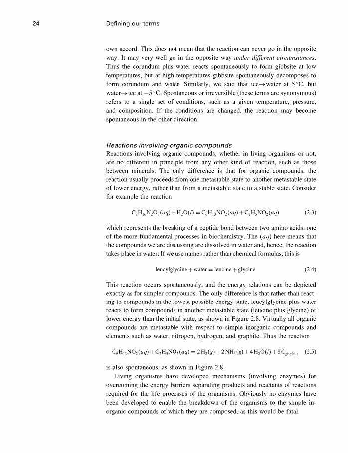
Another example is the dissolution of sugar in coffee (Figure 2.7), for whichwe cannot write a simple balanced reaction. Nevertheless, the assemblage ofsugar lumps and a cup of coffee is a metastable assemblage in our usage.They are prevented from reacting (sugar dissolving) by the fact that they areseparated, which constitutes a constraint on the system. When the constraint
2.6 Processes 23
Water, corundum separate
Gibbsite‘‘C
hem
ical
ene
rgy’
’
Figure 2.6 Water pluscorundum can lower itsenergy content byreacting to form gibbsite.
Figure 2.7 Sugar dissolvesin coffee because the“chemical energy” of thedissolved state is lessthan that of the twocoexisting separately.
Coffee, sugar separate
‘‘Che
mic
al e
nerg
y’’
Sugar in coffee
is removed by putting the sugar in the coffee, the reaction occurs, because the“chemical energy” is lowered.3
The essence of most irreversible reactions is that energy is released duringthe change (exactly what kind of energy we have not yet discussed). Therefore,unless energy is added to the system, the reaction cannot go in the reversedirection under the given conditions. In other words, the reaction or changeis spontaneous in one direction only. The ball will never roll uphill of its
3 The corundum plus water example and the sugar plus coffee example are different in aninstructive way. If you actually put a crystal of corundum in a beaker of water, nothing at allhappens, except that the corundum gets wet, whereas when the sugar is put in the coffee, itdissolves immediately. Both assemblages are metastable but the constraints are different.Corundum is prevented from reacting with water by an activation energy barrier, meaningthat the atoms in Al2O3 are too tightly bound to react, even though the system could lower itsenergy if they did. The sugar is prevented from dissolving in the coffee by a physicalseparation.
24 Defining our terms
own accord. This does not mean that the reaction can never go in the oppositeway. It may very well go in the opposite way under different circumstances.Thus the corundum plus water reacts spontaneously to form gibbsite at lowtemperatures, but at high temperatures gibbsite spontaneously decomposes toform corundum and water. Similarly, we said that ice→water at 5 �C, butwater→ice at −5 �C. Spontaneous or irreversible (these terms are synonymous)refers to a single set of conditions, such as a given temperature, pressure,and composition. If the conditions are changed, the reaction may becomespontaneous in the other direction.
Reactions involving organic compoundsReactions involving organic compounds, whether in living organisms or not,are no different in principle from any other kind of reaction, such as thosebetween minerals. The only difference is that for organic compounds, thereaction usually proceeds from one metastable state to another metastable stateof lower energy, rather than from a metastable state to a stable state. Considerfor example the reaction
C8H16N2O3�aq�+H2O�l�= C6H13NO2�aq�+C2H5NO2�aq� (2.3)
which represents the breaking of a peptide bond between two amino acids, oneof the more fundamental processes in biochemistry. The �aq� here means thatthe compounds we are discussing are dissolved in water and, hence, the reactiontakes place in water. If we use names rather than chemical formulas, this is
leucylglycine+water = leucine+glycine (2.4)
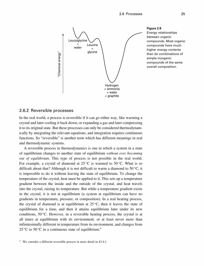
This reaction occurs spontaneously, and the energy relations can be depictedexactly as for simpler compounds. The only difference is that rather than react-ing to compounds in the lowest possible energy state, leucylglycine plus waterreacts to form compounds in another metastable state (leucine plus glycine) oflower energy than the initial state, as shown in Figure 2.8. Virtually all organiccompounds are metastable with respect to simple inorganic compounds andelements such as water, nitrogen, hydrogen, and graphite. Thus the reaction
C6H13NO2�aq�+C2H5NO2�aq�= 2H2�g�+2NH3�g�+4H2O�l�+8Cgraphite (2.5)
is also spontaneous, as shown in Figure 2.8.Living organisms have developed mechanisms (involving enzymes) for
overcoming the energy barriers separating products and reactants of reactionsrequired for the life processes of the organisms. Obviously no enzymes havebeen developed to enable the breakdown of the organisms to the simple in-organic compounds of which they are composed, as this would be fatal.
2.6 Processes 25
Figure 2.8Energy relationshipsbetween organiccompounds. Most organiccompounds have muchhigher energy contentsthan do combinations ofsimple inorganiccompounds of the sameoverall composition.
‘‘Che
mic
al e
nerg
y’’
Leucylglycine+
waterLeucine
+glycine
Hydrogen+ ammonia
+ water+ graphite
2.6.2 Reversible processes
In the real world, a process is reversible if it can go either way, like warming acrystal and later cooling it back down, or expanding a gas and later compressingit to its original state. But these processes can only be considered thermodynam-ically by integrating the relevant equations, and integration requires continuousfunctions. So “reversible” is another term which has different meanings in realand thermodynamic systems.
A reversible process in thermodynamics is one in which a system in a stateof equilibrium changes to another state of equilibrium without ever becomingout of equilibrium. This type of process is not possible in the real world.For example, a crystal of diamond at 25 �C is warmed to 50 �C. What is sodifficult about that? Although it is not difficult to warm a diamond to 50 �C, itis impossible to do it without leaving the state of equilibrium. To change thetemperature of the crystal, heat must be applied to it. This sets up a temperaturegradient between the inside and the outside of the crystal, and heat travelsinto the crystal, raising its temperature. But while a temperature gradient existsin the crystal, it is not at equilibrium (a system at equilibrium can have nogradients in temperature, pressure, or composition). In a real heating process,the crystal of diamond is at equilibrium at 25 �C, then it leaves the state ofequilibrium for a time, and then it attains equilibrium later under its newconditions, 50 �C. However, in a reversible heating process, the crystal is atall times at equilibrium with its environment, or at least never more thaninfinitesimally different in temperature from its environment, and changes from25 �C to 50 �C in a continuous state of equilibrium.4
4 We consider a different reversible process in more detail in §3.4.1.
26 Defining our terms
The reversible process as defined is impossible in the real world. However,it is quite simple in the thermodynamic model, because the temperature, vol-ume, and all other properties of the diamond are just points on mathematicalsurfaces in the model, and there is nothing to prevent the point representing thetemperature to move around on a surface representing the equilibrium valuesof various properties of the diamond.
Why in the world would we be interested in such a strange kind of impossi-ble process? It’s simple, really. The reason the reversible process (defined as acontinuous succession of equilibrium states) is important in the thermodynamicmodel is that it is the only kind of process that our mathematical tools of dif-ferentiation and integration can be applied to – they only work on continuousfunctions. Once our crystal of diamond leaves its state of equilibrium at 25 �C,practically anything could happen to it, but as long as it settles back to equi-librium at 50 �C, all of its state variables have changed by fixed amounts fromtheir values at 25 �C. We have equations to calculate these energy differences,but they refer to lines and surfaces in our model, and that means that they mustrefer to continuous equilibrium between the two states.
In other words, to calculate the energy difference between the two states,we must use a fictitious path (the reversible process) between the two states.The result is the real energy difference, no matter what actually happened tothe system between the two states. The reversible process is another exampleof the difference between the real world and our models of the real world.Reversible processes are quite simple to carry out in our models, because themodels are mathematical, not real.
2.6.3 Egg reactions
We have not discussed all the examples we used in Chapter 1. To concludeour discussion of various common chemical reactions (§1.2.1), we shoulddiscuss the thermodynamics of frying eggs. At a simple level, we could saythat the egg in the refrigerator represents a metastable state, and that frying itpromotes a reaction to a more stable state, analogous to the leucylglycine +water→leucine + glycine reaction in Figure 2.8. Even if this was the case,putting the fried egg back in the refrigerator would not suffice to reverse thereaction; going from a stable state to a metastable one requires a source ofenergy – it won’t occur spontaneously. In the water/ice case, the water returnsto ice in the fridge because ice is the stable form there.
Strictly speaking, however, we know that eggs in the refrigerator won’t lastindefinitely; they will eventually “go bad.” This means that they are not ina truly metastable state in the refrigerator, but an unstable, slowly changingstate. This means that because the raw egg occupies no “valley” for the eggcomponents to roll into, it is very unlikely that we could restore the raw eggstate, even if we had an energy source.

2.6 Processes 27
In studying natural systems, such as eggs, it is often quite difficult todistinguish stable, metastable, and unstable states from each other without aconsiderable amount of work and ingenuity, but it can be done. When youget numbers from tables, as we will be doing, all this work has been donefor you, although you have to realize that because of the difficulties involved,some of the data may not be accurate and may be revised at some future date.A compound believed to be stable under given conditions may later be foundto be metastable after more careful work is done.
Reactions in these complex systems are actually made up of a number ofsimpler reactions, and applying thermodynamics requires that the individualreactions be treated separately. The individual biochemical reactions in manyorganic systems still have not been figured out. Nevertheless, we are confi-dent that any particular reaction, once defined, will follow the logic and thesystematics described in this book.
2.6.4 Notation
Reaction deltasWe have now set up the general framework within which thermodynamics isable to deal with processes. Any given process or chemical reaction withina chosen system will proceed from an initial equilibrium state (normally ametastable equilibrium state) to another equilibrium state more stable than thefirst one. During this process or reaction the system is out of equilibrium.The system has a number of properties or state variables, such as volume andenergy content, that have fixed values in equilibrium states and that thereforehave fixed amounts of change between equilibrium states. These changes arealways written using a delta notation, where the delta refers to the property inthe final state minus the property in the initial state. For example, if the systemundergoes a process during which its (molar) volume (V ) changes from Vinitialto Vfinal, we write
�V = Vfinal−Vinitial (2.6)
If the process is a chemical reaction, a number of compounds may beinvolved. A generalized chemical reaction could be written as
aA+bB+· · · =mM+nN+· · ·
An example is Equation (2.2), where A is Al2O3, B is H2O, and M isAl2O3 ·3H2O (there is no N); a and m are 1 and b is 3. The quantities A, B, M,and N are chemical formulas representing any compounds or elements we hap-pen to be interested in, and each can be solid, liquid, gas, or a solute. One sideof the reaction will usually be more stable than the other, and a reaction willtend to occur, unless there is an energy barrier preventing the reaction, or unless
28 Defining our terms
the compounds are all at equilibrium together. In this case, the volume changeduring the reaction is �rV (we insert a subscript “r” to indicate a chemicalreaction) and is equal to the sum of the volumes of the reaction products (thefinal state) minus the sum of the volumes of the reactants (the initial state). Thus
�rV =mVM+nVN+· · ·−aVA−bVB−· · ·
where VM is the volume of a mole of compound M, and so on. For example,the change in volume for reaction (2.2) is
�rV = VAl2O3·3H2O−VAl2O3
−3VH2O(2.7)
Note that each volume must be multiplied by its corresponding stoichiometriccoefficient in the reaction. Molar volumes are readily available for most puresubstances.
Following this convention, the change in energy of the ball rolling downthe hill in Figure 1.1 would be a negative quantity, as shown in Figure 1.3(energy in state B minus energy in state A is negative). It follows, then, thatthe change in the “chemical energy” term we are looking for will always be anegative quantity in spontaneous reactions, as also shown in Figure 1.3 (energyof products minus energy of reactants).
Chemical equationsFor the most part, when we write reactions such as (2.2) and (2.3), we usethe = sign to indicate only that the reaction is “balanced,” meaning that thesame number and kinds of atoms appear on both sides, and that any electricalcharges are also the same on both sides. If we want to emphasize that thereaction proceeds strongly or irreversibly we may use an arrow, as in A→ B,and if we want to emphasize that the two sides are in equilibrium, we mightuse A� B. However, the = sign includes these possibilities, and all others.
2.7 Summary
If you look around the physical world today, you realize that there is anincredible number of chemical and physical processes going on all around you,and as you look into these in more and more detail, as science has done, youfind more and more complexity at all levels, right down to the atomic andsubatomic levels. How can we systematize and understand these processes insuch a way as to be able to control some of them for our own purposes?
Thermodynamics is the net result of our attempts to do this. It is not adescription of any real process but a rather abstract model that can be usedfor all real processes. Processes in the real world are incredibly complex, butour models of them are quite simple, containing a number of carefully definedconcepts. Processes (reactions, changes) involve energy and/or mass changes,
2.7 Summary 29
and these must enter or leave the place where the process is occurring; sothermodynamics begins by defining several types of systems, depending on howthe energy and/or mass is transferred. Processes must be defined by beginningand ending states, so thermodynamics defines equilibrium states, some havingmore energy (metastable equilibrium states) than others (stable equilibriumstates), and processes or reactions that are able to go from higher energy statesto lower energy states (irreversible processes), just like a ball rolling down ahill. Of course, a state of lower energy (stable) under one set of conditions
Volume change
The volume data in Appendix B are listed under V �, where superscript� means
standard state conditions, which we will discuss later. In the corundum – gibbsite
reaction, then,
�rV� = V �
Al2O3·3H2O−V �
Al2O3−3V �
H2O(2.8)
= 63�912−25�575−3×18�068
=−15�867cm3 mol−1
There is therefore a net decrease in volume of−15�867cm3 mol−1 for the reaction
as written. But you could equally well write
�rV� = 1
3V�Al2O3·3H2O
− 13V
�Al2O3
−V �H2O
(2.9)
=−5�289cm3 mol−1
Or you could write
�rV� = 2V �
Al2O3·3H2O−2V �
Al2O3−6V �
H2O(2.10)
=−31�734cm3 mol−1
All these results are cm3 per mole, so the question is, per mole of what?
Clearly, the meaning of �rV� in this simple case is the volume change per mole
of whatever species have a stoichiometric coefficient of 1.0. The volume change
is −15�867cm3 per mole of Al2O3 consumed or Al2O3 · 3H2O formed (Equa-
tion 2.2; 2.8), and −5�289cm3 per mole of H2O consumed (Equation 2.9). How-
ever, a mole of Al2O3 or H2O need not be consumed, conceptually or in reality.
The cm3 mol−1 unit is actually a rate term, and as MacDonald (1990) points out,
just as a car does not need to travel for an hour for its speed to be 100 kmhour−1,
a mole of reaction need not occur for its �rV� to be −15�867cm3 mol−1.
We make another small point about delta notation after introducing the affinity
in Chapter 18 (page 567).
30 Defining our terms
may be a state of higher energy (metastable) under other conditions (diamondis metastable at the Earth’s surface, but stable deep in the mantle). Corundumand water are, by themselves, perfectly stable and unreactive, but together theyhave a higher energy state than does gibbsite.
The only thermodynamic difference between organic reactions (includingthose in living organisms) and inorganic reactions is that both the reactants andproducts of organic reactions are invariably metastable compounds; metastable,that is, with respect to simple inorganic compounds and elements. Inorganicreactions may involve metastable compounds, but more frequently they involvea metastable assemblage changing to a stable one (one having the lowestpossible energy state).
Therefore, the determination of the energy states of substances and howthey change under changing conditions is fundamental to understanding whatprocesses are possible, and why they happen. The determination of the energystates of individual substances must be done by experiment and measurement,not by theoretical calculation, and the results are available in tables of data likethose at the end of this book. Calculation of the change of these energy termswith changing conditions can be carried out only for hypothetical reversibleprocesses, that are not possible in reality but are quite simple in the thermody-namic model.
As for the energy barriers that often prevent reactions from occurring,thermodynamics has nothing whatever to say about them. It pretends theydo not exist. More exactly, thermodynamics simply deals with energy levels,energy differences. It does not concern itself with whether a system actuallylowers its energy level or not. This is an important omission, of course, and isthe subject of much study in other branches of science, particularly kinetics.
The most important question now is what kind of energy is released duringthese reactions? If it is not heat energy, then what is it? We have called it“chemical energy,” but this is just because we haven’t said yet what it reallyis. This is the topic of the next two chapters.
3The first law of thermodynamics
3.1 Temperature and pressure scales
3.1.1 Temperature
One of the early triumphs of the study of thermodynamics was the demon-stration that there is an absolute zero of temperature. However, there areseveral different temperature scales, for historical reasons. All you need toknow about this is that the kelvin scale (named after William Thompson, LordKelvin) has an absolute zero of 0K1 and a temperature of 273.16K at thetriple point where water, ice, and water vapor are at equilibrium together. Themelting point of ice at one atmosphere pressure is 0.01 degrees less than this,at 273.15K (Figure 3.1). The Celsius scale (named after Anders Celsius, aSwedish astronomer) has a temperature of 0 �C at the ice point (273.15K) andabsolute zero at −273�15 �C. This gives almost exactly 100 �C between thefreezing and boiling points of water at one atmosphere, so water boils at 100 �C(373.15K). Thus the numerical conversion between the two scales is
T K = T �C+273�15
Remember that all equations in thermodynamics use the absolute or kelvintemperature scale, so that if you are given temperatures in �C, you must convertthem to the kelvin scale before using them. The “standard” temperature of25 �C for example is 298.15K.
3.1.2 Pressure
Force is measured in newtons (N), where 1 newton will give a mass of 1 kgan acceleration of 1 m sec−2. Pressure is defined as force per unit area, anda pressure of 1 newton per square meter (1 Nm−2) is called 1 pascal (1 Pa).This is a very small pressure, and older, larger pressure units are still in use.
1 It is not a point of major importance, but by international agreement, temperatures on thekelvin scale are so many “kelvins,” not “degrees kelvin,” while on the Celsius scale (no longercalled the centigrade scale) temperatures are “degrees Celsius.”
31
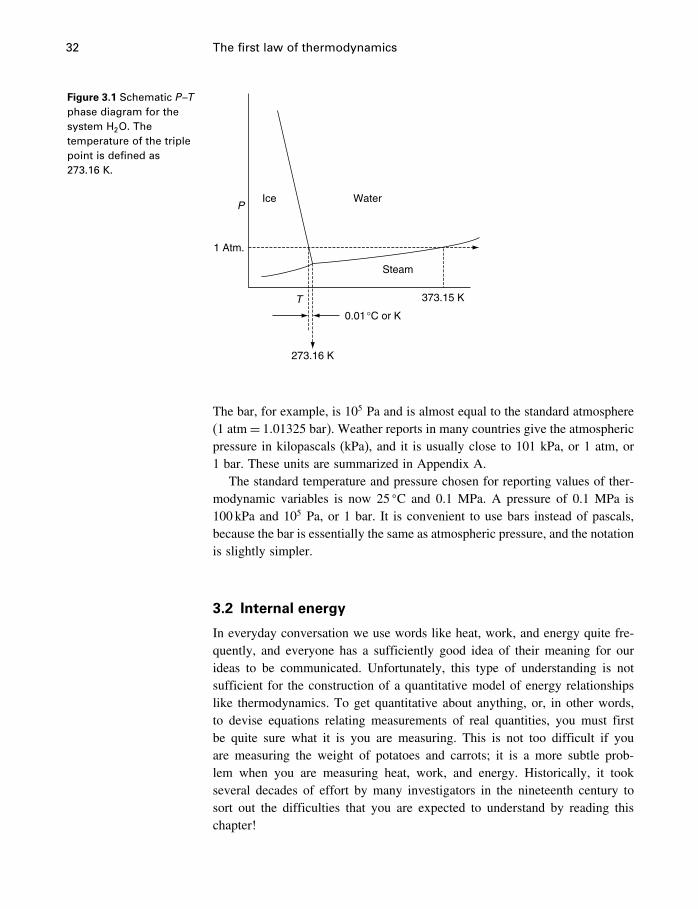
32 The first law of thermodynamics
Figure 3.1 Schematic P –Tphase diagram for thesystem H2O. Thetemperature of the triplepoint is defined as273.16 K.
Ice WaterP
1 Atm.
Steam
T
0.01°C or K
273.16 K
373.15 K
The bar, for example, is 105 Pa and is almost equal to the standard atmosphere(1 atm= 1�01325 bar). Weather reports in many countries give the atmosphericpressure in kilopascals (kPa), and it is usually close to 101 kPa, or 1 atm, or1 bar. These units are summarized in Appendix A.
The standard temperature and pressure chosen for reporting values of ther-modynamic variables is now 25 �C and 0.1 MPa. A pressure of 0.1 MPa is100 kPa and 105 Pa, or 1 bar. It is convenient to use bars instead of pascals,because the bar is essentially the same as atmospheric pressure, and the notationis slightly simpler.
3.2 Internal energy
In everyday conversation we use words like heat, work, and energy quite fre-quently, and everyone has a sufficiently good idea of their meaning for ourideas to be communicated. Unfortunately, this type of understanding is notsufficient for the construction of a quantitative model of energy relationshipslike thermodynamics. To get quantitative about anything, or, in other words,to devise equations relating measurements of real quantities, you must firstbe quite sure what it is you are measuring. This is not too difficult if youare measuring the weight of potatoes and carrots; it is a more subtle prob-lem when you are measuring heat, work, and energy. Historically, it tookseveral decades of effort by many investigators in the nineteenth century tosort out the difficulties that you are expected to understand by reading thischapter!
3.2 Internal energy 33
3.2.1 Energy
Everyone knows what energy is, but it is an elusive topic if you are lookingfor a deep understanding. In fact, a Nobel Prize-winning physicist has affirmedthat
It is important to realize that in physics today, we have no knowledge of what
energy is. (Feynman et al., 1963, pp. 4–2)
One of the most eminent of French scientists said
As we cannot give a general definition of energy, the principle of the
conservation of energy simply signifies that there is something which remains
constant. (Poincaré, 1952, p. 166)
If you consult a dictionary as to the meaning of energy, you find that thescientific meaning is ‘the ability to do work, i.e., move a body.’ In physics,work is not what you do from 9 to 5 every day, but the action of a forcemoving through a distance. So if you lift a book from the floor and put it onthe table, you are performing work (the mass of the book (multiplied by theacceleration due to gravity) times the distance from the floor to the table), andwe say that we expended energy to lift the book. It has proved tremendouslyuseful to take the view that the energy we expended has not disappeared, buthas been transferred to the book. In other words, the book on the table hasmore energy (potential energy) than it had on the floor, and the increase isexactly equal to the work we did in lifting it. Thus we can use energy to dowork, and we can do work on a system to increase the energy of that system.Work and energy are thus very closely related concepts (note that they havethe same dimensions in Appendix A).
If only things were that simple. However, we know that they are not, becausethe energy in a stick of dynamite on the table is not equal to the work expendedin lifting it from the floor. Similarly, the energy in water is not the same as inice, whether on the floor or the table. These complications are actually of twotypes.
1. There are many ways of doing work, because there are many kinds of forces. We
are particularly concerned with the work involved in chemical reactions.
2. The second is that although work and energy are indeed closely related, doing work
is not the only way of changing the energy of something, and changing the energy of
something does not always produce work. For example, we could change the energy
in our book by warming or cooling it.
We have to consider both work (in all its forms) and heat to get a consis-tent picture of energy changes. You will notice that although we have beenillustrating energy and work by using the ball-in-valley idea (Chapter 2) andthe book-and-table idea (this chapter), which emphasizes potential energy, this
34 The first law of thermodynamics
particular kind of energy/work is actually irrelevant in thermodynamics, exceptas an analogy. We will define the energy content of systems of importance tous to be the same whether they are on the floor or the table.
3.2.2 Absolute energy
In discussing energy, we always seem to be talking about changes in energy.The book has more energy on the table than on the floor, and presumablymore energy on the roof than on the table. And we add energy by warmingthe book, too. But how much energy has the book got in any particular state –say, on the table at 25 �C? What is the absolute energy content of the book?This was a difficult question until 1905, when Einstein postulated the essentialequivalence of mass and energy in his famous equation
Er =mc2
where Er is the rest energy of a system, m is the mass, and c is the speed oflight. Therefore, the energy contained in any macroscopic system is extremelylarge, and adding energy to a system (for instance by heating it) will in factincrease its mass. However, ordinary (i.e., nonnuclear) energy changes result inextremely small and unmeasurable changes in mass, so that relativity theory isnot very useful to us, except in the sense that it gives energy an absolute kindof meaning, which is sometimes helpful in trying to visualize what energy is.
Thus in considering ordinary everyday kinds of changes and chemical reac-tions, we will continue to deal with energy changes only, never with how muchenergy is in any particular equilibrium state. This is entirely sufficient for ourneeds, but it does introduce some complications that would be avoided if wehad a useful absolute energy scale.
3.2.3 The internal energy
All that is required to develop our model of energy relationships is that everyequilibrium state of a system (such as our book on the table or the stick ofdynamite on the table) have a fixed energy content, called the internal energy,U (or U , the molar internal energy) of the system. The numerical value ofthis energy content is not known, and not needed. It could be thought of asidentical to the rest energy Er , if that helps, or as some small subset of Er ; itdoesn’t really matter. All that matters is that when the system is at equilibrium,its energy content or energy level is constant. Formally, the relation betweenthe total or rest energy and the internal energy used in thermodynamics is
Er = U+ constant
where the value of the constant is unknown (and unimportant). Since we do notuse absolute values of U or U , we cannot use absolute values of any quantitieshaving U in their equations of definition.
3.3 Energy transfers 35
Somewhat paradoxically, in spite of being possibly the most fundamentalof thermodynamic quantities, changes in U are little used in geochemicalapplications. It is never listed in tables of thermodynamic values, for example,and one rarely needs to calculate �U . The reason for this will become apparentas we proceed. It has to do with the fact that we, the users of thermodynamics,have a great predilection for using temperature, pressure, and volume as ourprincipal constraints or measured system parameters. It turns out that thisrequires that we use �U in slightly modified forms, that is, �U modified bywhat are often relatively small correction factors (such as P�V�, and thesemodified forms are given different names and symbols. It is then quite possibleto rarely think about �U , since it seems only to arise in the development of thefirst law. For a better understanding of the subject, however, it is best to realizethat in most energy transfers in the real problems that we will be considering,�U is by far the largest term involved. Just because we do not usually calculateits value does not mean it is not important.
3.3 Energy transfers
In the discussions in the previous chapters, we proposed the idea that changesor reactions occur because systems can lower their energy by such changes.However, we mentioned that the most obvious kind of energy, heat energy,was not the right kind of energy. There is another very common kind – energyexpended as work, as when dynamite is used to break rock. However, workenergy is not the answer to our questions either, nor is the combination of heatand work. Nevertheless, they are extremely important, and together form thebasis of the first law.
• Heat (q) is the energy that flows across a system boundary in response to a temperature
gradient.• Work (w) is the energy that flows across a system boundary in response to a force
moving through a distance (such as happens when a system changes volume).
Heat and work2 are therefore not separate entities as such but are forms ofenergy that are transferred in different ways. An enlightening analogy has beenoffered by Callen (1960). In Figure 3.2 we consider the water in a very deeppond (the amount of water is thus very great but finite and in principle couldbe exactly measured) to correspond to the internal energy U of a system.
Water may be added and subtracted from the pond either in the form ofstream water (heat) or precipitation/evaporation (work). Both the inlet andoutlet stream water can be monitored by flow gauges, and the precipitation
2 We use q and w for increments or amounts of heat and work, and q and w where the molarform is appropriate. Many texts use �q and �w for the same things, but not dq or dw, whichwould imply they are exact differentials (see §C.2.1).
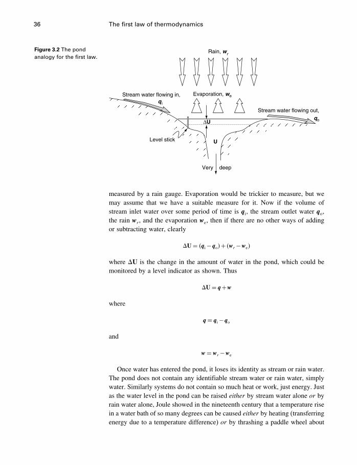
36 The first law of thermodynamics
Figure 3.2 The pondanalogy for the first law.
Rain, wr
Stream water flowing in, Evaporation, we
∆U
Stream water flowing out,
q i
qo
Level stick U
Very deep
measured by a rain gauge. Evaporation would be trickier to measure, but wemay assume that we have a suitable measure for it. Now if the volume ofstream inlet water over some period of time is qi, the stream outlet water qo,the rain wr , and the evaporation we, then if there are no other ways of addingor subtracting water, clearly
�U= �qi−qo�+ �wr −we�
where �U is the change in the amount of water in the pond, which could bemonitored by a level indicator as shown. Thus
�U= q+w
where
q= qi−qo
and
w= wr −we
Once water has entered the pond, it loses its identity as stream or rain water.The pond does not contain any identifiable stream water or rain water, simplywater. Similarly systems do not contain so much heat or work, just energy. Justas the water level in the pond can be raised either by stream water alone or byrain water alone, Joule showed in the nineteenth century that a temperature risein a water bath of so many degrees can be caused either by heating (transferringenergy due to a temperature difference) or by thrashing a paddle wheel about
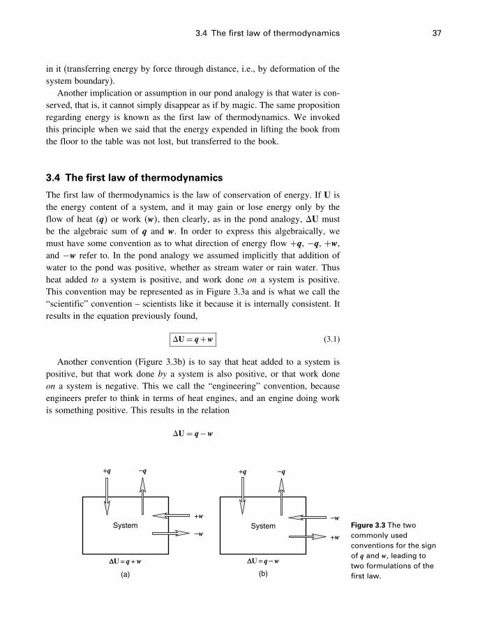
3.4 The first law of thermodynamics 37
in it (transferring energy by force through distance, i.e., by deformation of thesystem boundary).
Another implication or assumption in our pond analogy is that water is con-served, that is, it cannot simply disappear as if by magic. The same propositionregarding energy is known as the first law of thermodynamics. We invokedthis principle when we said that the energy expended in lifting the book fromthe floor to the table was not lost, but transferred to the book.
3.4 The first law of thermodynamics
The first law of thermodynamics is the law of conservation of energy. If U isthe energy content of a system, and it may gain or lose energy only by theflow of heat �q� or work �w�, then clearly, as in the pond analogy, �U mustbe the algebraic sum of q and w. In order to express this algebraically, wemust have some convention as to what direction of energy flow +q, −q, +w,and −w refer to. In the pond analogy we assumed implicitly that addition ofwater to the pond was positive, whether as stream water or rain water. Thusheat added to a system is positive, and work done on a system is positive.This convention may be represented as in Figure 3.3a and is what we call the“scientific” convention – scientists like it because it is internally consistent. Itresults in the equation previously found,
�U= q+w (3.1)
Another convention (Figure 3.3b) is to say that heat added to a system ispositive, but that work done by a system is also positive, or that work doneon a system is negative. This we call the “engineering” convention, becauseengineers prefer to think in terms of heat engines, and an engine doing workis something positive. This results in the relation
�U= q−w
(a)
System
+q –q
+w
–w
∆U = q + w
(b)
System
+q –q
–w
+w
∆U = q – w
Figure 3.3 The twocommonly usedconventions for the signof q and w, leading totwo formulations of thefirst law.
38 The first law of thermodynamics
and also results in slightly simpler equations expressing pressure–volume work(the minus signs in Equations (3.3) to (3.7) would be missing). In this text wewill use the scientific sign convention. Any additions of matter and energy tothe system are positive in sign and all losses are negative.
Note that we have not “proved” the first law. It is a principle that has beendeduced from the way things work in our experience, but the fact that it hasnever been known to fail does not constitute a proof. Neither does the fact thatthe sun has never failed to rise in the east constitute a proof that it will rise inthe east tomorrow, but I wouldn’t bet against it.
3.4.1 Work
Types of workThere are many different ways of doing work on a system, and many differentways of having a system do work, depending on what kinds of forces areavailable. For example,
• The force of gravity means that we have to do work to lift objects, as mentioned
above. If the mass is m, the acceleration due to gravity is g, and the distance is dh,
the work w is w=mg ·dh.3• Tensile force can be used to stretch a wire. If the tensile force is f and the increase
in length is dl, w= f ·dl.4• Tensile force can be used to increase the area of a soap film. If the surface tension is
and the increase in surface area is dA, then w= ·dA.• Expansion due to the heating of a gas, or indeed of anything at all, produces a
force. This case is of special interest to us, because the work done by expansion or
contraction of systems due to a change in temperature at constant pressure cannot be
avoided. We can choose to eliminate other forms of work, but not this one (unless
we consider only constant volume systems, which is useful at times, but not very
practical). It is treated in more detail below.• Chemical work. For example, a battery can be used to do work, because a chemical
reaction occurs in it which produces a voltage. The work done by chemical reactions
is of course a principal focus of chemical thermodynamics, and the equations for it
will be developed in later chapters.
There are others, such as work done by centripetal and frictional forces, thatyou can review in a physics text. Thermodynamics can accommodate all kindsof forces and types of work, but because they are in principle all the same, andare treated in the same way, it is simpler to develop the subject by considering
3 Don’t be confused by the differential term dh here. This is not (or at least not necessarily) aninfinitesimal distance. It is any distance in the h direction. We could call it �h, but we willlater include it in a differential equation (§4.7), so we might as well use the differentialnotation here too. It is only when we integrate that dh must become very, very small. This istreated in more detail in Appendix C.
4 This assumes the wire deforms elastically.
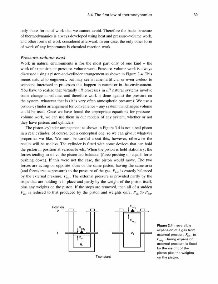
3.4 The first law of thermodynamics 39
only those forms of work that we cannot avoid. Therefore the basic structureof thermodynamics is always developed using heat and pressure–volume work,and other forms of work considered afterward. In our case, the only other formof work of any importance is chemical reaction work.
Pressure–volume workWork in natural environments is for the most part only of one kind – thework of expansion, or pressure–volume work. Pressure–volume work is alwaysdiscussed using a piston-and-cylinder arrangement as shown in Figure 3.4. Thisseems natural to engineers, but may seem rather artificial or even useless tosomeone interested in processes that happen in nature or in the environment.You have to realize that virtually all processes in all natural systems involvesome change in volume, and therefore work is done against the pressure onthe system, whatever that is (it is very often atmospheric pressure). We use apiston–cylinder arrangement for convenience – any system that changes volumecould be used. Once we have found the appropriate equations for pressure–volume work, we can use them in our models of any system, whether or notthey have pistons and cylinders.
The piston–cylinder arrangement as shown in Figure 3.4 is not a real pistonin a real cylinder, of course, but a conceptual one, so we can give it whateverproperties we like. We must be careful about this, however, otherwise theresults will be useless. The cylinder is fitted with some devices that can holdthe piston in position at various levels. When the piston is held stationary, theforces tending to move the piston are balanced (force pushing up equals forcepushing down). If this were not the case, the piston would move. The twoforces are acting on opposite sides of the same piston, having the same area(and force/area = pressure) so the pressure of the gas, Pint, is exactly balancedby the external pressure, Pext. The external pressure is provided partly by thestops that are holding it in place and partly by the weight of the piston itself,plus any weights on the piston. If the stops are removed, then all of a suddenPext is reduced to that produced by the piston and weights only, Pint � Pext,
Position2
1
Pext1
Pext2
Pint1
Pint2
V1
V2
T constant
Figure 3.4 Irreversibleexpansion of a gas fromexternal pressure Pext1
toPext2
. During expansion,external pressure is fixedby the weight of thepiston plus the weightson the piston.
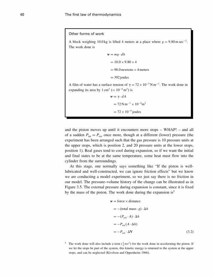
40 The first law of thermodynamics
Other forms of work
A block weighing 10.0 kg is lifted 4 meters at a place where g = 9�80m sec−2.
The work done is
w=mg ·dh= 10�0×9�80×4
= 98�0newtons×4meters
= 392 joules
A film of water has a surface tension of = 72×10−3 Nm−1. The work done in
expanding its area by 1 cm2 (= 10−4 m2) is
w= ·dA= 72Nm−1×10⁻⁴m2
= 72×10−4 joules
and the piston moves up until it encounters more stops – WHAP! – and allof a sudden Pint = Pext once more, though at a different (lower) pressure (theexperiment has been arranged such that the gas pressure is 10 pressure units atthe upper stops, which is position 2, and 20 pressure units at the lower stops,position 1). Real gases tend to cool during expansion, so if we want the initialand final states to be at the same temperature, some heat must flow into thecylinder from the surroundings.
At this stage, one normally says something like “If the piston is well-lubricated and well-constructed, we can ignore friction effects” but we knowwe are conducting a model experiment, so we just say there is no friction inour model. The pressure–volume history of the change can be illustrated as inFigure 3.5. The external pressure during expansion is constant, since it is fixedby the mass of the piston. The work done during the expansion is5
w= force×distance
=−�total mass ·g� ·�h=−�Pext ·A� ·�h=−Pext�A ·�h�=−Pext ·�V (3.2)
5 The work done will also include a term � 12mv2� for the work done in accelerating the piston. If
we let the stops be part of the system, this kinetic energy is returned to the system at the upperstops, and can be neglected (Kivelson and Oppenheim 1966).
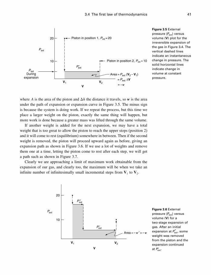
3.4 The first law of thermodynamics 41
Piston in position 1, Pint = 20
Piston in position 2, Pint = 10
Area = P
= Pext ∆V
= – wVV2V1
10
20
P ′
Pext
PextDuring
expansion
ext
ext (V2 – V1)
Figure 3.5 Externalpressure �Pext� versusvolume (V) plot for theirreversible expansion ofthe gas in Figure 3.4. Thevertical dashed linesindicate an instantaneouschange in pressure. Thesolid horizontal linesindicate change involume at constantpressure.
where A is the area of the piston and �h the distance it travels, so w is the areaunder the path of expansion or expansion curve in Figure 3.5. The minus signis because the system is doing work. If we repeat the process, but this time weplace a larger weight on the piston, exactly the same thing will happen, butmore work is done because a greater mass was lifted through the same volume.
If another weight is added for the next expansion, we may have a totalweight that is too great to allow the piston to reach the upper stops (position 2)and it will come to rest (equilibrium) somewhere in between. Then if the secondweight is removed, the piston will proceed upward again as before, giving anexpansion path as shown in Figure 3.6. If we use a lot of weights and removethem one at a time, letting the piston come to rest after each step, we will geta path such as shown in Figure 3.7.
Clearly we are approaching a limit of maximum work obtainable from theexpansion of our gas, and clearly too, the maximum will be when we take aninfinite number of infinitesimally small incremental steps from V1 to V2.
V
20
10
Area = – w ′ > – w
P ″
P ′
V1 V2
ext
ext
PextFigure 3.6 Externalpressure �Pext� versusvolume (V) for atwo-stage expansion ofgas. After an initialexpansion at P
′′ext, some
weight was removedfrom the piston and theexpansion continuedat P ′
ext.
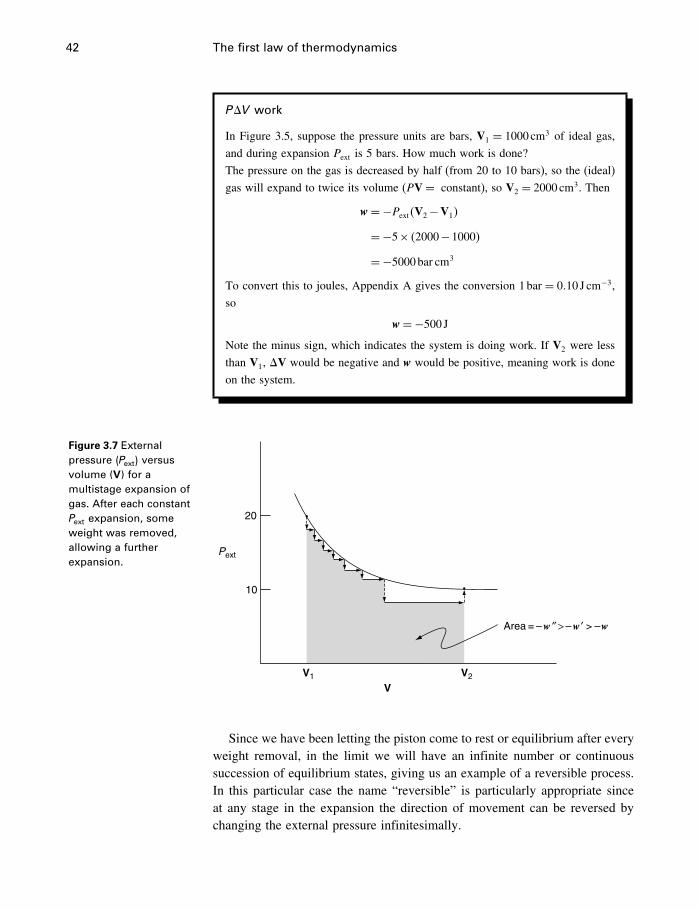
42 The first law of thermodynamics
P�V work
In Figure 3.5, suppose the pressure units are bars, V1 = 1000 cm3 of ideal gas,
and during expansion Pext is 5 bars. How much work is done?
The pressure on the gas is decreased by half (from 20 to 10 bars), so the (ideal)
gas will expand to twice its volume (PV= constant), so V2 = 2000 cm3. Then
w=−Pext�V2−V1�
=−5× �2000−1000�
=−5000bar cm3
To convert this to joules, Appendix A gives the conversion 1bar = 0�10 J cm−3,
so
w=−500 J
Note the minus sign, which indicates the system is doing work. If V2 were less
than V1, �V would be negative and w would be positive, meaning work is done
on the system.
Figure 3.7 Externalpressure �Pext� versusvolume (V) for amultistage expansion ofgas. After each constantPext expansion, someweight was removed,allowing a furtherexpansion.
Area = – w ″ > – w′ > – w
20
10
V1 V2
V
Pext
Since we have been letting the piston come to rest or equilibrium after everyweight removal, in the limit we will have an infinite number or continuoussuccession of equilibrium states, giving us an example of a reversible process.In this particular case the name “reversible” is particularly appropriate sinceat any stage in the expansion the direction of movement can be reversed bychanging the external pressure infinitesimally.
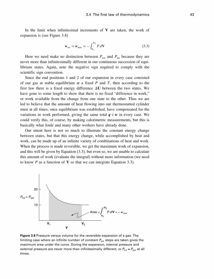
3.4 The first law of thermodynamics 43
In the limit when infinitesimal increments of V are taken, the work ofexpansion is (see Figure 3.8)
wrev = wmax =−∫ V2
V1
P dV (3.3)
Here we need make no distinction between Pext and Pint because they arenever more than infinitesimally different in our continuous succession of equi-librium states. Again, note the negative sign required to comply with thescientific sign convention.
Since the end positions 1 and 2 of our expansion in every case consistedof our gas at stable equilibrium at a fixed P and T , then according to thefirst law there is a fixed energy difference �U between the two states. Wehave gone to some length to show that there is no fixed “difference in work,”or work available from the change from one state to the other. Thus we areled to believe that the amount of heat flowing into our thermostatted cylindermust at all times, once equilibrium was established, have compensated for thevariations in work performed, giving the same total q+w in every case. Wecould verify this, of course, by making calorimetric measurements, but this isbasically what Joule and many other workers have already done.
Our intent here is not so much to illustrate the constant energy changebetween states, but that this energy change, while accomplished by heat andwork, can be made up of an infinite variety of combinations of heat and work.When the process is made reversible, we get the maximum work of expansion,and this will be given by Equation (3.3), but even so, we are unable to calculatethis amount of work (evaluate the integral) without more information (we needto know P as a function of V so that we can integrate Equation 3.3).
20
10
V1V
V2
Pint = Pext
V2
V1
Area = P d V = – wmax∫
Figure 3.8 Pressure versus volume for the reversible expansion of a gas. Thelimiting case where an infinite number of constant Pext steps are taken gives themaximum area under the curve. During the expansion, internal pressure andexternal pressure are never more than infinitesimally different, or Pint = Pext at alltimes.
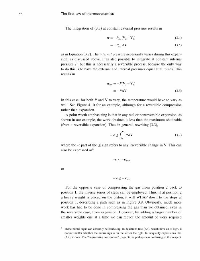
44 The first law of thermodynamics
The integration of (3.3) at constant external pressure results in
w=−Pext�V2−V1� (3.4)
=−Pext �V (3.5)
as in Equation (3.2). The internal pressure necessarily varies during this expan-sion, as discussed above. It is also possible to integrate at constant internalpressure P, but this is necessarily a reversible process, because the only wayto do this is to have the external and internal pressures equal at all times. Thisresults in
wrev =−P�V2−V1�
=−P�V (3.6)
In this case, for both P and V to vary, the temperature would have to vary aswell. See Figure 4.10 for an example, although for a reversible compressionrather than expansion.
A point worth emphasizing is that in any real or nonreversible expansion, asshown in our example, the work obtained is less than the maximum obtainable(from a reversible expansion). Thus in general, rewriting (3.3),
−w≤∫ V2
V1
P dV (3.7)
where the < part of the ≤ sign refers to any irreversible change in V. This canalso be expressed as6
−w≤−wmax
or
−w≤−wrev
For the opposite case of compressing the gas from position 2 back toposition 1, the inverse series of steps can be employed. Thus, if at position 2a heavy weight is placed on the piston, it will WHAP down to the stops atposition 1, describing a path such as in Figure 3.9. Obviously, much morework has had to be done in compressing the gas than we obtained, even inthe reversible case, from expansion. However, by adding a larger number ofsmaller weights one at a time we can reduce the amount of work required
6 These minus signs can certainly be confusing. In equations like (3.4), which have an = sign, itdoesn’t matter whether the minus sign is on the left or the right. In inequality expressions like(3.7), it does. The “engineering convention” (page 37) is perhaps less confusing in this respect.
3.4 The first law of thermodynamics 45
20
10
Position 1
Position 2
V2V1
V
Pext
Pext
Area = Work of compression≥ Work of expansion
Figure 3.9 Externalpressure �Pext� versusvolume for theirreversible compressionof gas at constant Pext.
for the compression, gradually approaching the stable equilibrium curve fromabove, rather than from below as before. In the limit, of course, we find thatfor a reversible compression the work required is exactly the same as the workavailable from a reversible expansion.
Considering this work stuff in such detail may make it look complex, but itreally is not. Just remember that if you need to calculate work (which happenssurprisingly little in geochemistry), you need either a constant pressure process,or a reversible one (so you can integrate). For “real” work processes, the workdone is invariably less than the reversible work (Equation 3.7), usually muchless, and usually of more interest to engineers than to geochemists.
3.4.2 Heat
It might be expected that since
�U= q+w
and
−w≤∫ V2
V1
P dV (3.8)
perhaps there is a very similar story for the heat transfers in the gas expansioncases we have been considering. That is, perhaps
−q≤∫ Z2
Z1
T dZ (3.9)
46 The first law of thermodynamics
where Z is some property of the gas. This is indeed the case (except for a signchange), but we must await the development of the second law, which willintroduce us to entropy (−Z in Equation 3.9).
3.4.3 The molar forms
Up to here we have considered total work, total heat and total energy involved inprocesses. In future chapters where we deal primarily with chemical reactions,it will often be more convenient to use the molar forms (§2.4.1), for example
�U = q+w (3.10)
w=−Pext�V (3.11)
wrev =−P�V (3.12)
−w≤∫ V2
V1
P dV (3.13)
and
−q≤∫ Z2
Z1
T dZ (3.14)
Forms of work other than the work done by chemical reactions are not usuallyexpressed in a molar form, so we could be more explicit by writing (3.12), forexample, as
wrev =−P�rV
but the less explicit form is not incorrect.
3.5 Enthalpy, the heat of reaction
In processes at constant external pressure, the work done, as we have seen(Equation 3.11), is−Pext�V .
7 In the present derivation it doesn’t matter whetherwe use Pext or P, as long as it is constant. Therefore the first law can be written
�U = qP−P �V
7 You might see Equation (3.11) written as w=−P �V . The difference is, to repeat, that Pext isthe (constant) external pressure (often it is atmospheric pressure) on the system which may beundergoing any sort of process, whereas unsubscripted P refers to the system pressure, whichcan have meaning only when the system is at equilibrium. Therefore if the system isundergoing a process, and P is constant, that process must be a reversible one, in which theheat flow in or out of the system constantly compensates for any tendency of the pressure tochange. See also Figure 4.10.
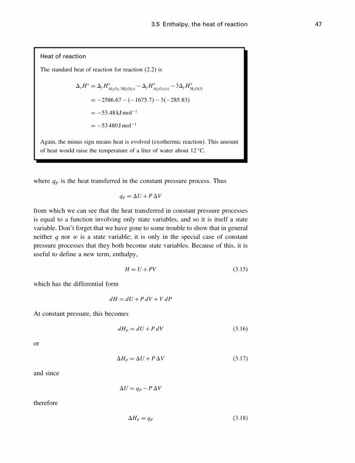
3.5 Enthalpy, the heat of reaction 47
Heat of reaction
The standard heat of reaction for reaction (2.2) is
�rH� = �fH
�Al2O3·3H2O�s�
−�fH�Al2O3�s�
−3�fH�H2O�l�
=−2586�67− �−1675�7�−3�−285�83�
=−53�48kJmol−1
=−53480 Jmol−1
Again, the minus sign means heat is evolved (exothermic reaction). This amount
of heat would raise the temperature of a liter of water about 12 �C.
where qP is the heat transferred in the constant pressure process. Thus
qP = �U +P �V
from which we can see that the heat transferred in constant pressure processesis equal to a function involving only state variables, and so it is itself a statevariable. Don’t forget that we have gone to some trouble to show that in generalneither q nor w is a state variable; it is only in the special case of constantpressure processes that they both become state variables. Because of this, it isuseful to define a new term, enthalpy,
H = U +PV (3.15)
which has the differential form
dH = dU +P dV +V dP
At constant pressure, this becomes
dHP = dU +P dV (3.16)
or
�HP = �U +P �V (3.17)
and since
�U = qP−P �V
therefore
�HP = qP (3.18)
48 The first law of thermodynamics
All we have done here is notice that, because work becomes a fixed quantityin constant pressure processes, then heat does too, by the first law. And becauseconstant pressure processes are so common (including all reactions carried outat atmospheric pressure, such as most biochemical reactions), it is convenientto have a state variable defined to equal this heat term. Defining enthalpy asin (3.15) accomplishes this, and we now have a “heat of reaction” term, whichwill be useful in all constant pressure processes.
Note that because H is a state variable, �H is perfectly well defined betweenany two equilibrium states. But when the two states are at the same pressure,�H becomes equal to the total heat flow during the process from one to theother, and in practice enthalpy is little used except in this context.8 Processeshaving a negative �rH (�rH < 0) are termed exothermic, and those having apositive �rH are termed endothermic.
3.5.1 Additivity of state variables
At several points in our discussions so far, we have mentioned or assumed thatwe can add and subtract state variables such as �H , for example as shownin Figure 5.3. This is perhaps obvious, but it is so fundamental that we willemphasize it here.
We said in Chapter 2 (§2.4) that a state variable is a property of a systemthat has a fixed value when the system is at equilibrium, whether we knowthe value of that property or not. For example, a mole of water at 25 �C,1 atm has a fixed but unknown enthalpy H , and fixed values of all other statevariables. We also said that this means that the changes in these propertiesbetween equilibrium states depends only on the equilibrium states, and not onwhat happens between the time the system leaves one equilibrium state andthe time it settles down in its new equilibrium state. Therefore, if two differentreactions produce the same compound, we can subtract the �rH
�, for example,of these reactions to get the � of the combined reaction, and the properties ofthat compound will cancel out. For example, carbon dioxide, CO2, might beproduced from the oxidation of either graphite or carbon monoxide, CO:
C+O2 = CO2 �rH� = −393�509kJmol−1
CO+ 12O2 = CO2 �rH
� = −282�984kJmol−1
Subtracting the reactions and the �rH� values (reverse the second reaction,
change the sign of �rH�, and add), we get
C+ 12O2 = CO �rH
� = −110�525kJmol−1
Thus we get the properties of a reaction that is impossible to carry out experi-mentally from two reactions that are relatively easy do experimentally.
8 Another use of the enthalpy is discussed in §6.2.3.
3.5 Enthalpy, the heat of reaction 49
3.5.2 Enthalpy of formation from the elements
A major problem arises from the definition of enthalpy, Equation (3.15). Theproblem is that we cannot measure it. This arises from the nature of energyitself, because we can only measure energy changes, not absolute energies.Therefore we can only measure enthalpy changes, and changes in any otherproperty which includes the energy U (or U ).
The problem this creates is that we do not want to have to tabulate anenthalpy change for every process or chemical reaction which might becomeof interest to us – there are too many. We would like to be able to associatean enthalpy with every substance – solids, liquids, gases, and solutes – forsome standard conditions, so that having tabulated these, we could then easilycalculate an enthalpy change between any such substances under those standardconditions. After that, we could deal with the changes introduced by impuritiesand other nonstandard conditions. The method developed to allow this is todetermine, for every pure compound, the difference between the enthalpy of thecompound and the sum of the enthalpies of the elements, each in its most stablestate, which make up the compound. This quantity is called �fH
�, the standardmolar enthalpy of formation from the elements. For aqueous ions, the quantitydetermined is a little more complicated (Chapter 15), but the principle is thesame. It is this enthalpy quantity which is invariably tabulated in compilationsof data.
For example, the standard enthalpy of formation of anhydrite is
�fH�CaSO4�s�
=H�CaSO4�s�
−H�Ca�s�−H�
S�s�−2H�O2�g�
(3.19)
where the superscript � refers to the standard conditions (see below). None ofthe individual H� quantities is determinable, but the difference is determinableby calorimetry. Now if we want to know the heat liberated or absorbed in achemical reaction, we need only look up these�fH
� values for each reactant andproduct. For example, for the formation of gypsum from anhydrite, we write
CaSO4�s�+2H2O�l�= CaSO4 ·2H2O�s� (3.20)
for which the “standard molar heat of reaction,” �rH�, is
�rH� = �fH
�CaSO4 ·2H2O
−�fH�CaSO4
−2�fH�H2O�l�
(3.21)
=H�CaSO4 ·2H2O
−H�CaSO4
−2H�H2O�l�
(3.22)
Note that in balanced reactions the H� terms for all the elements cancel out,and we are left with the “real” enthalpy difference (Equation 3.22) betweenproducts and reactants, with no contribution from arbitrary conventions orassumptions. It is, however, a heat of reaction for standard conditions only.
50 The first law of thermodynamics
Standard statesIt is often assumed that the “standard conditions” are 25 �C, 1 bar. Actually itis a bit more complicated in two respects.
1. Knowing the T and P of the state is not sufficient – we must also specify the physical
state of the substance. For solids and liquids, it is simply the pure substance (as in
our anhydrite-gypsum-water example) but for gases it is the gas acting ideally at one
bar (or 105 Pa), and for solutes it is the solute acting ideally at a concentration of
one molal. The reasons for these choices will be discussed later (Chapter 8).
2. While the temperature and pressure of the standard conditions are indeed 25 �C and
one bar for purposes of tabulating data, we can and often do have standard conditions
at any T and P.
These more complete definitions of our “standard conditions” define our stan-dard states, which will be seen to become particularly useful when we laterdefine the concept of activity (§8.2).
3.5.3 The heat capacity
An older name for the enthalpy is the “heat content.” This name is somewhatdiscredited for good reasons, but nevertheless it helps a little in conveyingthe essential idea behind the next concept, the heat capacity. The molar heatcapacity can be defined as the amount of heat required to raise the temperatureof one mole of a substance by one degree. Of course, some substances requiremuch more heat to do this than do others.
The formal definition is (dH
dT
)P
= CP (3.23)
or (d�H
dT
)P
= �CP (3.24)
or (d�H�
dT
)P
= �C�P (3.25)
Thus heat capacity is the rate of change in H or �H with T . A large CP meansthat H or �H changes a lot for a given change in T , i.e., it takes a lot of heatto raise the temperature.
It takes a different amount of heat to raise the temperature of a systemdepending on whether the volume or the pressure is kept constant, giving twodifferent quantities, CP and CV . CV is rarely used in geochemistry, but the heatcapacity at constant pressure, CP, is a surprisingly important quantity. It can
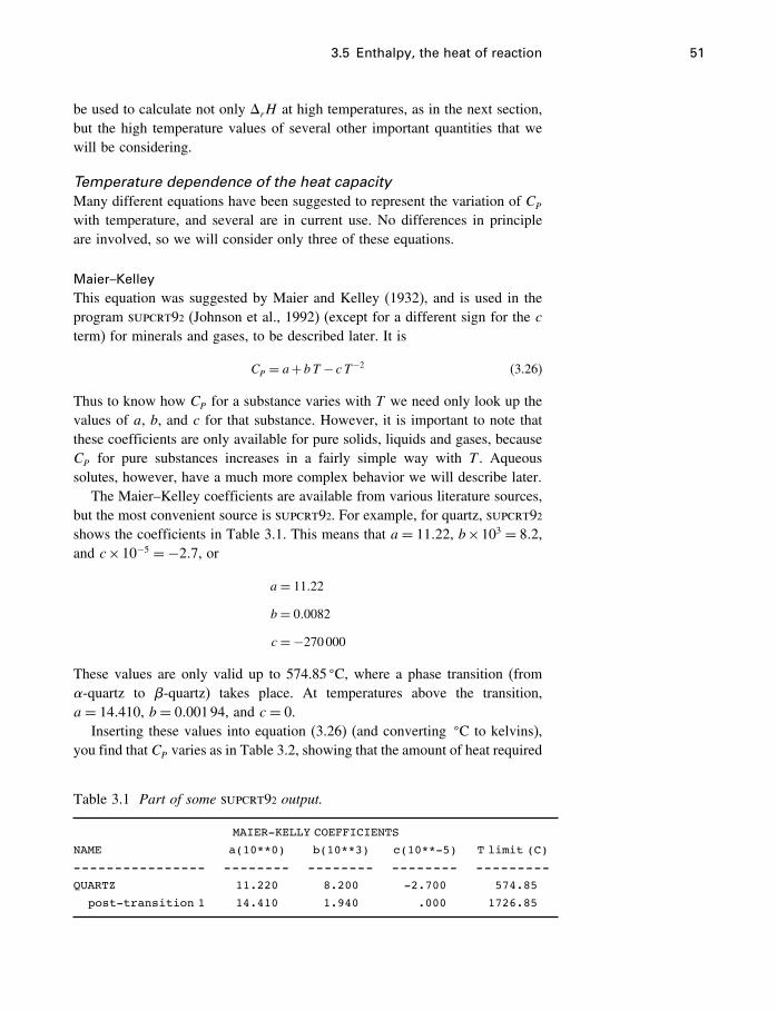
3.5 Enthalpy, the heat of reaction 51
be used to calculate not only �rH at high temperatures, as in the next section,but the high temperature values of several other important quantities that wewill be considering.
Temperature dependence of the heat capacityMany different equations have been suggested to represent the variation of CP
with temperature, and several are in current use. No differences in principleare involved, so we will consider only three of these equations.
Maier–KelleyThis equation was suggested by Maier and Kelley (1932), and is used in theprogram supcrt92 (Johnson et al., 1992) (except for a different sign for the cterm) for minerals and gases, to be described later. It is
CP = a+bT − c T−2 (3.26)
Thus to know how CP for a substance varies with T we need only look up thevalues of a, b, and c for that substance. However, it is important to note thatthese coefficients are only available for pure solids, liquids and gases, becauseCP for pure substances increases in a fairly simple way with T . Aqueoussolutes, however, have a much more complex behavior we will describe later.
The Maier–Kelley coefficients are available from various literature sources,but the most convenient source is supcrt92. For example, for quartz, supcrt92shows the coefficients in Table 3.1. This means that a= 11�22, b×103 = 8�2,and c×10−5 =−2�7, or
a= 11�22
b = 0�0082
c =−270000
These values are only valid up to 574.85 �C, where a phase transition (from-quartz to �-quartz) takes place. At temperatures above the transition,a= 14�410, b = 0�00194, and c = 0.
Inserting these values into equation (3.26) (and converting �C to kelvins),you find that CP varies as in Table 3.2, showing that the amount of heat required
Table 3.1 Part of some supcrt92 output.
MAIER-KELLY COEFFICIENTS
NAME a(10**0) b(10**3) c(10**-5) T limit (C)
---------------- -------- -------- -------- ---------
QUARTZ 11.220 8.200 -2.700 574.85
post-transition 1 14.410 1.940 .000 1726.85
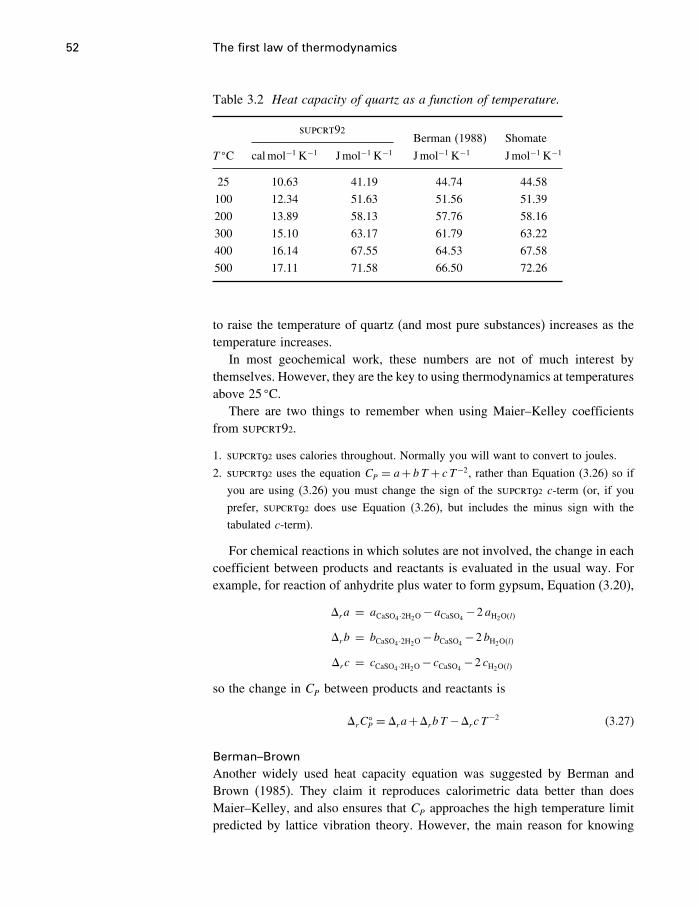
52 The first law of thermodynamics
Table 3.2 Heat capacity of quartz as a function of temperature.
supcrt92Berman (1988) Shomate
T �C calmol−1 K−1 Jmol−1 K−1 Jmol−1 K−1 Jmol−1 K−1
25 10.63 41.19 44.74 44.58
100 12.34 51.63 51.56 51.39
200 13.89 58.13 57.76 58.16
300 15.10 63.17 61.79 63.22
400 16.14 67.55 64.53 67.58
500 17.11 71.58 66.50 72.26
to raise the temperature of quartz (and most pure substances) increases as thetemperature increases.
In most geochemical work, these numbers are not of much interest bythemselves. However, they are the key to using thermodynamics at temperaturesabove 25 �C.
There are two things to remember when using Maier–Kelley coefficientsfrom supcrt92.
1. supcrt92 uses calories throughout. Normally you will want to convert to joules.
2. supcrt92 uses the equation CP = a+bT + c T−2, rather than Equation (3.26) so if
you are using (3.26) you must change the sign of the supcrt92 c-term (or, if you
prefer, supcrt92 does use Equation (3.26), but includes the minus sign with the
tabulated c-term).
For chemical reactions in which solutes are not involved, the change in eachcoefficient between products and reactants is evaluated in the usual way. Forexample, for reaction of anhydrite plus water to form gypsum, Equation (3.20),
�ra = aCaSO4 ·2H2O−aCaSO4
−2aH2O�l�
�rb = bCaSO4 ·2H2O−bCaSO4
−2bH2O�l�
�rc = cCaSO4 ·2H2O− cCaSO4
−2 cH2O�l�
so the change in CP between products and reactants is
�rC�P = �ra+�rbT −�rc T
−2 (3.27)
Berman–BrownAnother widely used heat capacity equation was suggested by Berman andBrown (1985). They claim it reproduces calorimetric data better than doesMaier–Kelley, and also ensures that CP approaches the high temperature limitpredicted by lattice vibration theory. However, the main reason for knowing
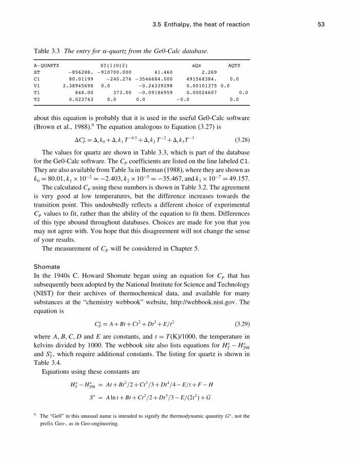
3.5 Enthalpy, the heat of reaction 53
Table 3.3 The entry for -quartz from the Ge0-Calc database.
A−QUARTZ SI(1)O(2) aQz AQTZST −856288. −910700.000 41.460 2.269C1 80.01199 −240.276 −3546684.000 491568384. 0.0V1 2.38945698 0.0 −0.24339298 0.00101375 0.0T1 848.00 373.00 −0.09186959 0.00024607 0.0T2 0.023743 0.0 0.0 −0.0 0.0
about this equation is probably that it is used in the useful Ge0-Calc software(Brown et al., 1988).9 The equation analogous to Equation (3.27) is
�C�P = �rk0+�rk1 T
−0�5+�rk2 T−2+�rk3T
−3 (3.28)
The values for quartz are shown in Table 3.3, which is part of the databasefor the Ge0-Calc software. The CP coefficients are listed on the line labeled C1.They are also available fromTable 3a in Berman (1988), where they are shown ask0 = 80�01, k1×10−2 =−2�403, k2×10−5 =−35�467, and k3×10−7 = 49�157.
The calculated CP using these numbers is shown in Table 3.2. The agreementis very good at low temperatures, but the difference increases towards thetransition point. This undoubtedly reflects a different choice of experimentalCP values to fit, rather than the ability of the equation to fit them. Differencesof this type abound throughout databases. Choices are made for you that youmay not agree with. You hope that this disagreement will not change the senseof your results.
The measurement of CP will be considered in Chapter 5.
ShomateIn the 1940s C. Howard Shomate began using an equation for CP that hassubsequently been adopted by the National Institute for Science and Technology(NIST) for their archives of thermochemical data, and available for manysubstances at the “chemistry webbook” website, http://webbook.nist.gov. Theequation is
C�P = A+Bt+Ct2+Dt3+E/t2 (3.29)
where A�B�C�D and E are constants, and t = T (K)/1000, the temperature inkelvins divided by 1000. The webbook site also lists equations for H�
T −H�298
and S�T , which require additional constants. The listing for quartz is shown inTable 3.4.
Equations using these constants are
H�T −H�
298 = At+Bt2/2+Ct3/3+Dt4/4−E/t+F −HS� = A ln t+Bt+Ct2/2+Dt3/3−E/�2t2�+G
9 The “Ge0” in this unusual name is intended to signify the thermodynamic quantity G�, not theprefix Geo-, as in Geo-engineering.
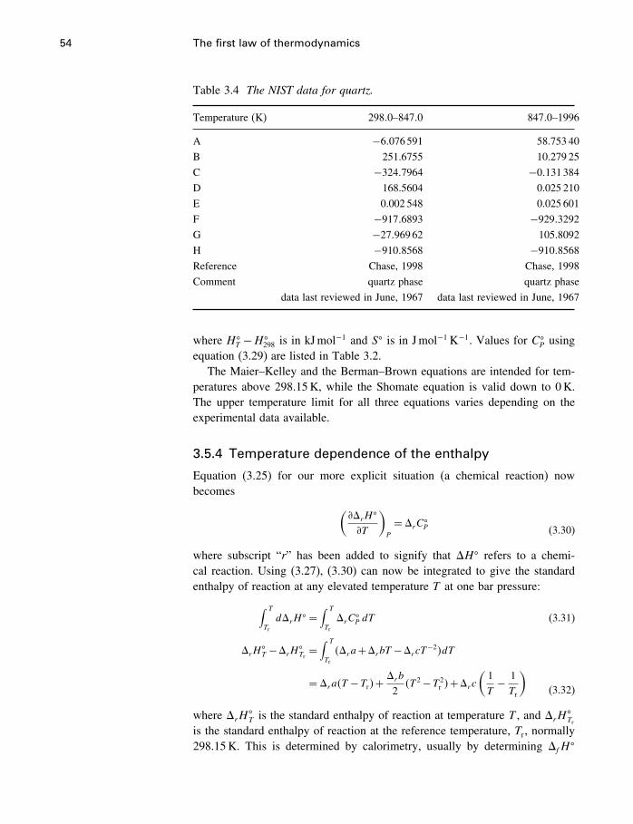
54 The first law of thermodynamics
Table 3.4 The NIST data for quartz.
Temperature (K) 298�0–847�0 847�0–1996
A −6�076591 58.753 40
B 251.6755 10.279 25
C −324�7964 −0�131384
D 168.5604 0.025 210
E 0.002 548 0.025 601
F −917�6893 −929�3292
G −27�96962 105.8092
H −910�8568 −910�8568
Reference Chase, 1998 Chase, 1998
Comment quartz phase quartz phase
data last reviewed in June, 1967 data last reviewed in June, 1967
where H�T −H�
298 is in kJmol−1 and S� is in Jmol−1 K−1. Values for C�P using
equation (3.29) are listed in Table 3.2.The Maier–Kelley and the Berman–Brown equations are intended for tem-
peratures above 298.15K, while the Shomate equation is valid down to 0K.The upper temperature limit for all three equations varies depending on theexperimental data available.
3.5.4 Temperature dependence of the enthalpy
Equation (3.25) for our more explicit situation (a chemical reaction) nowbecomes (
��rH�
�T
)P
= �rC�P (3.30)
where subscript “r” has been added to signify that �H� refers to a chemi-cal reaction. Using (3.27), (3.30) can now be integrated to give the standardenthalpy of reaction at any elevated temperature T at one bar pressure:∫ T
Tr
d�rH� =
∫ T
Tr
�rC�P dT (3.31)
�rH�T −�rH
�Tr=∫ T
Tr
��ra+�rbT −�rcT−2�dT
= �ra�T −Tr�+�rb
2�T 2−T 2
r �+�rc(1T− 1Tr
)(3.32)
where �rH�T is the standard enthalpy of reaction at temperature T , and �rH
�Tr
is the standard enthalpy of reaction at the reference temperature, Tr , normally298.15K. This is determined by calorimetry, usually by determining �fH
�
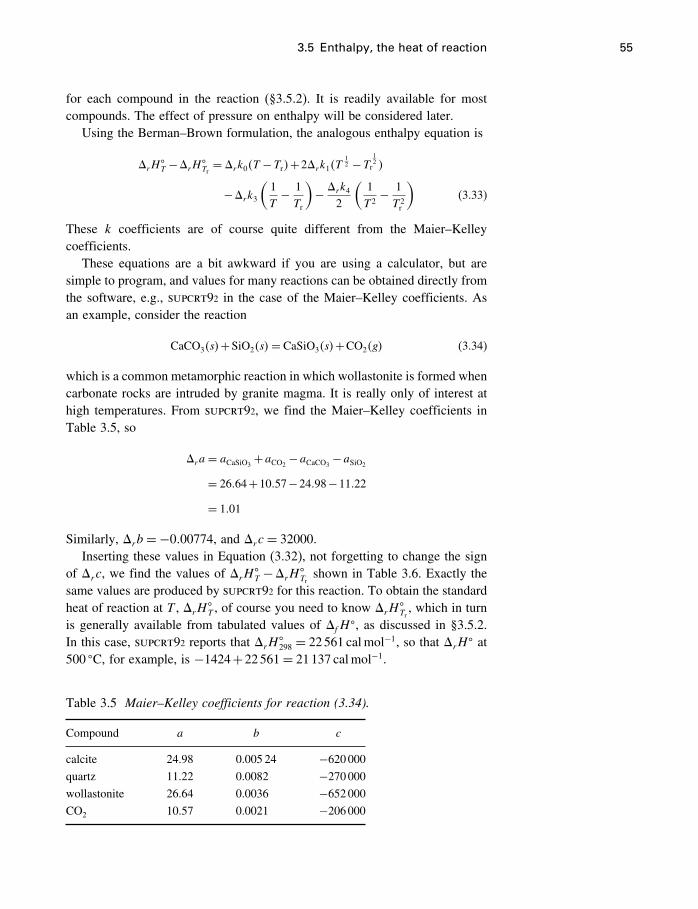
3.5 Enthalpy, the heat of reaction 55
for each compound in the reaction (§3.5.2). It is readily available for mostcompounds. The effect of pressure on enthalpy will be considered later.
Using the Berman–Brown formulation, the analogous enthalpy equation is
�rH�T −�rH
�Tr= �rk0�T −Tr�+2�rk1�T
12 −T 1
2r �
−�rk3(1T− 1Tr
)− �rk4
2
(1T 2
− 1T 2r
)(3.33)
These k coefficients are of course quite different from the Maier–Kelleycoefficients.
These equations are a bit awkward if you are using a calculator, but aresimple to program, and values for many reactions can be obtained directly fromthe software, e.g., supcrt92 in the case of the Maier–Kelley coefficients. Asan example, consider the reaction
CaCO3�s�+SiO2�s�= CaSiO3�s�+CO2�g� (3.34)
which is a common metamorphic reaction in which wollastonite is formed whencarbonate rocks are intruded by granite magma. It is really only of interest athigh temperatures. From supcrt92, we find the Maier–Kelley coefficients inTable 3.5, so
�ra= aCaSiO3+aCO2
−aCaCO3−aSiO2
= 26�64+10�57−24�98−11�22
= 1�01
Similarly, �rb =−0�00774, and �rc = 32000.Inserting these values in Equation (3.32), not forgetting to change the sign
of �rc, we find the values of �rH�T −�rH
�Trshown in Table 3.6. Exactly the
same values are produced by supcrt92 for this reaction. To obtain the standardheat of reaction at T , �rH
�T , of course you need to know �rH
�Tr, which in turn
is generally available from tabulated values of �fH�, as discussed in §3.5.2.
In this case, supcrt92 reports that �rH�298 = 22561 calmol−1, so that �rH
� at500 �C, for example, is −1424+22561= 21137 calmol−1.
Table 3.5 Maier–Kelley coefficients for reaction (3.34).
Compound a b c
calcite 24.98 0.005 24 −620000
quartz 11.22 0.0082 −270000
wollastonite 26.64 0.0036 −652000
CO2 10.57 0.0021 −206000
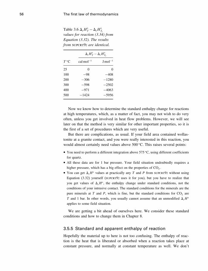
56 The first law of thermodynamics
Table 3.6 �rH�T −�rH
�Tr
values for reaction (3.34) fromEquation (3.32). The resultsfrom supcrt92 are identical.
�rH�T −�rH
�Tr
T �C calmol−1 Jmol−1
25 0 0
100 −98 −408
200 −306 −1280
300 −598 −2502
400 −971 −4063
500 −1424 −5956
Now we know how to determine the standard enthalpy change for reactionsat high temperatures, which, as a matter of fact, you may not wish to do veryoften, unless you get involved in heat flow problems. However, we will seelater on that the method is very similar for other important properties, so it isthe first of a set of procedures which are very useful.
But there are complications, as usual. If your field area contained wollas-tonite at a granite contact, and you were really interested in this reaction, youwould almost certainly need values above 500 �C. This raises several points:
• You need to perform a different integration above 575 �C, using different coefficients
for quartz.• All these data are for 1 bar pressure. Your field situation undoubtedly requires a
higher pressure, which has a big effect on the properties of CO2.• You can get �rH
� values at practically any T and P from supcrt92 without using
Equation (3.32) yourself (supcrt92 uses it for you), but you have to realize that
you get values of �rH�, the enthalpy change under standard conditions, not the
conditions of your intrusive contact. The standard conditions for the minerals are the
pure minerals at T and P, which is fine, but the standard conditions for CO2 are
T and 1 bar. In other words, you usually cannot assume that an unmodified �rH�
applies to some field situation.
We are getting a bit ahead of ourselves here. We consider these standardconditions and how to change them in Chapter 8.
3.5.5 Standard and apparent enthalpy of reaction
Hopefully the material up to here is not too confusing. The enthalpy of reac-tion is the heat that is liberated or absorbed when a reaction takes place atconstant pressure, and normally at constant temperature as well. We don’t
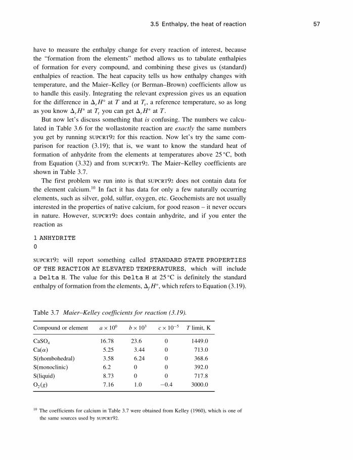
3.5 Enthalpy, the heat of reaction 57
have to measure the enthalpy change for every reaction of interest, becausethe “formation from the elements” method allows us to tabulate enthalpiesof formation for every compound, and combining these gives us (standard)enthalpies of reaction. The heat capacity tells us how enthalpy changes withtemperature, and the Maier–Kelley (or Berman–Brown) coefficients allow usto handle this easily. Integrating the relevant expression gives us an equationfor the difference in �rH
� at T and at Tr , a reference temperature, so as longas you know �rH
� at Tr you can get �rH� at T .
But now let’s discuss something that is confusing. The numbers we calcu-lated in Table 3.6 for the wollastonite reaction are exactly the same numbersyou get by running supcrt92 for this reaction. Now let’s try the same com-parison for reaction (3.19); that is, we want to know the standard heat offormation of anhydrite from the elements at temperatures above 25 �C, bothfrom Equation (3.32) and from supcrt92. The Maier–Kelley coefficients areshown in Table 3.7.
The first problem we run into is that supcrt92 does not contain data forthe element calcium.10 In fact it has data for only a few naturally occurringelements, such as silver, gold, sulfur, oxygen, etc. Geochemists are not usuallyinterested in the properties of native calcium, for good reason – it never occursin nature. However, supcrt92 does contain anhydrite, and if you enter thereaction as
1 ANHYDRITE0
supcrt92 will report something called STANDARD STATE PROPERTIESOF THE REACTION AT ELEVATED TEMPERATURES, which will includea Delta H. The value for this Delta H at 25 �C is definitely the standardenthalpy of formation from the elements, �fH
�, which refers to Equation (3.19).
Table 3.7 Maier–Kelley coefficients for reaction (3.19).
Compound or element a×100 b×103 c×10−5 T limit, K
CaSO4 16�78 23�6 0 1449�0
Ca() 5�25 3�44 0 713�0
S(rhombohedral) 3�58 6�24 0 368�6
S(monoclinic) 6�2 0 0 392�0
S(liquid) 8�73 0 0 717�8
O2�g� 7�16 1�0 −0�4 3000�0
10 The coefficients for calcium in Table 3.7 were obtained from Kelley (1960), which is one ofthe same sources used by supcrt92.
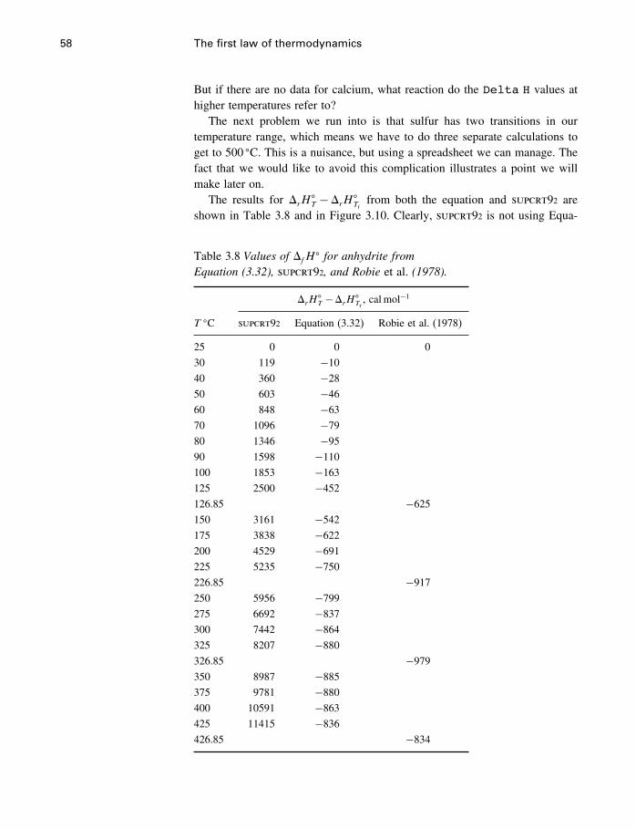
58 The first law of thermodynamics
But if there are no data for calcium, what reaction do the Delta H values athigher temperatures refer to?
The next problem we run into is that sulfur has two transitions in ourtemperature range, which means we have to do three separate calculations toget to 500 �C. This is a nuisance, but using a spreadsheet we can manage. Thefact that we would like to avoid this complication illustrates a point we willmake later on.
The results for �rH�T −�rH
�Tr
from both the equation and supcrt92 areshown in Table 3.8 and in Figure 3.10. Clearly, supcrt92 is not using Equa-
Table 3.8 Values of �fH� for anhydrite from
Equation (3.32), supcrt92, and Robie et al. (1978).
�rH�T −�rH
�Tr, cal mol−1
T �C supcrt92 Equation (3.32) Robie et al. (1978)
25 0 0 0
30 119 −10
40 360 −28
50 603 −46
60 848 −63
70 1096 −79
80 1346 −95
90 1598 −110
100 1853 −163
125 2500 −452
126.85 −625
150 3161 −542
175 3838 −622
200 4529 −691
225 5235 −750
226.85 −917
250 5956 −799
275 6692 −837
300 7442 −864
325 8207 −880
326.85 −979
350 8987 −885
375 9781 −880
400 10591 −863
425 11415 −836
426.85 −834
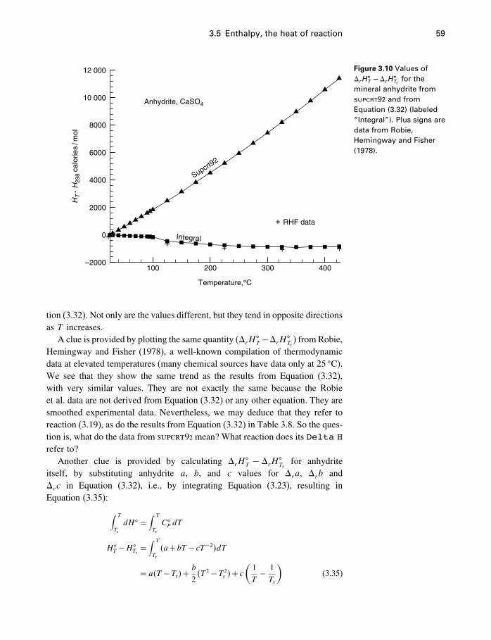
3.5 Enthalpy, the heat of reaction 59
Temperature,°C
HT
-H
298
calo
ries
/mol
100 200 300 400–2000
0
2000
4000
6000
8000
10 000
12 000
++ + + +
Supcrt92
Integral
+ RHF data
Anhydrite, CaSO4
Figure 3.10 Values of�rH
�T −�rH
�Tr
for themineral anhydrite fromsupcrt92 and fromEquation (3.32) (labeled“Integral”). Plus signs aredata from Robie,Hemingway and Fisher(1978).
tion (3.32). Not only are the values different, but they tend in opposite directionsas T increases.
A clue is provided by plotting the same quantity (�rH�T−�rH
�Tr) from Robie,
Hemingway and Fisher (1978), a well-known compilation of thermodynamicdata at elevated temperatures (many chemical sources have data only at 25 �C).We see that they show the same trend as the results from Equation (3.32),with very similar values. They are not exactly the same because the Robieet al. data are not derived from Equation (3.32) or any other equation. They aresmoothed experimental data. Nevertheless, we may deduce that they refer toreaction (3.19), as do the results from Equation (3.32) in Table 3.8. So the ques-tion is, what do the data from supcrt92 mean? What reaction does its Delta Hrefer to?
Another clue is provided by calculating �rH�T − �rH
�Tr
for anhydriteitself, by substituting anhydrite a, b, and c values for �ra, �rb and�rc in Equation (3.32), i.e., by integrating Equation (3.23), resulting inEquation (3.35): ∫ T
Tr
dH� =∫ T
Tr
C�P dT
H�T −H�
Tr=∫ T
Tr
�a+bT − cT−2�dT
= a�T −Tr�+b
2�T 2−T 2
r �+ c(1T− 1Tr
)(3.35)
60 The first law of thermodynamics
The results from this calculation are identical with the supcrt92 results,Figure 3.10.
What this means is that in the expression �H�T −�H�
Tr, the value of �H�
T
that supcrt92 calculates is not the difference in H� between anhydrite and∑H� of its constituent elements, all at T , but the difference between the H�
of anhydrite at T and∑H� of its constituent elements at Tr , 298.15K. This
called the apparent enthalpy of formation, �aH�.11 The value of �rH
�Tr, on the
other hand, is what it claims to be, the difference in H� of anhydrite and∑H�
of its constituent elements, all at Tr , which is in fact the heat of formation fromthe elements, �fH
�.
The Benson–Helgeson conventionThis way of doing things was started by Benson (1968) for enthalpy, and wasadopted by Helgeson in subsequent years for both enthalpy and other energyterms. Thus the Robie et al. (1978) enthalpy and free energy values include pro-vision for the change in the properties of the elements as temperature increases,while supcrt92, and any data in publications by Helgeson and the Berkeleygroup do not. There are distinct advantages in “neglecting” the elements atelevated temperatures, as in the Benson–Helgeson method. You can dispensewith finding coefficients for the elements for whatever heat capacity equationyou are using, and you don’t have to deal with all the phase transitions in theelements, such as those in sulfur that we complained about above. As long asyou deal only with balanced chemical reactions, the elements all cancel outanyway, so it does not matter what properties you assign to them. So if itdoesn’t matter, why not just leave them out?
Probably the vast majority of geochemists deal only with balanced reac-tions in considering geological problems, so they need never worry aboutwhether the “traditional,” Robie et al. method or the Benson–Helgeson methodis being used in their databases. But if you search the literature for data onspecific compounds, you must make sure you know how data above 25 �C arederived.
The Berman–Brown conventionBerman (1988), in presenting a widely used set of thermodynamic datafor metamorphic minerals, not only used a different heat capacity equation(Equation 3.28), but also a somewhat different method for “neglecting” theproperties of the elements. The Berman–Brown method is in fact the sameas Benson–Helgeson for enthalpy, but different for Gibbs energy (§5.7.1,page 144).
11 The use of apparent quantities is now so general that we will not usually bother with theseparate notation �aH or �aG. That is, we will use �fH and �fG, whatever convention isused.
3.7 The model again 61
3.6 How far have we got?
We have defined internal energy as some unspecified subset of the totalenergy in a system and considered the two common ways of changing thisenergy content. Along the way, we have noted that energy never disappears,and this is called the first law of thermodynamics. How far have we gottoward finding the “chemical energy,” that always decreases in spontaneouschanges?
Well, we’ve made the first vital step, but if you think about the previouschapters you’ll realize that we cannot have the answer yet. Why? Becausewe noted that some processes occur spontaneously with no energy change(ink spreading in water). Obviously, then, clarifying our thoughts about energychanges will not help in explaining processes that happen with no change inenergy of any kind.12 We still have some way to go toward defining a useful“chemical energy.”
3.7 The model again
In this chapter we have discussed some very practical operations. There is noth-ing particularly theoretical about gases expanding in cylinders and performingwork. It happens countless times every day all over the world. Equations suchas (3.2) belong to the real world. However, the result of the limit-taking, whenthe number of expansions or compressions in a single cycle is increased with-out limit, is a reversible process that belongs not to the real world but to thethermodynamic model. This is another illustration of the point made in §2.6.2,that energy differences between states can be calculated only for reversibleprocesses.
The equation
wrev =−∫ V2
V1
P dV [3.4]
is an extremely simple one, considered mathematically. If P can be expressedas an integrable function of V, then the integration is carried out and wrev isdetermined for a given change from V1 to V2. This presents absolutely noconceptual difficulties (beyond those in understanding calculus) if P and V aremathematical variables. However, if P and V represent measured pressures andvolumes from a real system in the real world, then even if P has been determinedas an integrable function of V for a number of individual measurements of P andV, the integration represents a variation of P with V that is impossible to carryout in the system. It is, however, simple to carry it out in the thermodynamic
12 Actually, we will note in the next chapter that the internal energy U is in fact the energy weneed to predict which way reactions will go under certain unusual conditions, but it is rarelyused in this sense.
62 The first law of thermodynamics
model, that is essentially mathematical and in that P as a function of V issimply a line in P–V space. This line represents a reversible process, a perfectlysimple and understandable facet of the thermodynamic model.
3.7.1 Applicability of the equations
Don’t forget – this conclusion about the work done due to a change in volumeis not only applicable to piston–cylinder arrangements. Virtually all chemicalreactions involve some change in volume between reactants and products, andthe equations are applicable no matter what the physical form of the reactantsand products. In other words, when corundum and water react to form gibbsite(Figure 2.2), the gibbsite occupies a different volume than does the sum ofthe volumes of the water and the corundum; therefore, some work is doneduring the reaction, and this work can be calculated using Equations (3.3) and(3.5). Even in reactions in living cells there will generally be a difference involume between products and reactants, and a constant pressure environment,and so some work is done during each and every biochemical reaction. Thiswork energy may be relatively small compared to the heat evolved or absorbedduring the same reactions, but it must always be considered. In reactions athigher pressures, it of course becomes even more important.
3.7.2 Clarifying notation
We have introduced quite a few subscripts and superscripts all at once here,which can be confusing. The logical relationships among these terms is shownin Figure 3.11, using H as an example. The same relationships will hold forother parameters we will introduce later.
The most general term for a change in H is simply �H . This refers toany change in the enthalpy of any system between two equilibrium states(stable or metastable), not necessarily associated with a chemical reaction.A special case is the �H between the products and reactants of a chemicalreaction, called �rH , so this represents a subset of the more general term �H .A special kind of chemical reaction involves only pure compounds, whosethermodynamic parameters can be found in tables, and so a subset of all �rH
values can be called �rH�, to indicate that all products and reactants are in
their pure reference states.13 A special case of �rH� is the reaction in which
a compound is formed from its elements, all in their pure reference states,and this is called �fH
�. Finally, we found that there are two conventions fordefining the enthalpy of formation from the elements, one being the traditionalor “common sense” method, where the compound and all its elements are at
13 Later on (Chapter 8) we will find that strictly speaking superscript � refers to a more general“standard state,” and that “pure reference states” are just one kind of standard state.
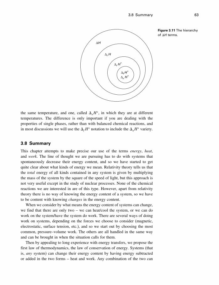
3.8 Summary 63
∆H
∆r H
∆r H
∆f H∆a H°
°
°
Figure 3.11 The hierarchyof �H terms.
the same temperature, and one, called �aH�, in which they are at different
temperatures. The difference is only important if you are dealing with theproperties of single phases, rather than with balanced chemical reactions, andin most discussions we will use the �fH
� notation to include the �aH� variety.
3.8 Summary
This chapter attempts to make precise our use of the terms energy, heat,and work. The line of thought we are pursuing has to do with systems thatspontaneously decrease their energy content, and so we have started to getquite clear about what kinds of energy we mean. Relativity theory tells us thatthe total energy of all kinds contained in any system is given by multiplyingthe mass of the system by the square of the speed of light, but this approach isnot very useful except in the study of nuclear processes. None of the chemicalreactions we are interested in are of this type. However, apart from relativitytheory there is no way of knowing the energy content of a system, so we haveto be content with knowing changes in the energy content.
When we consider by what means the energy content of systems can change,we find that there are only two – we can heat/cool the system, or we can dowork on the system/have the system do work. There are several ways of doingwork on systems, depending on the forces we choose to consider (magnetic,electrostatic, surface tension, etc.), and so we start out by choosing the mostcommon, pressure–volume work. The others are all handled in the same wayand can be brought in when the situation calls for them.
Then by appealing to long experience with energy transfers, we propose thefirst law of thermodynamics, the law of conservation of energy. Systems (thatis, any system) can change their energy content by having energy subtractedor added in the two forms – heat and work. Any combination of the two can
64 The first law of thermodynamics
result in the same total energy change; there is no specific “difference in heat”or “difference in work” between two different states of the same system.
Finally, we went into some detail on one special kind of energy transfer –the heat absorbed or released during a chemical reaction, where the initialand final states have the same pressure, generally referred to as a constantpressure reaction. This quantity of heat is the enthalpy, and it is one of thefundamental building blocks of our model. The fact that there are no absolutevalues for H is a decided nuisance, but a very simple way around this is byusing the “formation from the elements” convention. This means that for everycompound, we measure �H for the reaction in which a compound is formedfrom its elements, each in its most stable form, and these quantities are giventhe symbol �fH
�, where the subscript “f” stands for “formation from theelements,” and the superscript � means all substances are in their pure (exceptfor dissolved substances) reference states. The �H for any other reaction canthen be found by combining these �fH
� terms for compounds.Defining what we mean by energy and energy transfers is, of course, impor-
tant, but it does not by itself answer our questions about why reactions go oneway and not the other.
4The second law of thermodynamics
4.1 Introduction
The first sentence of Gibbs’ (1875) classic memoir “On the equilibrium ofheterogeneous substances” is
The comprehension of the laws which govern any material system is greatly
facilitated by considering the energy and entropy of the system in the various
states of which it is capable.
Given the fact that virtually all of equilibrium thermodynamics can be derivedby doing exactly that, as Gibbs did, this must rank as one of the world’s greatunderstatements. In this chapter, we begin to explore what Gibbs was referringto. By considering “the laws which govern any material system,” we shouldbe able to find the answers to the questions we posed in Chapter 1.
4.2 The problem restated
Having taken a couple of chapters to get our terminology settled and to getused to discussing energy changes in systems, we must now get back to ourmain problem – what determines whether chemical processes will go or not go?Our method of determining this might be considered a bit simple-minded – wewill simply determine the “chemical energy” differences between equilibriumstates. Processes can take place spontaneously if they are in the direction oflowering the chemical energy. They cannot take place spontaneously in theopposite direction.
We have seen that the first great principle of energy transfers is that energynever disappears; it simply takes on different forms. It is the second principle orlaw that more directly addresses our main problem. It is observed that once theconditions of the beginning and ending states are decided upon, processes canproceed spontaneously in only one direction between these states and are neverobserved to proceed in the other direction unless they are “pushed” with anexternal energy source. Thus for beginning and ending conditions of P = 1 barand T = 5 �C, ice will melt, but water will never spontaneously change to ice.
65
66 The second law of thermodynamics
We are looking for a “chemical energy” term that will always decrease in suchspontaneous reactions and will enable us to systematize and predict what wayreactions will proceed under given conditions. This may seem like a simpleproblem, but it is not.
The greatest single step forward in the development of thermodynamicswas the recognition and definition of a parameter, entropy, that enables suchpredictions and systematizations to be made. And yet, entropy still is not theenergy term we have been looking for; the energy that always decreases inspontaneous reactions. In fact, it is not even an energy term. Nevertheless, itis the secret to an understanding of spontaneous reactions.
4.2.1 What’s ahead
In this chapter, we will try to explain why this is so. As with the first law, thereis no way of proving the second law. It is a principle that is distilled from ourexperience of how things happen. It can be stated in a lot of different ways,usually having something to do with the impossibility of perpetual motion orwith the availability of energy, topics that seem to have little to do with theproblem we have set for ourselves – that of finding an energy term that alwaysdecreases in spontaneous reactions. We will choose to state it in a way thatemphasizes its role as a directionality parameter. This leads to the shortestpossible path to the practical applications we wish to consider.
So here’s the plan. We will define entropy as a parameter in our modelsystems, having certain properties. This definition is not, of course, pulled outof the blue, but is based on many years of work by many scientists. It shouldbe accepted at first on faith, as simply a useful parameter, because it will nothave any intuitive meaning as do our other terms such as energy, work, and soon. Then we will show how the “chemical energy” term we have been lookingfor is related to entropy. Finally, we will discuss what entropy is (and what itis not), and in Chapter 5, we will discuss how to measure it.
4.3 Thermodynamic potentials
At the start we should note that “directionality parameters” have a technicalname. They are called thermodynamic potentials. A potential in this sense is aquantity (a state variable) which is minimized (or maximized) at equilibrium,subject to certain constraints. This means that if you want to compare twostates of the same system to see which is the more stable, i.e., in which directionthe spontaneous change will “go,” two state variables must be the same in bothstates, and we call these two variables the constraints on the system. But notjust any two. Which two depends on which state variable you have chosen tobe maximized or minimized, i.e., on your choice of thermodynamic potential.Why two, and not one or three? Fundamentally it is because we chose to limit
4.4 Entropy 67
the ways our model systems can exchange energy to two: heat and only onekind of work, and we need one constraint for each of these.
For example, an appropriate thermodynamic potential would have a lowervalue for calcite than for aragonite at 25 �C, 1 bar (note that in saying 25 �C,1 bar we have chosen two constraints; one for heat and one for work). Generally,however, we have problems similar in principle but more complex. We mayhave several phases, including a solution with many compositional variables,and we will want to know the equilibrium compositions of all the phases at Tand P. In these cases there is a range of values for the thermodynamic potential,one for every possible composition of the phases involved, and we need tofind the minimum value of the potential. For any other value, greater thanthis minimum, some change in compositions (phases will dissolve, precipitate,etc.) will take place until the minimum value is achieved. We then speak ofminimizing the potential at a given T and P, i.e., subject to the given constraints.This is not a hypothetical problem, but a real problem in applied mathematics.We will see one way of doing this (speciation) in Chapter 16.
In this chapter we will identify four thermodynamic potentials. The numbercould in fact be extended – several other state variables with certain unusualconstraints can also be considered thermodynamic potentials. However, theyare never used in this sense, so we won’t bother with them. As a matterof fact, only one thermodynamic potential is ever used in geochemistry, butunderstanding is increased by learning about the others.
4.4 Entropy
4.4.1 Analogy
The first and most important thermodynamic potential we need is entropy.1 Oneway to define entropy would be to simply say that the Z-term in Equation (3.14)does indeed exist, where entropy is called S, and Z = −S. This provides auseful analogy between pressure–volume and temperature–entropy, and we willsee these terms linked together in many equations. They represent work andheat energy in many processes we will be considering.
This way of defining entropy is also useful in explaining a somewhat puz-zling feature of thermodynamics. In the next section, we will see that althoughentropy is a state variable of the kind we are looking for (one that can be used totell which way reactions will go), it is unfortunately one that increases in spon-taneous reactions, rather than decreasing, as we had supposed. This turns out
1 Strictly speaking, when identifying a thermodynamic potential, it is necessary to specify theconstraints. In other words, entropy (S) by itself is not a potential; entropy at constant energyand volume (SU�V) is a potential. In still other words, entropy is not maximized in systems atconstant T and P, only in systems at constant U and V.
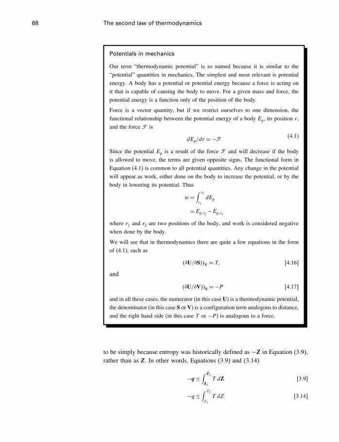
68 The second law of thermodynamics
Potentials in mechanics
Our term “thermodynamic potential” is so named because it is similar to the
“potential” quantities in mechanics. The simplest and most relevant is potential
energy. A body has a potential or potential energy because a force is acting on
it that is capable of causing the body to move. For a given mass and force, the
potential energy is a function only of the position of the body.
Force is a vector quantity, but if we restrict ourselves to one dimension, the
functional relationship between the potential energy of a body Ep, its position r ,
and the force � is
dEp/dr =−�(4.1)
Since the potential Ep is a result of the force � and will decrease if the body
is allowed to move, the terms are given opposite signs. The functional form in
Equation (4.1) is common to all potential quantities. Any change in the potential
will appear as work, either done on the body to increase the potential, or by the
body in lowering its potential. Thus
w =∫ r2
r1
dEp
= Ep�r2−Ep�r1
where r1 and r2 are two positions of the body, and work is considered negative
when done by the body.
We will see that in thermodynamics there are quite a few equations in the form
of (4.1), such as
��U/�S��V = T� [4.16]
and
��U/�V��S =−P [4.17]
and in all these cases, the numerator (in this case U) is a thermodynamic potential,
the denominator (in this case S orV) is a configuration term analogous to distance,
and the right hand side (in this case T or −P) is analogous to a force.
to be simply because entropy was historically defined as −Z in Equation (3.9),rather than as Z. In other words, Equations (3.9) and (3.14)
−q≤∫ Z2
Z1
T dZ [3.9]
−q≤∫ Z2
Z1
T dZ [3.14]
4.4 Entropy 69
are actually written
q≤∫ S2
S1T dS (4.2)
and
q≤∫ S2
S1
T dS (4.3)
that is, without the minus sign. This is a sort of “historical accident.” Because ofthe complete analogy between work–pressure–volume and heat–temperature–entropy (except for the minus sign), we can also write
qrev = T �S (4.4)
qrev = T �S (4.5)
analogous to (3.6) and (3.12),
wrev =−P�V [3.6]
wrev =−P�V [3.12]
A somewhat more mathematical way to express this analogy between work–pressure–volume and heat–temperature–entropy, and which is discussed inmore detail in §C.2.1, is to note that although wrev (or �wrev if you preferthat notation) is not the differential of any function (not an exact differential)wrev/P is, being equal to −�V , or −dV in differential notation. So one mightsuppose that similarly although qrev is not exact, perhaps qrev/T is. And indeedit is, being equal to dS.
4.4.2 Definition
However, a better way to define entropy is as follows. If there is indeed“something missing,” that is, only one thing missing from the energy-decreasing analogy, it is something that causes reactions to “go,” even whenno energy change whatsoever occurs. Now, we have defined a type of sys-tem (the isolated system) that does not permit energy changes to occur inthe system. Therefore, all we have to do is define a parameter with whichwe can predict reaction directions in this kind of system, combine it with theenergy-decreasing idea, and we should have our answer. This is what we dowith the following definition, paraphrased after Callen (1960). It can also serveas a statement of the second law of thermodynamics. The statement reflectsCallen’s “postulational” approach to thermodynamics, that is, let’s postulate
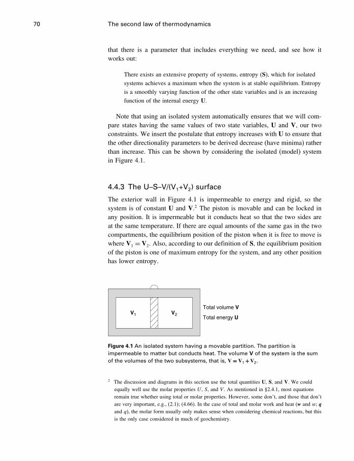
70 The second law of thermodynamics
that there is a parameter that includes everything we need, and see how itworks out:
There exists an extensive property of systems, entropy (S), which for isolated
systems achieves a maximum when the system is at stable equilibrium. Entropy
is a smoothly varying function of the other state variables and is an increasing
function of the internal energy U.
Note that using an isolated system automatically ensures that we will com-pare states having the same values of two state variables, U and V, our twoconstraints. We insert the postulate that entropy increases with U to ensure thatthe other directionality parameters to be derived decrease (have minima) ratherthan increase. This can be shown by considering the isolated (model) systemin Figure 4.1.
4.4.3 The U–S–V/(V1+V2) surface
The exterior wall in Figure 4.1 is impermeable to energy and rigid, so thesystem is of constant U and V.2 The piston is movable and can be locked inany position. It is impermeable but it conducts heat so that the two sides areat the same temperature. If there are equal amounts of the same gas in the twocompartments, the equilibrium position of the piston when it is free to move iswhere V1 = V2. Also, according to our definition of S, the equilibrium positionof the piston is one of maximum entropy for the system, and any other positionhas lower entropy.
V1 V2
Total volume V
Total energy U
Figure 4.1 An isolated system having a movable partition. The partition isimpermeable to matter but conducts heat. The volume V of the system is the sumof the volumes of the two subsystems, that is, V= V1 +V2.
2 The discussion and diagrams in this section use the total quantities U, S, and V. We couldequally well use the molar properties U , S, and V . As mentioned in §2.4.1, most equationsremain true whether using total or molar properties. However, some don’t, and those that don’tare very important, e.g., (2.1); (4.66). In the case of total and molar work and heat (w and w; qand q), the molar form usually only makes sense when considering chemical reactions, but thisis the only case considered in much of geochemistry.
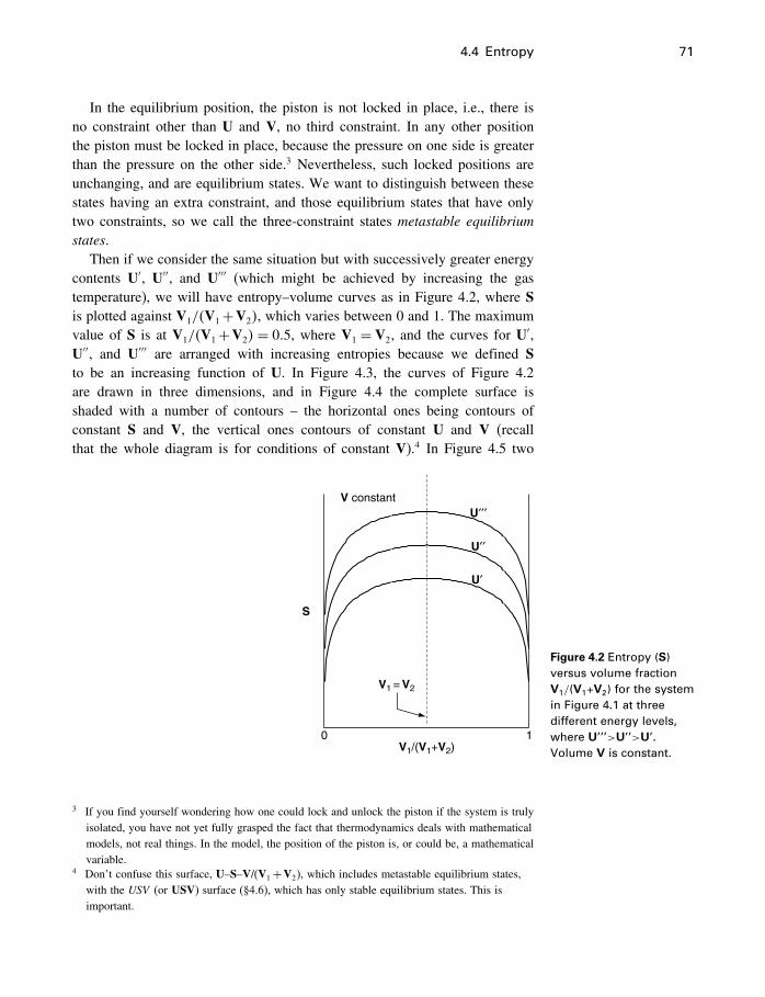
4.4 Entropy 71
In the equilibrium position, the piston is not locked in place, i.e., there isno constraint other than U and V, no third constraint. In any other positionthe piston must be locked in place, because the pressure on one side is greaterthan the pressure on the other side.3 Nevertheless, such locked positions areunchanging, and are equilibrium states. We want to distinguish between thesestates having an extra constraint, and those equilibrium states that have onlytwo constraints, so we call the three-constraint states metastable equilibriumstates.
Then if we consider the same situation but with successively greater energycontents U′, U′′, and U′′′ (which might be achieved by increasing the gastemperature), we will have entropy–volume curves as in Figure 4.2, where Sis plotted against V1/�V1+V2�, which varies between 0 and 1. The maximumvalue of S is at V1/�V1+V2� = 0�5, where V1 = V2, and the curves for U′,U′′, and U′′′ are arranged with increasing entropies because we defined Sto be an increasing function of U. In Figure 4.3, the curves of Figure 4.2are drawn in three dimensions, and in Figure 4.4 the complete surface isshaded with a number of contours – the horizontal ones being contours ofconstant S and V, the vertical ones contours of constant U and V (recallthat the whole diagram is for conditions of constant V).4 In Figure 4.5 two
0 1
S
V constantU′′′
U′′
U′
V1 = V2
V1/(V1+V2)
Figure 4.2 Entropy (S)versus volume fractionV1/(V1+V2) for the systemin Figure 4.1 at threedifferent energy levels,where U’’’>U’’>U’.Volume V is constant.
3 If you find yourself wondering how one could lock and unlock the piston if the system is trulyisolated, you have not yet fully grasped the fact that thermodynamics deals with mathematicalmodels, not real things. In the model, the position of the piston is, or could be, a mathematicalvariable.
4 Don’t confuse this surface, U–S–V/(V1+V2), which includes metastable equilibrium states,with the USV (or USV) surface (§4.6), which has only stable equilibrium states. This isimportant.
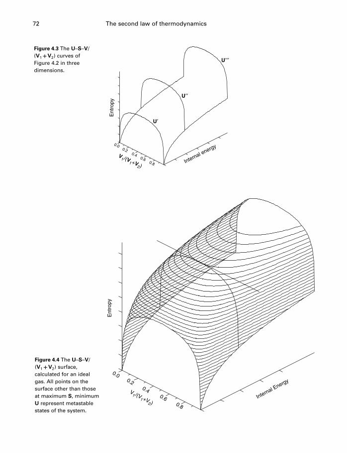
72 The second law of thermodynamics
Figure 4.3 The U–S–V/(V1 +V2) curves ofFigure 4.2 in threedimensions.
Internal energy
V1 /(V
1+V2 )
0.00.2
0.40.6
0.8
Ent
ropy
U′
U′′
U′′′
Internal Energy
0.8
0.6
0.4
0.2
0.0
Ent
ropy
V1 /(V
1+V2 )
Figure 4.4 The U–S–V/(V1 +V2) surface,calculated for an idealgas. All points on thesurface other than thoseat maximum S, minimumU represent metastablestates of the system.
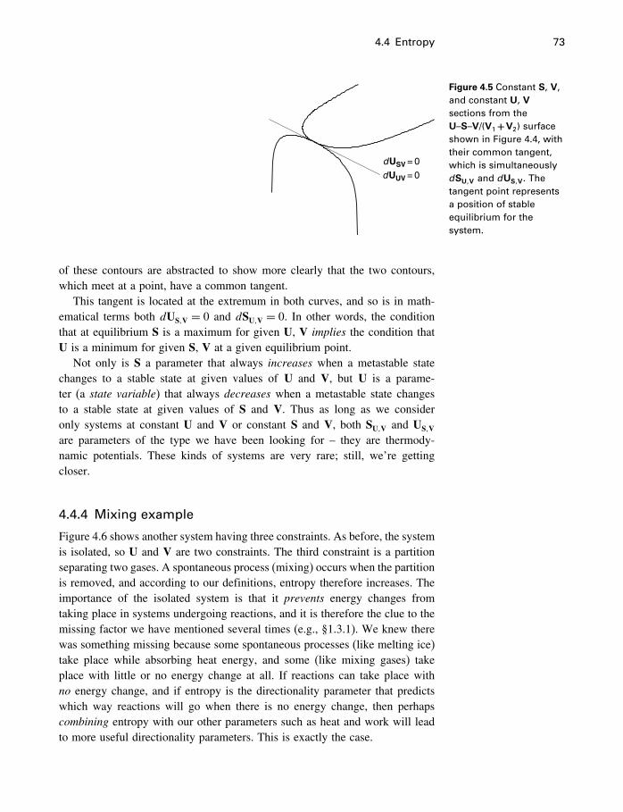
4.4 Entropy 73
dUSV = 0
dUUV = 0
Figure 4.5 Constant S, V,and constant U, Vsections from theU–S–V/(V1 +V2) surfaceshown in Figure 4.4, withtheir common tangent,which is simultaneouslydSU�V and dUS�V. Thetangent point representsa position of stableequilibrium for thesystem.
of these contours are abstracted to show more clearly that the two contours,which meet at a point, have a common tangent.
This tangent is located at the extremum in both curves, and so is in math-ematical terms both dUS�V = 0 and dSU�V = 0. In other words, the conditionthat at equilibrium S is a maximum for given U, V implies the condition thatU is a minimum for given S, V at a given equilibrium point.
Not only is S a parameter that always increases when a metastable statechanges to a stable state at given values of U and V, but U is a parame-ter (a state variable) that always decreases when a metastable state changesto a stable state at given values of S and V. Thus as long as we consideronly systems at constant U and V or constant S and V, both SU�V and US�V
are parameters of the type we have been looking for – they are thermody-namic potentials. These kinds of systems are very rare; still, we’re gettingcloser.
4.4.4 Mixing example
Figure 4.6 shows another system having three constraints. As before, the systemis isolated, so U and V are two constraints. The third constraint is a partitionseparating two gases. A spontaneous process (mixing) occurs when the partitionis removed, and according to our definitions, entropy therefore increases. Theimportance of the isolated system is that it prevents energy changes fromtaking place in systems undergoing reactions, and it is therefore the clue to themissing factor we have mentioned several times (e.g., §1.3.1). We knew therewas something missing because some spontaneous processes (like melting ice)take place while absorbing heat energy, and some (like mixing gases) takeplace with little or no energy change at all. If reactions can take place withno energy change, and if entropy is the directionality parameter that predictswhich way reactions will go when there is no energy change, then perhapscombining entropy with our other parameters such as heat and work will leadto more useful directionality parameters. This is exactly the case.
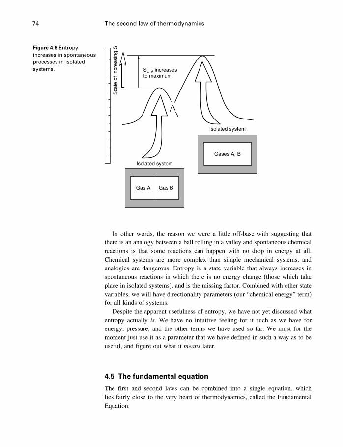
74 The second law of thermodynamics
Figure 4.6 Entropyincreases in spontaneousprocesses in isolatedsystems.
Isolated system
Isolated system
Gases A, B
Gas A Gas B
SU,V increasesto maximum
Sca
le o
f inc
reas
ing
S
In other words, the reason we were a little off-base with suggesting thatthere is an analogy between a ball rolling in a valley and spontaneous chemicalreactions is that some reactions can happen with no drop in energy at all.Chemical systems are more complex than simple mechanical systems, andanalogies are dangerous. Entropy is a state variable that always increases inspontaneous reactions in which there is no energy change (those which takeplace in isolated systems), and is the missing factor. Combined with other statevariables, we will have directionality parameters (our “chemical energy” term)for all kinds of systems.
Despite the apparent usefulness of entropy, we have not yet discussed whatentropy actually is. We have no intuitive feeling for it such as we have forenergy, pressure, and the other terms we have used so far. We must for themoment just use it as a parameter that we have defined in such a way as to beuseful, and figure out what it means later.
4.5 The fundamental equation
The first and second laws can be combined into a single equation, whichlies fairly close to the very heart of thermodynamics, called the FundamentalEquation.
4.6 The USV surface 75
Combining Equation (3.1) (�U = q+ w) with Equations (3.6) (wrev =−P �V) and (4.4) (qrev = T �S) (or Equations 3.12, 4.5 and 3.10) we obtain
�U= T �S−P �V (4.6)
and
�U = T �S−P �V (4.7)
These can also be written in differential notation as
dU= T dS−P dV (4.8)
and
dU = T dS−P dV (4.9)
This is probably the single most important equation in thermodynamics, andfor this reason it is called the Fundamental Equation.
It is worth mentioning that the “fundamental” nature of (4.9) does not meanthat we often use it directly. We usually use it after a little manipulation, sothat we can use integration limits of T and P, rather than S and V . In otherwords, we usually use Equation (4.37). Equation (4.9) is fundamental becauseit is directly linked to the first and second laws, and because Equation (4.37)and many others are derived from it.
4.6 The USV surface
4.6.1 Geometrical meaning of the fundamental equation
The easiest way to get a clear geometric picture of the fundamental equation isto realize that by virtue of the first law, every system at equilibrium, whetheras simple as an ideal gas or as complex as a bacterium, has a single fixedenergy content for given values of two independent variables, and by virtueof the second law we are able to use as variables S and V . Every systemcan therefore be represented by a surface in USV space, such as shown inFigure 4.7. Note that, in order to make the surface easier to draw, U increasesdownward in Figure 4.7. At every point on the surface, such as point A, therewill be a tangent surface, the equation for which is the fundamental equation,dU = T dS−P dV . Figure 4.8 shows how, starting at point A, increments ofdS and dV are combined with the slopes �U/�S and �U/�V to produce thetotal change in U at any other point on the tangent plane. In this case, eachof dU , dS, and dV has any magnitude, however large. Because of this, youmay visualize Equation (4.9) as having the form Z = aX+ bY , which is a
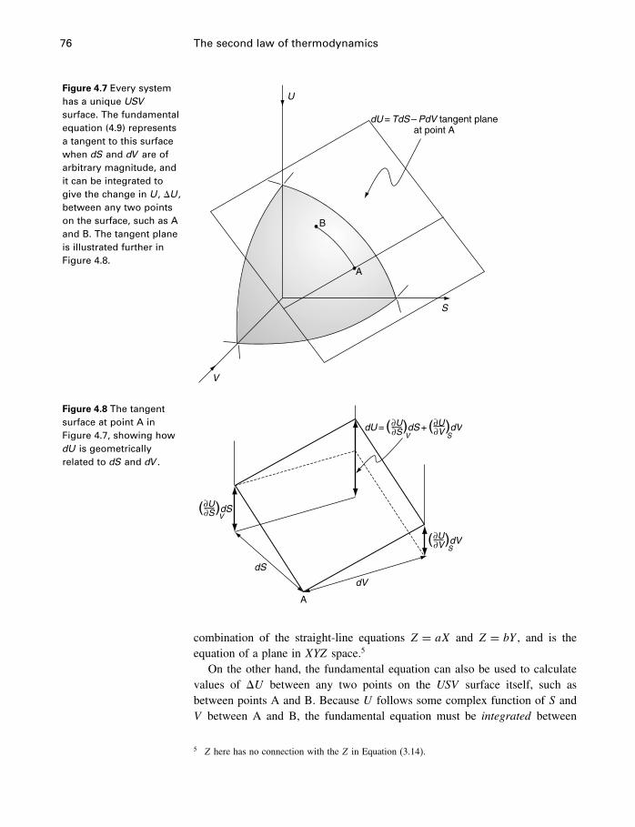
76 The second law of thermodynamics
Figure 4.7 Every systemhas a unique USV
surface. The fundamentalequation (4.9) representsa tangent to this surfacewhen dS and dV are ofarbitrary magnitude, andit can be integrated togive the change in U, �U,between any two pointson the surface, such as Aand B. The tangent planeis illustrated further inFigure 4.8.
S
V
U
B
A
dU = TdS – PdV tangent planeat point A
Figure 4.8 The tangentsurface at point A inFigure 4.7, showing howdU is geometricallyrelated to dS and dV .
dS
A
dV
dU = ( )dS + ( )dV
( )dS∂U∂S V
∂U∂S V
∂U∂V S
∂U∂V S
( )dV
combination of the straight-line equations Z = aX and Z = bY , and is theequation of a plane in XYZ space.5
On the other hand, the fundamental equation can also be used to calculatevalues of �U between any two points on the USV surface itself, such asbetween points A and B. Because U follows some complex function of S andV between A and B, the fundamental equation must be integrated between
5 Z here has no connection with the Z in Equation (3.14).
4.7 Those other forms of work 77
A and B, and this means allowing dS and dV to take on infinitesimal values6
and performing a summation, symbolized by the∫symbol. This is written
�U = UB−UA
=∫ B
AT dS−
∫ B
AP dV
The calculation of this difference follows the reversible path shown on theUSV surface – a continuous succession of equilibrium states, because that’swhat integration implies. However, the calculated �U is the same no matterhow the change from A to B is actually carried out.
The difference in U or in fact any thermodynamic property between a quartzcrystal at 25 �C and the same crystal at 50 �C has nothing to do with how thatdifference is achieved, but the calculation of that difference follows a reversiblepath. That just means we calculate the difference by integrating an equation.If you have difficulty understanding differential equations as used here, studyFigures 4.7 and 4.8.
4.7 Those other forms of work
Even though we hardly ever need to include other kinds of work in ourfundamental equation, it will prove useful to have a brief look at what thisequation looks like when they are included. Because many work terms don’tmake much sense in the molar form, we use the total energy form of thefundamental Equation (4.8). A very general formulation, including all forms ofwork, is
dU= T dS︸︷︷︸heat
− ∑i Xi dxi︸ ︷︷ ︸
all forms of work
(4.10)
where X is a generalized force and dxi a generalized displacement. Normally,we consider Xi to be −P and xi to be V or V , and we get the fundamentalequation. We considered a few other possibilities for the
∑i Xi dxi term in
§3.4.1. So, for example, if a system could exchange energy because of gravityacting on a mass m in addition to P–V work, Equation (4.9) would become
dU= T dS︸︷︷︸heat
−P dV+mgdh︸ ︷︷ ︸work
(4.11)
For the tensile force and surface tension forms of work we would have
dU= T dS︸︷︷︸heat
−P dV+f dl︸ ︷︷ ︸work
(4.12)
6 See Appendix C, page 589. for a note on infinitesimals and integration.
78 The second law of thermodynamics
and
dU= T dS︸︷︷︸heat
−P dV+ dA︸ ︷︷ ︸work
(4.13)
The chemical work term that we mentioned in §3.4.1 is −�d�, where � isthe affinity and � is the progress variable, resulting in
dU= T dS︸︷︷︸heat
− P dV︸ ︷︷ ︸PV work
− �d�︸ ︷︷ ︸chemical work︸ ︷︷ ︸
work
(4.14)
and, of course we could have any or all combinations, at least in principle.These equations should be fairly intuitive – dU represents the change in totalenergy of a system, and the three terms on the right are the three sources ofenergy change – heat, P–V work, and another kind of work. Because we areso interested in chemical reactions, we have a great deal more to say aboutEquation (4.14).
4.8 Applicability of the fundamental equation
For such a simple relationship, Equation (4.9) traditionally generates quite a bitof confusion. This is of two types, or perhaps two aspects of the same problem.That problem is reversibility versus irreversibility.
Equations (4.7) and (4.9)
�U = T �S−P �V [4.7]
dU = T dS−P dV [4.9]
appear to be limited to reversible processes, as both (3.12) and (4.5)
wrev =−P�V [3.12]
qrev = T �S [4.5]
refer to reversible processes. But this is not the case, which can be explainedin various ways.
1. For one thing, Equations (4.7) and (4.9) contain only state variables (U , S, and V , in
addition to T and P). Therefore, because the changes in state variables do not depend
on the nature of the change, Equation (4.7) (or the integration of Equation 4.9) is true
for any change between two equilibrium states which have the same composition,
with one important exception (see §4.8.1).
2. Although Equations (3.13) and (3.14) will both be untrue in an irreversible process,
the amount by which they become untrue (resulting in −w < P�V and q < T�S)
will cancel when they are added together. We could give examples of this, but it
must be true because of item 1.
4.9 Constraints and metastable states 79
3. In Figure 4.7, points A and B represent two stable equilibrium states of a system.
Integration of the fundamental equation from A→B takes place on the USV surface,
as shown, which is necessarily a reversible process. An irreversible process A→B
would cause the system to leave the surface at A, be not representable in USV space
between A and B, then the system would reappear at B. In either case, �U , �S, and
�V are related by Equation (4.7).
4.8.1 Two kinds of irreversibility
So the Equation (4.9) applies to reversible and irreversible processes. Thereremains the “important exception” just mentioned. The problem here is thatthere are two very different kinds of irreversible processes.7
1. One kind of irreversibility involves a system changing from one equilibrium state
to another. The equilibrium state can be stable or metastable (in the thermodynamic
sense, discussed below), as long as there is no change from one to the other (i.e.,
metastable→stable). For example Equation (4.9) can be applied to increments of
changes such as the irreversible gas expansion in Figure 3.4, or perhaps the irre-
versible heating of a crystal from 25 to 50 �C by simply putting it in an oven at
50 �C. The crystal could be (stable) calcite or (metastable) aragonite. Integrating
Equation (4.9) applies to all these processes. They could be thought of as processes
in response to a change in the first and/or second constraints.
2. But Equation (4.9) does not apply to irreversible processes in which a metastable
state changes to a stable state, such as a crystal of aragonite at some T and P within
the calcite stability field recrystallizing to calcite. Equations (4.14) and (4.46) apply
to these cases. In these cases a second form of work (non-PV work) is being done.
In one sense, it is perfectly obvious that if there is more than one formof work involved, you need one of the equations in §4.7, not Equation (4.9).In geochemistry, and most of chemistry, the only other form of work of interestis chemical work, and so the equation we use to represent a chemical reactionprogressing towards stable equilibrium is (4.14), or more usually (lookingahead) (4.46).
The most general way of expressing the applicability of the fundamentalequation is that it applies to any process which does not involve release of athird constraint.
4.9 Constraints and metastable states
We introduced the idea of constraints and metastable states in §4.4.3. Becauseof the importance of these concepts, we take a closer look at them here.
7 We mentioned these briefly in §2.6, page 21.
80 The second law of thermodynamics
4.9.1 Metastable states
It is here that distinguishing between real systems and our model systemsbecomes most valuable.
Real metastable statesThe distinction between stable and metastable equilibrium according to mostsources is that the stable equilibrium state is “truly unchanging,” or unchanginggiven indefinite time, whereas the metastable state may be changing, but tooslowly to be observed. This distinction clearly refers to real systems, and isoften very difficult to make. We know that at 25 �C, 1 bar, calcite is the moststable form of CaCO3. Aragonite is another form, and although it does notchange to calcite on museum shelves, it does change in nature under someconditions, given very long time periods, so is it metastable or unstable? Isvolcanic glass an unstable or a metastable phase? These questions can startarguments among geochemists. There are many reactions for which kinetic rateconstants are known at high temperatures (the reacting assemblage is thereforeunstable), but not at 25 �C, where the assemblage is considered metastable. Atwhat temperature does metastable change to unstable? If anyone was interested,the answer would of course be completely arbitrary. The kinetics of very slowlychanging systems is a problem for real systems, but it is not a problem inthermodynamics.
Thermodynamic metastable statesIn thermodynamics, a metastable equilibrium state has at least three constraints.Two of these constraints apply to a stable equilibrium state, and the third pre-vents the system from achieving that state.8 On releasing the third constraintthe system experiences a spontaneous process and achieves the stable equilib-rium state. We have seen two examples so far, in Figures 4.1 and 4.6. Theseexamples were chosen to follow from our definition of entropy, and showspontaneous processes having no overall energy change in the system. Theyshow entropy acting as a thermodynamic potential.
However, processes happening in isolated systems are pretty rare, in factstrictly speaking they are nonexistent. We need to develop other, moreuseful thermodynamic potentials (§4.12), to deal with the usual type ofmetastable→stable processes such as aragonite→calcite which invariablyinvolve a decrease in system energy. But even without doing that, we cansee several other examples of thermodynamic metastable states by looking
8 Actually, to be quite accurate, we should put the previous sentence in mathematical terms. Itwould then read Two of these constraints represent the independent variables of a functionsimulating the energy content of a physical system, and the third represents a possibleadditional independent variable. However, that has the disadvantage of obscuring the physicalmeaning of the constraints.

4.9 Constraints and metastable states 81
at the equations in §4.7. In each equation we see the fundamental equation,dU= T dS−P dV. Taking only one example, Equation (4.12), applying forcef to stretch a wire obviously does work on the wire (adds energy to the sys-tem), and releasing the force allows the wire to do work and resume its stableequilibrium state. While stretched, the system is in a metastable state. Similarstatements apply to the other equations. In each case, doing work on the systemputs it in a higher energy state (U is increased) and is held there by the thirdconstraint. Releasing the constraint allows the system to do work in a sponta-neous process. We give a more precise definition of constraints in §4.9.2. Theserelationships are illustrated in Figure 4.9a for the system Al2O3–H2O, wherethe arrow A→ A′ refers to a “chemical work” term, as in Equation (4.14).
S
Corundum + water surface
Corundum + water surface
U
V
T
P
G
(a)
(b)
A
A′
Gibbsite surface
Gibbsite surface
A
A′
Figure 4.9(a) Two equilibrium statesof the system Al2O3–H2Oin USV space: metastablecorundum plus water,and stable gibbsite. Theprocess A→A′ isreaction (2.2). Changes inU along either surfacecan be described byEquation (4.9). Changesin U between the surfaces(A→A′) are described byEquation (4.14). (b) Thesame system in GTP
space. Note that U and Gincrease downwards.
82 The second law of thermodynamics
Real systems may be truly unchanging and metastable, or they may beunstable and changing very, very slowly. Often we don’t know which. But ourmodels of systems have no such uncertainty. Metastable systems are modeledas in complete thermodynamic equilibrium, with (at least) three constraints. Ifthe real system is really unstable, our model is in this respect incorrect, butgenerally useful nonetheless.
4.9.2 Constraints
Constraint, like several other terms, has a slightly different meaning in real andmodel systems. Real systems, such as aragonite, are said to be constrained fromreacting to a more stable state (calcite) by an activation energy barrier. Theusage is rather imprecise, because we don’t actually know if the aragonite ischanging on some very long time scale or not. In model systems, the meaningis much more exact. A constraint in mathematics is a condition that must beobserved. For example you might want to find the minimum value of a functionof many variables, while assigning constant values to some of the variables.Each variable held constant is a constraint on the solution. In thermodynamicsit is essentially the same thing. We minimize some function of many variableswhile constraining two state variables to constant (known) values. We constraintwo, because in the first law we define only two ways of changing the energyof a system, heat and P–V work. If there is a third way of changing energy, athird state variable must be constrained – a third constraint. The system must bein some equilibrium state for that variable, or any variable, to be defined. Theonly thermodynamic equilibrium state that is not a stable equilibrium state is ametastable equilibrium state. A thermodynamic constraint, then, is defined as astate variable, associated with some method of changing system energy, that isheld constant while minimizing a thermodynamic potential. Stable equilibrium
Constraints in mechanics
Constraints, along with potentials, work, and energy, is another topic common to
thermodynamics and mechanics. The motion of bodies in mechanics is subject not
only to the force applied, but also to whatever constraints are present. A marble
rolling on the surface of a bowl is constrained to remain on the surface. Beads
on a string are constrained to move in a straight line, and so on.
Constraints in mechanics can be classified into various types, for example as
to whether the equation of constraint contains time as a variable or not. In
thermodynamics, which has only scalar variables, and which has no time variable,
constraints are simpler, and are identified with ways in which systems can change
their energy content.
4.10 The energy inequality expression 83
requires two constraints. Any extra constraints result in equilibrium states withgreater energy contents we call metastable.9
4.10 The energy inequality expression
Stable equilibrium states are the target destination for all metastable states,once their constraints are released. What equations refer to this process? Wetry here to make these important relationships fairly intuitive.
Equation (4.8) can also be written in the form of a total differential as
dU=(�U�S
)V
dS+(�U�V
)S
dV (4.15)
showing that, comparing with (4.8),(�U�S
)V
= T (4.16)
and (�U�V
)S
=−P (4.17)
which are the slopes of the USV surface in the V and S directions.The USV surface defined by this equation has an energy U defined for
given values of the two constraint variables S and V. It refers to changes inenergy between stable equilibrium states of a system (which may take placereversibly or irreversibly). At given values of S and V, a metastable state willhave greater values of U than those represented by this surface, and it will beheld in that state by a third constraint of some kind. Examples of equationshaving a third constraint are shown in §4.7.
Consider the wire-stretching example (Equation 4.12) again. If we imposea third constraint, i.e., we do non-PV work on the system like stretching thewire, we increase the value of U (dl and therefore f dl is positive).10 When theconstraint is released, the wire shrinks back to its former length, and the systemlowers its U irreversibly to the stable value.11 During this process, the shrinking
9 Clearly, isolated systems are an exception to this last statement (i.e., the statement thatapplying a third constraint results in a state with greater energy). We applied a constraint in anisolated system in two cases, illustrated in Figures 4.1 and 4.6, resulting in metastable states,but with no increase in system energy. In all simulations of real processes, however, thestatement is true.
10 At this point you may well wonder why the PV work term has a negative sign, while all theother work terms are positive. In PV work adding energy decreases the volume, so dV isnegative, but in all the other cases, increasing energy increases the displacement or differentialterm. For example in stretching a wire, dl is positive. Therefore only for PV work do we usethe negative sign to make P dV positive for a positive energy change.
11 You might also be wondering, what if I release the constraint reversibly? Can’t be done.That’s like supposing a ball can roll downhill reversibly.
84 The second law of thermodynamics
wire can do useful work. Therefore for any irreversible process (meaning anyprocess in which the third constraint is released12) U decreases, the third termon the right side becomes negative (e.g., dl is negative), and if we don’t includethis negative term, we can only write
dU< T dS−P dV (4.18)
Combining (4.18) and (4.9), a general fundamental equation for all states ofthe system is
dU≤ T dS−P dV (4.19)
If S and V are constant, dS= 0 and dV= 0, and it follows from (4.19) that
dUS�V ≤ 0 (4.20)
which is analogous to (4.28), and shows that the second law provides anothercriterion for spontaneous processes, this time that U is minimized at equilibriumin systems having constant values of S and V. It is another thermodynamicpotential. We saw this previously in graphical form in Figure 4.5.
Let’s just look at Equation (4.20) a little more closely. Breaking it intoseparate statements, it says
dUS�V < 0 for irreversible processes, (4.21)
dUS�V = 0 at equilibrium (4.22)
These equations actually imply the existence of a third constraint. They implythe existence of a function U with independent variables S and V and a thirdindependent variable, because if S and V are constant, the system cannot changeits energy by heat or PV work. U can only change using a second work terminvolving increments of a third constraint, and that change is always negativefor irreversible processes (Equation 4.21). Equation (4.22) says that U is at aminimum (or maximum) of some continuous function. That function can onlybe U as a function of the third constraint, because S and V cannot change, soU cannot show a minimum with respect to either variable. It can only show aminimum with respect to changes in some third variable,13 which can only bea second work term.14
12 It is very hard to avoid intermixing real-life and mathematical terminology. “Releasing” aconstraint is real-life terminology, and gives an intuitive feeling for the situation. Actually,releasing or imposing a constraint simply means changing the sign of the differential term inthe second work term in Equations (4.11)–(4.14). If it is positive we impose the constraint,and U increases. If it is negative we release the constraint, and U decreases.
13 Note that Figures 4.4 and 4.5 show this, i.e., the locked piston is the third constraint.14 This situation has not of course completely escaped the attention of other authors. It is put in a
different way by Tisza, page 622.
4.11 Entropy and heat capacity 85
We considered the wire-stretching example because it is so simple. Thesame discussion could be held using chemical work, such as the chargingand discharging of a battery. In such cases the third constraint is the progressvariable �. Integrating �d� gives the energy difference between the stableequilibrium state and any other (metastable) equilibrium state, and when�= 0,�d� = 0, and U has its minimum value. However, such examples are morecomplex because both � and � require quite a bit of explanation, which wecome to in Chapter 18.
4.11 Entropy and heat capacity
So far, all we know about entropy is that it increases in spontaneous reactionsin isolated systems, and that it appears in equations such as (4.55) and (4.56).Hidden in the equations we have derived so far is an important relationshipbetween entropy and heat capacity, which we will see in Chapter 5 serves as abasis for the measurement of entropy.
Combining Equations (3.17) and (4.9),
dH = dU +P dV +V dP [3.17]
dU = T dS−P dV [4.9]
we find15
dH = T dS+V dP (4.23)
If we choose constant pressure conditions, dP becomes zero, so
dS = dH
T(4.24)
and substituting CP dT for dH (Equation 3.23), we have
CP dT = T dSor
dS = CP
TdT (4.25)
Here we have the entropy defined in terms of something measurable, theheat capacity. Integrating (4.25), we have
ST2 −ST1 =∫ T2
T1
CP
TdT (4.26)
and so you see that assuming that you can get numbers for CP at a series oftemperatures, you could divide each CP by its value of T and evaluate theintegral, giving you the difference in entropy between two temperatures.
15 Equation (4.23) happens to be another fundamental equation, one that is never used in thissense. It shows that enthalpy is a thermodynamic potential which is minimized for processes atconstant (S, P).
86 The second law of thermodynamics
4.11.1 Illustrating entropy changes
Our statement of the second law (page 70) implicitly includes the followingrelationships (4.27)–(4.30):
�SU�V > 0 for spontaneous processes (4.27)
or, switching to molar units and differential notation,
dSU�V > 0 for spontaneous processes (4.28)
and, at the maximum value of S,
dSU�V = 0 equilibrium (4.29)
or, combining (4.28) and (4.29),
dSU�V ≥ 0 for any constant U ,V process (4.30)
In addition, we have the relation between CP and entropy, Equation (4.25).It refers to reversible processes. If in the derivation we used the more generalEquation (4.19), we would find the more general relationships
dS ≥ dH
T(4.31)
dS ≥ CP
TdT (4.32)
and
ST2 −ST1 ≥∫ T2
T1
CP
TdT (4.33)
where the inequality (>) of course refers to irreversible processes.The normal reaction for students reaching this point is to have not much idea
what all these equations really mean, if anything. Before going on to discussentropy in other terms, we can illustrate what they mean in terms of somesimple measurements.
Example 1 Take Equation (4.24). It says that, for example, if you melt icereversibly at 0 �C,16 the �S will equal the heat of fusion, �H , divided by the
16 How do you melt ice reversibly? I thought we said reversible processes were impossible. Well,they are, but phase transitions are a special case. Because the two phases can coexist atequilibrium, the change in thermodynamic properties such as �S and �H at that temperaturebetween the two phases will be the same as the change that would be observed in a reversiblechange from one phase to the other, so phase transitions such as this are often said to be“reversible.” Nevertheless, you cannot melt ice or freeze water at exactly 0 �C.
4.11 Entropy and heat capacity 87
temperature, 273.15K. The heat of fusion of ice is +6008 Jmol−1 (positive,because we must add heat to the system), so
�Sice→water = Swater −Sice= 6008
273�15
= 21�995 Jmol−1
Now the enthalpy change for the melting of ice changes very little from 273.15to 274K, in fact hardly at all, so we can assume it is still +6008 Jmol−1. Soif you melt ice irreversibly, say at 274K, then �S will be greater than theenthalpy change divided by the temperature, so
�Sice→water = Swater −Sice>
6008274
> 21�927 Jmol−1
Similarly, if you freeze water at 272K, the enthalpy change is now−6008kJmol−1, and
�Swater→ice = Sice−Swater>
−6008272
>−22�088 Jmol−1
which means that
�Sice→water <+22�088 Jmol−1
In other words,
21�927< �Sice→water < 22�088 Jmol−1
so we have determined the entropy change between ice and water at equilibriumat 273.15K to within 1% with two irreversible measurements.
Example 2 As another example, consider the problem of determining thechange in entropy of a substance X between 300K and 350K at one bar. Wewill suppose that the heat capacity of X is constant at exactly 10 Jmol−1 sothat 500 J are required to heat one mole of X from 300 to 350K, 250 J to heatit from 300 to 325K, and so on. It follows that on heating one mole of X from300 to 350K in a thermostat at 350K,
S350−S300 >500350
88 The second law of thermodynamics
and on cooling back to 300K in a similar thermostat at 300K
S300−S350 >−500300
from which we conclude that
500300
> S350−S300 >500350
or
1�67> S350−S300 > 1�43 Jmol−1
which means we have determined the �S to about one part in six with twomeasurements. To improve our precision, we could double the number ofmeasurements, and heat and cool in two stages each. That is, because
S350−S300 = �S350−S325�+ �S325−S300�
then
250325
+ 250300
> S350−S300 >250350
+ 250325
or
1�60> S350−S300 > 1�48 Jmol−1
Given enough patience, we could make 50 measurements at one degree inter-vals, in which case
10349
+ 10348
+· · ·+ 10301
+ 10300
> S350−S300 >10301
+ 10302
+· · ·+ 10349
+ 10350
or
1�543890> S350−S300 > 1�539128 Jmol−1
Clearly we are approximating an integral, which is of course Equation (4.26),which in this case becomes
�S = S350−S300
=∫ 350
300
CP
TdT
=∫ 350
300CP d lnT
= 10× ln�350/300�
= 1�541507 Jmol−1
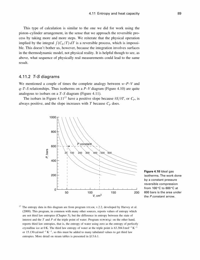
4.11 Entropy and heat capacity 89
This type of calculation is similar to the one we did for work using thepiston–cylinder arrangement, in the sense that we approach the reversible pro-cess by taking more and more steps. We reiterate that the physical operationimplied by the integral
∫�CP/T�dT is a reversible process, which is impossi-
ble. This doesn’t bother us, however, because the integration involves surfacesin the thermodynamic model, not physical reality. It is helpful though to see, asabove, what sequence of physically real measurements could lead to the sameresult.
4.11.2 T–S diagrams
We mentioned a couple of times the complete analogy between w–P–V andq–T–S relationships. Thus isotherms on a P–V diagram (Figure 4.10) are quiteanalogous to isobars on a T–S diagram (Figure 4.11).
The isobars in Figure 4.1117 have a positive slope because �S/�T , or CP, isalways positive, and the slope increases with T because CP does.
100 200 300 400 500 60025
V, cm3
P, b
ars
50 100 150 2000
200
400
600
800
1000
P constant
Figure 4.10 Ideal gasisotherms. The work doneby a constant pressurereversible compressionfrom 100 �C to 600 �C at600 bars is the area underthe P constant arrow.
17 The entropy data in this diagram are from program steam, v.2.2, developed by Harvey et al.(2000). This program, in common with many other sources, reports values of entropy whichare not third law entropies (Chapter 5), but the difference in entropy between the state ofinterest and the T and P of the triple point of water. Program supcrt92 on the other hand,reports third law entropies, that is, the entropy of water using zero as the entropy of perfectlycrystalline ice at 0K. The third law entropy of water at the triple point is 63.304 Jmol−1 K−1
or 15.130 calmol−1 K−1, so this must be added to many tabulated values to get third lawentropies. More detail on steam tables is presented in §13.6.1.
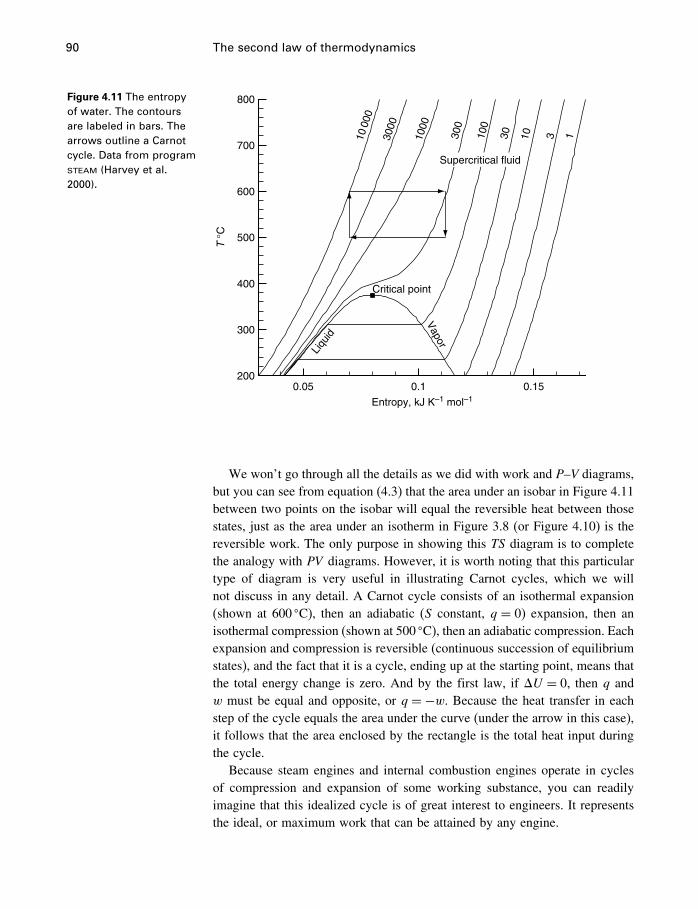
90 The second law of thermodynamics
Figure 4.11 The entropyof water. The contoursare labeled in bars. Thearrows outline a Carnotcycle. Data from programsteam (Harvey et al.2000).
Entropy, kJ K–1 mol–1
T°C
0.05 0.1 0.15200
300
400
500
600
700
800
Critical point
Vapor
Liqu
id
1000
0
3000
1000
300
100
30 10 3 1
Supercritical fluid
We won’t go through all the details as we did with work and P–V diagrams,but you can see from equation (4.3) that the area under an isobar in Figure 4.11between two points on the isobar will equal the reversible heat between thosestates, just as the area under an isotherm in Figure 3.8 (or Figure 4.10) is thereversible work. The only purpose in showing this TS diagram is to completethe analogy with PV diagrams. However, it is worth noting that this particulartype of diagram is very useful in illustrating Carnot cycles, which we willnot discuss in any detail. A Carnot cycle consists of an isothermal expansion(shown at 600 �C), then an adiabatic (S constant, q = 0) expansion, then anisothermal compression (shown at 500 �C), then an adiabatic compression. Eachexpansion and compression is reversible (continuous succession of equilibriumstates), and the fact that it is a cycle, ending up at the starting point, means thatthe total energy change is zero. And by the first law, if �U = 0, then q andw must be equal and opposite, or q = −w. Because the heat transfer in eachstep of the cycle equals the area under the curve (under the arrow in this case),it follows that the area enclosed by the rectangle is the total heat input duringthe cycle.
Because steam engines and internal combustion engines operate in cyclesof compression and expansion of some working substance, you can readilyimagine that this idealized cycle is of great interest to engineers. It representsthe ideal, or maximum work that can be attained by any engine.
4.12 A more useful thermodynamic potential 91
4.12 A more useful thermodynamic potential
Now we have two parameters, SU�V and US�V , that will tell us which wayprocesses will go, but they refer to processes which virtually never occur, exceptperhaps in classroom exercises – that is, processes which occur at constantvalues of U and V , or of S and V , our two constraints. We need a parameterwhich will refer to processes at constant T and P, our most common case.18
4.12.1 Gibbs energy
From Equation (4.19) (in the molar form),
dU −T dS+P dV ≤ 0 (4.34)
we can see that if we define a function
G= U −TS+PV (4.35)
called the Gibbs energy or the Gibbs free energy, the differential of which is
dG= dU −T dS−S dT +P dV +V dP (4.36)
or
dGT�P = dU −T dS+P dV (4.37)
Reversible versus irreversible compression
The reversible compression shown in Figure 4.10 looks very much like the
irreversible compression shown in Figure 3.9, but it is quite different. In Figure 3.9
the initial and final states are at the same temperature. The compression is
irreversible, and any amount of work and heat exchange can occur, depending on
the weight on the piston. No isotherms can be shown, because this would imply
that we knew the temperature at all points on the compression arrow, but we
don’t. In Figure 4.10 the initial and final temperatures are different, and during
the compression the temperature is indicated by the isotherms. It is an example
of Equation (3.6).
18 It is usual to speak of processes occurring at constant U and V , or constant T and P. It wouldbe more accurate to speak of processes having the same values of U and V , or of T and P,before and after the process. It doesn’t really matter what the system does between the twostates; that is, the system need not be at constant T and P during the process.
92 The second law of thermodynamics
which, combined with (3.16), is
dGT�P = dH−T dS (4.38)
then we find by comparing (4.37) and (4.34) that
dGT�P ≤ 0 (4.39)
Thus our definition of the second law has led to a function, G, which willalways decrease to a minimum in spontaneous processes in systems havingspecified values of T and P. It is an extremely useful thermodynamic potential.All we have to do is to find a way to get measurable values of this function forall pure compounds and solutes, and to find how they change with T , P, andconcentration, and we will then be able to predict the equilibrium configurationof any system by minimizing G.
To see how G changes with T and P is fairly simple. To see how it changeswith composition is a little more difficult (see §§7.6; 8.2). Combining (4.9)and (4.36), we find another fundamental equation,19
dG=−S dT +V dP (4.40)
Because (4.40) could also be written as a total differential,
dG=(�G
�T
)P
dT +(�G
�P
)T
dP (4.41)
we see from (4.40) that
��G/�T�P =−S (4.42)
and
��G/�P�T = V (4.43)
which are the slopes of the G–T–P surface in the T and P directions(Figure 4.9b). We will see how to integrate these expressions shortly.
In addition,
dGT�P = 0 (4.44)
Equation (4.44) is simply the condition for a minimum in G, that is, the tangentis horizontal (see Figure 4.14). It follows too, that �GT�P < 0 for spontaneousprocesses in systems having the same T and P before and after the process,
19 Equation (4.40) is derived in a more mathematically elegant way in §C.4. It is more elegantbecause it shows in a simple way how all thermodynamic potentials are intimately related.
4.12 A more useful thermodynamic potential 93
because any spontaneous process must head toward this minimum from somehigher point (some point of greater G value).20
The total form of Equation (4.36) is
dG= dU−T dS−SdT +P dV+VdP (4.45)
and combining this with Equation (4.14), we get
dG=−SdT +VdP−�d� (4.46)
which is analogous to (4.14), and so can be written
dG=−SdT︸ ︷︷ ︸heat
+ VdP︸ ︷︷ ︸PV work
− �d�︸ ︷︷ ︸chemical work︸ ︷︷ ︸
work
(4.47)
Gibbs energy in chemical reactionsLet’s review what we know about Equation (4.46). The dG = −SdT +VdPpart describes an equilibrium surface in GTP space for a particular system.Recalling the discussion in §4.8.1, dG = −SdT +VdP describes either thestable equilibrium surface or a metastable equilibrium surface. Its just that thefunctional relationship between S and T and between V and P will be differentin the two cases. In other words, you can apply dG=−SdT +VdP to eithercalcite or aragonite.
When the third constraint is added, as in Equation (4.46), the dG=−SdT+VdP part of the equation normally refers to the stable equilibrium surface. The�d� part then represents chemical work, such as the work you would obtainby discharging the battery (or changing aragonite to calcite), and so representsthe difference in G between the two surfaces.21
The equation thus opens the way to considering chemical reactions tryingto achieve stable equilibrium, not just the equilibrium states themselves, andwould therefore appear to be extremely important. Well, it is, but perhaps notas much as you might think. In Chapter 18 we will show how to use thequantity �d� in considering chemical reactions, but in fact calculating thevalue of � is not usually required. Using the progress variable � itself is quitecommon, but although implicitly linked to �, this link is not necessarily madeexplicit in calculations.
20 Note that the mathematical conditions for a function minimum, such as dUS�V = 0 anddGT�P = 0, are all true simultaneously at the minimum, as illustrated in Figure 4.5, and theyimply nothing whatsoever about how the function (i.e., the system) reached or achieved thatminimum.
21 It is conceivable that the “dG=−SdT +VdP part of the equation” could refer to ametastable state or surface, in which case the “�d� part” would represent the work ofcharging the battery or changing calcite to aragonite, but in fact it is never used in this sense.
94 The second law of thermodynamics
4.12.2 Helmholtz energy
Similarly, if we define a function
A= U −TS (4.48)
called the Helmholtz energy, or the Helmholtz work function, the differentialof which is
dA= dU −T dS−S dT (4.49)
or
dAT = dU −T dS (4.50)
we find, comparing (4.34) and (4.50),
dAT +P dV ≤ 0 (4.51)
or
dAT�V ≤ 0 (4.52)
Thus we have another function, A, which will always decrease to a minimumin spontaneous processes in systems having specified values of T and V , andis another thermodynamic potential. The usefulness of this function will bediscussed below.
4.13 Gibbs and Helmholtz functions as work
4.13.1 Gibbs energy as useful work
A ball in a metastable equilibrium valley (e.g., Figure 1.2) is capable of doingwork as it rolls down to lower elevations (once it is pushed over the barrier).The maximum work it can do is exactly equal to the (minimum) work requiredto push the ball back up to its metastable elevation. One way of understandingthe Gibbs energy is that it is equal to the maximum amount of useful workthat chemical systems can do as they change from metastable states to stablestates, underlining the usefulness of the ball-in-valley analogy.
However, we must first distinguish between total work and useful work.Chemical systems undergoing change (i.e., in which reactions occur) can dovarious kinds of work. For instance, batteries can do electrical work. Whileundergoing these reactions, the chemical system invariably has some changein volume, because it is most unlikely that the reaction products would haveexactly the same volume as the reactants. This change in volume �V takesplace under some ambient pressure P, so that P �V work is done during the
4.13 Gibbs and Helmholtz functions as work 95
reaction regardless of whether any other kind of work is done or not – ifthe reaction is to take place, it cannot be avoided. This “work against theatmosphere” (or against the confining pressure, whatever it is) usually is notuseful; it simply takes place whether we like it or not, and at atmosphericpressure it is often a rather small part of the total energy change. Althoughwe can decide to eliminate electrical work or other kinds of mechanical workfrom our systems, we cannot eliminate this P �V work (unless we consideronly constant volume systems, which is not usually very practical). We cantalk about the total work w, or the total work per mole, w. Net work (per mole)other than P �V work can be written
wnet = �wtotal−wP�V �= �w+P �V�
and because q ≤ T �S (integration of Equation 4.3), it follows from the firstlaw (�U = q+w) that
w ≥ �U −T �S (4.53)
Adding P �V to both sides,
w+P �V ≥ �U −T �S+P �V
and so
wnet ≥ �U −T �S+P �V (4.54)
Now,
G= U −TS+PVdG= dU −T dS−S dT +P dV −V dP
dGT�P = dU −T dS+P dV (4.55)
and
�GT�P = �U −T �S+P �V (4.56)
So, combining (4.54) and (4.56),
wnet ≥ �GT�P (4.57)
or, the other way around,
�GT�P ≤ wnet
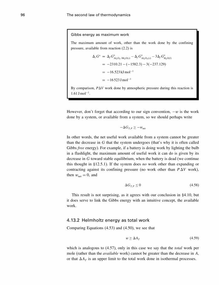
96 The second law of thermodynamics
Gibbs energy as maximum work
The maximum amount of work, other than the work done by the confining
pressure, available from reaction (2.2) is
�rG� = �fG
�Al2O3·3H2O�s�
−�fG�Al2O3�s�
−3�fG�H2O�l�
= −2310�21− �−1582�3�−3�−237�129�
= −16�523kJmol−1
= −16523 Jmol−1
By comparison, P�V work done by atmospheric pressure during this reaction is
1.61 Jmol−1.
However, don’t forget that according to our sign convention, −w is the workdone by a system, or available from a system, so we should perhaps write
−�GT�P ≥−wnet
In other words, the net useful work available from a system cannot be greaterthan the decrease in G that the system undergoes (that’s why it is often calledGibbs free energy). For example, if a battery is doing work by lighting the bulbin a flashlight, the maximum amount of useful work it can do is given by itsdecrease in G toward stable equilibrium, when the battery is dead (we continuethis thought in §12.5.1). If the system does no work other than expanding orcontracting against its confining pressure (no work other than P �V work),then wnet = 0, and
�GT�P ≤ 0 (4.58)
This result is not surprising, as it agrees with our conclusion in §4.10, butit does serve to link the Gibbs energy with an intuitive concept, the availablework.
4.13.2 Helmholtz energy as total work
Comparing Equations (4.53) and (4.50), we see that
w ≥ �AT (4.59)
which is analogous to (4.57), only in this case we say that the total work permole (rather than the available work) cannot be greater than the decrease in A,or that �AT is an upper limit to the total work done in isothermal processes.
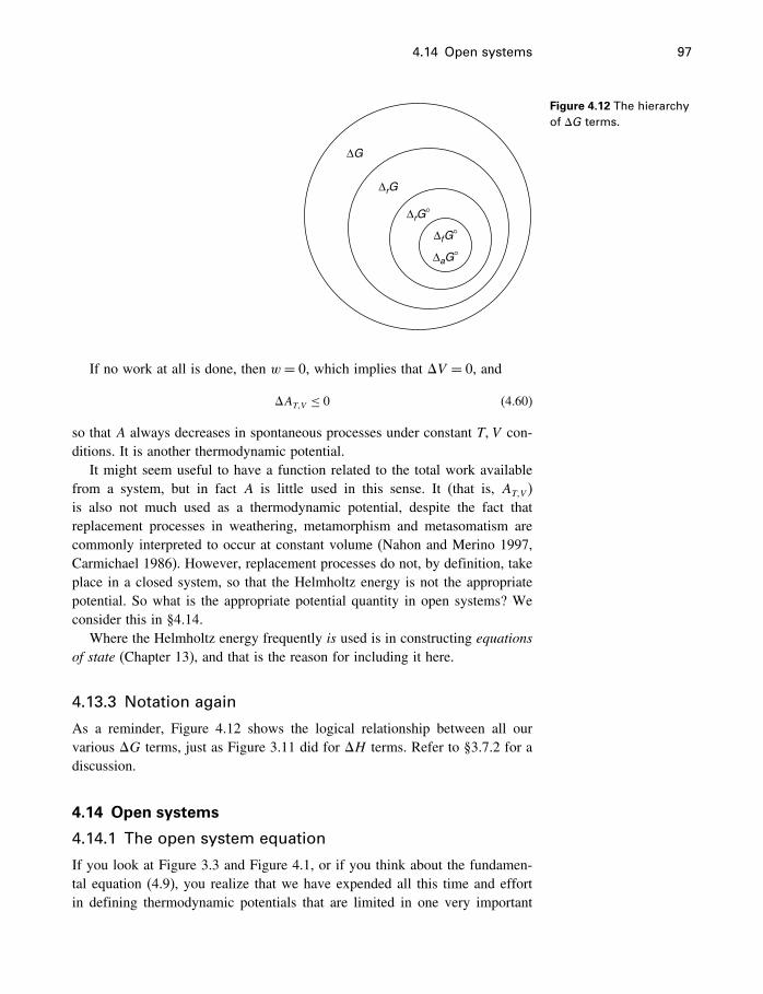
4.14 Open systems 97
∆G
∆rG
∆rG°
∆aG°
∆fG°
Figure 4.12 The hierarchyof �G terms.
If no work at all is done, then w = 0, which implies that �V = 0, and
�AT�V ≤ 0 (4.60)
so that A always decreases in spontaneous processes under constant T�V con-ditions. It is another thermodynamic potential.
It might seem useful to have a function related to the total work availablefrom a system, but in fact A is little used in this sense. It (that is, AT�V )is also not much used as a thermodynamic potential, despite the fact thatreplacement processes in weathering, metamorphism and metasomatism arecommonly interpreted to occur at constant volume (Nahon and Merino 1997,Carmichael 1986). However, replacement processes do not, by definition, takeplace in a closed system, so that the Helmholtz energy is not the appropriatepotential. So what is the appropriate potential quantity in open systems? Weconsider this in §4.14.
Where the Helmholtz energy frequently is used is in constructing equationsof state (Chapter 13), and that is the reason for including it here.
4.13.3 Notation again
As a reminder, Figure 4.12 shows the logical relationship between all ourvarious �G terms, just as Figure 3.11 did for �H terms. Refer to §3.7.2 for adiscussion.
4.14 Open systems
4.14.1 The open system equation
If you look at Figure 3.3 and Figure 4.1, or if you think about the fundamen-tal equation (4.9), you realize that we have expended all this time and effortin defining thermodynamic potentials that are limited in one very important
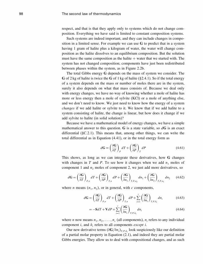
98 The second law of thermodynamics
respect, and that is that they apply only to systems which do not change com-position. Everything we have said is limited to constant composition systems.
Such systems are indeed important, and they can include changes in compo-sition in a limited sense. For example we can use G to predict that in a systemhaving 1 gram of halite plus a kilogram of water, the water will change com-position as the halite dissolves to an equilibrium composition. But the solutionmust have the same composition as the halite + water that we started with. Thesystem has not changed composition; components have just been redistributedbetween phases within the system, as in Figure 2.2b.
The total Gibbs energy G depends on the mass of system we consider. TheG of 2 kg of halite is twice the G of 1 kg of halite (§2.4.1). So if the total energyof a system depends on the mass or number of moles there are in the system,surely it also depends on what that mass consists of. Because we deal onlywith energy changes, we have no way of knowing whether a mole of halite hasmore or less energy then a mole of sylvite (KCl) or a mole of anything else,and we don’t need to know. We just need to know how the energy of a systemchanges if we add halite or sylvite to it. We know that if we add halite to asystem consisting of halite, the change is linear, but how does it change if weadd sylvite to halite (in solid solution)?
Because we have a mathematical model of energy changes, we have a simplemathematical answer to this question. G is a state variable, so dG is an exactdifferential (§C.2.1). This means that, among other things, we can write thetotal differential as in Equation (4.41), or in the total energy form as
dG=(�G�T
)P
dT +(�G�P
)T
dP (4.61)
This shows, as long as we can integrate these derivatives, how G changeswith changes in T and P. To see how it changes when we add n1 moles ofcomponent 1 and n2 moles of component 2, we just add more derivatives, so
dG=(�G�T
)P�n
dT +(�G�P
)T�n
dP+(�G�n1
)T�P�n2
dn1+(�G�n2
)T�P�n1
dn2 (4.62)
where n means �n1� n2�, or in general, with c components,
dG=(�G�T
)P�n
dT +(�G�P
)T�n
dP+c∑i=1
(�G�ni
)T�P�ni
dni (4.63)
=−SdT +VdP+c∑i=1
(�G�ni
)T�P�ni
dni (4.64)
where n now means n1� n2� � nc (all components), ni refers to any individualcomponent i, and ni refers to all components except i.
Our new derivative terms ��G/�ni�T�P�ni look suspiciously like our definitionof a partial molar property in Equation (2.1), and indeed they are partial molarGibbs energies. They allow us to deal with compositional changes, and as such
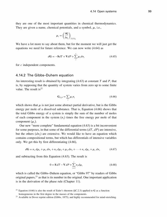
4.14 Open systems 99
they are one of the most important quantities in chemical thermodynamics.They are given a name, chemical potentials, and a symbol, �, i.e.,
�i =(�G�ni
)T�P�ni
We have a lot more to say about them, but for the moment we will just get theequations we need for future reference. We can now write (4.64) as
dG=−SdT +VdP+c∑i
�idni (4.65)
for c independent components.
4.14.2 The Gibbs–Duhem equation
An interesting result is obtained by integrating (4.63) at constant T and P, thatis, by supposing that the quantity of system varies from zero up to some finitevalue. The result is22
GT�P =∑i
�ini (4.66)
which shows that � is not just some abstract partial derivative, but is the Gibbsenergy per mole of a dissolved substance. That is, Equation (4.66) shows thatthe total Gibbs energy of a system is simply the sum of the number of molesof each component in the system (ni) times the free energy per mole of thatcomponent (�i).
Our new “more complete” fundamental equation (4.63) is a bit inconvenientfor some purposes, in that some of the differential terms (dT , dP) are intensive,but the others (dni) are extensive. We would like to have an equation whichcontains compositional terms, but which has differentials of intensive variablesonly. We get this by first differentiating (4.66),
dG= n1 d�1+�1 dn1+n2 d�2+�2 dn2+· · ·+nc d�c+�c dnc (4.67)
and subtracting from this Equation (4.63). The result is
0= SdT −VdP+c∑i=1
nid�i (4.68)
which is called the Gibbs–Duhem equation, or “Gibbs 97” by readers of Gibbsoriginal papers,23 as that is its number in the original. One important applicationis in the derivation of the phase rule (Chapter 11).
22 Equation (4.66) is also the result of Euler’s theorem (§C.2.3) applied to G as a functionhomogeneous in the first degree in the masses of the components.
23 Available in Dover reprint edition (Gibbs, 1875), and highly recommended for mind-stretching.
100 The second law of thermodynamics
The integrated formAnother important application of this equation is to show that even thoughthe components in the system are compositionally independent of one another,their chemical potentials are not always independent. In a binary solution ofcomponents 1 and 2, you can change n1 without changing n2, but doing thiswill change both �1 and �2. This turns out to be quite important in Chapter 10.Let’s see how it works.
At a constant T and P, Equation (4.68) becomesc∑i=1
nid�i = 0 (4.69)
so for a binary system
n1 d�1+n2 d�2 = 0 (4.70)
or, dividing by n1+n2,x1 d�1+x2 d�2 = 0 (4.71)
so
d�1 =−x2x1d�2 (4.72)
�′′1 −�′
1 =−∫ x′′1
x′1
x2x1d�2 (4.73)
showing that if you know how one potential changes as a result of a com-positional change, you can calculate the change in the other. They are notindependent.
This process can be extended to ternary or even higher order systems,and it can be shown that all chemical potentials in a multicomponent systemcan be evaluated if the potential of one component is known over the wholecompositional space. However, the process becomes complex, and has beenlittle used even in ternary systems. Pitzer and Brewer (1961, Chapter 34) havea discussion of this, with several useful references. The vast majority of usesof the Gibbs–Duhem relation have been in binary systems, using variations ofEquation (4.73). We should mention that the term Gibbs–Duhem is commonlyapplied to any of Equations (4.68)–(4.73).
Equation (4.73) proves inconvenient in practice, because �→−� as x→ 0.That is, � changes very rapidly in dilute solutions and does not approach alimit, so it’s not convenient in integration. Equation (4.73) is therefore modifiedto a more convenient form, which we will see in Chapter 10.
4.14.3 Other kinds of open systems
The open system as a subsystem in an overall closed system (Figure 2.2b) isby far the most commonly used kind of open system in geochemistry. In any
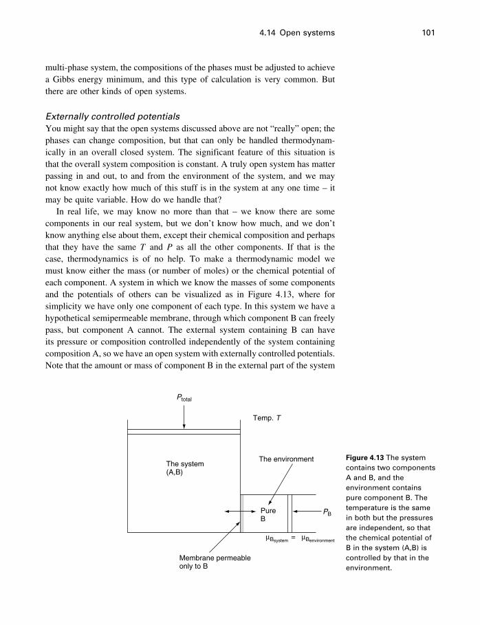
4.14 Open systems 101
multi-phase system, the compositions of the phases must be adjusted to achievea Gibbs energy minimum, and this type of calculation is very common. Butthere are other kinds of open systems.
Externally controlled potentialsYou might say that the open systems discussed above are not “really” open; thephases can change composition, but that can only be handled thermodynam-ically in an overall closed system. The significant feature of this situation isthat the overall system composition is constant. A truly open system has matterpassing in and out, to and from the environment of the system, and we maynot know exactly how much of this stuff is in the system at any one time – itmay be quite variable. How do we handle that?
In real life, we may know no more than that – we know there are somecomponents in our real system, but we don’t know how much, and we don’tknow anything else about them, except their chemical composition and perhapsthat they have the same T and P as all the other components. If that is thecase, thermodynamics is of no help. To make a thermodynamic model wemust know either the mass (or number of moles) or the chemical potential ofeach component. A system in which we know the masses of some componentsand the potentials of others can be visualized as in Figure 4.13, where forsimplicity we have only one component of each type. In this system we have ahypothetical semipermeable membrane, through which component B can freelypass, but component A cannot. The external system containing B can haveits pressure or composition controlled independently of the system containingcomposition A, so we have an open system with externally controlled potentials.Note that the amount or mass of component B in the external part of the system
PureB
The environmentThe system(A,B)
Membrane permeableonly to B
Temp. T
PB
Ptotal
µBsystem= µBenvironment
Figure 4.13 The systemcontains two componentsA and B, and theenvironment containspure component B. Thetemperature is the samein both but the pressuresare independent, so thatthe chemical potential ofB in the system (A,B) iscontrolled by that in theenvironment.
102 The second law of thermodynamics
is irrelevant. The use of such a “magical membrane” to model our system mayseem bothersome to some. We can address this in two ways.
• There actually are such membranes in common use in experimental work. Platinum at
high temperatures is permeable to hydrogen but not to other substances, and this fact
is extensively used to control the oxidation state of experiments. This is discussed
further in §11.5.2.• Real geological systems have no such membranes, but they do have components
(e.g. H2O) which have externally controlled potentials, such as practically any rock
undergoing hydrothermal alteration, and the membrane allows us to model this situ-
ation. The fact that the model system has a membrane but the real system does not is
no more important than many other differences between the two kinds of systems.
The question is, what thermodynamic potential is appropriate to this situa-tion? It cannot be the Gibbs energy, because if we write (4.65) for componentsA and B, and consider T , P, and nA to be fixed, we get
dGT�P�nA= �B dnB
The closed system criterion for equilibrium is dGT�P = 0, but this is obviouslyinappropriate in this case because �B is certainly not zero and dnB is notnecessarily zero because we have said nothing about PB. There are in fact noconditions pertaining only to the system containing both A and B that willspecify the equilibrium state when the environment is attached to it. This isessentially self-evident. A thermodynamic potential appropriate for the systemplus environment must evidently contain terms referring to both parts of thesystem.
Thompson’s L functionThe thermodynamics of this situation was worked out independently byKorzhinskii (1959) and Thompson (1970). The easiest way to do this is by aLegendre transform (discussed in §C.4) of a potential already established forother parameters. Starting with
G=G�T�P�nA� nB�
we want a new function, which Thompson (1970) has called L, which preservesthe potential qualities of G but has different independent variables; i.e., wewant
L= L�T�P�nA��B�
We find the Legendre transform by subtracting from G the product of the oldvariable and the derivative of the old function with respect to that variable.Thus
L=G−nB(�G�nB
)
4.15 The meaning of entropy 103
or
L=G−nB�B (4.74)
Differentiating (4.74) and adding (4.65) written for components A and B, weget
dL=−SdT +VdP+�AdnA−nBd�B (4.75)
showing that L has �T�P�nA��B� as independent variables. L is a function thatis minimized at equilibrium for given values of T�P�nA and �B, in exactly thesame way that G is minimized for given values of T�P�nA and nB. Since nBis not zero, dL is clearly only zero when d�B is zero, which will of course bewhen �B is the same in the system and in the environment.
The L function has not found much use in geochemistry to date, and we willnot use it in this text. It is included here to demonstrate that thermodynamicscan in fact handle truly open systems, and because it is an interesting exercise inthe use of the Legendre transform. Also it seems quite posssible that inventivegeochemists will find much greater use for this (and other thermodynamicpotentials?) in the future. Its derivation and use in metamorphic studies hashad a somewhat troubled history, nicely reviewed and discussed by Rumble(1982).
Engineering applicationsOpen systems are much more common in mechanical engineering. Basicallythis is because the applications do not involve chemical reactions to nearly thesame extent. All kinds of heat engines, turbines, refrigeration machines, boilers,and so on can be modeled in terms of mass and energy balances. Conservation ofmass and energy in the inputs and outputs, which is basically the first law, plusheat to work conversion, the second law, account for much of thermodynamicmodeling in these applications. Mechanical engineering texts may not evenmention the concept of activity (Chapter 8), so central to geochemistry.
4.15 The meaning of entropy
As long as we are dealing with pure compounds, we have answered just aboutall our questions. We have an energy parameter, the Gibbs energy, whichalways decreases in spontaneous reactions at a given T and P, and we knowhow to measure this energy term – calorimetry. We know, however, that thisenergy term, �G, is made up partly of a fairly comprehensible term �H , whichis just a heat flow term, and another term �S, which is more mysterious. Allwe know about this one is that we defined the second law such that the entropyalways increases in spontaneous reactions in isolated systems. The entropy is
104 The second law of thermodynamics
not itself an energy term, but the product of T and S, or T and �S, is an energyterm.
If we had to rely on classical thermodynamics, we would know little morethan we have already said about entropy. It is a parameter, with a method ofmeasurement, which increases in spontaneous processes, even when no energychanges are possible, that is, in isolated systems. We would also notice, aftermeasuring the entropy of many substances, that the entropies of gases arerelatively large, those of solids relatively small, and those of liquids somewherein between, but we would probably not have any mental picture of what entropyrepresents physically.
If you look at some processes that are quite irreversible but that involvelittle or no energy change, such as the mixing of two gases or the spreadingof a colored dye in water, you observe a driving force for processes that isquite different from the energy-drop paradigm we have been pursuing (theball rolling downhill). There is no energy drop when gases mix, but they doso invariably and irreversibly, and this shows that another driving force forreactions is mixing, or an increase in “mixed-upness,” which will take place ifit is possible. If you think about gases as collections of countless tiny moleculeszipping around with the speed of rifle bullets, but with quite a lot of spacebetween them, you realize that if two different gases are brought together, itis no more difficult to understand why they will always mix together than it isto understand why a ball will roll downhill. But this mixing process involvesno energy change (at least for ideal gases), so the first law of thermodynamicsis powerless – it cannot be the basis for a thermodynamic explanation. Thesecond law and entropy do provide it. Entropy can be thought of as a degreeof mixed-upness, and increasing the randomness or mixed-upness of systemsis one of the driving forces for spontaneous reactions.
The confusion arises because it is not the only one – the ball rolling downthe hill (energy decrease) is also one. It is the two together that provide thecomplete answer. In some processes energy decrease is the dominant factor,and in others, mixing or entropy increase is the dominant factor. The two arebrought together in the Gibbs energy equation
dGT�P = dH−T dS [4.38]
which can also be written
�GT�P = �H−T �S
Here there are two factors that together determine whether �GT�P will bepositive or negative. One is �H�= �U +P �V�, which is the energy changedue to heat and work in the process represented by �, and the other is T �S,the energy change due to the mixing factor. In many spontaneous reactions,�H is negative (the process is exothermic) and �S is positive (mixed-upness
4.15 The meaning of entropy 105
increases), and so both factors are negative (T �S positive, −T �S negative)and �G is negative. In other reactions, �H is positive (process is endothermic,e.g., melting ice), but the �S term is sufficiently large and positive so thatT �S > �H , and �G is negative in spite of the positive �H . This will beespecially true at high temperatures, when T is large. There are all varietiesof combinations; the point is that whether or not any particular process isspontaneous is the result of the two competing factors. Systems want to lowertheir energy content, but they also want to maximize their mixed-upness. Thebalance between these factors decides the issue.
4.15.1 But what is entropy, really?
This question has been around since Clausius invented the term in 1865,and the answer takes on many forms. Some follow the historical route, fromsteam engines, to Carnot, Clausius, Thompson, Joule, Rankine, and so on.A particularly lucid, concise account of this history is Purrington (1997).A central feature of this approach is Carnot cycles, as used by Clausius todeduce the existence of the entropy parameter. This approach is rather abstract,and needs some manipulation to be seen to be connected to thermodynamicpotentials and chemical reactions. Others emphasize the impossibility of someprocesses, or the “availability” of energy, and some have a rather uniqueviewpoint, such as Reiss (1965), who considers entropy as the “degree ofconstraint.”
Virtually since the beginning, however, a popular viewpoint has been tosee entropy as a measure of disorder. Helmholtz used the word “Unordnung”(disorder) in 1882. This results from familiar relationships such as Sgases >Sliquids > Ssolids, and the universally positive entropy of mixing. We used thisrelationship in the previous section when we spoke of “degree of mixed-upness.” However the “disorder” analogy can involve a serious fallacy, as madeclear by Lambert (1999; see also http://www.entropysite.com).
The rather subjective concepts of disorder and mixed-upness are usefulanalogies in certain situations, such as melting solids and mixing gases, butthey fail completely in most other situations. You cannot tell whether - or�-quartz is “more disordered” or has the higher entropy by looking at theirstructures. Shuffling a deck of cards perhaps increases its disorder, but it doesnot increase the entropy of the cards. To see this, just imagine cooling the cardsdown to near zero K, measuring their heat capacity up to room temperature, anddetermining the entropy of the card deck from these measurements. Obviously,the result will be the same no matter in what state of order the cards are. Thesame is true for the configuration of any macroscopic system. Checkers on aboard are ordered at the start of a game, and become progressively disorderedduring a game, but the entropy of the checkers remains the same no matterwhat their arrangement.
106 The second law of thermodynamics
A complete understanding of this inevitably involves statistical and evensome quantum mechanics. In statistical mechanics, the atoms in a system arepostulated to have a number of “microstates,” which are energetic states of thesystem, the definition of which involves the distribution of energy quanta overavailable energy levels in the particles in a macroscopic system. If a changeoccurs so as to increase the number of available microstates, energy will spreadout among the newly available microstates. The basic postulate of statisticalmechanics is that over long periods of time, every possible microstate of anisolated assembly occurs with equal probability (Nash, 1972). The quantity Win the famous Boltzmann–Planck equation
S= k lnWis in fact the number of these microstates, where W = 1 for a perfect crystal atabsolute zero K and k is Boltzmann’s constant (which, significantly, includestemperature). The stable state simply has an immensesly greater number ofequivalent microstates.
Much of the discussion in statistical mechanics concerns probability dis-tributions and their application to microstates. Information theory (Shannon,1949) defines a quantity −∑i pi logpi, called the entropy of a probability dis-tribution, which has some remarkable similarities to the properties of classicalor thermodynamic entropy. What seems to be overlooked by nonexperts isthat in chemistry and physics, the probability distributions being discussed arethose of energy distributions among microstates. When we speak of mixing or“mixed-upness,” we actually refer to particles (atoms, molecules) distributingthemselves in different energetic states, not to macroscopic things like cards orcheckers. Explaining entropy does involve probability theory, but the proba-bilities refer to energetic states, not to the outcome of dealing cards or tossingdice.
The central fact about entropy as used in science is that it involves thedistribution of energy in a system. Energy tends to become “spread out,” ordelocalized, if not prevented from doing so. The “configurational entropy”much used by mineralogists in discussing the various arrangements of atoms ona crystal lattice (Chapter 14) is fundamentally different fom the arrangement ofcheckers on a board because energy is transferred when atomic arrangementsare changed – the heat capacity of each arrangement is different.
If you “really” want to understand entropy, you need to learn more thanjust equilibrium thermodynamics. In this book, we take the simple view thatentropy is a parameter, having a clearly defined method of measurement, whichenables us to define thermodynamic potentials in chemical systems. It is simplyrelated to “disorder” in many simple situations, which is an intuitive aid, butthis aid doesn’t extend very far. Because of this resemblance to probability anddisorder, entropy has been related to everything from shuffled cards to the fallof empires, but these connections for the most part have nothing to do with thesecond law of thermodynamics.
4.17 The end of the road 107
4.16 A word about Carnot
Some readers may have noticed that, despite the numerous equations and deriva-tions, the introduction of entropy and the second law is less than completelyrigorous in this chapter. This is because at a crucial point, the introduction ofthe relationship between entropy, temperature, and heat (Equation 4.3), we relyon analogy rather than demonstration or argument. Most treatments rely on adiscussion of Carnot cycles, but as one chemist has observed,
Arguments based on heat engines have little appeal to chemists
(McGlashan, 1979, p. 111).
In my experience, such arguments have even less appeal to geochemists. Thisis perhaps unfortunate, because approaching the subject from various points ofview certainly aids understanding, and in fact the heat engine approach is veryuseful in the derivation of Equation (4.3), and also the kelvin temperature scale.
However, such discussions tend to be rather long and abstract, and exactlyhow conclusions about irreversible heat transfers in Carnot cycles get trans-ferred to irreversibility in chemical reactions requires even more discussion.This detracts from the task attempted here – the shortest possible, intuitivelyclear, development of the concepts necessary to use thermodynamics in solvingEarth science problems. Readers who want to know more about the historicaldevelopment of the entropy concept and its deeper meaning must consult themany excellent treatises on this subject.
4.17 The end of the road
We pause here to note that, in case you hadn’t noticed, we have arrived atthe answer to the question posed in Chapters 1 and 2. The question was, whatcontrols whether a reaction or a process will happen or not happen? Why doeswater freeze below 0 �C and ice melt above 0 �C?What is the “chemical energy”term that always decreases to a minimum, like the ball rolling down the hill? Inanswering this question, we first had to define fairly carefully some terminologysuch as system, equilibrium, and process. We then noted (Chapter 3) thatsystems have fixed energy contents (U, or U ) at equilibrium, but this didn’thelp, because although this energy is conserved, it doesn’t distinguish at allbetween directions processes take (bricks could cool themselves, and use thisenergy to fly, as far as U is concerned).
The missing ingredient to understanding why reactions go one way and notthe other is entropy. Entropy is defined as a state variable that always increasesin spontaneous processes in isolated systems. But a parameter that is usefulonly in isolated systems is not of much practical use, so we defined anotherstate variable, the Gibbs energy, that always decreases in spontaneous processin systems at a given T and P (see Figure 4.14). This is the parameter wehave been looking for. Figure 4.14 shows two different states of a system at
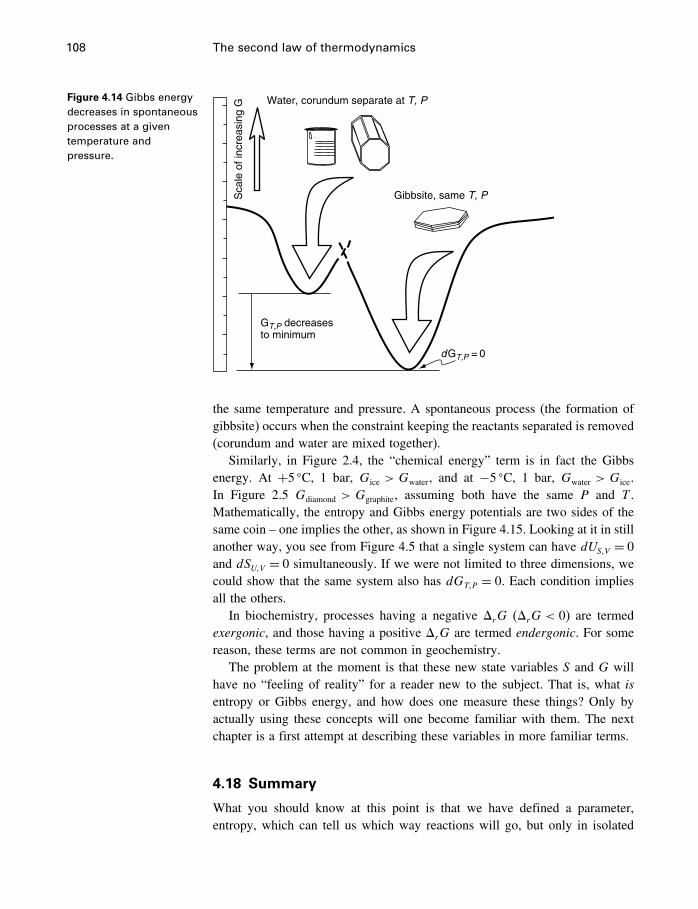
108 The second law of thermodynamics
Figure 4.14 Gibbs energydecreases in spontaneousprocesses at a giventemperature andpressure.
Water, corundum separate at T, P
Sca
le o
f inc
reas
ing
G
Gibbsite, same T, P
GT,P decreasesto minimum
dGT,P = 0
the same temperature and pressure. A spontaneous process (the formation ofgibbsite) occurs when the constraint keeping the reactants separated is removed(corundum and water are mixed together).
Similarly, in Figure 2.4, the “chemical energy” term is in fact the Gibbsenergy. At +5 �C, 1 bar, Gice > Gwater, and at −5 �C, 1 bar, Gwater > Gice.In Figure 2.5 Gdiamond > Ggraphite, assuming both have the same P and T .Mathematically, the entropy and Gibbs energy potentials are two sides of thesame coin – one implies the other, as shown in Figure 4.15. Looking at it in stillanother way, you see from Figure 4.5 that a single system can have dUS�V = 0and dSU�V = 0 simultaneously. If we were not limited to three dimensions, wecould show that the same system also has dGT�P = 0. Each condition impliesall the others.
In biochemistry, processes having a negative �rG (�rG < 0) are termedexergonic, and those having a positive �rG are termed endergonic. For somereason, these terms are not common in geochemistry.
The problem at the moment is that these new state variables S and G willhave no “feeling of reality” for a reader new to the subject. That is, what isentropy or Gibbs energy, and how does one measure these things? Only byactually using these concepts will one become familiar with them. The nextchapter is a first attempt at describing these variables in more familiar terms.
4.18 Summary
What you should know at this point is that we have defined a parameter,entropy, which can tell us which way reactions will go, but only in isolated
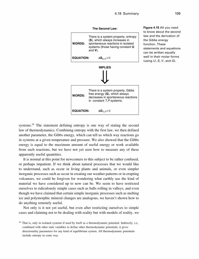
4.18 Summary 109
The Second Law:
IMPLIES
WORDS:
EQUATION:
There is a system property, entropy(S), which always increases inspontaneous reactions in isolatedsystems (those having constant Uand V).
∆SU,V ≥ 0
WORDS:
EQUATION:
There is a system property, Gibbsfree energy (G), which alwaysdecreases in spontaneous reactionsin constant T,P systems.
∆GT,P ≤ 0
Figure 4.15 All you needto know about the secondlaw and the derivation ofthe Gibbs energyfunction. Thesestatements and equationscan be written equallywell in their molar forms(using U, S, V , and G).
systems.24 The statement defining entropy is one way of stating the secondlaw of thermodynamics. Combining entropy with the first law, we then definedanother parameter, the Gibbs energy, which can tell us which way reactions goin systems at a given temperature and pressure. We also showed that the Gibbsenergy is equal to the maximum amount of useful energy or work availablefrom such reactions, but we have not yet seen how to measure any of theseapparently useful quantities.
It is normal at this point for newcomers to this subject to be rather confused,or perhaps impatient. If we think about natural processes that we would liketo understand, such as occur in living plants and animals, or even simplerinorganic processes such as occur in creating our weather patterns or in eruptingvolcanoes, we could be forgiven for wondering what earthly use the kind ofmaterial we have considered up to now can be. We seem to have restrictedourselves to ridiculously simple cases such as balls rolling in valleys, and eventhough we have claimed that certain simple inorganic processes such as meltingice and polymorphic mineral changes are analogous, we haven’t shown how todo anything remotely useful.
Not only is it not yet useful, but even after restricting ourselves to simplecases and claiming not to be dealing with reality but with models of reality, we
24 That is, only in isolated systems if used by itself as a thermodynamic potential. Indirectly, i.e.,combined with other state variables to define other thermodynamic potentials, it givesdirectionality parameters for any kind of equilibrium system. All thermodynamic potentialsinclude entropy in some way.
110 The second law of thermodynamics
have introduced at least one concept (entropy) that is rather difficult to fullycomprehend and have used a level of mathematics that, although not exceedingthat taught in introductory calculus courses, has physical implications that arehard to grasp. The best remedy for this is to review the material to some extent,and to plunge ahead even if it is not entirely clear. After some familiaritywith practical applications is attained, some of the earlier material will becomeclearer, so the best approach is continuous review, in addition to assimilationof new material.
It may well seem that we have made no progress toward understandingcomplex processes, but this is not true. Most natural processes are so complexthat we simply must start with the very simplest ones we can think of and defineour terms very carefully. Our goal of finding the secret to why reactions go inone direction and not the other may seem overly simple, but it is in fact the basicconcept necessary to build up an understanding of all the natural phenomenamentioned above. Of course, even when we have mastered thermodynamics,we will find that we don’t have all the answers to all our questions; in fact,we will find that the things thermodynamics can tell us are fairly limited. Theyhave, however, a level of certainty which surpasses that of most other waysof looking at the same problems, and this makes the subject an absolutelyessential element of all research into problems that involve energy transfers.You may wish to know much more than thermodynamics can tell you, but youneed to know what it can tell you.
5Getting data
5.1 Introduction
We have had quite enough theoretical discussion for now. Let’s see how toget some numbers into our equations so as to be able to calculate somethinguseful. Welcome to the world of experimental thermochemistry.
In this chapter we will have a look at a few of the ways in which thethermodynamic parameters we have derived are measured; i.e., where thenumbers in the tables and databases come from. A deep knowledge of thissubject is not necessary in order to use thermodynamics to model chemical,geological, or environmental systems, in the same sense that a knowledge ofa composer’s life and times is not necessary to enjoy his or her music. Butit does enrich the experience, and in the case of using thermodynamics, suchknowledge does serve to make the user conscious of the many, many reasonswhy his or her data might be incorrect. It enables the user to truly believe inthe “modeler’s motto” – never trust your data absolutely.
Thermochemical data are produced for the most part by dedicated scien-tists, who devote a good part of their lives to tracking down elusive sourcesof error, and devising ever-improved methods for determining nature’s fun-damental parameters as defined by thermodynamic theory. When determinedby independent methods and/or independent laboratories, the results are oftensatisfyingly in agreement, but almost as often they are not, meaning that thereis some source of error, and identifying it can take a lot of discussion (perhapsarguments would be a better term) and a long time.
Beginning with the establishment of the Geophysical Laboratory inWashington in 1905, scientists primarily interested in geological processeshave contributed to our knowledge of these thermodynamic properties, espe-cially, as might be expected, those of the rock and soil-forming minerals, andaqueous solutions such as sea water and hydrothermal solutions. In addition tothe measurement of mineral and solution properties, collecting these data intodatabases for use by computer programs, and the testing of these databases forinternal consistency has become increasingly important.
The experimental part and the self-consistent database part of using ther-modynamics in the Earth sciences today have both become large and complex
111
112 Getting data
subjects, each worthy of separate study. Geologists and geochemists primarilyinterested in Earth processes, but who need to do some thermodynamic mod-eling in order to better understand these processes, can be forgiven for notwanting to be involved with either experiment or database development. Nev-ertheless, rigorous thermodynamic methods can produce nonsensical results,given incorrect data, so a blind faith in the database attached to some computerprogram can be a recipe for disaster.
In this chapter (nor in this book) we cannot address these areas of study toany great extent, but understanding thermodynamics for most people is helpedby having some knowledge of how fundamental data are determined. The aimof this chapter is thus to trace the connection between laboratory experimentsand thermodynamic modeling. The idea is not only to impart some idea ofhow it is done, but some idea of the great difficulties involved at every stage,and therefore some respect for data. Good data are a precious commodity; youshould have some interest in where yours come from.
The discussion of methods in this chapter is very sketchy. Many details andvariations are omitted, because all we want to do is illustrate what is involved.Do not conclude from the simplicity of the presentation that there is nothingmuch to this experimental business. It is not too difficult to get data that arenot much good; it is extremely difficult, time consuming, frustrating and oftenexpensive, to get excellent data, ones that stand the test of time.1
Sections 5.2 to 5.7 deal primarily with obtaining data for solid phases.Section 5.8 deals with liquids, gases and solutes. An overview of many methodsused by Earth science experimenters can be found in Ulmer and Barnes (1987).
5.2 What to measure?
Imagine that you have an interesting field problem, and you want to do somethermodynamic modeling to better understand it, but for some reason there areno data for the mineral you are most interested in, gibbsite. You go to a fullyequipped laboratory, but what do you do there?
5.2.1 What not to do
Perhaps in your field study you have concluded that gibbsite is being formedfrom some other mineral by some alteration process you have figured out, and
1 Much the same can of course be said about field work, or indeed about any serious branch ofscience. If you don’t know much about it, it looks easy. I am reminded of the story of thegeochemist, well versed in theory and experiment, who said that field mapping could becarried out by a bunch of monkeys trained to collect samples. Let’s hope that such appallingignorance is not widespread.
5.2 What to measure? 113
you want to use thermodynamics to see if it makes sense. Maybe thermody-namics will tell you that this process is not permissible at your favorite T andP, or that gibbsite is not the stable phase.
But your alteration process involves other minerals, as well as an aqueoussolution. The most obvious thing to do then is to set up an experiment in whichyou try to duplicate this reaction. Perhaps you put some groundwater and someminerals together in some reaction vessel for a while, then look at the results.In other words, you try to duplicate nature. This approach has been tried manytimes, and generally the results are of very limited usefulness. The results areusually quite complex and difficult to interpret, and in any case they applyonly to one specific set of starting materials – it is difficult to draw generalconclusions from the results. Besides, the measurements you can make in suchexperiments, which are usually the compositions of some complex phases, havenothing to do with measuring heat and work, which as we have seen is thebasis of all our thermodynamic parameters.
5.2.2 What to do
If you wish to use thermodynamics, perhaps you should look at the equationsto get a clue as to what to measure. Looking at the first law, �U = q+w,you see that you will be involved in measuring heat and work. Looking at thesecond law, either dS = ∫ �CP/T�dT or �S = �H/T , you see that measuringheat at various temperatures is also involved. Measuring quantities associatedwith q and with w are therefore fundamental to experimental thermodynamics.There are quite a number of ways of doing this, but for the moment we candivide them into direct and indirect methods.
Direct methodsBased on our discussion so far, it seems that we would like most to know �rG
for reactions of interest to us, because this will tell us which way the reactionswill go, assuming that pressure and temperature are fixed. For example, if wewere not sure which of the two forms of carbon was the stable form at 25 �C,1 bar, we could measure Ggraphite−Gdiamond, which is �rG for the reaction
C�diamond�= C�graphite�
and if this quantity was negative, then graphite would be stable, and if it waspositive, diamond would be stable. The same reasoning would hold for anycomplex reaction involving gibbsite, as long as we know the Gibbs energy ofevery species in the reaction.
There are quite a number of ways of determining changes in Gibbs energy,but we will discuss only the most common one here. Others are associatedwith determining the equilibrium constant or cell voltages, as we will see in
114 Getting data
Chapters 9 and 12. To see how changes in G are measured, consider firstEquations (4.56) and (3.17)
�GT�P = �U −T �S+P �V [4.56]
�HP = �U +P �V [3.17]
Combining these, we have
�GT�P = �HP−T �S (5.1)
From this, we see that we can calculate �G for a process if we know �HPand �S for that process. We know (from §3.5) that �HP is simply the heattransferred to or from the closed system during a constant pressure process,so all we have to do is carry out some process (reaction) at some constant P,probably atmospheric P, and measure how much heat is evolved or absorbed.
This �H is also connected to �S, but only for a reversible process, aswe have seen. This might be a little difficult to do, experimentally. But wealso have an equation involving �S, CP and T (Equation 4.25), and CP isrelated to �H (Equation 3.25), so it begins to look like measuring heat ispretty important, even if you are not concerned with heat flow in your fieldsituation. Therefore, calorimetry, the art and science of measuring heat flows,is the secret to determining values of �G.
Indirect methodsSo far we have talked about using thermodynamics to determine phase relation-ships. But the opposite approach can also be used; phase relationships deter-mined under strictly controlled conditions (meaning controlled by the phaserule, Chapter 11) can be used to deduce fundamental thermodynamic proper-ties. For example, for gibbsite, you might conduct experiments to determinethe temperature at which gibbsite changes to corundum,
2Al�OH�3�s�= Al2O3�s�+3H2O�l� (5.2)
or, you might determine the solubility of gibbsite in water at various tempera-tures and pH values. Both these relationships are interesting to Earth scientistseven without thermodynamic manipulation, but they can also be used to deter-mine the thermodynamic properties of gibbsite and related species. This is asubject for later chapters, but intuitively it would seem that knowing the prop-erties of corundum and water, you might be able to deduce those for gibbsitefrom the requirement that reaction (5.2) be at equilibrium.
Even more importantly, families of such relationships, that is, a number ofrelationships involving the same minerals, can be used to test the consistencyof thermodynamic data. For example, suppose you have determined �fH
� foreach of gibbsite, corundum, and water from calorimetry. If you get a different
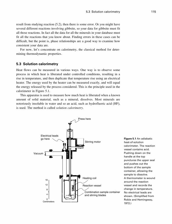
5.3 Solution calorimetry 115
result from studying reaction (5.2), then there is some error. Or you might haveseveral different reactions involving gibbsite, so your data for gibbsite must fitall those reactions. In fact all the data for all the minerals in your database mustfit all the reactions that you know about. Finding errors in these cases can bedifficult, but the point is, phase relationships are a good way to examine howconsistent your data are.
For now, let’s concentrate on calorimetry, the classical method for deter-mining thermodynamic properties.
5.3 Solution calorimetry
Heat flows can be measured in various ways. One way is to observe someprocess in which heat is liberated under controlled conditions, resulting in arise in temperature, and then duplicate that temperature rise using an electricalheater. The energy used by the heater can be measured exactly, and will equalthe energy released by the process considered. This is the principle used in thecalorimeter in Figure 5.1.
This apparatus is used to measure how much heat is liberated when a knownamount of solid material, such as a mineral, dissolves. Most minerals arenotoriously insoluble in water and so an acid, such as hydrofluoric acid (HF),is used. The method is called solution calorimetry.
Press here
Stirring motor
Heating coil
Reaction vessel
Combination sample containerand stirring blades
16
12
8
4
0Centimeters
Vacuum
Electrical leadsgo here Figure 5.1 An adiabatic
heat-of-solutioncalorimeter. The reactionvessel contains acid.Pushing down on thehandle at the toppunctures the upper sealand pushes out thebottom of the samplecontainer, allowing thesample to dissolve.A thermometer is woundaround the reactionvessel and records thechange in temperature.No electrical leads areshown. (Simplified fromRobie and Hemingway,1972.)
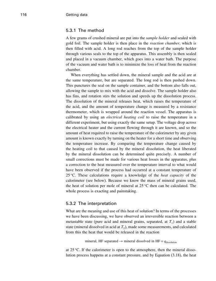
116 Getting data
5.3.1 The method
A few grams of crushed mineral are put into the sample holder and sealed withgold foil. The sample holder is then place in the reaction chamber, which isthen filled with acid. A long rod reaches from the top of the sample holderthrough various seals to the top of the apparatus. This assembly is then sealedand placed in a vacuum chamber, which goes into a water bath. The purposeof the vacuum and water bath is to minimize the loss of heat from the reactionchamber.
When everything has settled down, the mineral sample and the acid are atthe same temperature, but are separated. The long rod is then pushed down.This punctures the seal on the sample container, and the bottom also falls out,allowing the sample to mix with the acid and dissolve. The sample holder alsohas fins, and rotation stirs the solution and speeds up the dissolution process.The dissolution of the mineral releases heat, which raises the temperature ofthe acid, and the amount of temperature change is measured by a resistancethermometer, which is wrapped around the reaction vessel. The apparatus iscalibrated by using an electrical heating coil to raise the temperature in adifferent experiment, but using exactly the same setup. The voltage drop acrossthe electrical heater and the current flowing through it are known, and so theamount of heat required to raise the temperature of the calorimeter by any givenamount is known exactly by turning on the heater for a short time and observingthe temperature increase. By comparing the temperature change caused bythe heating coil to that caused by the mineral dissolution, the heat liberatedby the mineral dissolution can be determined quite precisely. A number ofsmall corrections must be made for various heat losses in the apparatus, plusa correction to the heat measured over the temperature interval to what wouldhave been observed if the process had occurred at a constant temperature of25 �C. These calculations require a knowledge of the heat capacity of thecalorimeter (see below). Because we know the mass of mineral grains used,the heat of solution per mole of mineral at 25 �C then can be calculated. Thewhole process is exacting and painstaking.
5.3.2 The interpretation
What are the meaning and use of this heat of solution? In terms of the processeswe have been discussing, we have observed an irreversible reaction between ametastable state (pure acid and mineral grains, separated, at T1) and a stablestate (mineral dissolved in acid at T2), made some measurements, and calculatedfrom this the heat that would be released in the reaction
mineral, HF separated→mineral dissolved in HF+qdissolutionat 25 �C. If the calorimeter is open to the atmosphere, then the mineral disso-lution process happens at a constant pressure, and by Equation (3.18), the heat
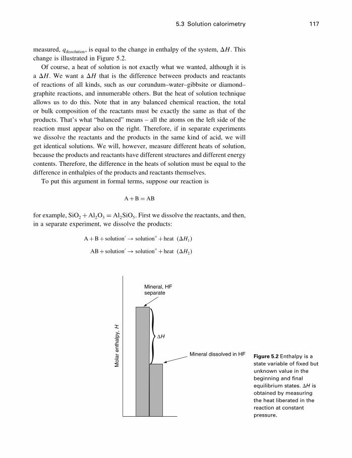
5.3 Solution calorimetry 117
measured, qdissolution, is equal to the change in enthalpy of the system, �H . Thischange is illustrated in Figure 5.2.
Of course, a heat of solution is not exactly what we wanted, although it isa �H . We want a �H that is the difference between products and reactantsof reactions of all kinds, such as our corundum–water–gibbsite or diamond–graphite reactions, and innumerable others. But the heat of solution techniqueallows us to do this. Note that in any balanced chemical reaction, the totalor bulk composition of the reactants must be exactly the same as that of theproducts. That’s what “balanced” means – all the atoms on the left side of thereaction must appear also on the right. Therefore, if in separate experimentswe dissolve the reactants and the products in the same kind of acid, we willget identical solutions. We will, however, measure different heats of solution,because the products and reactants have different structures and different energycontents. Therefore, the difference in the heats of solution must be equal to thedifference in enthalpies of the products and reactants themselves.
To put this argument in formal terms, suppose our reaction is
A+B= AB
for example, SiO2+Al2O3 = Al2SiO5. First we dissolve the reactants, and then,in a separate experiment, we dissolve the products:
A+B+ solution′ → solution′′ +heat ��H1�
AB+ solution′ → solution′′ +heat ��H2�
Mineral, HFseparate
∆H
Mineral dissolved in HF
Mol
ar e
ntha
lpy,
H
Figure 5.2 Enthalpy is astate variable of fixed butunknown value in thebeginning and finalequilibrium states. �H isobtained by measuringthe heat liberated in thereaction at constantpressure.
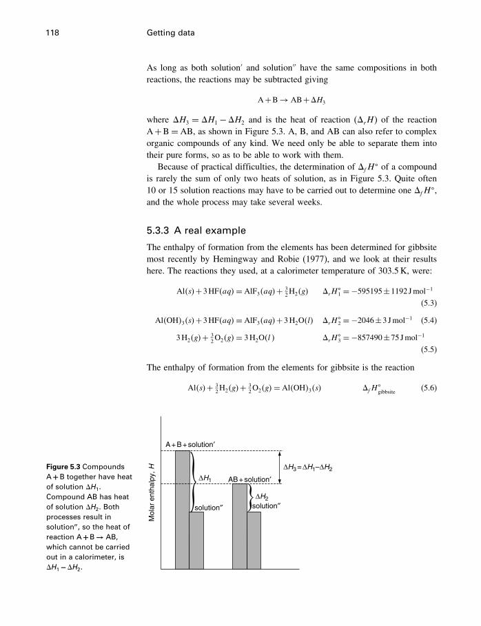
118 Getting data
As long as both solution′ and solution′′ have the same compositions in bothreactions, the reactions may be subtracted giving
A+B→ AB+�H3
where �H3 = �H1 −�H2 and is the heat of reaction (�rH) of the reactionA+B= AB, as shown in Figure 5.3. A, B, and AB can also refer to complexorganic compounds of any kind. We need only be able to separate them intotheir pure forms, so as to be able to work with them.
Because of practical difficulties, the determination of �fH� of a compound
is rarely the sum of only two heats of solution, as in Figure 5.3. Quite often10 or 15 solution reactions may have to be carried out to determine one �fH
�,and the whole process may take several weeks.
5.3.3 A real example
The enthalpy of formation from the elements has been determined for gibbsitemost recently by Hemingway and Robie (1977), and we look at their resultshere. The reactions they used, at a calorimeter temperature of 303.5K, were:
Al�s�+3HF�aq�= AlF3�aq�+ 32H2�g� �rH
�1 =−595195±1192 Jmol−1
(5.3)
Al�OH�3�s�+3HF�aq�= AlF3�aq�+3H2O�l� �rH�2 =−2046±3 Jmol−1 (5.4)
3H2�g�+ 32O2�g�= 3H2O�l � �rH
�3 =−857490±75 Jmol−1
(5.5)
The enthalpy of formation from the elements for gibbsite is the reaction
Al�s�+ 32H2�g�+ 3
2O2�g�= Al�OH�3�s� �fH�gibbsite
(5.6)
Figure 5.3 CompoundsA+B together have heatof solution �H1.Compound AB has heatof solution �H2. Bothprocesses result insolution′′, so the heat ofreaction A+B → AB,which cannot be carriedout in a calorimeter, is�H1 −�H2.
Mol
ar e
ntha
lpy,
H
A + B +solution′
solution″solution″
AB+solution′
∆H3 = ∆H1–∆H2
∆H1
∆H2
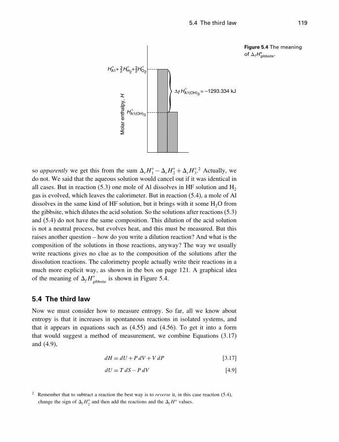
5.4 The third law 119
∆f HA1(OH)3= –1293.334 kJ°
HA1(OH)3°
HA1+ HH2+ HO2
32–
32–
° ° °
Mol
ar e
ntha
lpy,
H
Figure 5.4 The meaningof �f H
�gibbsite.
so apparently we get this from the sum �rH�1−�rH
�2+�rH
�3.2 Actually, we
do not. We said that the aqueous solution would cancel out if it was identical inall cases. But in reaction (5.3) one mole of Al dissolves in HF solution and H2
gas is evolved, which leaves the calorimeter. But in reaction (5.4), a mole of Aldissolves in the same kind of HF solution, but it brings with it some H2O fromthe gibbsite, which dilutes the acid solution. So the solutions after reactions (5.3)and (5.4) do not have the same composition. This dilution of the acid solutionis not a neutral process, but evolves heat, and this must be measured. But thisraises another question – how do you write a dilution reaction? And what is thecomposition of the solutions in those reactions, anyway? The way we usuallywrite reactions gives no clue as to the composition of the solutions after thedissolution reactions. The calorimetry people actually write their reactions in amuch more explicit way, as shown in the box on page 121. A graphical ideaof the meaning of �fH
�gibbsite
is shown in Figure 5.4.
5.4 The third law
Now we must consider how to measure entropy. So far, all we know aboutentropy is that it increases in spontaneous reactions in isolated systems, andthat it appears in equations such as (4.55) and (4.56). To get it into a formthat would suggest a method of measurement, we combine Equations (3.17)and (4.9),
dH = dU +P dV +V dP [3.17]
dU = T dS−P dV [4.9]
2 Remember that to subtract a reaction the best way is to reverse it, in this case reaction (5.4),change the sign of �fH
�2and then add the reactions and the �fH
� values.
120 Getting data
giving
dH = T dS+V dP (5.7)
If we choose constant pressure conditions, dP becomes zero, and substitutingCP dT for dH (Equation 3.23), we have
CP dT = T dS
or
dS = CP
TdT (5.8)
Here at last we have the entropy defined in terms of something measurable,the heat capacity. Integrating (5.8), we have
ST2 −ST1 =∫ T2
T1
CP
TdT (5.9)
and so you see that assuming that you can get numbers for CP at a series oftemperatures, you could divide each CP by its value of T and evaluate theintegral, giving you the difference in entropy between two temperatures.
By now you are probably accustomed to being told that we cannot knowthe absolute values of thermodynamic parameters, only differences. But thisapplies only to the internal energy, U , and any parameters that contain U , suchas H and G. Entropy is different in that we can get absolute values, by virtueof the third law of thermodynamics.
5.4.1 The third law – historical aspects
Lacking an absolute value in some state, entropy is in the same boat as enthalpyand Gibbs energy, having only differences rather than absolute values. Dif-ferences in S can be determined from Equation (5.9), but this means that theonly way to determine the difference in entropy for any chemical reaction isfor there to be some equilibrium path between the products and reactants. Forexample, to determine �S between rhombic and monoclinic sulfur at 298.15Kand 1 bar, you would need to measure heat capacities from 25 to 95 �C (theequilibrium phase transition temperature) for both phases, then integrate (5.9)up to 95 �C for rhombic S and back to 25 �C for monoclinic S. To determinethe �S between calcite and aragonite, you would need to integrate up to thetransition pressure for calcite and back down for aragonite, perhaps using Equa-tion (5.39). That is, you would do this in principle, but in practice it would notwork well, because V changes so little with pressure.
This is but one of a host of difficulties you would have in finding an equilib-rium path between states you were interested in. In some cases an equilibriumpath exists but kinetic or other factors make the experimental determinations
5.4 The third law 121
The enthalpy of gibbsite
The gibbsite reactions in §5.3.3 were carried out by dissolving 0.005 moles
of Al (0.1349 g Al; 0.3900 g Al�OH�3) in 920.0 g of 20.1% HF solution. This
HF solution has 184.92 g of HF (9.243 moles), and 735.08 g H2O (40.8029
moles). To report measurements per mole of Al, these amounts are multiplied
by 1/0�005 = 200. Therefore the starting HF solution for the experiments, per
mole of Al, has 9�243×200= 1849 moles HF and 40�8029×200= 8163 moles
H2O, so the dissolution reactions are written
Al�s�+ �1849HF+8263H2O��aq� = �AlF3+1846HF+8163H2O��aq�
+ 32H2�g�
and
Al�OH�3�s�+ �1849HF+8263H2O��aq� = �AlF3+1846HF
+8166H2O��aq�
The dilution reaction was performed by dissolving water into the solution pro-
duced by reaction (5.3), thus
3H2O�l�+ �AlF3+1846HF+8163H2O��aq� = �AlF3+1846HF
+8166H2O��aq�
This results in a correction of −622 Jmol−1. In addition, the heat capacities
of Al�OH�3, Al, H2O, and H2 were required to correct the measurement from
303.5K to 298.15K, (+615 Jmol−1).
Finally, note that the actual calorimetric measurement of reaction (5.3) was
not −595195 Jmol−1, but −592952 Jmol−1. The problem is that the H2 gas
which is evolved during the experiment, and which escapes from the calorimeter,
carries with it some HF vapor and some H2O vapor, and this causes some cooling
due to evaporation. Correcting for this requires knowledge of the enthalpy of
vaporization of HF and H2O from the experimental solution. The final result is
�fH�gibbsite
=−1293130 Jmol−1.
The �fH� of gibbsite in Appendix B, from the NBS tables of Wagman et al.
(1982), is very slightly different, −2586�67 kJmol−1 for Al2O3 · 3H2O, or
−1293334 Jmol−1 for Al�OH�3, and is from Hemingway et al. (1982). The dif-
ference is due to the use of different data fitting techniques and is not statistically
significant.
Thermodynamic data are not written in stone, they are written in blood, so to
speak. Many obscure errors are possible, but you should not change data to suit
your latest theory.
122 Getting data
difficult. In other cases, such as with virtually all organic compounds, noequilibrium path is possible, so using thermodynamics would be greatly inhib-ited. Until development and general acceptance of the third law, this was infact the case.
This meant that the driving force for reactions,�G, could only be determinedfor substances for which such equilibrium paths could be used. Otherwise a“constant of integration” was always involved. Some method of determining�G using only thermal data was greatly desired. We should perhaps note thatthe emphasis here is on chemical reactions. You will commonly find statementsto the effect that a reversible path is required to calculate entropy differences,but these statements are generalities, applicable to many processes such as thegas expansions in Chapter 3. An example of such a statement is found in thequotation from Schottky (1929) in Appendix G. As mentioned, such reversiblepaths are difficult or impossible to find for chemical reactions, the focus of alarge part of chemistry and geochemistry, and it is in these cases that the thirdlaw is useful.
It was widely believed that determining the “constant of integration” forentropy was possible, beginning with LeChatelier in 1888. Contributions byLewis (1899), Richards (1902), van’t Hoff (1904), Haber (1905), Nernst (1906),and Planck (1912), not to mention Einstein’s (1907) fundamental work onheat capacities and Boltzmann’s development of an atomistic approach,3 led tothe general belief that the heat capacity, and perhaps entropy, became zero atabsolute zero temperature. However, convincing calorimetric data supportingthis idea, as well as confirming the limitations, only developed during the 1920sand 1930s. W.F. Giauque received the Nobel prize in Chemistry in 1949 forhis lifelong contributions to our understanding of the third law.
The physics of materials at low temperatures is now a large and importanttopic, and a complete understanding of the third law requires some knowl-edge of statistical mechanics and even some quantum mechanics. A fairly briefoverview is Wilks (1961). However, for those whose interests lie at the otherend of Earth’s temperature spectrum and are mainly interested in having accu-rate thermochemical data, the only important aspect of the third law is that itprovides an absolute reference point for entropy data.
The structure of thermodynamics is based on the first and second laws,but it is the third law which allows the structure to be useful for chemicalreactions. By far the most data on Gibbs energy differences and equilibriumconstants has been through use of third law entropies. An illustration of thedifference between the old “equilibrium method” and the use of the third lawin determining the Gibbs energy difference between the two solid forms ofsulfur is given in the box on page 126.
3 References in Lewis and Randall (1923, Chapter 31).
5.4 The third law 123
Lewis and Randall (1914) point out that the change in Gibbs energy at25 �C for the sulfur transition was also determined by Brönsted in 1906 using acompletely different method. In separate experiments he dissolved both formsof sulfur in four different organic solvents. The solubilities of each form ineach solvent were different, but the ratio [solubility of S(mono)/solubility ofS(rhombic)] was constant, the average value being 1.28. He also determinedthat the sulfur in solution in each case was S8. In §9.4.1 we will see that this isa special case of the equilibrium constant being equal to a solubility, and that�rG
� = �RT/8� ln �solubility ratio�, resulting in �rG� = 18�3calmol−1, roughly
confirming the Lewis and Randall determination, probably within the combineduncertainty of the experimental results. The interest is not the value of �rG
�,but that it was necessary to use an equilibrium in the determination. Before thethird law came into general use, there was no other way.
5.4.2 Statement of the third law
The statement of the third law by Lewis and Randall (1923) is still useful:
If the entropy of each element in some crystalline state be taken as zero at the
absolute zero of temperature: every substance has a finite positive entropy, but
at the absolute zero of temperature the entropy may become zero, and does so
become in the case of perfect crystalline substances.
The reference to perfect crystalline substances means that a nonzero entropymay be “frozen-in” at low temperatures, and is so in the case of glasses, gels,and various other cases of substances having some configurational disorder.The most important case for geologists is that of solid solutions, in which twoor more atoms occupying a crystal lattice site may be disordered. This disorderis undoubtedly still present when the crystal is cooled down to cryogenictemperatures for heat capacity measurements, so the entropy does not approachzero at 0 k. This “residual entropy” must be calculated and added to the entropyevaluated from Equation (5.10). Also note the condition that the entropy ofthe (perfectly crystalline) elements is assumed to be zero. The heat capacity iscertainly zero at 0K, but all we can really say about entropy is that the entropyof all perfectly crystalline substances becomes the same at 0K, and is calledzero by convention (Melrose, 1970). Of course, giving it any other numberwould make no difference to equilibrium calculations.
If we let T1 be absolute zero in Equation (5.9), the entropy of minerals atany temperature, say our standard temperature of 298.15 K, is (assuming noresidual entropy)
S298 =∫ T=298
T=0
CP
TdT (5.10)
and all that is required to determine “absolute” values for the entropy ofminerals is to measure their heat capacity at a series of temperatures between
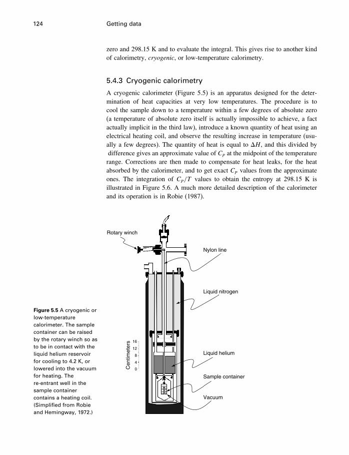
124 Getting data
zero and 298.15 K and to evaluate the integral. This gives rise to another kindof calorimetry, cryogenic, or low-temperature calorimetry.
5.4.3 Cryogenic calorimetry
A cryogenic calorimeter (Figure 5.5) is an apparatus designed for the deter-mination of heat capacities at very low temperatures. The procedure is tocool the sample down to a temperature within a few degrees of absolute zero(a temperature of absolute zero itself is actually impossible to achieve, a factactually implicit in the third law), introduce a known quantity of heat using anelectrical heating coil, and observe the resulting increase in temperature (usu-ally a few degrees). The quantity of heat is equal to �H , and this divided bydifference gives an approximate value of CP at the midpoint of the temperaturerange. Corrections are then made to compensate for heat leaks, for the heatabsorbed by the calorimeter, and to get exact CP values from the approximateones. The integration of CP/T values to obtain the entropy at 298.15 K isillustrated in Figure 5.6. A much more detailed description of the calorimeterand its operation is in Robie (1987).
Figure 5.5 A cryogenic orlow-temperaturecalorimeter. The samplecontainer can be raisedby the rotary winch so asto be in contact with theliquid helium reservoirfor cooling to 4.2 K, orlowered into the vacuumfor heating. There-entrant well in thesample containercontains a heating coil.(Simplified from Robieand Hemingway, 1972.)
Nylon line
Rotary winch
Liquid nitrogen
Liquid helium
Sample container
Vacuum
Cen
timet
ers 16
12
8
4
0
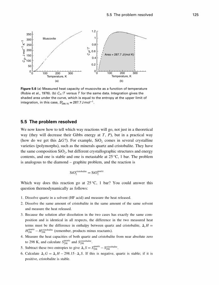
5.5 The problem resolved 125
Muscovite
Temperature, K Temperature, K
Area = 287.7 J/(mol K)
0 0100 100200 200300 300
(b)(a)
0 0
50
100
150
200
250
300
350
Cp
, J m
ol–1
K–1
0.2
0.4
0.6
0.8
1
1.2
CP
/ TFigure 5.6 (a) Measured heat capacity of muscovite as a function of temperature(Robie et al., 1976). (b) CP /T versus T for the same data. Integration gives theshaded area under the curve, which is equal to the entropy at the upper limit ofintegration, in this case, S�
298�15 = 287�7 J mol−1.
5.5 The problem resolved
We now know how to tell which way reactions will go, not just in a theoreticalway (they will decrease their Gibbs energy at T , P), but in a practical way(how do we get this �G?). For example, SiO2 comes in several crystallinevarieties (polymorphs), such as the minerals quartz and cristobalite. They havethe same composition SiO2, but different crystallographic structures and energycontents, and one is stable and one is metastable at 25 �C, 1 bar. The problemis analogous to the diamond – graphite problem, and the reaction is
SiOcristobalite2 = SiOquartz
2
Which way does this reaction go at 25 �C, 1 bar? You could answer thisquestion thermodynamically as follows:
1. Dissolve quartz in a solvent (HF acid) and measure the heat released.
2. Dissolve the same amount of cristobalite in the same amount of the same solvent
and measure the heat released.
3. Because the solution after dissolution in the two cases has exactly the same com-
position and is identical in all respects, the difference in the two measured heat
terms must be the difference in enthalpy between quartz and cristobalite, �rH =H
quartz298 −Hcristobalite
298 (remember, products minus reactants).
4. Measure the heat capacities of both quartz and cristobalite from near absolute zero
to 298 K, and calculate Squartz298 and Scristobalite298 .
5. Subtract these two entropies to give �rS = Squartz298 −Scristobalite298 .
6. Calculate �rG = �rH − 298�15 ·�rS. If this is negative, quartz is stable; if it is
positive, cristobalite is stable.
126 Getting data
Sulfur and the third law of thermodynamics
The problem is which of the two crystalline forms of sulfur is more stable? This
is equivalent to asking what is �G� for the reaction
S�rhomb�= S�mono�
This is the example used by Lewis and Randall (1923) to illustrate calculation of
Gibbs energies.
Equilibrium method The only data available are the heat capacities of rhom-
bic and monoclinic sulfur from 0 to 100 �C, and the enthalpy of transition betweenthe two forms at 0 �C.
�C�P =−0�50T +0�0025T 2 calmol−1 K−1
�transH� = 77�0 calmol−1
General integration of Equation (3.31) gives an integration constant on each side,
which can be combined into one, and at 273.15K �H� is 77.0 calmol−1, allowing
calculation of the constant. General integration of
d�S�
dT= �C�
P
T
results in another integration constant, and combining these expressions with
�G= �H−T�S gives
�G� = 120�3+0�50T lnT −0�00125T 2+ IT
The crucial point is that the equilibrium temperature at which �G� = 0 is known
to be 95 �C, allowing I to be calculated. Thus �G� at 25 �C is calculated to be
17.5 calmol−1.
The third law method Modern data from the JANAF tables (Chase, 1998)
give
Srhomb = 32�056 Jmol−1
Smono = 33�028 Jmol−1
�transH� = 0�360kJmol−1
(continued)
5.5 The problem resolved 127
Then
�G� = �H� −T�S�
= 360−298�15�33�028−32�056�
= 70�2 Jmol−1
= 16�8calmol−1
Putting �G� = 0 the equilibrium temperature is predicted to be 97.2 �C.
You are no doubt quite sure that you don’t have to do this incredible amountof work to answer such a simple question; there must be an easier way. Well,there is, but only because other people have already done this incredible amountof work, and lots more like it. In other words, you can look up the data intables. However, you do not look up heats of solution.
The trick we have just used to get the difference in enthalpy between twominerals (that is, to dissolve them both and subtract the heats of solution) isa very useful way of determining heats of reaction, because many reactionsproceed very slowly, or not at all, and so you cannot measure the heat ofreaction directly in a calorimeter. You cannot measure the heat of reaction ascristobalite changes directly into quartz at 25 �C, because it never does – it isa truly metastable form of SiO2. However, most minerals will dissolve fairlyrapidly in some kind of solvent, providing an indirect means of getting theirenthalpy differences.
To have tables of data that enable you to calculate �rH for any reaction,it would seem that all you need to do is tabulate heats of solution. But if youthink about this for a minute or so, you find that although fine in theory, thiswill not work well in practice. For one thing, you would need to tabulate heatsof solution for all combinations of substances that might be of interest. Thatis, the heats of solution of gibbsite, corundum, and water separately are notenough – you need the heat of solution of corundum + water in a 1:1 ratio. Butfor other reactions, you would need corundum + water in other proportions.Then you would need to be sure that the solution compositions were identi-cal, and given the variety and concentrations of solvents used, your databasewould soon become very large and unmanageable. This problem is resolved,of course, by using “formation from the elements” properties, as discussed inChapter 3. This enables us to tabulate a single number for each property for eachcompound, and makes calculation of reaction deltas easy, at least for standardconditions.
128 Getting data
5.5.1 Gypsum – anhydrite example
The change in enthalpy for any reaction between compounds for which thereare formation-from-the-element data is given by a simple algebraic addition ofthese �fH
� terms, because in balanced reactions, the elements always cancelout. To take another example, consider reaction (3.20) again
CaSO4�s� (anhydrite)+2H2O�l�= CaSO4 ·2H2O�s� (gypsum) (5.11)
Both gypsum and anhydrite occur at the Earth’s surface, and it is not alwaysclear which is the stable phase. To determine the enthalpy change in thisreaction, we consider the reactions in which each phase in the reaction isformed from its elements:
Ca�s�+S�s�+2O2�g�= CaSO4�s�� �fH�anhydrite
=−1434�11kJmol−1
H2�g�+ 12O2�g�= H2O�l�� �fH
�water
=−285�830kJmol−1
Ca�s�+S�s�+3O2�g�+2H2�g�= CaSO4 ·2H2O�s�� �fH�gypsum
=−2022�63kJmol−1
So for reaction (5.11) we have
�rH� = �fH
�gypsum
−�fH�anhydrite
−2�fH�water
=−2022�63− �−1434�11�−2 �−285�830�
=−16�86kJmol−1
from which we see that the reaction between anhydrite and water to formgypsum is exothermic; that is, 16.86 kJ of heat would be released for everymole of anhydrite reacted.
As mentioned in Chapter 3, it is important to realize that this heat of reaction,�rH
�, is equal to the difference in the absolute enthalpies of the reactants andproducts – the enthalpies of the elements have nothing to do with it, becausethey all cancel out. Thus
�rH� = �fH
�gypsum
−�fH�anhydrite
−2�fH�water
=H�CaSO4 ·2H2O
−H�Ca −H�
S −2H�H2
−3H�O2
− �H�CaSO4
−H�Ca −H�
S −2H�O2�
−2�H�H2O
−H�H2
− 12H
�O2�
=H�CaSO4 ·2H2O
−H�CaSO4
−2H�H2O
=−16�86kJmol−1
(5.12)
If you look carefully, you’ll see that all the H� terms for the elements cancelout. But if you think before you look, you’ll realize that they must cancel out if
5.5 The problem resolved 129
the reaction is balanced. Otherwise there is a mistake somewhere. Despite manystatements to the contrary, the absolute enthalpies of the elements (H�
Ca�H�O2�
etc.) are not assumed to be zero. There is no need to do so, because they allcancel out in balanced reactions.4
As you might expect, all the hard work of cryogenic calorimetry has alreadybeen done too, for most common substances, and the results are obtainable intables and compilations of data. From Appendix B, we find that
S�CaSO4(anhydrite)= 106�7 Jmol−1 K−1
S�CaSO4 ·2H2O(gypsum)= 194�1 Jmol−1 K−1
S�H2O(water)= 69�91 Jmol−1 K−1
and the entropy of reaction for (5.11) is
�rS� = S�gypsum −S�anhydrite−2S�water
= 194�1−106�7−2�69�91�
=−52�42 Jmol−1 K−1
So is gypsum or anhydrite stable?Now that we have numerical values for both �rH
� and �rS� for reaction (5.11),it is a simple matter to calculate �rG
� to see which way the reaction goes. Ournumber for enthalpy is in kJ and that for entropy is in J, so we must convertone of them to be consistent. Converting kJ to J, we have
�rG� = �rH� −T �rS�
= −16860−298�15�−52�42�
=−1231 Jmol−1
which is negative; therefore, gypsum is more stable than anhydrite in thepresence of water at Earth surface conditions. We repeat that what we havefound is that the assemblage of anhydrite plus water is metastable with respectto gypsum at 25 �C, 1 bar.5 Anhydrite by itself is not metastable, as there is noother form of CaSO4 that has a lower energy.
4 In the derivation of the enthalpies and Gibbs energies of aqueous ions, the assumption that theproperties of the elements are zero is convenient, but even there it is not necessary(Chapter 15).
5 Actually, we are not really sure whether it is metastable or unstable. The reaction betweenwater and anhydrite to form gypsum is probably very, very slow at 25 �C, but much faster atslightly higher temperatures. This is an example of the discussion in §4.9.1. Metastable is arather fuzzy concept in geology, but crystal clear in thermodynamics.
130 Getting data
Gibbs energy From tablesAlthough we must do the calorimetry experiments in order to calculate freeenergy differences, there is usually no need to use �rH
� and �rS� values
from tables to calculate �rG�. Values of �fG
� for most compounds have beencalculated and are also to be found in the same tables of data, and so we can usethese values directly, instead of going through the �rH
� −T �rS� calculation.For example, �fG
� for anhydrite can be calculated from
�fG�CaSO4
= �fH�CaSO4
−T �fS�CaSO4
where �fS�CaSO4
is
�fS�CaSO4
= S�CaSO4−S�Ca −S�S−2S�O2
Don’t forget that absolute entropies are obtainable for the elements just as wellas for compounds, and these numbers are available in tables of data, such asAppendix B. These numbers are
Substance S�� Jmol−1 K−1
CaSO4�s� 106.7
Ca�s� 41.42
S�s� 31.80
O2�g� 205.138
So
�fS�CaSO4
= 106�7−41�42−31�80−2×205�138
=−376�796 Jmol−1 K−1
Therefore, the Gibbs energy of formation of anhydrite is
�fG�CaSO4
= �fH�CaSO4
−T �fS�CaSO4
=−1434110−298�15�−376�796�
=−1321768 Jmol−1
=−1321�77kJmol−1
which is the number for �fG� in Appendix B (−1321�79 kJmol−1), within the
limits of accuracy of the data.
5.5 The problem resolved 131
The calculation for determining whether gypsum or anhydrite is stable istherefore a little easier – we just look up the �fG
� numbers instead of both the�fH
� and S� numbers. Thus
�rG� = �fG
�CaSO4 ·2H2O
−�fG�CaSO4
−2�fG�H2O
=−1797280− �−1321790�−2�−237129�
=−1232 Jmol−1 (5.13)
which is what we got before (−1231 Jmol−1), within the limits of accuracy ofthe tabulated data.
Again, although we use the Gibbs energies of formation, the G values forthe elements all cancel out, and what we calculate is the difference betweenthe absolute Gibbs energies of the compounds in the reaction. Free energy andenthalpy are similar in this respect.
5.5.2 An aqueous organic example
To emphasize that our model is just as useful for organic or biochemicalprocesses as for mineralogical ones, let’s take another look at the reactioninvolving amino acids we considered in §2.6.1. Equations (2.3) and (2.5) are, torepeat,
C8H16N2O3�aq�+H2O�l�=C6H13NO2�aq�+C2H5NO2�aq� (5.14)
C6H13NO2�aq�+C2H5NO2�aq�=2H2�g�+2NH3�g�+4H2O�l�+8Cgraphite (5.15)
From the tables in Appendix C, we find the following properties:
Substance Formulas �fG�� Jmol−1
leucine C6H13NO2�aq� −343088
glycine C2H5NO2�aq� −370778
leucylglycine C8H16N2O3�aq� −462834
hydrogen H2�g� 0
ammonia NH3�g� −16450
water H2O�l� −237129
graphite C�s� 0
Therefore for reaction (5.14),
�rG� = �fG
�leucine
+�fG�glycine
−�fG�leucylglycine
−�fG�water
=−343088−370778− �−462834�− �−237129�
=−13903 Jmol−1
132 Getting data
and for reaction (5.15)
�rG� = 2�fG
�H2�g�
+2�fG�NH3�g�
+4�fG�H2O�l �
+8�fG�C�s�
−�fG�leucine
−�fG�glycine
= 2 �0�+2 �−16450�+4 �−237129�+8 �0�
− �−343088�− �−370778�
=−267550 Jmol−1
Thus we see that, as illustrated in Figure 2.8, both reactions have a negative“chemical energy,” or �rG
�. However, to say any more about these reactions,we must emphasize a factor we have not yet mentioned, and which we cannotdevelop fully until Chapter 9 (§9.9).
The problem with solutionsIt matters not a bit whether the substances we consider are organic or inorganic,stable or metastable, as long as we have data for them. But it matters a greatdeal whether they are pure substances (such as gypsum, quartz, diamond,liquid water, etc.) or are dissolved in some solvent, as with all substancesdesignated �aq� in the tables. The problem is that the Gibbs energy (and allother properties) of a pure substance is a fixed and known quantity, but theGibbs energy of a substance in solution depends on its concentration. Thetabulated values of �fG
� for �aq� substances are for one particular standardconcentration. Therefore, although we have calculated a negative �rG
� forour two reactions above, they both involve at least some dissolved substancesand, therefore, the conclusion that the reactions should proceed spontaneouslyapplies only when all the �aq� substances have the standard concentrations.We look more carefully at these problems in Chapters 7, 8, and 9.
Enzymes as catalystsOne more thing to note about chemical reactions is that living organisms haveevolved mechanisms involving enzymes that overcome the energy barriersbetween reactants and products for reactions required by the organism. Suchreactions, therefore, proceed easily and quickly, whereas in the inorganic world,diamond persists forever in its metastable state. No organism needs to changediamond to graphite, so no enzymes exist for this reaction. Living organismsalso have mechanisms that drive some reactions “uphill,” or against the Gibbsenergy gradient. Thus peptide bonds are formed in organisms, as well as broken.The energy required to do this is obtained ultimately from the sun, but the
5.6 Data at higher temperatures 133
exact mechanisms are complex. The study of such reactions forms a large partof the science of biochemistry.
5.6 Data at higher temperatures
Everything we have discussed so far is about determining data for “standardconditions,” which usually means pure phases at 25 �C, 1 bar, although wewill see later that it can mean something else. But as geologists we often dealwith reactions at metamorphic and igneous temperatures of many hundreds ofdegrees. Specialized calorimeters can be used up to a few hundred degrees, butthe experimental difficulties become great.
Obviously other methods are needed. As usual, there are several, but wewill mention just two.
5.6.1 Drop calorimetry
The amount of heat required to raise the temperature of a mole of substancefrom Tr to T at constant pressure is simply HT−HTr (or H�
T−H�Trfor a standard
reference substance); again, a difference between two unknown quantities. Thisquantity is conveniently determined by cooling the substance from T to Tr andmeasuring the amount of heat given up by the substance during this process.6
To do this, a calorimeter is placed directly under a furnace and the sample isdropped from the furnace where it has temperature T1, into the calorimeter,where it gives up its heat and achieves temperature T2 (Figure 5.7). The amountof heat given up by the sample is determined by using this heat to melt aworking substance in the calorimeter (either H2O or diphenyl ether �C6H5�2O),and measuring the volume change of this substance by the displacement ofmercury. The relationship between the volume change and the �H of thesolid→liquid phase transition (T2 in the calorimeter is 273.15K for H2O;303.03K for diphenyl ether) is accurately known, so this amount of heat equalsHT1 −HT2 . Small corrections are then applied using heat capacities to adjust this�H to HT −HTr , where Tr is invariably 298.15K. More details of the methodare given by Robie (1987). Experimental results for muscovite are shown inFigure 5.8.
Values of HT −HTr can be combined to give �fH� for substances at high
temperatures. Thus for any substance
�fH�T= �fH
�Tr+�f �H
�T −H�
Tr� (5.16)
6 As a matter of fact, drop calorimetry has been largely superseded by differential scanningcalorimetry (DSC) (§5.6.2), but I include a description here because it illustrates theacquisition of high temperature enthalpies and heat capacities more intuitively than does DSC,and because much of presently used data were obtained by this method.
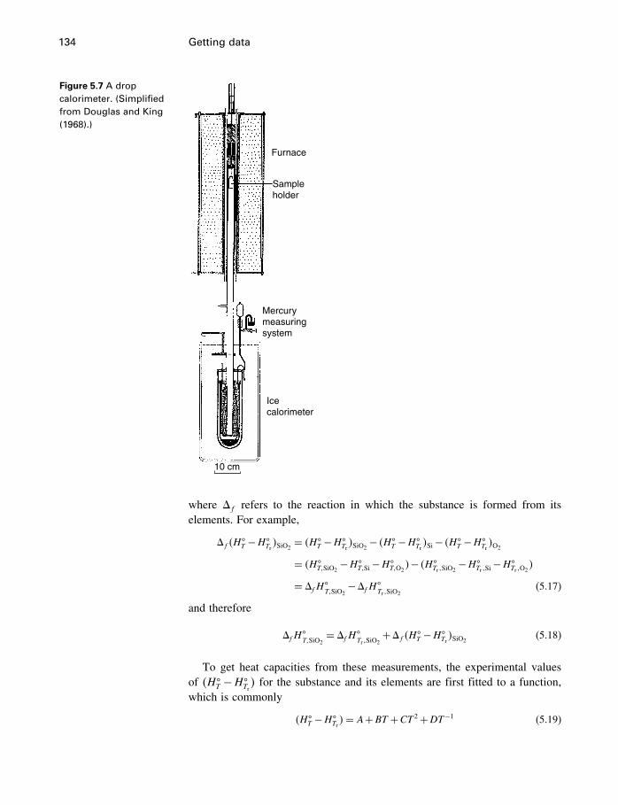
134 Getting data
Figure 5.7 A dropcalorimeter. (Simplifiedfrom Douglas and King(1968).)
Furnace
Mercurymeasuringsystem
Icecalorimeter
10 cm
Sampleholder
where �f refers to the reaction in which the substance is formed from itselements. For example,
�f �H�T −H�
Tr�SiO2
= �H�T −H�
Tr�SiO2
− �H�T −H�
Tr�Si− �H�
T −H�Tr�O2
= �H�T�SiO2
−H�T�Si−H�
T�O2�− �H�
Tr �SiO2−H�
Tr �Si−H�
Tr �O2�
= �fH�T�SiO2
−�fH�Tr �SiO2
(5.17)
and therefore
�fH�T�SiO2
= �fH�Tr �SiO2
+�f �H�T −H�
Tr�SiO2
(5.18)
To get heat capacities from these measurements, the experimental valuesof �H�
T −H�Tr� for the substance and its elements are first fitted to a function,
which is commonly
�H�T −H�
Tr�= A+BT +CT 2+DT−1 (5.19)
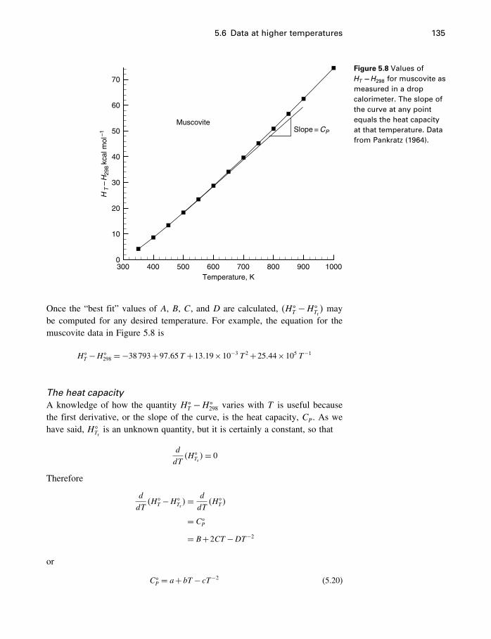
5.6 Data at higher temperatures 135
Temperature, K
HT
–H
298
kcal
mol
–1
300 400 500 600 700 800 900 10000
10
20
30
40
50
60
70
MuscoviteSlope = CP
Figure 5.8 Values ofHT −H298 for muscovite asmeasured in a dropcalorimeter. The slope ofthe curve at any pointequals the heat capacityat that temperature. Datafrom Pankratz (1964).
Once the “best fit” values of A, B, C, and D are calculated, �H�T −H�
Tr� may
be computed for any desired temperature. For example, the equation for themuscovite data in Figure 5.8 is
H�T −H�
298 =−38793+97�65T +13�19×10−3 T 2+25�44×105 T−1
The heat capacityA knowledge of how the quantity H�
T −H�298 varies with T is useful because
the first derivative, or the slope of the curve, is the heat capacity, CP. As wehave said, H�
Tris an unknown quantity, but it is certainly a constant, so that
d
dT�H�
Tr�= 0
Therefore
d
dT�H�
T −H�Tr�= d
dT�H�
T �
= C�P
= B+2CT −DT−2
or
C�P = a+bT − cT−2 (5.20)
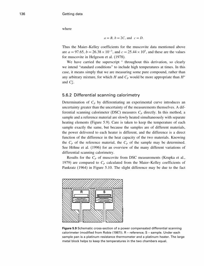
136 Getting data
where
a= B, b = 2C, and c =D�
Thus the Maier–Kelley coefficients for the muscovite data mentioned aboveare a= 97�65, b= 26�38×10−3, and c= 25�44×105, and these are the valuesfor muscovite in Helgeson et al. (1978).
We have carried the superscript � throughout this derivation, so clearlywe intend “standard conditions” to include high temperatures at times. In thiscase, it means simply that we are measuring some pure compound, rather thanany arbitrary mixture, for which H and CP would be more appropriate than H�
and C�P.
5.6.2 Differential scanning calorimetry
Determination of CP by differentiating an experimental curve introduces anuncertainty greater than the uncertainty of the measurements themselves. A dif-ferential scanning calorimeter (DSC) measures CP directly. In this method, asample and a reference material are slowly heated simultaneously with separateheating elements (Figure 5.9). Care is taken to keep the temperature of eachsample exactly the same, but because the samples are of different materials,the power delivered to each heater is different, and the difference is a directfunction of the difference in the heat capacity of the two materials. Knowingthe CP of the reference material, the CP of the sample may be determined.See Höhne et al. (1996) for an overview of the many different variations ofdifferential scanning calorimetry.
Results for the CP of muscovite from DSC measurements (Krupka et al.,1979) are compared to CP calculated from the Maier–Kelley coefficients ofPankratz (1964) in Figure 5.10. The slight difference may be due to the fact
Figure 5.9 Schematic cross-section of a power compensated differential scanningcalorimeter (modified from Robie (1987)). R – reference; S – sample. Under eachsample pan is a platinum resistance thermometer and a platinum heater. The largemetal block helps to keep the temperatures in the two chambers equal.
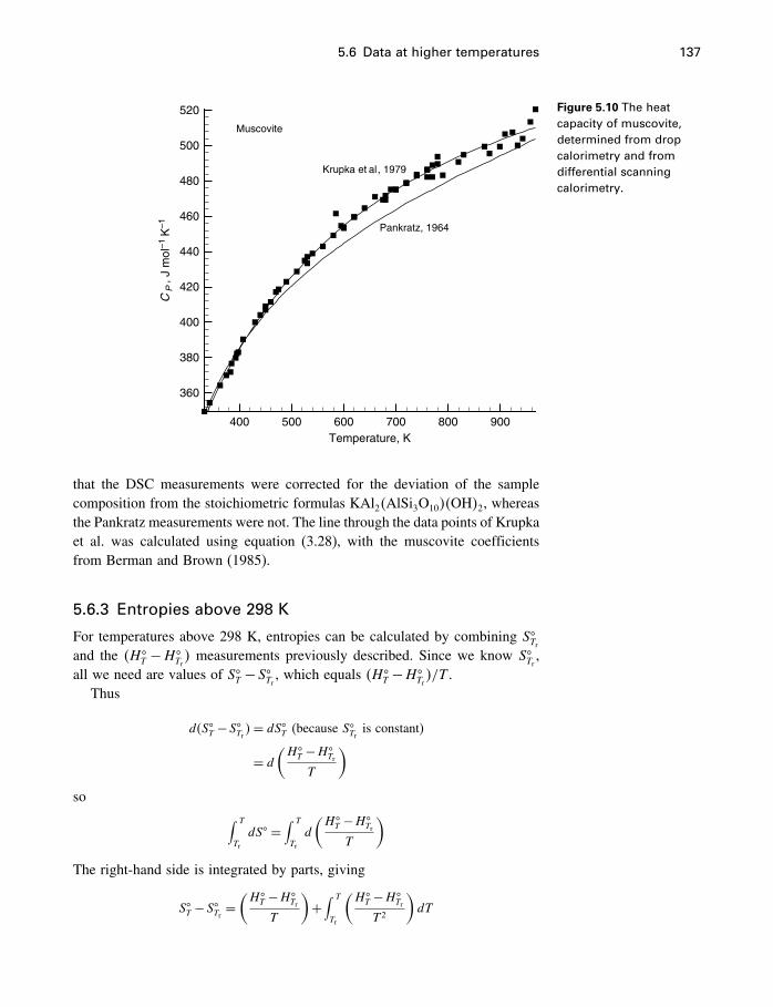
5.6 Data at higher temperatures 137
Temperature, K
CP
, J m
ol–1
K–1
400 500 600 700 800 900
360
380
400
420
440
460
480
500
520
Pankratz, 1964
Krupka et al, 1979
Muscovite
Figure 5.10 The heatcapacity of muscovite,determined from dropcalorimetry and fromdifferential scanningcalorimetry.
that the DSC measurements were corrected for the deviation of the samplecomposition from the stoichiometric formulas KAl2�AlSi3O10��OH�2, whereasthe Pankratz measurements were not. The line through the data points of Krupkaet al. was calculated using equation (3.28), with the muscovite coefficientsfrom Berman and Brown (1985).
5.6.3 Entropies above 298 K
For temperatures above 298 K, entropies can be calculated by combining S�Trand the �H�
T −H�Tr� measurements previously described. Since we know S�Tr ,
all we need are values of S�T −S�Tr , which equals �H�T −H�
Tr�/T .
Thus
d�S�T −S�Tr �= dS�T (because S�Tr is constant)
= d(H�T −H�
Tr
T
)so ∫ T
Tr
dS� =∫ T
Tr
d
(H�T −H�
Tr
T
)The right-hand side is integrated by parts, giving
S�T −S�Tr =(H�T −H�
Tr
T
)+∫ T
Tr
(H�T −H�
Tr
T 2
)dT
138 Getting data
Since �H�T −H�
Tr� and therefore �H�
T −H�Tr�/T 2 is known as a function of T , the
integral can be evaluated, and S�T values calculated for elevated temperatures.As in the case of �H� values, an alternative and usually preferable method isto calculate S�T values, or more likely �rS
� values, at elevated temperatures bymeans of the Maier–Kelley heat capacity coefficients. In other words, since
d
dT�S��= C�
P
T
then
d
dT��rS
��= �rC�P
T
where �rS� refers to the entropy change of a balanced chemical reaction.
Integrating, ∫ T
Tr
d�rS� =
∫ T
Tr
�rC�P
TdT (5.21)
Combining this with the Maier–Kelley equation
�C�P = �a+�bT −�cT−2 (5.22)
we have
�rS�T −�rS�Tr =
∫ T
Tr
(�ra
T+�rb−
�rc
T 3
)dT
or
�rS�T −�rS
�Tr= �ra ln
(T
Tr
)+�rb�T −Tr�+
�rc
2
(1T 2
− 1
Tr2
)(5.23)
In this equation �rS�T refers to the entropy change of any balanced chemical
reaction at temperature T . If the reaction is the formation of a compound fromits elements, �rS
�T becomes �f S
�T .
The apparent entropy of formation can be calculated from
�aS�T = �f S
�Tr+∫ T
Tr
C�P
TdT
where C�P/T refers to the compound only.
5.6.4 Gibbs energies above 298 K
Standard Gibbs energies of formation from the elements at 298 K are computedfrom
�fG�Tr= �fH
�Tr−Tr�fS�Tr (5.24)
5.6 Data at higher temperatures 139
and at higher temperatures from
�fG�T= �fH
�T−T�f S
�T
Using the heat capacity approach, for apparent Gibbs energies at highertemperatures for a compound i
�aG�T�i = �fG
�Tr �i
+∫ T
Tr
��G�i /�T�dT (5.25)
= �fG�Tr �i
+∫ T
Tr
−S�i dT
= �fG�Tr �i
+∫ T
Tr
[−S�Tr �i−
∫ T
Tr
C�P i
TdT
]dT
= �fG�Tr �i
−S�Tr �i�T −Tr�−∫ T
Tr
[∫ T
Tr
C�P i
TdT
]dT
The integration in the last term is performed by parts. That is∫udv= uv−
∫vdu
where
u=∫ T
Tr
C�P i
TdT and v= T
This results in
�aG�T�i = �fG
�Tr �i
−S�Tr �i�T −Tr�+∫ T
Tr
C�P i dT −T
∫ T
Tr
C�P i
TdT (5.26)
which, after substitution of∫ T
Tr
C�PdT = a�T −Tr�+
b
2�T 2−T 2
r �+ c(1T− 1Tr
)(5.27)
and ∫ T
Tr
C�P
TdT = a ln
(T
Tr
)+b�T −Tr�+
c
2
(1T 2
− 1T 2r
)(5.28)
and collection of terms, results in
�aG�T�i
= �fG�Tr �i
−S�Tr �i�T −Tr�
+ai[T −Tr −T ln
(T
Tr
)]+ bi
2
(2TTr −T 2−Tr2
)+ ci
(T 2+T 2
r −2TTr)
2TT 2r
(5.29)
140 Getting data
For a mineral reaction, �rG� is obtained by substituting �rS
�Tr
for S�Tr�iand �ra, �rb, and �rc for ai, bi, and ci, where �ra, etc. are the usualproduct−reactant terms.Thus
�rG�T = �rG
�Tr−�rS
�Tr�T −Tr�
+�ra
[T −Tr −T ln
(T
Tr
)]+ �rb
2
(2TTr −T 2−Tr2
)+ �rc
(T 2+T 2
r −2TTr)
2TT 2r
(5.30)
A special case would be the reaction in which i is formed from its elements,all at T , in which case �rS
�Trbecomes �f S
�Tr�i
, �ra becomes �fai, and so on,and Equation (5.30) then gives �fG
�, the traditional Gibbs energy of formationas a function of T for compound i, but this would perhaps only be of interestto compare with older data compilations which use this quantity.
High temperature muscovite free energiesEquation (5.29) is used to calculate Gibbs energy values in many programs,including supcrt92. To illustrate this consider muscovite again. The requiredinformation is shown in Table 5.1. We have by now seen how all of thesequantities were (or might have been) derived.
Table 5.2 shows the result of plugging the values from Table 5.1 intoEquation (5.29), compared to the values from supcrt92. The values are identicalup to 100 �C, but then begin to deviate. This is because the values fromsupcrt92 are not all at 1 bar. Above 100 �C they are at the pressure of thewater – steam equilibrium. Clearly this pressure difference has an effect on theGibbs energy, to be discussed next.
Table 5.1 Data for muscovite forEquation (5.29), plus the molarvolume.
�fG�Tr
−1336 301 calmol−1
S�Tr 68.8 calmol−1 K−1
a 97.56 calmol−1
b 0.026 38 calmol−1 K−1
c 2 544 000 calmol−1 K2
V 140.7 cm3 mol−1
5.7 Data at higher pressures 141
Table 5.2 The apparent Gibbs energy of formation of muscovite, fromsupcrt92 and from Equation (5.29). Data in calmol−1.
T �C P bars supcrt92 Equation (5.29) Difference P correction = V�P−1�
0.01 1.000 −1334 662 −1334 662 0 0
25 1.000 −1336 301 −1336 301 0 0
50 1.000 −1338 101 −1338 101 0 0
75 1.000 −1340 059 −1340 059 0 0
100 1.013 −1342 171 −1342 171 0 0
125 2.320 −1344 428 −1344 432 4 4
150 4.757 −1346 825 −1346 838 13 13
175 8.918 −1349 357 −1349 383 26 27
200 15.536 −1352 015 −1352 063 48 49
225 25.479 −1354 792 −1354 874 82 82
250 39.736 −1357 680 −1357 811 131 130
275 59.431 −1360 673 −1360 869 196 197
300 85.838 −1363 760 −1364 046 286 285
325 120.458 −1366 935 −1367 337 402 402
350 165.211 −1370 187 −1370 739 552 552
5.7 Data at higher pressures
Fundamentally, to know �G� at any T and P, we need to be able to evaluate
�aG�T�P�i = �fG
�Tr �Pr �i
+∫ T
Tr
��G�i /�T�P=PrdT +
∫ P
Pr
��G�i /�P�T=TdP (5.31)
and there are similar equations for enthalpy and entropy. The integrals inEquation (5.31) take care of the change in G with T and P, respectively, andwe have just seen how the temperature integral is handled in Equation (5.25).The second integral shows that we need to know how G varies with pressureat high temperatures.
In this section we will discuss only the effect of pressure on solid phases,i.e., minerals. The evaluation of the pressure integral is done in quite a differentway for gases, water, and aqueous solutes, and will be treated in later chapters.
5.7.1 Effect of P on Gibbs energy
As shown previously (Equation 4.43), the derivative of G with respect to P isV , i.e.,
��Gi/�P�T = Vi [4.43]
so that to calculate the effect of P on Gi we must know how Vi varies as afunction of P.
142 Getting data
Constant VWhen substance i is a solid phase and thus has relatively small variation of Vwith both P and T (relative that is to liquids and gases), the errors introducedby the assumption that V is not affected by P or T tend to cancel one another,and very little error is introduced by assuming that Vi is a constant at all P�Tvalues. As a result, the assumption of constant V for solids is often adoptedfor minerals, and results in∫ P
Pr
��Gi/�P�TdP =Gi�P−Gi�Pr= Vi�P−1� (5.32)
where Vi is the molar volume of the solid phase in J bar−1, and Pr = 1 bar.Determination of the molar volume can be done experimentally, but is morecommonly calculated from X-ray determination of the mineral structure. Thisterm Vi�P− 1� is then added to the right side of Equation (5.29) to evaluate�aG
� at high pressures as well as high temperatures, giving
�aG�T�i
= �fG�Tr �i
−S�Tr �i�T −Tr�ai[T −Tr −T ln
(T
Tr
)]
+ bi2
(2TTr −T 2−Tr2
)+ ci (T 2+T 2r −2TTr
)2TT 2
r
+Vi�P−1� (5.33)
An example of this for muscovite is shown in Table 5.2.If we are dealing with a mineral reaction (that is, a reaction involving
only solid phases for which (4.43) is valid) instead of a pure compound, wesubstitute �rS
�Trfor S�Tr�i and �ra, �rb, and �rc for ai, bi, and ci, where �ra,
etc. are the usual product–reactant terms, just as we did in Equation (5.30).Equation (5.33) then becomes
�rG�T�i
= �rG�Tr �i
−�rS�Tr �i�T −Tr�+�rai
[T −Tr −T ln
(T
Tr
)]
+ �rbi2
(2TTr −T 2−Tr2
)+ �rci(T 2+T 2
r −2TTr)
2TT 2r
+�rVi�P−1� (5.34)
Variable VAlternatively, some attempt at modeling the temperature and pressure effectson mineral volumes can be attempted (see Helgeson et al., 1978, and Berman,1988 for lengthy discussions of this topic). The only attempt at this to findits way into a widely used database is that of Berman (1988). Berman fit theavailable data for rock-forming minerals to the expression
VP�TVPr �Tr
= 1+v1�P−Pr�+v2�P−Pr�2+v3�T −Tr�+v4�T −Tr�2 (5.35)
where v1 – v4 are fit parameters, Pr = 1 bar, and Tr = 298�15K. The equation hasno theoretical basis, and Berman cautions against its use at conditions beyond
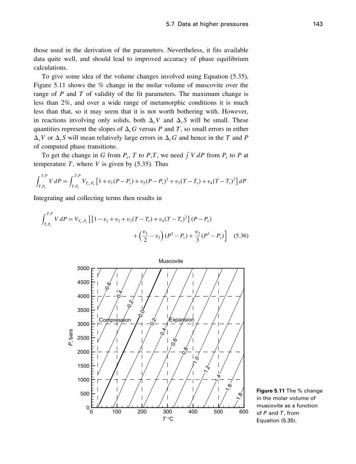
5.7 Data at higher pressures 143
those used in the derivation of the parameters. Nevertheless, it fits availabledata quite well, and should lead to improved accuracy of phase equilibriumcalculations.
To give some idea of the volume changes involved using Equation (5.35),Figure 5.11 shows the % change in the molar volume of muscovite over therange of P and T of validity of the fit parameters. The maximum change isless than 2%, and over a wide range of metamorphic conditions it is muchless than that, so it may seem that it is not worth bothering with. However,in reactions involving only solids, both �rV and �rS will be small. Thesequantities represent the slopes of �rG versus P and T , so small errors in either�rV or �rS will mean relatively large errors in �rG and hence in the T and Pof computed phase transitions.
To get the change in G from Pr , T to P,T , we need∫V dP from Pr to P at
temperature T , where V is given by (5.35). Thus∫ T�P
T�Pr
V dP =∫ T�P
T�Pr
VTr �Pr[1+v1�P−Pr�+v2�P−Pr�
2+v3�T −Tr�+v4�T −Tr�2]dP
Integrating and collecting terms then results in
∫ T�P
T�Pr
V dP = VTr �Pr[{1−v1+v2+v3�T −Tr�+v4�T −Tr�2
}�P−Pr�
+(v12−v2
)�P2−Pr�+
v23�P3−Pr�
](5.36)
T °C
P, b
ars
0 100 200 300 400 500 6000
500
1000
1500
2000
2500
3000
3500
4000
4500
5000Muscovite
Compression Expansion
–0.6
–0.4
–0.2
0.0
0.2
0.4
0.6
0.8
1.0
1.2
1.4
1.6
1.8
Figure 5.11 The % changein the molar volume ofmuscovite as a functionof P and T , fromEquation (5.35).
144 Getting data
The right side of Equation (5.36) could be substituted for Vi�P − 1� inEquation (5.33). Realistically, however, it should probably be used only withthe Berman (1988) database of mineral properties, as it was derived using thisformula.
The Berman–Brown conventionWe mentioned in Chapter 3 the two conventions used to define “apparent”properties, which are used as a form of “formation from the element” prop-erties at temperatures above 298.15K. The Benson–Helgeson convention wasdescribed there. The Berman–Brown convention, although the same for �H�,is different for �G�.
In the Berman–Brown convention, the apparent Gibbs energy, �aG�, is
defined as
�aG�P�T = �aH�
P�T −T ·S�P�T (5.37)
Notice the difference between this equation and Equation (5.1) or Equa-tion (5.24), that is, it uses S�, not �S�. In other words, the entropies of theelements at 298.15K are omitted because they are not needed to define S�.However, it means that while Benson–Helgeson values of �aG
� are the sameas traditional �fG
� values at 298.15K, 1 bar, Berman–Brown values of �aG�
are not.If you integrate Equation (5.31) using both the Berman and Brown (1985)
heat capacity Equation (3.28) and the Berman–Brown convention for �aG�,
you find
�aG�P�T = �fG
�Pr �Tr
−TS�Pr �Tr+k0 ��T −Tr�−T�lnT − lnTr��
+2k1[�T 0�5−Tr0�5�+T�T−0�5−Tr−0�5�
]−k2
[�T−1−Tr−1�− T
2�T−2−Tr−2�
]−k3
[T−2−Tr−2
2− T
3�T−3−Tr−3�
]+VPr �Tr
[(v−12
−v2)�P2−Pr
2�+ v23�P3−Pr
3�
+{1−v−1+v2+v3�T −Tr�+v4�T −Tr�2}�P−Pr�
](5.38)
which is the equivalent of supcrt92’s Equation (5.33). The numbers for indi-vidual minerals these two equations produce are quite different, but for balancedreactions they are very nearly the same.
5.8 Other methods 145
5.7.2 Effect of P on enthalpy and entropy
For most geochemical modeling purposes, only the pressure effect on G isrequired. The effect of pressure on S is7(
�S
�P
)T
=−(�V
�T
)P
(5.39)
showing that the effect of pressure on entropy can be obtained by measuringthe effect of temperature on volume (or density), which is usually a muchsimpler task. Fairly simple manipulations then show the effect of pressure onenthalpy to be (
�H
�P
)T
= V −T(�V
�T
)P
(5.40)
Therefore the effect of pressure on H and S using the constant molar volumeassumption (��V/�T�P = 0) is particularly simple. Equation (5.39) shows thatthere is no effect on S, and integration of Equation (5.40) with ��V/�T�P = 0shows that the pressure effect on H is the same as that on G, that is, V�P−1�.
Equations (5.39) and (5.40) result in particularly simple expressions for anideal gas, which are often useful. Substituting RT/P for V in Equation (5.39)leads to
�S = SP2 −SP1= R ln
P2
P1(5.41)
and making the same substitution in (5.40) results in
�H =HP2 −HP2= 0 (5.42)
These results should make intuitive sense. Changing the pressure on an idealgas does not change the fact that there are no interparticle forces, so thereshould be no effect of pressure on energy terms. However, it does change theordering or arrangement of the particles, and hence the entropy.
5.8 Other methods
Up to here in this chapter we have discussed getting data only for solid phases.We have seen that the goal is to determine �aG
� over a wide range of T andP (and that �aG
�= �fG� at 25 �C, 1 bar for one widely used convention, but
7 This equation is obtained by applying the reciprocity relation (Equation C.10) toEquation (4.40).
146 Getting data
not for another). Doing this requires integration of Equation (5.31), which inturn requires that we know how V and CP vary with T and P. For solids, V iseither considered a constant, or its slight variation can be estimated, and CP ismeasured directly (§5.6.2) or indirectly (§5.6.1) by calorimetry.
For gases and liquids the fundamentals are the same (we still must inte-grate (5.31)), but methods are quite different because V is far from constant.For dissolved substances, more difficulties arise because solution propertiesvary with the concentration of the solute, and for electrolytes, there is alsoa variable degree of association of the charged particles. We will mentiona few experimental methods here, but we cannot discuss the data obtaineduntil we learn more about how we deal with the properties of dissolvedsubstances.
5.8.1 Density measurement
The vibrating tube densitometer is an instrument designed to precisely measureliquid or gas density. A tube or spool is vibrated mechanically at its naturalfrequency and sensors measure the frequency of that vibration. The measuredfrequency will decrease as density increases, and can be calculated after cal-ibrating the instrument with fluids of known density. Other density relatedvariables such as specific gravity, molecular weight, and concentration mayalso be calculated. It is now very widely used in industry as well as scientificlaboratories. See, e.g., Majer et al. (1991).
A more direct method is provided by a dilatometer, basically a pressurevessel connected to a mercury reservoir and a glass capillary column. Changesin the height of the mercury in the column are directly related to the change indensity of the fluid in the pressure vessel. The apparatus is calibrated using purewater, with its known volumetric properties. Of course, no brief descriptioncan give any idea of the multitude of details of operation and correction factorsthat go into making precise measurements.
5.8.2 Calorimetry
Calorimetry of liquids and solutes has been revolutionized in recent yearsby the combination of the differential scanning technique, in which somedifference between a sample and a standard is observed, with the continuousflow of fluids through the calorimeter. Instead of having two mineral samples(§5.6.2), two columns or tubes are used, through which a reference solutionand a sample solution flow at a controlled rate (Figure 5.12). As before, thedifference in the power required to keep the columns at the same temperatureis directly related to the difference in the heat capacities of the two fluids.See Wood (1989) for a history of the development of these methods and theiradvantages.
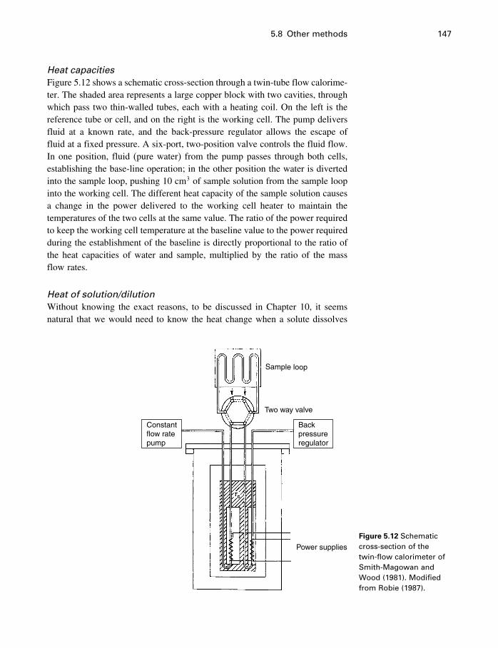
5.8 Other methods 147
Heat capacitiesFigure 5.12 shows a schematic cross-section through a twin-tube flow calorime-ter. The shaded area represents a large copper block with two cavities, throughwhich pass two thin-walled tubes, each with a heating coil. On the left is thereference tube or cell, and on the right is the working cell. The pump deliversfluid at a known rate, and the back-pressure regulator allows the escape offluid at a fixed pressure. A six-port, two-position valve controls the fluid flow.In one position, fluid (pure water) from the pump passes through both cells,establishing the base-line operation; in the other position the water is divertedinto the sample loop, pushing 10 cm3 of sample solution from the sample loopinto the working cell. The different heat capacity of the sample solution causesa change in the power delivered to the working cell heater to maintain thetemperatures of the two cells at the same value. The ratio of the power requiredto keep the working cell temperature at the baseline value to the power requiredduring the establishment of the baseline is directly proportional to the ratio ofthe heat capacities of water and sample, multiplied by the ratio of the massflow rates.
Heat of solution/dilutionWithout knowing the exact reasons, to be discussed in Chapter 10, it seemsnatural that we would need to know the heat change when a solute dissolves
Sample loop
Two way valve
Power supplies
Constantflow ratepump
Backpressureregulator
Figure 5.12 Schematiccross-section of thetwin-flow calorimeter ofSmith-Magowan andWood (1981). Modifiedfrom Robie (1987).
148 Getting data
into a fluid, such as NaCl dissolving in water, i.e., calorimetric heats of solution,either solid into liquid, or liquid into liquid, i.e., mixing of liquid solutions.
A practical consideration in conducting this kind of heat of solution mea-surements is that it is frequently much simpler and more accurate to measureheat flows associated with diluting solutions, rather than with making themmore concentrated. Dissolving NaCl in a concentrated solution of NaCl inwater is a rather slow process, so that the heat is absorbed over a long period oftime, and it is difficult to know when the process is complete. Adding water toa concentrated NaCl solution is on the other hand accomplished fairly quicklyand the same information can be deduced from these dilution measurementsas from “solution” measurements. Of course, what is “dilution” and what is“solution” is to some degree quite arbitrary – a “heat of dilution” on addingwater to NaCl solutions could be considered a “heat of solution” of water in thesystem NaCl–H2O. Normally, however, water is considered the solvent, andadding water is called dilution. Heat of dilution measurements have also bene-fited from the twin-tube differential method. One such instrument is describedby Busey et al. (1984).
5.8.3 Conductance measurements
Electrolyte solutions are those in which the solute (e.g., NaCl) dissociates intocharged particles called ions (e.g., Na+ and Cl−). Naturally, such solutionsare much better conductors of electricity than is the solvent alone (normallywater), and the conductivity of the solution will depend on the extent to whichthe dissociation takes place. That is, if only some of the NaCl dissociatesinto Na+ and Cl−, the solution will be less conducting than if all of it does.Measurement of conductivity is therefore a means of determining the degreeof dissociation of solutes. Significant improvements in the speed and accuracyof conductance measurements has been achieved by using a flow-through cell(Zimmerman et al. 1995).
5.8.4 Isopiestic measurements
Isopiestic means, roughly, equal pressures. In Figure 5.13 a number of con-tainers contain solutions of various concentrations of a salt A, enclosed in asealed, evacuated chamber. One of the containers contains a standard solutionof a salt B, for which the properties are accurately known. As the solutionsall have different vapor pressures, water will slowly evaporate from some andcondense in others until all containers have exactly the same vapor pressure.The properties of the salt and the water in each solution are related in aninteresting way by thermodynamics. Because you know the properties of thestandard solution, and now all solutions have the same water vapor pressure, itis possible to calculate the properties (well, one property anyway) of salt A as
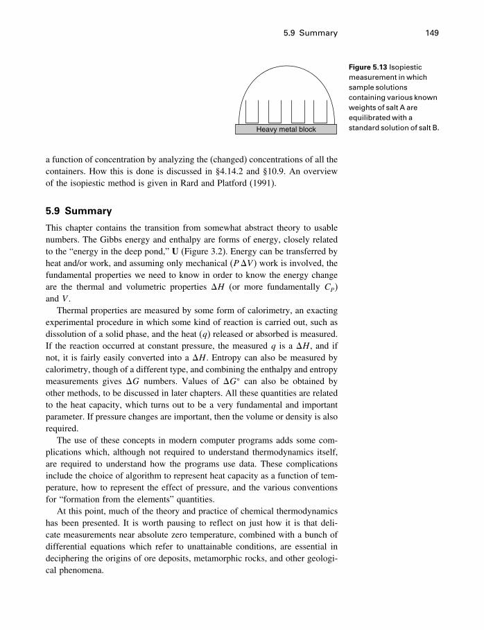
5.9 Summary 149
Heavy metal block
Figure 5.13 Isopiesticmeasurement in whichsample solutionscontaining various knownweights of salt A areequilibrated with astandard solution of salt B.
a function of concentration by analyzing the (changed) concentrations of all thecontainers. How this is done is discussed in §4.14.2 and §10.9. An overviewof the isopiestic method is given in Rard and Platford (1991).
5.9 Summary
This chapter contains the transition from somewhat abstract theory to usablenumbers. The Gibbs energy and enthalpy are forms of energy, closely relatedto the “energy in the deep pond,” U (Figure 3.2). Energy can be transferred byheat and/or work, and assuming only mechanical (P �V ) work is involved, thefundamental properties we need to know in order to know the energy changeare the thermal and volumetric properties �H (or more fundamentally CP)and V .
Thermal properties are measured by some form of calorimetry, an exactingexperimental procedure in which some kind of reaction is carried out, such asdissolution of a solid phase, and the heat (q) released or absorbed is measured.If the reaction occurred at constant pressure, the measured q is a �H , and ifnot, it is fairly easily converted into a �H . Entropy can also be measured bycalorimetry, though of a different type, and combining the enthalpy and entropymeasurements gives �G numbers. Values of �G� can also be obtained byother methods, to be discussed in later chapters. All these quantities are relatedto the heat capacity, which turns out to be a very fundamental and importantparameter. If pressure changes are important, then the volume or density is alsorequired.
The use of these concepts in modern computer programs adds some com-plications which, although not required to understand thermodynamics itself,are required to understand how the programs use data. These complicationsinclude the choice of algorithm to represent heat capacity as a function of tem-perature, how to represent the effect of pressure, and the various conventionsfor “formation from the elements” quantities.
At this point, much of the theory and practice of chemical thermodynamicshas been presented. It is worth pausing to reflect on just how it is that deli-cate measurements near absolute zero temperature, combined with a bunch ofdifferential equations which refer to unattainable conditions, are essential indeciphering the origins of ore deposits, metamorphic rocks, and other geologi-cal phenomena.
6Some simple applications
6.1 Introduction
We now know how to determine in which direction any chemical reaction willproceed at a given temperature and pressure, at least when all the productsand reactants are pure phases. When even one of the products or reactants isa solute, that is, part of a solution, we would be stuck because although wehave had a brief look at how calorimetry can be used with liquids and liquidsolutions, we haven’t yet seen how to use the data obtained. We will startconsidering this problem in the next chapter. Before going on, however, weshould explore some relationships using the concepts we have defined so far,so as to make sure we fully understand them. Naturally, we will only be ableto consider some simple properties of pure phases, and reactions between purephases.
6.2 Some properties of water
Water is an extraordinarily important substance in many ways in Earth pro-cesses, both organic and inorganic. The fact that it is a liquid in the relativelynarrow range of T and P found at the Earth’s surface was of course essentialto the evolution of life. The reason for this, that is, the polar structure of theH2O molecule and its many unusual properties such as hydrogen bonding, isa fascinating subject in physical chemistry. In geochemical thermodynamics,we are concerned only with its macroscopic properties and its role in mineralreactions, both at and near the surface and at depth in the crust, that is, theweathering, metamorphic, and igneous environments.
So what macroscopic properties do we mean? Well, those that are connectedwith heat (q) and work (w), of course. Water is an important agent in thetransport of heat, such as in convecting systems, but this is not really athermodynamic subject. By “connected with heat” I mean things like the heatcapacity, entropy, and enthalpy of water itself, and how changes in theseproperties are of interest. The property connected with work is of course themolar or specific volume.
150
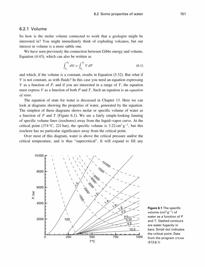
6.2 Some properties of water 151
6.2.1 Volume
So how is the molar volume connected to work that a geologist might beinterested in? You might immediately think of exploding volcanos, but ourinterest in volume is a more subtle one.
We have seen previously the connection between Gibbs energy and volume,Equation (4.43), which can also be written as∫ P2
P1
dG=∫ P2
P1
V dP (6.1)
and which, if the volume is a constant, results in Equation (5.32). But what ifV is not constant, as with fluids? In this case you need an equation expressingV as a function of P, and if you are interested in a range of T , the equationmust express V as a function of both P and T . Such an equation is an equationof state.
The equation of state for water is discussed in Chapter 13. Here we canlook at diagrams showing the properties of water, generated by the equation.The simplest of these diagrams shows molar or specific volume of water asa function of P and T (Figure 6.1). We see a fairly simple-looking fanningof specific volume lines (isochores) away from the liquid–vapor curve. At thecritical point (374 �C, 221 bar), the specific volume is 3.22 cm3 g−1, but thisisochore has no particular significance away from the critical point.
Over most of this diagram, water is above the critical pressure and/or thecritical temperature, and is thus “supercritical”. It will expand to fill any
T °C
P, b
ar
0 250 500 750 1000
2000
4000
6000
8000
10000
1.0
1.2
1.4
1.61.8
2.0
2.53.224.0
10.0
100
10002000
30004000
5000
7500
10000
Figure 6.1 The specificvolume (cm3 g−1) ofwater as a function of Pand T . Dashed contoursare water fugacity inbars. Small dot indicatesthe critical point. Datafrom the program steam(§13.6.1)
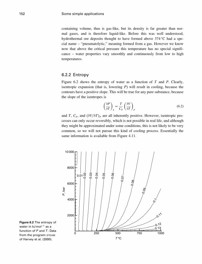
152 Some simple applications
containing volume, thus is gas-like, but its density is far greater than nor-mal gases, and is therefore liquid-like. Before this was well understood,hydrothermal ore deposits thought to have formed above 374 �C had a spe-cial name – “pneumatolytic,” meaning formed from a gas. However we knownow that above the critical pressure this temperature has no special signifi-cance – water properties vary smoothly and continuously from low to hightemperatures.
6.2.2 Entropy
Figure 6.2 shows the entropy of water as a function of T and P. Clearly,isentropic expansion (that is, lowering P) will result in cooling, because thecontours have a positive slope. This will be true for any pure substance, becausethe slope of the isentropes is(
�P
�T
)S
= T
CP
(�V
�T
)P
(6.2)
and T , CP, and ��V/�T�P are all inherently positive. However, isentropic pro-cesses can only occur reversibly, which is not possible in real life, and althoughthey might be approximated under some conditions, this is not likely to be verycommon, so we will not pursue this kind of cooling process. Essentially thesame information is available from Figure 4.11.
Figure 6.2 The entropy ofwater in kJmol−1 as afunction of P and T . Datafrom the program steamof Harvey et al. (2000).
0.01
0.02
0.03
0.04
0.05
0.06
0.07
0.08
0.09
0.1
0.11
0.120.13
T °C
P, b
ar
0 250 500 750 1000
2000
4000
6000
8000
10 000
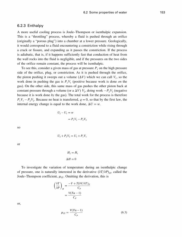
6.2 Some properties of water 153
6.2.3 Enthalpy
A more useful cooling process is Joule–Thompson or isenthalpic expansion.This is a “throttling” process, whereby a fluid is pushed through an orifice(originally a “porous plug”) into a chamber at a lower pressure. Geologically,it would correspond to a fluid encountering a constriction while rising througha crack or fissure, and expanding as it passes the constriction. If the processis adiabatic, that is, if it happens sufficiently fast that conduction of heat fromthe wall rocks into the fluid is negligible, and if the pressures on the two sidesof the orifice remain constant, the process will be isenthalpic.
To see this, consider a given mass of gas at pressure P1 on the high pressureside of the orifice, plug, or constriction. As it is pushed through the orifice,the piston pushing it sweeps out a volume ��V� which we can call V1, so thework done in pushing the gas is P1V1 (positive because work is done on thegas). On the other side, this same mass of gas pushes the other piston back atconstant pressure through a volume (or a �V� V2, doing work −P2V2 (negativebecause it is work done by the gas). The total work for the process is thereforeP1V1−P2V2. Because no heat is transferred, q = 0, so that by the first law, theinternal energy change is equal to the work done, �U = w.
U2−U1 = w= P1V1−P2V2
so
U2+P2V2 = U1+P1V1
or
H2 =H1
�H = 0
To investigate the variation of temperature during an isenthalpic changeof pressure, one is naturally interested in the derivative ��T/�P�H , called theJoule–Thompson coefficient, �JT. Omitting the derivation, this is(
�T
�P
)H
= −V +T��V/�T�PCP
= V�T−1�CP
or,
�JT =V�T−1�CP
(6.3)
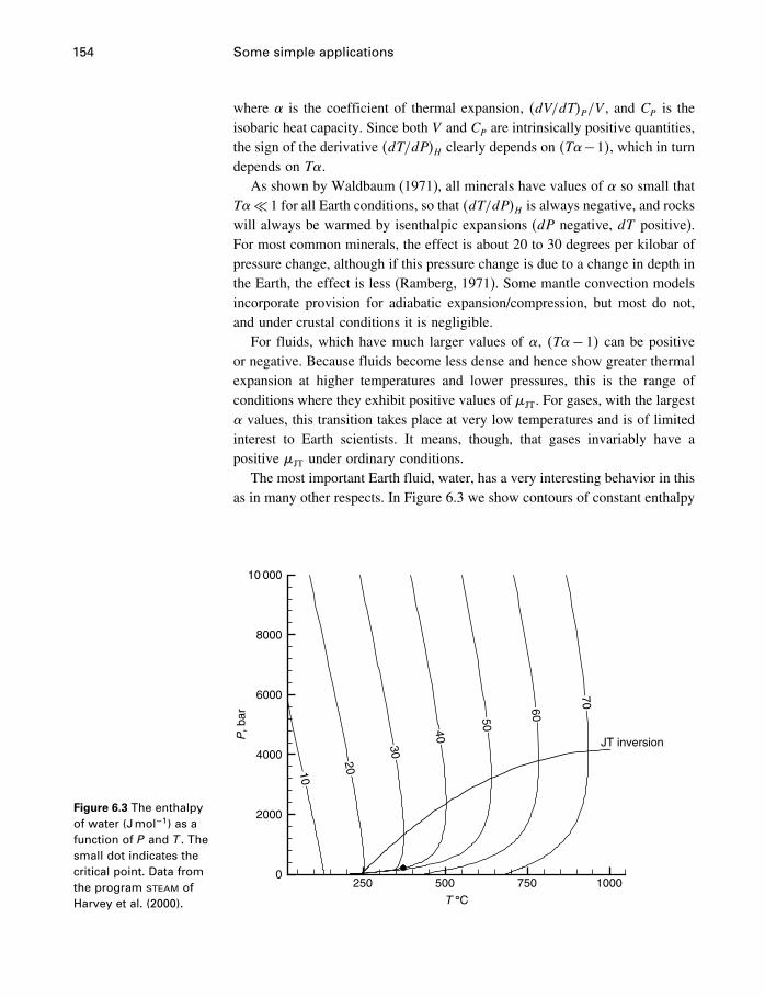
154 Some simple applications
where is the coefficient of thermal expansion, �dV/dT�P/V , and CP is theisobaric heat capacity. Since both V and CP are intrinsically positive quantities,the sign of the derivative �dT/dP�H clearly depends on �T−1�, which in turndepends on T�
As shown by Waldbaum (1971), all minerals have values of so small thatT� 1 for all Earth conditions, so that �dT/dP�H is always negative, and rockswill always be warmed by isenthalpic expansions (dP negative, dT positive).For most common minerals, the effect is about 20 to 30 degrees per kilobar ofpressure change, although if this pressure change is due to a change in depth inthe Earth, the effect is less (Ramberg, 1971). Some mantle convection modelsincorporate provision for adiabatic expansion/compression, but most do not,and under crustal conditions it is negligible.
For fluids, which have much larger values of , �T− 1� can be positiveor negative. Because fluids become less dense and hence show greater thermalexpansion at higher temperatures and lower pressures, this is the range ofconditions where they exhibit positive values of �JT. For gases, with the largest values, this transition takes place at very low temperatures and is of limitedinterest to Earth scientists. It means, though, that gases invariably have apositive �JT under ordinary conditions.
The most important Earth fluid, water, has a very interesting behavior in thisas in many other respects. In Figure 6.3 we show contours of constant enthalpy
Figure 6.3 The enthalpyof water (Jmol−1) as afunction of P and T . Thesmall dot indicates thecritical point. Data fromthe program steam ofHarvey et al. (2000).
10
20
30
40
50
60
70
T °C
P, b
ar
250 500 750 10000
2000
4000
6000
8000
10 000
JT inversion
6.2 Some properties of water 155
Enthalpy, kJ/mol
log
P
20 40 60 80
1.5
2.0
2.5
3.0
3.5
4.0
–0.015
–0.01
00.01
0.05
100
200
300
400
500
600
700
800
2
1
JT inversion curve
Figure 6.4 Isotherms onlogP versus enthalpy inkJmol−1 for water.Dashed contours are theJoule–Thompsoncoefficient, �JT. Thecontour for �JT = 0 is theJoule–Thompsoninversion curve. Datafrom the program steamof Harvey et al. (2000).
of water as a function of P and T .1 Where the contours have a negative slope,water warms on adiabatic expansion and cools if adiabatically compressed.Where they have a positive slope, water cools on adiabatic expansion andwarms if adiabatically compressed, and the two regions are separated by theJoule–Thompson inversion curve. Much the same information is contained inthe enthalpy–pressure diagram (Figure 6.4), where it can be seen that constantenthalpy changes in pressure lead to increases in temperature in one region(arrow 1) and decreases in another (arrow 2).
The effect of dissolved NaCl on the Joule–Thompson coefficient has beencalculated by Wood and Spera (1984), and the effect will be similar for otherelectrolytes. Because the addition of most electrolytes to water results in adecrease in V and in , �JT is smaller, and the net effect is to move theinversion curve to higher temperatures and lower pressures.
Isenthalpic boilingA special case of adiabatic isenthalpic volume change of particular interest togeologists concerned with fluids in the upper levels of the Earth’s crust is thecase where a phase change, especially boiling, occurs along the cooling path ofthe fluid (Figure 6.5). The onset of boiling in a hot aqueous fluid in the crust
1 As in Figures 4.11 and 6.4, these enthalpy numbers use the normal Steam Table convention, inwhich UH2O
= SH2O= 0. Converting Steam Table values to apparent formation from the
elements values (e.g., �aH�) is discussed in Chapter 13, page 388.
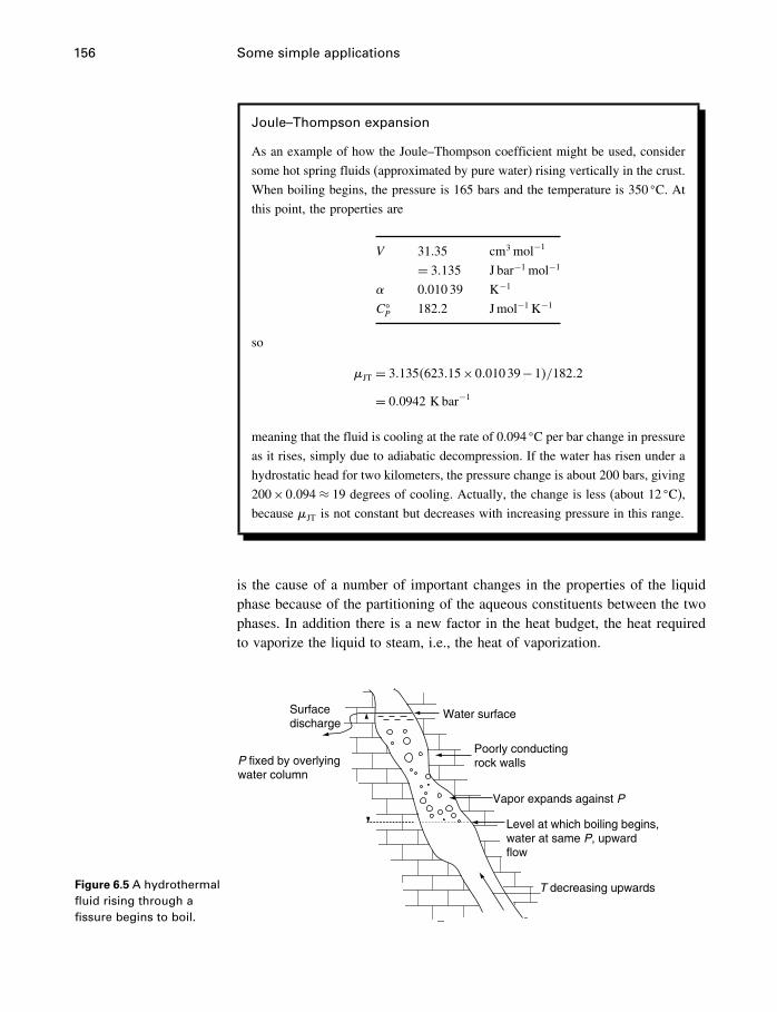
156 Some simple applications
Joule–Thompson expansion
As an example of how the Joule–Thompson coefficient might be used, consider
some hot spring fluids (approximated by pure water) rising vertically in the crust.
When boiling begins, the pressure is 165 bars and the temperature is 350 �C. Atthis point, the properties are
V 31.35 cm3 mol−1
= 3�135 J bar−1 mol−1
0.010 39 K−1
C�P 182.2 Jmol−1 K−1
so
�JT = 3�135�623�15×0�01039−1�/182�2
= 0�0942 K bar−1
meaning that the fluid is cooling at the rate of 0.094 �C per bar change in pressure
as it rises, simply due to adiabatic decompression. If the water has risen under a
hydrostatic head for two kilometers, the pressure change is about 200 bars, giving
200×0�094≈ 19 degrees of cooling. Actually, the change is less (about 12 �C),because �JT is not constant but decreases with increasing pressure in this range.
is the cause of a number of important changes in the properties of the liquidphase because of the partitioning of the aqueous constituents between the twophases. In addition there is a new factor in the heat budget, the heat requiredto vaporize the liquid to steam, i.e., the heat of vaporization.
Figure 6.5 A hydrothermalfluid rising through afissure begins to boil.
Water surface
Poorly conducting rock walls
Vapor expands against P
Level at which boiling begins, water at same P, upward flow
T decreasing upwards
Surfacedischarge
P fixed by overlying water column
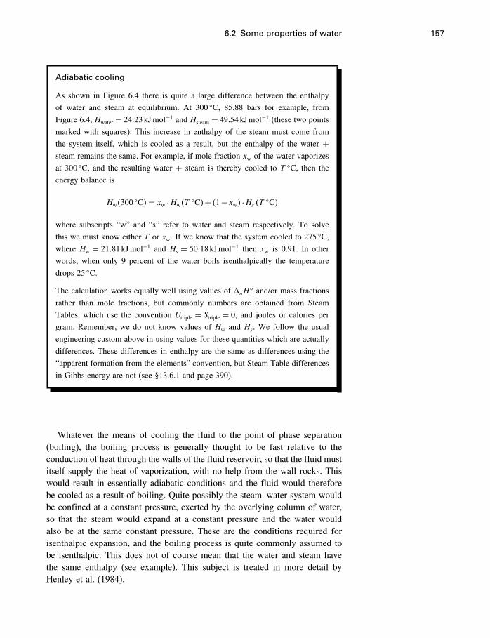
6.2 Some properties of water 157
Adiabatic cooling
As shown in Figure 6.4 there is quite a large difference between the enthalpy
of water and steam at equilibrium. At 300 �C, 85.88 bars for example, from
Figure 6.4, Hwater = 24�23kJmol−1 and Hsteam = 49�54kJmol−1 (these two points
marked with squares). This increase in enthalpy of the steam must come from
the system itself, which is cooled as a result, but the enthalpy of the water +steam remains the same. For example, if mole fraction xw of the water vaporizes
at 300 �C, and the resulting water + steam is thereby cooled to T �C, then the
energy balance is
Hw�300�C�= xw ·Hw�T
�C�+ �1−xw� ·Hs �T�C�
where subscripts “w” and “s” refer to water and steam respectively. To solve
this we must know either T or xw. If we know that the system cooled to 275 �C,where Hw = 21�81kJmol−1 and Hs = 50�18kJmol−1 then xw is 0.91. In other
words, when only 9 percent of the water boils isenthalpically the temperature
drops 25 �C.
The calculation works equally well using values of �aH� and/or mass fractions
rather than mole fractions, but commonly numbers are obtained from Steam
Tables, which use the convention Utriple = Striple = 0, and joules or calories per
gram. Remember, we do not know values of Hw and Hs. We follow the usual
engineering custom above in using values for these quantities which are actually
differences. These differences in enthalpy are the same as differences using the
“apparent formation from the elements” convention, but Steam Table differences
in Gibbs energy are not (see §13.6.1 and page 390).
Whatever the means of cooling the fluid to the point of phase separation(boiling), the boiling process is generally thought to be fast relative to theconduction of heat through the walls of the fluid reservoir, so that the fluid mustitself supply the heat of vaporization, with no help from the wall rocks. Thiswould result in essentially adiabatic conditions and the fluid would thereforebe cooled as a result of boiling. Quite possibly the steam–water system wouldbe confined at a constant pressure, exerted by the overlying column of water,so that the steam would expand at a constant pressure and the water wouldalso be at the same constant pressure. These are the conditions required forisenthalpic expansion, and the boiling process is quite commonly assumed tobe isenthalpic. This does not of course mean that the water and steam havethe same enthalpy (see example). This subject is treated in more detail byHenley et al. (1984).
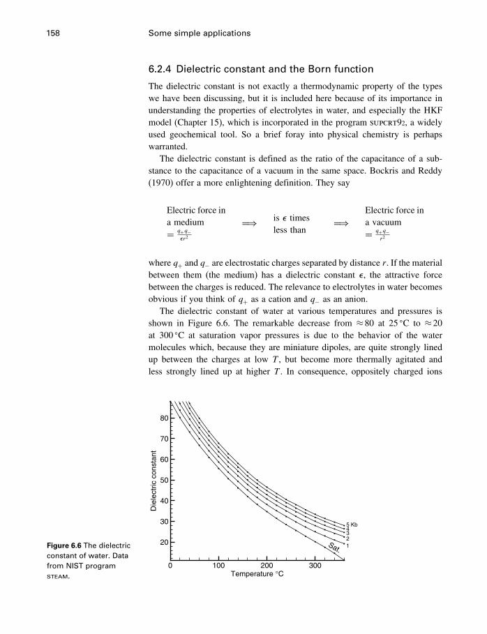
158 Some simple applications
6.2.4 Dielectric constant and the Born function
The dielectric constant is not exactly a thermodynamic property of the typeswe have been discussing, but it is included here because of its importance inunderstanding the properties of electrolytes in water, and especially the HKFmodel (Chapter 15), which is incorporated in the program supcrt92, a widelyused geochemical tool. So a brief foray into physical chemistry is perhapswarranted.
The dielectric constant is defined as the ratio of the capacitance of a sub-stance to the capacitance of a vacuum in the same space. Bockris and Reddy(1970) offer a more enlightening definition. They say
Electric force ina medium= q+q−
�r2
=⇒ is � timesless than
=⇒Electric force ina vacuum= q+q−
r2
where q+ and q− are electrostatic charges separated by distance r. If the materialbetween them (the medium) has a dielectric constant �, the attractive forcebetween the charges is reduced. The relevance to electrolytes in water becomesobvious if you think of q+ as a cation and q− as an anion.
The dielectric constant of water at various temperatures and pressures isshown in Figure 6.6. The remarkable decrease from ≈80 at 25 �C to ≈20at 300 �C at saturation vapor pressures is due to the behavior of the watermolecules which, because they are miniature dipoles, are quite strongly linedup between the charges at low T , but become more thermally agitated andless strongly lined up at higher T . In consequence, oppositely charged ions
Figure 6.6 The dielectricconstant of water. Datafrom NIST programsteam. Temperature °C
Die
lect
ric c
onst
ant
0 100 200 300
20
30
40
50
60
70
80
12345 Kb
Sat.
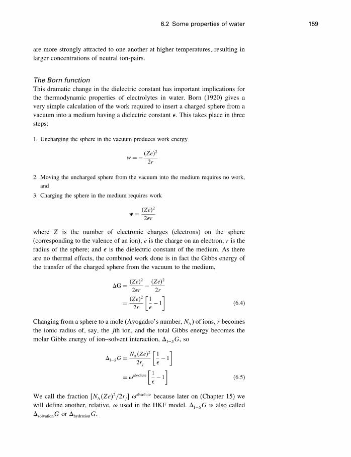
6.2 Some properties of water 159
are more strongly attracted to one another at higher temperatures, resulting inlarger concentrations of neutral ion-pairs.
The Born functionThis dramatic change in the dielectric constant has important implications forthe thermodynamic properties of electrolytes in water. Born (1920) gives avery simple calculation of the work required to insert a charged sphere from avacuum into a medium having a dielectric constant �. This takes place in threesteps:
1. Uncharging the sphere in the vacuum produces work energy
w=− �Ze�2
2r
2. Moving the uncharged sphere from the vacuum into the medium requires no work,
and
3. Charging the sphere in the medium requires work
w= �Ze�2
2�r
where Z is the number of electronic charges (electrons) on the sphere(corresponding to the valence of an ion); e is the charge on an electron; r is theradius of the sphere; and � is the dielectric constant of the medium. As thereare no thermal effects, the combined work done is in fact the Gibbs energy ofthe transfer of the charged sphere from the vacuum to the medium,
�G= �Ze�2
2�r− �Ze�
2
2r
= �Ze�2
2r
[1�−1]
(6.4)
Changing from a sphere to a mole (Avogadro’s number, NA) of ions, r becomesthe ionic radius of, say, the jth ion, and the total Gibbs energy becomes themolar Gibbs energy of ion–solvent interaction, �I−SG, so
�I−SG= NA�Ze�2
2rj
[1�−1]
= �absolute
[1�−1]
(6.5)
We call the fraction [NA�Ze�2/2rj] �
absolute because later on (Chapter 15) wewill define another, relative, � used in the HKF model. �I−SG is also called�solvationG or �hydrationG.
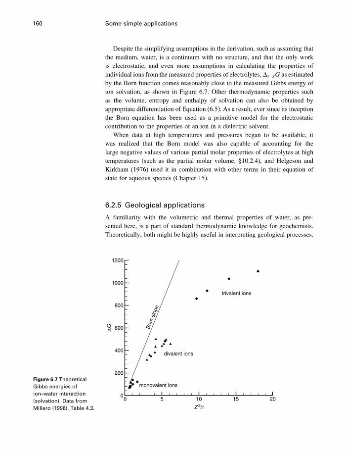
160 Some simple applications
Despite the simplifying assumptions in the derivation, such as assuming thatthe medium, water, is a continuum with no structure, and that the only workis electrostatic, and even more assumptions in calculating the properties ofindividual ions from the measured properties of electrolytes, �I−SG as estimatedby the Born function comes reasonably close to the measured Gibbs energy ofion solvation, as shown in Figure 6.7. Other thermodynamic properties suchas the volume, entropy and enthalpy of solvation can also be obtained byappropriate differentiation of Equation (6.5). As a result, ever since its inceptionthe Born equation has been used as a primitive model for the electrostaticcontribution to the properties of an ion in a dielectric solvent.
When data at high temperatures and pressures began to be available, itwas realized that the Born model was also capable of accounting for thelarge negative values of various partial molar properties of electrolytes at hightemperatures (such as the partial molar volume, §10.2.4), and Helgeson andKirkham (1976) used it in combination with other terms in their equation ofstate for aqueous species (Chapter 15).
6.2.5 Geological applications
A familiarity with the volumetric and thermal properties of water, as pre-sented here, is a part of standard thermodynamic knowledge for geochemists.Theoretically, both might be highly useful in interpreting geological processes.
Figure 6.7 TheoreticalGibbs energies ofion–water interaction(solvation). Data fromMillero (1996), Table 4.3. Z 2/r
∆G
0 5 10 15 200
200
400
600
800
1000
1200
Bor
n sl
ope
monovalent ions
divalent ions
trivalent ions
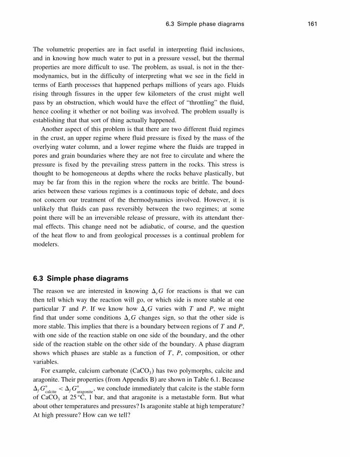
6.3 Simple phase diagrams 161
The volumetric properties are in fact useful in interpreting fluid inclusions,and in knowing how much water to put in a pressure vessel, but the thermalproperties are more difficult to use. The problem, as usual, is not in the ther-modynamics, but in the difficulty of interpreting what we see in the field interms of Earth processes that happened perhaps millions of years ago. Fluidsrising through fissures in the upper few kilometers of the crust might wellpass by an obstruction, which would have the effect of “throttling” the fluid,hence cooling it whether or not boiling was involved. The problem usually isestablishing that that sort of thing actually happened.
Another aspect of this problem is that there are two different fluid regimesin the crust, an upper regime where fluid pressure is fixed by the mass of theoverlying water column, and a lower regime where the fluids are trapped inpores and grain boundaries where they are not free to circulate and where thepressure is fixed by the prevailing stress pattern in the rocks. This stress isthought to be homogeneous at depths where the rocks behave plastically, butmay be far from this in the region where the rocks are brittle. The bound-aries between these various regimes is a continuous topic of debate, and doesnot concern our treatment of the thermodynamics involved. However, it isunlikely that fluids can pass reversibly between the two regimes; at somepoint there will be an irreversible release of pressure, with its attendant ther-mal effects. This change need not be adiabatic, of course, and the questionof the heat flow to and from geological processes is a continual problem formodelers.
6.3 Simple phase diagrams
The reason we are interested in knowing �rG for reactions is that we canthen tell which way the reaction will go, or which side is more stable at oneparticular T and P. If we know how �rG varies with T and P, we mightfind that under some conditions �rG changes sign, so that the other side ismore stable. This implies that there is a boundary between regions of T and P,with one side of the reaction stable on one side of the boundary, and the otherside of the reaction stable on the other side of the boundary. A phase diagramshows which phases are stable as a function of T , P, composition, or othervariables.
For example, calcium carbonate (CaCO3) has two polymorphs, calcite andaragonite. Their properties (from Appendix B) are shown in Table 6.1. Because�fG
�calcite
<�fG�aragonite
, we conclude immediately that calcite is the stable formof CaCO3 at 25 �C, 1 bar, and that aragonite is a metastable form. But whatabout other temperatures and pressures? Is aragonite stable at high temperature?At high pressure? How can we tell?
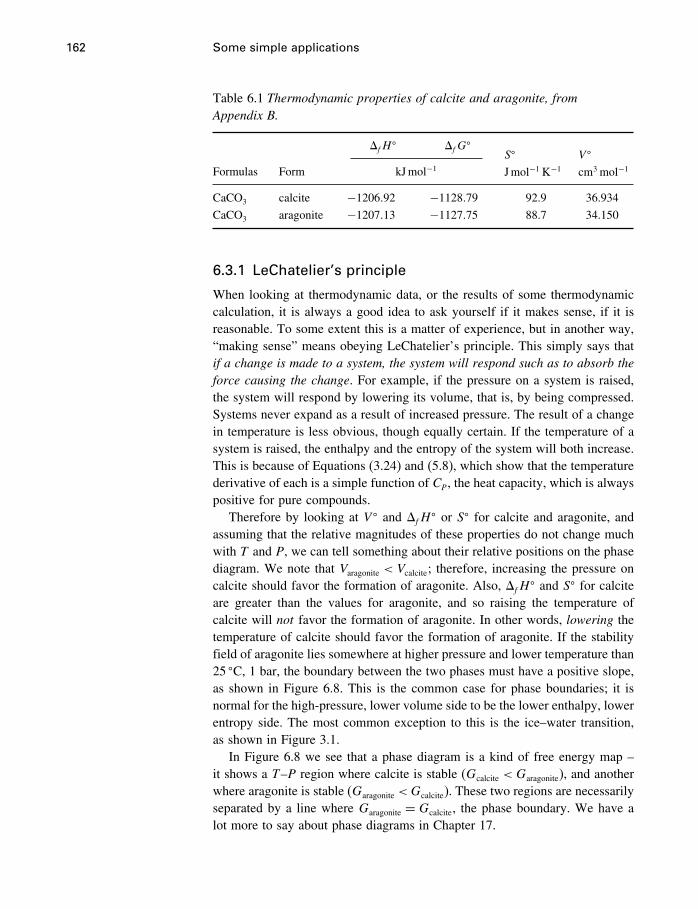
162 Some simple applications
Table 6.1 Thermodynamic properties of calcite and aragonite, fromAppendix B.
�fH� �fG
�S�
Jmol−1 K−1
V �
cm3 mol−1Formulas Form kJmol−1
CaCO3 calcite −1206�92 −1128�79 92.9 36.934
CaCO3 aragonite −1207�13 −1127�75 88.7 34.150
6.3.1 LeChatelier’s principle
When looking at thermodynamic data, or the results of some thermodynamiccalculation, it is always a good idea to ask yourself if it makes sense, if it isreasonable. To some extent this is a matter of experience, but in another way,“making sense” means obeying LeChatelier’s principle. This simply says thatif a change is made to a system, the system will respond such as to absorb theforce causing the change. For example, if the pressure on a system is raised,the system will respond by lowering its volume, that is, by being compressed.Systems never expand as a result of increased pressure. The result of a changein temperature is less obvious, though equally certain. If the temperature of asystem is raised, the enthalpy and the entropy of the system will both increase.This is because of Equations (3.24) and (5.8), which show that the temperaturederivative of each is a simple function of CP, the heat capacity, which is alwayspositive for pure compounds.
Therefore by looking at V � and �fH� or S� for calcite and aragonite, and
assuming that the relative magnitudes of these properties do not change muchwith T and P, we can tell something about their relative positions on the phasediagram. We note that Varagonite < Vcalcite; therefore, increasing the pressure oncalcite should favor the formation of aragonite. Also, �fH
� and S� for calciteare greater than the values for aragonite, and so raising the temperature ofcalcite will not favor the formation of aragonite. In other words, lowering thetemperature of calcite should favor the formation of aragonite. If the stabilityfield of aragonite lies somewhere at higher pressure and lower temperature than25 �C, 1 bar, the boundary between the two phases must have a positive slope,as shown in Figure 6.8. This is the common case for phase boundaries; it isnormal for the high-pressure, lower volume side to be the lower enthalpy, lowerentropy side. The most common exception to this is the ice–water transition,as shown in Figure 3.1.
In Figure 6.8 we see that a phase diagram is a kind of free energy map –it shows a T–P region where calcite is stable (Gcalcite <Garagonite), and anotherwhere aragonite is stable (Garagonite <Gcalcite). These two regions are necessarilyseparated by a line where Garagonite = Gcalcite, the phase boundary. We have alot more to say about phase diagrams in Chapter 17.
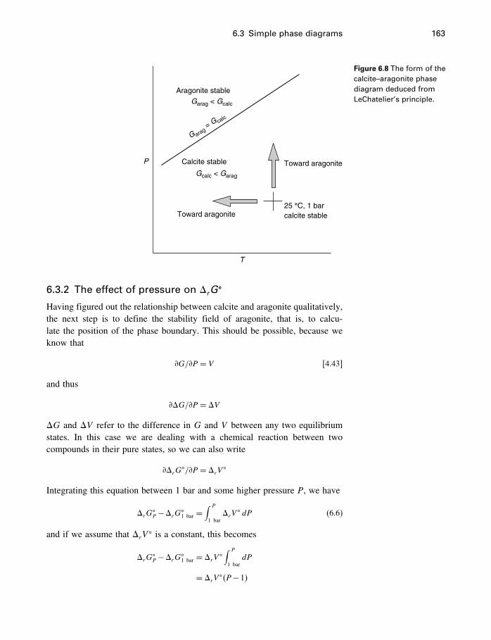
6.3 Simple phase diagrams 163
T
P
Toward aragonite
Toward aragonite
Aragonite stable
Calcite stable
calcite stable
Garag < Gcalc
G arag = G calc
Gcalc < Garag
25 °C, 1 bar
Figure 6.8 The form of thecalcite–aragonite phasediagram deduced fromLeChatelier’s principle.
6.3.2 The effect of pressure on �rG�
Having figured out the relationship between calcite and aragonite qualitatively,the next step is to define the stability field of aragonite, that is, to calcu-late the position of the phase boundary. This should be possible, because weknow that
�G/�P = V [4.43]
and thus
��G/�P = �V
�G and �V refer to the difference in G and V between any two equilibriumstates. In this case we are dealing with a chemical reaction between twocompounds in their pure states, so we can also write
��rG�/�P = �rV �
Integrating this equation between 1 bar and some higher pressure P, we have
�rG�P−�rG�
1 bar =∫ P
1 bar�rV
� dP (6.6)
and if we assume that �rV� is a constant, this becomes
�rG�P−�rG�
1 bar = �rV �∫ P
1 bardP
= �rV ��P−1�
164 Some simple applications
We could use this to evaluate �rG�P at any chosen value of P. However, we
are particularly interested in a value of �rG�P = �rG�
Peqbm= 0, that is, on the
phase boundary. We know the values of
�rG�1 bar = �fG
�aragonite
−�fG�calcite
=−1127�75− �−1128�79�
= 1�04 kJmol−1
= 1040 Jmol−1
and
�rV� = V �
aragonite−V �calcite
= 34�150−36�934
=−2�784 cm3 mol−1
So we can solve the equation for Peqbm, the pressure of the calcite–aragoniteequilibrium at 25 �C.
However, there is one little problem.
The units of volumeVolumes are generally measured in cubic centimeters, milliliters, liters, and soon. But if you look at an equation such as
w =−P �V
you see that we have a problem with our units. Work (w) and P�V are obviouslyenergy terms (Jmol−1), but the product of P in bars and �V in cm3 mol−1 isnot joules. We must always convert our volumes to joules bar−1, so that theproduct of P and V or �V is Jmol−1. The conversion factor (Appendix A) is
1cm3 = 0�10 J bar−1
so now our �rV� is −2�784×0�1=−0�2784 J bar−1.
Now we can solve for pressure Peqbm:
�rG�Peqbm
−�rG�1bar = �rV ��Peqbm −1�
0−1040=−0�2784�Peqbm −1�
Peqbm = 3737 bar
The relationship between G and P in this calculation is shown in Figure 6.9.This gives us one point on the calcite–aragonite phase boundary. We also knowthat the boundary has a positive slope, and so we could sketch a diagramthat would be approximately right, but we really need one more piece ofinformation – either another point on the boundary or its slope.
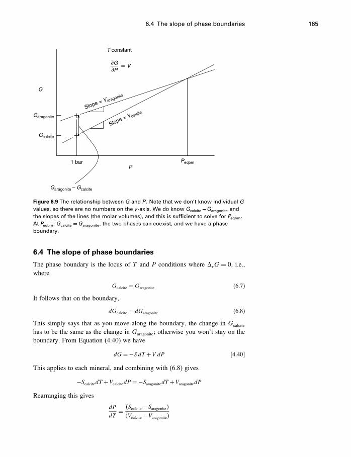
6.4 The slope of phase boundaries 165
G
V∂G∂P
Garagonite – Gcalcite
Garagonite
Gcalcite
1 barP
Peqbm
T constant
Slope = Varagonite
Slope = Vcalcite
Figure 6.9 The relationship between G and P . Note that we don’t know individual Gvalues, so there are no numbers on the y -axis. We do know Gcalcite −Garagonite andthe slopes of the lines (the molar volumes), and this is sufficient to solve for Peqbm.At Peqbm, Gcalcite =Garagonite, the two phases can coexist, and we have a phaseboundary.
6.4 The slope of phase boundaries
The phase boundary is the locus of T and P conditions where �rG = 0, i.e.,where
Gcalcite =Garagonite (6.7)
It follows that on the boundary,
dGcalcite = dGaragonite (6.8)
This simply says that as you move along the boundary, the change in Gcalcite
has to be the same as the change in Garagonite; otherwise you won’t stay on theboundary. From Equation (4.40) we have
dG=−S dT +V dP [4.40]
This applies to each mineral, and combining with (6.8) gives
−ScalcitedT +VcalcitedP =−SaragonitedT +VaragonitedPRearranging this gives
dP
dT= �Scalcite−Saragonite��Vcalcite−Varagonite�
166 Some simple applications
or, for any reaction
dP
dT= �rS
�rV(6.9)
which gives the slope of an equilibrium phase boundary in terms of the entropyand volume changes between the phases involved in the reaction. This is calledthe Clapeyron equation.
Equation (5.1) says
�GT�P = �H−T �S [5.1]
This applies to any change between two equilibrium states at the same T andP. If those two equilibrium states have the same value of G, such as calciteand aragonite do on their phase boundary (6.7), then �GT�P = 0, and
�H = T �S (6.10)
or�H
T= �S (6.11)
This is a useful relationship for any phase boundary,2 which is the usual placeto find �GT�P = 0. This gives an alternative form of the Clapeyron equation,
dP
dT= �H
T �V(6.12)
6.4.1 The slope of the calcite–aragonite boundary
We have one point on the calcite–aragonite boundary at 3737 bar, 25 �C. If weassume that the �rS and the �rV at this P and T are the same as those at 1bar, 25 �C, we can calculate the slope from the data in our tables. Thus
�rS = Saragonite−Scalcite= 88�7−92�9
=−4�2 Jmol−1 K−1 (6.13)
and
�rV = Varagonite−Vcalcite= 34�150−36�934
=−2�784cm3 mol−1
=−0�2784 J bar−1
2 That is, any phase boundary in a one-component system. With two or more components, therelationship is in principle the same but becomes more complicated, and less useful.
6.4 The slope of phase boundaries 167
Therefore
dP
dT= �rS
�rV
= −4�2−0�2784
= 15�09 bar/ �C
Therefore, to get another point on the calcite–aragonite phase boundary,we simply choose an arbitrary temperature increment, say 100 �C, calculatethe corresponding pressure increment, 100×15�09= 1509 bar, and add theseincrements to our first point. We now have a second point at 125 �C, 3737+1509= 5246 bar, and we can plot the boundary as in Figure 6.10.
Keep in mind that we have assumed that the �rS and �rV from the tablesare unchanged at all temperatures and pressures, that is, that they are constants.This is quite a good approximation for a reaction involving only solid phasessuch as this one, but you would not use it for reactions involving liquids,gases, or solutes. In general, all thermodynamic parameters do vary with Tand P, so phase boundaries are in principle curved and not straight as we haveassumed. However, the amount of curvature is quite small in some cases, suchas this one.
6.4.2 Comparison with experimental results
Table 6.2 shows the results of some experiments on the stability of CaCO3 atelevated temperatures and pressures. A mixture of calcite and aragonite was
25 125
5246
3737
1
3737
bar
100 °C 1509
bar
CalciteAragonite
P b
ar
T °C
Figure 6.10 Calculation ofthe calcite–aragonitephase diagram.
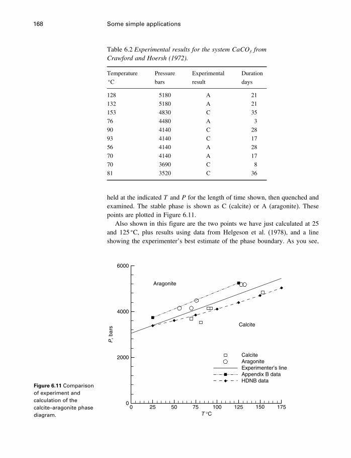
168 Some simple applications
Table 6.2 Experimental results for the system CaCO3 fromCrawford and Hoersh (1972).
Temperature Pressure Experimental Duration�C bars result days
128 5180 A 21
132 5180 A 21
153 4830 C 35
76 4480 A 3
90 4140 C 28
93 4140 C 17
56 4140 A 28
70 4140 A 17
70 3690 C 8
81 3520 C 36
held at the indicated T and P for the length of time shown, then quenched andexamined. The stable phase is shown as C (calcite) or A (aragonite). Thesepoints are plotted in Figure 6.11.
Also shown in this figure are the two points we have just calculated at 25and 125 �C, plus results using data from Helgeson et al. (1978), and a lineshowing the experimenter’s best estimate of the phase boundary. As you see,
Figure 6.11 Comparisonof experiment andcalculation of thecalcite–aragonite phasediagram. T °C
P, b
ars
0 25 50 75 100 125 150 1750
2000
4000
6000
CalciteAragoniteExperimenter’s lineAppendix B dataHDNB data
Aragonite
Calcite
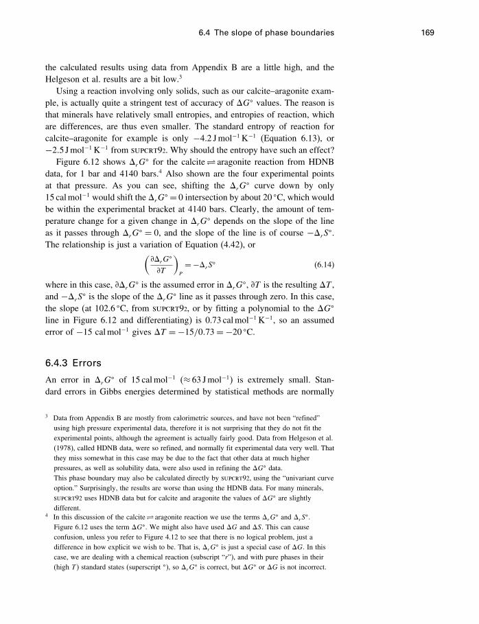
6.4 The slope of phase boundaries 169
the calculated results using data from Appendix B are a little high, and theHelgeson et al. results are a bit low.3
Using a reaction involving only solids, such as our calcite–aragonite exam-ple, is actually quite a stringent test of accuracy of �G� values. The reason isthat minerals have relatively small entropies, and entropies of reaction, whichare differences, are thus even smaller. The standard entropy of reaction forcalcite–aragonite for example is only −4.2 Jmol−1 K−1 (Equation 6.13), or−2�5 Jmol−1 K−1 from supcrt92. Why should the entropy have such an effect?
Figure 6.12 shows �rG� for the calcite� aragonite reaction from HDNB
data, for 1 bar and 4140 bars.4 Also shown are the four experimental pointsat that pressure. As you can see, shifting the �rG
� curve down by only15 calmol−1 would shift the �rG
� = 0 intersection by about 20 �C, which wouldbe within the experimental bracket at 4140 bars. Clearly, the amount of tem-perature change for a given change in �rG
� depends on the slope of the lineas it passes through �rG
� = 0, and the slope of the line is of course −�rS�.The relationship is just a variation of Equation (4.42), or(
��rG�
�T
)P
=−�rS� (6.14)
where in this case, ��rG� is the assumed error in �rG
�, �T is the resulting �T ,and −�rS� is the slope of the �rG
� line as it passes through zero. In this case,the slope (at 102.6 �C, from supcrt92, or by fitting a polynomial to the �G�
line in Figure 6.12 and differentiating) is 0.73 calmol−1 K−1, so an assumederror of −15 calmol−1 gives �T =−15/0�73=−20 �C.
6.4.3 Errors
An error in �rG� of 15 calmol−1 (≈ 63 Jmol−1) is extremely small. Stan-
dard errors in Gibbs energies determined by statistical methods are normally
3 Data from Appendix B are mostly from calorimetric sources, and have not been “refined”using high pressure experimental data, therefore it is not surprising that they do not fit theexperimental points, although the agreement is actually fairly good. Data from Helgeson et al.(1978), called HDNB data, were so refined, and normally fit experimental data very well. Thatthey miss somewhat in this case may be due to the fact that other data at much higherpressures, as well as solubility data, were also used in refining the �G� data.This phase boundary may also be calculated directly by supcrt92, using the “univariant curveoption.” Surprisingly, the results are worse than using the HDNB data. For many minerals,supcrt92 uses HDNB data but for calcite and aragonite the values of �G� are slightlydifferent.
4 In this discussion of the calcite� aragonite reaction we use the terms �rG� and �rS
�.Figure 6.12 uses the term �G�. We might also have used �G and �S. This can causeconfusion, unless you refer to Figure 4.12 to see that there is no logical problem, just adifference in how explicit we wish to be. That is, �rG
� is just a special case of �G. In thiscase, we are dealing with a chemical reaction (subscript “r”), and with pure phases in their(high T ) standard states (superscript �), so �rG
� is correct, but �G� or �G is not incorrect.
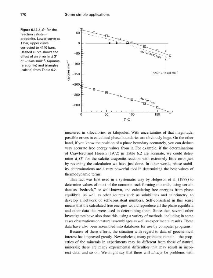
170 Some simple applications
Figure 6.12 �rG� for the
reaction calcite�
aragonite. Lower curve at1 bar, upper curvecorrected to 4140 bars.Dashed curve shows theeffect of an error in �G�
of −15 calmol−1. Squares(aragonite) and triangles(calcite) from Table 6.2.
T °C
calo
ries
mol
–1
0 50 100 150
–300
–250
–200
–150
–100
–50
0
50
∆G ° at 4140 bars
∆G ° at 1 bar
σ∆G ° = 15 cal mol–1
measured in kilocalories, or kilojoules. With uncertainties of that magnitude,possible errors in calculated phase boundaries are obviously huge. On the otherhand, if you know the position of a phase boundary accurately, you can deducevery accurate free energy values from it. For example, if the determinationsof Crawford and Hoersh (1972) in Table 6.2 are accurate, we could deter-mine �rG
� for the calcite–aragonite reaction with extremely little error justby reversing the calculation we have just done. In other words, phase stabil-ity determinations are a very powerful tool in determining the best values ofthermodynamic terms.
This fact was first used in a systematic way by Helgeson et al. (1978) todetermine values of most of the common rock-forming minerals, using certaindata as “bedrock,” or well-known, and calculating free energies from phaseequilibria, as well as other sources such as solubilities and calorimetry, todevelop a network of self-consistent numbers. Self-consistent in this sensemeans that the calculated free energies would reproduce all the phase equilibriaand other data that were used in determining them. Since then several otherinvestigators have also done this, using a variety of methods, including in somecases observations on natural assemblages as well as experimental results. Thesedata have also been assembled into databases for use by computer programs.
Because of these efforts, the situation with regard to data of geochemicalinterest has improved greatly. Nevertheless, many problems remain – the prop-erties of the minerals in experiments may be different from those of naturalminerals; there are many experimental difficulties that may result in incor-rect data, and so on. We might say that there will always be problems with
6.5 Another example 171
data – there will never be complete agreement as to the “best” numbers to use,and there will always be new data to consider.
Accuracy and precisionThe problem will generally be one of accuracy, and not precision. Accuracyrefers to how close to “the truth” your determination is, and precision refersto the dispersion of your determinations – i.e., the reproducibility. Statisticalmethods resulting in “standard errors” refer to precision, but this is no longer aproblem in this field. To illustrate this, consider the case where ten laboratoriescooperate in determining the composition of a sample they wish to establish asa standard. When the results are in, it is found that nine laboratories agree veryclosely, but the tenth gives a very different result. Using standard statisticalmethods, the tenth result can be eliminated as an “outlier,” and the nine resultscombined to give a very impressive “standard error.” However, it may be thatthe tenth result is actually more accurate; that the nine laboratories used somemethod or technique that introduced a systematic error.
The problem of systematic error in analytical and experimental work willalways be with us, which is why there are always arguments about the validity ofvarious methods, and which results are “the best.” Reproducibility is generallyvery good, but who cares, until confidence is established that the accuracyis good. Of course once there is confidence in the methods, measurementsof precision become important in assembling data from various sources, forexample in developing equations of state. Estimates of precision are commonlyused to assign weighting factors to data from different sources.
Thus having self-consistent data is no guarantee, because they may be self-consistent with flawed experiments or analyses. This subject is now a largeand very important part of geochemical research, but it is not particularly athermodynamic subject, so we will not pursue it further here.
6.5 Another example
6.5.1 The effect of temperature on �rG�
To illustrate the effect of temperature on �rG�, we could continue with the
calcite–aragonite case and try to calculate the temperature where the phaseboundary crosses the 1 bar pressure line (Figure 6.10). Unfortunately, thisturns out to be close to absolute zero, so it is not a very useful example.As another case let’s consider the polymorphs of Al2SiO5. There are threeof these, kyanite, andalusite, and sillimanite. Therefore there are three two-phase boundaries, and these three boundaries meet at a single point, whereGkyanite =Gandalusite =Gsillimanite as shown in Figure 6.13. These minerals, whichform quite commonly in rocks subjected to high temperatures and pressuresin the Earth’s crust, are of special interest to geologists who study these rocksbecause the “triple point,” the point where the three phase boundaries meet, is
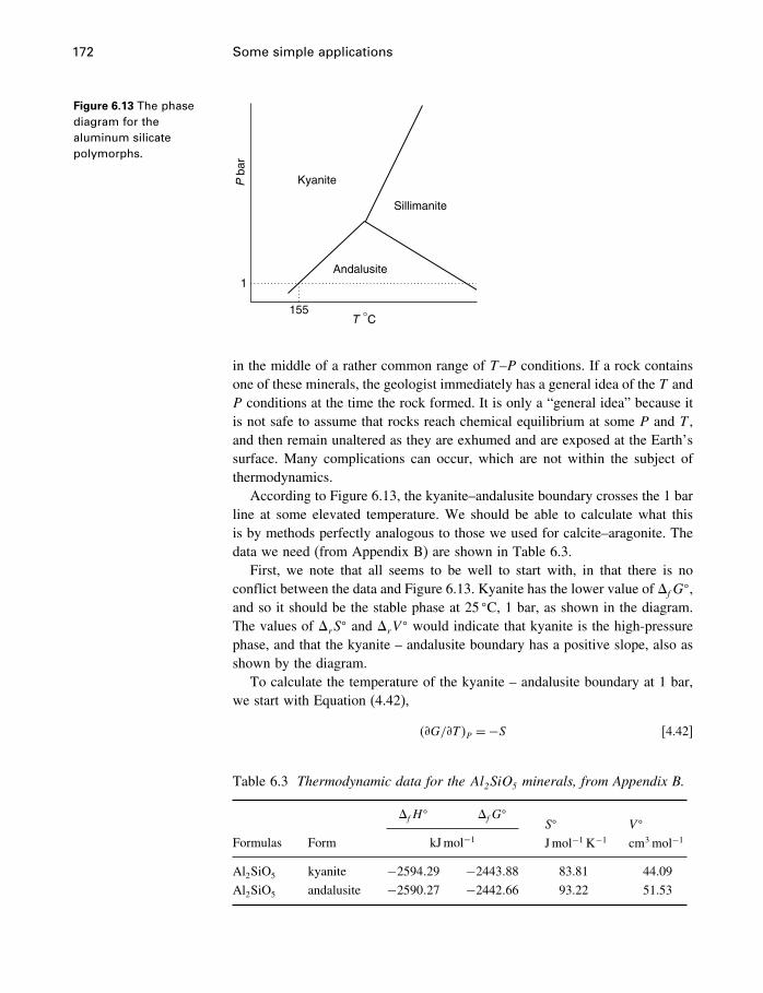
172 Some simple applications
Figure 6.13 The phasediagram for thealuminum silicatepolymorphs.
Kyanite
Sillimanite
Andalusite
P b
ar
1
155T °C
in the middle of a rather common range of T–P conditions. If a rock containsone of these minerals, the geologist immediately has a general idea of the T andP conditions at the time the rock formed. It is only a “general idea” because itis not safe to assume that rocks reach chemical equilibrium at some P and T ,and then remain unaltered as they are exhumed and are exposed at the Earth’ssurface. Many complications can occur, which are not within the subject ofthermodynamics.
According to Figure 6.13, the kyanite–andalusite boundary crosses the 1 barline at some elevated temperature. We should be able to calculate what thisis by methods perfectly analogous to those we used for calcite–aragonite. Thedata we need (from Appendix B) are shown in Table 6.3.
First, we note that all seems to be well to start with, in that there is noconflict between the data and Figure 6.13. Kyanite has the lower value of �fG
�,and so it should be the stable phase at 25 �C, 1 bar, as shown in the diagram.The values of �rS
� and �rV � would indicate that kyanite is the high-pressurephase, and that the kyanite – andalusite boundary has a positive slope, also asshown by the diagram.
To calculate the temperature of the kyanite – andalusite boundary at 1 bar,we start with Equation (4.42),
��G/�T�P =−S [4.42]
Table 6.3 Thermodynamic data for the Al2SiO5 minerals, from Appendix B.
�fH� �fG
�S�
Jmol−1 K−1
V �
cm3 mol−1Formulas Form kJmol−1
Al2SiO5 kyanite −2594�29 −2443�88 83.81 44.09
Al2SiO5 andalusite −2590�27 −2442�66 93.22 51.53
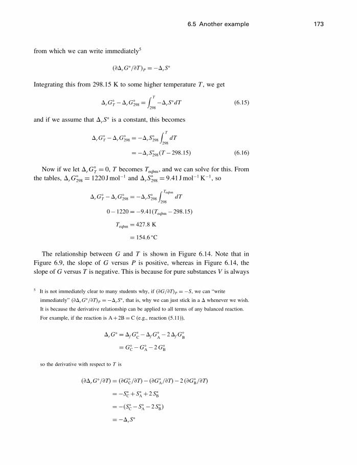
6.5 Another example 173
from which we can write immediately5
���rG�/�T�P =−�rS�
Integrating this from 298.15 K to some higher temperature T , we get
�rG�T −�rG
�298 =
∫ T
298−�rS�dT (6.15)
and if we assume that �rS� is a constant, this becomes
�rG�T −�rG
�298 =−�rS�298
∫ T
298dT
=−�rS�298�T −298�15� (6.16)
Now if we let �rG�T = 0, T becomes Teqbm, and we can solve for this. From
the tables, �rG�298 = 1220 Jmol−1 and �rS
�298 = 9�41 Jmol−1 K−1, so
�rG�T −�rG
�298 =−�rS�298
∫ Teqbm
298dT
0−1220=−9�41�Teqbm −298�15�
Teqbm = 427�8 K
= 154�6 �C
The relationship between G and T is shown in Figure 6.14. Note that inFigure 6.9, the slope of G versus P is positive, whereas in Figure 6.14, theslope ofG versus T is negative. This is because for pure substances V is always
5 It is not immediately clear to many students why, if ��G/�T�P =−S, we can “write
immediately” ���rG�/�T�P =−�rS�, that is, why we can just stick in a � whenever we wish.
It is because the derivative relationship can be applied to all terms of any balanced reaction.
For example, if the reaction is A+2B= C (e.g., reaction (5.11)),
�rG� = �fG
�C−�fG
�A−2�fG
�B
=G�C−G�
A−2G�B
so the derivative with respect to T is
���rG�/�T�= ��G�
C/�T�− ��G�A/�T�−2 ��G�
B/�T�
=−S�C+S�A+2S�B
=−�S�C−S�A−2S�B�
=−�rS�
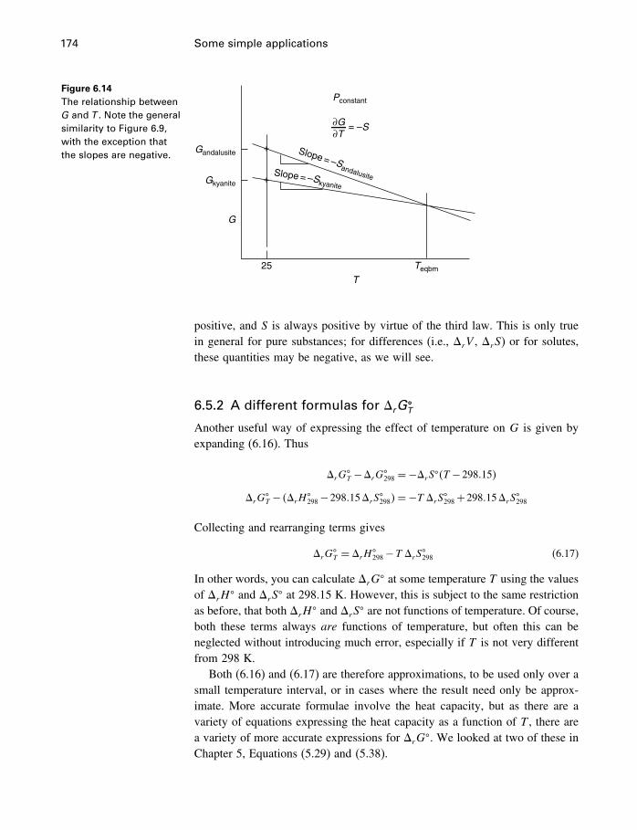
174 Some simple applications
Figure 6.14The relationship betweenG and T . Note the generalsimilarity to Figure 6.9,with the exception thatthe slopes are negative.
25 Teqbm
T
G
Gkyanite
Gandalusite
Pconstant
∂G∂T
= –S
Slope = –SandalusiteSlope = –Skyanite
+
+
positive, and S is always positive by virtue of the third law. This is only truein general for pure substances; for differences (i.e., �rV , �rS) or for solutes,these quantities may be negative, as we will see.
6.5.2 A different formulas for �rG�T
Another useful way of expressing the effect of temperature on G is given byexpanding (6.16). Thus
�rG�T −�rG
�298 =−�rS��T −298�15�
�rG�T − ��rH
�298−298�15�rS
�298�=−T �rS�298+298�15�rS
�298
Collecting and rearranging terms gives
�rG�T = �rH
�298−T �rS�298 (6.17)
In other words, you can calculate �rG� at some temperature T using the values
of �rH� and �rS� at 298.15 K. However, this is subject to the same restriction
as before, that both �rH� and �rS� are not functions of temperature. Of course,
both these terms always are functions of temperature, but often this can beneglected without introducing much error, especially if T is not very differentfrom 298 K.
Both (6.16) and (6.17) are therefore approximations, to be used only over asmall temperature interval, or in cases where the result need only be approx-imate. More accurate formulae involve the heat capacity, but as there are avariety of equations expressing the heat capacity as a function of T , there area variety of more accurate expressions for �rG
�. We looked at two of these inChapter 5, Equations (5.29) and (5.38).
6.6 Summary 175
6.6 Summary
The main idea in this chapter is to illustrate the uses of our thermodynamicvariables, using only pure phases. We did this by considering some propertiesof water at elevated T and P, and by calculating simple phase diagrams. Inphase diagrams, the condition �rG = 0 becomes a central concern, and forpure phases, this is the same as �rG
� = 0.Many reactions involving only pure phases also involve water, but calcu-
lating the Gibbs energy of water at high T and P is more difficult than forminerals, because we cannot assume that it is incompressible. How to han-dle this, as well as how to deal with solutions, is an important topic in laterchapters.
7Ideal solutions
7.1 Introduction
If the world were made of pure substances, our development of the ther-modynamic model would now be complete. We have developed a method,based on measurements of heat flow, that enables predictions to be madeabout which way reactions will go in given circumstances. But one of thereasons that the world is so complex is that pure substances are relativelyrare, and strictly speaking they are nonexistent (even “pure” substances con-tain impurities in trace quantities). Most natural substances are composed ofseveral components, and the result is called a solution. Therefore, we needto develop a way to deal with components in solution in the same way thatwe can now deal with pure substances – we have to be able to get numericalvalues for the Gibbs energies, enthalpies, and entropies of components in solu-tions. We will then be able to predict the outcome of reactions that take placeentirely in solution, such as the ionization of acids and bases, and reactionsthat involve solids and gases as well as dissolved components, such as whetherminerals will dissolve or precipitate. Our thermodynamic model will then becomplete.
In this chapter we have a look at how to deal with dissolved substances –solutes. When we mix two substances together, sometimes they dissolve intoone another, like sugar into coffee or alcohol into water, and sometimes theydo not, like oil and water. In the former case, if we thought about it at all, wewould probably expect that the properties of the mixture or solution would besome kind of average of the properties of the two separate substances. Thisis more or less true for some properties, but decidedly not true for the mostimportant one, Gibbs energy.
After making sure we understand how to express the composition of solu-tions, we begin by considering properties of ideal solutions, which are, asyou might expect, the simplest possible properties that solutions might have.As you might also expect, no real solutions are in fact ideal, although somecome fairly close. But the properties of ideal solutions are of interest not onlybecause some solutions are almost ideal, but because what we often do formore complex solutions is to subtract the properties of the ideal solution from
176
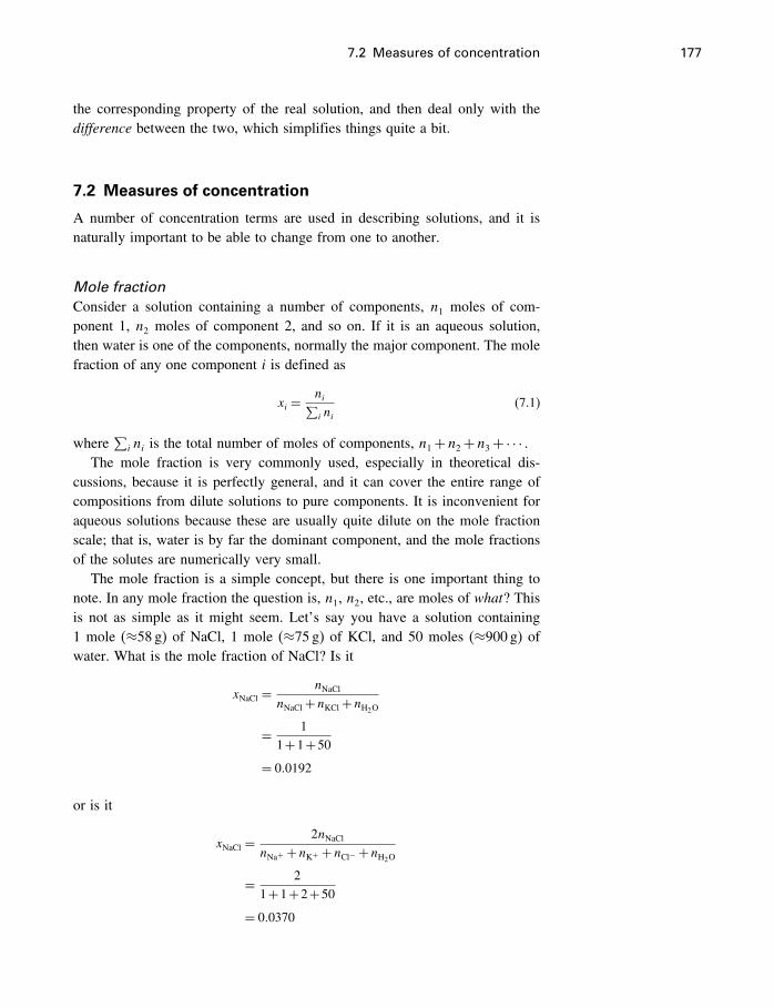
7.2 Measures of concentration 177
the corresponding property of the real solution, and then deal only with thedifference between the two, which simplifies things quite a bit.
7.2 Measures of concentration
A number of concentration terms are used in describing solutions, and it isnaturally important to be able to change from one to another.
Mole fractionConsider a solution containing a number of components, n1 moles of com-ponent 1, n2 moles of component 2, and so on. If it is an aqueous solution,then water is one of the components, normally the major component. The molefraction of any one component i is defined as
xi =ni∑i ni
(7.1)
where∑i ni is the total number of moles of components, n1+n2+n3+· · · .
The mole fraction is very commonly used, especially in theoretical dis-cussions, because it is perfectly general, and it can cover the entire range ofcompositions from dilute solutions to pure components. It is inconvenient foraqueous solutions because these are usually quite dilute on the mole fractionscale; that is, water is by far the dominant component, and the mole fractionsof the solutes are numerically very small.
The mole fraction is a simple concept, but there is one important thing tonote. In any mole fraction the question is, n1, n2, etc., are moles of what? Thisis not as simple as it might seem. Let’s say you have a solution containing1 mole (≈58 g) of NaCl, 1 mole (≈75 g) of KCl, and 50 moles (≈900 g) ofwater. What is the mole fraction of NaCl? Is it
xNaCl =nNaCl
nNaCl+nKCl+nH2O
= 11+1+50
= 0�0192
or is it
xNaCl =2nNaCl
nNa+ +nK+ +nCl− +nH2O
= 21+1+2+50
= 0�0370
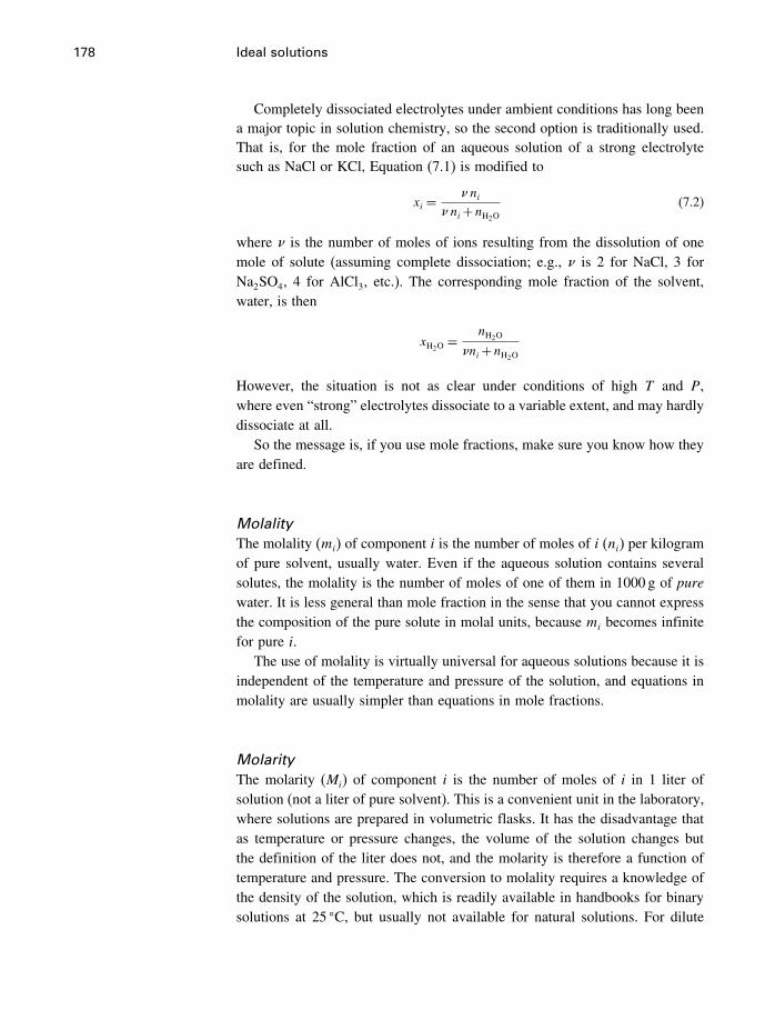
178 Ideal solutions
Completely dissociated electrolytes under ambient conditions has long beena major topic in solution chemistry, so the second option is traditionally used.That is, for the mole fraction of an aqueous solution of a strong electrolytesuch as NaCl or KCl, Equation (7.1) is modified to
xi =� ni
� ni+nH2O(7.2)
where � is the number of moles of ions resulting from the dissolution of onemole of solute (assuming complete dissociation; e.g., � is 2 for NaCl, 3 forNa2SO4, 4 for AlCl3, etc.). The corresponding mole fraction of the solvent,water, is then
xH2O= nH2O
�ni+nH2O
However, the situation is not as clear under conditions of high T and P,where even “strong” electrolytes dissociate to a variable extent, and may hardlydissociate at all.
So the message is, if you use mole fractions, make sure you know how theyare defined.
MolalityThe molality (mi) of component i is the number of moles of i (ni) per kilogramof pure solvent, usually water. Even if the aqueous solution contains severalsolutes, the molality is the number of moles of one of them in 1000 g of purewater. It is less general than mole fraction in the sense that you cannot expressthe composition of the pure solute in molal units, because mi becomes infinitefor pure i.
The use of molality is virtually universal for aqueous solutions because it isindependent of the temperature and pressure of the solution, and equations inmolality are usually simpler than equations in mole fractions.
MolarityThe molarity (Mi) of component i is the number of moles of i in 1 liter ofsolution (not a liter of pure solvent). This is a convenient unit in the laboratory,where solutions are prepared in volumetric flasks. It has the disadvantage thatas temperature or pressure changes, the volume of the solution changes butthe definition of the liter does not, and the molarity is therefore a function oftemperature and pressure. The conversion to molality requires a knowledge ofthe density of the solution, which is readily available in handbooks for binarysolutions at 25 �C, but usually not available for natural solutions. For dilute
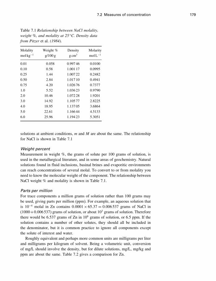
7.2 Measures of concentration 179
Table 7.1 Relationship between NaCl molality,weight %, and molality at 25 �C. Density datafrom Pitzer et al. (1984).
Molality Weight % Density Molarity
mol kg−1 g/100 g g cm3 molL−1
0.01 0�058 0.997 46 0.0100
0.10 0�58 1.001 17 0.0995
0.25 1�44 1.007 22 0.2482
0.50 2�84 1.017 10 0.4941
0.75 4�20 1.026 76 0.7377
1.0 5�52 1.036 23 0.9790
2.0 10�46 1.072 28 1.9201
3.0 14�92 1.105 77 2.8225
4.0 18�95 1.137 05 3.6864
5.0 22�61 1.166 44 4.5133
6.0 25�96 1.194 23 5.3051
solutions at ambient conditions, m and M are about the same. The relationshipfor NaCl is shown in Table 7.1
Weight percentMeasurement in weight %, the grams of solute per 100 grams of solution, isused in the metallurgical literature, and in some areas of geochemistry. Naturalsolutions found in fluid inclusions, basinal brines and evaporitic environmentscan reach concentrations of several molal. To convert to or from molality youneed to know the molecular weight of the component. The relationship betweenNaCl weight % and molality is shown in Table 7.1.
Parts per millionFor trace components a million grams of solution rather than 100 grams maybe used, giving parts per million (ppm). For example, an aqueous solution thatis 10−4 molal in Zn contains 0�0001× 65�37 = 0�006537 grams of NaCl in(1000+0�006537) grams of solution, or about 103 grams of solution. Thereforethere would be 6.537 grams of Zn in 106 grams of solution, or 6.5 ppm. If thesolution contains a number of other solutes, they should all be included inthe denominator, but it is common practice to ignore all components exceptthe solute of interest and water.
Roughly equivalent and perhaps more common units are milligrams per literand milligrams per kilogram of solvent. Being a volumetric unit, conversionof mg/L should involve the density, but for dilute solutions, mg/L, mg/kg andppm are about the same. Table 7.2 gives a comparison for Zn.
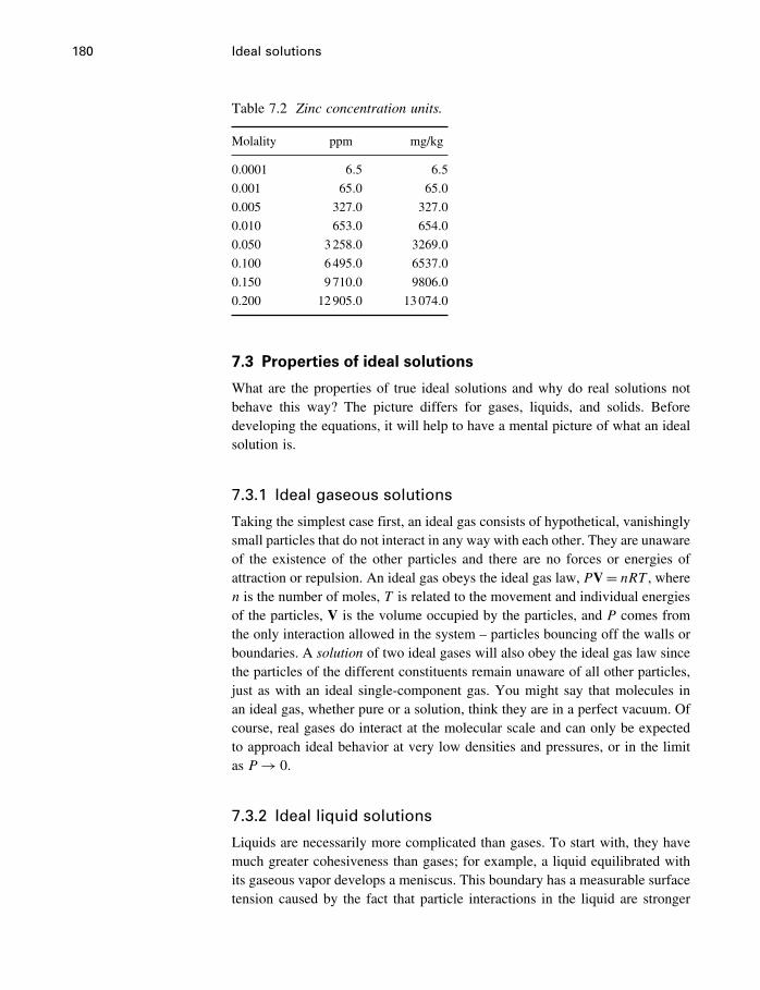
180 Ideal solutions
Table 7.2 Zinc concentration units.
Molality ppm mg/kg
0.0001 6�5 6�5
0.001 65�0 65�0
0.005 327�0 327�0
0.010 653�0 654�0
0.050 3258�0 3269�0
0.100 6495�0 6537�0
0.150 9710�0 9806�0
0.200 12905�0 13074�0
7.3 Properties of ideal solutions
What are the properties of true ideal solutions and why do real solutions notbehave this way? The picture differs for gases, liquids, and solids. Beforedeveloping the equations, it will help to have a mental picture of what an idealsolution is.
7.3.1 Ideal gaseous solutions
Taking the simplest case first, an ideal gas consists of hypothetical, vanishinglysmall particles that do not interact in any way with each other. They are unawareof the existence of the other particles and there are no forces or energies ofattraction or repulsion. An ideal gas obeys the ideal gas law, PV= nRT , wheren is the number of moles, T is related to the movement and individual energiesof the particles, V is the volume occupied by the particles, and P comes fromthe only interaction allowed in the system – particles bouncing off the walls orboundaries. A solution of two ideal gases will also obey the ideal gas law sincethe particles of the different constituents remain unaware of all other particles,just as with an ideal single-component gas. You might say that molecules inan ideal gas, whether pure or a solution, think they are in a perfect vacuum. Ofcourse, real gases do interact at the molecular scale and can only be expectedto approach ideal behavior at very low densities and pressures, or in the limitas P→ 0.
7.3.2 Ideal liquid solutions
Liquids are necessarily more complicated than gases. To start with, they havemuch greater cohesiveness than gases; for example, a liquid equilibrated withits gaseous vapor develops a meniscus. This boundary has a measurable surfacetension caused by the fact that particle interactions in the liquid are stronger
7.3 Properties of ideal solutions 181
than those in the vapor. A liquid must have significant interaction among itsparticles – if it did not, it would disperse and become a gas.
In an ideal liquid solution, the forces of interaction between all molecules,whether of one type or another, are exactly the same. For example in a liquidsolution of constituents A and B, interactions A–A, A–B, and B–B must beidentical. This means that all constituents A,B,…, must have the same molecularproperties (size, charge, polarity, bonding characteristics). This is never thecase, of course, but mixtures of some organic compounds come fairly close.
Given this uniformity of intermolecular forces in the ideal liquid solution(as opposed to the absence of such forces in the ideal gas), it follows that manyproperties of the solution are very simply related to the properties of the purecompounds. Thus the volume of the solution is the sum of the volumes of thepure components before mixing, and no heat is absorbed or given off when thesolution is prepared (because such effects are caused by changes in the particleinteractions, which we have just ruled out).
7.3.3 Ideal solid solutions
A solid has a rigid structure, and its component molecules, ions, or atomsare confined to specific structural sites. The regularity of the structure varies,of course, from glassy to fully crystalline materials, but whatever the degreeof ordering, the positions of the particles are fixed. Whereas ideal gases andgaseous solutions have a complete absence of interparticle forces and idealliquid solutions have a complete uniformity, solids must have highly specificinteractions between different constituents. We speak of specific sites in crys-tals, such as tetrahedral silicon–oxygen bonds and octahedral aluminum sites,and the same is true (although to a lesser extent) of glassy solids. The inter-actions between Si–Si, Si–O, Si–Al, O–O, and Al–O in an aluminosilicate areall quite different. However, within the framework of a perfectly crystallinecompound it is frequently possible to substitute one element for another. Thissubstitution and the corresponding solid solution would be ideal if the twosubstituting elements or species were completely indistinguishable. The clos-est approximation to an ideal solid solution would be the substitution of twoisotopes of the same element on the same crystal site. Like ideal gaseousand liquid solutions, there would be no heat evolved on mixing the compo-nents and the total volume of the solution must simply be the sum of thevolumes of the pure constituents before mixing. We go into more detail inChapter 14.
7.3.4 Two kinds of ideal solution
There is only one kind of ideal gas solution, as discussed above, but there aretwo kinds of ideal liquid and solid solutions.
182 Ideal solutions
Our discussion of liquid and solid solution ideality above makes no provisionfor the possibility that there might be more than one definition of ideality; thata solution might act ideally in one way but not in another. If in a liquid solutionof A and B there are A–A and A–B interactions but no B–B interactions wehave another kind of ideal solution, in which changing the concentration of Bresults in a perfectly linear change in the properties of B, and has no effect onthe properties of A. In order for there to be no B–B interaction, particles ofB must be quite widely separated – the concentration of B in A must be verysmall. This leads to the concept of the “infinitely dilute solution,” in whichthere is only one particle of B in a sea of A, and therefore there is interactionbetween the particle of B and the surrounding A, and of course A–A interaction,but here being no other B particles, there is no B–B interaction. We can’t dealwith a single molecule of B, so we need to think of a mole of B particles andhave so much A that no B particle is influenced by another B particle – perhapsa roomful of A, as in the room analogy on page 278.
These two kinds of ideality permeate discussions of liquid and solid solutionproperties, and are formalized by two ideal solution laws – Raoult’s law andHenry’s law.
7.4 Ideal solution laws
These relationships or laws were discovered in the nineteenth century byinvestigations of gas or vapor pressures associated with solutions of knowncomposition. Because the gas or vapor was at a fairly low pressure, it acted asan ideal gas, and because it was in equilibrium with the solution, it providedinformation on the nature of the liquid solution. Today, the original connectionwith an associated vapor or gas phase is a secondary concern. The relationshipbetween the ideal solution components themselves proves to be more useful,a subject to be discussed in terms of activities, an important topic introducedhere and treated more fully in Chapter 8. Before discussing these relationships,we look first at solutions of ideal gases.
7.4.1 Dalton’s law
The simplest imaginable system other than a vacuum is undoubtedly an idealgas. One mole of ideal gas occupies 22.41 liters at 0 �C, 1 atm, so that (fromthe ideal gas law) one mole of ideal gas occupying one liter at 0 �C would havea pressure of 22.41 bars.
It was an early discovery (Dalton, 1811) that mixtures of gases would exerta pressure equal to the sum of the pressures that each of the species gaseswould have if each alone occupied the same volume. This was establishedusing gases at relatively low pressures where they behave close to ideally, and
7.4 Ideal solution laws 183
in fact it is only strictly true for mixtures of ideal gases, which are also thenideal gases. Thus for each species gas 1, 2, 3, etc.
P1V= n1RTP2V= n2RTetc…
and for the gas mixture
PtotalV=∑i
niRT
Thus
P1
Ptotal= n1∑
i ni= x1
P2
Ptotal= n2∑
i ni= x2
etc…
or,
P1 = x1 ·Ptotal
P2 = x2 ·Ptotal
������
etc…
⎫⎪⎪⎪⎪⎪⎪⎪⎪⎬⎪⎪⎪⎪⎪⎪⎪⎪⎭(7.3)
P1, P2, etc., are called the partial pressures of the solution gases andequations (7.3) are now normally used as the definition of partial pressure eventhough in real, nonideal solutions they give a quantity that is not equivalent tothe original meaning, i.e., the pressure a gas would exert if it alone occupiedthe total volume.1
7.4.2 Henry’s law
Henry’s law in its original form stated that the solubility of a gas in a liquidis proportional to the pressure on the gas. In Figure 7.1 is shown an apparatusfor controlling the pressure on a gas i in contact with a liquid. As the pressureon the gas Pi increases, more of it dissolves in the liquid, and so xi increases.When xi is sufficiently small, it is directly proportional to Pi, and the constant
1 There are several definitions of partial pressure. deHeer (1986, §23.4) says there are five, andexplains the three most common. In my experience, only the definition in Equations (7.3) isever used in geochemistry.
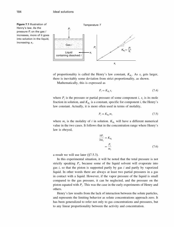
184 Ideal solutions
Figure 7.1 Illustration ofHenry’s law. As thepressure Pi on the gas i
increases, more of it goesinto solution in the liquid,increasing xi .
Gas i
Liquidcontaining dissolved i
xi
xixi
Pi
Pi
Temperature T
KHi=
Pi
of proportionality is called the Henry’s law constant, KHi. As xi gets larger,
there is inevitably some deviation from strict proportionality, as shown.Mathematically, this is expressed as
Pi = KHixi (7.4)
where Pi is the pressure or partial pressure of some component i, xi is its molefraction in solution, and KHi
is a constant, specific for component i, the Henry’slaw constant. Actually, it is more often used in terms of molality,
Pi = KHimi (7.5)
where mi is the molality of i in solution. KHiwill have a different numerical
value in the two cases. It follows that in the concentration range where Henry’slaw is obeyed,
�Pi�mi
= KHi
= Pimi
(7.6)
a result we will use later (§7.5.3).In this experimental situation, it will be noted that the total pressure is not
strictly speaking Pi, because some of the liquid solvent will evaporate intogas i, so that the piston is supported partly by gas i and partly by vaporizedliquid. In other words there are always at least two partial pressures in a gasin contact with a liquid. However, if the vapor pressure of the liquid is smallcompared to the gas pressure, it can be neglected, and the pressure on thepiston equated with Pi. This was the case in the early experiments of Henry andothers.
Henry’s law results from the lack of interaction between the solute particles,and represents the limiting behavior as solute concentrations approach zero. Ithas been generalized to refer not only to gas concentrations and pressures, butto any linear proportionality between the activity and concentration.
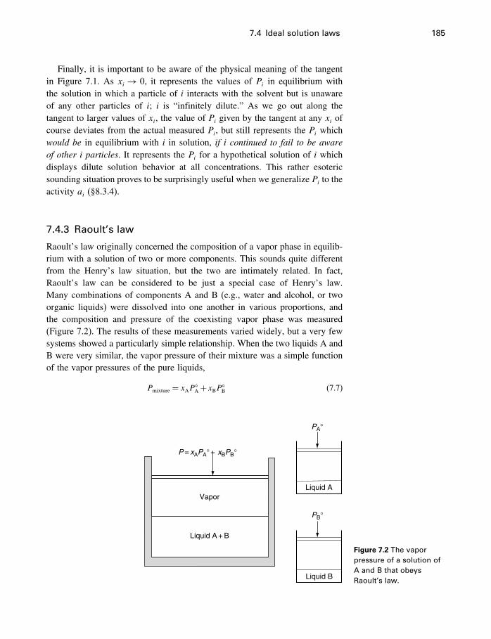
7.4 Ideal solution laws 185
Finally, it is important to be aware of the physical meaning of the tangentin Figure 7.1. As xi → 0, it represents the values of Pi in equilibrium withthe solution in which a particle of i interacts with the solvent but is unawareof any other particles of i; i is “infinitely dilute.” As we go out along thetangent to larger values of xi, the value of Pi given by the tangent at any xi ofcourse deviates from the actual measured Pi, but still represents the Pi whichwould be in equilibrium with i in solution, if i continued to fail to be awareof other i particles. It represents the Pi for a hypothetical solution of i whichdisplays dilute solution behavior at all concentrations. This rather esotericsounding situation proves to be surprisingly useful when we generalize Pi to theactivity ai (§8.3.4).
7.4.3 Raoult’s law
Raoult’s law originally concerned the composition of a vapor phase in equilib-rium with a solution of two or more components. This sounds quite differentfrom the Henry’s law situation, but the two are intimately related. In fact,Raoult’s law can be considered to be just a special case of Henry’s law.Many combinations of components A and B (e.g., water and alcohol, or twoorganic liquids) were dissolved into one another in various proportions, andthe composition and pressure of the coexisting vapor phase was measured(Figure 7.2). The results of these measurements varied widely, but a very fewsystems showed a particularly simple relationship. When the two liquids A andB were very similar, the vapor pressure of their mixture was a simple functionof the vapor pressures of the pure liquids,
Pmixture = xAP�A+xBP�
B (7.7)
Liquid A + B
Vapor
P = xAPA° xBPB°+
PA°
PB°
Liquid A
Liquid B
Figure 7.2 The vaporpressure of a solution ofA and B that obeysRaoult’s law.
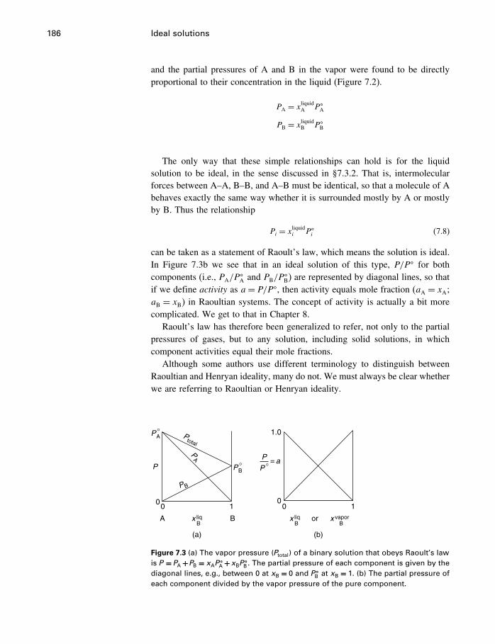
186 Ideal solutions
and the partial pressures of A and B in the vapor were found to be directlyproportional to their concentration in the liquid (Figure 7.2).
PA = xliquidA P�A
PB = xliquidB P�B
The only way that these simple relationships can hold is for the liquidsolution to be ideal, in the sense discussed in §7.3.2. That is, intermolecularforces between A–A, B–B, and A–B must be identical, so that a molecule of Abehaves exactly the same way whether it is surrounded mostly by A or mostlyby B. Thus the relationship
Pi = xliquidi P�i (7.8)
can be taken as a statement of Raoult’s law, which means the solution is ideal.In Figure 7.3b we see that in an ideal solution of this type, P/P� for bothcomponents (i.e., PA/P
�A and PB/P
�B) are represented by diagonal lines, so that
if we define activity as a= P/P�, then activity equals mole fraction (aA = xA;aB = xB) in Raoultian systems. The concept of activity is actually a bit morecomplicated. We get to that in Chapter 8.
Raoult’s law has therefore been generalized to refer, not only to the partialpressures of gases, but to any solution, including solid solutions, in whichcomponent activities equal their mole fractions.
Although some authors use different terminology to distinguish betweenRaoultian and Henryan ideality, many do not. We must always be clear whetherwe are referring to Raoultian or Henryan ideality.
A B
(a) (b)
0 1 000
1
1.0
P °B
P °A
x liqB
x liqB
x vaporB
P
or
PB
PA
Ptotal
P
P °= a
Figure 7.3 (a) The vapor pressure (Ptotal) of a binary solution that obeys Raoult’s lawis P = PA +PB = xAP
�A +xBP
�B. The partial pressure of each component is given by the
diagonal lines, e.g., between 0 at xB = 0 and P �B at xB = 1. (b) The partial pressure of
each component divided by the vapor pressure of the pure component.

7.5 Ideal solution equations 187
7.5 Ideal solution equations
7.5.1 Volume, enthalpy, heat capacity
These terms are simply additive in ideal solutions. Volume is the most intuitiveof these terms, and we illustrate the additivity of volumes in ideal solutions in§10.2.1. This leads to Equation (10.4), the generalized form of which is
Videal sol’n =∑i
xiV�i (7.9)
where V is the molar volume of an ideal solution, and V �i is the molar volume
of the pure component i.The form of Equation (7.9) applies also to any thermodynamic parameter
which does not contain entropy in its definition. The important ones are enthalpyand heat capacity, so that
Hideal sol’n =∑i
xiH�i (7.10)
and
CP ideal sol’n =∑i
xiCP�i (7.11)
The difference between the property of a solution and the combined proper-ties of the pure components is called a mixing property. For an ideal solution,from Equations (7.9)–(7.11)
�mixVideal sol’n = Videal sol’n−∑i
xiV�i (7.12)
=(��mixG
�P
)T
= 0
�mixHideal sol’n =Hideal sol’n−∑i
xiH�i (7.13)
=(��mixG/T
��1/T�
)P
= 0
�mixCP ideal sol’n = CP ideal sol’n−∑i
xiCP�i (7.14)
=(��mixH
�T
)P
= 0
7.5.2 Entropy, Gibbs energy
Entropy and other potential quantities which contain entropy (such as G) arespecifically defined so as to change in spontaneous processes, and two or more
188 Ideal solutions
substances dissolving into one another is a perfect example of a spontaneousprocess.
Consider two ideal gases which are allowed to mix at constant P and T . Inthe final mixture, which is also an ideal gas, the partial pressure of gas 1 isP1 = x1P, and of gas 2 is P2 = x2P, where x1 and x2 are the mole fractions. Thechange in entropy on mixing, �mixS, is equal to the �S involved in expandingeach gas from its initial pressure P to its partial pressure in the gas mixture.From Equation (5.41), this process is, for each gas
�S1 = R ln�P/P1�
and
�S2 = R ln�P/P2�
and the total change in entropy is
�mixSideal sol’n = x1R ln�P/P1�+x2R ln�P/P2�
= x1R ln�1/x1�+x2R ln�1/x2�
=−R�x1 ln x1+x2 ln x2� (7.15)
or, in general terms,
�mixSideal sol’n = Sideal sol’n−∑i
xiS�i (7.16)
=−R∑i
xi ln xi (7.17)
=−(��mixG
�T
)P
(7.18)
Because the x terms are fractional, �mixSideal sol’n is inherently positive.Equation (7.17) can also be derived from reasonably simple statistical consid-erations which have nothing to do with the physical state of the particles. Inother words it applies equally to ideal gas, liquid, and solid solutions.
It is important to note the fundamental difference between the ideal mixingof volumes and other terms not containing entropy (Equations 7.9, 7.10, 7.11),which are just linear combinations of the pure end-member terms, and theideal entropy of mixing, Equations (7.16), (7.17), which are nonlinear, andresult in all mixtures having a higher entropy than points on the
∑i xiS
�i line
or plane. It is this property which gives the entropy, Gibbs energy and otherthermodynamic potentials (all of which contain an entropy term, either as partof the definition or as a constraint) their ability to predict energy differences,and hence reaction directions.
7.5 Ideal solution equations 189
The Gibbs paradox
Equation (7.17) has resulted in a quite remarkable literature on what is called “the
Gibbs paradox.” Consider the case of two gases, A and B. The mixing expression
for −�S/R is then �xA ln xA +xB ln xB�. Gibbs pointed out (Gibbs, Dover 1961
edition, p. 166), using slightly different expressions, that this is independent of
the nature of the gases,
…except that the gases which are mixed must be of different kinds. If we
should bring into contact two masses of the same kind of gas, they would
also mix, but there would be no increase in entropy.
This situation, which Gibbs explains on the same page, has been discussed by
innumerable authors, often on a molecular or statistical basis. The best treatment,
I think, is by E.T. Jaynes (1992). He says that
Usually, Gibbs’ prose style conveys his meaning in a sufficiently clear
way, using no more than twice as many words as Poincaré or Einstein
would have used to say the same thing.
but that on this point he is more than usually obscure, although perfectly right.
Jaynes then examines the case where, unknown to us, there are actually two
different kinds of argon, Ar1 and Ar2, identical in all respects, except that Ar2
is soluble in Whifnium, while Ar1 is not. Whifnium is one of the rare superkalic
elements; in fact, it is so rare that it has not yet been discovered. Until the
discovery of Whifnium in the next century, we would not know there were such
things as Ar1 and Ar2, and even if by chance we happened to mix Ar1 and Ar2
we would have no way of knowing that they were two different entities, and we
would correctly describe the mixing process as having zero change in entropy.
After the discovery of Whifnium, we can prepare pure Ar1 and Ar2, and carry out
the same mixing process, and we can even suppose that every molecule follows
exactly the same path that might have happened previously by pure chance (when
we knew nothing about Ar1 and Ar2). But in this case the entropy change is
given by Equation (7.17), and is nonzero, perfectly illustrating why there is a
paradox. Jaynes then goes on to discuss Whafnium, in which Ar1 is soluble but
Ar2 is not.
In his usual elegant style, Jaynes uses this situation to clarify not only the
macroscopic nature of thermodynamics, but the role of information, reversible
and irreversible mixing and the work available. Particularly interesting is his use
of this example to emphasize the importance of defining the constraints (which
he calls macrovariables) defining a system. When we know about Ar1 and Ar2
and are able to separate them by doing work on the system, we have an extra
constraint in the sense of §4.9.2.
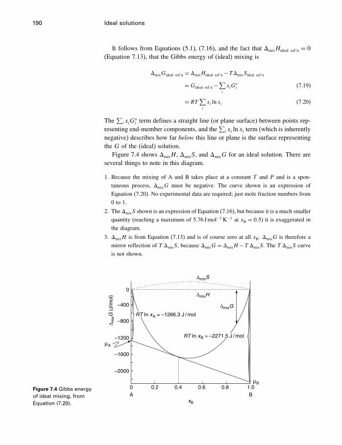
190 Ideal solutions
It follows from Equations (5.1), (7.16), and the fact that �mixHideal sol’n = 0(Equation 7.13), that the Gibbs energy of (ideal) mixing is
�mixGideal sol’n = �mixHideal sol’n−T�mixSideal sol’n
=Gideal sol’n−∑i
xiG�i (7.19)
= RT∑i
xi ln xi (7.20)
The∑i xiG
�i term defines a straight line (or plane surface) between points rep-
resenting end-member components, and the∑i xi ln xi term (which is inherently
negative) describes how far below this line or plane is the surface representingthe G of the (ideal) solution.
Figure 7.4 shows �mixH , �mixS, and �mixG for an ideal solution. There areseveral things to note in this diagram.
1. Because the mixing of A and B takes place at a constant T and P and is a spon-
taneous process, �mixG must be negative. The curve shown is an expression of
Equation (7.20). No experimental data are required; just mole fraction numbers from
0 to 1.
2. The �mixS shown is an expression of Equation (7.16), but because it is a much smaller
quantity (reaching a maximum of 5.76 Jmol−1 K−1 at xB = 0�5) it is exaggerated in
the diagram.
3. �mixH is from Equation (7.13) and is of course zero at all xB. �mixG is therefore a
mirror reflection of T �mixS, because �mixG= �mixH−T �mixS. The T �mixS curve
is not shown.
Figure 7.4 Gibbs energyof ideal mixing, fromEquation (7.20).
0 0.2 0.4 0.6 0.8 1.0A B
xB
–2000
–1600
–1200
–800
–400
0
µB
µA
∆ mixG
(J/
mol
)
RT In xA = –1266.3 J / mol
RT In xB = –2271.5 J / mol
∆mixH
∆mixS
∆mixG
7.5 Ideal solution equations 191
4. We don’t have absolute values for G, so we must always measure the difference in
G from some other state at the same T and P. In Figure 7.4 this other state is pure
A (xA = 1) and pure B (xB = 1).
5. Despite appearances, the molar Gibbs energy curve in Figure 7.4 is actually asymp-
totic to each vertical axis, whereas the volume curve in Figure 10.2 is not. This is
not of great importance by itself, but it is connected to the fact that we cannot use
the infinite dilution standard state for Gibbs energy. We leave this important topic
to Chapter 8.
Chemical potentialsFigure 7.4 also introduces us to a new problem. Because the mixing curve isconcave downward, the Gibbs energies of components A and B in the solutionare necessarily less than the corresponding values of G�
A and G�B, the molar
Gibbs energies of the pure compounds. The fact that this is so provides the(thermodynamic) reason why A and B form a solution. If we mix nA moles ofA and nB moles of B the reaction is
nA A+nB B= �nA A� nB B�solution (7.21)
and the Gibbs energy change for this reaction is �mixG, which is negative.During this reaction, the Gibbs energy of both A and B become lower. If themixing line lies above the straight line joining G�
A and G�B, then �Gmix would
be positive, the dissolution reaction (7.21) would not be spontaneous, and nosolution would form – A and B would be immiscible, like oil and water.
So GsolutionA < G�
A, and GsolutionB < G�
B. But this raises a few questions, likewhat are these quantities Gsolution
A and GsolutionB ? Where are they on the diagram?
How can you separate �Gmix into these two separate quantities? If we knowthat, then perhaps we could evaluate G�
A−GsolutionA and G�
A−GsolutionA .
You can see by simple inspection of Figure 7.4 that at any point on the�mixG curve, the tangent at that point allows calculation of the numerical valueof that point on the curve by combining two points on the tangent in a linearcombination. In Figure 7.4 we show the tangent to the curve at xB = 0�4, andidentify the intersections of the tangent with the two ordinate axes as �A and�B. In Equation (7.19) we see that ifG
�A andG�
B are zero, then �mixG=Gsolution,and in drawing Figure 7.4, this is exactly what we have assumed. We have made�mixG the difference between the G of the solution and zero. Evidently then,
Gsolution = xA�A+xB�B (7.22)
But what is the physical meaning of �? There are two ways of answering this.
Euler’s answerMathematically minded people simply invoke Euler’s theorem for homoge-neous functions (§C.2.3). In plain language, this says that for any extensive
192 Ideal solutions
(total) function such as V or in this case G, having nA moles of component Aand nB moles of component B
G= nA(�G�nA
)nB
+nB(�G�nB
)nA
(7.23)
or, dividing by �nA+nB�,
G= xA(�G�nA
)nB
+xB(�G�nB
)nA
(7.24)
Comparing (7.22) and (7.24), we have
�A =(�G�nA
)T�P�nB
�B =(�G�nB
)T�P�nA
⎫⎪⎪⎪⎬⎪⎪⎪⎭ (7.25)
so the tangent intersections are in fact the partial derivatives of the total Gibbsenergy of the solution G with respect to nA and nB. These are in fact ourfirst examples of partial molar terms, introduced in §2.4.1 and §4.14.1. � isa partial molar Gibbs energy, and it is our answer to the question, what is theGibbs energy per mole of a dissolved substance? It is important to develop anintuitive understanding of partial molar terms, so we devote quite a bit morediscussion to this in Chapter 10.
Our answerBut we don’t have to use Euler’s theorem. We can simply expand our definitionof G, which so far is restricted to closed (constant composition) systems. If weexclude chemical work, which means we deal only with systems at completestable equilibrium, we know from Equation (4.65)
dG=−SdT +VdP+∑i
�idni
At constant T and P [by implication a condition of Equations (7.23) and (7.24)]the first two terms on the right drop out, and integrating the other terms froman increment of solution up to the whole system, we get, for two components1 and 2,
G= n1(�G�n1
)T�P�n1
+n2(�G�n2
)T�P�n2
which is Equation (7.23), and from there we get Equations (7.25) again.So that answers one question–how do we split Gsolution into Gsolution
A andGsolution
B , and where are these things on the diagram? The next question is, howdo we evaluate G�
A−GsolutionA and G�
B−GsolutionB ?
7.5 Ideal solution equations 193
7.5.3 The relation between composition and free energy
Figure 7.4 also shows a very important relationship between Gibbs energy andcomposition, namely, that
�A−G�A = RT ln xA
�B−G�B = RT ln xB
⎫⎬⎭ (7.26)
Equations (7.26) provide a relationship between the concentration of anideal solution component and its Gibbs energy. This is an important milestone.Equations (4.42) and (4.43)
��G/�T�P =−S [4.42]
��G/�P�T = V [4.43]
showed how Gibbs energy varies with T and P, respectively (expanded upon inFigures 6.9, 6.14); now we can see how Gibbs energy varies with concentrationof something in solution. If we can calculate the Gibbs energy of solids, liquids,gases, and solutes over a range of T , P, and composition (x), we have justabout solved all our problems, in principle. Basically, from here on we willbe amplifying and coming to grips with practical matters, such as the fact thatEquation (7.26) only applies to Raoultian solutions.
But where do Equations (7.26) come from?
Gibbs energy and mole fraction IThe most direct way to derive the relationship between Gibbs energy and molefraction is to simply differentiate the total form of Equation (7.20) with respectto ni. For two components, G = G/�n1 + n2�, so multiplying both sides of(7.20) by �n1+n2�, then differentiating, gives
�
�n1�Gsol’n−n1G�
1−n2G�2�=
�
�n1�RT �n1 ln x1+n2 ln x2��
which, with n2, G�1, and G
�2 constant, gives
�1−G�1 = RT
[�
�n1�n1 ln x1�+
�
�n1�n2 ln �1−x1��
]= RT �ln x1+x2−x2�= RT ln x1 (7.27)
which is (7.26) for component 1.Applying the same method to Equation (7.15) we get
Si−S�i =−R ln xi (7.28)
and recall that �mixH = 0, so
Hi−H�i = 0 (7.29)
194 Ideal solutions
as well, for ideal solutions.There is a complication in (7.27) and (7.28) which is actually very general
but will only become important in the study of solid solutions (Chapter 14).We discuss it in more detail in §9.10.2, but briefly, the problem is that inEquation (7.27) the left side is a difference in energy per mole, which obviouslydepends on how the mole is defined, but the right side has a mole fraction,which is independent of the definition of the mole as long as all componentsof the solution are treated in the same way.
For example, normally we define a mole of nitrogen as Avogadro’s numberof N2 in nitrogen gas, and oxygen as O2. But we could define these as thesame number of N and O, or of N4 and O4, without affecting the mole fraction.Whether these forms exist or not is not relevant. The mole fraction of N2 in asolution of nitrogen and oxygen does not depend on which of these ways wedefine the mole, but the value of � does. Avogadro’s number of N4 particleshas twice the mass and twice the energy of the same number of N2 particles,so
�N4−��
N4= 2��N2
−��N2� (7.30)
Therefore, if there is any question as to the size of the mole, which usu-ally only arises in defining components in solid solutions, Equation (7.27) isgeneralized to
�1−G�1 = nRT ln x1
= RT ln xnx1 (7.31)
where n is the factor relating the two definitions of the mole.
Gibbs energy and mole fraction IIIt will also prove useful to derive (7.27) another way, especially when we usemolal units of concentration instead of mole fractions. So first we will re-derive(7.27), and then use the same method for molal units in §8.2.3.
Equation (7.27) expresses the relationship between� and x, or concentration.To derive this, it would seem natural to find an expression for the derivativeof � with a concentration term, and then integrate. In other words, what isthe value of ���i/�ni�ni? How does �i (the G of i in solution) vary with theamount of i in solution in the ideal case? This is a partial derivative, so if niis the number of moles of i, we need to keep the concentrations of all othercomponents constant. We denote all other components by ni.
If we expand ���i/�ni�T�P�ni by introducing Pi, the pressure on gaseous iwhich is, or might be, in equilibrium with solute i (whether or not there is sucha gas phase is irrelevant), we get(
��i�ni
)ni
= ��i�Pi
�Pi�ni
(7.32)
7.5 Ideal solution equations 195
where �i is the same in the solution and in the (perhaps hypothetical) gas phase,where it can be called Gi (the gas being assumed ideal), so that ���i/�Pi� =��Gi/�Pi� = Vi = RT/Pi, and where ��Pi/�ni� = Pi/ni is an expression ofHenry’s law (Equation 7.6).2 Combining all this we get(
��i�ni
)ni
= RT
ni(7.33)
for ideal solutions. Integrating this equation between two values of ni, n′i and
n′′i , we get
�′′i −�′
i = RT lnn′′in′i
= RT lnP ′′i
P ′i
by Henry’s law
�′′i −��
i = RT lnP ′′i
P�i
if state ′ is pure i
and, from Equation (7.8)
�i−��i = RT ln xi (state ′′ no longer needs superscript) (7.34)
which is Equation (7.26) for component i.When xB = 0�4 and xA = 0�6, R= 8�31451 Jmol−1 K−1, and T = 298�15K,
Equation (7.26) gives
�A−G�A =−1266 Jmol−1
and
�B−G�B =−2271 Jmol−1
This says that a mole of A has 1266 Jmol−1 less in the dissolved state than inthe pure state, and this is the “thermodynamic explanation” for why A dissolvesin B.
Constructing the tangentsAlthough not essential to understanding the thermodynamics involved, it is ofsome interest to know how to calculate the position of the tangents and thechemical potential intercepts in Figure 7.4.
2 OK, Equation (7.6) shows the ratio of Pi to mi, not ni. But as mi is just ni per kilogram ofsolvent, the ratio is the same.
196 Ideal solutions
The tangent is the slope of the curve calculated from Equation (7.20).Therefore the equation for the slope of the tangent is (not forgetting thatxA = 1−xB) (
d�mixG
dxB
)= d
dxB�RT�xA ln xA+xB ln xB��
= RT ln(xBxA
)(7.35)
and the equation for the tangent line itself is
�A = �mixG−xB(d�mixG
dxB
)(7.36)
If you substitute (7.35) into (7.36) you get, not surprisingly, �A = RT ln xA,which is Equation (7.26), except that we take �� = 0 in the diagram. This maymake the whole thing look like an exercise in algebra. Well, it is, but it isalgebra that is exceptionally useful as a basis for understanding solutions.
7.6 Next step – the activity
We have now developed the relationship between the Gibbs energy of a com-ponent of a solution and the concentration of that component (Equations 7.26,7.27, 7.34). However, it only applies to ideal solutions, and only for concentra-tions in mole fractions. Obviously we need to expand the range of applicabilityof this relationship.
Doing this gets complicated, because we have gaseous, liquid and solidsolutions, a variety of concentration scales, nonideal solutions, and severaldifferent standard states that �� refers to. That is, the quantity �i−��
i need notalways refer to the difference between i in solution and i in its pure state. Atthe same time, the form of Equation (7.34) is very convenient, and we want toretain it for all these conditions. We do this by defining the activity, alreadymentioned in §7.4.3, as
�i−��i = RT lnai (7.37)
All the complications are accommodated by this parameter, and we try to sortit all out in Chapter 8.
7.7 Summary
In Chapter 4 (§4.12.1) we saw that
��G/�T�P =−S [4.42]
and
��G/�P�T = V [4.43]
7.7 Summary 197
We didn’t bother to write, though it is equally true, that
��G/�T�P =−S (7.38)
and
��G/�P�T = V (7.39)
and, differentiating by ni, that
��S/�ni�T�P = Si (7.40)
and
��V/�ni�T�P = Vi (7.41)
meaning that any solution property, not just Gibbs energy, can be split up intothe contributions of the individual components. Finally, because
�
�T
(�G�ni
)= �
�ni
(�G�T
)and similarly for P, then
��i�T
=−Si
and
��i�P
= Vi
So it turns out that
���i/�T�P�n =−Si���i/�P�T�n = Vi
���/�ni�T�P�ni = RT/ni
⎫⎪⎪⎪⎬⎪⎪⎪⎭ (7.42)
are the relationships we need to be able to evaluate (by integration) to knowthe Gibbs energy of any substance as a function of T , P, and composition.But we’re not finished yet. The first two equations apply to any solution, butthe ���/�ni� equation deals only with ideal solutions. We need to find waysto evaluate the partial molar properties in the first two equations, and how tomodify the third one so that it works for any solution. We do this in Chapter 10.A central concept in all of this is the activity, which we take up in Chapter 8.
8Fugacity and activity
8.1 Fugacity
8.1.1 Introduction
The fugacity was introduced by G.N. Lewis in 1901, and became widely usedafter the appearance of Thermodynamics, a very influential textbook by Lewisand Randall in 1923. Lewis describes the need for such a function in terms of ananalogy with temperature in the attainment of equilibrium between phases. Justas equilibrium requires that heat must flow such that temperature is the samein all parts of the system, so matter must flow such that chemical potentials arealso equalized. He referred to the flow of matter from one phase to another asan “escaping tendency,” such as a liquid escaping to the gas form to achievean equilibrium vapor pressure. He pointed out that in fact vapor pressure isequilibrated between phases under many conditions (and in fact is the basis forthe isopiestic method of activity determinations, §5.8.4), and could serve as agood measure of escaping tendency if it behaved always as an ideal gas.
The chemical potential is of course another measure of “escaping tendency,”but Lewis pointed out that there are “certain respects in which this functionis awkward.” This refers to the fact that �→−� as a→ 0, because activityis defined as �−�� = RT lna. Lewis defined a function which would bemuch like a vapor pressure, which would be equilibrated between phases atequilibrium, even in nonideal cases, and even if no vapor phase actually existed.It is an absolute property, in the sense that it does not depend on a standardstate, and it has units of pressure. Lewis and Randall (1923) called it a kind of“ideal or corrected vapor pressure.”
Fugacity has proved useful in a number of ways. One way is to providea relatively simple way to evaluate the integral
∫VdP. In §5.7.1 we saw one
way to do this. That is, for solids, we often assume that the molar volumeis constant, making the integration very simple. Another way, for gases, is toassume the ideal gas law (see below). This is actually a special case of themost general method, which is to develop an equation of state for the system(Chapter 13), from which you can generate all its thermodynamic properties.
Lacking an equation of state, how do we evaluate the pressure integral fora fluid such as H2O or CO2, either in the pure form, mixed with other fluid
198
8.1 Fugacity 199
components, or reacting with solid phases? A possible way to proceed wouldbe to express V as a function of P in some sort of power series, just as we didfor CP as a function of T (Equation 3.26).
∫V dP could then be integrated, and
we could determine the values of the power series coefficients for each gas orfluid and tabulate them as we do for the Maier–Kelley coefficients.
8.1.2 Definition of fugacity
Fortunately, thanks to the insight of Lewis, we can proceed in a simpler andcompletely different fashion. To see how the inspiration for such a functionmight have arisen, consider the form of the volume integral
∫V dP for an ideal
gas. Starting with (4.43),
dG= V dP
= RT
PdP
= RTd lnP (8.1)∫ P2
P1
dG=∫ P2
P1
RT
PdP
GP2 −GP1 = RT lnP2
P1(8.2)
If P1 is 1 bar and this is designated a standard or reference state denoted bya superscript �, then P2 becomes simply P, and
G−G� = RT lnP
P�
= RT lnP since P� = 1 (8.3)
Thus for ideal gases RT lnP all by itself gives the value of∫ PP=1 dG. Unfortu-
nately, this doesn’t work for real gases although it’s not a bad approximation atlow pressures and high temperatures where real gases approach ideal behavior.However, the form of the relationship
dG= V dP = RT d lnP
(Equation 8.1) is sufficient to suggest that we could define a function such thatthe relationship would hold true for real gases. This function is the fugacity,f , where
dG= V dP = RTd ln f (8.4)
200 Fugacity and activity
and ∫ P2
P1
dG=∫ P2
P1
V dP
GP2 −GP1 =∫ P2
P1
RT d ln f
= RT lnfP2fP1
(8.5)
Because f appears as a ratio in (8.5), this equation cannot serve as a fulldefinition of f . We must specify how to determine the fugacity at some Pand T , then the integral can be used to calculate it at other pressures at thatT . To complete the definition, it would be convenient for f to approximateP for gases that behave more or less ideally, that is, at low values of P. Weaccomplish this by stipulating that
limP→0
(f
P
)= 1 (8.6)
This means that for an ideal gas, f = P, and for gases at low pressures, f ≈ P.Equations (8.6) plus (8.4) or (8.5) make up the definition of fugacity.
Fugacity coefficientThe ratio f/P is called the fugacity coefficient, f . Thus
fi = fiP (8.7)
where P is the pressure of a pure fluid compound, or the partial pressure ofa compound in a solution. The partial pressure is a measure of concentration,so the fugacity coefficient is another kind of activity coefficient, introducedin §10.6.1.
8.1.3 Calculation of fugacity
From the preceding equations we see that to measure fugacity, we need to knowthe molar volume as a function of P. In other words we have to measure gasdensities. Also we should measure these densities down to very low pressures –pressures sufficiently low that we can say f =P to whatever degree of accuracyis required. But at these low pressures, the volume of a given mass of gasbecomes very large and very difficult to measure accurately. Thus, while inprinciple evaluating
∫V dP is straightforward, in practice it is difficult when
the lower limit of integration is a very low pressure. To avoid evaluating thisintegral at very low pressures where V → �, it is convenient to define aresidual function , where
= V real−V ideal gas (8.8)
= V −RT/P
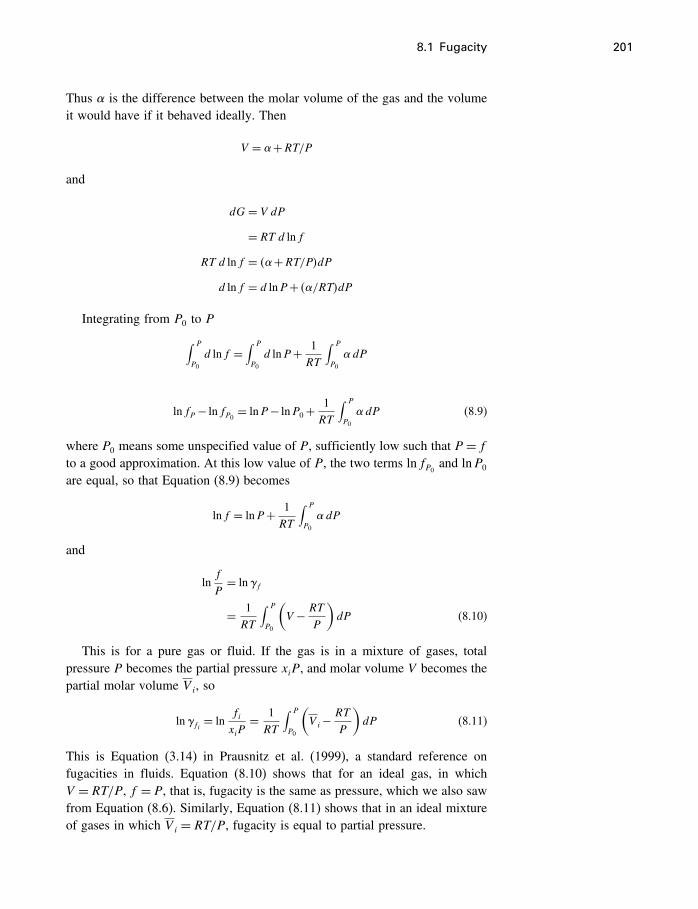
8.1 Fugacity 201
Thus is the difference between the molar volume of the gas and the volumeit would have if it behaved ideally. Then
V = +RT/P
and
dG= V dP= RT d ln f
RT d ln f = �+RT/P�dPd ln f = d lnP+ �/RT�dP
Integrating from P0 to P∫ P
P0
d ln f =∫ P
P0
d lnP+ 1RT
∫ P
P0
dP
ln fP− ln fP0 = lnP− lnP0+1RT
∫ P
P0
dP (8.9)
where P0 means some unspecified value of P, sufficiently low such that P = fto a good approximation. At this low value of P, the two terms ln fP0 and lnP0
are equal, so that Equation (8.9) becomes
ln f = lnP+ 1RT
∫ P
P0
dP
and
lnf
P= lnf
= 1RT
∫ P
P0
(V − RT
P
)dP (8.10)
This is for a pure gas or fluid. If the gas is in a mixture of gases, totalpressure P becomes the partial pressure xiP, and molar volume V becomes thepartial molar volume V i, so
lnfi = lnfixiP
= 1RT
∫ P
P0
(V i−
RT
P
)dP (8.11)
This is Equation (3.14) in Prausnitz et al. (1999), a standard reference onfugacities in fluids. Equation (8.10) shows that for an ideal gas, in whichV = RT/P, f = P, that is, fugacity is the same as pressure, which we also sawfrom Equation (8.6). Similarly, Equation (8.11) shows that in an ideal mixtureof gases in which V i = RT/P, fugacity is equal to partial pressure.
202 Fugacity and activity
Equation (8.11) has P and T as independent variables. More commonly,however, P is known as some function of V and T . In this case Equation (8.11)becomes
lnfi = lnfixiP
= 1RT
∫ �
V
[(�P
�ni
)− RTP
]dV −RT lnZ (8.12)
where Z is the compressibility factor (§13.2.4). This is Equation (3.53) inPrausnitz et al. (1999).
BecauseZ−1P
= V −RT/PRT
we can rewrite Equation (8.10) as
lnf =∫ P
P0
�Z−1�d lnP (8.13)
so the fugacity coefficient can be calculated as a function of Z, the compress-ibility factor, and since Z is known and is the same for most gases in termsof their Pr and Tr , then f/P can be calculated for any gas given its Pc and Tc.Several authors have prepared charts showing f/P as a function of Pr at variousTr . This is a useful device for obtaining fugacities of gases in the lower rangeof geologically interesting P–T conditions. The charts do not extend far intothe metamorphic range of P–T conditions, but nevertheless the compressibilityfactor has found very wide use in equations of state and other treatments offugacity.
The Lewis fugacity ruleIn Chapter 7 we saw that if substances mix ideally (�mV = 0),
V = xA V �A+xB V �
B �10�4�
This volumetric ideal mixing is known as Amagat’s law. If substances mixnonideally (�mV �= 0),
V = xA VA+xB VB �10�7�
It follows, because (10.7) is perfectly general, that for ideal solutions, the partialmolar volume is the same as the molar volume, Vi = V i. Therefore, comparing(8.10) and (8.11), we see that
f pure
P= fmix
xiP
or
fmixi = xi ·f pure (8.14)
This is the Lewis fugacity rule, and is seen to be true if Amagat’s law is true.So fluids can mix ideally volumetrically, but might still be nonideal mixtures.Note that it assumes the additivity of the molar volumes of all components of
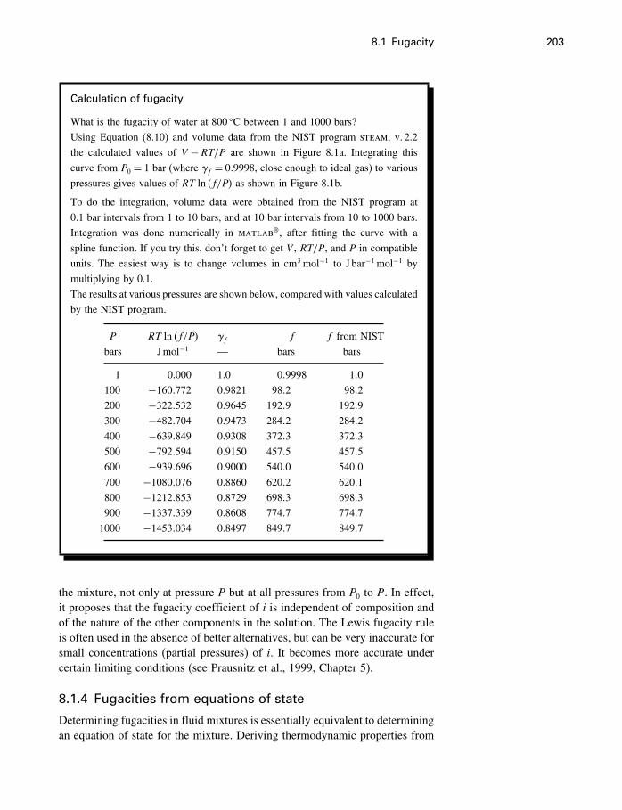
8.1 Fugacity 203
Calculation of fugacity
What is the fugacity of water at 800 �C between 1 and 1000 bars?
Using Equation (8.10) and volume data from the NIST program steam, v. 2.2
the calculated values of V −RT/P are shown in Figure 8.1a. Integrating this
curve from P0 = 1 bar (where f = 0�9998, close enough to ideal gas) to various
pressures gives values of RT ln �f/P� as shown in Figure 8.1b.
To do the integration, volume data were obtained from the NIST program at
0.1 bar intervals from 1 to 10 bars, and at 10 bar intervals from 10 to 1000 bars.
Integration was done numerically in matlab®, after fitting the curve with a
spline function. If you try this, don’t forget to get V , RT/P, and P in compatible
units. The easiest way is to change volumes in cm3 mol−1 to J bar−1 mol−1 by
multiplying by 0.1.
The results at various pressures are shown below, compared with values calculated
by the NIST program.
P RT ln �f/P� f f f from NIST
bars Jmol−1 — bars bars
1 0.000 1.0 0�9998 1�0
100 −160�772 0.9821 98�2 98�2
200 −322�532 0.9645 192�9 192�9
300 −482�704 0.9473 284�2 284�2
400 −639�849 0.9308 372�3 372�3
500 −792�594 0.9150 457�5 457�5
600 −939�696 0.9000 540�0 540�0
700 −1080�076 0.8860 620�2 620�1
800 −1212�853 0.8729 698�3 698�3
900 −1337�339 0.8608 774�7 774�7
1000 −1453�034 0.8497 849�7 849�7
the mixture, not only at pressure P but at all pressures from P0 to P. In effect,it proposes that the fugacity coefficient of i is independent of composition andof the nature of the other components in the solution. The Lewis fugacity ruleis often used in the absence of better alternatives, but can be very inaccurate forsmall concentrations (partial pressures) of i. It becomes more accurate undercertain limiting conditions (see Prausnitz et al., 1999, Chapter 5).
8.1.4 Fugacities from equations of state
Determining fugacities in fluid mixtures is essentially equivalent to determiningan equation of state for the mixture. Deriving thermodynamic properties from
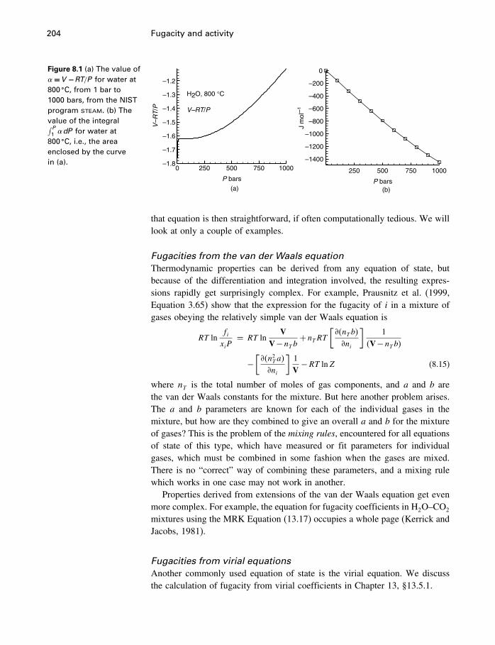
204 Fugacity and activity
Figure 8.1 (a) The value of�= V −RT/P for water at800 �C, from 1 bar to1000 bars, from the NISTprogram steam. (b) Thevalue of the integral∫ P
1 �dP for water at800 �C, i.e., the areaenclosed by the curvein (a).
V–R
T/P
P bars
–1.8
–1.7
–1.6
–1.5
–1.4
–1.3
–1.2
0 250 500 750 1000
H2O, 800 °C
V–RT/P
(a)
J m
ol–1
P bars
250 500 750 1000
–1400
–1200
–1000
–800
–600
–400
–200
0
(b)
that equation is then straightforward, if often computationally tedious. We willlook at only a couple of examples.
Fugacities from the van der Waals equationThermodynamic properties can be derived from any equation of state, butbecause of the differentiation and integration involved, the resulting expres-sions rapidly get surprisingly complex. For example, Prausnitz et al. (1999,Equation 3.65) show that the expression for the fugacity of i in a mixture ofgases obeying the relatively simple van der Waals equation is
RT lnfixiP
= RT lnV
V−nTb+nTRT
[��nTb�
�ni
]1
�V−nTb�
−[��n2Ta�
�ni
]1V−RT lnZ (8.15)
where nT is the total number of moles of gas components, and a and b arethe van der Waals constants for the mixture. But here another problem arises.The a and b parameters are known for each of the individual gases in themixture, but how are they combined to give an overall a and b for the mixtureof gases? This is the problem of the mixing rules, encountered for all equationsof state of this type, which have measured or fit parameters for individualgases, which must be combined in some fashion when the gases are mixed.There is no “correct” way of combining these parameters, and a mixing rulewhich works in one case may not work in another.
Properties derived from extensions of the van der Waals equation get evenmore complex. For example, the equation for fugacity coefficients in H2O–CO2
mixtures using the MRK Equation (13.17) occupies a whole page (Kerrick andJacobs, 1981).
Fugacities from virial equationsAnother commonly used equation of state is the virial equation. We discussthe calculation of fugacity from virial coefficients in Chapter 13, §13.5.1.
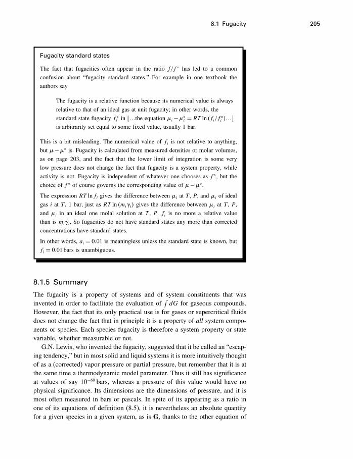
8.1 Fugacity 205
Fugacity standard states
The fact that fugacities often appear in the ratio f/f � has led to a common
confusion about “fugacity standard states.” For example in one textbook the
authors say
The fugacity is a relative function because its numerical value is always
relative to that of an ideal gas at unit fugacity; in other words, the
standard state fugacity f �i in […the equation �i−��i = RT ln �fi/f
�i �…]
is arbitrarily set equal to some fixed value, usually 1 bar.
This is a bit misleading. The numerical value of fi is not relative to anything,
but �−�� is. Fugacity is calculated from measured densities or molar volumes,
as on page 203, and the fact that the lower limit of integration is some very
low pressure does not change the fact that fugacity is a system property, while
activity is not. Fugacity is independent of whatever one chooses as f �, but thechoice of f � of course governs the corresponding value of �−��.
The expression RT ln fi gives the difference between �i at T , P, and �i of ideal
gas i at T , 1 bar, just as RT ln �mii� gives the difference between �i at T , P,
and �i in an ideal one molal solution at T , P. fi is no more a relative value
than is mii. So fugacities do not have standard states any more than corrected
concentrations have standard states.
In other words, ai = 0�01 is meaningless unless the standard state is known, but
fi = 0�01 bars is unambiguous.
8.1.5 Summary
The fugacity is a property of systems and of system constituents that wasinvented in order to facilitate the evaluation of
∫dG for gaseous compounds.
However, the fact that its only practical use is for gases or supercritical fluidsdoes not change the fact that in principle it is a property of all system compo-nents or species. Each species fugacity is therefore a system property or statevariable, whether measurable or not.
G.N. Lewis, who invented the fugacity, suggested that it be called an “escap-ing tendency,” but in most solid and liquid systems it is more intuitively thoughtof as a (corrected) vapor pressure or partial pressure, but remember that it is atthe same time a thermodynamic model parameter. Thus it still has significanceat values of say 10−60 bars, whereas a pressure of this value would have nophysical significance. Its dimensions are the dimensions of pressure, and it ismost often measured in bars or pascals. In spite of its appearing as a ratio inone of its equations of definition (8.5), it is nevertheless an absolute quantityfor a given species in a given system, as is G, thanks to the other equation of
206 Fugacity and activity
definition, (8.6). In other words, fugacities do not have standard states in theway that activities do. They are absolute system properties.
Fugacities in gas mixtures are important in understanding metamorphicmineral equilibria, and the composition of fluids evolving from crystallizingmagmas and boiling hydrothermal fluids. The difficulties are formidable, bothexperimental and theoretical. That is, determining densities at high tempera-tures and pressures in fluid mixtures is difficult, and the treatment in termsof equations of state is always a problem. Far more detail is available inPrausnitz et al. (1999).
Another thing to note is that in Equation (8.5) we see the beginnings of away to attack our primary goal, a simple way of relating system composition tothe Gibbs energy. A ratio of fugacities is related in a simple way to a differencein Gibbs energies. These fugacities could, at least in principle, refer to speciesin a solution. Perhaps we can generalize this ratio to a quantity which will referto a difference in Gibbs energies in all kinds of situations. This is the role ofthe activity.
8.2 Activity
8.2.1 Introduction
In Chapter 7 (§7.6) we introduced the activity, and we said that in the formRT lnai, it gives the quantity �i−��
i . If you think about this, you will realizethat there are not many more important concepts related to using thermo-dynamics in chemical systems. The goal of finding the minimum value of ourthermodynamic potential G (or �) in chemical systems is made complicatedby the variety and complexity of our systems, and the fact that we use avariety of standard states in calculating our difference in Gibbs energy. Ina sense, all these complexities are transferred to a single quantity, the activity, adimensionless number which is directly related to �i−��
i for any component iin any system under any conditions. How to calculate ai for various kinds ofcomponents (pure phases, associated and dissociated solutes, etc.) in variouskinds of systems (multiphase solid, liquid and gaseous solutions) system istherefore an important topic.
Let us first summarize our development of the concept of the fugacity, f .Starting with the definition
dG= RTd ln f [8.4]
and
limP→0
�f/P�= 1 [8.6]
we found
GP2 −GP1 = RT lnfP2fP1
[8.5]
8.2 Activity 207
which expresses the relationship between the Gibbs energy and fugacity of agas at two different pressures at the same T . However, changing the pressureon a pure phase is not the only way of changing the fugacity. Because fugacityapproximates partial pressure, we might, for instance, simply introduce othercomponents at the same P and T , which will also change the fugacity. Dealingwith a solution rather than a pure phase, though, means we should use � ratherthan G. So generalizing from a single gas to a gas i in a mixture of gases,and from two states at different pressures to any two states ′ and ′′ at the sametemperature, this becomes
�′′i −�′
i = RT lnf ′′if ′i
(8.16)
One implication of this is that the fugacity of i is the same in any two statesor phases that are in mutual equilibrium, because if �′ = �′′ then f ′ = f ′′.This of course was Lewis’s intention in defining the fugacity in the first place.Because in principle any substance or species has a fugacity, Equation (8.16)seems to offer a general method for determining Gibbs energy differences. Theproblem with that is that the fugacities (≈ vapor pressures) of substances otherthan gases are far too small to measure, and are mostly unknown. However,even in systems where species fugacities are unknown, the ratio of a speciesfugacity to its fugacity in some other state is quite often a measurable anduseful quantity, and comparing (8.16) with Equation (7.37), we see that thisratio is in fact a way of expressing the activity.
8.2.2 Definition I: gases
Rewriting (8.16) so that state ′′ is any (unsuperscripted) state and state ′ is astandard state designated by superscript �, we have
�i−��i = RT ln
fif �i
(8.17)
This is a simple generalization of (8.16), and hence a direct result of thedefinition of fugacity. We now define the activity of species i as
ai =fif �i
(8.18)
where fi and f�i are the fugacities of i in the particular solution or state of
interest to us and in some reference state at the same temperature. Thus
�i−��i = RT lnai (8.19)
which is of course Equation (7.37), arrived at in a different way. We begin nowto see why using the activity can be confusing. In Chapter 7 (Equation 7.34)
208 Fugacity and activity
the state that ��i refers to is i as a pure liquid or solid, and in this case (8.16)
��i refers to i existing as a gas or perhaps fluid in some as yet undefined state,
which might be, and is in fact, completely arbitrary. It will be interesting to seehow it is that we can use �i in a multicomponent, multiphase system, where atequilibrium �i must be the same in every phase, while limited by the fact thatwe can only know �i as the difference between it in whatever state it is andsome other, arbitrary state which will be different for each kind of phase. Wewill try to do this in the remainder of this chapter and the next chapter, whereactivities become part of the equilibrium constant.
8.2.3 Definition II: solutes
We use the same method we used in §7.5.3. We need an expression forthe derivative of � with a concentration term, which we can integrate. Thederivative of �i with respect to the molality of i, mi, is ���i/�mi�T�P�mi , wheremi means the molality of all solution components except i.
If we expand ���i/�mi�T�P�mi by introducing Pi, the pressure on gaseous iwhich is, or might be, in equilibrium with solute i (whether or not there is sucha gas phase is irrelevant), we get(
��i�mi
)mi
= ��i�Pi
�Pi�mi
(8.20)
where �i is the same in the solution and in the vapor phase, where it canbe called Gi (the vapor being assumed an ideal gas), so that ���i/�Pi� =��Gi/�Pi� = Vi = RT/Pi, and where ��Pi/�mi� = Pi/mi is an expression ofHenry’s law (§7.4.2), as mentioned earlier. Combining all this we get(
��i�mi
)mi
= RT
mi(8.21)
for ideal (Henryan) solutions. Integrating this equation between two values ofmolality, m′
i and m′′i , we get
�′′i −�′
i = RT lnm′′i
m′i
(8.22)
showing the effect of changing solute concentration on the chemical potential,as we wanted. However, it is limited to ideal (Henryan) solutions. The relation-ship is generalized to any kind of solution by introducing a correction factor ateach concentration. Thus
�′′i −�′
i = RT ln′′Hm
′′i
′Hm
′i
(8.23)
8.2 Activity 209
where H is the Henryan activity coefficient, and Equation (8.23) now refersto any real solution at a given temperature in which species i changes concen-tration, all other species remaining unchanged.1
Equation (8.23) can be generalized and so made more useful by choosinga single concentration m′
i for all solutes. In choosing this concentration, weshould realize that
1. H in the denominator will be different for all different solutes unless we choose
some idealized state, and
2. it would be convenient to have the denominator �′Hm
′� disappear, i.e., be unity.
The only state which satisfies these conditions and is equal to 1 molal for allsolutes is the ideal (Henryan) one molal solution, and this is universally usedas the standard state for solutes. Introducing superscript � for the standard state,and dropping the now unnecessary superscript ′′, we get
�i−��i = RT ln
Hi mi
�Him�i
(8.24)
and because �Hi= 1 and m�
i = 1, this is usually written
�i−��i = RT ln �Hi mi� (8.25)
The quantity �Hi mi�/��Him�i � is another definition of the activity, ai, so
�i−��i = RT lnai (8.26)
The activity thus allows calculation of the difference between the �i in asolution and �i in the ideal one molal standard state at the same T and P asthe solution. This sounds like a fairly esoteric thing to do, but because standardGibbs energies of formation are determined for this ideal standard state (albeitat 25 �C, 1 bar), it is immensely useful, as we will see.
At this point you should note that we have not used the infinite dilutionstandard state for aqueous solutes, as we will for other properties in Chapter 10.Having m�
i → 0 in Equation (8.24) would obviously be inconvenient.
8.2.4 Definition III: solids and liquids
Now that we know about the fugacity, we can derive Equation (7.27) in stillanother way, because for an ideal gas fi/f
�i is equal to Pi/P
�i , which is equal to
the mole fraction, xi (Equation 7.8). So, for ideal gaseous and liquid solutions,and by extension, for any ideal (Raoultian) solution,
�i−��i = RT ln xi (8.27)
1 Note that you can do this, i.e., change the concentration of i without changing any otherconcentrations, because molality is moles per kg of solvent. You cannot do it using molefraction or molarity.
210 Fugacity and activity
For solutions covering a wide range of compositions, such as many solid andliquid solutions, this equation can be used by introducing another correctionfactor, the Raoultian activity coefficient, R. Thus
�i−��i = RT ln �xiRi � (8.28)
As before, we now define another activity term
ai = xiRi (8.29)
which is useful for solutions covering a wide range of concentrations, and forwhich R is known or can be estimated. In geochemistry, this tends to be forsolid and gaseous solutions only, but it is widely used in metallurgy for liquidsas well. The standard state, as before, is that state for which a= 1, in this casethe pure liquid or solid (x = 1; R = 1 in this state by definition).
In §8.3.4 we will see that we can also use H instead of R with themole fraction in Equation (8.28). This rarely happens in geochemistry, but isinstructive nonetheless.
8.2.5 Summary
Here are our various definitions of activity:
�i−��i = RT lnai
�i−��i = RT ln
fif �i
�i−��i = RT ln
Hi mi
�Him�i
�i−��i = RT ln xiRi
⎫⎪⎪⎪⎪⎪⎪⎪⎪⎪⎪⎬⎪⎪⎪⎪⎪⎪⎪⎪⎪⎪⎭(8.30)
In any equilibrium state, both �i and ��i are absolute, finite quantities with a
fixed difference between them. If the same standard state is chosen for eachof these equations, then �i−��
i is the same in each equation, and the activitywould be the same in all phases at equilibrium. This would be nice, but it wouldmean using a vapor pressure as the standard state for activity in solids, or anideal one molal solution standard state for activities in a gas, or perhaps anideal gas at one bar for an aqueous solute. This would be not only inconvenient,but impossible in many cases. So we accept the small inconvenience of havingdifferent activities for the same species in different phases.
In a multicomponent, multiphase system at equilibrium, �i is the same inevery phase, but in most cases ��
i and therefore �i−��i is different for solids,
liquids, gases, and solutes (we know this without knowing the numerical valueof either term). Thermodynamic properties are determined and tabulated forsubstances in these various standard states, and how they relate to one anotherin chemical reactions can be seen when we consider the equilibrium constant(Chapter 9).
8.3 Standard states and activity coefficients 211
Finally, note that fugacities have units of pressure (e.g., bars), but thatactivities and activity coefficients are always dimensionless.
8.3 Standard states and activity coefficients
8.3.1 Introduction
Standard states are simply a special sort of reference state for physical prop-erties, made necessary, as we have mentioned several times, by our lack ofknowledge of absolute values for the properties U , �, H , and A. We have toexpress values of these quantities in some real state as differences from someother state, the standard state.
If you mention the subject of standard states to most geochemists, theywill normally assume that you are referring to the activity–chemical potentialrelationship, because this is by far the most important usage of standard states.But there is another important usage of standard states, and that is for enthalpy.The Helmholtz energy uses the same standard states as the Gibbs energy, andusing U quantitatively is rare, so standard states for � and H are the only oneswe really need to worry about. But of course once these states are definedthey have other properties as well, so we have standard state volumes, heatcapacities and entropies, in addition to Gibbs energies and enthalpies. Thedifference with these properties is that we know their values in all states, andprobably would not define standard states for them if it were not for our Gibbsenergy–enthalpy problem.
In this chapter, we discuss the various standard states used for the Gibbsenergy and the activity. The standard state used for enthalpy, volume and heatcapacity is quite different, and is discussed, along with a more detailed look atpartial molar properties, in Chapter 10.
Standard states are states of matter in specified conditions. The definitionmust be sufficiently complete as to determine the thermodynamic parametersof the substance, and therefore must have at least four attributes:
1. temperature
2. pressure
3. composition
4. state of aggregation (solid polymorph, liquid, gas, ideal gas, ideal solution, etc.).
Thus “25 �C, 1 bar” is not a standard state. The question is, what system at25 �C, 1 bar?
Because the goal of the definition is to specify the thermodynamic param-eters of the substance, it frequently happens that the standard state chosen isa hypothetical, perhaps physically unrealizable state. The importance of thesestates lies in our knowing their properties, not in being able to actually achievethem. Certain standard states are so commonly used that one need not alwayselaborate on the definition, i.e., it may be obvious from the context. If there is
212 Fugacity and activity
any deviation from usual practice, it would be necessary to be quite specificabout the nature of the standard state.
In the following discussion of standard states we must distinguish betweenthe properties of the standard state �T �, P�, m�, etc.) and those of the state ofinterest (i.e., the equilibrium state in which the activity of some componentor species is of interest to us; T , P, m, etc.) because the two states are oftencompletely different. We will also refer to the state of interest as “the system.”
8.3.2 Definitions
The general relationship between activity and Gibbs energy is Equation (8.19),
�i−��i = RT lnai [8.19]
Thus ai is a measure of the difference between the chemical potential of iin some equilibrium state, and the chemical potential of i in its standard state.When i is in its standard state, ai = 1 and this difference is zero.2 As we haveseen, the activity can take on several different forms, depending on whetherwe are using fugacities, molalities, or mole fractions. Therefore the definitionof the standard state will be different in each case, because ai = 1 will implya different state for i in each case.
We will now have a look at the standard states for each of these cases.These states are very different from each other, and some are very hypotheticaland seemingly very unrealistic. We will try to show how this arises, and thatthe standard states we use are actually quite reasonable. To do this with realnumbers rather than just symbols, we need either experimental data or someequations that simulate or fit experimental data in a realistic way. Real dataunfortunately have uncertainties, so we will borrow the concept of regularsolutions from Chapter 10. For our purposes here, all we need to know is thatin such solutions, activity coefficients follow the relationships
RT lnRA= wGx2B
RT lnRB= wGx2A
⎫⎬⎭ (8.31)
where wG is a constant. These equations are discussed in §10.6.1, page 306. Wechoose an arbitrary but convenient value for wG of 2000 Jmol−1. This gives ussome activity coefficient numbers to play with and to illustrate several thingsabout these coefficients and about standard states.
2 In the standard state, ai is 1.0, but the reverse is not always true. Activity coefficients andconcentrations can sometimes combine to give a value of ai equal to 1.0 in some real statewhich is not the standard state.
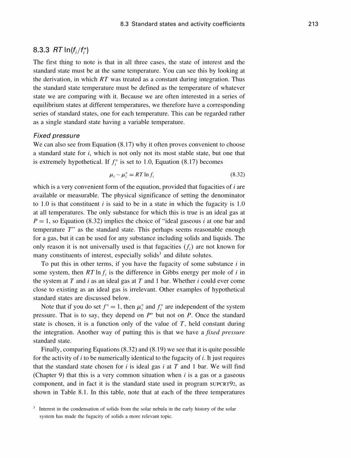
8.3 Standard states and activity coefficients 213
8.3.3 RT ln�fi/f�i �
The first thing to note is that in all three cases, the state of interest and thestandard state must be at the same temperature. You can see this by looking atthe derivation, in which RT was treated as a constant during integration. Thusthe standard state temperature must be defined as the temperature of whateverstate we are comparing with it. Because we are often interested in a series ofequilibrium states at different temperatures, we therefore have a correspondingseries of standard states, one for each temperature. This can be regarded ratheras a single standard state having a variable temperature.
Fixed pressureWe can also see from Equation (8.17) why it often proves convenient to choosea standard state for i, which is not only not its most stable state, but one thatis extremely hypothetical. If f �
i is set to 1.0, Equation (8.17) becomes
�i−��i = RT ln fi (8.32)
which is a very convenient form of the equation, provided that fugacities of i areavailable or measurable. The physical significance of setting the denominatorto 1.0 is that constituent i is said to be in a state in which the fugacity is 1.0at all temperatures. The only substance for which this is true is an ideal gas atP = 1, so Equation (8.32) implies the choice of “ideal gaseous i at one bar andtemperature T” as the standard state. This perhaps seems reasonable enoughfor a gas, but it can be used for any substance including solids and liquids. Theonly reason it is not universally used is that fugacities �fi� are not known formany constituents of interest, especially solids3 and dilute solutes.
To put this in other terms, if you have the fugacity of some substance i insome system, then RT ln fi is the difference in Gibbs energy per mole of i inthe system at T and i as an ideal gas at T and 1 bar. Whether i could ever comeclose to existing as an ideal gas is irrelevant. Other examples of hypotheticalstandard states are discussed below.
Note that if you do set f � = 1, then ��i and f
�i are independent of the system
pressure. That is to say, they depend on P� but not on P. Once the standardstate is chosen, it is a function only of the value of T , held constant duringthe integration. Another way of putting this is that we have a fixed pressurestandard state.
Finally, comparing Equations (8.32) and (8.19) we see that it is quite possiblefor the activity of i to be numerically identical to the fugacity of i. It just requiresthat the standard state chosen for i is ideal gas i at T and 1 bar. We will find(Chapter 9) that this is a very common situation when i is a gas or a gaseouscomponent, and in fact it is the standard state used in program supcrt92, asshown in Table 8.1. In this table, note that at each of the three temperatures
3 Interest in the condensation of solids from the solar nebula in the early history of the solarsystem has made the fugacity of solids a more relevant topic.
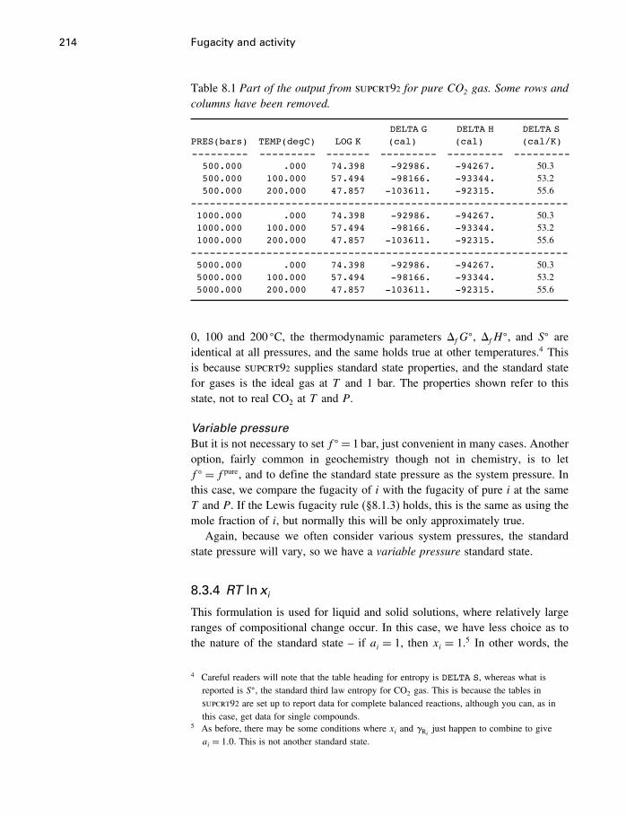
214 Fugacity and activity
Table 8.1 Part of the output from supcrt92 for pure CO2 gas. Some rows andcolumns have been removed.
DELTA G DELTA H DELTA SPRES(bars) TEMP(degC) LOG K (cal) (cal) (cal/K)--------- --------- ------- --------- --------- ---------
500.000 .000 74.398 -92986. -94267. 50�3500.000 100.000 57.494 -98166. -93344. 53�2500.000 200.000 47.857 -103611. -92315. 55�6
------------------------------------------------------------1000.000 .000 74.398 -92986. -94267. 50�31000.000 100.000 57.494 -98166. -93344. 53�21000.000 200.000 47.857 -103611. -92315. 55�6
------------------------------------------------------------5000.000 .000 74.398 -92986. -94267. 50�35000.000 100.000 57.494 -98166. -93344. 53�25000.000 200.000 47.857 -103611. -92315. 55�6
0, 100 and 200 �C, the thermodynamic parameters �fG�, �fH
�, and S� areidentical at all pressures, and the same holds true at other temperatures.4 Thisis because supcrt92 supplies standard state properties, and the standard statefor gases is the ideal gas at T and 1 bar. The properties shown refer to thisstate, not to real CO2 at T and P.
Variable pressureBut it is not necessary to set f � = 1 bar, just convenient in many cases. Anotheroption, fairly common in geochemistry though not in chemistry, is to letf � = f pure, and to define the standard state pressure as the system pressure. Inthis case, we compare the fugacity of i with the fugacity of pure i at the sameT and P. If the Lewis fugacity rule (§8.1.3) holds, this is the same as using themole fraction of i, but normally this will be only approximately true.
Again, because we often consider various system pressures, the standardstate pressure will vary, so we have a variable pressure standard state.
8.3.4 RT lnxi
This formulation is used for liquid and solid solutions, where relatively largeranges of compositional change occur. In this case, we have less choice as tothe nature of the standard state – if ai = 1, then xi = 1.5 In other words, the
4 Careful readers will note that the table heading for entropy is DELTA S, whereas what isreported is S�, the standard third law entropy for CO2 gas. This is because the tables insupcrt92 are set up to report data for complete balanced reactions, although you can, as inthis case, get data for single compounds.
5 As before, there may be some conditions where xi and Ri just happen to combine to giveai = 1�0. This is not another standard state.
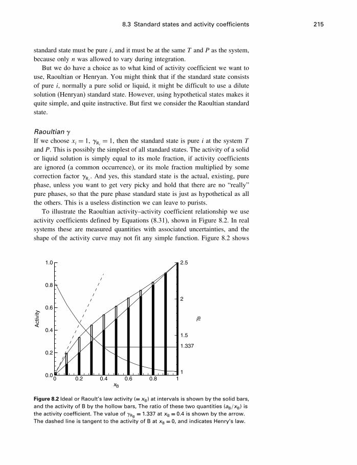
8.3 Standard states and activity coefficients 215
standard state must be pure i, and it must be at the same T and P as the system,because only n was allowed to vary during integration.
But we do have a choice as to what kind of activity coefficient we want touse, Raoultian or Henryan. You might think that if the standard state consistsof pure i, normally a pure solid or liquid, it might be difficult to use a dilutesolution (Henryan) standard state. However, using hypothetical states makes itquite simple, and quite instructive. But first we consider the Raoultian standardstate.
Raoultian �
If we choose xi = 1, Ri = 1, then the standard state is pure i at the system T
and P. This is possibly the simplest of all standard states. The activity of a solidor liquid solution is simply equal to its mole fraction, if activity coefficientsare ignored (a common occurrence), or its mole fraction multiplied by somecorrection factor Ri . And yes, this standard state is the actual, existing, purephase, unless you want to get very picky and hold that there are no “really”pure phases, so that the pure phase standard state is just as hypothetical as allthe others. This is a useless distinction we can leave to purists.
To illustrate the Raoultian activity–activity coefficient relationship we useactivity coefficients defined by Equations (8.31), shown in Figure 8.2. In realsystems these are measured quantities with associated uncertainties, and theshape of the activity curve may not fit any simple function. Figure 8.2 shows
xB
Act
ivity
γ B
0 0.2 0.4 0.6 0.8 10.0
0.2
0.4
0.6
0.8
1.0
1
1.5
2
2.5
1.337
Figure 8.2 Ideal or Raoult’s law activity (= xB) at intervals is shown by the solid bars,and the activity of B by the hollow bars, The ratio of these two quantities (aB/xB) isthe activity coefficient. The value of �RB
= 1�337 at xB = 0�4 is shown by the arrow.The dashed line is tangent to the activity of B at xB = 0, and indicates Henry’s law.
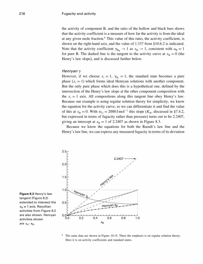
216 Fugacity and activity
the activity of component B, and the ratio of the hollow and black bars showsthat the activity coefficient is a measure of how far the activity is from the idealat any given mole fraction.6 This value of this ratio, the activity coefficient, isshown on the right-hand axis, and the value of 1.337 from §10.6.2 is indicated.Note that the activity coefficient RB
→ 1 as xB → 1, consistent with aB = 1for pure B. The dashed line is the tangent to the activity curve at xB = 0 (theHenry’s law slope), and is discussed further below.
Henryan �
However, if we choose xi = 1, Hi = 1, the standard state becomes a purephase (xi = 1) which forms ideal Henryan solutions with another component.But the only pure phase which does this is a hypothetical one, defined by theintersection of the Henry’s law slope at the other component composition withthe xi = 1 axis. All compositions along this tangent line obey Henry’s law.Because our example is using regular solution theory for simplicity, we knowthe equation for the activity curve, so we can differentiate it and find the valueof this at xB = 0. With wG = 2000 Jmol−1 this slope (KH, discussed in §7.4.2,but expressed in terms of fugacity rather than pressure) turns out to be 2.2407,giving an intercept at xB = 1 of 2.2407 as shown in Figure 8.3.
Because we know the equations for both the Raoult’s law line and theHenry’s law line, we can express any measured fugacity in terms of its deviation
Figure 8.3 Henry’s lawtangent (Figure 8.2)extended to intersect thexB = 1 axis. Raoultianactivities from Figure 8.2are also shown. Henryanactivities shownare �H ·xB. xB
0.0 0.2 0.4 0.6 0.8 1.00.0
0.5
1.0
1.5
2.0
2.5
Henry’s l
aw
Henryan aB
Henryan γB
2.2407
6 The same data are shown in Figure 10.15. There the emphasis is on regular solution theory.Here it is on activity coefficients and standard states.
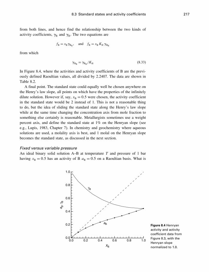
8.3 Standard states and activity coefficients 217
from both lines, and hence find the relationship between the two kinds ofactivity coefficients, R and H. The two equations are
fB = xBRB� and fB = xBKH HB
from which
HB= RB
/KH (8.33)
In Figure 8.4, where the activities and activity coefficients of B are the previ-ously defined Raoultian values, all divided by 2.2407. The data are shown inTable 8.2.
A final point. The standard state could equally well be chosen anywhere onthe Henry’s law slope, all points on which have the properties of the infinitelydilute solution. However if, say, xB = 0�5 were chosen, the activity coefficientin the standard state would be 2 instead of 1. This is not a reasonable thingto do, but the idea of sliding the standard state along the Henry’s law slopewhile at the same time changing the concentration axis from mole fraction tosomething else certainly is reasonable. Metallurgists sometimes use a weightpercent axis, and define the standard state at 1% on the Henryan slope (seee.g., Lupis, 1983, Chapter 7). In chemistry and geochemistry where aqueoussolutions are used, a molality axis is best, and 1 molal on the Henryan slopebecomes the standard state, as discussed in the next section.
Fixed versus variable pressureAn ideal binary solid solution A–B at temperature T and pressure of 1 barhaving xB = 0�5 has an activity of B aB = 0�5 on a Raoultian basis. What is
XB
aB
γB
0.0 0.2 0.4 0.6 0.8 1.00.0
0.2
0.4
0.6
0.8
1.0
a B, γ
B
Figure 8.4 Henryanactivity and activitycoefficient data fromFigure 8.3, with theHenryan slopenormalized to 1.0.
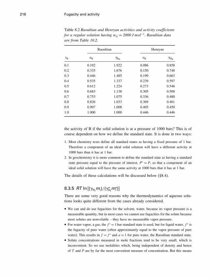
218 Fugacity and activity
Table 8.2 Raoultian and Henryan activities and activity coefficientsfor a regular solution having wG = 2000 J mol−1. Raoultian dataare from Table 10.2.
Raoultian Henryan
xB aB RBaB HB
0.1 0.192 1.922 0.086 0.858
0.2 0.335 1.676 0.150 0.748
0.3 0.446 1.485 0.199 0.663
0.4 0.535 1.337 0.239 0.597
0.5 0.612 1.224 0.273 0.546
0.6 0.683 1.138 0.305 0.508
0.7 0.753 1.075 0.336 0.480
0.8 0.826 1.033 0.369 0.461
0.9 0.907 1.008 0.405 0.450
1.0 1.000 1.000 0.446 0.446
the activity of B if the solid solution is at a pressure of 1000 bars? This is ofcourse dependent on how we define the standard state. It is done in two ways:
1. Most chemistry texts define all standard states as having a fixed pressure of 1 bar.
Therefore a component of an ideal solid solution will have a different activity at
1000 bars than it has at 1 bar.
2. In geochemistry it is more common to define the standard state as having a standard
state pressure equal to the pressure of interest, P� = P, so that a component of an
ideal solid solution will have the same activity at 1000 bars that it has at 1 bar.
The details of these calculations will be discussed below (§8.4).
8.3.5 RT ln ��Himi �/��
�Him�
i �
There are some very good reasons why the thermodynamics of aqueous solu-tions looks quite different from the cases already considered.
• We can and do use fugacities for the solvent, water, because its vapor pressure is a
measurable quantity, but in most cases we cannot use fugacities for the solute because
most solutes are nonvolatile – they have no measurable vapor pressure.• For water vapor, a gas, the f � = 1 bar standard state is used, but for liquid water, f � isthe fugacity of pure water (often approximately equal to the vapor pressure of pure
water). This results in f = f � and a= 1 for pure water, the Raoultian standard state.• Solute concentrations measured in mole fractions tend to be very small, which is
inconvenient. So we use molalities which, being independent of density and hence
of T and P are by far the most convenient measure of concentration. But this means
8.3 Standard states and activity coefficients 219
that we cannot use the pure solute as a standard state, because m becomes infinite
for the pure solute. We must use different standard states for the solvent and solute,
a situation often called “unsymmetrical,” but which in itself causes no problems.
• We can use a Raoultian standard state (pure water) for the solvent, but its deviation
from ideal behavior, whether based on a mole fraction or a molality scale, is often
converted to the osmotic coefficient �, which does not actually have a standard state.
It is an absolute system property.
We look first at the solute and then at the solvent.
8.3.6 Activity coefficients of solutes
Activities of the solute, whether electrolyte or nonelectrolyte, use molalitiesand the ��
Him�i � standard state. We must now examine what this means.
We want to use the Henryan standard state, which is a state in which thesolute exhibits dilute solution behavior. That is, no matter what the actualconcentration, the solute behaves as if there is absolutely no solute–soluteinteractions – each solute molecule thinks it is alone in the solvent. It is astate which obey’s Henry’s law, which at real concentrations is obviously ahypothetical state, and it lies anywhere on the Henry’s law tangent. In §8.3.4we saw that we could choose a point on this tangent having xi = 1, or we couldchoose any other point. What the other points on this slope mean depends onwhat concentration scale we are using – if we use a weight percent scale wecan choose a weight percent standard state, and if we use a molality scale wecan choose a molal standard state.
Although theoretically we could choose any value for m�, any choice exceptm� = 1 would introduce complications, and of course we want �
H = 1 so thatthe standard state lies on the tangent and refers to properties at infinite dilution.This leads to the adoption of the “hypothetical ideal one molal” standard statefor aqueous solutes. If in Figure 8.4 we change the concentration scale tomolality, and focus on the lower left corner of the diagram, we have Figure 8.5.We have assumed that B is a nonelectrolyte with � = 1 such as sucrose oroxygen, and the conversion is
mB = 55�51 ·xB1−xB
In this case, in which we have continued our example of a regular solutionhaving wG = 2000 Jmol−1, the solution does not deviate from the ideal verygreatly until molalities well above 1m. Activity coefficients based on molefractions and molalities are shown in Table 8.3. The reason for two slightlydifferent values of H, Hx and Hm, is that molality is not exactly proportionalto mole fraction except in the limit of infinite dilution, so that a Henryan tangent
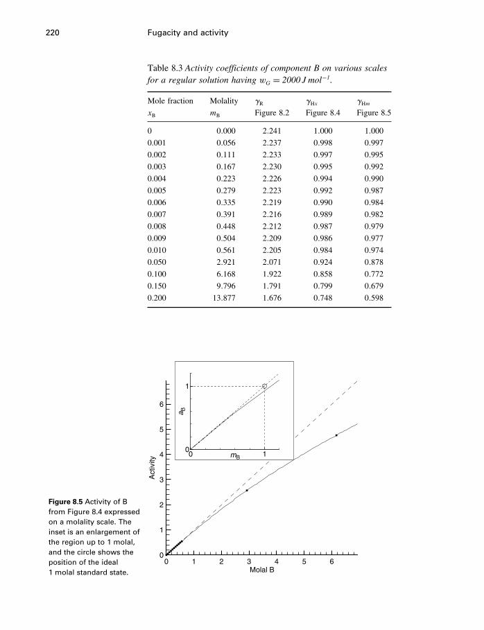
220 Fugacity and activity
Table 8.3 Activity coefficients of component B on various scalesfor a regular solution having wG = 2000 J mol−1.
Mole fraction Molality R Hx HmxB mB Figure 8.2 Figure 8.4 Figure 8.5
0 0�000 2�241 1�000 1�000
0.001 0�056 2�237 0�998 0�997
0.002 0�111 2�233 0�997 0�995
0.003 0�167 2�230 0�995 0�992
0.004 0�223 2�226 0�994 0�990
0.005 0�279 2�223 0�992 0�987
0.006 0�335 2�219 0�990 0�984
0.007 0�391 2�216 0�989 0�982
0.008 0�448 2�212 0�987 0�979
0.009 0�504 2�209 0�986 0�977
0.010 0�561 2�205 0�984 0�974
0.050 2�921 2�071 0�924 0�878
0.100 6�168 1�922 0�858 0�772
0.150 9�796 1�791 0�799 0�679
0.200 13�877 1�676 0�748 0�598
Molal B
Act
ivity
0 1 2 3 4 5 60
1
2
3
4
5
6
mB
a B
0 10
1
Figure 8.5 Activity of Bfrom Figure 8.4 expressedon a molality scale. Theinset is an enlargement ofthe region up to 1 molal,and the circle shows theposition of the ideal1 molal standard state.
8.3 Standard states and activity coefficients 221
on a mole fraction diagram will appear to be slightly curved on a molalitydiagram. The correction factor for activity coefficients is
ln �Hx�= ln �Hm�+ ln �1+0�018 0154m�
and, as you can see, it is insignificant until quite large molalities are reached.
In this section the magnitude of our activity coefficients has been fixedby our choice of a regular solution model. We did this so as to producerealistic numbers, and to concentrate on the meanings of activity coefficientsand standard states. In most situations, however, activity coefficients are eithermeasured in a laboratory situation, or they are calculated on a theoretical basisto serve as correction factors to some known concentrations in modeling areal solution or equilibrium. They will not always fit a regular solution model,although the results of Aranovich and Newton are interesting in this regard,as mentioned above. The calculation of activity coefficients from electrostaticconsiderations will be discussed in Chapter 15.
8.3.7 Osmotic coefficients
In aqueous solutions the activity of the pure solvent, measured as f/f �, is 1.0.In dilute solutions, the focus of a great deal of solution chemistry, the activityremains very close to 1.0, so its accurate expression requires several significantfigures. The example given by Robinson and Stokes (1959), a classic reference,is a 2 molal KCl solution, which has a water mole fraction of 0.9328 and awater activity of 0.9364. Its activity coefficient is therefore 1.004, a figure“which fails to emphasize the departure from ideality indicated by the activitycoefficient of the solute,” which is 0.614. To overcome this problem use ofthe osmotic coefficient has become standard practice, even though its slopechanges sign at concentrations above about 1 molal, as shown in Figure 8.6a.The same pattern, this time for NaCl solutions, becomes more subdued athigher temperatures and pressures (Figure 8.6b). A less complicated pattern isshown by many nonelectrolytes such as sucrose, shown in Figure 8.7.
Osmotic pressureThe osmotic coefficient has its origin, as you might suspect, through its con-nection with osmotic pressures. The chemical potential of water in an aqueoussolution is inherently less than that of the pure solvent, as you can see from�1 −��
1 = RT ln x1. If this solution is separated from the pure solvent by amembrane permeable only to the solvent, pure solvent will pass through themembrane into the solution in an attempt to remove this difference. If the
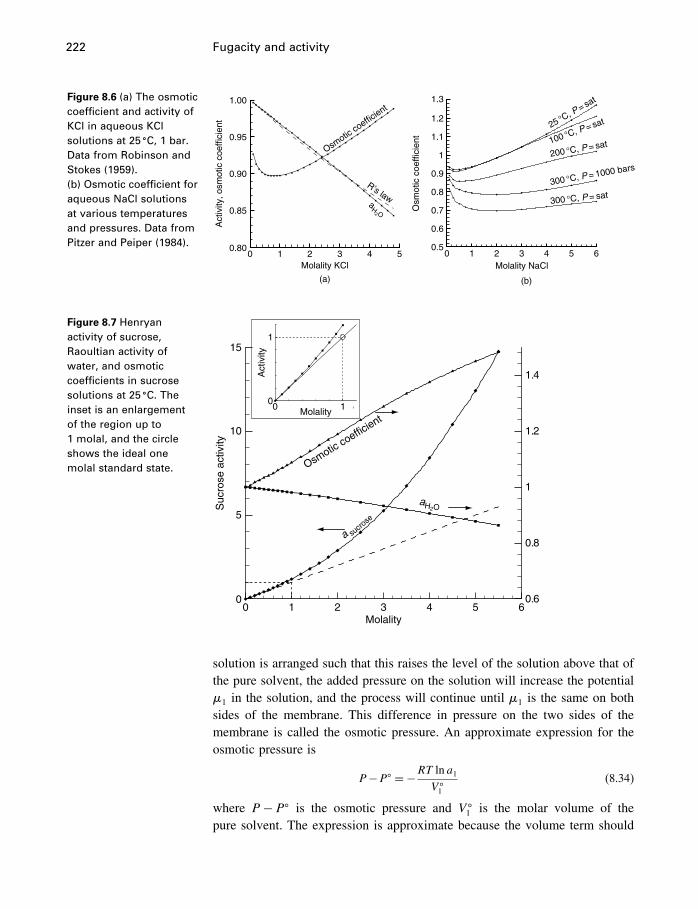
222 Fugacity and activity
Figure 8.6 (a) The osmoticcoefficient and activity ofKCl in aqueous KClsolutions at 25 �C, 1 bar.Data from Robinson andStokes (1959).(b) Osmotic coefficient foraqueous NaCl solutionsat various temperaturesand pressures. Data fromPitzer and Peiper (1984).
Molality KCl
Act
ivity
, osm
otic
coe
ffici
ent
0.80
0.85
0.90
0.95
1.00
0 1 2 3 4 5
R’s lawaH
2O
Osmotic
coeffic
ient
(a)
Molality NaCl
Osm
otic
coe
ffici
ent
0.5
0.6
0.7
0.8
0.9
1
1.1
1.2
1.3
300 °C, P = 1000 bars
0 1 2 3 4 5 6
25 °C, P = sat
100 °C, P = sat
200 °C, P = sat
300 °C, P = sat
(b)
Figure 8.7 Henryanactivity of sucrose,Raoultian activity ofwater, and osmoticcoefficients in sucrosesolutions at 25 �C. Theinset is an enlargementof the region up to1 molal, and the circleshows the ideal onemolal standard state.
Molality
Suc
rose
act
ivity
0 1 2 3 4 5 60
5
10
15
0.6
0.8
1
1.2
1.4
Osmotic coefficient
aH2O
a sucro
se
Molality
Act
ivity
0 10
1
solution is arranged such that this raises the level of the solution above that ofthe pure solvent, the added pressure on the solution will increase the potential�1 in the solution, and the process will continue until �1 is the same on bothsides of the membrane. This difference in pressure on the two sides of themembrane is called the osmotic pressure. An approximate expression for theosmotic pressure is
P−P� = −RT lna1V �1
(8.34)
where P − P� is the osmotic pressure and V �1 is the molar volume of the
pure solvent. The expression is approximate because the volume term should
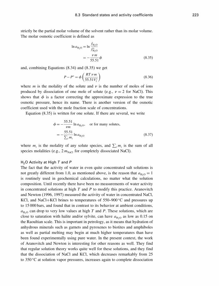
8.3 Standard states and activity coefficients 223
strictly be the partial molar volume of the solvent rather than its molar volume.The molar osmotic coefficient is defined as
lnaH2O= ln
fH2O
f �H2O
=− �m
55�51� (8.35)
and, combining Equations (8.34) and (8.35) we get
P−P� = �(RT �m
55�51V �1
)(8.36)
where m is the molality of the solute and � is the number of moles of ionsproduced by dissociation of one mole of solute (e.g., � = 2 for NaCl). Thisshows that � is a factor correcting the approximate expression to the trueosmotic pressure, hence its name. There is another version of the osmoticcoefficient used with the mole fraction scale of concentrations.
Equation (8.35) is written for one solute. If there are several, we write
�=−55�51�m
lnaH2O� or for many solutes,
=− 55�51∑i mi
lnaH2O(8.37)
where mi is the molality of any solute species, and∑i mi is the sum of all
species molalities (e.g., 2mNaCl for completely dissociated NaCl).
H2O Activity at High T and P
The fact that the activity of water in even quite concentrated salt solutions isnot greatly different from 1.0, as mentioned above, is the reason that aH2O
= 1is routinely used in geochemical calculations, no matter what the solutioncomposition. Until recently there have been no measurements of water activityin concentrated solutions at high T and P to modify this practice. Aranovitchand Newton (1996, 1997) measured the activity of water in concentrated NaCl,KCl, and NaCl+KCl brines to temperatures of 550–900 �C and pressures upto 15 000 bars, and found that in contrast to its behavior at ambient conditions,aH2O
can drop to very low values at high T and P. These solutions, which areclose to saturation with halite and/or sylvite, can have aH2O
as low as 0.15 onthe Raoultian scale. This is important in petrology, as it means that hydration ofanhydrous minerals such as garnets and pyroxenes to biotites and amphibolesas well as partial melting may begin at much higher temperatures than havebeen found experimentally using pure water. In the present context, the workof Aranovitch and Newton is interesting for other reasons as well. They findthat regular solution theory works quite well for these solutions, and they findthat the dissociation of NaCl and KCl, which decreases remarkably from 25to 350 �C at solution vapor pressures, increases again to complete dissociation
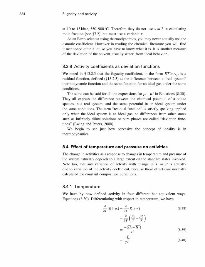
224 Fugacity and activity
at 10 to 15 kbar, 550–900 �C. Therefore they do not use � = 2 in calculatingmole fraction (see §7.2), but must use a variable �.
As an Earth scientist using thermodynamics, you may never actually use theosmotic coefficient. However in reading the chemical literature you will findit mentioned quite a lot, so you have to know what it is. It is another measureof the deviation of the solvent, usually water, from ideal behavior.
8.3.8 Activity coefficients as deviation functions
We noted in §13.2.3 that the fugacity coefficient, in the form RT lnf , is aresidual function, defined (§13.2.3) as the difference between a “real system”thermodynamic function and the same function for an ideal gas under the sameconditions.
The same can be said for all the expressions for �−�� in Equations (8.30).They all express the difference between the chemical potential of a solutespecies in a real system, and the same potential in an ideal system underthe same conditions. The term “residual function” is strictly speaking appliedonly when the ideal system is an ideal gas, so differences from other statessuch as infinitely dilute solutions or pure phases are called “deviation func-tions” (Ewing and Peters, 2000).
We begin to see just how pervasive the concept of ideality is inthermodynamics.
8.4 Effect of temperature and pressure on activities
The change in activities as a response to changes in temperature and pressure ofthe system naturally depends to a large extent on the standard states involved.Note too, that any variation of activity with change in T or P is actuallydue to variation of the activity coefficient, because these effects are normallycalculated for constant composition conditions.
8.4.1 Temperature
We have by now defined activity in four different but equivalent ways,Equations (8.30). Differentiating with respect to temperature, we have
�
�T�R lnai�=
�
�T�R lni� (8.38)
= �
�T
(�iT
− ��i
T
)
= −�Hi−H�i �
T 2(8.39)
= −LiT 2
(8.40)
8.4 Effect of temperature and pressure on activities 225
where i may be f , R, or H. Thus the temperature derivative of the activityis a simple function of the relative partial molar enthalpy, Li, which wasdiscussed in §9.3.3. The numerical value of Li of course depends on the form ofactivity being used, because this determines the value of H
�i . For standard states
based on Raoult’s law, that is, where the standard state is the pure substancei at T and P, H
�i is the same as H�
i , the molar enthalpy of the substance (anunknown quantity, but as usual it appears in a difference term, so we don’tneed to know its absolute value).
For the ideal gaseous standard state, H�i is evidently the molar enthalpy
of an ideal gas. For standard states based on Henry’s law, where H → 1 asx or m→ 0, H
�i is the partial molar enthalpy of the solute in the hypothetical
pure substance having H = 1 or the hypothetical ideal one molal solutionrespectively. Substances in these strange states have partial molar enthalpies(and volumes) equal to that at infinite dilution, hence providing a method ofmeasurement. This can be seen by considering Equations (8.38) and (8.39),which show that H
�i becomes equal to Hi when i is 1.0. Therefore for Henryan
standard states where i → 1 as xi or m→ 0, H�i must be the partial molar
enthalpy of i at infinite dilution, and for Raoultian standard states where i→ 1as xi → 1, H
�i must be the partial molar enthalpy (the molar enthalpy) of pure i
(confirming what we stated by simple inspection, above).Note that in the case of multicomponent solutions infinite dilution means
infinite dilution of all components, not just of component i. Thus the Henryanstandard states, which seem so unattainable, are actually convenient becausesome of their properties are the same as those of the infinitely dilute solu-tion, and these are obtainable by extrapolation from measurements at finiteconcentration.
8.4.2 Pressure
In considering the effect of pressure on activity, we must recall that the standardstate pressure (P�� is not always the same as the system pressure �P�, so thatthe differentiation with respect to pressure is not always completely analogousto differentiation with respect to temperature. The argument here is very similarto that in §6.3.2.
First of all, for variable pressure standard states, those that do have P� = P,we have
�
�P�RT lnai�=
�
�P�RT lni�
= �
�P��i−��
i �
= V i−V �i
where i may be f , R, or H, and V�i is either the molar volume of pure i or
the partial molar volume of i at infinite dilution, depending on the standard state
226 Fugacity and activity
used (see above). Integration of this expression requires a knowledge of thevariation of the relative partial molar volume V i−V �
i with pressure for whichthere is no general expression. There is also no special symbol for V i−V �
i asthere is for Hi−H�
i .However for the fixed pressure standard states,
�
�P���
i �= 0 (8.41)
because changing P does not change the pressure on the standard state �P��.Therefore
�
�P�R lnai�= V i
A case of particular interest to us is the activity of solids, for which in manycases the assumption that V i is unaffected by pressure (solid i is incompressible)is reasonable. If V i is a constant, then∫ P2
P1
d lnai =1RT
∫ P2
P1
V idP
ln�ai�P2 − ln�ai�P1 = V i�P2−P1�/RT
Furthermore, if P1 = 1 bar and the standard state of i is pure i at T and onebar, then pure i at P1 has an activity of 1, and
ln�ai�P2 = ln�ai�P = V i�P−1�/RT
or for pure solids
ln�ai�P = Vi�P−1�/RT (8.42)
This permits calculation of the activity of a pure mineral at any pressure,relative to the same mineral at one bar.
For example, consider calcite and aragonite at equilibrium at 3737 bars and25 �C, from our example in Chapter 6. The molar volumes of calcite and arag-onite are taken from Appendix B (or Table 6.1), so for calcite Equation (8.42)gives
lnacalcite�P=3737 = 3�6934 · �3737−1�/�8�31451×298�15�
= 5�566
so
acalcite�P=3737 = 261
and the activity of aragonite is
lnaaragonite�P=3737 = 3�4150 · �3737−1�/�8�31451×298�15�
= 5�147
8.5 Activities and standard states: an overall view 227
so
aaragonite�P=3737 = 172
Thus CaCO3 in the form of calcite and aragonite at 3737 bars, althoughhaving the same chemical potential, has two different activities because thereare two different standard states. Recalling that activity is the ratio fi/f
�i , we
see too that the physical meaning of an activity of calcite of 261 is that thefugacity (which ≈ vapor pressure) of calcite is increased by a factor of 261when it is squeezed from 1 bar to 3737 bars. We know this without knowingeither f at 3737 bars or f � at one bar for calcite.
8.5 Activities and standard states: an overall view
We have now said everything necessary about activities and standard states, butthe overall effect for the newcomer is often one of confusion at this stage. Totry to draw the various threads together we consider in Figure 8.8 a hypotheticalthree-phase equilibrium at temperature T and pressure P. A solid crystallinesolution of B in A is in contact with an aqueous solution of A(aq) and B(aq),which is in turn in contact with a vapor phase containing A(v) and B(v) inaddition to water vapor. We can suppose the dissolution of (A,B)(s) to bestoichiometric so that the ratio of A to B is the same in all three phases, but thisis irrelevant to our development as we consider only component A. Let’s saythat for a solid solution composition of xA = 0�5, xB = 0�5, the concentrationof A(aq) at equilibrium (mA� is 10
−2 molal, and the fugacity of A in the vapor(fA� is 10
−5 bars. Assuming activity coefficients in the solid and liquid phasesto be 1.0, the activity of A in the solid solution (using a standard state of purecrystalline A at T and P� is 0.5, the activity of A in the aqueous solution(using a standard state of the hypothetical ideal one molal solution of A atT and P� is 10−2, and the activity of A in the vapor (using a standard stateof pure ideal gaseous A at T and one bar) is 10−5. Because the system isat equilibrium, the chemical potential of A (�A� is the same in each of thethree phases, but because the three standard states are different, the standardchemical potential of A ���
A� is different for the three phases. The difference(�A−��
A� is calculable from the equations we have just derived. Thus, lettingT = 25 �C�
��A−��A�solid = RT ln xA
= 8�31451×298�15× ln �0�5�
=−1�72kJmol−1
��A−��A�aq = RT lnmA
= 8�31451×298�15× ln�10−2�
=−11�4kJmol−1
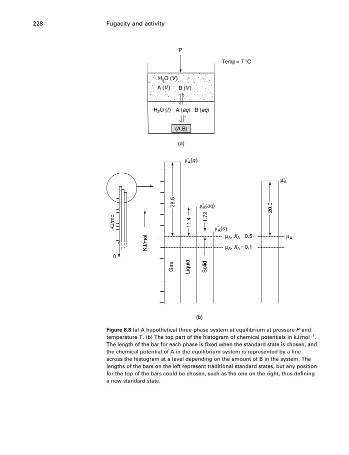
228 Fugacity and activity
(b)
KJ/
mol
KJ/
mol
0
µA(g )
µA(aq)
µA(s )
28.5
11.4 1.
72
Gas
Liqu
id
Sol
id
µA, XA = 0.5
µA, XA = 0.1
µA
µA
20.0
°
°
°
°
(a)
Temp = T °C
H2O (V )
A (V ) B (V )
H2O (l ) A (aq) B (aq)
(A,B)
P
Figure 8.8 (a) A hypothetical three-phase system at equilibrium at pressure P andtemperature T . (b) The top part of the histogram of chemical potentials in kJmol−1.The length of the bar for each phase is fixed when the standard state is chosen, andthe chemical potential of A in the equilibrium system is represented by a lineacross the histogram at a level depending on the amount of B in the system. Thelengths of the bars on the left represent traditional standard states, but any positionfor the top of the bars could be chosen, such as the one on the right, thus defininga new standard state.
8.5 Activities and standard states: an overall view 229
��A−��A�gas = RT ln fA
= 8�31451×298�15× ln�10−5�
=−28�5kJmol−1
It is instructive to consider these differences on a histogram (Figure 8.8)in which the ordinate is a scale of kJmol−1, on which we plot the absolutechemical potentials of A. These absolute potentials may be very large, so welook at only the tops of the bars in the histogram, and we unfortunately don’tknow the values of the absolute potentials individually, so we can’t put anabsolute scale on the ordinate. But we can plot the relative positions of thetops of the bars, and the position of the equilibrium chemical potential of A inthe system.
If we now consider systems having more and more B in the solid solu-tion (and hence in the other two phases), but always at equilibrium, the his-togram bars stay where they are (because we are not changing standard states)but the level of the (absolute) chemical potential of A is lowered, increas-ing the distance between the top of the histogram bar for each phase andthe level of �A, that is, increasing the (negative) value of ��A −��
A� as theactivity of A is lowered.
This diagram is worth careful thought. It illustrates several things that areuseful in understanding activities, chemical potentials, and standard states,such as the absolute nature of chemical potentials and the necessity of usingdifferences, the equality of chemical potentials in each phase, and the arbitrarynature of the standard state.
This is all very nice, but wouldn’t it be a lot simpler to have the same activityin every phase, just as we have the same chemical potential in every phase? Thisis worth some thought too. Having the same activity in each phase means havingthe same value of �−�� in each phase, and presumably we could choose what-ever value we like for this. If we chose this to be −20kJmol−1, the histogramfor every phase would look like that shown in Figure 8.8. Then because the threestandard states have the same value of ��, they could all coexist at equilibrium(if they could exist at all). However, arbitrarily choosing ai means arbitrarilychoosing f �
i and m�i , and this results in some standard states that are even more
weird than the traditional ones. For example, if �−�� = −20kJmol−1, thenai = 10−3�50, and if mi = 10−5 and mi/m
�i = 10−3�5, then m�
i = 101�5 or 31.9. Sothe standard state becomes a hypothetical ideal 31.9 molal solution.
So probably it is better to stick to having different standard states anddifferent activities in each phase.
8.5.1 Changing standard states
Another way to think about standard states is to consider how to change fromone to another. For example, let’s say we have a real system consisting of a
230 Fugacity and activity
gas in contact with a liquid. Methane in the gas has a measured partial pressureof 0.01 bar, which we take to be its fugacity, and we want to calculate howmuch methane is dissolved in the water. In the gas phase, fCH4
= 0�01bar, andusing a standard state of ideal methane gas at 1 bar (f �
CH4= 1�0 bar), we have
an activity of methane of 0.01 (aCH4= 0�01). The relevant reaction is
CH4�g�= CH4�aq�
and getting numbers from the tables we have
�rG� = �fG
�CH4�aq�
−�fG�CH4�g�
=−34 451− �−50 720�
= 16 269 Jmol−1
This means that, because the elements all cancel out (§3.5),
G�CH4�aq�
−G�CH4�g�
= 16 269 Jmol−1
where G�CH4�aq�
is the absolute G of methane in an ideal 1 molal solution, andG�
CH4�g�is the absolute G of methane as an ideal gas at 1 bar. Then
logK =−�rG�/�2�30259RT�
=−16 269/�2�30259×8�31451×298�15�
=−2�850
where
K = aCH4�aq�
aCH4�g�
Therefore if aCH4�g�= 0�01, then
10−2�850 = aCH4�aq�
0�01
and
aCH4�aq�= 0�01×10−2�850
= 10−4�850
So the calculated activity of dissolved methane is 10−4�85. With a standard stateof ideal 1 molal methane, this means mCH4
CH4= 10−4�85, and on the reasonable
assumption that CH4= 1�0, then mCH4
= 10−4�85. So in spite of the fact that twodifferent standard states are used for the same component in the same reaction,we arrive at a useful answer. This is because the standard states used do not
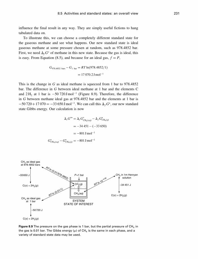
8.5 Activities and standard states: an overall view 231
influence the final result in any way. They are simply useful fictions to hangtabulated data on.
To illustrate this, we can choose a completely different standard state forthe gaseous methane and see what happens. Our new standard state is idealgaseous methane at some pressure chosen at random, such as 978.4852 bar.First, we need �fG
� of methane in this new state. Because the gas is ideal, thisis easy. From Equation (8.5), and because for an ideal gas, f = P,
G978�4852 bars−G1 bar = RT ln�978�4852/1�
= 17 070�2 Jmol−1
This is the change in G as ideal methane is squeezed from 1 bar to 978.4852bar. The difference in G between ideal methane at 1 bar and the elements Cand 2H2 at 1 bar is −50 720 Jmol−1 (Figure 8.9). Therefore, the differencein G between methane ideal gas at 978.4852 bar and the elements at 1 bar is−50 720+17 070=−33 650 Jmol−1. We can call this �fG
�, our new standardstate Gibbs energy. Our calculation is now
�rG�� = �fG
�CH4�aq�
−�fG�CH4�g�
=−34 451− �−33 650�
=−801 Jmol−1
G�CH4�aq�
−G�CH4�g�=−801 Jmol−1
CH4 as ideal gasat 978.4852 bars
CH4 as ideal gasat 1 bar
–33650 J
–50720 J
C(s ) + 2H2(g )
C(s ) + 2H2(g )
C(s ) + 2H2(g )
RT ln (0.01/978.4852)
RT ln (0.01/1)
RT ln 10–4.85
SYSTEMSTATE OF INTEREST
P =1 bar
CH4(g)
CH4(aq)
CH4 in 1m Henryansolution
–34 451 J
Figure 8.9 The pressure on the gas phase is 1 bar, but the partial pressure of CH4 inthe gas is 0.01 bar. The Gibbs energy (�) of CH4 is the same in each phase, and avariety of standard state data may be used.
232 Fugacity and activity
Then
logK =−�rG��/�2�30259RT�
= 801/�2�30259×8�31451×298�15�
= 0�140
or
K = aCH4�aq�
aCH4�g�
= 100�140
= 1�38
Now aCH4�g�is no longer 0.01. Because of the change of standard state,
aCH4�g�= fCH4�g�
f �CH4�g�
= 0�01978�4852
= 10−4�99
and so, solving for aCH4�aq�with our new K,
aCH4�aq�
aCH4�g�
= 1�38
aCH4�aq�= 1�38×aCH4�g�
= 1�38×10−4�99
= 10−4�85
as before. So using any arbitrary standard state makes no difference at all. If youfollow the calculations closely, you will see that the properties of the standardstate cannot affect the results. They are a convenient repository for tabulateddata derived from experimental work. As shown in Figure 8.9, all paths fromthe elements to the equilibrium state must give the same total change in G,becauseG of all products and reactants is fixed in both states. The standard stateis merely a repository somewhere along the elements→equilibrium state path.
Units againA reminder:
• Activities and activity coefficients (a, ) have no units, but fugacity (f ) does.• Activities have standard states, but fugacities do not.
8.6 Summary 233
8.6 Summary
It would be hard to overemphasize the importance of the concepts of fugacityand activity and their relationship to the chemical potential, at least in chemi-cal thermodynamics. In thermodynamics for engineers or physicists, chemicalreactions play a smaller role, but for anyone interested in processes involvingchemical changes, this is a central topic. That is because the fugacity and activ-ity are the parameters which relate the composition of a system to its Gibbsenergy; how changes in phase compositions change the Gibbs energy of the sys-tem, and so determine the equilibrium phase compositions at a given T and P.
Fugacity and activity are basically compositional terms. In ideal solutionsthey are not necessary; pressure and various composition terms can be directlylinked to the Gibbs energy. Real solutions have a variety of intermolecularforces, so that ideal solution models need correction factors. These correctionscan be made either to the composition terms (fugacity and activity coefficients)or to the thermodynamic potentials (excess functions), and efforts to modelthese correction factors in mathematical terms have always been, and likelyalways will be, an important research field.
Because there are three main kinds of solutions and there are several com-monly used methods of expressing concentrations, activity can take on severaldifferent forms requiring different kinds of correction factors, and becauseGibbs energy is always a difference in energy between two states, there areseveral different standard or reference states in common use. This all adds upto possible confusion, and although it is possible to learn how things are doneand to follow the rules, it is of course much better to understand the reasonsfor why things are done this way.
9The equilibrium constant
9.1 Reactions in solution
Reactions involving dissolved compounds are different in an important wayfrom reactions involving only pure compounds, such as pure solids. To seewhy, consider two reactions, one between pure compounds and one betweendissolved substances.
The first is a reaction in which all products and reactants are pure substances,the kind of reaction we have been considering up to now. It is
NaAlSiO4�s�+2SiO2�s�= NaAlSi3O8�s� (9.1)
The second is a reaction in which all products and reactants are dissolved inwater and are capable of changing their concentration:
H2CO3�aq�= HCO−3 �aq�+H+�aq� (9.2)
The temperature and pressure are normal, 298.15K and 1 bar. As usual, wewant to know which way each reaction will go. Reaction (9.1) presents no prob-lem. We look up the values of �fG
� for each compound, and calculate�rG�:
�rG� = �fG
�NaAlSi3O8
−�fG�NaAlSiO4
−2�fG�SiO2
= −3711�5− �−1978�1�−2�−856�64�
= −20�12kJmol−1
We see that the reaction as written is spontaneous; NaAlSiO4 (nepheline) andSiO2 (quartz) at 1 bar pressure should react together to form NaAlSi3O8 (albite).If the reaction does proceed (thermodynamics doesn’t tell us whether it will ornot, only that the energy gradient favors it), then nepheline and quartz get usedup during the reaction. However, while being used up, they do not change theirGibbs energies. The reaction should actually proceed as long as any reactantsare left. When either the nepheline or the quartz is used up completely, thereaction must stop. This reaction can be represented graphically as in Figure 9.1.Here we use bars to represent the magnitude of the combined Gibbs energyof the products and of the reactants. The difference in the height of the bars
234
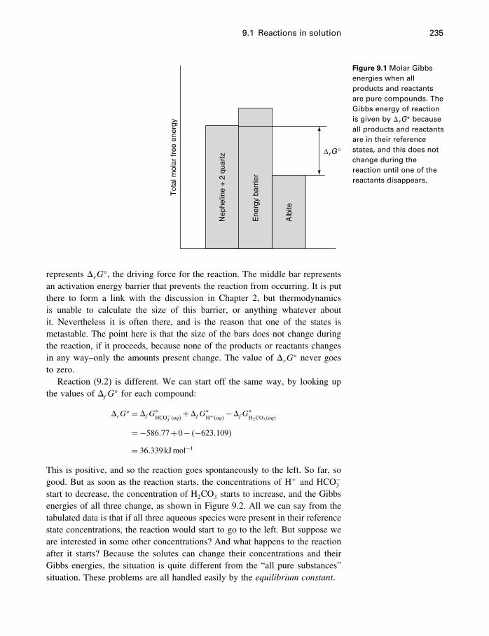
9.1 Reactions in solution 235
Nep
helin
e +
2 q
uart
z
Tot
al m
olar
free
ene
rgy
Ene
rgy
barr
ier
Alb
ite
∆rG °
Figure 9.1 Molar Gibbsenergies when allproducts and reactantsare pure compounds. TheGibbs energy of reactionis given by �rG
� becauseall products and reactantsare in their referencestates, and this does notchange during thereaction until one of thereactants disappears.
represents �rG�, the driving force for the reaction. The middle bar represents
an activation energy barrier that prevents the reaction from occurring. It is putthere to form a link with the discussion in Chapter 2, but thermodynamicsis unable to calculate the size of this barrier, or anything whatever aboutit. Nevertheless it is often there, and is the reason that one of the states ismetastable. The point here is that the size of the bars does not change duringthe reaction, if it proceeds, because none of the products or reactants changesin any way–only the amounts present change. The value of �rG
� never goesto zero.
Reaction (9.2) is different. We can start off the same way, by looking upthe values of �fG
� for each compound:
�rG� = �fG
�HCO−
3 �aq�+�fG
�H+�aq�−�fG
�H2CO3�aq�
=−586�77+0− �−623�109�
= 36�339kJmol−1
This is positive, and so the reaction goes spontaneously to the left. So far, sogood. But as soon as the reaction starts, the concentrations of H+ and HCO−
3
start to decrease, the concentration of H2CO3 starts to increase, and the Gibbsenergies of all three change, as shown in Figure 9.2. All we can say from thetabulated data is that if all three aqueous species were present in their referencestate concentrations, the reaction would start to go to the left. But suppose weare interested in some other concentrations? And what happens to the reactionafter it starts? Because the solutes can change their concentrations and theirGibbs energies, the situation is quite different from the “all pure substances”situation. These problems are all handled easily by the equilibrium constant.
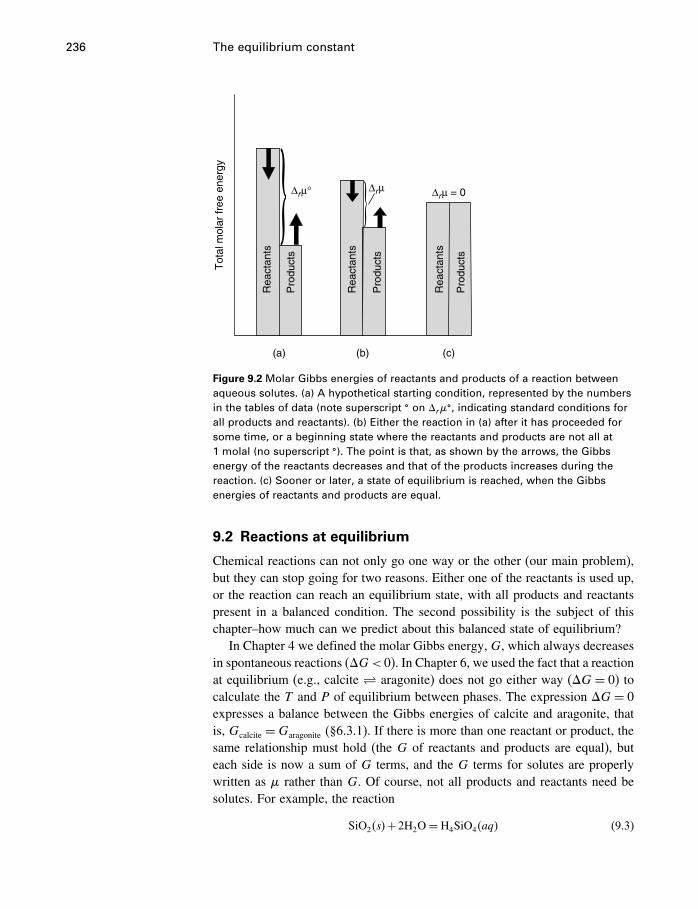
236 The equilibrium constant
(a) (b) (c)
Tot
al m
olar
free
ene
rgy
Rea
ctan
ts
Rea
ctan
ts
Rea
ctan
ts
Pro
duct
s
Pro
duct
s
Pro
duct
s
∆rµ = 0∆rµ∆rµ°
Figure 9.2 Molar Gibbs energies of reactants and products of a reaction betweenaqueous solutes. (a) A hypothetical starting condition, represented by the numbersin the tables of data (note superscript � on �r�
�, indicating standard conditions forall products and reactants). (b) Either the reaction in (a) after it has proceeded forsome time, or a beginning state where the reactants and products are not all at1 molal (no superscript �). The point is that, as shown by the arrows, the Gibbsenergy of the reactants decreases and that of the products increases during thereaction. (c) Sooner or later, a state of equilibrium is reached, when the Gibbsenergies of reactants and products are equal.
9.2 Reactions at equilibrium
Chemical reactions can not only go one way or the other (our main problem),but they can stop going for two reasons. Either one of the reactants is used up,or the reaction can reach an equilibrium state, with all products and reactantspresent in a balanced condition. The second possibility is the subject of thischapter–how much can we predict about this balanced state of equilibrium?
In Chapter 4 we defined the molar Gibbs energy, G, which always decreasesin spontaneous reactions (�G< 0). In Chapter 6, we used the fact that a reactionat equilibrium (e.g., calcite � aragonite) does not go either way (�G= 0) tocalculate the T and P of equilibrium between phases. The expression �G= 0expresses a balance between the Gibbs energies of calcite and aragonite, thatis, Gcalcite =Garagonite (§6.3.1). If there is more than one reactant or product, thesame relationship must hold (the G of reactants and products are equal), buteach side is now a sum of G terms, and the G terms for solutes are properlywritten as � rather than G. Of course, not all products and reactants need besolutes. For example, the reaction
SiO2�s�+2H2O= H4SiO4�aq� (9.3)
9.3 The most useful equation in thermodynamics 237
shows what happens when quartz dissolves in water. Molecules of SiO2 dissolveand combine with water molecules to form the solute species H4SiO4. Thisdissolution process continues until the solution is saturated with silica, and thenstops. The system is then at equilibrium, because
�H4SiO4= �SiO2
+2�H2O(9.4)
If we added some H4SiO4 to this solution it would then be supersaturated,�H4SiO4
would be greater than its equilibrium value, and the reaction wouldtend to go to the left, precipitating quartz.1
9.3 The most useful equation in thermodynamics
To find out what we can say about this balanced equilibrium state when severalsolutes and other phases are involved, let’s consider a general chemical reaction
aA+bB= cC+dD (9.5)
where A, B, C, and D are chemical formulas, and a, b, c, d (called stoichiomet-ric coefficients) are any numbers (usually small integers) that allow the reactionto be balanced in both composition and electrical charges, if any. When thisreaction reaches equilibrium,
c�C+d�D = a�A+b�B
and
�r�= c�C+d�D−a�A−b�B (9.6)
= 0
By our definition of activity, Equation (7.37),
�A = ��A+RT lnaA
�B = ��B+RT lnaB
�C = ��C+RT lnaC
and
�D = ��D+RT lnaD
1 At the risk of becoming repetitious, we note that it is in our model reaction that quartzprecipitates. In real life, something else might happen – nothing might precipitate, or someother SiO2 phase such as silica gel might precipitate.
238 The equilibrium constant
Substituting these expressions into (9.6), we get
�r�= c�C+d�D−a�A−b�B
= c���C+RT lnaC�+d���
D+RT lnaD�
−a���A+RT lnaA�−b���
B+RT lnaB�
= �c��C+d��
D−a��A−b��
B�+RT lnacC+RT lnadD
−RT lnaaA−RT lnabB
= �r�� +RT ln(acCa
dD
aaA abB
)There may be any number of reactants and products, and so to be completelygeneral we can write
�r�= �r�� +RT ln∏i
a�ii (9.7)
where i is an index that can refer to any product or reactant, �i refers to thestoichiometric coefficients of the products and reactants, with �i positive if i is aproduct, and negative if i is a reactant.
∏i
(or∏i) is a symbol meaning “product
of all i terms,” which means that all the a�ii terms are to be multiplied together(much as
∑i ai would mean that all ai terms were to be added together). So in
our case, the � terms are c, d, −a, and −b, and∏i
a�ii = acC adD a−aA a−bB
= acC adD
aaA abB
In the general case,∏i a�ii is given the symbol Q, so (9.7) becomes
�r�= �r�� +RT lnQ (9.8)
We must be perfectly clear as to what (9.8) means. In Figure 9.3 (a variationof Figure 9.2) are pictured the possible relationships between the Gibbs energiesof the products and reactants in reaction (9.5).
First, the term �r�� refers to the difference in Gibbs energies of products
and reactants when each product and each reactant, whether solid, liquid, gas,or solute, is in its pure reference state. This means the pure phase for solidsand liquids [e.g., most minerals, H2O�s�, H2O�l�, alcohol, etc.], pure idealgases at 1 bar [e.g., O2�g�, H2O�g�, etc.], and dissolved substances [solutes,e.g., NaCl�aq�, Na+, etc.] in ideal solution at a concentration of 1molal.Although we do have at times fairly pure solid phases in our real systems(minerals such as quartz and calcite are often quite pure), we rarely have pureliquids or gases, and we never have ideal solutions as concentrated as 1molal.
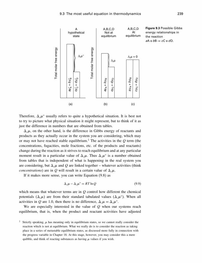
9.3 The most useful equation in thermodynamics 239
(a) (b) (c)
Tot
al m
olar
free
ene
rgy
Tot
al m
olar
free
ene
rgy
Ahypothetical
state
A,B,C,DNot at
equilibrium
A,B,C,D At
equilibrium
∆rµ = 0∆rµ
∆rµ°
aµ° A
+b
µ° B
cµ C
+ d
µ D
aµ A
+ b
µ B
cµC
+ d
µ D
aµA
+ b
µ B
cµ° C
+d
µ° D
Figure 9.3 Possible Gibbsenergy relationships inthe reactionaA+bB → cC+dD.
Therefore, �r�� usually refers to quite a hypothetical situation. It is best not
to try to picture what physical situation it might represent, but to think of it asjust the difference in numbers that are obtained from tables.�r�, on the other hand, is the difference in Gibbs energy of reactants and
products as they actually occur in the system you are considering, which mayor may not have reached stable equilibrium.2 The activities in the Q term (theconcentrations, fugacities, mole fractions, etc. of the products and reactants)change during the reaction as it strives to reach equilibrium and at any particularmoment result in a particular value of �r�. Thus �r�
� is a number obtainedfrom tables that is independent of what is happening in the real system youare considering, but �r� and Q are linked together – whatever activities (thinkconcentrations) are in Q will result in a certain value of �r�.
If it makes more sense, you can write Equation (9.8) as
�r�−�r�� = RT lnQ (9.9)
which means that whatever terms are in Q control how different the chemicalpotentials (�r�) are from their standard tabulated values (�r�
�). When allactivities in Q are 1.0, then there is no difference, �r�= �r��.
We are especially interested in the value of Q when our systems reachequilibrium, that is, when the product and reactant activities have adjusted
2 Strictly speaking, � has meaning only in equilibrium states, so we cannot really consider thereaction which is not at equilibrium. What we really do is to consider the reaction as takingplace in a series of metastable equilibrium states, as discussed more fully in connection withthe progress variable in Chapter 18. At this stage, however, you may consider this a merequibble, and think of reacting substances as having � values if you wish.
240 The equilibrium constant
themselves spontaneously such that �r� = 0. In this state, the∏i a�ii term is
called K, instead of Q, and (9.8) becomes
0= �r�� +RT lnK
or
�r�� = −RT lnK (9.10)
Standard states usually refer to pure substances (except for the aqueous standardstates) in which �=G, so this equation is often written
�rG� = −RT lnK (9.11)
This equation has been called, with some reason, the most useful in chem-ical thermodynamics, and it certainly merits the most careful attention. Mostimportant is the fact that the activity product ratio (K) on the right-hand sideis independent of variations in the system composition. Its value is controlledcompletely by a difference in standard (tabulated) state Gibbs energies (�rG
�)and so is a function only of the temperature and pressure. It is a constant for agiven system at a given temperature or temperature and pressure and is calledthe equilibrium constant. Its numerical value for a given system is not depen-dent on the system actually achieving equilibrium, or in fact even existing.Its value is fixed when the reacting substances are chosen. The left-hand siderefers to a difference in Gibbs energies of a number of different physical andideal states, which do not represent any real system or reaction. The right-handside, on the other hand, refers to a single reaction that has reached equilibrium,or more exactly, to the activity product ratio that would be observed if thesystem had reached equilibrium.
The great usefulness of Equation (9.11) lies in the fact that knowledge of afew standard state Gibbs energies allows calculation of an indefinite numberof equilibrium constants. Furthermore, these equilibrium constants are veryuseful pieces of information about any reaction. If K is very large, it tends toshows that a reaction will tend to go “to completion,” that is, mostly productswill be present at equilibrium, and if K is small, it tends to show that thereaction hardly goes at all before enough products are formed to stop it.3 If youare a chemical engineer designing a process to produce some new chemical,it is obviously of great importance to know to what extent reactions shouldtheoretically proceed. The equilibrium constant, of course, will never tell youwhether reactants will actually react, or at what rate; there may be some reasonfor reaction kinetics being very slow. It indicates the activity product ratio atequilibrium, not whether equilibrium is easily achievable.
3 These are just generalizations which are not always true, because the activities of products andreactants at equilibrium can be very large or very small. We emphasize this a bit more in theboxed statement on page 266.
9.3 The most useful equation in thermodynamics 241
Finally, NEVER write Equation (9.11) as
�rG=−RT lnK
that is, omitting the superscript �, because doing so indicates a complete lackof understanding of the difference between �rG and �rG
� and is just aboutgrounds for failing any course in this subject.
Let’s go over it once more. �rG� (or �r��) is the difference in Gibbs energy
between products and reactants when they are all in their reference states (puresolids and liquids, solutes at ideal 1 molal, gases at 1 bar), determined directlyfrom the tables. Products and reactants are virtually never at equilibrium witheach other under these conditions (�rG
� or �r�� never becomes equal to
zero). �rG (or �r�) is the difference in free energy between products andreactants in the general case (when at least one of the products or reactants isnot in its reference state) and becomes equal to zero when the reaction reachesequilibrium. �rG cannot be used in place of �rG
� in (9.11) because this wouldmean, among other things, that every reaction at equilibrium (�rG= 0) wouldhave an equilibrium constant of 1.0.
9.3.1 A first example
Let’s calculate the equilibrium constant for reaction (9.2),
H2CO3�aq�= HCO−3 �aq�+H+�aq�
First we write, as before,
�rG� = �fG
�HCO−
3+�fG
�H+ −�fG
�H2CO3
Getting numbers from the tables, we find
�rG� = −586�77+0− �−623�109�
= 36�339kJmol−1
= 36399 Jmol−1
The fact that this number is positive is not as significant as in our previousexamples. In this case it means that if H2CO3, HCO
−3 , and CO2−
3 were allpresent in an ideal solution, and each had a concentration of 1 molal, thereaction would go to the left. This hypothetical situation is not of much interest.We want the value of K.
Inserting this result in Equation (9.11), we get
�rG� = −RT lnK
36339=−�8�3145×298�15� lnK
242 The equilibrium constant
so
lnK =−36339/�8�3145×298�15�
=−14�659
or K = 4�30 ·10−7
= 10−6�37
If you don’t like dealing with natural logarithms, you can use the conversionfactor logx = ln x/2�30259 (Appendix A). This gives
logK =−36339/�2�30259×8�3145×298�15�
=−6�37
directly.This means that when these three aqueous species are at equilibrium,
aHCO−3·aH+
aH2CO3
= 10−6�37
This is the answer to our question in §9.1 (“what happens to the reaction afterit starts?”). The reaction continues until the ratios of the activities of the productsand reactants equals the equilibrium constant, in this case 10−6�37. It doesn’tmatter what the starting activities were, and individual activities at equilibriumcan be quite variable. In other words the values of aH2CO3
and of �aHCO−3·aH+�
are not determined, nor are the values of aHCO−3or aH+ individually; only the
ratio expressed by K is fixed. In specific cases, the values of these individualactivities are determined by the bulk composition of the solution, and can bedetermined by speciation (Chapter 16). For now, we are content to determineK. In this case K is the ionization constant for carbonic acid, H2CO3. It is avery small number, meaning that carbonic acid is a weak acid.
9.4 Special meanings for K
Equilibrium constants are also sometimes equal to system properties of interest,such as vapor pressures, solubilities, phase compositions, and so on. This isbecause quite often it can be arranged that all activity terms drop out (are equalto 1.0) except the one of interest, which can then be converted to a pressure orcomposition.
9.4.1 K equal to a solubility
Quartz–water exampleIn our quartz–water example (Equation 9.3), the equilibrium constant expres-sion is
K = aH4SiO4
aSiO2a2H2O
(9.12)
9.4 Special meanings for K 243
At this point the expression is perfectly general, valid for any conditions,and K is calculable from Equation (9.11) if we know the Gibbs energies ofthe three species in their reference states. In this case we are dealing with purequartz and water saturated with quartz. The quartz is in its reference state, andthe water contains so little silica that it is almost pure.4 By our definitions then(Equations 8.30) aSiO2
= 1 and aH2O= 1. Therefore
K = aH4SiO4
= �mH4SiO4H4SiO4
�
=mH4SiO4assuming H4SiO4
= 1�0
This shows that assuming H4SiO4is 1.0, which happens to be an excellent
approximation in this case, we can calculate the concentration of silica (mH4SiO4)
in equilibrium with quartz, that is, the solubility of quartz.Following our routine, we write for the reaction as written
�rG� = �fG
�H4SiO4
−�fG�SiO2
−2�fG�H2O
(9.13)
Then, getting numbers from the tables,
�rG� = −1307�7− �−856�64�−2�−237�129�
= 23�198kJmol−1
= 23198 Jmol−1
Then
�rG� = −RT lnK
23198=−�8�3145×298�15� lnK
so
logK =−23198/�2�30259×8�3145×298�15�
=−4�064
Thus the molality of SiO2 in a solution in equilibrium with quartz is about10−4�064, or about 5.2 ppm.5
4 Dissolving minerals in water changes aH2Overy little. So while strictly speaking aH2O
is not1.0 when saturated with some mineral, this assumption is usually quite good.
5 If the molality of H4SiO4�aq� is x, then the molality of SiO2�aq� is also x, as there is 1 moleof SiO2 in each.
244 The equilibrium constant
Doing it backwardsSo we see that Gibbs energies can sometimes be used to calculate a solubility.The same calculation also works in the other direction, that is, measuring asolubility can be used to calculate a value of �rG
�. In the quartz–water case,the reaction is particularly simple, in that because the quartz and water areessentially pure phases, not only are aH2O
and aSiO2equal to 1.0, but their values
of �fG� are known, as shown above. Therefore, a value of �rG
� calculatedfrom a solubility measurement can be used to calculate �fG
� for aqueous silica.Thus if you measured the solubility of quartz to be 5.2 ppm at 25 �C, you coulduse (9.13) in the form
�fG�H4SiO4
= �fG�SiO2
+2�fG�H2O
+�rG� (9.14)
to calculate �fG�H4SiO4
= −1307�7kJmol−1, and as a matter of fact that isusually how this quantity is determined.
A strange procedureNote the strangeness of what we are doing here. On the left-hand side of�rG
� = −RT lnK (Equation 9.11) we enter the standard Gibbs energies ofthe reactants and products, which in this case includes �fG
� of H4SiO4 at aconcentration of one molal (its concentration in its standard state) in a hypo-thetical ideal solution, and on the right-hand side calculated its equilibriumconcentration, only a few ppm. Remember what we said in deriving the equi-librium constant–the left-hand side consists of tabulated reference state data;it has nothing to do with real systems or with equilibrium. But from thesedata, equilibrium activity ratios and sometimes compositions can be calculated.Think about it.
9.4.2 K equal to fugacity of a volatile species
Hematite–magnetite exampleThe next example is the same in principle. Consider the reaction6
6Fe2O3�s�= 4Fe3O4�s�+O2�g� (9.15)
for which the equilibrium constant is
K = a4Fe3O4aO2
a6Fe2O3
6 It is important in this reaction to note that we write oxygen as O2�g�, that is, oxygen gas.There are also data for dissolved oxygen, written O2�aq� which are of course completelydifferent. The same ambiguity does not exist for hematite and magnetite, but it is always agood idea to append the �g�, �aq�, �s�, or �l� symbols for clarity.
9.4 Special meanings for K 245
If the reaction involves pure hematite Fe2O3 and pure magnetite Fe3O4, thenxFe2O3
= 1 and xFe3O4= 1, so aFe2O3
= 1 and aFe3O4= 1. Therefore
K = aO2
= fO2
= PO2f
Assuming that the activity coefficient f is 1.0, again in this case an excellentapproximation, we can calculate the partial pressure of oxygen in a gas phasein equilibrium with the two minerals hematite and magnetite.
Following the routine, we write
�rG� = 4�fG
�Fe3O4
+�fG�O2
−6�fG�Fe2O3
= 4�−1015�4�+0−6�−742�2�
= 391�6kJmol−1
= 391600 Jmol−1
�rG� = −RT lnK
391600=−�8�3145×298�15� lnK
logK =−391600/�2�30259×8�3145×298�15�
=−68�40
So the oxygen fugacity in equilibrium with hematite and magnetite at 25 �C and1 bar is 10−68�40 bar. This is an incredibly small quantity, which would haveabsolutely no significance if it were simply a partial pressure, unconnectedto thermodynamics. A partial pressure of this magnitude would be producedby one molecule of oxygen in a volume larger than that of a sphere with adiameter of the solar system (§12.12). However, it is in fact a parameter inthe thermodynamic model, just as valid as any other part of the model. It canbe used, for example, to calculate other parameters that might be more easilymeasurable. For example, the reaction
CH4�g�+O2�g�= CO2�g�+2H2�g� (9.16)
is one that you might be interested in if you were studying the bottom muds inFigure 2.1c. The equilibrium constant for this is
�rG� = −394�359+2�0�− �−50�72�−0
=−343�639kJmol−1
=−343639 Jmol−1
logK = 343639/�2�30259×8�3145×298�15�
= 60�203
246 The equilibrium constant
which means that at equilibrium,
fCO2·f 2H2
fCH4·fO2
= 1060�203
Now 1060�203 is just as ridiculous as 10−68�40 in a sense. But if we insert thevalue fO2
= 10−68�40 into this expression, we get
fCO2
fCH4
f 2H2= 1060�203 ·10−68�40
= 10−8�20
which begins to look a little more reasonable. This tells you something abouthow the CO2/CH4 ratio varies with fH2
. For example, you could say that accord-ing to the thermodynamic model, if fO2
is controlled by hematite–magnetite,the CO2 and CH4 fugacities (partial pressures) are equal when fH2
is 10−4�1
bar, and this might in fact be a measurable quantity in the muds.The point is that by writing a few reactions and using thermodynamics,
your thoughts about what might be happening in the bottom muds or anyother environment take shape in a controlled fashion – controlled, that is, bythe implied hypothesis of chemical equilibrium. Your system may not be atcomplete equilibrium, but your model is, because that is a good place to start.And the fact that one of your thermodynamic parameters, such as fO2
, turnsout to be impossibly small or large does not make it ridiculous; it just meansyou won’t be able to measure it directly, and you might want to concentrateon other parameters to which your impossible one is connected by the model.
Muscovite exampleThe hematite–magnetite example is just one of a great variety of geologicallyimportant reactions in which the fugacity of one species is numerically equalto an equilibrium constant. That one species can be O2 as in the example, butit can also be another species, typically H2O, CO2, or H2. For example, theassemblage muscovite plus quartz reacts at high temperatures to andalusite plusK-feldspar in the reaction
KAl3Si3O10�OH�2�s�+SiO2�s�= Al2SiO5�s�+KAlSi3O8�s�+H2O�g� (9.17)
for which the equilibrium constant is
K = aAl2SiO5·aKAlSi3O8
·aH2O
aKAl3Si3O10�OH�2·aSiO2
= aH2O(minerals are pure so a= 1)
= fH2O
f �H2O
= fH2O(ideal gas std. state at P = 1 so f � = 1 bar)
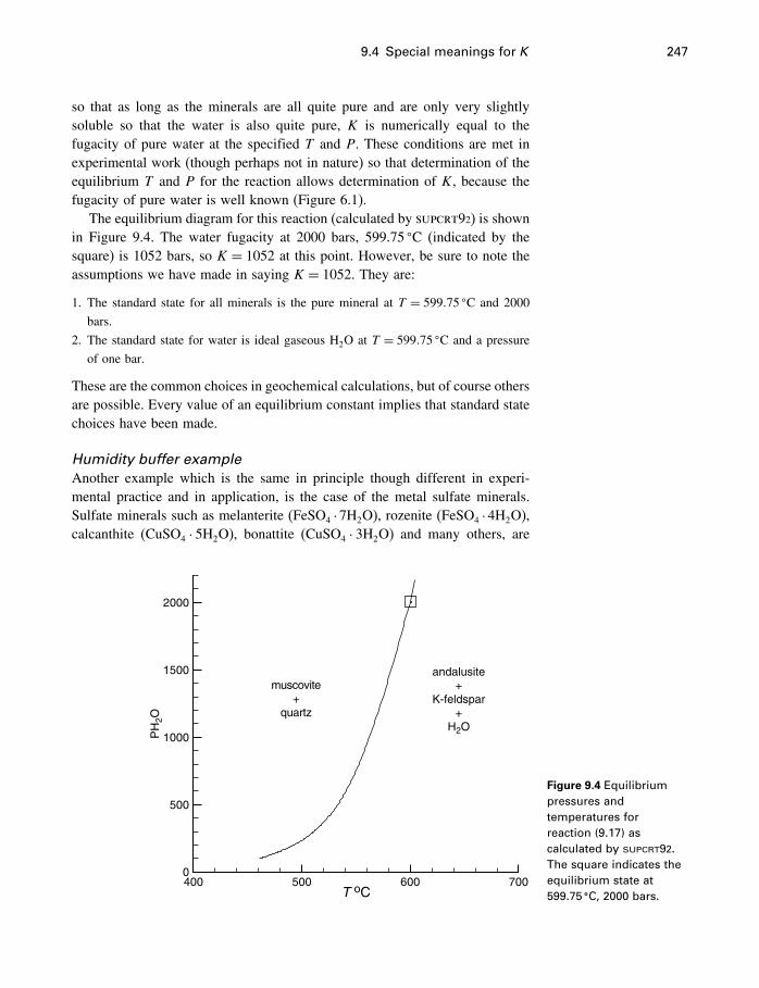
9.4 Special meanings for K 247
so that as long as the minerals are all quite pure and are only very slightlysoluble so that the water is also quite pure, K is numerically equal to thefugacity of pure water at the specified T and P. These conditions are met inexperimental work (though perhaps not in nature) so that determination of theequilibrium T and P for the reaction allows determination of K, because thefugacity of pure water is well known (Figure 6.1).
The equilibrium diagram for this reaction (calculated by supcrt92) is shownin Figure 9.4. The water fugacity at 2000 bars, 599.75 �C (indicated by thesquare) is 1052 bars, so K = 1052 at this point. However, be sure to note theassumptions we have made in saying K = 1052. They are:
1. The standard state for all minerals is the pure mineral at T = 599�75 �C and 2000
bars.
2. The standard state for water is ideal gaseous H2O at T = 599�75 �C and a pressure
of one bar.
These are the common choices in geochemical calculations, but of course othersare possible. Every value of an equilibrium constant implies that standard statechoices have been made.
Humidity buffer exampleAnother example which is the same in principle though different in experi-mental practice and in application, is the case of the metal sulfate minerals.Sulfate minerals such as melanterite (FeSO4 ·7H2O), rozenite (FeSO4 ·4H2O),calcanthite (CuSO4 · 5H2O), bonattite (CuSO4 · 3H2O) and many others, are
T oC
PH
2O
400 500 600 7000
500
1000
1500
2000
muscovite+
quartz
andalusite+
K-feldspar+
H2O
Figure 9.4 Equilibriumpressures andtemperatures forreaction (9.17) ascalculated by supcrt92.The square indicates theequilibrium state at599.75 �C, 2000 bars.
248 The equilibrium constant
Relative humidity and water activity
The relative humidity (RH) is defined as
RH= water vapor pressure� or PH2O
vapor pressure of pure liquid water� or P�H2O
This is usually reported as a percentage by multiplying by 100, i.e., %RH =RH× 100. Because the water vapor pressure and the water fugacity are almost
identical (Table 9.1), we can write
aH2O= fH2O
f �H2O
(std. state pure liquid water)
= PH2O
P�H2O
= RH
where f �H2Ois the fugacity of pure water. So measurements of RH are one form of
water activity. Alternatively, we can use ideal gaseous H2O at P = 1 bar standard
state, giving
aH2O= fH2O
1(std. state ideal gas H2O at 1 bar)
= RH×f �H2O
Both standard states are used in this type of work (Jerz and Rimstidt, 2003). They
give totally different values of lnK for reactions (Table 9.1).
common in mines, on mine tailings, and on sulfide minerals exposed to air.When these phases dissolve they create very acid solutions. They store metalsand sulfate during dry periods and dissolve readily during flushing events, caus-ing sudden increases in the acidity of drainage from abandoned mine sites withattendant environmental damage (Nordstrom and Alpers, 1999). It is thereforeimportant to have thermodynamic data for them in order to understand acidmine drainage situations.
The pressure of interest for reactions between these minerals is naturallyatmospheric pressure (1 bar) and the temperature of interest ranges from ambi-ent to the somewhat elevated temperatures that would occur in mine wastedumps (oxidation of sulfides is exothermic). Many of these hydrated sulfatesare stable only at water fugacities less than that of liquid water (they are not
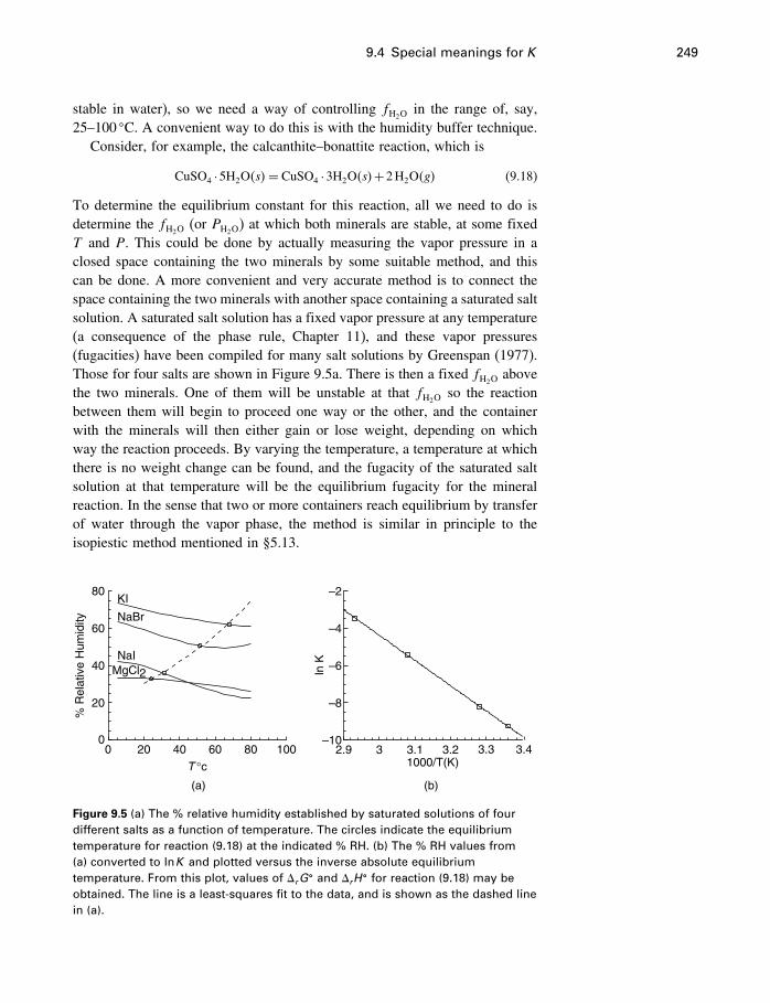
9.4 Special meanings for K 249
stable in water), so we need a way of controlling fH2Oin the range of, say,
25–100 �C. A convenient way to do this is with the humidity buffer technique.Consider, for example, the calcanthite–bonattite reaction, which is
CuSO4 ·5H2O�s�= CuSO4 ·3H2O�s�+2H2O�g� (9.18)
To determine the equilibrium constant for this reaction, all we need to do isdetermine the fH2O
(or PH2O) at which both minerals are stable, at some fixed
T and P. This could be done by actually measuring the vapor pressure in aclosed space containing the two minerals by some suitable method, and thiscan be done. A more convenient and very accurate method is to connect thespace containing the two minerals with another space containing a saturated saltsolution. A saturated salt solution has a fixed vapor pressure at any temperature(a consequence of the phase rule, Chapter 11), and these vapor pressures(fugacities) have been compiled for many salt solutions by Greenspan (1977).Those for four salts are shown in Figure 9.5a. There is then a fixed fH2O
abovethe two minerals. One of them will be unstable at that fH2O
so the reactionbetween them will begin to proceed one way or the other, and the containerwith the minerals will then either gain or lose weight, depending on whichway the reaction proceeds. By varying the temperature, a temperature at whichthere is no weight change can be found, and the fugacity of the saturated saltsolution at that temperature will be the equilibrium fugacity for the mineralreaction. In the sense that two or more containers reach equilibrium by transferof water through the vapor phase, the method is similar in principle to theisopiestic method mentioned in §5.13.
1000/T(K)
ln K
2.9 3 3.1 3.2 3.3 3.4–10
–8
–6
–4
–2
% R
elat
ive
Hum
idity
0 20 40 60 80 1000
20
40
60
80
MgCl2
NaI
NaBr
KI
(a) (b)
T °c
Figure 9.5 (a) The % relative humidity established by saturated solutions of fourdifferent salts as a function of temperature. The circles indicate the equilibriumtemperature for reaction (9.18) at the indicated % RH. (b) The % RH values from(a) converted to lnK and plotted versus the inverse absolute equilibriumtemperature. From this plot, values of �rG
� and �rH� for reaction (9.18) may be
obtained. The line is a least-squares fit to the data, and is shown as the dashed linein (a).
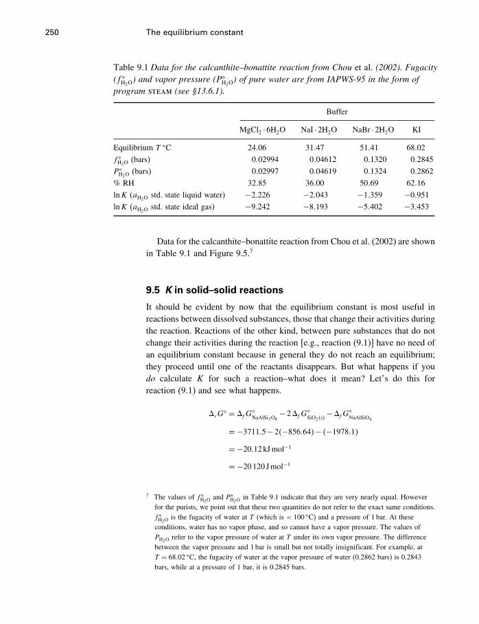
250 The equilibrium constant
Table 9.1 Data for the calcanthite–bonattite reaction from Chou et al. (2002). Fugacity(f �
H2O) and vapor pressure (P�
H2O) of pure water are from IAPWS-95 in the form of
program steam (see §13.6.1).
Buffer
MgCl2 ·6H2O NaI ·2H2O NaBr ·2H2O KI
Equilibrium T �C 24�06 31�47 51�41 68�02
f �H2O(bars) 0�02994 0�04612 0�1320 0�2845
P�H2O
(bars) 0�02997 0�04619 0�1324 0�2862
% RH 32�85 36�00 50�69 62�16
lnK (aH2Ostd. state liquid water) −2�226 −2�043 −1�359 −0�951
lnK (aH2Ostd. state ideal gas) −9�242 −8�193 −5�402 −3�453
Data for the calcanthite–bonattite reaction from Chou et al. (2002) are shownin Table 9.1 and Figure 9.5.7
9.5 K in solid–solid reactions
It should be evident by now that the equilibrium constant is most useful inreactions between dissolved substances, those that change their activities duringthe reaction. Reactions of the other kind, between pure substances that do notchange their activities during the reaction [e.g., reaction (9.1)] have no need ofan equilibrium constant because in general they do not reach an equilibrium;they proceed until one of the reactants disappears. But what happens if youdo calculate K for such a reaction–what does it mean? Let’s do this forreaction (9.1) and see what happens.
�rG� = �fG
�NaAlSi3O8
−2�fG�SiO2�s�
−�fG�NaAlSiO4
=−3711�5−2�−856�64�− �−1978�1�
=−20�12kJmol−1
=−20120 Jmol−1
7 The values of f �H2Oand P�
H2Oin Table 9.1 indicate that they are very nearly equal. However
for the purists, we point out that these two quantities do not refer to the exact same conditions.f �H2O
is the fugacity of water at T (which is < 100 �C) and a pressure of 1 bar. At theseconditions, water has no vapor phase, and so cannot have a vapor pressure. The values ofPH2O
refer to the vapor pressure of water at T under its own vapor pressure. The differencebetween the vapor pressure and 1 bar is small but not totally insignificant. For example, atT = 68�02 �C, the fugacity of water at the vapor pressure of water (0.2862 bars) is 0.2843bars, while at a pressure of 1 bar, it is 0.2845 bars.
9.5 K in solid–solid reactions 251
logK = 20120/�2�30259×8�3145×298�15�
= 3�52
K = 3349
As usual, this means that at equilibrium,
aNaAlSi3O8
aNaAlSiO4a2SiO2
= 103�52
If we in fact have pure nepheline, pure albite and pure quartz involved inthe reaction, then we come up with the same answer as before. The activitiesof NaAlSi3O8, NaAlSiO4, and SiO2 are 1.0 by our definitions, so the ratioaNaAlSi3O8
/�aNaAlSiO4a2SiO2
� is fixed at 1.0 and can never be equal to 3349 – thethree pure minerals can never reach equilibrium at 25 �C, 1 bar. But suppose theminerals are not pure – suppose they are solid solutions. Albite (NaAlSi3O8)forms a solid solution with anorthite (CaAl2Si2O8) in the mineral plagioclase,and nepheline also usually occurs in a solid solution with kalsilite (KAlSiO4),so the mole fractions and hence the activities of both NaAlSi3O8 and NaAlSiO4
will generally be less than 1.0, even though there are pure minerals with thesecompositions. The activity is less than 1.0 when the minerals are not pure, butoccur as a components of solid solutions.
In this particular case, having aNaAlSi3O8less than 1.0 would not help to
achieve equilibrium. Equilibrium could only be achieved by lowering aNaAlSiO4
or aSiO2. For example, in the presence of pure nepheline and pure albite, aSiO2�s�
would have to be 0.0173 to achieve equilibrium. This of course could nothappen if quartz was present, but aSiO2
might be controlled in some other way,such as by the amount of dissolved SiO2 in a solution that is undersaturatedwith quartz. To calculate this SiO2 concentration, the reaction would be writtenusing SiO2�aq� rather than SiO2�s� (see page 253).
There is an important lesson here. When we write a chemical reaction, welook up a value of �fG
� for each chemical formulas. The values of �fG� are
determined for those chemical species in very particular states – pure solids,ideal 1 molal solution, and so on. If our reaction is concerned with those speciesin those particular states, then the result is directly applicable to our problem –the value of �rG is the same as the value of �rG
�, and the reaction accordinglywill go or not go. This case basically arises only when dealing with pure solids.When dealing with solutions (solid, liquid, or gaseous), �rG
� is only a startingpoint. The reacting species are never in their reference states and have valuesof Gibbs energy that add up to �rG, not �rG
�. The chemical formulas in ourreactions represent species in some kind of solution, and we deal with thesesolutions with our activity terms, which are basically concentrations.
Reactions between solid phases such as (9.1) are in principle no differentfrom any other kind of reactions, such as (9.2). The only difference is that there
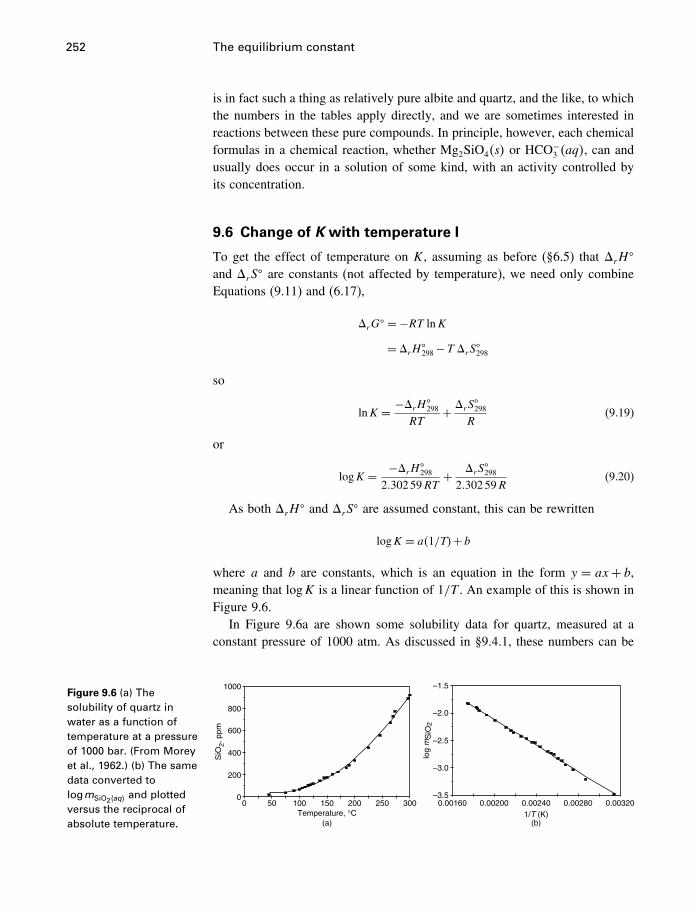
252 The equilibrium constant
is in fact such a thing as relatively pure albite and quartz, and the like, to whichthe numbers in the tables apply directly, and we are sometimes interested inreactions between these pure compounds. In principle, however, each chemicalformulas in a chemical reaction, whether Mg2SiO4�s� or HCO
−3 �aq�, can and
usually does occur in a solution of some kind, with an activity controlled byits concentration.
9.6 Change of K with temperature I
To get the effect of temperature on K, assuming as before (§6.5) that �rH�
and �rS� are constants (not affected by temperature), we need only combine
Equations (9.11) and (6.17),
�rG� = −RT lnK
= �rH�298−T �rS�298
so
lnK = −�rH�298
RT+ �rS
�298
R(9.19)
or
logK = −�rH�298
2�30259RT+ �rS
�298
2�30259R(9.20)
As both �rH� and �rS� are assumed constant, this can be rewritten
logK = a�1/T�+b
where a and b are constants, which is an equation in the form y = ax+ b,meaning that logK is a linear function of 1/T . An example of this is shown inFigure 9.6.
In Figure 9.6a are shown some solubility data for quartz, measured at aconstant pressure of 1000 atm. As discussed in §9.4.1, these numbers can be
Figure 9.6 (a) Thesolubility of quartz inwater as a function oftemperature at a pressureof 1000 bar. (From Moreyet al., 1962.) (b) The samedata converted tologmSiO2�aq� and plottedversus the reciprocal ofabsolute temperature.
00
200
400
600
800
1000
50 100 150 200 250 300
SiO
2, p
pm
Temperature, °C(a)
–3.5
–3.0
–2.5
–2.0
–1.5
0.00160 0.00200 0.00240 0.00280 0.003201/T (K)
log
mS
iO2
(b)
9.6 Change of K with temperature I 253
Calculation of aqueous silica
What is the silica content of a solution in equilibrium with plagioclase and
nepheline solid solutions at 25 �C and 1 bar? The activities of the solid solution
components are
aNaAlSiO4= 0�75
aNaAlSi3O8= 0�5
The reaction is Equation (9.1) as before, except that we must use SiO2�aq� rather
than SiO2�s�. Thus we write
NaAlSiO4�s�+2SiO2�aq�= NaAlSi3O8�s�
Getting data from Appendix B,
�rG� = �fG
�NaAlSi3O8
−2�fG�SiO2�aq�
−�fG�NaAlSiO4
=−3711�5−2�−833�411�− �−1978�1�
=−66�578kJmol−1
Then
logK =−�−66578�/�2�30259×8�3145×298�15�
= 11�664
K = 1011�664
= aNaAlSi3O8
aNaAlSiO4a2SiO2�aq�
= 0�5/�0�75×a2SiO2�aq��
aSiO2�aq�= �0�5/�1011�664×0�75��1/2
= 10−5�92
So assuming SiO2�aq� = 1, mSiO2�aq� in equilibrium with these two solid solutions
is 10−5�92 molal, slightly less than would be in equilibrium with the pure minerals.
• This is quite a hypothetical situation. Solid solutions with these activities are
common, but based on experience, they would never equilibrate with aqueous
silica at 25 �C. However at higher temperatures, such equilibria are common.• We used SiO2�aq� here, but H4SiO4 in Equation (9.12). We discuss this in
§9.10.
254 The equilibrium constant
interpreted as values of the equilibrium constant for the quartz dissolution reac-tion. The same data plotted as logmSiO2�aq�
versus 1/T , where T is in kelvins,are shown in Figure 9.6b. Obviously this shows a good linear correlation,indicating that �rH
� does not change greatly over the temperature range of25–300 �C.
9.6.1 Another example
As an example of the effect of T on K, as well as some of the other points wehave made, consider the reaction
CaCO3�s�+SiO2�s�= CaSiO3�s�+CO2�g� (9.21)
This is an important reaction at high temperatures, when granites intrude lime-stones at depth in the Earth, but we will consider it at low temperatures and1 bar pressure.
log K versus 1/T
A plot of logK versus 1/T can be used to obtain an estimate of �rH� for
the reaction for which K is the equilibrium constant. According to the authors
(Morey et al., 1962), the slope of the line in Figure 9.6b (fitted by the method of
least squares) is −1180K, and so from (8.14),
�rH�
2�30259R=−�−1180�
and
�rH� = 1180×2�30259×8�3145
= 22590 Jmol−1
≈ 22�6kJmol−1
However, although the data may appear to be quite linear, confirming a constant
�rH� and �rS�, you must realize that a gentle curvature can easily be obscured
by small random experimental errors, and even a gentle curvature implies a
significant change in slope and of �rH�. In this case, a theoretical treatment of
these and other data (contained in program supcrt92, Johnson et al., 1992) shows
that �rH� can vary (at 1 kbar) from 35.2 kJmol−1 at 25 �C to 23.2 kJmol−1 at
300 �C, while retaining an excellent fit to the data. It follows that exceptionally
accurate values of K are needed to give accurate values of �H� and �S� by
this method (Prue, 1969). The assumption of constant �rH� is not suitable for
accurate work, but is often useful nonetheless.
9.6 Change of K with temperature I 255
First, we get the equilibrium constant, as usual,
�rG� = �fG
�CaSiO3
+�fG�CO2
−�fG�CaCO3
−�fG�SiO2
=−1549�66+ �−394�359�− �−1128�79�− �−856�64�
= 41�411kJmol−1
= 41411 Jmol−1
�rG� = −RT lnK
41411=−�8�3145×298�15� lnK
logK298 =−41411/�2�30259×8�3145×298�15�
=−7�25
This means, as usual, thataCaSiO3
aCO2
aCaCO3aSiO2
= 10−7�25
and because all the solid phases are pure, their activities are all 1.0, and wewrite
aCO2= 10−7�25
= fCO2
Of course, both CaSiO3 (wollastonite) and CaCO3 (calcite) often form solidsolutions and in natural situations might have activities less than 1.0, as dis-cussed above. However, we are interested here in the pure phases.
The calculated fCO2of 10−7�25 can be thought of as meaning that if calcite,
wollastonite, and quartz were at equilibrium with a gas phase having a pressureof 1 bar at 25 �C, the partial pressure of CO2 in that gas would be about 10−7�25
or 5�6×10⁻⁸ bar. As long as the three minerals remain pure and at equilibrium,the equilibrium constant will continue to be equal to fCO2
, and so we cancalculate the temperature at which the CO2 pressure (fugacity) will reach 1 barby calculating the change in K with T .
To do this, we will first get another expression for the effect of T on K thatwill be more convenient. From (8.13) you can see that the slope of the graphof lnK as a function of 1/T is −�rH�/R, which is to say that at a temperatureof 298 K,
d lnKd�1/T�
=−�rH�298
R
Integrating this between 298 K and T , we get∫ T
298d lnK =−�rH
�298
R
∫ T
298d�1/T�
256 The equilibrium constant
and so
lnKT − lnK298 =−�rH�298
R
(1T− 1
298�15
)or
logKT = logK298−�rH
�298
2�30259R
(1T− 1
298�15
)(9.22)
By substituting terms, you can easily show that these are equivalent to our pre-vious equations, (9.19) and (9.20). Remember, they are valid only for constant�rH
� and �rS�.Now we need �rH
� for reaction (9.21). This is
�rH� = �fH
�CaSiO3
+�fH�CO2
−�fH�CaCO3
−�fH�SiO2
=−1634�94+ �−393�509�− �−1206�92�− �−910�94�
= 89�411kJmol−1
If we want to calculate the temperature T at which fCO2reaches 1 bar while
in equilibrium with calcite, quartz, and wollastonite, then KT = 1, logKT = 0,and using our value of �rH
�, we get
0=−7�25− 894112�30259×8�3145
(1T− 1
298�15
)from which T = 555 K or about 282 �C. The meaning of these calculations isillustrated in Figure 9.7.
Figure 9.7 The fugacity ofCO2 in equilibrium withcalcite, wollastonite, andquartz.
Calcite
Quartz
WollastoniteCalcite
Quartz
Wollastonite
Gas phase having
T = 25 °CP = 1 bar
T = 282 °CP = 1 bar
a CO2 partial pressure of 10–7.25 bar Pure CO2 gas phase
(a) (b)
9.7 Change of K with temperature II 257
A common error
You must remember that you CANNOT calculate lnK at T from
�rG�298 =−RT lnK [9.11]
where �rG� comes from the normal tables, simply by changing T from 298.15
to some other value. In this Equation (9.11) , �rG� and K must refer to the
same temperature. If you want K at some temperature other than 25 �C, firstget �rG
� at that new temperature from (6.17) or some other method, then getK from (9.11), using your new value of �rG
�T in place of �rG
�298. Of course,
this procedure has essentially been done for you in equations such as (9.20) and(9.22). An interesting exception to this rule is the case of some isocoulombicreactions (§9.7.2).
9.7 Change of K with temperature II
In Equation (9.11) we saw that lnK = −�rG�/RT , so that the effect of tem-
perature on K evidently depends on the effect of temperature on �rG�. In §9.6
we assumed a constant �H� and �S�, resulting in a simple linear relationshipbetween logK and 1/T . However, we also pointed out in §3.5.3 that
d�H
dT= �CP [3.23]
or
d�rH�
dT= �rC�
P (9.23)
and
d�rS�
dT= �rC
�P
T(9.24)
In other words, what we have really assumed is that�rC�P is zero, or that the heat
capacities of reactants and products are equal. However, if you look at measuredheat capacities, they look something like those shown in Figure 9.8. Puresolids, liquids, and gases generally have C�
P values that increase monotonically(constantly increasing) with T as illustrated by the mineral corundum. Over atemperature range of only 200 �C, the variation of C�
P may be fairly linear; over alarger range of T , it will show a distinct curvature. If the particular values of C�
P
of products and reactants in the reaction of interest happen to be about the sameand so cancel out, the �rC
�P = 0 approximation works well, but realistically
this only happens in fairly simple reactions such as calcite�aragonite, or bychance.
Furthermore, C�P for aqueous species behaves quite differently, always show-
ing a change in curvature as illustrated by HCl�aq� in Figure 9.8, so thatreactions having both minerals and aqueous species have virtually no chanceof having �rC
�P constant over a range of temperatures.
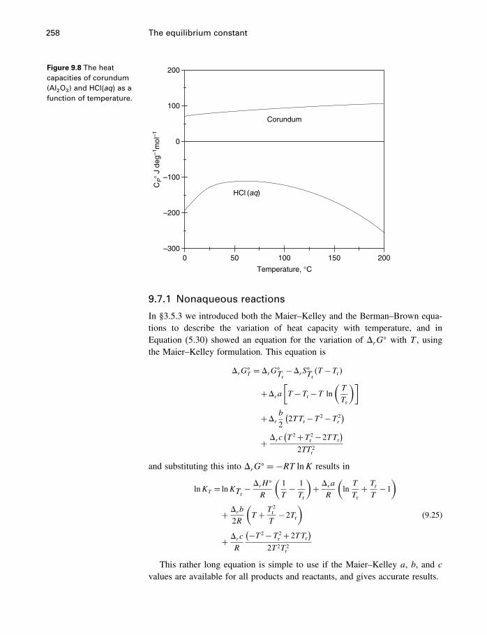
258 The equilibrium constant
Figure 9.8 The heatcapacities of corundum(Al2O3) and HCl�aq� as afunction of temperature.
–300
–200
–100
100
200
0
0 50 100 150 200
Temperature, °C
HCl (aq)
Corundum
CP
° J
deg–1
mol
–1
9.7.1 Nonaqueous reactions
In §3.5.3 we introduced both the Maier–Kelley and the Berman–Brown equa-tions to describe the variation of heat capacity with temperature, and inEquation (5.30) showed an equation for the variation of �rG
� with T , usingthe Maier–Kelley formulation. This equation is
�rG�T = �rG�
Tr−�rS�Tr �T −Tr�
+�ra[T −Tr −T ln
(T
Tr
)]+�r
b
2
(2TTr −T 2−T 2
r
)+ �rc
(T 2+T 2
r −2TTr)
2TT 2r
and substituting this into �rG� = −RT lnK results in
lnKT = lnKTr −�rH
�
R
(1T− 1Tr
)+ �ra
R
(lnT
Tr+ TrT
−1)
+ �rb2R
(T + T
2r
T−2Tr
)(9.25)
+ �rcR
(−T 2−T 2r +2TTr
)2T 2T 2
r
This rather long equation is simple to use if the Maier–Kelley a, b, and cvalues are available for all products and reactants, and gives accurate results.
9.7 Change of K with temperature II 259
9.7.2 Aqueous reactions
However, if your reactions contain aqueous species, the Maier–Kelley formu-lation does not apply, and a, b, and c values are not available because theydon’t work. The C�
P of HCl�aq� shown in Figure 9.8 is fairly typical of aqueousspecies, which are convex upward and have a maximum somewhere around50–100 �C (see also Figures 10.12; 15.10). If the aqueous and mineral speciesin your reaction are all in the supcrt92 database, you should use that program,which incorporates the HKF model, introduced in §13.6.2, and discussed morefully in Chapter 15. Failing that you must estimate your equilibrium constantas a function of T and P, and there are only a couple of ways of doing that.
Isocoulombic reactionsGenerally speaking, to model the change in logK with T you must account forthe change in C�
P for each species in the reaction individually, especially foraqueous species. However, it is sometimes possible to write the reaction suchthat equal numbers of ions appear on each side of the reaction or, failing that,the same total charge on each side, in which case a great deal of the variationwill cancel out. Such reactions are called “isocoulombic” (Mesmer and Baes,1974; Lindsay, 1980).
It is understood that the isocoulombic reaction has no solids or gases,because their variation of C�
P with T is quite different, as discussed above.The transformation from the reaction you are interested in to an isocoulombicreaction is made by combining your reaction with another one, which is oftenthe ionization of water reaction. For example,
H3PO4�aq�= H++H2PO−4
is a typical ionization reaction with all charges appearing on the right side. Theequilibrium constant for this reaction shows a considerable curvature, plottedas logK versus 1/T . Add to this the reaction
OH−+H+ = H2O�l�
and we have
H3PO4�aq�+OH− = H2PO−4 +H2O�l�
which has the same charge on both sides, and logK versus 1/T is rather closeto a straight line. Of course, to recover the desired ionization constant at somehigher temperature, you need to know the ionization constant for water as afunction of T in order to be able to “uncombine” it at the higher T . logK asa function of 1/T for isocoulombic reactions can be surprisingly accurate inmany cases.
Gu et al. (1994) have extended this method by noticing that the �C�P and
�S� terms for many isocoulombic reactions are not only small, but are often
260 The equilibrium constant
of opposite sign, and tend to cancel one another. Omitting the �S� term leadsto what they call the one-term extrapolation method. What this amounts to isthat for well-balanced aqueous reactions, �rG
� is independent of temperature,so that Equation (9.11) becomes
�rG�T = �rG
�Tr=−RT lnK (9.26)
so that only the Gibbs energy change of a reaction at 25 �C is sufficient tocalculate the value at any other temperature. A discussion of this method withexamples is given by Wood and Samson (1998).
The density modelFranck (1956, 1961) observed that the ionization constants of water and of manyaqueous solutes at elevated temperatures and pressures showed a remarkablylinear behavior when plotted as logK versus log� over wide ranges of T andP, where K is the equilibrium constant and � is the density of pure water.Since then this relationship and variations of it have been used in many studies(several references to these are in Anderson et al., 1991). Marshall and Franck(1981) used the expression
logK = a+b/T + c/T 2+d/T 3+ �e+f/T +g/T 2� log� (9.27)
to represent the ionization constant of water to 1000 �C with much success.Mesmer (1985, 1986) then showed that when this is simplified to include onlythe constants a, b and f , these parameters take on values fixed by the propertiesof water at some reference condition, and in Mesmer et al. (1987, 1988, 1989)that the resulting equation is quite successful in predicting solute properties toabout 300 �C. Anderson et al. (1991) give a more complete description, andinclude the data required to use the model equation.
Using only the a, b, and f terms, Equation (9.27) can be rewritten
lnK = p1+p2T
+ p3 ln�T
(9.28)
where p1, p2, and p3 are constants and � is the density of water at T and P.Because lnK is proportional to �rG
� (Equation 9.11) and ln� is specifiedat specific values of T and P, it follows that an expression relating lnK andln� is logically equivalent to one giving �rG
� as a function of T and P. InChapter 4 we saw that an equation giving �rG
� as a function of T and P iscalled a fundamental equation, and that it implicitly contains information onthe variation of all thermodynamic parameters with T and P. Therefore thereare implicit relationships between the parameters in both Equations (9.27) and(9.28) and all other thermodynamic parameters. These are given by Gates et al.(1982) for Equation (9.27).
Differentiation of Equation (9.28) with respect to temperature yields
�H� = −R�p2+p3�T+ ln��� (9.29)
9.7 Change of K with temperature II 261
where is the coefficient of thermal expansion of H2O (and V is the molarvolume),
= �1/V���V/�T�P = �� lnV/�T�P =−�� ln�/�T�Pand �H� is the standard enthalpy of reaction in a chosen reference state.Differentiating Equation (9.29) with respect to T at constant P gives
�C�P =−RTp3��/�T�P� or
p3 =−�C�
P
RT��/�T�P(9.30)
showing that Equation (9.28) implies that the quantity �C�P/RT��/�T�P is a
constant. This means that �C�P must mimic ��/�T�P . The value of p3 can be
determined by choosing values for T and P, that is, a reference state. Denotingthe reference state by subscript r, then
�C�P/RT��/�T�P = �C�
Pr/RTr��/�T�Pr
so that at any T and P, Equation (9.28) implies that
�C�P = �C�
Pr· T��/�T�PTr��/�T�Pr
(9.31)
Similarly, differentiation of Equation (9.28) with respect to pressure gives
�V � = −p3R�
= �C�Pr�
Tr��/�T�Pr
(9.32)
where � is the compressibility coefficient of water,
�= �1/V���V/�P�T = �� lnV/�P�T =−�� ln�/�P�T
Inserting this expression for the heat capacity into the standard expres-sions for enthalpy end entropy, Equations (3.31) and (5.21) gives expressionsfor �H�ãnd �S�, and combining these as �H� −T�S� gives �G� and fromthis logK. Comparing the expression for logK with Equation (9.28) givesexpressions for p1 and p2.
These and other relationships that follow from the model are summarized inthe box on page 263. This empirical formulas apparently works well because��/�T� as a function of temperature for water is U-shaped, which gives to theexpression for �rC
�P (if �C�
P is negative) an inverted-U shape with a maximumaround 100 �C, which is the same shape that the C�
P of many aqueous ions have(see Chapter 15). Furthermore the variation of �C�
P at higher pressures is alsofairly faithfully modeled by the expression for �C�
P, and the equations fit the
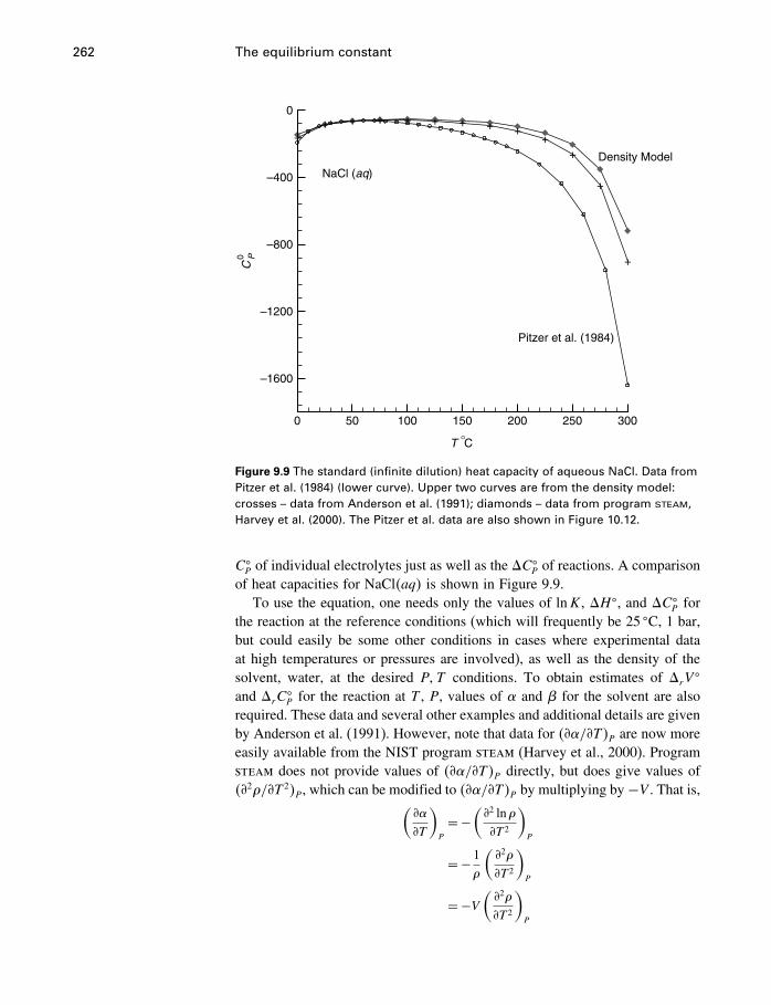
262 The equilibrium constant
++ + + + + + + +
++
+
+
T °C
CP0
0 50 100 150 200 250 300
–1600
–1200
–800
–400
0
NaCl (aq)
Pitzer et al. (1984)
Density Model
Figure 9.9 The standard (infinite dilution) heat capacity of aqueous NaCl. Data fromPitzer et al. (1984) (lower curve). Upper two curves are from the density model:crosses – data from Anderson et al. (1991); diamonds – data from program steam,Harvey et al. (2000). The Pitzer et al. data are also shown in Figure 10.12.
C�P of individual electrolytes just as well as the �C�
P of reactions. A comparisonof heat capacities for NaCl�aq� is shown in Figure 9.9.
To use the equation, one needs only the values of lnK, �H�, and �C�P for
the reaction at the reference conditions (which will frequently be 25 �C, 1 bar,but could easily be some other conditions in cases where experimental dataat high temperatures or pressures are involved), as well as the density of thesolvent, water, at the desired P�T conditions. To obtain estimates of �rV
�
and �rC�P for the reaction at T , P, values of and � for the solvent are also
required. These data and several other examples and additional details are givenby Anderson et al. (1991). However, note that data for ��/�T�P are now moreeasily available from the NIST program steam (Harvey et al., 2000). Programsteam does not provide values of ��/�T�P directly, but does give values of��2�/�T 2�P , which can be modified to ��/�T�P by multiplying by−V . That is,(
�
�T
)P
=−(�2 ln��T 2
)P
=− 1�
(�2�
�T 2
)P
=−V(�2�
�T 2
)P
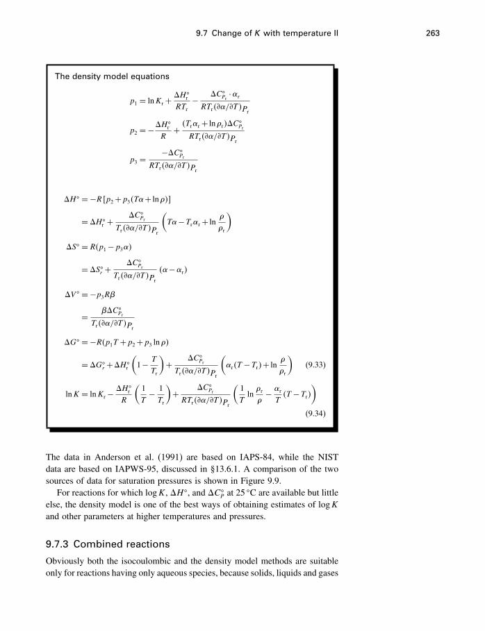
9.7 Change of K with temperature II 263
The density model equations
p1 = lnKr +�H�
r
RTr− �C�
Pr·r
RTr��/�T�Pr
p2 =−�H�r
R+ �Trr + ln�r��C
�Pr
RTr��/�T�Pr
p3 =−�C�
Pr
RTr��/�T�Pr
�H� = −R�p2+p3�T+ ln���
= �H�r +
�C�Pr
Tr��/�T�Pr
(T−Trr + ln
�
�r
)�S� = R�p1−p3�
= �S�r +�C�
Pr
Tr��/�T�Pr
�−r�
�V � = −p3R�
= ��C�Pr
Tr��/�T�Pr
�G� = −R�p1T +p2+p3 ln��
= �G�r +�H�
r
(1− T
Tr
)+ �C�
Pr
Tr��/�T�Pr
(r�T −Tr�+ ln
�
�r
)(9.33)
lnK = lnKr −�H�
r
R
(1T− 1Tr
)+ �C�
Pr
RTr��/�T�Pr
(1Tln�r�− r
T�T −Tr�
)(9.34)
The data in Anderson et al. (1991) are based on IAPS-84, while the NISTdata are based on IAPWS-95, discussed in §13.6.1. A comparison of the twosources of data for saturation pressures is shown in Figure 9.9.
For reactions for which logK, �H�, and �C�P at 25 �C are available but little
else, the density model is one of the best ways of obtaining estimates of logKand other parameters at higher temperatures and pressures.
9.7.3 Combined reactions
Obviously both the isocoulombic and the density model methods are suitableonly for reactions having only aqueous species, because solids, liquids and gases
264 The equilibrium constant
have heat capacities with a quite different temperature variation. For reactionshaving both pure phases and aqueous species, the heat capacity expressionscan be simply combined.
For reactions in which the aqueous species are “isocoulombic” but mineralsor other phases are also present, one simply uses the Maier–Kelley expressionfor logK, Equation (9.25), whether or not the pure phases in the reactionare compositionally balanced. For the density model, two expressions for thevariation of logK are combined, giving
lnKT = lnKTr −�rH
�
R
(1T− 1Tr
)+ �ra
R
(lnT
Tr+ TrT
−1)
+�rb
2R
(T + T
2r
T−2Tr
)
+�rc
R
(−T 2−T 2r +2TTr
)2T 2T 2
r
(9.35)
+ �C�Pr
RTr��/�T�Pr
(1Tln�r�− r
T�T −Tr�
)where a�b� c are Maier–Kelley heat capacity coefficients and �C�
Prrefers to
aqueous species only.However, Anderson (1995) notes that it is often advantageous to use the
model, not on the overall reaction, but on individual species. This makes iteasier to add parameters calculated by Maier–Kelley or some other method. Inusing the density model with individual species and minerals, it is advisable tocalculate high T , P Gibbs energies and later combine these to the desired logKvalues. This should be done with a slightly different version of Equation (9.33)[substitute −S�r �T −Tr� for �H�
r �1−T/Tr�] and Equation (5.33) for the purephases. This ensures that all species use the same convention for Gibbs energies.
9.8 Change of K with pressure
The variation of the equilibrium constant with pressure depends of courseon how standard states are defined, because this controls how �rG
� and theactivity terms in K vary with pressure. This was discussed in some detail inconnection with activities (§8.3). To briefly summarize, if the standard statesof all the reaction species are defined as fixed at 1 bar (or conceivably someother pressure), then K does not vary with P; it is a constant at a given T .If the standard states are defined as variable in P, then K does vary withP. This variation takes different forms, depending on whether the reactionspecies are solid, liquid, gaseous, or aqueous, and is best handled by calculatingthe variation of each individual species activity with P, then combining theminto K.
Surprisingly, it is not often necessary to do this, because applications com-monly provide data along isobars, so that only the temperature variation is of
9.9 The amino acid example again 265
interest. Each isobar has its own standard state pressure, so it is not necessaryto calculate the change in activities or equilibrium constants between isobars.
The only commonly used relation between pressure and the equilibriumconstant is the case where all reactants and products are solids. Assuming thesolids are incompressible, applying relation (5.32) to each of the terms in �rG
�
results in
� lnK�P
=− ��rG�
�P/RT
=−�rV �/RT
so that
lnKP2 = lnKP1 −�rV
�
RT�P2−P1� (9.36)
9.9 The amino acid example again
Let’s write Equation (5.14) one more time.
C8H16N2O3�aq�+H2O�l�= C6H13NO2�aq�+C2H5NO2�aq� (9.37)
or
leucylglycine+water = leucine+glycine (9.38)
�rG� = �fG
�leucine
+�fG�glycine
−�fG�leucylglycine
−�fG�water
=−13903 Jmol−1
We now know that our calculation of this �rG� (§5.5.2), the reaction in which
a peptide bond between two amino acids is broken, was only a beginning.The value of −13903 Jmol−1 means that if all reactants and products had unitactivity (leucine, glycine, and leucylglycine had concentrations of 1 molal,and water was pure), the reaction would start to go to the right; leucylglycinewould start to break down to leucine and glycine. But we note again thefundamental difference between this reaction between dissolved compounds,and reaction (9.1) between solid compounds. Repeating (9.1) here,
NaAlSiO4�s�+2SiO2�s�= NaAlSi3O8�s� (9.39)
�rG� = �fG
�NaAlSi3O8
−�fG�NaAlSiO4
−2�fG�SiO2
=−20�12kJmol−1
266 The equilibrium constant
The value of �rG� of −20120 Jmol−1 means that reaction (9.39) will also
go to the right. But this reaction will continue to go (strictly, it should continueto go, according to our model) until either NaAlSiO4�s� or SiO2�s� is used up.Thus NaAlSiO4�s� and SiO2�s� are not stable together – one of them mustdisappear.
This is not the case with leucylglycine. We cannot say that leucylglycine isnot stable in water–what happens to it depends entirely on its concentration andon the concentrations of other things in solution such as leucine and glycine.The unit activities are only a starting point, and a very unrealistic one at that.The next step is to calculate the equilibrium constant for (9.37)
�rG� = −RT lnK
−13903=−�8�3145×298�15� lnK
logK298 = 13903/�2�30259×8�3145×298�15�
= 2�436
Thus
aleucine aglycine
aleucylglycine awater= 102�436
The activity (mole fraction) of water in biochemical systems is usually closeto 1.0, so we see that although leucylglycine is not “unstable” in water, itsconcentration at equilibrium must be quite a bit less than that of its constituentamino acids. For example, if leucine and glycine had concentrations of say10−3m (activities of 10−3), the equilibrium activity of leucylglycine wouldbe 10−8�436 (concentration 10−8�436m). So with concentrations of 10−3, 10−3,and 10−8�436, leucine, glycine, and leucylglycine would not react at all, butwould be at equilibrium. In fact, with a concentration of leucylglycine of lessthan 10−8�436, the reaction as written would go to the left – leucylglycine wouldform from the two amino acids. So remember this – unless the reaction consistsonly of pure phases,
You cannot reliably tell which way the reaction will go by looking at �rG�.
You can always tell which way the reaction will go by looking at �rG.Look at Equation (9.8) one more time. When leucine, glycine, leucylglycine,
and water all have unit activities, (9.8) becomes
�r�= �r�� +RT lnQ
−13903=−13903+RT ln(1×11×1
)
9.9 The amino acid example again 267
In other words, �r� is the same as �r��; the driving force for the reaction
can be obtained directly from the tables, as for solid–solid reactions. Whenproducts and reactants have reached equilibrium,
�r�= �r�� +RT lnK
0=−13903+RT ln(10−3×10⁻³
10−8�436×1
)Now the lnK term exactly balances the �r�
� term, and the driving force for thereaction is zero. Ifaleucylglycine< 10−8�436, thedriving force (�r�) becomespositive.
9.9.1 Peptides favored at higher temperatures
To round out our discussion of this reaction, let’s calculate the effect of tem-perature on the equilibrium constant in reaction (8.18). From Appendix B wefind the following data:
Substance Formulas �fH�� Jmol−1 S�� Jmol−1 K−1
leucine C6H13NO2�aq� −632077 215.48glycine C2H5NO2�aq� −513988 158.32leucylglycine C8H16N2O3�aq� −847929 299.16water H2O�l� −285830 69.91
�rH� = �fH
�leucine
+�fH�glycine
−�fH�leucylglyine
−�fH�water
=−632077−513988− �−847929�− �−285830�
=−12306 Jmol−1
These aqueous species are not ionized, so perhaps our constant �rC�P assump-
tion will not be too bad over small temperature intervals. Suppose we wantedthe value of K at 100 �C. Equation (9.22) then becomes
logKT = logK298−�rH
�298
2�30259R
(1T− 1
298�15
)= 2�436− −12306
2�30259×8�3145
(1
373�15− 1
298�15
)= 2�00
Alternatively, by calculating �rS�, you could use Equation (6.17) first, then
Equation (9.11). Thus
�rS� = S�leucine+S�glycine−S�leucylglyine−S�water= 215�48+158�32−299�16−69�91
= 4�73 Jmol−1
268 The equilibrium constant
Then
�rG�373 = �rH
�298−T �rS�298
=−12306−373�15×4�73
=−14071 Jmol−1
from which
logK373 =−�rG
�373
2�30259RT
=− −140712�30259×8�3145×373�15
= 1�97
There will often be a small discrepancy in logK calculated in different ways,as here (2.00 versus 1.97), because of slight inconsistencies in the data. Inother words, to get answers that are exactly the same no matter which way thecalculation is done, the data in the tables for each compound must satisfy therelation
�fG� = �fH
� −298�15×�fS�
Because enthalpy, entropy, and Gibbs energy data come from different experi-ments, using a variety of methods, this relation is often not satisfied exactly inthe tabulated data.
The interesting aspect of this calculation of K is that according to the data,leucylglycine (and perhaps all peptide bonds in proteins) becomes more stableas temperature increases. Thus for the same concentrations of leucine andglycine (10−3m) as before, we find the leucylglycine concentration is 10−8�0m
at 100 �C, compared to 10−8�436m at 25 �C. That is, its concentration is morethan doubled. This result is quite interesting to those scientists trying to figureout how life could have begun in the early days of the Earth, 3.5 billion yearsago. The fact that increasing temperatures do not impair but in fact aid thebonding of simple amino acids, the building blocks of life, has led to thoughtsthat perhaps life began when the oceans were at higher temperatures, or inparticular locations (volcanic environments) where heat was available.
This result is typical of the value of thermodynamics. It does not and cannottell you how life began, but it can tell you which processes are possible andwhich impossible, and what the effects of changing the constraints on yoursystem will be. This guides the development of scientific ideas in an essentialway and provides a universally agreed-upon bedrock from which to start.However, it is up to you to think of the processes to ask thermodynamics about,and this is the creative part of science.
9.10 Some conventions regarding components 269
9.10 Some conventions regarding components
There are two ways in which the way chemical formulas are used which mayprove confusing:
1. Aqueous species are used in both hydrated and nonhydrated forms. For example,
dissolved silica is written as SiO2�aq� or as SiO2 · 2H2O (or H4SiO4, which is the
same thing).
2. Formulas can be presented in various multiples. For example forsterite may be listed
as Mg2SiO4 or as MgSi0�5O2.
These are quite simple relationships, but they can cause quite a bit of confusion.
9.10.1 Hydrated versus nonhydrated species
H4SiO4 exampleOne way to write the dissolution reaction for quartz is
SiO2�s�+2H2O= H4SiO4�aq� (9.40)
Another way to write the same reaction is
SiO2�s�= SiO2�aq� (9.41)
The only difference between these two ways of writing a reaction for thedissolution of quartz is that in (9.40) we have assumed that the dissolvedsilica is in the form of a molecule containing one SiO2 attached to two H2Omolecules, whereas in (9.41) we have made no assumption as to the form ofthe dissolved silica. So what do we actually know about dissolved silica? Whatwe know, besides the concentrations under various conditions, is that
1. Under most conditions, the aqueous silica molecule has only one Si (i.e., it is
monomeric, not polymeric), and
2. Except in very basic solutions it is uncharged, electrically neutral.
We might as well then write a formulas for this species that is as simple aspossible, while observing these two facts, and SiO2�aq� does this. Therefore,SiO2�aq� does not refer to a species of dissolved silica which is not attached toany H2O or other molecules; it refers to the silica that exists as a monomericuncharged species of whatever nature in solution. It might be attached to twoH2O, or six H2O, or be a mixture of several such species; it doesn’t matter.
The other common formulas, H4SiO4�aq�, originates historically in the beliefthat Si in water must be tetrahedrally coordinated by oxygens, as it is in crystals.That may well be true, but there may be other oxygens in the form of H2Osalso attracted to the Si. The exact nature of the complexes of Si and manyother elements of interest is a continuing research topic. The important point
270 The equilibrium constant
from the thermodynamic point of view is that what we call the dissolved silica,whether H4SiO4�aq� or SiO2�aq�, doesn’t matter, because as long as we derivethe properties of each in a consistent manner, each will give the right answerin calculations.
In what way are the properties of these species different? Because thesetwo formulas refer to the same physical substance, dissolved silica, their con-centrations and activities are identical. But because they are related by theequation
SiO2�aq�+2H2O�l�= H4SiO4�aq�
their standard state properties such as �fG� and �fH
� must be different byexactly twice the corresponding property of H2O�l�. Thus
�fG�H4SiO4�aq�
= �fG�SiO2�aq�
+2�fG�H2O�l�
The Gibbs energy of formation of H4SiO4 is defined as the sum of the Gibbsenergies of SiO2�aq� and (twice that of) H2O�l�. In other words, the rela-tionship between H4SiO4�aq� and SiO2�aq� is strictly a formal one. They arederived from the same experimental data and will yield the same results incalculations.
H2CO3 exampleThe same relationship also holds for other species. For example, when CO2
gas dissolves in water, it hydrolyzes (reacts with water) to a very small extent,forming some H2CO3 molecules in solution. It is rather difficult to determinethe exact amount of H2CO3, and this problem is avoided by simply callingthe total amount of carbon dioxide in solution either CO2�aq� or H2CO3�aq�,exactly as the dissolved silica is called SiO2�aq� or H4SiO4�aq�. Then for thesame reason as before, we find that
�fG�H2CO3�aq�
= �fG�CO2�aq�
+�fG�H2O�l�
Again, this relationship is strictly formal, although in this case it can be moreconfusing, because there is in fact some literature on the subject of how muchdissolved CO2 actually hydrolyzes to the species H2CO3 and how much remainsas CO2 molecules. In other words, H2CO3 is sometimes used as a species, andsometimes in the conventional sense we are discussing. The thermodynamicproperties of H2CO3 in these two senses will of course be completely different.In this book we use the conventional sense for H2CO3�aq�. Another way oflooking at this is to see H2CO3 as an alternative component, rather than as anaqueous species.
9.10 Some conventions regarding components 271
Al(OH)3 exampleAnother example is the aluminum species Al�OH�3�aq�. Again, this is amonomeric uncharged species of Al in solution. There is really no need toassume that it has three oxygens and three hydrogens attached to it. Whateveris attached to it, we can call it AlO1�5�aq�, whose properties will differ fromthose of Al�OH�3�aq� by those of 1�5H2O�l�, because
AlO1�5�aq�+1�5H2O�l�= Al�OH�3�aq�
and similarly for other aqueous aluminum species. Thus in basic solutions thedominant Al species can be referred to as Al�OH�−4 or as AlO−
2 . The essentialinformation is that the species is monomeric and has one negative charge.
9.10.2 What is a mole of olivine?
Another way that the choice of formulas can differ is that some choices canbe multiples of other choices. This is most often seen in choosing solutespecies in solids, because there are no “real” species, just a crystal structurethat is a solid solution. For example, the mineral olivine is a solid solution oftwo components, forsterite (Mg2SiO4) and fayalite (Fe2SiO4). The solution isrepresented by �Mg�Fe�2SiO4, because the Mg and Fe atoms share the samepositions in the crystal structure.
But what reason do we have to choose Mg2SiO4 and Fe2SiO4 as our compo-nents? The formulas simply shows us the stoichiometry of the components – theratios or relative amounts of the elements. Why not MgSi0�5O2, or Mg4Si2O8?The same question could also arise in discussing aqueous species, except inthat case we often have experimental evidence about the nature of the speciesin solution. That kind of evidence does not exist for the three-dimensionalcrystal structures of solid solutions – we are free to choose any component thatis stoichiometrically correct. Does it make any difference? Yes.
In §7.2 we noted that some confusion might arise in the definition of molefractions, but here the choice makes no difference. That is,
nFeSi0�5O2
nFeSi0�5O2+nMgSi0�5O2
= nFe2SiO4
nFe2SiO4+nMg2SiO4
So that is not the problem. The problem is that the choice of formulas, themole of substance, affects the energy content per mole and hence the activity.
Suppose our system consists of a certain mass (a crystal) of pure forsterite,Mg2SiO4. The Gibbs energy of the system is a finite, unknown quantity, whichdepends on the mass of the crystal. A crystal with twice the mass has a Gtwice as large. But the molar G does not vary with the size of the crystal. Themolar G is defined as G = G/n (§2.4.1), where n is the number of moles inthe crystal. The point is, the number of moles of what? Obviously the numberof moles of Mg2SiO4 in the crystal will be exactly half the number of moles of
272 The equilibrium constant
MgSi0�5O2 in the crystal, because Mg2SiO4 contains twice the number of atomsthat MgSi0�5O2 does. Therefore, GMg2SiO4
= 2GMgSi0�5O2. Or, if you prefer, you
can say that GMg2SiO4= 2GMgSi0�5O2
simply because it contains twice the massand, therefore, twice the energy of whatever kind.
This difference in the Gibbs energy of the mole is translated into a differencein activities. Because GMg2SiO4
= 2GMgSi0�5O2and G�
Mg2SiO4= 2G�
MgSi0�5O2, then
GMg2SiO4−G�
Mg2SiO4= 2 �GMgSi0�5O2
−G�MgSi0�5O2
�
and
RT lnaMg2SiO4= 2RT lnaMgSi0�5O2
and therefore
aMg2SiO4= a2MgSi0�5O2
The problem this poses can be seen in considering Raoult’s law, which wesaid was ai = xi. But if ai = a20�5i we have a problem. Because xi is independentof how we write the formulas for i, we see that ai and a0�5i cannot both be equalto xi, even if Raoult’s law is followed exactly. If a0�5i versus xi is a straightline, then ai versus xi will describe a parabola.
This is a well-known problem, and generally the formulas for components ischosen such that the simple statement of Raoult’s law is followed as closely aspossible. Again, this relationship between activities is entirely formal and tellsus nothing about forsterite or olivine. However, it is important to rememberthat choosing a formulas for your components has consequences for activities.
The problem is more difficult in other systems. How does one choosecomponents in a complex silicate melt, for example? In a melt there are nostoichiometric restrictions to be observed, but the formal relationship betweenthe activities of various component choices that we have discussed remainstrue. So if you measure the activity of some component in a melt, and determinethe deviations of these activities from Raoult’s law by calculating activitycoefficients, the question is, what part of these activity coefficients representsnonideal behavior, and what part represents a poor choice of components?Generally speaking, extremely large or extremely small activity coefficientsmean that the component involved has been badly chosen, which is to say thatit does not come very close to representing the “real” situation in the system.In these situations, thermodynamics provides no help whatsoever. It pointsout the consequences of choices relative to each other, and from there on theinvestigator is on her own. In other words, the choice of components, as muchas the choice of system to investigate, is a part of the “art of doing science,”that part which relies on skill and intuition, and can never be taught.
9.11 Summary 273
9.11 Summary
This chapter contains a sudden increase in the amount of practical, usablematerial. If you ever have occasion to use thermodynamics in a practicalsituation, it will very likely involve the use of the equilibrium constant.
The molar Gibbs energy of a dissolved substance changes with the con-centration of the substance. The activity is a dimensionless concentration-liketerm that is used to give the Gibbs energy in a particular state, in terms ofits difference from its value in some reference state (Equation 7.37). Whena reaction has reached equilibrium, the activities of the various products andreactants can have a variety of values individually, but their ratio, as expressedin the equilibrium constant K, has a fixed and calculable value.
The equilibrium constant is calculated from numbers (Gibbs energies) takenfrom tables of standard data (derived experimentally, as discussed in Chapter 5).These standard data give the term �r�
� or �rG�, which is a constant for a
given T and P. It has nothing to do with whether your system or reaction hasreached equilibrium (�r�= 0) or not. However, it can be used to calculate K,which gives the ratio of product and reactant activities your reaction will haveif it ever reaches equilibrium.
The superscript � therefore has considerable significance. It should not beomitted or inserted carelessly in your calculations.
10Real solutions
10.1 Introduction
We have now considered both ideal solution behavior and deviations from this,but in a rather generalized way, using activity coefficients. We now have tostart to consider how to measure these things, and doing this means we haveto consider partial molar properties in much more detail.
We start with a fairly detailed look at the volumetric properties of solutions,because these are the most intuitive. Partial molar properties of the other statevariables are the same in principle, but become more complicated in the caseof enthalpy measurements because of its relative nature. The Gibbs energy isalso a relative property, but is treated in quite a different way.
Most of the material in this chapter is quite general, and can be applied toany kind of solution, although most of our examples are for aqueous solutions.The properties of electrolyte solutions introduce complications, discussed inChapter 15. The properties of real gaseous solutions are often handled by“equations of state,” the subject of Chapter 13, and those of solid solutionshave some unique aspects, discussed in Chapter 14.
10.2 Solution volumes
All real solutions are of course nonideal. Our discussion of their propertieswill be concerned for the most part with deviations from the properties of idealsolutions, whether Henryan or Raoultian.
10.2.1 Partial and apparent properties
The properties of a dissolved substance are described in terms of partial,apparent, and excess total or molar properties, so we begin by discussing theseterms, using volume as an example.
The volume of mixingIf two substances are immiscible (they do not dissolve into one another to anyappreciable extent, like oil and water), obviously the volume of the two together
274
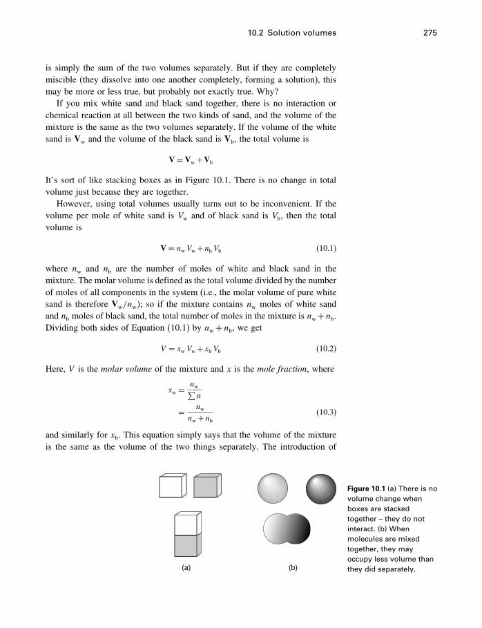
10.2 Solution volumes 275
is simply the sum of the two volumes separately. But if they are completelymiscible (they dissolve into one another completely, forming a solution), thismay be more or less true, but probably not exactly true. Why?
If you mix white sand and black sand together, there is no interaction orchemical reaction at all between the two kinds of sand, and the volume of themixture is the same as the two volumes separately. If the volume of the whitesand is Vw and the volume of the black sand is Vb, the total volume is
V= Vw+Vb
It’s sort of like stacking boxes as in Figure 10.1. There is no change in totalvolume just because they are together.
However, using total volumes usually turns out to be inconvenient. If thevolume per mole of white sand is Vw and of black sand is Vb, then the totalvolume is
V= nw Vw+nb Vb (10.1)
where nw and nb are the number of moles of white and black sand in themixture. The molar volume is defined as the total volume divided by the numberof moles of all components in the system (i.e., the molar volume of pure whitesand is therefore Vw/nw); so if the mixture contains nw moles of white sandand nb moles of black sand, the total number of moles in the mixture is nw+nb.Dividing both sides of Equation (10.1) by nw+nb, we get
V = xw Vw+xb Vb (10.2)
Here, V is the molar volume of the mixture and x is the mole fraction, where
xw = nw∑n
= nwnw+nb
(10.3)
and similarly for xb. This equation simply says that the volume of the mixtureis the same as the volume of the two things separately. The introduction of
(a) (b)
Figure 10.1 (a) There is novolume change whenboxes are stackedtogether – they do notinteract. (b) Whenmolecules are mixedtogether, they mayoccupy less volume thanthey did separately.
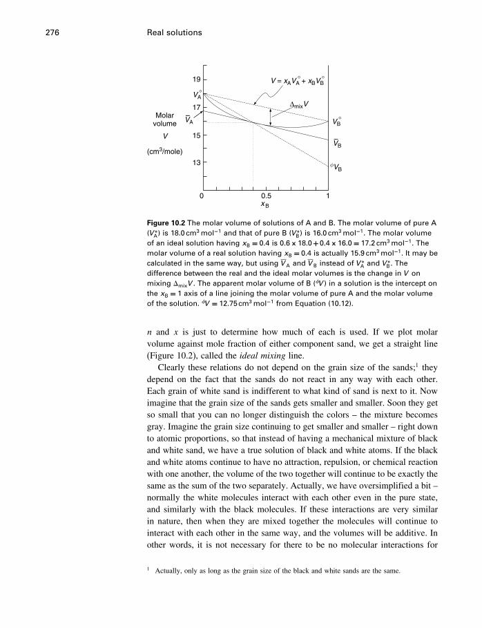
276 Real solutions
10
13
15
17
19
0.5
V = xAVA + xBVB
∆mixV
° °
φVB
VB°
VA°
Molarvolume
(cm3/mole)
VVB–
VA–
x B
Figure 10.2 The molar volume of solutions of A and B. The molar volume of pure A(V �
A) is 18.0 cm3 mol−1 and that of pure B (V �B) is 16.0 cm3 mol−1. The molar volume
of an ideal solution having xB = 0�4 is 0�6×18�0+0�4×16�0 = 17�2 cm3 mol−1. Themolar volume of a real solution having xB = 0�4 is actually 15.9 cm3 mol−1. It may becalculated in the same way, but using V A and V B instead of V �
A and V �B. The
difference between the real and the ideal molar volumes is the change in V onmixing �mixV . The apparent molar volume of B (�V ) in a solution is the intercept onthe xB = 1 axis of a line joining the molar volume of pure A and the molar volumeof the solution. �V = 12�75cm3 mol−1 from Equation (10.12).
n and x is just to determine how much of each is used. If we plot molarvolume against mole fraction of either component sand, we get a straight line(Figure 10.2), called the ideal mixing line.
Clearly these relations do not depend on the grain size of the sands;1 theydepend on the fact that the sands do not react in any way with each other.Each grain of white sand is indifferent to what kind of sand is next to it. Nowimagine that the grain size of the sands gets smaller and smaller. Soon they getso small that you can no longer distinguish the colors – the mixture becomesgray. Imagine the grain size continuing to get smaller and smaller – right downto atomic proportions, so that instead of having a mechanical mixture of blackand white sand, we have a true solution of black and white atoms. If the blackand white atoms continue to have no attraction, repulsion, or chemical reactionwith one another, the volume of the two together will continue to be exactly thesame as the sum of the two separately. Actually, we have oversimplified a bit –normally the white molecules interact with each other even in the pure state,and similarly with the black molecules. If these interactions are very similarin nature, then when they are mixed together the molecules will continue tointeract with each other in the same way, and the volumes will be additive. Inother words, it is not necessary for there to be no molecular interactions for
1 Actually, only as long as the grain size of the black and white sands are the same.
10.2 Solution volumes 277
ideal mixing, only that white molecules react with black molecules in exactlythe same way that they do with other white molecules.
But suppose that at this molecular size, white (w) and black (b) particles areattracted to one another more than to others of the same kind, perhaps evenforming a new kind of particle (wb). Because of this attraction, the particleswill be closer together than they would otherwise be, and the total volume ofthe mixture will be smaller, as shown in Figure 10.1b, and instead of gettinga straight mixing line as in Figure 10.2, the line is curved downward as inFigure 10.2. Alternatively, if the white and black particles repel each other,the total volume will be greater, and in Figure 10.2b the curved line for themolar volume of the mixture will lie above the straight line that represents nointeraction. The volume change on mixing (�mixV , Figure 10.2) caused by theattraction between A and B is the difference between the straight line and thecurved line. The straight line
V = xA V �A+xB V �
B (10.4)
is called ideal mixing and is rarely observed.2 The curved line representsnonideal mixing, the general case. The difference between the ideal mixingline and the actual molar volume V is called the change in volume on mixing,�mixV . Thus
�mixV = V − �xA V �A+xB V �
B� (10.5)
10.2.2 Partial molar volumes
Now suppose in our mixture of white and black particles that attract each other,that we are not satisfied to have the total volume or the molar volume of themixture as a whole. We would like to know the volume of each componentin the mixture, not just the combined volume. But how can this be done,when each is dispersed at the molecular level and is interacting strongly withanother component? Simple. Just draw the tangent to the molar volume curveat the composition you are interested in. The intercepts of this tangent givethe volumes of each component in the solution, called partial molar volumes,which are combined to give the total molar volume in exactly the same way asthe black and white sands in Equation (10.2) and Figure 10.2.
Looking at partial molar volumes in this way, they seem to be just a sort ofgeometrical construct. They are defined such that they can be substituted forVA and VB in Equation (10.2) in cases where mixing results in a curved linefor the molar volumes; thus3
V = xA VA+xB VB (Figure 10.2) (10.6)
2 Volumetric ideal mixing (Equation 10.4) is also called Amagat’s law, which we saw wasconnected to the Lewis fugacity rule in Chapter 8.
3 These equations are also derived in §C.2.3.
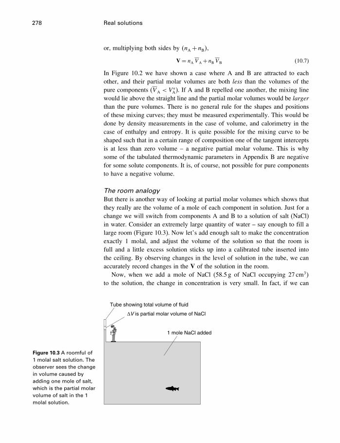
278 Real solutions
or, multiplying both sides by �nA+nB�,V= nA VA+nB VB (10.7)
In Figure 10.2 we have shown a case where A and B are attracted to eachother, and their partial molar volumes are both less than the volumes of thepure components (VA < V
�A). If A and B repelled one another, the mixing line
would lie above the straight line and the partial molar volumes would be largerthan the pure volumes. There is no general rule for the shapes and positionsof these mixing curves; they must be measured experimentally. This would bedone by density measurements in the case of volume, and calorimetry in thecase of enthalpy and entropy. It is quite possible for the mixing curve to beshaped such that in a certain range of composition one of the tangent interceptsis at less than zero volume – a negative partial molar volume. This is whysome of the tabulated thermodynamic parameters in Appendix B are negativefor some solute components. It is, of course, not possible for pure componentsto have a negative volume.
The room analogyBut there is another way of looking at partial molar volumes which shows thatthey really are the volume of a mole of each component in solution. Just for achange we will switch from components A and B to a solution of salt (NaCl)in water. Consider an extremely large quantity of water – say enough to fill alarge room (Figure 10.3). Now let’s add enough salt to make the concentrationexactly 1 molal, and adjust the volume of the solution so that the room isfull and a little excess solution sticks up into a calibrated tube inserted intothe ceiling. By observing changes in the level of solution in the tube, we canaccurately record changes in the V of the solution in the room.
Now, when we add a mole of NaCl (58.5 g of NaCl occupying 27 cm3�
to the solution, the change in concentration is very small. In fact, if we can
Figure 10.3 A roomful of1 molal salt solution. Theobserver sees the changein volume caused byadding one mole of salt,which is the partial molarvolume of salt in the 1molal solution.
Tube showing total volume of fluid
∆V is partial molar volume of NaCl
1 mole NaCl added
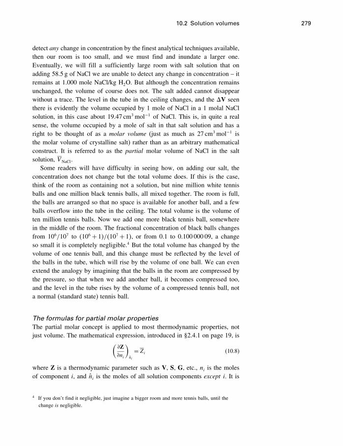
10.2 Solution volumes 279
detect any change in concentration by the finest analytical techniques available,then our room is too small, and we must find and inundate a larger one.Eventually, we will fill a sufficiently large room with salt solution that onadding 58.5 g of NaCl we are unable to detect any change in concentration – itremains at 1.000 mole NaCl/kg H2O. But although the concentration remainsunchanged, the volume of course does not. The salt added cannot disappearwithout a trace. The level in the tube in the ceiling changes, and the �V seenthere is evidently the volume occupied by 1 mole of NaCl in a 1 molal NaClsolution, in this case about 19.47 cm3 mol−1 of NaCl. This is, in quite a realsense, the volume occupied by a mole of salt in that salt solution and has aright to be thought of as a molar volume (just as much as 27 cm3 mol−1 isthe molar volume of crystalline salt) rather than as an arbitrary mathematicalconstruct. It is referred to as the partial molar volume of NaCl in the saltsolution, VNaCl.
Some readers will have difficulty in seeing how, on adding our salt, theconcentration does not change but the total volume does. If this is the case,think of the room as containing not a solution, but nine million white tennisballs and one million black tennis balls, all mixed together. The room is full,the balls are arranged so that no space is available for another ball, and a fewballs overflow into the tube in the ceiling. The total volume is the volume often million tennis balls. Now we add one more black tennis ball, somewherein the middle of the room. The fractional concentration of black balls changesfrom 106/107 to �106 + 1�/�107 + 1�, or from 0.1 to 0.100 000 09, a changeso small it is completely negligible.4 But the total volume has changed by thevolume of one tennis ball, and this change must be reflected by the level ofthe balls in the tube, which will rise by the volume of one ball. We can evenextend the analogy by imagining that the balls in the room are compressed bythe pressure, so that when we add another ball, it becomes compressed too,and the level in the tube rises by the volume of a compressed tennis ball, nota normal (standard state) tennis ball.
The formulas for partial molar propertiesThe partial molar concept is applied to most thermodynamic properties, notjust volume. The mathematical expression, introduced in §2.4.1 on page 19, is(
�Z�ni
)ni
= Zi (10.8)
where Z is a thermodynamic parameter such as V, S, G, etc., ni is the molesof component i, and ni is the moles of all solution components except i. It is
4 If you don’t find it negligible, just imagine a bigger room and more tennis balls, until thechange is negligible.
280 Real solutions
important to note that the derivative is taken of the total quantity, Z, not themolar property, Z. It is the change in the total volume of the solution in theroom that is measured, not the molar volume.
Put in this partial differential form, partial molar properties look somewhatobscure. However, it is important to have an intuitive grasp of their meaning,and you will be well advised to think of them in the sense of the room analogy,as molar properties of solutes in solutions of particular compositions, ratherthan in terms of Equation (10.8).
10.2.3 Apparent molar volume
The first thing we come across when looking at real data is that quite often thedata are reported as “apparent” molar volumes, enthalpies, entropies or heatcapacities. If we call component 1 the solvent (usually water in our cases),component 2 the solute (say, NaCl), Z and Z the total and molar forms of anyof these properties, then apparent molar properties are defined as
�Z = Z−n1Z�1
n2(10.9)
or, in the case of volume,
�V = V−n1V �1
n2(10.10)
where V �1 is the molar volume of the pure phase. Thus the apparent molar
volume is the volume that should be attributed to a mole of solute, if oneassumes that the solvent contributes the same volume it has in its pure state(Figure 10.2). Alternatively,
V= n1V �1 +n2�V (10.11)
or, dividing by �n1+n2�,V = x1V �
1 +x2 ·�V (10.12)
The apparent molar volume is known as accurately and as easily as the molarvolume or the total volume of a solution whose composition is known, whereasfinding the partial molar volume always involves some manipulation of theraw data (such as determining a tangent) and requires a knowledge of a rangeof compositions, not just a single one. Therefore measurement of the densityof a solution (§5.8.1) enables you to calculate V, the total volume of thesolution. Then because you know the molar volume of the pure solvent V �
1 ,Equation (10.10) gives you the apparent molar volume of the solute in thesolution you measured.
10.2 Solution volumes 281
To obtain partial molar volumes from measurements of apparent molarvolumes, differentiate Equation (10.11),(
�V�n2
)T�P�n1
= V 2 (10.13)
= n2(��V
�n2
)T�P�n1
+�V (10.14)
=m(��V
�m
)+�V if n1 = 55�51 (10.15)
so that evidently we need an equation to represent �V as a function of m, inorder to calculate ���V/�m�. For electrolytes, it is found that using
√m rather
than m gives a more linear plot, so that Equation (10.15) becomes
V 2 =m(��V
�m1/2
)(�m1/2
�m
)+�V
= 12m
1/2
(��V
�m1/2
)+�V (10.16)
Extrapolating values of �V back to m= 0 will therefore provide a value of V�2,
the partial molar volume at infinite dilution, which is the standard state value.
10.2.4 An example from NaCl–H2O
As an example of the various terms we have defined, consider the systemNaCl–H2O. This system differs from the system A–B in Figure 10.2 only inthe sense that A and B are completely miscible (they dissolve in each other inall proportions), while in NaCl–H2O water becomes saturated with NaCl at aconcentration which depends on P and T . This is 6.1 molal at 25 �C, 10.4 molalat 300 �C, so we can only look at concentrations below this value.
Partial molar volumeApparent molar volumes at concentrations up to 5 molal are shown inTable 10.1 and Figure 10.4. If the mass of solvent, water, is 1 kg, then n1is 1000/18�0154 = 55�51, and n2 is the NaCl molality, m. The volume of thepure solvent V �
1 is 18.068 cm3 mol−1, so measurements of the total volume ofthe solution V give molar volumes [from V/�55�51+m�] and apparent molarvolumes from Equation (10.11).
Apparent molar volumes �V can be converted into partial molar volumesin several ways. One way would be to actually do the operation illustratedin Figure 10.2, that is, construct the tangent to the molar volume curve, anddetermine the intercept on the xNaCl = 1 axis.5 The tangent at 3 molal is shown
5 The mole fractions in Table 10.1 and Figure 10.5 are calculated using � = 1 rather than � = 2as defined in Equation (7.2). Extrapolating a tangent to xNaCl = 1 using � = 2 results in a valueof 1
2VNaCl, and the diagram is less intuitive.
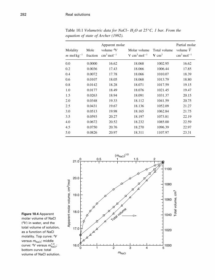
282 Real solutions
Table 10.1 Volumetric data for NaCl– H2O at 25 �C, 1 bar. From theequation of state of Archer (1992).
Apparent molar Partial molar
Molality Mole volume �V Molar volume Total volume volume V
m mol kg−1 fraction cm3 mol−1 V cm3 mol−1 V cm3 cm3 mol−1
0.0 0.0000 16.62 18.068 1002.95 16.62
0.2 0.0036 17.43 18.066 1006.44 17.85
0.4 0.0072 17.78 18.066 1010.07 18.39
0.6 0.0107 18.05 18.068 1013.79 18.80
0.8 0.0142 18.28 18.071 1017.59 19.15
1.0 0.0177 18.49 18.076 1021.45 19.47
1.5 0.0263 18.94 18.091 1031.37 20.15
2.0 0.0348 19.33 18.112 1041.59 20.75
2.5 0.0431 19.67 18.136 1052.09 21.27
3.0 0.0513 19.98 18.165 1062.84 21.75
3.5 0.0593 20.27 18.197 1073.81 22.19
4.0 0.0672 20.52 18.232 1085.00 22.59
4.5 0.0750 20.76 18.270 1096.39 22.97
5.0 0.0826 20.97 18.311 1107.97 23.31
mNaCl
(mNaCl)1/2
App
aren
t mol
ar v
olum
e, c
m3 /
mol
Tot
al v
olum
e, c
m3
0 1 2 3 4 5
0 0.5 1 1.5 2
16.0
17.0
18.0
19.0
20.0
21.0
1000
1020
1040
1060
1080
1100
Total volume
Figure 10.4 Apparentmolar volume of NaCl(�V ) in water, and thetotal volume of solution,as a function of NaClmolality. Top curve: �V
versus mNaCl; middlecurve: �V versus m
1/2NaCl;
bottom curve: totalvolume of NaCl solution.
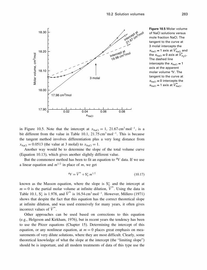
10.2 Solution volumes 283
x NaCl
Mol
ar v
olum
e, c
m3 /
mol
0 0.02 0.04 0.06 0.0817.90
18.00
18.10
18.20
18.30
intercept at
21.67 cm3 /m
ol
17.98 cm3/mol
3 molal
Intercept at
19.98 cm3 /mol
Figure 10.5 Molar volumeof NaCl solutions versusmole fraction NaCl. Thetangent to the curve at3 molal intercepts thexNaCl = 1 axis at V
�NaCl and
the xNaCl = 0 axis at V�H2O.
The dashed lineintercepts the xNaCl = 1axis at the apparentmolar volume �V . Thetangent to the curve atxNaCl = 0 intercepts thexNaCl = 1 axis at V
�NaCl.
in Figure 10.5. Note that the intercept at xNaCl = 1, 21.67 cm3 mol−1, is abit different from the value in Table 10.1, 21.75 cm3 mol−1. This is becausethe tangent method involves differentiation plus a very long distance fromxNaCl = 0�0513 (the value at 3 molal) to xNaCl = 1.
Another way would be to determine the slope of the total volume curve(Equation 10.13), which gives another slightly different value.
But the commonest method has been to fit an equation to �V data. If we usea linear equation and m1/2 in place of m, we get
�V = V�+S∗V m
1/2 (10.17)
known as the Masson equation, where the slope is S∗V and the intercept at
m = 0 is the partial molar volume at infinite dilution, V�. Using the data in
Table 10.1, S∗V is 1.978, and V
�is 16.54 cm3 mol−1. However, Millero (1971)
shows that despite the fact that this equation has the correct theoretical slopeat infinite dilution, and was used extensively for many years, it often givesincorrect values of V
�.
Other approaches can be used based on corrections to this equation(e.g., Helgeson and Kirkham, 1976), but in recent years the tendency has beento use the Pitzer equations (Chapter 15). Determining the intercept of thisequation, or any nonlinear equation, at m = 0 places great emphasis on mea-surements of very dilute solutions, where they are most difficult. Clearly, sometheoretical knowledge of what the slope at the intercept (the “limiting slope”)should be is important, and all modern treatments of data of this type use the
284 Real solutions
limiting slopes predicted from Debye–Hückel theory, which will be discussedin Chapter 15. The values in Table 10.1 from Archer (1992) are from an equa-tion of state which uses the theoretical limiting slopes, and in addition involvesnot just the data at 25 �C, 1 bar, but a great many other data as well.
ElectrostrictionMillero (1971) provides an interesting history of ideas on the volume occupiedby dissolved electrolytes. Before 1770, a salt was thought to dissolve in watersimply by filling up void spaces, thereby not changing the water volume. Theexperimental evidence used to support this idea was that a glass of water didnot overflow when a spoonful of salt was added. In 1770 Watson (referencein Millero, 1971) showed that the volume definitely decreases when varioussalts are added to water, showing that the prevailing theory of the “porous”nature of water was incorrect. However, his work was soon forgotten, and theolder ideas prevailed for another 70 years. Millero reports that Watson tired ofchemistry and entered the ministry.
These days we look at the partial molar volume of salts. The molar volumeof pure crystalline NaCl is 27.015 cm3 mol−1, so you see from the values of thepartial molar volume in Table 10.1 that NaCl occupies less volume per molein solution than it does in the solid form, at all concentrations. This fact iseven more striking if you look at the partial molar volume at infinite dilution athigh temperatures, as shown in Figure 10.6. At every pressure up to 1000 bars,VNaCl becomes negative, reaching almost −100 cm3 mol−1 at 300 �C, saturationvapor pressure (which is 86 bars). This means that if you were the observeron top of the room full of pure water in Figure 10.3, and if the water was at300 �C, you would observe the volume of water in the room to decrease byalmost 100 cm3 when 58 grams of NaCl was added to the water. The volumeof water is so large that after adding the salt, its presence is undetectable, i.e., itis at infinite dilution.
Figure 10.1 suggests that this effect is due to attraction between the NaCland the H2O. This is true, but in the case of electrolytes in water, it is somewhatoversimplified. Water is not gas-like, with a complete absence of structure,but largely due to its polar nature and hydrogen bonding, it has some kindof structure which has been the subject of much debate. Addition of chargedparticles in the form of a dissociated electrolyte disrupts and “collapses” thisstructure, and the resulting ion–water interactions of several types usuallyresults in an overall decrease in volume, known as “electrostriction”, despitethe additional volume of the electrolyte. These interactions form the basis ofthe HKF model embedded in supcrt92, to be discussed in Chapter 15.
10.3 The infinite dilution standard state
So far we have just assumed that the standard state for our mixing componentsis the pure phase, just as it was in Chapter 3. This presents no problem
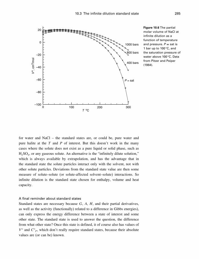
10.3 The infinite dilution standard state 285
T oC
Vo ,
cm
3 /m
ol
0 100 200 300–100
–80
–60
–40
–20
0
20
P = sat
400 bars
800 bars
1000 bars
Figure 10.6 The partialmolar volume of NaCl atinfinite dilution as afunction of temperatureand pressure. P = sat is1 bar up to 100 �C, andthe saturation pressure ofwater above 100 �C. Datafrom Pitzer and Peiper(1984).
for water and NaCl – the standard states are, or could be, pure water andpure halite at the T and P of interest. But this doesn’t work in the manycases where the solute does not exist as a pure liquid or solid phase, such asH2SO4, or any gaseous solute. An alternative is the “infinitely dilute solution,”which is always available by extrapolation, and has the advantage that inthe standard state the solute particles interact only with the solvent, not withother solute particles. Deviations from the standard state value are then somemeasure of solute–solute (or solute-affected solvent–solute) interactions. Soinfinite dilution is the standard state chosen for enthalpy, volume and heatcapacity.
A final reminder about standard states
Standard states are necessary because G, A, H , and their partial derivatives,as well as the activity (functionally) related to a difference in Gibbs energies),can only express the energy difference between a state of interest and someother state. The standard state is used to answer the question, the differencefrom what other state? Once this state is defined, it of course also has values ofV ° and C°P , which don’t really require standard states, because their absolutevalues are (or can be) known.
286 Real solutions
10.3.1 The entropy standard state
In summary, then, for dissolved substances we use the ideal one molal standardstate for Gibbs energy, and the infinite dilution standard state for enthalpy,volume and heat capacity. What about entropy?
By looking at one of our Equations (7.26)
�A−G�A = RT ln xA
it is easy to see why we cannot use infinite dilution for Gibbs energy. G�A is
a constant, so �A →−� as xA → 0. So infinite dilution is hard to deal with.Equation (7.28) is
Si−S�i =−R ln xi
so the same problem arises for entropy. Now we can write
G=H−TSG� =H� −TS�
and
G−G� = �H−H��−T�S−S��
where G� is for an ideal one molal solution and H� is for infinite dilution, andthe question is, to what does S� refer?
It happens that for H (and V , CP), the value at infinite dilution is equal tothe value in an ideal one molal solution (and anywhere else on the Henryantangent), so if G, H , and S refer to an ideal one molal solution, then G−G�
and H−H� are both zero, and S−S� is zero only if S� also refers to an idealone molal solution. Because entropy is calculated from other measurements(e.g., S = �H−G�/T ) rather than being measured directly, this fact is perhapsnot as useful as the others we have been discussing.
10.3.2 The reference state
Because partial molar volume, enthalpy, and heat capacity are the same any-where on the Henry’s law tangent, including both the state of infinite dilutionand the ideal one molal solution, either of these states can serve as the standardstate for these properties. We have chosen to say that the infinitely dilute solu-tion is the standard state, but many treatments prefer to say that the standardstate for these properties, as well as for the Gibbs energy and entropy, is theideal one molal solution. For some reason, these treatments (e.g., Klotz, 1964,p. 361) then define the “reference state” for enthalpy, volume and heat capacity
10.4 Excess properties 287
as the state of infinite dilution. This appears to have little usefulness, whateverstandard state definition is used.
If the standard state is defined as having a fixed pressure of 1 bar, thereference state is also sometimes referred to as a state reached from the standardstate by a change in pressure (Pitzer and Brewer, 1961, p. 249). Because in thistext we use a variable pressure standard state, we have no need of the referencestate in this sense either.
10.3.3 Symbols for the standard state
Superscript �, as in V �, indicates the standard state. Up to this point, this hasgenerally been synonymous with the pure state (pure solid, liquid, or gas), soone might get the impression that � indicates the pure phase. However, withsolutions, we must be more careful, because the pure phase is not always thestandard state.
In solutions, particularly electrolyte solutions, the standard state for thesolvent is always the pure phase (pure water), so that, for example, V �
1 refersto the molar volume of pure component 1, that is, pure water. For the solute,the standard state for most properties is, as just mentioned, the state of infinitedilution, so we could use V
�2 for the partial molar volume of the solute in the
standard state. However, this proves a bit confusing, so for clarity we introducesuperscript � to indicate the infinite dilution state (V
�2 ), and we understand that
this is also the standard state for most properties. This raises the question of whatsymbol to use for the solute in its pure state. The IUPAC recommends the useof ∗ for pure substances, but our examples involve only minerals so we will justuse the mineral name. Thus we use V halite for the molar volume of pure NaCl.
In the case of the Gibbs energy for aqueous solutes we saw (§8.2.3) that thestandard state is neither the pure phase nor the infinitely dilute state, and theusual � symbol is appropriate, as in G� and ��.
10.4 Excess properties
In this section we extend our discussion of solution volumes (§10.2) to otherproperties, and introduce the excess properties. The difference between theproperty (V , H , etc.) of a real solution, and what that property would be if thesolution was ideal, is called an excess property.
Thus, from Equations (7.9), (7.10), (7.11),
V ex = Vreal sol’n−Videal sol’n= Vreal sol’n−
∑i
xiV�i (10.18)
= �mixV (10.19)
288 Real solutions
and similarly
Hex = �mixH (10.20)
CPex = �mixCP (10.21)
For ideal solutions, these quantities are of course all zero (Equations 7.12,7.13, 7.14). They are also true for the total properties, so that for idealsolutions
Vex = 0 (10.22)
Hex = 0 (10.23)
CPex = 0 (10.24)
Relations between excess properties are the same as between their parentproperties. For example,(
�Gex
�P
)T
=(�Greal
�P
)−(�Gideal�P
)(10.25)
= Vreal−Videal (10.26)
= V ex (10.27)
so that in addition, (�Gex
�T
)P
=−Sex (10.28)(�Hex
�T
)P
= CPex (10.29)
and so on.The total excess enthalpy is also called the relative enthalpy, L, and is
related to the excess total Gibbs energy by
L=Hex
=Gex+T Sex
=Gex−T(�Gex
�T
)P�m
(10.30)
=−T 2
(�Gex/T
�T
)P�m
(10.31)
The total excess heat capacity, the relative heat capacity, also gets its ownsymbol
J= CPex (10.32)
=(�Hex
�T
)P�m
(10.33)
10.4 Excess properties 289
For entropy,
Sex = Sreal sol’n−Sideal sol’n (10.34)
= �mixSreal sol’n−�mixSideal sol’n
= �mixSreal sol’n+R∑i
xi ln xi (10.35)
Excess total entropy is also related to the relative enthalpy and excess totalGibbs energy as
Sex = �L−Gex�/T (10.36)
For Gibbs energy,
Gex =Greal sol’n−Gideal sol’n
= �mixGreal sol’n−�mixGideal sol’n
= �mixGreal sol’n−RT∑i
xi ln xi (10.37)
Partial molar excess propertiesThese have the same meaning as other partial molar properties. The generalformulation then is (
�Zex
�ni
)ni
= Zexi
=(�Zreal
�ni
)−(�Zideal
�ni
)
= Zreali −Zideal
i
For volume, using i= 2 to indicate the solute, this becomes
Vex2 = V real
2 −V ideal2
= V real2 −V�
2
superscript “real” is not generally needed, so we have
Vex2 = V 2−V�
2 (10.38)
where the substitution Videal2 = V�
2 means that we are using the infinitely dilutesolution of the solute as the ideal solution. It is therefore a Henryan sort ofideal solution. Similarly for enthalpy and heat capacity, the only differencebeing that they get special symbols,
Hex2 =H2−H�
2 (10.39)
= L2 (10.40)
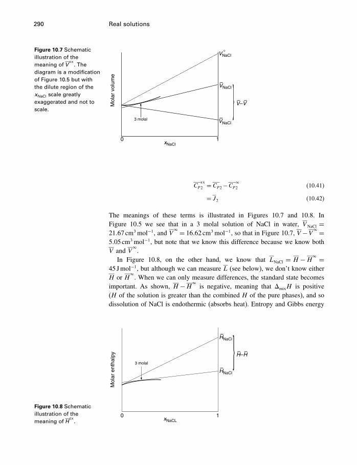
290 Real solutions
Figure 10.7 Schematicillustration of themeaning of V
ex. The
diagram is a modificationof Figure 10.5 but withthe dilute region of thexNaCl scale greatlyexaggerated and not toscale.
xNaCl10
Mol
ar v
olum
e
VNaCl°
VNaCl
VNaCl
V–V
–
–
–
–
3 molal
CPex2 = CP2−CP
�2 (10.41)
= J 2 (10.42)
The meanings of these terms is illustrated in Figures 10.7 and 10.8. InFigure 10.5 we see that in a 3 molal solution of NaCl in water, VNaCl =21�67cm3 mol−1, and V
� = 16�62 cm3 mol−1, so that in Figure 10.7, V −V� =5�05cm3 mol−1, but note that we know this difference because we know bothV and V
�.
In Figure 10.8, on the other hand, we know that LNaCl = H −H� =45 Jmol−1, but although we can measure L (see below), we don’t know eitherH or H
�. When we can only measure differences, the standard state becomes
important. As shown, H −H�is negative, meaning that �mixH is positive
(H of the solution is greater than the combined H of the pure phases), and sodissolution of NaCl is endothermic (absorbs heat). Entropy and Gibbs energy
Figure 10.8 Schematicillustration of themeaning of H
ex. xNaCL
10
Mol
ar e
ntha
lpy
HNaCl
H–H
–
–
HNaCl–
–
3 molal
10.4 Excess properties 291
on the other hand do not get special symbols.
Sex = S−Sideal (10.43)
and is not measured but calculated from other quantities, and
Gex = �ex
=G−Gideal
= �−�ideal (10.44)
But there are some important differences besides the lack of special symbols.
1. We write superscript � rather than � because the standard state for these quantities
is not the infinitely dilute solution, and it is not always the pure phase, and
2. Gibbs energy has a completely different functional relationship to concentration than
do the other properties. They all use the apparent properties, which we defined in
§10.2.3, whereas with Gibbs energy we use Equations (8.30).
For aqueous solutions, it is more useful to write
Gexi = �ex
i
= �i−�ideali
= ���i +RT ln �mii��− ���
i +RT lnmi�
= RT lni (10.45)
or
�exi
RT= lni (10.46)
or, as it often appears,
�Gex/RT
�ni= lni (10.47)
Another expression for excess Gibbs energiesThe molar Gibbs energy of ideal mixing was given as in Chapter 7 as
�mixGideal sol’n = RT∑i
xi ln xi [7.20]
It will be useful to have an expression for the Gibbs energy of mixing ofreal solutions. This is a bit more complicated for aqueous systems which are“unsymmetrical,” that is, which have different standard states for the solventand solute, and a completely different method of expressing deviations fromideality – osmotic coefficients for the solvent, and Henryan activity coefficientsfor the solutes. This development follows Pitzer (1991).
292 Real solutions
To start, think about Figure 7.4, but instead of ideal mixing, the mixing isfor a real case, and the curve has any shape. Whatever the shape of the mixingcurve, the chemical potentials of the two components are still given by thetangent intercepts, and the molar Gibbs energy of mixing of a real solution canbe expressed as
�mixG= xA��A−��A�+xB��B−��
B�
Because we will need excess chemical potentials as well, we change to thetotal form of the Gibbs energy (recall that chemical potentials are derivativesof the total Gibbs energy G, not of the molar Gibbs energy G). Multiplyingboth sides by �nA+nB�, we get
�mixG= nA��A−��A�+nB��B−��
B�
or, where component A is H2O and there are several solutes B,
�mixG= nH2O��H2O
−��H2O�+∑
i
ni��i−��i �
= RT(nH2O
lnaH2O+∑
i
ni lnai
)(10.48)
If the number of moles of water in a system is nH2O, the number of kilograms
of water is
kgw = nH2O
55�51
and for ni moles of solute i, ni/kgw is the number of moles of i per kg ofwater, i.e., the molality, mi. Substituting this relation, the relation ai = mii,and Equation (8.37)
�=− 55�51∑i mi
lnaH2O[8.37]
into (10.48), we get
�mixG= RT∑i
ni�−�+ ln �mii�� (10.49)
Next we divide this into an ideal part containing only concentration termsand another part containing the correction terms � and ,
�mixG=−RT∑i
ni�1− lnmi�︸ ︷︷ ︸ideal part
+RT∑i
ni�1−�+ lni�︸ ︷︷ ︸corrective part
The “corrective part” is evidently the excess Gibbs energy, so
Gex = �mixG+RT∑i
ni�1− lnmi� (10.50)
= RT∑i
ni�1−�+ lni�� (10.51)
10.5 Enthalpy and heat capacity 293
and
Gex/kgw = RT∑i
mi�1−�+ lni� (10.52)
and, as in (10.47) [�Gex/�kgwRT�
�mi
]nH2O
= lni (10.53)
[Pitzer 1973, Equation (23); 1991, Equation (34)] but now we also have anexpression for � in terms of Gex,
�−1=− ��Gex/�kgw�niRT∑i mi
(10.54)
[Pitzer 1973, Equation (22); 1991, Equation (35)].Because Gibbs energy as a function of T and P is a fundamental equation
(§4.12.1), excess Gibbs energies can be used to calculate not only activitycoefficients but all other deviations from ideal behavior, such as osmotic coef-ficients, excess enthalpies, excess heat capacities, excess volumes, and so on(§10.4), so it is potentially quite informative. Also, properties calculated fromGex in this way will be entirely self-consistent, which might not be the case ifeach property was determined separately.
However, determiningGex for multicomponent electrolyte aqueous solutionshas proved to be a difficult task. Virtually all applications these days use theformulation of K.S. Pitzer and his colleagues, developed during the 1970s and1980s, which we discuss in Chapter 15. Equation (10.52) and its derivativesare the essential first step in the development of the Pitzer equations.
10.5 Enthalpy and heat capacity
Starting with Equation (10.7) as applied to enthalpy rather than volume, andadopting the usual convention where component 1 is the solvent and compo-nent 2 the solute,6
H= n1H1+n2H2 (10.55)
where the partial molar enthalpies are of course
H1 =(�H�n1
)T�P�n2
H2 =(�H�n2
)T�P�n1
6 Equation (10.55) is self-evident to someone familiar with Euler’s theorem (§C.2.3).
294 Real solutions
And, as with the other partial molar properties (except �), it is convenient touse apparent properties, so from Equation (10.9),
�H2 =H−n1H�
1
n2(10.56)
and
�H�2 = H�−n1H�
1
n2(10.57)
where H�1 is the molar enthalpy of pure water. As before, the apparent and
partial molar enthalpies are related by
H2 = n2(��H2
�n2
)T�P�n1
+�H2 (10.58)
Equation (10.55) remains true as n2 → 0, so we can write
H� = n1H�1 +n2H�
2
= n1H�1 +n2H�
2 (10.59)
where we can write H�1 in place of H
�1 because infinitely dilute component 1
is just pure water, and partial molar properties are the same as molar propertiesfor pure phases.
Subtracting (10.59) from (10.55),
H−H� = n1�H1−H�1 �+n2�H2−H�
2 � (10.60)
= n2��H2−�H�2 � (10.61)
Now if we define
L=H−H� (10.62)
L1 =H1−H�1 (10.63)
L2 =H2−H�2 (10.64)
�L2 = �H2−�H�2 (10.65)
we have
L= n1 L1+n2 L2 (10.66)
= n2�L2� (10.67)
so
�L2 =Ln2
(10.68)
10.5 Enthalpy and heat capacity 295
where L is called the relative enthalpy of the solution, L2 is the relative partialmolar enthalpy and �L2 is the apparent relative molar enthalpy of component 2.Equation (10.66) is clearly analogous to (10.7) and (10.55). At infinite dilution,both L1 and L2 are zero. Equation (10.62) can also be written
L=H−H�1
=H−n1H�1 (10.69)
In other words L is the difference between the total enthalpy of a solutionand the total enthalpy of the same amount of pure water. Differentiating Equa-tion (10.67) with respect to n2 we get a familiar expression for L2,
L2 =�L�n2
= n2(��L2
�n2
)T�P�n1
+�L2 (10.70)
and, as with volume, using√m is often advantageous, so Equation (10.70)
becomes
L2 = 12m
1/2
(��L2
�m1/2
)+�L2 (10.71)
An expression for L1 can be obtained by substituting Equations (10.70) and(10.67) into (10.66),
n1L1 = n2�L2−n2L2
= n2�L2−n2[�L2+n2
(��L2
�n2
)n1
]
L1 =−n22
n1
(��L2
�n2
)(10.72)
Values of L2 can be obtained by measuring heats of dilution. The meaning ofsome of these terms is illustrated in Figure 10.9.
10.5.1 Heat of dilution
When a solution of initial molality mi is diluted to a final molality mf , theobserved heat effect is
�dilutionH = �L2�mf �−�L2�mi�
= ��L2 (10.73)
which, if you insert the definitions of �L2, and�H2, means that
�dilutionH = Hf −Hi
n2
296 Real solutions
Figure 10.9 Schematicillustration of themeaning of someenthalpy terms. H2
H2
Hhalite L2
L2
Differential heat
of solution
Mol
ar e
ntha
lpy,
H
Figure 10.10 The heat ofdilution of NaCl from1 molal to the finalmolality shown, at theindicated temperatures.Data from Busey et al.(1984).
++ ++ ++ +++++ +++
++
++
+
+
+
++
+
Final molality
Hea
t of
dilu
tion,
Jm
ol–1
0 0.1 0.2 0.3 0.4 0.5 0.6 0.7 0.8
–20000
–15000
–10000
–5000
0
Initial molality = 1.0
372.85 K
473.05 K
572.85 K
or, if you prefer,
�dilutionH=Hf −Hi (10.74)
Some experimental heat of dilution data for NaCl are shown in Figure 10.10.The negative values show that the enthalpy of a dilute NaCl solution is lessthan that of a more concentrated one. The data in this diagram are an answerto the question “what is the (nonideal) heat of mixing of NaCl and water?” Inthis case the NaCl is at two different concentrations – one is 1.0 molal, and theother is as shown on the x-axis.
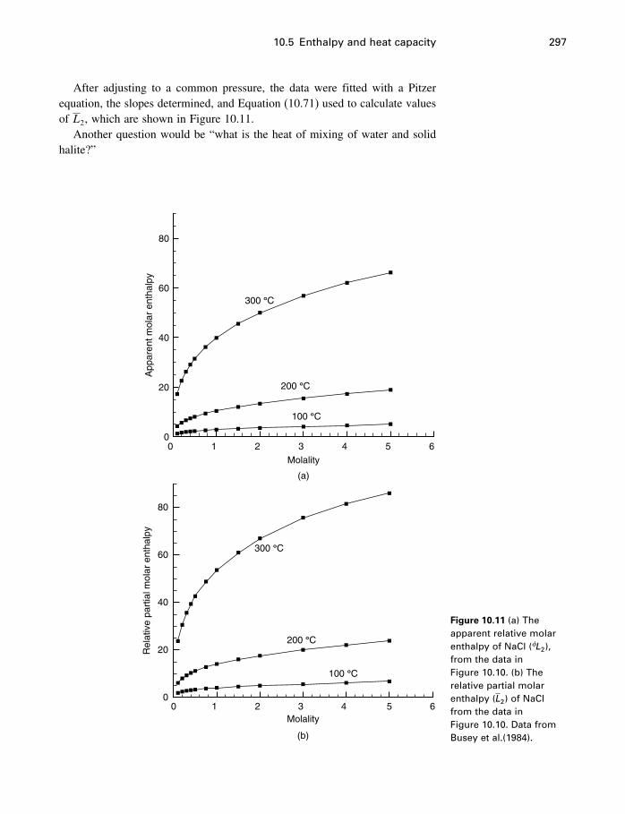
10.5 Enthalpy and heat capacity 297
After adjusting to a common pressure, the data were fitted with a Pitzerequation, the slopes determined, and Equation (10.71) used to calculate valuesof L2, which are shown in Figure 10.11.
Another question would be “what is the heat of mixing of water and solidhalite?”
Molality
Rel
ativ
e pa
rtia
l mol
ar e
ntha
lpy
0 1 2 3 4 5 60
20
40
60
80
Molality
App
aren
t mol
ar e
ntha
lpy
0 1 2 3 4 5 60
20
40
60
80
300 °C
200 °C
100 °C
300 °C
200 °C
100 °C
(b)
(a)
Figure 10.11 (a) Theapparent relative molarenthalpy of NaCl (�L2),from the data inFigure 10.10. (b) Therelative partial molarenthalpy (L2) of NaClfrom the data inFigure 10.10. Data fromBusey et al.(1984).
298 Real solutions
10.5.2 Integral heat of solution
The dissolution of halite in water can be written as
n2 NaCl�s�+n1 H2O�l�= �solution of n2 moles of NaCl and n1 moles of H2O�
(10.75)
or alternatively
n2 NaCl�s�+55�51H2O�l�= n2 NaCl�aq�m� (10.76)
where �aq�m� signifies an aqueous solution of concentration m.This process of forming a solution from pure solvent and pure solute is
called the integral heat of solution, and the heat effect in this process is
�integralH= �mixH
= �n1H1+n2H2�︸ ︷︷ ︸H solution
− �n1H�1 +n2Hhalite�︸ ︷︷ ︸
H pure phases
= n1�H1−H�1 �+n2�H2−Hhalite� (10.77)
= n1L1+n2�H2−H�2 �−n2�Hhalite−H�
2 �
= n1L1+n2L2︸ ︷︷ ︸L
−n2�Hhalite−H�2 � (10.78)
where �n1H1 + n2H2� is the absolute enthalpy of the solution itself (Equa-tion 10.55), Hsolution, and �n1H
�1 +n2Hhalite� is the absolute enthalpy of the pure
starting materials, water and Halite. It is actually a form of Equation (7.13),except that we write Hsolution and mole numbers rather than H ideal sol’n and molefractions, and it is a form of Equation (10.60) but using a different standard statefor component 2. Many sources introduce another symbol for �Hhalite −H�
2 �,such as L
halite, or L�s�, but we will retain �Hhalite−H�
2 � in a small and perhapsfutile attempt to lessen confusion.
Integral heats of solution cannot be obtained directly from heat of dilutionmeasurements, because they do not include the energy required to break thesolid into its constituent ions, and then hydrate them. This is shown by the factthat a term for Hhalite appears in our equations.
Dividing through by n2 in Equation (10.78) we get a more intuitive expres-sion for the integral heat of solution:
�integralH
n2= Ln2
− �Hhalite−H�2 ��
or
�integralH = �L2+ �H�2 −Hhalite� (10.79)
10.5 Enthalpy and heat capacity 299
In this equation �H�2 −Hhalite� is the heat of solution of halite into an infinite
amount of water, and �L2is the heat difference between this infinitely dilutesolution (which is pure water) and the solution at whatever concentration wewish. When the concentration of interest is 1 molal, �L2 is given by the interceptof the curves in Figure 10.10 at m= 0, and because �L2 at infinite dilution iszero, it is shown for all concentrations in Figure 10.11a.
10.5.3 Differential heat of solution
The differential heat of solution is another name for the partial molar enthalpy ofsolution, i.e., the heat effect of dissolving a mole of solute in an infinite amountof solution of some particular concentration. It’s like measuring the heat effectinstead of the volume effect in Figure 10.3, and it’s just the slope of the integralheat effect. The integral and differential heats of solution become identicalat infinite dilution. According to the definition of partial molar properties(Equation 10.8), differentiation of an equation for the integral heat should giveus the differential heat, so(
��integralH
�n2
)T�P�n1
=(�L�n2
)T�P�n1
+(� n2�H
halite−H�2 �
�n2
)T�P�n1
= L2+ �Hhalite−H�2 � (10.81)
=H2−Hhalite (10.82)
Klotz (1964, p. 291) gives the following expression for the heat absorbed(in calmol−1) when m moles of halite are dissolved in 1000 g of H2O (theintegral heat of solution of halite in water) at 25 �C
�integralH = 923m+476�1m3/2−726�1m2+243�5m5/2 (10.83)
so the differential heat is(��integralH
�m
)T�P
= 923+714�15m1/2−1452�2m+608�75m3/2 (10.84)
10.5.4 Heat capacity
Heat capacities can be measured directly in twin tube flow calorimeters (§5.8.2)or by manipulation of other measurements. For example, Criss and Cobble(1961) and Gardner, Mitchell and Cobble (1969) measured the heat of solu-tion of halite in water at various temperatures, extrapolated to standard stateconditions (infinite dilution), then determined the temperature derivative of the
300 Real solutions
Integral heat of solution of NaCl
How much heat is absorbed (or evolved?) when 1 mole of halite is dissolved in
1 kg of water at 100, 150, and 200 �C?
To calculate this we need to know
1. the enthalpy change when a mole of halite is dissolved in an infinite amount
of water, and
2. the enthalpy change between this solution and the 1 molal solution, which is
the negative of the heat of dilution from 1m to infinite dilution.
This is summed up in Equation (10.79).
Criss and Cobble (1961, 0–95 �C) and Gardner et al. (1961, 100–200 �C) reportvalues of the heat of solution of halite in dilute NaCl solutions, extrapolated to
mNaCl = 0, thus giving values of H�2 −Hhalite. If we combine these data we find
they are fit very well by a cubic polynomial, which is
H�2 −Hhalite = 1833�66−38�8870T +0�0161221T 2−0�000803184T 3 (10.80)
where T is in �C.
From the tabulated values in Busey et al. (1984) which were used to plot
Figure 10.11a, we find values of �LNaCl. Combining these data we get
T H�2 −Hhalite �LNaCl �integralH
°C Jmol−1 Jmol−1 Jmol−1
25 +914 ⇐ from Criss and Cobble (1960)
100 −5213 2861 −2352
150 −12898 5731 −7167
200 −24771 10400 −14371
The remarkable decrease in both H�2 −Hhalite and �integralH with temperature,
including a change from endothermic to exothermic in H�2 −Hhalite between
25 and 100 �C, is but one of many indications that there is a great increase in
energy liberating processes (hydration, solvent collapse, ion-pair formation) as T
is increased.
heat of solution measurements. At infinite dilution, because H1 = H�1 , Equa-
tion (10.77) becomes
�integralH= n2�H�2 −Hhalite�
or
�integralH = �H�2 −Hhalite� (10.85)
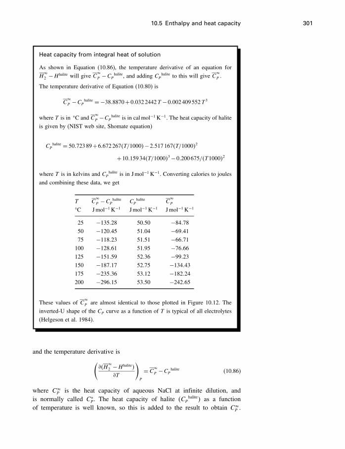
10.5 Enthalpy and heat capacity 301
Heat capacity from integral heat of solution
As shown in Equation (10.86), the temperature derivative of an equation for
H�2 −Hhalite will give C
�P −CP
halite, and adding CPhalite to this will give C
�P .
The temperature derivative of Equation (10.80) is
C�P −CP
halite =−38�8870+0�0322442T −0�002409552T 3
where T is in �C and C�P −CP
halite is in calmol−1 K−1. The heat capacity of halite
is given by (NIST web site, Shomate equation)
CPhalite = 50�72389+6�672267�T/1000�−2�517167�T/1000�2
+10�15934�T/1000�3−0�200675/�T1000�2
where T is in kelvins and CPhalite is in Jmol−1 K−1. Converting calories to joules
and combining these data, we get
T C�P −CP
halite CPhalite C
�P
°C Jmol−1 K−1 Jmol−1 K−1 Jmol−1 K−1
25 −135�28 50.50 −84�78
50 −120�45 51.04 −69�41
75 −118�23 51.51 −66�71
100 −128�61 51.95 −76�66
125 −151�59 52.36 −99�23
150 −187�17 52.75 −134�43
175 −235�36 53.12 −182�24
200 −296�15 53.50 −242�65
These values of C�P are almost identical to those plotted in Figure 10.12. The
inverted-U shape of the CP curve as a function of T is typical of all electrolytes
(Helgeson et al. 1984).
and the temperature derivative is(��H
�2 −Hhalite�
�T
)P
= C�P −CP
halite (10.86)
where C�P is the heat capacity of aqueous NaCl at infinite dilution, and
is normally called C�P. The heat capacity of halite �CP
halite� as a functionof temperature is well known, so this is added to the result to obtain C�
P .
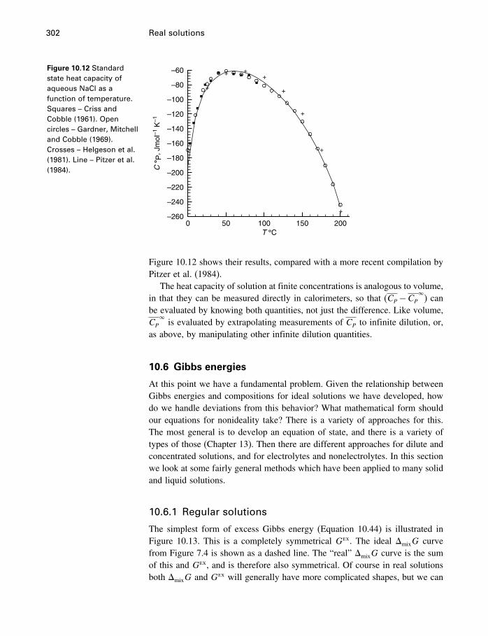
302 Real solutions
Figure 10.12 Standardstate heat capacity ofaqueous NaCl as afunction of temperature.Squares – Criss andCobble (1961). Opencircles – Gardner, Mitchelland Cobble (1969).Crosses – Helgeson et al.(1981). Line – Pitzer et al.(1984).
+
+ ++
+
+
+
+
T °C
C° P
, Jm
ol–1
K–1
0 50 100 150 200–260
–240
–220
–200
–180
–160
–140
–120
–100
–80
–60
Figure 10.12 shows their results, compared with a more recent compilation byPitzer et al. (1984).
The heat capacity of solution at finite concentrations is analogous to volume,in that they can be measured directly in calorimeters, so that (CP −CP
�) can
be evaluated by knowing both quantities, not just the difference. Like volume,CP
�is evaluated by extrapolating measurements of CP to infinite dilution, or,
as above, by manipulating other infinite dilution quantities.
10.6 Gibbs energies
At this point we have a fundamental problem. Given the relationship betweenGibbs energies and compositions for ideal solutions we have developed, howdo we handle deviations from this behavior? What mathematical form shouldour equations for nonideality take? There is a variety of approaches for this.The most general is to develop an equation of state, and there is a variety oftypes of those (Chapter 13). Then there are different approaches for dilute andconcentrated solutions, and for electrolytes and nonelectrolytes. In this sectionwe look at some fairly general methods which have been applied to many solidand liquid solutions.
10.6.1 Regular solutions
The simplest form of excess Gibbs energy (Equation 10.44) is illustrated inFigure 10.13. This is a completely symmetrical Gex. The ideal �mixG curvefrom Figure 7.4 is shown as a dashed line. The “real” �mixG curve is the sumof this and Gex, and is therefore also symmetrical. Of course in real solutionsboth �mixG and Gex will generally have more complicated shapes, but we can
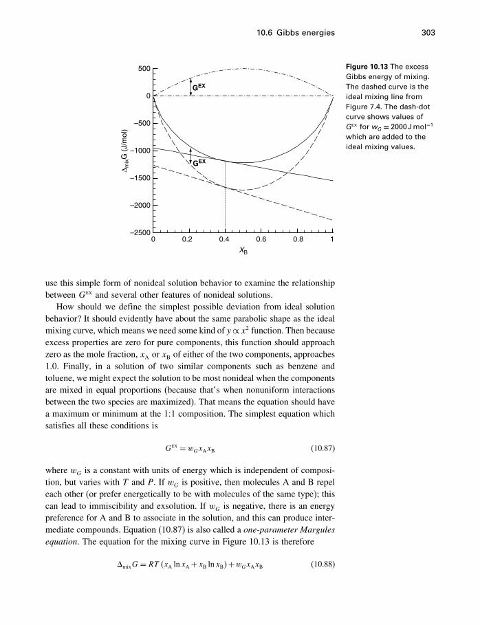
10.6 Gibbs energies 303
XB
∆ mixG
(J/
mol
)
0 0.2 0.4 0.6 0.8 1–2500
–2000
–1500
–1000
–500
0
500
GEX
GEX
Figure 10.13 The excessGibbs energy of mixing.The dashed curve is theideal mixing line fromFigure 7.4. The dash-dotcurve shows values ofGex for wG = 2000Jmol−1
which are added to theideal mixing values.
use this simple form of nonideal solution behavior to examine the relationshipbetween Gex and several other features of nonideal solutions.
How should we define the simplest possible deviation from ideal solutionbehavior? It should evidently have about the same parabolic shape as the idealmixing curve, which means we need some kind of y∝ x2 function. Then becauseexcess properties are zero for pure components, this function should approachzero as the mole fraction, xA or xB of either of the two components, approaches1.0. Finally, in a solution of two similar components such as benzene andtoluene, we might expect the solution to be most nonideal when the componentsare mixed in equal proportions (because that’s when nonuniform interactionsbetween the two species are maximized). That means the equation should havea maximum or minimum at the 1:1 composition. The simplest equation whichsatisfies all these conditions is
Gex = wGxAxB (10.87)
where wG is a constant with units of energy which is independent of composi-tion, but varies with T and P. If wG is positive, then molecules A and B repeleach other (or prefer energetically to be with molecules of the same type); thiscan lead to immiscibility and exsolution. If wG is negative, there is an energypreference for A and B to associate in the solution, and this can produce inter-mediate compounds. Equation (10.87) is also called a one-parameter Margulesequation. The equation for the mixing curve in Figure 10.13 is therefore
�mixG= RT �xA ln xA+xB ln xB�+wGxAxB (10.88)
304 Real solutions
Hildebrand and Scott (1964) discuss many (mostly binary) systems whichcan be conveniently treated with this formalism. It has been applied to ternarysystems, but beyond that it gets quite cumbersome. Although not many real sys-tems show such behavior (examples are systems like argon–oxygen, benzene–cyclohexane, Au–Cu), we can easily imagine adding more terms involving
Solution theories
There are literally thousands of articles on the theory of solutions, going back
to the origins of physical chemistry itself, yet, as pointed out by Prausnitz et al.
(1999, Chapter 7) after an extensive survey of the subject, “…we are still far
from an adequate theory of liquid mixtures.” Traditionally, and for good reason,
theories on electrolyte and nonelectrolyte solutions are treated separately, but
there is of course some common ground such as the laws of Raoult and Henry.
Theories of the two types of solutions also have an interesting similarity in that
they have generally been developed emphasizing either the “physical” or the
“chemical” approach.
In nonelectrolyte theory, the physical approach goes back to van der Waals,
and develops theories which deal with particle arrangements and generalized
intermolecular forces, but nothing about the specific nature of any new particles
formed due to these forces. The chemical approach concentrates on identifying
these new particles, and in the extreme form, begun by Dolezalek in 1908,
suggests that if all molecular species are correctly identified, with their respective
equilibrium constants, Raoultian mixing is sufficient to account for the solution
properties. The physical approach can be traced from van der Waals through van
Laar, Scatchard and Hildebrand, resulting in regular solution theory (references
in Prausnitz et al., 1999), which turns out to have some overlap with the equations
proposed by Margules in 1895.
In electrolyte theory, so different in most respects because of the electrically
charged nature of the particles, the same distinction between physical and chem-
ical approaches can be seen. We will present more detail in Chapter 15, but
basically the Pitzer equations represent the physical approach, having no reference
to individual ionic species, and the HKF model of Helgeson et al. (1981) repre-
sents the chemical approach, in which the standard state properties of individual
species are defined.
Modern theories of solutions combine aspects of both approaches, and the theories
of Pitzer and Helgeson et al. are no different in this respect. The Pitzer approach
must take into account strong complex formation, and the HKF approach uses
activity coefficients, based on generalized electrostatic considerations, in addition
to species information.
10.6 Gibbs energies 305
adjustable constants and mole fractions to account for more complex nonide-ality, and this approach has in fact been pursued extensively.
In Figure 10.13 we have assumed wG = 2000 Jmol−1, so that at xB = 0�4,wGxAxB = 480�0 Jmol−1, and �mixG from Equation (10.88) is −1668�4+480�0=−1188�4 Jmol−1.
Corrections to �H and �SBecause �G= �H−T�S, applying a correction to �G raises the question asto how this correction is divided between �H and �S. The two extreme caseswould be
1. that it all appears as a correction to �H with �S remaining ideal, or
2. it all appears as a correction to �S, with �H remaining zero
and, of course, there could be some adjustment in both terms. The originaldefinition of regular solutions by Hildebrand in 1927 was case 1, with an idealentropy of mixing and a nonideal enthalpy of mixing. The other case, retaining�H = 0, produces athermal solutions. Many other descriptive terms have beenused by other authors, and the term “regular solution” now covers both thesecases, as well as some extensions.
Because Gex =Hex−TSex, then
Sex =− �Gex
�T
=− �
�T�wG xAxB�
= xAxBwS (10.89)
where ��wG/�T�=−wS , and Hex is
Hex =Gex+T Sex
= xAxB�wG+T wS�= xAxBwH (10.90)
Similarly, ��wG/�P�= wV , V ex = xAxBwV , and
wG = wH −TwS+PwV (10.91)
Measurements of any of these excess quantities could then contribute to aknowledge of a system’s nonideality as a function of T and P. We give someexamples of how this is done in Chapter 14.
306 Real solutions
�−�� from tangentThe slope of the tangent to the mixing curve is(
d�mixG
dxB
)= d
dxB�RT �xA ln xA+xB ln xB�+wGxAxB�
= RT ln(xBxA
)+wG �1−2xB� (10.92)
and the equation for the tangent line itself is, as before,
�A = �mixG−xB(d�mixG
dxB
)(10.93)
Calculating the intercept on the xA axis of the tangent at xB = 0�4 with theseequations, we get �−�� = −946 Jmol−1.
�−�� from equationSubstitution of Equation (10.92) into Equation (10.93), remembering that �mixG
is now Equation (10.88), we find that
�A = RT ln xA+wGx2B
but we know that here �A is really �A−��, because we have implicitly assumedthat �� = 0. In other words, the intercept we calculated is the numerical valueon the xB axis, but that numerical value is a �G of mixing, a difference, soour �A is also a difference. What we have calculated is in fact
�A−��A = RT ln xA+wGx2B (10.94)
and at xA = 0�6, xB = 0�4, wG = 2000 Jmol−1, Equation (10.94) gives �A −��
A =−946 Jmol−1, in agreement (of course) with the tangent method.If in Equation (7.34) we change �i to �
idealA , and we compare this with
Equation (10.94), we see that
�A−�idealA = �ex
= wGx2B (10.95)
= 2000× �0�4�2
= 320 Jmol−1 (10.96)
=−946+1266 Jmol−1 (1266 is RT ln xA from page 195)
�−�� from activity coefficientAlso, it proves very convenient to define a correction factor for the molefraction term in Equation (7.34), such that the nonideal effects are taken intoaccount. In other words, instead of correcting the �G or �−�� side of the
10.6 Gibbs energies 307
equation withGex, we correct the mole fraction on the other side of the equationto give the same effect (we looked at this approach in more detail in Chapter 8).So we define a factor R such that
�A−��A = RT ln �xARA � (10.97)
= RT ln xA+RT lnRA
and comparing this with Equation (10.94) we see that
RT lnRA = wGx2BRT lnRB = wGx2A
⎫⎬⎭ (10.98)
At xB = 0�4 and wG = 2000 Jmol−1, RA= 1�1378 and �A − ��
A = RT
ln�0�6×1�1378�= 946 Jmol−1 again.So there is complete equivalence between the use of the activity coefficient
and the excess Gibbs energy. In a sense there is hardly any difference at all.If the correction for nonideality is in a logarithmic form (RT ln) it can becombined with the ideal term (RT ln x) as a correction to x. If it does not havea logarithmic form (wx2) it becomes a correction to the �G or �� term.
CO2 solubility in NaCl solutionsAn interesting application of regular solution theory is presented by Nesbitt(1984). He shows that activity coefficients for CO2 in aqueous NaCl solutionsto quite high temperatures (≈ 500 �C) and NaCl concentrations (≈ 6m) canbe fit very well by a slight modification of (10.98). As written, the activitycoefficients in (10.98) are based on Raoultian activities; that is, B → 1 asxB → 1. Solubility studies on the other hand normally use Henryan coefficients,where B → 1 as mB → 0, where mB is the molality of the solute.
Following Robinson and Stokes (1965), Nesbitt plots lnCO2versus
−�x22−1� instead of x22, where x2 is the mole fraction of H2O in the system.This has the desired effect of having CO2
→ 1 as x2 → 0. Nesbitt calculatesvalues of wG and discusses applications to boiling hydrothermal solutions.
UnmixingAs wG becomes larger, the mixing curve develops a flat portion, and eventuallysplits into two separate parabolic curves, one on each side of the diagram, asshown in Figure 10.14. In a real system this means that “unmixing” occurs.Instead of one homogeneous solution, two solutions form at equilibrium, thecompositions of which are at the minima in the mixing curve. The chemicalpotentials in each of the two solutions are given by the tangent common to thetwo minima, showing that �A and �B are the same in each solution. Generally,the two compositions converge as temperature increases, generating a solvus(a subject continued in Chapter 17). The mixing curve and the solvus arenot usually symmetrical as in this simple model. Somewhat more complexequations are required to generate asymmetry (§10.7).
308 Real solutions
Figure 10.14 The excessGibbs energy of mixingwith various values of wG,showing unmixing intotwo separate solutionswhen wG = 8000Jmol−1.The dashed line is atangent common to bothminima in this curve.
∆ mix
G
0 0.2 0.4 0.6 0.8 1–2000
–1500
–1000
–500
0
500
–2000
–1500
–1000
–500
0
500
Ideal
w = 3000
w = 5000
w = 8000 J/mol
Tangent
XB
Figure 10.15 The activitiesof A and B as a functionof xB fromEquations (10.98), withwG = 2000Jmol−1. Thesame data are shown inFigure 8.2.
XB
Act
ivity
0.0 0.2 0.4 0.6 0.8 1.00.0
0.1
0.2
0.3
0.4
0.5
0.6
0.7
0.8
0.9
1.0
aB
aA0.5348
R’s law
R’s law
10.6.2 The Raoultian activity
The activities of A (aA = xARA) and B (aB = xBRB
) as a function ofmole fraction are shown in Figure 10.15 and Table 10.2. At xB = 0�4 andwG = 2000 Jmol−1, RB
= 1�337 (Equation 10.98), so the activity of B is0�4×1�337= 0�5348, as shown.
10.6 Gibbs energies 309
The Margules equations
Margules (1895) suggested an equation for the vapor pressures of solution com-
ponents (partial pressures) in the form of a series expansion, using the systems
ethyl alchohol–water and methyl alchohol–water as examples. Using our notation,
his equation was
Pi = P�i x
0i e
�1�1−xi�+ 22 �1−xi�2+
33 �1−xi�3+··· � (10.99)
where i is 1 or 2 (binary solutions, so x2 = 1−x1), and where, to have the limiting
condition that Henry’s law is followed as x2 → 0, 0 = 1, and 1 = 0. This gives,
as �1−x1�→ 0,
Pi = P�i xi�
or
Pi = constant ·xiwhich is Henry’s law (§7.4.2).
If we assume that the partial pressures are in fact fugacities (fi = Pi), then using
ai = fi/f �ilni = ln
aixi
=n∑j=2
1j�j�1−xi�j� (10.100)
which, for a binary solution and n= 3, is
ln1 = 122 x
22 + 1
33 x32�
and so
RT ln1 = constant1 ·x22 + constant2 ·x32which is the same in form as Equations (10.105) or (10.107), and if truncated
to the first term on the right, is the same as the regular solution expression,
Equations (10.98).
There is an extensive literature in both chemistry and geochemistry on these and
other similar equations and their interrelations. Useful guides are Grover (1977)
and Thompson (1967). They apply to any solutions, solid, liquid, or gaseous.
Thompson points out that the Margules equations bear the same relationship to
Henry’s law that the virial equation (§13.5) has to the ideal gas law, in that the
first term in the virial series (in the form of 13.26) is the ideal gas law, and the
Margules equation condenses to Henry’s law, as shown above.
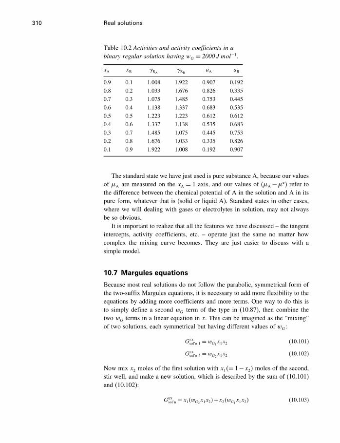
310 Real solutions
Table 10.2 Activities and activity coefficients in abinary regular solution having wG = 2000 J mol−1.
xA xB RARB
aA aB
0.9 0.1 1.008 1.922 0.907 0.192
0.8 0.2 1.033 1.676 0.826 0.335
0.7 0.3 1.075 1.485 0.753 0.445
0.6 0.4 1.138 1.337 0.683 0.535
0.5 0.5 1.223 1.223 0.612 0.612
0.4 0.6 1.337 1.138 0.535 0.683
0.3 0.7 1.485 1.075 0.445 0.753
0.2 0.8 1.676 1.033 0.335 0.826
0.1 0.9 1.922 1.008 0.192 0.907
The standard state we have just used is pure substance A, because our valuesof �A are measured on the xA = 1 axis, and our values of (�A −��) refer tothe difference between the chemical potential of A in the solution and A in itspure form, whatever that is (solid or liquid A). Standard states in other cases,where we will dealing with gases or electrolytes in solution, may not alwaysbe so obvious.
It is important to realize that all the features we have discussed – the tangentintercepts, activity coefficients, etc. – operate just the same no matter howcomplex the mixing curve becomes. They are just easier to discuss with asimple model.
10.7 Margules equations
Because most real solutions do not follow the parabolic, symmetrical form ofthe two-suffix Margules equations, it is necessary to add more flexibility to theequations by adding more coefficients and more terms. One way to do this isto simply define a second wG term of the type in (10.87), then combine thetwo wG terms in a linear equation in x. This can be imagined as the “mixing”of two solutions, each symmetrical but having different values of wG:
Gexsol’n 1 = wG1
x1x2 (10.101)
Gexsol’n 2 = wG2
x1x2 (10.102)
Now mix x2 moles of the first solution with x1�= 1−x2� moles of the second,stir well, and make a new solution, which is described by the sum of (10.101)and (10.102):
Gexsol’n = x1�wG2
x1x2�+x2�wG1x1x2� (10.103)
10.7 Margules equations 311
or if you want to carry this process further, tom terms, the general expression is
Gexsol’n = x1x2
m∑i=1
wGixi−12 (10.104)
What we have now is the (weighted) sum of two (or more) parabolicequations to describe a nonideal, asymmetric solution. Because of the secondparameter, (10.103) is frequently called a two-parameter Margules equation,and (10.104) can be called the generalized Margules equation. It seems rea-sonable that this might have an appropriate form because (10.103) still goes tozero as either x1 or x2 approaches 1.0 (the excess Gibbs energy must be zerofor pure substances); also with two parameters and two parabolas we shouldbe able to fit a distorted parabolic shape, and that’s what we might expect theexcess Gibbs energy to look like for many real systems. In fact, two-parameterequations of this type do fit experimental data on real systems quite closely,and even work well with minerals that are sufficiently nonideal that they havemiscibility gaps (a solvus region).
Activity coefficients can also of course be written in terms of the two-parameter equations. Without derivation, they are
RT ln1 =Gex1
= �2wG2−wG1
�x22 +2�wG1−wG2
�x32
RT ln2 =Gex2
= �2wG1−wG2
�x21 +2�wG2−wG1
�x31
⎫⎪⎪⎪⎪⎪⎪⎪⎬⎪⎪⎪⎪⎪⎪⎪⎭(10.105)
A different extension of Equation (10.87) is the Redlich–Kister equation,
Gex = x1x2[A+B�x1−x2�+C�x2−x2�2+D�x1−x2�3+· · · ] (10.106)
which has the activity coefficients
RT ln1 = a�1�x22 +b�1�x32+ c�1�x42+· · ·RT ln2 = a�2�x21 +b�2�x31+ c�2�x41+· · ·
⎫⎬⎭ (10.107)
in which the a�b� c� parameters are simple combinations of the A�B�C� parameters in (10.106) (see Prausnitz et al. 1999, p. 228).
These equations (10.103, 10.106) are just a small sample of the manythat have been proposed and used in the chemistry and chemical engineeringliterature.
10.7.1 Margules equations and virial equations
It seems likely that various forms of the Margules equations work well in mod-eling solutions because they are actually forms of the virial equation (§13.5),
312 Real solutions
which, as we said, has a secure theoretical foundation. To show that theMargules equations have the form of a virial equation, rearrange (10.103) forthe total excess free energy of a real, asymmetric solution, remembering thatx1 = 1−x2, giving
Gex = 0+wG2x2+ �wG1
−2wG2�x22 + �wG2
−wG1�x32 (10.108)
Because excess Gibbs energy is zero for ideal solutions, this has exactly therequired form – the first term on the right hand side (zero) is the value of Gex
for an ideal solution, and the remaining terms are an ascending polynomialin the variable x2. Assuming that we can substitute mole fraction for volume(13.24) or pressure (13.26) by virtue of Henry’s law, this has the form of a virialequation carried to the fourth coefficient. For symmetric solutions, wG2
= wG1
and (10.108) reduces to
Gex = wGx2−wGx22 (10.109)
This has the form of a virial equation carried only to the third coefficient(which is why it doesn’t fit more general, asymmetric solutions).
10.7.2 Margules equations for ternary and higherorder systems
In the examples so far, we have used binary (two-component) solutions exclu-sively. Exactly the same reasoning may be used to derive equations for ternary,quaternary, and even more complex solutions. The equations become moreunwieldy with each added component, and the properties they represent cannotbe illustrated in two-dimensional graphs. However, the equations can be usedin computer programs to generate properties of multicomponent systems forgiven conditions, and they should continue to fit real solutions adequately forthe same reasons discussed above. The main problem with these higher ordersystems is not in using the Margules equations, but that a lot of experimentaldata are required if the fit is to be useful, and rather few solid solutions havebeen sufficiently investigated in this respect.
Rather than writing out all equations for all properties, we will save spaceby deriving only the Gibbs energy equations for ternary systems. The sameapproach can then be used to derive equations for other properties or forsolutions containing more than three components. First, for a ternary symmetricsolution, we can follow the analogous procedure used to derive (10.103) andimagine three regular binary solutions with a total of three components (1+2;1+3; 2+3) being mixed to form a single ternary regular solution (1+2+3). Thetotal excess Gibbs energy is the sum of the one-parameter equations (10.101)for each of these three solutions:
Gexsol’n = wG12
x1x2+wG23x2x3+wG13
x1x3 (10.110)
10.8 Beyond Margules 313
Similarly, we can derive the analogous equation for a ternary asymmetricsolution by summing expressions (10.103) for a mixture of three asymmetricbinary solutions of the same three components:
Gexsol’n = (
wG23x22x3+wG32
x23x2)+ (wG13
x21x3+wG31x23x1
)+ (wG12
x21x2+wG21x22x1
)(10.111)
The brackets here show the original three asymmetric binary solutions we have“mixed.” Derivation of Equation (10.111) by series expansion shows that thereis actually a seventh term on the right side, a constant, which is often arbitrarilyset to zero.
Notice that (10.111) reduces to (10.110) by setting wGij = wGji and thatsymmetric models therefore have half the number of w coefficients. A slightlymore complex version of this equation, where the three terms are weightedin proportion to molar composition, is proposed by Grover (1977, p. 81); thisis similar to the weighting technique used to derive the binary, asymmetricequation (10.103) above. Notice that the number of Margules w parametersincreases three times relative to a binary system for both the symmetric andasymmetric equations. For a quaternary system they would increase four times,and so on. This means that we are going to need a great many data points inmulticomponent systems so as not to over-fit the data. For example, you wouldnot want to fit seven data points in a quaternary system with an eight-parameterMargules equation analogous to (10.111). In practice, this imposes an upperlimit on the number of components one might wish to consider if data for asystem is limited.
Fortunately, it is not often necessary to consider solid solutions of morethan three or four components. Many minerals have fewer than four majorcomponents. Minor components do not have a very significant effect on excessproperties of the overall solution, as you can see from Equations (10.110) and(10.111) for ternary systems above. For more detail, see Guggenheim (1952),Prigogine and Defay (1954), Saxena (1973), Thompson (1967), and Grover(1977). An algorithm for computer calculation of Margules equations basedon higher degree virial equations and applicable to multicomponent systems isgiven by Berman and Brown (1984).
10.8 Beyond Margules
As useful and as influential as they have been, series expansions like theMargules, regular and virial equations can really only deal effectively withsmooth, continuous curves. A high degree of molecular association, leadingeventually to compound formation, as well as or combined with order–disordereffects, results in more complex types of curves which cannot be representedby series expansions without carrying the expansion to unmanageably highorders.
314 Real solutions
Kress (2003) uses the system CO–O2 to illustrate the problem in a strikingfashion. A naive consideration of the energetics of mixing of these two gaseswould result in a near-zero enthalpy of mixing and an entropy of mixing basedon Equation (7.15)
�mixSideal sol’n =−R�x1 ln x1+x2 ln x2� [7.15]
or some slight variation, resulting in a smooth curve of positive �mixS values.In reality, the reaction
CO�g�+ 12O2�g�= CO2�g�
occurs to a very great extent, and the entropy curve between CO and O2 iscurved downward with a cusp at the CO2 composition, and the enthalpy andGibbs energy variations are similarly totally different from ideal mixing.
This problem has long been recognized. Kress presents a useful shortsummary of the many approaches that have been suggested, beginning withGuggenheim’s (1952) “quasi-chemical” approach, as well as algorithms allow-ing computation of species standard state and mixing properties in nonidealassociated solutions. The problem extends beyond aqueous solutions to fusedsalts and silicate melts, and represents a research area that will be active forsome time to come.
10.9 The Gibbs–Duhem equation
We must be aware of one very important relationship between solution com-ponents, which is that they are not all independent of one another. This seemsreasonable enough qualitatively. You can well imagine that changing the con-centration, say, of one component of a binary system would have some effecton the activities and activity coefficients of both components, not just one.These changes can be quantified, and this is a highly useful device, becauseit is very common to measure the activity of only one component in a binarysystem as a function of concentration, and then calculate the activity of theother component, instead of measuring it too. We mentioned one way of doingthis in §5.8.4, the isopiestic method.
This relationship was introduced in §4.14.2. Equation (4.72) from thatsection is
d�1 =−x2x1d�2 [4.72]
showing the interdependence of the chemical potentials in a binary system, butthe equation is not used in this form. Now that we have the activity, in theform of Equation (8.19), which is
�i = ��i +RT lnai
10.9 The Gibbs–Duhem equation 315
we can substitute this into (4.72) (��i is a constant so d�
�i = 0, and RT cancels
out), obtaining
d lna1 =−x2x1d lna2 (10.112)
This looks more useful, but it is difficult to integrate because a plot of x2/x1versus − lna2 is asymptotic to both axes. If we rewrite the equation with xiiinstead of ai, and note that
x1d ln x1+x2d ln x2 = x1dx1x1
+x2dx2x2
= dx1+dx2= 0
it becomes
d ln1 =−x2x1d ln2 (10.113)
and a plot of x2/x1 versus − ln2 has only one asymptotic branch (for x1 → 0).Integrating,
ln′′1 − ln′
1 =−∫ x′′1
x′1
x2x1d ln2 (10.114)
or if x’1 is pure phase 1 (Raoultian standard state), ln′1 = 0, and
ln1 =−∫ x1
x1=1
x2x1d ln2 (10.115)
showing that if you know ln2 over a range of compositions, you can calculateln1 over the same range.
There is a rather large literature on how to perform this integration graphi-cally and analytically. We will show just one very effective method, introducedby Darken and Gurry (1953, Chapter 10); see also Lupis (1983, Chapter 5). Ifwe define
i =lni
�1−xi�2�i= 1 or 2� (10.116)
then
d ln2 = d�2x21�
= 22x1 dx1+x21 d2
and Equation (10.115) becomes
ln1 =−∫ x1
x1=122x2dx1−
∫ x1
x1=1x1x2d2 (10.117)
316 Real solutions
Integrating the second integral by parts7 gives∫ x1
x1=1x1x2 d2 = 2x1x2−
∫ x1
x1=12 d�x1x2� (10.118)
Combining this with (10.117) then gives, after some manipulation,
ln1 =−2x1x2−∫ x1
x1=12 dx1 (10.119)
The last term is quite easy to integrate, because the function is always finite,even as xi → 0. That is,
limxi→1
[lni
�1−xi�2]
is finite, despite the zero squared term in the denominator.Function i in Equation (10.116) looks a lot like our use of wG in
Equation (10.98). In fact, if the solution is strictly regular, in which1 = 2 = a constant, then = wG/RT , and Equation (10.119) becomes
ln1 =−wGRTx1x2−
wGRT�x1−1� (10.120)
and similarly for ln2.
10.10 Summary
In previous chapters we have built an impressive theoretical structure, andseen how it could be applied to idealized systems, especially solutions, witha mention of real systems here and there. Eventually, of course, we have totake measurements on real solutions and somehow fit these into our theoreticalstructure. In this chapter, we start to do that.
We discussed solution volumes at length, because this seems to be the mostintuitive way to understand partial molar quantities, and other solution prop-erties. We then broadened the discussion to include enthalpies, heat capacitiesand Gibbs energies. A persistent theme is the attempt to find equations thatwill not only fit real data, but which have some relationship to our theory, sothat we can extract thermodynamic data from them.
We found that equations for the Gibbs energy have a different form thanequations for the other properties, basically because of its pressure derivativerelationship to volume, and hence fugacity and activity. We introduced regularsolution theory as the simplest way of dealing with deviations from idealbehavior, and then saw that the basic structure could be expanded to morecomplex solutions in the form of the Margules equations. Regular, Margulesand virial equations have proven extremely useful, but they are inadequate insolutions with a high degree of association.
Finally we looked at the Gibbs–Duhem equation, and how it is used inbinary systems. We will see some applications of this in Chapter 14.
7 How to integrate by parts is shown in §5.6.4, except that here u= 2 and v= x1x2.
11The phase rule
11.1 Introduction
The phase rule, derived by Gibbs (1875), is a simple relationship between thecomposition of a system, the number of phases it has, and something called thevariance of the system. It requires no thermodynamic data, just compositions,and although simple in principle, and easily applied to the simple systemsusually used to explain it, it can be surprisingly difficult to use when consideringgeological systems. It is absolutely essential in discussing phase diagrams, asin Chapter 17.
In this chapter we will consider not only the “traditional” Gibbs phase rule,but how it becomes modified or extended when aqueous solutes are includedin the phase compositions. We then have a look at buffered systems, which areessentially an application of the phase rule.
11.2 Derivation of the phase rule
11.2.1 Some definitions
Phase relations involve a small number of carefully defined terms.
PhasesA phase is defined as a homogeneous body of matter having distinct boundarieswith adjacent phases, and so is in principle mechanically separable from them.Each mineral in a rock is therefore a single phase, as is a salt solution, or amixture of gases.
ComponentsEach phase therefore has a definite chemical composition, and the variousphases in a system may have the same (polymorphs) or different compositions.The compositions are described in terms of chemical formulas, such as SiO2 orCaMgSiO3. The smallest number of chemical formulas needed to describe thecomposition of all the phases in a system is called the number of components ofthe system. The choice of components is to some extent a matter of convenience,
317
318 The phase rule
but the number of components is not. For example, consider the system MgO–SiO2, which contains the intermediate compounds MgSiO3 (or MgO ·SiO2�
and Mg2SiO4 (or 2MgO ·SiO2�. Two formulas are needed to describe thecomposition of every phase, such as MgO and SiO2. However, the choice couldjust as well be MgSiO3 and SiO2, or MgSiO3 and Mg2SiO4, because MgO canbe described as [MgSiO3−SiO2], or [Mg2SiO4−MgSiO3], and so on. There arein fact an indefinite number of possible choices in any system, but the numberthat must be chosen is fixed.
To emphasize that it is the minimum number of formulas that make upcomponents, consider the olivine solid solutions, i.e., the system Mg2SiO4–Fe2SiO4. The components could be, and normally are, those two formulas,but could also be any multiple of them, such as MgSi0�5O2 and FeSi0�5O2.Compositions on this join can also be described using the three formulas MgO,FeO and SiO2, but these are not components of the olivine system, consideredby itself. They are components of the olivine–pyroxene system, but not of justolivine or just pyroxene. A glance at Figure 14.5 will help to clarify this. Thereason this is worth mentioning is that if the system is Mg2SiO4–Fe2SiO4, thechemical potentials of MgO, FeO and SiO2 are undefined, and have no fixedmeaning (Spear, 1995, Chapter 6).
System variance or degrees of freedomTo understand the phase rule and how to use it, you must first understand theconcept of variance or degrees of freedom.
A single homogeneous phase such as an aqueous salt (say NaCl) solutionhas a large number of properties, such as temperature, density, NaCl molality,refractive index, heat capacity, absorption spectra, vapor pressure, conductivity,partial molar entropy of water, partial molar enthalpy of NaCl, ionizationconstant, osmotic coefficient, ionic strength, and so on. We know, however, thatthese properties are not all independent of one another. Most chemists knowinstinctively that a solution of NaCl in water will have all its properties fixedif temperature, pressure, and salt concentration are fixed. In other words, thereare apparently three independent variables for this two-component system, orthree variables that must be fixed before all variables are fixed. Furthermore,there seems to be no fundamental reason for singling out temperature, pressure,and salt concentration from the dozens of properties available – it’s just moreconvenient; any three would do. The number of variables (system properties)that must be fixed in order to fix all system properties is known as the systemvariance or degrees of freedom.
Now consider two phases at equilibrium, say solid NaCl and a saturated saltsolution. Again, intuition or experience tells us that we no longer have threeindependent variables, but two, because, for example, we cannot choose thecomposition of the salt solution once T and P are fixed – it is fixed for us bythe solubility of NaCl in water. If we then consider the possibility of having a
11.2 Derivation of the phase rule 319
vapor phase in equilibrium with the salt and the solution, we see that we loseanother independent variable because we can no longer choose the pressure onthe system independently once the temperature is chosen – it is fixed by thevapor pressure of the system. So it would seem that, in general, we restrictthe number of independent variables in a system by increasing the number ofphases at equilibrium.
Mathematical analogyThe variance of a chemical system is exactly analogous to the variance of asystem of linear equations. For example, for the function
x+y+ z= 0
if we choose x= 2, y = 2, then z is fixed at −4. The equation could be said tohave a variance of two, because two variables must be fixed before all variablesare fixed. Three variables minus one relationship between them (one equation)leaves two degrees of freedom. If in addition to this function we have anotherone involving the same variables, such as
2x−y+4z=−19
we now have three variables and two functional relationships, and we are freeto choose only one of the three variables, the other two then being fixed. Forexample, if we choose x= 2, then there is no further choice – y= 3 and z=−5.If we choose x = 3, then y = 2�6 and z = −5�6. This situation can be said tobe univariant or to have one degree of freedom.
And, of course, if we have a third functional relationship, for example,
−3x+2y−7z= 35
then we have no choice: x, y and z are fixed at 2, 3, and −5, respectively, andthe situation is invariant.
The reason that the linear equations analogy for phase relationships is soexact is that there is in fact a thermodynamic equation for each phase (see§11.2.2), and each of these equations has a number of independent variablesequal to the number of components in the system plus two. And this, in turn,is because each component represents a degree of freedom (we can add orsubtract each component), and there are two more because we defined oursystems at the beginning as being able to exchange energy in only two ways –heat and one kind of work.1 If the number of components is c, then the totalnumber of independent system properties is c+2. If there are p phases in the
1 If we included other kinds of work in our model, there would be an extra degree of freedomfor each.
320 The phase rule
system, and each phase represents one equation, then there are p equations inc+2 variables, or c+2−p degrees of freedom. This is the phase rule:
f = c−p+2 (11.1)
where f is the number of degrees of freedom. We have a more detailed lookat this derivation below (§11.2.2).
Degrees of freedom can also be described as the number of intensive vari-ables that can be changed (within limits) without changing the number ofphases in a system. This point of view is perhaps more useful to someonelooking at a phase diagram; thus divariant, univariant, and invariant systemscorrespond to areas, lines, and points in a P–T projection. I prefer, however,to emphasize the fact that coexisting phases reduce the number of independentvariables and that some systems have all their properties determined. This factis very useful in understanding why phase diagrams look the way they do.
11.2.2 Derivation
In Chapter 4 we derived the Gibbs–Duhem equation,
0= SdT −VdP+c∑i=1
nid�i [4.68]
From this equation we can see the number of independent intensive variablesin any homogeneous phase. There are c terms containing �, i.e., c independentcompositional intensive variables, plus two other intensive terms, T and P,for a total of c+ 2 intensive variables. In a single homogeneous phase, thesec+2 variables are linked by one equation (4.68), so only c+2−1 of them areindependent. If there are p phases, there are still only c+2 intensive variables,because they all have the same value in every phase (at equilibrium), but nowthere is one equation (4.68) for each phase. Each additional equation reduces thenumber of independent variables by one, so there are now c+2−p independentintensive variables. These independent intensive variables are called degreesof freedom, f , so
f = c−p+2 (11.2)
which is the phase rule. Because we usually consider systems at some fixedvalues of P and T , this “uses up” two degrees of freedom, so the phase rulebecomes
f = c−p (11.3)
which is sometimes called the “mineralogical phase rule.”To the extent that natural systems approach equilibrium, they obey the phase
rule. You might reflect now and then on why natural systems should care aboutthe results of this piece of mathematical reasoning.
11.3 Components and species 321
11.3 Components and species
Some understanding of the concepts of species and components is essentialto setting up geochemical models and interpreting their results, especially ifaqueous solutions are involved.
11.3.1 Components and the basis
As discussed above, components are the minimum number of chemical formulaunits needed to describe the composition of all parts of the system. We sayformulas rather than substances because the chemical formulas need not cor-respond to any actual compounds. For example, a solution of salt in water hastwo components, NaCl and H2O, even if there is a vapor phase and/or a solidphase (ice or halite), because some combination of those two formulas candescribe the composition of every phase. Similarly, a mixture of nitrogen andhydrogen needs only two components, such as N2 and H2, despite the fact thatmuch of the gas may exist as species NH3. Note that although there is always awide choice of components for a given system (we could equally well chooseN and H as our components, or N10 and H10), the number of components for agiven system is fixed. The components are simply “building blocks,” or math-ematical entities, with which we are able to describe the bulk composition ofany phase in the system. The list of components chosen to represent a systemis, in mathematical terms, a basis vector, or simply “the basis.”
Components and species
If a gas contains 1 mole of component N2 and 3 moles of component H2 (nN2= 1;
nH2= 3) at 25 �C, at equilibrium there will be 0.031 77 moles of species N2,
0.0953 moles of species H2, and 1.9365 moles of species NH3 (we know this
by solving some simultaneous equations in a process of speciation, discussed in
Chapter 16). Thus
ncomponent N2= nspecies N2
+ 12nspecies NH3
= 0�03177+ 12 ×1�9365
= 1�00
and
ncomponent H2= nspecies H2
+ 32nspecies NH3
= 0�09539+ 32 ×1�9365
= 3�00
322 The phase rule
11.3.2 Species
We immediately see a possible confusion between components and species.Both N2 and H2 can exist as physical species in the gas, as well as being thechosen abstract components. This confusion would not exist if we had chosenN and H as our components, because nitrogen does not exist in the system asN, only as diatomic N2, and as NH3. Perhaps unfortunately, components arecommonly chosen to be entities which also exist as species, but there is a bigdifference between, say, component N2 and species N2 in the mixture of N2
and H2 gases.Clearly, component N2 represents the total amount of nitrogen in the system,
while species N2 represents nitrogen present in that exact stoichiometry inthe system. The distinction is important, but normally the meaning of “N2” isevident from the context.
11.3.3 An alternative basis
Aqueous geochemists, however, are interested not only in the “composition ofall parts of the system,” but also in the concentrations of all aqueous species inthe system, including charged ions. But we cannot describe the concentrationof Na+ or H+ ions in a salt solution using the formulas NaCl and H2O: nocombination of the formulas NaCl and H2O will result in the formula Na+.Furthermore, modelers want not only to “describe” the composition of systems,but to control, or constrain, their evolution during some process, such asmaintaining equilibrium with some solid or gas phase.
Basis speciesTo do these things, we need to use “building blocks” different from those wewould choose to merely describe bulk compositions as illustrated above. Wemust use not only a different basis, but a different kind of basis. We coulduse the elements themselves (Al, B, N,…, etc.), plus the electronic charge,because this would certainly allow us to describe the composition of anyspecies or phase. However, some economy of variables can be achieved byusing as “building blocks,” or descriptive composition terms, entities which doexist – ordinary charged ions such as HCO−
3 and Na+. These are called basisspecies, component species, or master species, and they make up a new kind ofbasis, which is the minimum number of chemical formulas needed to describethe composition of all phases and all species, charged and uncharged in thesystem. If mineral or gas phases are present, their compositions must also beincluded in the basis, as described below.
Apart from trivial examples, calculation of species concentrations requiresuse of computers using a speciation program, discussed in Chapter 16. Mostsuch programs have a selection of 30–80 or more basis species, plus a collectionof minerals and gases, from which the modeler chooses those required to
11.3 Components and species 323
describe the composition of all aqueous species, gases, and minerals in aparticular system. If an element, say rubidium (Rb), does not occur as a basisspecies (as say, Rb+) in the database, the program is of course then unable tocalculate the amounts of various rubidium species or minerals, even if we havean analysis for the rubidium content of our system.
Auxiliary or secondary speciesHaving chosen a few basis species to be used in “building” or describing thecomposition of all other species and phases in the system, all other remainingspecies are called auxiliary or secondary species. In modeling programs theremust, of course, exist some relationship between the two sets of species.
Example Basis species
Suppose a system contains 1 mole of NaCl and 1 kg of water. The components
as defined in §11.3.1 are NaCl and H2O, but the basis species needed to describe
all the ions present are (in most programs; other choices are always possible):
Na+, Cl−, H+, and H2O. A speciation calculation gives the following results:
Species Molality
1 Cl− 0.990056
2 Na+ 0.990056
3 NaCl� 0.009944
4 H+ 1.556E – 07
5 OH− 1.233E – 07
6 NaOH� 3.231E – 08
7 HCl� 6.085E – 14
Note that the composition of all seven actual species can be described by some
combination of the four basis species (e.g., NaOH= Na++H2O−H+), and that
each basis species (other than H+ and H2O) represents the total amount of some
element. Thus
mbasis species Cl− =mCl− +mNaCl� +mHCl�
= 0�990056+0�009944+6�085×10−14
= 1�00
mbasis species Na+ =mNa+ +mNaCl� +mNaOH�
= 0�990056+0�009944+3�231×10−8
= 1�00
324 The phase rule
Normally this consists of the stoichiometry of a secondary species in termsof basis species, plus the equilibrium constant of a reaction linking the two.Similarly, all minerals and gases included in the program must also be linkedto the basis species by appropriate reactions and their equilibrium constants.
The distinction, then, between a species which actually exists in the realsystem, say, the sodium ion Na+, and the basis species, Na+, is very important.Just as in the nitrogen example above, component Na+ represents the totalamount of sodium in the system, and species Na+ represents the sodium actuallypresent as the univalent sodium ion in the solution. Similarly, in the output fromthe program, basis species and “real” species are commonly mixed together insome way, which is quite clear only if we are perfectly aware of the difference.
An exampleFor example, the analytical data for sample 912-18 from Merino (1975),referred to earlier, are shown in Table 11.1, and part of the output file fromprogram solmin88 is shown in Table 11.2.
There are 16 species which have numbers in the two “Analyzed” columns,one for each of the species analyzed (Table 11.1) except for Rb, Br, and I, whichare ignored by solmin88 because it has no basis species (no data) for theseelements. The data for “alkalinity” turn up as data for HCO−
3 (this is under usercontrol during input), and the pH is entered directly in the “− log10 activity”column (omitted from Table 11.2). Note too that, because the basis speciesfor most elements is the same as the component reported in the analysis, the“mg/L” column contains the analytical numbers from Table 11.1. The exceptionis boron, which is reported in Table 11.1 as 55 mgL−1 B, but as 314.6 mgL−1
B�OH�3 in the program output. In other words, the basis species chosen forboron is not B but B�OH�3, and the program has made the conversion bymultiplying 55 by the ratio of the molecular weights of B�OH�3 and B; thus55×61�833/10�811= 314�6.
It seems reasonable, then, that the elements actually analyzed appear inthe “Analyzed” columns in the program output. What may be confusing is
Table 11.1 Analysis of sample 912-18 from theKettleman North Dome oil field (Merino, 1975).Data are in mg L−1.
Li 1.58 Ca 904 Br 132
Na 9470 Sr 58 I 40.0
K 151 Ba 0.70 alkalinity 1410
Rb 0.376 Fe 1.78 SO2−4 335
NH3 44.0 F 0.50 H2S 2.05
Mg 59 Cl 16100 SiO2 70
B 55 pH 6.8
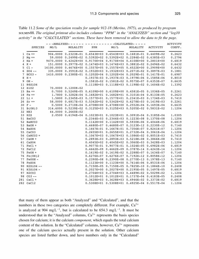
11.3 Components and species 325
Table 11.2 Some of the speciation results for sample 912-18 (Merino, 1975), as produced by programsolmin88. The original printout also includes columns “PPM” in the “ANALYZED” section and “log10activity” in the “CALCULATED” sections. These have been removed to allow the data to fit the page.
- - -ANALYZED- - - - - - - - - - - - - - - - -CALCULATED- - - - - ACTIVITYSPECIES MG/L MOLALITY PPM MG/L MOLALITY ACTIVITY COEFF.
1 Ca ++ 904.0000 0.2323E-01 0.6543E+03 0.6543E+03 0.1681E-01 0.4409E-02 0.26232 Mg ++ 59.0000 0.2499E-02 0.5392E+02 0.5392E+02 0.2284E-02 0.6385E-03 0.27963 Na + 9470.0000 0.4242E+00 0.9170E+04 0.9170E+04 0.4108E+00 0.2801E+00 0.68194 K + 151.0000 0.3977E-02 0.1474E+03 0.1474E+03 0.3881E-02 0.2496E-02 0.64325 Cl - 16100.0000 0.4676E+00 0.1557E+05 0.1557E+05 0.4522E+00 0.2909E+00 0.64326 SO4 -- 335.0000 0.3591E-02 0.1932E+03 0.1932E+03 0.2071E-02 0.3897E-03 0.18817 HCO3 - 1410.0000 0.2380E-01 0.1202E+04 0.1202E+04 0.2029E-01 0.1417E-01 0.69878 H + 0.1937E-03 0.1937E-03 0.1979E-06 0.1585E-06 0.80109 OH - 0.1581E-02 0.1581E-02 0.9575E-07 0.6353E-07 0.6635
11 H4SiO4 0.1118E+03 0.1118E+03 0.1198E-02 0.1604E-02 1.339212 SiO2 70.0000 0.1200E-0215 Ba ++ 0.7000 0.5249E-05 0.6109E+00 0.6109E+00 0.4581E-05 0.1036E-05 0.226118 Fe ++ 1.7800 0.3282E-04 0.1682E+01 0.1682E+01 0.3101E-04 0.8133E-05 0.262322 Li + 1.5800 0.2345E-03 0.1577E+01 0.1577E+01 0.2341E-03 0.1734E-03 0.741026 Sr ++ 58.0000 0.6817E-03 0.5342E+02 0.5342E+02 0.6278E-03 0.1419E-03 0.226130 F - 0.5000 0.2710E-04 0.4708E+00 0.4708E+00 0.2552E-04 0.1693E-04 0.663531 B(OH)3 314.6000 0.5239E-02 0.3125E+03 0.3125E+03 0.5205E-02 0.5831E-02 1.120432 NH3 44.0000 0.2660E-0233 H2S 2.0500 0.6194E-04 0.1023E+01 0.1023E+01 0.3091E-04 0.3185E-04 1.030551 BaCO3 0.2344E-03 0.2344E-03 0.1223E-08 0.1370E-08 1.120452 BaHCO3 0.1142E+00 0.1142E+00 0.5930E-06 0.4044E-06 0.681953 BaOH + 0.4680E-07 0.4680E-07 0.3123E-12 0.2230E-12 0.714054 BaSO4 0.1667E-01 0.1667E-01 0.7356E-07 0.8241E-07 1.120455 CaCO3 0.2655E+01 0.2655E+01 0.2732E-04 0.3061E-04 1.120456 CaHCO3 + 0.1067E+03 0.1067E+03 0.1086E-02 0.8051E-03 0.741057 CaOH + 0.2893E-03 0.2893E-03 0.5218E-08 0.3866E-08 0.741061 CaSO4 0.4045E+02 0.4045E+02 0.3060E-03 0.3428E-03 1.120471 FeCl + 0.9077E-01 0.9077E-01 0.1024E-05 0.6982E-06 0.681972 FeCl2 0.4662E-09 0.4662E-09 0.3787E-14 0.4243E-14 1.120475 FeOH + 0.1619E-02 0.1619E-02 0.2288E-07 0.1634E-07 0.714076 Fe(OH)2 0.6276E-07 0.6276E-07 0.7192E-12 0.8058E-12 1.120477 FeOOH - 0.2390E-08 0.2390E-08 0.2770E-13 0.1978E-13 0.714078 FeSO4 0.1123E+00 0.1123E+00 0.7614E-06 0.8531E-06 1.120490 H2SiO4 -- 0.7150E-05 0.7150E-05 0.7825E-10 0.1884E-10 0.240891 H3SiO4 - 0.2027E+00 0.2027E+00 0.2195E-05 0.1497E-05 0.681997 H2CO3 0.2704E+03 0.2704E+03 0.4489E-02 0.5029E-02 1.120498 CO3 -- 0.1012E+01 0.1012E+01 0.1737E-04 0.4183E-05 0.2408
281 CaCl + 0.3628E+03 0.3628E+03 0.4946E-02 0.3373E-02 0.6819282 CaCl2 0.5308E+01 0.5308E+01 0.4925E-04 0.5517E-04 1.1204
that many of them appear as both “Analyzed” and “Calculated”, and that thenumbers in these two categories are completely different. For example, Ca2+
is analyzed at 904 mgL−1, but is calculated to be 654.3 mgL−1. It must beunderstood that in the “Analyzed” columns, Ca2+ represents the basis specieschosen for calcium; it is the calcium component, which equals the total calciumcontent of the solution. In the “Calculated” columns, however, Ca2+ representsone of the calcium species actually present in the solution. Other calciumspecies are listed further down, and have numbers only in the “Calculated”
326 The phase rule
columns. The sum of the molalities of all Ca-containing species is equal to theinput value of 0.023 23 molal.
Another example of this important difference is provided by the results forsilica. The analyzed silica content (Table 11.1) is 70 mgL−1, and this appears asthe basis species SiO2. This has been converted by the program into a molalityof 0.0012. In many applications, SiO2�aq� and H4SiO4 are used synonymouslyas the uncharged monomeric aqueous silica species. But here, SiO2 is the totalsilica and the “Calculated” amount of H4SiO4 is 0.001 198, a bit less. This isbecause the basis species SiO2 has been split up by the program into the threesecondary species H4SiO4, H3SiO
−4 , and H2SiO
2−4 , seen further down in the
results. The sum of the molalities of these three species is equal to the inputvalue, 0.0012 molal.
11.4 Duhem’s theorem
11.4.1 Traditional components versus basis species
The Gibbs phase rule deals only with intensive variables. It is the same whetheryou have 1 kg or 100 kg of your system. But if you are interested in howa solution changes composition when halite is precipitated from it, say inmodeling evaporation in a closed basin, you need to know how much solutionthere is and how much halite precipitates. You need an extensive phase rule.This was provided by Pierre Duhem, a contemporary of Gibbs, in the form ofDuhem’s theorem. We will lead into this by looking more closely at our twokinds of components – “traditional” and basis species. Readers familiar withMorel and Hering (1993) will recognize that what we have termed “traditional”components are Morel and Hering’s “recipes”, and what we refer to as basisspecies they call simply components.
For the system NaCl–H2O, we have either the two “traditional” componentsNaCl and H2O, which allow us to describe the bulk composition of all phasesin this system, or we have the four basis species Na+, Cl−, H+, and H2O,which allow us to describe not only the compositions of the phases but also theconcentration of all dissolved species in the system. “Traditional” componentsand basis species are simply different choices of components, which havedifferent purposes and different descriptive powers. We need more basis speciesbecause they are called upon to provide more information.
We discussed the system NaCl–H2O in §11.2.1 in terms of the traditionalcomponents, NaCl and H2O. If, however, we use basis species as compo-nents, we will have more degrees of freedom to deal with. For example, usingcomponents NaCl and H2O, we have no control over the Na/Cl ratio, but usingbasis species Na+, Cl−, H+, and H2O, we do – we can specify Na+ and Cl−
independently – an extra degree of freedom. The principles involved have notchanged, so we can use a modified phase rule, but in dealing with aqueous
11.4 Duhem’s theorem 327
solutions we invariably are at a fixed T and P, so we can start with the min-eralogical phase rule (11.3). So instead of f = c−p, with c the number oftraditional components, it becomes
f = b−p (11.4)
where b is the number of basis species needed to define the system; and in thiscase b = 4.
Fortunately, this is fairly intuitive. It just says that to define an aqueoussolution (p = 1) at a given T and P, we have to specify the concentration ofeach solute element. That is, since H2O is always one of the basis species,then there are (b− 1) degrees of freedom, which is evidently the number ofsolute basis species (Na+, Cl−, and H+). Each additional phase present fixesthe value of one basis species, and hence reduces by one the number of basisspecies that must be specified.2
Charge balanceThese basis species are actually not completely independent of one another,as theoretically required, because the sum of the positive and negative chargesmust be equal – there must be a charge balance in real solutions. However, thecharge balance requirement does not really reduce the degrees of freedom. Itjust means that one of the charged basis species, say Cl−, should be adjustedto give the balance. The charge balance requirement is thus substituted for therequirement that basis species Cl− be specified.
11.4.2 The extensive phase rule
Each of the phase rules above is used to “define the equilibrium state,” whichmeans that they each relate the number of properties (understood to be intensivevariables) of the system to the number of degrees of freedom. This “defines”the equilibrium state, but it does not define how much of the equilibrium statewe have. The “equilibrium state” of 1 kg of water saturated with halite is thesame whether we have 1 g or 1 kg of halite. But modeling programs commonlywant to do more than to define the equilibrium state. They want to dissolveor precipitate phases during processes controlled by the modeler, and to keeptrack of the masses involved, so as to know when phases should appear ordisappear. To do this, the mass of each phase is required, not just its presenceor absence. Therefore, an additional piece of information is required for eachphase present, or p quantities. Almost invariably, the mass of H2O is chosen
2 For example, if halite was present at equilibrium, we would specify either the Na+ or the Cl−
basis species, but not both. The other would be fixed through the solubility product. Thus anadditional phase always reduces the number of independent basis species by one.
328 The phase rule
as 1 kg, so that the concentration of basis species defines the mass of each.3
If solid or gas phases are specified, the mass is usually also specified. If wecount these extra p pieces of data, the extensive phase rule becomes
f = b (11.5)
This assumes T and P have been chosen, so they are not included as degreesof freedom. To include these degrees of freedom, we would write (11.5) as
f = b+2 (11.6)
This relationship is also fairly intuitive. Look at it this way. The number ofphases is always at least one (a system with no phases is not very interesting).To define a system having only an aqueous solution phase (p = 1), we mustspecify each of the solutes in the water, or b− 1 quantities. If there is onemineral in equilibrium with the water (p= 2), it controls one basis species, andso reduces b by one, and similarly for all p mineral or gas phases. This is phaserule (11.4). But defining the equilibrium state is not usually enough. We wantalso to know the mass of each phase, so we need p extra data, giving phaserule (11.5), which says that for any system we need b pieces of information.These b pieces of information are
• the mass of water (almost always 1 kg);• the mass of each mineral or gas phase;• the concentration of basis species beyond those controlled by the mineral and gas
phases.
An example will help to clarify this (see the box on page 329). However,if you find this confusing, you are not alone, and perhaps it is not terriblyimportant. The traditional Gibbs phase rule is often used in a “paper andpencil” sense by petrologists interpreting some sequence of rocks, but whendealing with electrolyte solutions and basis species, well-established computerprograms are generally used (Chapter 18). So although the extensive phase ruledoes tell you how many pieces of data are required as input to the program,most people do not figure this out before using the program.
If you were starting from scratch, with no program, this information wouldundoubtedly be useful, but when using well-established programs, it is oftenmore efficient to bypass the phase rule, and rely on error messages from themodeling program to get things right. It is useful, though, to know that thephase rule used or implied in modeling aqueous solutions is somewhat differentfrom the one derived by Gibbs.
3 The unit of concentration used in modeling calculations is invariably molality, or the moles ofsolute species per kilogram of pure water. Therefore, if the mass of water is fixed at 1 kg, themolality of a species automatically equals the number of moles of the species, which is readilyconvertible to grams.
11.4 Duhem’s theorem 329
Example Phase rules
Consider a system consisting of water and dissolved Al, Si and K. If these solutes
are sufficiently concentrated, aluminosilicate minerals will precipitate. Let’s say
that our T and P have been specified as 25 �C and 1 bar.
• “Traditional” components for this system would be K2O, Al2O3, SiO2, and
H2O, so c = 4. If the solutes are very dilute and we have only one phase
(water), phase rule (11.3) says f = c− 1 = 3, so we have to specify the
concentrations of K, Al and Si to define the system. But if we have three
solid phases in equilibrium with the water, such as kaolinite, muscovite, and
quartz, then f = c−p = 0, and the system is invariant (we don’t have to
specify anything). However, even though all properties of the system are
fixed, including the species in the liquid phase, we are unable to describe or
calculate the ionic species using these components.• Alternatively, we choose as the basis the five basis species (or component
species) H2O, K+, Al3+, H+, and SiO2�aq�, thus b = 5. With only water
present, phase rule (11.4) says that we need to specify f = 5− 1 = 4 con-
centrations, which could be the total amounts of K, Al, Si, plus the pH.
With kaolinite, muscovite and quartz present in any amount at equilibrium,
phase rule (11.4) says that f = 5− 4 = 1, so we need to specify only one
concentration to be invariant. In either case, i.e., whether we have specified
one or four concentration(s), we are able to describe and calculate all ionic
species present.• Extensive phase rule (11.5) then says that even though we are invariant,
that is, even though we have adequately described the equilibrium state, to
make our description more useful we need f = b = 5 pieces of information:
either (with only water) the four concentrations and the mass of water, or
(with water and three minerals) one concentration plus the masses of all four
phases.
What Duhem saidThe term “extensive phase rule” is more commonly referred to as Duhem’stheorem. As expressed by Prigogine and Defay (1965), p. 188, Duhem’stheorem says
Whatever the number of phases, of components or of chemical reactions, the
equilibrium state of a closed system, for which we know the initial masses
m�1 m
�c , is completely determined by two independent variables.
The big difference from the Gibbs phase rule is of course the inclusion of “theinitial masses m�
1 m�c,” so that in addition to T and P we need to know
330 The phase rule
the mass of every traditional component, if we are not concerned with ionicspeciation, or every basis species, if we are (Equation 11.6).
The phase rule is a very beautiful example of the interface between mathe-matics and physical reality.
11.5 Buffered systems
A great deal of the power and usefulness of the phase rule in geochemistrycomes from its demonstration of which systems are divariant, and which there-fore have all their properties fixed at a given T and P. Changing the concen-tration of any component of a trivariant or multivariant solution will changeall the properties of the solution, even if T and P do not change. However,consider a divariant system at fixed values of T and P.
11.5.1 Divariant systems
Divariant systems are of course those that have the same number of componentsand phases. Because the presence of a certain number of phases fixes all theproperties of the system at given T and P, including the compositions of allphases, the system has a certain resistance to any process attempting to changethese properties, and it will continue to resist change until the process inquestion succeeds in decreasing the number of phases. The system is thereforesaid to be “buffered.” For example, a rock consisting of gypsum �CaSO4 ·2H2O�and anhydrite �CaSO4� has two phases and two components, so its propertiesare fixed at a given T and P. Thus the activity of water is fixed through therelation
12CaSO4 ·2H2O= 1
2CaSO4+H2O
for which
K = a0�5CaSO4aH2O
a0�5CaSO4 ·2H2O
= aH2Owhen aCaSO4 ·2H2O
= aCaSO4= 1
If the standard states for the solid phases are the pure phases at T and P, theiractivities are both one, and the equilibrium constant equals the activity of water,i.e., the activity of water is a constant (fixed) as long as (pure) gypsum andanhydrite coexist. Water having some other greater activity introduced alongcracks in this rock will tend to change the activity of water in the system, butno change will in fact take place (at least in the model) until all the anhydriteis converted to gypsum, at which point the system is no longer buffered andthe water activity can assume a new value fixed by the introduced water.
11.5 Buffered systems 331
Systems having fewer than two degrees of freedom (that is, one or zero) arealso of course buffered in the same way. A pure component at its melting pointfor example (c = 1, p = 2, f = 1) is buffered against changes in temperatureor pressure. If heat is added, the temperature does not rise until the solid phasehas disappeared. Divariant systems at a given T and P are also in principlebuffered against changes in T and P, but unless reactions with a large �H or�V are involved, which generally means a melting or vaporization reaction,the buffering effect will be small. Thus the principle of buffering shouldnot be confused with the buffering capacity, which depends on the reactionsinvolved and the amounts and proportions of the phases. Univariant systemsare particularly important in metamorphic petrology where they are known asisograds. Invariant systems are quite rare in nature but at least one is fairlycommon in the laboratory; the ice–water–water vapor triple point is frequentlyused in the calibration of thermometers at 273.16 K.
11.5.2 Buffered experimental systems
This property (of resisting change) of systems having two (or fewer) degrees offreedom has been known for over 100 years, so one could be forgiven for beingsurprised at the great change (it’s probably exaggerating to call it a revolution)in geochemical thought and practice brought about when Hans Eugster drewattention to its usefulness in experimental and theoretical work. The originalapplication was a demonstration that the assemblages hematite/magnetite/water,quartz/fayalite/magnetite/water, nickel/nickel oxide/water and others could beused in experimental work to control the oxidation state of experimental systemsby separating the “buffering system” (one of the above) from the experimentalsystem by a membrane (platinum) permeable to hydrogen. The buffer system,having the same number of components as phases, as well as having an element(e.g., Fe, Ni) in two different valence states, fixed the properties of each ofits phases, and in particular fixed the oxygen and hydrogen fugacities in thewater. Typical buffering reactions are
H2O+2Fe3O4 (Magnetite)= 3Fe2O3 (Hematite)+H2�g�
Ni�s�+H2O= NiO (Bunsenite)+H2�g�
The hydrogen diffused through the capsule walls and controlled the oxidationstate of the experimental system, which also included an aqueous phase. Thisarrangement is illustrated in Figure 11.1.
The buffer system thus “imposes” its oxidation state on the experimentalsystem, and will continue to do so for some time even if the experimentalsystem consumes hydrogen or oxygen in its reactions. Since then, innumerablebuffering systems and experimental arrangements have been devised, the detailsof which, being all based on the same principle, are not of great interest
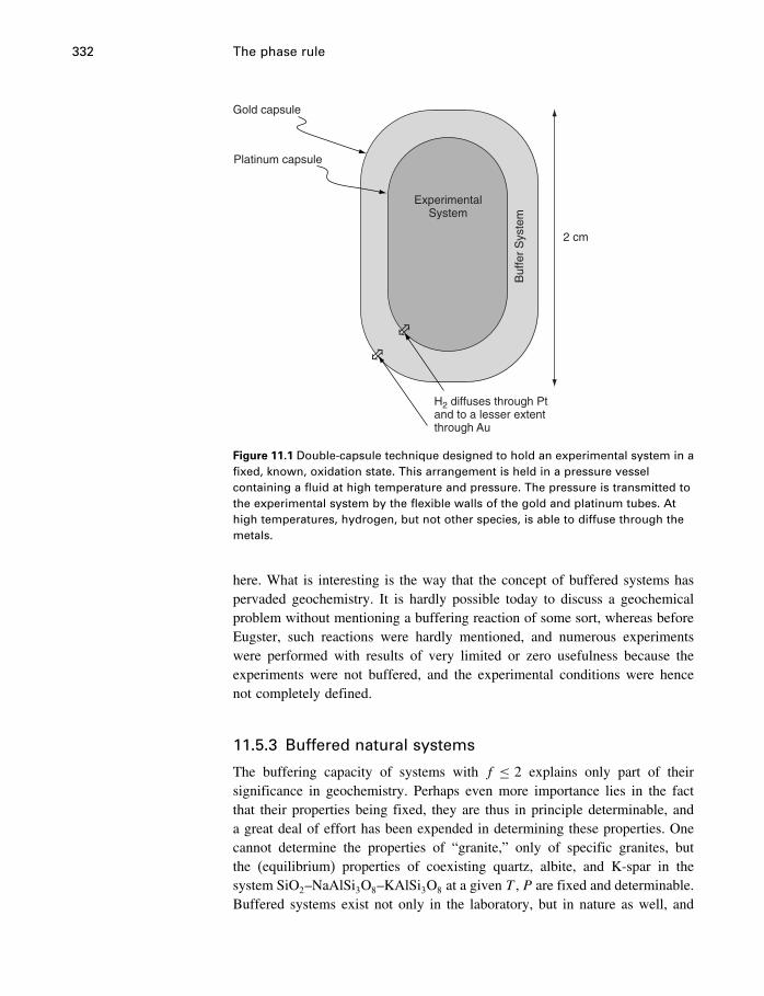
332 The phase rule
2 cm
Gold capsule
Platinum capsule
ExperimentalSystem
Buf
fer
Sys
tem
H2 diffuses through Ptand to a lesser extentthrough Au
⇔
⇔
Figure 11.1 Double-capsule technique designed to hold an experimental system in afixed, known, oxidation state. This arrangement is held in a pressure vesselcontaining a fluid at high temperature and pressure. The pressure is transmitted tothe experimental system by the flexible walls of the gold and platinum tubes. Athigh temperatures, hydrogen, but not other species, is able to diffuse through themetals.
here. What is interesting is the way that the concept of buffered systems haspervaded geochemistry. It is hardly possible today to discuss a geochemicalproblem without mentioning a buffering reaction of some sort, whereas beforeEugster, such reactions were hardly mentioned, and numerous experimentswere performed with results of very limited or zero usefulness because theexperiments were not buffered, and the experimental conditions were hencenot completely defined.
11.5.3 Buffered natural systems
The buffering capacity of systems with f ≤ 2 explains only part of theirsignificance in geochemistry. Perhaps even more importance lies in the factthat their properties being fixed, they are thus in principle determinable, anda great deal of effort has been expended in determining these properties. Onecannot determine the properties of “granite,” only of specific granites, butthe (equilibrium) properties of coexisting quartz, albite, and K-spar in thesystem SiO2–NaAlSi3O8–KAlSi3O8 at a given T , P are fixed and determinable.Buffered systems exist not only in the laboratory, but in nature as well, and
11.5 Buffered systems 333
other natural systems can be seen to have properties intermediate betweenthose of certain buffered systems, so that the buffering concept provides aframework for thinking about natural systems. For example, hematite andmagnetite coexist in many iron formations, and rocks containing magnetite butnot hematite or wüstite (FeO) are thought of as lying between the magnetite–hematite and magnetite–wüstite buffers in terms of oxidation state. Similarlysyenites containing no quartz and no nepheline can be thought of as lyingbetween the quartz and albite–nepheline buffers for SiO2.
In view of the fact that the majority of experimental applications of thebuffering principle have been in the control of specific gaseous or aqueousspecies, we should perhaps reiterate that in a buffered system all properties arefixed, and that completely solid systems are no exception. Thus for examplealthough the assemblage hematite–magnetite buffers the activity of oxygenthrough the reaction
6Fe2O3 = 4Fe3O4+O2
it also buffers the FeO activity through
Fe3O4 = Fe2O3+FeO
the Fe activity through
3Fe3O4 = 4Fe2O3+Fe
the O3 activity through
9Fe2O3 = 6Fe3O4+O3
as well as the activity of any other conceivable components of the Fe–O system.
11.5.4 Absolute versus relative buffers
The system having at least as many phases as components can be thought of asa kind of “absolute” buffer. That is, the properties of all phases are absolutelydetermined once the remaining variables are chosen, and of course once equi-librium is achieved. The system properties, dozens of them, are state variables,are independent of the system’s history, and in principle are determinable,given enough data. We add to this statement once more the cautionary notethat in nature a buffering assemblage may not in fact have buffered anything,because of being present in too small a quantity, i.e., the buffering capacity mayhave been negligible, or because of unfavorable kinetics. Such assemblages arenevertheless always of interest in interpretations of geological history, becausethey are locations where thermodynamic parameters have a fixed and oftenknown relationship.
334 The phase rule
Many systems having f ≥ 3 are also spoken of as buffers. The most commonexamples are of course the aqueous buffers so commonly used in chemistry,usually to control the pH of a solution. For example, a solution containingsodium acetate and acetic acid will resist changes in pH when an acid orbase is added due to the common ion effect. The pH does not change asmuch as it would if the NaAc and HAc were not there, but it does change,because the system is not an “absolute” buffer in the sense we have been using.Nevertheless, it does resist change and so is buffered. Other systems can bebuffered simply due to the large mass involved. Thus the chlorine concentrationof the ocean is not controlled by any process or reaction, but pouring salt intothe ocean doesn’t change it at all; it is buffered by the sheer size of the system.
11.6 Summary
The phase rule is a relationship between the number of components, phasesand degrees of freedom in a system at equilibrium. It has an exact analogywith a system of linear equations, because it is derived from such a system.The original phase rule derived by Gibbs (typically, in a few lines, no bigdeal) applies to intensive variables only; it is independent of the mass ofthe system. Later, Duhem’s theorem extended the phase rule to extensivevariables. It is this version which is implicit in most modeling of geochemicalprocesses, because such models must take into account the appearance anddisappearance of phases. Understanding either version of the phase rule requiresunderstanding the various usages of the terms “component” and “species.”One of the most fruitful deductions from the phase rule is the principle of“absolute” buffering, which has been widely applied in experimental work andin theoretical discussions.
The phase rule is one of the most impressive and, yes, beautiful, resultsin all of equilibrium thermodynamics. It has proven essential in the study ofexperimental and natural systems.
12Redox reactions
12.1 Introduction
Normal seawater contains about 2660 ppm (0.028m) of sulfur in the form ofsulfate (SO2−
4 ). Sulfur in this form has a valence of +6, meaning that it has sixfewer electrons per atom than has native sulfur, which exists (though not in theocean) as a yellow crystalline solid. In some parts of the ocean, however, sulfurexists in the form of dissolved hydrogen sulfide, H2S�aq�. Sulfur in this formhas a valence of −2, meaning that it has two extra electrons compared to nativesulfur, and in this form it is a deadly poison. Those parts of the ocean containingthis electron-rich form of sulfur contain no living organisms other than a fewkinds of bacteria. Obviously, the number of electrons that each sulfur atom hasis not a question of interest only to atomic physicists. Changing sulfate-sulfurto H2S-sulfur or vice versa involves transferring electrons from one to the other,and this electron transfer is the basic element of redox (reduction–oxidation)reactions.
Many naturally occurring elements in addition to sulfur show similar vari-ations in their number of electrons, with similar large differences in theirchemical properties. It would be difficult to overemphasize the importance tous of these variations in valence, or numbers of electrons per atom. Biochem-istry, for example, is in large part a study of redox reactions. Because naturalenvironments show great variability in their redox state, we need to developsome kind of measurement, an index, which will be useful in characterizingthese redox states, much as we use pH as a measurement or index to character-ize the acidity of various states, or temperature as a measurement or an indexof the hotness of states. In this chapter we develop two such indexes of redoxstate.
12.2 Electron transfer reactions
You may not have noticed it, but we have considered two kinds of reactionsin previous chapters. In some, such as (9.3),
SiO2�s�+2H2O= H4SiO4�aq�
335
336 Redox reactions
all elements on the right side have the same number of electrons that they haveon the left side – there is no change in valence of any element. In others, suchas (9.16),
CH4�g�+O2�g�= CO2�g�+2H2�g�
there is such a change. For example, the carbon in CH4 is C4−, and the carbon
in CO2 is C4+. Each carbon atom in methane that changes to a carbon atom in
carbon dioxide must get rid of eight electrons – it is oxidized. Where do theelectrons go? Obviously, they go to the other actors in the reaction. Oxygenin O2 has a valence of zero (O0), while in carbon dioxide it is −2 (O2−), soin changing from O2 to CO2, two oxygens gain four electrons. The other fourelectrons go to hydrogen, which has a valence of +1 (H+) in methane and zeroin hydrogen gas. Both oxygen and hydrogen are reduced, if the reaction goesfrom left to right as written. Similarly in reaction (9.15),
6Fe2O3�s�= 4Fe3O4�s�+O2�g�
we see that all of the iron atoms in Fe2O3 are ferric iron (Fe3+), while oneout of three iron atoms in Fe3O4 is ferrous iron (Fe2+). The iron is partiallyreduced, while some oxygen in Fe2O3 is oxidized to O2�g� – there is a transferof electrons from iron to oxygen, or from oxygen to iron, depending on whichway the reaction goes. Without such electron transfers, these and many otherreactions, including many necessary to life processes, could not proceed.
12.3 The role of oxygen
Both of our examples involve oxygen, which is the most common oxidizingagent in natural systems. In the presence of oxygen, many elements are oxidized(lose electrons, gain in valence), while oxygen is reduced. You need only thinkof rusty nails, green staining on copper objects, and burning logs to realize thetruth of this. The process of oxidation obviously takes its name from the factthat oxygen is the premier oxidizing agent, but it is actually defined in termsof electron loss, or increase in valence. In other words, the electrons need notcome from or go to oxygen; many redox reactions take place without oxygen.
Consider, for example, what happens when you put a piece of iron in asolution of copper sulfate (Figure 12.1). After a while you see the characteristiccolor of metallic copper forming on the surface of the iron, and the irongradually crumbles and eventually disappears. Metallic copper precipitates, andiron dissolves. The reaction is essentially
Cu2++Fe→ Cu+Fe2+ (12.1)
We need not include the sulfate, because it is not involved in this process –being negatively charged, the SO2−
4 ions provide an overall charge balance in
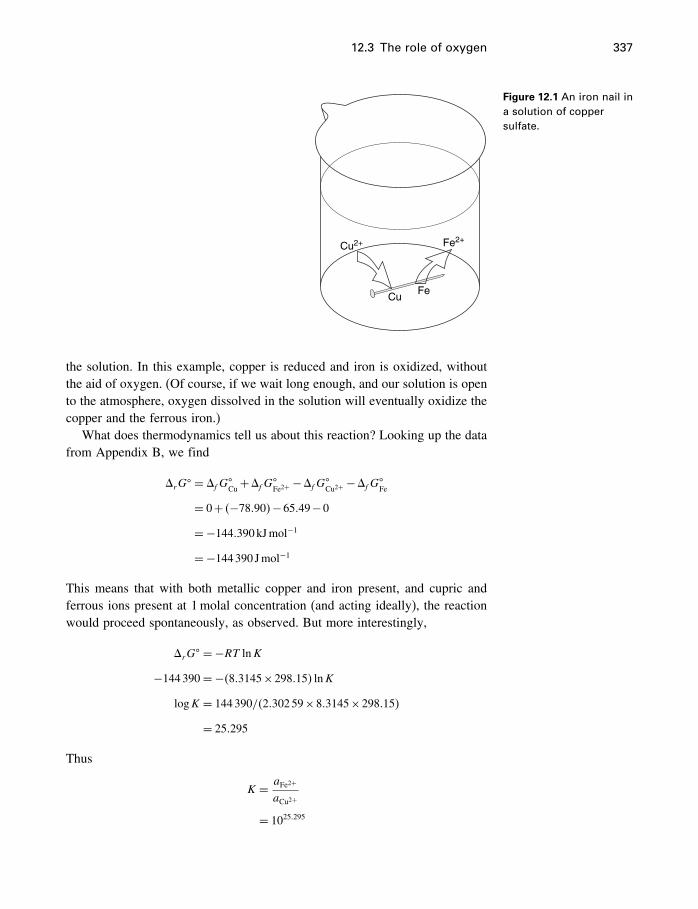
12.3 The role of oxygen 337
FeCu
Cu2+ Fe2+
Figure 12.1 An iron nail ina solution of coppersulfate.
the solution. In this example, copper is reduced and iron is oxidized, withoutthe aid of oxygen. (Of course, if we wait long enough, and our solution is opento the atmosphere, oxygen dissolved in the solution will eventually oxidize thecopper and the ferrous iron.)
What does thermodynamics tell us about this reaction? Looking up the datafrom Appendix B, we find
�rG� = �fG
�Cu+�fG
�Fe2+ −�fG
�Cu2+ −�fG
�Fe
= 0+ �−78�90�−65�49−0
=−144�390kJmol−1
=−144390 Jmol−1
This means that with both metallic copper and iron present, and cupric andferrous ions present at 1molal concentration (and acting ideally), the reactionwould proceed spontaneously, as observed. But more interestingly,
�rG� = −RT lnK
−144390=−�8�3145×298�15� lnK
logK = 144390/�2�30259×8�3145×298�15�
= 25�295
Thus
K = aFe2+
aCu2+
= 1025�295
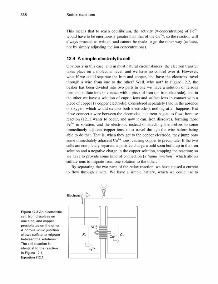
338 Redox reactions
This means that to reach equilibrium, the activity (≈concentration) of Fe2+
would have to be enormously greater than that of the Cu2+, so the reaction willalways proceed as written, and cannot be made to go the other way (at least,not by simply adjusting the ion concentrations).
12.4 A simple electrolytic cell
Obviously in this case, and in most natural circumstances, the electron transfertakes place on a molecular level, and we have no control over it. However,what if we could separate the iron and copper, and have the electrons travelthrough a wire from one to the other? Well, why not? In Figure 12.2, thebeaker has been divided into two parts.In one we have a solution of ferrousions and sulfate ions in contact with a piece of iron (an iron electrode), and inthe other we have a solution of cupric ions and sulfate ions in contact with apiece of copper (a copper electrode). Considered separately (and in the absenceof oxygen, which would oxidize both electrodes), nothing at all happens. Butif we connect a wire between the electrodes, a current begins to flow, becausereaction (12.1) wants to occur, and now it can. Iron dissolves, forming moreFe2+ in solution, and the electrons, instead of attaching themselves to someimmediately adjacent copper ions, must travel through the wire before beingable to do that. That is, when they get to the copper electrode, they jump ontosome immediately adjacent Cu2+ ions, causing copper to precipitate. If the twocells are completely separate, a positive charge would soon build up in the ironsolution and a negative charge in the copper solution, stopping the reaction; sowe have to provide some kind of connection (a liquid junction), which allowssulfate ions to migrate from one solution to the other.
By separating the two parts of the redox reaction, we have caused a currentto flow through a wire. We have a simple battery, which we could use to
Figure 12.2 An electrolyticcell. Iron dissolves onone side, and copperprecipitates on the other.A porous liquid junctionallows sulfate to migratebetween the solutions.The cell reaction isidentical to the reactionin Figure 12.1,Equation (12.1).
Electrons
Fe CuCu2+
Fe2+
SO2–4
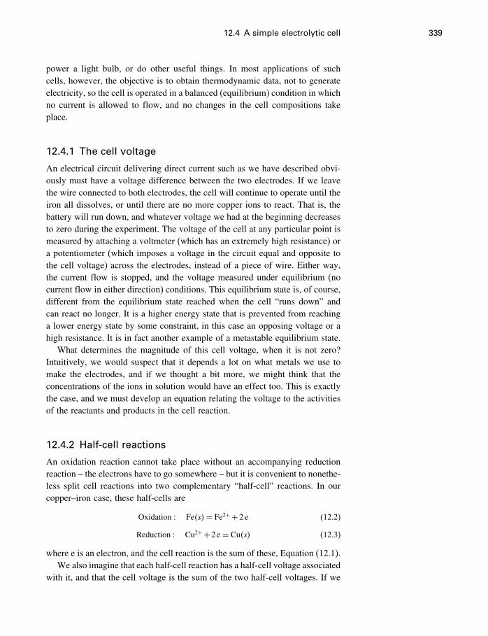
12.4 A simple electrolytic cell 339
power a light bulb, or do other useful things. In most applications of suchcells, however, the objective is to obtain thermodynamic data, not to generateelectricity, so the cell is operated in a balanced (equilibrium) condition in whichno current is allowed to flow, and no changes in the cell compositions takeplace.
12.4.1 The cell voltage
An electrical circuit delivering direct current such as we have described obvi-ously must have a voltage difference between the two electrodes. If we leavethe wire connected to both electrodes, the cell will continue to operate until theiron all dissolves, or until there are no more copper ions to react. That is, thebattery will run down, and whatever voltage we had at the beginning decreasesto zero during the experiment. The voltage of the cell at any particular point ismeasured by attaching a voltmeter (which has an extremely high resistance) ora potentiometer (which imposes a voltage in the circuit equal and opposite tothe cell voltage) across the electrodes, instead of a piece of wire. Either way,the current flow is stopped, and the voltage measured under equilibrium (nocurrent flow in either direction) conditions. This equilibrium state is, of course,different from the equilibrium state reached when the cell “runs down” andcan react no longer. It is a higher energy state that is prevented from reachinga lower energy state by some constraint, in this case an opposing voltage or ahigh resistance. It is in fact another example of a metastable equilibrium state.
What determines the magnitude of this cell voltage, when it is not zero?Intuitively, we would suspect that it depends a lot on what metals we use tomake the electrodes, and if we thought a bit more, we might think that theconcentrations of the ions in solution would have an effect too. This is exactlythe case, and we must develop an equation relating the voltage to the activitiesof the reactants and products in the cell reaction.
12.4.2 Half-cell reactions
An oxidation reaction cannot take place without an accompanying reductionreaction – the electrons have to go somewhere – but it is convenient to nonethe-less split cell reactions into two complementary “half-cell” reactions. In ourcopper–iron case, these half-cells are
Oxidation � Fe�s�= Fe2++2 e (12.2)
Reduction � Cu2++2 e= Cu�s� (12.3)
where e is an electron, and the cell reaction is the sum of these, Equation (12.1).We also imagine that each half-cell reaction has a half-cell voltage associated
with it, and that the cell voltage is the sum of the two half-cell voltages. If we
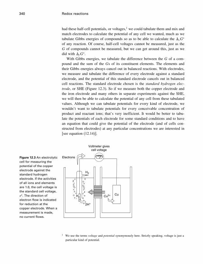
340 Redox reactions
had these half-cell potentials, or voltages,1 we could tabulate them and mix andmatch electrodes to calculate the potential of any cell we wanted, much as wetabulate Gibbs energies of compounds so as to be able to calculate the �rG
�
of any reaction. Of course, half-cell voltages cannot be measured, just as theG of compounds cannot be measured, but we can get around this, just as wedid with �fG
�.With Gibbs energies, we tabulate the difference between the G of a com-
pound and the sum of the Gs of its constituent elements. The elements andtheir Gibbs energies always cancel out in balanced reactions. With electrodes,we measure and tabulate the difference of every electrode against a standardelectrode, and the potential of this standard electrode cancels out in balancedcell reactions. The standard electrode chosen is the standard hydrogen elec-trode, or SHE (Figure 12.3). So if we measure both the copper electrode andthe iron electrode and many others in separate experiments against the SHE,we will then be able to calculate the potential of any cell from these tabulatedvalues. Although we can tabulate potentials for every kind of electrode, wewouldn’t want to tabulate potentials for every conceivable concentration ofproduct and reactant ions; that’s very inefficient. It would be better to tabu-late the potentials of each electrode for some standard conditions and to havean equation that could give the potential of the electrode (and of cells con-structed from electrodes) at any particular concentrations we are interested in[see equation (12.14)].
Figure 12.3 An electrolyticcell for measuring thepotential of the copperelectrode against thestandard hydrogenelectrode. If the activitiesof all ions and elementsare 1.0, the cell voltage isthe standard cell voltage,��. The direction ofelectron flow is indicatedfor reduction at thecopper electrode. When ameasurement is made,no current flows.
Voltmeter givescell voltage
Electrons
H2
H2
2H+
Cu2+ Cu
–
1 We use the terms voltage and potential synonymously here. Strictly speaking, voltage is just aparticular kind of potential.
12.5 The Nernst equation 341
12.4.3 Standard electrode potentials
A cell for measuring the potential of the copper–SHE cell is shown inFigure 12.3.The hydrogen electrode is a device for using the reaction
2H++2 e� H2�g� (12.4)
as an electrode.The idea of using a gas as an electrode seems rather bizarre atfirst. It is accomplished by bubbling hydrogen gas over a specially treated pieceof platinum (platinum coated with fine-grained carbon). The platinum servessimply as a source or sink of electrons; the reaction between hydrogen gas andhydrogen ions takes place at the surface of the platinum and is catalyzed bythe carbon.
In order that the hydrogen electrode always give the same potential, theactivities of both the hydrogen gas and the hydrogen ion must always be thesame. These have been standardized at fH2�g�
= 1bar, and aH+ = 1, that is, a gaspressure of one bar, and an acid concentration of about 1molal. A hydrogenelectrode operating under these conditions, the standard hydrogen electrode, isassigned a half-cell potential of zero volts by convention.
The half-cell reactions for the cell in Figure 12.3 are
Oxidation � H2�g�= 2H++2 e (12.5)
Reduction � Cu2++2 e= Cu�s� (12.6)
and the sum of these is the cell reaction
Cu2++H2�g�= Cu�s�+2H+ (12.7)
As we mentioned, the cell voltage depends on the activities of all the ions andcompounds in the cell reaction; in this case it depends not only on the hydrogengas pressure and aH+ , but on aCu and aCu2+ as well. “Standard conditions” isdefined as a = 1 for all products and reactants in the cell reaction, and so ifthe hydrogen electrode is operating under SHE conditions (aH2�g�
= 1� fH2�g�=
1bar), the copper electrode is pure Cu (aCu�s� = 1) and the cupric ion concen-tration and activity coefficient are adjusted to give aCu2+ = 1, the cell voltagewill be the standard cell voltage, ��.
12.5 The Nernst equation
12.5.1 Work done by cells
In lighting the light bulb or running a small motor, our cell in Figure 12.2is doing work. We have already seen, in Chapter 4, how much work can bedone by a chemical reaction, but you may have forgotten this because we haveput so much emphasis on reactions that do no work, other than the minimumnecessary P�V work. But here we have a chemical reaction that is certainly
342 Redox reactions
doing P�V work (the Fe2+ and Cu in the cell reaction will have a slightlydifferent molar volume than the Fe and Cu2+, and so some work is done againstthe atmospheric pressure on the solution), but in addition to this, it is doingwork in lighting the bulb. According to §4.10, the maximum amount of workwe can get from our cell reaction is given by the �rG of that reaction, andwhen �rG decreases to zero, we reach stable equilibrium and can get no morework from the cell.
The electrical work w required to move a charge of � coulombs through apotential difference � volts is
−w = � �
(joules= coulombs × volts)
where � is the charge per mole of electrons, so if n is the number of electronsappearing in the reaction as written, there are n� coulombs of charge, and thework is
−w = n� � (12.8)
Because some convention must be adopted to know whether the voltage � ispositive or negative, you may see Equation (12.8) [as well as (12.9) and (12.10),below] written without the minus sign in some references. The conventions wehave adopted (§12.6.1) require the minus sign.
This electrical work is by definition (Chapter 4) the �G associated withthe process, as long as the electrical work is the only non-P�V work done.Therefore for any process in which n� coulombs are moved through a potentialdifference ��
�G=−n� � (12.9)
or
�G� = −n� �� (12.10)
for standard state conditions. As applied to electrochemical cells, these equa-tions are more properly �� = −n� � and ��� = −n� �� because many ofthe individual free energy terms refer to constituents in solution and hence arepartial molar terms. These equations connect electrochemistry to the world ofthermodynamics. They allow us to calculate the voltage that will be observedin any cell for which we know the cell reaction and the �rG or the �rG
�.
12.5.2 Relation between cell activities and voltage
Consider the general cell reaction
bB+ cC= dD+ eE (12.11)
12.5 The Nernst equation 343
Let’s say that this reaction reaches equilibrium with an external measuringsystem, giving cell voltage �. If operated under standard conditions, it wouldgive cell voltage ��, and the corresponding Gibbs energies of reaction are
�r�=−n� � (12.12)
and
�r�� = −n� �� (12.13)
From Equation (9.8) we have
�r�= �r�� +RT lnQ [9.8]
where
Q=∏i
a�ii
= aeEadD
abBacC
Recall from Chapter 9 that this activity term is referred to as Q rather than Kbecause it refers to a metastable equilibrium. Substitution of Equations (12.12)and (12.13) gives
� = �� − RT
n�lnQ
or
� = �� −2�30259RT
n�logQ (12.14)
This is the Nernst equation, after the physical chemist W. Nernst, whoderived it at the end of the nineteenth century. As above, n is the number ofelectrons transferred in the cell reaction (2 in reaction 12.7), � the Faraday ofcharge, R the gas constant, and T the temperature (in kelvins). The constant2.302 59 is used to convert from natural to base 10 logs. At 25 �C the quantity2�30259 RT/� has the value 0.059 16, which is called the Nernst slope. Theimportance of (12.14) is that it allows calculation of the potentials of cellshaving nonstandard state concentrations (i.e., real cells) from tabulated valuesof standard half-cell values or tabulated standard Gibbs energies.
Equation (12.11) could also be considered to represent a half-cell reaction,except that the electron is not shown. So evidently we could use the Nernstequation to calculate half-cell potentials if we knew what value to assign thechemical potential of an electron. It turns out, of course, that because theelectrons always cancel out in balanced reactions, we could assign any valuewe like to the electron Gibbs energy and it would make no difference to ourcalculated cell potentials. The easiest value to assign is zero, and that is whatis done. Therefore, the Nernst equation is used to calculate both half-cell andcell potentials.
344 Redox reactions
12.6 Some necessary conventions
In our discussion so far, we have skipped lightly over some points which arenot important to a general understanding, but which if neglected will result ingetting the wrong answers in calculations. For example, we said (§12.4.2) thatthe cell voltage is the sum of the two half-cell voltages. Actually, it is a littlemore complicated. Because half-cell and cell reactions may be written forwardsor backwards, and a voltage by itself is not obviously positive or negative,there has to be a set of rules to keep things straight. Unfortunately, there ismore than one set of rules. We present here the rules set out by the IUPAC(International Union of Pure and Applied Chemistry), which are followed bymost people today. Be warned, however, that several geochemical sources usea different set of rules.
12.6.1 The IUPAC rules
Some of these points have been already discussed. We include all the ruleshere for completeness.
1. Cell reactions are written such that the left-hand electrode supplies electrons to
the outer circuit (i.e., oxidation takes place), and the right-hand electrode accepts
electrons from the outer circuit (i.e., reduction takes place).
2. The cell potential is given by
� = �right electrode−�left electrode
that is,
� = �reduction electrode−�oxidation electrode
3. The cell potential is related to the Gibbs energy by
�rG=−n� �
4. The electrode potential of a half-cell is equal in magnitude and sign to the potential
of a cell formed with the electrode on the right and the standard hydrogen electrode
(�� = 0) on the left.
5. Standard half-cell reactions are tabulated and calculated as reductions, for example,
Zn2++2 e= Zn�s� �� = −0�763V
However, the half-cell potential is a sign-invariant quantity, that is,
Zn�s�= Zn2++2 e �� = −0�763V
12.6 Some necessary conventions 345
6. For the reaction
bB+ cC= dD+ eE
the Nernst expression is
� = �� − RT
n�ln(aeEa
dD
abBacC
)
7. In view of item 5, the Nernst expression for a half-cell is given by
� = �� − RT
n�ln(reduced formoxidized form
)
12.6.2 Examples
Let’s calculate the potential of the cell in Figure 12.2. By convention 5, bothhalf-cells are written and calculated as reductions, no matter what is happeningin the real cell. Thus, for the copper half-cell,
Cu2++2 e= Cu�s�
�rG� = �fG
�Cu�s�
−�fG�Cu2+
= 0−65�49kJmol−1
=−65490 Jmol−1
=−n� ��
Because two electrons are involved, n= 2, so
��Cu half-cell =− −65490
2×96485
= 0�339V
For the iron half-cell,
Fe2++2 e= Fe�s�
�rG� = �fG
�Fe�s�
−�fG�Fe2+
= 0− �−78�90�kJmol−1
= 78900 Jmol−1
=−n� ��
��Fe half-cell =− 78900
2×96485
=−0�409V
346 Redox reactions
For the complete cell,
��Cu−Fe cell = ��
reduction half-cell−��oxidation half-cell
= ��Cu half-cell−��
Fe half-cell
= 0�339− �−0�409�
= 0�748V
Note that if we wrote the cell backwards,
Cu�s�+Fe2+ = Cu2++Fe�s�
both half-cell reactions would still be written and calculated as reductions, butthe cell voltage would now be
��Cu−Fe cell = ��
reduction half-cell−��oxidation half-cell
= ��Fe half-cell−��
Cu half-cell
=−0�409− �0�339�=−0�748V
Thus the signs of both �rG� and �� of the complete cell reaction depend on
how the cell is written, but the signs of the half-cell reactions do not.These are the standard potentials. Suppose the cell is operating under
nonstandard (real) conditions. Let’s say aCu2+ is not 1 but 0.1, and aFe2+is 1.5. Using the Nernst expression for the complete cell (reaction 12.1)at 25 �C,
� = �� −2�30259RT
n�logQ
= �� − 0�05916n
logaFe2+
aCu2+
= 0�748− 0�059162
log1�50�1
= 0�748−0�0348
= 0�713V
So the real cell with these concentrations would have a potential of 0.713V,rather than 0.748V.
12.7 Measuring activities 347
The Nernst expression can also be used for the half-cells. Thus for the Cuhalf-cell,
� = �� −2�30259RT
n�logQ
= �� − 0�05916n
logaCuaCu2+
= 0�339− 0�059162
log10�1
= 0�339−0�0296
= 0�309V
and for the Fe half-cell,
� = �� −2�30259RT
n�logQ
= �� − 0�05916n
logaFeaFe2+
= −0�409− 0�059162
log11�5
=−0�409+0�0052
=−0�404V
The cell potential is then
�Cu−Fe cell = �reduction half-cell−�oxidation half-cell
= �Cu half-cell−�Fe half-cell
= 0�309− �−0�404�
= 0�713V
as before.There certainly are other ways to do these calculations and have them come
out right. However, all conventions have their good and bad points, and theIUPAC conventions are the most commonly used.
12.7 Measuring activities
In geochemistry, possibly the greatest interest in galvanic cells is in under-standing the concept of Eh and its use in determining redox conditions innatural environments (§12.8.1). In chemistry, it is in determining the activitiesof solutes.
348 Redox reactions
12.7.1 �� as a source of �fG�
Electrochemical cells are of course of great practical importance in the formof batteries and fuel cells. In thermodynamics, the relationship between cellpotential and Gibbs energy is often used the other way around. That is, cellpotentials are one of the most accurate and useful sources of information aboutGibbs energies of reactions and dissolved substances. Not all Gibbs energydata come from calorimetry. Most data for �fG
�Fe2+ , �fG
�Cu2+ , and other ionic
species come from the measurement of �� in cells such as shown in Figure 12.3.Actually the cells in Figures 12.3 and 12.1 are complicated by a factor we
have not mentioned. These are cells having a junction between two solutionswith different compositions, and this results in an additional source of emf,called a junction potential. It arises because the two solutions must inevitablydiffuse into one another to some extent, however small, and ionic concentrationgradients are established which create a potential difference. This is a majortopic in electrochemistry, but need not be treated in detail here. Suffice it tosay that in the case of Figure 12.3, the liquid junction is not necessary. Thecopper electrode could be placed in the same solution as the hydrogen electrode,as in Figure 12.4, creating a cell without a liquid junction, simplifying thethermodynamic interpretation.
The activity of HClAs an example of the determination of activity of a solute, we consider HCl.A cell much like that in Figure 12.4 but having a standard calomel or silverchloride reference electrode (§12.8.3) in place of the platinum electrode, andhaving a solution of HCl rather than a solution of ferrous and ferric ions, canbe abbreviated as
Pt�H2�g��HCl�aq��AgCl�Ag
where | indicates a phase boundary. With the half-cell reactions
12H2�g�= H++ e
and
AgCl+ e= Ag�s�+Cl−
the cell reaction is
12H2�g�+AgCl= Ag+H++Cl−
or
12H2�g�+AgCl= Ag+HCl
12.8 Measuring redox conditions 349
for which the Nernst equation is
� = �� −2�30259RT
n�logQ [12.14]
= �� −2�30259RT
n�log
aAgaHCl
f1/2H2aAgCl
Because the activity of AgCl and of Ag are fixed at 1.0, the only variables arefH2
and the concentration of HCl, so at a fixed standard state fH2of 1.0 bars,
the cell voltage is a direct measure of the activity of HCl, as long as �� isknown. Determination of �� requires an extrapolation to infinite dilution, andwas the subject of a great deal of research involving the behavior of chargedsolutes in dilute solutions. For our purposes, it is sufficient to see how cellvoltages can be related to solute activities. Some results of these measurementsfor HCl are shown in Figure 15.3.
12.8 Measuring redox conditions
So far we have only considered cells that we might construct ourselves, inthe laboratory. For the scientist interested in natural environments, this isbackground information. What we really want to know is how to characterizenatural environments as being either reducing or oxidizing on some numericalscale. Natural environments don’t normally have electrodes sticking out ofthem, so what is the connection?
In the absence of electrodes and voltages, the redox state of a solution ischaracterized by the relative concentrations of reduced and oxidized ionic ormolecular species in the solution. Thus in a solution containing Fe ions, thesolution is relatively reduced if there are more Fe2+ ions than Fe3+ ions, and viceversa. In a solution containing carbon species, the solution is relatively reducedif there are more CH4 molecules than CO2 molecules. In a solution containingsulfur, the solution is relatively reduced if there are more H2S molecules thanSO2−
4 ions, and vice versa. And so on. For those elements that have more thanone valence state in natural environments, the two (or more) states will bepresent in various ratios, depending on whether the environment is reducingor oxidizing. In a solution containing all of these, the aFe2+/aFe3+ , aCH4
/aCO2,
and aH2S/aSO2−
4ratios will all be different, but each will be controlled by the
same factors (T , P, and the bulk composition of the solution), and so each oneshould give us the same index of redox conditions, if equilibrium prevails.
But what is this index? We will consider two commonly used ones, Ehand fO2
.
12.8.1 Redox potential, Eh
Suppose you have a sample solution that contains both ferrous and ferricions. The ferrous/ferric ratio is a measure of how reduced/oxidized the sample
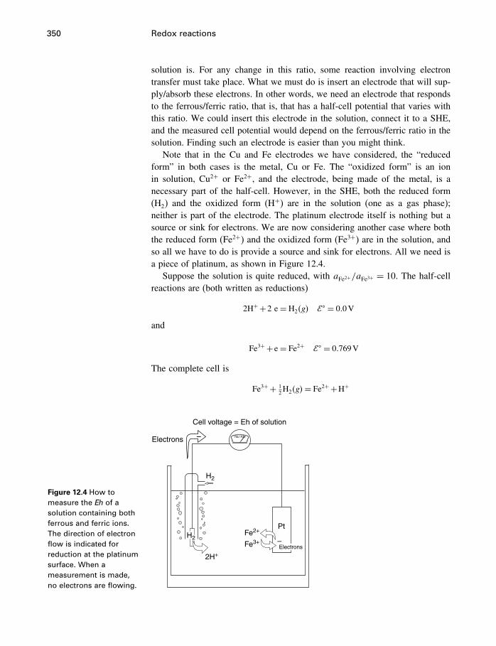
350 Redox reactions
solution is. For any change in this ratio, some reaction involving electrontransfer must take place. What we must do is insert an electrode that will sup-ply/absorb these electrons. In other words, we need an electrode that respondsto the ferrous/ferric ratio, that is, that has a half-cell potential that varies withthis ratio. We could insert this electrode in the solution, connect it to a SHE,and the measured cell potential would depend on the ferrous/ferric ratio in thesolution. Finding such an electrode is easier than you might think.
Note that in the Cu and Fe electrodes we have considered, the “reducedform” in both cases is the metal, Cu or Fe. The “oxidized form” is an ionin solution, Cu2+ or Fe2+, and the electrode, being made of the metal, is anecessary part of the half-cell. However, in the SHE, both the reduced form(H2) and the oxidized form (H+) are in the solution (one as a gas phase);neither is part of the electrode. The platinum electrode itself is nothing but asource or sink for electrons. We are now considering another case where boththe reduced form (Fe2+) and the oxidized form (Fe3+) are in the solution, andso all we have to do is provide a source and sink for electrons. All we need isa piece of platinum, as shown in Figure 12.4.
Suppose the solution is quite reduced, with aFe2+/aFe3+ = 10. The half-cellreactions are (both written as reductions)
2H++2 e= H2�g� �� = 0�0V
and
Fe3++ e= Fe2+ �� = 0�769V
The complete cell is
Fe3++ 12H2�g�= Fe2++H+
Figure 12.4 How tomeasure the Eh of asolution containing bothferrous and ferric ions.The direction of electronflow is indicated forreduction at the platinumsurface. When ameasurement is made,no electrons are flowing.
–
–
Cell voltage = Eh of solution
Electrons
Electrons
H2
2H+
H2
Fe2+
Fe3+
Pt
12.8 Measuring redox conditions 351
The Nernst equation may be written for either the complete cell or the Fehalf-cell, giving the same answers. Thus
� = Eh= �� − 0�059161
logaFe2+
aFe3+
= 0�769−0�05916× log�10�
= 0�710V
So the Eh of this relatively reduced solution is 0�710V. If the solution is quiteoxidized, with aFe2+/aFe3+ = 0�1,
� = Eh= �� − 0�059161
logaFe2+
aFe3+
= 0�769−0�05916× log�0�1�
= 0�828V
and the Eh of this more oxidized solution is 0�828V.To summarize, you may think of Eh of a solution as either a cell potential
or a half-cell potential. It is the potential of a cell having one electrode thatresponds reversibly to a redox couple (such as Fe2+/Fe3+) or couples in thesolution and the SHE as the other electrode. Or it is the half-cell potential ofan electrode responding reversibly to a redox couple or couples in the solution.You may use any kind of electrode as the other side of the cell, as long asyou correctly deduce the half-cell potential of the electrode that is respondingto conditions in your solution. Half-cell potentials are defined in terms of theSHE by our IUPAC conventions.
Therefore, we have an index of redox conditions, only assuming that reducedand oxidized species in solution can readily exchange electrons at a plat-inum surface. There are some practical difficulties in this respect, as discussedbelow.
12.8.2 Redox couples other than iron
But suppose our sample solution in Figure 12.4 contains not only the fer-rous/ferric redox couple, but also Mn2+–Mn4+, H2S–SO
2−4 , CH4–CO2, and
others. Even if all these redox couples are at equilibrium, each will have adifferent activity ratio. To which does our platinum electrode respond? Intheory, it responds to all of them simultaneously, and all result in the sameEh. Each couple has a different activity ratio, but each also has a differentvalue of ��, and the resulting Eh for the solution must be the same for eachredox couple if they are at equilibrium, and if each reacts with the platinumelectrode.
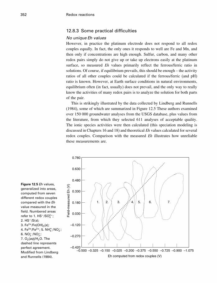
352 Redox reactions
12.8.3 Some practical difficulties
No unique Eh valuesHowever, in practice the platinum electrode does not respond to all redoxcouples equally. In fact, the only ones it responds to well are Fe and Mn, andthen only if concentrations are high enough. Sulfur, carbon, and many otherredox pairs simply do not give up or take up electrons easily at the platinumsurface, so measured Eh values primarily reflect the ferrous/ferric ratio insolutions. Of course, if equilibrium prevails, this should be enough – the activityratios of all other couples could be calculated if the ferrous/ferric (and pH)ratio is known. However, at Earth surface conditions in natural environments,equilibrium often (in fact, usually) does not prevail, and the only way to reallyknow the activities of many redox pairs is to analyze the solution for both partsof the pair.
This is strikingly illustrated by the data collected by Lindberg and Runnells(1984), some of which are summarized in Figure 12.5 These authors examinedover 150 000 groundwater analyses from the USGS database, plus values fromthe literature, from which they selected 611 analyses of acceptable quality.The ionic species activities were then calculated (this speciation modeling isdiscussed in Chapters 16 and 18) and theoretical Eh values calculated for severalredox couples. Comparison with the measured Eh illustrates how unreliablethese measurements are.
Figure 12.5 Eh values,generalized into areas,computed from sevendifferent redox couplescompared with the Eh
value measured in thefield. Numbered areasrefer to 1. HS−/SO2−
4 ;2. HS−/S(s);3. Fe2+/Fe�OH�3�s�;4. Fe3+/Fe2+; 5. NH+
4 /NO−2 ;
6. NO−2 /NO−
3 ;7. O2�aq�/H2O. Thedashed line representsperfect agreement.Modified from Lindbergand Runnells (1984).
–0.500 –0.325 –0.150 –0.025 –0.200 –0.375 –0.550 –0.725 –0.900 –1.075
Eh computed from redox couples (V)
0.780
0.630
0.480
0.330
0.180
0.030
–0.120
–0.270
–0.420
Fie
ld-m
easu
red
Eh
(V)
1. 2. 3. 4. 5. 6. 7.
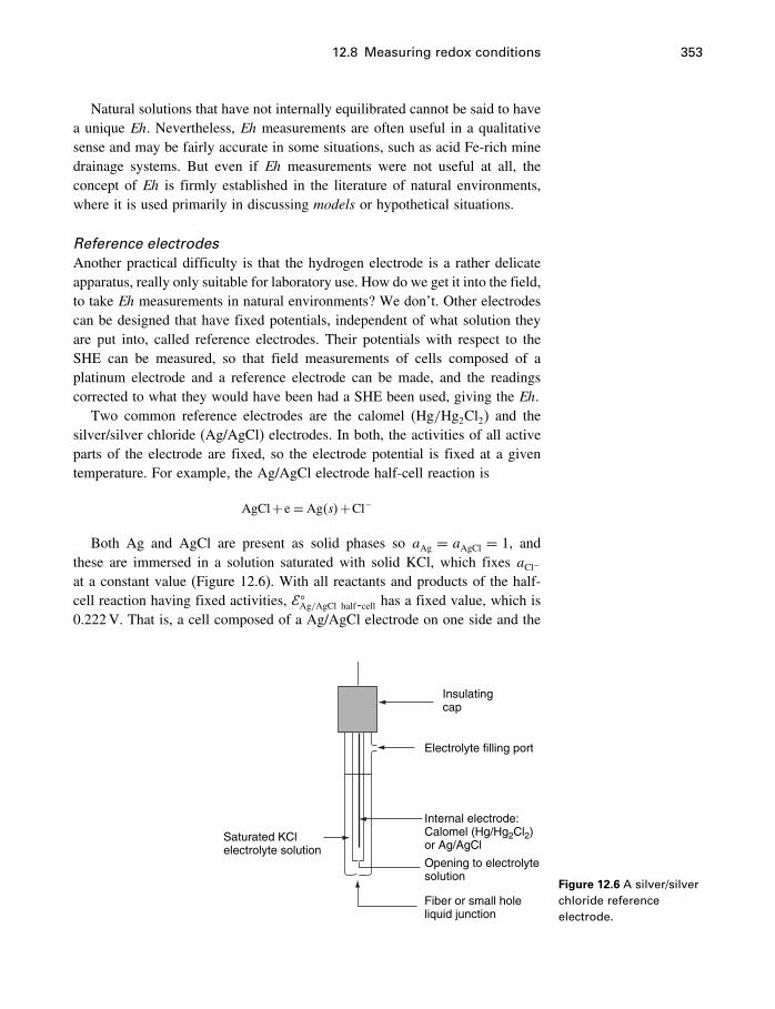
12.8 Measuring redox conditions 353
Natural solutions that have not internally equilibrated cannot be said to havea unique Eh. Nevertheless, Eh measurements are often useful in a qualitativesense and may be fairly accurate in some situations, such as acid Fe-rich minedrainage systems. But even if Eh measurements were not useful at all, theconcept of Eh is firmly established in the literature of natural environments,where it is used primarily in discussing models or hypothetical situations.
Reference electrodesAnother practical difficulty is that the hydrogen electrode is a rather delicateapparatus, really only suitable for laboratory use. How do we get it into the field,to take Eh measurements in natural environments? We don’t. Other electrodescan be designed that have fixed potentials, independent of what solution theyare put into, called reference electrodes. Their potentials with respect to theSHE can be measured, so that field measurements of cells composed of aplatinum electrode and a reference electrode can be made, and the readingscorrected to what they would have been had a SHE been used, giving the Eh.
Two common reference electrodes are the calomel (Hg/Hg2Cl2) and thesilver/silver chloride (Ag/AgCl) electrodes. In both, the activities of all activeparts of the electrode are fixed, so the electrode potential is fixed at a giventemperature. For example, the Ag/AgCl electrode half-cell reaction is
AgCl+ e= Ag�s�+Cl−
Both Ag and AgCl are present as solid phases so aAg = aAgCl = 1, andthese are immersed in a solution saturated with solid KCl, which fixes aCl−at a constant value (Figure 12.6). With all reactants and products of the half-cell reaction having fixed activities, ��
Ag/AgCl half-cell has a fixed value, which is0.222V. That is, a cell composed of a Ag/AgCl electrode on one side and the
Insulatingcap
Electrolyte filling port
Internal electrode:Calomel (Hg/Hg2Cl2)or Ag/AgCl
Opening to electrolytesolution
Fiber or small holeliquid junction
Saturated KClelectrolyte solution
Figure 12.6 A silver/silverchloride referenceelectrode.
354 Redox reactions
SHE on the other will record a constant potential of 0.222V. When used as areference electrode, immersed in a solution containing ferrous and ferric ionsand connected to a platinum electrode, for example, the cell reaction is
Fe3++Ag�s�+Cl− = Fe2++AgCl
and the standard cell potential of this cell is
�� = ��Fe2+/Fe3+ −��
Ag/AgCl
= 0�769−0�222
= 0�547V
whereas if measured against SHE, ��Fe2+/Fe3+ is 0�769V. Eh measurements are
defined as observed cell voltages using the SHE as reference, so if Ag/AgCl isused instead, 0.222V must be added (0�547+0�222= 0�769) to the observedreadings. For calomel reference electrodes, 0.268V must be added.
12.9 Eh–pH diagrams
The only other intensive variable of comparable significance in aqueous systemsis pH. It too is a function of the bulk composition at a given T and P, butboth are closely related to a large number of important reactions. Therefore,it proves natural to use both as variables in diagrams of systems at fixed Tand P, and Eh–pH diagrams have become a standard method of displayingand interpreting geochemical data. In the following sections we outline thetheoretical basis for calculating these diagrams.
In this section, we will calculate portions of a simple Eh–pH diagram forthe system Mn–H2O. This illustrates most of the problems encountered incalculating such diagrams. If you wish to add components such as CO2 or H2S,the methods are similar, and details are provided by Garrels and Christ (1965).
12.9.1 General topology of Eh–pH diagrams
First, let us examine the completed Eh–pH diagram for Mn–H2O–O2 inFigure 12.7. There are typically four different types of boundaries shown onthese diagrams. The top line, labeled O2/H2O, represents conditions for waterin equilibrium with O2 gas at 1 atm. Above this line, a PO2
greater than 1 atm isrequired for water to exist, so that because the diagram is drawn for a pressureof 1 atm, water is not stable above this line. Similarly, the bottom line H2O/H2
represents conditions for water in equilibrium with H2 gas at 1 atm. Below thisline, PH2
values greater than 1 atm are required for water to exist, that is, at1 atm water is not stable. Therefore, the water stability field is between thesetwo lines.
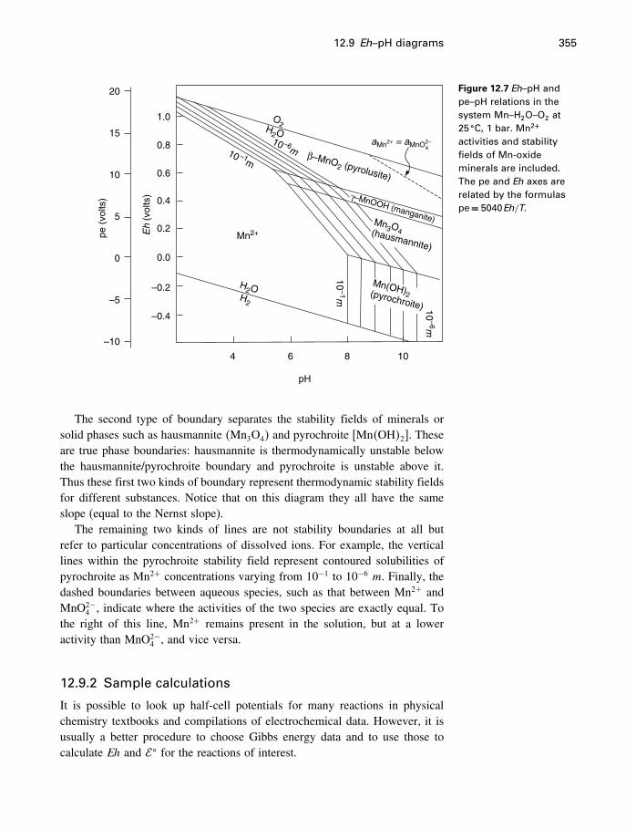
12.9 Eh–pH diagrams 355
20
1.0
0.8
0.6
0.4
0.2
0.0
–0.2
–0.4
15
10
5
0
–5
–10
pe (
volts
)
Eh
(vol
ts)
4 6 8 10
pH
10 –1m
Mn2+
H2O
H2
O2H
2O
10–1m
10–6m
10 –6m
Mn(OH)2(pyrochroite)
Mn3O4(hausmannite)
γ–MnOOH (manganite)
β–MnO2 (pyrolusite)
aMn2+ = aMnO2–4
Figure 12.7 Eh–pH andpe–pH relations in thesystem Mn–H2O–O2 at25 �C, 1 bar. Mn2+
activities and stabilityfields of Mn-oxideminerals are included.The pe and Eh axes arerelated by the formulaspe= 5040Eh/T�
The second type of boundary separates the stability fields of minerals orsolid phases such as hausmannite �Mn3O4� and pyrochroite �Mn�OH�2�. Theseare true phase boundaries: hausmannite is thermodynamically unstable belowthe hausmannite/pyrochroite boundary and pyrochroite is unstable above it.Thus these first two kinds of boundary represent thermodynamic stability fieldsfor different substances. Notice that on this diagram they all have the sameslope (equal to the Nernst slope).
The remaining two kinds of lines are not stability boundaries at all butrefer to particular concentrations of dissolved ions. For example, the verticallines within the pyrochroite stability field represent contoured solubilities ofpyrochroite as Mn2+ concentrations varying from 10−1 to 10−6 m. Finally, thedashed boundaries between aqueous species, such as that between Mn2+ andMnO2−
4 , indicate where the activities of the two species are exactly equal. Tothe right of this line, Mn2+ remains present in the solution, but at a loweractivity than MnO2−
4 , and vice versa.
12.9.2 Sample calculations
It is possible to look up half-cell potentials for many reactions in physicalchemistry textbooks and compilations of electrochemical data. However, it isusually a better procedure to choose Gibbs energy data and to use those tocalculate Eh and �� for the reactions of interest.
356 Redox reactions
As the first example, we will calculate the two boundaries for the stabilityfield of water.
For the boundary H2O�l�–O2�g�, the half-cell reduction reaction is
4H++O2�g�+4 e= 2H2O�l� (12.15)
for which n = 4. Using the tabulated �fG� for water (all others being zero),
we find
�rG� = 2�−237�129�−0
=−474�258 kJmol−1 (12.16)
Because
�rG� = −n� ��
then
�� = −�−474258/4×96485�
= 1�23V
From the Nernst equation (12.14)
Eh= �� −2�30259RT
n�log�1/�fO2
·a4H+��
Setting fO2= 1 atm, and recalling that pH=− logaH+ , gives the equation for
the boundary in terms of Eh and pH.
Eh= 1�23−0�0592pH (12.17)
For the boundary H2�g�–H2O�l�,
2H++2 e= H2�g�
�rG� = 0
=−n� ��
and
Eh= 0−2�30259RT
n�log�fH2
/a2H+�
or, with fH2= 1 atm, and n= 2�
Eh=−0�0592pH (12.18)
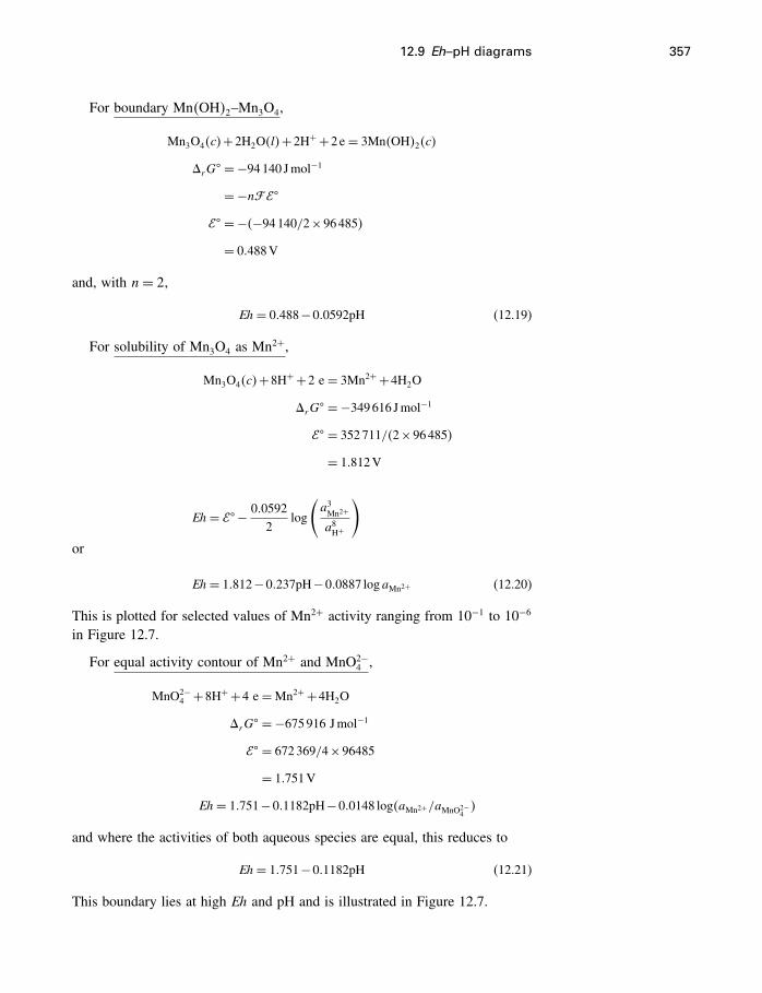
12.9 Eh–pH diagrams 357
For boundary Mn�OH�2–Mn3O4,
Mn3O4�c�+2H2O�l�+2H++2 e= 3Mn�OH�2�c�
�rG� = −94140 Jmol−1
=−n� ��
�� = −�−94140/2×96485�
= 0�488V
and, with n= 2�
Eh= 0�488−0�0592pH (12.19)
For solubility of Mn3O4 as Mn2+,
Mn3O4�c�+8H++2 e= 3Mn2++4H2O
�rG� = −349616 Jmol−1
�� = 352711/�2×96485�
= 1�812V
Eh= �� − 0�05922
log
(a3Mn2+
a8H+
)or
Eh= 1�812−0�237pH−0�0887 logaMn2+ (12.20)
This is plotted for selected values of Mn2+ activity ranging from 10−1 to 10−6
in Figure 12.7.
For equal activity contour of Mn2+ and MnO2−4 ,
MnO2−4 +8H++4 e=Mn2++4H2O
�rG� = −675916 Jmol−1
�� = 672369/4×96485
= 1�751V
Eh= 1�751−0�1182pH−0�0148 log�aMn2+/aMnO2−4�
and where the activities of both aqueous species are equal, this reduces to
Eh= 1�751−0�1182pH (12.21)
This boundary lies at high Eh and pH and is illustrated in Figure 12.7.
358 Redox reactions
12.9.3 pe–pH diagrams
There is a second way of calculating the same kinds of diagrams using thealternative variable pe rather than Eh. Because this is another way of doingexactly the same thing, it could be argued that the new variable pe is unnec-essary and redundant. However, the pe and Eh scales differ numerically, andpe calculations are now used about as frequently as Eh. It is thus worthwhilediscussing the use of this second variable.
The idea was to have an analogy between pH, which refers to hydratedprotons, and pe, which would refer to hydrated electrons. Like the proton, theelectron is assigned a standard �fG
� = 0. Like pH, pe is defined in terms ofactivity:
pH=− logaH+
pe=− logae (12.22)
In fact the “p” notation is now widely used for various quantities. For example,equilibrium constants are sometimes given in terms of pK, where
pK =− logK
In other words if K = 10−6�37, then pK = 6�37.Consider a half-cell reaction
aA+n e= bBwhere, at equilibrium
K = abBaaA a
ne
and
logK = logabBaaA a
ne
= logabBaaA
−n logae
= logabBaaA
+npe
so
pe= 1nlogK− 1
nlog
abBaaA
When A and B are in their standard states of unit activity, the last term dropsout, and we define pe� as
pe� = 1nlogK
12.10 Oxygen fugacity 359
Combining equations, we get
pe= pe� − 1nlog
abBaaA
= pe� − 1nlogQ (12.23)
12.9.4 Comparison of pe and Eh
There is a simple, linear relationship between the two variables pe and Eh,which is evident in comparing the two defining equations:
Eh= �� −2�30259RT
n�logQ [12.14]
pe= pe� − 1nlogQ [12.23]
Hence (and noting that pe� = ��),
pe= Eh�� /2�30259RT�
= 5040Eh/T
= Eh/0�05916 at 298.15 K (12.24)
Thus, if you prefer, you can calculate Eh and convert to pe with Equa-tion (12.24), or vice versa. The relationship between the two scales is illustratedin Figure 12.7, where oxidation potential is plotted as both Eh and pe. AnEh–pH diagram looks exactly like a pe–pH diagram, except that the Y -axis isshifted by the factor 5040/T .
12.10 Oxygen fugacity
As mentioned in §12.8, there are two methods in common use to represent thesame fundamental variable – the oxidation state of a system. It is time to lookat the second method, oxygen fugacity. This is a convenient parameter becauseany reaction that involves a change in oxidation state (any redox reaction) canbe written so as to include oxygen as a reactant or product, whether or notoxygen is actually involved in the reaction. We gave an example in Chapter 9(§9.4.2) of the oxidation of magnetite (in which some of the iron occurs as Fe3+
and some as Fe2+) to hematite (in which all of the iron occurs as Fe3+). Thisreaction often occurs in systems which contain no oxygen molecules at all.Nevertheless, the calculated fO2
(10−68�40) for magnetite–hematite equilibriumis a perfectly valid thermodynamic parameter, and the redox reaction involvingO2�g�
6Fe2O3�s�= 4Fe3O4�s�+O2�g�
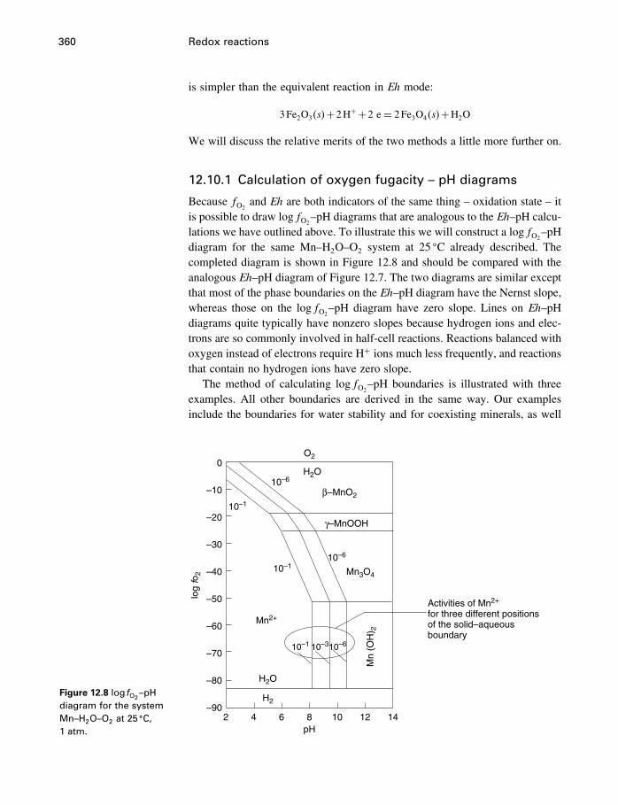
360 Redox reactions
is simpler than the equivalent reaction in Eh mode:
3Fe2O3�s�+2H++2 e= 2Fe3O4�s�+H2O
We will discuss the relative merits of the two methods a little more further on.
12.10.1 Calculation of oxygen fugacity – pH diagrams
Because fO2and Eh are both indicators of the same thing – oxidation state – it
is possible to draw logfO2–pH diagrams that are analogous to the Eh–pH calcu-
lations we have outlined above. To illustrate this we will construct a logfO2–pH
diagram for the same Mn–H2O–O2 system at 25 �C already described. Thecompleted diagram is shown in Figure 12.8 and should be compared with theanalogous Eh–pH diagram of Figure 12.7. The two diagrams are similar exceptthat most of the phase boundaries on the Eh–pH diagram have the Nernst slope,whereas those on the logfO2
–pH diagram have zero slope. Lines on Eh–pHdiagrams quite typically have nonzero slopes because hydrogen ions and elec-trons are so commonly involved in half-cell reactions. Reactions balanced withoxygen instead of electrons require H+ ions much less frequently, and reactionsthat contain no hydrogen ions have zero slope.
The method of calculating logfO2–pH boundaries is illustrated with three
examples. All other boundaries are derived in the same way. Our examplesinclude the boundaries for water stability and for coexisting minerals, as well
Figure 12.8 log fO2–pH
diagram for the systemMn–H2O–O2 at 25 �C,1 atm.
0
–10
–20
–30
–40
–50
–60
–70
–80
–90
10–1
10–6
10–1
10–1 10–310–6
10–6
Mn2+
β–MnO2
γ–MnOOH
Mn3O4
Mn
(OH
) 2
H2O
H2O
H2
2 4 6 8 10 12 14pH
log
fo2
O2
Activities of Mn2+
for three different positionsof the solid–aqueousboundary
12.10 Oxygen fugacity 361
as the aqueous solubility contours of a mineral. Notice that half-cell reactionsare not involved in these calculations.
For the water stability boundaries, the dissociation reaction of water is
2H2O= O2�g�+2H2�g� (12.25)
To calculate the equilibrium constant for this reaction,
�rG� = −2�−237129�
= 474258 Jmol−1
=−RT lnK
K = 10−83�1
= f 2H2fO2
(12.26)
The upper boundary occurs at 1 atm O2�g� pressure or logfO2= 0. The lower
boundary is at 1 atm H2�g� pressure; from the equilibrium constant (12.26),this corresponds to logfO2
= −83�1. As noted before, water can exist underconditions outside of these boundaries, but only if the pressure of oxygen orhydrogen is greater than 1 atm.
For the boundary Mn�OH�2–Mn3O4�,
12O2�g�+3Mn�OH�2 =Mn3O4+3H2O (12.27)
�rG� = −143093 Jmol−1
=−RT ln�1/f12O2�
Hence
logfO2=−50�14 (12.28)
For solubility of Mn3O4 as Mn2+,
3H2O�l�+3Mn2++ 12O2�g�=Mn3O4+6H+ (12.29)
�rG� = 114223 Jmol−1
=−RT ln
⎛⎜⎝ a6H+
f12O2a3Mn2+
⎞⎟⎠or
logfO2= 40−12pH−6 logaMn2+ (12.30)
This is plotted for selected values of Mn2+ activity ranging from 10−1 to 10−6
in Figure 12.8.
362 Redox reactions
12.10.2 Interrelating Eh, pH, and oxygen fugacity
The obvious similarity between the Eh–pH and logfO2–pH diagrams of
Figures 12.7 and 12.8 suggests that it should be possible to convert directlyfrom one set of coordinates to the other. This can be done using the half-cellreaction (12.15),
4H++O2�g�+4e= 2H2O�l� [12.15]
and its related Nernst equation,
Eh= �� − RT
n�ln�1/�fO2
a4H+�� (12.31)
This equation can be used to interrelate the three variables Eh, pH, and fO2�
The calculations are shown in §12.9.2, leading to an equation (12.17) for theEh of solutions having an fO2
of 1 atm. However, instead of 1 atm, we can justas easily insert any other fO2
value, leading to the more general relation
Eh= 1�23+0�0148 logfO2−0�0592pH (12.32)
Figure 12.9 shows Eh contours calculated from (12.32) drawn on a logfO2–
pH diagram, and logfO2contours on an Eh–pH diagram. The controlling factor
is the oxidation state of the system, which in turn is controlled by the bulkcomposition, and fO2
� fH2, Eh, pe, and all other related variables are simply
different ways of quantifying the same thing.
12.11 Redox reactions in organic chemistry
In inorganic reactions we think of hydrogen as always having valence of+1 (H+) and oxygen as always having valence −2 (O2−) and so we haveno difficulty in seeing that carbon in CH4 is C4−, and carbon in CO2 isC4+. But what is the oxidation state of carbon in octane, C8H18, or in aceticacid, CH3COOH, or in an enzyme containing hundreds of carbon, hydrogen,nitrogen, phosphorous, and other atoms? Applying our “normal” thinking tooctane, we get a “nominal” valence for carbon of 18/8 = 2�25. But how canan atom have a fractional valence? In acetic acid we get �−4+4�/2 = 0. Butone carbon in acetic acid is bonded to three hydrogens and one carbon, whilethe other is bonded partly to O and OH. Surely there is some difference in theelectron contributions of the two carbons. And in complex entities like largeproteins, the idea of counting up carbons and other atoms to get some nominaloxidation state becomes silly.
As pointed out by Helgeson (1991), it is quite possible to assign nominalcharge contribution of −1 for each C–H bond, zero for each C–C bond, and +1for each C–O, C–S, or C–N bond, and arrive at fractional valences that give aconsistent accounting of electron transfers in reactions, regardless of the actual
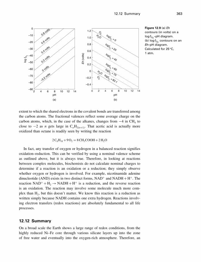
12.12 Summary 363
2 4 6 8 10 12 140
log
f O2
0
–10
–20
–30
–40
–50
–60
–70
–80
–902 4 6 8 10 12 14
pH pH
(a) (b)
1.2
1.0
0.8
0.6
0.4
0.2
0
–0.2
–0.4E
h (v
olts
)
0.8 volts
0.6 volts
0.4 volts
0.2 volts
0 volts
–0.2 volts O
2
O2
H2 O
H2 O
logfO2 = 0
logfO2 = 20
logfO2 = 40
logfO2 = 60logfO2 = 70logfO
2 = 83.1
Figure 12.9 (a) Ehcontours (in volts) on alog fO2
–pH diagram.(b) log fO2
contours on anEh–pH diagram.Calculated for 25 �C,1 atm.
extent to which the shared electrons in the covalent bonds are transferred amongthe carbon atoms. The fractional valences reflect some average charge on thecarbon atoms, which, in the case of the alkanes, changes from −4 in CH4 toclose to −2 as n gets large in CnH2�n+1�. That acetic acid is actually moreoxidized than octane is readily seen by writing the reaction
2C8H18+9O2 = 8CH3COOH+2H2O
In fact, any transfer of oxygen or hydrogen in a balanced reaction signifiesoxidation–reduction. This can be verified by using a nominal valence schemeas outlined above, but it is always true. Therefore, in looking at reactionsbetween complex molecules, biochemists do not calculate nominal charges todetermine if a reaction is an oxidation or a reduction; they simply observewhether oxygen or hydrogen is involved. For example, nicotinamide adeninedinucleotide (AND) exists in two distinct forms, NAD+ and NADH+H+. Thereaction NAD++H2 → NADH+H+ is a reduction, and the reverse reactionis an oxidation. The reaction may involve some molecule much more com-plex than H2, but this doesn’t matter. We know this reaction is a reduction aswritten simply because NADH contains one extra hydrogen. Reactions involv-ing electron transfers (redox reactions) are absolutely fundamental to all lifeprocesses.
12.12 Summary
On a broad scale the Earth shows a large range of redox conditions, from thehighly reduced Ni–Fe core through various silicate layers up into the zoneof free water and eventually into the oxygen-rich atmosphere. Therefore, an
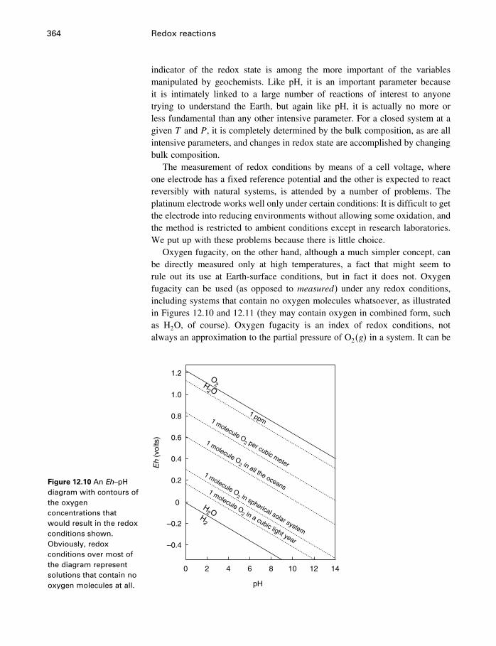
364 Redox reactions
indicator of the redox state is among the more important of the variablesmanipulated by geochemists. Like pH, it is an important parameter becauseit is intimately linked to a large number of reactions of interest to anyonetrying to understand the Earth, but again like pH, it is actually no more orless fundamental than any other intensive parameter. For a closed system at agiven T and P, it is completely determined by the bulk composition, as are allintensive parameters, and changes in redox state are accomplished by changingbulk composition.
The measurement of redox conditions by means of a cell voltage, whereone electrode has a fixed reference potential and the other is expected to reactreversibly with natural systems, is attended by a number of problems. Theplatinum electrode works well only under certain conditions: It is difficult to getthe electrode into reducing environments without allowing some oxidation, andthe method is restricted to ambient conditions except in research laboratories.We put up with these problems because there is little choice.
Oxygen fugacity, on the other hand, although a much simpler concept, canbe directly measured only at high temperatures, a fact that might seem torule out its use at Earth-surface conditions, but in fact it does not. Oxygenfugacity can be used (as opposed to measured) under any redox conditions,including systems that contain no oxygen molecules whatsoever, as illustratedin Figures 12.10 and 12.11 (they may contain oxygen in combined form, suchas H2O, of course). Oxygen fugacity is an index of redox conditions, notalways an approximation to the partial pressure of O2�g� in a system. It can be
Figure 12.10 An Eh–pHdiagram with contours ofthe oxygenconcentrations thatwould result in the redoxconditions shown.Obviously, redoxconditions over most ofthe diagram representsolutions that contain nooxygen molecules at all.
0 2 4 6 8 10 12 14
pH
1.2
1.0
0.8
0.6
0.4
0.2
0
–0.2
–0.4
Eh
(vol
ts)
O2H
2 O
H2 O
H2
1 ppm1 molecule O2 per cubic meter
1 molecule O2 in all the oceans
1 molecule O2 in spherical solar system
1 molecule O2 in a cubic light year
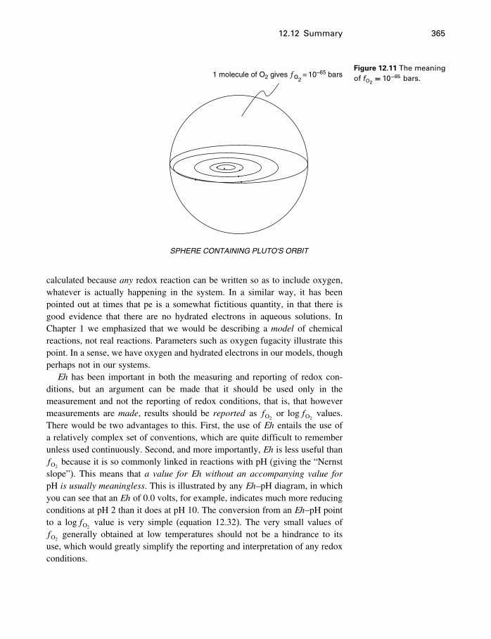
12.12 Summary 365
•
•
• •
••
1 molecule of O2 gives ƒo2= 10–65 bars
SPHERE CONTAINING PLUTO'S ORBIT
Figure 12.11 The meaningof fO2
= 10−65 bars.
calculated because any redox reaction can be written so as to include oxygen,whatever is actually happening in the system. In a similar way, it has beenpointed out at times that pe is a somewhat fictitious quantity, in that there isgood evidence that there are no hydrated electrons in aqueous solutions. InChapter 1 we emphasized that we would be describing a model of chemicalreactions, not real reactions. Parameters such as oxygen fugacity illustrate thispoint. In a sense, we have oxygen and hydrated electrons in our models, thoughperhaps not in our systems.Eh has been important in both the measuring and reporting of redox con-
ditions, but an argument can be made that it should be used only in themeasurement and not the reporting of redox conditions, that is, that howevermeasurements are made, results should be reported as fO2
or logfO2values.
There would be two advantages to this. First, the use of Eh entails the use ofa relatively complex set of conventions, which are quite difficult to rememberunless used continuously. Second, and more importantly, Eh is less useful thanfO2
because it is so commonly linked in reactions with pH (giving the “Nernstslope”). This means that a value for Eh without an accompanying value forpH is usually meaningless. This is illustrated by any Eh–pH diagram, in whichyou can see that an Eh of 0.0 volts, for example, indicates much more reducingconditions at pH 2 than it does at pH 10. The conversion from an Eh–pH pointto a logfO2
value is very simple (equation 12.32). The very small values offO2
generally obtained at low temperatures should not be a hindrance to itsuse, which would greatly simplify the reporting and interpretation of any redoxconditions.
13Equations of state
13.1 Introduction
In Chapter 10 we looked at some properties of solutions, derived as deviationsfrom ideal mixing. There was no thought of developing an equation for either(or any) of the substances being mixed, that is, an equation from which wecould calculate the properties of each individual compound or phase. If wecould do that, we might then extend that approach, and develop equations forthe properties of the mixtures. Such equations are equations of state (EoS), andrepresent a completely different approach to the same problem.
Establishing equations of state for widely occurring substances is a kind of“holy grail” for experimental and theoretical geochemists, because it encapsu-lates in a compact form all the thermodynamic information about a compoundor a system. In this section we consider only EoS for gases and supercriticalfluids, except that some EoS also provide the condensation conditions for thegas, i.e., information on the saturation equilibrium. Equations of state in com-pletely different forms also exist for solids and liquids, used extensively ingeophysics and astrophysics, but we will not consider these.
We begin by considering the case of the simplest possible substance, theideal gas.
13.2 The ideal gas
13.2.1 The ideal gas equation
Equations of state are commonly described as equations which relate the P, Vand T of a substance. The simplest example is the ideal gas equation,
V= nRTP
(13.1)
where n is the number of moles, or
V = RT
P(13.2)
366
13.2 The ideal gas 367
which expresses the early experimental results of Boyle, Charles, andGay-Lussac, and can also be derived from statistical mechanics. Thinking of(13.2) as a truncated virial equation is also useful as this immediately impliesthat it neglects all intermolecular forces, as we will see (§13.5). This equa-tion doesn’t work very well (is not very accurate) for real gases, especiallyat high pressures, but has served as the starting point for a variety of equa-tions which introduce adjustable variables, some of which we will describebelow.
13.2.2 Properties of the ideal gas
The thermodynamic properties of the hypothetical ideal gas are of practicalinterest because, as we will see (§13.2.3, §13.6.1) it is common practice indeveloping an equation for real systems to first subtract the properties of theideal gas, which are known, and then deal only with the deviations from theseproperties. The properties of the ideal gas are in many cases not quite as simpleas you might suppose.
Effect of pressureIt is fairly intuitive that many properties of the ideal gas should be independentof pressure, but not independent of temperature. If there is no interactionwhatsoever between molecules, which have zero volume, then it should notmatter how close together they are (the effect of P). But if we add heat to thegas (we raise the T ), that energy cannot disappear, but must be reflected in thethermodynamic properties of the ideal gas.
We can show this analytically without much effort too. In Equation (5.42)we indicated that the effect of pressure on the enthalpy of an ideal gas iszero. That this is also true for the effect of pressure on internal energy, wenote that (
�H
�P
)T
=(��U +PV�
�P
)T
=(��U +RT�
�P
)T
=(�U
�P
)T
(13.3)
From these relations it is not difficult to show that the effect of P on CP andCV is also zero.
On the other hand, Equation (5.41) shows that the effect of pressure on theentropy of ideal gas is not zero, and therefore pressure also affects the idealgas Gibbs and Helmholtz energies.
368 Equations of state
Effect of temperatureThe effect of temperature on internal energy is the same as its effect on enthalpy,because (
�H
�T
)P
=(��U +PV�
�T
)P
=(�U
�T
)P
= CP (13.4)
The heat capacity of an ideal gas depends on whether the gas is monatomic,diatomic, or whatever, and is derived through statistical mechanics, which wewill not go into. For the simplest case, a monatomic ideal gas,
CV =(�U
�T
)V
= 32R (13.5)
and because
CP −CV = R (13.6)
then
CP = 52R (13.7)
Despite the simplicity of these expressions for the heat capacity of amonatomic ideal gas, expressions for polyatomic molecules such as H2O canbecome quite complex. Of course H2O is not an ideal gas; the question iswhat is the heat capacity (and other heat capacity-dependent properties) of agas having molecules with the properties of the H2O molecule, but with nointermolecular forces? This is a nontrivial problem in statistical mechanics.For H2O, the results of Wooley (1980) are used. These were fit to an equationby Cooper (1982) which, after some rearranging, was used by Wagner andPruß (2002) in their equation of state for H2O (see below). This equation is asummation of simple harmonic oscillator functions, and is
CP
R= b0+
5∑i=1
bi��/T�2e−�i/T
�1− e−�i/T �2 (13.8)
where b and � are arrays of fit coefficients. Being an equation for heat capacity,it can be integrated to give expressions for Gibbs and Helmholtz energies, aswell as enthalpy.
You might reasonably ask at this point, why should we be interested in idealgas properties, especially when they get so complex, if we want to develop anequation for real gases? The reason is in the form of residual functions.
13.2 The ideal gas 369
13.2.3 Residual functions
Residual functions (MR) are defined as
MR =Mactual−M ideal gas (13.9)
where Mactual is any thermodynamic property of a real system, and M ideal gas isthat same property for that system behaving as an ideal gas under the sameconditions, either of T and P, or T and �.
Because the ideal gas has no intermolecular forces, the various parametersof the ideal gas (Gideal gas, H ideal gas, etc.) represent those parameters a real fluidwould have in the absence of such forces, and the residual functions thereforerepresent the contributions to those parameters when the intermolecular forcesare “turned on” (Prausnitz, et al., 1999, Appendix B). As such they find usein statistical mechanics and in the development of equations of state. Don’tconfuse residual functions with excess functions.
The functional forms of ideal gas properties and hence of residual functionsare well known. For example, the residual enthalpy is
HR =−RT 2∫ P
P0
(�Z
�T
)P
d lnP
the residual entropy is
SR = R∫ P
P0
{T
(�Z
�T
)P
+Z−1}d lnP
and so on, where Z is the compressibility factor (see below). Ewing andPeters (2000) give a complete list in terms of both (T�P) and (T��). However,knowing the form of the equation is only the beginning. You still have to knowhow to perform the integration, and this requires real data.
Fugacity coefficient as a residual functionWe should note that not only is a residual function (Equation 8.8), but so ina closely related sense is the fugacity coefficient f . We saw that the Gibbsenergy for an ideal gas can be written dGideal gas =RT d lnP (Equation 8.1), andthat for a real gas as dG= RT d ln f (Equation 8.4). So, if GR =G−Gideal gas
is the residual Gibbs energy,
dGR = dG−dGideal gas∫ P
P0
dGR =∫ P
P0
�RT d ln f −RT d lnP�
The lower limit of integration is zero on the left and cancels on the right, so
GR = RT lnf
P
= RT lnf (13.10)
370 Equations of state
Therefore the fugacity coefficient, in the form RT lnf , is a measure of theresidual Gibbs energy. Then from (8.13),
GR = RT∫ P
P0
�Z−1�d lnP (13.11)
which is a more common way of expressing this function (Ewing and Peters,2000).
13.2.4 The compressibility factor
J.D. van der Waals noticed, on empirical grounds, that
Z = PV
RT(13.12)
is the same for most gases, if the comparison is made when each gas has thesame relation to its critical point. This is the principle of corresponding states.If we define a “reduced temperature”
Tr = T/Tcwhere T is the gas temperature (in kelvins) and Tc is its critical temperature (inkelvins), and a “reduced pressure”
Pr = P/Pc
where P is the gas pressure and Pc is its critical pressure, then most gases haveabout the same Z at a given Pr, Tr, within certain ranges.
Since van der Waals pointed this out, there have been great advances inour understanding of the fluid state. However, for dense fluids (liquids) theseresults are quite complex. Ely and Marrucho (2000) point out that
With this complexity in mind, the most powerful tool available today (just as 25
years ago) for making highly accurate, yet mathematically simple, predictions
of the thermophysical properties of fluids and fluid mixtures is the
corresponding states principle.
and
… all modern generalized engineering equations of state are examples of
applications of this principle.
van der Waals would be pleased.The principle of corresponding states is a two-parameter theory and works
well only for “simple” molecules, which are the noble gases and a few nonpolaror very slightly polar ones. Two main approaches have been used in expandingits range of applicability. One is to introduce a third parameter, the mostsuccessful being the acentric factor, and the other is based on manipulating theintermolecular potentials. We will mention only the acentric factor.
13.4 Cubic equations of state 371
The acentric factorFor molecules more complex than the noble gases, a third parameter is intro-duced (Pitzer et al. 1955; Pitzer 1955) to form a three-parameter theory ofcorresponding states. This is the acentric factor �, which is a function of theacentricity or noncentral nature of the intermolecular forces. It is completelyempirical. For simple fluids, it was observed that at a reduced temperature of0.7, the saturation pressure (i.e., the vapor pressure of the liquid–gas equilib-rium) divided by the critical pressure is very close to 1/10, or
Ps
Pc= 1
10
where Ps is the saturation pressure. So the acentric factor was defined as
�=− log(Ps
Pc
)T/Tc=0�7
−1�0 (13.13)
making �= 0 for simple fluids. This modified theory of corresponding statesthen says that the properties of gases having the same reduced temperature,reduced pressure and acentric factor are the same.
13.3 Two kinds of EoS
It is important to realize that however valuable PVT information is (and itis extremely valuable in the chemical industries), it is not thermodynamicallycomplete information. You cannot calculate a heat capacity from PVT data,and this means that you cannot calculate the temperature variation of the Gibbsenergy, enthalpy, or entropy. You can calculate the pressure variation of thesefunctions, but you need to start with a baseline showing the variation with Tat some pressure. There is a second important class of EoS, sometimes called“thermal EoS,” which do provide complete information, and these are equationsbased on G�T�P� or A�T�V�. We will look first at PVT equations of state.
Apart from the ideal gas equation, equations relating P, V , and T are usuallycubic equations.
13.4 Cubic equations of state
13.4.1 The van der Waals equation
The ideal gas law does not work well for real gases at even moderate pressures.Two of its main problems were recognized by van der Waals, and appropriatecorrections were incorporated into his famous equation of state of 1873:
P = RT
V −b︸ ︷︷ ︸repulsion
− a
V 2︸︷︷︸attraction
(13.14)
372 Equations of state
where a and b are experimentally derived constants, different for each gaseouscompound. The quantity V −b corrects for the volume occupied by moleculesof finite volume (molecules of an ideal gas are supposed to be vanishinglysmall). The parameter b is called the excluded volume per mole, since thevolume available for movement of any one molecule is V minus the volumeb of all other molecules in the same space. This crowding raises the pressurerelative to an ideal gas according to P=RT/�V−b�. The second term in (13.14)corrects for intermolecular attractions. The forces between all gas moleculessomewhere in the center of a container should be the same in all directions, onthe average. However, the average forces on molecules at the outer wall of thecontainer are directed inward; this must reduce the pressure exerted by theseoutermost molecules on the wall.
The concentration of the outermost zone of molecules is proportional to thegas density 1/V , as is the concentration of molecules in the next inward zone(presuming concentrations in both zones are the same – a potential source oferror). The inward attraction is proportional to the number of molecules in bothzones or to 1/V 2. Introducing the proportionality constant a, this inward pullshould modify the outward force or pressure by −a/V 2.
The van der Waals equation fits the PVT behavior of real gases betterthan the ideal gas law, but still fails at moderate to high pressures whereintermolecular forces are stronger. We would expect it to work a little betterfor two reasons: First, it is based on a simplistic, but not unreasonable physicalpicture of a real gas and should therefore have an appropriate mathematicalshape. Second, it contains two adjustable parameters a and b which can befitted to data by regression analysis or other procedures. This gives it flexibilityand “personalizes” it for different gases.
The first cubic EoSBut these two correction factors have one other extremely important effect –they transform the simple linear ideal gas equation into a cubic equation. Thisis perhaps not obvious from the usual presentation in Equation (13.14), butrewriting this as
V 3−(b+ RT
P
)V 2+ a
PV − ab
P= 0 (13.15)
shows that it is in fact a cubic equation in V . This means that solving theequation for V will produce three roots. The wonderful thing is that giventhe values of a and b for some gas, solving for V as a function of P willproduce one real root and two imaginary roots above and below a certain valueof P, and three real, positive roots within a very narrow range of P values.A simple calculation (found by Maxwell in 1875) is used to determine the exactpressure within this range. This pressure represents the two-phase gas–liquidsaturation state of the gas. Of the three real roots, the smallest is interpreted
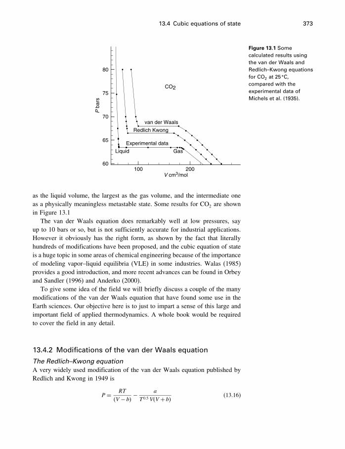
13.4 Cubic equations of state 373
V cm3/mol
Pba
rs
100 20060
65
70
75
80
van der Waals
Redlich Kwong
Experimental data
CO2
GasLiquid
Figure 13.1 Somecalculated results usingthe van der Waals andRedlich–Kwong equationsfor CO2 at 25 �C,compared with theexperimental data ofMichels et al. (1935).
as the liquid volume, the largest as the gas volume, and the intermediate oneas a physically meaningless metastable state. Some results for CO2 are shownin Figure 13.1
The van der Waals equation does remarkably well at low pressures, sayup to 10 bars or so, but is not sufficiently accurate for industrial applications.However it obviously has the right form, as shown by the fact that literallyhundreds of modifications have been proposed, and the cubic equation of stateis a huge topic in some areas of chemical engineering because of the importanceof modeling vapor–liquid equilibria (VLE) in some industries. Walas (1985)provides a good introduction, and more recent advances can be found in Orbeyand Sandler (1996) and Anderko (2000).
To give some idea of the field we will briefly discuss a couple of the manymodifications of the van der Waals equation that have found some use in theEarth sciences. Our objective here is to just to impart a sense of this large andimportant field of applied thermodynamics. A whole book would be requiredto cover the field in any detail.
13.4.2 Modifications of the van der Waals equation
The Redlich–Kwong equationA very widely used modification of the van der Waals equation published byRedlich and Kwong in 1949 is
P = RT
�V −b� −a
T 0�5 V�V +b� (13.16)
374 Equations of state
As you can see, this retains the first term of the van der Waals equation butmodifies the second term.
Since the RK equation first appeared, it too has undergone many modifica-tions in an attempt to further improve its ability to fit data for gases. Many ofthese modified Redlich–Kwong equations are summarized by Holloway (1977)and Kerrick and Jacobs (1981), and involve writing the a and b parameters asa function of T and/or P. The MRK equation of Kerrick and Jacobs keeps bconstant but writes a as a function of both P and T :
P = RT�1+y+y2−y3�V�1−y�3 − a�P�T�
T 0�5V�V +b� (13.17)
Redlich–Kwong and van der Waals equations
For CO2, Tc = 304�21K, Pc = 73�285 bars, and at 298.15K Equations (13.19)
and (13.20) give a= 3655953 and b = 42�8269.
Solving Equations (13.14) and (13.16) for V as a function of P gives the following
results:
van der Waals Redlich–Kwong
P, bars V� cm3 mol−1 P, bars V� cm3 mol−1
60 260.5* 60 240.5*
61 251.4* 61 231.0*
62 242.3* 62 221.3*
63 233.0* 63 211.4*
64 223.6* 64 201.0, 100.0, 86.4
65 213.8* 65 189.8, 109.0, 82.6
66 203.4* 66 176.8, 118.4, 80.4
67 106.2, 114.6, 192.0 67 168.9, 124.3, 79.5
68 99.9, 129.5, 177.9 68 77.5*
69 97.1* 69 76.3*
70 95.1* 70 75.4*
80 85.9* 80 69.4*
* indicates there are two additional complex roots
These results are plotted in Figure 13.1, but only one liquid–gas equilibrium
pressure is shown.
Note: If you solve these equations, or any cubic, using a spreadsheet solver, only
one root is reported. To see all three roots you must use one of the analytical
methods, or a program such as Mathematica or Maple.
13.4 Cubic equations of state 375
where
y = b/4V �b is constant)
a�P�T�= c�T�+d�T�/V + e�T�/V 2
z�T�= z1+ z2T + z3T 3 (where z is c, d, or e)�
Here you can see that the repulsion term holds b constant but is morecomplicated (which gives it better flexibility). The a parameter in the attractionterm is written as a simple polynomial function of 1/V (hence of P) and of T .This is a MRK equation with 10 adjustable parameters, so naturally it fits realdata considerably better than the original RK equation, which has only twoparameters.
The Peng–Robinson equationPeng and Robinson (1976) proposed the equation
P = RT
V −b −a
V�V +b�+b�V −b� (13.18)
with
a= �0�457235R2T 2c /Pc�
b = 0�077796RTc/Pc
= �1+��1−T 0�5r ��2
where Tr is the reduced temperature (§13.2.4), and � is a function of theacentric factor.
This equation is widely used for hydrocarbons and some nonhydrocarbongases such as CO2 and N2, but does not work very well for H2O and otherpolar gases. It too has had many modifications, such as those of Stryjek andVera (1986a,b,c), which greatly improves the results for polar compounds(PRSV equation). This improvement was made, in Stryjek and Vera (1955c),by modifying � to
�= �0+ ��1+�2��3−Tr��1−T 0�5r ���1+T 0�5
r ��0�7−T 0�5r �
where
�0 = 0�378893+1�4897153�−0�17131848�2+0�0196544�3
and �1, �2, and �3 are adjustable parameters for each compound.This equation proved useful to Suleimenov and Krupp (1994) in their study
of the important system H2S−H2O. Stryjek and Vera (1986b, c) also proposedmixing rules for the use of the PRSV equation with mixtures of gases (§13.4.4).

376 Equations of state
13.4.3 Estimating EoS parameters from criticalconditions
The a and b parameters in the RK and van der Waals class of equations arebest estimated from a regression fit to an overall PVT data set for a gas.However, there is a much quicker way of estimating the same parametersbased on the critical behavior of the gas. If these critical data are knownwith sufficient accuracy and precision, the estimates should be very good,and this approach is used quite frequently when the utmost accuracy is notrequired.
The first and second derivatives of the critical isotherm must both be zeroat the critical point. The van der Waals equation itself should also work at thecritical point, so we can write the three following equations:
Pc =RTcVc−b
− a
V 2c
��P/�V�Tc = 0= −RTc�Vc−b�2
+ 2aV 3c
��2P/�V 2�Tc = 0= 2RTc�Vc−b�3
− 6aV 4c
Solving these three equations for the critical constants gives
Tc = 8a/27bR
Vc = 3b
Pc = a/27b2
and solving for the van der Waals parameters, we find
a= 3PcV2c
= 27R2T 2c
64Pc(13.19)
b = Vc/3
= RTc8Pc
(13.20)
where
Vc = 3RTc/8Pc
We can apply exactly the same reasoning to the RK equation (13.16) andobtain
aRK = 0�427480R2T 2�5c /Pc
bRK = 0�086640RTc/Pc
13.4 Cubic equations of state 377
Thus the a and b constants in both the van der Waals and the RK equationscan be calculated quite easily given sufficiently good data on the criticaltemperature and pressure of a fluid. Alternatively, you can calculate the criticalconditions for a gas directly from the a and b parameters for either equation ofstate.
13.4.4 EoS for mixtures – mixing rules
A natural question to ask is how these equations might be applied to mixtures ofgases. To use the van der Waals equation (13.2) or any of its modifications, thea and b parameters must be known for each pure component. If no experimentaldata are available for a mixture of these components, how do we get valuesof a and b that could apply to the mixture? Many so-called mixing rules havebeen devised to do this (see, for example, Prausnitz et al. 1999), but the mostpopular remain those originally suggested by van der Waals. Since the repulsiveb parameter is supposed to be a measure of the volume of the molecules, asimple averaging over all m different gas species might work:
bmix�x1� x2� �=m∑j=1
xjbj (13.21)
The a (molecular attraction) parameter for the mixture is obtained by averagingover all possible kinds of molecular pairs:
amix�x1� x2� �=m∑j=1
m∑k=1
xjxkajk (13.22)
where
ajk = �ajak�0�5 (13.23)
In (13.22) and (13.23), ajk is supposed to describe the interaction between onemolecule of type j and another of type k. For j = k, ajk = ajj and is simply thevan der Waals a parameter for the pure gas j. The problem is how to find aterm ajk�j �= k� for the interaction between unlike molecules when there are nodata on the mixture itself. Berthelot suggested the geometric mean assumptionof Equation (13.23) on strictly empirical grounds, and it was used by van derWaals in his own work on gas mixtures. For some cases this assumption canbe theoretically justified, but why it works is still a bit of a mystery. As canbe imagined, there has been much discussion and controversy over this point,and equations for mixing rules can become quite complex.
A completely different approach to mixing rules is the “one fluid” model, inwhich it is not a and b which are modified, but the intermolecular potentials.We have a look at this method in §13.7.1.
378 Equations of state
13.5 The virial equation
In 1901 Kammerlingh-Onnes first used a power series to describe the PVTproperties of a gas.1 This is now known as a virial equation of state, and canbe written in various related ways:
PV
RT= 1+ B
V+ C
V 2+ D
V 3+· · · (13.24)
or, because V = 1/�,
P
RT= �+B�2+C�3+D�4+· · · (13.25)
Often it is more convenient to use P and T as variables, in which case theequation becomes
PV
RT= Z
= 1+B′P+C ′P2+D′P3+· · · (13.26)
The coefficients of the terms in P or 1/V are known as virial coefficients. Thecoefficients in the pressure form of Equation (13.26) are related to those inthe volume or � form by B′ = B/RT and C ′ = �C−B2�/�RT�2. If (13.26) iswritten
PV = RT +B′P+C ′P2+D′P3+· · · (13.27)
then B′ = B, and C ′ = �C−B2�/RT .At first sight this looks like nothing more than a polynomial expansion of the
ideal gas law. However, it turns out to have real physical significance. Statisticalmechanics shows that the second coefficient arises from the interaction of pairsof molecules, the third from the interaction of molecules three at a time, andso on. They can be calculated from known interaction potentials, or used toestimate such potentials from observed PVT behavior. The details can be foundin most textbooks on statistical mechanics (for example McQuarrie, 2000,Chapter 12), and Prausnitz et al. (1999) give an extensive treatment of variouscommonly used formulations of these intermolecular forces and their use inequations of state.
Because it is an equation of state, it (at least in principle) allows calculationof all thermodynamic parameters. For example, chemical potentials in terms ofvirial parameters are (starting with (13.25))
�−�� = RT ln ��RT�+2B�+ 3C ′�2
2+ 4D′�3
3+· · · (13.28)
1 Kammerlingh-Onnes, a colleague of van der Waals, is possibly better known for liquefyinghelium in 1908, discovering superconductivity in 1911, and receiving the Nobel Prize inPhysics in 1913.
13.5 The virial equation 379
Other examples will be cited later on. For a complete summary, see Pitzer(1995, p. 133).
The virial equation approach has also been used for providing an equation ofstate for aqueous solutes, including electrolytes. In the 1970s, Kenneth Pitzerand his associates developed such equations, which have proven to be quitesuccessful at fitting the behavior of both single- and mixed-salt solutions to highconcentrations. This will be treated in more detail in §13.6.3 and Chapter 15.
13.5.1 Fugacities from virial equations
For a pure phase, we can rewrite Equation (13.26) as
Z−1= B′P+C ′P2+D′P3+· · · (13.29)
and combining this (omitting the D′ term) with (8.13), we get
lnf =∫ P
P0
�B′P+C ′P2�d lnP
=∫ P
P0
B′P+C ′P2
PdP
= B′P+ 12C
′P2 (13.30)
where the terms referring to the lower limit of integration (P0) drop out, becauseP0 is very small, theoretically zero. Also note that (13.30) is also the residualGibbs energy GR/RT , from (13.10). From this you can see that in fact allresidual thermodynamic properties are also easily expressed in terms of virialcoefficients. A complete list is given by Trusler (2000).
The same equations are used for mixtures of gases. In this case the coeffi-cients are combinations of the coefficients of the pure components. They arecombined according to “mixing rules,” which are also specified by statisticalmechanics for any number of components. The second virial coefficient is, fora mixture of m components,
Bmix =m∑i=1
m∑j=1
xixjBij (13.31)
which, for a binary system with components 1 and 2 becomes (becauseB12 = B21)
Bmix = x21B11+2x1x2B12+x22B22 (13.32)
so there are in fact three second virial coefficients, which require experimentaldata for three systems – pure 1, pure 2, and mixtures of 1 and 2. The thirdcoefficient is given by
Cmix =m∑i=1
m∑j=1
m∑k=1
xixjxkCijk (13.33)
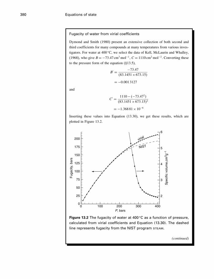
380 Equations of state
Fugacity of water from virial coefficients
Dymond and Smith (1980) present an extensive collection of both second and
third coefficients for many compounds at many temperatures from various inves-
tigators. For water at 400 �C, we select the data of Kell, McLaurin and Whalley,
(1968), who give B=−73�47cm3 mol−1, C = 1110 cm2 mol−2. Converting these
to the pressure form of the equation (§13.5),
B′ = −73�47�83�1451×673�15�
=−0�0013127
and
C ′ = 1110− �−73�472��83�1451×673�15�2
=−1�36881×10−6
Inserting these values into Equation (13.30), we get these results, which are
plotted in Figure 13.2.
P, bars
Fug
acity
, bar
s
Spe
cific
vol
ume,
cm3 g
–1
0 100 200 300 4000
25
50
75
100
125
150
175
200
2
3
4
5
6
virial
NIST
Figure 13.2 The fugacity of water at 400 �C as a function of pressure,calculated from virial coefficients and Equation (13.30). The dashedline represents fugacity from the NIST program steam.
(continued)
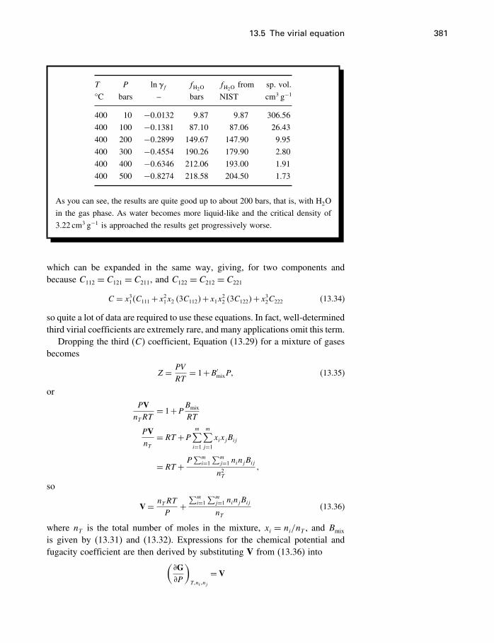
13.5 The virial equation 381
T P lnf fH2OfH2O
from sp. vol.
°C bars – bars NIST cm3 g−1
400 10 −0�0132 9.87 9.87 306.56
400 100 −0�1381 87.10 87.06 26.43
400 200 −0�2899 149.67 147.90 9.95
400 300 −0�4554 190.26 179.90 2.80
400 400 −0�6346 212.06 193.00 1.91
400 500 −0�8274 218.58 204.50 1.73
As you can see, the results are quite good up to about 200 bars, that is, with H2O
in the gas phase. As water becomes more liquid-like and the critical density of
3.22 cm3 g−1 is approached the results get progressively worse.
which can be expanded in the same way, giving, for two components andbecause C112 = C121 = C211, and C122 = C212 = C221
C = x31�C111+x21x2 �3C112�+x1x22 �3C122�+x32C222 (13.34)
so quite a lot of data are required to use these equations. In fact, well-determinedthird virial coefficients are extremely rare, and many applications omit this term.
Dropping the third (C) coefficient, Equation (13.29) for a mixture of gasesbecomes
Z = PV
RT= 1+B′
mixP� (13.35)
orPVnTRT
= 1+P Bmix
RT
PVnT
= RT +Pm∑i=1
m∑j=1
xixjBij
= RT + P∑mi=1
∑mj=1 ninjBij
n2T�
so
V= nTRT
P+∑mi=1
∑mj=1 ninjBij
nT(13.36)
where nT is the total number of moles in the mixture, xi = ni/nT , and Bmix
is given by (13.31) and (13.32). Expressions for the chemical potential andfugacity coefficient are then derived by substituting V from (13.36) into(
�G�P
)T�ni�nj
= V
382 Equations of state
and integrating, obtaining (Pitzer, 1995, Equation 13.6),
Gi−G�i = RT ln
P
P0+P(2m∑j=1
xjBij−Bmix
)(13.37)
where G�i is for the mixed ideal gases, and so is
∑iG
�i +RT
∑i ni ln xi. Then
differentiating (13.37) with respect to ni you get �i−��i , and from lnf =
��−�ideal gas�/RT you obtain (Pitzer, 1995, Equation 13.8; Prausnitz et al.,1999, Equation 5.33)
lnfi =P
RT
(2m∑j=1
xjBij−Bmix
)(13.38)
which for two components, using (13.32), and changing all x1 terms to �1−x2�,becomes
lnf1 =P
RT
[�1−x22�B11+x22�2B12−B22�
](13.39)
and similarly for component 2.All these equations can also be written in terms of T and V or �, rather than
T and P. See Pitzer (1995) and Prausnitz et al. (1999) for a complete summary.
13.5.2 Limitations of the virial EoS
The virial equation of state, first proposed on an empirical basis in the nineteenthcentury and later found to have a solid theoretical basis in statistical mechanics,is sometimes dismissed by geochemists because it only works well at lowto moderate densities (see §13.5.1), and there have not been many directapplications in the geochemical literature – Spycher and Reed (§13.7.3) is anexception. Also it is incapable of representing vapor–liquid equilibria, as dothe cubic EoS. However, it is important in any study of the thermodynamicsof fluids because references to it are ubiquitous in the literature on equationsof state, so an understanding of it and its limitations is fundamental.
From Equation (13.26) we see that the first virial coefficient (that is, omittingthe second, third, etc., coefficients) is simply the ideal gas law, and that withtwo coefficients, ��Z/�P�T = B′, which is the slope of an isotherm on a plotof Z versus P. A typical plot of Z as a function of P is shown in Figure 13.3,patterned after a similar figure in Pitzer (1991, 1995). This shows that avirial equation truncated at the second coefficient will be quite adequate to25 bars or so at low T and to much higher pressures at higher T . It alsoshows that B′ (or B) can be positive (repulsive intermolecular forces dominate,higher T s) or negative (attractive intermolecular forces dominate, lower T s). Atpressures above 100 bars the low-temperature isotherms actually change slope,as shown by the inset, and repulsive forces dominate as the molecules are forcedcloser together. In this region the virial equation approach fails completely; theintermolecular forces become too complex. Statistical mechanics provides exactequations for the coefficients but experimentally, third and higher coefficientsare quite rare, and are really of no practical use.
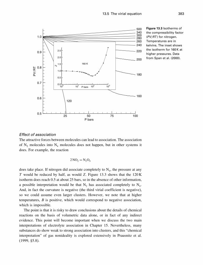
13.5 The virial equation 383
P bars
PV
/RT
25 50 75 1000.5
0.6
0.7
0.8
0.9
1.0
120
160
180
200
220
240260280300340500
P bars
Z
100 101 102 1030.0
0.5
1.0
1.5
2.0
2.5
160 K
Figure 13.3 Isotherms ofthe compressibility factor(P V/RT ) for nitrogen.Temperatures are inkelvins. The inset showsthe isotherm for 160 K athigher pressures. Datafrom Span et al. (2000).
Effect of associationThe attractive forces between molecules can lead to association. The associationof N2 molecules into N4 molecules does not happen, but in other systems itdoes. For example, the reaction
2NO2 = N2O4
does take place. If nitrogen did associate completely to N4, the pressure at anyT would be reduced by half, as would Z. Figure 13.3 shows that the 120Kisotherm does reach 0.5 at about 25 bars, so in the absence of other information,a possible interpretation would be that N2 has associated completely to N4.And, in fact the curvature is negative (the third virial coefficient is negative),so we could assume even larger clusters. However, we note that at highertemperatures, B is positive, which would correspond to negative association,which is impossible.
The point is that it is risky to draw conclusions about the details of chemicalreactions on the basis of volumetric data alone, or in fact of any indirectevidence. This point will become important when we discuss the two maininterpretations of electrolyte association in Chapter 15. Nevertheless, manysubstances do show weak to strong association into clusters, and this “chemicalinterpretation” of gas nonideality is explored extensively in Prausnitz et al.(1999, §5.8).
384 Equations of state
13.6 Thermal equations of state
As already mentioned, thermal EoS are those capable of directly producing val-ues of all thermodynamic properties, including heat capacity, entropy, enthalpy,and so on. They are based either on a formulation in terms of the Gibbs energy,if the independent variables are T and P, or in terms of the Helmholtz energyif the independent variables are T and V (or �). Over much of P–T space,either formulation is quite satisfactory, but when the two-phase vapor–liquidregion is involved, the Helmholtz energy (A) is invariably chosen, because fora given T and P, A has two different values for the vapor and liquid states, andso is capable of reporting different values for all parameters for these states.Gibbs energy, on the other hand, has the same value for the coexisting vaporand liquid, and so an equation for G cannot provide thermodynamic values foreach of the coexisting phases.
The development of these all-encompassing EoS has become a very largeand complex subject, which is more mathematical than thermodynamic. Fora recent summary, see Span (2000). It is not unusual for these equations,or rather sets of equations, to have more than 50 adjustable parameters, andeven the form of the equations is now adjustable by computer routines. Theequations are far too complex to present in detail here, and even programmingthem from the literature is a nontrivial task. Fortunately many are available inexecutable form.
We will discuss just a few of these, which are useful to Earth scientists.Thermal EoS have been developed only for pure substances and some binarysystems. For more complex systems some form of cubic or virial equation isnormally used.
13.6.1 Water substance
Water is generally thought of as a liquid, and the gaseous and solid formsget their own names, so for generality the term “water substance” is used toinclude all forms of H2O.
Water is arguably the most important compound on Earth, from many pointsof view. An equation of state for water was the goal for many researchersfor many years, and it proved to be a very difficult task, both experimentally(doing the experiments to obtain the data at high T and P) and theoretically(finding an equation to fit the data). Earth scientists have contributed their shareof attempts.
Burnham, Holloway, and DavisBurnham et al. (1969a) made extensive density measurements at high T andP, and published (1969b) tables of the important thermodynamic propertiesup to 1000 �C and 10 000 bars. As mentioned earlier, PVT measurementsalone cannot provide complete thermodynamic information, so these data were
13.6 Thermal equations of state 385
used to expand upward in pressure an earlier published formulation of thethermodynamic properties (Bain, 1964) which extended only to 1000 bars.No attempt was made to include values for ice or water vapor, and despitethe apparent simplicity of the isochore shapes (Figure 6.1) they were forcedto use three different sets of fit coefficients to cover different subregions ofthe whole T–P region. Many newer formulations have even more subregions.These data were later superseded, but are sufficiently accurate for most Earthscience applications, and are still used at times (e.g., Aranovitch and Newton,1996, 1997).
Helgeson and KirkhamHelgeson and Kirkham (1974a) reworked all the data available at that time, andinclude extensive references to earlier work. They used the data of Burnhamet al. as well as other data, and produced equations for many thermodynamicproperties not considered by Burnham et al., including the dielectric constant.They covered the region up to 900 �C and 10 kbar.
IAPWS formulationsThe International Association for the Properties of Water and Steam (IAPWS;up to 1989 just IAPS) has for many years sponsored the development ofincreasingly accurate equations of state for water.
Haar, Gallagher and KellThe formulation by Haar, Gallagher and Kell in 1984 (IAPS-84) was a majorstep forward in completeness and accuracy, and is incorporated into programsupcrt92. It is sufficiently accurate for all routine geochemical work, but hasnow been superseded by IAPWS-95.
Wagner and PrußThe latest IAPWS formulation is IAPWS-95, and is described by Wagner andPruß (2002).2 Software implementing this formulation is available from theNational Institute of Standards and Technology (NIST) in the form of programsteam, written by Harvey, Peskin and Klein (2000). A paper by Hill (1990)contains graphical comparisons of several previous equations of state.
Using the Wagner and Pruß notation, the basic equation has the form
f���T�= f ����T�+f r���T� (13.40)
where the Helmholtz energy f uses � instead of V , and is split into an ideal gaspart (f �) and a residual part (f r). This practice is common in the developmentof equations of state (§13.2.3). The Helmholtz energy is then transformed into
2 Information on the IAPWS formulations is available at www.iapws.org.
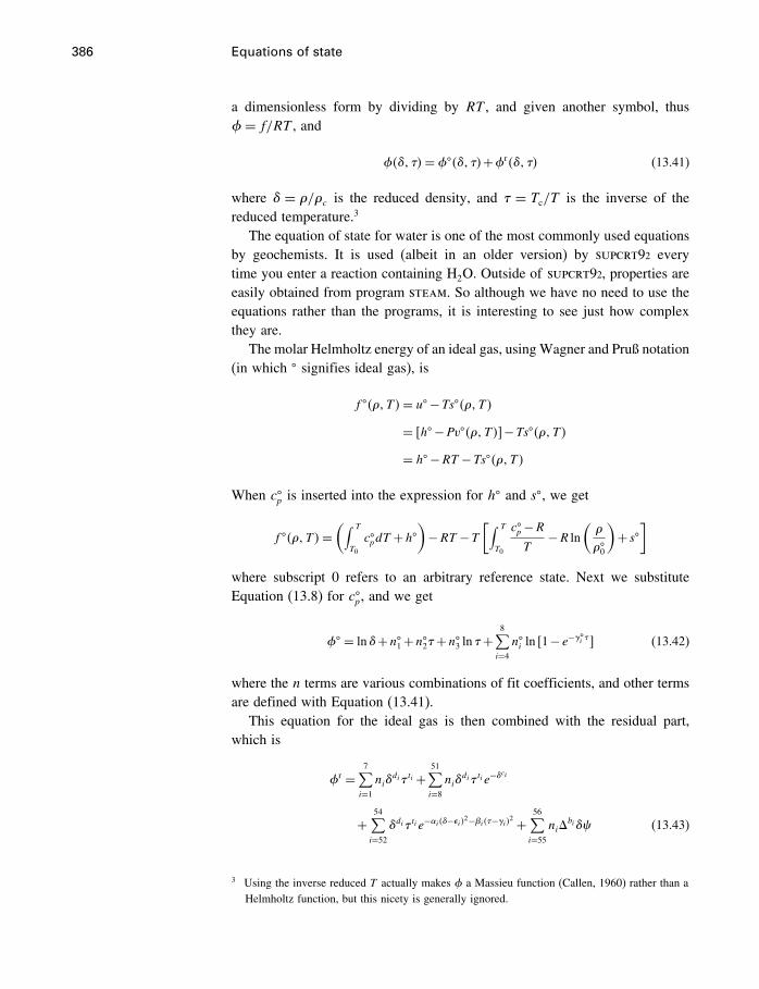
386 Equations of state
a dimensionless form by dividing by RT , and given another symbol, thus�= f/RT , and
���� ��= ����� ��+�r��� �� (13.41)
where � = �/�c is the reduced density, and � = Tc/T is the inverse of thereduced temperature.3
The equation of state for water is one of the most commonly used equationsby geochemists. It is used (albeit in an older version) by supcrt92 everytime you enter a reaction containing H2O. Outside of supcrt92, properties areeasily obtained from program steam. So although we have no need to use theequations rather than the programs, it is interesting to see just how complexthey are.
The molar Helmholtz energy of an ideal gas, usingWagner and Pruß notation(in which � signifies ideal gas), is
f ����T�= u� −Ts����T�= �h� −Pv����T��−Ts����T�= h� −RT −Ts����T�
When c�p is inserted into the expression for h� and s�, we get
f ����T�=(∫ T
T0
c�pdT +h�)−RT −T
[∫ T
T0
c�p −RT
−R ln(�
��0
)+ s�
]where subscript 0 refers to an arbitrary reference state. Next we substituteEquation (13.8) for c�p, and we get
�� = ln�+n�1+n�2�+n�3 ln �+8∑i=4
n�i ln �1− e−�i � � (13.42)
where the n terms are various combinations of fit coefficients, and other termsare defined with Equation (13.41).
This equation for the ideal gas is then combined with the residual part,which is
�r =7∑i=1
ni�di �ti +
51∑i=8
ni�di �ti e−�
ci
+54∑i=52
�di�ti e−i��−�i�2−�i��−i�2 +
56∑i=55
ni�bi�� (13.43)
3 Using the inverse reduced T actually makes � a Massieu function (Callen, 1960) rather than aHelmholtz function, but this nicety is generally ignored.
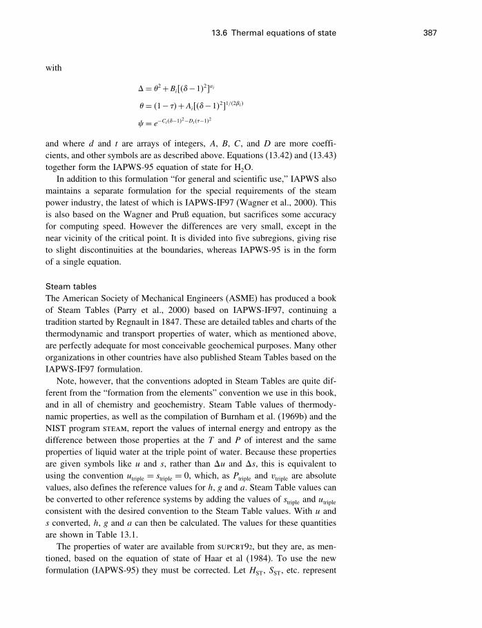
13.6 Thermal equations of state 387
with
�= �2+Bi���−1�2�ai
� = �1− ��+Ai���−1�2�1/�2�i�
� = e−Ci��−1�2−Di��−1�2
and where d and t are arrays of integers, A, B, C, and D are more coeffi-cients, and other symbols are as described above. Equations (13.42) and (13.43)together form the IAPWS-95 equation of state for H2O.
In addition to this formulation “for general and scientific use,” IAPWS alsomaintains a separate formulation for the special requirements of the steampower industry, the latest of which is IAPWS-IF97 (Wagner et al., 2000). Thisis also based on the Wagner and Pruß equation, but sacrifices some accuracyfor computing speed. However the differences are very small, except in thenear vicinity of the critical point. It is divided into five subregions, giving riseto slight discontinuities at the boundaries, whereas IAPWS-95 is in the formof a single equation.
Steam tablesThe American Society of Mechanical Engineers (ASME) has produced a bookof Steam Tables (Parry et al., 2000) based on IAPWS-IF97, continuing atradition started by Regnault in 1847. These are detailed tables and charts of thethermodynamic and transport properties of water, which as mentioned above,are perfectly adequate for most conceivable geochemical purposes. Many otherorganizations in other countries have also published Steam Tables based on theIAPWS-IF97 formulation.
Note, however, that the conventions adopted in Steam Tables are quite dif-ferent from the “formation from the elements” convention we use in this book,and in all of chemistry and geochemistry. Steam Table values of thermody-namic properties, as well as the compilation of Burnham et al. (1969b) and theNIST program steam, report the values of internal energy and entropy as thedifference between those properties at the T and P of interest and the sameproperties of liquid water at the triple point of water. Because these propertiesare given symbols like u and s, rather than �u and �s, this is equivalent tousing the convention utriple = striple = 0, which, as Ptriple and vtriple are absolutevalues, also defines the reference values for h, g and a. Steam Table values canbe converted to other reference systems by adding the values of striple and utripleconsistent with the desired convention to the Steam Table values. With u ands converted, h, g and a can then be calculated. The values for these quantitiesare shown in Table 13.1.
The properties of water are available from supcrt92, but they are, as men-tioned, based on the equation of state of Haar et al (1984). To use the newformulation (IAPWS-95) they must be corrected. Let HST, SST, etc. represent
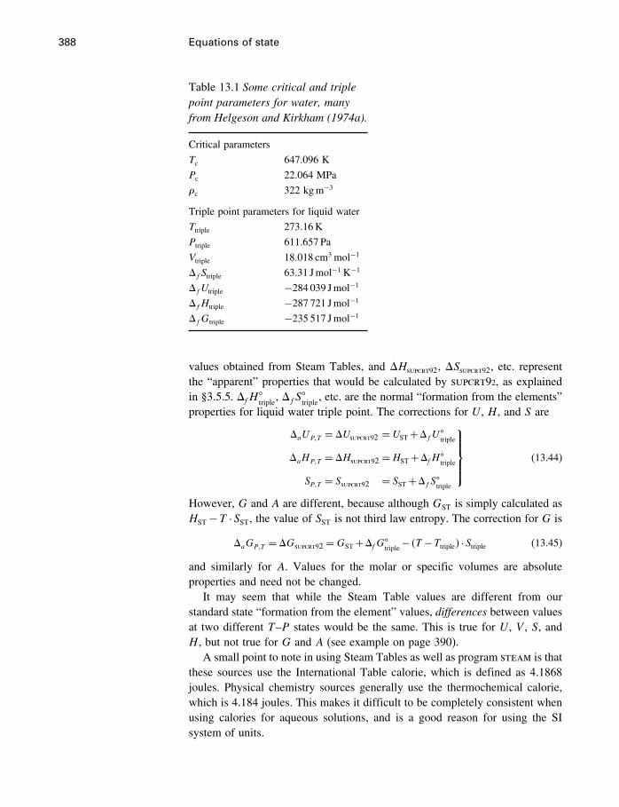
388 Equations of state
Table 13.1 Some critical and triplepoint parameters for water, manyfrom Helgeson and Kirkham (1974a).
Critical parameters
Tc 647.096 K
Pc 22.064 MPa
�c 322 kgm−3
Triple point parameters for liquid water
Ttriple 273.16K
Ptriple 611.657 Pa
Vtriple 18.018 cm3 mol−1
�fStriple 63.31 Jmol−1 K−1
�fUtriple −284 039 Jmol−1
�fHtriple −287 721 Jmol−1
�fGtriple −235 517 Jmol−1
values obtained from Steam Tables, and �Hsupcrt92, �Ssupcrt92, etc. representthe “apparent” properties that would be calculated by supcrt92, as explainedin §3.5.5. �fH
�triple
, �fS�triple
, etc. are the normal “formation from the elements”properties for liquid water triple point. The corrections for U , H , and S are
�aUP�T = �Usupcrt92 = UST+�fU �triple
�aHP�T = �Hsupcrt92 =HST+�fH�triple
SP�T = Ssupcrt92 = SST+�fS�triple
⎫⎪⎪⎪⎬⎪⎪⎪⎭ (13.44)
However, G and A are different, because although GST is simply calculated asHST−T ·SST, the value of SST is not third law entropy. The correction for G is
�aGP�T = �Gsupcrt92 =GST+�fG�triple
− �T −Ttriple� ·Striple (13.45)
and similarly for A. Values for the molar or specific volumes are absoluteproperties and need not be changed.
It may seem that while the Steam Table values are different from ourstandard state “formation from the element” values, differences between valuesat two different T–P states would be the same. This is true for U , V , S, andH , but not true for G and A (see example on page 390).
A small point to note in using Steam Tables as well as program steam is thatthese sources use the International Table calorie, which is defined as 4.1868joules. Physical chemistry sources generally use the thermochemical calorie,which is 4.184 joules. This makes it difficult to be completely consistent whenusing calories for aqueous solutions, and is a good reason for using the SIsystem of units.
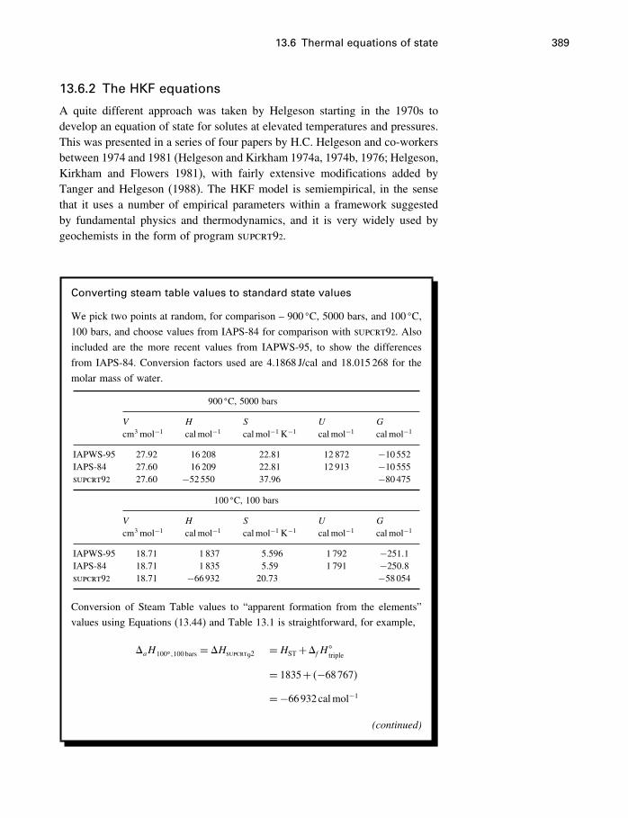
13.6 Thermal equations of state 389
13.6.2 The HKF equations
A quite different approach was taken by Helgeson starting in the 1970s todevelop an equation of state for solutes at elevated temperatures and pressures.This was presented in a series of four papers by H.C. Helgeson and co-workersbetween 1974 and 1981 (Helgeson and Kirkham 1974a, 1974b, 1976; Helgeson,Kirkham and Flowers 1981), with fairly extensive modifications added byTanger and Helgeson (1988). The HKF model is semiempirical, in the sensethat it uses a number of empirical parameters within a framework suggestedby fundamental physics and thermodynamics, and it is very widely used bygeochemists in the form of program supcrt92.
Converting steam table values to standard state values
We pick two points at random, for comparison – 900 �C, 5000 bars, and 100 �C,100 bars, and choose values from IAPS-84 for comparison with supcrt92. Also
included are the more recent values from IAPWS-95, to show the differences
from IAPS-84. Conversion factors used are 4.1868 J/cal and 18.015 268 for the
molar mass of water.
900 �C, 5000 bars
V H S U G
cm3 mol−1 calmol−1 calmol−1 K−1 calmol−1 calmol−1
IAPWS-95 27.92 16 208 22.81 12 872 −10552IAPS-84 27.60 16 209 22.81 12 913 −10555supcrt92 27.60 −52550 37.96 −80475
100 �C, 100 bars
V H S U G
cm3 mol−1 calmol−1 calmol−1 K−1 calmol−1 calmol−1
IAPWS-95 18.71 1 837 5.596 1 792 −251�1IAPS-84 18.71 1 835 5.59 1 791 −250�8supcrt92 18.71 −66932 20.73 −58054
Conversion of Steam Table values to “apparent formation from the elements”
values using Equations (13.44) and Table 13.1 is straightforward, for example,
�aH100��100bars = �Hsupcrt92=HST+�fH
�triple
= 1835+ �−68767�
=−66932 calmol−1
(continued)
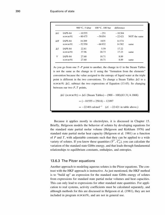
390 Equations of state
900 �C, 5 kbar 100 �C, 100 bar difference
�G IAPS-84 −10555 −251 −10304supcrt92 −80475 −58054 −22421 NOT the same
�H IAPS-84 16 209 1835 14 374supcrt92 −52550 −66932 14 382 same
�S IAPS-84 22.81 5.59 17.22supcrt92 37.96 20.73 17.23 same
V IAPS-84 27.60 18.71 8.89supcrt92 27.60 18.71 8.89 same
As you go from one T–P point to another, the change in G in the Steam Tables
is not the same as the change in G using the “formation from the elements”
convention because the value assigned to the entropy of liquid water at the triple
point is different in the two conventions. To change a Steam Tables �G to a
supcrt92 �G, subtract the two expressions of Equation (13.45). So changing
between our two P�T points,
�G �supcrt92�= �G (Steam Tables)− �900−100��63�31/4�1868�
= �−10555+250�8�−12097
=−22401calmol−1 (cf. −22421 in table above.)
Because it applies mostly to electrolytes, it is discussed in Chapter 15.Briefly, Helgeson models the behavior of solutes by developing equations forthe standard state partial molar volume (Helgeson and Kirkham 1976) andstandard state partial molar heat capacity (Helgeson et al. 1981) as a functionof P and T , with adjustable constants such that they can be applied to a widevariety of solutes. If you know these quantities (V
�, C
�P), you can calculate the
variation of the standard state Gibbs energy, and that leads through fundamentalrelationships to equilibrium constants, enthalpies, and entropies.
13.6.3 The Pitzer equations
Another approach to modeling aqueous solutes is the Pitzer equations. The con-trast with the HKF approach is instructive. As just mentioned, the HKF methodis to “build up” an expression for the standard state Gibbs energy of solutesfrom expressions for standard state partial molar volumes and heat capacities.This can only lead to expressions for other standard state quantities. For appli-cation to real systems, activity coefficients must be calculated separately, andalthough methods for this are discussed in Helgeson et al. (1981), they are notincluded in program supcrt92, and are not in general use.
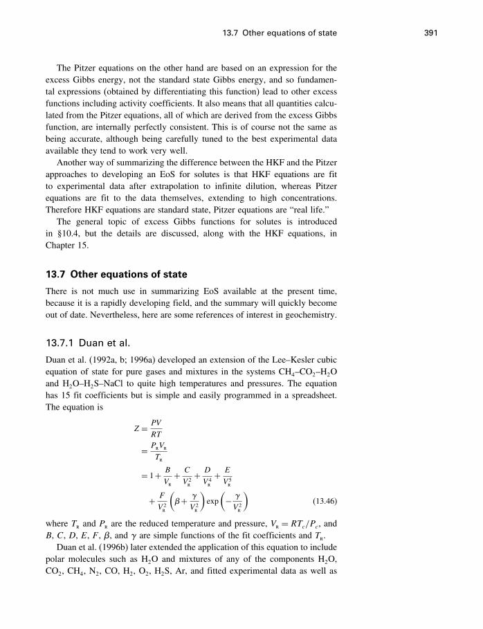
13.7 Other equations of state 391
The Pitzer equations on the other hand are based on an expression for theexcess Gibbs energy, not the standard state Gibbs energy, and so fundamen-tal expressions (obtained by differentiating this function) lead to other excessfunctions including activity coefficients. It also means that all quantities calcu-lated from the Pitzer equations, all of which are derived from the excess Gibbsfunction, are internally perfectly consistent. This is of course not the same asbeing accurate, although being carefully tuned to the best experimental dataavailable they tend to work very well.
Another way of summarizing the difference between the HKF and the Pitzerapproaches to developing an EoS for solutes is that HKF equations are fitto experimental data after extrapolation to infinite dilution, whereas Pitzerequations are fit to the data themselves, extending to high concentrations.Therefore HKF equations are standard state, Pitzer equations are “real life.”
The general topic of excess Gibbs functions for solutes is introducedin §10.4, but the details are discussed, along with the HKF equations, inChapter 15.
13.7 Other equations of state
There is not much use in summarizing EoS available at the present time,because it is a rapidly developing field, and the summary will quickly becomeout of date. Nevertheless, here are some references of interest in geochemistry.
13.7.1 Duan et al.
Duan et al. (1992a, b; 1996a) developed an extension of the Lee–Kesler cubicequation of state for pure gases and mixtures in the systems CH4–CO2–H2Oand H2O–H2S–NaCl to quite high temperatures and pressures. The equationhas 15 fit coefficients but is simple and easily programmed in a spreadsheet.The equation is
Z = PV
RT
= PrVrTr
= 1+ B
Vr+ C
V 2r
+ D
V 4r
+ E
V 5r
+ F
V 2r
(�+
V 2r
)exp(−
V 2r
)(13.46)
where Tr and Pr are the reduced temperature and pressure, Vr = RTc/Pc, andB, C, D, E, F , �, and are simple functions of the fit coefficients and Tr.
Duan et al. (1996b) later extended the application of this equation to includepolar molecules such as H2O and mixtures of any of the components H2O,CO2, CH4, N2, CO, H2, O2, H2S, Ar, and fitted experimental data as well as
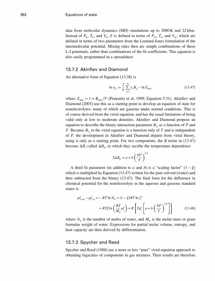
392 Equations of state
data from molecular dynamics (MD) simulations up to 2000K and 22 kbar.Instead of Pr, Tr, and Vr, Z is defined in terms of Pm, Tm and Vm, which aredefined in terms of two parameters from the Lennard-Jones formulation of theintermolecular potential. Mixing rules then are simple combinations of theseL-J potentials, rather than combinations of the fit coefficients. This equation isalso easily programmed in a spreadsheet.
13.7.2 Akinfiev and Diamond
An alternative form of Equation (13.38) is
lnfi =2V
m∑j=1
xjBij− lnZmix (13.47)
where Zmix = 1+Bmix/V (Prausnitz et al. 1999, Equation 5.31). Akinfiev andDiamond (2003) use this as a starting point to develop an equation of state fornonelectrolytes, many of which are gaseous under normal conditions. This isof course derived from the virial equation, and has the usual limitation of beingvalid only at low to moderate densities. Akinfiev and Diamond propose anequation to describe the binary interaction parameter Bij as a function of P andT . Because Bij in the virial equation is a function only of T and is independentof P, the development in Akinfiev and Diamond departs from virial theory,using it only as a starting point. For two components, the B terms in (13.47)become �B, called �B�, to which they ascribe the temperature dependence
2�B� = a+b(103
T
)0�5
A third fit parameter (in addition to a and b) is a “scaling factor” �1− ��which is multiplied by Equation (13.47) written for the pure solvent (water) andthen subtracted from the binary (13.47). The final form for the difference inchemical potential for the nonelectrolyte in the aqueous and gaseous standardstates is
��2�aq−��
2�g =−RT lnNw+ �1−��RT ln f �i
+RT� ln(RT
Mw��i
)+R
{T��i
[a+b
(103
T
)0�5]}
(13.48)
where Nw is the number of moles of water, and Mw is the molar mass or gramformulas weight of water. Expressions for partial molar volume, entropy, andheat capacity are then derived by differentiation.
13.7.3 Spycher and Reed
Spycher and Reed (1988) use a more or less “pure” virial equation approach toobtaining fugacities of components in gas mixtures. Their results are therefore
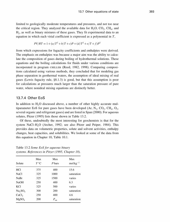
13.7 Other equations of state 393
limited to geologically moderate temperatures and pressures, and not too nearthe critical region. They analyzed the available data for H2O, CO2, CH4, andH2, as well as binary mixtures of these gases. They fit experimental data to anequation in which each virial coefficient is expressed as a polynomial in T ,
PV/RT = 1+ �a/T 2+b/T + c�P+ �d/T 2+ e/T +f�P2
from which expressions for fugacity coefficients and enthalpies were derived.The emphasis on enthalpies was because a major aim was the ability to calcu-late the composition of gases during boiling of hydrothermal solutions. Theseequations and the boiling calculations for fluids under various conditions areincorporated in program chiller (Reed, 1982, 1998). Comparing composi-tions calculated using various methods, they concluded that for modeling gasphase separation in geothermal waters, the assumption of ideal mixing of realgases (Lewis fugacity rule, §8.1.3) is good, but that this assumption is poorfor calculations at pressures much larger than the saturation pressure of purewater, where nonideal mixing equations are distinctly better.
13.7.4 Other EoS
In addition to H2O discussed above, a number of other highly accurate mul-tiparameter EoS for pure gases have been developed (Ar, N2, CO2, CH4, O2,several organic and refrigerant gases) and are listed in Span (2000). For aqueoussolutes, Pitzer (1995) lists those shown in Table 13.2.
Of these, undoubtedly the most interesting for geochemists is that for thesystem NaCl–H2O (Archer, 1992; see also Pitzer and Peiper, 1984). Thisprovides data on volumetric properties, solute and solvent activities, enthalpychanges, heat capacities, and solubilities. We looked at some of the data fromthis equation in Chapter 10, Table 10.1.
Table 13.2 Some EoS for aqueous binarysystems. References in Pitzer (1995, Chapter 18).
Max Max Max
Solute T �C P bars mol kg−1
HCl 375 400 15.6
NaCl 325 1000 saturation
NaBr 325 1500 varies
NaOH 250 400 6.3
KCl 325 500 varies
Na2SO4 300 200 saturation
CaCl2 250 400 4.6
MgSO4 200 Psat saturation
394 Equations of state
13.8 Summary
Good equations of state are valuable things, because they supply you withneeded thermodynamic information, not only more easily than doing experi-ments or even just looking up numbers in tables, but some kind of averagednumbers from carefully selected data sets. There are two main approaches todeveloping equations of state (there may be more, but we are keeping thingssimple here).
One is the many variations of the cubic equation relating P, V , and T , whichis very good at predicting vapor–liquid equilibria, but for which no formulationhas yet been found to work with all pertinent systems. And although in principlecubic equations can work with any number of components in a mixture, the“mixing rules” are another source of more or less empirical guesswork.
The other main approach is to develop an equation which returns a valueof G as a function of system T and P, or A as a function of system T andV . These equations have reached a very high state of development, having 50or more fit coefficients and a mathematical form which is also a subject ofcomputer fitting procedures. The EoS for water is an outstanding example ofthis approach. However, the extension of this approach to handle mixtures isa formidable research task. Span (2000) is a good introduction to this subject,and includes many specialized EoS not mentioned here.
When it comes to high temperature and pressures involving aqueous elec-trolytes, geochemists have little choice at the present time but to use the HKFmodel in the form of program supcrt92, although alternative approaches arebeing explored. The Pitzer equations are another possibility, but so far aremostly restricted to near ambient conditions. They do, however, perform muchbetter than HKF at high concentrations.
14Solid solutions
14.1 Introduction
Let’s say you are mapping a field area consisting of metamorphic rocks. Oneunit contains garnet, plagioclase, kyanite, and quartz, with a few other phases.Having studied mineralogy, you know that garnet and plagioclase are not“pure” phases, made up of a single component but are solid solutions of several“end-member” components.1 You also know that these minerals are related bythe “anorthite breakdown reaction,” written
3CaAl2Si2Oplag8 = Ca3Al2Si3O
garnet12 +2Al2SiO
kyanite5 +SiOqtz
2 (14.1)
for which the equilibrium constant is
K = aCa3Al2Si3O12a2Al2SiO5
aSiO2
a3CaAl2Si2O8
(14.2)
You analyze your minerals, and the results are reported in terms of oxides.A typical garnet analysis would look like Table 14.1. To make any thermody-namic use of this reaction, you evidently need to somehow extract an activityof Ca3Al2Si3O12 from this information, as well as the activity of CaAl2Si2O8
from a similar analysis of the plagioclase. You know that quartz and kyanite aregenerally quite pure, so that assuming aSiO2
= 1 and aAl2SiO5= 1 will probably
be close enough.How do you do this? And why would it be useful? A complete answer
would take a whole book, and is more appropriate to a course in metamorphicpetrology, but we can fairly easily see how thermodynamics is applied in suchcases. Newton and Haselton (1981) give a summary of the thermodynamics ofthis reaction, as well as its use as a geobarometer, that is, a mineral assemblagethat, when analyzed thermodynamically, will give an estimate of the pressureat the time the minerals equilibrated.
1 Recall that we introduced the concept of components in Chapter 2. Many discussions use theterm rather loosely, referring to compositional terms generally. In other cases, such as here,we use the term strictly, as the smallest number of formulas needed to express a systemcomposition (Chapter 11).
395
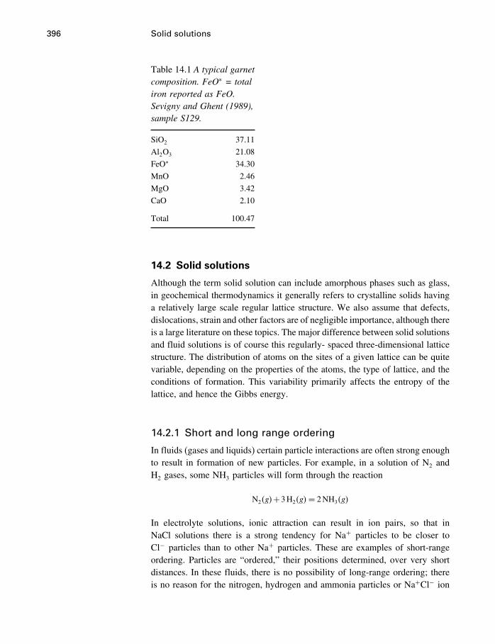
396 Solid solutions
Table 14.1 A typical garnetcomposition. FeO∗ = totaliron reported as FeO.Sevigny and Ghent (1989),sample S129.
SiO2 37.11
Al2O3 21.08
FeO∗ 34.30
MnO 2.46
MgO 3.42
CaO 2.10
Total 100.47
14.2 Solid solutions
Although the term solid solution can include amorphous phases such as glass,in geochemical thermodynamics it generally refers to crystalline solids havinga relatively large scale regular lattice structure. We also assume that defects,dislocations, strain and other factors are of negligible importance, although thereis a large literature on these topics. The major difference between solid solutionsand fluid solutions is of course this regularly- spaced three-dimensional latticestructure. The distribution of atoms on the sites of a given lattice can be quitevariable, depending on the properties of the atoms, the type of lattice, and theconditions of formation. This variability primarily affects the entropy of thelattice, and hence the Gibbs energy.
14.2.1 Short and long range ordering
In fluids (gases and liquids) certain particle interactions are often strong enoughto result in formation of new particles. For example, in a solution of N2 andH2 gases, some NH3 particles will form through the reaction
N2�g�+3H2�g�= 2NH3�g�
In electrolyte solutions, ionic attraction can result in ion pairs, so that inNaCl solutions there is a strong tendency for Na+ particles to be closer toCl− particles than to other Na+ particles. These are examples of short-rangeordering. Particles are “ordered,” their positions determined, over very shortdistances. In these fluids, there is no possibility of long-range ordering; thereis no reason for the nitrogen, hydrogen and ammonia particles or Na+Cl− ion
14.2 Solid solutions 397
pairs to be regularly distributed with respect to each other – they mix randomlyat high speeds.2
Crystalline solids, however, can have long-range as well as short-rangeordering. For example, in disordered Cu3Au, the gold atoms are arrayed ran-domly at sites normally occupied by copper atoms in the copper lattice, butgiven proper heat treatment, all of the gold atoms become located at cubecorners and copper atoms at face-centered positions of the unit-cell cube. TheAu atoms then show long range order. Silicates are basically an ordered arrange-ment of oxygen atoms with interstices of various sizes and shapes, dependingon the arrangement of the oxygens. Cations will then show preferences forsome interstitial sites rather than others. For example, a particular cation maybe too big for some sites, and the sites it fits into may be regularly spaced,resulting in long range order for that cation.
If there is a tendency for certain pairs of cations to prefer to be on nearbysites, perhaps to preserve a local charge balance, the result is a short rangeordering. This tendency can be weak or strong, analogous to weak or strongcomplex formation. If the tendency is very strong, the cation pair can beconsidered to be a particle or molecule, and the distribution of particles overavailable sites can be calculated using this molecule rather than the individualatoms. Carried to its logical extreme results in “molecular mixing,” in whichcomplete mineral formulas are considered to be the mixing units. This isnot usually the best approach. Unfortunately, it is difficult to determine theextent of short range ordering in crystals, and taking it into account greatlycomplicates the thermodynamic treatment. One such approach is the “quasi-chemical” method of Guggenheim (1952). If you need to know more about this,an introduction and applications are given by Saxena (1973). The most commonapproach, however, is to ignore short range order, and to calculate the molefractions of solid solution components by considering the distribution of ionson crystallographic sites, a process called mixing-on-sites, or “site-mixing.”
The rest of this chapter is in two parts. First, we consider how to calculatemole fractions in solid solutions assumed to have only long range order, andhow to combine these mole fractions into Raoultian activities. Then we considerthe determination of activity coefficients in (binary) solid solutions, and howregular solution and Margules equations are used to systematize these.
14.2.2 Mixing on sites
Thermodynamic mole fractionsWe know that for Raoultian ideal solutions, ai = xi, or activity is equal tomole fraction, so to calculate the Raoultian activity of solid solution compo-nents, all we have to do is calculate their mole fractions. If there is only one
2 Theories having partial long range ordering in electrolyte solutions have been proposed, e.g.,Pytkowicz et al. (1977).
398 Solid solutions
crystallographic site on which elements mix randomly, there is no difficulty.An example is the alkali feldspar solid solution, in which Na and K mix ran-domly on one crystallographic site. The mole fractions of Na and K on thissite, are then quite evidently the same as the mole fractions of NaAlSi3O8 andKAlSi3O8, because there are no other changes. That is,
xAb =mNaAlSi3O8
mNaAlSi3O8+mKAlSi3O8
= mNa
mNa +mK
So if you wanted the activity of the albite component in this solid solution,and you didn’t mind assuming it was an ideal solution, all you need to do isanalyze the feldspar for Na and K.
If there is more than one site on which mixing takes place, the thermo-dynamics remains simple, but determining the mole fractions becomes moredifficult. Equation (7.20),
�mixGideal sol’n = RT∑i
xi ln xi [7.20]
gives us the Gibbs energy of mixing on one site. If there are several siteson which mixing is taking place, it gives the energy change on each oneseparately. To combine these terms to obtain the total molar energy term forthe system, we need to know how many of each site there are, which isgiven by the chemical formulas of the crystal. For example, garnet has theformulas X3Y2Si3O12, where the X sites are cubic (8-coordinated), the Y sitesare octahedral (6-coordinated), and the Si site is tetrahedral (4-coordinated). Ifthe X sites contain randomly mixed Mg2+, Ca2+, Mn2+, and Fe2+, and the Ysites contain randomly mixed Al3+ and Fe3+, there are several possible mineral“end-member” species, such as
pyrope Mg3Al2Si3O12
grossular Ca3Al2Si3O12
almandine Fe2+3 Al2Si3O12
spessartine Mn3Al2Si3O12
khoharite Mg3Fe3+2 Si3O12
andradite Ca3Fe3+2 Si3O12
To simplify, let’s consider that Mn2+ and Fe2+ in the X site have lowconcentrations and are insignificant, so that the garnet is essentially �Mg�Ca�3�Al�Fe�2Si3O12. Including the other elements adds no difficulty, it just addsmore terms of the same type, and makes the equations longer.
Now we have four elements mixing on two sites. This looks like a case offour components, pyrope, grossular, andradite and khoharite. However, any ofthese four formulas can be written as a linear combination of the other three(Spear, 1995, p. 184). We can therefore describe all compositions of this garnet
14.2 Solid solutions 399
in terms of any three of these four components, and we choose to use pyrope,grossular, and andradite.
The total Gibbs energy of mixing can then be written in two different butequivalent ways. We can use Equation (7.20) with end-member components,or with ionic mixing on individual sites. Using our three components, we have
�mixGideal sol’n = RT�xMg3Al2Si3O12ln xMg3Al2Si3O12
+xCa3Al2Si3O12ln xCa3Al2Si3O12
+xCa3Fe2Si3O12ln xCa3Fe2Si3O12
�
= RT�xpyrope ln xpyrope+xgrossular ln xgrossular +xandradite ln xandradite� (14.3)
This applies to ideal mixing. If each log term is corrected with an appropriateactivity coefficient, we get
�mixG= RT�xpyrope lnapyrope+xgrossular lnagrossular +xandradite lnaandradite� (14.4)
Considering mixing on individual sites, we can write
�mixGideal sol’n =−T �mixSideal sol’n
= 3RT�xMg ln xMg+xCa ln xCa�+2RT�xAl ln xAl+xFe3+ ln xFe3+�= RT�xMg ln x
3Mg+xCa ln x3Ca +xAl ln x2Al+xFe3+ ln x2Fe3+� (14.5)
where, for example,
xMg =nMg
nMg+nCain the normal fashion, and for which the general notation is
�mixGideal sol’n = RTk∑j=1
nj∑i
xi�j ln xi�j (14.6)
where k is the total number of nonequivalent sites (2 in this example), nj isthe number of times the constituent in question appears in the formulas for thejth site in the solution (in this example, nj = 2 for the X and Y sites), and xi�jis the mole fraction of the ith ion on the jth site (X, or Y site). We could havek= 3 by including mixing of Al and Si on the Si site. One thing to watch forin applying this equation is to make sure that a charge balance is maintained.In other words, the substitutions should be independent of one another. SeeUlbrich and Waldbaum (1976) for a detailed discussion of this topic.
This result is of limited usefulness. What we really want in most cases is notthe total mixing energy, but the activity of some component in a solid solutioncontaining that component. In our example, we want to know the activity ofthe grossular (Ca3Al2Si3O12) component, so as to be able to use our mineralcomposition in Equation (14.2). To get an expression for the activity of such
400 Solid solutions
components, we first transform (14.5) into a form containing the number ofmoles of our various components. Following Spear (1995, p. 185), we write amass balance for each cation,
nMg = 3xpyrope+0xgrossular +0xandradite
nCa = 0xpyrope+3xgrossular +3xandradite
nAl = 2xpyrope+2xgrossular +0xandradite
nFe = 0xpyrope+0xgrossular +2xandradite
or (using ⇒ to mean “defined as thermodynamic mole fraction”),
nMg/3= xpyrope ⇒ xMg
nCa/3 = xgrossular +xandradite ⇒ xCa
nAl/2 = xpyrope+xgrossular ⇒ xAl
nFe/2 = xandradite ⇒ xFe
giving the relationship between the number of moles of ions on sites andthe (thermodynamic) mole fractions (x) of our chosen mineral components.Substituting these relations into Equation (14.5) we get
�mixGideal sol’n = RT�xpyrope lnx3Mg+ �xgrossular +xandradite� lnx3
Ca
+ �xpyrope+xgrossular� lnx2Al+xandradite lnx2
Fe3+ �
and rearranging terms,
�mixGideal sol’n = RT�xpyrope ln�x3Mgx
2Al�+xgrossular ln�x3
Cax2Al�
+xandradite ln�x3Cax
2Fe�� (14.7)
Comparing this with Equation (14.4), we see that our component activity termsare
apyrope = x3Mgx
2Al
agrossular = x3Cax
2Al
aandradite = x3Cax
2Fe3+
⎫⎪⎪⎪⎬⎪⎪⎪⎭ (14.8)
where the thermodynamic mole fractions are calculated as shown. An examplewill help to clarify how this is done (page 402).
All this assumes that we have defined a mole of grossular as Ca3Al2Si3O12,and similarly for the other components. If we defined the mole of grossular asCaAl2/3SiO4, that is, based on four oxygens instead of 12, we would have
aCaAl2/3SiO4= xCax
2/3Al
14.2 Solid solutions 401
as explained in §9.10.2. If there is no substitution on the Al (octahedral) site,xAl = 1, xCa = xCa, and
aCaAl2/3SiO4= xCa
analogous to the alkali feldspars.
14.2.3 Complications
If that was all there was to determining activities in solid solutions, a largepart of metamorphic petrology would be a lot simpler than it is. But there area number of complicating factors.
• As already mentioned, we need activity coefficients as well as thermodynamic mole
fractions. We discuss this in the next section.• Ionic mixing may be complicated by the need for charge balance. For example in
plagioclase, Ca2+ cannot substitute for Na+ unless Al3+ substitutes for Si4+ as well.• Mixing can also be complicated by “Al avoidance.” Substitution of Al3+ for Si4+ on
tetrahedral sites may take place in such a way as to avoid having Al on adjacent sites,
minimizing distortion of the lattice structure.• It may happen that site-mixing results in a formulas that does not result in x = 1 for
the pure components. In these cases a “normalization factor” is used, to ensure that
end-member mole fractions are 1.0.
Activities from solid solution compositions
We start with the garnet analysis in Table 14.1. The idea is to calculate howmany cations of each type there are in the analysis, assuming there are a totalof 12 oxygens. Following the method of Powell (1978, p. 75), we recalculate asfollows:
oxide wt.% A B C D E
SiO2 37.11 0.6176 1.2353 0.6176 2.98 5.9534Al2O3 21.08 0.2067 0.6202 0.4135 1.99 2.9893FeO∗ 34.30 0.4774 0.4774 0.4774 2.30 2.3009MnO 2.46 0.0347 0.0347 0.0347 0.17 0.1671MgO 3.42 0.0848 0.0848 0.0848 0.41 0.4089CaO 2.10 0.0374 0.0374 0.0374 0.18 0.1805
Total 2.4899 12.000
F = 12/2�4899
(continued)
402 Solid solutions
where the columns are calculated as follows:column A is the weight % divided by the molecular weightcolumn B is A times the number of oxygens in the formulascolumn C is A times the number of cations in the formulascolumn D is C times F , and is the number of cations per 12 oxygenscolumn E is D times the ratio of oxygens to cations in the formulas, which is acheck on the arithmetic.
The garnet composition can then be expressed as
�Mg0�41Ca0�18Fe2�30Mn0�17�Al2Si3O12�
where the difference between 1.99 and 2 for Al and between 2.98 and 3 for Sican be considered as analytical uncertainty, or perhaps that some small amountof substitution has taken place.
The mole fractions on the cubic site are then
xFe = 2�30/�2�30+0�17+0�41+0�18�= 0�753
xMn = 0�17/�2�30+0�17+0�41+0�18�= 0�055
xMg = 0�41/�2�30+0�17+0�41+0�18�= 0�134
xCa = 0�18/�2�30+0�17+0�41+0�18�= 0�059
and the ideal solution activities are (where xAl = 1)
aalmandine = x3Fex2Al = 0�426
aspessartine = x3Mnx2Al = 0�00016
apyrope = x3Mgx2Al = 0�0024
agrossular = x3Cax2Al = 0�00021
See Powell (1978) for many other examples.
• It often happens that the two end-members of a solid solution series have different
crystallographic structures. These will have different energies and entropies, which
must be accounted for in calculating phase relations.
• Where independent mixing occurs on more than one site, as in the garnet case,
the number of independent components is less than the number of possible end-
member components. These are “reciprocal solid solutions,” and this gives rise to
the possibility of an additional energy term called “reciprocal Gibbs energy” which
must be included in the energy of mixing, and which therefore affects the activity
calculations (Wood and Nicholls, 1978).
14.3 Activity coefficients in solid solutions 403
• We have considered only the case where individual cations mix randomly only on
one site. However, rather than being random, they may show some variable degree of
“order–disorder,” such as the variable Al–Si mixing on the tetrahedral site in feldspars,
resulting in the “high” (e.g., sanidine) and “low” (e.g., maximummicrocline) varieties.
Other minerals exhibit “cross-site mixing,” in which an individual cation can mix
to a variable degree on two (or more) sites, also resulting in order–disorder. It also
results in such solutions being reciprocal solid solutions.• Implicitly assumed in the thermodynamic analysis of all experimental and natural
assemblages is the presence of local equilibrium (§2.3.2). In petrology, an additional
problem is knowing at what stage in the long, complex history of the rock the assumed
equilibrium was attained.
Most of these complications are considered in some detail by Spear (1995,Chapter 7).
14.3 Activity coefficients in solid solutions
In Chapter 5 we discussed how to get thermodynamic data, and we said themethods should be those based on measuring heat and work, such as calorime-try, and we assumed implicitly that we were dealing with pure substances. Nowwe are dealing with substances in solution, and the problem is to determine byhow much the properties of the pure substance (strictly speaking the substancein some known state) are changed by being in solution. When we know that,we can determine which way reactions involving dissolved substances willgo. We have derived a function, the activity, which tells us by how muchthe Gibbs energy changes in solution. Activities have a composition part andan activity coefficient part, and the hard part in determining the activity isgetting an activity coefficient, because we usually have the compositional part(although that can get a bit tricky in solid solutions, as we have just seen). Someasuring activity coefficients is fundamental to using solutions in chemicalreactions. Failing any knowledge of activity coefficients we can fall back ontwo alternatives:
• Assume that property changes are those that would occur if our solutions were ideal,
that is, we can assume activity coefficients are 1.0, or• Use some theoretical calculation or estimation of the activity coefficient.
Both these alternatives have drawbacks, but are very commonly used in theEarth sciences, where complex solutions at high temperatures and pressures arecommonly of interest. The problem is that determining activity coefficients isdifficult, and for the most part confined to binary and ternary systems. In solidsolutions, it can be done in various ways, such as
404 Solid solutions
• Comparing the composition of a phase in a buffered assemblage with the ideal
composition.
• Calorimetric measurements of enthalpies and entropies of solid solutions, combining
these into �mixG values, and comparing these with the ideal values.
• Equilibrating a solid solution with another phase in which the activity coefficients are
known, such as an (almost) ideal gas, a dilute solution, or a phase having previously
measured activity coefficients.
• Analyzing solvus data.
We will have a brief look at each of these methods. In the process, we willsee the pervasive use of regular solution and Margules equations.
14.3.1 Buffered assemblages
Hensen et al. (1975) experimentally equilibrated the assemblage garnet–anorthite–kyanite–quartz at temperatures of 1000–1300 �C, 15–21 kilobars,together with a source of Mg (enstatite, MgSiO3). Mg does not enter the anor-thite, kyanite, or quartz structures, only the garnet, and that to a variable extent,depending on the temperature and pressure. The assemblage anorthite–kyanite–quartz has three components (CaO, Al2O3, SiO2) and three phases, and so isa buffering assemblage at a given T and P (see §11.5). This means that theactivity of Ca3Al2Si3O12 is fixed at that T and P. It is also equal to the equilib-rium constant for the anorthite breakdown reaction, Equation (14.2), becauseall the other activity terms are fixed at 1.0. That is,
K = aCa3Al2Si3O12a2Al2SiO5
aSiO2
a3CaAl2Si2O8
= aCa3Al2Si3O12when aAl2SiO5
� aSiO2� and aCaAl2Si2O8
= 1�0 (14.9)
which is actually just another way of showing that aCa3Al2Si3O12is a constant
at T, P. Therefore a knowledge of how the equilibrium constant changes withpressure will allow a calculation of the grossular activity.
Adding Mg to the garnet has the effect of enlarging the garnet stability field,for the same reason that adding salt to water lowers the freezing point. Thiseffect is discussed in Chapter 17 and illustrated in Figure 17.13. In the presentcase the reaction is not between a solid and a liquid, but between two solidassemblages, but the principle is exactly the same – adding a component lowersthe Gibbs energy and the phase field expands as a result. Figure 14.1 showsthe equilibrium curve for this reaction calculated by supcrt92 based on severalsets of experimental data detailed in Helgeson et al. (1978). Also shown arethe experimental points of Hensen et al. (1975) at lower pressures, in whichthe garnet is not pure grossular, but a grossular–pyrope solid solution.
14.3 Activity coefficients in solid solutions 405
Temperature, °C
Pre
ssur
e, k
bar
800 1000 1200 1400 160014
16
18
20
22
24
26
28
30
32
34
36
Anorthite
Grossular
+Kyanite
+Quartz
Effect of adding Mg to Grossularite
Pure phase equilib
rium
Hensen et al. (1975) experimental points
Figure 14.1 The univariant equilibrium curve for the anorthite breakdown reaction,3 anorthite = grosssular + 2 kyanite + quartz. Calculated with the univariant curveoption in supcrt92. The effect of adding Mg to the grossular is to lower theequilibrium pressure, as shown by the data of Hensen et al. (1975).
After equilibrating the phases at T and P, the garnet is analyzed, and theideal Raoultian activity of Ca3Al2Si3O12 is calculated from the thermodynamicmole reaction as in Equations (14.8), i.e.,
aidealgrossular = xgrossular
= x3Cax
2Al
except that in this case there is only Ca–Mg substitution, so xAl = 1, andxgrossular = x3Ca. The activity coefficient is then calculated from
Ca3Al2Si3O12= agrossular
xgrossular
The details of this calculation are shown on page 407.This study has been included partly because it illustrates the usefulness of
the buffering concept, which is the basis of the method. The actual value ofthe interaction coefficients in garnets are still a subject of some debate, asdiscussed by Newton and Haselton (1981).
14.3.2 Calorimetric measurements
The enthalpies of solution of several synthetic pyrope–grossular garnets weredetermined by Newton et al. (1977) by dissolving them in a liquid (2PbO ·
406 Solid solutions
Calculation of grossular activity and activity coefficient
In §9.8 we discussed the effect of pressure on an equilibrium constant, in the
special case in which the �rV� can be considered constant. This equation is
lnKP = lnKP=1−�rV
�
RT�P−1� [9.36]
but in that case we assumed that the standard state pressure was 1 bar. The
equation can of course be used to calculate the change in lnK between any two
pressures, as long as �rV� remains constant. In this case, we need the change
in lnK between the pressure of the pure grossular equilibrium curve (call it
P�) and the pressure of the grossular–pyrope solid solution curve (call it P).
We know that in this case, P� > P. We also define the standard state of all
minerals involved as the pure phase at P� and T , so that everywhere on the pure
grossular equilibrium curve all mineral activities are 1.0, �rG� = 0, KP��T = 1,
and lnKP��T = 0. Equation (9.36) then becomes
lnKP�T = lnKP��T −�rV
�
RT�P−P��
=−�rV�
RT�P−P��
For the Hensen et al. experimental point at 18.5 kb, 1200 �C (Table 14.2),
P� = 26750 bars, and �rV� = −66cm3 mol−1 or −22 cm3 mol−1 =
−0�526cal bar−1 for the four oxygen form of the formulas, so
Table 14.2 Results of the experiments of Hensen et al. (1975).
Numbers in bold are used in the example calculation on
page 407. * = corrected from 1581 in the original.
T P wG°C kbar xCa calmol−1
1300 16 0.11 1.154 565
1300 21 0.22 1.153 731
1200 15 0.10 1.353 1092
1200 16.5 0.12 1.408 1293
1200 18.5 0.18 1.260 10061200 19 0.19 1.287 1126
1100 15 0.11 1.554 1518*
1100 17.3 0.16 1.527 1637
1100 18.5 0.21 1.418 1527
1000 17 0.20 1.656 1994
1000 17 0.22 1.574 1886
(continued)
14.3 Activity coefficients in solid solutions 407
lnaCaAl2/3SiO4= 0�526�18500−26750�
1�987×1573�15
=−1�484
so aCaAl2/3SiO4= 0�227, and CaAl2/3SiO4
= 0�227/0�18= 1�26
Assuming the garnet to be a regular solution, an interaction parameter wG can be
calculated from Equation (10.98), which in this case is
wG = RT lnCa3Al2Si3O12
�1−xgrossular�2
= RT lnCa3Al2Si3O12
�1−x3Ca�2
for mixing of Ca3 and Mg3 (Ca3Al2Si3O12 and Mg3Al2Si3O12), or
wG = RT lnCaAl2/3SiO4
�1−xCa�2
for mixing of Ca and Mg (i.e., CaAl2/3SiO4 and MgAl2/3SiO4). For our point
with CaAl2/3SiO4= 1�26,
wG = 1�987×1473�15× ln 1�26�1−0�18�2
= 1006calmol−1
B2O3) at 970K (high temperature oxide calorimetry). The results are shown inTable 14.3 and Figure 14.2. The solid line is calculated using a two-parameterMargules equation (Equation 10.103, page 310),
Gexsol’n = x1�wG2
x1x2�+x2�wG1x1x2� [10.103]
where grossular is component 1 and pyrope component 2, with the fit parame-ters wG1
= 3�82kcalmol−1 and wG2= 2�0kcalmol−1. Note that the enthalpies of
solution in Figure 14.3a lie below the ideal mixing line; this means that it takesless energy to melt the solid solution than to melt a mixture of the end-members.Therefore the enthalpy of mixing (=Hex, Figure 14.3b) is positive.
Newton et al. (1977) point out that the results of Henson et al. (1975)imply a nonideal entropy of mixing of Mg and Ca in garnets. The equa-tion of the line in Figure 14.3 is wG = 7460− 4�3T . Comparing this withwG = wH −TwS (Equation 10.91, page 305), we see that their results imply that
408 Solid solutions
Table 14.3 Enthalpies of solution of pyrope–grossular garnets at970K. From Newton et al., 1977, Table 3. Uncertainty is standarddeviation from the mean. Number of calorimeter runs in parentheses.Hex = �sol’nH−�ideal sol’nH = �mixH (Equation 10.20).
�sol’nH �sol’nH
Sample kcalmol−1 kcalmol−1
Pyrope 1 27.73±0�28(5)
Pyrope 2 27.19±0�24(3)
Pyrope 3 27.44±0�11(2)
Pyrope mean value 27.45±0�38(10) 0�0
Py91Gr9 27.11±0�34(5) 1�67
Py82Gr18 28.33±0�24(5) 1�78
Py72�5Gr27�5 29.29±0�28(4) 2�22
Py53Gr47 32.55±0�25(4) 1�84
Py20Gr80 38.37±0�19(6) 0�89
Py10Gr90 39.75±0�15(4) 0�98
Grossular 42.21±0�41(7) 0�0
wH = 7460 calmol−1 and wS = 4�3calmol−1 K−1. Excess enthalpy and entropyare then
Hex = wH xgrossularxpyrope= 7460xgrossularxpyrope calmol−1� and
Sex = wS xgrossularxpyrope [10.89]
= 4�3xgrossularxpyrope calmol−1 K−1
These values of Hex are not quite the same as the calorimetric results ofNewton et al. (1977), but of course are for different temperatures and pressures.
Excess entropy of mixing has also been estimated from cryogenic or low-temperature calorimetry (Chapter 5) by Haselton and Westrum(1980). Theydetermined S298−S0 at 298.15 K for pyrope, grossular, and a single intermdiatecomposition, Py0�6 Gr0�4. However, S298 for the intermediate (Ca–Mg) garnetrequires calculation of the residual entropy “frozen in,” i.e., the entropy of thecrystal at 0 K.
Residual entropy Assuming ideal mixing of Ca and Mg on the cubic site, theresidual entropy for the 12-oxygen formula (mixing of Ca3Al2Si3O12 is
�mixSideal sol’n =−3R∑i
xi ln xi (14.10)
= 3�−8�31451�0�6 ln�0�6�+0�4 ln�0�4���
= 16�788 Jmol−1K−1
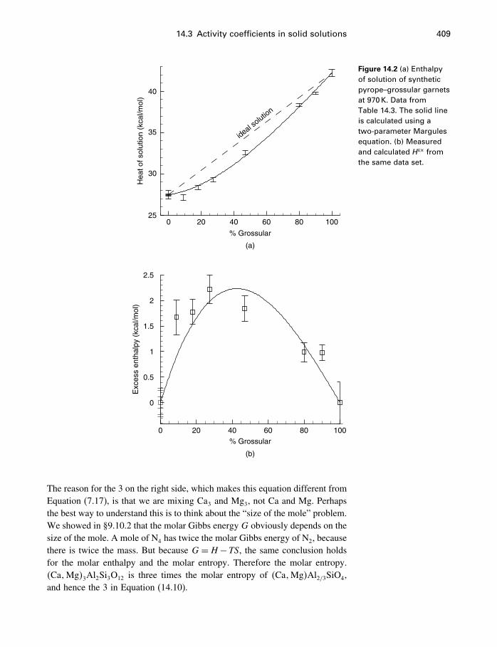
14.3 Activity coefficients in solid solutions 409
% Grossular
Hea
t of s
olut
ion
(kca
l/mol
)
0 20 40 60 80 10025
30
35
40
ideal solutio
n
(a)
% Grossular
Exc
ess
enth
alpy
(kc
al/m
ol)
0 20 40 60 80 100
0
0.5
1
1.5
2
2.5
(b)
Figure 14.2 (a) Enthalpyof solution of syntheticpyrope–grossular garnetsat 970 K. Data fromTable 14.3. The solid lineis calculated using atwo-parameter Margulesequation. (b) Measuredand calculated Hex fromthe same data set.
The reason for the 3 on the right side, which makes this equation different fromEquation (7.17), is that we are mixing Ca3 and Mg3, not Ca and Mg. Perhapsthe best way to understand this is to think about the “size of the mole” problem.We showed in §9.10.2 that the molar Gibbs energy G obviously depends on thesize of the mole. A mole of N4 has twice the molar Gibbs energy of N2, becausethere is twice the mass. But because G=H−TS, the same conclusion holdsfor the molar enthalpy and the molar entropy. Therefore the molar entropy.�Ca�Mg�3Al2Si3O12 is three times the molar entropy of �Ca�Mg�Al2/3SiO4,and hence the 3 in Equation (14.10).
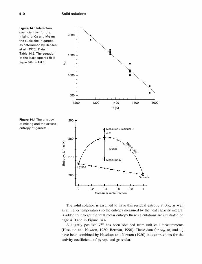
410 Solid solutions
Figure 14.3 Interactioncoefficient wG for themixing of Ca and Mg onthe cubic site in garnet,as determined by Hensenet al. (1975). Data inTable 14.2. The equationof the least squares fit iswG = 7460−4�3T .
T (K)
wG
1200 1300 1400 1500 1600
500
1000
1500
2000
Figure 14.4 The entropyof mixing and the excessentropy of garnets.
290
280
270
260
Ent
ropy
, J/(
mol
K)
Pyrope
Measured S
Measured + residual S
–12.278
4.51
Ideal mixing
Grossular
Grossular mole fraction0 0.2 0.4 0.6 0.8 1
The solid solution is assumed to have this residual entropy at 0K, as wellas at higher temperatures so the entropy measured by the heat capacity integralis added to it to get the total molar entropy.these calculations are illustrated onpage 410 and in Figure 14.4.
A slightly positive V ex has been obtained from unit call measurements(Haselton and Newton, 1980; Berman, 1990). These data for wH�ws and wvhave been combined by Haselton and Newton (1980) into expressions for theactivity coefficients of pyrope and grossular.
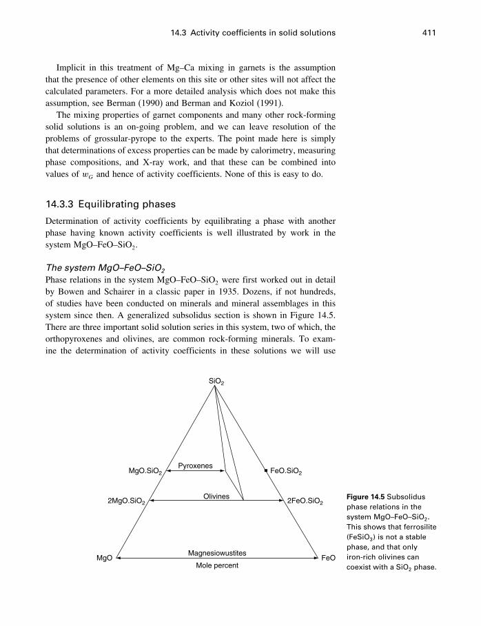
14.3 Activity coefficients in solid solutions 411
Implicit in this treatment of Mg–Ca mixing in garnets is the assumptionthat the presence of other elements on this site or other sites will not affect thecalculated parameters. For a more detailed analysis which does not make thisassumption, see Berman (1990) and Berman and Koziol (1991).
The mixing properties of garnet components and many other rock-formingsolid solutions is an on-going problem, and we can leave resolution of theproblems of grossular-pyrope to the experts. The point made here is simplythat determinations of excess properties can be made by calorimetry, measuringphase compositions, and X-ray work, and that these can be combined intovalues of wG and hence of activity coefficients. None of this is easy to do.
14.3.3 Equilibrating phases
Determination of activity coefficients by equilibrating a phase with anotherphase having known activity coefficients is well illustrated by work in thesystem MgO–FeO–SiO2.
The system MgO–FeO–SiO2
Phase relations in the system MgO–FeO–SiO2 were first worked out in detailby Bowen and Schairer in a classic paper in 1935. Dozens, if not hundreds,of studies have been conducted on minerals and mineral assemblages in thissystem since then. A generalized subsolidus section is shown in Figure 14.5.There are three important solid solution series in this system, two of which, theorthopyroxenes and olivines, are common rock-forming minerals. To exam-ine the determination of activity coefficients in these solutions we will use
SiO2
MgO.SiO2 FeO.SiO2
2MgO.SiO2 2FeO.SiO2
MgO
Pyroxenes
Olivines
Magnesiowustites
Mole percentFeO
Figure 14.5 Subsolidusphase relations in thesystem MgO–FeO–SiO2.This shows that ferrosilite(FeSiO3) is not a stablephase, and that onlyiron-rich olivines cancoexist with a SiO2 phase.
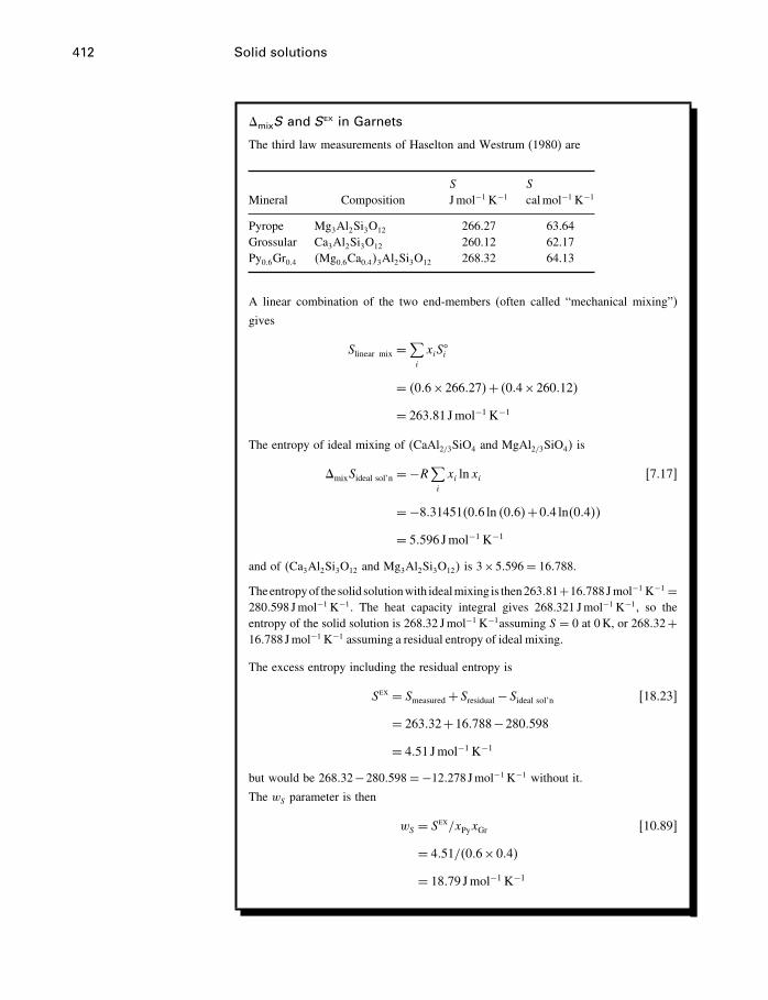
412 Solid solutions
�mixS and Sex in Garnets
The third law measurements of Haselton and Westrum (1980) are
S S
Mineral Composition Jmol−1 K−1 calmol−1 K−1
Pyrope Mg3Al2Si3O12 266.27 63.64Grossular Ca3Al2Si3O12 260.12 62.17Py0�6Gr0�4 �Mg0�6Ca0�4�3Al2Si3O12 268.32 64.13
A linear combination of the two end-members (often called “mechanical mixing”)
gives
Slinear mix =∑i
xiS�i
= �0�6×266�27�+ �0�4×260�12�
= 263�81 Jmol−1 K−1
The entropy of ideal mixing of �CaAl2/3SiO4 and MgAl2/3SiO4� is
�mixSideal sol’n =−R∑i
xi ln xi [7.17]
=−8�31451�0�6 ln �0�6�+0�4 ln�0�4��
= 5�596 Jmol−1 K−1
and of �Ca3Al2Si3O12 and Mg3Al2Si3O12� is 3×5�596= 16�788.
Theentropyof the solid solutionwith idealmixing is then263�81+16�788 Jmol−1 K−1 =280�598 Jmol−1 K−1. The heat capacity integral gives 268.321 Jmol−1 K−1, so theentropy of the solid solution is 268.32 Jmol−1 K−1assuming S = 0 at 0K, or 268�32+16�788 Jmol−1 K−1 assuming a residual entropy of ideal mixing.
The excess entropy including the residual entropy is
Sex = Smeasured +Sresidual−Sideal sol’n [18.23]
= 263�32+16�788−280�598
= 4�51 Jmol−1 K−1
but would be 268�32−280�598=−12�278 Jmol−1 K−1 without it.
The wS parameter is then
wS = Sex/xPyxGr [10.89]
= 4�51/�0�6×0�4�
= 18�79 Jmol−1 K−1
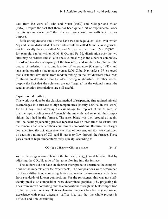
14.3 Activity coefficients in solid solutions 413
data from the work of Hahn and Muan (1962) and Nafziger and Muan(1967). Despite the fact that there has been quite a bit of experimental workon this system since 1967 the data we have chosen are sufficient for ourpurpose.
Both orthopyroxene and olivine have two nonequivalent sites over whichMg and Fe are distributed. The two sites could be called X and Y as in garnets,but historically they are called M1 and M2, so that pyroxene [�Mg�Fe�SiO3],for example, can be written M1M2Si2O6, and Fe–Mg distribution over the twosites may be ordered (most Fe in one site, most Mg in the other) or completelydisordered (random occupancy of the two sites), and similarly for olivine. Thedegree of ordering is a strong function of temperature (Ganguly, 1982), andsubstantial ordering may remain even at 1200 �C, but Navrotsky (1971) showedthat substantial deviations from random mixing on the two different sites leadsto almost no deviation from the ideal mixing relationships. In other words,despite the fact that the solutions are not “regular” in the original sense, theregular solution formulations are still useful.
Experimental method
This work was done by the classical method of suspending fine-grained mineralassemblages in a furnace at high temperatures (mostly 1200 �C in this work)for 1–14 days, then allowing the assemblage to drop out of the furnace, sothat the rapid cooling would “quench” the minerals and so retain the compo-sitions they had in the furnace. The assemblage was then ground up again,and the heating/quenching process repeated two or three times to ensure thatthe minerals had reached their equilibrium compositions. Because the chargescontained iron the oxidation state was a major concern, and this was controlledby causing a mixture of CO2 and H2 gases to flow through the furnace. Thesegases react at high temperatures very quickly, according to
CO2�g�+2H2�g�= CH4�g�+O2�g� (14.11)
so that the oxygen atmosphere in the furnace (the fO2) could be controlled by
adjusting the CO2/H2 ratio of the gases flowing into the furnace.The authors did not have an electron microprobe to determine the composi-
tions of the minerals after the experiments. The compositions were determinedby X-ray diffraction, comparing lattice parameter measurements with thosefrom standards of known composition. For the pyroxenes, this was not suffi-ciently precise, so compositions were determined graphically by projecting tielines from known coexisting olivine compositions through the bulk compositionto the pyroxene boundary. This explanation may not be clear if you have noexperience with phase diagrams; suffice it to say that the whole process isdifficult and time-consuming.
414 Solid solutions
Pyroxene solid solutionsThe activity of the FeSiO3 component of the MgSiO3–FeSiO3 (enstatite–ferrosilite) solid solution was obtained by using as experimental charges com-positions in this series plus silica plus Fe metal, in the furnace atmospherehaving the controlled fO2
as described above. The relevant reaction is
�FeSiO3�in px ss = Fe+SiO2+ 1
2O2�g� (14.12)
for which the equilibrium constant is
aFeaSiO2a1/2O2
aFeSiO3
= K
With aFe and aSiO2fixed at 1.0 by the presence of the pure solid phases (SiO2
is undoubtedly in the form of tridymite, but is not explicitly mentioned), thiscan be rewritten
12 ln fO2
− ln �xFeSiO3FeSiO3
�= −�rG�
RT(14.13)
Using the function (Equation 10.116) the activity coefficient of FeSiO3 canbe written
ln �FeSiO3�= x2MgSiO3
Inserting this into Equation (14.13),
12 ln fO2
− ln �xFeSiO3�= −�rG
�
RT−x2MgSiO3
(14.14)
If �rG� is known, measured pyroxene compositions and fO2
values allowcalculation of . If �rG
� is to be determined as well, we note that (14.14) isan equation in the form y = ax+b, where
y = 12 ln fO2
− ln �xFeSiO3�
x = x2MgSiO3
Therefore a plot of 12 ln fO2
− ln �xFeSiO3� versus x2MgSiO3
will give a slope of and an intercept of −�rG
�/RT .The results showed that aFeSiO3
and xFeSiO3were the same, within experi-
mental precision. More exactly, they found that = 0�07±0�12, which is notsignificantly different from the ideal value of zero.
Magnesiowüstite solid solutionsThe activities of FeO in solid solutions of FeO and MgO were obtained at1100 � and 1300 �C by Hahn and Muan (1962). The method was similar to thatfor the pyroxene solid solutions described above. Solid solutions of FeO and
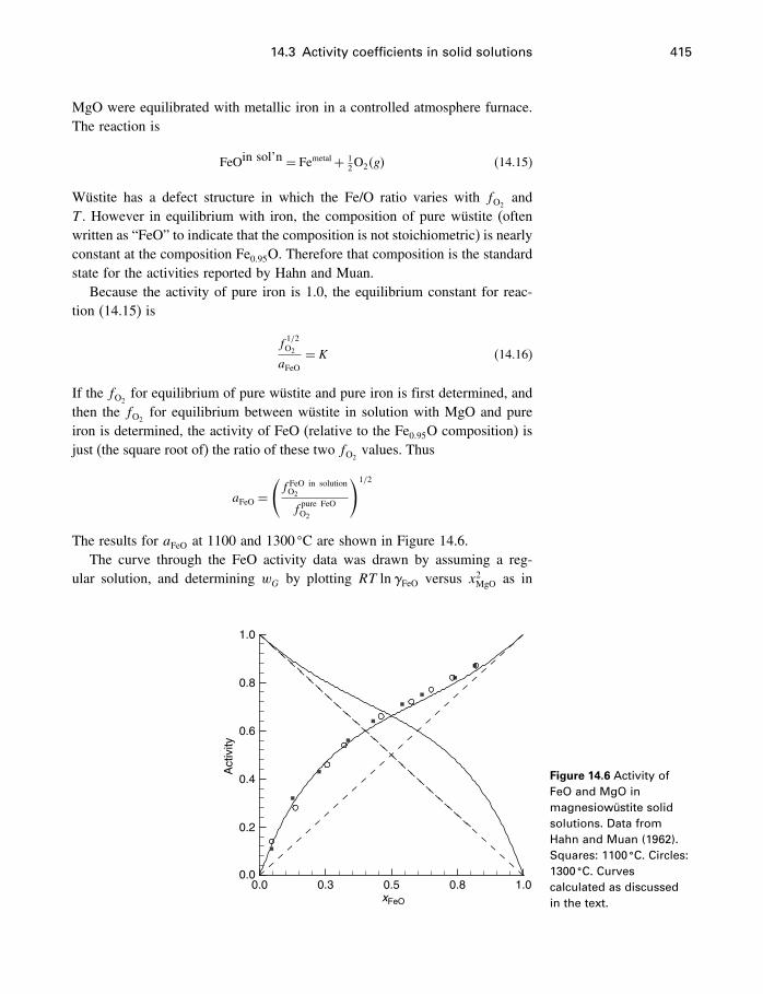
14.3 Activity coefficients in solid solutions 415
MgO were equilibrated with metallic iron in a controlled atmosphere furnace.The reaction is
FeOin sol’n = Femetal+ 12O2�g� (14.15)
Wüstite has a defect structure in which the Fe/O ratio varies with fO2and
T . However in equilibrium with iron, the composition of pure wüstite (oftenwritten as “FeO” to indicate that the composition is not stoichiometric) is nearlyconstant at the composition Fe0�95O. Therefore that composition is the standardstate for the activities reported by Hahn and Muan.
Because the activity of pure iron is 1.0, the equilibrium constant for reac-tion (14.15) is
f1/2O2
aFeO= K (14.16)
If the fO2for equilibrium of pure wüstite and pure iron is first determined, and
then the fO2for equilibrium between wüstite in solution with MgO and pure
iron is determined, the activity of FeO (relative to the Fe0�95O composition) isjust (the square root of) the ratio of these two fO2
values. Thus
aFeO =(f FeO in solutionO2
fpure FeOO2
)1/2
The results for aFeO at 1100 and 1300 �C are shown in Figure 14.6.The curve through the FeO activity data was drawn by assuming a reg-
ular solution, and determining wG by plotting RT lnFeO versus x2MgO as in
xFeO
Act
ivity
0.0 0.3 0.5 0.8 1.00.0
0.2
0.4
0.6
0.8
1.0
Figure 14.6 Activity ofFeO and MgO inmagnesiowüstite solidsolutions. Data fromHahn and Muan (1962).Squares: 1100 �C. Circles:1300 �C. Curvescalculated as discussedin the text.
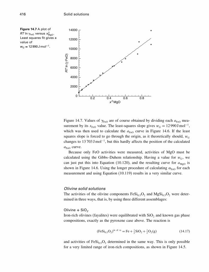
416 Solid solutions
Figure 14.7 A plot ofRT ln�FeO versus x2
MgO.Least squares fit gives avalue ofwG = 12990Jmol−1.
x 2 MgO
RT
ln(γ
FeO
)
0.2 0.4 0.6 0.80
2000
4000
6000
8000
10000
12000
14000
Figure 14.7. Values of FeO are of course obtained by dividing each aFeO mea-surement by its xFeO value. The least-squares slope gives wG = 12990 Jmol−1,which was then used to calculate the aFeO curve in Figure 14.6. If the leastsquares slope is forced to go through the origin, as it theoretically should, wGchanges to 13 703 Jmol−1, but this hardly affects the position of the calculatedaFeO curve.
Because only FeO activities were measured, activities of MgO must becalculated using the Gibbs–Duhem relationship. Having a value for wG, wecan just put this into Equation (10.120), and the resulting curve for aMgO isshown in Figure 14.6. Using the longer procedure of calculating FeO for eachmeasurement and using Equation (10.119) results in a very similar curve.
Olivine solid solutionsThe activities of the olivine components FeSi0�5O2 and MgSi0�5O2 were deter-mined in three ways, that is, by using three different assemblages:
Olivine + SiO2
Iron-rich olivines (fayalites) were equilibrated with SiO2 and known gas phasecompositions, exactly as the pyroxene case above. The reaction is
�FeSi0�5O2�in ol ss = Fe+ 1
2 SiO2+ 12O2�g� (14.17)
and activities of FeSi0�5O2 determined in the same way. This is only possiblefor a very limited range of iron-rich compositions, as shown in Figure 14.5.
14.3 Activity coefficients in solid solutions 417
Olivine + pyroxeneAssemblages of olivine and pyroxene were equilibrated, and Fe and Mg dis-tributed themselves between the two solid solutions until equilibrium compo-sitions were reached. Because the elements are exchanged between the twophases, the reaction is called an exchange reaction, written
FeSiO3in px ss+MgSi0�5O2
in ol ss =MgSiO3in px ss+FeSi0�5O2
in ol ss (14.18)
and the equilibrium constant expression is
K = aMgSiO3aFeSi0�5O2
aFeSiO3aMgSi0�5O2
(14.19)
Because the pyroxenes are ideal, this can be written
K =[xMgSiO3
xFeSi0�5O2
xFeSiO3xMgSi0�5O2
]FeSi0�5O2
MgSi0�5O2
(14.20)
Now because �FeSi0�5O2/MgSi0�5O2
� must be constant, and the two terms arealso related through the Gibbs–Duhem equation (§4.14.2), they can in principlebe calculated. If we let C represent the part of (14.20) within the squarebrackets, Wagner (1952, Chapter 7) showed that
lnFeSi0�5O2=−xMgSi0�5O2
lnC−∫ MgSi0�5O2
0lnC dxMgSi0�5O2
(14.21)
and similarly for lnMgSi0�5O2. Therefore determining the coexisting olivine–
pyroxene compositions at equilibrium over a range of compositions is sufficientto determine the activity coefficients, and hence the activities, in one solidsolution series (in this case the olivines), if those in the other series (thepyroxenes) are known. The results are shown in Figure 14.8 and Table 14.4.
Olivine + magnesiowüstiteSolid solutions of olivine and magnesiowüstite were equilibrated, and Fe andMg exchanged according to the reaction
FeOin oxide+MgSi0�5Oin olivine2 =MgOin oxide+FeSi0�5O
in olivine2
and the results analyzed exactly as in the olivine + pyroxene experiments. Theonly difference is that in the pyroxene solutions the activity coefficients were1.0, while in the magnesiowüstite solutions the activity coefficients had othervalues.
Activities and mole fractions in Table 14.4 are combined to give activitycoefficients and plotted versus x2MgSi0�5O2
and x2FeSi0�5O2, respectively, just as in
Figure 14.7. The slope of the least squares fit is wG = 4785�2 Jmol−1. Note thatxFeSi0�5O2
and xMgSi0�5O2are not independent, so wG should be the same using one
or the other, and in fact they are, within experimental precision. Using bothtogether, as in Figure 14.9, gives a weighted average of the two.
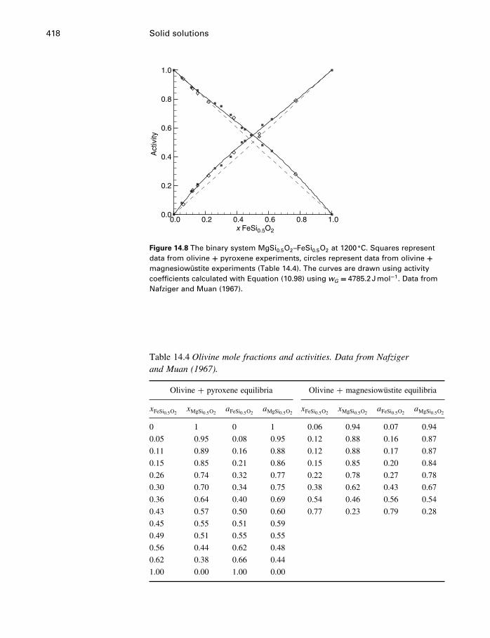
418 Solid solutions
x FeSi0.5O2
Act
ivity
0.0 0.2 0.4 0.6 0.8 1.00.0
0.2
0.4
0.6
0.8
1.0
Figure 14.8 The binary system MgSi0�5O2–FeSi0�5O2 at 1200 �C. Squares representdata from olivine + pyroxene experiments, circles represent data from olivine +magnesiowüstite experiments (Table 14.4). The curves are drawn using activitycoefficients calculated with Equation (10.98) using wG = 4785�2 J mol−1. Data fromNafziger and Muan (1967).
Table 14.4 Olivine mole fractions and activities. Data from Nafzigerand Muan (1967).
Olivine + pyroxene equilibria Olivine + magnesiowüstite equilibria
xFeSi0�5O2xMgSi0�5O2
aFeSi0�5O2aMgSi0�5O2
xFeSi0�5O2xMgSi0�5O2
aFeSi0�5O2aMgSi0�5O2
0 1 0 1 0.06 0.94 0.07 0.94
0.05 0.95 0.08 0.95 0.12 0.88 0.16 0.87
0.11 0.89 0.16 0.88 0.12 0.88 0.17 0.87
0.15 0.85 0.21 0.86 0.15 0.85 0.20 0.84
0.26 0.74 0.32 0.77 0.22 0.78 0.27 0.78
0.30 0.70 0.34 0.75 0.38 0.62 0.43 0.67
0.36 0.64 0.40 0.69 0.54 0.46 0.56 0.54
0.43 0.57 0.50 0.60 0.77 0.23 0.79 0.28
0.45 0.55 0.51 0.59
0.49 0.51 0.55 0.55
0.56 0.44 0.62 0.48
0.62 0.38 0.66 0.44
1.00 0.00 1.00 0.00
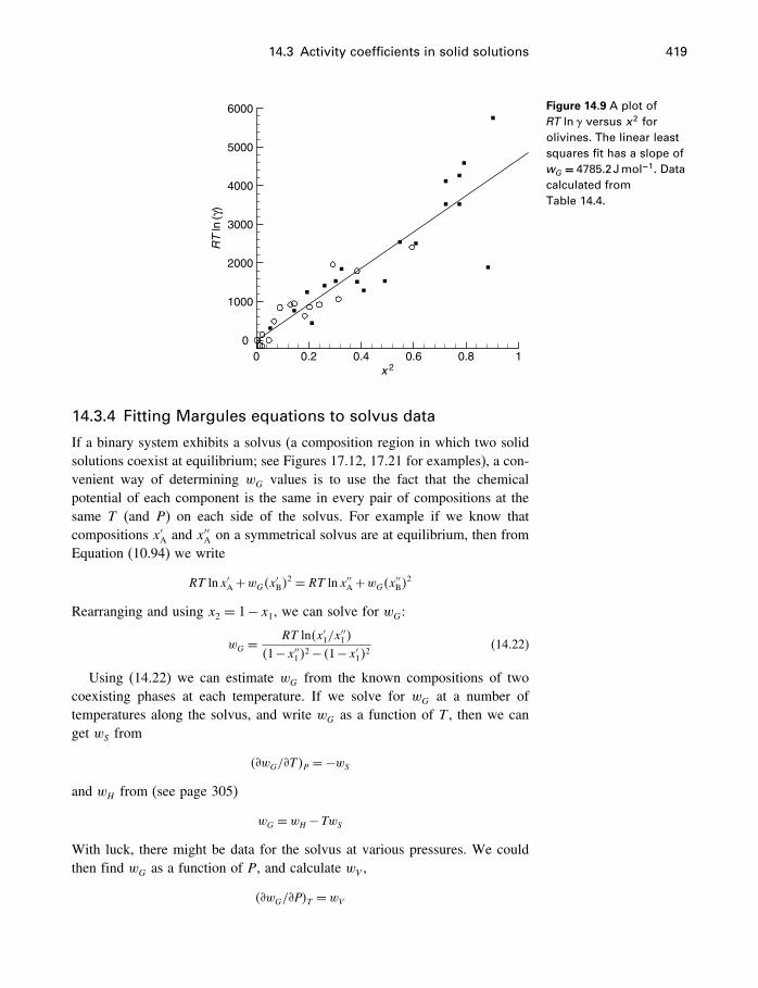
14.3 Activity coefficients in solid solutions 419
x 2
RT
ln(γ
)
0 0.2 0.4 0.6 0.8 10
1000
2000
3000
4000
5000
6000 Figure 14.9 A plot ofRT ln� versus x2 forolivines. The linear leastsquares fit has a slope ofwG = 4785�2 J mol−1. Datacalculated fromTable 14.4.
14.3.4 Fitting Margules equations to solvus data
If a binary system exhibits a solvus (a composition region in which two solidsolutions coexist at equilibrium; see Figures 17.12, 17.21 for examples), a con-venient way of determining wG values is to use the fact that the chemicalpotential of each component is the same in every pair of compositions at thesame T (and P) on each side of the solvus. For example if we know thatcompositions x′A and x′′A on a symmetrical solvus are at equilibrium, then fromEquation (10.94) we write
RT ln x′A+wG�x′B�2 = RT ln x′′A+wG�x′′B�2
Rearranging and using x2 = 1−x1, we can solve for wG:
wG = RT ln�x′1/x′′1�
�1−x′′1�2− �1−x′1�2(14.22)
Using (14.22) we can estimate wG from the known compositions of twocoexisting phases at each temperature. If we solve for wG at a number oftemperatures along the solvus, and write wG as a function of T , then we canget wS from
��wG/�T�P =−wSand wH from (see page 305)
wG = wH −TwSWith luck, there might be data for the solvus at various pressures. We couldthen find wG as a function of P, and calculate wV ,
��wG/�P�T = wV
420 Solid solutions
Alternatively, we could estimate V ex from X-ray data on the single-mineralsolid solution just above the solvus.
The more usual case, however, is that the solvus is not symmetrical, but isskewed toward one of the components. In this case we need to solve for twoMargules parameters, in order to use Equation (10.103),
Gexsol’n = x1�wG2
x1x2�+x2�wG1x1x2� [10.103]
so we need two equations. Following the same procedure as before, but thistime not converting x2 into �1−x1� we get
RT ln x′1+�2wG2−wG1
��x′2�2+2�wG1
−wG2��x′2�
3
= RT ln x′′1 + �2wG2−wG1
��x′′2�2+2�wG1
−wG2��x′′2�
3 (14.23)
RT ln x′2+�2wG1−wG2
��x′1�2+2�wG2
−wG1��x′1�
3
= RT ln x′′2 + �2wG1−wG2
��x′′1�2+2�xG2
−xG1��x′′1�
3 (14.24)
Given the compositions of the two coexisting phases, the above two equationscan be solved for wG1
and wG2. To do this you could use one of many gen-
eralized equation solvers, or use rearranged versions of (14.23) and (14.24),which give wG1
and wG2directly in terms of composition (see Thompson, 1967,
p. 355 and Eugster et al., 1972, p. 164, for examples). For additional details andexamples of applications to mineral systems, see Thompson and Waldbaum(1968, 1969), and Waldbaum and Thompson (1968, 1969).
14.4 Summary
We need to know which way reactions will go when solutions are involved,such as minerals dissolving/precipitating, or electrolytes dissociating. We havea thermodynamic potential (the Gibbs energy) which fills this role for purephases, so we just need to know how to determine it for dissolved substances.In addition, we need to know how it changes with T , P, and composition of thesolution, which involves knowing how to determine the temperature, pressure,and compositional derivatives of this quantity.
Excess properties, the difference between the property in a real solution andin an ideal solution, are generally expressed as a relative or relative partialmolar properties, such as the relative enthalpy, L, or relative partial molarenthalpy, L. The Gibbs energy is treated differently. The fact that GT�P is athermodynamic potential leads naturally to the definition of a relative partialmolar Gibbs energy (�−��) which is not the difference from an ideal solution(�−�� is not zero even for an ideal solution) but the difference from astandard state, which in this chapter is a pure phase, but may also be somehypothetical state. The form of the equation relating �−�� to composition then
14.4 Summary 421
leads naturally to the definition of the activity, an important quantity whichessentially is what we were looking for – a compositional variable directlyrelated to the Gibbs energy of a dissolved substance.
For ideal solutions, the activity is just the mole fraction, but for non-idealsolutions, a correction factor, the activity coefficient, is introduced. Fairly sim-ple regular solution and Margules equations are then found which can expressthe variation of the excess Gibbs energy or the activity coefficients as a func-tion of concentration for nonideal solutions. These are of limited usefulness forcomplex solid solutions such as the amphiboles, and are best at systematizingrelatively simple binary solutions, fluid and solid, and when data are sufficient,ternary solutions. Beyond this, the notation gets very cumbersome, and the datarequirements become very great. Nevertheless, within its range of usefulness,the Margules approach is very useful indeed, as witnessed by the large litera-ture on the subject. Grover (1977) lists 40 publications, with brief descriptionsof their contents, which use Margules equations in mineral systems.
15Electrolyte solutions
15.1 Introduction
In dealing with the thermodynamic properties of ions we have one difficultyin addition to those encountered in dealing with compounds and elements. Forcompounds and elements we found that although we could measure absolutevalues for some properties, others such as enthalpy and the other energy termscontained an undetermined constant. We got around this by using the conceptof “formation from the elements.” It would of course be very convenient to alsohave thermodynamic properties of individual ions, but because positively andnegatively charged ions cannot be separated from each other to any significantextent, their individual properties cannot be measured. To get around this, weneed an additional convention, while retaining the formation from the elementsconvention.
In the following section we discuss the problems of activities of ionicspecies. Following that we discuss the conventions used to obtain numericalvalues for the state variables of individual ions, and we discuss the theoryunderlying the two major approaches to systematizing the data on electrolytes,the HKF and the Pitzer models. Because these are essentially equations of state,we introduced them in Chapter 13 (§13.6.2 and §13.6.3).
15.2 Activities of electrolyte components
15.2.1 Fugacity versus concentration for electrolytes
An electrolyte is a compound that splits up into charged particles when dis-solved in water. For example, halite, NaCl, splits up into Na+ and Cl− particles(ions) in solution. What would you expect to be the consequences of this foractivity and fugacity? To examine this let’s consider the compound AB whichsplits up into particles A and B in solution. But before doing that, we shouldthink about what we expect the relationship to be.
What to expectIn §8.2.3 we defined the standard state for solute i as the ideal (�
i = 1) onemolal (m�
i = 1) solution. One consequence of this is that as mi → 0, i → 1,
422
15.2 Activities of electrolyte components 423
and ai → mi. To simplify, we just say that in dilute solutions, ai = mi. If wewere able to determine the fugacity of i in these solutions, we might not botherwith this kind of standard state; we could use ai = fi/f �
i , as we do for gases.But just because fi/f
�i is not useful doesn’t mean it is not true. If f �
i is thefugacity of i in an ideal one molal solution, and fi is the fugacity of i in someother solution at the same T , then
ai = fi/f �i= �mii�/�m�
i �i �
so that in general
fi = f �i aiand in very dilute solutions where i/�m
�i
�i �= 1,
fi = f �i miIn other words, f �
i is the (Henry’s law) constant of proportionality for fi ∝ ai,or fi ∝ mi in very dilute solutions. So we expect fugacity to be directly pro-portional to concentration in dilute solutions.
What we getNow consider electrolyte AB, which dissociates into particles A and B. Forthe moment it doesn’t matter whether they are electrically charged or not. Ingeneral, there will be an equilibrium constant for the reaction AB� = A+B,and we can write an equilibrium constant for this (dispensing with activitycoefficients for the moment, which just complicate but do not change the pointwe are getting at),
K1 =mA ·mB
mAB�and, because mA =mB�
= m2A
mAB�
where we use mAB for the analytical concentration, that is, the result of ana-lyzing the solution for AB (in this case, this is component AB), and mAB�
for the concentration of species AB in solution, where, because mA = mB,mAB = mAB� +mA (or mAB = mAB� +mB). We can also suppose that in thevapor phase above the solution, the vapor pressure or fugacity of AB, fAB, isproportional to mAB� (not to mAB, because some of AB has become A and B).Thus Henry’s law gives
fAB ∝mAB�
= K2 ·mAB�
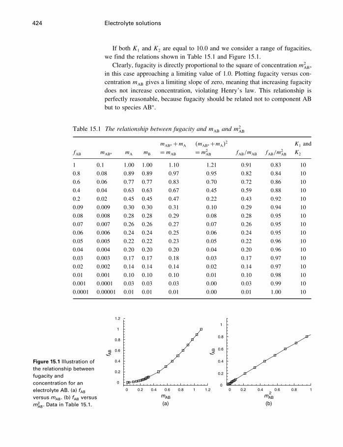
424 Electrolyte solutions
If both K1 and K2 are equal to 10.0 and we consider a range of fugacities,we find the relations shown in Table 15.1 and Figure 15.1.
Clearly, fugacity is directly proportional to the square of concentration m2AB,
in this case approaching a limiting value of 1.0. Plotting fugacity versus con-centration mAB gives a limiting slope of zero, meaning that increasing fugacitydoes not increase concentration, violating Henry’s law. This relationship isperfectly reasonable, because fugacity should be related not to component ABbut to species AB�.
Table 15.1 The relationship between fugacity and mAB and m2AB
fAB mAB� mA mB
mAB� +mA
=mAB
�mAB� +mA�2
=m2AB fAB/mAB fAB/m
2AB
K1 and
K2
1 0�1 1�00 1�00 1�10 1�21 0�91 0�83 10
0.8 0�08 0�89 0�89 0�97 0�95 0�82 0�84 10
0.6 0�06 0�77 0�77 0�83 0�70 0�72 0�86 10
0.4 0�04 0�63 0�63 0�67 0�45 0�59 0�88 10
0.2 0�02 0�45 0�45 0�47 0�22 0�43 0�92 10
0.09 0�009 0�30 0�30 0�31 0�10 0�29 0�94 10
0.08 0�008 0�28 0�28 0�29 0�08 0�28 0�95 10
0.07 0�007 0�26 0�26 0�27 0�07 0�26 0�95 10
0.06 0�006 0�24 0�24 0�25 0�06 0�24 0�95 10
0.05 0�005 0�22 0�22 0�23 0�05 0�22 0�96 10
0.04 0�004 0�20 0�20 0�20 0�04 0�20 0�96 10
0.03 0�003 0�17 0�17 0�18 0�03 0�17 0�97 10
0.02 0�002 0�14 0�14 0�14 0�02 0�14 0�97 10
0.01 0�001 0�10 0�10 0�10 0�01 0�10 0�98 10
0.001 0�0001 0�03 0�03 0�03 0�00 0�03 0�99 10
0.0001 0�00001 0�01 0�01 0�01 0�00 0�01 1�00 10
Figure 15.1 Illustration ofthe relationship betweenfugacity andconcentration for anelectrolyte AB. (a) fAB
versus mAB. (b) fAB versusm2
AB. Data in Table 15.1.
mAB
f AB
0
0
0.2
0.2
0.4
0.4
0.6
0.6
0.8
0.8
1
1
1.2
0
0.2
0.4
0.6
0.8
1
f AB
1.2 0 0.2 0.4 0.6 0.8 1
(a)
mAB2
(b)
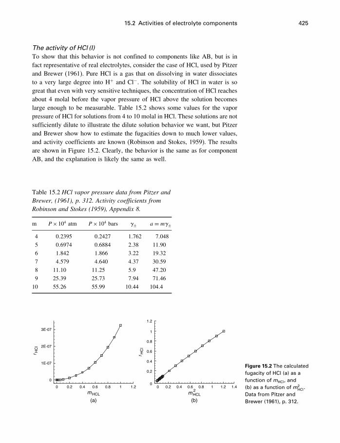
15.2 Activities of electrolyte components 425
The activity of HCl (I)To show that this behavior is not confined to components like AB, but is infact representative of real electrolytes, consider the case of HCl, used by Pitzerand Brewer (1961). Pure HCl is a gas that on dissolving in water dissociatesto a very large degree into H+ and Cl−. The solubility of HCl in water is sogreat that even with very sensitive techniques, the concentration of HCl reachesabout 4 molal before the vapor pressure of HCl above the solution becomeslarge enough to be measurable. Table 15.2 shows some values for the vaporpressure of HCl for solutions from 4 to 10 molal in HCl. These solutions are notsufficiently dilute to illustrate the dilute solution behavior we want, but Pitzerand Brewer show how to estimate the fugacities down to much lower values,and activity coefficients are known (Robinson and Stokes, 1959). The resultsare shown in Figure 15.2. Clearly, the behavior is the same as for componentAB, and the explanation is likely the same as well.
Table 15.2 HCl vapor pressure data from Pitzer andBrewer, (1961), p. 312. Activity coefficients fromRobinson and Stokes (1959), Appendix 8.
m P×104 atm P×104 bars ± a=m±4 0�2395 0�2427 1�762 7�048
5 0�6974 0�6884 2�38 11�90
6 1�842 1�866 3�22 19�32
7 4�579 4�640 4�37 30�59
8 11�10 11�25 5�9 47�20
9 25�39 25�73 7�94 71�46
10 55�26 55�99 10�44 104�4
(b)
3E-07
2E-07
1E-07
f HC
l
f HC
l
0
00
0.2
0.2
0.4
0.4
0.6
mHCL
0.6
0.8
0.8
1
1
1.2 0 0.2
mHCL2
0.4 0.6 0.8 1 1.2 1.4
1.2
(a)
Figure 15.2 The calculatedfugacity of HCl (a) as afunction of mHCl, and(b) as a function of m2
HCl.Data from Pitzer andBrewer (1961), p. 312.
426 Electrolyte solutions
15.2.2 The activity of electrolytes
So we find that f ∝ m2 for a binary electrolyte like HCl or NaCl. In dilutesolutions then,
fHCl = f �HClm2HCl
or in general,
fHCl = f �HCl�±m2HCl�
and
aHCl = fHCl/f �HCl= ±m2
HCl (15.1)
where ± is a new kind of activity coefficient to be discussed below.If we went through the same procedure for an electrolyte which dissoci-
ates into three ions (e.g., Na2SO4) we would find f ∝ m3, and for four ions(e.g., AlCl3) we would find f ∝m4, and so on, so that for example,
aAlCl3 = ±m4AlCl3
In very dilute solutions, HCl is completely dissociated – the concentrationof HCl� is undetectable, and ± = 1, so
aHCl =m2HCl
Obviously we could get the same results, mathematically, not by squaring theconcentration, but by taking the square root of the activity,
a1/2HCl =mHCl
This raises an interesting question.
15.2.3 Choice of solute component
Before going on to define single ion activities and activity coefficients, let’spause to reflect on the similarity between the case considered here (a com-pletely dissociated electrolyte in water), and the olivine solid solution caseconsidered in Chapter 9 (§9.10.2). The physical systems are completely differ-ent, but the thermodynamic problem is almost identical, the only significantdifference being that in the olivine case the concentrations were measured bymole fractions and ideality consisted in conforming to Raoult’s law, while here
15.2 Activities of electrolyte components 427
concentrations are measured in molality and ideality is represented by Henry’slaw. Apart from that, the problem in both cases consists in choosing a solutecomponent that is appropriate to the situation.
In Chapter 9 we showed the purely formal relation between componentactivities
ai = �a0�5i�2
and showed that in the case of Mg2SiO4–Fe2SiO4 solid solutions, the activityof component Mg2SiO4 would plot as a parabolic curve versus mole fraction,while component MgSi0�5O2 would come close to plotting as a straight line. Inthe HCl–H2O case we find that component HCl is strongly curved on a plotof f (or a) versus m, but gives a straight line when plotted versus m2. We areentitled to ask why, in the case of HCl, did we not behave consistently andplot component H0�5Cl0�5 versus m instead of changing the concentration axisfrom m to m2? Obviously aH0�5Cl0�5
versus mHCl would result in a straight linetoo, because aH0�5Cl0�5
= a1/2HCl�
We can answer this in two ways. First, we will introduce and use componentH0�5Cl0�5 (and analogous components for other compounds), but it is given aspecial symbol �a±� for reasons that will become apparent. The other way toanswer the question is to point out that although we need no knowledge ofthe molecular nature of a system to be able to apply thermodynamics to it, wewould be silly to ignore such knowledge when it is available. Our rationalefor using m2 rather than m is based on overwhelming experimental evidencethat many binary electrolytes split completely into two particles on dissolvingin water. This provides the reason why aHCl versus m
2HCl works better than
aHCl versus mHCl, just as the observation that Mg and Fe effectively occupy asingle crystallographic site in olivine provides the reason why aMgSi0�5O2
versusx works better than aMg2SiO4
versus x. Thermodynamics doesn’t care whichcomponent we use, but points out that if we are pleased by aHCl versus m
2HCl,
we can get the same results from aH0�5Cl0�5versus mHCl�
In general then, we see again that the choice of components is an importantpart of any thermodynamically based analysis or theory. Certain choices will“work better” or be more appropriate than others, and there will always be areason for this. Although the reason may be that the component correspondsclosely to the actual chemical species (N2 certainly works better than N4 in gasmixture equations), this is not necessarily the case as we have seen in both theolivine and HCl–H2O examples.
15.2.4 Activity of HCl (II)
To develop the relationships shown in Figure 15.2 we relied on some ratherhypothetical fugacity calculations. This helps to understand the relationships,but of course real, measured activities show the same thing. In Figure 15.3 is
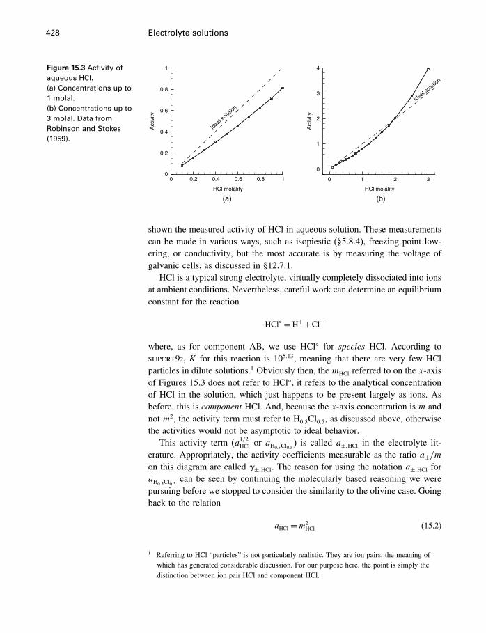
428 Electrolyte solutions
Figure 15.3 Activity ofaqueous HCl.(a) Concentrations up to1 molal.(b) Concentrations up to3 molal. Data fromRobinson and Stokes(1959).
HCl molality
Act
ivity
00
0.2
0.2
0.4
0.4
0.6
Ideal
solut
ion
0.6
0.8
0.8 1
1
(a)HCl molality
Act
ivity
Ideal solutio
n
0 1 2 3
0
1
2
3
4
(b)
shown the measured activity of HCl in aqueous solution. These measurementscan be made in various ways, such as isopiestic (§5.8.4), freezing point low-ering, or conductivity, but the most accurate is by measuring the voltage ofgalvanic cells, as discussed in §12.7.1.
HCl is a typical strong electrolyte, virtually completely dissociated into ionsat ambient conditions. Nevertheless, careful work can determine an equilibriumconstant for the reaction
HCl� = H++Cl−
where, as for component AB, we use HCl� for species HCl. According tosupcrt92, K for this reaction is 105�13, meaning that there are very few HClparticles in dilute solutions.1 Obviously then, the mHCl referred to on the x-axisof Figures 15.3 does not refer to HCl�, it refers to the analytical concentrationof HCl in the solution, which just happens to be present largely as ions. Asbefore, this is component HCl. And, because the x-axis concentration is m andnot m2, the activity term must refer to H0�5Cl0�5, as discussed above, otherwisethe activities would not be asymptotic to ideal behavior.
This activity term (a1/2HCl or aH0�5Cl0�5) is called a±�HCl in the electrolyte lit-
erature. Appropriately, the activity coefficients measurable as the ratio a±/mon this diagram are called ±�HCl. The reason for using the notation a±�HCl foraH0�5Cl0�5
can be seen by continuing the molecularly based reasoning we werepursuing before we stopped to consider the similarity to the olivine case. Goingback to the relation
aHCl =m2HCl (15.2)
1 Referring to HCl “particles” is not particularly realistic. They are ion pairs, the meaning ofwhich has generated considerable discussion. For our purpose here, the point is simply thedistinction between ion pair HCl and component HCl.
15.2 Activities of electrolyte components 429
which holds for infinitely dilute solutions, we can next write
aHCl =mH+mCl− (15.3)
for the same conditions, because each mole of HCl breaks down completelyto H+ and Cl−. At this point we introduce the concept of activity coefficientsfor individual ions, and define them such that they approach 1.0 in infinitelydilute solutions, just as we did with the activity coefficients of undissociatedsolutes. They are a useful mental concept in spite of not being measurable. Atinfinite dilution, then,
H+ = Cl− = 1�0
and under other conditions they take on values such that
aHCl = �mH+H+��mCl−Cl−� (15.4)
remains true. Therefore
aHCl = aH+aCl− (15.5)
or
aH+aCl−/aHCl = 1�0 (15.6)
This defines the equilibrium constant for the reaction between com-ponent HCl and the ions H+ and Cl−. It follows then that for thereaction
HCl �not HCl��= H++Cl−; �rG� = 0 (15.7)
As usual, it is best to see the truth of a relationship by understanding it ratherthan by seeing no fault with its derivation. In this case this can be accomplishedby realizing that in the ideal one molal standard state to which �rG
� refers, thesolute component HCl consists in solution entirely as H+ and Cl−, thereforethe G of component HCl has no choice but to be identical to GH+ +GCl− ,from which it follows that �rG
� = 0� Pitzer (1995, p. 206) discusses a similarcase, the hydration of aqueous NH3 to NH4OH, which happens to a small andunknown extent, i.e.,
NH3�aq�+H2O�l�= NH4OH�aq�
The activity of species NH4OH� is unknown, so NH4OH is considered a
component, which of course is equal to the known amount of NH3 in solution,so as before, K = 1 and �rG
� = 0. Another case is the hydration of dissolvedCO2, discussed in §9.10.
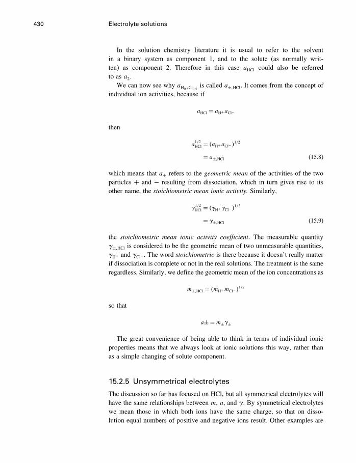
430 Electrolyte solutions
In the solution chemistry literature it is usual to refer to the solventin a binary system as component 1, and to the solute (as normally writ-ten) as component 2. Therefore in this case aHCl could also be referredto as a2�
We can now see why aH0�5Cl0�5is called a±�HCl. It comes from the concept of
individual ion activities, because if
aHCl = aH+aCl−
then
a1/2HCl = �aH+aCl−�
1/2
= a±�HCl (15.8)
which means that a± refers to the geometric mean of the activities of the twoparticles + and − resulting from dissociation, which in turn gives rise to itsother name, the stoichiometric mean ionic activity. Similarly,
1/2HCl = �H+Cl−�
1/2
= ±�HCl (15.9)
the stoichiometric mean ionic activity coefficient. The measurable quantity±�HCl is considered to be the geometric mean of two unmeasurable quantities,H+ and Cl− . The word stoichiometric is there because it doesn’t really matterif dissociation is complete or not in the real solutions. The treatment is the sameregardless. Similarly, we define the geometric mean of the ion concentrations as
m±�HCl = �mH+mCl−�1/2
so that
a±=m±±
The great convenience of being able to think in terms of individual ionicproperties means that we always look at ionic solutions this way, rather thanas a simple changing of solute component.
15.2.5 Unsymmetrical electrolytes
The discussion so far has focused on HCl, but all symmetrical electrolytes willhave the same relationships between m, a, and . By symmetrical electrolyteswe mean those in which both ions have the same charge, so that on disso-lution equal numbers of positive and negative ions result. Other examples are
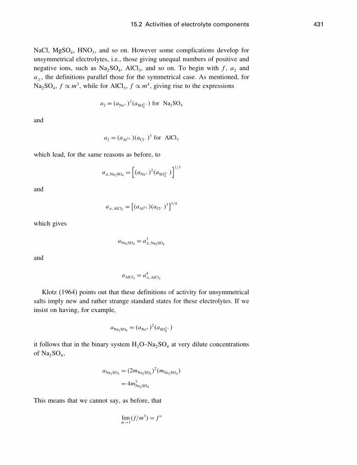
15.2 Activities of electrolyte components 431
NaCl, MgSO4, HNO3, and so on. However some complications develop forunsymmetrical electrolytes, i.e., those giving unequal numbers of positive andnegative ions, such as Na2SO4, AlCl3, and so on. To begin with f , a2 anda±, the definitions parallel those for the symmetrical case. As mentioned, forNa2SO4, f ∝m3, while for AlCl3, f ∝m4, giving rise to the expressions
a2 = �aNa+�2�aSO2−4� for Na2SO4
and
a2 = �aAl3+��aCl−�3 for AlCl3
which lead, for the same reasons as before, to
a±�Na2SO4=[�aNa+�
2�aSO2−4�]1/3
and
a±�AlCl3 =[�aAl3+��aCl−�
3]1/4
which gives
aNa2SO4= a3±�Na2SO4
and
aAlCl3 = a4±�AlCl3
Klotz (1964) points out that these definitions of activity for unsymmetricalsalts imply new and rather strange standard states for these electrolytes. If weinsist on having, for example,
aNa2SO4= �aNa+�2�aSO2−
4�
it follows that in the binary system H2O–Na2SO4 at very dilute concentrationsof Na2SO4�
aNa2SO4= �2mNa2SO4
�2�mNa2SO4�
= 4m3Na2SO4
This means that we cannot say, as before, that
limm→1
�f/m3�= f �
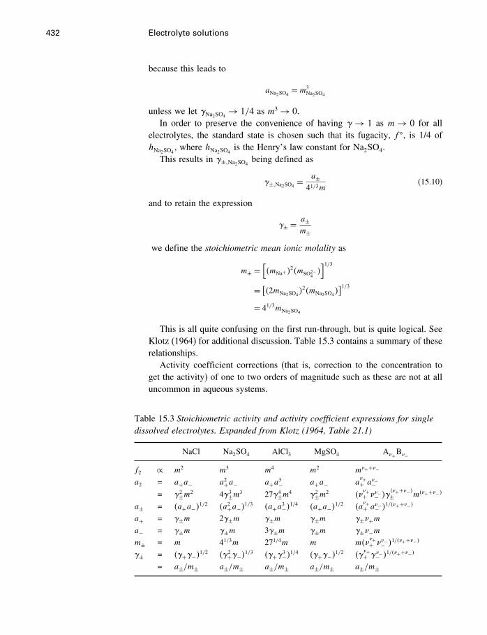
432 Electrolyte solutions
because this leads to
aNa2SO4=m3
Na2SO4
unless we let Na2SO4→ 1/4 as m3 → 0.
In order to preserve the convenience of having → 1 as m→ 0 for allelectrolytes, the standard state is chosen such that its fugacity, f �, is 1/4 ofhNa2SO4
, where hNa2SO4is the Henry’s law constant for Na2SO4.
This results in ±�Na2SO4being defined as
±�Na2SO4= a±
41/3m(15.10)
and to retain the expression
± = a±m±
we define the stoichiometric mean ionic molality as
m± =[�mNa+�
2�mSO2−4�]1/3
= [�2mNa2SO4�2�mNa2SO4
�]1/3
= 41/3mNa2SO4
This is all quite confusing on the first run-through, but is quite logical. SeeKlotz (1964) for additional discussion. Table 15.3 contains a summary of theserelationships.
Activity coefficient corrections (that is, correction to the concentration toget the activity) of one to two orders of magnitude such as these are not at alluncommon in aqueous systems.
Table 15.3 Stoichiometric activity and activity coefficient expressions for singledissolved electrolytes. Expanded from Klotz (1964, Table 21.1)
NaCl Na2SO4 AlCl3 MgSO4 A�+B�−
f2 ∝ m2 m3 m4 m2 m�++�−
a2 = a+a− a2+a− a+a3− a+a− a�++ a�−−
= 2±m
2 43±m
3 274±m
4 2±m
2 ���++ ��−− �
��++�−�± m��++�−�
a± = �a+a−�1/2 �a2+a−�1/3 �a+a3−�
1/4 �a+a−�1/2 �a�++ a�−− �
1/��++�−�
a+ = ±m 2±m ±m ±m ±�+ma− = ±m ±m 3±m ±m ±�−mm± = m 41/3m 271/4m m m��
�++ ��−− �
1/��++�−�
± = �+−�1/2 �2+−�
1/3 �+3−�
1/4 �+−�1/2 ��++ �−− �
1/��++�−�
= a±/m± a±/m± a±/m± a±/m± a±/m±
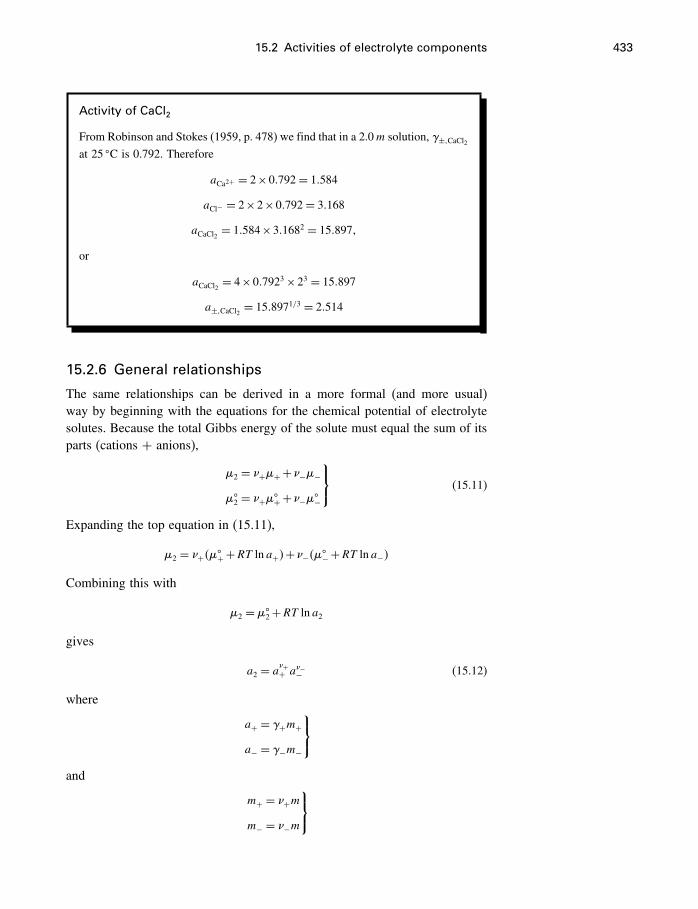
15.2 Activities of electrolyte components 433
Activity of CaCl2
From Robinson and Stokes (1959, p. 478) we find that in a 2.0m solution, ±�CaCl2at 25 �C is 0.792. Therefore
aCa2+ = 2×0�792= 1�584
aCl− = 2×2×0�792= 3�168
aCaCl2 = 1�584×3�1682 = 15�897�
or
aCaCl2 = 4×0�7923×23 = 15�897
a±�CaCl2 = 15�8971/3 = 2�514
15.2.6 General relationships
The same relationships can be derived in a more formal (and more usual)way by beginning with the equations for the chemical potential of electrolytesolutes. Because the total Gibbs energy of the solute must equal the sum of itsparts (cations + anions),
�2 = �+�++�−�−
��2 = �+��
+ +�−��−
⎫⎬⎭ (15.11)
Expanding the top equation in (15.11),
�2 = �+���+ +RT lna+�+�−���
− +RT lna−�
Combining this with
�2 = ��2+RT lna2
gives
a2 = a�++ a�−− (15.12)
where
a+ = +m+
a− = −m−
⎫⎬⎭and
m+ = �+mm− = �−m
⎫⎬⎭
434 Electrolyte solutions
Dividing by � (where � = �++�−) gives an average �2 and ��2, so
�2/� = ��2/�+RT ln�a�++ a
�−− �
1/�
Then defining
�± = ���++ ·��−− �1v
��± = ����+
+ ·���−− �
1v
a± = �a�++ ·a�−− �1v
⎫⎪⎪⎪⎬⎪⎪⎪⎭ (15.13)
we get
�± = ��± +RT lna± (15.14)
Similarly ± and m± are defined as
± = ��++ ·�−− �1�
m± = �m�++ ·m�−− �1�
⎫⎬⎭ (15.15)
The rest of the equations in Table 15.3 follow directly.
HKF notationThese relations can also be expressed generally using the notation of Helgesonet al. (1981). The terms m and ��+ +�−� in the table above are equivalent tomk and �k respectively in the following equations:
±�k =(∏
j
�j�kj
)1/�k
ak = ∏j
(j�j�kmk
)�j�k=
�k±�km
�kk
∏j
��j�kj�k
a±�k = a1/�kk
= ±�kmk
(∏j
��j�kj�k
)1/�k
where j represents the ions of component k, �j represents the stoichiometry ofion j, and
�k =∑j
�j�k
For example, if k is CaCl2,
�Ca2+ = 1� �Cl− = 2� �k = 3
15.2 Activities of electrolyte components 435
and
aCaCl2 = �Ca2+mCaCl2�1�Cl−2mCaCl2
�2
= 4�Ca2+2Cl−�m
3CaCl2
For mixtures of electrolytes, with and without common ions, the notationbecomes more complex. Helgeson et al. (1981) give the most comprehensiveset of equations available.
15.2.7 Stoichiometric versus ionic properties
The word “stoichiometric” is included in the names given a±, ±, and m± toindicate that they are derived according to the formulas given, which is moreor less equivalent to the supposition that the electrolyte dissociates completelyinto ions. If the electrolyte dissociates only partly into ions, these quantitiesmay still be derived, but they won’t represent what they have been describedas representing, i.e., the geometric mean of the properties of the free ions.
Therefore other classes of activities and activity coefficients are defined(“mean ionic activities” and “mean ionic activity coefficients,” without the“stoichiometric”), which are related to the stoichiometric quantities by thedegree of dissociation, , where
=mj/mThus
j = ·jwhere j is the mean ionic activity coefficient of the jth ion, and forcomponent k,
j ·m= j ·mj
±�k =(∏j�j�kj
) 1�k
and similarly for the other properties.We have introduced the factor to account for the degree of dissociation,
but as pointed out quite eloquently by Pitzer and Brewer (1961) in their revisionof the classic text by Lewis and Randall (1923), the value of varies with themethod used to measure it; a situation not uncommon in studies of complexphenomena controlled by molecular interactions. Therefore it is to a largeextent up to the investigator whether to use stoichiometric or ionic properties.Stoichiometric properties may be used whether or not ionic association isimportant, and have the advantage of not requiring estimates of , or theamount of complexing and ion-pairing. As we will see later in this chapter, thePitzer and HKF approaches to modeling electrolyte solutions exemplify thesetwo different methods.
436 Electrolyte solutions
15.3 Numerical values for single-ion properties
We now take a look at how numerical values are assigned to the thermodynamicproperties of single ions. There is more than one method, of course. Mostphysical chemistry courses for example will mention the MacInnes convention,which postulates that because the K+ and Cl− ions have similar properties,their activity coefficients should be identical. This means that
±�KCl = K+ = Cl−
and from this, other single ion activity coefficients can be determined. Forexample,
±�CaCl2 = �Ca2+2Cl−�
1/3
so that
Ca2+ = 3±�CaCl22±�KCl
However, this method runs into problems, such as not working well in mixedelectrolytes, and not giving coefficients compatible with Debye–Hückel coef-ficients, so it not widely used.
The usual practice is to give up any hope of determining individual ionactivities or activity coefficients, and to use conventional ones. The conventionas generally stated is that we assume all properties of the hydrogen ion tobe zero. This, combined with another convention, that the properties of theelements are zero, results in the numbers we always use. But assuming theseproperties to be zero is not really necessary. What is calculated, of course, isthe difference of an ion property from that of the hydrogen ion. Assuming theproperty of the hydrogen ion to be zero only simplifies the notation, not theconcept.
In the following discussion of single ion properties, we do not at first makeany assumptions about the properties of the elements or the hydrogen ion, butwe do define properties in terms of differences. Then we introduce the conven-tions and see how this simplifies notation. The point is that thermodynamics isnot dependent on any property being zero, only the notation is. In essence, theprocedure followed is a slight variation of the “formation from the elements”procedure discussed in Chapter 3.
It will be convenient to continue with HCl in water as our example, sothat the question becomes how do we arrive at numerical values for all thethermodynamic properties of the ions H+ and Cl−? The answer begins withthe equation for the formation of H+ and Cl− from the elements,
12H2�g�+
12Cl2�g�= H++Cl− (15.16)
15.3 Numerical values for single-ion properties 437
The standard Gibbs energy change for this reaction is found by combining datafrom three other reactions. First, the association of hydrogen and chlorine togive HCl gas has the properties
12H2�g�+
12Cl2�g�= HCl�g�
logK = 16�70; �rG� = −95299 Jmol−1
(data from Wagman et al., 1982) and the partitioning of HCl between liquidand vapor phases gives
HCl�g�= HCl�aq�
logK = 6�29; �rG� = −35929 Jmol−1
Combining these gives
12H2�g�+
12Cl2�g�= HCl�aq�
logK = 22�99; �rG� = −131228 Jmol−1
We have already shown that for the reaction
HCl�aq�= H++Cl−
logK = 1; �rG� = 0
so it follows that for the reaction we want,12H2�g�+
12Cl2�g�= H++Cl−
logK = 22�99; �rG� = −131228 Jmol−1
At this point we can go no further without making some arbitrary decision,i.e., without formulating a convention for ionic properties. The decision isbasically to define the Gibbs energy of formation of the chloride ion as
�fG�Cl− =G�
Cl− +G�H+ − 1
2G�H2
− 12G
�Cl2
(15.17)
=−131228 Jmol−1
Once this decision is made for one ion, such as Cl−, the logjam is broken andvalues for all other ions can be derived. For example, we know that
Na�s�+ 12Cl2�g�= Na++Cl−
�rG� = −393133 Jmol−1
so that
G�Na+ +G�
Cl− −G�Na − 1
2G�Cl2
= 393133 Jmol−1
438 Electrolyte solutions
Combining this with
G�Cl− − 1
2G�Cl2
=−131228+ 12G
�H2
−G�H+
we get
G�Na+ −G�
Na =−393133− �G�Cl− − 1
2G�Cl2�
=−393133− �−131228+ 12G
�H2
−G�H+�
so that
G�Na+ −G�
Na + 12G
�H2
−G�H+ = −261905 Jmol−1 (15.18)
and this quantity is called �fG�Na+ �
So in general, just as the Gibbs energy of formation of a compound is theabsolute Gibbs energy of the compound minus the sum of the Gibbs energiesof the constituent elements, so the Gibbs energy of formation of an ion is theabsolute Gibbs energy of the ion minus the Gibbs energy of the correspondingelement, plus the quantity Zj�
12G
�H2−G�
H+�, where Zj is the ionic charge. Thisis generalized formally as
�f�j�conventional =�j�absolute−1�i�i+Zj� 12�H2
−�H+� (15.19)
where � represents G, H , A, or U , and i represents the pure element,having stoichiometry �i, corresponding to ion j. Just as with the “for-mation from the elements” convention for compounds, the “excess bag-gage” [in this case − 1
�i�i+Zj� 12�H2
−�H+�] always cancels out in balancedequations.
The same rules apply for all other thermodynamic properties of ions. Forinstance,
�fV�Ca2+ = V �
Ca2+ −V �Ca +V �
H2−2V
�H+
�fCP�Al3+ = CP
�Al3+ −C�
PAl+ 32C
�PH2
−3CP�H+
�fS�O2− = S�O2− − 1
2S�O2
−S�H2+2S
�H+
Of course, for V�, S
�and CP
�for which absolute values for the elements are
available, “formation from the element” properties are not usually tabulated orused. Thus for instance
�fS�Na+ = S�Na+ −S�Na + 1
2S�H2
−S�H+
= 73�132 Jmol−1 K−1
15.3 Numerical values for single-ion properties 439
But S�Na is known to be 51.210 Jmol−1 K−1 and S�H2is 130.684 Jmol−1 K−1, so
S�Na+�conventional = S�Na+�absolute−S�H+
= 73�132+51�210−130�684/2
= 59�0 Jmol−1 K−1
Therefore just as for compounds, the properties of the elements are not involvedin the definition of the entropies, volumes, and heat capacities of the ions. Theformal statement is
�j�conventional =�j�absolute−Zj�H+ (15.20)
where � represents S, V , or CP.
15.3.1 Additional conventions
We can effect some simplification in the equations defining the thermodynamicproperties of the ions by introducing the usual conventions mentioned above.If, for example, we say that the absolute Gibbs energies and enthalpies of allpure elements are set at zero, then the defining equation for Gibbs energiesand enthalpies (Equation 15.19) becomes the same as that for S, V , and CP
(Equation 15.20). If in addition we define all properties of the hydrogen ionas zero, then the conventional ionic properties become the same as the corre-sponding absolute properties, and we could have stopped at Equation (15.17).
Another possibility is to assume that
12G
�H2
−G�H+ −G�
e = 0 (15.21)
where G�e is the Gibbs energy of the electron. This is universally adopted
in electrochemistry, so as to derive values for half-cell potentials. If (15.21)is adopted, but not necessarily the assumption of zero Gibbs energy for theelements, (15.17) becomes
�fG�Cl− =GCl− − 1
2GCl2−Ge
which is the Gibbs energy change for the reaction
12Cl2+ e= Cl−
which is the simplest and most straightforward representation of the formationof the chloride ion from the element. Straightforward, that is, if you overlookthe fact that the thermodynamic properties of electrons are unknown, and that itcannot serve as a basis for measurement. Nevertheless, (15.21) is a convenientand often-used convention.
440 Electrolyte solutions
It is important to realize that thermodynamics is in no way dependenton the assumption that the energies or enthalpies of the elements are zero,which is obviously untrue, and is one of the many factors lending a veil ofuncertainty over thermodynamic proceedings. Nor is it dependent on the truthof Equation (15.21), which was discussed in Chapter 12.
15.4 The Debye–Hückel theory
In 1923 Peter Debye and Erich Hückel published two remarkable papers thatdescribed an a priori method of calculating the activity coefficient of elec-trolytic solutes in dilute solution. Without doubt this was one of the majorbreakthroughs in electrolyte solution theory.
The problem addressed by Debye and Hückel in 1923 was to describean ionic solution using the primitive model of a solvent as an ideal struc-tureless dielectric fluid, with solute ions as spherically uniform particles withcharges located at their centers. Primary interactions are considered to be longrange Coulombic forces. In a nonionic solution, thermal motions cause allparticles to be randomly distributed. However, in ionic solutions, long rangeCoulombic forces cause each ion to be surrounded by a fluctuating group ofions of opposite charge, forming an “ionic atmosphere.” Without the thermalmotion that is always present, the ions in an electrolyte solution would actuallyassume the ordered structure of an ionic crystal. The model Debye and Hückelused included the competing effects of thermal motion (causing disorder) andCoulombic interaction (promoting order).
The complete derivation of the Debye–Hückel (D–H) theory is readily avail-able in many standard references (e.g., Harned and Owen, 1958; Monk, 1961;Robinson and Stokes, 1959; Bockris and Reddy, 1970; as well as in an Englishtranslation of the original papers, Debye 1954). It is helpful in using the D–Htheory to understand the physical model and assumptions used and the corre-sponding limitations, but it is too lengthy for inclusion here.
The Debye–Hückel equation in terms of stoichiometric mean ionic activitycoefficients is (where H indicates it is a Henryan activity coefficient)
logH = log±
= −�z+z−�A√I
1+ åB√I
(15.22)
where
A= 1�8248×106�1/20
��0T�3/2
(15.23)
= 0�5091 at 25 �C
15.4 The Debye–Hückel theory 441
and
B = 50�292�1/20
�T�0�1/2
(15.24)
= 0�3283 at 25 �C
The parameters �0 and �0 refer to the density and dielectric constant of purewater at the T and P of interest, z+ and z− are the valences of the cationand anion constituents of the salt, and å is the D–H distance of closestapproach in units of angstroms. The product åB usually approximates unity.The D–H A and B parameters, calculated over a wide range of P and T ,are tabulated by Helgeson and Kirkham (1974b, pp. 1202 and 1256). I isthe molal ionic strength, defined by the following sum over all anions andcations,
I = 12
∑i
miz2i (15.25)
The D–H equation (15.22), as we have seen, takes into account only long rangeelectrostatic interactions between ions, and thus cannot be expected to workin solutions above a certain limiting concentration. It may easily be calculatedthat only two or three solvent molecules separate individual ions in a 1 molarsolution. In practice the D–H equation works reasonably well to concentrationsof approximately 10−2 to 10−1m but no higher.
At very low concentrations the second term in the denominator of (15.22)approaches zero, and the equation reduces to
log± = −�z+z−�A√I (15.26)
This is called the Debye–Hückel limiting law and has the advantage of beingsimpler and not including the adjustable å parameter; however, because of this,it cannot be used at concentrations above approximately 10−3 m� Its main useis in extrapolating experimental data on activity coefficients back to infinitedilution, because in the very dilute region, the extrapolated values must havethe D–H slope. Well-known relations exist between activity coefficients andother thermodynamic parameters, so modifications of (15.26) (temperature andpressure derivatives) are used in extrapolating many kinds of data, not justactivity coefficients.
The å parameter is adjustable and is usually determined by regression-fittingthe D–H equation (15.22) to experimental data for individual salts. These havebeen tabulated for many compounds by Kielland (1937) and Butler (1964,pp. 434–5). These compilations give å for both anion and cation; where thesevalues are not the same, the mean of the å values for cation and anion providesthe best fit with observed activities (Butler, 1964, p. 436).
442 Electrolyte solutions
A well-known problem with using an adjustable å parameter for individualsalts or ions is that if this is done for the individual solutes of a multicom-ponent solution, dGsolution will not be an exact differential, because the cross-differentiation criterion applied to the activity terms of the total differential(§C.2.1) will not be satisfied. To satisfy this criterion, the å parameter, or theåB product, in the denominator of the D–H equation should be the same forall solute components of a mixed electrolyte solution. This is one reason whyseveral modifications and extensions of the D–H equation use a constant (often1.0) for the åB term (Guggenheim, 1935).
15.4.1 The D–H extended term
Activity coefficients predicted by the D–H equation decrease monotonicallywith solute concentration. Measured activity coefficients typically decrease atfirst, but then increase at higher concentrations. This indicates that the simplecoulombic model used by the D–H theory is inadequate in more concentratedsolutions, which is not surprising. There have been many theoretical attemptsto model the additional interactions that occur at high concentrations. Detailedsummaries are given by Friedman (1962) and Helgeson et al. (1981), and a briefsummary is in Nordstrom and Munoz (1994). Two of these are the B methodand ion hydration method, but they are rather similar in effect, in that they adda more or less linear positive term to the right side of Equation (15.22).
The B termThe most general approach (Pitzer and Brewer, 1961, p. 326) would be to startwith the D–H limiting law (Equation 15.26) and add a power series of virialcoefficients, as for gases. A simpler approach, begun by Scatchard in 1936, andused by Pitzer and Brewer (1961, pp. 326, 578 and Appendix 4), is to define adeviation function B (called B to distinguish it from the first virial coefficient,which in a sense it replaces) as the difference between observed and predictedactivity coefficients for an electrolyte such as NaCl. This is
B = logobserved − logD−H
= logobserved +A�z+z−�√I/�1+ åB
√I�
I(15.27)
The resulting modification of (15.22) is
log± = −�z+z−�A√I
1+ åB√I
+ B I (15.28)
B was redefined by Helgeson (1969) by replacing the stoichiometric ionicstrength I with the “true ionic strength” I which includes a correction forion-pairing and complexing. Various methods of calculating I are described
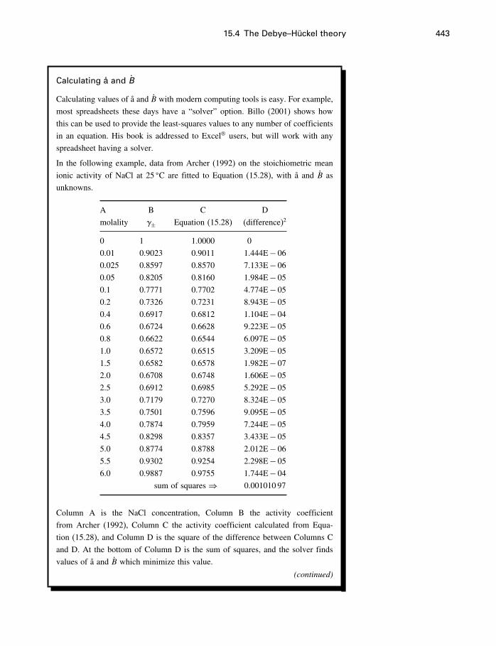
15.4 The Debye–Hückel theory 443
Calculating å and B
Calculating values of å and B with modern computing tools is easy. For example,
most spreadsheets these days have a “solver” option. Billo (2001) shows how
this can be used to provide the least-squares values to any number of coefficients
in an equation. His book is addressed to Excel® users, but will work with any
spreadsheet having a solver.
In the following example, data from Archer (1992) on the stoichiometric mean
ionic activity of NaCl at 25 �C are fitted to Equation (15.28), with å and B as
unknowns.
A B C D
molality ± Equation (15.28) (difference)2
0 1 1.0000 0
0.01 0.9023 0.9011 1.444E− 06
0.025 0.8597 0.8570 7.133E− 06
0.05 0.8205 0.8160 1.984E− 05
0.1 0.7771 0.7702 4.774E− 05
0.2 0.7326 0.7231 8.943E− 05
0.4 0.6917 0.6812 1.104E− 04
0.6 0.6724 0.6628 9.223E− 05
0.8 0.6622 0.6544 6.097E− 05
1.0 0.6572 0.6515 3.209E− 05
1.5 0.6582 0.6578 1.982E− 07
2.0 0.6708 0.6748 1.606E− 05
2.5 0.6912 0.6985 5.292E− 05
3.0 0.7179 0.7270 8.324E− 05
3.5 0.7501 0.7596 9.095E− 05
4.0 0.7874 0.7959 7.244E− 05
4.5 0.8298 0.8357 3.433E− 05
5.0 0.8774 0.8788 2.012E− 06
5.5 0.9302 0.9254 2.298E− 05
6.0 0.9887 0.9755 1.744E− 04
sum of squares ⇒ 0.001010 97
Column A is the NaCl concentration, Column B the activity coefficient
from Archer (1992), Column C the activity coefficient calculated from Equa-
tion (15.28), and Column D is the square of the difference between Columns C
and D. At the bottom of Column D is the sum of squares, and the solver finds
values of å and B which minimize this value.
(continued)
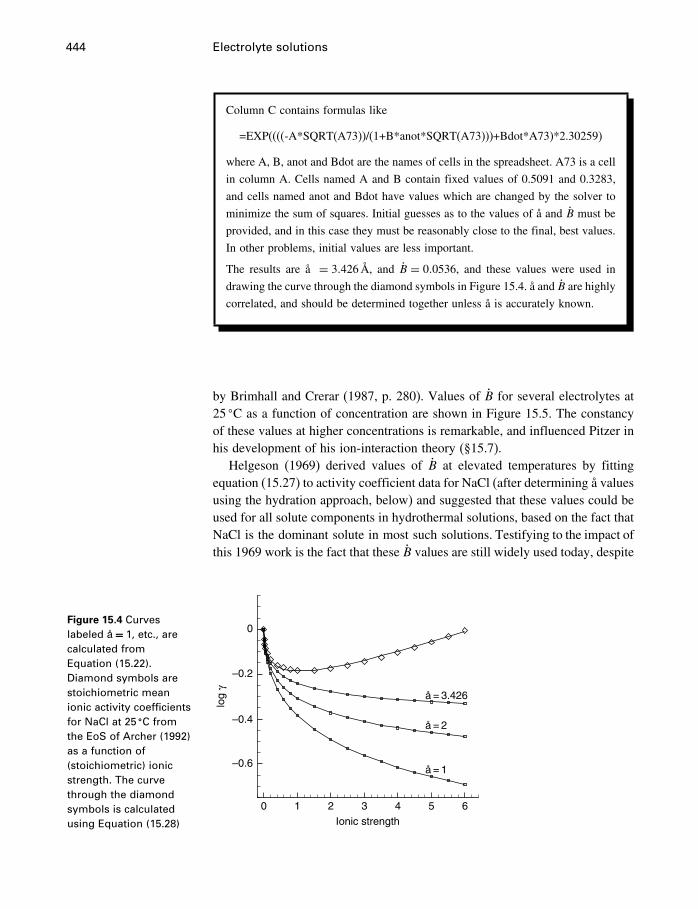
444 Electrolyte solutions
Column C contains formulas like
=EXP((((-A*SQRT(A73))/(1+B*anot*SQRT(A73)))+Bdot*A73)*2.30259)
where A, B, anot and Bdot are the names of cells in the spreadsheet. A73 is a cell
in column A. Cells named A and B contain fixed values of 0.5091 and 0.3283,
and cells named anot and Bdot have values which are changed by the solver to
minimize the sum of squares. Initial guesses as to the values of å and B must be
provided, and in this case they must be reasonably close to the final, best values.
In other problems, initial values are less important.
The results are å = 3�426Å, and B = 0�0536, and these values were used in
drawing the curve through the diamond symbols in Figure 15.4. å and B are highly
correlated, and should be determined together unless å is accurately known.
by Brimhall and Crerar (1987, p. 280). Values of B for several electrolytes at25 �C as a function of concentration are shown in Figure 15.5. The constancyof these values at higher concentrations is remarkable, and influenced Pitzer inhis development of his ion-interaction theory (§15.7).
Helgeson (1969) derived values of B at elevated temperatures by fittingequation (15.27) to activity coefficient data for NaCl (after determining å valuesusing the hydration approach, below) and suggested that these values could beused for all solute components in hydrothermal solutions, based on the fact thatNaCl is the dominant solute in most such solutions. Testifying to the impact ofthis 1969 work is the fact that these B values are still widely used today, despite
Figure 15.4 Curveslabeled å = 1, etc., arecalculated fromEquation (15.22).Diamond symbols arestoichiometric meanionic activity coefficientsfor NaCl at 25 �C fromthe EoS of Archer (1992)as a function of(stoichiometric) ionicstrength. The curvethrough the diamondsymbols is calculatedusing Equation (15.28) Ionic strength
log
γ
0 1 2 3 4 5 6
–0.2
–0.4
–0.6
0
å = 1
å = 2
å = 3.426
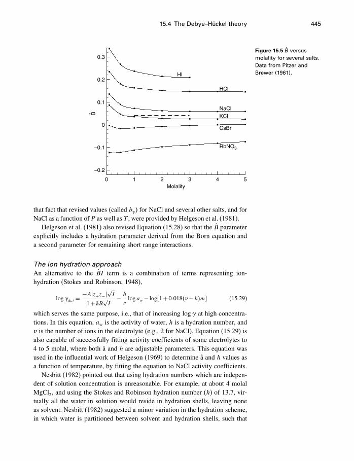
15.4 The Debye–Hückel theory 445
Molality
B°
0 1 2 3 4 5
0.3
0.2
0.1
0
–0.1
–0.2
HI
HCl
NaClKCl
CsBr
RbNO3
Figure 15.5 B versusmolality for several salts.Data from Pitzer andBrewer (1961).
that fact that revised values (called b) for NaCl and several other salts, and forNaCl as a function of P as well as T , were provided by Helgeson et al. (1981).
Helgeson et al. (1981) also revised Equation (15.28) so that the B parameterexplicitly includes a hydration parameter derived from the Born equation anda second parameter for remaining short range interactions.
The ion hydration approachAn alternative to the BI term is a combination of terms representing ion-hydration (Stokes and Robinson, 1948),
log±�i =−A�z+z−�
√I
1+ åB√I
− h�logaw− log�1+0�018��−h�m� (15.29)
which serves the same purpose, i.e., that of increasing log at high concentra-tions. In this equation, aw is the activity of water, h is a hydration number, and� is the number of ions in the electrolyte (e.g., 2 for NaCl). Equation (15.29) isalso capable of successfully fitting activity coefficients of some electrolytes to4 to 5 molal, where both å and h are adjustable parameters. This equation wasused in the influential work of Helgeson (1969) to determine å and h values asa function of temperature, by fitting the equation to NaCl activity coefficients.
Nesbitt (1982) pointed out that using hydration numbers which are indepen-dent of solution concentration is unreasonable. For example, at about 4 molalMgCl2, and using the Stokes and Robinson hydration number (h) of 13.7, vir-tually all the water in solution would reside in hydration shells, leaving noneas solvent. Nesbitt (1982) suggested a minor variation in the hydration scheme,in which water is partitioned between solvent and hydration shells, such that
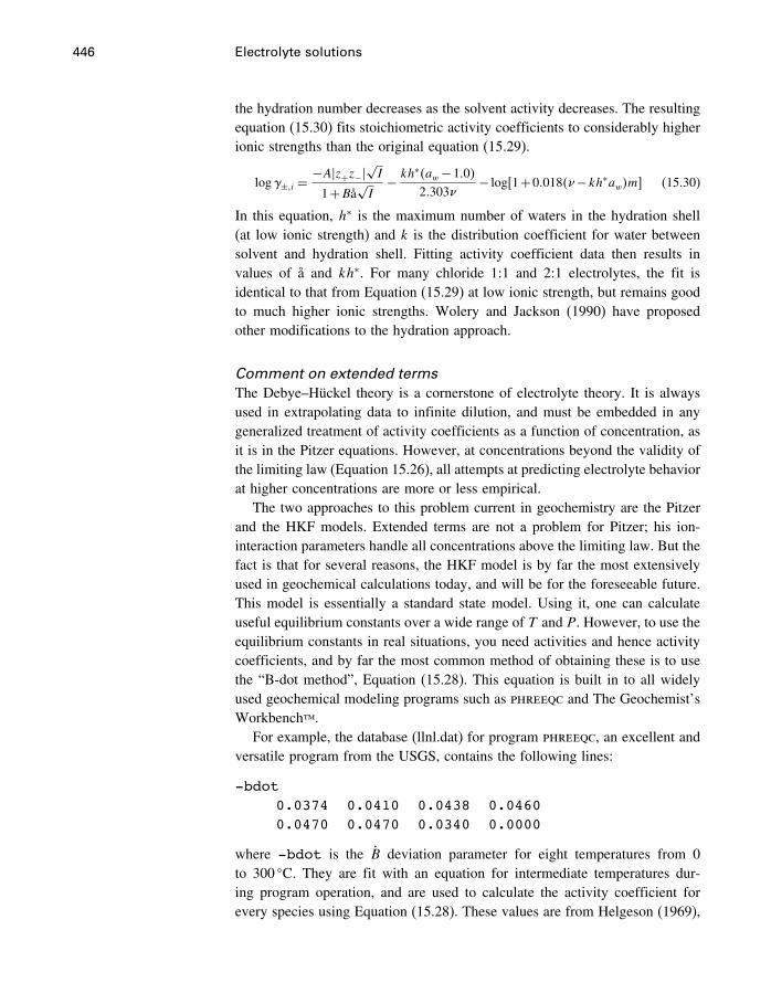
446 Electrolyte solutions
the hydration number decreases as the solvent activity decreases. The resultingequation (15.30) fits stoichiometric activity coefficients to considerably higherionic strengths than the original equation (15.29).
log±�i =−A�z+z−�
√I
1+Bå√I − kh∗�aw−1�0�2�303�
− log�1+0�018��−kh∗aw�m� (15.30)
In this equation, h∗ is the maximum number of waters in the hydration shell(at low ionic strength) and k is the distribution coefficient for water betweensolvent and hydration shell. Fitting activity coefficient data then results invalues of å and kh∗. For many chloride 1:1 and 2:1 electrolytes, the fit isidentical to that from Equation (15.29) at low ionic strength, but remains goodto much higher ionic strengths. Wolery and Jackson (1990) have proposedother modifications to the hydration approach.
Comment on extended termsThe Debye–Hückel theory is a cornerstone of electrolyte theory. It is alwaysused in extrapolating data to infinite dilution, and must be embedded in anygeneralized treatment of activity coefficients as a function of concentration, asit is in the Pitzer equations. However, at concentrations beyond the validity ofthe limiting law (Equation 15.26), all attempts at predicting electrolyte behaviorat higher concentrations are more or less empirical.
The two approaches to this problem current in geochemistry are the Pitzerand the HKF models. Extended terms are not a problem for Pitzer; his ion-interaction parameters handle all concentrations above the limiting law. But thefact is that for several reasons, the HKF model is by far the most extensivelyused in geochemical calculations today, and will be for the foreseeable future.This model is essentially a standard state model. Using it, one can calculateuseful equilibrium constants over a wide range of T and P. However, to use theequilibrium constants in real situations, you need activities and hence activitycoefficients, and by far the most common method of obtaining these is to usethe “B-dot method”, Equation (15.28). This equation is built in to all widelyused geochemical modeling programs such as phreeqc and The Geochemist’sWorkbench™.
For example, the database (llnl.dat) for program phreeqc, an excellent andversatile program from the USGS, contains the following lines:
-bdot0.0374 0.0410 0.0438 0.04600.0470 0.0470 0.0340 0.0000
where -bdot is the B deviation parameter for eight temperatures from 0to 300 �C. They are fit with an equation for intermediate temperatures dur-ing program operation, and are used to calculate the activity coefficient forevery species using Equation (15.28). These values are from Helgeson (1969),
15.5 Activity coefficients of neutral molecules 447
Table 2. The database used by The Geochemist’s Workbench™ has identicalvalues.
The problem with this is that although appropriate values of å and B canfit activity coefficients to high concentration, as shown in Figure 15.4, theymust be determined for individual sets of data. In addition, they are highlycorrelated, so that values of B are very sensitive to changes in å. The databasesmentioned use a single, fixed value of å for each species at all temperatures,obtained from generalized sources such as Kielland (1937). Then there arelesser problems, such as that Helgeson (1969) used “true ionic strength” indetermining B, whereas the å values from most sources were determined usingstoichiometric ionic strength.
What happens to these terms in complex multisalt solutions at high tem-peratures and pressures is generally unknown. But then, many geochemicalcalculations give results for situations in which no one knows what to expect,so errors introduced by activity coefficients go unrecognized. Where compar-isons with experimental data are made, the results can be shockingly bad, asshown in Figure 15.6.
Apart from the problem of lack of data, especially kinetic data, this sit-uation probably constitutes the most serious problem in the application ofthermodynamics to geochemical problems involving hydrothermal solutions.The development of an algorithm which is more accurate than the B-dot methodas presently used, but which could still be used for any species at any T and Pwould be a significant advance in geochemical modeling practice.
15.5 Activity coefficients of neutral molecules
Activity coefficients of electrolytes are determined in a number of ways, but athigher temperatures the problems become more difficult. A pioneering effortwas the direct determination of water activity in NaCl solutions by a high-temperature type of isopiestic apparatus by Liu and Lindsay (1972), and theGibbs–Duhem calculation of NaCl activity coefficients. More recently, high-temperature flow calorimetry determinations of excess enthalpy and heat capac-ity, plus density measurements, are combined to give excess Gibbs energiesand hence activity coefficients.
The determination of the activity coefficients of species that exist dom-inantly as neutral molecules, such as SiO2�aq�, H2S�aq�, and CO2�aq�, ismuch simpler. In these cases it is usually possible to establish a two-phaseequilibrium between the substance in its pure state (solid or gaseous) and thesubstance in its aqueous or dissolved state. This leads to a simple and rigorousdetermination of the activity coefficient in solutions of varying composition.
For example, consider H2S gas in equilibrium with H2S�aq�. The firstionization constant of H2S is about 10−7, so that species other than molecularH2S can be neglected in this connection. The reaction of interest is
H2S�g�= H2S�aq�
448 Electrolyte solutions
for which the equilibrium constant is
K = aH2S�aq�/aH2S�g�
=mH2SH2S
/fH2S
fH2Scan either be taken as equal to the partial pressure of H2S or calculated
from this quantity, and mH2Sis measurable as the total sulfur content of the
solution. Then if K is known, H2Scan be obtained in any solution simply by
measuring fH2Sand mH2S
. For solids such as SiO2 which dissolve to neutralspecies, the situation is even simpler, as the activity of the solid can be takenas 1.0. Normally, K is obtained by performing the experiment in pure water,and assuming that in this case, i = 1. Therefore, activity coefficients obtainedin this way are actually values of
i� in solution of interest, i.e., a salt solution�i� in pure water).
If the “solution of interest” is a solution of neutral salt B in water, havingconcentration mB, eliminating the first term in Equation (15.28) gives
logi = kSmB
where kS replaces B and is called the Setchénow coefficient, andm replaces I . Insome treatments, the I or I term is retained. It is common practice in modelingstudies (e.g., as in virtually all commonly available speciation programs) toassume that the activity coefficient of all uncharged species is 1.0, or to havea single fixed Setchénow coefficient, usually 0.1, which is a common valueat 25 �C. However, measured activity coefficients of aqueous H2S, CO2, SiO2,H3BO3, etc., show a much more complex behavior, being quite different indifferent salt solutions, with positive values in some and negative in others. ThePitzer equations provide a more detailed and accurate treatment of unchargedspecies in the form of measured � coefficients (Equations 15.35–15.39). Bartaand Bradley (1985) derived Pitzer interaction coefficients from the solubility ofH2S, CO2 and CH4 in NaCl solutions from 25 to 350 �C, and 0–6 molal. Thiswas used by Barrett et al. (1988) to derive Setchénow coefficients for thesegases to 300 �C. Also note the completely different approach using regularsolution theory by Nesbitt (§10.6.1).
An extensive review of neutral solutes in aqueous salt solutions is givenby Randell and Failey (1927a, b, c). See also Long and McDevit (1952) andOelkers and Helgeson (1991). Note that we have only spoken of neutral speciesof the type that can be obtained as the dominant species in a solution; activitycoefficients for the neutral species of weak electrolytes and other neutral speciesin a matrix of charged particles constitute a more difficult problem. Theiractivity coefficients are usually assumed to be 1.0, or are taken as equal to those
15.6 Ion association, ion pairs, and complexes 449
of some other neutral species such as H2S or CO2 under the same conditions,without much justification.
The activity coefficients of neutral species in electrolyte solutions at ele-vated temperatures and pressures is a subject of continued study (Oelkers andHelgeson, 1991).
15.6 Ion association, ion pairs, and complexes
Soon after the appearance of the Debye–Hückel theory, it was found that thetheory did not work well for many electrolytes. In 1926, Bjerrum suggestedthat electrostatic attraction between pairs of oppositely charged ions resulted in“ion-pairs,” which would account for the lower measured activity coefficientsin these solutions. The problem then, as now, was how best to define andmeasure the extent of ion-pairing. How close must two ions be to become anion-pair? What is the difference between an ion-pair and a complex? Is it reallynecessary to know this to use thermodynamics? Helgeson (1981) notes that“The distinction between ion association and short-range ionic interaction isnebulous at best.”
A simple view is that in an ion-pair the two ions are separated by one or morewater molecules, while in a complex the ions are in contact, often covalentlybonded. However, the distinction is not easily made, and there appear to be allgradations between the two. One common distinction, however, is that at highertemperatures, there is an increase in ion-pairing, but a decrease in complexformation. The reason for increased ion-pairing is due mainly to the decreasein the dielectric constant of water, as discussed in §6.2.4, and the decrease incomplexing is due to the increased thermal energy of the particles, tending tobreak them apart.
The decrease in dielectric constant of water, resulting in increased electro-static attraction between oppositely charged ions, means that many “strong”electrolytes become “weak” at high temperatures, and the identification ofsolute species becomes easier, or even possible, by various spectroscopic meth-ods. That is, there are sufficient particles, and they stay together long enough,to produce absorption of radiation. This difference between solutions at roomtemperature and those at high temperature results in a corresponding differencein opinions about how best to think about them.
For most electrolyte solutions at or near room temperature, there havebeen two main approaches, exemplified by the Pitzer and HKF models to bedescribed below. (These two approaches were also mentioned on page 304.) Inone, referred to as ion-interaction theory and embodied in the Pitzer equations,no attempt is made (except if there are very strong complexes present) to iden-tify species. Components are treated stoichiometrically, and all ion interactionsare accounted for in the form of fit coefficients in some form of equation.Advocates of this approach point to the rather uncertain nature of our knowl-edge of aqueous species. Molecular dynamics simulations of these solutions
450 Electrolyte solutions
(e.g., Driesner et al, 1998) show that the “real” situation is probably verycomplicated. So the answer to one question is no, you do not have to knowanything about what is happening in the solution to use thermodynamics. Inthe other approach, called ion-association, and embodied in the HKF modeland program supcrt92, ion-pair and complex species are identified and theiractivities calculated using activity coefficients calculated from D–H theory.The fact that such species become more abundant and more easily measuredat high temperature therefore has an effect on one’s thinking about how toapproach this problem.
Pitzer, in a discussion following Helgeson’s (1981) paper outlining the HKFmodel, put the situation clearly. The “alternative competitive formulations”referred to are the two approaches mentioned above.
As I see it, the domain in which alternative competitive formulations are
more-or-less equally effective is roughly the region of water density greater
than 0.7 to 0.8. Clearly, when you get water densities much less than 0.7,
you’re going into the domain where strong electrolytes become weak
electrolytes. I fully understand Dr. Helgeson’s reasons for wanting to maintain a
single type of treatment continuously across that boundary. On the other hand,
there are advantages, if you’re working primarily in this relatively high
dielectric – high density domain, of dealing with the materials as if they were
completely dissociated. Again, I emphasize that the amount of dissociation in
that territory is at least somewhat arbitrary.
This pretty well sums up the present situation. In problem areas dealingwith concentrated solutions at or near the Earth’s surface, that is, in thehigh dielectric constant, high density domain, the ion-interaction or Pitzerequation approach is dominant. In problem areas dealing with hydrother-mal, metamorphic or aqueous solutions of igneous origin, the ion-pairing,species identification approach is dominant, and at the moment the HKFmodel is the most widely used. Each approach is weak in the other’s domain.Pitzer equations do not yet have many parameters available for high temper-atures and pressures, and although ion-pairing and B-dot activity coefficientscan be used for concentrated, low temperature solutions, the results can bedisastrous (Figure 15.6).
It is interesting to note that considerations of ion-pairs versus complexesare problems in physical chemistry, not in thermodynamics. Whether there areion-pairs or complexes, one uses the available data on equilibrium constantsor ion-interaction constants and makes the necessary calculations. In fact,in many geochemical discussions, no distinction is made between ion-pairsand complexes. All species are commonly referred to as complexes – if anequilibrium constant or an ion-interaction constant is available, it doesn’t matterwhat it is called.
15.7 The Pitzer equations 451
15.7 The Pitzer equations
In the 1970s, Kenneth Pitzer and his associates developed a theoretical modelfor the excess Gibbs energy of electrolyte solutions which combines the Debye–Hückel equation with additional terms in the form of a virial equation. This hasproven to be extraordinarily successful at fitting the behavior of both single-and mixed-salt solutions to high concentrations. Summary articles outlining thisapproach, with references to the primary sources, are Pitzer (1981, 1987, 1991),and Pitzer (1995) presents a comprehensive treatment of thermodynamics whichintegrates this approach with other subjects.
Much of the theory underlying the Pitzer equations was developed forgases and extended to electrolyte solutions largely by Joseph Mayer (Mayerand Mayer, 1940; Mayer, 1950), and especially McMillan and Mayer (1945).For a brief summary see McQuarrie (2000, Chapter 15) and for a compre-hensive summary see Friedman, (1962). If you do consult these references,your knowledge of statistical mechanics had better be pretty good. Mazo andMou (1991) describe the technical details in McMillan and Mayer as “ratherintricate.”
The model relates the excess total Gibbs energy of a system to an equationsimilar in principle to the virial equation we saw for gases in §13.5, in whichthe first term is not the ideal gas expression, but a simplified form of theDebye–Hückel equation. The general equation used by Pitzer (from whichmany others are derived by differentiation) is
Gex
kgwRT= f�I�+∑
i
∑j
�ij mimj+∑i
∑j
∑k
�ijk mimjmk (15.31)
where kgw is the number of kilograms of water. This means we consider thetotal Gibbs energy of a system containing 1 kg of water, which in turn meansall concentration will be molalities. Gex/kgw is not the same as Gex.
The first virial coefficient f�I� is some function of the ionic strengthand is not 0 as it would be for an ideal solution, but is in fact a ver-sion of the Debye–Hückel equation, which represents departure from idealityin very dilute solutions. The following term is a function of the interac-tions of all pairs of ions, and the third term a function of the interactionsof ions taken three at a time. The second coefficient, �ij , is a function ofionic strength, but the third coefficient �ijk is considered to be independentof ionic strength and equals zero if i, j, and k are all anions or cations.Later extensions to the model published by Pitzer and co-workers allowfor an ionic strength dependence to the third coefficient. Pitzer (1987) andHarvie and Weare (1980) note that higher virial coefficients are required onlyfor extremely concentrated solutions, so the series is stopped at the thirdcoefficient.
452 Electrolyte solutions
To relate this to activity coefficients we know, from (10.53) and (10.54),that the partial derivatives of Gex in (15.31) are(
�Gex/�kgwRT��mi
)P�T�nH2O
= �exi /RT
= lni
and
�−1=− ��Gex/�kgw�niRT∑i mi
Equation (15.31) can therefore be rewritten in terms of activity coefficientsfor specific ions and the osmotic coefficient of the solvent by forming theappropriate derivatives of the virial terms on the right hand side. The finalform taken by these terms was a subject of both theoretical considerations andempirical trial-and-error, and is described in Pitzer (1973). Omitting a greatdeal of such development, the final working equations are as follows, usingthe notation of Harvie et al. (1984).
The equations for a binary electrolyte solution are relatively simple. Formixed electrolytes they get a bit more complicated. We look first at the equa-tions for a binary electrolyte.
15.7.1 Binary electrolytes MX
First, the parametric equation for excess Gibbs energy is
Gex
kgwRT=−A�
(4Ib
)ln�1+b√I�
+2�M�X[m2BMX+m3�MzMCMX
] (15.32)
where
BMX = ��0�+2��1�MX[1− �1+√I� exp�−√I�
]/2I
CMX = C�MX/2√�zMzX�
The corresponding equations for the osmotic and activity coefficients are
Osmotic coefficient
�−1=−�zMzX�A�√I
1+b√I+m2�M�X
�
[��0�MX+��1�MX exp�−
√I�]
(15.33)
+m2 2��M�X�3/2
�C�MX
15.7 The Pitzer equations 453
In these equations, � = �M + �X , where � is the number of ions; z is thecharge on the ion, I is the (stoichiometric) molal ionic strength, and other termsare explained below.
Stoichiometric mean ionic activity coefficient
ln± = −�zMzX�A�[ √
I
1+b√I +2bln�1+b√I�
]
+m2�M�X�
{2��0�MX+
2��1�MX2I
[1−(1+√I−
2I
2
)exp�−√I�
]}
+ 3m2
2
[2��M�X�
3/2
�C�MX
](15.34)
15.7.2 Mixed electrolytes
Osmotic coefficient
�−1= 2∑i mi
[−A�I3/21+bI1/2 +
Nc∑c=1
Na∑a=1
mcma�B�ca+ZCca�
+Nc−1∑c=1
Nc∑c′=c+1
mcmc′
(��cc′ +
Na∑a=1
ma cc′a
)
+Na−1∑a=1
Na∑a′=a+1
mama′
(��aa′ +
Nc∑c=1
mc aa′c
)
+Nn∑n=1
Na∑a=1
mnma�na+Nn∑n=1
nc∑c=1
mnmc�nc
](15.35)
The activity coefficient for water is then
lnaH2O=−18�0154
1000
(Nc+Na∑i
mi
)� (15.36)
Activity coefficient for cation X
lnX = z2XF +Nc∑c=1
mc�2BcX+ZCcX�+Na∑a=1
ma
(2�Xa+
Nc∑c=1
mc Xac
)
+Nc−1∑c=1
Nc∑c′=c+1
mcmc′ cc′X+�zX�Nc∑c=1
Na∑a=1
mcmaCca+Nn∑n=1
mn�2�nX�
(15.37)
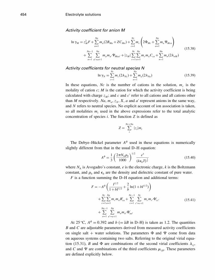
454 Electrolyte solutions
Activity coefficient for anion M
lnM = z2MF +Na∑a=1
ma�2BMa+ZCMa�+Nc∑c=1
mc
(2�Mc+
Na∑a=1
ma Mca
)
+Na−1∑a=1
Na∑a′=a+1
mama′ Maa′ + �zM �Nc∑c=1
Na∑a=1
mcmaCca+Nn∑n=1
mn�2�nM�
(15.38)
Activity coefficients for neutral species N
lnN =Nc∑c=1
mc�2�Nc�+Na∑a=1
ma�2�Na� (15.39)
In these equations, Nc is the number of cations in the solution, mc is themolality of cation c; M is the cation for which the activity coefficient is beingcalculated with charge zM ; and c and c
′ refer to all cations and all cations otherthanM respectively. Na, ma, zX , X, a and a
′ represent anions in the same way,and N refers to neutral species. No explicit account of ion association is taken,so all molalities mi used in the above expressions refer to the total analyticconcentration of species i. The function Z is defined as
Z =Nc+Na∑i
�zi�mi
The Debye–Hückel parameter A� used in these equations is numericallyslightly different from that in the usual D–H equation:
A� = 13
(2!NA�01000
)1/2e3
�k�0T�32
(15.40)
where NA is Avogadro’s constant, e is the electronic charge, k is the Boltzmannconstant, and �0 and �0 are the density and dielectric constant of pure water.F is a function summing the D–H equation and additional terms:
F =−A�(
I1/2
1+bI1/2 +2bln�1+bI1/2�
)
+Nc∑c=1
Na∑a=1
mcmaB′ca+
Nc−1∑c=1
Nc∑c′=c+1
mcmc′�′cc′
+Na−1∑a=1
Na∑a′=a+1
mama′�′aa′
(15.41)
At 25 �C, A� = 0�392 and b (= åB in D–H) is taken as 1.2. The quantitiesB and C are adjustable parameters derived from measured activity coefficientson single salt + water solutions. The parameters � and come from dataon aqueous systems containing two salts. Referring to the original virial equa-tion (15.31), B and � are combinations of the second virial coefficients �ij ,and C and are combinations of the third coefficients �ijk. These parametersare defined explicitly below.
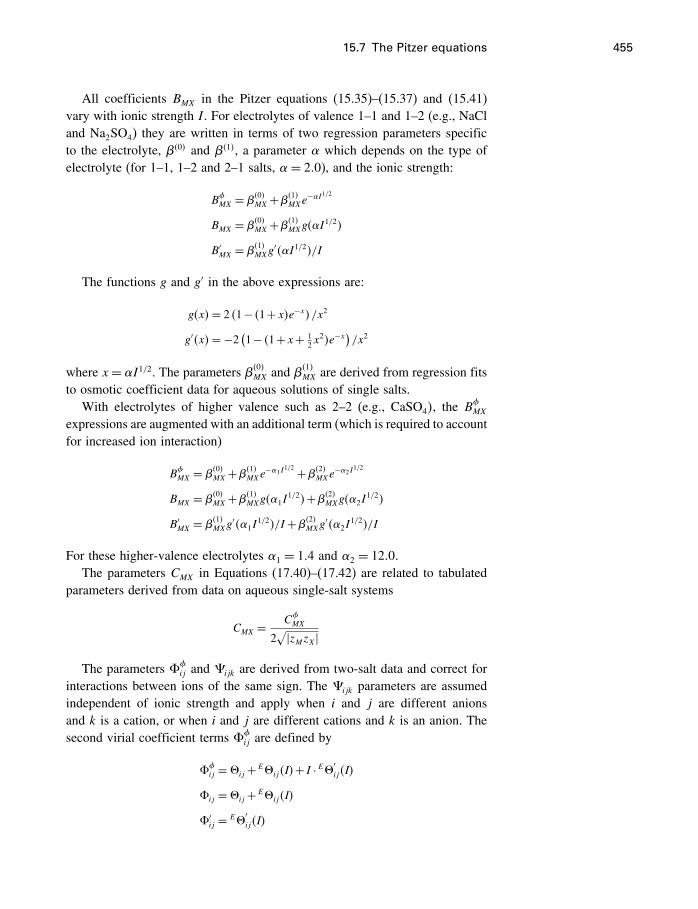
15.7 The Pitzer equations 455
All coefficients BMX in the Pitzer equations (15.35)–(15.37) and (15.41)vary with ionic strength I . For electrolytes of valence 1–1 and 1–2 (e.g., NaCland Na2SO4) they are written in terms of two regression parameters specificto the electrolyte, ��0� and ��1�, a parameter which depends on the type ofelectrolyte (for 1–1, 1–2 and 2–1 salts, = 2�0), and the ionic strength:
B�MX = ��0�MX+��1�MXe−I1/2
BMX = ��0�MX+��1�MXg�I1/2�B′MX = ��1�MXg′�I1/2�/I
The functions g and g′ in the above expressions are:
g�x�= 2 �1− �1+x�e−x� /x2
g′�x�=−2(1− �1+x+ 1
2x2�e−x
)/x2
where x= I1/2. The parameters ��0�MX and ��1�MX are derived from regression fitsto osmotic coefficient data for aqueous solutions of single salts.
With electrolytes of higher valence such as 2–2 (e.g., CaSO4�, the B�MX
expressions are augmented with an additional term (which is required to accountfor increased ion interaction)
B�MX = ��0�MX+��1�MXe−1I1/2 +��2�MXe−2I1/2
BMX = ��0�MX+��1�MXg�1I1/2�+��2�MXg�2I
1/2�
B′MX = ��1�MXg′�1I
1/2�/I+��2�MXg′�2I1/2�/I
For these higher-valence electrolytes 1 = 1�4 and 2 = 12�0�The parameters CMX in Equations (17.40)–(17.42) are related to tabulated
parameters derived from data on aqueous single-salt systems
CMX = C�MX
2√�zMzX�
The parameters ��ij and ijk are derived from two-salt data and correct forinteractions between ions of the same sign. The ijk parameters are assumedindependent of ionic strength and apply when i and j are different anionsand k is a cation, or when i and j are different cations and k is an anion. Thesecond virial coefficient terms ��ij are defined by
��ij ="ij+ E"ij�I�+ I · E"′
ij�I�
�ij ="ij+ E"ij�I�
�′ij = E"
′ij�I�
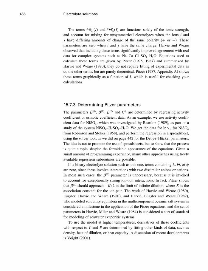
456 Electrolyte solutions
The terms E"ij�I� andE"′
ij�I� are functions solely of the ionic strength,and account for mixing for unsymmetrical electrolytes when the ions i andj have differing amounts of charge of the same polarity (+ or −). Theseparameters are zero when i and j have the same charge. Harvie and Weareobserved that including these terms significantly improved agreement with realdata for complex systems such as Na–Ca–Cl–SO4–H2O. Equations used tocalculate these terms are given by Pitzer (1975, 1987) and summarized byHarvie and Weare (1980); they do not require fitting of experimental data asdo the other terms, but are purely theoretical. Pitzer (1987, Appendix A) showsthese terms graphically as a function of I , which is useful for checking yourcalculations.
15.7.3 Determining Pitzer parameters
The parameters ��0�, ��1�, ��2� and C� are determined by regressing activitycoefficient or osmotic coefficient data. As an example, we use activity coeffi-cient data for NiSO4, which was investigated by Reardon (1989), as part of astudy of the system NiSO4–H2SO4–H2O. We get the data for ln± for NiSO4
from Robinson and Stokes (1958), and perform the regression in a spreadsheet,using the solver tool, as we did on page 442 for the Debye–Hückel parameters.The idea is not to promote the use of spreadsheets, but to show that the processis quite simple, despite the formidable appearance of the equations. Given asmall amount of programming experience, many other approaches using freelyavailable regression subroutines are possible.
In a binary electrolyte solution such as this one, terms containing �, ", or �are zero, since these involve interactions with two dissimilar anions or cations.In most such cases, the ��2� parameter is unnecessary, because it is invokedto account for exceptionally strong ion–ion interactions. In fact, Pitzer showsthat ��2� should approach −K/2 in the limit of infinite dilution, where K is theassociation constant for the ion-pair. The work of Harvie and Weare (1980),Eugster, Harvie and Weare (1980), and Harvie, Eugster and Weare (1982),who modeled solubility equilibria in the multicomponent oceanic salt system isconsidered a milestone in the application of the Pitzer equations, and the set ofparameters in Harvie, Mller and Weare (1984) is considered a sort of standardfor modeling of seawater evaporitic systems.
To use the model at higher temperatures, derivatives of these coefficientswith respect to T and P are determined by fitting other kinds of data, such asdensity, heat of dilution, or heat capacity. A discussion of recent developmentsis Voight (2001).
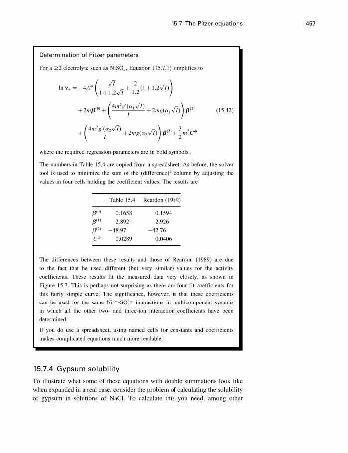
15.7 The Pitzer equations 457
Determination of Pitzer parameters
For a 2:2 electrolyte such as NiSO4, Equation (15.7.1) simplifies to
ln± = −4A�( √
I
1+1�2√I+ 2
1�2�1+1�2
√I�
)
+2m��0�+(4m2g′�1
√I�
I+2mg�1
√I�
)��1�
+(4m2g′�2
√I�
I+2mg�2
√I�
)��2�+ 3
2m2C�
(15.42)
where the required regression parameters are in bold symbols.
The numbers in Table 15.4 are copied from a spreadsheet. As before, the solver
tool is used to minimize the sum of the �difference�2 column by adjusting the
values in four cells holding the coefficient values. The results are
Table 15.4 Reardon (1989)
��0� 0�1658 0�1594
��1� 2�892 2�926
��2� −48�97 −42�76
C� 0�0289 0�0406
The differences between these results and those of Reardon (1989) are due
to the fact that he used different (but very similar) values for the activity
coefficients. These results fit the measured data very closely, as shown in
Figure 15.7. This is perhaps not surprising as there are four fit coefficients for
this fairly simple curve. The significance, however, is that these coefficients
can be used for the same Ni2+-SO2−4 interactions in multicomponent systems
in which all the other two- and three-ion interaction coefficients have been
determined.
If you do use a spreadsheet, using named cells for constants and coefficients
makes complicated equations much more readable.
15.7.4 Gypsum solubility
To illustrate what some of these equations with double summations look likewhen expanded in a real case, consider the problem of calculating the solubilityof gypsum in solutions of NaCl. To calculate this you need, among other
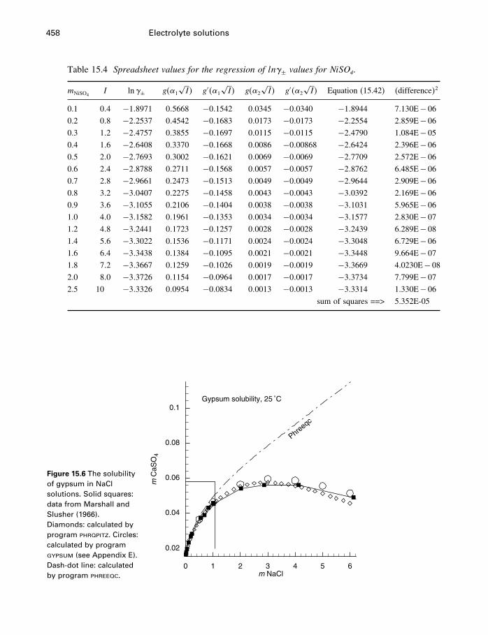
458 Electrolyte solutions
Table 15.4 Spreadsheet values for the regression of ln± values for NiSO4.
mNiSO4I ln± g�1
√I� g′�1
√I� g�2
√I� g′�2
√I� Equation (15.42) �difference�2
0.1 0�4 −1�8971 0�5668 −0�1542 0�0345 −0�0340 −1�8944 7.130E− 06
0.2 0�8 −2�2537 0�4542 −0�1683 0�0173 −0�0173 −2�2554 2.859E− 06
0.3 1�2 −2�4757 0�3855 −0�1697 0�0115 −0�0115 −2�4790 1.084E− 05
0.4 1�6 −2�6408 0�3370 −0�1668 0�0086 −0�00868 −2�6424 2.396E− 06
0.5 2�0 −2�7693 0�3002 −0�1621 0�0069 −0�0069 −2�7709 2.572E− 06
0.6 2�4 −2�8788 0�2711 −0�1568 0�0057 −0�0057 −2�8762 6.485E− 06
0.7 2�8 −2�9661 0�2473 −0�1513 0�0049 −0�0049 −2�9644 2.909E− 06
0.8 3�2 −3�0407 0�2275 −0�1458 0�0043 −0�0043 −3�0392 2.169E− 06
0.9 3�6 −3�1055 0�2106 −0�1404 0�0038 −0�0038 −3�1031 5.965E− 06
1.0 4�0 −3�1582 0�1961 −0�1353 0�0034 −0�0034 −3�1577 2.830E− 07
1.2 4�8 −3�2441 0�1723 −0�1257 0�0028 −0�0028 −3�2439 6.289E− 08
1.4 5�6 −3�3022 0�1536 −0�1171 0�0024 −0�0024 −3�3048 6.729E− 06
1.6 6�4 −3�3438 0�1384 −0�1095 0�0021 −0�0021 −3�3448 9.664E− 07
1.8 7�2 −3�3667 0�1259 −0�1026 0�0019 −0�0019 −3�3669 4.0230E− 08
2.0 8�0 −3�3726 0�1154 −0�0964 0�0017 −0�0017 −3�3734 7.799E− 07
2.5 10 −3�3326 0�0954 −0�0834 0�0013 −0�0013 −3�3314 1.330E− 06
sum of squares ==> 5.352E-05
Figure 15.6 The solubilityof gypsum in NaClsolutions. Solid squares:data from Marshall andSlusher (1966).Diamonds: calculated byprogram phrqpitz. Circles:calculated by programgypsum (see Appendix E).Dash-dot line: calculatedby program phreeqc. m NaCl
m C
aSO
4
0 1 2 3 4 5 6
0.02
0.04
0.06
0.08
0.1Gypsum solubility, 25 ˚C
Phreeqc
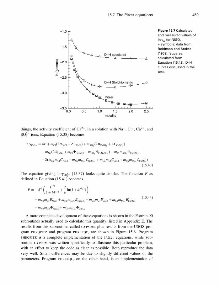
15.7 The Pitzer equations 459
+
+
+
++
++
++
++
+ + ++ + +
molality
ln (
gam
ma)
0.0 0.5 1.0 1.5 2.0 2.5–3.5
–3.0
–2.5
–2.0
–1.5
–1.0
D–H speciated
D–H Stoichiometric
Pitzer
Figure 15.7 Calculatedand measured values ofln�± for NiSO4.+ symbols: data fromRobinson and Stokes(1959). Squares:calculated fromEquation (15.42). D–Hcurves discussed in thetext.
things, the activity coefficient of Ca2+. In a solution with Na+, Cl−, Ca2+, andSO2−
4 ions, Equation (15.38) becomes
lnCa2+ = 4F +mCl�2BCaCl+ZCCaCl�+mSO4�2BCaSO4
+ZCCaSO4�
+mNa�2�CaNa +mCl CaNaCl+mSO4 CaNaSO4
�+mClmSO4 CaClSO4
+2�mNamClCNaCl+mNamSO4CNaSO4
+mCamClCCaCl+mCamSO4CCaSO4
�
(15.43)
The equation giving lnSO2−4
(15.37) looks quite similar. The function F asdefined in Equation (15.41) becomes
F =−A�(
I1/2
1+bI1/2 +2bln�1+bI1/2�
)+mNamClB
′NaCl+mNamSO4
B′NaSO4
+mCamClB′CaCl+mCamSO4
B′CaSO4
+mNamCa�′NaCa +mClmSO4
�′ClSO4
(15.44)
A more complete development of these equations is shown in the Fortran 90subroutines actually used to calculate this quantity, listed in Appendix E. Theresults from this subroutine, called gypsum, plus results from the USGS pro-gram phrqpitz and program phreeqc, are shown in Figure 15.6. Programphrqpitz is a complete implementation of the Pitzer equations, while sub-routine gypsum was written specifically to illustrate this particular problem,with an effort to keep the code as clear as possible. Both reproduce the datavery well. Small differences may be due to slightly different values of theparameters. Program phreeqc, on the other hand, is an implementation of
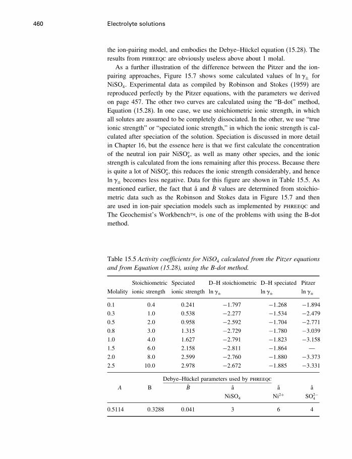
460 Electrolyte solutions
the ion-pairing model, and embodies the Debye–Hückel equation (15.28). Theresults from phreeqc are obviously useless above about 1 molal.
As a further illustration of the difference between the Pitzer and the ion-pairing approaches, Figure 15.7 shows some calculated values of ln± forNiSO4. Experimental data as compiled by Robinson and Stokes (1959) arereproduced perfectly by the Pitzer equations, with the parameters we derivedon page 457. The other two curves are calculated using the “B-dot” method,Equation (15.28). In one case, we use stoichiometric ionic strength, in whichall solutes are assumed to be completely dissociated. In the other, we use “trueionic strength” or “speciated ionic strength,” in which the ionic strength is cal-culated after speciation of the solution. Speciation is discussed in more detailin Chapter 16, but the essence here is that we first calculate the concentrationof the neutral ion pair NiSO�
4, as well as many other species, and the ionicstrength is calculated from the ions remaining after this process. Because thereis quite a lot of NiSO�
4, this reduces the ionic strength considerably, and henceln± becomes less negative. Data for this figure are shown in Table 15.5. Asmentioned earlier, the fact that å and B values are determined from stoichio-metric data such as the Robinson and Stokes data in Figure 15.7 and thenare used in ion-pair speciation models such as implemented by phreeqc andThe Geochemist’s Workbench™, is one of the problems with using the B-dotmethod.
Table 15.5 Activity coefficients for NiSO4 calculated from the Pitzer equationsand from Equation (15.28), using the B-dot method.
Stoichiometric Speciated D–H stoichiometric D–H speciated Pitzer
Molality ionic strength ionic strength ln± ln± ln±
0.1 0�4 0�241 −1�797 −1�268 −1�894
0.3 1�0 0�538 −2�277 −1�534 −2�479
0.5 2�0 0�958 −2�592 −1�704 −2�771
0.8 3�0 1�315 −2�729 −1�780 −3�039
1.0 4�0 1�627 −2�791 −1�823 −3�158
1.5 6�0 2�158 −2�811 −1�864 —
2.0 8�0 2�599 −2�760 −1�880 −3�373
2.5 10�0 2�978 −2�672 −1�885 −3�331
Debye–Hückel parameters used by phreeqc
A B B å å å
NiSO4 Ni2+ SO2−4
0.5114 0�3288 0�041 3 6 4
15.8 The HKF model for aqueous electrolytes 461
15.8 The HKF model for aqueous electrolytes
The other major contribution to the systematization of our knowledge of aque-ous electrolyte solutions at elevated temperatures and pressures takes a com-pletely different approach. This was presented in a series of four papers by H.C.Helgeson and co-workers between 1974 and 1981, with fairly extensive modi-fications added by Tanger and Helgeson (1988). We present here an outline ofthis model, with some explanation and comparison with the Pitzer model. Werefer to it as the HKF or revised HKF model, after the three authors of Part IVof the series of papers just mentioned, Helgeson, Kirkham, and Flowers.
15.8.1 Overall structure of the HKF model
The HKF model is semiempirical, in the sense that it uses a number of empir-ical parameters within a framework suggested by fundamental physics andthermodynamics. The variation of the Gibbs energy of individual ions with T ,P, and composition can be represented by writing the total differential of the(partial molar) Gibbs energy of the jth ion, giving
dGj =−SjdT +V jdP+(��j
�dnj
)T�P
dnj
where j is an ion in an aqueous solution of any composition. Changes in Gjdue to changes in T�P or nj are found by integrating this equation,
∫ T�P�n
Tr �Pr �n0dGj =−
∫ T
TrSj�Pr �n0
dT +∫ P
Pr
V j�T�n0dP+∫ n
n0
d�j�T�P (15.45)
This is illustrated in Figure 15.8. The first two integrals on the right handside take place at concentration n0. If we equate this with the standard state(ideal one molal solution), then Sj and V j become S
�j and V
�j respectively. The
third integral takes care of departures from standard state conditions (change ofcomposition) at T and P. Integration of
∫ TTrS�j dT requires knowledge of CP
�j ,
and integration of∫ nn0d�j (= �j−��
j = RT lnaj) requires knowledge of j , sothat the minimum information needed to know how the Gibbs energy of an ionj varies with T , P, and composition is how CP
�j and V
�j vary with T and P
respectively, and how j varies with composition.
15.8.2 The Born functions
The Born function was introduced in §6.2.4. It is qualitatively accurate butquantitatively inaccurate. However the fact that it succeeds as well as it doessuggests that it contains a large part of the truth, and might serve as the basis ofa more satisfactory model. In fact it serves as the basis of the HKF model, whichuses the Born function to provide the Gibbs energy of solvation (or hydration in
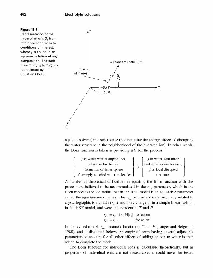
462 Electrolyte solutions
Figure 15.8Representation of theintegration of dGj fromreference conditions toconditions of interest,where j is an ion in anaqueous solution of anycomposition. The pathfrom Tr� Pr�n0 to T�P�n isrepresented byEquation (15.45).
+ Standard State T, P
∫–Sd T
∫VdP∫d
µ
Tr , Pr , no
T
P
nj
T, P, nof interest
+
aqueous solvent) in a strict sense (not including the energy effects of disruptingthe water structure in the neighborhood of the hydrated ion). In other words,the Born function is taken as providing �G for the process⎧⎪⎪⎪⎨⎪⎪⎪⎩
j in water with disrupted local
structure but before
formation of inner sphere
of strongly attached water molecules
⎫⎪⎪⎪⎬⎪⎪⎪⎭→
⎧⎪⎪⎪⎨⎪⎪⎪⎩j in water with inner
hydration sphere formed�
plus local disrupted
structure
⎫⎪⎪⎪⎬⎪⎪⎪⎭A number of theoretical difficulties in equating the Born function with thisprocess are believed to be accommodated in the re�j parameter, which in theBorn model is the ion radius, but in the HKF model is an adjustable parametercalled the effective ionic radius. The re�j parameters were originally related tocrystallographic ionic radii �rx�j� and ionic charge zj in a simple linear fashionin the HKF model, and were independent of T and P
re�j = rx�j+0�94�zj � for cations
re�j = rx�j for anions
In the revised model, re�j became a function of T and P (Tanger and Helgeson,1988), and is discussed below. An empirical term having several adjustableparameters to account for all other effects of adding an ion to water is thenadded to complete the model.
The Born function for individual ions is calculable theoretically, but asproperties of individual ions are not measurable, it could never be tested
15.8 The HKF model for aqueous electrolytes 463
experimentally. Two conventions are required to get around this problem.First, the properties of anions are taken to be equivalent to those of theircorresponding acids, so that for instance the properties of Cl− are equivalentto those of HCl�aq�. Therefore we define a “conventional” electrostatic Bornparameter as
�j =NA�zje�
2
2re�j−(NA�zH+e�2
2re�H+
)· zj
= NA�zje�2
2re�j−0�5387zj (15.46)
where 0.5387 is the value of �NA�zje�2�/�2re�j� for the H+ ion (Helgeson and
Kirkham, 1976). The Born function then becomes
�G�s�j = �j
(1�−1)
(15.47)
which is the difference between the �G of solvation of ion j (j in vacuum → j
in water) and the �G of solvation of H+ (H+ in vacuum → H+ in water). Asdescribed above, in the HKF model, this is equated with the �G of formation ofthe inner hydration sphere only. This is sometimes called the conventional �Gof solvation, although since it is the only one we can deal with in a practicalway, it is more often just called the �G of solvation.
The second convention required is that the properties of individual ions arerelated to the properties of electrolytes by the additivity rule
��k =
∑j
�j�k��j (15.48)
where � is any partial molar property and �j�k represents the stoichiometry ofthe jth ion in the kth electrolyte. An example would be V
�CaCl2
= V �Ca2+ +2V
�Cl− .
Thus for example, because the properties ��� of the Cl− ion are identified withthose of HCl they are “known,” and � for the Ca2+ ion is then obtained from
�Ca2+ =�CaCl2−2�Cl−
In summary, because properties are additive, and the properties of anions areknown by convention, then all ionic properties are knowable, in the conven-tional sense.
It follows from the additivity convention that we can write an analogousBorn function for aqueous electrolytes, k, as
�G�s�k = �k
(1�−1)
where
�k =∑j
�j�k�j
464 Electrolyte solutions
In other words, �k for electrolytes is simply the sum of its �j terms, e.g.,
�CaCl2= �Ca2+ +2�Cl−
(Note that in this summation, the properties of the hydrogen ion cancel out.)It follows too that the fit parameters in the model to be described are alsoadditive, so that the procedure is to develop the fit parameters for data onelectrolytes, then to split them into additive parameters for individual ions. Inthe following equations, if there is no j or k subscript, the equation applies toboth, as long as the appropriate parameters are used.
15.8.3 The re�j term
The (conventional) entropy and volume changes of solvation according to theBorn model are then derived by differentiation, which in the original HKFmodel was a simple procedure because re�j was independent of T�P, whichmeant that �j was also independent of T�P. Thus in the original model,
�S�s =−
(��G
�s
�T
)
=−� �
�T
(1�−1)
(15.49)
= �Y
and
�V�s =
(��G
�s
�P
)
= � �
�P
(1�−1)
(15.50)
=−�Q
and
�CP�s = T
(��S
�s
�T
)
= �T �Y�T
(15.51)
= �TX
where Y , Q, and X are Born coefficients, i.e., temperature and pressure deriva-tives of the dielectric constant of water, derived and calculated by Helgesonand Kirkham (1974a). However, in the revised model, re�j becomes a rather
15.8 The HKF model for aqueous electrolytes 465
complex function of T and P, giving rather more complex expressions forthe solvation terms, containing partial derivatives of �j . It is helpful in seeingthe overall structure of this model to look first at the simple forms of thesolvation contributions (above), and then to regard the more complex forms asunfortunate complications.
In the revised model,
re�j = rx�j+�zj ��0�94+g� for cations
re�j = rx�j+�zj �g for anions
}(15.52)
where, as before, zj is the ionic charge and rx�j is the crystallographic ionicradius. The added term g is a complex function of T and P obtained byregression of volume and heat capacity data for aqueous NaCl. This results ofcourse in more complex expressions for the solvation terms, which are (Tangerand Helgeson 1988, Appendix G)
�S�s =−
(��G
�s
�T
)P
= �Y −(1�−1)(
��
�T
)P
(15.53)
�V�s =
(��G
�s
�P
)T
=−�Q+(1�−1)(
��
�P
)T
(15.54)
and
�CP�s = T
(��S
�s
pT
)
= �TX+2TY(��
�T
)P
−T(1�−1)(
�2�
�T 2
)P
(15.55)
Note that in regions where g= 0 (essentially where T< 150 �C or P> 2000bars), the T and P derivatives of � in these expressions become zero (becausere�j is independent of T�P when g = 0), and the solvation terms resume theiroriginal fairly simple forms.
The re�j term in the HKF model essentially takes the place of the å termin the D–H model, and because it is different for each ion, the overall modelsuffers from the problem mentioned in §15.4, i.e., that dGsolution is not anexact differential. However, the authors consider that the error introduced isacceptable in view of other sources of uncertainty.
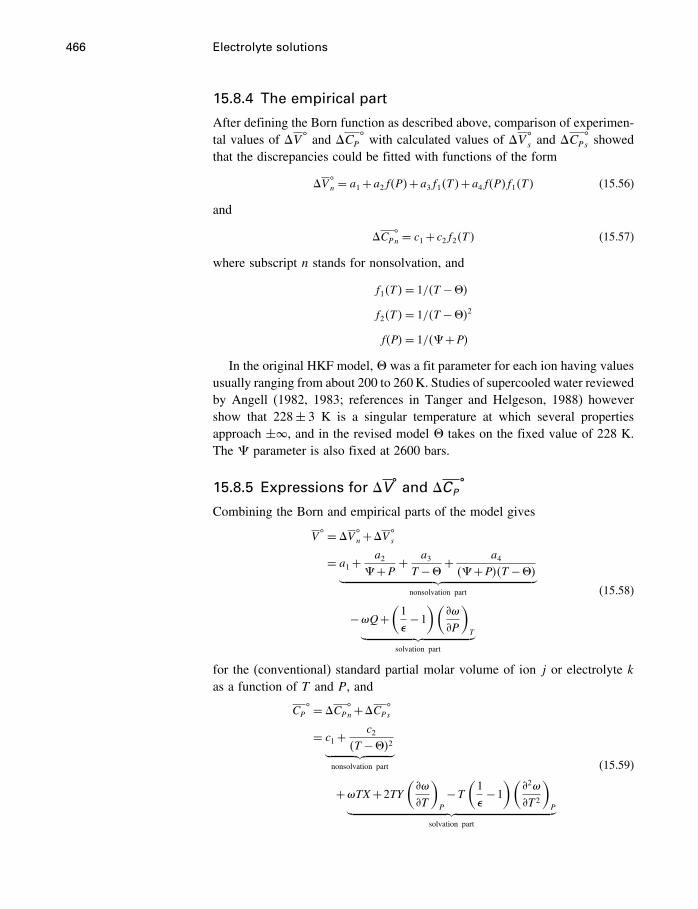
466 Electrolyte solutions
15.8.4 The empirical part
After defining the Born function as described above, comparison of experimen-tal values of �V
�and �CP
�with calculated values of �V
�s and �CP
�s showed
that the discrepancies could be fitted with functions of the form
�V�n = a1+a2f�P�+a3f1�T�+a4f�P�f1�T� (15.56)
and
�CP�n = c1+ c2f2�T� (15.57)
where subscript n stands for nonsolvation, and
f1�T�= 1/�T −"�f2�T�= 1/�T −"�2
f�P�= 1/� +P�In the original HKF model, " was a fit parameter for each ion having values
usually ranging from about 200 to 260K. Studies of supercooled water reviewedby Angell (1982, 1983; references in Tanger and Helgeson, 1988) howevershow that 228± 3 K is a singular temperature at which several propertiesapproach ±�, and in the revised model " takes on the fixed value of 228 K.The parameter is also fixed at 2600 bars.
15.8.5 Expressions for �V�
and �CP�
Combining the Born and empirical parts of the model gives
V� = �V �
n+�V �s
= a1+a2
+P + a3T −" + a4
� +P��T −"�︸ ︷︷ ︸nonsolvation part
−�Q+(1�−1)(
��
�P
)T︸ ︷︷ ︸
solvation part
(15.58)
for the (conventional) standard partial molar volume of ion j or electrolyte kas a function of T and P, and
CP� = �CP
�n+�CP
�s
= c1+c2
�T −"�2︸ ︷︷ ︸nonsolvation part
+�TX+2TY(��
�T
)P
−T(1�−1)(
�2�
�T 2
)P︸ ︷︷ ︸
solvation part
(15.59)
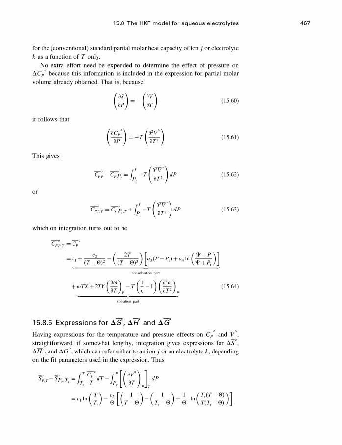
15.8 The HKF model for aqueous electrolytes 467
for the (conventional) standard partial molar heat capacity of ion j or electrolytek as a function of T only.
No extra effort need be expended to determine the effect of pressure on�CP
�because this information is included in the expression for partial molar
volume already obtained. That is, because(�S
�P
)=−
(�V
�T
)(15.60)
it follows that (�CP
�
�P
)=−T
(�2V
�
�T 2
)(15.61)
This gives
CP�P−CP
�Pr
=∫ P
Pr
−T(�2V
�
�T 2
)dP (15.62)
or
CP�P�T = CP
�Pr �T
+∫ P
Pr
−T(�2V
�
�T 2
)dP (15.63)
which on integration turns out to be
CP�P�T = CP
�
= c1+c2
�T −"�2 −(
2T�T −"�3
)[a3�P−Pr�+a4 ln
( +P +Pr
)]︸ ︷︷ ︸
nonsolvation part
+�TX+2TY(��
�T
)P
−T(1�−1)(
�2�
�T 2
)P︸ ︷︷ ︸
solvation part
(15.64)
15.8.6 Expressions for �S�, �H
�and �G
�
Having expressions for the temperature and pressure effects on CP�and V
�,
straightforward, if somewhat lengthy, integration gives expressions for �S�,
�H�, and �G
�, which can refer either to an ion j or an electrolyte k, depending
on the fit parameters used in the expression. Thus
S�P�T −S�Pr �Tr
=∫ T
Tr
CP�
TdT −
∫ P
Pr
[(�V
�
�T
)P
]T
dP
= c1 ln(T
Tr
)− c2"
[(1
T −")−(
1Tr −"
)+ 1"
· ln(Tr�T −"�T�Tr −"�
)]
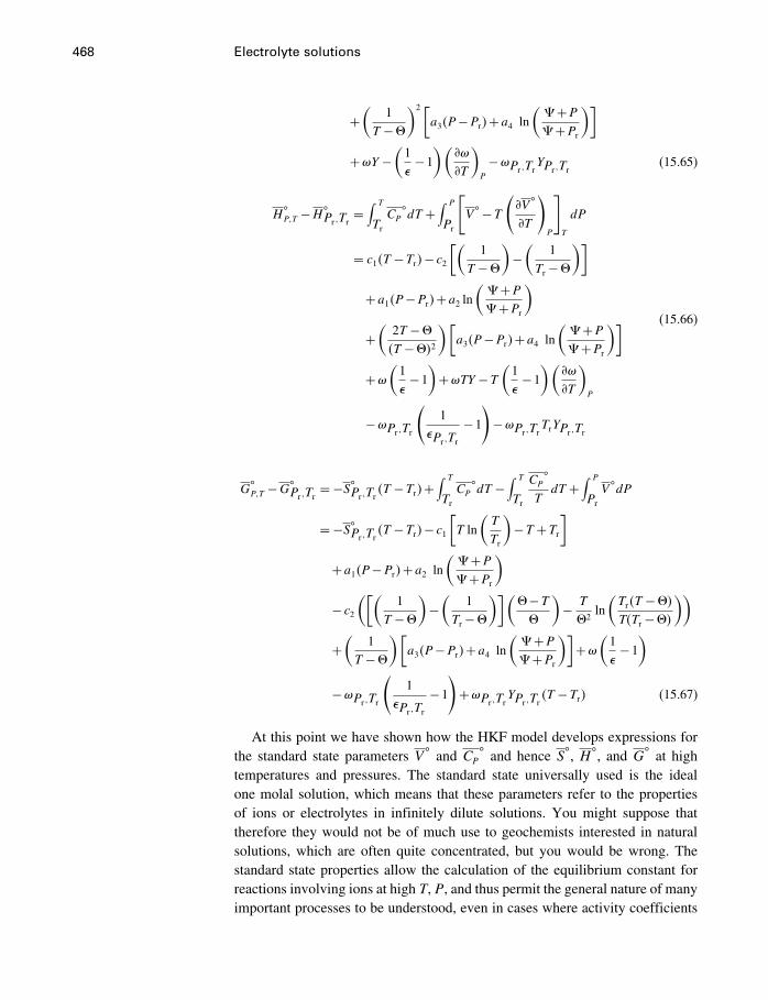
468 Electrolyte solutions
+(
1T −"
)2 [a3�P−Pr�+a4 ln
( +P +Pr
)]+�Y −
(1�−1)(
��
�T
)P
−�Pr �TrYPr �Tr
(15.65)
H�P�T −H�
Pr �Tr=∫ T
TrCP
�dT +
∫ P
Pr
[V
� −T(�V
�
�T
)P
]T
dP
= c1�T −Tr�− c2[(
1T −"
)−(
1Tr −"
)]+a1�P−Pr�+a2 ln
( +P +Pr
)+(
2T −"�T −"�2
)[a3�P−Pr�+a4 ln
( +P +Pr
)]+�
(1�−1)+�TY −T
(1�−1)(
��
�T
)P
−�Pr �Tr
(1
�Pr �Tr−1
)−�Pr �Tr
TrYPr �Tr
(15.66)
G�P�T −G�
Pr �Tr=−S�Pr �Tr
�T −Tr�+∫ T
TrCP
�dT −
∫ T
Tr
CP�
TdT +
∫ P
Pr
V�dP
=−S�Pr �Tr�T −Tr�− c1
[T ln
(T
Tr
)−T +Tr
]+a1�P−Pr�+a2 ln
( +P +Pr
)− c2
([(1
T −")−(
1Tr −"
)]("−T"
)− T
"2ln(Tr�T −"�T�Tr −"�
))+(
1T −"
)[a3�P−Pr�+a4 ln
( +P +Pr
)]+�
(1�−1)
−�Pr �Tr
(1
�Pr �Tr−1
)+�Pr �Tr
YPr �Tr�T −Tr� (15.67)
At this point we have shown how the HKF model develops expressions forthe standard state parameters V
�and CP
�and hence S
�, H
�, and G
�at high
temperatures and pressures. The standard state universally used is the idealone molal solution, which means that these parameters refer to the propertiesof ions or electrolytes in infinitely dilute solutions. You might suppose thattherefore they would not be of much use to geochemists interested in naturalsolutions, which are often quite concentrated, but you would be wrong. Thestandard state properties allow the calculation of the equilibrium constant forreactions involving ions at high T�P, and thus permit the general nature of manyimportant processes to be understood, even in cases where activity coefficients
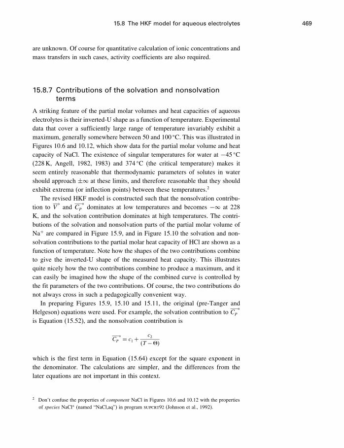
15.8 The HKF model for aqueous electrolytes 469
are unknown. Of course for quantitative calculation of ionic concentrations andmass transfers in such cases, activity coefficients are also required.
15.8.7 Contributions of the solvation and nonsolvationterms
A striking feature of the partial molar volumes and heat capacities of aqueouselectrolytes is their inverted-U shape as a function of temperature. Experimentaldata that cover a sufficiently large range of temperature invariably exhibit amaximum, generally somewhere between 50 and 100 �C. This was illustrated inFigures 10.6 and 10.12, which show data for the partial molar volume and heatcapacity of NaCl. The existence of singular temperatures for water at −45 �C(228K, Angell, 1982, 1983) and 374 �C (the critical temperature) makes itseem entirely reasonable that thermodynamic parameters of solutes in watershould approach ±� at these limits, and therefore reasonable that they shouldexhibit extrema (or inflection points) between these temperatures.2
The revised HKF model is constructed such that the nonsolvation contribu-tion to V
�and CP
�dominates at low temperatures and becomes −� at 228
K, and the solvation contribution dominates at high temperatures. The contri-butions of the solvation and nonsolvation parts of the partial molar volume ofNa+ are compared in Figure 15.9, and in Figure 15.10 the solvation and non-solvation contributions to the partial molar heat capacity of HCl are shown as afunction of temperature. Note how the shapes of the two contributions combineto give the inverted-U shape of the measured heat capacity. This illustratesquite nicely how the two contributions combine to produce a maximum, and itcan easily be imagined how the shape of the combined curve is controlled bythe fit parameters of the two contributions. Of course, the two contributions donot always cross in such a pedagogically convenient way.
In preparing Figures 15.9, 15.10 and 15.11, the original (pre-Tanger andHelgeson) equations were used. For example, the solvation contribution to CP
�
is Equation (15.52), and the nonsolvation contribution is
CP� = c1+
c2�T −"�
which is the first term in Equation (15.64) except for the square exponent inthe denominator. The calculations are simpler, and the differences from thelater equations are not important in this context.
2 Don’t confuse the properties of component NaCl in Figures 10.6 and 10.12 with the propertiesof species NaCl� (named “NaCl,aq”) in program supcrt92 (Johnson et al., 1992).
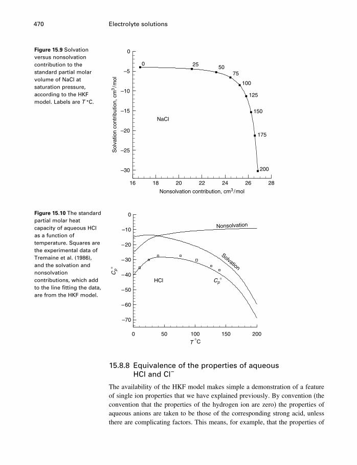
470 Electrolyte solutions
Figure 15.9 Solvationversus nonsolvationcontribution to thestandard partial molarvolume of NaCl atsaturation pressure,according to the HKFmodel. Labels are T �C.
Nonsolvation contribution, cm3/mol
Sol
vatio
n co
ntrib
utio
n, c
m3/m
ol
16 18 20 22 24 26 28
–30
–25
–20
–15
–10
–5
0
0 25 5075
100
125
150
175
200
NaCl
Figure 15.10 The standardpartial molar heatcapacity of aqueous HClas a function oftemperature. Squares arethe experimental data ofTremaine et al. (1986),and the solvation andnonsolvationcontributions, which addto the line fitting the data,are from the HKF model.
Cp°
Cp°
T °C0 50 100 150 200
–10
–20
–30
–40
–50
–60
–70
0
Nonsolvation
Solvation
HCl
15.8.8 Equivalence of the properties of aqueousHCl and Cl−
The availability of the HKF model makes simple a demonstration of a featureof single ion properties that we have explained previously. By convention (theconvention that the properties of the hydrogen ion are zero) the properties ofaqueous anions are taken to be those of the corresponding strong acid, unlessthere are complicating factors. This means, for example, that the properties of
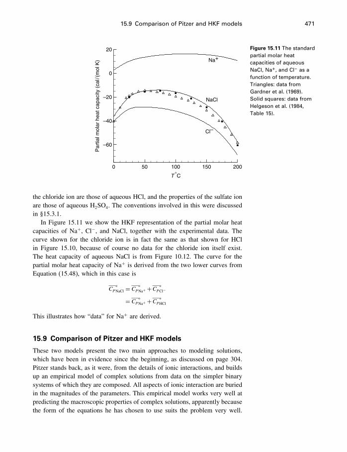
15.9 Comparison of Pitzer and HKF models 471
T °C
Par
tial m
olar
hea
t cap
acity
(ca
l/(m
ol K
)
0 50 100 150 200
0
20
–20
–40
–60
Na+
Cl–
NaCl
Figure 15.11 The standardpartial molar heatcapacities of aqueousNaCl, Na+, and Cl− as afunction of temperature.Triangles: data fromGardner et al. (1969).Solid squares: data fromHelgeson et al. (1984,Table 15).
the chloride ion are those of aqueous HCl, and the properties of the sulfate ionare those of aqueous H2SO4. The conventions involved in this were discussedin §15.3.1.
In Figure 15.11 we show the HKF representation of the partial molar heatcapacities of Na+, Cl−, and NaCl, together with the experimental data. Thecurve shown for the chloride ion is in fact the same as that shown for HClin Figure 15.10, because of course no data for the chloride ion itself exist.The heat capacity of aqueous NaCl is from Figure 10.12. The curve for thepartial molar heat capacity of Na+ is derived from the two lower curves fromEquation (15.48), which in this case is
CP�NaCl = CP
�Na+ +CP
�Cl−
= CP�Na+ +CP
�HCl
This illustrates how “data” for Na+ are derived.
15.9 Comparison of Pitzer and HKF models
These two models present the two main approaches to modeling solutions,which have been in evidence since the beginning, as discussed on page 304.Pitzer stands back, as it were, from the details of ionic interactions, and buildsup an empirical model of complex solutions from data on the simpler binarysystems of which they are composed. All aspects of ionic interaction are buriedin the magnitudes of the parameters. This empirical model works very well atpredicting the macroscopic properties of complex solutions, apparently becausethe form of the equations he has chosen to use suits the problem very well.
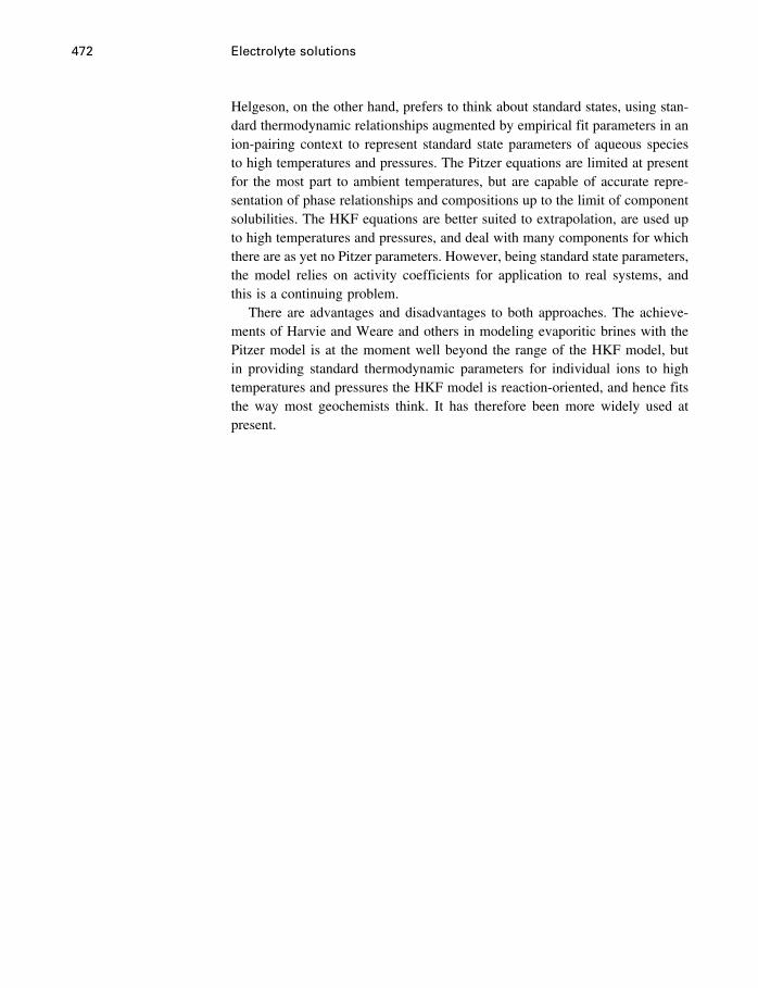
472 Electrolyte solutions
Helgeson, on the other hand, prefers to think about standard states, using stan-dard thermodynamic relationships augmented by empirical fit parameters in anion-pairing context to represent standard state parameters of aqueous speciesto high temperatures and pressures. The Pitzer equations are limited at presentfor the most part to ambient temperatures, but are capable of accurate repre-sentation of phase relationships and compositions up to the limit of componentsolubilities. The HKF equations are better suited to extrapolation, are used upto high temperatures and pressures, and deal with many components for whichthere are as yet no Pitzer parameters. However, being standard state parameters,the model relies on activity coefficients for application to real systems, andthis is a continuing problem.
There are advantages and disadvantages to both approaches. The achieve-ments of Harvie and Weare and others in modeling evaporitic brines with thePitzer model is at the moment well beyond the range of the HKF model, butin providing standard thermodynamic parameters for individual ions to hightemperatures and pressures the HKF model is reaction-oriented, and hence fitsthe way most geochemists think. It has therefore been more widely used atpresent.
16Rock–water systems
16.1 Real problems
We have now completed our survey of the thermodynamic principles requiredto model natural systems. It only remains to gain practice in formulatingproblems involving natural systems in thermodynamic terms. Quite often, thatis the hardest part. Once the problem is set up in terms of relevant reactionsand components, the equations can be solved by anyone who has absorbed theprevious chapters. However, choosing the appropriate components and settingup the relevant balanced reactions only comes from experience. In this chapterwe explore a few situations that have been investigated by thermodynamicmethods.
16.2 Is the sea saturated with calcium carbonate?
If you have ever been to Florida or the Bahamas, you may be aware that thereare vast areas adjacent to the coasts where the sea bottom at shallow levels isa white mud, which turns out to be made of almost pure aragonite. Carbonatemuds extend well out to the deep sea as well; in fact, a fairly large proportionof the sea bottom is composed of calcium carbonate. There are also countlesscalcitic atolls and reefs throughout the tropical zones of the world. Giventhis amount of contact between the sea and calcium carbonate, both calciteand aragonite, plus the fact that there are vigorous oceanic currents stirringthings up constantly, plus the fact that things have not changed drastically formillions of years, you would think that there would be little doubt that thesystem consisting of the oceans plus their bottom sediments must have reachedequilibrium by now. If these were the only factors involved, perhaps they wouldhave, but the situation is quite a bit more complicated. Why would anyonewant to know? Reactions involving carbonate in the oceans are fundamentalto an understanding of the global CO2 cycle, which in turn is linked to globalwarming and other things we would like to understand.
How do you tell if a solution is saturated?To explore this problem further, we must first find out how to determinewhether a solution is saturated, undersaturated, or supersaturated with a given
473
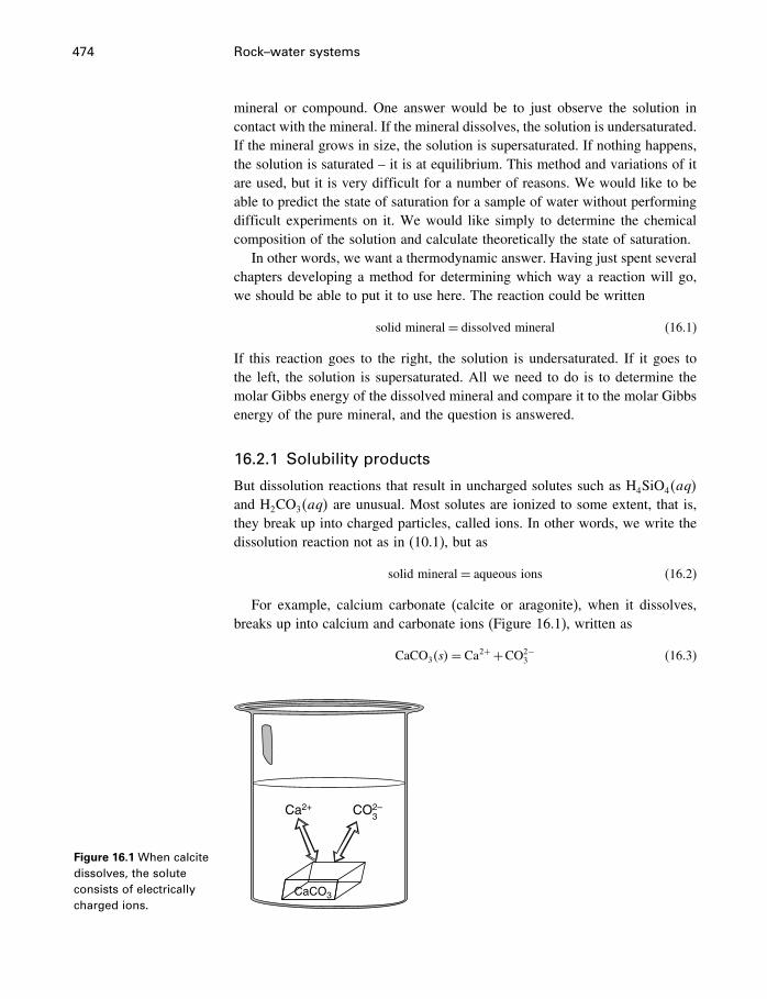
474 Rock–water systems
mineral or compound. One answer would be to just observe the solution incontact with the mineral. If the mineral dissolves, the solution is undersaturated.If the mineral grows in size, the solution is supersaturated. If nothing happens,the solution is saturated – it is at equilibrium. This method and variations of itare used, but it is very difficult for a number of reasons. We would like to beable to predict the state of saturation for a sample of water without performingdifficult experiments on it. We would like simply to determine the chemicalcomposition of the solution and calculate theoretically the state of saturation.
In other words, we want a thermodynamic answer. Having just spent severalchapters developing a method for determining which way a reaction will go,we should be able to put it to use here. The reaction could be written
solid mineral= dissolved mineral (16.1)
If this reaction goes to the right, the solution is undersaturated. If it goes tothe left, the solution is supersaturated. All we need to do is to determine themolar Gibbs energy of the dissolved mineral and compare it to the molar Gibbsenergy of the pure mineral, and the question is answered.
16.2.1 Solubility products
But dissolution reactions that result in uncharged solutes such as H4SiO4�aq�
and H2CO3�aq� are unusual. Most solutes are ionized to some extent, that is,they break up into charged particles, called ions. In other words, we write thedissolution reaction not as in (10.1), but as
solid mineral= aqueous ions (16.2)
For example, calcium carbonate (calcite or aragonite), when it dissolves,breaks up into calcium and carbonate ions (Figure 16.1), written as
CaCO3�s�= Ca2++CO2−3 (16.3)
Figure 16.1 When calcitedissolves, the soluteconsists of electricallycharged ions.
Ca2+ CO2–3
CaCO3
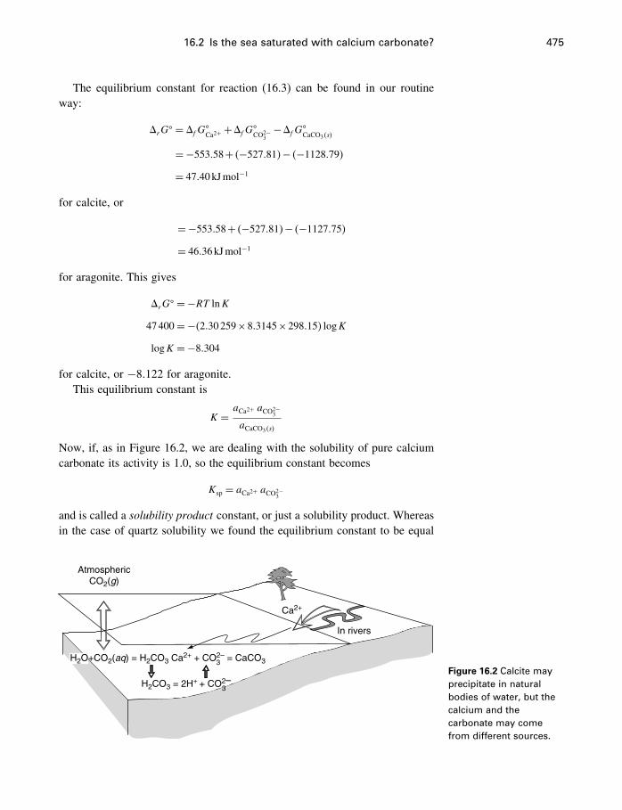
16.2 Is the sea saturated with calcium carbonate? 475
The equilibrium constant for reaction (16.3) can be found in our routineway:
�rG� = �fG
�Ca2+ +�fG
�CO2−
3−�fG
�CaCO3�s�
=−553�58+ �−527�81�− �−1128�79�
= 47�40kJmol−1
for calcite, or
=−553�58+ �−527�81�− �−1127�75�
= 46�36kJmol−1
for aragonite. This gives
�rG� = −RT lnK
47400=−�2�30259×8�3145×298�15� logK
logK =−8�304
for calcite, or −8�122 for aragonite.This equilibrium constant is
K = aCa2+ aCO2−3
aCaCO3�s�
Now, if, as in Figure 16.2, we are dealing with the solubility of pure calciumcarbonate its activity is 1.0, so the equilibrium constant becomes
Ksp = aCa2+ aCO2−3
and is called a solubility product constant, or just a solubility product. Whereasin the case of quartz solubility we found the equilibrium constant to be equal
AtmosphericCO2(g)
In rivers
H2CO3 = 2H+ + CO2–3
Ca2+
H2O+CO2(aq) = H2CO3 Ca2+ + CO2– = CaCO33Figure 16.2 Calcite mayprecipitate in naturalbodies of water, but thecalcium and thecarbonate may comefrom different sources.
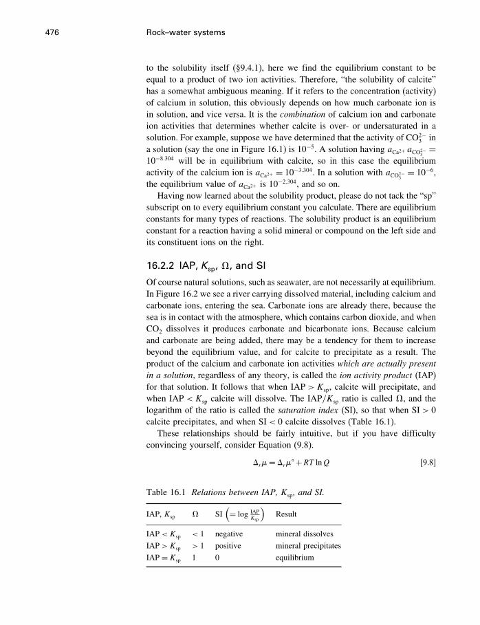
476 Rock–water systems
to the solubility itself (§9.4.1), here we find the equilibrium constant to beequal to a product of two ion activities. Therefore, “the solubility of calcite”has a somewhat ambiguous meaning. If it refers to the concentration (activity)of calcium in solution, this obviously depends on how much carbonate ion isin solution, and vice versa. It is the combination of calcium ion and carbonateion activities that determines whether calcite is over- or undersaturated in asolution. For example, suppose we have determined that the activity of CO2−
3 ina solution (say the one in Figure 16.1) is 10−5. A solution having aCa2+ aCO2−
3=
10−8�304 will be in equilibrium with calcite, so in this case the equilibriumactivity of the calcium ion is aCa2+ = 10−3�304. In a solution with aCO2−
3= 10−6,
the equilibrium value of aCa2+ is 10−2�304, and so on.Having now learned about the solubility product, please do not tack the “sp”
subscript on to every equilibrium constant you calculate. There are equilibriumconstants for many types of reactions. The solubility product is an equilibriumconstant for a reaction having a solid mineral or compound on the left side andits constituent ions on the right.
16.2.2 IAP, Ksp, , and SI
Of course natural solutions, such as seawater, are not necessarily at equilibrium.In Figure 16.2 we see a river carrying dissolved material, including calcium andcarbonate ions, entering the sea. Carbonate ions are already there, because thesea is in contact with the atmosphere, which contains carbon dioxide, and whenCO2 dissolves it produces carbonate and bicarbonate ions. Because calciumand carbonate are being added, there may be a tendency for them to increasebeyond the equilibrium value, and for calcite to precipitate as a result. Theproduct of the calcium and carbonate ion activities which are actually presentin a solution, regardless of any theory, is called the ion activity product (IAP)for that solution. It follows that when IAP > Ksp, calcite will precipitate, andwhen IAP < Ksp calcite will dissolve. The IAP/Ksp ratio is called #, and thelogarithm of the ratio is called the saturation index (SI), so that when SI > 0calcite precipitates, and when SI < 0 calcite dissolves (Table 16.1).
These relationships should be fairly intuitive, but if you have difficultyconvincing yourself, consider Equation (9.8).
�r�= �r�� +RT lnQ [9.8]
Table 16.1 Relations between IAP, Ksp, and SI.
IAP, Ksp # SI(= log IAP
Ksp
)Result
IAP <Ksp < 1 negative mineral dissolves
IAP >Ksp > 1 positive mineral precipitates
IAP = Ksp 1 0 equilibrium
16.3 Determining the IAP – speciation 477
In the case we are considering – calcite and its ions, reaction (16.3) – whenQ= Ksp, �r�= 0. Therefore, if Q= IAP >Ksp, �r� > 0, and reaction (16.3)will go to the left (calcite precipitates). And if Q = IAP < Ksp, �r� < 0,reaction (16.3) will go to the right (calcite dissolves).
16.3 Determining the IAP – speciation
Now to answer our question as to whether the sea is saturated with calcite,we need only determine its IAP and compare it with Ksp for calcite. Easiersaid than done. Apart from some specialized electrochemical techniques, it isgenerally not possible to analyze a solution for the concentration of specificions such as Ca2+ or CO2−
3 . Analyses are made for the total calcium, or thetotal carbonate in the solution. There are many kinds of ions and unchargedmolecular species such as ion-pairs in a solution, and so the total calciumconcentration would consist of the sum of the concentrations of all the ionicand molecular species containing Ca, and similarly for carbonate. Thus
mCa�total =mCa2+ +mCaHCO+3+mCaSO�
4+· · ·
mCO3�total=mCO2−
3+mHCO−
3+mH2CO3
+· · ·Here, CaSO�
4 represents an electrically neutral species resulting from the joiningof a Ca2+ ion and a SO2−
4 ion in solution. There are several more species in eachof these summations in real seawater which we won’t mention. But howevermany there are, the concentrations and activities of all of them can be calculatedif for every species there is a known equilibrium constant relating it to otherspecies and/or minerals, and if there is a suitable equation for calculating theactivity coefficients (H) of each of the species.
What it amounts to is the well-known fact that if in a set of equations youhave the same number of equations as you have variables, it is possible to solvefor every variable. Given the total concentrations of the various constituents ofseawater (not only calcium and carbonate, but however many you are interestedin), plus an equilibrium constant for each, plus the knowledge that the totalpositive charges must equal the total negative charges, it is always possible toachieve this goal. When more than a few ions are involved, the procedure canbe carried out only on a computer, and many programs are now available fordoing this.
It is also worth pointing out that the process of speciation is mathematicallyequivalent to finding the system configuration which minimizes the Gibbsenergy. This can be shown formally, but if you think of reactions which havenot equilibrated as being somewhere above the minimum on a U-shaped Gibbsenergy versus progress variable curve (see Figure 18.8 for an example), andbeing at the minimum when at equilibrium, it should be fairly intuitive. Whenall possible reactions achieve their minimum Gibbs energy, then so does thesystem.
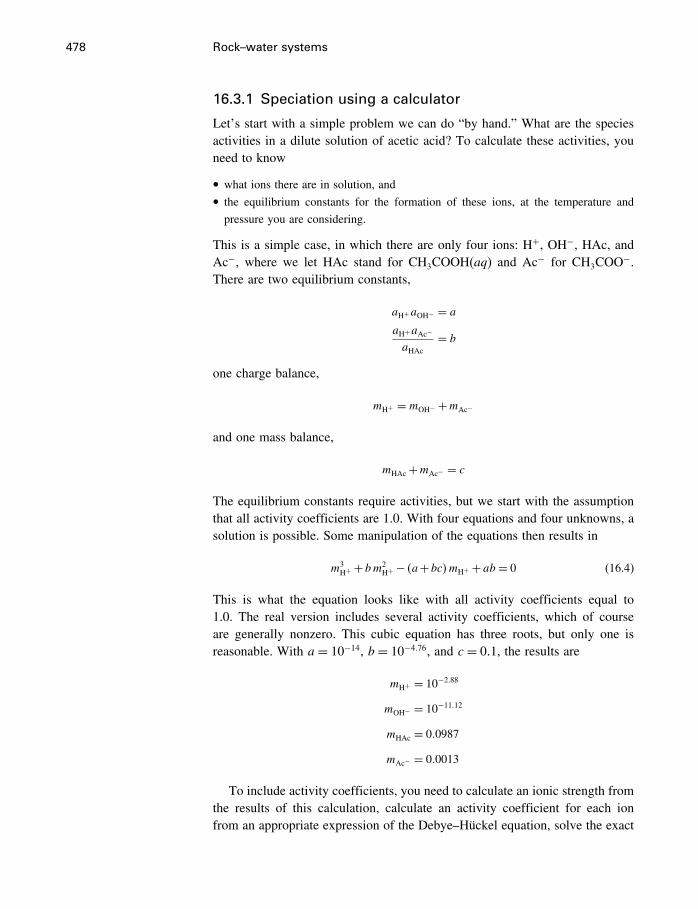
478 Rock–water systems
16.3.1 Speciation using a calculator
Let’s start with a simple problem we can do “by hand.” What are the speciesactivities in a dilute solution of acetic acid? To calculate these activities, youneed to know
• what ions there are in solution, and• the equilibrium constants for the formation of these ions, at the temperature and
pressure you are considering.
This is a simple case, in which there are only four ions: H+, OH−, HAc, andAc−, where we let HAc stand for CH3COOH(aq) and Ac− for CH3COO
−.There are two equilibrium constants,
aH+aOH− = aaH+aAc−
aHAc= b
one charge balance,
mH+ =mOH− +mAc−
and one mass balance,
mHAc+mAc− = c
The equilibrium constants require activities, but we start with the assumptionthat all activity coefficients are 1.0. With four equations and four unknowns, asolution is possible. Some manipulation of the equations then results in
m3H+ +bm2
H+ − �a+bc�mH+ +ab = 0 (16.4)
This is what the equation looks like with all activity coefficients equal to1.0. The real version includes several activity coefficients, which of courseare generally nonzero. This cubic equation has three roots, but only one isreasonable. With a= 10−14, b = 10−4�76, and c = 0�1, the results are
mH+ = 10−2�88
mOH− = 10−11�12
mHAc = 0�0987
mAc− = 0�0013
To include activity coefficients, you need to calculate an ionic strength fromthe results of this calculation, calculate an activity coefficient for each ionfrom an appropriate expression of the Debye–Hückel equation, solve the exact
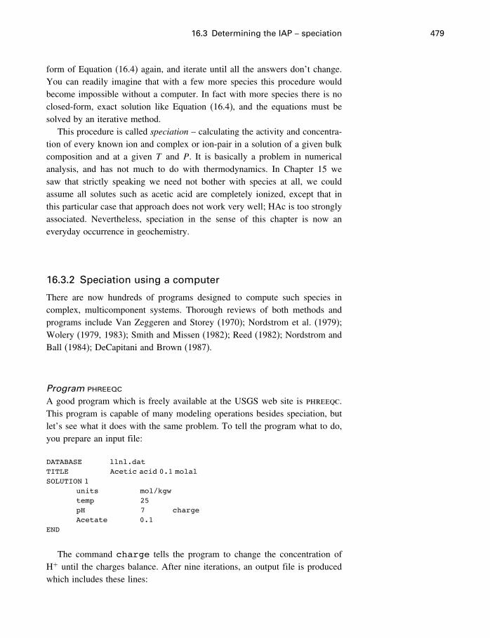
16.3 Determining the IAP – speciation 479
form of Equation (16.4) again, and iterate until all the answers don’t change.You can readily imagine that with a few more species this procedure wouldbecome impossible without a computer. In fact with more species there is noclosed-form, exact solution like Equation (16.4), and the equations must besolved by an iterative method.
This procedure is called speciation – calculating the activity and concentra-tion of every known ion and complex or ion-pair in a solution of a given bulkcomposition and at a given T and P. It is basically a problem in numericalanalysis, and has not much to do with thermodynamics. In Chapter 15 wesaw that strictly speaking we need not bother with species at all, we couldassume all solutes such as acetic acid are completely ionized, except that inthis particular case that approach does not work very well; HAc is too stronglyassociated. Nevertheless, speciation in the sense of this chapter is now aneveryday occurrence in geochemistry.
16.3.2 Speciation using a computer
There are now hundreds of programs designed to compute such species incomplex, multicomponent systems. Thorough reviews of both methods andprograms include Van Zeggeren and Storey (1970); Nordstrom et al. (1979);Wolery (1979, 1983); Smith and Missen (1982); Reed (1982); Nordstrom andBall (1984); DeCapitani and Brown (1987).
Program phreeqcA good program which is freely available at the USGS web site is phreeqc.This program is capable of many modeling operations besides speciation, butlet’s see what it does with the same problem. To tell the program what to do,you prepare an input file:
DATABASE llnl.datTITLE Acetic acid 0.1 molalSOLUTION 1
units mol/kgwtemp 25pH 7 chargeAcetate 0.1
END
The command charge tells the program to change the concentration ofH+ until the charges balance. After nine iterations, an output file is producedwhich includes these lines:
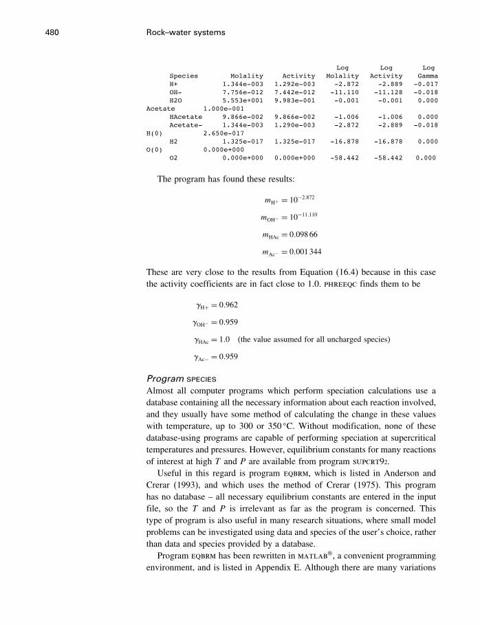
480 Rock–water systems
Log Log LogSpecies Molality Activity Molality Activity GammaH+ 1.344e-003 1.292e-003 -2.872 -2.889 -0.017OH- 7.756e-012 7.442e-012 -11.110 -11.128 -0.018H2O 5.553e+001 9.983e-001 -0.001 -0.001 0.000
Acetate 1.000e-001HAcetate 9.866e-002 9.866e-002 -1.006 -1.006 0.000Acetate- 1.344e-003 1.290e-003 -2.872 -2.889 -0.018
H(0) 2.650e-017H2 1.325e-017 1.325e-017 -16.878 -16.878 0.000
O(0) 0.000e+000O2 0.000e+000 0.000e+000 -58.442 -58.442 0.000
The program has found these results:
mH+ = 10−2�872
mOH− = 10−11�110
mHAc = 0�09866
mAc− = 0�001344
These are very close to the results from Equation (16.4) because in this casethe activity coefficients are in fact close to 1.0. phreeqc finds them to be
H+ = 0�962
OH− = 0�959
HAc = 1�0 (the value assumed for all uncharged species)
Ac− = 0�959
Program speciesAlmost all computer programs which perform speciation calculations use adatabase containing all the necessary information about each reaction involved,and they usually have some method of calculating the change in these valueswith temperature, up to 300 or 350 �C. Without modification, none of thesedatabase-using programs are capable of performing speciation at supercriticaltemperatures and pressures. However, equilibrium constants for many reactionsof interest at high T and P are available from program supcrt92.
Useful in this regard is program eqbrm, which is listed in Anderson andCrerar (1993), and which uses the method of Crerar (1975). This programhas no database – all necessary equilibrium constants are entered in the inputfile, so the T and P is irrelevant as far as the program is concerned. Thistype of program is also useful in many research situations, where small modelproblems can be investigated using data and species of the user’s choice, ratherthan data and species provided by a database.
Program eqbrm has been rewritten in matlab®, a convenient programmingenvironment, and is listed in Appendix E. Although there are many variations
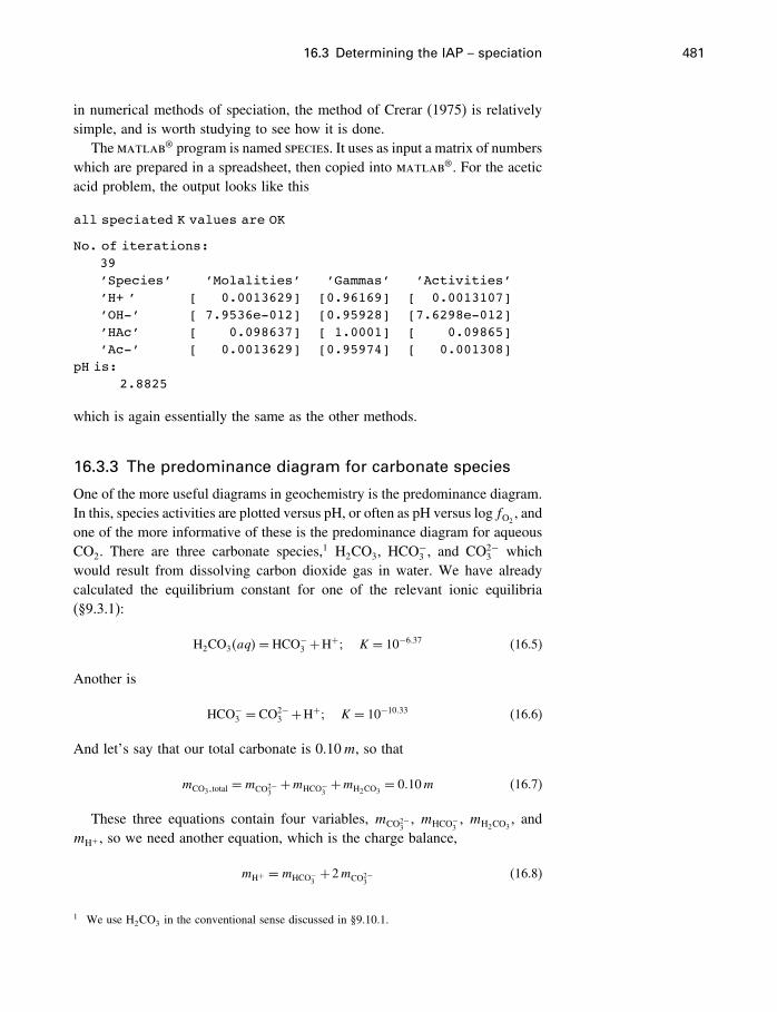
16.3 Determining the IAP – speciation 481
in numerical methods of speciation, the method of Crerar (1975) is relativelysimple, and is worth studying to see how it is done.
The matlab® program is named species. It uses as input a matrix of numberswhich are prepared in a spreadsheet, then copied into matlab®. For the aceticacid problem, the output looks like this
all speciated K values are OK
No. of iterations:39’Species’ ’Molalities’ ’Gammas’ ’Activities’’H+ ’ [ 0.0013629] [0.96169] [ 0.0013107]’OH-’ [ 7.9536e-012] [0.95928] [7.6298e-012]’HAc’ [ 0.098637] [ 1.0001] [ 0.09865]’Ac-’ [ 0.0013629] [0.95974] [ 0.001308]
pH is:2.8825
which is again essentially the same as the other methods.
16.3.3 The predominance diagram for carbonate species
One of the more useful diagrams in geochemistry is the predominance diagram.In this, species activities are plotted versus pH, or often as pH versus logfO2
, andone of the more informative of these is the predominance diagram for aqueousCO2. There are three carbonate species,1 H2CO3, HCO
−3 , and CO2−
3 whichwould result from dissolving carbon dioxide gas in water. We have alreadycalculated the equilibrium constant for one of the relevant ionic equilibria(§9.3.1):
H2CO3�aq�= HCO−3 +H+� K = 10−6�37 (16.5)
Another is
HCO−3 = CO2−
3 +H+� K = 10−10�33 (16.6)
And let’s say that our total carbonate is 0.10m, so that
mCO3�total=mCO2−
3+mHCO−
3+mH2CO3
= 0�10m (16.7)
These three equations contain four variables, mCO2−3, mHCO−
3, mH2CO3
, andmH+ , so we need another equation, which is the charge balance,
mH+ =mHCO−3+2mCO2−
3(16.8)
1 We use H2CO3 in the conventional sense discussed in §9.10.1.
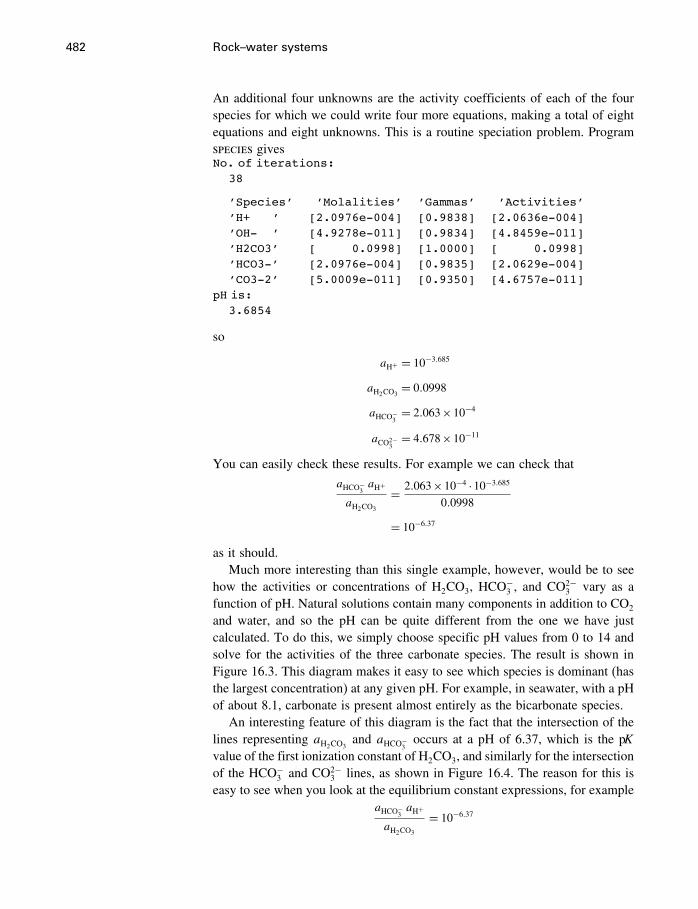
482 Rock–water systems
An additional four unknowns are the activity coefficients of each of the fourspecies for which we could write four more equations, making a total of eightequations and eight unknowns. This is a routine speciation problem. Programspecies givesNo. of iterations:
38
’Species’ ’Molalities’ ’Gammas’ ’Activities’’H+ ’ [2.0976e-004] [0.9838] [2.0636e-004]’OH- ’ [4.9278e-011] [0.9834] [4.8459e-011]’H2CO3’ [ 0.0998] [1.0000] [ 0.0998]’HCO3-’ [2.0976e-004] [0.9835] [2.0629e-004]’CO3-2’ [5.0009e-011] [0.9350] [4.6757e-011]
pH is:3.6854
so
aH+ = 10−3�685
aH2CO3= 0�0998
aHCO−3= 2�063×10−4
aCO2−3
= 4�678×10−11
You can easily check these results. For example we can check that
aHCO−3aH+
aH2CO3
= 2�063×10−4 ·10−3�685
0�0998
= 10−6�37
as it should.Much more interesting than this single example, however, would be to see
how the activities or concentrations of H2CO3, HCO−3 , and CO2−
3 vary as afunction of pH. Natural solutions contain many components in addition to CO2
and water, and so the pH can be quite different from the one we have justcalculated. To do this, we simply choose specific pH values from 0 to 14 andsolve for the activities of the three carbonate species. The result is shown inFigure 16.3. This diagram makes it easy to see which species is dominant (hasthe largest concentration) at any given pH. For example, in seawater, with a pHof about 8.1, carbonate is present almost entirely as the bicarbonate species.
An interesting feature of this diagram is the fact that the intersection of thelines representing aH2CO3
and aHCO−3occurs at a pH of 6.37, which is the pK
value of the first ionization constant of H2CO3, and similarly for the intersectionof the HCO−
3 and CO2−3 lines, as shown in Figure 16.4. The reason for this is
easy to see when you look at the equilibrium constant expressions, for exampleaHCO−
3aH+
aH2CO3
= 10−6�37
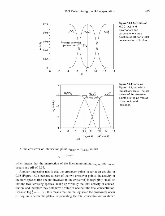
16.3 Determining the IAP – speciation 483
0.10
0.08
0.06
0.04
0.02
0
Act
ivity
0 2 4 6 8 10 12 14
Average seawater pH = 8.1–8.2
H2CO3 HCO3–
pH
–CO23
Figure 16.3 Activities ofH2CO3�aq�, andbicarbonate andcarbonate ions as afunction of pH, for a totalconcentration of 0.10m.
pHpK1=6.37 pK2=10.33
0 2 4 6 8 10 12 14
log
activ
ity
–4
–3
–2
–1
0
H2CO3 HCO3–
0.3 log units
2–CO3
Figure 16.4 Same asFigure 16.3, but with alog activity scale. The pHvalues of the crossoverpoints are the pK valuesof carbonic acidionization.
At the crossover or intersection point, aHCO−3= aH2CO3
, so that
aH+ = 10−6�37
which means that the intersection of the lines representing aH2CO3and aHCO−
3
occurs at a pH of 6.37.Another interesting fact is that the crossover points occur at an activity of
0.05 (Figure 16.3), because at each of the two crossover points, the activity ofthe third species (the one not involved in the crossover) is negligibly small, sothat the two “crossing species” make up virtually the total activity or concen-tration, and therefore they both have a value of one-half the total concentration.Because log 1
2 = −0�30, this means that on the log scale the crossovers occur0.3 log units below the plateau representing the total concentration, as shown
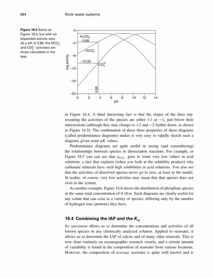
484 Rock–water systems
Figure 16.5 Same asFigure 16.4, but with anexpanded activity axis.At a pH of 3.69, the HCO−
3
and CO2−3 activities are
those calculated in thetext.
pH0 2 4 6 8 10 12 14
log
activ
ity
–20
–16
–12
–8
–4
0
H2CO3
HCO3–
2–CO3
–3.69
–10.33
3.69
in Figure 16.4. A third interesting fact is that the slopes of the lines rep-resenting the activities of the species are either +1 or −1, just below theirintersections (although they may change to +2 and −2 farther down, as shownin Figure 16.5). The combination of these three properties of these diagrams(called predominance diagrams) makes it very easy to rapidly sketch such adiagram, given some pK values.
Predominance diagrams are quite useful in seeing (and remembering)the relationships between species in dissociation reactions. For example, inFigure 16.5 you can see that aCO2−
3goes to some very low values in acid
solutions, a fact that explains (when you look at the solubility product) whycarbonate minerals have such high solubilities in acid solutions. You also seethat the activities of dissolved species never go to zero, at least in the model.In reality, of course, very low activities may mean that that species does notexist in the system.
As another example, Figure 16.6 shows the distribution of phosphate speciesat the same total concentration of 0�10m. Such diagrams are clearly useful forany solute that can exist in a variety of species, differing only by the numberof hydrogen ions (protons) they have.
16.4 Combining the IAP and the Ksp
So speciation allows us to determine the concentrations and activities of allknown species in any chemically analyzed solution. Applied to seawater, itallows us to determine the IAP of calcite and of many other minerals. This isnow done routinely on oceanographic research vessels, and a certain amountof variability is found in the composition of seawater from various locations.However, the composition of average seawater is quite well known and is
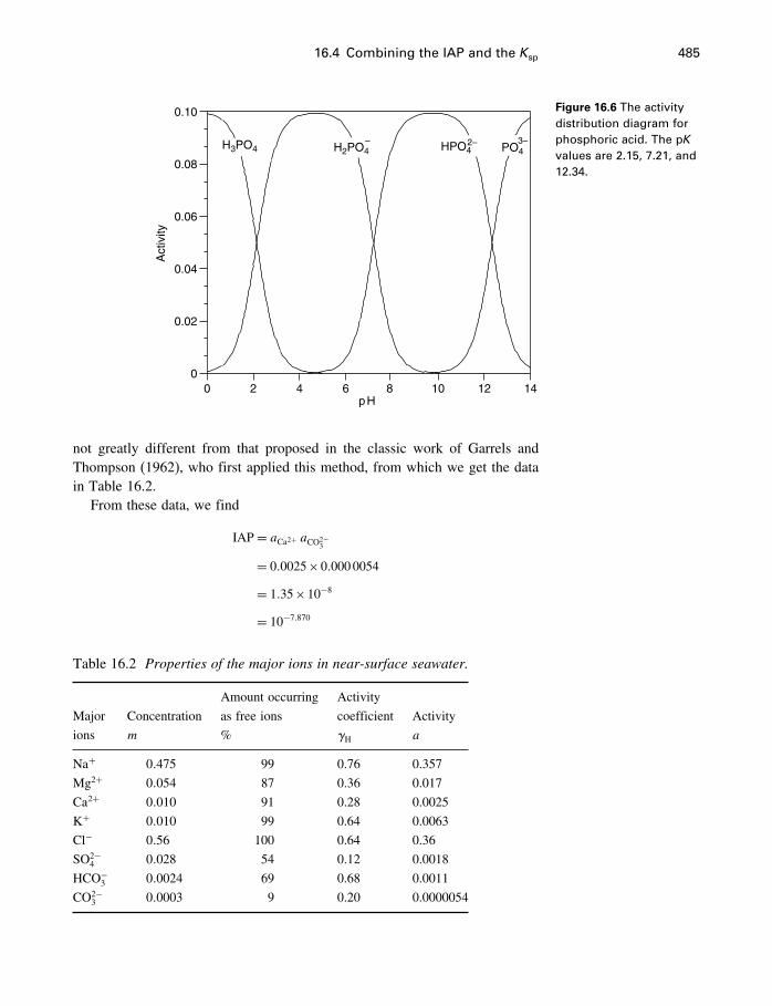
16.4 Combining the IAP and the Ksp 485
Figure 16.6 The activitydistribution diagram forphosphoric acid. The pKvalues are 2.15, 7.21, and12.34.
00
0.02
0.04
0.06
0.08
0.10
2 4 6 8 10 12 14p H
H3PO4 PO43–
H2PO4– HPO4
2–
Act
ivity
not greatly different from that proposed in the classic work of Garrels andThompson (1962), who first applied this method, from which we get the datain Table 16.2.
From these data, we find
IAP= aCa2+ aCO2−3
= 0�0025×0�0000054
= 1�35×10−8
= 10−7�870
Table 16.2 Properties of the major ions in near-surface seawater.
Amount occurring Activity
Major Concentration as free ions coefficient Activity
ions m % H a
Na+ 0�475 99 0.76 0.357
Mg2+ 0�054 87 0.36 0.017
Ca2+ 0�010 91 0.28 0.0025
K+ 0�010 99 0.64 0.0063
Cl− 0�56 100 0.64 0.36
SO2−4 0�028 54 0.12 0.0018
HCO−3 0�0024 69 0.68 0.0011
CO2−3 0�0003 9 0.20 0.0000054
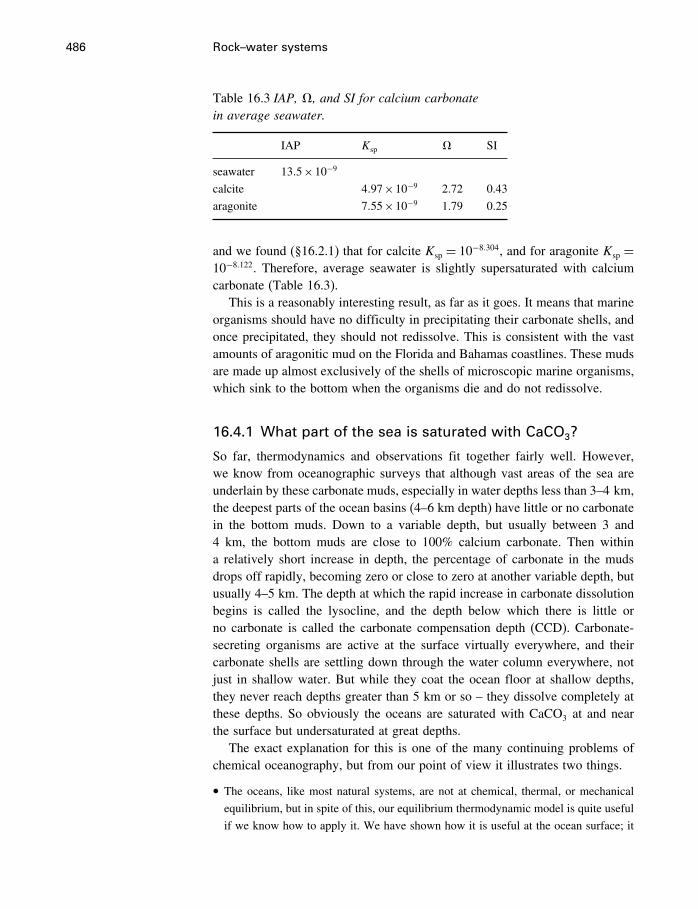
486 Rock–water systems
Table 16.3 IAP, #, and SI for calcium carbonatein average seawater.
IAP Ksp # SI
seawater 13�5×10⁻⁹
calcite 4�97×10−9 2.72 0.43
aragonite 7�55×10−9 1.79 0.25
and we found (§16.2.1) that for calcite Ksp = 10−8�304, and for aragonite Ksp =10−8�122. Therefore, average seawater is slightly supersaturated with calciumcarbonate (Table 16.3).
This is a reasonably interesting result, as far as it goes. It means that marineorganisms should have no difficulty in precipitating their carbonate shells, andonce precipitated, they should not redissolve. This is consistent with the vastamounts of aragonitic mud on the Florida and Bahamas coastlines. These mudsare made up almost exclusively of the shells of microscopic marine organisms,which sink to the bottom when the organisms die and do not redissolve.
16.4.1 What part of the sea is saturated with CaCO3?
So far, thermodynamics and observations fit together fairly well. However,we know from oceanographic surveys that although vast areas of the sea areunderlain by these carbonate muds, especially in water depths less than 3–4 km,the deepest parts of the ocean basins (4–6 km depth) have little or no carbonatein the bottom muds. Down to a variable depth, but usually between 3 and4 km, the bottom muds are close to 100% calcium carbonate. Then withina relatively short increase in depth, the percentage of carbonate in the mudsdrops off rapidly, becoming zero or close to zero at another variable depth, butusually 4–5 km. The depth at which the rapid increase in carbonate dissolutionbegins is called the lysocline, and the depth below which there is little orno carbonate is called the carbonate compensation depth (CCD). Carbonate-secreting organisms are active at the surface virtually everywhere, and theircarbonate shells are settling down through the water column everywhere, notjust in shallow water. But while they coat the ocean floor at shallow depths,they never reach depths greater than 5 km or so – they dissolve completely atthese depths. So obviously the oceans are saturated with CaCO3 at and nearthe surface but undersaturated at great depths.
The exact explanation for this is one of the many continuing problems ofchemical oceanography, but from our point of view it illustrates two things.
• The oceans, like most natural systems, are not at chemical, thermal, or mechanical
equilibrium, but in spite of this, our equilibrium thermodynamic model is quite useful
if we know how to apply it. We have shown how it is useful at the ocean surface; it
16.5 Mineral stability diagrams 487
is also useful at great depth. But obviously it would not be useful to apply it to the
oceans as a whole system – they are too far from equilibrium.• The explanation for the CCD and its variations is complex, involving the kinetics
of carbonate dissolution, variations in ocean chemistry, temperature, and pressure,
worldwide circulation patterns, and other factors. Equilibrium chemical thermody-
namics does not suffice for an understanding of this natural system, but it is invariably
the starting point for all other types of investigation. You must have an understanding
of the equilibrium state before you can understand the departures from this state.
16.5 Mineral stability diagrams
The problem of calcite saturation in the sea is only one of a large numberof problems in oceanography, geology, soil chemistry, and many other areasof science that involve solid�fluid reactions, and a variety of diagrams havebeen used to illustrate the thermodynamic relationships involved. Humans findtwo-dimensional diagrams much easier to understand than multidimensionalsystems of equations.
16.5.1 The reaction of feldspar with water
One of the most common minerals on Earth is feldspar, and its reaction withwater to form other minerals such as clays is of great interest in several fields. Insoils, feldspars (solid solutions of NaAlSi3O8, KAlSi3O8, and CaAl2Si2O8) reactto form clay minerals, helping to control soil acidity. In petroleum reservoirs,the same reaction forming clay minerals can have serious effects on the rockpermeability and oil recovery. K-feldspars often have appreciable amountsof Pb substituting for K in their structures, and reaction of K-feldspar withformation fluids is thought to release this Pb to the fluid, which may then goon to form a lead ore-body elsewhere on its travels through the Earth’s crust.During metamorphism, when rocks containing feldspars are subjected to hightemperatures and pressures deep in the crust, feldspars participate in a varietyof reactions with fluids and with other minerals, all of which are of interest togeologists studying the history of the Earth.
The question for us is, how do we apply thermodynamics to these reactions?The first thing we must do is write a reaction that seems interesting. This isone of the most difficult steps, but one that is rarely discussed because thereare no rules to guide us. There is a very large number of reactions that could bewritten involving K-feldspar, depending on what other things are in the system,but only a few of these are useful. Only experience and scientific insight candistinguish between what might turn out to be useful and what will not. Thereactions that appear in texts have, of course, proven to be useful.
If you were to write a reaction between K-feldspar and kaolinite with noprevious experience or prejudices, but just putting them on opposite sides of
488 Rock–water systems
an equal sign and adding other compounds to balance, you would likely windup with something like this:
KAlSi3O8�s�+ 32H2O�l�= 1
2Al2Si2O5�OH�4�s�+2SiO2+KOH (16.9)
We have not specified whether SiO2 is quartz or SiO2�aq� – you have yourchoice. If you choose quartz, and quartz is present in the system, its activity willbe 1.0; if you choose SiO2�aq�, its activity will be (a dimensionless numberequal to) the molality of silica in solution. Pure KOH is a solid, but it ionizescompletely in solution, and you again have a choice of the �s� or the �aq� formsof data. If we choose to use quartz, KOH�aq�, and the maximum microclineform of KAlSi3O8 (or K-feldspar), the equilibrium constant turns out to be10−7�88, and, because all the products and reactants except KOH have a= 1, atleast if the water is reasonably pure, this turns out to be the molality of KOHin our system. What system? We have not been very specific about what oursystem consists of, other than that it contains K-feldspar, kaolinite, and water,at 25 �C, 1 bar. We might be thinking about a soil with groundwater.
But, you say, groundwater contains organic solutes, CO2, and lots of otherthings. Why are they not in my system? Well, you can put them in if youwish, in balanced reactions, but you are under no obligation to do so. Yoursystem is a model system, a simplified version of the real thing, and whatgoes in is under your control. Here we are choosing to look at the predictedKOH concentration. It may be that we have calculated something that is notuseful, but that is our fault, not the fault of thermodynamics. Or we may haveoverlooked some factor which will invalidate our result, but that remains to beseen. We will see examples of such pitfalls shortly.
Knowing the KOH concentration that would equilibrate with K-feldspar andkaolinite is interesting, as far as it goes, but it is not the best way to look at thissystem. With a little insight, we can see that by subtracting OH− from eachside, and changing from quartz to SiO2�aq�, we get
KAlSi3O8�s�+ 12H2O�l�+H+ = 1
2Al2Si2O5�OH�4�s�+2SiO2�aq�+K+ (16.10)
In this reaction, we have three potentially measurable things – the silica con-centration [SiO2�aq�], the K+ concentration, and the pH (− logaH+ ). Givenany two, we could predict the third, using the thermodynamic model. Or wecould construct a three-dimensional diagram using these three parameters asaxes. That’s a bit too ambitious for us, so we will combine the aH+ and aK+
parameters into a ratio and plot this against aSiO2�aq�. This is now a standard
procedure.The way it is done is worth remembering, because it is used with various
kinds of reactions. Write the equilibrium constant, take the logarithm of both
16.5 Mineral stability diagrams 489
sides, put your y-axis parameter on the left, the x-axis parameter on the right,and combine the rest of the terms. The equilibrium constant is
K = a1/2Al2Si2O5�OH�4
a2SiO2�aq�aK+
aKAlSi3O8a1/2H2O�l�
aH+(16.11)
If kaolinite, K-feldspar, and water are reasonably pure, their activities are 1,and
logK = logaK+
aH++2 logaSiO2�aq�
or
logaK+
aH+= −2 logaSiO2�aq�
+ logK (16.12)
or
y = ax+b
where y is log�aK+/aH+�, x is logaSiO2�aq�, a = −2, and b = logK. Thus
Equation (16.12) is the equation of a straight line having a slope of −2, if weplot log�aK+/aH+� against logaSiO2�aq�
. To get K, we apply our routine method,
�rG� = 1
2�fG� kaoliniteAl2Si2O5�OH�4
+2�fG�SiO2�aq�
+�fG�K+
−�fG� microclineKAlSi3O8
− 12�fG
�H2O�l�
−�fG�H+
Getting numbers from the tables,
�rG� = 1
2 �−3799�7�+2�−833�411�+ �−283�27�
− �−3742�9�− 12 �−237�129�
= 11�523kJmol−1
= 11523 Jmol−1
Then
�rG� = −RT lnK
11523=−�8�3145×298�15� lnK298
so
logK298 =−11523/�2�30259×8�3145×298�15�
=−2�019
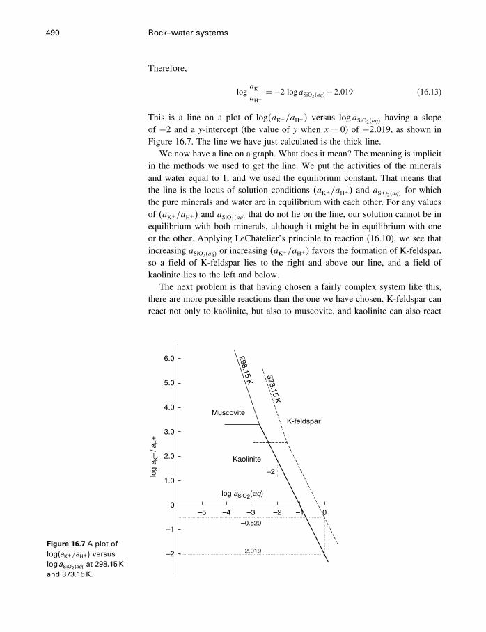
490 Rock–water systems
Therefore,
logaK+
aH+= −2 logaSiO2�aq�
−2�019 (16.13)
This is a line on a plot of log�aK+/aH+� versus logaSiO2�aq�having a slope
of −2 and a y-intercept (the value of y when x = 0) of −2�019, as shown inFigure 16.7. The line we have just calculated is the thick line.
We now have a line on a graph. What does it mean? The meaning is implicitin the methods we used to get the line. We put the activities of the mineralsand water equal to 1, and we used the equilibrium constant. That means thatthe line is the locus of solution conditions �aK+/aH+� and aSiO2�aq�
for whichthe pure minerals and water are in equilibrium with each other. For any valuesof �aK+/aH+� and aSiO2�aq�
that do not lie on the line, our solution cannot be inequilibrium with both minerals, although it might be in equilibrium with oneor the other. Applying LeChatelier’s principle to reaction (16.10), we see thatincreasing aSiO2�aq�
or increasing �aK+/aH+� favors the formation of K-feldspar,so a field of K-feldspar lies to the right and above our line, and a field ofkaolinite lies to the left and below.
The next problem is that having chosen a fairly complex system like this,there are more possible reactions than the one we have chosen. K-feldspar canreact not only to kaolinite, but also to muscovite, and kaolinite can also react
Figure 16.7 A plot oflog�aK+/aH+ � versuslogaSiO2�aq�
at 298.15 Kand 373.15 K.
6.0
5.0
4.0
3.0
2.0
1.0
0
–1
–2
–5 –4 –3 –2
–2
K-feldspar
–1 0
–2.019
–0.520
log aSiO2(aq)
log
a K+
/aH+
Kaolinite
Muscovite
298.15 K
373.15 K
16.5 Mineral stability diagrams 491
to form muscovite. These reactions are
32KAlSi3O8�s�+H+ = 1
2KAl3Si3O10�OH�2�s�+3SiO2�aq�+K+ (16.14)
and
KAl3Si3O10�OH�2�s�+ 32H2O+H+ = 3
2Al2Si2O5�OH�4�s�+K+ (16.15)
Using the same methods as before, we find that reaction (16.14) has a slopeof −3 on our graph, and an intercept (logK) of −4�668, and reaction (16.15)has a slope of 0 (it is independent of aSiO2
) and an intercept of 3�281. It can beshown (using the phase rule) that these three lines must intersect at a point, andso another way to draw them is to calculate the point of intersection, whichis logaSiO2�aq�
=−2�650, log�aK+/aH+�= 3�281, and draw lines with slopes 0,−2, and −3 through this point. We now have a kind of phase diagram, showingwhich minerals are stable, not as a function of T and P, but of the compositionof a solution in equilibrium with the minerals.
Effect of temperatureThere are other mineral phases to be added to our diagram, but first let’s lookat the effect of temperature. If we want the same diagram for a temperature of100 �C, we must calculate K at this temperature. To do this, we can use (9.20)or (9.22). We’ll use both in the following calculations. For reaction (16.10),�rH
� = 43437 Jmol−1 and �rS� = 106�449 Jmol−1/K. Therefore
�rG�373 = �rH
�298−T �rS�298
= 43437−373�15×106�449
= 3715�556 Jmol−1
logK =−3715�556/�2�30259×8�3145×373�15�
=−0�520
= logaK+
aH++2 logaSiO2�aq�
giving
logaK+
aH+= −2 logaSiO2�aq�
−0�520
as the equation of the K-feldspar–kaolinite boundary at 100 �C.
492 Rock–water systems
For reaction (16.14), �rH� = 74473 Jmol−1 and logK298 =−4�668, and so
logK373 = logK298−�rH
�298
2�30259R
(1T− 1
298�15
)=−4�668− 74473
2�30259×8�3145
(1
373�15− 1
298�15
)=−2�046
For reaction (16.15), �rH� = −18635 Jmol−1, �rS
� = −1�165 Jmol−1/K, andso
logK373 =−�rH
�298
2�30259RT+ �rS
�298
2�30259R
= 186352�30259×8�3145×373�15
+ −1�1652�30259×8�3145
= 2�548
These three lines intersect at log�aK+/aH+� = 2�55, logaSiO2�aq�= −1�53, as
shown in Figure 16.7.
Effect of choice of dataThis business of looking up data and plotting by hand gets tedious. Surelythere are computer programs to do all this for us? There are many, but none ofthem relieves the user of a fundamental responsibility – you are responsible forchoosing your data, and of course for understanding what you are doing. Peoplelearning how to use thermodynamics generally assume that the data they find atthe back of their text, such as those in Appendix B, are “true” in some absolutesense, and this does no harm while learning the subject. However, when youbegin to apply the subject in some area of interest, you sooner or later discoverthat there are a number of sources of data, that they often disagree, and thatthe choice of data can affect your results considerably.
One such source of data is supcrt92 (Johnson et al., 1992). In Figure 16.8are shown the mineral boundaries calculated using K values from supcrt92for 373.15K, in comparison with those from Figure 16.7. This comparisonis made to impress on you the fairly large differences that can result fromusing different sources of data. Most compilations of data these days have beensubjected to some sort of quality and consistency analysis, but methods vary.The refinement and improvement of thermodynamic data is a never-endingprocess, and the choice of thermodynamic data is an integral part of applyingthermodynamics to natural systems. The data in supcrt92 are especially goodfor most geochemical applications, because they have been derived using manyhigh pressure–temperature experiments involving minerals that are not alwaysconsidered by chemists. In other words, they are “tuned” to mineral equilibria.On the other hand, it does not contain many compounds that do not occur innature which are of great interest to chemists.

16.5 Mineral stability diagrams 493
The differences between the data in Appendix B and those in supcrt92 arerelatively small (Table 16.4), yet they result in quite large differences in phasediagrams like Figure 16.8. Let this be a lesson in choosing data – the best arenone too good, and no one knows for sure what “the best” data are.
While we are using supcrt92, we might as well add two final reactions toour diagram. These relate kaolinite and muscovite to gibbsite:
Al2Si2O5�OH�4�s�+H2O�l�= 2Al�OH�3�s�+2SiO2�aq� (16.16)
and
KAl3Si3O10�OH�2�s�+3H2O�l�+H+ = 3Al�OH�3�s�+3SiO2�aq�+K+ (16.17)
These two reactions also meet at a point with the muscovite–kaolinite reaction,as shown in Figure 16.8.
Table 16.4 The difference between the data in Appendix B and in supcrt92.
supcrt92 Appendix B App. B – supcrt92
Mineral �fG�, kJmol−1 �fG
�, kJmol−1 kJmol−1 % Difference
albite −3708�313 −3711�5 −3�2 0.08
K-feldspar −3746�245 −3742�9 −3�3 0.08
muscovite −5591�083 −5608�4 −17�3 0.30
quartz −856�239 −856�64 −0�4 0.05
SU
PC
RT9 2
0–1–2–3–4–5log aSiO2(aq)
1.0
2.0
3.0
4.0
5.0
6.0
log
a K+
/aH+
Gibbsite
Kaolinite
K-feldspar
Muscovite
Appendix B
373.15 K
Figure 16.8 A plot oflog�aK+/aH+ � versuslogaSiO2�aq�
at 373.15 K,showing the effect ofchanging from the data inAppendix B to data inprogram supcrt92.

494 Rock–water systems
The use of program supcrt92 is of no fundamental importance here. Wecould have illustrated the point that the choice of data is important by usingdata from any number of other sources.
The problem of metastable phasesOne of the pitfalls in choosing data and drawing diagrams, such as we havedone, is that we may not have considered all the possible reactions in oursystem. That is, there may be phases that are more stable than the ones wehave chosen – we may have chosen metastable phases. This is illustrated inour system by the fact that there is another aluminosilicate phase, pyrophyllite,which has more silica in it than does kaolinite and so is stable at higher valuesof aSiO2�aq�
. Considering the reactions
KAlSi3O8�s�+H+ = 12 Al2Si4O10�OH�2�s�+SiO2�aq�+K+ (16.18)
and
12Al2Si4O10�OH�2+ 1
2H2O�l�= 12Al2Si2O5�OH�4�s�+SiO2�aq� (16.19)
results in the two boundaries shown in Figure 16.9, which completely enclosethe K-feldspar–kaolinite boundary. This means that at 100 �C, and accordingto the supcrt92 data, K-feldspar and kaolinite are not stable together in the
Figure 16.9 A plot oflog�aK+/aH+ � versuslogaSiO2�aq�
at 373.15 K,using data from supcrt92,showing the stability fieldof pyrophyllite and thequartz saturation line.Each black squarerepresents a brine fromthe Kettleman NorthDome oil field (Merino,1975).
6.0
5.0
4.0
3.0
2.0
1.0
log
a K+
/aH
+
–5 –4 –3 –2 –1 0
Gibbsite
Muscovite
Supcrt92 Data
373.15 K
Qua
rtz
satu
ratio
n
K-feldspar
Pyrophyllite
K-feldspar
Kaolinite
Kaolinite
log aSiO2(aq)
16.5 Mineral stability diagrams 495
presence of water. They should react to form pyrophyllite. In nature, of course,they may not. K-feldspar may well react directly to kaolinite, in spite ofthermodynamics, but it would be a metastable reaction; that is, a reactioninvolving metastable phases.
One other thing. The solubility of quartz, calculated by the method in §9.4.1,is 10−3�078m at 100 �C according to supcrt92. This is shown in Figure 16.9as a vertical line. A solution in equilibrium with quartz at 100 �C must lieon this line. Solutions to the right of it are supersaturated, and solutions tothe left are undersaturated, with quartz. Therefore, if your system containsquartz, as most soils do, then not only is the assemblage K-feldspar + kaolinitemetastable with respect to pyrophyllite, but pyrophyllite is itself metastable.According to our diagram, pyrophyllite can only exist in an aqueous solutionif that solution is supersaturated with silica. If the silica were to precipitateas quartz, pyrophyllite should break down to form kaolinite, releasing silicato the solution, by reaction (16.19). Again, nature may not do this. It is quitecommon for natural solutions to be supersaturated with silica, even in thepresence of quartz, which is one reason that we use logaSiO2�aq�
as a variablein our diagrams.
Plotting solution dataAlso shown on Figure 16.9 are a few data points taken at random from Merino(1975). Each one is from a different well in the Kettleman North Dome oil fieldin California. The numbers for aK+ , aH+ , and aSiO2�aq�
are obtained from thechemical analyses in Merino (1975) by speciation. It appears that the solutionconcentrations are clustering around the K-feldspar–muscovite boundary, nearthe quartz saturation line, and are likely being controlled by these phases, whichare known to be in the sandstones containing the fluids sampled.
The albite–K-feldspar diagramThere are, of course, a great many diagrams we might plot, depending onour interests. To investigate the possibility that the K/Na ratio in the fluidsat Kettleman North Dome is controlled by the coexistence of albite andK-feldspar, we could write and plot the reaction
NaAlSi3O8�s�+K+ = KAlSi3O8�s�+Na+ (16.20)
Following the procedures outlined above, we find that �rG�373 =
−7052�9 Jmol−1 (Appendix B) or −14945 Jmol−1 (supcrt92). If pure albiteand pure K-feldspar are present in the rocks, the equilibrium constant for thisreaction becomes
K373 =aNa+
aK+(16.21)
= 100�987 Appendix B
or = 102�092 supcrt92
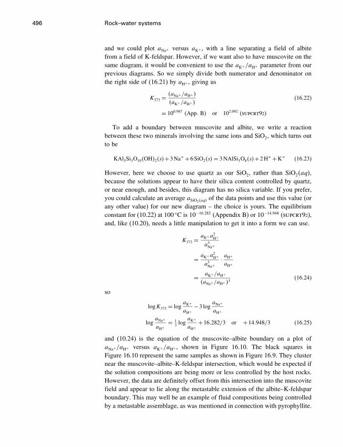
496 Rock–water systems
and we could plot aNa+ versus aK+ , with a line separating a field of albitefrom a field of K-feldspar. However, if we want also to have muscovite on thesame diagram, it would be convenient to use the aK+/aH+ parameter from ourprevious diagrams. So we simply divide both numerator and denominator onthe right side of (16.21) by aH+ , giving us
K373 =�aNa+/aH+�
�aK+/aH+�(16.22)
= 100�987 �App� B� or 102�092 (supcrt92)
To add a boundary between muscovite and albite, we write a reactionbetween these two minerals involving the same ions and SiO2, which turns outto be
KAl3Si3O10�OH�2�s�+3Na++6SiO2�s�= 3NAlSi3O8�s�+2H++K+ (16.23)
However, here we choose to use quartz as our SiO2, rather than SiO2�aq�,because the solutions appear to have their silica content controlled by quartz,or near enough, and besides, this diagram has no silica variable. If you prefer,you could calculate an average aSiO2�aq�
of the data points and use this value (orany other value) for our new diagram – the choice is yours. The equilibriumconstant for (10.22) at 100 �C is 10−16�282 (Appendix B) or 10−14�948 (supcrt92),and, like (10.20), needs a little manipulation to get it into a form we can use.
K373 =aK+a2H+
a3Na+
= aK+a2H+
a3Na+· aH+
aH+
= aK+/aH+
�aNa+/aH+�3(16.24)
so
logK373 = logaK+
aH+−3 log
aNa+
aH+
logaNa+
aH+= 1
3 logaK+
aH++16�282/3 or +14�948/3 (16.25)
and (10.24) is the equation of the muscovite–albite boundary on a plot ofaNa+/aH+ versus aK+/aH+ , shown in Figure 16.10. The black squares inFigure 16.10 represent the same samples as shown in Figure 16.9. They clusternear the muscovite–albite–K-feldspar intersection, which would be expected ifthe solution compositions are being more or less controlled by the host rocks.However, the data are definitely offset from this intersection into the muscovitefield and appear to lie along the metastable extension of the albite–K-feldsparboundary. This may well be an example of fluid compositions being controlledby a metastable assemblage, as was mentioned in connection with pyrophyllite.
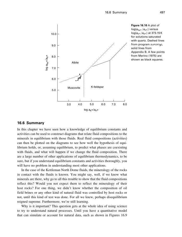
16.6 Summary 497
10.0
9.0
8.0
7.0
6.0
5.0
Albite
Muscovite K-feldspar
log
a Na+
/aH+
log aK+/aH+
3.0 4.0 5.0 6.0 7.0 8.0
Figure 16.10 A plot oflog�aNa+/aH+ � versuslog�aK+/aH+ � at 373.15 Kfor solutions saturatedwith quartz. Dashed linesfrom program supcrt92,solid lines fromAppendix B. A few pointsfrom Merino (1975) areshown as black squares.
16.6 Summary
In this chapter we have seen how a knowledge of equilibrium constants andactivities can be used to construct diagrams that relate fluid compositions to theminerals in equilibrium with those fluids. Real fluid compositions (activities)can then be plotted on the diagrams to see how well the hypothesis of equi-librium holds, or, assuming equilibrium, to predict what phases are coexistingwith fluids, and what will happen if we change the fluid composition. Thereare a large number of other applications of equilibrium thermodynamics, to besure, but if you understand equilibrium constants and activities thoroughly, youwill have no problem in understanding most other applications.
In the case of the Kettleman North Dome fluids, the mineralogy of the rocksin contact with the fluids is known. You might say, well, if we know whatminerals are there, why go to all this trouble to show that the fluid compositionsreflect this? Would you not expect them to reflect the mineralogy of theirhost rocks? For one thing, we didn’t know whether the composition of oilfield brines or any other kind of natural fluid was controlled by host rocks ornot, until this kind of test was done. For all we knew, perhaps disequilibriumreigned supreme. Furthermore, we’re still learning.
Why is it important? This question gets at the whole idea of using scienceto try to understand natural processes. Until you have a quantitative modelthat can simulate or account for natural data, such as shown in Figures 16.9

498 Rock–water systems
and 16.10, you cannot hope to change or control the situation to your benefit.For example, the petroleum geologists at Kettleman North Dome might want toinject something to change the fluid characteristics. Without a chemical model,they would have no way of predicting what would happen. The equilibriummodel has its limitations, but it is a good place to start.
17Phase diagrams
17.1 What is a phase diagram?
A phase diagram in the general sense is any diagram that shows what phaseor phases are stable as a function of some chosen system variable or variables.Therefore, the Eh–pH, logfO2
–pH and activity–activity diagrams we have beenlooking at are a kind of phase diagram. However, if you mention the subject ofphase diagrams to a petrologist, a metallurgist, or a ceramic scientist, they willimmediately think of a particular type of diagram that is of great usefulnessin these subjects. In these sciences, the compositions of phases and their rela-tionships during phase changes, particularly solid→liquid and liquid→solidchanges, are of particular importance, so diagrams that depict this informationas a function of temperature and pressure have come to be the subject of “phasediagrams.”
17.1.1 Thermodynamics and phase diagrams
Though it is true that phase relations can always be described in terms ofthe thermodynamic principles and equations we have been discussing, andthat any phase diagram can in principle be calculated given the appropriatedata, the emphasis in this chapter changes from one of calculating what wewant to know from numbers in tables of data, to one of simply representingexperimentally derived facts in diagrammatic form. The reason for this is thatonce we get into systems more complex than a single component, and especiallywhen high-temperature melt phases are involved, the calculations are often notpossible because the data are not available, and even if they are available, arenot very accurate, because they are very sensitive to small inaccuracies in thedata. Therefore, in this book, although we will show the relationship betweenfunctions such as G and our diagrams, this will be in an illustrative rather thana quantitative way.
17.1.2 Phase diagrams as models
Metallurgists and ceramicists quite often deal with simple two- and three-component systems and use phase diagrams to represent their experimental
499
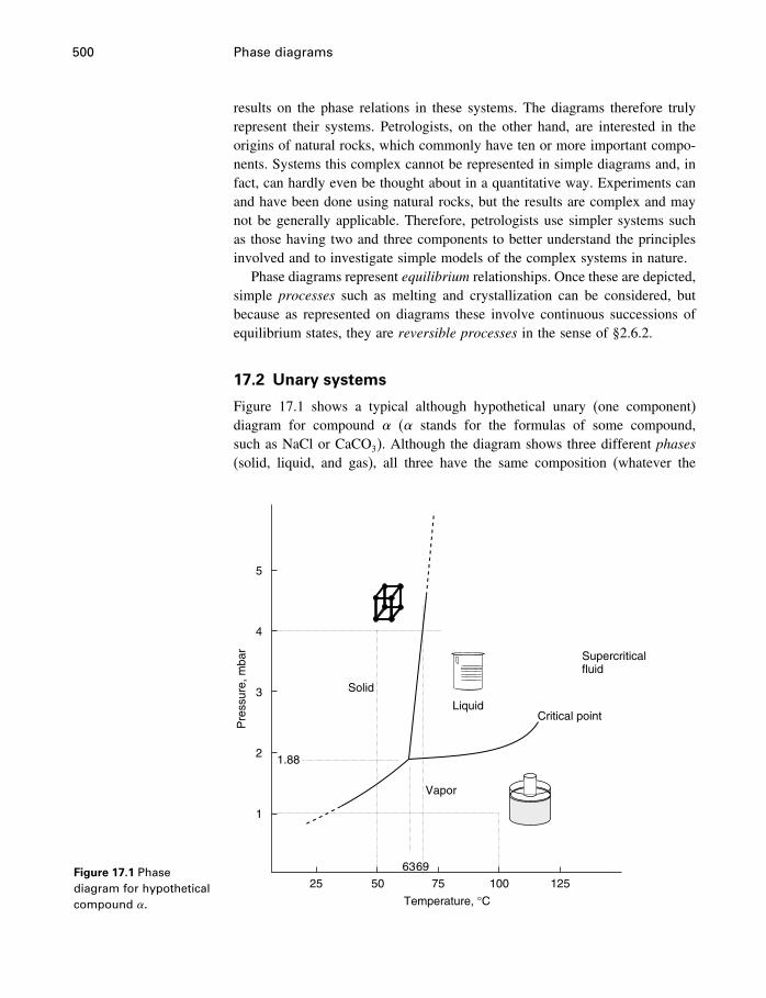
500 Phase diagrams
results on the phase relations in these systems. The diagrams therefore trulyrepresent their systems. Petrologists, on the other hand, are interested in theorigins of natural rocks, which commonly have ten or more important compo-nents. Systems this complex cannot be represented in simple diagrams and, infact, can hardly even be thought about in a quantitative way. Experiments canand have been done using natural rocks, but the results are complex and maynot be generally applicable. Therefore, petrologists use simpler systems suchas those having two and three components to better understand the principlesinvolved and to investigate simple models of the complex systems in nature.
Phase diagrams represent equilibrium relationships. Once these are depicted,simple processes such as melting and crystallization can be considered, butbecause as represented on diagrams these involve continuous successions ofequilibrium states, they are reversible processes in the sense of §2.6.2.
17.2 Unary systems
Figure 17.1 shows a typical although hypothetical unary (one component)diagram for compound ( stands for the formulas of some compound,such as NaCl or CaCO3). Although the diagram shows three different phases(solid, liquid, and gas), all three have the same composition (whatever the
Figure 17.1 Phasediagram for hypotheticalcompound �. Temperature, °C
Critical pointLiquid
Solid
1.88
6369
Vapor
Supercriticalfluid
Pre
ssur
e, m
bar
25
1
2
3
4
5
50 75 100 125
17.2 Unary systems 501
chemical composition of is), and so the system is unary. This simple diagramcontains a surprising amount of information, but you must know how to “read”the diagram. First, note that the diagram contains labeled areas, lines thatseparate the areas, and points. Every location on the diagram has a pair ofx–y coordinates, that is, a pressure and a temperature. For example, a pressureof 4mbar and a temperature of 50 �C are the coordinates of a point in thearea marked Solid. Under these conditions, the stable form of compound isobserved to be a crystalline solid. If the pressure on is reduced to 1mbar, andthe temperature increased to 100 �C, the stable form of is gaseous. Similarly,for any combination of pressures and temperatures within the area markedLiquid, the stable form of is liquid. The phase diagram is in fact a record ofthese experimental observations about the form of under various conditionsof P and T . As mentioned earlier, the vast majority of phase diagrams recordthe results of experiments – they are not usually the result of theoreticalcalculations. They are more often a source of thermodynamic data than theresult of using such data.
Obviously, within these areas, P and T could be changed considerablywithout changing the nature of the phase, although the properties of the phase(its density or heat capacity, say) would certainly change with P and T . Itappears, then, that for , and for any pure compound, we must choose twovariables in order to define the state of the compound. Thus to answer thequestion “what is the density (or heat capacity, refractive index, entropy,…) of?” we must first specify two variables – the P and the T we are interestedin. One is not enough – at 4mbar, can have quite a range of densities,but at 4mbar, 50 �C, its density is fixed and determinable, as are all its otherproperties. So we say that in each of its three forms – solid, liquid, and gas – has two degrees of freedom – two variables must be specified before all arespecified. These two variables are in practice usually T and P, but in principleany two would do. The phase rule summarizes all this discussion by simplysaying
f = c−p+2
= 1−1+2
= 2
With at 4mbar and 50 �C, consider that we raise the temperature gradually.Nothing much happens, except that the properties of change continuously,until we reach 69 �C, which is the temperature of the boundary between thesolid and liquid fields. At this T , solid is observed to begin to melt, and atthis T , any proportions of solid and liquid are possible (i.e., almost all solid with a drop of liquid; or almost all liquid with a tiny amount of solid; oranything in between). However, if the temperature is held very slightly abovethe melting T , becomes completely liquid. The solid–liquid boundary line
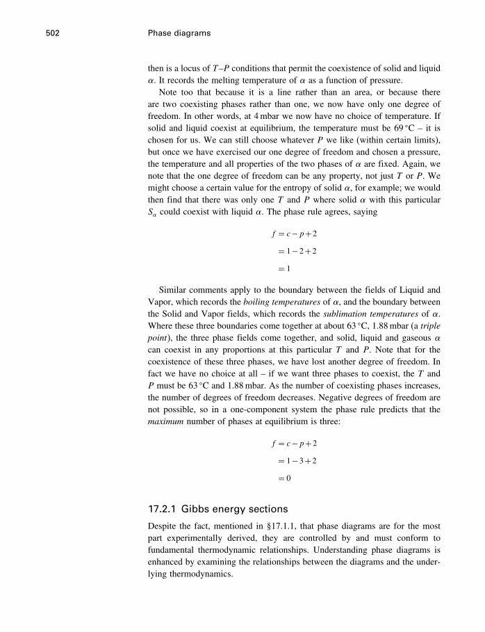
502 Phase diagrams
then is a locus of T–P conditions that permit the coexistence of solid and liquid. It records the melting temperature of as a function of pressure.
Note too that because it is a line rather than an area, or because thereare two coexisting phases rather than one, we now have only one degree offreedom. In other words, at 4mbar we now have no choice of temperature. Ifsolid and liquid coexist at equilibrium, the temperature must be 69 �C – it ischosen for us. We can still choose whatever P we like (within certain limits),but once we have exercised our one degree of freedom and chosen a pressure,the temperature and all properties of the two phases of are fixed. Again, wenote that the one degree of freedom can be any property, not just T or P. Wemight choose a certain value for the entropy of solid , for example; we wouldthen find that there was only one T and P where solid with this particularS could coexist with liquid . The phase rule agrees, saying
f = c−p+2
= 1−2+2
= 1
Similar comments apply to the boundary between the fields of Liquid andVapor, which records the boiling temperatures of , and the boundary betweenthe Solid and Vapor fields, which records the sublimation temperatures of .Where these three boundaries come together at about 63 �C, 1.88mbar (a triplepoint), the three phase fields come together, and solid, liquid and gaseous can coexist in any proportions at this particular T and P. Note that for thecoexistence of these three phases, we have lost another degree of freedom. Infact we have no choice at all – if we want three phases to coexist, the T andP must be 63 �C and 1.88mbar. As the number of coexisting phases increases,the number of degrees of freedom decreases. Negative degrees of freedom arenot possible, so in a one-component system the phase rule predicts that themaximum number of phases at equilibrium is three:
f = c−p+2
= 1−3+2
= 0
17.2.1 Gibbs energy sections
Despite the fact, mentioned in §17.1.1, that phase diagrams are for the mostpart experimentally derived, they are controlled by and must conform tofundamental thermodynamic relationships. Understanding phase diagrams isenhanced by examining the relationships between the diagrams and the under-lying thermodynamics.
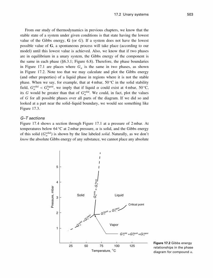
17.2 Unary systems 503
From our study of thermodynamics in previous chapters, we know that thestable state of a system under given conditions is that state having the lowestvalue of the Gibbs energy, G (or G). If a system does not have the lowestpossible value of G, a spontaneous process will take place (according to ourmodel) until this lowest value is achieved. Also, we know that if two phasesare in equilibrium in a unary system, the Gibbs energy of the component isthe same in each phase (§6.3.1; Figure 6.8). Therefore, the phase boundariesin Figure 17.1 are places where G is the same in two phases, as shownin Figure 17.2. Note too that we may calculate and plot the Gibbs energy(and other properties) of a liquid phase in regions where it is not the stablephase. When we say, for example, that at 4mbar, 50 �C in the solid stabilityfield, Gsolid
< Gliquid , we imply that if liquid could exist at 4mbar, 50 �C,
its G would be greater than that of Gsolid . We could, in fact, plot the values
of G for all possible phases over all parts of the diagram. If we did so andlooked at a part near the solid–liquid boundary, we would see something likeFigure 17.3.
G–T sectionsFigure 17.4 shows a section through Figure 17.1 at a pressure of 2mbar. Attemperatures below 64 �C at 2mbar pressure, is solid, and the Gibbs energyof this solid (Gsolid
) is shown by the line labeled solid. Naturally, as we don’tknow the absolute Gibbs energy of any substance, we cannot place any absolute
5
4
3
2
1
Temperature, °C
Pre
ssur
e, m
bar
25 50 75 100 125
Critical point
Liquid
αα
Gliquid = G
vapor
α
α
Gso
lid =Gva
por
Solid
Vapor
αα
Gso
lid =
Gliq
uid
G solid =G liquid =G vaporα α α
Figure 17.2 Gibbs energyrelationships in the phasediagram for compound �.
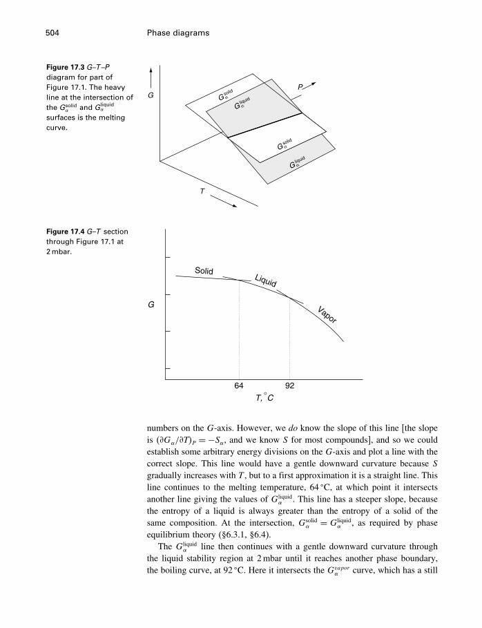
504 Phase diagrams
Figure 17.3 G–T –Pdiagram for part ofFigure 17.1. The heavyline at the intersection ofthe Gsolid
� and Gliquid�
surfaces is the meltingcurve.
G
T
P
Gsolid
Gliquidα
Gsolidα
α
Gliquid
α
Figure 17.4 G–T sectionthrough Figure 17.1 at2 mbar.
64 92
Solid
G
Liquid
Vapor
T, °C
numbers on the G-axis. However, we do know the slope of this line [the slopeis ��G/�T�P =−S, and we know S for most compounds], and so we couldestablish some arbitrary energy divisions on the G-axis and plot a line with thecorrect slope. This line would have a gentle downward curvature because Sgradually increases with T , but to a first approximation it is a straight line. Thisline continues to the melting temperature, 64 �C, at which point it intersectsanother line giving the values of Gliquid
. This line has a steeper slope, becausethe entropy of a liquid is always greater than the entropy of a solid of thesame composition. At the intersection, Gsolid
= Gliquid , as required by phase
equilibrium theory (§6.3.1, §6.4).The Gliquid
line then continues with a gentle downward curvature throughthe liquid stability region at 2mbar until it reaches another phase boundary,the boiling curve, at 92 �C. Here it intersects the Gvapor curve, which has a still
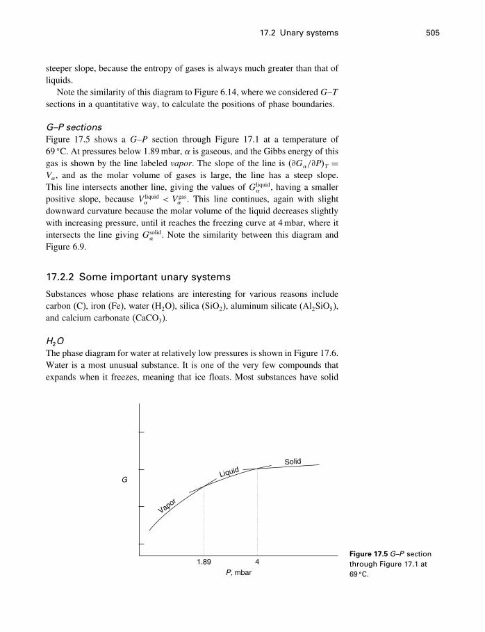
17.2 Unary systems 505
steeper slope, because the entropy of gases is always much greater than that ofliquids.
Note the similarity of this diagram to Figure 6.14, where we consideredG–Tsections in a quantitative way, to calculate the positions of phase boundaries.
G–P sectionsFigure 17.5 shows a G–P section through Figure 17.1 at a temperature of69 �C. At pressures below 1.89mbar, is gaseous, and the Gibbs energy of thisgas is shown by the line labeled vapor. The slope of the line is ��G/�P�T =V, and as the molar volume of gases is large, the line has a steep slope.This line intersects another line, giving the values of Gliquid
, having a smallerpositive slope, because V liquid
< V gas . This line continues, again with slight
downward curvature because the molar volume of the liquid decreases slightlywith increasing pressure, until it reaches the freezing curve at 4mbar, where itintersects the line giving Gsolid
. Note the similarity between this diagram andFigure 6.9.
17.2.2 Some important unary systems
Substances whose phase relations are interesting for various reasons includecarbon (C), iron (Fe), water (H2O), silica (SiO2), aluminum silicate (Al2SiO5),and calcium carbonate (CaCO3).
H2OThe phase diagram for water at relatively low pressures is shown in Figure 17.6.Water is a most unusual substance. It is one of the very few compounds thatexpands when it freezes, meaning that ice floats. Most substances have solid
Vapor
GLiquid
P, mbar
1.89 4
Solid
Figure 17.5 G–P sectionthrough Figure 17.1 at69 �C.
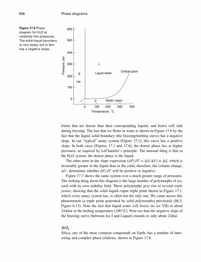
506 Phase diagrams
Figure 17.6 Phasediagram for H2O atrelatively low pressures.The solid–liquid boundaryis very steep, but in facthas a negative slope.
Temperature, °C
Liquid water
Water vapor
Critical point
L
V
S
Ice
Pre
ssur
e, b
ar
0
0
100
100
200
200
300
300
400
400
500
600
forms that are denser than their corresponding liquids, and hence will sinkduring freezing. The fact that ice floats in water is shown in Figure 17.6 by thefact that the liquid–solid boundary (the freezing/melting curve) has a negativeslope. In our “typical” unary system (Figure 17.1), this curve has a positiveslope. In both cases (Figures 17.1 and 17.6), the denser phase lies at higherpressures, as required by LeChatelier’s principle. The unusual thing is that inthe H2O system, the denser phase is the liquid.
The other term in the slope expression (dP/dT = �S/�V ) is �S, which isinvariably greater in the liquid than in the solid; therefore, the volume change,�V , determines whether dP/dT will be positive or negative.
Figure 17.7 shows the same system over a much greater range of pressures.The striking thing about this diagram is the large number of polymorphs of ice,each with its own stability field. These polymorphs give rise to several triplepoints, showing that the solid–liquid–vapor triple point shown in Figure 17.1,which every unary system has, is often not the only one. We came across thisphenomenon (a triple point generated by solid polymorphs) previously (§6.5,Figure 6.13). Note the fact that liquid water will freeze (to ice VII) at about24 kbar at the boiling temperature (100 �C). Note too that the negative slope ofthe freezing curve (between Ice I and Liquid) extends to only about 2 kbar.
SiO2
Silica, one of the most common compounds on Earth, has a number of inter-esting and complex phase relations, shown in Figure 17.8.
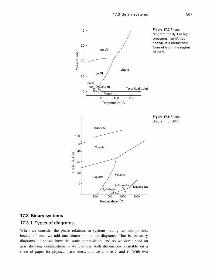
17.3 Binary systems 507
Temperature,°C0
0
10
20
30
40
100 200
Pre
ssur
e, k
bar
Liquid
Vapor
Ice VIce IIIIce II
Ice I
Ice VI
Ice VII
To critical point
Figure 17.7 Phasediagram for H2O at highpressures. Ice IV, notshown, is a metastableform of ice in the regionof Ice V.
Temperature, °C
Pre
ssur
e, k
bar
Liquid silica
Coesite
500 1000
10
20
30
40
160
20001500
Stishovite
α-quartzβ-quartz
β-Cristobalite
β2-Tridymite
Figure 17.8 Phasediagram for SiO2.
17.3 Binary systems
17.3.1 Types of diagrams
When we consider the phase relations in systems having two componentsinstead of one, we add one dimension to our diagrams. That is, in unarydiagrams all phases have the same composition, and so we don’t need anaxis showing compositions – we can use both dimensions available on asheet of paper for physical parameters, and we choose T and P. With two
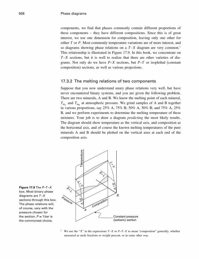
508 Phase diagrams
components, we find that phases commonly contain different proportions ofthese components – they have different compositions. Since this is of greatinterest, we use one dimension for composition, leaving only one other foreither T or P. Most commonly temperature variations are of more interest, andso diagrams showing phase relations on a T–X diagram are very common.1
This relationship is illustrated in Figure 17.9. In this book, we concentrate onT–X sections, but it is well to realize that there are other varieties of dia-grams. Not only do we have P–X sections, but P–T or isoplethal (constantcomposition) sections, as well as various projections.
17.3.2 The melting relations of two components
Suppose that you now understand unary phase relations very well, but havenever encountered binary systems, and you are given the following problem.There are two minerals, A and B. We know the melting point of each mineral,TmA
and TmBat atmospheric pressure. We grind samples of A and B together
in various proportions, say 25% A, 75% B; 50% A, 50% B; and 75% A, 25%B, and we perform experiments to determine the melting temperature of thesemixtures. Your job is to draw a diagram predicting the most likely results.The diagram should show temperature as the vertical axis, and composition asthe horizontal axis, and of course the known melting temperatures of the pureminerals A and B should be plotted on the vertical axes at each end of thecomposition axis.
Figure 17.9 The P –T –Xbox. Most binary phasediagrams are T –Xsections through this box.The phase relations will,of course, vary with thepressure chosen forthe section. P = 1 bar isthe commonest choice.
Constant pressure(isobaric) section
PressureComposition
Tem
pera
ture
A
B
S + L
S + L
S+
V
S+
V
L +V
L +V
1 We use the “X” in the expressions T–X or P–T–X to mean “composition” generally, whethermeasured as mole fractions or weight percent, or in some other way.
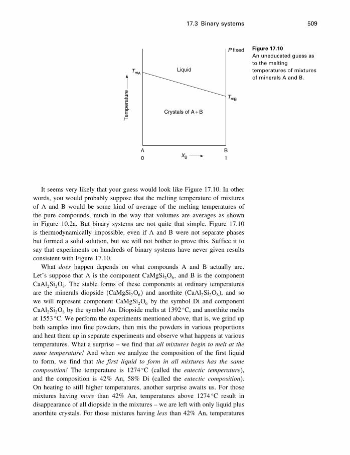
17.3 Binary systems 509
XB
A
Tem
pera
ture
Crystals of A + B
Liquid
P fixed
TmA
TmB
0 1B
Figure 17.10An uneducated guess asto the meltingtemperatures of mixturesof minerals A and B.
It seems very likely that your guess would look like Figure 17.10. In otherwords, you would probably suppose that the melting temperature of mixturesof A and B would be some kind of average of the melting temperatures ofthe pure compounds, much in the way that volumes are averages as shownin Figure 10.2a. But binary systems are not quite that simple. Figure 17.10is thermodynamically impossible, even if A and B were not separate phasesbut formed a solid solution, but we will not bother to prove this. Suffice it tosay that experiments on hundreds of binary systems have never given resultsconsistent with Figure 17.10.
What does happen depends on what compounds A and B actually are.Let’s suppose that A is the component CaMgSi2O6, and B is the componentCaAl2Si2O8. The stable forms of these components at ordinary temperaturesare the minerals diopside (CaMgSi2O6) and anorthite (CaAl2Si2O8), and sowe will represent component CaMgSi2O6 by the symbol Di and componentCaAl2Si2O8 by the symbol An. Diopside melts at 1392 �C, and anorthite meltsat 1553 �C. We perform the experiments mentioned above, that is, we grind upboth samples into fine powders, then mix the powders in various proportionsand heat them up in separate experiments and observe what happens at varioustemperatures. What a surprise – we find that all mixtures begin to melt at thesame temperature! And when we analyze the composition of the first liquidto form, we find that the first liquid to form in all mixtures has the samecomposition! The temperature is 1274 �C (called the eutectic temperature),and the composition is 42% An, 58% Di (called the eutectic composition).On heating to still higher temperatures, another surprise awaits us. For thosemixtures having more than 42% An, temperatures above 1274 �C result indisappearance of all diopside in the mixtures – we are left with only liquid plusanorthite crystals. For those mixtures having less than 42% An, temperatures
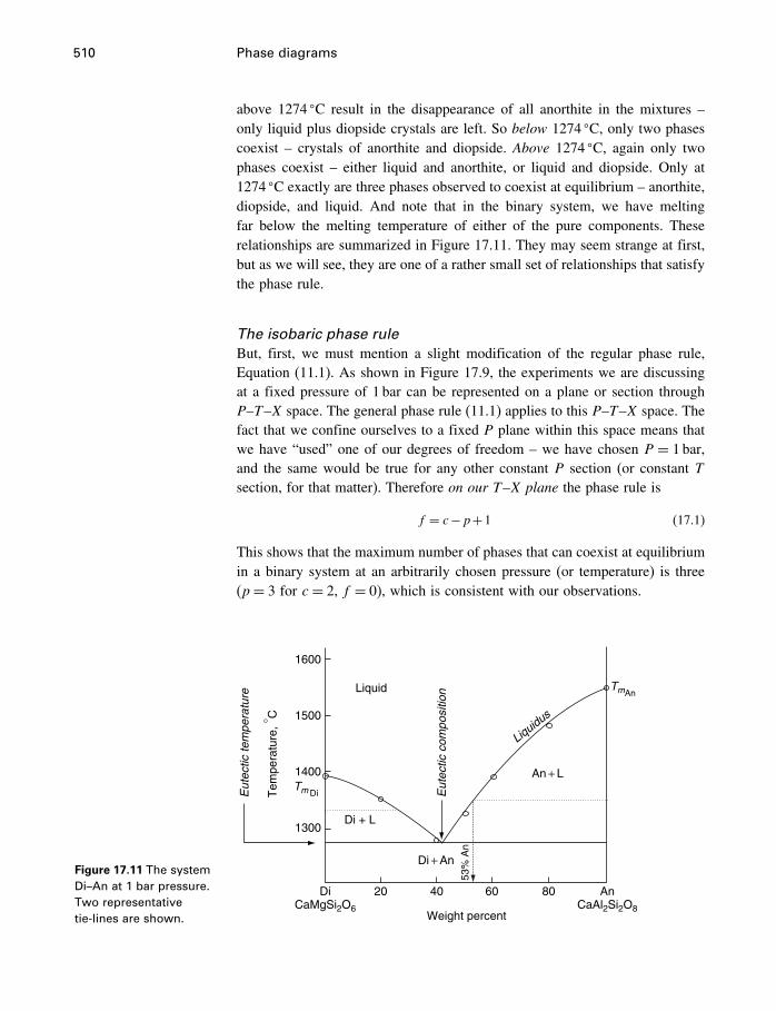
510 Phase diagrams
above 1274 �C result in the disappearance of all anorthite in the mixtures –only liquid plus diopside crystals are left. So below 1274 �C, only two phasescoexist – crystals of anorthite and diopside. Above 1274 �C, again only twophases coexist – either liquid and anorthite, or liquid and diopside. Only at1274 �C exactly are three phases observed to coexist at equilibrium – anorthite,diopside, and liquid. And note that in the binary system, we have meltingfar below the melting temperature of either of the pure components. Theserelationships are summarized in Figure 17.11. They may seem strange at first,but as we will see, they are one of a rather small set of relationships that satisfythe phase rule.
The isobaric phase ruleBut, first, we must mention a slight modification of the regular phase rule,Equation (11.1). As shown in Figure 17.9, the experiments we are discussingat a fixed pressure of 1 bar can be represented on a plane or section throughP–T–X space. The general phase rule (11.1) applies to this P–T–X space. Thefact that we confine ourselves to a fixed P plane within this space means thatwe have “used” one of our degrees of freedom – we have chosen P = 1 bar,and the same would be true for any other constant P section (or constant Tsection, for that matter). Therefore on our T–X plane the phase rule is
f = c−p+1 (17.1)
This shows that the maximum number of phases that can coexist at equilibriumin a binary system at an arbitrarily chosen pressure (or temperature) is three(p= 3 for c = 2, f = 0), which is consistent with our observations.
Figure 17.11 The systemDi–An at 1 bar pressure.Two representativetie-lines are shown.
DiCaMgSi2O6
Eut
ectic
tem
pera
ture
Eut
ectic
com
posi
tion
Tem
pera
ture
,°C
Weight percent
An + L
Di + L
Di + An
53%
An
Liquid
Liquidus
AnCaAl2Si2O8
1600
1500
1400
1300
Tm Di
TmAn
20 40 60 80
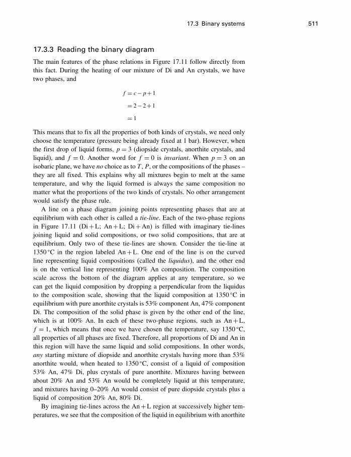
17.3 Binary systems 511
17.3.3 Reading the binary diagram
The main features of the phase relations in Figure 17.11 follow directly fromthis fact. During the heating of our mixture of Di and An crystals, we havetwo phases, and
f = c−p+1
= 2−2+1
= 1
This means that to fix all the properties of both kinds of crystals, we need onlychoose the temperature (pressure being already fixed at 1 bar). However, whenthe first drop of liquid forms, p = 3 (diopside crystals, anorthite crystals, andliquid), and f = 0. Another word for f = 0 is invariant. When p = 3 on anisobaric plane, we have no choice as to T , P, or the compositions of the phases –they are all fixed. This explains why all mixtures begin to melt at the sametemperature, and why the liquid formed is always the same composition nomatter what the proportions of the two kinds of crystals. No other arrangementwould satisfy the phase rule.
A line on a phase diagram joining points representing phases that are atequilibrium with each other is called a tie-line. Each of the two-phase regionsin Figure 17.11 (Di+L; An+L; Di+An) is filled with imaginary tie-linesjoining liquid and solid compositions, or two solid compositions, that are atequilibrium. Only two of these tie-lines are shown. Consider the tie-line at1350 �C in the region labeled An+L. One end of the line is on the curvedline representing liquid compositions (called the liquidus), and the other endis on the vertical line representing 100% An composition. The compositionscale across the bottom of the diagram applies at any temperature, so wecan get the liquid composition by dropping a perpendicular from the liquidusto the composition scale, showing that the liquid composition at 1350 �C inequilibrium with pure anorthite crystals is 53% component An, 47% componentDi. The composition of the solid phase is given by the other end of the line,which is at 100% An. In each of these two-phase regions, such as An+L,f = 1, which means that once we have chosen the temperature, say 1350 �C,all properties of all phases are fixed. Therefore, all proportions of Di and An inthis region will have the same liquid and solid compositions. In other words,any starting mixture of diopside and anorthite crystals having more than 53%anorthite would, when heated to 1350 �C, consist of a liquid of composition53% An, 47% Di, plus crystals of pure anorthite. Mixtures having betweenabout 20% An and 53% An would be completely liquid at this temperature,and mixtures having 0–20% An would consist of pure diopside crystals plus aliquid of composition 20% An, 80% Di.
By imagining tie-lines across the An+L region at successively higher tem-peratures, we see that the composition of the liquid in equilibrium with anorthite
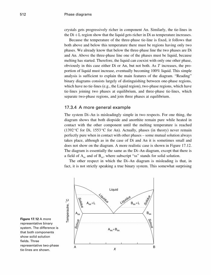
512 Phase diagrams
crystals gets progressively richer in component An. Similarly, the tie-lines inthe Di+L region show that the liquid gets richer in Di as temperature increases.
Because the temperature of the three-phase tie-line is fixed, it follows thatboth above and below this temperature there must be regions having only twophases. We already know that below the three-phase line the two phases are Diand An. Above the three-phase line one of the phases must be liquid, becausemelting has started. Therefore, the liquid can coexist with only one other phase,obviously in this case either Di or An, but not both. As T increases, the pro-portion of liquid must increase, eventually becoming 100% liquid. This simpleanalysis is sufficient to explain the main features of the diagram. “Reading”binary diagrams consists largely of distinguishing between one-phase regions,which have no tie-lines (e.g., the Liquid region), two-phase regions, which havetie-lines joining two phases at equilibrium, and three-phase tie-lines, whichseparate two-phase regions, and join three phases at equilibrium.
17.3.4 A more general example
The system Di–An is misleadingly simple in two respects. For one thing, thediagram shows that both diopside and anorthite remain pure while heated incontact with the other component until the melting temperature is reached(1392 �C for Di, 1553 �C for An). Actually, phases (in theory) never remainperfectly pure when in contact with other phases – some mutual solution alwaystakes place, although as in the case of Di and An it is sometimes small anddoes not show on the diagram. A more realistic case is shown in Figure 17.12.The diagram is essentially the same as the Di–An diagram, except that there isa field of Ass and of Bss, where subscript “ss” stands for solid solution.
The other respect in which the Di–An diagram is misleading is that, infact, it is not strictly speaking a true binary system. This somewhat surprising
Figure 17.12 A morerepresentative binarysystem. The difference isthat both componentsshow solid solutionfields. Threerepresentative two-phasetie-lines are shown. X
BA
Tem
pera
utre
,°C
Ass+Bss
Liquid
LiquidusLiquidus
Ass+L
Solidus
Sol
vus
Solvus
Sol
idus
Bss+L
Ass Bss
17.3 Binary systems 513
statement cannot be fully explained without discussing ternary systems. Sufficeit to say that just because you choose two components does not necessarilymean that you have a binary system. To be truly binary, all compositions of allphases must lie on the plane of the diagram. This must be the case in simplesystems such as Cu–Au and with single solution phases such as liquids; butwith complex components such as Di and An, although the bulk compositionmust lie on the plane of the diagram, the compositions of coexisting phasesmay each lie “off the plane” of the diagram. Careful work has shown that in thesystem Di–An, diopside crystals are not pure but contain some Al. This meansthat, because bulk compositions lie on the Di–An plane, phases coexisting withdiopside must be somewhat deficient in Al. To portray this in a diagram, oneneeds a three-component triangle. Just remember that not all choices of twocomponents are binary systems – some are planes within ternary systems.
Solid solutionsThere is no difference in principle between a solid solution and a liquid orgaseous solution. Substances dissolve into one another, like sugar into tea, orlike oxygen into nitrogen, because the Gibbs energy change of such a processis negative – they are spontaneous processes. Consider the system Di–An ata temperature of 1600 �C (Figure 17.11). At this temperature, both pure Diand pure An are liquid phases. If one gram of Di liquid and one gram ofAn liquid were mixed together, they would dissolve into one another to forma homogeneous liquid solution, represented by a point in the middle of thediagram on the 1600 �C isotherm. If pure diopside crystals are mixed with pureanorthite crystals at 1200 �C, on the other hand, nothing happens – they do notdissolve into each other.
Components A and B in Figure 17.12, on the other hand, behave differently.Liquid A and liquid B still mix to form a homogeneous solution, but when solidA and solid B are mixed together, they dissolve into one another to a limitedextent. Salt will dissolve into water, but not without limit – it will dissolve onlyuntil the water becomes saturated. Similarly, solid B will dissolve into solidA, but not without limit. It dissolves into A until A is saturated with B, and atthe same time A dissolves into B until B is saturated with A. The saturationlimits of each component in the other is shown by a line called the solvus. Theexistence of a solvus shows that A and B exhibit limited miscibility in the solidstate. They exhibit complete miscibility in the liquid state. “Miscibility” doesnot really mean “mixability,” although they sound similar. “Mixability,” if itis a word, just means things can be mixed together – mutual dissolution is notimplied. “Miscibility” means the ability to dissolve into something else.
Figure 17.12 shows a eutectic, but the two solid phases in equilibrium withthe liquid are not pure A and pure B; A contains some B in solid solution (Ass)and B contains some A in solid solution (Bss). Similarly, at temperatures abovethe eutectic, the liquid is not in equilibrium with pure A or pure B, but with
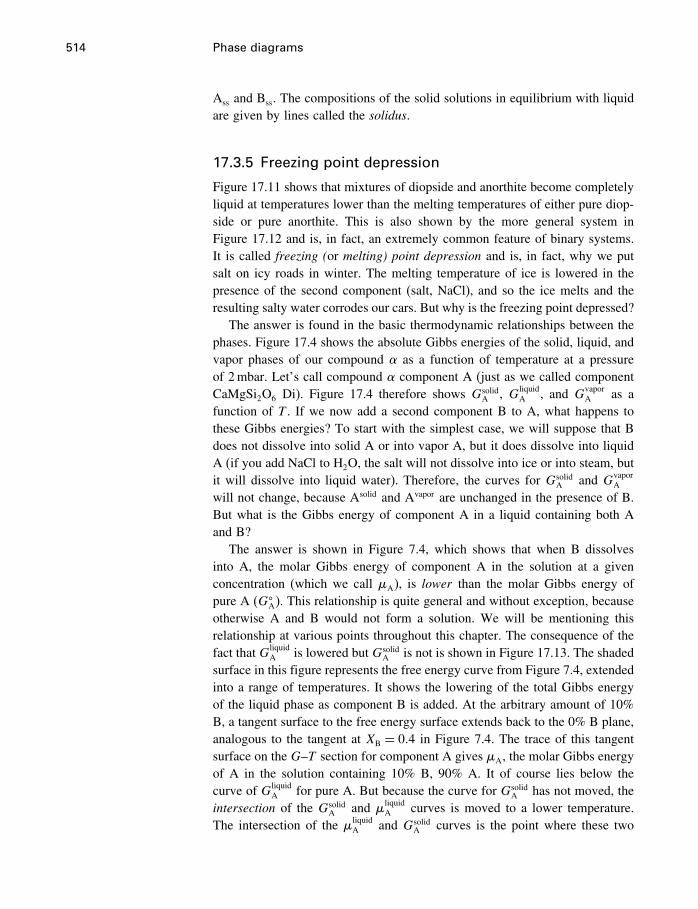
514 Phase diagrams
Ass and Bss. The compositions of the solid solutions in equilibrium with liquidare given by lines called the solidus.
17.3.5 Freezing point depression
Figure 17.11 shows that mixtures of diopside and anorthite become completelyliquid at temperatures lower than the melting temperatures of either pure diop-side or pure anorthite. This is also shown by the more general system inFigure 17.12 and is, in fact, an extremely common feature of binary systems.It is called freezing (or melting) point depression and is, in fact, why we putsalt on icy roads in winter. The melting temperature of ice is lowered in thepresence of the second component (salt, NaCl), and so the ice melts and theresulting salty water corrodes our cars. But why is the freezing point depressed?
The answer is found in the basic thermodynamic relationships between thephases. Figure 17.4 shows the absolute Gibbs energies of the solid, liquid, andvapor phases of our compound as a function of temperature at a pressureof 2mbar. Let’s call compound component A (just as we called componentCaMgSi2O6 Di). Figure 17.4 therefore shows Gsolid
A , GliquidA , and Gvapor
A as afunction of T . If we now add a second component B to A, what happens tothese Gibbs energies? To start with the simplest case, we will suppose that Bdoes not dissolve into solid A or into vapor A, but it does dissolve into liquidA (if you add NaCl to H2O, the salt will not dissolve into ice or into steam, butit will dissolve into liquid water). Therefore, the curves for Gsolid
A and GvaporA
will not change, because Asolid and Avapor are unchanged in the presence of B.But what is the Gibbs energy of component A in a liquid containing both Aand B?
The answer is shown in Figure 7.4, which shows that when B dissolvesinto A, the molar Gibbs energy of component A in the solution at a givenconcentration (which we call �A), is lower than the molar Gibbs energy ofpure A (G�
A). This relationship is quite general and without exception, becauseotherwise A and B would not form a solution. We will be mentioning thisrelationship at various points throughout this chapter. The consequence of thefact that Gliquid
A is lowered but GsolidA is not is shown in Figure 17.13. The shaded
surface in this figure represents the free energy curve from Figure 7.4, extendedinto a range of temperatures. It shows the lowering of the total Gibbs energyof the liquid phase as component B is added. At the arbitrary amount of 10%B, a tangent surface to the free energy surface extends back to the 0% B plane,analogous to the tangent at XB = 0�4 in Figure 7.4. The trace of this tangentsurface on the G–T section for component A gives �A, the molar Gibbs energyof A in the solution containing 10% B, 90% A. It of course lies below thecurve of Gliquid
A for pure A. But because the curve for GsolidA has not moved, the
intersection of the GsolidA and �liquid
A curves is moved to a lower temperature.The intersection of the �liquid
A and GsolidA curves is the point where these two
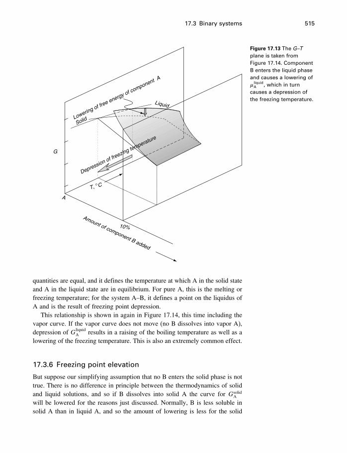
17.3 Binary systems 515
A
Amount of component B added
10%
G
Lowering of free energy of component A
Solid
T, °C
Liquid
Depression of freezing temperature
Figure 17.13 The G–Tplane is taken fromFigure 17.14. ComponentB enters the liquid phaseand causes a lowering of�
liquidA , which in turn
causes a depression ofthe freezing temperature.
quantities are equal, and it defines the temperature at which A in the solid stateand A in the liquid state are in equilibrium. For pure A, this is the melting orfreezing temperature; for the system A–B, it defines a point on the liquidus ofA and is the result of freezing point depression.
This relationship is shown in again in Figure 17.14, this time including thevapor curve. If the vapor curve does not move (no B dissolves into vapor A),depression of Gliquid
A results in a raising of the boiling temperature as well as alowering of the freezing temperature. This is also an extremely common effect.
17.3.6 Freezing point elevation
But suppose our simplifying assumption that no B enters the solid phase is nottrue. There is no difference in principle between the thermodynamics of solidand liquid solutions, and so if B dissolves into solid A the curve for Gsolid
A
will be lowered for the reasons just discussed. Normally, B is less soluble insolid A than in liquid A, and so the amount of lowering is less for the solid
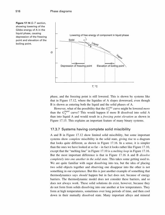
516 Phase diagrams
Figure 17.14 G–T section,showing lowering of theGibbs energy of A in theliquid phase, causingdepression of the freezingpoint and elevation of theboiling point.
T, °C
G
Lowering of free energy of component in liquid phase
Depression of freezing point Elevation of boiling point
Liquid
Vapor
Solid
phase, and the freezing point is still lowered. This is shown by systems likethat in Figure 17.12, where the liquidus of A slopes downward, even thoughB is shown as entering both the liquid and the solid phases of A.
However, what of the possibility that the GsolidA curve might be lowered more
than the GliquidA curve? This would happen if more B dissolved into solid A
than into liquid A and would result in a freezing point elevation as shown inFigure 17.15. This explains an important feature of many binary systems.
17.3.7 Systems having complete solid miscibility
A and B in Figure 17.12 show limited solid miscibility, but some importantsystems show complete miscibility in the solid state, giving rise to a diagramthat looks quite different, as shown in Figure 17.16. In a sense, it is simplerthan the ones we have looked at so far – in fact it looks rather like Figure 17.10,except that the “melting line” in Figure 17.10 is a melting loop in Figure 17.16.But the most important difference is that in Figure 17.16 A and B dissolvecompletely into one another in the solid state. This takes some getting used to.We are quite familiar with sugar dissolving into tea, but the idea of placingtwo solid objects together and observing one disappear into the other is notsomething in our experience. But this is just another example of something thatthermodynamics says should happen but in fact does not, because of energybarriers. The thermodynamic model does not consider these barriers, and sodoes not always work. These solid solutions do exist, however, because theydo not form from solids dissolving into one another at low temperatures. Theyform at high temperatures, sometimes over long periods of time, and then cooldown in their mutually dissolved state. Many important alloys and mineral
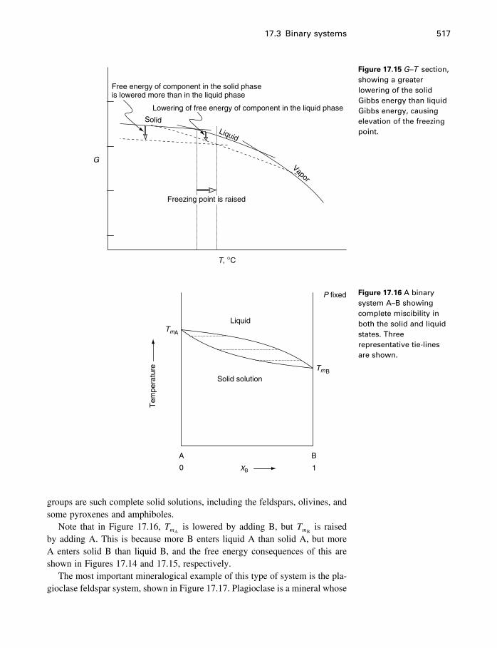
17.3 Binary systems 517
G
Free energy of component in the solid phase is lowered more than in the liquid phase
Lowering of free energy of component in the liquid phase
Freezing point is raised
SolidLiquid
Vapor
T, °C
Figure 17.15 G–T section,showing a greaterlowering of the solidGibbs energy than liquidGibbs energy, causingelevation of the freezingpoint.
Tem
pera
ture
Solid solution
TmA
TmB
Liquid
P fixed
XB
B
10
A
Figure 17.16 A binarysystem A–B showingcomplete miscibility inboth the solid and liquidstates. Threerepresentative tie-linesare shown.
groups are such complete solid solutions, including the feldspars, olivines, andsome pyroxenes and amphiboles.
Note that in Figure 17.16, TmAis lowered by adding B, but TmB
is raisedby adding A. This is because more B enters liquid A than solid A, but moreA enters solid B than liquid B, and the free energy consequences of this areshown in Figures 17.14 and 17.15, respectively.
The most important mineralogical example of this type of system is the pla-gioclase feldspar system, shown in Figure 17.17. Plagioclase is a mineral whose
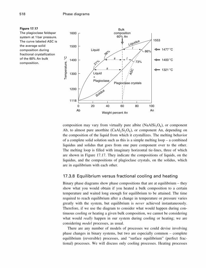
518 Phase diagrams
Figure 17.17The plagioclase feldsparsystem at 1 bar pressure.The curve labeled ASC isthe average solidcomposition duringfractional crystallizationof the 60% An bulkcomposition.
1600
86%
73%
36%
21%
1553
1500
Tem
pera
ture
,°C
1400 °C
1321 °C
1477 °C
1300
1400
1200
1118
200Ab
40 60 80 100An
Weight percent An
AS
C
Liquid+Plagioclase
Plagioclase crystals
Liquid
Solidus
Liquidus
Bulkcomposition
60% An
s
s l
l
composition may vary from virtually pure albite (NaAlSi3O8), or componentAb, to almost pure anorthite (CaAl2Si2O8), or component An, depending onthe composition of the liquid from which it crystallizes. The melting behaviorof a complete solid solution such as this is a simple melting loop – a combinedliquidus and solidus that goes from one pure component over to the other.The melting loop is filled with imaginary horizontal tie-lines, three of whichare shown in Figure 17.17. They indicate the compositions of liquids, on theliquidus, and the compositions of plagioclase crystals, on the solidus, whichare in equilibrium with each other.
17.3.8 Equilibrium versus fractional cooling and heating
Binary phase diagrams show phase compositions that are at equilibrium – theyshow what you would obtain if you heated a bulk composition to a certaintemperature and waited long enough for equilibrium to be attained. The timerequired to reach equilibrium after a change in temperature or pressure variesgreatly with the system, but equilibrium is never achieved instantaneously.Therefore, if we use the diagram to consider what would happen during con-tinuous cooling or heating a given bulk composition, we cannot be consideringwhat would really happen in our system during cooling or heating; we areconsidering model processes, as usual.
There are any number of models of processes we could devise involvingphase changes in binary systems, but two are especially common – completeequilibrium (reversible) processes, and “surface equilibrium” (perfect frac-tional) processes. We will discuss only cooling processes. Heating processes
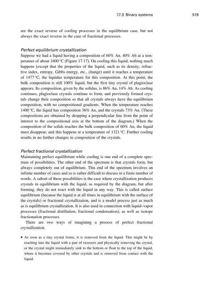
17.3 Binary systems 519
are the exact reverse of cooling processes in the equilibrium case, but notalways the exact reverse in the case of fractional processes.
Perfect equilibrium crystallizationSuppose we had a liquid having a composition of 60% An, 40% Ab at a tem-perature of about 1600 �C (Figure 17.17). On cooling this liquid, nothing muchhappens (except that the properties of the liquid, such as its density, refrac-tive index, entropy, Gibbs energy, etc., change) until it reaches a temperatureof 1477 �C, the liquidus temperature for this composition. At this point, thebulk composition is still 100% liquid, but the first tiny crystal of plagioclaseappears. Its composition, given by the solidus, is 86% An, 14% Ab. As coolingcontinues, plagioclase crystals continue to form, and previously formed crys-tals change their composition so that all crystals always have the equilibriumcomposition, with no compositional gradients. When the temperature reaches1400 �C, the liquid has composition 36% An, and the crystals 73% An. (Thesecompositions are obtained by dropping a perpendicular line from the point ofinterest to the compositional axis at the bottom of the diagram.) When thecomposition of the solids reaches the bulk composition of 60% An, the liquidmust disappear, and this happens at a temperature of 1321 �C. Further coolingresults in no further changes in composition of the crystals.
Perfect fractional crystallizationMaintaining perfect equilibrium while cooling is one end of a complete spec-trum of possibilities. The other end of the spectrum is that crystals form, butalways completely out of equilibrium. This end of the spectrum involves aninfinite number of cases and so is rather difficult to discuss in a finite number ofwords. A subset of these possibilities is the case where crystallization producescrystals in equilibrium with the liquid, as required by the diagram, but afterforming, they do not react with the liquid in any way. This is called surfaceequilibrium (because the liquid is at all times in equilibrium with the surface ofthe crystals) or fractional crystallization, and is a model process just as muchas is equilibrium crystallization. It is also used in connection with liquid–vaporprocesses (fractional distillation; fractional condensation), as well as isotopefractionation processes.
There are two ways of imagining a process of perfect fractionalcrystallization.
• As soon as a tiny crystal forms, it is removed from the liquid. This might be by
reaching into the liquid with a pair of tweezers and physically removing the crystal,
or the crystal might immediately sink to the bottom or float to the top of the liquid,
where it becomes covered by other crystals and is removed from contact with the
liquid.
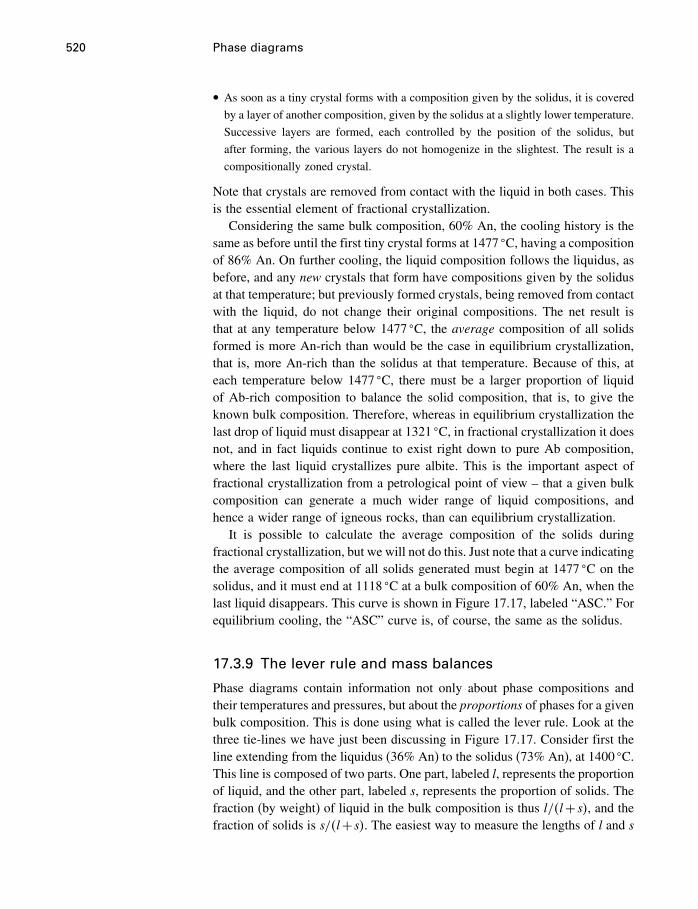
520 Phase diagrams
• As soon as a tiny crystal forms with a composition given by the solidus, it is covered
by a layer of another composition, given by the solidus at a slightly lower temperature.
Successive layers are formed, each controlled by the position of the solidus, but
after forming, the various layers do not homogenize in the slightest. The result is a
compositionally zoned crystal.
Note that crystals are removed from contact with the liquid in both cases. Thisis the essential element of fractional crystallization.
Considering the same bulk composition, 60% An, the cooling history is thesame as before until the first tiny crystal forms at 1477 �C, having a compositionof 86% An. On further cooling, the liquid composition follows the liquidus, asbefore, and any new crystals that form have compositions given by the solidusat that temperature; but previously formed crystals, being removed from contactwith the liquid, do not change their original compositions. The net result isthat at any temperature below 1477 �C, the average composition of all solidsformed is more An-rich than would be the case in equilibrium crystallization,that is, more An-rich than the solidus at that temperature. Because of this, ateach temperature below 1477 �C, there must be a larger proportion of liquidof Ab-rich composition to balance the solid composition, that is, to give theknown bulk composition. Therefore, whereas in equilibrium crystallization thelast drop of liquid must disappear at 1321 �C, in fractional crystallization it doesnot, and in fact liquids continue to exist right down to pure Ab composition,where the last liquid crystallizes pure albite. This is the important aspect offractional crystallization from a petrological point of view – that a given bulkcomposition can generate a much wider range of liquid compositions, andhence a wider range of igneous rocks, than can equilibrium crystallization.
It is possible to calculate the average composition of the solids duringfractional crystallization, but we will not do this. Just note that a curve indicatingthe average composition of all solids generated must begin at 1477 �C on thesolidus, and it must end at 1118 �C at a bulk composition of 60% An, when thelast liquid disappears. This curve is shown in Figure 17.17, labeled “ASC.” Forequilibrium cooling, the “ASC” curve is, of course, the same as the solidus.
17.3.9 The lever rule and mass balances
Phase diagrams contain information not only about phase compositions andtheir temperatures and pressures, but about the proportions of phases for a givenbulk composition. This is done using what is called the lever rule. Look at thethree tie-lines we have just been discussing in Figure 17.17. Consider first theline extending from the liquidus (36% An) to the solidus (73% An), at 1400 �C.This line is composed of two parts. One part, labeled l, represents the proportionof liquid, and the other part, labeled s, represents the proportion of solids. Thefraction (by weight) of liquid in the bulk composition is thus l/�l+ s�, and thefraction of solids is s/�l+ s�. The easiest way to measure the lengths of l and s
17.3 Binary systems 521
is probably by comparing the compositions of the end points of the tie-line atthe liquidus and solidus with the bulk composition. Thus the s portion of the tie-line has a length of 60−36= 24%, and the l portion of the tie-line has a lengthof 73−60= 13%. The total length of the tie-line is 73−36= 37%. Thereforethe proportion or fraction of solid in the total bulk composition is 24/37= 0�65,and the fraction of liquid is 13/37= 0�35, and of course 0�65+0�35= 1�0. If wehad a bulk composition weighing 10 g, then at 1400 �C, 1 bar, it would be madeup of 0�65×10= 6�5 g of crystals (73% An composition), and 0�35×10= 3�5 gof liquid (composition 36% An). This lever rule can be used in any two-phaseregion, given the bulk composition, and the lengths of the lines can be measuredin % composition as we have done, or in millimeters, or inches, or any otherunits.
Note that at intersection of the bulk composition line and the liquidus, thes portion of the line reduces to zero, because there is 100% liquid, and atthe intersection of the bulk composition line and the solidus, the l portion ofthe line reduces to zero. This provides a way of remembering which side of thetie-line represents which phase.
Mass balancesBecause we know the proportions and compositions of the phases, it is a simplematter to combine these to calculate the bulk composition. But, as we know thebulk composition (we needed it to get the phase proportions), the calculationis circular. Nevertheless, it is a useful check on our reading and constructionof diagrams. For example, at 1400 �C in Figure 17.17, the mass balance is
�solid fraction× solid composition�
+�liquid fraction× liquid composition�= bulk composition
�0�65×73�+ �0�35×36�= 60
where 60 is the bulk composition in % An.
17.3.10 Binary G–X sections
The fact that the Gibbs energy of solutions is represented by a convex-downward curve (a “festoon”) was introduced in §10.6 and Figure 7.4. Bothsolid solutions and liquid solutions are represented by such curves, and under-standing of binary diagrams is increased by constructing such curves onG–X sections. Each G-curve moves upward with decreasing temperature(�G/�T =−S), but the liquid curve moves upward faster than the solid curve,because the entropy of liquids is greater than solids. The stable phase for anybulk composition is always indicated by the lowest G, either on a solid orliquid curve or on a tangent joining two such curves.
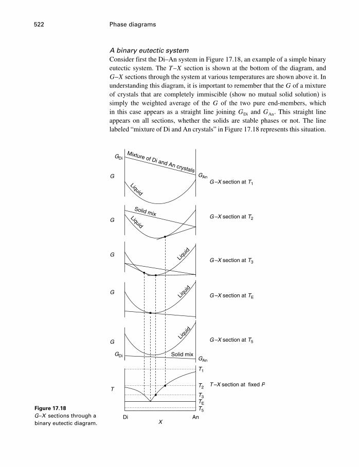
522 Phase diagrams
A binary eutectic systemConsider first the Di–An system in Figure 17.18, an example of a simple binaryeutectic system. The T–X section is shown at the bottom of the diagram, andG–X sections through the system at various temperatures are shown above it. Inunderstanding this diagram, it is important to remember that the G of a mixtureof crystals that are completely immiscible (show no mutual solid solution) issimply the weighted average of the G of the two pure end-members, whichin this case appears as a straight line joining GDi and GAn. This straight lineappears on all sections, whether the solids are stable phases or not. The linelabeled “mixture of Di and An crystals” in Figure 17.18 represents this situation.
Figure 17.18G–X sections through abinary eutectic diagram.
GDi
G
G
G
G
G
GAn
GAn
G –X section at T5
T –X section at fixed P
T1
T2
T3TET5
AnDiX
T
GDi Solid mix
G –X section at TE
G –X section at T3
G –X section at T2
G –X section at T1
Mixture of Di and An crystals
Liquid
Liquid
Liquid
Liquid
Liquid
Solid mix
17.3 Binary systems 523
When components do mutually dissolve to form a solution, Equation (10.4)still works for volumes if the solution is ideal, but even for ideal solutions, itdoes not work for G. The Gibbs energy of the solution must be less than theweighted average of the G of the two pure end-members for mutual solution totake place, and it is represented by the “festoon,” or convex-downward loop.Therefore, the liquid solution formed when liquid Di and liquid are mixedtogether is represented by such a loop. It is shown in all sections, even whenthe liquid is not the stable phase.
Understanding these G–X sections is helped by realizing that
• The line representing the G of the mixture of solid Di and solid An is shown in every
section regardless of whether diopside or anorthite is or is not stable. If they are not
stable, the line represents metastable Gibbs energies.• The line (festoon) representing the G of the complete liquid solution between Di and
An is shown in all sections regardless of whether the liquid is stable or not. If the
liquid is not stable, its curve represents metastable Gibbs energies.• The stable phase or phases in each section must have the lowest free energy available.
Starting with the G–X section at T1 at the top of the diagram, we see thatfor every bulk composition between Di and An, the liquid Gibbs energy iseverywhere lower than the Gibbs energy of a mixture of solid Di and solidAn. In other words, the stable phase across the diagram is liquid. On theT–X section, note that at T1, we are above the melting temperatures of bothcomponents, and in the field of liquid at all compositions.
As we cool from T1 to T2, the Gibbs energy of liquids and solids (whetherstable or metastable) increases, but that of liquids increases more, so that atT2, the G of liquid An has become greater than that of solid An, but the G ofliquid Di remains less than that of solid Di. At some temperature between T1and T2 we must have passed a point where Gliquid
An =GsolidAn , that is, the melting
temperature of An. At T2, the stable form of pure Di is liquid, but the stableform of pure An is solid. The lowest Gibbs energy available to the system aswe go from Di toward An is liquid, but just after passing the minimum onthe curve, the lowest Gibbs energy available is neither liquid nor a mixture ofcrystals, but a mixture of liquid and An crystals. In this mixture, the Gibbsenergy of component An in the crystals must be the same as the Gibbs energyof component An in the liquid.
Recall from Figure 7.4 that the tangent to a Gibbs energy curve of a solutionhas intercepts giving the chemical potential of each component in the solution.Therefore, a tangent to the liquid curve that has an intercept on the An axisat the Gibbs energy of solid An will indicate that liquid composition in which�
liquidAn = �solid
An . That tangent point is, of course, at the composition of theliquidus at that temperature, as shown by the dotted line joining the G–Xsection at T2 with the T–X section. As the temperature falls below T2, thattangent, rooted on the An axis at the free energy of solid An (Gsolid
An ), moves to
524 Phase diagrams
greater Di compositions, because the liquid loop is moving up with respect tothe Gsolid
An point.At T3, solid diopside is now the stable phase on the Di side of the diagram,
and the tangent situation described above holds for both components. Withfalling temperature, the two tangent points move toward each other, becomingone tangent at TE, the eutectic temperature. Note that at TE there must be onlyone tangent because �Di and �An must be the same in all three break phases.2
On further cooling, the tangent breaks away from the liquid curve andbecomes a straight line below the liquid curve, giving the Gibbs energy ofa mixture of diopside and anorthite crystals just as in the section at T1. Thedifference is that now it is completely below the liquid curve, and therefore amixture of crystals is the stable configuration of the system.
A melting loop systemThe story is rather similar for G–X sections through a melting loop diagramat various temperatures (Figure 17.19). However, instead of dealing with theintersection of a solution curve, or festoon, and a straight line, we have the inter-section of two solution curves – one for the liquid solution and one for thesolid solution. If this seems confusing, go back to §10.6 and recall why a Gibbsenergy curve for a solution must be convex downward. Then remember thatthis applies whether the solution is solid, liquid, or gaseous. Finally, rememberthat in these sections (Figure 17.19) we plot the positions of both solutioncurves in every section, regardless of whether the solution is the stable phaseor not. The point is to determine which parts of which curves give, or combineto give, the lowest Gibbs energy available to the system at each compositionacross the system.
At the top of the diagram, the section is drawn at the melting temperatureof anorthite crystals. Therefore, the liquid and solid curves join at the Anaxis, because Gsolid
An = GliquidAn . Going toward component Ab, the liquid curve
is everywhere below the solid curve, showing that liquid is everywhere thestable phase at this temperature. Similarly, the section at TmAb
shows thatGsolid
Ab =GliquidAb , and that at compositions toward component An, the solid curve
is below the liquid curve, showing that at this temperature, a solid solution ofAb and An is the stable phase. At intermediate temperatures, the two curvesintersect. The liquid curve is lower on one side, and the solid curve is loweron the other side. Intermediate compositions have the lowest possible Gibbsenergy only by being a mixture of solid and liquid, and because the chemicalpotentials of both Ab and An must be the same in both phases, the compositionsof the two solutions at equilibrium must be given by the only common tangentto the two curves at each temperature.
2 If you think about this statement, and look at Equations (7.26), you will see why we said(§17.3.4) that phases never remain absolutely pure when heated together, at least according toour model.
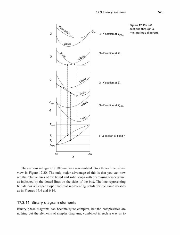
17.3 Binary systems 525
Solid solution
Liquid
G
G
G
GAb
G
Solid
Solid
Solid
Liquid
Liquid
Liquid
GAnG –X section at TmAn
G –X section at T2
G –X section at T1
G –X section at TmAb
T –X section at fixed P
TmAn
T1
T2
TmAb
Ab AnX
Figure 17.19 G–Xsections through amelting loop diagram.
The sections in Figure 17.19 have been reassembled into a three-dimensionalview in Figure 17.20. The only major advantage of this is that you can nowsee the relative rises of the liquid and solid loops with decreasing temperature,as indicated by the dotted lines on the sides of the box. The line representingliquids has a steeper slope than that representing solids for the same reasonsas in Figures 17.4 and 6.14.
17.3.11 Binary diagram elements
Binary phase diagrams can become quite complex, but the complexities arenothing but the elements of simpler diagrams, combined in such a way as to
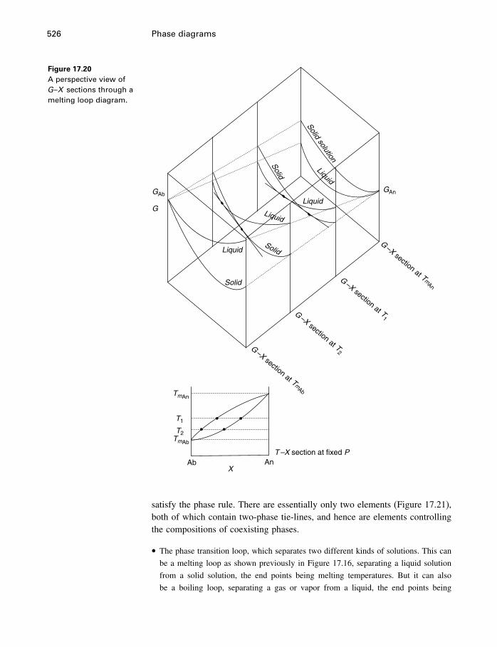
526 Phase diagrams
Figure 17.20A perspective view ofG–X sections through amelting loop diagram.
Solid solution
Solid
GAb
G
GAn
Liquid
Liquid
Liquid
Liquid
Solid
SolidG
–X section at TmAn
G–X
section at TmAb
G–X section at T
1G
–Xsection at T
2
TmAn
TmAb
T1
T2
AbX
AnT–X section at fixed P
satisfy the phase rule. There are essentially only two elements (Figure 17.21),both of which contain two-phase tie-lines, and hence are elements controllingthe compositions of coexisting phases.
• The phase transition loop, which separates two different kinds of solutions. This can
be a melting loop as shown previously in Figure 17.16, separating a liquid solution
from a solid solution, the end points being melting temperatures. But it can also
be a boiling loop, separating a gas or vapor from a liquid, the end points being
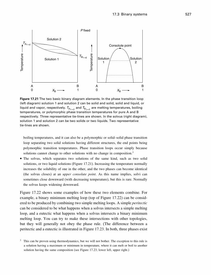
17.3 Binary systems 527
AXB0 1
B AXB0 1
B
Tem
pera
ture
Tem
pera
ture
TA1→2
TB1→2Solution 1
Solution 2
Solution1
Solution2
P fixed
Consolute point
Figure 17.21 The two basic binary diagram elements. In the phase transition loop(left diagram) solution 1 and solution 2 can be solid and solid, solid and liquid, orliquid and vapor, respectively. TA1→2
and TB1→2are melting temperatures, boiling
temperatures, or polymorphic phase transition temperatures for pure A and Brespectively. Three representative tie-lines are shown. In the solvus (right diagram),solution 1 and solution 2 can be two solids or two liquids. Two representativetie-lines are shown.
boiling temperatures, and it can also be a polymorphic or solid–solid phase transition
loop separating two solid solutions having different structures, the end points being
polymorphic transition temperatures. Phase transition loops occur simply because
solutions cannot change to other solutions with no change in composition.3
• The solvus, which separates two solutions of the same kind, such as two solid
solutions, or two liquid solutions (Figure 17.21). Increasing the temperature normally
increases the solubility of one in the other, and the two phases can become identical
(the solvus closes) at an upper consolute point. As this name implies, solvi can
sometimes close downward (with decreasing temperature), but this is rare. Normally
the solvus keeps widening downward.
Figure 17.22 shows some examples of how these two elements combine. Forexample, a binary minimum melting loop (top of Figure 17.22) can be consid-ered to be produced by combining two simple melting loops. A simple peritecticcan be considered to be what happens when a solvus intersects a simple meltingloop, and a eutectic what happens when a solvus intersects a binary minimummelting loop. You can try to make these intersections with other topologies,but they will generally not obey the phase rule. (The difference between aperitectic and a eutectic is illustrated in Figure 17.23. In both, three phases exist
3 This can be proven using thermodynamics, but we will not bother. The exception to this rule isa solution having a maximum or minimum in temperature, where it can melt or boil to anothersolution having the same composition (see Figure 17.23, lower left, upper right.)
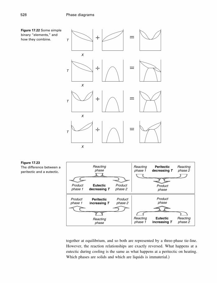
528 Phase diagrams
Figure 17.22 Some simplebinary “elements,” andhow they combine. T
X
X
X
X
T
T
T
Figure 17.23The difference between aperitectic and a eutectic.
Reactingphase
Reactingphase
Reactingphase 1
Reactingphase 2
Reactingphase 1
Reactingphase 2
Productphase 2
Productphase 1
Productphase 2
Productphase 1
Productphase
Productphase
Eutecticdecreasing T
Eutecticincreasing T
Peritecticdecreasing T
Peritecticincreasing T
together at equilibrium, and so both are represented by a three-phase tie-line.However, the reaction relationships are exactly reversed. What happens at aeutectic during cooling is the same as what happens at a peritectic on heating.Which phases are solids and which are liquids is immaterial.)
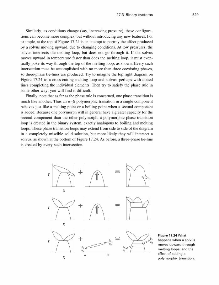
17.3 Binary systems 529
Similarly, as conditions change (say, increasing pressure), these configura-tions can become more complex, but without introducing any new features. Forexample, at the top of Figure 17.24 is an attempt to portray the effect producedby a solvus moving upward, due to changing conditions. At low pressures, thesolvus intersects the melting loop, but does not go through it. If the solvusmoves upward in temperature faster than does the melting loop, it must even-tually poke its way through the top of the melting loop, as shown. Every suchintersection must be accomplished with no more than three coexisting phases,so three-phase tie-lines are produced. Try to imagine the top right diagram onFigure 17.24 as a cross-cutting melting loop and solvus, perhaps with dottedlines completing the individual elements. Then try to satisfy the phase rule insome other way; you will find it difficult.
Finally, note that as far as the phase rule is concerned, one phase transition ismuch like another. Thus an –� polymorphic transition in a single componentbehaves just like a melting point or a boiling point when a second componentis added. Because one polymorph will in general have a greater capacity for thesecond component than the other polymorph, a polymorphic phase transitionloop is created in the binary system, exactly analogous to boiling and meltingloops. These phase transition loops may extend from side to side of the diagramin a completely miscible solid solution, but more likely they will intersect asolvus, as shown at the bottom of Figure 17.24. As before, a three-phase tie-lineis created by every such intersection.
T
T
X
X
X
T
A B
β1
β2β2
α2α2
α1
β1α1
Figure 17.24 Whathappens when a solvusmoves upward throughmelting loops, and theeffect of adding apolymorphic transition.
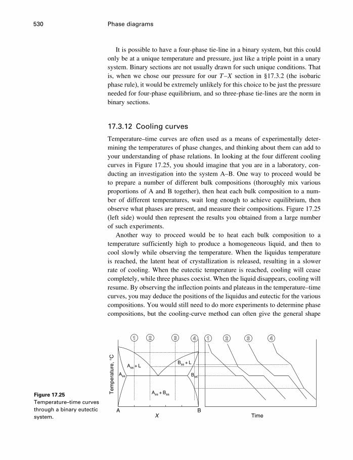
530 Phase diagrams
It is possible to have a four-phase tie-line in a binary system, but this couldonly be at a unique temperature and pressure, just like a triple point in a unarysystem. Binary sections are not usually drawn for such unique conditions. Thatis, when we chose our pressure for our T–X section in §17.3.2 (the isobaricphase rule), it would be extremely unlikely for this choice to be just the pressureneeded for four-phase equilibrium, and so three-phase tie-lines are the norm inbinary sections.
17.3.12 Cooling curves
Temperature–time curves are often used as a means of experimentally deter-mining the temperatures of phase changes, and thinking about them can add toyour understanding of phase relations. In looking at the four different coolingcurves in Figure 17.25, you should imagine that you are in a laboratory, con-ducting an investigation into the system A–B. One way to proceed would beto prepare a number of different bulk compositions (thoroughly mix variousproportions of A and B together), then heat each bulk composition to a num-ber of different temperatures, wait long enough to achieve equilibrium, thenobserve what phases are present, and measure their compositions. Figure 17.25(left side) would then represent the results you obtained from a large numberof such experiments.
Another way to proceed would be to heat each bulk composition to atemperature sufficiently high to produce a homogeneous liquid, and then tocool slowly while observing the temperature. When the liquidus temperatureis reached, the latent heat of crystallization is released, resulting in a slowerrate of cooling. When the eutectic temperature is reached, cooling will ceasecompletely, while three phases coexist. When the liquid disappears, cooling willresume. By observing the inflection points and plateaus in the temperature–timecurves, you may deduce the positions of the liquidus and eutectic for the variouscompositions. You would still need to do more experiments to determine phasecompositions, but the cooling-curve method can often give the general shape
Figure 17.25Temperature–time curvesthrough a binary eutecticsystem.
1 2 3 4 1 2 3 4
Tem
pera
ture
,°C
TimeXA B
Ass
Ass + LBss + L
Ass + Bss
Bss
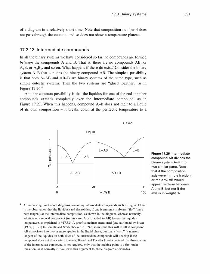
17.3 Binary systems 531
of a diagram in a relatively short time. Note that composition number 4 doesnot pass through the eutectic, and so does not show a temperature plateau.
17.3.13 Intermediate compounds
In all the binary systems we have considered so far, no compounds are formedbetween the compounds A and B. That is, there are no compounds AB, orA2B, or A2B3, and so on. What happens if these do exist? Consider the binarysystem A–B that contains the binary compound AB. The simplest possibilityis that both A–AB and AB–B are binary systems of the same type, such assimple eutectic systems. Then the two systems are “glued together,” as inFigure 17.26.4
Another common possibility is that the liquidus for one of the end-membercompounds extends completely over the intermediate compound, as inFigure 17.27. When this happens, compound A–B does not melt to a liquidof its own composition – it breaks down at the peritectic temperature to a
Tem
pera
ture
Liquid
L + A L + AB
A + AB AB + B
L + AB L + B
P fixed
A
0 100wt.% B
AB B
Figure 17.26 Intermediatecompound AB divides thebinary system A–B intotwo similar parts. Notethat if the compositionaxis were in mole fractionor mole %, AB wouldappear midway betweenA and B, but not if theaxis is in weight %.
4 An interesting point about diagrams containing intermediate compounds such as Figure 17.26is the observation that the liquidus (and the solidus, if one is present) is always “flat” (has azero tangent) at the intermediate composition, as shown in the diagram, whereas normally,addition of a second component (in this case, A or B added to AB) lowers the liquidustemperature, as explained in §17.3.5. A proof sometimes mentioned [and attributed by Pitzer(1995, p. 171) to Lorentz and Stortenbecker in 1892] shows that this will result if compoundAB dissociates into two or more species in the liquid phase, but that a “cusp” (a nonzerotangent of the liquidus on both sides of the intermediate compound) will develop if thecompound does not dissociate. However, Berndt and Diestler (1968) contend that dissociationof the intermediate compound is not required, only that the melting point is a first-ordertransition, as it normally is. We leave this argument to phase diagram aficionados.
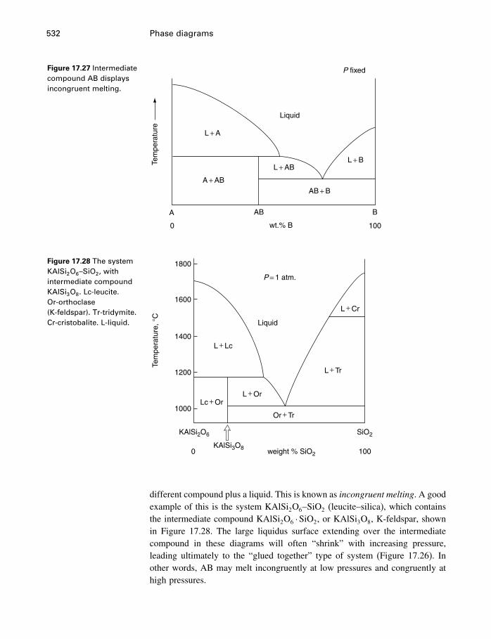
532 Phase diagrams
Figure 17.27 Intermediatecompound AB displaysincongruent melting.
Tem
pera
ture
Liquid
L + A
A + ABAB + B
L + ABL + B
P fixed
A
0 100wt.% B
AB B
Figure 17.28 The systemKAlSi2O6–SiO2, withintermediate compoundKAlSi3O8. Lc-leucite.Or-orthoclase(K-feldspar). Tr-tridymite.Cr-cristobalite. L-liquid.
1800
1600
1400
1200
1000
Tem
pera
ture
, °C
P = 1 atm.
KAlSi2O6
KAlSi3O8
SiO2
0 100weight % SiO2
Liquid
L + Lc
L + Cr
L + Tr
L + Or
Or + Tr
Lc + Or
different compound plus a liquid. This is known as incongruent melting. A goodexample of this is the system KAlSi2O6–SiO2 (leucite–silica), which containsthe intermediate compound KAlSi2O6 ·SiO2, or KAlSi3O8, K-feldspar, shownin Figure 17.28. The large liquidus surface extending over the intermediatecompound in these diagrams will often “shrink” with increasing pressure,leading ultimately to the “glued together” type of system (Figure 17.26). Inother words, AB may melt incongruently at low pressures and congruently athigh pressures.
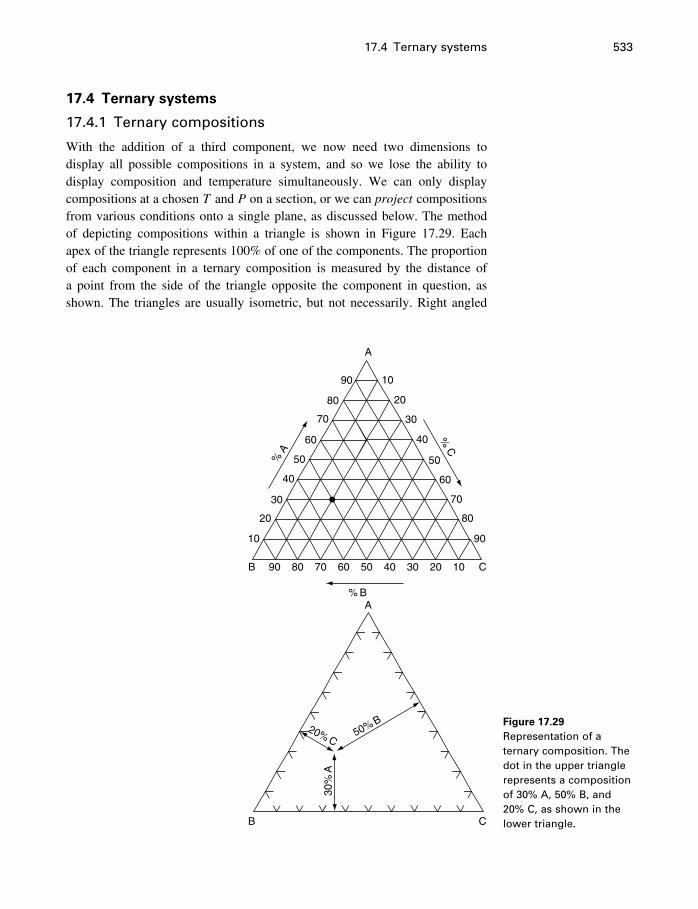
17.4 Ternary systems 533
17.4 Ternary systems
17.4.1 Ternary compositions
With the addition of a third component, we now need two dimensions todisplay all possible compositions in a system, and so we lose the ability todisplay composition and temperature simultaneously. We can only displaycompositions at a chosen T and P on a section, or we can project compositionsfrom various conditions onto a single plane, as discussed below. The methodof depicting compositions within a triangle is shown in Figure 17.29. Eachapex of the triangle represents 100% of one of the components. The proportionof each component in a ternary composition is measured by the distance ofa point from the side of the triangle opposite the component in question, asshown. The triangles are usually isometric, but not necessarily. Right angled
B
A
B
A
C
C
30%
A
50% B20% C
% B
% A
% C
10
20
20
20
30
30
30
40
40
40
5050
50
60
60
60
70
70
70
80
80
80
90
90
90
10
10
Figure 17.29Representation of aternary composition. Thedot in the upper trianglerepresents a compositionof 30% A, 50% B, and20% C, as shown in thelower triangle.
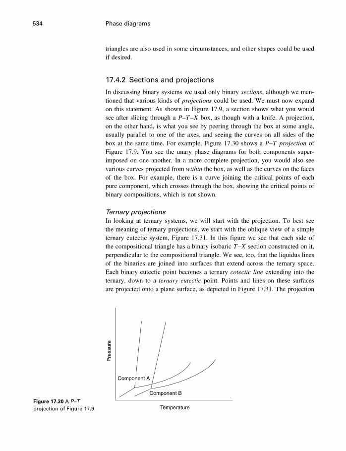
534 Phase diagrams
triangles are also used in some circumstances, and other shapes could be usedif desired.
17.4.2 Sections and projections
In discussing binary systems we used only binary sections, although we men-tioned that various kinds of projections could be used. We must now expandon this statement. As shown in Figure 17.9, a section shows what you wouldsee after slicing through a P–T–X box, as though with a knife. A projection,on the other hand, is what you see by peering through the box at some angle,usually parallel to one of the axes, and seeing the curves on all sides of thebox at the same time. For example, Figure 17.30 shows a P–T projection ofFigure 17.9. You see the unary phase diagrams for both components super-imposed on one another. In a more complete projection, you would also seevarious curves projected from within the box, as well as the curves on the facesof the box. For example, there is a curve joining the critical points of eachpure component, which crosses through the box, showing the critical points ofbinary compositions, which is not shown.
Ternary projectionsIn looking at ternary systems, we will start with the projection. To best seethe meaning of ternary projections, we start with the oblique view of a simpleternary eutectic system, Figure 17.31. In this figure we see that each side ofthe compositional triangle has a binary isobaric T–X section constructed on it,perpendicular to the compositional triangle. We see, too, that the liquidus linesof the binaries are joined into surfaces that extend across the ternary space.Each binary eutectic point becomes a ternary cotectic line extending into theternary, down to a ternary eutectic point. Points and lines on these surfacesare projected onto a plane surface, as depicted in Figure 17.31. The projection
Figure 17.30 A P –Tprojection of Figure 17.9. Temperature
Pre
ssur
e
Component A
Component B
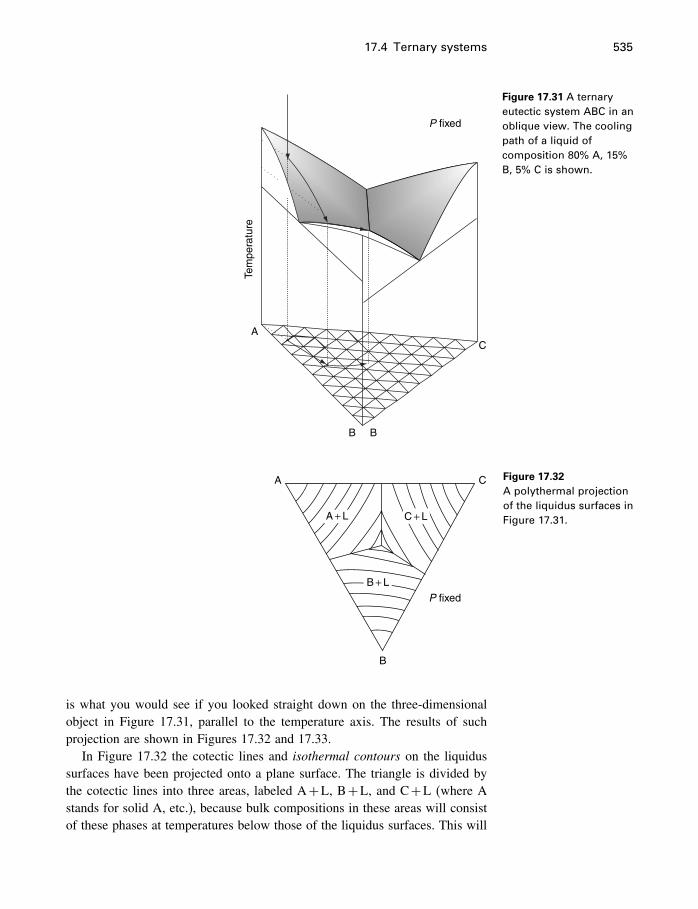
17.4 Ternary systems 535
Figure 17.31 A ternaryeutectic system ABC in anoblique view. The coolingpath of a liquid ofcomposition 80% A, 15%B, 5% C is shown.
AC
BB
P fixed
Tem
pera
ture
P fixed
A C
B
C + LA + L
B + L
Figure 17.32A polythermal projectionof the liquidus surfaces inFigure 17.31.
is what you would see if you looked straight down on the three-dimensionalobject in Figure 17.31, parallel to the temperature axis. The results of suchprojection are shown in Figures 17.32 and 17.33.
In Figure 17.32 the cotectic lines and isothermal contours on the liquidussurfaces have been projected onto a plane surface. The triangle is divided bythe cotectic lines into three areas, labeled A+L, B+L, and C+L (where Astands for solid A, etc.), because bulk compositions in these areas will consistof these phases at temperatures below those of the liquidus surfaces. This will
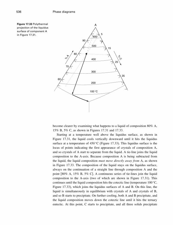
536 Phase diagrams
Figure 17.33 Polythermalprojection of the liquidussurface of component Ain Figure 17.31.
90
80
70
60
% A
% C
5
15
25
35
600
500
400
300
200
100 °C
A
become clearer by examining what happens to a liquid of composition 80% A,15% B, 5% C, as shown in Figures 17.31 and 17.33.
Starting at a temperature well above the liquidus surface, as shown inFigure 17.31, the liquid cools vertically downward until it hits the liquidussurface at a temperature of 450 �C (Figure 17.33). This liquidus surface is thelocus of points indicating the first appearance of crystals of composition A,and so crystals of A start to separate from the liquid. A tie-line joins the liquidcomposition to the A-axis. Because composition A is being subtracted fromthe liquid, the liquid composition must move directly away from A, as shownin Figure 17.33. The composition of the liquid stays on the liquidus surface,always on the continuation of a straight line through composition A and thepoint [80% A, 15% B, 5% C]. A continuous series of tie-lines join the liquidcomposition to the A-axis (two of which are shown in Figure 17.31). Thiscontinues until the liquid composition hits the cotectic line (temperature 100 �C,Figure 17.33), which joins the liquidus surfaces of A and B. On this line, theliquid is simultaneously in equilibrium with crystals of A and crystals of B,and so B starts to precipitate. On further cooling, both A and B precipitate, andthe liquid composition moves down the cotectic line until it hits the ternaryeutectic. At this point, C starts to precipitate, and all three solids precipitate
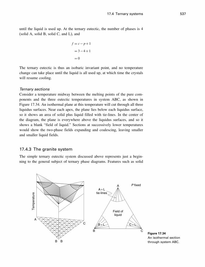
17.4 Ternary systems 537
until the liquid is used up. At the ternary eutectic, the number of phases is 4(solid A, solid B, solid C, and L), and
f = c−p+1
= 3−4+1
= 0
The ternary eutectic is thus an isobaric invariant point, and no temperaturechange can take place until the liquid is all used up, at which time the crystalswill resume cooling.
Ternary sectionsConsider a temperature midway between the melting points of the pure com-ponents and the three eutectic temperatures in system ABC, as shown inFigure 17.34. An isothermal plane at this temperature will cut through all threeliquidus surfaces. Near each apex, the plane lies below each liquidus surface,so it shows an area of solid plus liquid filled with tie-lines. In the center ofthe diagram, the plane is everywhere above the liquidus surfaces, and so itshows a blank “field of liquid.” Sections at successively lower temperatureswould show the two-phase fields expanding and coalescing, leaving smallerand smaller liquid fields.
17.4.3 The granite system
The simple ternary eutectic system discussed above represents just a begin-ning to the general subject of ternary phase diagrams. Features such as solid
Tem
pera
ture
AC
B B
A
CB
P fixedA + L
tie-lines
Field ofliquid
B + L C + L
Figure 17.34An isothermal sectionthrough system ABC.
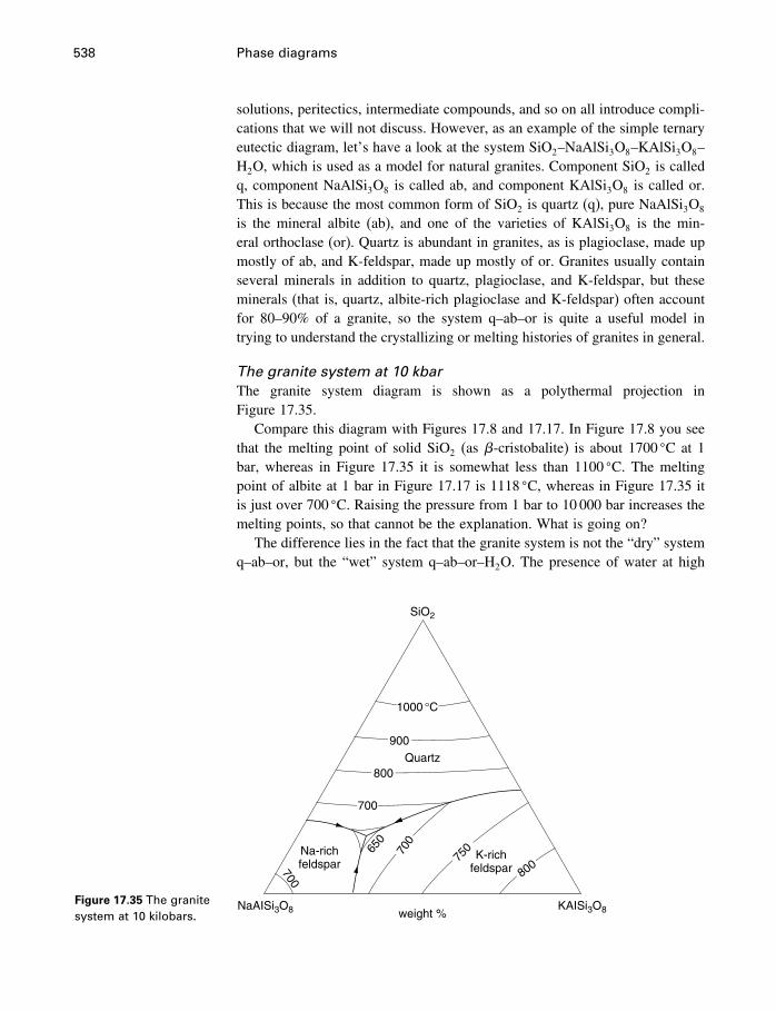
538 Phase diagrams
solutions, peritectics, intermediate compounds, and so on all introduce compli-cations that we will not discuss. However, as an example of the simple ternaryeutectic diagram, let’s have a look at the system SiO2–NaAlSi3O8–KAlSi3O8–H2O, which is used as a model for natural granites. Component SiO2 is calledq, component NaAlSi3O8 is called ab, and component KAlSi3O8 is called or.This is because the most common form of SiO2 is quartz (q), pure NaAlSi3O8
is the mineral albite (ab), and one of the varieties of KAlSi3O8 is the min-eral orthoclase (or). Quartz is abundant in granites, as is plagioclase, made upmostly of ab, and K-feldspar, made up mostly of or. Granites usually containseveral minerals in addition to quartz, plagioclase, and K-feldspar, but theseminerals (that is, quartz, albite-rich plagioclase and K-feldspar) often accountfor 80–90% of a granite, so the system q–ab–or is quite a useful model intrying to understand the crystallizing or melting histories of granites in general.
The granite system at 10 kbarThe granite system diagram is shown as a polythermal projection inFigure 17.35.
Compare this diagram with Figures 17.8 and 17.17. In Figure 17.8 you seethat the melting point of solid SiO2 (as �-cristobalite) is about 1700 �C at 1bar, whereas in Figure 17.35 it is somewhat less than 1100 �C. The meltingpoint of albite at 1 bar in Figure 17.17 is 1118 �C, whereas in Figure 17.35 itis just over 700 �C. Raising the pressure from 1 bar to 10 000 bar increases themelting points, so that cannot be the explanation. What is going on?
The difference lies in the fact that the granite system is not the “dry” systemq–ab–or, but the “wet” system q–ab–or–H2O. The presence of water at high
Figure 17.35 The granitesystem at 10 kilobars.
SiO2
1000 °C
900
800
700
700
700
800
75065
0
Quartz
Na-richfeldspar
K-richfeldspar
KAISi3O8NaAISi3O8 weight %
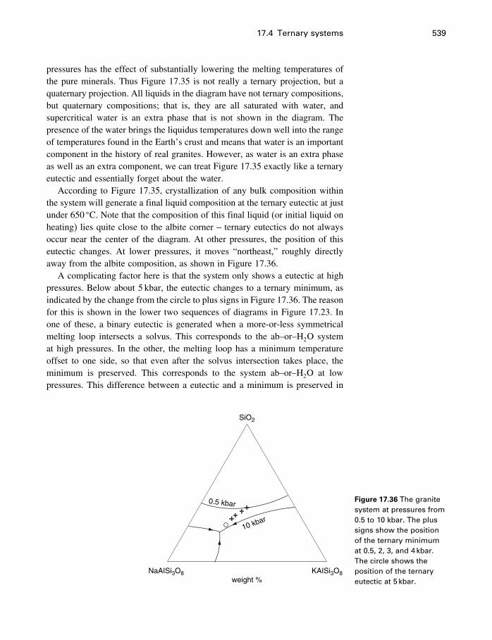
17.4 Ternary systems 539
pressures has the effect of substantially lowering the melting temperatures ofthe pure minerals. Thus Figure 17.35 is not really a ternary projection, but aquaternary projection. All liquids in the diagram have not ternary compositions,but quaternary compositions; that is, they are all saturated with water, andsupercritical water is an extra phase that is not shown in the diagram. Thepresence of the water brings the liquidus temperatures down well into the rangeof temperatures found in the Earth’s crust and means that water is an importantcomponent in the history of real granites. However, as water is an extra phaseas well as an extra component, we can treat Figure 17.35 exactly like a ternaryeutectic and essentially forget about the water.
According to Figure 17.35, crystallization of any bulk composition withinthe system will generate a final liquid composition at the ternary eutectic at justunder 650 �C. Note that the composition of this final liquid (or initial liquid onheating) lies quite close to the albite corner – ternary eutectics do not alwaysoccur near the center of the diagram. At other pressures, the position of thiseutectic changes. At lower pressures, it moves “northeast,” roughly directlyaway from the albite composition, as shown in Figure 17.36.
A complicating factor here is that the system only shows a eutectic at highpressures. Below about 5 kbar, the eutectic changes to a ternary minimum, asindicated by the change from the circle to plus signs in Figure 17.36. The reasonfor this is shown in the lower two sequences of diagrams in Figure 17.23. Inone of these, a binary eutectic is generated when a more-or-less symmetricalmelting loop intersects a solvus. This corresponds to the ab–or–H2O systemat high pressures. In the other, the melting loop has a minimum temperatureoffset to one side, so that even after the solvus intersection takes place, theminimum is preserved. This corresponds to the system ab–or–H2O at lowpressures. This difference between a eutectic and a minimum is preserved in
SiO2
KAISi3O8NaAISi3O8weight %
0.5 kbar
10 kbar
Figure 17.36 The granitesystem at pressures from0.5 to 10 kbar. The plussigns show the positionof the ternary minimumat 0.5, 2, 3, and 4 kbar.The circle shows theposition of the ternaryeutectic at 5 kbar.
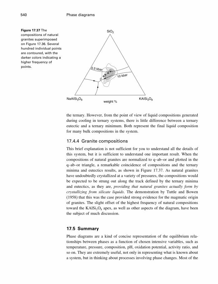
540 Phase diagrams
Figure 17.37 Thecompositions of naturalgranites superimposedon Figure 17.36. Severalhundred individual pointsare contoured, with thedarker colors indicating ahigher frequency ofpoints.
SiO2
KAISi3O8NaAISi3O8weight %
0.5 kbar
10 kbar
the ternary. However, from the point of view of liquid compositions generatedduring cooling in ternary systems, there is little difference between a ternaryeutectic and a ternary minimum. Both represent the final liquid compositionfor many bulk compositions in the system.
17.4.4 Granite compositions
This brief explanation is not sufficient for you to understand all the details ofthis system, but it is sufficient to understand one important result. When thecompositions of natural granites are normalized to q–ab–or and plotted in theq–ab–or triangle, a remarkable coincidence of compositions and the ternaryminima and eutectics results, as shown in Figure 17.37. As natural graniteshave undoubtedly crystallized at a variety of pressures, the compositions wouldbe expected to be strung out along the track defined by the ternary minimaand eutectics, as they are, providing that natural granites actually form bycrystallizing from silicate liquids. The demonstration by Tuttle and Bowen(1958) that this was the case provided strong evidence for the magmatic originof granites. The slight offset of the highest frequency of natural compositionstoward the KAlSi3O8 apex, as well as other aspects of the diagram, have beenthe subject of much discussion.
17.5 Summary
Phase diagrams are a kind of concise representation of the equilibrium rela-tionships between phases as a function of chosen intensive variables, such astemperature, pressure, composition, pH, oxidation potential, activity ratio, andso on. They are extremely useful, not only in representing what is known abouta system, but in thinking about processes involving phase changes. Most of the
17.5 Summary 541
diagrams in Chapters 12 and 14 are phase diagrams, although the term is mostoften used in relation to the P–T–X type of diagram discussed in this chapter.
Although in principle phase diagrams can be calculated from thermodynamicdata, in complex systems the relationships are generally determined experimen-tally. The diagrams must nevertheless obey rules established by equilibriumthermodynamics. Therefore an understanding of the material in all the previouschapters is a prerequisite to a real understanding of the simple points, lines,and surfaces found in phase diagrams.
The following extract is fromBridgman (1958: 423). It may help to dispel anynotion that determining phase relations is a simple and straightforward exercise.
Bridgman was a professor at Harvard University and in 1946 received theNobel Prize in physics for his research on materials at high pressures.
The conditions under which the different modifications of ice appear are
somewhat capricious, and often inconvenient manipulation is necessary to arrive
in the part of the phase diagram desired. The behavior is particularly striking in
the neighborhood of the V-VI-liquid triple point, say, between 0 �C and −10 �Cand between 5000 and 6000 bar. With the ordinary form of apparatus, water in
a steel piezometer with pressure transmitted to it by mercury, it is very difficult
to produce the modification V. For example, if liquid water at −10 �C is
compressed across the melting curve, the liquid will persist in the sub-cooled
condition for an indefinite time, without freezing to V, the stable form. But if
the compression is carried further, to the unstable prolongation of the liquid-VI
line, freezing to the form VI will take place almost at once on crossing the line,
in spite of the fact that VI is unstable with respect to V. Now in order to make
V appear, VI may be cooled 30� or 40�, when it will spontaneously change to
V, the stable form. If pressure is now released back to 5000, say, and
temperature is raised to the melting line of V, melting takes place at once and so
the coordinates of the melting line may be found. Suppose now after the melting
is completed the liquid water be kept in the neighborhood of the melting line
for several days, and then the pressure increased again across the melting line
at −10 �C; it will be found that the instant the melting line of V is crossed the
liquid freezes to V. This suggests that there has persisted in the liquid phase
some sort of structure, not detected by ordinary large-scale experiments,
favorable to the formation of V. It is now known, of course, from X-ray
analysis, that structures are possible in the liquid; this experiment suggests a
specificity in these structures that might well be the subject of further study.
The formation of the nucleus of V may be favored by the proper surface
conditions. Thus if there is any glass in contact with the liquid, either a
fragment of glass wool purposely introduced into the liquid, or by enclosing the
water in a glass instead of a steel bulb, freezing to V takes place at once
without the slightest hesitation immediately on carrying the virgin liquid across
the freezing line.
18Process modeling
18.1 Introduction
In this chapter we will have a brief look at how equilibrium thermodynamicsis used in dealing with processes, that is, reacting systems, rather than justsystems at equilibrium. Realistically, this should mean including the science ofchemical kinetics with our thermodynamics, and we should also include otherfactors, such as fluid flow, temperature and pressure gradients, and surfacereactions, to build increasingly realistic models of complex natural phenomenainvolving the movement and chemical reactions of fluids in soils and rocks inthe Earth’s crust.
That is all a bit too ambitious for this book. Computational models includingall these subjects are at the forefront of research in several areas. What we willattempt in this chapter is first, to outline the rudiments of chemical kinetics,and then show how equilibrium thermodynamics simulates chemically reactingsystems without using kinetics. The reason for discussing kinetics is that processmodeling in thermodynamics has some points in common with kinetics, becauseboth sciences consider the problem of chemical reactions proceeding fromstart to finish, and both use the progress variable. In simulating reactions inthermodynamics, however, we use the progress variable but not the real timevariable, with which it is closely connected in kinetics. The use of a real timevariable is what distinguishes kinetics from thermodynamics.
18.1.1 Quasi-static processes
In the following discussions, it will be useful to introduce the term quasi-static.This term has various meanings as used by various authors, but in this chapterit refers to an irreversible process carried out in a very large number of verysmall steps. The difference between a quasi-static and a reversible processis that the reversible process refers to a series of stable equilibrium states,while the quasi-static process is a series of metastable equilibrium states. Afterevery step of a reversible process, the system is at stable equilibrium with onlytwo constraints. After every step of a quasi-static process, the system is at ametastable equilibrium and has at least three constraints. This concept and theneed for it will become clear by considering some examples.
542
18.2 Kinetics 543
18.2 Kinetics
18.2.1 The myth of equilibrium
If you look around at the world we live in at the surface of planet Earth, itseems to be characterized by constant change; virtually nothing is permanent –even the solid rocks of the crust are weathering and being washed into thesea. And organic substances, including us, are among the most evanescent ofobjects – here today, gone tomorrow. Where are those states of equilibriumthat are so important in our thermodynamic model? It is in fact a tribute tothe creativity of the human mind that scientists were able to “see through” theconstant flux around them and create what is in essence a model of energyrelationships in a world that does not exist – the equilibrium world.
As we have seen in the last few chapters, this mathematical model of energyrelationships is tremendously useful in the real world, basically because eventhough the real world is in a constant state of flux or change, there are manysituations in which it approaches fairly closely a state of equilibrium, and evenin cases where it does not, it is changing towards some equilibrium state, andour equilibrium models are useful in many ways. But obviously we would liketo know more about the state of flux itself. How fast do the changes we see takeplace, and what controls this rate of change? We enter the world of chemicalkinetics.
18.2.2 The progress variable
Consider a generalized chemical reaction
aA+bB= cC+dD (18.1)
where A, B, C, and D are chemical formulas, and a, b, c, d are the stoichiometriccoefficients. We pointed out in §9.3 that when this reaction reaches equilibrium,
c�C+d�D = a�A+b�B
and
�r�= c�C+d�D−a�A−b�B (18.2)
= 0
Equation (18.1) can be generalized to∑i
�iMi = 0 (18.3)
where Mi are the chemical formulas and �i are the stoichiometric coefficients,with the stipulation that �i is positive for products and negative for reactants.Equation (18.2) can then be generalized to∑
i
�i�i = 0 (18.4)
544 Process modeling
Up to now, we have been most interested in reactions that reach equilibrium.Now let’s look at what happens before that point is reached, that is, whilethe reaction is taking place. Let’s say that the reaction proceeds from left toright as written. It doesn’t matter for the moment whether all the reactants andproducts are in the same phase (a homogeneous reaction) or in different phases(a heterogeneous reaction). During the reaction, A and B disappear and C andD appear, but the proportions of A:B:C:D that appear and disappear are fixedby the stoichiometric coefficients. If the reaction is
A+2B→ 3C+4D (18.5)
then for every mole of A that reacts (disappears), two moles of B must alsodisappear, while three moles of C and four moles of D must appear. This issimply a mass balance, independent of thermodynamics or kinetics, and can beexpressed as
dnA�A
= dnB�B
= dnC�C
= dnD�D
= dni�i
(18.6)
where, if all reactants and products are pure phases, the differentials dnA, dnB,and so on, can refer to a change in the amount of A, B, and so on, of anyconvenient magnitude, not necessarily an infinitesimal change. We can thenrepresent every term in (18.6) by a single variable d� so
dnA�A
= dnB�B
= dnC�C
= dnD�D
= d� (18.7)
from which it appears that
dnAd�
= �A�dnBd�
= �B� dnid�
= �i (18.8)
where our new variable � is called the reaction progress variable, and in thiscase represents an arbitrary number of moles. Equation (18.8) says that inreaction (18.5), dnA/d� =−1, dnB/d� =−2, dnC/d� = 3, and so on, whichsimply means that for every mole of A that disappears, two moles of B alsodisappear, three moles of C appear, and so on.
18.2.3 The reaction rate
Having defined reaction increments d�, we can now define the rate ofreaction as
d�
dt= 1�A
dnAdt
= 1�B
dnBdt
= = 1�i
dnidt
(18.9)
where dt is an increment of time, and d�/dt is the derivative of � with respectto t and is an expression of the amount of progress of the reaction as a functionof time, or simply the rate of reaction.
18.2 Kinetics 545
This expression (18.9) is written in terms of the absolute number of molesof A, B, and so on, (nA, nB,…), but by considering a fixed volume we couldchange these to concentration terms. Thus
d�
dt= 1�A
dCA
dt= 1�B
dCB
dt= = 1
�i
dCidt
(18.10)
where C is some unit of concentration such as mol cm−3.So evidently, the rate of reaction can be determined by measuring the
concentration of any of the reactants or products as a function of time. Withone important stipulation.
Elementary and overall reactionsIf you actually measure the rate of change of concentration of products andreactants in many ordinary chemical reactions, you find that the relationshipin (18.10) is often not obeyed. This is because the reaction does not actuallyproceed as written, at the molecular level. For example, reaction (18.5), takenliterally, indicates that a molecule of A reacts with two molecules of B, andat that instant, three molecules of C and four molecules of D are formed. Butthis might not be what happens at all, and in view of the improbability ofthree molecules (A+2B) meeting at a single point, it probably is not in thiscase. The reaction as written may well represent the overall result of a seriesof elementary reactions. Thus A and B may in fact react to form a numberof intermediate species such as X and Y, which then react with each otheror with A or B to form C and D. In thermodynamics, the existence of suchintermediate species is not important to the study of the overall reaction, as longas equilibrium is attained, but in kinetics, they contribute to the overall rate ofreaction and may actually be rate-controlling, even though their concentrationsmay be small.
Of course, it is also possible that intermediate species do form, but theyachieve a steady-state concentration, that is, they break up just as rapidly asthey form. In this case, Equation (18.10) would be obeyed, even though it didnot represent what actually happens at the molecular level.
From now on in this section, we will use = in overall reactions, and → inelementary reactions (those that actually proceed as written).
18.2.4 Rate laws
A rate law is a statement about how the rate of a reaction depends on the con-centrations of the participating species. If one thinks about chemical reactionsas something that happens at the molecular level when molecules collide withone another, it makes sense that the number of collisions, and hence the rate ofreaction, should depend on how many molecules of each type there are; that is,
546 Process modeling
their concentrations.1 In most cases, a simple power function of concentrationsis found to apply. For reaction (18.1) it is
rate of reaction= d�
dt= k ·CnAA CnBB CnCC CnDD (18.11)
The constant of proportionality, k, is called the rate constant. The exponentsnA nD are often integers, but can be fractional or decimal numbers, especiallyin heterogeneous reactions where adsorption and other surface-related effectscan influence reaction rates. They define the order of the reaction. If nA is 2,the reaction is said to be second order in A. The sum of the exponents givesthe overall order of the reaction.
The rate laws for chemical reactions are expressions that best fit experimentaldata, and the order of reaction is the sum of the experimentally determinedexponents.
Rate laws for elementary reactionsRate laws are determined by analyzing one or more reactant or product speciesas a function of time as a reaction proceeds, and then inspecting the results tosee what theoretical form best fits the data.
First orderRate laws for elementary reactions are for the most part what one would expect.For example, a simple molecular (or nuclear) decomposition,
A→ products
proceeds at a rate that depends only on the concentration of A; the more A,the more decomposition per unit time. The rate law is
d�
dt=−dCA
dt= k ·CA (18.12)
and the reaction is first order. The decay of radioactive elements is an exampleof such reactions.
If we simplify CA to C and let C = C� at time t = 0, integration of (18.12)gives ∫ C
C�dC
C=−k
∫ t
0dt (18.13)
lnC�
C= kt (18.14)
lnC = lnC� −kt (18.15)
C = C�e−kt (18.16)
1 In thermodynamics, we must use “corrected” concentrations, or activities. In kinetics it is theactual concentrations that are important.
18.2 Kinetics 547
These equations suggest various ways of plotting data to see if they fit a firstorder rate law. For example, a plot of ln�C�/C� versus t will give a straightline with a slope equal to the rate constant for concentration data from a firstorder reaction.
Second order
The most common type of elementary reaction results from bimolecularcollisions:
A+B→ products (18.17)
Here we expect the frequency of reaction to be proportional to the concentra-tions of the reactants and the concentration of products to have no effect, andso the rate law is
d�
dt=−dCA
dt=−dCB
dt= k ·C1
AC1B (18.18)
and the reaction is second order.If the initial concentrations of A and B are C�
A and C�B, the stoichiometry of
(18.17) requires that
C�A−CA = C�
B−CB
Solving this for CB and substituting this result in (18.18) gives
−dCA
dt= k ·CA�CA−C�
A+C�B� (18.19)
Integration of (18.19) then gives
ln(C�
ACB
C�BCA
)= �C�
B−C�A�kt (18.20)
Therefore, a plot of (1
C�B−C�
A
)ln(C�
ACB
C�BCA
)
versus time t will result in a straight line with a slope equal to the rate constantfor concentrations taken from a second order reaction. Similar equations canbe derived for reactions with different stoichiometric coefficients.
There are a number of other rate laws, but this will suffice to give anidea of the procedures involved. However, it should be emphasized that mostchemical reactions are “overall” reactions, and that their understanding in terms
548 Process modeling
of their fundamental elementary reactions is a goal not often and not easilyachieved.
18.2.5 Temperature dependence of rate constants
In §9.6 we saw that the temperature dependence of the equilibrium constant Kcould be expressed as
d lnKd�1/T�
=−�rH�
R
or, alternatively
d lnKdT
= �rH�
RT 2
In 1889, Arrhenius proposed a similar equation for the temperature effect onrate constants,
d ln kd�1/T�
=−Ea
R(18.21)
or
d ln kdT
= Ea
RT 2(18.22)
where Ea is called the Arrhenius activation energy, or just the activation energy,and turns out to be closely related to the “energy barrier” between productsand reactants in chemical reactions. The general form of this equation has beenshown to be derivable from statistical mechanics.
Experimental data for a great many reactions over a large range of temper-atures shows that the Arrhenius equation is usually closely obeyed, showingthat Ea is either a constant or a weak function of temperature, and so we canintegrate the equation to give
ln k= lnA− Ea
RT(18.23)
or
k= Ae−Ea/RT (18.24)
where A, which enters (18.23) as a constant of integration, is called thepre-exponential factor.
The activation energy of an overall reaction is made up of the individualcontributions of the elementary reactions making up the overall reaction. Themagnitude of the activation energy can vary from virtually zero to hundredsof kJ per mole and, besides controlling the temperature dependence of the rateconstant, provides clues as to the nature of the reaction mechanisms, becausethe energies involved in many types of diffusion, electron exchange, and bond-breaking processes are known.
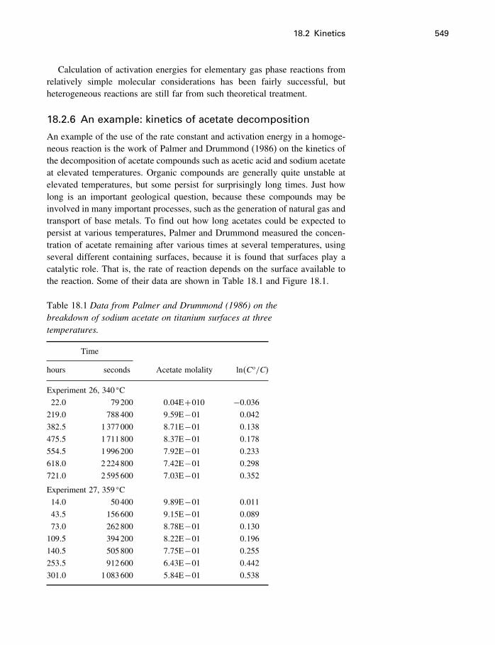
18.2 Kinetics 549
Calculation of activation energies for elementary gas phase reactions fromrelatively simple molecular considerations has been fairly successful, butheterogeneous reactions are still far from such theoretical treatment.
18.2.6 An example: kinetics of acetate decomposition
An example of the use of the rate constant and activation energy in a homoge-neous reaction is the work of Palmer and Drummond (1986) on the kinetics ofthe decomposition of acetate compounds such as acetic acid and sodium acetateat elevated temperatures. Organic compounds are generally quite unstable atelevated temperatures, but some persist for surprisingly long times. Just howlong is an important geological question, because these compounds may beinvolved in many important processes, such as the generation of natural gas andtransport of base metals. To find out how long acetates could be expected topersist at various temperatures, Palmer and Drummond measured the concen-tration of acetate remaining after various times at several temperatures, usingseveral different containing surfaces, because it is found that surfaces play acatalytic role. That is, the rate of reaction depends on the surface available tothe reaction. Some of their data are shown in Table 18.1 and Figure 18.1.
Table 18.1 Data from Palmer and Drummond (1986) on thebreakdown of sodium acetate on titanium surfaces at threetemperatures.
Time
hours seconds Acetate molality ln�Co/C�
Experiment 26, 340 �C22�0 79200 0�04E+010 −0�036
219�0 788400 9�59E−01 0�042
382�5 1377000 8�71E−01 0�138
475�5 1711800 8�37E−01 0�178
554�5 1996200 7�92E−01 0�233
618�0 2224800 7�42E−01 0�298
721�0 2595600 7�03E−01 0�352
Experiment 27, 359 �C14�0 50400 9�89E−01 0�011
43�5 156600 9�15E−01 0�089
73�0 262800 8�78E−01 0�130
109�5 394200 8�22E−01 0�196
140�5 505800 7�75E−01 0�255
253�5 912600 6�43E−01 0�442
301�0 1083600 5�84E−01 0�538
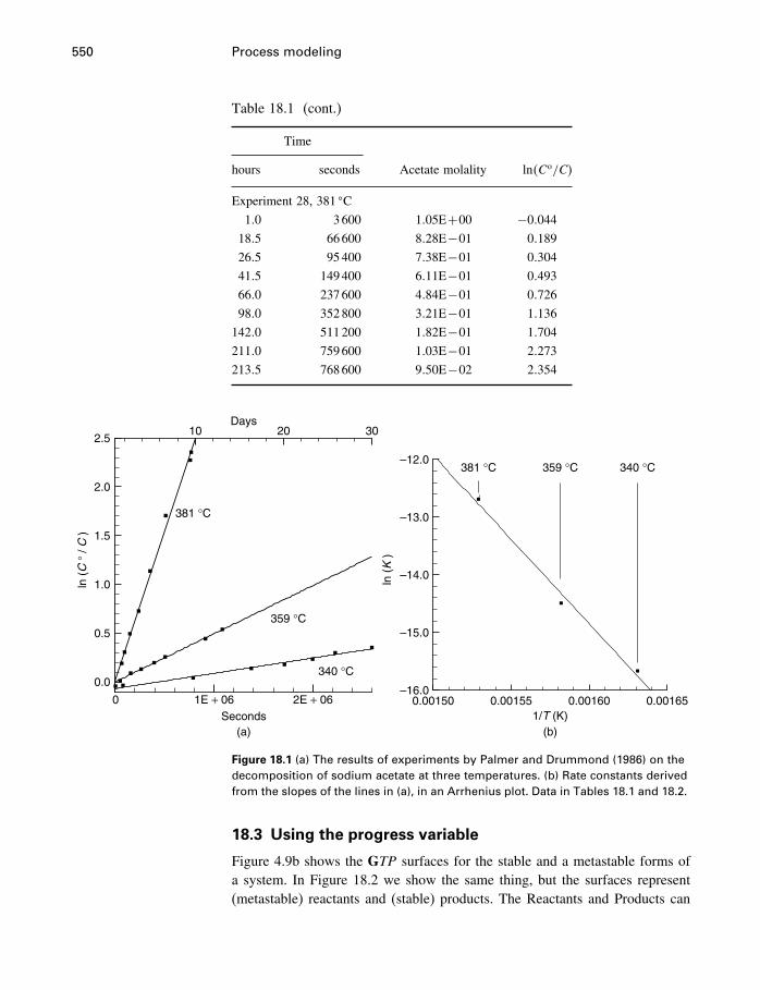
550 Process modeling
Table 18.1 (cont.)
Time
hours seconds Acetate molality ln�Co/C�
Experiment 28, 381 �C1�0 3600 1�05E+00 −0�044
18�5 66600 8�28E−01 0�189
26�5 95400 7�38E−01 0�304
41�5 149400 6�11E−01 0�493
66�0 237600 4�84E−01 0�726
98�0 352800 3�21E−01 1�136
142�0 511200 1�82E−01 1�704
211�0 759600 1�03E−01 2�273
213�5 768600 9�50E−02 2�354
Seconds
Days
ln (
C° /
C )
0 1E + 06 2E + 06
10 20 30
0.0
0.5
1.0
1.5
2.0
2.5
340 °C
359 °C
381 °C
(a)1/T (K)
ln (
K)
0.00150 0.00155 0.00160 0.00165–16.0
–15.0
–14.0
–13.0
–12.0340 °C359 °C381 °C
(b)
Figure 18.1 (a) The results of experiments by Palmer and Drummond (1986) on thedecomposition of sodium acetate at three temperatures. (b) Rate constants derivedfrom the slopes of the lines in (a), in an Arrhenius plot. Data in Tables 18.1 and 18.2.
18.3 Using the progress variable
Figure 4.9b shows the GTP surfaces for the stable and a metastable forms ofa system. In Figure 18.2 we show the same thing, but the surfaces represent(metastable) reactants and (stable) products. The Reactants and Products can
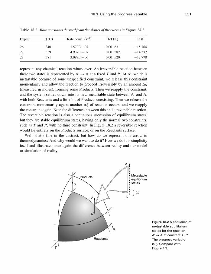
18.3 Using the progress variable 551
Table 18.2 Rate constants derived from the slopes of the curves in Figure 18.1.
Expmt T( �C) Rate const. (s−1) 1/T (K) lnK
26 340 1.570E− 07 0.001 631 −15.764
27 359 4.937E− 07 0.001 582 −14.332
28 381 3.087E− 06 0.001 529 −12.778
represent any chemical reaction whatsoever. An irreversible reaction betweenthese two states is represented by A′ → A at a fixed T and P. At A′, which ismetastable because of some unspecified constraint, we release this constraintmomentarily and allow the reaction to proceed irreversibly by an amount ��(measured in moles), forming some Products. Then we reapply the constraint,and the system settles down into its new metastable state between A′ and A,with both Reactants and a little bit of Products coexisting. Then we release theconstraint momentarily again, another �� of reaction occurs, and we reapplythe constraint again. Note the difference between this and a reversible reaction.The reversible reaction is also a continuous succession of equilibrium states,but they are stable equilibrium states, having only the normal two constraints,such as T and P, with no third constraint. In Figure 18.2 a reversible reactionwould lie entirely on the Products surface, or on the Reactants surface.
Well, that’s fine in the abstract, but how do we represent this arrow inthermodynamics? And why would we want to do it? How we do it is simplicityitself and illustrates once again the difference between reality and our modelor simulation of reality.
Products Metastableequilibriumstates
Reactants
P
T
A′
A′A
G
A
∆ξ
Figure 18.2 A sequence ofmetastable equilibriumstates for the reactionA′ → A at constant T , P .The progress variableis �. Compare withFigure 4.9.
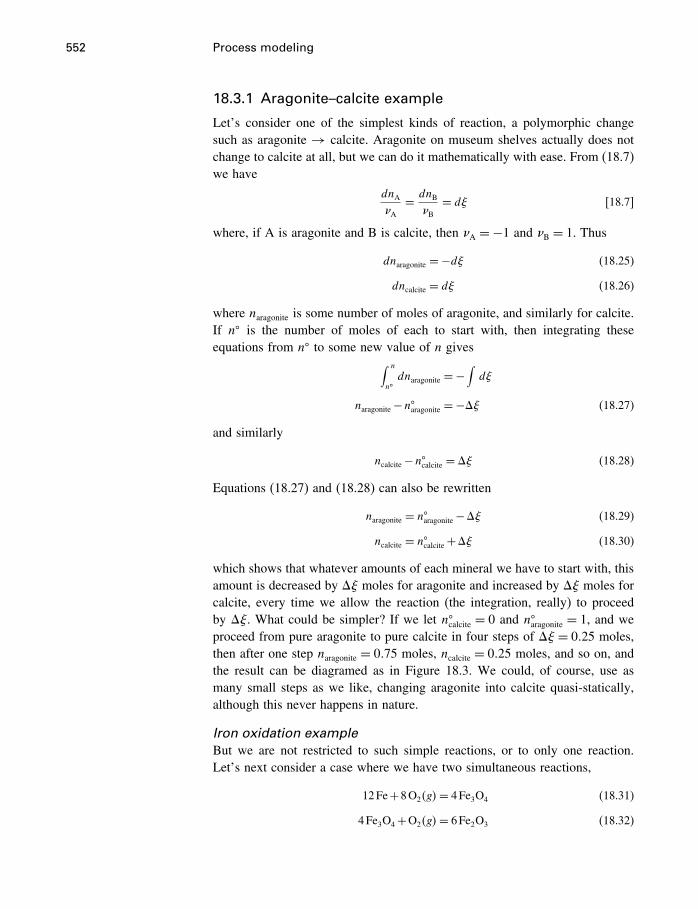
552 Process modeling
18.3.1 Aragonite–calcite example
Let’s consider one of the simplest kinds of reaction, a polymorphic changesuch as aragonite → calcite. Aragonite on museum shelves actually does notchange to calcite at all, but we can do it mathematically with ease. From (18.7)we have
dnA�A
= dnB�B
= d� [18.7]
where, if A is aragonite and B is calcite, then �A =−1 and �B = 1. Thus
dnaragonite =−d� (18.25)
dncalcite = d� (18.26)
where naragonite is some number of moles of aragonite, and similarly for calcite.If n� is the number of moles of each to start with, then integrating theseequations from n� to some new value of n gives∫ n
n�dnaragonite =−
∫d�
naragonite−n�aragonite =−�� (18.27)
and similarly
ncalcite−n�calcite = �� (18.28)
Equations (18.27) and (18.28) can also be rewritten
naragonite = n�aragonite−�� (18.29)
ncalcite = n�calcite+�� (18.30)
which shows that whatever amounts of each mineral we have to start with, thisamount is decreased by �� moles for aragonite and increased by �� moles forcalcite, every time we allow the reaction (the integration, really) to proceedby ��. What could be simpler? If we let n�calcite = 0 and n�aragonite = 1, and weproceed from pure aragonite to pure calcite in four steps of �� = 0�25 moles,then after one step naragonite = 0�75 moles, ncalcite = 0�25 moles, and so on, andthe result can be diagramed as in Figure 18.3. We could, of course, use asmany small steps as we like, changing aragonite into calcite quasi-statically,although this never happens in nature.
Iron oxidation exampleBut we are not restricted to such simple reactions, or to only one reaction.Let’s next consider a case where we have two simultaneous reactions,
12Fe+8O2�g�= 4Fe3O4 (18.31)
4Fe3O4+O2�g�= 6Fe2O3 (18.32)
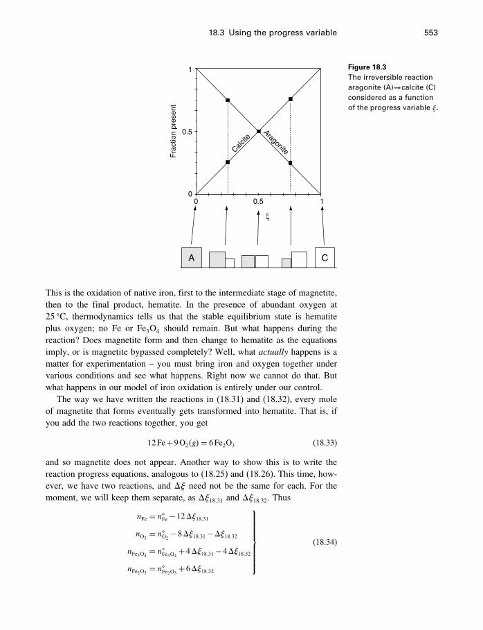
18.3 Using the progress variable 553
0.50 1
0.5
1
0
Fra
ctio
n pr
esen
t
Calcite
Aragonite
A C
ξ
Figure 18.3The irreversible reactionaragonite (A)→calcite (C)considered as a functionof the progress variable �.
This is the oxidation of native iron, first to the intermediate stage of magnetite,then to the final product, hematite. In the presence of abundant oxygen at25 �C, thermodynamics tells us that the stable equilibrium state is hematiteplus oxygen; no Fe or Fe3O4 should remain. But what happens during thereaction? Does magnetite form and then change to hematite as the equationsimply, or is magnetite bypassed completely? Well, what actually happens is amatter for experimentation – you must bring iron and oxygen together undervarious conditions and see what happens. Right now we cannot do that. Butwhat happens in our model of iron oxidation is entirely under our control.
The way we have written the reactions in (18.31) and (18.32), every moleof magnetite that forms eventually gets transformed into hematite. That is, ifyou add the two reactions together, you get
12Fe+9O2�g�= 6Fe2O3 (18.33)
and so magnetite does not appear. Another way to show this is to write thereaction progress equations, analogous to (18.25) and (18.26). This time, how-ever, we have two reactions, and �� need not be the same for each. For themoment, we will keep them separate, as ��18�31 and ��18�32. Thus
nFe = n�Fe−12��18�31
nO2= n�O2
−8��18�31−��18�32nFe3O4
= n�Fe3O4+4��18�31−4��18�32
nFe2O3= n�Fe2O3
+6��18�32
⎫⎪⎪⎪⎪⎪⎪⎪⎬⎪⎪⎪⎪⎪⎪⎪⎭(18.34)
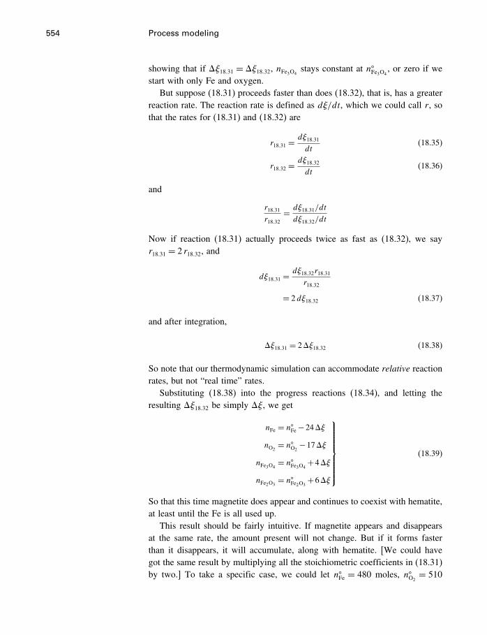
554 Process modeling
showing that if ��18�31 = ��18�32, nFe3O4stays constant at n�Fe3O4
, or zero if westart with only Fe and oxygen.
But suppose (18.31) proceeds faster than does (18.32), that is, has a greaterreaction rate. The reaction rate is defined as d�/dt, which we could call r , sothat the rates for (18.31) and (18.32) are
r18�31 =d�18�31dt
(18.35)
r18�32 =d�18�32dt
(18.36)
and
r18�31r18�32
= d�18�31/dt
d�18�32/dt
Now if reaction (18.31) actually proceeds twice as fast as (18.32), we sayr18�31 = 2 r18�32, and
d�18�31 =d�18�32r18�31r18�32
= 2d�18�32 (18.37)
and after integration,
��18�31 = 2��18�32 (18.38)
So note that our thermodynamic simulation can accommodate relative reactionrates, but not “real time” rates.
Substituting (18.38) into the progress reactions (18.34), and letting theresulting ��18�32 be simply ��, we get
nFe = n�Fe−24��
nO2= n�O2
−17��
nFe3O4= n�Fe3O4
+4��
nFe2O3= n�Fe2O3
+6��
⎫⎪⎪⎪⎪⎪⎪⎪⎬⎪⎪⎪⎪⎪⎪⎪⎭(18.39)
So that this time magnetite does appear and continues to coexist with hematite,at least until the Fe is all used up.
This result should be fairly intuitive. If magnetite appears and disappearsat the same rate, the amount present will not change. But if it forms fasterthan it disappears, it will accumulate, along with hematite. [We could havegot the same result by multiplying all the stoichiometric coefficients in (18.31)by two.] To take a specific case, we could let n�Fe = 480 moles, n�O2
= 510
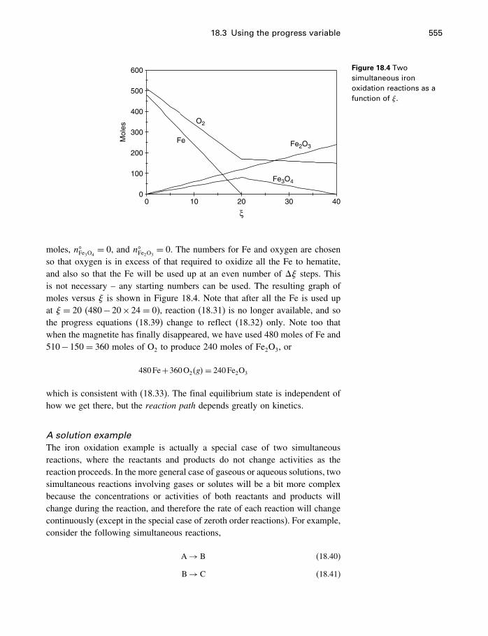
18.3 Using the progress variable 555
600
500
O2
FeMol
es
Fe2O3
Fe3O4
400
300
200
100
00 10 20 30 40
ξ
Figure 18.4 Twosimultaneous ironoxidation reactions as afunction of �.
moles, n�Fe3O4= 0, and n�Fe2O3
= 0. The numbers for Fe and oxygen are chosenso that oxygen is in excess of that required to oxidize all the Fe to hematite,and also so that the Fe will be used up at an even number of �� steps. Thisis not necessary – any starting numbers can be used. The resulting graph ofmoles versus � is shown in Figure 18.4. Note that after all the Fe is used upat � = 20 (480−20×24 = 0), reaction (18.31) is no longer available, and sothe progress equations (18.39) change to reflect (18.32) only. Note too thatwhen the magnetite has finally disappeared, we have used 480 moles of Fe and510−150= 360 moles of O2 to produce 240 moles of Fe2O3, or
480Fe+360O2�g�= 240Fe2O3
which is consistent with (18.33). The final equilibrium state is independent ofhow we get there, but the reaction path depends greatly on kinetics.
A solution exampleThe iron oxidation example is actually a special case of two simultaneousreactions, where the reactants and products do not change activities as thereaction proceeds. In the more general case of gaseous or aqueous solutions, twosimultaneous reactions involving gases or solutes will be a bit more complexbecause the concentrations or activities of both reactants and products willchange during the reaction, and therefore the rate of each reaction will changecontinuously (except in the special case of zeroth order reactions). For example,consider the following simultaneous reactions,
A→ B (18.40)
B→ C (18.41)
556 Process modeling
where A, B, and C can be gaseous compounds or aqueous solutes, and wherethe rate constants are k18�40 for A→ B, and k18�41 for B→ C. The rate equationsare [cf. (18.12)]
−dCA
dt= k18�40CA (18.42)
dCB
dt= k18�40CA−k18�41CB (18.43)
dCC
dt= k18�41CB (18.44)
If the initial concentrations are C�A, C
�B = 0, and C�
C = 0, (18.42) gives
CA = C�Ae
−k18�40t
Equation (18.43) then becomes
dCB
dt= k18�40C�
Ae−k18�40t−k18�41CB (18.45)
With a little ingenuity, this is integrated to give
CB = k18�40C�A
�k18�41−k18�40�(e−k18�40t− e−k18�41t) (18.46)
Then CC is obtained from the mass balance,
CC = C�A−CA−CB (18.47)
The result, for k18�40 = 1� k18�41 = 0�5, is shown in Figure 18.5. Note the gen-eral similarity to Figure 18.4, in the sense that the intermediate compound(B, Fe3O4) accumulates, then disappears as equilibrium is approached. Theamount of intermediates formed is controlled entirely by the kinetics of thereactions.
Figure 18.5Two simultaneous gasreactions as a function oftime, t.
10
8
6
4
2
00
A
B
C
Time, t
2 4 6 8 10
Con
cent
ratio
n
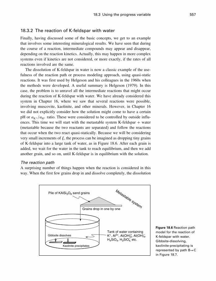
18.3 Using the progress variable 557
18.3.2 The reaction of K-feldspar with water
Finally, having discussed some of the basic concepts, we get to an examplethat involves some interesting mineralogical results. We have seen that duringthe course of a reaction, intermediate compounds may appear and disappear,depending on the reaction kinetics. Actually, this may happen in more complexsystems even if kinetics are not considered, or more exactly, if the rates of allreactions involved are the same.
The dissolution of K-feldspar in water is now a classic example of the use-fulness of the reaction path or process modeling approach, using quasi-staticreactions. It was first used by Helgeson and his colleagues in the 1960s whenthe methods were developed. A useful summary is Helgeson (1979). In thiscase, the problem is to unravel all the intermediate reactions that might occurduring the reaction of K-feldspar with water. We have already considered thissystem in Chapter 16, where we saw that several reactions were possible,involving muscovite, kaolinite, and other minerals. However, in Chapter 16we did not explicitly consider how the solution might come to have a certainpH or aK+/aH+ ratio. These were considered to be controlled by outside influ-ences. This time we will start with the metastable system K-feldspar + water(metastable because the two reactants are separated) and follow the reactionsthat occur when the two react quasi-statically. Because we will be consideringvery small increments of �, the process can be imagined as dropping tiny grainsof K-feldspar into a large tank of water, as in Figure 18.6. After each grain isadded, we wait for the water in the tank to reach equilibrium, and then we addanother grain, and so on, until K-feldspar is in equilibrium with the solution.
The reaction pathA surprising number of things happen when the reaction is considered in thisway. When the first few grains drop in and dissolve completely, the dissolution
Pile of KAlSi3O8 sand grains
Grains drop in one by one
Metastable system
Gibbsite dissolves
Kaolinite precipitates
Tank of water containingK+, Al3+, Al(OH)2, Al(OH)4,H4SiO4, H3SiO4, etc.
–
–
+
Figure 18.6 Reaction pathmodel for the reaction ofK-feldspar with water.Gibbsite-dissolving,kaolinite-precipitating isrepresented by path B→Cin Figure 18.7.
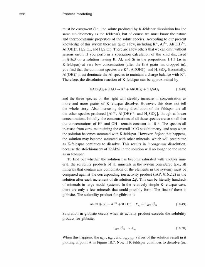
558 Process modeling
must be congruent (i.e., the solute produced by K-feldspar dissolution has thesame stoichiometry as the feldspar), but of course we must know the natureand thermodynamic properties of the solute species. According to our presentknowledge of this system there are quite a few, including K+, Al3+, Al�OH�2+,Al�OH�−4 , H4SiO4, and H3SiO
−4 . There are a few others that we can omit without
serious error. If you perform a speciation calculation of the kind discussedin §16.3 on a solution having K, Al, and Si in the proportions 1:1:3 (as inK-feldspar) at very low concentration (after the first grain has dropped in),you find that the dominant species are K+, Al�OH�−4 , and H4SiO4. Essentially,Al�OH�−4 must dominate the Al species to maintain a charge balance with K+.Therefore, the dissolution reaction of K-feldspar can be approximated by
KAlSi3O8+8H2O→ K++Al�OH�−4 +3H4SiO4 (18.48)
and the three species on the right will steadily increase in concentration asmore and more grains of K-feldspar dissolve. However, this does not tellthe whole story. Also increasing during dissolution of the feldspar are allthe other species produced [Al3+, Al�OH�2+, and H3SiO
−4 ], though at lower
concentrations. Initially, the concentrations of all these species are so small thatthe concentrations of H+ and OH− remain constant at 10−7. The species allincrease from zero, maintaining the overall 1:1:3 stoichiometry, and stop whenthe solution becomes saturated with K-feldspar. However, before that happens,the solution may become saturated with other minerals, which will precipitateas K-feldspar continues to dissolve. This results in incongruent dissolution,because the stoichiometry of K:Al:Si in the solution will no longer be the sameas in feldspar.
To find out whether the solution has become saturated with another min-eral, the solubility products of all minerals in the system considered (i.e., allminerals that contain any combination of the elements in the system) must becompared against the corresponding ion activity product (IAP, §16.2.2) in thesolution after each increment of dissolution ��. This can be literally hundredsof minerals in large model systems. In the relatively simple K-feldspar case,there are only a few minerals that could possibly form. The first of these isgibbsite. The solubility product for gibbsite is
Al�OH�3�s�= Al3++3OH−� Ksp = aAl3+a3OH− (18.49)
Saturation in gibbsite occurs when its activity product exceeds the solubilityproduct for gibbsite:
aAl3+a3OH− >Ksp (18.50)
When this happens, the aK+ , aH+ , and aSiO2�aq�values of the solution result in it
plotting at point A in Figure 18.7. Now if K-feldspar continues to dissolve (or,
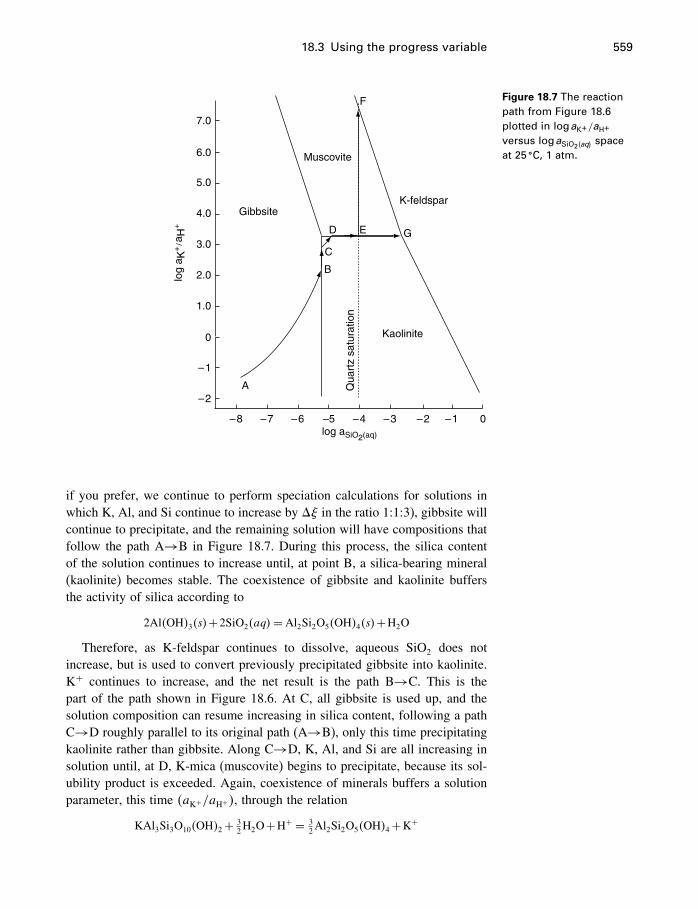
18.3 Using the progress variable 559
Figure 18.7 The reactionpath from Figure 18.6plotted in logaK+/aH+versus logaSiO2�aq�
spaceat 25 �C, 1 atm.
7.0
6.0
5.0
4.0
3.0
2.0
1.0
0
–1
–2
–8 –7 –6 –5 –4 –3 –2 –1 0
Kaolinite
GibbsiteK-feldspar
Muscovite
F
D E G
C
B
A Qua
rtz
satu
ratio
n
log aSiO2(aq)
log
a K+
/aH
+
if you prefer, we continue to perform speciation calculations for solutions inwhich K, Al, and Si continue to increase by �� in the ratio 1:1:3), gibbsite willcontinue to precipitate, and the remaining solution will have compositions thatfollow the path A→B in Figure 18.7. During this process, the silica contentof the solution continues to increase until, at point B, a silica-bearing mineral(kaolinite) becomes stable. The coexistence of gibbsite and kaolinite buffersthe activity of silica according to
2Al�OH�3�s�+2SiO2�aq�= Al2Si2O5�OH�4�s�+H2O
Therefore, as K-feldspar continues to dissolve, aqueous SiO2 does notincrease, but is used to convert previously precipitated gibbsite into kaolinite.K+ continues to increase, and the net result is the path B→C. This is thepart of the path shown in Figure 18.6. At C, all gibbsite is used up, and thesolution composition can resume increasing in silica content, following a pathC→D roughly parallel to its original path (A→B), only this time precipitatingkaolinite rather than gibbsite. Along C→D, K, Al, and Si are all increasing insolution until, at D, K-mica (muscovite) begins to precipitate, because its sol-ubility product is exceeded. Again, coexistence of minerals buffers a solutionparameter, this time �aK+/aH+�, through the relation
KAl3Si3O10�OH�2+ 32H2O+H+ = 3
2Al2Si2O5�OH�4+K+
560 Process modeling
Because the ratio �aK+/aH+� is fixed, but SiO2 continues to increase asK-feldspar dissolves, kaolinite reacts to form muscovite, and the solution fol-lows path D→E, at which point the solution becomes saturated with quartz,and if equilibrium is maintained, quartz will begin to precipitate. With fourcomponents (K2O, Al2O3, SiO2, H2O), a maximum of four phases can coexistat our arbitrarily chosen T and P (25 �C, 1 atm) according to the phase rule.With quartz, muscovite, kaolinite, and water, this number has now been reachedand cannot be exceeded (K-feldspar doesn’t count; it is being used as a sourceof solutes, and has not yet equilibrated with the solution). Therefore, if wecontinue to add K2O, Al2O3, and SiO2 from the K-feldspar to the solution, thesolution will stay at point E while kaolinite reacts with the solution to formmuscovite, and quartz continues to precipitate. When kaolinite is all used up,additional dissolution of K-feldspar will drive the solution composition alongE→F, with the SiO2 content of the solution buffered by the presence of quartz.At point F, K-feldspar finally becomes stable.
Alternatively, at point E, if quartz does not precipitate, the solution com-position could continue from E to G, where K-feldspar would also becomestable, but this time in a solution oversaturated with quartz. It would coexistmetastably with muscovite and kaolinite, rather than stably with muscovite andquartz. In nature, quartz quite often does not precipitate at low temperatures,and in computer calculations that simulate equilibrium, it can be preventedfrom “precipitating” by removing it from the list of minerals available to theprogram.
The numerical modelThe description of the reaction path given above is not just imagined; it is theresult of reaction path calculations similar in principle to the aragonite→calciteand iron oxidation examples we have already considered. However, theK-feldspar dissolution reaction is obviously a bit more complicated. For onething, the dissolution reaction considered in the calculations is not (18.48), butthe complete reaction involving all known species believed to be significant.This reaction obviously changes from time to time, as minerals appear anddisappear. For the path A→B in Figure 18.7, gibbsite is considered to bein equilibrium with the aqueous solution, all dissolved aqueous species areassumed to be equilibrated, and the dissolution reaction is
�KAlSi3O8KAlSi3O8+�H2O
H2O
→ �Al�OH�3Al�OH�3�gibbsite�
+�K+K++�Al3+Al3++�Al�OH�2+Al�OH�2++�Al�OH�−4 Al�OH�−4+�H4SiO4
H4SiO4+�H3SiO−4H3SiO
−4 +�H+H++�OH−OH−
(18.51)
where the quantities �i above are the stoichiometric coefficients of each species,but with the overbar added to indicate that they are not constants as before,
18.3 Using the progress variable 561
but variables to be calculated. Although the stoichiometric coefficients in eachelementary or individual reaction such as (18.49) are always integers, the overalldissolution reactions such as (18.51) are made up of numerous simultaneousindividual reactions, and the coefficients become nonintegral. Calculating themis part of the problem.
A convenient way to start would be to let the system contain 1000 g waterand assign �KAlSi3O8
= −1. Each �i then represents the rate of change in themolality of the subscripted species i with a reaction step d�:
dmid�
= �i (18.52)
which is analogous to Equation (18.8). To solve for each individual �i we need10 equations in the 10 unknowns �i, and these are provided by a combinationof equilibrium constant expressions and mass balances for K, Al, Si, O, andH. Solving these 10 equations using matrix algebra results in the 10 values of�i in (18.51), recalling that �KAlSi3O8
=−1. Then using
mi =m�i +�i �� (18.53)
which is equivalent to (18.29) and (18.30) in our aragonite→calcite example,and (18.39) in our iron-oxidation example. New concentrations of all aqueousspecies are calculated after each reaction increment, as well as new quantities ofany solids that are dissolving or precipitating. Inclusion of information on therelative reaction rates, often using the approximation afforded by transition statetheory for reactions with unknown rates, is easily done as shown in the iron-oxidation example. These calculations, plus calculation of all individual activitycoefficients, is repeated over and over (iteratively) until the final equilibriumstate is reached.
A useful introduction to modeling reaction paths is Steinmann et al. (1994).They show that the reaction path for K-feldspar dissolution as projected inlogaK+/aH+ versus logaSiO2�aq�
space is highly dependent on the starting solu-tion composition, and that with certain assumptions, the path can be calculatedusing a spreadsheet.
18.3.3 Comment
Clearly there is no theoretical limit to the complexity of the reactions that mightbe considered in this way. In addition, it is quite possible to couple this type ofcalculation with other types, such as fluid flow, heat flow, pressure changes,diffusion, permeability changes, deformation, and so on, because these othermodel calculations also are carried out iteratively in a large series of smallsteps. Thus, for example, after carrying out a �� step in a reaction path model,we could then take a small step in a heat flow model, then a small step in afluid flow model, and then return to the reaction model, and so on. The heat
562 Process modeling
flow calculation would depend on the results of the reaction path, because thereaction would be exo- or endothermic, and the fluid flow calculation woulddepend on any permeability changes caused by the chemical reactions, as wellas on viscosity changes caused by changes in temperature. Each model resultis dependent on all the others in a coupled fashion. Naturally, the demandson data, scientific insight, programming talent, and computer resources growsenormously with each additional factor to be modeled. This area is one ofconsiderable activity at the present time.
Why would we want to perform such complex calculations, especially whensome of them may be quite unrealistic? For example, we know that quasi-staticreactions are unrealistic, yet they are computed everywhere these days. Well,you could easily say that the equilibrium thermodynamic model is unrealistictoo, yet it is quite useful. Reaction path models are useful because they help usshape our ideas about what might be happening in natural processes. You neednot believe the results of such models in an absolute sense, but they usuallyreflect some or many aspects of what is really happening in the natural situationbeing simulated.
Besides, the game is not over. The comparison of model results with naturalsituations, and the improvement of the models to better simulate nature, isitself an iterative process, which will continue as long as we continue to beinterested in understanding the world around us. Most scientists believe thatif you can make a mathematical model of a situation, no matter how crude,you will understand that situation at a deeper level than if you just speculateabout it. Poincaré (1952) said “It is far better to predict without certainty, thannever to have predicted at all.” Model building is thus important, but it mustbe combined with careful observation of nature, whether in the laboratory or inthe field, otherwise it will be quite inappropriate and perhaps useless. It is quitepossible to calculate exact answers to real problems that are quite meaningless,no matter how clever the mathematics is.
18.4 Affinity and the progress variable
A striking feature of the reaction path calculations we have been consideringis that in a sense they are independent of the Gibbs energy, which we knowcontrols which way these reactions proceed. In other words, by changing thesign in equations like (18.25) and (18.26) we can use exactly the same methodsto change calcite into aragonite, graphite into diamond, or to form K-feldsparfrom the dissolved species in solution, like running a movie backwards. Toinvestigate this further, we must link the progress variable with the Gibbsenergy. The K-feldspar case is a little too complex, and the calcite–aragonitecase is too simple. We choose a system that has an equilibrium constant forone reaction, and a manageable number of species, the system N2–H2.
18.4 Affinity and the progress variable 563
18.4.1 Components and species again
Consider the two-component system N2–H2. Components N2 and H2 refer tothe result you would get if you analyzed the system for total nitrogen and totalhydrogen. The actual molecular form taken by each element in the system isirrelevant. However, N2 and H2 might also refer to the species in the system,i.e., diatomic nitrogen molecules and diatomic hydrogen molecules. In realsystems, species N2 and H2 combine to form ammonia,
N2�g�+3H2�g�= 2NH3�g� (18.54)
so that there are at least three major species. In many systems, there may beonly a few components, but dozens or hundreds of species.
Equation (4.65)
dG=−SdT +VdP+c∑i
�idni [4.65]
was derived for systems of c independent components. For example, in thetwo-component system N2–H2, c = 2, and the final term on the right sidewould be
�N2dnN2
+�H2dnH2
However, the equation can also be used with i representing some or all ofthe species in the system, rather than independent components, as long as thespecies are related to one another in balanced chemical reactions, such thatthe number of independent compositional parameters remains equal to c. Thusthe final term on the right side of (4.65) could also read
�N2dnN2
+�H2dnH2
+�NH3dnNH3
where N2 and H2 are now species and not components. Although we nowhave three compositional terms, we also have an equation (18.54) relating them(assuming equilibrium), so there are still only two independent compositionalterms.
Changing from components to species in this way provides for some flexi-bility we shall take advantage of shortly. In a closed system, we cannot changethe chemical potentials of components N2 and H2, and the last term in (4.65)is zero. However, the chemical potentials of the species in (18.54) can changein a closed system, if the reaction progresses to the left or the right from somemetastable state towards the stable equilibrium state. The last term in (4.65)
(which would look a bit different in havings∑i=1
rather thanc∑i=1
, that is, s species
rather than c components) would not be zero, even in a closed system, if we
564 Process modeling
were considering chemical reactions progressing towards equilibrium. Further-more, in such cases this last term must always be negative, no matter in whichdirection the reaction proceeds, to be consistent with dGT�P ≤ 0. One otherthing to note is that, although in this case there is one reaction and three species,in other cases you may be considering one out of many simultaneous reactions,and many species. In these cases, all possible reactions must be proceedingtowards equilibrium at each increment of �, not just the one you happen to beconsidering.
18.4.2 The affinity
Considering a system at constant T and P, Equation (4.65) now shows that
dGT�P =s∑i=1
�idni (18.55)
where the i are not the c independent components, but the s species we areconsidering which form from those components. In our ammonia example,Equation (18.54), s = 3. Into this we substitute the relation dni = �id� from(18.8), to get
dGT�P =s∑i=1
��i�i�d� (18.56)
Comparing this to (4.46),
dG=−SdT +VdP−�d� [4.46]
we see that another definition of the affinity is
�=−s∑i
�i�i (18.57)
Recalling that our �i are positive for products and negative for reactants, thequantity
∑i �i�i is simply the difference in partial molar Gibbs energy between
products and reactants. For (18.5) this is
�3�C+4�D�︸ ︷︷ ︸products
− ��A+2�B�︸ ︷︷ ︸reactants
(18.58)
If this sum is zero, the reaction is at stable equilibrium, there is no third con-straint, the affinity is zero, the third term on the right side of (4.46) disappears,and both
dG=−SdT +VdP
and (4.40)
dG=−S dT +V dP [4.40]
apply to the (closed) system. If some constraint prevents reaction (18.5) fromproceeding to equilibrium, then the sum in (18.58) is not zero, but may be
18.4 Affinity and the progress variable 565
positive or negative, depending on whether (18.5) wants to go to the left orright. If the sum
∑i �i�i is positive (� negative), the reaction wants to go to
the left as written, d� is negative, and �d� is positive. If the sum is negative(� positive), the reaction proceeds to the right, d� is positive, and �d� ispositive. So �d� is inherently positive (or zero), and dGT�P is inherentlynegative for a spontaneous reaction, consistent with (from 4.46)
dGT�P =−�d� (18.59)
Equation (18.57) shows that the affinity is a ��T�P term, giving the“distance” in G between stable and metastable equilibrium surfaces, or states,and the amount of useful work that a chemical reaction can do as it reachesequilibrium. It is in fact represented by the vector A→ A′ in Figures 4.9band 18.2. It might be worth noting, too, that the units of � are moles, of� are Jmol−1, and so the Gibbs energy in equations such as (18.59) is thetotal, not the molar, Gibbs energy. As mentioned above, a common modelingpractice is to define the system as containing one kilogram of water, so that allmole numbers (ni) become molalities (mi).
18.4.3 Ammonia formation example
Now we can consider the formation of ammonia from hydrogen and nitrogen(reaction 18.54) patterned after a similar presentation in Denbigh (1981, §4.3).Consider a system at T and one bar consisting of one mole of pure N2 andthree moles of pure H2 kept separate from one another. This system has fourconstraints. In addition to T and P (the only constraints needed to define stableequilibrium), a third constraint is the separation of the gases, and the fourth is aconstraint on the reaction to form NH3. We release one constraint by allowingthe gases to mix, resulting in a metastable gaseous solution of N2 and H2.Then we allow reaction (18.54) to take place in the forward direction in 10increments, from pure N2+3H2 to two moles of pure NH3. Thus dnNH3
/d�= 2,and � increases from 0 to 1.0 during the reaction. After each increment ofreaction, nN2
= �1− ��, nH2= 3�1− ��, and nNH3
= 2�. The total number ofmoles in the system at any stage is
nN2+nH2
+nNH3= �1−��+ �3−3��+ �2��= 4−2�
and the mole fractions are
xN2= 1−�
4−2�
xH2= 3−3�
4−2�
xNH3= 2�
4−2�
⎫⎪⎪⎪⎪⎪⎪⎪⎬⎪⎪⎪⎪⎪⎪⎪⎭(18.60)
566 Process modeling
The goal is to minimize an expression for the Gibbs energy of this solution, sostarting with expressions from Chapter 7,
�mixGideal sol’n =Gideal sol’n−∑i
xiG�i [7.19]
= RT∑i
xi ln xi [7.20]
we write
Gideal sol’n =∑i
xiG�i +RT
∑i
xi ln xi (18.61)
In the present case, this becomes (for pure substances G� = ��)
Gideal sol’n = xN2��
N2+xH2
��H2
+xNH3��
NH3
+RT�xN2ln xN2
+xH2ln xH2
+xNH3ln xNH3
� (18.62)
To convert molar G to the total G of the solution, we multiply both sides bythe denominator of the mole fraction term, �4−2��, so
Gideal sol’n = nN2��
N2+nH2
��H2
+nNH3��
NH3
+RT�nN2ln xN2
+nH2ln xH2
+nNH3ln xNH3
� (18.63)
Substituting for ni,
Gideal sol’n = �1−����N2
+ �3−3����H2
+2���NH3
+RT��1−�� ln xN2+ �3−3�� ln xH2
+2� ln xNH3�
= ���N2
+3��H2�+��2��
NH3−��
N2−3��
H2�
+RT��1−�� ln xN2+ �3−3�� ln xH2
+2� ln xNH3� (18.64)
so
Gideal sol’n− ���N2
+3��H2�= ���r���+RT��1−�� ln xN2
+ �3−3�� ln xH2+2� ln xNH3
�
= ���r���+�mixG
(18.65)
where G is the total Gibbs energy of the system containing �4−2�� moles ofnitrogen, hydrogen and ammonia gases, assuming ideality, �r�
� is the standardGibbs energy of reaction (18.54) at T from supcrt92, and � is the progressvariable which can have any value between 0 and 1.0. Note that the RT� �term is simply the total energy form of (7.20), and can be called �mixG, thetotal Gibbs energy of mixing. All we have done is to convert Equation (18.61)
18.4 Affinity and the progress variable 567
Reaction deltas – d, � and �
On page 29 we looked at the meaning of �rV�, the value of which changes
depending on how you write the reaction, and in §3.4.1, page 38, we used
differential notation where we could easily have used delta notation. For example,
we wrote w = mg ·dh where we could just as easily have written w = mg ·�h.Because there is a persistent tendency to see differentials as infinitesimals, we
made the point that dh is not necessarily infinitesimal, so in a sense we have not
changed anything in switching from � to d. What we said there is true enough,
but it is not the whole story.
� is a scalar difference between any two quantities. It could be the difference
in weight of two rock specimens. A differential dx, on the other hand, although
it need not be infinitesimal (see Figure C.1), is not just the difference between
any two quantities called x. It means that there is a mathematical function for
which it represents some increment in the x variable. Therefore dGT�P = 0 has a
significantly different meaning than�GT�P = 0. dGT�P = 0 signifies the extremum
of a mathematical function, while �GT�P = 0 does not.
Another point that is sometimes made about “delta notation” is that it is commonly
used in two different ways (MacDonald, 1990; Spencer, 1973). One way is the
scalar difference just mentioned, as in describing the difference in V , G, etc.,
between two equilibrium states; for example, before and after the expansion of a
gas. The other is in using the progress variable, as in(�G��
)T�P
=−a�A−b�B+ c�C+d�D
= �� or, sometimes, �G
which is the application of Equation (18.59) to reaction (18.1). The point is that
in this case � refers to the slope of the G versus � curve, the instantaneous
rate of change of G. To eliminate the supposed confusion, a different symbol is
recommended for this usage, such as � or �, so that Equation (9.8) would become
�G= �G� +RT lnQ [MacDonald, 1990, Equation (4)]
This appears to be an idea whose time has not yet come.
into Equation (18.65) by switching to total Gibbs energy and introducing ourvariable mole fractions (18.60).
Evidently we can plot values of [G−���N2+3��
H2�] as a function of reaction
progress at various T s, and because the two �� terms are constants, the curvewill show the true shape of the Gibbs energy variation and the minimum atthe equilibrium value of �. Recall that � = 0 means a solution of one mole
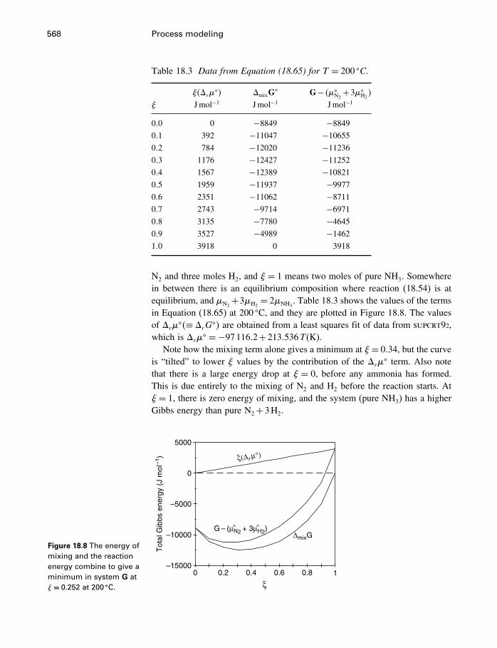
568 Process modeling
Table 18.3 Data from Equation (18.65) for T = 200 �C.
���r��� �mixG
� G− ���N2
+3��H2�
� Jmol−1 Jmol−1 Jmol−1
0�0 0 −8849 −8849
0�1 392 −11047 −10655
0�2 784 −12020 −11236
0�3 1176 −12427 −11252
0�4 1567 −12389 −10821
0�5 1959 −11937 −9977
0�6 2351 −11062 −8711
0�7 2743 −9714 −6971
0�8 3135 −7780 −4645
0�9 3527 −4989 −1462
1�0 3918 0 3918
N2 and three moles H2, and � = 1 means two moles of pure NH3. Somewherein between there is an equilibrium composition where reaction (18.54) is atequilibrium, and �N2
+3�H2= 2�NH3
. Table 18.3 shows the values of the termsin Equation (18.65) at 200 �C, and they are plotted in Figure 18.8. The valuesof �r�
��≡ �rG�� are obtained from a least squares fit of data from supcrt92,
which is �r�� = −97116�2+213�536T (K).
Note how the mixing term alone gives a minimum at �= 0�34, but the curveis “tilted” to lower � values by the contribution of the �r�
� term. Also notethat there is a large energy drop at � = 0, before any ammonia has formed.This is due entirely to the mixing of N2 and H2 before the reaction starts. At� = 1, there is zero energy of mixing, and the system (pure NH3) has a higherGibbs energy than pure N2+3H2.
Figure 18.8 The energy ofmixing and the reactionenergy combine to give aminimum in system G at� = 0�252 at 200 �C.
5000
0
0 0.2 0.4 0.6 0.8 1
–5000
–10000
–15000
Tot
al G
ibbs
ene
rgy
(J m
ol–1
)
∆mixGG – (µN2 + 3µH2)
ξ(∆r µ°)
ξ
° °
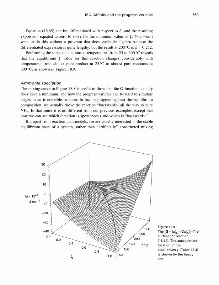
18.4 Affinity and the progress variable 569
Equation (18.65) can be differentiated with respect to �, and the resultingexpression equated to zero to solve for the minimum value of �. You won’twant to do this without a program that does symbolic algebra because thedifferentiated expression is quite lengthy, but the result at 200 �C is � = 0�252.
Performing the same calculations at temperatures from 25 to 300 �C revealsthat the equilibrium � value for this reaction changes considerably withtemperature, from almost pure product at 25 �C to almost pure reactants at300 �C, as shown in Figure 18.9.
Ammonia speciationThe mixing curve in Figure 18.8 is useful to show that the G function actuallydoes have a minimum, and how the progress variable can be used to simulatestages in an irreversible reaction. In fact in progressing past the equilibriumcomposition, we actually drove the reaction “backwards” all the way to pureNH3. In that sense it is no different from our previous examples, except thatnow we can see which direction is spontaneous and which is “backwards.”
But apart from reaction path models, we are usually interested in the stableequilibrium state of a system, rather than “artificially” constructed mixing
30
20
10
0G × 10–3
J mol–1
T °C
–10
–20
–30
–40
0.00.2
0.40.6
0.8
01.0 50
100
150
200
250300
ξ
Figure 18.9The G− ���
N2+3��
H2�–T –�
surface for reaction(18.54). The approximatelocation of theequilibrium � (Table 18.4)is shown by the heavyline.
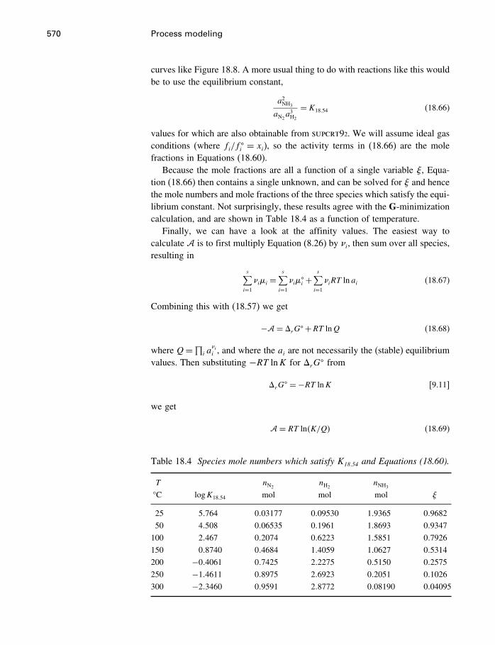
570 Process modeling
curves like Figure 18.8. A more usual thing to do with reactions like this wouldbe to use the equilibrium constant,
a2NH3
aN2a3H2
= K18�54 (18.66)
values for which are also obtainable from supcrt92. We will assume ideal gasconditions (where fi/f
�i = xi), so the activity terms in (18.66) are the mole
fractions in Equations (18.60).Because the mole fractions are all a function of a single variable �, Equa-
tion (18.66) then contains a single unknown, and can be solved for � and hencethe mole numbers and mole fractions of the three species which satisfy the equi-librium constant. Not surprisingly, these results agree with the G-minimizationcalculation, and are shown in Table 18.4 as a function of temperature.
Finally, we can have a look at the affinity values. The easiest way tocalculate � is to first multiply Equation (8.26) by �i, then sum over all species,resulting in
s∑i=1
�i�i =s∑i=1
�i��i +
s∑i=1
�iRT lnai (18.67)
Combining this with (18.57) we get
−�= �rG� +RT lnQ (18.68)
where Q=∏i a�ii , and where the ai are not necessarily the (stable) equilibrium
values. Then substituting −RT lnK for �rG� from
�rG� = −RT lnK [9.11]
we get
�= RT ln�K/Q� (18.69)
Table 18.4 Species mole numbers which satisfy K18�54 and Equations (18.60).
T nN2nH2
nNH3
°C logK18�54 mol mol mol �
25 5�764 0�03177 0�09530 1�9365 0�9682
50 4�508 0�06535 0�1961 1�8693 0�9347
100 2�467 0�2074 0�6223 1�5851 0�7926
150 0�8740 0�4684 1�4059 1�0627 0�5314
200 −0�4061 0�7425 2�2275 0�5150 0�2575
250 −1�4611 0�8975 2�6923 0�2051 0�1026
300 −2�3460 0�9591 2�8772 0�08190 0�04095
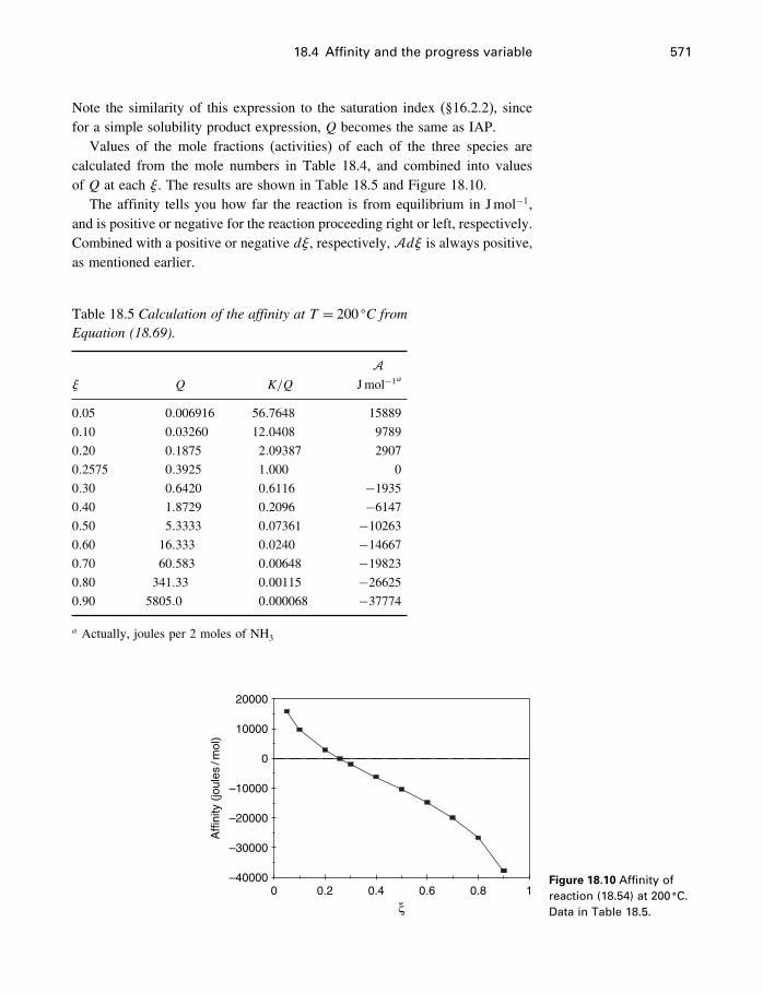
18.4 Affinity and the progress variable 571
Note the similarity of this expression to the saturation index (§16.2.2), sincefor a simple solubility product expression, Q becomes the same as IAP.
Values of the mole fractions (activities) of each of the three species arecalculated from the mole numbers in Table 18.4, and combined into valuesof Q at each �. The results are shown in Table 18.5 and Figure 18.10.
The affinity tells you how far the reaction is from equilibrium in Jmol−1,and is positive or negative for the reaction proceeding right or left, respectively.Combined with a positive or negative d�, respectively, �d� is always positive,as mentioned earlier.
Table 18.5 Calculation of the affinity at T = 200 �C fromEquation (18.69).
�
� Q K/Q Jmol−1a
0�05 0�006916 56�7648 15889
0�10 0�03260 12�0408 9789
0�20 0�1875 2�09387 2907
0�2575 0�3925 1�000 0
0�30 0�6420 0�6116 −1935
0�40 1�8729 0�2096 −6147
0�50 5�3333 0�07361 −10263
0�60 16�333 0�0240 −14667
0�70 60�583 0�00648 −19823
0�80 341�33 0�00115 −26625
0�90 5805�0 0�000068 −37774
a Actually, joules per 2 moles of NH3
20000
10000
0
–10000
–20000
–30000
–400000 0.2 0.4 0.6 0.8 1
ξ
Affi
nity
(jo
ules
/mol
)
Figure 18.10 Affinity ofreaction (18.54) at 200 �C.Data in Table 18.5.
572 Process modeling
In systems having several simultaneous reactions, affinities and progressvariables for each reaction as well as for the whole system may be calculated.Unfortunately, affinities of individual reactions in such systems are not relatedin any simple way to the order in which those reactions will reach equilibrium,due to the effects of reaction coupling (Helgeson, 1979). Similarly, although theaffinity is commonly used in theoretical expressions for reaction rate constants,it is never the only determining factor. Nevertheless, it is always a centralconcept in thinking about irreversible processes.
18.5 Final comment
We have emphasized in various places a point of view about thermodynamicswhich is fairly philosophical, which may also seem of not much use to someoneinterested in complex natural phenomena. That is the idea that in doing ourthermodynamic calculations, we are not really calculating the properties ofnatural systems, but properties of simplified models of these systems. Themodels are mathematical, and the properties and processes in the model includesome that have no counterpart in the real world. Nevertheless, model resultsare useful in understanding the real systems, if the models are properly orappropriately constructed. The calculations must satisfy stringent mathematicalrelationships, often giving them a gloss of certainty to the untrained eye, butactually they are of use only if the model they constitute is appropriate, i.e., if ithas some similarity to the problems of interest.
One reason that it is a good idea to make the distinction between our mod-els and reality is that our “explanations” of thermodynamics (and other exactsciences) are often in terms of mathematical planes, surfaces, tangents, andother even more abstract concepts. Students look at these explanations withunderstanding of a sort, but also with an underlying but usually unexpressedbafflement as to what these shining, unblemished, perfect, mathematical con-structs have to do with anything real. It is best to come to terms with this prob-lem by admitting that thermodynamics is in fact all about these mathematicalconstructs. It is not difficult to understand thermodynamics as the mathemat-ics of certain planes, surfaces, tangents, etc. The more difficult problem is tounderstand why these mathematical constructs have such direct relevance toour universe, but that is best left to the philosophers.
How do we assure ourselves that our models are appropriate? There is ofcourse no way to be sure. The construction of models useful in understand-ing nature is the essence of science and relies as much upon creativity andimagination as any painting or musical composition. Unfortunately, the modelsuse the language of mathematics, rather than shapes and colors or musicalnotes and are hence not understandable to anyone who does not know thelanguage. This is unfortunate, because mathematics and mathematical modelshave their own kind of beauty, which easily rivals that of the arts. Although
18.5 Final comment 573
we don’t know why the universe should be such that mathematics is so usefulin describing it, there is no doubt that it is useful. It seems clear that the moremathematical tools you have in your repertoire, the more adept you will be atfitting mathematics to your observations.
As mentioned in §18.3.3, the models being developed to simulate complexnatural phenomena are becoming very complex. Not only is it difficult to createsuch models, and to compile enough basic data to enable them to work, but itbecomes increasingly difficult to know how well they work. There is a greatdeal of uncertainty about what nature is actually doing, so that it’s often hardto know just how well model results coincide with natural observations. Thismeans that in understanding natural systems, insightful field observations arejust as important as model construction. And model results may turn out to bereasonably accurate, based on entirely incorrect ideas. Just because a model“works” does not mean it is right. All this means that there is plenty of scopefor thermodynamics and the tools built upon it in the years to come, in ourquest to understand our world and how it works.
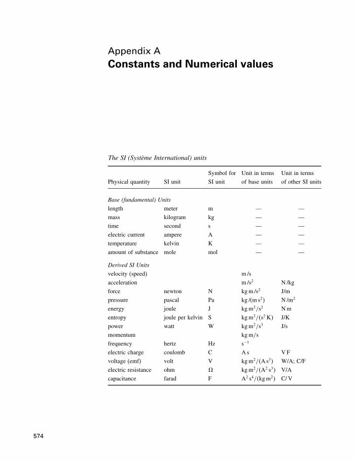
Appendix AConstants and Numerical values
The SI (Système International) units
Symbol for Unit in terms Unit in terms
Physical quantity SI unit SI unit of base units of other SI units
Base (fundamental) Units
length meter m — —
mass kilogram kg — —
time second s — —
electric current ampere A — —
temperature kelvin K — —
amount of substance mole mol — —
Derived SI Units
velocity (speed) m /s
acceleration m /s2 N /kg
force newton N kgm /s2 J/m
pressure pascal Pa kg /(m s2) N /m2
energy joule J kgm2/s2 Nm
entropy joule per kelvin S kgm2/�s2 K� J/K
power watt W kgm2/s3 J/s
momentum kgm/s
frequency hertz Hz s−1
electric charge coulomb C A s VF
voltage (emf) volt V kgm2/�As3� W/A; C/F
electric resistance ohm # kgm2/�A2 s3� V/A
capacitance farad F A2 s4/�kgm2� C/V
574
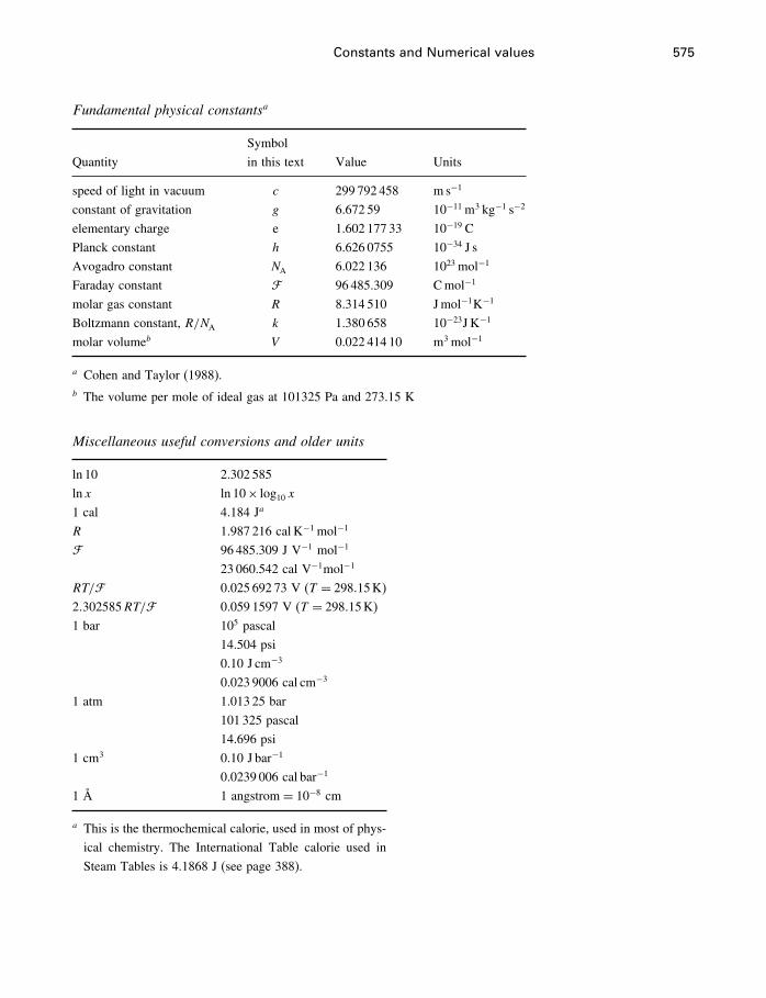
Constants and Numerical values 575
Fundamental physical constantsa
Symbol
Quantity in this text Value Units
speed of light in vacuum c 299 792 458 m s−1
constant of gravitation g 6.672 59 10−11 m3 kg−1 s−2
elementary charge e 1.602 177 33 10−19 C
Planck constant h 6.626 0755 10−34 J s
Avogadro constant NA 6.022 136 1023 mol−1
Faraday constant � 96 485.309 Cmol−1
molar gas constant R 8.314 510 Jmol−1K−1
Boltzmann constant, R/NA k 1.380 658 10−23J K−1
molar volumeb V 0.022 414 10 m3 mol−1
a Cohen and Taylor (1988).b The volume per mole of ideal gas at 101325 Pa and 273.15 K
Miscellaneous useful conversions and older units
ln 10 2.302 585
ln x ln 10× log10 x
1 cal 4.184 Ja
R 1.987 216 cal K−1 mol−1
� 96 485.309 J V−1 mol−1
23 060.542 cal V−1mol−1
RT/� 0.025 692 73 V (T = 298�15K)
2�302585RT/� 0.059 1597 V (T = 298�15K)
1 bar 105 pascal
14.504 psi
0.10 J cm−3
0.023 9006 cal cm−3
1 atm 1.013 25 bar
101 325 pascal
14.696 psi
1 cm3 0.10 J bar−1
0.0239 006 cal bar−1
1 Å 1 angstrom = 10−8 cm
a This is the thermochemical calorie, used in most of phys-
ical chemistry. The International Table calorie used in
Steam Tables is 4.1868 J (see page 388).
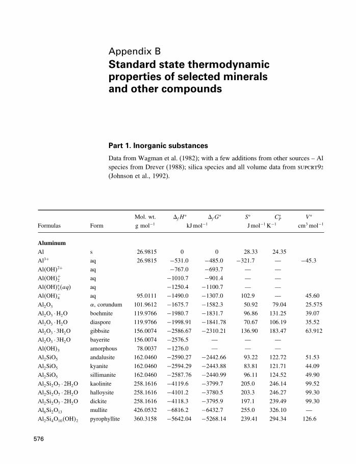
Appendix BStandard state thermodynamicproperties of selected mineralsand other compounds
Part 1. Inorganic substances
Data from Wagman et al. (1982); with a few additions from other sources – Alspecies from Drever (1988); silica species and all volume data from supcrt92(Johnson et al., 1992).
Mol. wt. �fH� �fG
� S� C�P V �
Formulas Form g mol−1 kJmol−1 Jmol−1 K−1 cm3 mol−1
AluminumAl s 26�9815 0 0 28�33 24�35
Al3+ aq 26�9815 −531�0 −485�0 −321�7 — −45�3
Al�OH�2+ aq −767�0 −693�7 — —
Al�OH�+2 aq −1010�7 −901�4 — —
Al�OH��3�aq� aq −1250�4 −1100�7 — —
Al�OH�−4 aq 95�0111 −1490�0 −1307�0 102�9 — 45�60
Al2O3 , corundum 101�9612 −1675�7 −1582�3 50�92 79�04 25�575
Al2O3 ·H2O boehmite 119�9766 −1980�7 −1831�7 96�86 131�25 39�07
Al2O3 ·H2O diaspore 119�9766 −1998�91 −1841�78 70�67 106�19 35�52
Al2O3 ·3H2O gibbsite 156�0074 −2586�67 −2310�21 136�90 183�47 63�912
Al2O3 ·3H2O bayerite 156�0074 −2576�5 — — —
Al�OH�3 amorphous 78�0037 −1276�0 — — —
Al2SiO5 andalusite 162�0460 −2590�27 −2442�66 93�22 122�72 51�53
Al2SiO5 kyanite 162�0460 −2594�29 −2443�88 83�81 121�71 44�09
Al2SiO5 sillimanite 162�0460 −2587�76 −2440�99 96�11 124�52 49�90
Al2Si2O7 ·2H2O kaolinite 258�1616 −4119�6 −3799�7 205�0 246�14 99�52
Al2Si2O7 ·2H2O halloysite 258�1616 −4101�2 −3780�5 203�3 246�27 99�30
Al2Si2O7 ·2H2O dickite 258�1616 −4118�3 −3795�9 197�1 239�49 99�30
Al6Si2O13 mullite 426�0532 −6816�2 −6432�7 255�0 326�10 —
Al2Si4O10�OH�2 pyrophyllite 360�3158 −5642�04 −5268�14 239�41 294�34 126�6
576
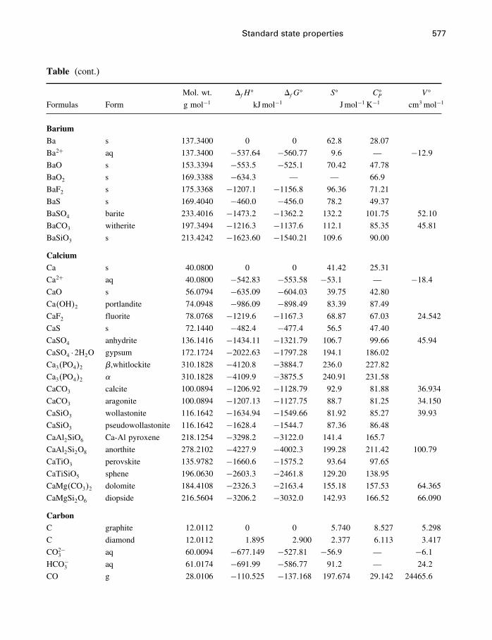
Standard state properties 577
Table (cont.)
Mol. wt. �fH� �fG
� S� C�P V �
Formulas Form g mol−1 kJmol−1 Jmol−1 K−1 cm3 mol−1
BariumBa s 137�3400 0 0 62�8 28�07
Ba2+ aq 137�3400 −537�64 −560�77 9�6 — −12�9
BaO s 153�3394 −553�5 −525�1 70�42 47�78
BaO2 s 169�3388 −634�3 — — 66�9
BaF2 s 175�3368 −1207�1 −1156�8 96�36 71�21
BaS s 169�4040 −460�0 −456�0 78�2 49�37
BaSO4 barite 233�4016 −1473�2 −1362�2 132�2 101�75 52�10
BaCO3 witherite 197�3494 −1216�3 −1137�6 112�1 85�35 45�81
BaSiO3 s 213�4242 −1623�60 −1540�21 109�6 90�00
CalciumCa s 40�0800 0 0 41�42 25�31
Ca2+ aq 40�0800 −542�83 −553�58 −53�1 — −18�4
CaO s 56�0794 −635�09 −604�03 39�75 42�80
Ca�OH�2 portlandite 74�0948 −986�09 −898�49 83�39 87�49
CaF2 fluorite 78�0768 −1219�6 −1167�3 68�87 67�03 24�542
CaS s 72�1440 −482�4 −477�4 56�5 47�40
CaSO4 anhydrite 136�1416 −1434�11 −1321�79 106�7 99�66 45�94
CaSO4 ·2H2O gypsum 172�1724 −2022�63 −1797�28 194�1 186�02
Ca3�PO4�2 �,whitlockite 310�1828 −4120�8 −3884�7 236�0 227�82
Ca3�PO4�2 310�1828 −4109�9 −3875�5 240�91 231�58
CaCO3 calcite 100�0894 −1206�92 −1128�79 92�9 81�88 36�934
CaCO3 aragonite 100�0894 −1207�13 −1127�75 88�7 81�25 34�150
CaSiO3 wollastonite 116�1642 −1634�94 −1549�66 81�92 85�27 39�93
CaSiO3 pseudowollastonite 116�1642 −1628�4 −1544�7 87�36 86�48
CaAl2SiO6 Ca-Al pyroxene 218�1254 −3298�2 −3122�0 141�4 165�7
CaAl2Si2O8 anorthite 278�2102 −4227�9 −4002�3 199�28 211�42 100�79
CaTiO3 perovskite 135�9782 −1660�6 −1575�2 93�64 97�65
CaTiSiO5 sphene 196�0630 −2603�3 −2461�8 129�20 138�95
CaMg�CO3�2 dolomite 184�4108 −2326�3 −2163�4 155�18 157�53 64�365
CaMgSi2O6 diopside 216�5604 −3206�2 −3032�0 142�93 166�52 66�090
CarbonC graphite 12�0112 0 0 5�740 8�527 5�298
C diamond 12�0112 1�895 2�900 2�377 6�113 3�417
CO2−3 aq 60�0094 −677�149 −527�81 −56�9 — −6�1
HCO−3 aq 61�0174 −691�99 −586�77 91�2 — 24�2
CO g 28�0106 −110�525 −137�168 197�674 29�142 24465�6
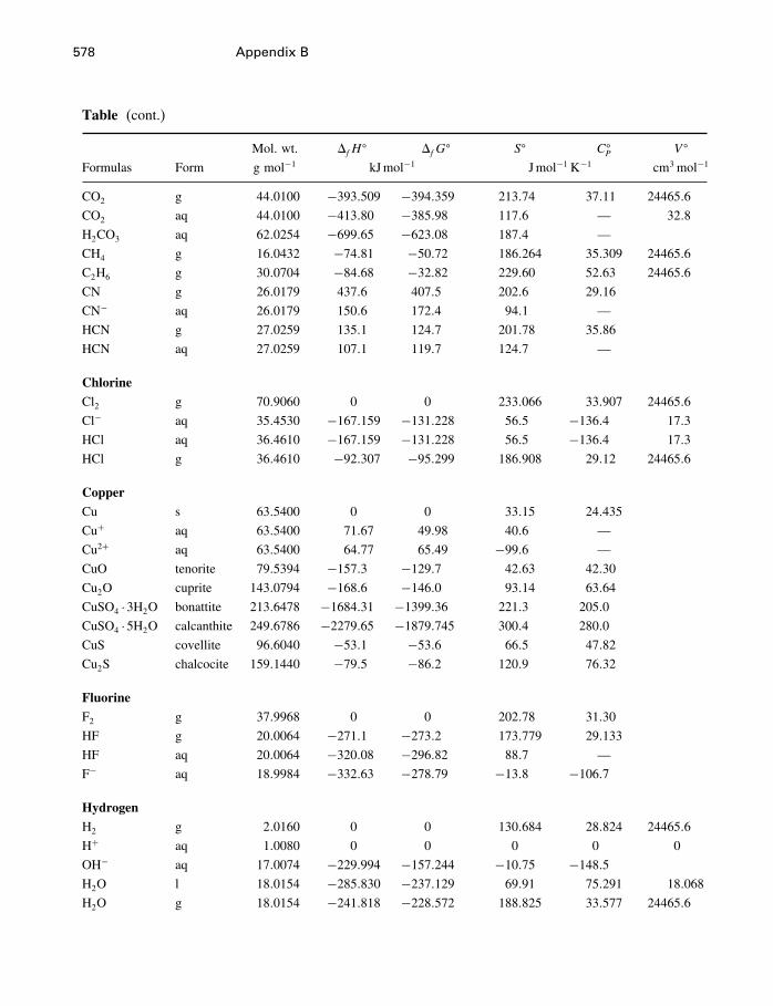
578 Appendix B
Table (cont.)
Mol. wt. �fH� �fG
� S� C�P V �
Formulas Form g mol−1 kJmol−1 Jmol−1 K−1 cm3 mol−1
CO2 g 44�0100 −393�509 −394�359 213�74 37�11 24465�6
CO2 aq 44�0100 −413�80 −385�98 117�6 — 32�8
H2CO3 aq 62�0254 −699�65 −623�08 187�4 —
CH4 g 16�0432 −74�81 −50�72 186�264 35�309 24465�6
C2H6 g 30�0704 −84�68 −32�82 229�60 52�63 24465�6
CN g 26�0179 437�6 407�5 202�6 29�16
CN− aq 26�0179 150�6 172�4 94�1 —
HCN g 27�0259 135�1 124�7 201�78 35�86
HCN aq 27�0259 107�1 119�7 124�7 —
ChlorineCl2 g 70�9060 0 0 233�066 33�907 24465�6
Cl− aq 35�4530 −167�159 −131�228 56�5 −136�4 17�3
HCl aq 36�4610 −167�159 −131�228 56�5 −136�4 17�3
HCl g 36�4610 −92�307 −95�299 186�908 29�12 24465�6
CopperCu s 63�5400 0 0 33�15 24�435
Cu+ aq 63�5400 71�67 49�98 40�6 —
Cu2+ aq 63�5400 64�77 65�49 −99�6 —
CuO tenorite 79�5394 −157�3 −129�7 42�63 42�30
Cu2O cuprite 143�0794 −168�6 −146�0 93�14 63�64
CuSO4 ·3H2O bonattite 213�6478 −1684�31 −1399�36 221�3 205�0
CuSO4 ·5H2O calcanthite 249�6786 −2279�65 −1879�745 300�4 280�0
CuS covellite 96�6040 −53�1 −53�6 66�5 47�82
Cu2S chalcocite 159�1440 −79�5 −86�2 120�9 76�32
FluorineF2 g 37�9968 0 0 202�78 31�30
HF g 20�0064 −271�1 −273�2 173�779 29�133
HF aq 20�0064 −320�08 −296�82 88�7 —
F− aq 18�9984 −332�63 −278�79 −13�8 −106�7
HydrogenH2 g 2�0160 0 0 130�684 28�824 24465�6
H+ aq 1�0080 0 0 0 0 0
OH− aq 17�0074 −229�994 −157�244 −10�75 −148�5
H2O l 18�0154 −285�830 −237�129 69�91 75�291 18�068
H2O g 18�0154 −241�818 −228�572 188�825 33�577 24465�6
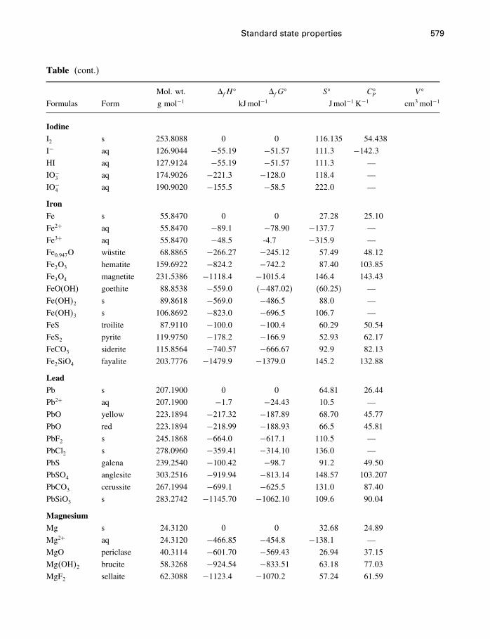
Standard state properties 579
Table (cont.)
Mol. wt. �fH� �fG
� S� C�P V �
Formulas Form g mol−1 kJmol−1 Jmol−1 K−1 cm3 mol−1
IodineI2 s 253�8088 0 0 116�135 54�438
I− aq 126�9044 −55�19 −51�57 111�3 −142�3
HI aq 127�9124 −55�19 −51�57 111�3 —
IO−3 aq 174�9026 −221�3 −128�0 118�4 —
IO−4 aq 190�9020 −155�5 −58�5 222�0 —
IronFe s 55�8470 0 0 27�28 25�10
Fe2+ aq 55�8470 −89�1 −78�90 −137�7 —
Fe3+ aq 55�8470 −48�5 -4.7 −315�9 —
Fe0�947O wüstite 68�8865 −266�27 −245�12 57�49 48�12
Fe2O3 hematite 159�6922 −824�2 −742�2 87�40 103�85
Fe3O4 magnetite 231�5386 −1118�4 −1015�4 146�4 143�43
FeO(OH) goethite 88�8538 −559�0 �−487�02� �60�25� —
Fe�OH�2 s 89�8618 −569�0 −486�5 88�0 —
Fe�OH�3 s 106�8692 −823�0 −696�5 106�7 —
FeS troilite 87�9110 −100�0 −100�4 60�29 50�54
FeS2 pyrite 119�9750 −178�2 −166�9 52�93 62�17
FeCO3 siderite 115�8564 −740�57 −666�67 92�9 82�13
Fe2SiO4 fayalite 203�7776 −1479�9 −1379�0 145�2 132�88
LeadPb s 207�1900 0 0 64�81 26�44
Pb2+ aq 207�1900 −1�7 −24�43 10�5 —
PbO yellow 223�1894 −217�32 −187�89 68�70 45�77
PbO red 223�1894 −218�99 −188�93 66�5 45�81
PbF2 s 245�1868 −664�0 −617�1 110�5 —
PbCl2 s 278�0960 −359�41 −314�10 136�0 —
PbS galena 239�2540 −100�42 −98�7 91�2 49�50
PbSO4 anglesite 303�2516 −919�94 −813�14 148�57 103�207
PbCO3 cerussite 267�1994 −699�1 −625�5 131�0 87�40
PbSiO3 s 283�2742 −1145�70 −1062�10 109�6 90�04
MagnesiumMg s 24�3120 0 0 32�68 24�89
Mg2+ aq 24�3120 −466�85 −454�8 −138�1 —
MgO periclase 40�3114 −601�70 −569�43 26�94 37�15
Mg�OH�2 brucite 58�3268 −924�54 −833�51 63�18 77�03
MgF2 sellaite 62�3088 −1123�4 −1070�2 57�24 61�59
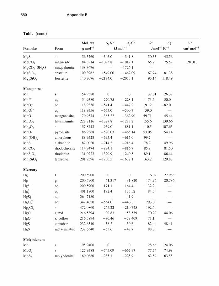
580 Appendix B
Table (cont.)
Mol. wt. �fH� �fG
� S� C�P V �
Formulas Form g mol−1 kJmol−1 Jmol−1 K−1 cm3 mol−1
MgS s 56�3760 −346�0 −341�8 50�33 45�56
MgCO3 magnesite 84�3214 −1095�8 −1012�1 65�7 75�52 28�018
MgCO3 ·3H2O nesquehonite 138�3676 — −1726�1 — —
MgSiO3 enstatite 100�3962 −1549�00 −1462�09 67�74 81�38
Mg2SiO4 forsterite 140�7076 −2174�0 −2055�1 95�14 118�49
ManganeseMn s 54�9380 0 0 32�01 26�32
Mn2+ aq 54�9380 −220�75 −228�1 −73�6 50�0
MnO−4 aq 118�9356 −541�4 −447�2 191.2 −82�0
MnO2−4 aq 118�9356 −653�0 −500�7 59.0 —
MnO manganosite 70�9374 −385�22 −362�90 59.71 45�44
Mn3O4 hausmannite 228�8116 −1387�8 −1283�2 155.6 139�66
Mn2O3 s 157�8742 −959�0 −881�1 110.5 107�65
MnO2 pyrolusite 86�9368 −520�03 −465�14 53.05 54�14
Mn�OH�2 amorphous 88�9528 −695�4 −615�0 99.2 —
MnS alabandite 87�0020 −214�2 −218�4 78.2 49�96
MnCO3 rhodochrosite 114�9474 −894�1 −816�7 85.8 81�50
MnSiO3 rhodonite 131�0222 −1320�9 −1240�5 89.1 86�44
Mn2SiO4 tephroite 201�9596 −1730�5 −1632�1 163.2 129�87
MercuryHg l 200�5900 0 0 76�02 27�983
Hg g 200�5900 61�317 31�820 174�96 20�786
Hg2+ aq 200�5900 171�1 164�4 −32�2 —
Hg2+2 aq 401�1800 172�4 153�52 84�5 —
HgS2−2 aq 264�7180 — 41�9 — —
HgCl2−4 aq 342�4020 −554�0 −446�8 293�0 —
Hg2Cl2 s 472�0860 −265�22 −210�745 192�5 —
HgO s, red 216�5894 −90�83 −58�539 70�29 44�06
HgO s, yellow 216�5894 −90�46 −58�409 71�1 —
HgS cinnabar 232�6540 −58�2 −50�6 82�4 48�41
HgS metacinnabar 232�6540 −53�6 −47�7 88�3 —
MolybdenumMo s 95�9400 0 0 28�66 24�06
MoO3 s 127�9388 −745�09 −667�97 77�74 74�98
MoS2 molybdenite 160�0680 −235�1 −225�9 62�59 63�55
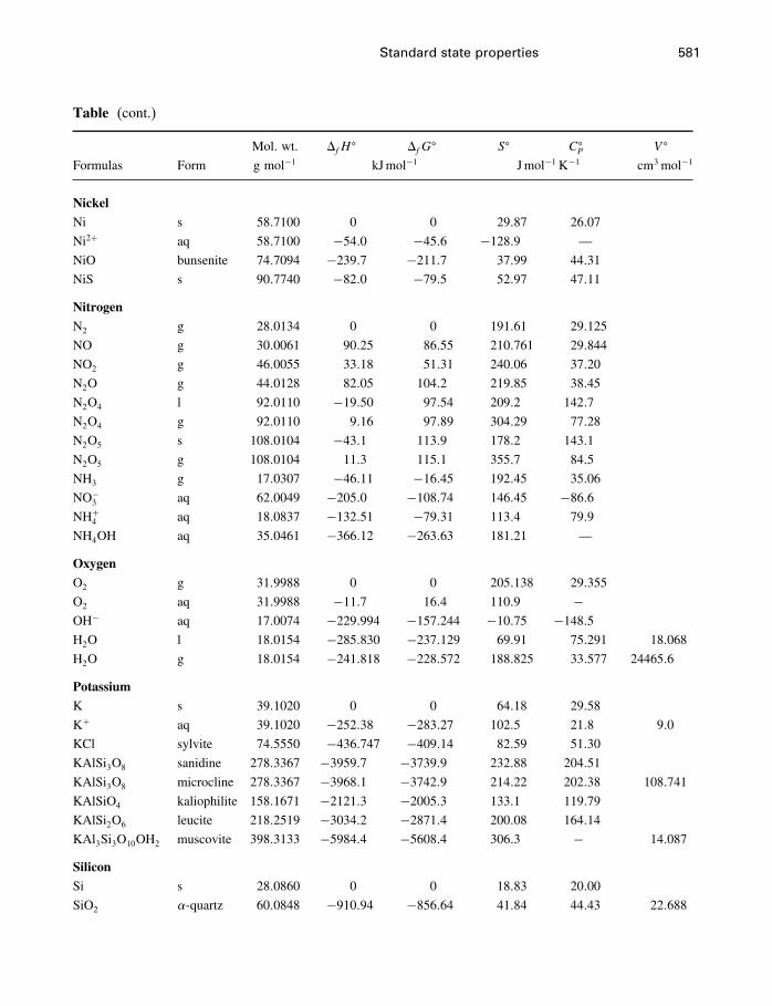
Standard state properties 581
Table (cont.)
Mol. wt. �fH� �fG
� S� C�P V �
Formulas Form g mol−1 kJmol−1 Jmol−1 K−1 cm3 mol−1
NickelNi s 58�7100 0 0 29�87 26�07
Ni2+ aq 58�7100 −54�0 −45�6 −128�9 —
NiO bunsenite 74�7094 −239�7 −211�7 37�99 44�31
NiS s 90�7740 −82�0 −79�5 52�97 47�11
NitrogenN2 g 28�0134 0 0 191�61 29�125
NO g 30�0061 90�25 86�55 210�761 29�844
NO2 g 46�0055 33�18 51�31 240�06 37�20
N2O g 44�0128 82�05 104�2 219�85 38�45
N2O4 l 92�0110 −19�50 97�54 209�2 142�7
N2O4 g 92�0110 9�16 97�89 304�29 77�28
N2O5 s 108�0104 −43�1 113�9 178�2 143�1
N2O5 g 108�0104 11�3 115�1 355�7 84�5
NH3 g 17�0307 −46�11 −16�45 192�45 35�06
NO−3 aq 62�0049 −205�0 −108�74 146�45 −86�6
NH+4 aq 18�0837 −132�51 −79�31 113�4 79�9
NH4OH aq 35�0461 −366�12 −263�63 181�21 —
OxygenO2 g 31�9988 0 0 205�138 29�355
O2 aq 31�9988 −11�7 16�4 110�9 −OH− aq 17�0074 −229�994 −157�244 −10�75 −148�5
H2O l 18�0154 −285�830 −237�129 69�91 75�291 18�068
H2O g 18�0154 −241�818 −228�572 188�825 33�577 24465�6
PotassiumK s 39�1020 0 0 64�18 29�58
K+ aq 39�1020 −252�38 −283�27 102�5 21�8 9�0
KCl sylvite 74�5550 −436�747 −409�14 82�59 51�30
KAlSi3O8 sanidine 278�3367 −3959�7 −3739�9 232�88 204�51
KAlSi3O8 microcline 278�3367 −3968�1 −3742�9 214�22 202�38 108�741
KAlSiO4 kaliophilite 158�1671 −2121�3 −2005�3 133�1 119�79
KAlSi2O6 leucite 218�2519 −3034�2 −2871�4 200�08 164�14
KAl3Si3O10OH2 muscovite 398�3133 −5984�4 −5608�4 306�3 − 14�087
SiliconSi s 28�0860 0 0 18�83 20�00
SiO2 -quartz 60�0848 −910�94 −856�64 41�84 44�43 22�688
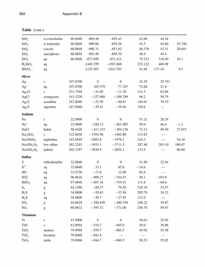
582 Appendix B
Table (cont.)
SiO2 -cristobalite 60�0848 -909�48 -855�43 42�68 44�18
SiO2 -tridymite 60�0848 -909�06 -855�26 43�5 44�60 25�740
SiO2 coesite 60�0848 -906�31 -851�62 40�376 43�51 20�641
SiO2 amorphous 60�0848 -903�49 -850�70 46�9 44�4
SiO2 aq 60�0848 -877�699 -833�411 75�312 318�40 16�1
H4SiO4 aq -1449�359 -1307�669 215�132 468�98
HSiO−3 aq -1125�583 -1013�783 41�84 -137�24 9�5
SilverAg s 107�8700 0 0 42�55 25�351
Ag+ aq 107�8700 105�579 77�107 72�68 21�8
Ag2O s 231�7394 −31�05 −11�20 121�3 65�86
AgCl cerargyrite 143�3230 −127�068 −109�789 96�2 50�79
Ag2S acanthite 247�8040 −32�59 −40�67 144�01 76�53
Ag2S argentite 247�8040 −29�41 −39�46 150�6 −SodiumNa s 22�9898 0 0 51�21 28�24
Na+ aq 22�9898 −240�12 −261�905 59�0 46�4 −1�2
NaCl halite 58�4428 −411�153 −384�138 72�13 50�50 27�015
Na2SiO3 s 122�0638 −1554�90 −1462�80 113�85 —
NaAlSiO4 nepheline 142�0549 −2092�8 −1978�1 124�3 — 54�16
NaAlSi3O8 low albite 262�2245 −3935�1 −3711�5 207�40 205�10 100�07
NaAlSi2O6 jadeite 202�1397 −3030�9 −2852�1 133�5 — 60�40
SulfurS orthorhombic 32�0640 0 0 31�80 22�64
S2− aq 32�0640 33�1 85�8 −14�6 —
HS− aq 33�0720 −17�6 12�08 62�8 —
SO2−4 aq 96�0616 −909�27 −744�53 20�1 −293�0
HSO−4 aq 97�0696 −887�34 −755�91 131�8 −84�0
S2 g 64�1280 128�37 79�30 228�18 32�47
H2S g 34�0800 −20�63 −33�56 205�79 34�23
H2S aq 34�0800 −39�7 −27�83 121�0 —
SO2 g 64�0628 −296�830 −300�194 248�22 39�87
SO3 g 80�0622 −395�72 −371�06 256�76 50�67
TitaniumTi s 47�9000 0 0 30�63 25�02
TiO s 63�8994 −519�7 −495�0 50�0 39�96
TiO2 anatase 79�8988 −939�7 −884�5 49�92 55�48
TiO2 brookite 79�8988 −941�8 — — —
TiO2 rutile 79�8988 −944�7 −889�5 50�33 55�02
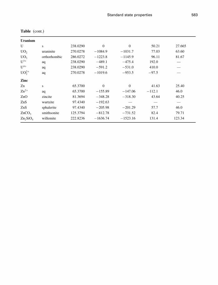
Standard state properties 583
Table (cont.)
UraniumU s 238�0290 0 0 50�21 27�665
UO2 uraninite 270�0278 −1084�9 −1031�7 77�03 63�60
UO3 orthorhombic 286�0272 −1223�8 −1145�9 96�11 81�67U3+ aq 238�0290 −489�1 −475�4 192�0 —
U4+ aq 238�0290 −591�2 −531�0 410�0 —
UO2+2 aq 270�0278 −1019�6 −953�5 −97�5 —
ZincZn s 65�3700 0 0 41�63 25�40
Zn2+ aq 65�3700 −155�89 −147�06 −112�1 46�0
ZnO zincite 81�3694 −348�28 −318�30 43�64 40�25
ZnS wurtzite 97�4340 −192�63 — — —
ZnS sphalerite 97�4340 −205�98 −201�29 57�7 46�0
ZnCO3 smithsonite 125�3794 −812�78 −731�52 82�4 79�71
Zn2SiO4 willemite 222�8236 −1636�74 −1523�16 131�4 123�34
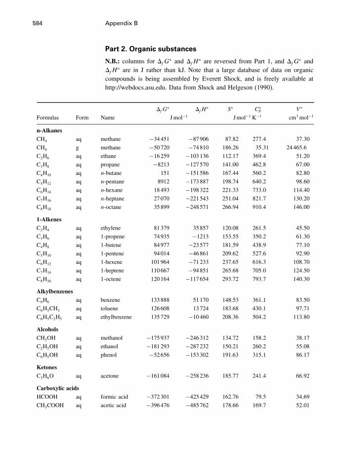
584 Appendix B
Part 2. Organic substances
N.B.: columns for �fG� and �fH
� are reversed from Part 1, and �fG� and
�fH� are in J rather than kJ. Note that a large database of data on organic
compounds is being assembled by Everett Shock, and is freely available athttp://webdocs.asu.edu. Data from Shock and Helgeson (1990).
�fG� �fH
� S� C�P V �
Formulas Form Name Jmol−1 Jmol−1 K−1 cm3 mol−1
n-AlkanesCH4 aq methane −34451 −87906 87.82 277�4 37�30
CH4 g methane −50720 −74810 186.26 35�31 24465�6
C2H6 aq ethane −16259 −103136 112.17 369�4 51�20
C3H8 aq propane −8213 −127570 141.00 462�8 67�00
C4H10 aq n-butane 151 −151586 167.44 560�2 82�80
C5H12 aq n-pentane 8912 −173887 198.74 640�2 98�60
C6H14 aq n-hexane 18493 −198322 221.33 733�0 114�40
C7H16 aq n-heptane 27070 −221543 251.04 821�7 130�20
C8H18 aq n-octane 35899 −248571 266.94 910�4 146�00
1-AlkenesC2H4 aq ethylene 81379 35857 120.08 261�5 45�50
C3H6 aq 1-propene 74935 −1213 153.55 350�2 61�30
C4H8 aq 1-butene 84977 −23577 181.59 438�9 77�10
C5H10 aq 1-pentene 94014 −46861 209.62 527�6 92�90
C6H12 aq 1-hexene 101964 −71233 237.65 616�3 108�70
C7H14 aq 1-heptene 110667 −94851 265.68 705�0 124�50
C8H16 aq 1-octene 120164 −117654 293.72 793�7 140�30
AlkylbenzenesC6H6 aq benzene 133888 51170 148.53 361�1 83�50
C6H5CH3 aq toluene 126608 13724 183.68 430�1 97�71
C6H5C2H5 aq ethylbenzene 135729 −10460 208.36 504�2 113�80
AlcoholsCH3OH aq methanol −175937 −246312 134.72 158�2 38�17
C2H5OH aq ethanol −181293 −287232 150.21 260�2 55�08
C6H5OH aq phenol −52656 −153302 191.63 315�1 86�17
KetonesC3H6O aq acetone −161084 −258236 185.77 241�4 66�92
Carboxylic acidsHCOOH aq formic acid −372301 −425429 162.76 79�5 34�69
CH3COOH aq acetic acid −396476 −485762 178.66 169�7 52�01
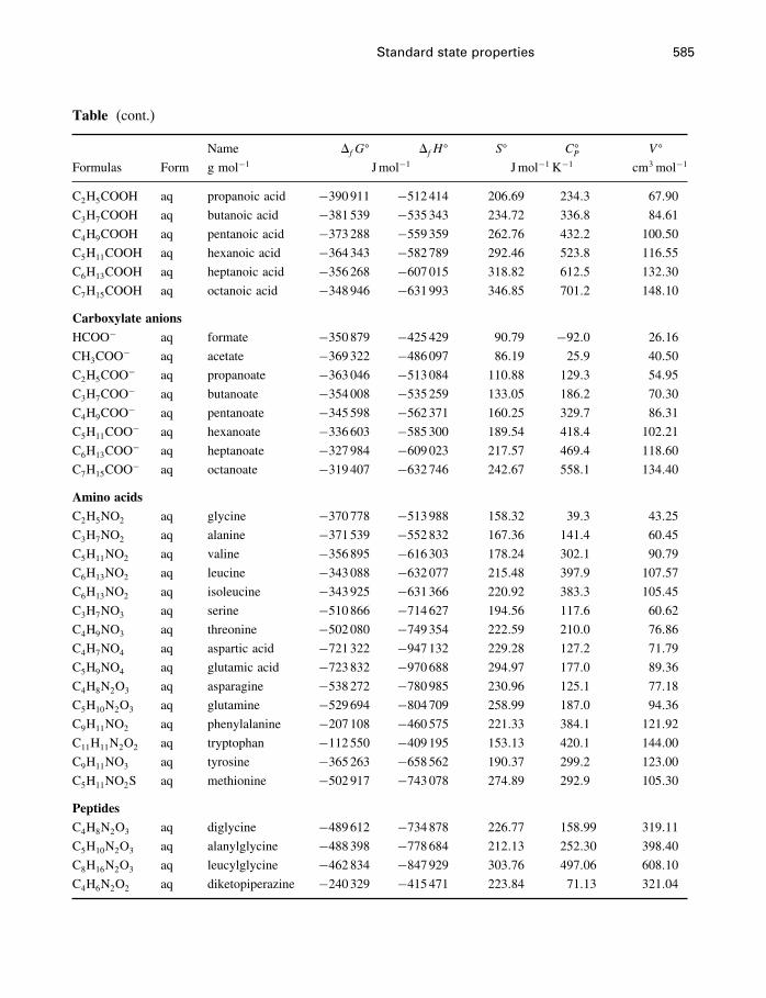
Standard state properties 585
Table (cont.)
Name �fG� �fH
� S� C�P V �
Formulas Form g mol−1 Jmol−1 Jmol−1 K−1 cm3 mol−1
C2H5COOH aq propanoic acid −390911 −512414 206�69 234�3 67�90
C3H7COOH aq butanoic acid −381539 −535343 234�72 336�8 84�61
C4H9COOH aq pentanoic acid −373288 −559359 262�76 432�2 100�50
C5H11COOH aq hexanoic acid −364343 −582789 292�46 523�8 116�55
C6H13COOH aq heptanoic acid −356268 −607015 318�82 612�5 132�30
C7H15COOH aq octanoic acid −348946 −631993 346�85 701�2 148�10
Carboxylate anionsHCOO− aq formate −350879 −425429 90�79 −92�0 26�16
CH3COO− aq acetate −369322 −486097 86�19 25�9 40�50
C2H5COO− aq propanoate −363046 −513084 110�88 129�3 54�95
C3H7COO− aq butanoate −354008 −535259 133�05 186�2 70�30
C4H9COO− aq pentanoate −345598 −562371 160�25 329�7 86�31
C5H11COO− aq hexanoate −336603 −585300 189�54 418�4 102�21
C6H13COO− aq heptanoate −327984 −609023 217�57 469�4 118�60
C7H15COO− aq octanoate −319407 −632746 242�67 558�1 134�40
Amino acidsC2H5NO2 aq glycine −370778 −513988 158�32 39�3 43�25
C3H7NO2 aq alanine −371539 −552832 167�36 141�4 60�45
C5H11NO2 aq valine −356895 −616303 178�24 302�1 90�79
C6H13NO2 aq leucine −343088 −632077 215�48 397�9 107�57
C6H13NO2 aq isoleucine −343925 −631366 220�92 383�3 105�45
C3H7NO3 aq serine −510866 −714627 194�56 117�6 60�62
C4H9NO3 aq threonine −502080 −749354 222�59 210�0 76�86
C4H7NO4 aq aspartic acid −721322 −947132 229�28 127�2 71�79
C5H9NO4 aq glutamic acid −723832 −970688 294�97 177�0 89�36
C4H8N2O3 aq asparagine −538272 −780985 230�96 125�1 77�18
C5H10N2O3 aq glutamine −529694 −804709 258�99 187�0 94�36
C9H11NO2 aq phenylalanine −207108 −460575 221�33 384�1 121�92
C11H11N2O2 aq tryptophan −112550 −409195 153�13 420�1 144�00
C9H11NO3 aq tyrosine −365263 −658562 190�37 299�2 123�00
C5H11NO2S aq methionine −502917 −743078 274�89 292�9 105�30
PeptidesC4H8N2O3 aq diglycine −489612 −734878 226�77 158�99 319�11
C5H10N2O3 aq alanylglycine −488398 −778684 212�13 252�30 398�40
C8H16N2O3 aq leucylglycine −462834 −847929 303�76 497�06 608�10
C4H6N2O2 aq diketopiperazine −240329 −415471 223�84 71�13 321�04
Appendix CSome mathematics
C.1 Essential mathematics
C.1.1 Differentials and derivatives
Figure C.1 illustrates the usual definition of a derivative. For any functiony = y�x�, the derivative of y, is a function y′�x� where
y′�x�= lim�x→0
(y�x+�x�−y�x�
�x
)(C.1)
As shown in Figure C.1, the quantity
y�x+�x�−y�x��x
is the slope of a line that intersects the function y�x� at two points, �x1� y1�and �x0� y0�, and �x = x1 − x0, �y = y1 − y0. As �x gets smaller, x1 and y1approach x0 and y0, and in the limit as �x→ 0, the line of intersection becomesthe tangent to y�x� at �x0� y0�. The notation y′�x� indicates that the derivative,or the slope of the tangent, is a new function of x, quite distinct from theoriginal function y�x��
If we let �x = dx and define dy, the differential of y, as
dy = y′�x�dx (C.2)
then
y′�x�= dy
dx(C.3)
and the symbol dy/dx is often used to represent the derivative. dx has alreadybeen defined as equal to �x, that is, any increment of x, and dy is a linear func-tion of dx as shown in Figure C.2. Obviously neither dx nor dy is necessarilyan infinitesimal quantity. It is an unfortunate fact that because dy/dx is equal tothe derivative, the concept of which involves allowing dx to become infinites-imally small, many students of thermodynamics get the idea that differentialsare infinitesimal quantities, and this is a stumbling block to the intuitive graspof the many equations involving differentials. During integration, of course,differentials can and do take on infinitesimal values.
586
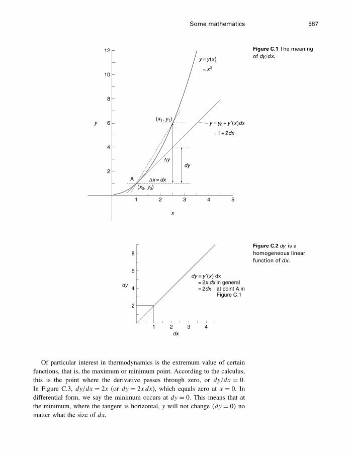
Some mathematics 587
12
10
8
6
4
2
y
y = y(x )
= x2
y = y0 + y ′(x )dx
= 1 + 2dx
(x1, y1)
(x0, y0)
∆ydy
∆x = dxA
x
1 2 3 4 5
Figure C.1 The meaningof dy/dx�
8
6
4
2
dy
dx1 2 3 4
dy = y ′(x ) dx = 2x dx in general = 2dx at point A in Figure C.1
Figure C.2 dy is ahomogeneous linearfunction of dx�
Of particular interest in thermodynamics is the extremum value of certainfunctions, that is, the maximum or minimum point. According to the calculus,this is the point where the derivative passes through zero, or dy/dx = 0.In Figure C.3, dy/dx = 2x (or dy = 2xdx), which equals zero at x = 0. Indifferential form, we say the minimum occurs at dy = 0. This means that atthe minimum, where the tangent is horizontal, y will not change �dy = 0� nomatter what the size of dx.
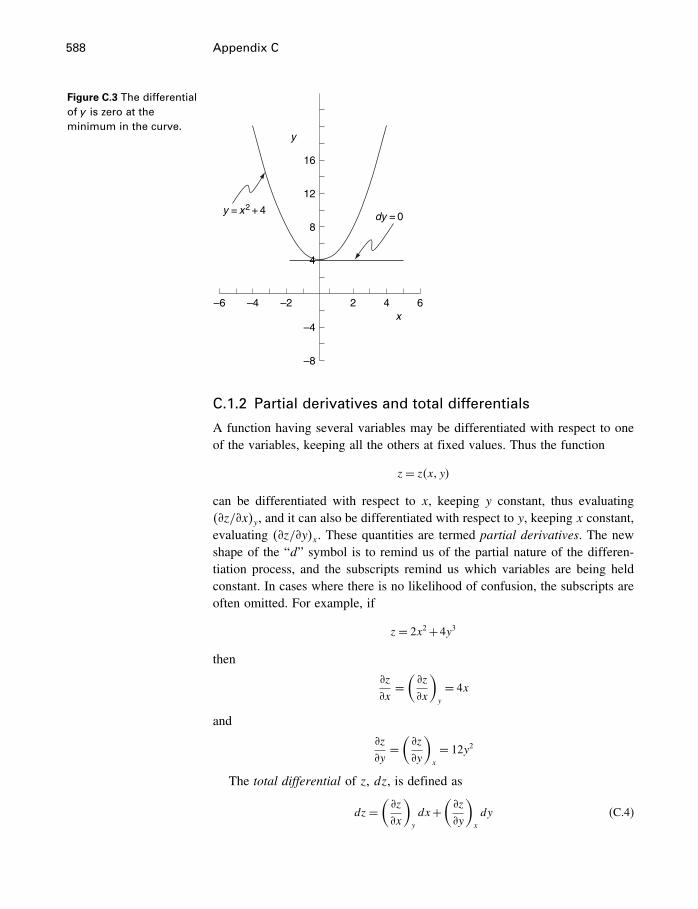
588 Appendix C
Figure C.3 The differentialof y is zero at theminimum in the curve.
y
x
16
12
8
4
–4
–8
2 4 6–6 –4 –2
y = x2 + 4dy = 0
C.1.2 Partial derivatives and total differentials
A function having several variables may be differentiated with respect to oneof the variables, keeping all the others at fixed values. Thus the function
z= z�x� y�
can be differentiated with respect to x, keeping y constant, thus evaluating��z/�x�y, and it can also be differentiated with respect to y, keeping x constant,evaluating ��z/�y�x. These quantities are termed partial derivatives. The newshape of the “d” symbol is to remind us of the partial nature of the differen-tiation process, and the subscripts remind us which variables are being heldconstant. In cases where there is no likelihood of confusion, the subscripts areoften omitted. For example, if
z= 2x2+4y3
then
�z
�x=(�z
�x
)y
= 4x
and
�z
�y=(�z
�y
)x
= 12y2
The total differential of z, dz, is defined as
dz=(�z
�x
)y
dx+(�z
�y
)x
dy (C.4)
Some mathematics 589
For example, if the function V = V�T�P� isV = RT
P(C.5)
where R is a constant, then
dV =(�V
�T
)P
dT +(�V
�P
)T
dP (C.6)
= R
PdT + −RT
P2dP (C.7)
Equation (C.4) has a very straightforward geometrical meaning, discussed inconnection with the fundamental equation in Chapter 4 (§4.6). Thermodynamicscommonly deals with continuous changes in multivariable systems. For thisreason, total differentials are frequently used, and it is essential to have a clearidea of their meaning.
C.1.3 Integration
Integration is the inverse of differentiation. That is, the problem is to find afunction when its rate of change is known. It is performed by summing up(functions of) differentials that are chosen to be very small (infinitesimals). Thiscan be done either in the general case, giving indefinite integrals, or betweenspecified limits, giving definite integrals. For example,∫
y′�x�dx = y�x�+ constant (C.8)
is the general case, since differentiation of y�x� plus any constant will givey′�x�, the derivative of a constant being zero.∫ b
ay′�x�dx = y�b�−y�a�
is the definite integral between the limits a and b and can be thought of as thearea under the curve y′�x� in the x–y plane, between the limits x= a and x= b.Both methods of integration have been used in applications of thermodynamicsin the Earth sciences, but generally speaking the definite integral is bettersuited to quantitative calculation. Variables are often said to be known “withina constant” or some similar phrase, which refers to a variable obtained fromthe indefinite integration of some function, as in Equation (C.8).
It is perhaps worthwhile to note here that the concept of infinitesimals,infinitely small increments, etc., remained mathematically unsatisfactory fora long time after Newton and Leibniz invented the calculus, and has beenlargely abandoned in the teaching of the calculus. These ideas have beensuperseded by the concept of limits. The continued and widespread use of theterm infinitesimal in the science literature seems to be a kind of shorthandway of referring to the process of limit-taking. It seems that scientists are notmuch bothered by many mathematical niceties which are of great concern tomathematicians.
590 Appendix C
C.2 Nonessential mathematics
C.2.1 Exact and inexact differentials
Exact differentials are those obtained by differentiating some continuous,single-valued function. Since the function can be obtained again by integration,exact differentials are expressions whose integrals will be the same no matterwhich path of integration is chosen. Accordingly, the total differentials wehave just discussed are also exact differentials. They are the “normal” kind ofdifferential. What then is an inexact differential?
Obviously if one always starts with a function and derives differentials fromit, one will never generate an inexact differential. However, in the physicalsciences one is apt to come across differential expressions of the type
M dx + N dy + · · · (C.9)
where M and N may or may not be functions of x and y. The concept ofinexact differentials arises because not every expression of this type (calleda Pfaff differential expression) is equal to the differential of some functionz= z�x� y�. For example, �xdy+ y dx� is clearly exact, being equal to d�xy�,but �xdy−y dx� is not equal to the differential of any function of x and y, andis inexact.
Expressions that are not exact (as well as those that are) are very importantin thermodynamics. (Note that we may speak of either dz or of M dx+N dyas being an exact differential, or of being exact.)
If M and/or N are not functions of x and y, the expression is inexact. IfM and N are functions of x and y, one may determine whether the expressionis exact (whether it is equal to the differential of some function of x and y)by determining whether M and N are the partial derivatives of some functionwith respect to x and y. If they are, then for the expression to be exact it isnecessary and sufficient that (
�M
�y
)x
=(�N
�x
)y
(C.10)
for all pairs of terms in the expression.Equation (C.10) is known as the reciprocity relation or cross-differentiation
identity. It follows from the fact that the order of differentiation of our originalfunction z= z�x� y� with respect to x and y is immaterial. Mathematically thisis written (
�
�y
(�z
�x
)y
)x
=(�
�x
(�z
�y
)x
)y
(C.11)
If, in Equation (C.9), M = ��z/�x�y and N = ��z/�y�x for some function z =z�x� y�, then Equation (C.10) must follow from (C.11).
Some mathematics 591
As an example of the use of this relation, let us test Equation (C.7) forexactness. Applying the reciprocity relation gives(
�
�T
(−RTP2
))P
=(�
�P
(R
P
))T
= −RP2
Hence Equation (C.6) has been shown to be an exact differential expression,as we knew it must be because we derived it by differentiating the functionV = RT/P�
Frankly, it is rarely of interest in thermodynamics to test expressions forexactness. The expressions in common use are generally well known to beexact or inexact. However, the reciprocity relationship is useful in derivingrelationships between thermodynamic variables.
Getting back to the inexact differentials, suppose we have an expression
Xdx+Y dy+Zdz (C.12)
where X, Y , and Z are functions of x, y, and z but reciprocity is not satisfied,1
and the expression is not exact. We may assign another variable to representthis expression, e.g.
� = Xdx+Y dy+Zdz
and this variable ��� is called an inexact differential. To remind ourselvesthat it represents a differential expression rather than an ordinary algebraicexpression, it is usually combined with some kind of letter “d” such as D or� or d– any form except d, which is reserved for exact differentials. Using �,we write
�� = Xdx+Y dy+Zdz
Inexact differentials such as �� are thus simply a shorthand notation fora differential expression such as (C.12) and are not the differential of anyfunction. It follows that they cannot be integrated without specifying a path.
Of special interest is the simplest of inexact differentials, y dx. When y andx are both independent variables, y dx is clearly inexact, since we may writethe equivalent expression y dx+0dy and applying the reciprocity relationship,(
�y
�y
)x
= 1 �=(�0�x
)y
Clearly there is no function the differential of which is equal to y dx. Similarly,not being exact, the integral of y dx is not independent of the path chosen. But
1 In the case of three or more terms, the reciprocity relation must hold between any two.
592 Appendix C
expressions like y dx are important in thermodynamics and must be integrated.The most common examples are P dV and T dS.
Expressions that are not exact can only be integrated after making themexact, and this is done by choosing a functional relationship between x and y,i.e., by making
y = y�x�
Now y and x are no longer independent of one another, and the expression
y�x�dx
is exact and may be integrated unambiguously. Reciprocity is satisfied sincewe may write y�x�dx as
y�x�dx+0dy
and (�y�x�
�y
)x
= 0
=(�0�x
)y
The manner in which y is transformed to y�x� is arbitrary, but is commonlydone by applying an “integrating denominator,” or an “integrating factor.”Thus, if the differential expression
�� =M dx+N dy
is not exact, it can frequently be made so by dividing through by some particular�= ��x� y�. � is thus an integrating denominator. (Of course, if there is sucha function � for M dx+N dy, finding out what it is may be another matter.)It happens that Pfaff differential expressions in two variables will always haveintegrating denominators, while with more than two they may or may not. Thistopic is discussed in detail by Reiss (1965, Chapter 2), who gives the conditionsnecessary to have integrating denominators.
Probably the most important example we shall encounter on this topic is therelationship between entropy, heat, and temperature:
dS = �q/T (C.13)
As we shall see, S is a function of state, hence dS is exact. Hence, T is anintegrating denominator for the Pfaff differential �q. That is, dividing the inex-act differential �q by T produces the exact differential dS. �q represents somequantity of heat (which is made to become very, very small upon integration),and in this text (Chapter 3) we just call it q. It is in fact a differential term asshown by Tunell (1932). Analogous remarks hold for dV = �w/P.
Some mathematics 593
C.2.2 Homogeneous functions
Functions are said to be homogeneous and of degree n if we can multiplyevery variable in the function by a constant, then factor out the constant. Forexample, f�x� y� z� is homogeneous in degree n if
f �kx�ky� kz�= kn f �x� y� z� (C.14)
Thus, x2+y2+ z2 is homogeneous second degree because
�kx�2+ �ky�2+ �kz�2 = k2 �x2+y2+ z2�
Clearly, homogeneity is concerned with the exponents of the variables in afunction. Homogeneity is not always quite so obvious, however. For example
x2y3
z+xyz2
is homogeneous in the fourth degree.Some functions are homogeneous in only some of the variables and not in
others, which is the usual case in thermodynamics. Thus
x2y3+x2y4
is homogeneous second degree in x, but not in y, and not overall, because
�kx�2y3+ �kx�2y4 = k2�x2y3+x2y4�
Extensive properties are defined as those that depend on the mass (or numberof moles) of the system considered, such as volume or total energy. Mathemat-ically speaking then, extensive properties are homogeneous in the first degreein the masses of the components. For a two-component system for example,
V�T�P�kn1� kn2�= k1V�T�P�n1� n2�
where n1 and n2 are the masses of components 1 and 2, and P, T and V arethe pressure, temperature, and total volume of the system.
Intensive properties are defined as those that do not depend on the mass ofthe system considered. They are thus homogeneous in the zeroth degree in themasses of the components. For example, for the density
��T�P�kn1� kn2�= k0 ��T�P�n1� n2�
where � is the density. Temperature and pressure are also intensive variables,since they do not depend on what mass of system is considered, but the orderof homogeneity depends on what other variables are imposed.
The usefulness of the fact that thermodynamic functions are homogeneousin the first or zeroth degree is due mainly to Euler’s theorem regarding homo-geneous functions.
594 Appendix C
C.2.3 Euler’s theorem for homogeneous functions
This theorem says that for a function such as f�x� y� z� that is homogeneous indegree n,
n ·f�x� y� z�= x(�f
�x
)+y(�f
�y
)+ z(�f
�z
)(C.15)
thus relating a function to its partial derivatives in a way somewhat reminis-cent of the relation between the total differential and the partial derivatives.Euler’s theorem for homogeneous nth order functions is obtained by dif-ferentiating (C.14) with respect to k (using the chain rule on the left handside):
�f
�kx· �kx�k
+ �f
�ky· �ky�k
+ �f
�kz· �kz�k
= n ·kn−1 ·f�x� y� z�
or, because ��kx/�k�= x, and similarly for y and z,
x�f
�kx+y �f
�ky+ z �f�kz
= n ·kn−1 ·f�x� y� z� (C.16)
Because this result must hold for arbitrary values of k, we may set k = 1in (C.16) and obtain
x
(�f
�x
)+y(�f
�y
)+ z(�f
�z
)= n ·f�x� y� z� (C.17)
This simple relationship is quite useful. For example, taking the volume ofa two-component system
V= V�T�P�n1� n2�
at constant T , P and with V homogeneous in degree 1 in n1, n2, we canimmediately write, from (C.17),
V= n1(�V�n1
)T�P�n2
+n2(�V�n2
)T�P�n1
(C.18)
= n1V 1+n1V 2 (C.19)
or, dividing by (n1+n2) (C.20)
V = x1V 1+x2V 2 (C.21)
In other words, the total system volume is the sum of its parts – the moles ofeach component times its partial molar volume, summed over all components,Equation (C.18), or a similar relation for the molar volume, Equation (C.21),which is in fact Equation (10.6).
Some mathematics 595
Similarly, because G is homogeneous degree 1 in the masses of the compo-nents, we know immediately that, if there are c components,
G= n1(�G�n1
)+n2
(�G�n2
)+· · ·+nc
(�G�nc
)(C.22)
=c∑i=1
ni�i (C.23)
which is Equation (4.66).Naturally, it is not essential to understand or to use Euler’s theorem in
learning or using thermodynamics. But some people find these more mathemat-ical relationships satisfying and illuminating, while others wonder why anyonewould bother.
C.2.4 Legendre transforms
The Legendre transform allows one to change a function to a different functionhaving as independent variables the partial derivatives of the original function,without losing any information. This description in words is more difficult thanthe operation itself. To see its usefulness in thermodynamics, one simply needsto realize that fundamentally the first and second laws of thermodynamics giveus a criterion of system stability in terms of entropy �S�, volume �V �, andenergy �U�. In other words, we have some very useful relationships beginningwith the function
U = U�S�V� (C.24)
If you then realize that
T = ��U/�S�Vand
P =−��U/�V�Sand look at the description we have just given of the Legendre transform, youwill see that it will allow us to define a new function that is just as useful as(C.24) but that uses T and P as independent variables instead of S and V . Thedevelopment of thermodynamics does not depend on the Legendre transform,but it is elegant and concise. It illustrates quite beautifully the underlying unityand symmetry among the thermodynamic state functions and their independentvariables.
The following geometrical approach is modified from Callen (1960). Giventhe function
y = y�x1� x2� x3� · · · � xn�
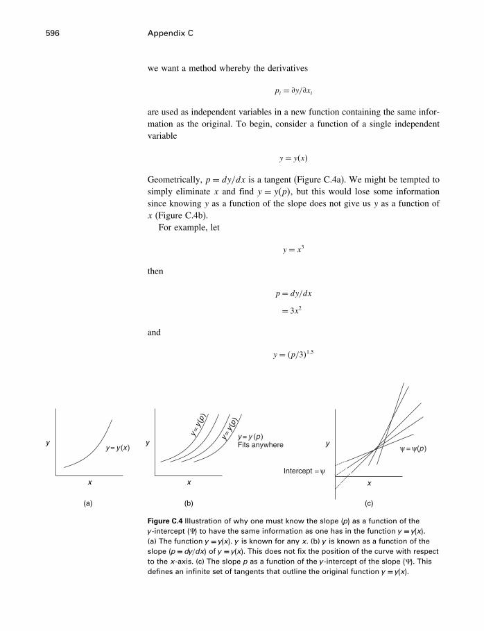
596 Appendix C
we want a method whereby the derivatives
pi = �y/�xi
are used as independent variables in a new function containing the same infor-mation as the original. To begin, consider a function of a single independentvariable
y = y�x�
Geometrically, p= dy/dx is a tangent (Figure C.4a). We might be tempted tosimply eliminate x and find y = y�p�, but this would lose some informationsince knowing y as a function of the slope does not give us y as a function ofx (Figure C.4b).
For example, let
y = x3
then
p= dy/dx= 3x2
and
y = �p/3�1�5
Intercept = ψ
ψ = ψ(p )
(c)
y
x
y = y (x )
(a)
y
x
y = y (p )Fits anywhere
(b)
y
x
y=
y (p
)
y=y (
p )
Figure C.4 Illustration of why one must know the slope �p� as a function of they -intercept ��� to have the same information as one has in the function y = y�x��
(a) The function y = y�x�. y is known for any x� (b) y is known as a function of theslope �p= dy/dx� of y = y�x�. This does not fix the position of the curve with respectto the x-axis. (c) The slope p as a function of the y -intercept of the slope ���. Thisdefines an infinite set of tangents that outline the original function y = y�x��
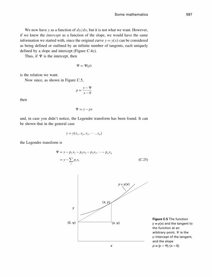
Some mathematics 597
We now have y as a function of dy/dx, but it is not what we want. However,if we knew the intercept as a function of the slope, we would have the sameinformation we started with, since the original curve y= y�x� can be consideredas being defined or outlined by an infinite number of tangents, each uniquelydefined by a slope and intercept (Figure C.4c).
Thus, if is the intercept, then
= �p�
is the relation we want.Now since, as shown in Figure C.5,
p= y− x−0
then
= y−px
and, in case you didn’t notice, the Legendre transform has been found. It canbe shown that in the general case
y = y�x1� x2� x3� · · · � xn�
the Legendre transform is
= y−p1x1−p2x2−p3x3 · · ·−pnxn= y−∑
i
pixi (C.25)
y
x
y = y (x )
(x, y )
(x, ψ)(0, ψ)Figure C.5 The functiony = y�x� and the tangent tothe function at anarbitrary point. � is they -intercept of the tangent,and the slopep= �y −��/�x−0��
598 Appendix C
That is, to form the Legendre transform of a function, subtract from theoriginal function the products of each variable to be changed and the derivativeof the function with respect to that variable. After that, one can proceed to tidyup by eliminating y in the new function by differentiating. Thus in the case ofy = y�x�,
= y−px
d = dy−pdx−xdp=−xdp �dy = pdx by definition�
or
d
dp=−x
and in the general case
d =−∑i
xidpi
For example, if
y = x3
then
p= 3x2
and
= y−x ·3x2
= x3−3x3
=−2x3
or since
x = �p/3� 12
=−2�p/3�32
and
d /dp=−�p/3� 12=−x
Some mathematics 599
Consider another example. If we have
x = y3−3z2
we know x as a function of the two independent variables y and z. If we needa function not of y and z but y and ��x/�z�, we transform one variable, asabove. If we need a function not of y and z or y and ��x/�z� but of ��x/�y�and ��x/�z�, we transform both variables, and invent the new function h, suchthat
h= x−y��x/�y�z− z��x/�z�y
For thermodynamic purposes, that goes far enough, but we can demonstratethat h is a function of ��x/�y� and ��x/�z�. Thus, since
x = y3−3z2
let
p1 = ��x/�y�z= 3y2
and
p2 = ��x/�z�y=−6z
Then
h= y3−3z2−y�3y2�− z�−6z�
=−2y3+3z2
=−2�p1/3�32 +3�−p2/6�2
= �−2/√27�p
321 +p22/12
Thus h is a function of p1 and p2, and
��h/�p1�p2 =−y
and
��h/�p2�p1 =−z
600 Appendix C
Application to thermodynamicsThe Legendre transform is not trivial, but its application to thermodynamicsis. For example, start with U = U�S�V�, which simply says we have a functionU with independent variables S and V . This functional relationship is Equa-tion (4.9), dU = T dS−P dV . Following the recipe, we subtract from U theproduct of each independent variable times the derivative of the function withrespect to that variable. Let’s call the new function G. Thus
G= U −S(�U
�S
)V
−V(�U
�V
)S
and, because ��U/�S�V = T and ��U/�V�S =−P, we get
G= U −TS+PV
It is not easy to see from this definition that G is in fact a function of T andP. To show this, simply write the differential of G,
dG= dU −T dS−S dT +P dV +V dP
and then expand dU by inserting Equation (4.9),
dG= T dS−P dV −T dS−S dT +P dV +V dP=−S dT +V dP (C.26)
From (C.26) we see that the independent variables for G are T and P.By transforming only S we obtain the definition of the Helmholtz energy, and
by transforming only V we get the definition of enthalpy. For more information,see Alberty (2001).
Appendix DHow to use supcrt92
supcrt92 is a FORTRAN program written originally by students and asso-ciates of Prof. H.C. Helgeson at the University of California, Berkeley, andin its present form by J.W. Johnson, Lawrence Livermore National Labora-tory, California. Anyone can use it, free of charge. It uses a large database ofminerals, gases, and aqueous species in which most of the mineral data are fromHelgeson et al. (1978), known as HDNB, which was the first large-scale attemptat obtaining internally consistent data for minerals by including phase equilib-rium data as well as calorimetric and other sources. It uses the Maier–Kelleyheat capacity formulation for minerals, and the revised HKF model foraqueous solutes. It will produce thermodynamic properties to 1000 �C and5000 bars.
The data file is revised periodically by Everett Shock, and available at
http://geopig.asu.edu/supcrt_data.html.
The data file comes in two forms, sequential and direct access. The readablesequential file must be converted into the direct access form that supcrt92uses by using cprons92, a program in the supcrt92 group. Modifications tothe database are made using mprons92. As mentioned in Chapter 13, supcrt92encodes the Haar et al. (1984) equation of state for water, augmented by LeveltSengers et al. (1983) in the critical region. Dielectric constants are derived withthe method of Johnson and Norton (1991).
The program is interactive, with a number of options at each step. Thefollowing instructions are sufficient to get you started, but do not encompassall possibilities. If you get lost, hit Ctrl-C (hold down the Ctrl key and hitletter C), and start again. In the following, program responses which you seeon screen are in italics.
Change to the supcrt92 directory, and type SUPCRT.
Welcome to SUPCRT92 (James W. Johnson, author).last revised 17 July, 1991.would you like to use the default thermodynamic database? (y/n)
601
602 Appendix D
The default database is DPRONS92.DAT, and is out of date. Either renamethe latest version to this, or type “n”, ENTER, enter the name of the databaseyou want to use, then hit ENTER.
choose file option for specifying reaction-independent parameters.1= select one of three default files.2= select an existing nondefault file.3= build a new file.
supcrt92 wants to know what values of T and P you need answers for. Thethree options under no. 1 are often sufficient (see below), and if so, type “1”and hit ENTER. If you want a range of T and P not included in the choicesunder “1” (for example 25 to 1000 �C at 1 and 2 bars), type “3” and hit ENTER.Note that under this option, you also have the choice of having supcrt92 reportthe temperatures of a univariant reaction (logK = 0) at specified pressures,isochoric properties, and other options.
input solvent phase region1= one-phase region.2= liq-vapor saturation curve.3= EQ3/6 one phase/sat grid.
Option 1 gives you a table of answers at every 100 �C from 0 to 1000 �C, atevery pressure from 500 bars to 5000 bars, at 500 bar intervals. Option 2 givesyou answers at 25 �C intervals from 0 to 350 �C along the liquid–vapor curvefor water. Option 3 is for use with programs EQ3 and EQ6. If these options donot suit you, start again and “build a new file” at the previous step. You canspecify a range of T and P, and the intervals.
choose file option for specifying reactions:1= use an existing reaction file.2= build a new reaction file.
You must now specify the reaction (or single mineral, gas, etc.) you areintersted in. If you have done this before, and saved it in a file, choose 1, andthen give the file name when prompted. If this is something new, type “2”, andhit ENTER.
specify number of reactions to be processed.
You can enter up to 50 separate reactions, one after the other. In the fol-lowing, I assume you entered “1”.
input title for reaction 1 of 1.
This title will appear on the output for convenience. It does not affect thecalculations.
How to use supcrt92 603
enter [coeff species] pairs, separated by blanks, one pair per line, for reaction1 (conclude with [0 done]).
Enter the desired reaction with each stoichiometric coefficient and species,separated by a blank, on a separate line. Use negative coefficients for reactantsand positive coefficients for products. supcrt92 does not check if the reactionis balanced, or if it makes any sense. Each species must be written exactly asit appears in the database, because supcrt92 uses the name to find the data.Minerals must be typed in capital letters, aqueous species in capitals, lowercase, numerals, and + or − as indicated, and so on.
For example, the reaction
Ca3Fe2Si3O12+4H2S�aq�+2Cu++3CO2�g�
= 3SiO2�qtz�+3CaCO3+2CuFeS2+2H++3H2O
would be entered as follows:−1 ANDRADITE−4 H2S,aq−2 Cu+−3 CO2,g3 QUARTZ3 CALCITE2 CHALCOPYRITE2 H+3 H2O0
You don’t need to type “done”.Note that if you want the properties of a single mineral, ion, or gas, just enter
that mineral or ion as a product, with no reactants. For example, for tables ofthe thermodynamic properties of halite (including �aG
� and �aH�), just enter1 HALITE0
reaction 1 stoichiometry. Is this correct?
The program repeats your input. If you made an error, type “n”, and repeat.If the program detects an error (a mineral misspelled, or not in the database) itwill tell you, and you need only repeat that entry.
would you like to save these reactions to a file (y/n)
If you will be using this reaction repeatedly, type “y”. You can then use thisfile at the earlier prompt, choose file option for specifying reactions.
specify name for tabulated output file:
This is the name of the file your results will be in.
604 Appendix D
would you like to generate x-y plot files for logK, G, H, S, Cp, and V ofreaction? (y/n)
If you say “y”, you get a whole bunch of files with your data arranged in away more convenient for plotting. The format is such that with minimal editingthey can be read and used by spreadsheets and plotting programs. You get allor none of them. They have extensions .kxy, .gxy, .hxy, and so on.
reaction in progress…
…a few more messages…
…execution completedYour results should now be in the file with the name you specified.
Appendix EComputer programs
E.1 Fortran
The Pitzer equations have quite a formidable appearance, and although Harvieand Weare (1980) claim that implementation is “rather simple,” it can be quitea chore, especially if many components and potential solids are considered. Theequations have many double summation terms, and it can be hard to visualizewhat they would look like when implemented. To help readers understandthese equations, I have written a FORTRAN program to calculate the solubilityof gypsum in mixed NaCl–Na2SO4 solutions at 25 �C. Shown here are twosubroutines, which implement the Pitzer approach for this system. The completeprogram contains additional subroutines which solve for the gypsum contentand test whether the solubility product is satisfied, but they have nothing todo with the Pitzer model, and are not included here. The program can bedownloaded from http://www.cambridge.org/0521847729. If you do have tocopy it, omit the line numbers.
E.1.1 Subroutine Pitzer
Given the concentrations of Na, Ca, Cl, and SO4 (as some combination of NaCland Na2SO4), this subroutine calculates the activity coefficients of Ca and SO4
and the activity of water, using the Pitzer equations and the parameters fromHarvie and Weare (1980). The expression aCa2+aSO2−
4a2H2O
can then be testedagainst the solubility product.
Even readers not familiar with FORTRAN should be able to see how themany summation signs in the Pitzer equations are expanded into actual expres-sions, and how the many parameters fit in. The equations are broken up intoterm1, term2, etc., to correspond with the text in §15.7.2. Here are somecomments which may help to understand the program.
• Statements beginning with ! are comments, and are ignored by the program. Symbol
& indicates that the statement is continued on the next line.• Many computer languages, includingFORTRAN, require that every variable be initially
declared as to its type,whether character, real number, integer, logical, etc.Lines9–29do
605
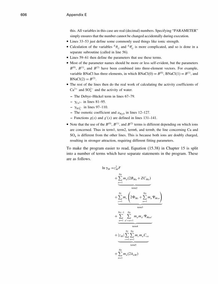
606 Appendix E
this. All variables in this case are real (decimal) numbers. Specifying “PARAMETER”
simply ensures that the number cannot be changed accidentally during execution.• Lines 33–53 just define some commonly used things like ionic strength.• Calculation of the variables E�ij and
E�′ij is more complicated, and so is done in a
separate subroutine (called in line 56).• Lines 59–61 then define the parameters that use these terms.• Most of the parameter names should be more or less self-evident, but the parameters
B�0�, B�1�, and B�2� have been combined into three-element vectors. For example,
variable BNaCl has three elements, in which BNaCl�0�= B�0�, BNaCl�1�= B�1�, andBNaCl�2�= B�2�.
• The rest of the lines then do the real work of calculating the activity coefficients of
Ca2+ and SO2−4 and the activity of water.
– The Debye–Hückel term in lines 67–79.
– Ca2+ in lines 81–95.
– SO2−4
in lines 97–110.
– The osmotic coefficient and aH2Oin lines 12–127.
– Functions g�x� and g′�x� are defined in lines 131–141.
• Note that the use of the B�0�, B�1�, and B�2� terms is different depending on which ions
are concerned. Thus in term1, term2, term6, and termb, the line concerning Ca and
SO4 is different from the other lines. This is because both ions are doubly charged,
resulting in stronger attraction, requiring different fitting parameters.
To make the program easier to read, Equation (15.38) in Chapter 15 is splitinto a number of terms which have separate statements in the program. Theseare as follows.
lnM =z2MF
+Na∑a=1
ma�2BMa+ZCMa�︸ ︷︷ ︸term2
+Nc∑c=1
mc
(2�Mc+
Na∑a=1
ma Mca
)︸ ︷︷ ︸
term3
+Na−1∑a=1
Na∑a′=a+1
mama′ Maa′︸ ︷︷ ︸term4
+�zM �Nc∑c=1
Na∑a=1
mcmaCca︸ ︷︷ ︸term5
+Nn∑n=1
mn�2�nM�
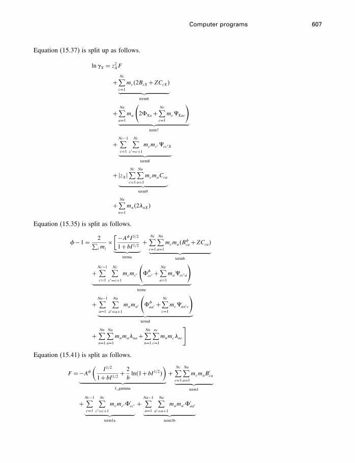
Computer programs 607
Equation (15.37) is split up as follows.
lnX = z2XF
+Nc∑c=1
mc�2BcX+ZCcX�︸ ︷︷ ︸term6
+Na∑a=1
ma
(2�Xa+
Nc∑c=1
mc Xac
)︸ ︷︷ ︸
term7
+Nc−1∑c=1
Nc∑c′=c+1
mcmc′ cc′X︸ ︷︷ ︸term8
+�zX�Nc∑c=1
Na∑a=1
mcmaCca︸ ︷︷ ︸term9
+Nn∑n=1
mn�2�nX�
Equation (15.35) is split as follows.
�−1= 2∑i mi
×[−A�I3/21+bI1/2︸ ︷︷ ︸
terma
+Nc∑c=1
Na∑a=1
mcma�B�ca+ZCca�︸ ︷︷ ︸
termb
+Nc−1∑c=1
Nc∑c′=c+1
mcmc′
(��cc′ +
Na∑a=1
ma cc′a
)︸ ︷︷ ︸
termc
+Na−1∑a=1
Na∑a′=a+1
mama′
(��aa′ +
Nc∑c=1
mc aa′c
)︸ ︷︷ ︸
termd
+Nn∑n=1
Na∑a=1
mnma�na+Nn∑n=1
nc∑c=1
mnmc�nc
]
Equation (15.41) is split as follows.
F =−A�(
I1/2
1+bI1/2 +2bln�1+bI1/2�
)︸ ︷︷ ︸
f_gamma
+Nc∑c=1
Na∑a=1
mcmaB′ca︸ ︷︷ ︸
term1
+Nc−1∑c=1
Nc∑c′=c+1
mcmc′�′cc′︸ ︷︷ ︸
term1a
+Na−1∑a=1
Na∑a′=a+1
mama′�′aa′︸ ︷︷ ︸
term1b
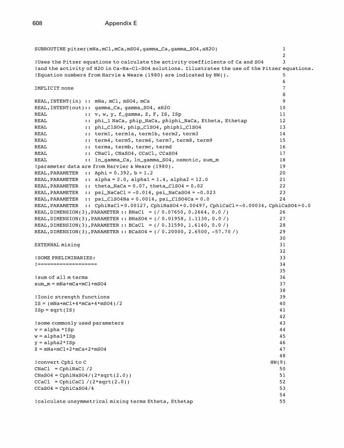
608 Appendix E
SUBROUTINE pitzer(mNa,mCl,mCa,mSO4,gamma_Ca,gamma_SO4,aH2O) 12
!Uses the Pitzer equations to calculate the activity coefficients of Ca and SO4 3!and the activity of H2O in Ca-Na-Cl-SO4 solutions. Illustrates the use of the Pitzer equations.!Equation numbers from Harvie & Weare (1980) are indicated by HW(). 5
6IMPLICIT none 7
8REAL,INTENT(in) :: mNa, mCl, mSO4, mCa 9REAL,INTENT(out):: gamma_Ca, gamma_SO4, aH2O 10REAL :: v, w, y, f_gamma, Z, F, IS, ISp 11REAL :: phi_1 NaCa, phip_NaCa, phiphi_NaCa, Etheta, Ethetap 12REAL :: phi_ClSO4, phip_ClSO4, phiphi_ClSO4 13REAL :: term1, term1a, term1b, term2, term3 14REAL :: term4, term5, term6, term7, term8, term9 15REAL :: terma, termb, termc, termd 16REAL :: CNaCl, CNaSO4, CCaCl, CCaSO4 17REAL :: ln_gamma_Ca, ln_gamma_SO4, osmotic, sum_m 18!parameter data are from Harvier & Weare (1980). 19REAL,PARAMETER :: Aphi = 0.392, b = 1.2 20REAL,PARAMETER :: alpha = 2.0, alpha1 = 1.4, alpha2 = 12.0 21REAL,PARAMETER :: theta_NaCa = 0.07, theta_ClSO4 = 0.02 22REAL,PARAMETER :: psi_NaCaCl = -0.014, psi_NaCaSO4 = -0.023 23REAL,PARAMETER :: psi_ClSO4Na = 0.0014, psi_ClSO4Ca = 0.0 24REAL,PARAMETER :: CphiNaCl=0.00127, CphiNaSO4=0.00497, CphiCaCl=-0.00034, CphiCaSO4=0.0REAL,DIMENSION(3),PARAMETER :: BNaCl = (/ 0.07650, 0.2664, 0.0 /) 26REAL,DIMENSION(3),PARAMETER :: BNaSO4 = (/ 0.01958, 1.1130, 0.0 /) 27REAL,DIMENSION(3),PARAMETER :: BCaCl = (/ 0.31590, 1.6140, 0.0 /) 28REAL,DIMENSION(3),PARAMETER :: BCaSO4 = (/ 0.20000, 2.6500, -57.70 /) 29
30EXTERNAL mixing 31
32!SOME PRELIMINARIES: 33!=================== 34
35!sum of all m terms 36sum_m = mNa+mCa+mCl+mSO4 37
38!Ionic strength functions 39IS = (mNa+mCl+4*mCa+4*mSO4)/2 40ISp = sqrt(IS) 41
42!some commonly used parameters 43v = alpha *ISp 44w = alpha1*ISp 45y = alpha2*ISp 46Z = mNa+mCl+2*mCa+2*mSO4 47
48!convert Cphi to C HW(9)CNaCl = CphiNaCl /2 50CNaSO4 = CphiNaSO4/(2*sqrt(2.0)) 51CCaCl = CphiCaCl /(2*sqrt(2.0)) 52CCaSO4 = CphiCaSO4/4 53
54!calculate unsymmetrical mixing terms Etheta, Ethetap 55
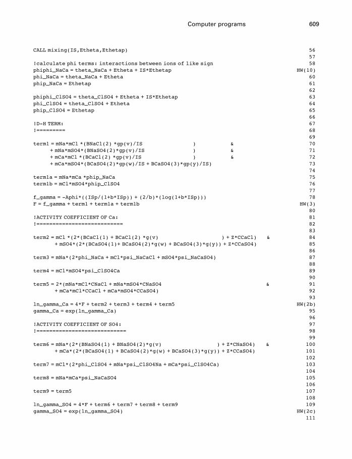
Computer programs 609
CALL mixing(IS,Etheta,Ethetap) 5657
!calculate phi terms: interactions between ions of like sign 58phiphi_NaCa = theta_NaCa + Etheta + IS*Ethetap HW(10)phi_NaCa = theta_NaCa + Etheta 60phip_NaCa = Ethetap 61
62phiphi_ClSO4 = theta_ClSO4 + Etheta + IS*Ethetap 63phi_ClSO4 = theta_ClSO4 + Etheta 64phip_ClSO4 = Ethetap 65
66!D-H TERM: 67!========= 68
69term1 = mNa*mCl *(BNaCl(2) *gp(v)/IS ) & 70
+ mNa*mSO4*(BNaSO4(2)*gp(v)/IS ) & 71+ mCa*mCl *(BCaCl(2) *gp(v)/IS ) & 72+ mCa*mSO4*(BCaSO4(2)*gp(w)/IS + BCaSO4(3)*gp(y)/IS) 73
74term1a = mNa*mCa *phip_NaCa 75term1b = mCl*mSO4*phip_ClSO4 76
77f_gamma = -Aphi*((ISp/(1+b*ISp)) + (2/b)*(log(1+b*ISp))) 78F = f_gamma + term1 + term1a + term1b HW(3)
80!ACTIVITY COEFFICIENT OF Ca: 81!=========================== 82
83term2 = mCl *(2*(BCaCl(1) + BCaCl(2) *g(v) ) + Z*CCaCl) & 84
+ mSO4*(2*(BCaSO4(1)+ BCaSO4(2)*g(w) + BCaSO4(3)*g(y)) + Z*CCaSO4) 8586
term3 = mNa*(2*phi_NaCa + mCl*psi_NaCaCl + mSO4*psi_NaCaSO4) 8788
term4 = mCl*mSO4*psi_ClSO4Ca 8990
term5 = 2*(mNa*mCl*CNaCl + mNa*mSO4*CNaSO4 & 91+ mCa*mCl*CCaCl + mCa*mSO4*CCaSO4) 92
93ln_gamma_Ca = 4*F + term2 + term3 + term4 + term5 HW(2b)gamma_Ca = exp(ln_gamma_Ca) 95
96!ACTIVITY COEFFICIENT OF SO4: 97!============================ 98
99term6 = mNa*(2*(BNaSO4(1) + BNaSO4(2)*g(v) ) + Z*CNaSO4) & 100
+ mCa*(2*(BCaSO4(1) + BCaSO4(2)*g(w) + BCaSO4(3)*g(y)) + Z*CCaSO4) 101102
term7 = mCl*(2*phi_ClSO4 + mNa*psi_ClSO4Na + mCa*psi_ClSO4Ca) 103104
term8 = mNa*mCa*psi_NaCaSO4 105106
term9 = term5 107108
ln_gamma_SO4 = 4*F + term6 + term7 + term8 + term9 109gamma_SO4 = exp(ln_gamma_SO4) HW(2c)
111
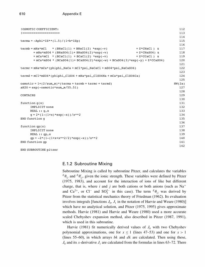
610 Appendix E
!OSMOTIC COEFFICIENT: 112!==================== 113
114terma = -Aphi*IS**(1.5)/(1+b*ISp) 115
116termb = mNa*mCl * (BNaCl(1) + BNaCl(2) *exp(-v) + Z*CNaCl ) & 117
+ mNa*mSO4 * (BNaSO4(1)+ BNaSO4(2)*exp(-v) + Z*CNaSO4) & 118+ mCa*mCl * (BCaCl(1) + BCaCl(2) *exp(-v) + Z*CCaCl ) & 119+ mCa*mSO4 * (BCaSO4(1)+ BCaSO4(2)*exp(-w) + BCaSO4(3)*exp(-y) + Z*CCaSO4) 120
121termc = mNa*mCa*(phiphi_NaCa + mCl*psi_NaCaCl + mSO4*psi_NaCaSO4) 122
123termd = mCl*mSO4*(phiphi_ClSO4 + mNa*psi_ClSO4Na + mCa*psi_ClSO4Ca) 124
125osmotic = 1+(2/sum_m)*(terma + termb + termc + termd) HW(2a)aH2O = exp(-osmotic*sum_m/55.51) 127
128CONTAINS 129
130function g(x) 131
IMPLICIT none 132REAL :: g,x 133g = 2*(1-(1+x)*exp(-x))/x**2 134
END function g 135136
function gp(x) 137IMPLICIT none 138REAL :: gp,x 139gp = -2*(1-(1+x+x**2/2)*exp(-x))/x**2 140
END function gp 141142
END SUBROUTINE pitzer
E.1.2 Subroutine Mixing
Subroutine Mixing is called by subroutine Pitzer, and calculates the variablesE�ij and
E�′ij , given the ionic strength. These variables were defined by Pitzer(1975, 1983), and account for the interaction of ions of like but differentcharge, that is, where i and j are both cations or both anions (such as Na+
and Ca2+, or Cl− and SO2−4 in this case). The term E�ij was derived by
Pitzer from the statistical mechanics theory of Friedman (1962). Its evaluationinvolves integrals [functions J0, J1 in the notation of Harvie and Weare (1980)]which have no analytical solution, and Pitzer (1975, 1995) gives approximatemethods. Harvie (1981) and Harvie and Weare (1980) used a more accuratescaled Chebyshev expansion method, also described in Pitzer (1987, 1991),which is used in this subroutine.
Harvie (1981) fit numerically derived values of J0 with two Chebyshevpolynomial approximations, one for x ≤ 1 (lines 47–53) and one for x > 1(lines 55–60), in which arrays bk and dk are calculated. Then using these,J0 and its x-derivative J1 are calculated from the formulas in lines 63–72. There
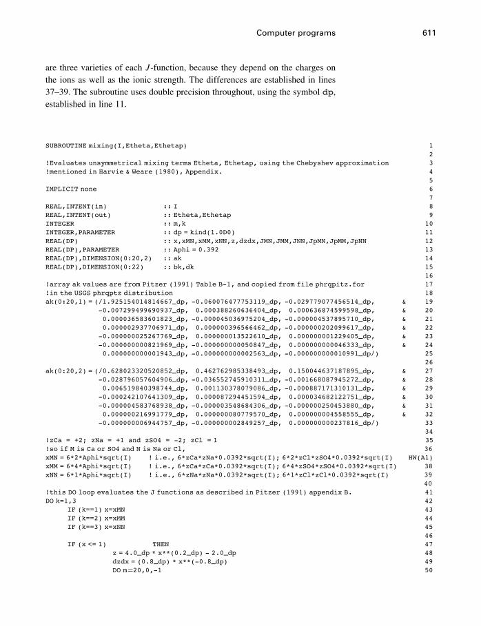
Computer programs 611
are three varieties of each J -function, because they depend on the charges onthe ions as well as the ionic strength. The differences are established in lines37–39. The subroutine uses double precision throughout, using the symbol dp,established in line 11.
SUBROUTINE mixing(I,Etheta,Ethetap) 12
!Evaluates unsymmetrical mixing terms Etheta, Ethetap, using the Chebyshev approximation 3!mentioned in Harvie & Weare (1980), Appendix. 4
5IMPLICIT none 6
7REAL,INTENT(in) :: I 8REAL,INTENT(out) :: Etheta,Ethetap 9INTEGER :: m,k 10INTEGER,PARAMETER :: dp = kind(1.0D0) 11REAL(DP) :: x,xMN,xMM,xNN,z,dzdx,JMN,JMM,JNN,JpMN,JpMM,JpNN 12REAL(DP),PARAMETER :: Aphi = 0.392 13REAL(DP),DIMENSION(0:20,2) :: ak 14REAL(DP),DIMENSION(0:22) :: bk,dk 15
16!array ak values are from Pitzer (1991) Table B-1, and copied from file phrqpitz.for 17!in the USGS phrqptz distribution 18ak(0:20,1) = (/1.925154014814667_dp, -0.060076477753119_dp, -0.029779077456514_dp, & 19
-0.007299499690937_dp, 0.000388260636404_dp, 0.000636874599598_dp, & 200.000036583601823_dp, -0.000045036975204_dp, -0.000004537895710_dp, & 210.000002937706971_dp, 0.000000396566462_dp, -0.000000202099617_dp, & 22
-0.000000025267769_dp, 0.000000013522610_dp, 0.000000001229405_dp, & 23-0.000000000821969_dp, -0.000000000050847_dp, 0.000000000046333_dp, & 240.000000000001943_dp, -0.000000000002563_dp, -0.000000000010991_dp/) 25
26ak(0:20,2) = (/0.628023320520852_dp, 0.462762985338493_dp, 0.150044637187895_dp, & 27
-0.028796057604906_dp, -0.036552745910311_dp, -0.001668087945272_dp, & 280.006519840398744_dp, 0.001130378079086_dp, -0.000887171310131_dp, & 29
-0.000242107641309_dp, 0.000087294451594_dp, 0.000034682122751_dp, & 30-0.000004583768938_dp, -0.000003548684306_dp, -0.000000250453880_dp, & 310.000000216991779_dp, 0.000000080779570_dp, 0.000000004558555_dp, & 32
-0.000000006944757_dp, -0.000000002849257_dp, 0.000000000237816_dp/) 3334
!zCa = +2; zNa = +1 and zSO4 = -2; zCl = 1 35!so if M is Ca or SO4 and N is Na or Cl, 36xMN = 6*2*Aphi*sqrt(I) ! i.e., 6*zCa*zNa*0.0392*sqrt(I); 6*2*zCl*zSO4*0.0392*sqrt(I) HW(A1)xMM = 6*4*Aphi*sqrt(I) ! i.e., 6*zCa*zCa*0.0392*sqrt(I); 6*4*zSO4*zSO4*0.0392*sqrt(I) 38xNN = 6*1*Aphi*sqrt(I) ! i.e., 6*zNa*zNa*0.0392*sqrt(I); 6*1*zCl*zCl*0.0392*sqrt(I) 39
40!this DO loop evaluates the J functions as described in Pitzer (1991) appendix B. 41DO k=1,3 42
IF (k==1) x=xMN 43IF (k==2) x=xMM 44IF (k==3) x=xNN 45
46IF (x <= 1) THEN 47
z = 4.0_dp * x**(0.2_dp) - 2.0_dp 48dzdx = (0.8_dp) * x**(-0.8_dp) 49DO m=20,0,-1 50
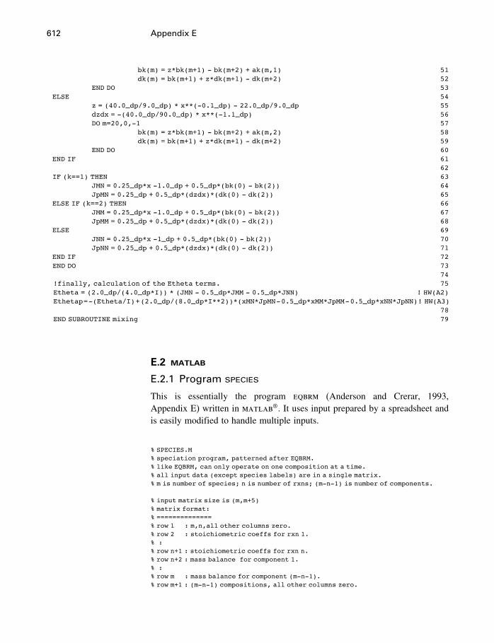
612 Appendix E
bk(m) = z*bk(m+1) - bk(m+2) + ak(m,1) 51dk(m) = bk(m+1) + z*dk(m+1) - dk(m+2) 52
END DO 53ELSE 54
z = (40.0_dp/9.0_dp) * x**(-0.1_dp) - 22.0_dp/9.0_dp 55dzdx = -(40.0_dp/90.0_dp) * x**(-1.1_dp) 56DO m=20,0,-1 57
bk(m) = z*bk(m+1) - bk(m+2) + ak(m,2) 58dk(m) = bk(m+1) + z*dk(m+1) - dk(m+2) 59
END DO 60END IF 61
62IF (k==1) THEN 63
JMN = 0.25_dp*x -1.0_dp + 0.5_dp*(bk(0) - bk(2)) 64JpMN = 0.25_dp + 0.5_dp*(dzdx)*(dk(0) - dk(2)) 65
ELSE IF (k==2) THEN 66JMM = 0.25_dp*x -1.0_dp + 0.5_dp*(bk(0) - bk(2)) 67JpMM = 0.25_dp + 0.5_dp*(dzdx)*(dk(0) - dk(2)) 68
ELSE 69JNN = 0.25_dp*x -1_dp + 0.5_dp*(bk(0) - bk(2)) 70JpNN = 0.25_dp + 0.5_dp*(dzdx)*(dk(0) - dk(2)) 71
END IF 72END DO 73
74!finally, calculation of the Etheta terms. 75Etheta = (2.0_dp/(4.0_dp*I)) * (JMN - 0.5_dp*JMM - 0.5_dp*JNN) ! HW(A2)Ethetap=-(Etheta/I)+(2.0_dp/(8.0_dp*I**2))*(xMN*JpMN-0.5_dp*xMM*JpMM-0.5_dp*xNN*JpNN)! HW(A3)
78END SUBROUTINE mixing 79
E.2 matlab
E.2.1 Program species
This is essentially the program eqbrm (Anderson and Crerar, 1993,Appendix E) written in matlab®. It uses input prepared by a spreadsheet andis easily modified to handle multiple inputs.
% SPECIES.M% speciation program, patterned after EQBRM.% like EQBRM, can only operate on one composition at a time.% all input data (except species labels) are in a single matrix.% m is number of species; n is number of rxns; (m-n-1) is number of components.
% input matrix size is (m,m+5)% matrix format:% ==============% row 1 : m,n,all other columns zero.% row 2 : stoichiometric coeffs for rxn 1.% :% row n+1 : stoichiometric coeffs for rxn n.% row n+2 : mass balance for component 1.% :% row m : mass balance for component (m-n-1).% row m+1 : (m-n-1) compositions, all other columns zero.
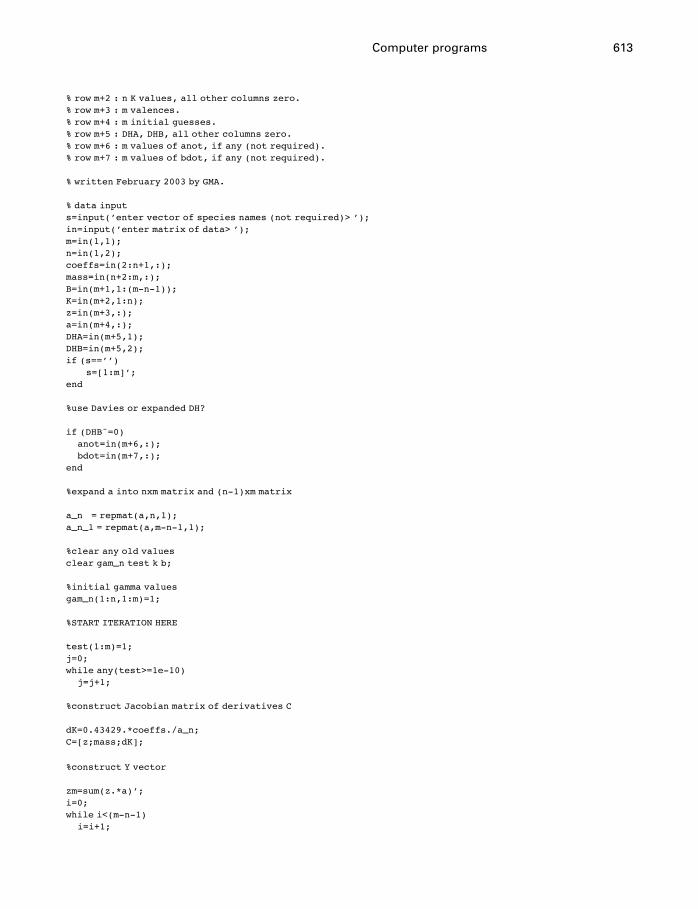
Computer programs 613
% row m+2 : n K values, all other columns zero.% row m+3 : m valences.% row m+4 : m initial guesses.% row m+5 : DHA, DHB, all other columns zero.% row m+6 : m values of anot, if any (not required).% row m+7 : m values of bdot, if any (not required).
% written February 2003 by GMA.
% data inputs=input(’enter vector of species names (not required)> ’);in=input(’enter matrix of data> ’);m=in(1,1);n=in(1,2);coeffs=in(2:n+1,:);mass=in(n+2:m,:);B=in(m+1,1:(m-n-1));K=in(m+2,1:n);z=in(m+3,:);a=in(m+4,:);DHA=in(m+5,1);DHB=in(m+5,2);if (s==’’)
s=[1:m]’;end
%use Davies or expanded DH?
if (DHB˜=0)anot=in(m+6,:);bdot=in(m+7,:);
end
%expand a into nxm matrix and (n-1)xm matrix
a_n = repmat(a,n,1);a_n_1 = repmat(a,m-n-1,1);
%clear any old valuesclear gam_n test k b;
%initial gamma valuesgam_n(1:n,1:m)=1;
%START ITERATION HERE
test(1:m)=1;j=0;while any(test>=1e-10)
j=j+1;
%construct Jacobian matrix of derivatives C
dK=0.43429.*coeffs./a_n;C=[z;mass;dK];
%construct Y vector
zm=sum(z.*a)’;i=0;while i<(m-n-1)
i=i+1;
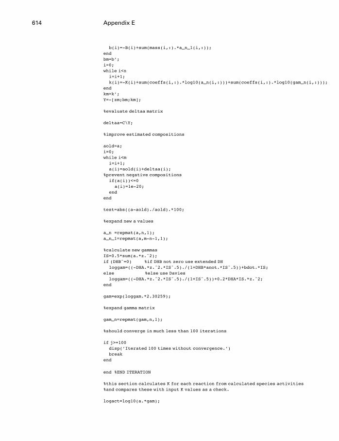
614 Appendix E
b(i)=-B(i)+sum(mass(i,:).*a_n_1(i,:));endbm=b’;i=0;while i<n
i=i+1;k(i)=-K(i)+sum(coeffs(i,:).*log10(a_n(i,:)))+sum(coeffs(i,:).*log10(gam_n(i,:)));
endkm=k’;Y=-[zm;bm;km];
%evaluate deltaa matrix
deltaa=C\Y;
%improve estimated compositions
aold=a;i=0;while i<m
i=i+1;a(i)=aold(i)+deltaa(i);
%prevent negative compositionsif(a(i))<=0
a(i)=1e-20;end
end
test=abs((a-aold)./aold).*100;
%expand new a values
a_n =repmat(a,n,1);a_n_1=repmat(a,m-n-1,1);
%calculate new gammasIS=0.5*sum(a.*z.ˆ2);if (DHB˜=0) %if DHB not zero use extended DH
loggam=((-DHA.*z.ˆ2.*ISˆ.5)./(1+DHB*anot.*ISˆ.5))+bdot.*IS;else %else use Davies
loggam=((-DHA.*z.ˆ2.*ISˆ.5)./(1+ISˆ.5))+0.2*DHA*IS.*z.ˆ2;end
gam=exp(loggam.*2.30259);
%expand gamma matrix
gam_n=repmat(gam,n,1);
%should converge in much less than 100 iterations
if j>=100disp(’Iterated 100 times without convergence.’)break
end
end %END ITERATION
%this section calculates K for each reaction from calculated species activities%and compares these with input K values as a check.
logact=log10(a.*gam);
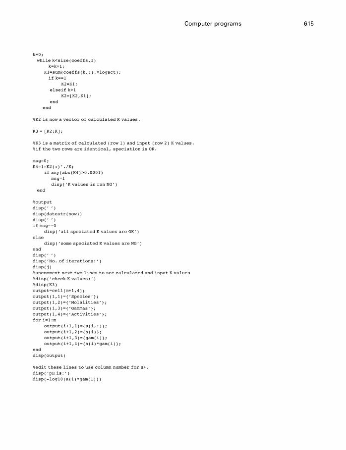
Computer programs 615
k=0;while k<size(coeffs,1)
k=k+1;K1=sum(coeffs(k,:).*logact);if k==1
K2=K1;elseif k>1
K2=[K2,K1];end
end
%K2 is now a vector of calculated K values.
K3 = [K2;K];
%K3 is a matrix of calculated (row 1) and input (row 2) K values.%if the two rows are identical, speciation is OK.
msg=0;K4=1-K2(:)’./K;
if any(abs(K4)>0.0001)msg=1disp(’K values in rxn NG’)
end
%outputdisp(’ ’)disp(datestr(now))disp(’ ’)if msg==0
disp(’all speciated K values are OK’)else
disp(’some speciated K values are NG’)enddisp(’ ’)disp(’No. of iterations:’)disp(j)%uncomment next two lines to see calculated and input K values%disp(’check K values:’)%disp(K3)output=cell(m+1,4);output(1,1)={’Species’};output(1,2)={’Molalities’};output(1,3)={’Gammas’};output(1,4)={’Activities’};for i=1:m
output(i+1,1)={s(i,:)};output(i+1,2)={a(i)};output(i+1,3)={gam(i)};output(i+1,4)={a(i)*gam(i)};
enddisp(output)
%edit these lines to use column number for H+.disp(’pH is:’)disp(-log10(a(1)*gam(1)))
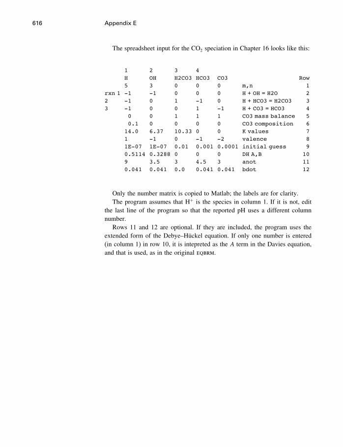
616 Appendix E
The spreadsheet input for the CO2 speciation in Chapter 16 looks like this:
1 2 3 4H OH H2CO3 HCO3 CO3 Row5 3 0 0 0 m,n 1
rxn 1 -1 -1 0 0 0 H + OH = H2O 22 -1 0 1 -1 0 H + HCO3 = H2CO3 33 -1 0 0 1 -1 H + CO3 = HCO3 4
0 0 1 1 1 CO3 mass balance 50.1 0 0 0 0 CO3 composition 6
14.0 6.37 10.33 0 0 K values 71 -1 0 -1 -2 valence 81E-07 1E-07 0.01 0.001 0.0001 initial guess 90.5114 0.3288 0 0 0 DH A,B 109 3.5 3 4.5 3 anot 110.041 0.041 0.0 0.041 0.041 bdot 12
Only the number matrix is copied to Matlab; the labels are for clarity.The program assumes that H+ is the species in column 1. If it is not, edit
the last line of the program so that the reported pH uses a different columnnumber.
Rows 11 and 12 are optional. If they are included, the program uses theextended form of the Debye–Hückel equation. If only one number is entered(in column 1) in row 10, it is intepreted as the A term in the Davies equation,and that is used, as in the original eqbrm.
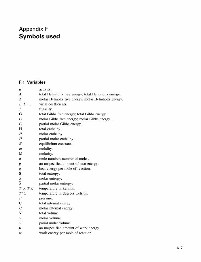
Appendix FSymbols used
F.1 Variables
a activity.A total Helmholtz free energy; total Helmholtz energy.A molar Helmoltz free energy, molar Helmholtz energy.B, C,… virial coefficients.f fugacity.G total Gibbs free energy; total Gibbs energy.G molar Gibbs free energy; molar Gibbs energy.G partial molar Gibbs energy.H total enthalpy.H molar enthalpy.H partial molar enthalpy.K equilibrium constant.m molality.M molarity.n mole number; number of moles.q an unspecified amount of heat energy.q heat energy per mole of reaction.S total entropy.S molar entropy.S partial molar entropy.T or T K temperature in kelvins.T �C temperature in degrees Celsius.P pressure.U total internal energy.U molar internal energy.V total volume.V molar volume.V parial molar volume.w an unspecified amount of work energy.w work energy per mole of reaction.
617
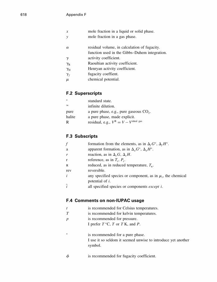
618 Appendix F
x mole fraction in a liquid or solid phase.y mole fraction in a gas phase.
residual volume, in calculation of fugacity.function used in the Gibbs–Duhem integration.
activity coefficient.R Raoultian activity coefficient.H Henryan activity coefficient.f fugacity coeffient.� chemical potential.
F.2 Superscripts� standard state.� infinite dilution.pure a pure phase, e.g., pure gaseous CO2.halite a pure phase, made explicit.R residual, e.g., V R = V −V ideal gas
F.3 Subscripts
f formation from the elements, as in �fG�, �fH
�.a apparent formation, as in �aG
�, �aH�.r reaction, as in �rG, �rH .r reference, as in Tr , Pr .r reduced, as in reduced temperature, Tr.rev reversible.i any specified species or component, as in �i, the chemical
potential of i.i all specified species or components except i.
F.4 Comments on non-IUPAC usage
t is recommended for Celsius temperatures.T is recommended for kelvin temperatures.p is recommended for pressure.
I prefer T �C, T or T K, and P.
∗ is recommended for a pure phase.I use it so seldom it seemed unwise to introduce yet anothersymbol.
� is recommended for fugacity coefficient.
Symbols used 619
f is recommended for Raoultian activity coefficient.
m is recommended for Henryan activity coefficient, usingmolalities.I prefer f , R, and H to indicate the essential similarity ofthese quantities.
V , H , etc. is assumed for total volume, total enthalpy, etc.Vm, Hm, etc. is recommended for molar volume, molar enthalpy, etc.
although lower case v, h, etc., is becoming common too.V ′, H ′, etc. is recommended for partial molar quantities.
The distinction between total and molar quantities is of coursevital to understanding thermodynamics. I prefer to emphasize thisdifference by using bold symbols for total quantities, as shownabove. I have previously used roman and italic letters (e.g., Vversus V ) for this distinction, but now believe this is an insuffi-cient distinction. The overbar notation for partial molar quantities(e.g., V ) is widely used, and I prefer it.
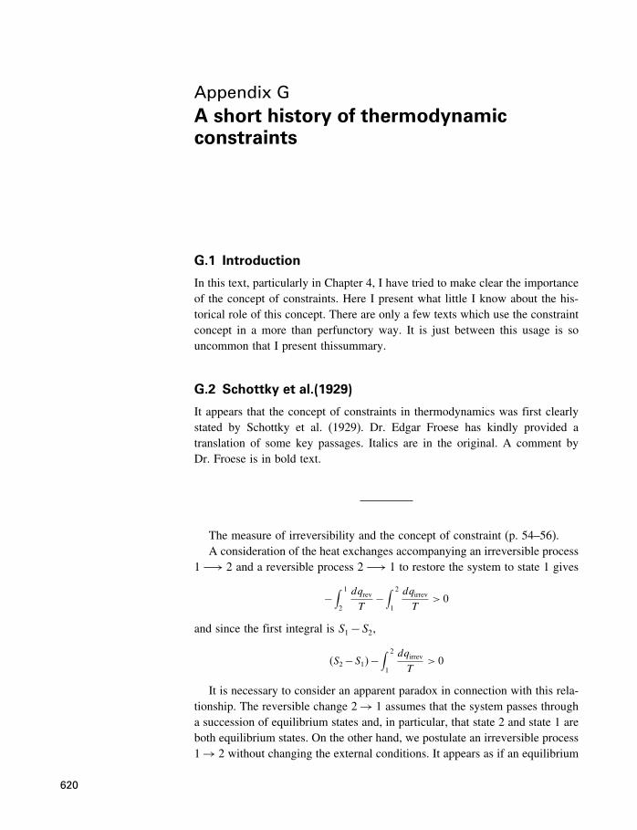
Appendix GA short history of thermodynamicconstraints
G.1 Introduction
In this text, particularly in Chapter 4, I have tried to make clear the importanceof the concept of constraints. Here I present what little I know about the his-torical role of this concept. There are only a few texts which use the constraintconcept in a more than perfunctory way. It is just between this usage is souncommon that I present thissummary.
G.2 Schottky et al.(1929)
It appears that the concept of constraints in thermodynamics was first clearlystated by Schottky et al. (1929). Dr. Edgar Froese has kindly provided atranslation of some key passages. Italics are in the original. A comment byDr. Froese is in bold text.
The measure of irreversibility and the concept of constraint (p. 54–56).A consideration of the heat exchanges accompanying an irreversible process
1−→ 2 and a reversible process 2−→ 1 to restore the system to state 1 gives
−∫ 1
2
dqrevT
−∫ 2
1
dqirrevT
> 0
and since the first integral is S1−S2,
�S2−S1�−∫ 2
1
dqirrevT
> 0
It is necessary to consider an apparent paradox in connection with this rela-tionship. The reversible change 2→ 1 assumes that the system passes througha succession of equilibrium states and, in particular, that state 2 and state 1 areboth equilibrium states. On the other hand, we postulate an irreversible process1→ 2 without changing the external conditions. It appears as if an equilibrium
620
A short history of thermodynamic constraints 621
state changed spontaneously to a different state. Thus it appears not to havebeen in equilibrium.
The solution to this paradox, which, in fact, is necessary to make the previousdeductions valid, is that state 1 is a constrained system. It does not proceedirreversibly to state 2 because it is hindered to do so by some constraints. Werethese constraints absolute, never to be released, the previous considerationswould have been pointless; the application is rather limited to constraints whichcan be arbitrarily removed (without thermodynamic means) thus permitting theirreversible process 1→ 2. Such constraints can be, e.g. produced by:
• locking a piston in a cylinder separating two gases at different pressures;
• resistance to deformation of a solid;
• constraints in chemical change like nonreacting cold H2 and O2;
• constraints in heat exchange between different parts of a system.
In all these cases, a further condition must be fulfilled in order to assign adefinite entropy increase to the irreversible changes. It must be possible notonly to release the constraints and thereby induce the change to state 2, butalso, after the release of the constraints and after completion of the process,to bring about a reversible restoration of the change by means of only exter-nal thermodynamic effects. After all, only in such case is a thermodynamicdefinition and determination of entropy possible.
The independent chemical changes as constrained changes (p. 135; p. 144)Changes here considered are characterized by the fact that they can occur
at fixed external conditions. Therefore, they are constrained changes. We aredealing with different equilibrium states at the same physical conditions (sametemperature and either same P or V ). That is only possible if these are con-straints to the progress of these considered changes. Example: the reaction2H2+O2 → 2H2O, at ordinary temperatures, is generally a constrained reac-tion. A catalyst or heating will cause the system to leave its apparently, stableequilibrium state. We can say, generally, that chemical thermodynamics isthermodynamics of constrained equilibrium states. There is only one state of asystem which will not change upon removal of the constraint; that is the stateof complete, unconstrained equilibrium.
The multiplicity of the inner (chemical) state, which is independent of exter-nal conditions, is made possible only by the fact that the transition of innerstates, from one to another, is a constrained process.
Schottky et al. (1929) proceeded to derive the extent of reaction �
(p. 151), apparently independently of De Donder (1920). There is no definitestatement that � is used as a possible constraint, but I think it is implied.They derive (
�F��
)V�T
=(�G��
)P�T
=∑�i�i
622 Appendix G
For this, they use a special symbol, �, so their � = −�, where � is theDeDonder affinity, again without reference to DeDonder. So it seems tome that his greatest contribution is the clear recognition of constrainedequilibria as a necessity if one wants to compare two different states at thesame external conditions. This, of course, requires that thermodynamicproperties in constrained states are defined.
G.3 Tisza (1966)
This is a collection of articles written between 1949 and 1965. Tisza says(p. 41)
Gibbs stated the extremum principle in two versions: In an isolated system the
entropy tends to a maximum at constant energy, or alternatively, the energy
tends to a minimum at constant entropy.
Although these statements undoubtedly express important truths, they lack
precision to the point of being paradoxical. If an isolated system is not at
equilibrium, we can associate no entropy to it, and if it is in equilibrium, its
entropy can no longer increase. Many authors have grappled with this dilemma
until a satisfactory solution was found in terms of the composite system.
Tisza does not make much use of the term constraint, but was of courseaware that the composite system implies the existence of constraints. He says(p. 120–121)
The nature of this problem is illustrated by the following paradox: How are we
to give a precise meaning to the statement that entropy tends toward a
maximum, whereas entropy is defined only for systems in equilibrium? Thus in
an isolated system, the entropy is constant, if it is defined at all.
This difficulty is resolved in a natural way by the artifice of composite systems
that enable us to deal with more or less constrained equilibria.
G.4 Callen (1960)
Callen acknowledges being greatly influenced by Tisza. He says (1960)
The basic problem of thermodynamics is the determination of the equilibrium
state that eventually results after the removal of internal constraints in a closed
composite system
A short history of thermodynamic constraints 623
Implicit in this statement is that the state of the system before the removalof the constraint was also an equilibrium state. Callen describes a compos-ite system as a system made up of two or more simple systems, defined inturn as
systems that are macroscopically homogeneous, isotropic, uncharged, and
chemically inert, that are sufficiently large that surface effects can be neglected,
and that are not acted on by electric, magnetic or gravitational fields.
Constraints are defined as
Constraints that prevent the flow of energy, volume, or matter among the simple
systems constituting the composite system are known as internal constraints.
An example, would be the cylinder containing a gas and having an internalpiston that we considered in Chapter 4 (Figure 4.1). In this text I identify suchstates having an extra constraint as metastable states, but Callen does not usethe term metastable in this connection.
Using his definition of a simple system, all manner of third constraintscan be accommodated [although the film example, Equation (4.13), wouldbe excluded]. Thus if the simple system is isotropic, then the stretched sys-tem (Equation 4.12) is a composite system. If the simple system is a crystalof K-feldspar in water, then it is inert, unreactive, and a composite system.Releasing the “unreactive” constraint in steps of d� allows the dissolution toproceed (Equation 4.14). This formulation has the advantage of stressing thatthe constraint and its release are in fact conceptual, not necessarily real.
I suggest (in Chapter 4) that for geochemical purposes it would be simplerinstead to define Callen’s composite system as one having any kind of thirdconstraint. Thus we could think of the dissolving K-feldspar case, and indeedall chemical reactions, as cases where the third constraint is simply separationof the reactants, and removing the constraint in steps of d� is visualized byremoving the separation for small amounts of reactants (Figure 18.7). This ispreferable to the usual interpretation in terms of partial equilibrium. The con-cept of composite systems then becomes superfluous, but the quotation fromCallen above lends support to the idea that releasing a (third) constraint is infact the central element in most thermodynamic problems involving chemicalreactions.
G.5 Reiss (1965)
The concept of constraints plays a central role in the text by Reiss (1965), andwas very influential in my thinking about thermodynamics. However there isa significant difference in our treatments of metastability.
624 Appendix G
G.5.1 Constraints
To begin with, Reiss (1965) has the conventional definition of a thermodynamicsystem (p. 3):
A thermodynamic system is an arbitrary geometrical portion of the universe
with fixed or movable boundaries which may contain matter or energy or
both.
Reiss (1965, p. 11) then says (italics in the original),
Every state of equilibrium is subject to certain constraints which are imposed
upon the system. In fact, constraints and variables of constraint are in
one-to-one correspondence.
and (p. 13),
Just as constraints and variables are in one-to-one correspondence with one
another, they are each in one-to-one correspondence with the kinds of work
which a system may perform on its environment or vice versa.
and (p. 14),
In this connection, it should be pointed out that a system comes to equilibrium
subject to certain constraints.
From these excerpts it is clear that the concept of constraints in Reiss (1965)and in this text are virtually the same. The only difference is that I emphasizethe difference betwen real systems and thermodynamic systems, and that theconstraint variables are mathematical in nature, because thermodynamics is amathematical theory which attempts to simulate nature.
G.5.2 Metastability
Reiss (1965, p. 13) says
A thermodynamic system is in equilibrium when none of its thermodynamic
properties are changing with time at a measurable rate.
and (p. 17),
The concept of metastability seems to have been employed mainly to indicate
the degree of control the experimenter has over the constraint. … However,
from the thermodynamic point of view, differences in degree of control are
meaningless.
A short history of thermodynamic constraints 625
and (p. 18),
Thus in the interest of clarity it is preferable to describe all equilibrium states
which can be achieved by a system as stable, the proper number of variables
always being specified.
Thus Reiss prefers to consider all states of equilibrium on an equal basis,as long as the number of constraints is specified. He attaches no special signif-icance to the third constraint, and considers metastability in the conventionalsense (very slow reaction rates). However, it seems to me that the concept ofmetastability, so common in geochemistry, is clarified by defining it in termsof a third constraint, rather than in terms of reaction rates.
G.6 Weinreich (1968)
Constraints are emphasized by Weinreich (1968) in a chapter entitled“Constraints and Spontaneous Processes.” His treatment has some similaritiesto that of Reiss and Callen, but does not completely coincide with that presentedin this text. His definition (p. 135) is
A variable of constraint is any nonthermal variable which is part of the
specification of the equilibrium state of a system, but which does not occur in
the calculation of work done by the system.
which does not coincide with our definition, and (p. 137)
A process which results from the release of a constraint is called a spontaneous
process.
which does.He also says that metastable states “ have a good deal in common“ with
constrained states, but the only example he gives is of a supercooled vaporphase which “requires no physical constraints, but rather some good luck and/ora sense of humor” to be treated as an equilibrium state. He does not distinguishbetween real states and thermodynamic states. In addition, his statements aboutthe applicability of the fundamental equation do not take into account allpossibilities.
In summary, Weinreich is one of the few who recognize that constraintscan clarify thermodynamic concepts, but his usage is not completely in accordwith that of this text.
G.7 Summary
The concept of thermodynamics as theory of constrained equilibrium has beenclearly stated by several authors, but not used by the majority of other authors.
626 Appendix G
There is no doubt about the “correctness” of this approach, so this must bebecause many authors do not consider it useful. I use it in this text becauseI consider it not only useful, but because it helps to make the distinctionbetween real and thermodynamic systems, which I consider important to theunderstanding of thermodynamics.
The concept of constraints as used in this book differs from that of Schottky,Callen, and Reiss, in that
• I identify metastable states with the third and higher constraints, and• I recognize the progress variable � as a type of constraint.
References
Akinfiev, N.N. and Diamond, L.W., 2003, Thermodynamic description of aqueous
nonelectrolytes at infinite dilution over a wide range of state parameters. Geochim.
et Cosmochim. Acta, 67: 613–27.
Alberty, R. A., 2001, Use of Legendre transforms in chemical thermodynamics (IUPAC
Technical Report). Pure Appl. Chem., 73: 1349–80.
Anderko, A., 2000, Cubic and generalized equations of state, in: J. V. Sengers, R. F.
Kayser, C. J. Peters, and Jr. H. J. White, eds., Equations of State for Fluids and Fluid
Mixtures, Amsterdam: Elsevier Science B.V., Chapter 4, pp. 75–126.
Anderson, G.M., Castet, S., Mesmer, R. E., and Schott, J., 1991, The density model for
estimation of thermodynamic parameters of reactions at high temperatures and
pressures. Geochim. et Cosmochim. Acta, 55: 1769–79.
Anderson, G.M., 1995, Is there alkali-aluminum complexing at high temperatures and
pressures? Geochim. et Cosmochim. Acta, 59: 2155–61.
1996, Thermodynamics of Natural Systems. New York: Wiley.
Anderson, G.M. and Crerar, D. A., 1993, Thermodynamics in Geochemistry – The
Equilibrium Model. New York: Oxford University Press.
Aranovitch, L. Ya. and Newton, R. C., 1996, H2O activity in concentrated NaCl solutions at
high pressures and temperatures measured by the brucite-periclase equilibrium. Contrib.
Mineral. Petrol., 125: 200–12.
1997, H2O activity in concentrated KCl and KCl-NaCl solutions at high pressures and
temperatures measured by the brucite-periclase equilibrium. Contrib. Mineral. Petrol.,
127: 261–71.
Archer, D. G., 1992, Thermodynamic properties of the NaCl+H2O system II.
Thermodynamic properties of NaCl(aq), NaCl ·2H2O�cr�, and phase equilibria. J. Phys.
Chem. Ref. Data, 21: 793–829.
Bain, R.W., 1964, Steam Tables 1964. National Engineering Lab., Edinburgh: Her
Majesty’s Stationery Office.
Barrett, T. J., Anderson, G.M., and Lugowski, J., 1988, The solubility of H2S in NaCl
solutions to 95 �C and the fugacity coefficients of several gases in brines to 300 �C.Geochim. et Cosmochim. Acta, 52: 807–11.
Barta, L. and Bradley, D. J., 1985, Extension of the specific interaction model to include
gas solubilities in high temperature brines. Geochim. et Cosmochim. Acta, 49: 195–203.
Bassett, R. L. and Melchior, D. C., 1990, Chemical modeling of aqueous systems: an
overview, In: D. C. Melchior and R. L. Bassett, eds., Chemical Modeling of Aqueous
627
628 References
Systems. ACS Symposium Series 416. Washington, DC: American Chemical Society,
pp. 1–14.
Benson, S.W., 1968, Thermochemical Kinetics. New York: Wiley.
Berman, R. G., 1988, Internally consistent thermodynamic data for minerals in the system
Na2O–K2O–CaO–MgO–FeO–Fe2O3–Al2O3–SiO2–TiO2–H2O–CO2. J. Petrology,
29: 445–522.
1990, Mixing properties of Ca-Mg-Fe-Mn garnets. Amer. Mineralogist, 75: 328–44.
Berman, R. G. and Brown, T. H., 1984, A thermodynamic model for multicomponent melts,
with application to the system CaO–Al2O3–SiO2. Geochim. et Cosmochim. Acta, 48:661–78.
1985, Heat capacity of minerals in the system
Na2O–K2O–CaO–MgO–FeO–Fe2O3–Al2O3–SiO2–TiO2–H2O–CO2: representation,
estimation, and high temperature extrapolation. Contrib. Mineral. Petrol., 89: 168–83.Erratum: Contrib. Mineral. Petrol., 1986, 94, 262.
Berman, R. G. and Koziol, A.M., 1991, Ternary excess properties of
grossular-pyrope-almandine garnet and their influence in geothermobarometry. Amer.
Mineralogist, 76: 1223–31.
Berndt, A. F. and Diestler, D. J., 1968, On the slope of the liquidus and solidus curves at the
melting point of a congruently melting compound. J. Phys. Chem., 72: 2263–5.
Billo, E. J., 2001, EXCEL™ for Chemists, 2nd edition. New York: Wiley-VCH.
Bockris, J. O’M. and Reddy, A.K.N., 1970, Modern Electrochemistry, vol. I. New York:
Plenum Publishing Co. (paperback edition 1973).
Born, M., 1920, Volumen und Hydrationswärme der ionen. Z. Phys. 1: 45–8.
Bowen, N. L. and Schairer, J. F., 1935, The system MgO–FeO–SiO2. Amer. J. Sci., 29:151–217.
Bridgman, P.W., 1958, The Physics of High Pressure. London: G.W. Bell and Sons.
Brimhall, G. H. and Crerar, D. A., 1987, Ore fluids: magmatic to supergene, in: I. S. E.
Carmichael and H. P. Eugster, eds., Thermodynamic Modeling of Geological Materials:
Minerals, Fluids and Melts, Reviews in Mineralogy, 17. Washington DC: Mineralogical
Society of America, pp. 235–322.
Brown, T. H., Berman, R. G., and Perkins, E. H., 1988, Ge0-Calc: Software package for
calculation and display of pressure-temperature-composition phase diagrams using an
IBM or compatible personal computer. Computers and Geosciences, 14: 279–89.
Burnham, C.W., Holloway, J. R., and Davis, N. F., 1969a, The specific volume of water in
the range 1000 to 8900 bars, 20� to 900 �C. Amer. J. Sci., Schairer vol. 267-A: 70–95.
1969b, Thermodynamic Properties of Water to 1000 �C and 10,000 Bars. Special
Paper 132, Boulder, CO: Geological Society of America.
Busey, R. H., Holmes, H. F., and Mesmer, R. E., 1984, The enthalpy of dilution of aqueous
sodium chloride to 673K using a new heat-flow and liquid-flow microcalorimeter.
Excess thermodynamic parameters and their pressure coefficients. J. Chem.
Thermodynamics, 16: 343–72.
Butler, J. N., 1964, Ionic Equilibrium, a Mathematical Approach. Reading, MA:
Addison-Wesley.
Callen, H. B., 1960, Thermodynamics. New York: Wiley.
References 629
Carmichael, D.M., 1986, Induced stress and secondary mass transfer: thermodynamic basis
for the tendency toward constant volume constraint in diffusion metsomatism, in:
H.C. Chemical Transport in Metasomatic Processes. H. C. Helgeson, ed., NATO ASI
Series C, 218. Dordrecht: Reidel, pp. 239–64.
Carmichael, I. S. E., Turner, F. J., and Verhoogen, J., 1974, Igneous Petrology. New York:
McGraw-Hill.
Chase, M.W. Jr., 1998, NIST-JANAF Thermochemical Tables, 4th edition. J. Phys. Chem.
Ref. Data, Monograph 9, Parts I and II, 1951. Washington DC: National Bureau of
Standards.
Chou, I.M., Seal, R. R., and Hemingway, B. S., 2002, Determination of melanterite-rozenite
and calcanthite-bonattite equilibria by humidity measurements at 0.1 MPa. Amer.
Mineralogist, 87: 108–14.
Cohen, E. R. and Taylor, B. N., 1988, The 1986 CODATA recommended values of the
fundamenhal physical constants. J. Phys. Chem. Ref. Data, 17: 1795–1803.
Cooper, J. R., 1982, Representation of the ideal-gas thermodynamic properties of water. Int.
Jr. Thermophys., 3: 35–43.
Crawford, W.A. and Hoersh, A. L., 1972, Calcite-aragonite equilibrium from 50 to 150 �C.Amer. Mineralogist, 57: 995–8.
Crerar, D. A., 1975, A method for computing multicomponent chemical equilibria based on
equilibrium constants. Geochim. et Cosmochim. Acta., 39: 1375–84.
Criss, C.M. and Cobble, J.W., 1961, The thermodynamic properties of high temperature
aqueous solutions. I. Standard partial molar heat capacities of sodium chloride and
barium chloride from 0 to 100 �C. Jr. Amer. Chem. Soc., 83: 3223–8.Darken, L. S. and Gurry, R.W., 1953, The Physical Chemistry of Metals. New York:
Mcgraw-Hill.
Debye, P. J., 1954, The Collected Papers of P. J. Debye. New York: Interscience.
DeCapitani, C., and Brown, T. H., 1987, The computation of chemical equilibrium in
complex systems containing nonideal solutions. Geochim. et Cosmochim. Acta, 51:2639–52.
DeDonder, Th. (with F. H. van den Dungen and G. van Lerberghe), 1920, Leçons de
thermodynamique et de chimie-physique. Paris: Gauthiers-Villars.
deHeer, J., 1986, Phenomenological Thermodynamics. Englewood Cliffs, NJ: Prentice-Hall.
Denbigh, K., 1966, The Principles of Chemical Equilibrium. Cambridge: Cambridge
University Press.
Dickerson, R. E., 1969, Molecular Thermodynamics. New York: W.A. Benjamin.
Douglas, T. B. and King. E. G., 1968, High-temperature drop calorimetry, in: J. P.
McCullough and D.W. Scott, eds., Experimental Thermodynamics, vol. 1. London:
Butterworths, pp. 293–332.
Drever, J. I., 1988, The Geochemistry of Natural Waters, 2nd edition. Englewood Cliffs,
NJ: Prentice-Hall.
Driesner, T., Seward, T.M., and Tironi, I. G., 1998, Molecular dynamics simulation study
of ionic hydration and ion association in dilute and 1 molal solutions from ambient to
supercritical conditions. Geochim. et Cosmochim. Acta, 62: 3095–107.
Duan, Z., M�ller, N., and Weare, J. H., 1992a, An equation of state for the CH4–CO2–H2O
system: I. Pure systems from 0 to 1000 �C and 0 to 8000 bar. Geochim. et Cosmochim.
Acta, 56: 2605–17.

630 References
1992b, An equation of state for the CH4–CO2–H2O system: II. Mixtures from 50 to
1000 �C and 0 to 1000 bar. Geochim. et Cosmochim. Acta, 56: 2619–31.
1996a, Prediction of the solubility of H2S in NaCl aqueous solution: an equation of state
approach. Chem. Geol., 130: 15–20.
1996b, A general equation of state for supercritical fluid mixtures and molecular
dynamics simulation of mixture PVTX properties. Geochim. et Cosmochim. Acta, 60:1209–16.
2000, Accurate prediction of the thermodynamic properties of fluids in the system
H2O–CO2–CH4–N2 up to 2000 K and 100 kbar from a corresponding states/one fluid
equation of state. Geochim. et Cosmochim. Acta, 64: 1069–75.
Dymond, J. C. and Smith, E. B., 1980, The Second Virial Coefficients of Gases: A Critical
Compilation. Oxford: Clarendon Press.
Ely, J. F. and Marrucho, I.M. F., 2000, The corresponding states principle. Chapter 8,
pp. 289–320, in: J. V. Sengers, R. F. Kayser, C. J. Peters, and H. J. Jr. White, eds.,
Equations of State for Fluids and Fluid Mixtures. Elsevier Science B.V., Amsterdam.
Eugster, H., Albee, A., Bence, A., Thompson, J. B., Jr., and Waldbaum, D., 1972, The
two-phase region and excess mixing properties of paragonite-muscovite crystalline
solutions: J. Petrol, 13: 147–79.
Eugster, H. P., Harvie, C. E., and Weare, J. H., 1980, Mineral equilibria in a 6–7 component
seawater system, Na–K–Mg–Ca–SO4–Cl–H2O, at 25�C. Geochim. et Cosmochim. Acta,
44: 1335–47.
Ewing, M. B. and Peters, C. J., 2000, Fundamental considerations. Chapter 1, pp. 5–34, in:
J. V. Sengers, R. F. Kayser, C. J. Peters, and H. J. Jr. White, eds., Equations of State for
Fluids and Fluid Mixtures. Part I, pp. 1–434; Part II, pp. 435–885. Elsevier Science
B.V., Amsterdam.
Franck, E. U., 1956, Hochverdichteter Wasserampf II. lonendissociation von KCl in H2O
bis 750 �C. Z. Phys. Chem., 8: 107–26.1961, Uberkritisches Wasser als electrolytisches Losungsmittel. Angew. Chem., 73:309–22.
Feynman, R. P., Leighton, R. B., and Sands, M., 1963, The Feynman Lectures on Physics,
vol. 1. New York: Addison Wesley, Chapter 4, p. q.
Friedman, H. L., 1962, Ionic Solution Theory. New York: Interscience.
Ganguly, J., 1982, Mg-Fe order-disorder in ferromagnesian silicates. II. Thermodynamics,
kinetics, and geological applications, in: S.K. Saxena, ed., Advances in Geochemistry,
vol. 2, New York: Springer-Verlag, pp. 58–99.
Gardner, W. L., Mitchell, R. E., and Cobble, J.W., 1969, The thermodynamic properties of
high-temperature aqueous solutions. XI. Calorimetric determination of the standard
partial molar heat capacity and entropy of sodium chloride solutions from 100 to
200 �C. J. Phys. Chem., 73: 2025–32.Garrels, R.M. and Christ, C. L., 1965, Solutions, Minerals, and Equilibria. New York:
Harper and Row.
Garrels, R.M. and Thompson, M. E., 1962, A chemical model for seawater at 25 �C and
one atmosphere total pressure. Amer. J. Sci., 260: 57–66.
Gates, J. A., Wood, R. H., and Quint, J. R., 1982, Experimental evidence for the remarkable
behavior of the partial heat capacity at infinite dilution of aqueous electrolytes at the
critical point. J. Phys. Chem., 86: 4948–51.
References 631
Greenspan, L., 1976, Humidity fixed points of binary saturated aqueous solutions. J.Res. ofNational Bureau of Standards – A. Physics and Chemistry, 81A: 89–96.
Gibbs, J.W., 1875, On the equilibrium of heterogeneous substances. Reprinted in: TheScientific Papers of J. Willard Gibbs, vol.1: Thermodynamics. New York: DoverPublications Inc., 1961, pp. 55–349.
Grover, J., 1977, Chemical mixing in multicomponent systems: an introduction to the useof Margules and other thermodynamic excess functions to represent non-ideal behavior,in: D. G. Fraser, ed., Thermodynamics in Geology. Boston: Reidel, pp. 67–97.
Gu, Y., Gammons, C. H., and Bloom, M. S., 1994, A one-term extrapolation method forestimating equilibrium constants of aqueous reactions at elevated temperatures.Geochim. et Cosmochim. Acta, 58: 3545–60.
Guggenheim, E. A., 1935, The specific thermodynamic properties of aqueous solutions ofstrong electrolytes. Phil. Mag., 19: 588–643.1952, Mixtures. Oxford: Clarendon Press.
Haar, L., Gallagher, J. S., and Kell, G. S., 1984, NBS/NRC Steam Tables. Washington, DC:Hemisphere Publishing Corp.
Hahn, W.C. and Muan, A., 1962, Activity measurements in oxide solid solutions. Thesystem “FeO”-MgO in the temperature interval 1100� to 1300 �C. Trans. Metallurgical
Society of AIME, 224: 416–20.Harned, H. S. and Owen, B. B., 1958, The Physical Chemistry of Electrolyte Solutions,
3rd edition. New York: Reinhold.Harvey, A.H., Peskin, A. P., and Klein, S. A, 2000, NIST/ASME Steam Properties. NIST
Standard Reference Database 10, Version 2.2 (National Institute of Standards andTechnology, Gaithersburg, MD, 2000). Available from the NIST website,http://www.nist.gov/srd/nist10.
Harvie, C. E., 1981, Theoretical investigations in geochemistry and atom surface scattering.Unpublished Ph.D. Thesis, University of California, San Diego.
Harvie, C. E. and Weare, J. H., 1980, The prediction of mineral solubilities in naturalwaters: the Na–K–Mg–Ca–Cl–SO4–H2O system from zero to high concentration at25 �C. Geochim. et Cosmochim. Acta, 44: 981–7.
Harvie, C. E., Eugster, H. P., and Weare, J. H., 1982, Mineral equilibria in the sixcomponent seawater systems, Na–K–Mg–Ca–SO4–Cl–H2O at 25 �C. II. Compositionsof the saturated solutions. Geochim. et Cosmochim. Acta, 46: 1603–18.
Harvie, C. E., M�ller, N., and Weare, J. H., 1984, The prediction of mineral solubilities innatural waters: the Na–K–Mg–Ca–H–Cl–SO4–OH-HCO3–CO3–CO2–H2O system tohigh ionic strengths at 25 �C. Geochim. et Cosmochim. Acta., 48: 723–51.
Haselton, H. T. and Newton, R. C., 1980, Thermodynamics of pyrope-grossular garnets andtheir stabilities at high temperatures and pressures. J. Geophys. Res., 85: 6973–82.
Haselton, H. T. and Westrum, E. F., 1980, Low-temperature heat capacities of syntheticpyrope, grossular, and pyrope60 grossular40. Geochim. et Cosmochim. Acta, 44: 701–9.
Helgeson, H. C., 1969, Thermodynamics of hydrothermal systems at elevated temperaturesand pressures. Amer. J. Sci., 267: 729–804.1979, Mass transfer among minerals and hydrothermal solutions, in: H. L. Barnes, ed.,Geochemistry of Hydrothermal Ore Deposits, 2nd edition. New York:Wiley-Interscience, pp. 568–610.1981, Prediction of the thermodynamic properties of electrolytes at high pressures andtemperatures, in: D. T. Rickard and F. E. Wickman, eds., Chemistry and Geochemistry
632 References
of Solutions at High Temperatures and Pressures. Proceedings of a Nobel Symposium.Physic and Chemistry of the Earth, 13 and 14. Oxford: Pergamon Press, pp. 133–77.1991, Organic/inorganic reactions in metamorphic processes. Can. Mineralogist, 29:707–39.
Helgeson, H. C. and Kirkham, D.H., 1974a, Theoretical prediction of the thermodynamicbehavior of aqueous electrolytes at high temperatures and pressures: I. Summary of thethermodynamic/electrostatic properties of the solvent. Amer. Jr. Sci., 274: 1089–198.1974b, Theoretical prediction of the thermodynamic behavior of aqueous electrolytes athigh pressures and temperatures: II. Debye–Hückel parameters for activity.Amer. J. Sci., 274: 1199–261.1976, Theoretical prediction of the thermodynamic properties of aqueous electrolytes athigh pressures and temperatures: III. Equation of state for aqueous species at infinitedilution. Amer. J. Sci., 276: 97–240.
Helgeson, H. C., Delany, J.M., Nesbitt, H.W., and Bird, D.K., 1978, Summary and critiqueof the thermodynamic properties of rock-forming minerals. Amer. J. Sci., 278A: 1–229.
Helgeson, H. C., Kirkham, D.H., and Flowers, G. C., 1981, Theoretical prediction of thethermodynamic properties of aqueous electrolytes at high pressures and temperatures:IV. Calculation of activity coefficients, osmotic coefficients, and apparent molal andstandard and relative partial molal properties to 600 �C and 5 kb. Amer. J. Sci., 281:1249–493.
Hemingway, B. S. and Robie, R. A., 1977, Enthalpies of formation of low albite,NaAlSi3O8, gibbsite, (Al(OH)3), and NaAlO2; revised values for Hºf�298 and Gºf�298 ofsome aluminosilicate minerals. US Geological Survey J. Res., 5: 413.
Hemingway, B. S., Haas, J. L. Jr., and Robinson, G. R. Jr., 1982, Thermodynamic Properties
of Selected Minerals in the System Al2O3–CaO–SiO2–H2O at 298.15 K and 1 bar
(105 Pascals) Pressure and at Higher Temperatures. US Geological Survey Bulletin1544. Washington, DC: Government Printing Office.
Henley, R.W., Truesdell, A. H., Barton, Jr., P. B., and Whitney, J. A., 1984, Reviews inEconomic Geology, vol. 1: Fluid–Mineral Equilibria in Hydrothermal Systems. El Paso,TX: Economic Geology Publishing Co.
Hensen, B. J., Schmid, R., and Wood, B. J., 1975, Activity-composition relationships forpyrope-grossular garnet. Contrib. Mineral. Petrol., 51: 161–6.
Hildebrand, J. H. and Scott, R. L., 1964, The Solubility of Nonelectrolytes. New York:Dover Publications. A reprint of the third edition of the original text, published in 1950.
Hill, P. G., 1990, A unified fundamental equation for the thermodynamic properties of H2O.J. Phys. Chem. Ref. Data, 19: 1233–74.
Höhne, G.W.H., Hemminger, W., and Flammersheim, H. -J., 1996, Differential ScanningCalorimetry: An Introduction for Practitioners. Berlin: Springer-Verlag.
Holloway, J., 1977, Fugacity and activity of molecular species in supercritical fluids,in: D. G. Fraser, ed., Thermodynamics in Geology. Dordrecht: Reidel, pp. 161–81.
Jaynes, E. T., 1988, The evolution of Carnot’s principle, in: Maximum Entropy and
Bayesian Methods in Science and Engineering, vol. 1: Foundations. G. J. Erickson andC. R. Smith, eds., Dordrecht: Kluwer Academic Publishers.1991, The Gibbs paradox, in: C. R. Smith et al., eds., Maximum Entropy and Bayesian
Methods, Seattle: Kluwer Academic Publishers, pp. 1–21.Jerz, J. K. and Rimstidt, J. D., 2003, Efflorescent iron sulfate minerals: paragenesis, relative
stability, and environmental impact. Amer. Mineralogist, 88: 1919–32.
References 633
Johnson, J.W. and Norton, D., 1991, Critical phenomena in hydrothermal systems: state,thermodynamic, electrostatic, and transport properties of H2O in the critical region.Amer. J. Sci. 291: 541–648.
Johnson, J.W., Oelkers, E. H., and Helgeson, H. C., 1992, supcrt92, a software package forcalculating the standard molal thermodynamic properties of minerals, gases, aqueousspecies as functions of temperature and pressure. Computers Geosci., 18: 899–947.
Kell, G. S., McLaurin, G. E., and Whalley, E., 1968, PVT properties of water. II. Virialcoefficients in the range 150�–450 �C without independent measurement of vaporvolumes. J. Chem. Phys., 48: 3805–13.
Kelley, K.K., 1960, Contributions to the Data on Theoretical Metallurgy, XIII:High-Temperature Heat-Content, Heat Capacity, and Entropy Data for the Elements
and Inorganic Compounds. US Bureau of Mines Bulletin 584. Washington, DC:Government Printing Office.
Kerrick, D. and Jacobs, G., 1981, A modified Redlich–Kwong equation for H2O, CO2, andH2O–CO2 mixtures at elevated pressures and temperatures. Amer. J. Sci., 281: 735–67.
Kharaka, Y.K., Gunter, W.D., Aggarwal, P. K., Perkins, E. H., and DeBraal, J. D., 1988,solmineq88: a computer program for geochemical modeling of water–rock interactions.Menlo Park, CA: US Geological Survey, Water Resource Investigations, Report88–4227.
Kielland, J., 1937, Individual activity coefficients of ions in aqueous solutions. J. Amer.Chem. Soc., 59: 1675–8.
Kivelson, D., and Oppenheim, I., 1966, Work in irreversible expansions. J. Chem. Edu. 43:233–5.
Klotz, I.M., 1964, Chemical Thermodynamics, revised edition. New York: W.A.Benjamin, Inc.
Knapp, R. A., 1989,. Spatial and temporal scales of local equilibrium in dynamic fluid-rocksystems. Geochim. et Cosmochim. Acta, 53: 1955–64.
Korzhinskii, D. S., 1959, Physicochemical Basis of the Paragenesis of Minerals. New York:Consultant’s Bureau, Inc.
Kress, V. C., 2003, On the thermodynamics of associated solutions. Amer. J. Sci., 303:708–22.
Krupka, K.M., Robie, R. A., and Hemingway, B. S., 1979, High-temperature heat capacitiesof corundum, periclase, aanorthite, CaAl2Si2O8 glass, muscovite, pyrophyllite,KAlSi3O8 glass, grassular, and NaAlSi3O8 glass. Amer. Mineralogist, 64: 86–101.
Lambert, F. L., 1999, Shuffled cards, messy desks, and disorderly dorm rooms – examplesof entropy increase? Nonsense! J. Chem. Edu. 76: 1385–7.
Lasaga, A. C. and Kirkpatrick, R. J., 1981, Kinetics of Geochemical Processes. Reviews inMineralogy, vol. 8. Washington, DC: Mineralogical Society of America.
Leatherdale, W.H., 1974, The Role of Analogy, Model and Metaphor in Science.Amsterdam: North-Holland Publishing Co.
Levelt Sengers, J.M.H., Kamgar-Parsi, B., Balfour, F.W., and Sengers, J. V., 1983,Thermodynamic properties of steam in the critical region. J. Phys. Chem. Data, 12(1):1–28.
Lewis, G. N. and Randell, M., 1914, The free energy of the various forms of elementarysulfur. J. Amer. Chem. Soc., 36: 2468–75.1923, Thermodynamics and the Free Energy of Chemical Substances, 1st edition. NewYork: McGraw-Hill.
634 References
1961, Thermodynamics, 2nd edition. Revised by K. S. Pitzer and L. Brewer. New York:McGraw-Hill.
Lindberg, R. D. and Runnells, D. D., 1984, Groundwater redox reactions: an analysis ofequilibrium state applied to Eh measurements and geochemical modeling. Science, 225:925–7.
Lindsay, W. T., Jr., 1980, Estimation of concentration quotients for ionic equilibria in hightemperature water. 41st. International Water Conference, Pittsburgh, PA, pp. 284–94.
Liu, C. T. and Lindsay, W. T., 1972, Thermodynamics of sodium chloride solutions at hightemperatures. J. Sol. Chem., 1: 45–69.
Long, F. A. and McDevit, W. F., 1952, Activity coefficients of nonelectrolytes in aqueouselectrolyte solutions. Chem. Rev., 51: 119–69.
Lupis, C. H. P., 1983, Chemical Thermodynamics of Materials. New York: ElsevierPublishing Co.
MacDonald, J. J., 1990, Equilibrium, Gibbs energy, and entropy. Rates and differences.J. Chem. Edu., 67: 380–2.
McMillan, W.G., Jr. and Mayer, J. E., 1945, The statistical thermodynamics ofmulticomponent systems. J. Chem. Phys., 13: 276–305.
Maier, C. G. and Kelly, K. K., 1932, An equation for the representation of high temperatureheat content data. Amer. Chem. Soc. J., 54: 3243–6.
Majer,V., Hui, L., Crovetto, R., and Wood, R. H., 1991, Volumetric properties of aqueous1–1 electrolyte solutions near and above the critical temperature of water. 1. Densitiesand apparent molar volumes of NaCl(aq) from 0.0025mol kg−1 to 3.1mol kg−1, 604.4Kto 725.5K, and 18.5MPa to 38.0MPa. J. Chem. Thermodynamics, 23: 213–29.
Margules, M., 1895, Über die Zusammensetzung der gestättigten Dämpfe von Michungen.Sitzungsberichte der Math.-Naturwiss. Classe Akademie der Wissenschaften, Wien,v. 104, Abtheilung IIa, pp. 1243–78.
Marshall, W. L. and Franck, E. U., 1981, Ion product of water substance, 0–1000ºC,1–10,000 bars, new international formulation and its background. J. Phys. Chem. Ref.Data, 10: 295–304.
Marshall, W. L. and Slusher, R., 1966, Thermodynamics of calcium sulfate dihydrate inaqueous sodium chloride solutions, 0–110�. J. Phys. Chem., 70: 4015–27.
Mayer, J. E., 1950, The theory of ionic solutions. J. Chem. Phys., 18: 1426–36.Mayer, J. E. and Mayer, M., 1940, Statistical Mechanics. New York: Wiley.Mazo, R.M. and Mou, C.Y., 1991, Introduction to the statistical mechanics of solutions, in:
K. S. Pitzer, ed., Activity Coefficients in Electrolyte Solutions, 2nd edition. Boca Raton,FL: CRC Press, pp. 29–73.
McGlashan, M. L., 1979, Chemical Thermodynamics. London: Academic Press.Merino, E., 1975, Diagenesis in Tertiary sandstones from Kettleman North Dome,
California – II. Interstitial solutions: distribution of aqueous species at 100 �C andchemical relation to the diagenetic mineralogy. Geochim. et Cosmochim. Acta, 39:1629–45.
McQuarrie, D. A., 2000, Statistical Mechanics. Sausalito, CA: University Science Books.Mesmer, R. E., 1985, A model for estimation of thermodynamic quantities for reactions –
uncertainties from such predictions. Presented at the Symposium on HydrothermalReactions, Pennsylvania State University, State College, PA.1986, Aqueous chemistry and thermodynamics to high temperatures and pressures.Presented at the 41st Annual Calorimetry Conference, Somerset, NJ.
References 635
Mesmer, R. E. and Baes, C. F., Jr., 1974, Phosphoric acid dissociation equilibria in aqueoussolutions to 300 �C. J. Sol. Chem., 3: 307–21.
Mesmer, R. E., Marshall, W. L., Palmer, D. A., Simonson, J.M., and Holmes, H. F., 1987,Chemical equilibria and thermodynamics of reactions at high temperatures andpressures. Presented at the International Conference on Thermodynamics of AqueousSystems with Industrial Applications, 10–14 May, Airlie House, Warenton, VA.1988, Thermodynamics of aqueous association and ionization constants at hightemperatures and pressures. J. Sol. Chem., 17: 699–718.
Mesmer, R. E., Patterson, C. S., Busey, R. H., and Holmes, H. F., 1989, Ionization of aceticacid in NaCl(aq) media: a potentiometric study to 573 K and 130 bar. J. Phys. Chem.,93: 7483–90.
Michels, A., Blaisse, B., and Michels, C., 1935, The isotherms of CO2 in theneighbourhood of the critical point and round the coexistence line. Proc. Roy. Soc.London, A160: 358–75.
Millero, F. J., 1971, The molal volumes of electrolytes. Chem. Rev., 71: 147–76.1996, Chemical Oceanography, 2nd edition. Boca Raton, FL: CRC Press.
Mills, I., Civitas, C., Homann, K., Kallay, N., and Kuchitsu, K., eds., 1993, Quantities,Units and Symbols in Physical Chemistry (the IUPAC Green Book), 2nd edition.Oxford: Blackwell Science.
Monk, C. B., 1961, Electrolytic Dissociation. London: Academic Press.Morel, F.M.M. and Hering, J. G., 1993. Principles and Applications of Aquatic Chemistry.
New York: Wiley.Morey, G.W., Fournier, R. O., and Rowe, J. J., 1962, The solubility of quartz in the
temperature interval from 25� to 300 �C. Geochim. et Cosmochim. Acta, 26: 1029–43.Nafziger, R. H. and Muan, A., 1967, Equilibrium phase compositions and thermodynamic
properties of olivines and pyroxenes in the system MgO–FeO–SiO2. Amer.Mineralogist, 52: 1364–85.
Nahon, D. and Merino, E., 1997, Pseudomorphic replacement in tropical weathering:evidence, geochemical consequences, and kinetic-rheological origin. Amer. J. Sci., 297:393–417.
Nash, L. K., 1972, Elements of Statistical Thermodynamics. Reading, MA: Addison-Wesley.Navrotsky, A., 1971, The intracrystalline cation distribution and the thermodynamics of
solid solution formation in the system FeSiO3–MgSiO3. Amer. Mineralogist, 56: 201–11.Nesbitt, H.W., 1982, The Stokes and Robinson hydration theory: A modification with
application to concentrated electrolyte solutions. J. Sol. Chem., 11: 415–22.1984, Calculation of the solubility of CO2 in NaCl-rich hydrothermal solutions usingregular solution equations. Chem. Geol., 43: 319–30.
Newton, R. C. and Haselton, H. T., 1981, Thermodynamics of the garnet-plagioclase-Al2SiO5-quartz geobarometer, in: R. C. Newton, A. Navrotsky, and B. J. Wood, eds.,Thermodynamics of Minerals and Melts, New York: Springer-Verlag, pp. 131–47.
Newton, R. C., Charlu, T. V., and Kleppa, O. J., 1977, Thermochemistry of high pressuregarnets and clinopyroxenes in the system CaO–MgO–Al2O3–SiO2. Geochim. etCosmochim. Acta, 41: 369–77.
Nicholson, R. V., 1994, Iron sulfide oxidation mechanisms: laboratory studies, in:J. L. Jambor and D.W. Blowes, eds., Short Course Handbook on Environmental
Geochemistry of Sulfidic Mine-Wastes. Nepean, Ontario: Mineralogical Association ofCanada, Short Course Handbook, vol. 22, pp. 163–83.
636 References
Nordstrom, D.K. and Alpers, C. N., 1999, Geochemistry of acid mine waters. in:G. S. Plumlee and M. J. Logsdon, eds., The Environmental Geochemistry of Mineral
Deposits. Reviews in Economic Geology: vol. 6A. Littleton, CO: Society of EconomicGeologists, pp. 133–160.
Nordstrom, D.K. and Ball, J.W., 1984, Chemical models, computer programs and metalcomplexation in natural waters, in: C. J.M. Kramer and J. C. Duinker, eds.,Complexation of Trace Metals in Natural Waters. The Hague: Nijhoff and Junk,pp. 149–64.
Nordstrom, D.K. and Munoz, J. L., 1994, Geochemical Thermodynamics, 2nd edition.Boston: Blackwell Scientific Publications.
Nordstrom, D.K., Plummer, L. N., Wigley, T.M. L., Wolery, T. J., and Ball, J.W., 1979,A comparison of computerized chemical models for equilibrium calculations in aqueoussystems, in: E. A. Jenne, ed., Chemical Modelling in Aqueous Solutions. SymposiumSeries 93. American Chemical Society, pp. 857–92.
Oelkers, E. H. and Helgeson, H. C., 1991, Calculation of activity coefficients and degrees offormation of neutral ion pairs in supercritical electrolyte solutions. Geochim. etCosmochim. Acta, 55: 1235–51.
Orbey, H. and Sandler, S. I., 1998, Modeling Vapor–Liquid Equilibria. Cubic Equations of
State and their Mixing Rules. Cambridge: Cambridge University Press.Palmer, D. A. and Drummond, S. E., 1986. Thermal decarboxylation of acetate; Part 1,
The kinetics and mechanism of reaction in aqueous solution. Geochim. et Cosmochim.Acta, 50: 813–23.
Pankratz, L. B., 1964, High-Temperature Heat Contents and Entropies of Muscovite and
Dehydrated Muscovite. US. Bureau of Mines, Report of Investigations 6371.Washington DC: Government Printing Office.
Parry, W. T., Bellows, J. C., Gallagher, J. S., and Harvey, A.H., 2000, ASME International
Steam Tables for Industrial Use. New York: ASME Press.Peng, D. -Y. and Robinson, D. B., A new two-constant equation of state. Ind. Eng. Chem.
Fundamen., 15: 59–64.Pitzer, K. S., 1955, The volumetric and thermodynamic properties of fluids. I. Theoretical
basis and virial coefficients. J. Amer. Chem. Soc., 77: 3427–43.1973, Thermodynamics of electrolytes. I. Theoretical basis and general equations.J. Phys. Chem., 77: 268–77.1975, Thermodynamics of electrolytes. V. Effects of higher-order electrostatic terms.J. sol. Chem., 4: 249–65.1979, Theory: ion interaction approach, in: R.M. Pytkowicz, ed., Activity Coefficients inElectrolyte Solutions, vol. 1. Boca Raton, FL: CRC Press, pp. 157–208.1981, Characteristics of very concentrated solutions, in: F. Wickmann and D. Rickard,eds., Proceedings, Nobel Symposium on the Chemistry and Geochemistry of Solutions at
High Temperatures and Pressures (Stockholm, Royal Swedish Acad. Sci.), vols. 13/14of Physic and Chemistry of the Earth. New York: Pergamon Press.1983, Thermodynamics of unsymmetrical electrolyte mixtures. Enthalpy and heatcapacity. J. Phys. Chem., 87: 2360–4.1987, A thermodynamic model for aqueous solutions of liquid-like density, in:I. S. E. Carmichael and H. P. Eugster, eds., Thermodynamic Modeling of Geological
Materials: Minerals, Fluids and Melts. Reviews in Mineralogy, Washington DC:vol. 17. Mineralogical Society America, pp. 97–142.
References 637
1991, Ion interaction approach: theory and data correlation, in: K. S. Pitzer, ed., ActivityCoefficients in Electrolyte Solutions, 2nd edition. Boca Raton, FL: CRC Press,pp. 75–153.1995, Thermodynamics, 3rd edition. New York:McGraw-Hill.
Pitzer, K. S. and Brewer, L., 1961, Revised edition of Thermodynamics by G.N. Lewis andM. Randall. 2nd edition: New York: McGraw-Hill.
Pitzer, K. S. and Peiper, 1984, Thermodynamic properties of aqueous sodium chloridesolutions. J. Phys. Chem. Ref. Data, 13: 1–102.
Pitzer, K. S., Peiper, J. C., and Busey, R. H., 1984, Thermodynamics properties of aqueoussodium chloride solutions. J. Phys. Chem. Ref. Data, 13: 1–102. Published by theAmerican Chemical Society and the American Institute of Physics for the NationalBureau of Standards.
Pitzer, K. S., Lippman, D. Z., Curl, Jr., R. F., Huggins, C.M. and Petersen, D. E., 1955,The volumetric and thermodynamic properties of fluids. II. Compressibility factor,vapor pressure, and entropy of vaporization. J. Amer. Chem. Soc., 77: 3433–40.
Poincaré, H., 1952, Science and Hypothesis. New York: Dover Publications. Republicationof the first English translation published in 1905.
Powell, R., 1978, Equilibrium Thermodynamics in Petrology. New York: Harper and Row.Prausnitz, M., Lichtentaler, R. N., and de Azevedo, E. G., 1999, Molecular Thermodynamics
of Fluid-Phase Equilibria, 3rd edition. Upper Saddle River, NJ: Prentice Hall PTR.Prigogine, I. and Defay, R., 1954, Chemical Thermodynamics. London: Longman Green.Prue, J. E., 1969, Ion pairs and complexes: Free energies, enthalpies, and entropies.
J. Chem. Edu., 46: 12–16.Purrington, R. D., 1997, Physics in the Nineteenth Century. Rutgers, NJ: Rutgers University
Press.Pytkowicz, R.M., Johnson, K., and Curtis, C., 1977, Long-range order model of aqueous
electrolyte solutions. Geochem J. 11: 1–11.Ramberg, H., 1971, Temperature changes associated with adiabatic decompression in
geological processes. Nature, 234: 539–40.Randell, M. and Failey, C. F., 1927a, The activity coefficients of gasses in aqueous salt
solutions. Chem. Rev., 4: 271–84.Rard, J. A. and Platford, R. F., 1991, Experimental methods: isopiestic, in: K. S. Pitzer, ed.,
Activity Coefficients in Electrolyte Solutions, 2nd edition. Boca Raton, FL: CRC Press,pp. 209–77.
Reardon, E. J., 1989, Ion interaction model applied to equilibria in the NiSO4–H2SO4–H2Osystem. J. Phys. Chem., 93: 4630–6.
Redlich, O., and Kwong, J., 1949, The thermodynamics of solutions. V. An equation ofstate. Fugacities of gaseous solutions. Chem. Rev., 44: 233–44.
Reed, M.H., 1982. Calculation of multicomponent chemical equilibria and reactionprocesses in systems involving minerals, gases and an aqueous phase. Geochim.et Cosmochim. Acta, 46: 513–28.1998, Calculation of simultaneous chemical equilibria in aqueous-mineral-gas systemsand its application to modeling hydrothermal processes, in: J. P. Richards andP. B. Larson, eds., Techniques in Hydrothermal Ore Deposits Geology. Reviews inEconomic Geology, vol. 10. El Paso, TX: Economic Geology Publishing Co.,pp. 109–24.
Reiss, H., 1965, Methods of Thermodynamics. New York: Blaisdell.
638 References
Robie, R. A., 1987, Calorimetry, in: G. C. Ulmer and H. L. Barnes, eds., Hydrothermal
Experimental Techniques. New York: Wiley, pp. 389–422.
Robie, R. A. and Hemingway, B. S., 1972, Calorimeters for Heat of Solution and
Low-Temperature Heat Capacity Measurements. Washington DC: Government Printing
Office, US Geological Survey Prof. Paper 755.
Robie, R. A., Hemingway, B. S., and Fisher, J. R., 1978, Thermodynamic Properties of
Minerals and Related Substances at 298.15K and 1 bar (105 Pascals) Pressure and at
Higher Temperatures. US Geological Survey Bulletin, 1452. Washington, DC: London.
Robinson, R. A. and Stokes, R. H., 1959, Electolyte Solutions, 2nd edition. Butterworths.
Rumble, D., 1982, The role of perfectly mobile components in metamorphism. Ann. Rev.
Earth Planet. Sci., 10: 221–33.
Saxena, S. K., 1973, Thermodynamics of Rock-forming Crystalline Solutions. New York:
Springer-Verlag.
Schottky, W., 1929, Thermodynamik, in Gemeinschaft, ed. H. Ulich und C. Wagner.
Berlin: Verlag von Julius Springer.
Sengers, J. V., Kayser, R. F., Peters, C. J., and White, H. J., Jr., eds., 2000, Equations of
State for Fluids and Fluid Mixtures. Amsterdam: Elsevier Science B.V.
Sevigny, J. H. and Ghent, E. D., 1989, Pressure, temperature and fluid composition during
amphibolite facies metamorphism of graphitic metapelites, Howard Ridge. British
Columbia J. Metamorphic Petrol., 7: 499–505.
Shannon, C., 1949, The Mathematical Theory of Communication. Urbana, IIL: University
of Illinois Press.
Singer, P. C. and Stumm, W., 1968, Acidic mine drainage: The rate-determining step.
Science, 167: 1121–3.
Smith, W. R. and Missen, R.W., 1982, Chemical Reaction Equilibrium Analysis: Theory
and Algorithms. New York: Wiley.
Span, R., 2000, Multiparameter Equations of State. Berlin: Springer-Verlag.
Span, R., Lemmon, E.W., Jacobsen, R. T., Wagner, W., Yokozeki, A., 2000, A reference
equation of state for the thermophysical properties of nitrogen for temperatures from
63.151 to 1000K and pressures to 2200MPa. J. Phys. Chem. Ref. Data, 29(6):1361–1433.
Spear, F. S., 1995, Metamorphic Phase Equilibria and Pressure-Temperature-Time Paths.
Washington DC: Mineralogical Society of America.
Spencer, J. N., 1973, �G and �G/��. J. Chem. Edu., 51: 577–9.
Spycher, N. F. and Reed, M.H., 1988, Fugacity coefficients of H2, CO2, CH4, H2O, and of
H2O–CO2–CH4 mixtures: a virial equation treatment for moderate pressures and
temperatures applicable to calculations of hydrothermal boiling. Geochim. et
Cosmochim. Acta, 52: 739–49.
Steinmann, P., Lichtner, P. C., and Shotyk, W., 1994, Reaction path approach to mineral
weathering reactions. Clays and Clay Minerals, 42: 197–206.
Stokes, R. H. and Robinson, R. A., 1948, Ionic hydration and activity in electrolyte
solutions. J. Amer. Chem. Soc., 70: 1870–8.
Stryjek, R. and Vera, J. H., 1986a, PRSV – An improved Peng–Robinson equation of state
for pure compounds and mixtures. Can. J. Chem. Engng., 64: 323–33.
1986b, PRSV – An improved Peng–Robinson equation of state with new mixing rules
for strongly non-ideal mixtures. Can. J. Chem. Engng., 64: 334–40.
References 639
1986c, PRSV2 – A cubic equation of state for accurate vapor-liquid equilibriacalculations. Can. J. Chem. Engng., 64: 820–6.
Suleimenov, O.M. and Krupp, R. E., 1994, Solubility of hydrogen sulfide in pure water andin NaCl solutions from 20 to 320 �C and at saturation pressures. Geochim. etCosmochim. Acta, 58: 2433–44.
Tanger, J. C., IV and Helgeson, H. C., 1988, Calculation of the thermodynamics andtransport properties of aqueous species at high pressures and temperatures: revisedequations of state for the standard partial molal properties of ions and electrolytes.Amer. J. Sci., 288: 19–98.
Thompson, J. B. Jr., 1967, Thermodynamic properties of simple solutions, in: P. H. Ableson,ed., Researches in. Geochemistry vol. 2. New York: Wiley, pp. 340–61.1970, Geochemical reaction and open systems. Geochim. et Cosmochim. Acta, 34:529–51.
Thompson, J. B. Jr. and Waldbaum, D. R, 1968, Mixing properties of sanidine crystallinesolutions: I. Calculations based on ion-exchange data. Amer. Mineralogist, 53: 1965–99.1969, Mixing properties of sanidine crystalline solutions: III. Calculations based ontwo-phase data. Amer. Mineralogist, 54: 811–38.
Tisza, L, 1966, Generalized Thermodynamics. Cambridge, MA: MIT Press.Tremaine, P. R., Sway, K., and Barbero, J. A., 1986, The apparent molar heat capacity of
aqueous hydrochloric acid from 10 to 40 �C. J. Sol. Chem., 15: 1–22.Trusler, J.M., 2000, The virial equation of state, in: J. V. Sengers, R. F. Kayser, C. J. Peters,
and Jr. H. J. White, eds., Equations of State for Fluids and Fluid Mixtures. Amstredam:Elsevier Science B.V. pp. 34–74.
Tunell, G., 1932, On the history and analytical expression of the first and second laws ofthermodynamics, and the rôle of the differentials dW and dQ. J. Phys. Chem., v. 36,pp. 1744–1771.
Tuttle, O. F. and Bowen, N. L., 1958, Origin of Granite in the Light of Experimental Studies
in the System NaAlSi3O8–KAlSi3O8–SiO2–H2O. Boulder, CO: Geological Society ofAmerica, Memoir 74.
Ulbrich, H., and Waldbaum, D., 1976, Structural and other contributions to the third lawentropies of silicates. Geochim. et Cosmochim. Acta, 40: 1–24.
Ulmer, G. C. and Barnes, H. L., 1987, Hydrothermal Experimental Techniques. New York:Wiley.
Van Zeggeren, F. and Storey, S. H., 1970, The Computation of Chemical Equilibria.Cambridge: Cambridge University Press.
Voight, W., 2001, Solubility equilibra in multicomponent oceanic salt systems from t = 200to 200 �C. Model parameterization and databases. Pure Appl. Chem., v. 73, pp. 831–844.
Wagman, D.D., Evans, W.H., Parker, V. B., Schumm, R.H., Halow, I., and Bailey, S.M.,1982, The NBS tables of chemical thermodynamic properties. J. Phys. Chem. Ref. Data,2 Supplement no. 2. Washington DC: American Chemical Society.
Wagner, C., 1952, Thermodynamics of Alloys. Reading, MA: Addison-WesleyPublishing Co.
Wagner, W., et al., 2000, The IAPWS industrial formulation 1997 for the thermodynamicproperties of water and steam. ASME J. Eng. Gas Turbines and Power, 122: 150–222.
Wagner, W., and A. Pruß, 2002, The IAPWS formulation 1995 for the thermodynamicproperties of ordinary water substance for general and scientific use. J. Phys. Chem. Ref.Data, 31: 387–535.
640 References
Walas, S.M., 1985, Phase Equilibria in Chemical Engineering. London: Butterworth.
Waldbaum, D. R. and Thompson, J. B., Jr., 1968, Mixing properties of sanidine crystalline
solutions: II. Calculations based on volume data. Amer. Mineralogist, 53: 2000–15.1969, Mixing properties of sanidine crystalline solutions: IV. Phase diagrams from
equations of state. Amer. Mineralogist, 54: 1274–98.Weare, J. H., 1987, Models of mineral solubility in concentrated brines with application to
field observations, in: I. S. E. Carmichael and H. P. Eugster, eds., Thermodynamic
Modeling of Geological Materials: Minerals, Fluids and Melts, Reviews in Mineralogy,
vol. 17. Washington DC: Mineralogical Society of America, pp. 143–76.
Weinreich, G., 1968, Fundamental Thermodynamics. Reading, MA: Addison-Wesley
Publishing Co.
Wilks, J., 1961, The Third Law of Thermodynamics. Oxford: Oxford University Press.
Williamson, M.A. and Rimstidt, J. D., 1994, The kinetics and electrochemical
rate-determining step of aqueous pyrite oxidation. Geochim. et Cosmochim. Acta, 58:5443–54.
Wolery, T. J., 1979, Calculation of Chemical Equilibrium between Aqueous Solution and
Minerals. The EQ3/6 Software Package. Livermore, CA Lawrence Livermore National
Lab.
1983, EQ3NR, A Computer Program for Geochemical Aqueous Speciation-Solubility
Calculations. User’s Guide and Documentation. Livermore, CA Lawrence Livermore
National, Lab.
Wolery, T. J. and Jackson, K. J., 1990, Activity coefficients in aqueous salt solutions.
Hydration theory equations, in: (eds., D. C. Melchior and R. L. Bassett). Chemical
Modeling of Aqueous Systems II. ACS Symposium Series 416. Washington, DC:
American Chemical Society, pp. 16–29.
Wood, B. J. and Nicholls, J., 1978, The thermodynamic properties of reciprocal solid
solutions. Contrib. Mineral. Petrol., 66: 389–400.Wood, R. H., 1989, Flow calorimetry and densitometry at high temperatures.
Thermochimica Acta, 154: 1–11.Wood, S. A. and Samson, I.M., 1998, Solubility of ore minerals and complexation of ore
metals in hydrothermal solutions, in: J. P. Richards and P. B. Larson, eds., Techniques in
Hydrothermal Ore Deposits Geology. Reviews in Economic Geology, vol. 10. El Paso,
TX: Economic Geology Publishing Co., pp. 33–80.
Wood, S. A. and Spera, F. J., 1984, Adiabatic decompression of aqueous solutions:
Applications to hydrothermal fluid migration in the crust. Geology, 12: 707–10.Wooley, H.W., 1980, Thermodynamic properties for H2O in the ideal gas state, in: Water
and Steam – Their Properties and Current Industrial Applications. Proceedings of the
9th International Conference on the Properties of Steam, J. Straub and K. Scheffler,
eds., Oxford: Pergamon, pp. 166–80.
Zhu, C. and Anderson, G.M., 2002, Environmental Applications of Geochemical Modeling.
Cambridge: Cambridge University Press.
Zimmerman, G.H., Gruszkiewicz, M. S., and Wood, R. H., 1995, New apparatus for
conductance measurements at high temperatures: conductance of aqueous solutions of
LiCl, NaCl, NaBr, and CsBr at 28 Mpa and water densities from 700 to 260 kgm−3.
J. Chem. Phys., 29: 11612–25.
Index
accuracy and precision, 171acentric factor, 371activation energy, 548activity
and fugacity, 206definitions summarized, 210effect of pressure, 225effect of temperature, 224electrolytes, 422first mention, 196fixed versus variable pressure, 217from solid solution composition,
401, 402introduction, 206measurement by electrolytic cells, 347of electrolytes, 426of gases, 207of HCl, 348, 425, 427of solids and liquids, 209of solutes, 208overall view, 227Raoultian, 308relation to cell voltage, 342unsymmetrical electrolytes, 430water at high Tand P, 223
activity coefficientsaqueous solutes, 219as deviation functions, 224by equilibrating phases, 411Debye–Hückel, 440equivalent to excess Gibbs
energy, 307Henryan, 208, 216in solid solutions, 403introduction, 211ion hydration, 445neutral species, 447Pitzer equations, 451
Raoultian, 215stoichiometric mean ionic, 430
adiabatic, 10adiabatic cooling, 157albite–K-feldspar diagram, 495aluminum silicate polymorphs
diagram, 171amino acid reaction, 265amino acids, equilibrium with
peptides, 265anhydrite-gypsum reaction, 129anorthite breakdown reaction, 395aragonite on the sea floor, 473Arrhenius activation energy, 548average sea water, 485
B-dot term, 442barrier, energy, 27basis
alternative, 322in phase rule, 321
Benson–Helgeson convention, 60Berman–Brown convention, 60, 144binary diagram elements, 525binary systemsG–X sections, 521cooling curves, 530incongruent melting, 532intermediate compounds, 531mass balance, 520melting relations, 508truly binary, 512types of diagrams, 507
biochemistry, terminology, 108boiling, isenthalpic, 155boiling loop, 526boiling point elevation, 515Boltzmann, 106
Born function, 158and solvation, 160in HKF model, 461
buffered systems, 330absolute versus relative, 333all properties fixed, 333anorthite breakdown reaction, 404buffering capacity, 331experimental, 331natural, 332
calcite on the sea floor, 473calorie
International Table, 388thermochemical, 388
calorimetercryogenic, 124heat of solution, 115
calorimetrycryogenic, 124defined, 114differential scanning, 136, 146drop, 133example, 118flow, 146solution, 115
carbonate compensation depth, 486Carnot cycles, 107
on T–S diagram, 90CCD, 486cell conventions, 344cell voltage, 339cell voltage and activities, 342cell voltages, source of Gibbs
energies, 348cells, work done by, 341centigrade temperature scale, 31charge balance, 327
641
642 Index
chemical energy, 4in terms of Gibbs energy, 107
chemical oceanography, the CCDproblem, 486
chemical potentialdefined, 191externally controlled, 101
chemical reactionsno energy change, 5simple examples, 1which way?, 1
Clapeyron equation, 166closed system, 11complexes, 449components
and species, 321and the basis, 321buffered, 333choice of mole, 271definition, 20, 317solute, choice of, 426some conventions, 269species, and, 322traditional versus basis, 326
compressibility factor, 370and fugacity, 202
compression, irreversible, 91concentration, measures, 177congruent, 558consolute point, 527constant, rate, 546constraint, 22
and metastable states, 79history, 620in mathematics, 82real and model, 82third, 80third, implied, 84third, wire stretching
example, 83conventions
additional, 439Benson–Helgeson, 60Berman–Brown, 60, 144electrolytic cell, 344IUPAC, 344MacInnes, 436single-ion, 436
cooling curves, 530cross-differentiation identity, 590cryogenic calorimetry, 124
crystallizationequilibrium, 519fractional, 519
cubic equations of state, 372
Dalton’s law, 182data, choice of, 492Debye–Hückel
B-dot term, 442extended term, 442limiting law, 441theory, 440
degree of function, see homogeneousfunction, 593
delta notation, 27, 567densitometer, 146density model, 260derivative
defined, 586extremum value, 587
deviation functionand activity coefficients, 224
diagramalbite–K-feldspar, 495binary, elements, 525mineral stability, 487phase, 499phase, and thermodynamics, 499predominance, 481
diamond, 2diamond/graphite, 14dielectric constant, 158differential heat of solution, 299differential, defined, 586dilatometer, 146dilution, heat of, 295directionality parameters, derived from
fundamental equation, 91divariant, 320drop calorimetry, 133Duhem, 329Duhem’s theorem, 326dynamite, 2
egg reactions,thermodynamics of, 26
Ehdefined, 349practical difficulties, 352
Eh, pH and oxygen fugacityrelationships, 362
Eh–pH diagrams, 354comparison with pe –pH, 359general features, 354sample calculations, 355
electrodecopper, iron, 340reference, 353standard hydrogen, 341
electrolytesHKF notation, 434stoichiometric versus ionic, 435
electrolytic cells, 338electron transfer reactions, 335electrostriction, 284endergonic, 108endothermic, 48energy
absolute, 34activation, 548and relativity, 34and work, 33barrier in reaction, 235definition, 33heat, 35Helmholtz, 94inequality expression, 83internal, definition, 34potential, 33spread out among microstates, 106types, 33
energy barrier, 27and enzymes, 24in reactions, 548
energy transfers, heat and work, 35energy, internal, in USV surface, 73engineering units, 18enthalpy
apparent relative molar, 295defined, 47effect of pressure on, 145ideal solutions, 187integral heat of solution, 298of elements not zero, 129of formation from the elements, 49partial molar of solution, 299relative, 295relative partial molar, 295standard and apparent, 56standard state, 285temperature dependence, 54
Index 643
enthalpy, relative partial molar, andactivity coefficients, 225
enthalpy change as heat of reaction, 46enthalpy of reaction
calculation from K, 254standard and apparent, 56
entropyabove 298 K, 137absolute values, 120analogy, 67and disorder, 105and heat capacity, 85, 119and the third law, 120as Z-term (analogy with V), 67by itself not a potential, 67changes at constant U, V, 73classical meaning, 103configurational, 106definition, 69effect of pressure, 145first mentioned, 66historical accident, 67how to measure, 119ideal solutions, 187illustrating changes, 86in statistical mechanics, 105in USV surface, 73mixing example, 73standard state, 286
entropy–heat–temperature andvolume–work–pressure analogy, 69
enzymes, 24enzymes as catalysts, 132enzymes, release barriers, 132equations of state
and fugacity, 203cubic, 371HKF, 389IAPWS, 385mixing rules, 377other, 391Pitzer, 390thermal, 371, 384two kinds, 371water, 384
equilibriumas myth, 543attributes, 13definition, 12local, 16metastable, 13
partial, 15real systems, 13stable, 13two kinds, 13unstable, 14
equilibrium constanta common error, 257a strange procedure, 244calcite–wollastonite–quartz
example, 255derivation, 237discussed, 240effect of pressure, 264effect of temperature, 252, 257first example, 241hematite–magnetite example, 244humidity buffer example, 247in solid–solid reactions, 250muscovite example, 246quartz–water example, 242solubility, 242special meanings, 242the density model, 260
equilibrium cooling, heating, 518equilibrium crystallization, 519error, 169
systematic, 171Euler’s theorem, 191, 594
enthalpy, 293eutectic composition, 509eutectic temperature, 509exact differential, defined, 590excess entropy
from cryogenic calorimetry, 408excess Gibbs energy equivalent to
activity coefficients, 307excess properties, 287
enthalpy, 289entropy, 290Gibbs energy, 290, 291heat capacity, 289
exergonic, 108exothermic, 48experimental thermochemistry, 111experiments
direct methods, 113indirect methods, 114what not to do, 112what to do, 113
extensive variables, 18
feldspar, reaction with water, 487first law
compared to second law, 65not proved, 38two conventions, 37
first order reactions, 546fractional cooling, heating, 518fractional crystallization, 519free energy of formation, apparent,
calculation of, 138free energy of formation, standard,
calculation of, 138freezing point depression, 514freezing point elevation, 515fugacity
and activity, 206and compressibility factor, 202and equations of state, 203and standard states, 213and van der Waals equation, 204and virial equations, 204, 379calculated from K, 254calculation, 200calculation from K, 244coefficient, 200definition, 199estimation, 370introduction, 198Lewis fugacity rule, 202no standard state, 205of electrolytes, 422oxygen, 359
fundamental equationapplicability, 78derived, 74geometrical meaning, 75
Geophysical Laboratory, 111Gibbs energyT and P dependence, 92above 298 K, 138always decreases at given T , P, 107and mole fraction I, 193and mole fraction II, 194as available work, 94as useful work, 94as work, 94definition, 91derived from electrolytic cells, 348effect of pressure, 141, 163effect of temperature, 171, 174
644 Index
Gibbs energy (cont.)from electrolytic cells, 347from phase equilibria, 170from tables, 130ideal solutions, 187in chemical reactions, 93methods of measurement, 113of formation from the elements, 130of mixing, 302of muscovite at high temperature, 140partial molar, 191relation to composition, 193sections in unary systems, 502tabulated, 130
Gibbs energy–composition sections, inbinary systems, 521
Gibbs energy–pressure sections, 505Gibbs energy–temperature sections, 503Gibbs–Duhem equation, 99, 314
integrated form, 100integration of, 315
Gibbs equation, 97, 99granite compositions, in ternary
system, 540granite system, 537graphite, 2gypsum solubility
by Pitzer equations, 457gypsum–anhydrite reaction, 129
half-cell reactions, 339HDNB data, 169heat
as analogous to work, 45definition, 35sign conventions, 37
heat capacityBerman–Brown equation, 52by flow calorimetry, 147defined, 50from drop calorimetry, 135ideal solutions, 187in supcrt92, 52measurement, 299of halite, 301of muscovite, 136of NaCl at infinite dilution, 301of quartz, 52Shomate equation, 53standard state, 285temperature dependence, 51
variation with temperature, 257heat content, 50heat of dilution, 148, 295heat of reaction, 46
defined, 48example, 48from heats of solution, 117relation to heat flow, 56standard, 49
heat of solution, 147differential, 299integral, 298of NaCl, 300
heat–temperature–entropy andwork–pressure–volume analogy, 69
Helmholtz energyas available work, 94as work, 94defined, 94in equations of state, 97, 386
Henry’s law, 183heterogeneous reaction, 544HKF equations, 389HKF model
and Born function, 158comparison with Pitzer model, 471for aqueous electrolytes, 461overall structure, 461
homogeneous functiondefined, 593Euler’s theorem, 594
homogeneous reaction, 544humidity
and water activity, 248buffers, 247
hydrated versus nonhydratedspecies, 269
IAP, 476combining with Ksp, 484
ideal gaseffect of pressure, 145equation, 366properties, 367
ideal mixing, 187, 276ideal solutions
enthalpy, 187entropy, 187equations, 187gaseous, 180Gibbs energy, 187
heat capacity, 187laws, 182liquid, 180properties, 180solid, 181two kinds, 181volume, 187
immiscible and misciblesubstances, 274
incongruent, 558incongruent melting, 532inequality expression, 83inexact differential
defined, 590simplest, 591
infinite dilution, 284integrating denominator, 592integrating factor, 592integration, defined, 589intensive variables, 18intermediate compounds, 531internal energy
definition, 34introduction, 32little used, 35modifications, 35pond analogy, 35
internal energy, changes at constantS, V , 73
internal energy, in USV surface, 73invariant, 319, 320, 511ion activity product, 476ion association, 449ion pairs, 449ionic strength, molal, 441irreversibility
two kinds, 79irreversible compression, 91irreversible processes, 22irreversible reactions, energy
released, 23irreversible reactions,
two kinds, 79isenthalpic boiling, 153, 155isobaric phase rule, 510isocoulombic reactions, 259isolated system used to define
entropy, 70isolated systems, 10isopiestic, 148IUPAC conventions, 344
Index 645
Joule–Thompson coefficienteffect of NaCl, 155minerals, 154water, 153
Joule–Thompson inversion, 155
kinetics, 543
laws, rate, 545LeChatelier’s principle, 162Legendre transform
defined, 595in L function, 102
lever rule, 520Lewis fugacity rule, 202liquid junction, 338liquidus, 511local equilibrium, 16
defining, 16loop
boiling, 526melting, 527phase transition, 526
lysocline, 486
magnesiowüstite, 414Maier–Kelley equation, 51, 257Margules equations, 310
and virial equations, 311inadequacy, 313parameters from symmetrical solvi, 419ternary and higher order systems, 312
mass balances in binary systems, 520mechanics, potentials in, 68melting loop, 527melting point depression, 514metastable equilibrium, 13metastable phases, 494metastable states
real, 80thermodynamic, 80
microstates, 105mineral stability diagrams, 487mineralogical phase rule, 320miscibility, limited, complete, 513miscible and immiscible substances, 274mixing
Gibbs energy of, 302ideal, 187, 276rules, 377volume of, 274
modeldefinition, 10phase diagram as, 499reversible work in, 61system, 20
molality, defined, 178molarity, defined, 178mole fraction, defined, 177mole fractions, thermodynamic, 397
Nernst equation, 341, 343nonsolvation in HKF model, 469notation
clarifying, 62delta, 27, 567
olivine, 416open systems
as subsystems, 97defined, 11in engineering, 103L function, 102other kinds, 100semi-permeable membrane in, 102
order of reaction, 546osmotic coefficient, 221
Pitzer equations, 452osmotic pressure, 221oxidation potential, 349oxygen
fugacity, 359fugacity, calculation, 244fugacity–pH diagrams, 360role in redox reactions, 336
partial derivative, meaning, 588partial equilibrium, 15partial molar excess properties, 289partial molar Gibbs energy, 191partial molar properties, 19partial molar volume, 277
of NaCl, 281room analogy, 278
parts per million, defined, 179pe–pH diagrams, 358
comparison with Eh–pH, 359Peng–Robinson equation, 375peptides
equilibrium with amino acids, 265favored at higher T , 267
perfect equilibrium crystallization, 519
perfect fractionalcrystallization, 519
peritectic, 527phase, 317
definition, 20, 317heterogeneous, 20homogeneous, 20
phase boundary, slope, 165phase diagram, what is it?, 499phase diagrams
as Gibbs energy maps, 161as models, 499simple, 161
phase rulederivation, 317Duhem’s theorem, 326extensive, 327isobaric, 510mineralogical, 320
phase transition loop, 526Pitzer equations, 390, 451
determining parameters, 456Pitzer model
comparison with HKF model, 471plagioclase system, 517plotting solution data, 495polymorphs, 317
of Al2SiO5, 171potential, standard cell, 341potential energy, 33precision and accuracy, 171predominance diagram, 481pressure
effect on enthalpy, 145effect on entropy, 145effect on Gibbs energy, 141, 163effect on properties, 141isenthalpic change, 153reduced, 370scales, 31standard, 32
processcomplex, 21definition, 21irreversible, 22modeling, 542reversible, 25thermodynamic, 21
programsphreeqc, 479supcrt92, 140, 214, 385
646 Index
programs (cont.)supcrt92, 51, 52, 57, 404, 428, 492,
566supcrt92, 89, 169, 601eqbrm, 480species, 480
progress variable, 543using, 550
properties, 17apparent, 274at high pressure, 141at high temperature, 133conductivity measurement, 148density, 146excess, 287from phase data, 114ideal solutions, 180isopiestic method, 148molar, 18of calcite and aragonite, 161of H+ and Cl−, 436of ideal gas, 367of NaCl, 281of water, 150partial molar, 19, 274partial molar excess, 289single-ion, numerical values, 436stoichiometric versus ionic, 435total, 18water enthalpy, 153water entropy, 152water volume, 151
pyroxene solid solutions, 414
quartzdissolution, 237reaction with water, 237solubility line, 495
quasi-chemical model, 314
Raoult’s law, 185Raoultian activity, 308rate constant, 546
temperature dependence, 548rate laws, 545rate of reaction, 544reaction
amino acid, 265elementary, 545energy barrier, 548first order, 546
half-cell, 339heterogeneous, 544homogeneous, 544order, 546overall, 545second order, 547
reaction, heat of, 46reaction, spontaneous, 24reaction path modeling, 542, 557reaction rate, 544reactions
anorthite breakdown, 395aqueous, 259at equilibrium, 236biochemical, 131combined, 263electron transfer, 335feldspar, effect of temperature, 491isocoulombic, 259nonaqueous, 258organic, 131redox, in organic chemistry, 362solid–solid, 250
reactions, in solution, 234reactions, organic, 24reactions, pitfalls in writing, 488reactions, spontaneous, mechanical
analogy not perfect, 73reactions, useful, 487reciprocity relation, 590Redlich–Kwong equation
and modifications, 373estimating parameters, 376
redox conditions, measurement, 349redox couples, 351redox potential and Eh, 349redox reactions
defined, 335in organic chemistry, 362
reduced pressure, 370reduced temperature, 370reference electrodes, 353regular solutions, 302relative enthalpy, 295residual function, fugacity
coefficient as, 369residual functions, 369reversible process, 25
mathematics applied to, 26reversible work as part of the model, 61
saturation index, 476sea water, average, 485second law
as principle, 66compared to first law, 65statement of, 69
second order reactions, 547Setchénow coefficient, 448sign conventions, heat and work, 37simultaneous equations,
solution of, 319, 482site mixing, 397slope of phase boundaries, 165solid solutions, 513
activity coefficients, 403calorimetry, 405complications, 401magnesiowüstite, 414mixing on sites, 397olivine, 416pyroxenes, 414short and long range order, 396
solidus, 514solubility
congruent, 558incongruent, 558of CO2 in NaCl solutions, 307
solubility product, 474solution calorimetry, 115solution composition and Gibbs
energy, 193solution data, plotting, 495solutions
aqueous standard states, 218infinitely dilute, 182properties of, 176regular, 302solid, 513theories, 304
solvationin HKF model, 469
solvus, 513, 527speciation, 477
using calculator, 478using computer, 479
speciesand components, 321auxiliary, 323basis, 322components, and, 322hydrated versus nonhydrated, 269
Index 647
intermediate, 545secondary, 323
spontaneous reaction, 24stability, mineral stability
diagrams, 487stable equilibrium, 13standard heat of reaction, 49standard hydrogen electrode, 341standard states, 50
and fugacities, 213and mole fraction, 214aqueous solutions, 218changing, 229definitions, 212enthalpy, 285entropy, 286fixed pressure, 213fixed versus variable pressure, 217heat capacity, 285infinite dilution, 284introduction, 211overall view, 227size of the mole, 271symbols, 287variable pressure, 214volume, 285
state variables, 17additivity, 48two types, 18
steam tables, 387stoichiometric coefficients, 544stoichiometric, mean ionic
molality, 432system
closed, 11definition, 8degrees of freedom, 318granite, 537isolated, 10isolated, importance of, 12isolated, used to define entropy, 70open, 9, 11organic and inorganic, 9plagioclase, 517properties of, 17real life, 8real versus model, 20thermodynamic, 10unary, 500variance, 318
system, model, 488
systemsbuffered, 330divariant, 330MgO–FeO–SiO2, 411open, 97ternary, 533
systems, binary, diagramtypes, 507
T–S diagrams, 89tangents, 195temperature
absolute, 31effect on K, 252effect on feldspar reactions, 491effect on Gibbs energy, 171kelvin, 31reduced, 370scales, 31standard, 32
ternary projections, 534ternary sections, 537ternary systems, 533
granite compositions, 540sections and projections, 534
theories of solution, 304thermochemical calorie, 388thermodynamic mole fractions, 397thermodynamic potential
more useful, 91thermodynamic potentials, 66thermodynamics
a mechanical analogy, 2and chemical energy, 7and egg reactions, 26and mechanics, 4and phase diagrams, 499as model, 10ball-in-valley analogy, 2definition, 1final comment, 572first law, 37limitations, 6most important equation, 75most useful equation, 237second law, 70third law, 120
third constraint, implied, 84third law
and forms of sulfur, 126historical aspects, 120
of thermodynamics, 120statement of, 123
third law of thermodynamics, 119tie-line, 511total differential
application to fundamentalequation, 75
meaning, 588
U −S−V/�V1+V2� surface, 70unary systems, 500
examples, 505maximum phases in, 502
univariant, 319, 320unmixing, 307unstable equilibrium, 14unstable system, 13USV surface, 75
geometrical meaning, 75
van der Waals equation, 371and fugacity, 204estimating parameters, 376
variablesextensive, 18intensive, 18of state, 17
variancedefinition, 318mathematical analogy, 319
virial equationand fugacity, 204, 379effect of association, 383limitations, 382
voltagein electrolytic cells, 339source of Gibbs energies, 348standard cell, 341
voltage of electrolytic cells, andactivities, 342
volumeapparent molar, 280change in reaction, 29change on mixing, 275ideal solutions, 187in USV surface, 73of mixing, 274partial molar, 277standard state, 285units, 164
648 Index
water, properties, 150work
against gravity, 38and Gibbs energy change, 94and Helmholtz energy
change, 94applicability of equations, 62chemical, 38definition, 35electrical, 342
example calculation, 41Helmholtz energy as, 96in electrolytic cells, 341in fundamental equation, 77less than maximum, 44maximum in reversible
processes, 44of expanding gas, 38other forms, 77piston–cylinder example, 38
pressure–volume, 39, 94reversible, 44sign conventions, 37tensile, 38total versus molar, 95total versus useful, 94types of, 38
work–pressure–volume andheat–temperature–entropyanalogy, 69