Thermodynamic Perturbation Theory of Simple Liquidscdn.intechopen.com/pdfs/21874.pdf · 2012-06-29 · 0 Thermodynamic Perturbation Theory of Simple Liquids Jean-Louis Bretonnet Laboratoire

0

Thermodynamic Perturbation Theoryof Simple Liquids

Jean-Louis BretonnetLaboratoire de Physique des Milieux Denses, Université Paul Verlaine de Metz

France

1. Introduction

This chapter is an introduction to the thermodynamics of systems, based on the correlationfunction formalism, which has been established to determine the thermodynamic propertiesof simple liquids. The article begins with a preamble describing few general aspects of theliquid state, among others the connection between the phase diagram and the pair potentialu(r), on one hand, and between the structure and the pair correlation function g(r), on theother hand. The pair correlation function is of major importance in the theory of liquidsat equilibrium, because it is required for performing the calculation of the thermodynamicproperties of systems modeled by a given pair potential. Then, the article is devoted to theexpressions useful for calculating the thermodynamic properties of liquids, in relation withthe most relevant features of the potential, and provides a presentation of the perturbationtheory developed in the four last decades. The thermodynamic perturbation theory isfounded on a judicious separation of the pair potential into two parts. Specifically, one ofthe greatest successes of the microscopic theory has been the recognition of the quite distinctroles played by the repulsive and attractive parts of the pair potential in predicting manyproperties of liquids. Much attention has been paid to the hard-sphere potential, which hasproved very efficient as natural reference system because it describes fairly well the local orderin liquids. As an example, the Yukawa attractive potential is also mentioned.

2. An elementary survey

2.1 The liquid state

The ability of the liquids to form a free surface differs from that of the gases, which occupythe entire volume available and have diffusion coefficients (∼ 0, 5 cm2s−1) of several orders ofmagnitude higher than those of liquids (∼ 10−5 cm2s−1) or solids (∼ 10−9 cm2s−1). Moreover,if the dynamic viscosity of liquids (between 10−5 Pa.s and 1 Pa.s) is so lower compared to thatof solids, it is explained in terms of competition between configurational and kinetic processes.Indeed, in a solid, the displacements of atoms occur only after the breaking of the bondsthat keep them in a stable configuration. At the opposite, in a gas, molecular transport is apurely kinetic process perfectly described in terms of exchanges of energy and momentum.In a liquid, the continuous rearrangement of particles and the molecular transport combinetogether in appropriate proportion, meaning that the liquid is an intermediate state betweenthe gaseous and solid states.

31

www.intechopen.com

2 Thermodynamics book 1

The characterization of the three states of matter can be done in an advantageous manner bycomparing the kinetic energy and potential energy as it is done in figure (1). The natureand intensity of forces acting between particles are such that the particles tend to attracteach other at great distances, while they repel at the short distances. The particles are inequilibrium when the attraction and repulsion forces balance each other. In gases, the kineticenergy of particles, whose the distribution is given by the Maxwell velocity distribution, islocated in the region of unbound states. The particles move freely on trajectories suddenlymodified by binary collisions; thus the movement of particles in the gases is essentially anindividual movement. In solids, the energy distribution is confined within the potential well.It follows that the particles are in tight bound states and describe harmonic motions aroundtheir equilibrium positions; therefore the movement of particles in the solids is essentiallya collective movement. When the temperature increases, the energy distribution movestowards high energies and the particles are subjected to anharmonic movements that intensifyprogressively. In liquids, the energy distribution is almost entirely located in the region ofbound states, and the movements of the particles are strongly anharmonic. On approachingthe critical point, the energy distribution shifts towards the region of unbound states. Thisresults in important fluctuations in concentrations, accompanied by the destruction andformation of aggregates of particles. Therefore, the movement of particles in liquids is thusthe result of a combination of individual and collective movements.

Fig. 1. Comparison of kinetic and potential energies in solids, liquids and gases.

When a crystalline solid melts, the long-range order of the crystal is destroyed, but a residuallocal order persits on distances greater than several molecular diameters. This local order into

liquid state is described in terms of the pair correlation function, g(r) =ρ(r)ρ∞

, which is defined

as the ratio of the mean molecular density ρ(r), at a distance r from an arbitrary molecule, tothe bulk density ρ∞. If g(r) is equal to unity everywhere, the fluid is completely disordered,like in diluted gases. The deviation of g(r) from unity is a measure of the local order in thearrangement of near-neighbors. The representative curve of g(r) for a liquid is formed ofmaxima and minima rapidly damped around unity, where the first maximum corresponds

840 Thermodynamics – Interaction Studies – Solids, Liquids and Gases

www.intechopen.com

Thermodynamic Perturbation Theory

of Simple Liquids 3

to the position of the nearest neighbors around an origin atom. It should be noted that thepair correlation function g(r) is accessible by a simple Fourier transform of the experimentalstructure factor S(q) (intensity of scattered radiation).The pair correlation function is of crucial importance in the theory of liquids at equilibrium,because it depends strongly on the pair potential u(r) between the molecules. In fact, one ofthe goals of the theory of liquids at equilibrium is to predict the thermodynamic propertiesusing the pair correlation function g(r) and the pair potential u(r) acting in the liquids.There are a large number of potential models (hard sphere, square well, Yukawa, Gaussian,Lennard-Jones...) more or less adapted to each type of liquids. These interaction potentialshave considerable theoretical interest in statistical physics, because they allow the calculationof the properties of the liquids they are supposed to represent. But many approximations forcalculating the pair correlation function g(r) exist too.Note that there is a great advantage in comparing the results of the theory with those issuedfrom the numerical simulation with the aim to test the models developed in the theory.Beside, the comparison of the theoretical results to the experimental results allows us totest the potential when the theory itself is validated. Nevertheless, comparison of simulationresults with experimental results is the most efficient way to test the potential, because thesimulation provides the exact solution without using a theoretical model. It is a matter offact that simulation is generally identified to a numerical experience. Even if they are timeconsuming, the simulation computations currently available with thousands of interactingparticles gives a role increasingly important to the simulation methods.In the theory of simple fluids, one of the major achievements has been the recognition ofthe quite distinct roles played by the repulsive and attractive parts of the pair potential indetermining the microscopic properties of simple fluids. In recent years, much attention hasbeen paid in developing analytically solvable models capable to represent the thermodynamicand structural properties of real fluids. The hard-sphere (HS) model - with its diameter σ - isthe natural reference system for describing the general characteristics of liquids, i.e. the localatomic order due to the excluded volume effects and the solidification process of liquids into asolid ordered structure. In contrast, the HS model is not able to predict the condensation of agas into a liquid, which is only made possible by the existence of dispersion forces representedby an attractive long-ranged part in the potential.Another reference model that has proved very useful to stabilize the local structure in liquidsis the hard-core potential with an attractive Yukawa tail (HCY), by varying the hard-spherediameter σ and screening length λ. It is an advantage of this model for modeling real systemswith widely different features (1), like rare gases with a screening length λ ∼ 2 or colloidalsuspensions and protein solutions with a screening length λ ∼ 8. An additional reason thatdoes the HCY model appealing is that analytical solutions are available. After the searchof the original solution with the mean-spherical approximation (2), valuable simplificationshave been progressively brought giving simple analytical expressions for the thermodynamicproperties and the pair correlation function. For this purpose, the expression for the freeenergy has been used under an expanded form in powers of the inverse temperature, asderived by Henderson et al. (3).At this stage, it is perhaps salutary to claim that no attempt will be made, in this article,to discuss neither the respective advantages of the pair potentials nor the ability of variousapproximations to predict the structure, which are necessary to determine the thermodynamicproperties of liquids. In other terms, nothing will be said on the theoretical aspect ofcorrelation functions, except a brief summary of the experimental determination of thepair correlation function. In contrast, it will be useful to state some of the concepts

841Thermodynamic Perturbation Theory of Simple Liquids

www.intechopen.com


of statistical thermodynamics providing a link between the microscopic description ofliquids and classical thermodynamic functions. Then, it will be given an account of thethermodynamic perturbation theory with the analytical expressions required for calculatingthe thermodynamic properties. Finally, the HCY model, which is founded on the perturbationtheory, will be presented in greater detail for investigating the thermodynamics of liquids.Thus, a review of the thermodynamic perturbation theory will be set up, with a specialeffort towards the pedagogical aspect. We hope that this paper will help readers to developtheir inductive and synthetic capacities, and to enhance their scientific ability in the field ofthermodynamic of liquids. It goes without saying that the intention of the present paper isjust to initiate the readers to that matter, which is developed in many standard textbooks (4).

2.2 Phase stability limits versus pair potential

One success of the numerical simulation was to establish a relationship between the shapeof the pair potential and the phase stability limits, thus clarifying the circumstances of theliquid-solid and liquid-vapor phase transitions. It has been shown, in particular, that thehard-sphere (HS) potential is able to correctly describe the atomic structure of liquids andpredict the liquid-solid phase transition (5). By contrast, the HS potential is unable to describethe liquid-vapor phase transition, which is essentially due to the presence of attractive forcesof dispersion. More specifically, the simulation results have shown that the liquid-solid phasetransition depends on the steric hindrance of the atoms and that the coexistence curve ofliquid-solid phases is governed by the details of the repulsive part of potential. In fact,this was already contained in the phenomenological theories of melting, like the Lindemanntheory that predicts the melting of a solid when the mean displacement of atoms from theirequilibrium positions on the network exceeds the atomic diameter of 10%. In other words, asubstance melts when its volume exceeds the volume at 0 K of 30%.In restricting the discussion to simple centrosymmetric interactions from the outset, it isnecessary to consider a realistic pair potential adequate for testing the phase stability limits.The most natural prototype potential is the Lennard-Jones (LJ) potential given by

uLJ(r) = 4εLJ

[

(σLJ

r)m − (

σLJ

r)n]

, (1)

where the parameters m and n are usually taken to be equal to 12 and 6, respectively. Such afunctional form gives a reasonable representation of the interactions operating in real fluids,where the well depth εLJ and the collision diameter σLJ are independent of density andtemperature. Figure (2a) displays the general shape of the Lennard-Jones potential (m − n)corresponding to equation (1). Each substance has its own values of εLJ and σLJ so that,in reduced form, the LJ potentials have not only the same shape for all simple fluids, butsuperimpose each other rigorously. This is the condition for substances to conform to the lawof corresponding states.Figure (2b) represents the diagram p(T) of a pure substance. We can see how the slope of thecoexistence curve of solid-liquid phases varies with the repulsive part of potential: the higherthe value of m, the steeper the repulsive part of the potential (Fig. 2a) and, consequently, themore the coexistence curve of solid-liquid phases is tilted (Fig. 2b).We can also remark that the LJ potential predicts the liquid-vapor coexistence curve, whichbegins at the triple point T and ends at the critical point C. A detailed analysis shows that thelength of the branch TC is proportional to the depth ε of the potential well. As an example, forrare gases, it is verified that (TC − TT)kB ≃ 0, 55 ε. It follows immediately from this conditionthat the liquid-vapor coexistence curve disappears when the potential well is absent (ε = 0).


www.intechopen.com


of Simple Liquids 5

Fig. 2. Schematic representations of the Lennard-Jones potential (m − n) and the diagramp(T), as a function of the values of the parameters m and n.

The value of the slope of the branch TC also depends on the attractive part of the potential asshown by the Clausius-Clapeyron equation:

dp

dT=

Lvap

Tvap(Vvap − Vliq), (2)

where Lvap is the latent heat of vaporization at the corresponding temperature Tvap and(Vvap − Vliq) is the difference of specific volumes between vapor and liquid. To evaluate the

slopedpdT of the branch TC at ambient pressure, we can estimate the ratio

Lvap

Tvapwith Trouton’s

rule (Lvap

Tvap≃ 85 J.K−1.mol−1), and the difference in volume (Vvap − Vliq) in terms of width of

the potential well. Indeed, in noting that the quantity (Vvap − Vliq) is an increasing function ofthe width of potential well, which itself increases when n decreases, we see that, for a givenwell depth ε, the slope of the liquid-vapor coexistence curve decreases as n decreases.For liquid metals, it should be mentioned that the repulsive part of the potential is softer thanfor liquid rare gases. Moreover, even if ε is slightly lower for metals than for rare gases, the

quantity(TC−TT)kB

ε is much higher (between 2 and 4), which explains the elongation of theTC curve compared to that of rare gases. It is worth also to indicate that some flat-bottomedpotentials (6) are likely to give a good description of the physical properties of substances that

have a low value of the ratio TTTC

. Such a potential is obviously not suitable for liquid rare gases,

whose ratio TTTC

≃ 0, 56, or for organic and inorganic liquids, for which 0, 25 <TTTC

< 0, 45. In

return, it might be useful as empirical potential for metals with low melting point such as

mercury, gallium, indium, tin, etc., the ratio of which being TTTC

< 0, 1.


www.intechopen.com


3. The structure of liquids

3.1 Scattered radiation in liquids

The pair correlation function g(r) can be deduced from the experimental measurement ofthe structure factor S(q) by X-ray, neutron or electron diffractions. In condensed matter,the scatterers are essentially individual atoms, and diffraction experiments can only measurethe structure of monatomic liquids such as rare gases and metals. By contrast, they provideno information on the structure of molecular liquids, unless they are composed of sphericalmolecules or monatomic ions, like in some molten salts.Furthermore, each type of radiation-matter interaction has its own peculiarities. While theelectrons are diffracted by all the charges in the atoms (electrons and nuclei), neutrons arediffracted by nuclei and X-rays are diffracted by the electrons localized on stable electronshells. The electron diffraction is practically used for fluids of low density, whereas the beamsof neutrons and X-rays are used to study the structure of liquids, with their advantages anddisadvantages. For example, the radius of the nuclei being 10, 000 times smaller than that ofatoms, it is not surprising that the structure factors obtained with neutrons are not completelyidentical to those obtained with X-rays.To achieve an experience of X-ray diffraction, we must irradiate the liquid sample with amonochromatic beam of X-rays having a wavelength in the range of the interatomic distance

(λ ∼ 0, 1 nm). At this radiation corresponds a photon energy (hν = hcλ ∼ 104 eV), much

larger than the mean energy of atoms that is of the order of few kBT, namely about 10−1 eV.The large difference of the masses and energies between a photon and an atom makes thatthe photon-atom collision is elastic (constant energy) and that the liquid is transparent to theradiation. Naturally, the dimensions of the sample must be sufficiently large compared to thewavelength λ of the radiation, so that there are no side effects due to the walls of the enclosure- but not too much though for avoiding excessive absorption of the radiation. This would beparticularly troublesome if the X-rays had to pass across metallic elements with large atomicnumbers.The incident radiation is characterized by its wavelength λ and intensity I0, and the diffractionpatterns depend on the structural properties of the liquids and on the diffusion properties ofatoms. In neutron scattering, the atoms are characterized by the scattering cross section σ =4πb2, where b is a parameter approximately equal to the radius of the core (∼ 10−14 m). Notethat the parameter b does not depend on the direction of observation but may vary slightly,even for a pure element, with the isotope. By contrast, for X-ray diffraction, the propertycorresponding to b is the atomic scattering factor A(q), which depends on the direction ofobservation and electron density in the isolated atom. The structure factor S(q) obtained byX-ray diffraction has, in general, better accuracy at intermediate values of q. At the ends of thescale of q, it is less precise than the structure factor obtained by neutron diffraction, becausethe atomic scattering factor A(q) is very small for high values of q and very poorly known forlow values of q.

3.2 Structure factor and pair correlation function

When a photon of wave vector k = 2πλ u interacts with an atom, it is deflected by an angle θ

and the wave vector of the scattered photon is k′ = 2πλ u′, where u and u′ are unit vectors. If

the scattering is elastic it results that |k′| = |k| , because E ∝ k2 = cte, and that the scatteringvector (or transfer vector) q is defined by the Bragg law:

q = k′ − k, and |q| = 2 |k| sinθ

2=

4π

λsin

θ

2. (3)


www.intechopen.com


of Simple Liquids 7

Now, if we consider an assembly of N identical atoms forming the liquid sample, the intensityscattered by the atoms in the direction θ (or q, according to Bragg’s law) is given by:

I(q) = AN A�

N = A0 A�

0

N

∑j=1

N

∑l=1

exp[

iq(

rj − rl

)]

.

In a crystalline solid, the arrangement of atoms is known once and for all, andthe representation of the scattered intensity I is given by spots forming the Laue orDebye-Scherrer patterns. But in a liquid, the atoms are in continous motion, and thediffraction experiment gives only the mean value of successive configurations during theexperiment. Given the absence of translational symmetry in liquids, this mean value providesno information on long-range order. By contrast, it is a good measure of short-range orderaround each atom chosen as origin. Thus, in a liquid, the scattered intensity must be expressedas a function of q by the statistical average:

I(q) = I0

⟨

N

∑l=j=1

exp[

iq(

rj − rl

)]

⟩

+ I0

⟨

N

∑j=1

N

∑l �=j

exp[

iq(

rj − rl

)]

⟩

. (4)

The first mean value, for l = j, is worth N because it represents the sum of N terms, eachof them being equal to unity. To evaluate the second mean value, one should be able tocalculate the sum of exponentials by considering all pairs of atoms (j, l) in all configurationscounted during the experiment, then carry out the average of all configurations. However, thiscalculation can be achieved only by numerical simulation of a system made of a few particles.In a real system, the method adopted is to determine the mean contribution brought in byeach pair of atoms (j, l), using the probability of finding the atoms j and l in the positions r′

and r, respectively. To this end, we rewrite the double sum using the Dirac delta function inorder to calculate the statistical average in terms of the density of probability PN(rN , pN) of thecanonical ensemble1. Therefore, the statistical average can be written by using the distribution

1 It seems useful to remember that the probability density function in the canonical ensemble is:

PN(rN , pN) =

1

N!h3N QN(V, T)exp

[

−βHN(rN , pN)

]

,

where HN(rN , pN) = ∑

p2

2m + U(rN) is the Hamiltonian of the system, β = 1kB T and QN(V, T) the

partition function defined as:

QN(V, T) =ZN(V, T)

N!Λ3N,

with the thermal wavelength Λ, which is a measure of the thermodynamic uncertainty in the localizationof a particle of mass m, and the configuration integral ZN(V, T), which is expressed in terms of the totalpotential energy U(rN). They read:

Λ =

√

h2

2πmkBT,

and ZN(V, T) =∫ ∫

Nexp

[

−βU(rN)]

drN .

Besides, the partition function QN(V, T) allows us to determine the free energy F according to therelation:

F = E − TS = −kBT ln QN(V, T).

The reader is advised to consult statistical-physics textbooks for further details.


www.intechopen.com


function2 ρ(2)N (r, r′) in the form:

⟨

N

∑j=1

N

∑l �=j

exp[

iq(

rj − rl

)]

⟩

=∫ ∫

6drdr′ exp

[

iq(

r′ − r)]

ρ(2)N

(

r, r′)

.

If the liquid is assumed to be homogeneous and isotropic, and that all atoms have the sameproperties, one can make the changes of variables R = r and X = r′ − r, and explicit the pair

correlation function g(|r′ − r|) =ρ(2)N (r,r′)

ρ2 in the statistical average as3:

⟨

N

∑j=1

N

∑l �=j

exp[

iq(

rj − rl

)]

⟩

= 4πρ2V∫ ∞

0

sin(qr)

qrg(r)r2dr. (5)

One sees that the previous integral diverges because the integrand increases with r. Theproblem comes from the fact that the scattered intensity, for q = 0, has no physical meaningand can not be measured. To overcome this difficulty, one rewrites the scattered intensity I(q)defined by equation (4) in the equivalent form (cf. footnote 3):

I(q) = NI0 + NI0ρ∫

Vexp (iqr) [g(r)− 1] dr + NI0ρ

∫

Vexp (iqr) dr. (6)

To large distances, g(r) tends to unity, so that [g(r)− 1] tends towards zero, making the firstintegral convergent. As for the second integral, it corresponds to the Dirac delta function4,

2 It should be stressed that the distribution function ρ(2)N

(

r2)

is expressed as:

ρ(2)N

(

r, r′)

= ρ2g(∣

∣r′ − r∣

∣) =N!

(N − 2)!ZN

∫ ∫

3(N−2)exp

[

−βU(rN)]

dr3...drN .

3 To evaluate an integral of the form:

I =∫

Vdr exp (iqr) g(r),

one must use the spherical coordinates by placing the vector q along the z axis, where θ = (q, r). Thus,the integral reads:

I =∫ 2π

0dϕ

∫ π

0

∫ ∞

0exp (iqr cos θ) g(r)r2 sin θdθdr,

with μ = cos θ and dμ = − sin θdθ. It follows that:

I = −2π∫ ∞

0

[

∫ −1

+1exp (iqrμ) dμ

]

g(r)r2dr = 4π∫ ∞

0

sin(qr)

qrg(r)r2dr.

4 The generalization of the Fourier transform of the Dirac delta function to three dimensions is:

δ(r) =1

(2π)3

∫ ∫ ∫ +∞

−∞δ(q) exp (−iqr) dq =

1

(2π)3,

and the inverse transform is:

δ(q) =∫ ∫ ∫ +∞

−∞δ(r) exp (iqr) dr =

1

(2π)3

∫ ∫ ∫ +∞

−∞exp (iqr) dr.


www.intechopen.com


of Simple Liquids 9

Fig. 3. Structure factor S(q) and pair correlation function g(r) of simple liquids.

which is zero for all values of q, except in q = 0 for which it is infinite. In using the deltafunction, the expression of the scattered intensity I(q) becomes:

I(q) = NI0 + NI0ρ∫

Vexp (iqr) [g(r)− 1] dr + NI0ρ(2π)3δ(q).

From the experimental point of view, it is necessary to exclude the measurement of thescattered intensity in the direction of the incident beam (q = 0). Therefore, in practice, thestructure factor S(q) is defined by the following normalized function:

S(q) =I(q)− (2π)3NI0ρδ(q)

NI0= 1 + 4πρ

∫ ∞

0

sin(qr)

qr[g(r)− 1] r2dr. (7)

Consequently, the pair correlation function g(r) can be extracted from the experimental resultsof the structure factor S(q) by performing the numerical Fourier transformation:

ρ [g(r)− 1] = TF [S(q)− 1] .

The pair correlation function g(r) is a dimensionless quantity, whose the graphicrepresentation is given in figure (3). The gap around unity measures the probability of findinga particle at distance r from a particle taken in an arbitrary origin. The main peak of g(r)corresponds to the position of first neighbors, and the successive peaks to the next closeneighbors. The pair correlation function g(r) clearly shows the existence of a short-rangeorder that is fading rapidly beyond four or five interatomic distances. In passing, it should bementioned that the structure factor at q = 0 is related to the isothermal compressibility by theexact relation S(0) = ρkBTχT .


www.intechopen.com


4. Thermodynamic functions of liquids

4.1 Internal energy

To express the internal energy of a liquid in terms of the pair correlation function, one mustfirst use the following relation from statistical mechanics :

E = kBT2 ∂

∂Tln QN(V, T),

where the partition function QN(V, T) depends on the configuration integral ZN(V, T) andon the thermal wavelength Λ, in accordance with the equations given in footnote (1). Thederivative of ln QN(V, T) with respect to T can be written:

∂

∂Tln QN(V, T) =

∂

∂Tln ZN(V, T)− 3N

∂

∂Tln Λ,

with:

∂

∂Tln ZN(V, T) =

1

ZN(V, T)

∫ ∫

[

1

kBT2U(rN)

]

exp[

−βU(rN)]

drN

and∂

∂Tln Λ =

1

Λ

⎛

⎝−1

2T3/2

√

h2

2πmkB

⎞

⎠ = −1

2T.

Then, the calculation is continued by admitting that the total potential energy U(rN) is writtenas a sum of pair potentials, in the form U(rN) = ∑i ∑j>i u(rij). The internal energy reads:

E =3

2NkBT +

1

ZN(V, T)

∫ ∫

⎡

⎣∑i

∑j>i

u(rij)

⎤

⎦ exp[

−βU(rN)]

drN . (8)

The first term on the RHS corresponds to the kinetic energy of the system; it is the idealgas contribution. The second term represents the potential energy. Given the assumption ofadditivity of pair potentials, we can assume that it is composed of N(N − 1)/2 identical terms,permitting us to write:

∑i

∑j>i

1

ZN(V, T)

∫ ∫

u(rij) exp[

−βU(rN)]

drN =N(N − 1)

2

⟨

u(rij)⟩

,

where the mean value is expressed in terms of the pair correlation function as:

〈u(r12)〉 = ρ2 (N − 2)!

N!

∫ ∫

6u(r12)

[

g(2N (r1, r2)

]

dr1dr2.

For a homogeneous and isotropic fluid, one can perform the change of variables R = r1 andr = r1 − r2, where R and r describe the system volume, and write the expression of internalenergy in the integral form:

E =3

2NkBT + 2πρN

∫ ∞

0u(r)g(r)r2dr. (9)


www.intechopen.com


of Simple Liquids 11

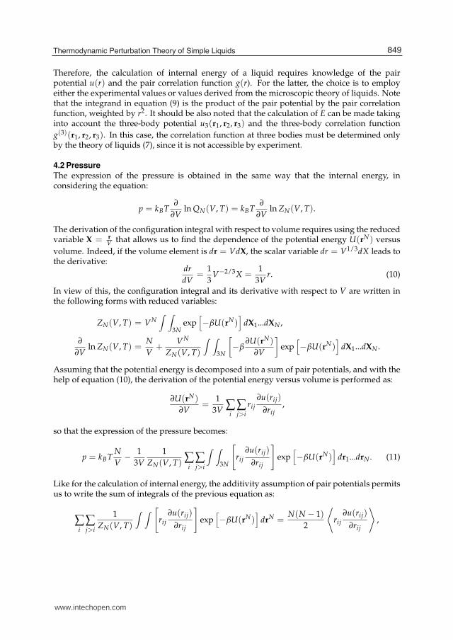
Therefore, the calculation of internal energy of a liquid requires knowledge of the pairpotential u(r) and the pair correlation function g(r). For the latter, the choice is to employeither the experimental values or values derived from the microscopic theory of liquids. Notethat the integrand in equation (9) is the product of the pair potential by the pair correlationfunction, weighted by r2. It should be also noted that the calculation of E can be made takinginto account the three-body potential u3(r1, r2, r3) and the three-body correlation function

g(3)(r1, r2, r3). In this case, the correlation function at three bodies must be determined onlyby the theory of liquids (7), since it is not accessible by experiment.

4.2 Pressure

The expression of the pressure is obtained in the same way that the internal energy, inconsidering the equation:

p = kBT∂

∂Vln QN(V, T) = kBT

∂

∂Vln ZN(V, T).

The derivation of the configuration integral with respect to volume requires using the reducedvariable X = r

V that allows us to find the dependence of the potential energy U(rN) versus

volume. Indeed, if the volume element is dr = VdX, the scalar variable dr = V1/3dX leads tothe derivative:

dr

dV=

1

3V−2/3X =

1

3Vr. (10)

In view of this, the configuration integral and its derivative with respect to V are written inthe following forms with reduced variables:

ZN(V, T) = VN∫ ∫

3Nexp

[

−βU(rN)]

dX1...dXN ,

∂

∂Vln ZN(V, T) =

N

V+

VN

ZN(V, T)

∫ ∫

3N

[

−β∂U(rN)

∂V

]

exp[

−βU(rN)]

dX1...dXN .

Assuming that the potential energy is decomposed into a sum of pair potentials, and with thehelp of equation (10), the derivation of the potential energy versus volume is performed as:

∂U(rN)

∂V=

1

3V ∑i

∑j>i

rij

∂u(rij)

∂rij,

so that the expression of the pressure becomes:

p = kBTN

V−

1

3V

1

ZN(V, T) ∑i

∑j>i

∫ ∫

3N

[

rij

∂u(rij)

∂rij

]

exp[

−βU(rN)]

dr1...drN . (11)

Like for the calculation of internal energy, the additivity assumption of pair potentials permitsus to write the sum of integrals of the previous equation as:

∑i

∑j>i

1

ZN(V, T)

∫ ∫

[

rij

∂u(rij)

∂rij

]

exp[

−βU(rN)]

drN =N(N − 1)

2

⟨

rij

∂u(rij)

∂rij

⟩

,


www.intechopen.com


where the mean value is expressed with the pair correlation function by:

⟨

r12∂u(r12)

∂r12

⟩

= ρ2 (N − 2)!

N!

∫ ∫

6r12

∂u(r12)

∂r12

[

g(2N (r1, r2)

]

dr1dr2.

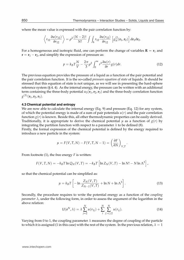
For a homogeneous and isotropic fluid, one can perform the change of variables R = r1 andr = r1 − r2, and simplify the expression of pressure as:

p = kBTN

V−

2π

3ρ2∫ ∞

0r3 ∂u(r)

∂rg(r)dr. (12)

The previous equation provides the pressure of a liquid as a function of the pair potential andthe pair correlation function. It is the so-called pressure equation of state of liquids. It should bestressed that this equation of state is not unique, as we will see in presenting the hard-spherereference system (§ 4. 4). As the internal energy, the pressure can be written with an additionalterm containing the three-body potential u3(r1, r2, r3) and the three-body correlation function

g(3)(r1, r2, r3).

4.3 Chemical potential and entropy

We are now able to calculate the internal energy (Eq. 9) and pressure (Eq. 12) for any system,of which the potential energy is made of a sum of pair potentials u(r) and the pair correlationfunction g(r) is known. Beside this, all other thermodynamic properties can be easily derived.Traditionally, it is appropriate to derive the chemical potential μ as a function of g(r) byintegrating the partition function with respect to a parameter λ to be defined (8).Firstly, the formal expression of the chemical potential is defined by the energy required tointroduce a new particle in the system:

μ = F(V, T, N)− F(V, T, N − 1) =

(

∂F

∂N

)

V,T

.

From footnote (1), the free energy F is written:

F(V, T, N) = −kBT ln QN(V, T) = −kBT[

ln ZN(V, T)− ln N! − N ln Λ3]

,

so that the chemical potential can be simplified as:

μ = kBT

[

− lnZN(V, T)

ZN−1(V, T)+ ln N + ln Λ3

]

. (13)

Secondly, the procedure requires to write the potential energy as a function of the couplingparameter λ, under the following form, in order to assess the argument of the logarithm in theabove relation:

U(rN , λ) = λN

∑j=2

u(r1j) +N

∑i

N

∑j>i≥2

u(rij). (14)

Varying from 0 to 1, the coupling parameter λ measures the degree of coupling of the particleto which it is assigned (1 in this case) with the rest of the system. In the previous relation, λ = 1


www.intechopen.com



means that particle 1 is completely coupled with the other particles, while λ = 0 indicates azero coupling, that is to say the absence of the particle 1 in the system. This allows the writingof the important relations:

U(rN , 1) =N

∑j=2

u(r1j) +N

∑i

N

∑j>i≥2

u(rij) =N

∑i

N

∑j>i≥1

u(rij) = U(rN),

and

U(rN , 0) =N

∑i

N

∑j>i≥2

u(rij) = U(rN−1).

Under these conditions, the configuration integrals for a total coupling (λ = 1) and a zerocoupling (λ = 0) are respectively:

ZN(V, T, λ = 1) =∫ ∫

3Nexp

[

−βU(rN)]

dr1dr2...drN = ZN(V, T), (15)

ZN(V, T, λ = 0) =∫

Vdr1

∫ ∫

3(N−1)exp

[

−βU(rN−1)]

dr2...drN = VZN−1(V, T). (16)

These expressions are then used to calculate the logarithm of the ratio of configurationintegrals in equation (13):

lnZN(V, T)

ZN−1(V, T)= ln

ZN(V, T, λ = 1)

ZN(V, T, λ = 0)+ ln V (17)

= ln V +∫ 1

0

∂ ln ZN

∂λdλ. (18)

But with the configuration integral ZN(V, T, λ), in which potential energy is given by equation

(14), we can easily evaluate the partial derivatives ∂ZN∂λ and ∂ ln ZN

∂λ . In particular, with the result

of the footnote (1), we can write ∂ ln ZN∂λ as a function of the pair correlation function as:

∂ ln ZN(V, T, λ)

∂λ= −βρ2 (N − 1)(N − 2)!

N!

∫ ∫

6u(r12)

{

g(2)N (r1, r2, λ)

}

dr1dr2.

In addition, if the fluid is homogeneous and isotropic, the above relation simplifies under thefollowing form:

∂ ln ZN(V, T, λ)

∂λ= −

βρ2

NV∫ ∞

0u(r)g(r, λ)4πr2dr,

that remains only to be substituted in equation (18) for obtaining the logarithm of the ratio ofconfiguration integrals. And by putting the last expression in equation (13), one ultimatelyarrives to the expression of the chemical potential:

μ = kBT ln ρΛ3 + 4πρ∫ 1

0

∫ ∞

0u(r)g(r, λ)r2drdλ. (19)


www.intechopen.com


Thus, like the internal energy (Eq. 9) and pressure (Eq. 12), the chemical potential (Eq. 19) iscalculated using the pair potential and pair correlation function.Finally, one writes the entropy S in terms of the pair potential and pair correlation function,owing to the expressions of the internal energy (Eq. 9), pressure (Eq. 12) and chemicalpotential (Eq. 19) (cf. footnote 1):

S =E − F

T=

E

T−

μN

T+

pV

T. (20)

It should be noted that the entropy can also be estimated only with the pair correlationfunction g(r), without recourse to the pair potential u(r). The reader interested by this issueshould refer to the original articles (9).

4.4 Application to the hard-sphere potential

In this subsection we determine the equation of state of the hard-sphere system, of which thepair potential being:

u(r) =

⎧

⎨

⎩

∞ if r < σ

0 if r > σ,

where σ is the hard-sphere diameter. The Boltzmann factor associated with this potential has asignificant feature that enable us to express the thermodynamic properties under particularlysimple forms. Indeed, the representation of the Boltzmann factor

exp [−βu(r)] =

⎧

⎨

⎩

0 if r < σ

1 if r > σ,

is a step function (Fig. 4) whose derivative with respect to r is the Dirac delta function, i. e.:

∂

∂rexp [−βu(r)] = −β

∂u

∂rexp [−βu(r)] = δ(r − σ).

In substituting ∂u∂r , taken from the previous relation, in equation (12) we find the expression of

the pressure:

p = kBTN

V−

2π

3ρ2∫ ∞

0r3

{

−1

β

δ(r − σ)

exp [−βu(r)]

}

g(r)dr,

or:

p = kBTN

V+

2π

3kBTρ2σ3g(σ) exp [βu(σ)] . (21)

It is important to recall that, for moderately dense gases, the pressure is usually expressedunder the form of the virial expansion

p

ρkBT= 1 + ρB2(T) + ρ2B3(T) + ρ3B4(T) + ... =

pGP

ρkBT+

pex

ρkBT.


www.intechopen.com



Fig. 4. Representation of the hard-sphere potential and its Boltzmann factor.

The first term of the last equality represents the contribution of the ideal gas, and the excesspressure pex comes from the interactions between particles. They are written:

pGP

ρkBT= 1,

andpex

ρkBT= 4η + η2B′

3(T) + η3B′4(T) + ...

where η is the packing fraction defined by the ratio of the volume actually occupied by the Nspherical particles on the total volume V of the system, that is to say:

η =1

V

4π

3

(σ

2

)3N =

π

6ρσ3. (22)

Note that the first 6 coefficients of the excess pressure pex have been calculated analyticallyand by molecular dynamics (10), with great accuracy. In addition, Carnahan and Starling(11) have shown that the excess pressure of the hard-sphere fluid can be very well predictedby rounding the numerical values of the 6 coefficients towards the nearest integer values,according to the expansion:

pex

ρkBT≃ 4η + 10η2 + 18η3 + 28η4 + 40η5 + 54η6... ≃

∞

∑k=1

(k2 + 3k)ηk. (23)


www.intechopen.com


In combining the first and second derivatives of the geometric series ∑∞k=1 ηk, it is found that

equation (23) can be transformed into a rational fraction5 enabling the deduction of the excesspressure in the form:

pex

ρkBT≃

∞

∑k=1

(k2 + 3k)ηk =4η − 2η2

(1 − η)3.

Consequently, the equation of state of the hard-sphere fluid is written with excellent precisionas:

p

ρkBT=

1 + η + η2 − η3

(1 − η)3. (24)

It is also possible to calculate the internal energy of the hard-sphere fluid by substituting u(r)in equation (9). Given that u(r) is zero when r > σ and g(r) is zero when r < σ, it followsthat the integral is always zero, and that the internal energy of the hard-sphere fluid is equal

to that of the ideal gas E = 32 NkBT.

As for the free energy F, it is determined by integrating the pressure over volume with theequation:

p = −

(

∂F

∂V

)

T

= −

(

∂FGP

∂V

)

T

−

(

∂Fex

∂V

)

T

,

where FGP is the free energy of ideal gas (cf. footnote 1, with ZN(V, T) = VN):

FGP = NkBT(

ln ρΛ3 − 1)

,

and Fex the excess free energy, calculated by integrating equation (23) as follows:

Fex = −∫

pexdV = −∫

NkBT

V

(

4η + 10η2 + 18η3 + 28η4 + 40η5 + 54η6...) dV

dηdη.

5 To obtain the rational fraction, one must decompose the sum as:

∞

∑k=1

(k2 + 3k)ηk =∞

∑k=1

(k2 − k)ηk +∞

∑k=1

4kηk ,

and combine the geometric series ∑∞k=1 ηk with its first and second derivatives:

∞

∑k=1

ηk = η + η2 + η3 + ... =η

1 − η,

∞

∑k=1

kηk−1 =1

(1 − η)2,

and∞

∑k=1

k(k − 1)ηk−2 =2

(1 − η)3,

to see appear the relation:∞

∑k=1

(k2 + 3k)ηk =2η2

(1 − η)3+

4η

(1 − η)2.


www.intechopen.com



But, with equation (22) that gives dVdη = −V

η , Fex is then reduced to the series expansion:

Fex

NkBT= 4η + 5η2 + 6η3 + 7η4 + 8η5 + 9η6... =

∞

∑k=1

(k + 3)ηk.

Like the pressure, this expansion is written as a rational function by combining the geometric

series ∑∞k=1 ηk with its first derivative6. The expression of the excess free energy is:

Fex

NkBT=

∞

∑k=1

(k + 3)ηk =4η − 3η2

(1 − η)2,

and the free energy of the hard-sphere fluid reduces to the following form:

F

NkBT=

FGP

NkBT+

Fex

NkBT= ln ρΛ3 − 1 +

4η − 3η2

(1 − η)2. (25)

Now, the entropy is obtained using the same method of calculation, by deriving the freeenergy with respect to temperature:

S = −

(

∂F

∂T

)

V

= −

(

∂FGP

∂T

)

V

−

(

∂Fex

∂T

)

V

,

where SGP is the entropy of the ideal gas given by the Sackur-Tetrode equation:

SGP = −NkB

(

ln ρΛ3 −5

2

)

,

and where the excess entropy Sex arises from the relation:

Sex = −

(

∂Fex

∂T

)

V

= −NkB4η − 3η2

(1 − η)2,

hence the expression of the entropy of the hard-sphere fluid:

S

NkB= − ln ρΛ3 +

5

2−

4η − 3η2

(1 − η)2. (26)

Finally, combining equations (25) and (24), with the help of equation (20), one reaches thechemical potential of the hard-sphere fluid that reads:

μ

kBT=

F

NkBT+

p

ρkBT= ln ρΛ3 − 1 +

1 + 5η − 6η2 + 2η3

(1 − η)3. (27)

6 Indeed, the identity:∞

∑k=1

(k + 3)ηk =∞

∑k=1

kηk +∞

∑k=1

3ηk ,

is yet written:∞

∑k=1

(k + 3)ηk =η

(1 − η)2+

3η

(1 − η),


www.intechopen.com


Since they result from equation (23), the expressions of thermodynamic properties (p, F, S andμ) of the hard-sphere fluid make up a homogeneous group of relations related to the Carnahanand Starling equation of state. But other expressions of thermodynamic properties can alsobe determined using the pressure equation of state (Eq. 12) and the compressibility equationof state, which will not be discussed here. Unlike the Carnahan and Starling equation ofstate, these two equations of state require knowledge of the pair correlation function of hardspheres, gHS(r). The latter is not available in analytical form. The interested reader will findthe Fortran program aimed at doing its calculation, in the book by McQuarrie (12), page 600.It should be mentioned that the thermodynamic properties (p, F, S and μ), obtained with theequations of state of pressure and compressibility, have analytical forms similar to those fromthe Carnahan and Starling equation of state, and they provide results whose differences areindistinguishable to low densities.

5. Thermodynamic perturbation theory

All theoretical and experimental studies have shown that the structure factor S(q) of simpleliquids resembles that of the hard-sphere fluid. For proof, just look at the experimentalstructure factor of liquid sodium (13) at 373 K, in comparison with the structure factor ofhard-sphere fluid (14) for a value of the packing fraction η of 0.45. We can see that theagreement is not bad, although there is a slight shift of the oscillations and ratios of peakheights significantly different. Besides, numerical calculations showed that the structurefactor obtained with the Lennard-Jones potential describes the structure of simple fluids (15)and looks like the structure factor of hard-sphere fluid whose diameter is chosen correctly.

Fig. 5. Experimental structure factor of liquid sodium at 373 K (points), and hard-spherestructure factor (solid curve), with η = 0, 45.


www.intechopen.com



Such a qualitative success emphasizes the role played by the repulsive part of the pairpotential to describe the structure factor of liquids, while the long-ranged attractivecontribution has a minor role. It can be said for simplicity that the repulsive contributionof the potential determines the structure of liquids (stacking of atoms and steric effects) andthe attractive contribution is responsible for their cohesion.It is important to remember that the thermodynamic properties of the hard-sphere fluid (Eqs.24, 25, 26, 27) and the structure factor SHS(q) can be calculated with great accuracy. Thatsuggests replacing the repulsive part of potential in real systems by the hard-sphere potentialthat becomes the reference system, and precict the structural and thermodynamic propertiesof real systems with those of the hard-sphere fluid, after making the necessary adaptations.To perform these adaptations, the attractive contribution of potential should be treated as aperturbation to the reference system.The rest of this subsection is devoted to a summary of thermodynamic perturbation methods7.It should be noted, from the outset, that the calculation of thermodynamic properties with thethermodynamic perturbation methods requires knowledge of the pair correlation functiongHS(r) of the hard-sphere system and not that of the real system.

5.1 Zwanzig method

In perturbation theory proposed by Zwanzig (16), it is assumed that the total potential energyU(rN) of the system can be divided into two parts. The first part, U0(r

N), is the energy ofthe unperturbed system considered as reference system and the second part, U1(r

N), is theenergy of the perturbation which is much smaller that U0(r

N). More precisely, it is posed thatthe potential energy depend on the coupling parameter λ by the relation:

U(rN) = U0(rN) + λU1(r

N)

in order to vary continuously the potential energy from U0(rN) to U(rN), by changing λ from

0 to 1, and that the free energy F of the system is expanded in Taylor series as:

F = F0 + λ

(

∂F

∂λ

)

+λ2

2

(

∂2F

∂λ2

)

+ ... (28)

By replacing the potential energy U(rN) in the expression of the configuration integral (cf.footnote 1), one gets:

ZN(V, T) =∫ ∫

3Nexp

[

−βU0(rN)]

drN ×

∫ ∫

3N

{

exp[

−βλU1(rN)]}

exp[

−βU0(rN)]

drN

∫ ∫

3N exp [−βU0(rN)] drN.

The first integral represents the configuration integral Z(0)N (V, T) of the reference system, and

the remaining term can be regarded as the average value of the quantity exp[

−βλU1(rN)]

, sothat the previous relation can be put under the general form:

ZN(V, T) = Z(0)N (V, T)

⟨

exp[

−βλU1(rN)]⟩

0, (29)

where 〈...〉0 refers to the statistical average in the canonical ensemble of the reference system.After the substitution of the configuration integral (Eq. 29) in the expression of the free energy

7 The interested reader will find all useful adjuncts in the books either by J. P. Hansen and I. R. McDonaldor by D. A. McQuarrie.


www.intechopen.com


(cf. footnote 1), this one reads:

− βF = lnZ(0)N (V, T)

N!Λ3N+ ln

⟨

exp[

−βλU1(rN)]⟩

0. (30)

The first term on the RHS stands for the free energy of the reference system, denoted (−βF0),and the second term represents the free energy of the perturbation:

− βF1 = ln⟨

exp[

−βλU1(rN)]⟩

0. (31)

Since the perturbation U1(rN) is small, exp (−βλU1) can be expanded in series, so that the

statistical average⟨

exp[

−βλU1(rN)]⟩

0, calculated on the reference system, is expressed as:

⟨

exp[

−βλU1(rN)]⟩

0= 1 − βλ 〈U1〉0 +

1

2!β2λ2

⟨

U21

⟩

0−

1

3!β3λ3

⟨

U31

⟩

0+ ... (32)

Incidentally, we may note that the coefficients of β in the preceding expansion representstatistical moments in the strict sense. Given the shape of equation (32), it is stillpossible to write equation (31) by expanding ln

⟨

exp[

−βλU1(rN)]⟩

0 in Taylor series. Aftersimplifications, equation (31) reduces to:

ln⟨

exp[

−βλU1(rN)]⟩

0= −βλ 〈U1〉0 +

1

2!β2λ2

[⟨

U21

⟩

0− 〈U1〉

20

]

−β3λ3

[

1

3!

⟨

U31

⟩

0−

1

2〈U1〉0

⟨

U21

⟩

0+

1

3〈U1〉

30

]

+ β4λ4 [...]− ...

Now if we set:

c1 = 〈U1〉0 , (33)

c2 =1

2!

[⟨

U21

⟩

0− 〈U1〉

20

]

, (34)

c3 =1

3!

[⟨

U31

⟩

0− 3 〈U1〉0

⟨

U21

⟩

0+ 2 〈U1〉

30

]

, etc. (35)

we find that:ln⟨

exp[

−βλU1(rN)]⟩

0= −λβc1 + λ2β2c2 − λ3β3c3 + ...

The contribution of the perturbation (Eq. 31) to the free energy is then written in the compactform:

− βF1 = ln⟨

exp[

−βλU1(rN)]⟩

0= −λβ

∞

∑n=1

cn(−λβ)n−1, (36)

and the expression of the free energy F of the real system is found by substituting equation(36) into equation (30), as follows:

F = F0 + F1 = F0 + λc1 − λ2βc2 + λ3β2c3 + ..., (37)

where the free energy of the real system is obtained by putting λ = 1. This expression ofthe free energy of liquids in power series expansion of β corresponds to the high temperatureapproximation.


www.intechopen.com



5.2 Van der Waals equation

As a first application of thermodynamic perturbation method, we search thephenomenological van der Waals equation of state. In view of this, consider equation(37) at zero order in β. The simplest assumption to determine c1 is to admit that the totalpotential energy may be decomposed into a sum of pair potentials in the form:

U(rN) = U0(rN) + U1(r

N) = ∑i

∑j>i

u0(rij) + ∑i

∑j>i

u1(rij).

Therefore, the free energy of the perturbation to zero order in β is given by equation (33), thatis to say:

c1 = 〈U1〉0 =

∫ ∫

3N

[

∑i ∑j>i u1(rij)]

exp[

−βU0(rN)]

drN

∫ ∫

3N exp [−βU0(rN)] drN.

To simplify the above relation, we proceed as for calculating the internal energy of liquids(Eq. 8) by revealing the pair correlation function of the reference system in the numerator.If we assume that the sum of pair potentials is composed of equivalent terms equal to

∑i ∑j>i u1(rij) =N(N−1)

2 u1(r12), the expression of c1 is simplified as:

c1 =1

Z0(V, T)

∫ ∫

N(N − 1)

2u1(r12)

{

∫ ∫

3(N−2)exp

[

−βU0(rN)]

dr3...drN

}

dr1dr2.

The integral in between the braces is then expressed as a function of the pair correlationfunction (cf. footnote 2), and c1 reduces to:

c1 =ρ2

2

∫

dR

∫

u1(r)g0(r)dr. (38)

Yet, to find the equation of van der Waals we have to choose the hard-sphere system ofdiameter σ, as reference system, and suppose that the perturbation is a long-range potential,weakly attractive, the form of which is not useful to specify (Fig. 6a). Since one was unawareof the existence of the pair correlation function when the model was developed by van derWaals, it is reasonable to estimate g0(r) by a function equal to zero within the particle, and toone at the outside. According to van der Waals, suppose further that the available volume per

particle8 is b = 23 πσ3 and the unoccupied volume is (V − Nb).

With these simplifications in mind, the configuration integral and free energy of the referencesystem are respectively (cf. footnote 1):

Z0(V, T) =∫ ∫

3Nexp

[

−βU0(rN)]

drN = (V − Nb)N ,

and F0 = −kBT ln

[

(V − Nb)N

N!Λ3N

]

= −NkBT

[

ln(V − Nb)

N− 3 ln Λ + 1

]

.

8 The parameter b introduced by van der Waals is the covolume. Its expression comes from the fact that

if two particles are in contact, half of the excluded volume 43 πσ3 must be assigned to each particle (Fig.

6b).


www.intechopen.com


Fig. 6. Schematic representation of the pair potential by a hard-sphere potentiel plus a

perturbation. (b) Definition of the covolume by the quantity b = 12

(

43 πσ3

)

.

As for the coefficient c1 (Eq. 38), it is simplified as:

c1 = 2πρ2V∫ ∞

σu1(r)r

2dr = −aρN, (39)

with a = −2π∫ ∞

σu1(r)r

2dr.

Therefore, the expression of free energy (Eq. 37) corresponding to the model of van der Waalsis:

F = F0 + c1 = −NkBT

[

ln(V − Nb)

N− 3 ln Λ + 1

]

− aρN,

and the van der Waals equation of state reduces to:

p = −

(

∂F

∂V

)

T

=NkBT

V − Nb− a

N

V2

2

.

With b = a = 0 in the previous equation, it is obvious that one recovers the equation of stateof ideal gas. In return, if one wishes to improve the quality of the van der Waals equationof state, one may use the expression of the free energy (Eq. 25) and pair correlation functiongHS(r) of the hard-sphere system to calculate the value of the parameter a with equation (38).Another way to improve performance is to calculate the term c2. Precisely what will be donein the next subsection.

5.3 Method of Barker and Henderson

To evaluate the mean values of the perturbation U1(rN) in equations (34) and (35), Barker and

Henderson (17) suggested to discretize the domain of interatomic distances into sufficientlysmall intervals (r1, r2) , (r2, r3) , ..., (ri, ri+1),..., and assimilate the perturbating elementalpotential in each interval by a constant. Assuming that the perturbating potential in theinterval (ri, ri+1) is u1(ri) and that the number of atoms subjected to this potential is Ni, thetotal perturbation can be written as the sum of elemental potentials:


www.intechopen.com



U1(rN) = ∑

i

Niu1(ri),

before substituting it in the configuration integral. The advantage of this method is to calculatethe coefficients cn and free energy (Eq. 37), not with the mean values of the perturbation, butwith the fluctuation number of particles. Thus, each perturbating potential u1(ri) is constant

in the interval which it belongs, so that we can write 〈U1〉20 = ∑i ∑j〈Ni〉0〈Nj〉0u1(ri)u1(rj). In

view of this, the coefficient c2 defined by equation (34) is:

c2 =1

2!

[⟨

U21

⟩

0− 〈U1〉

20

]

=1

2! ∑i

∑j

[⟨

Ni Nj

⟩

0− 〈Ni〉0

⟨

Nj

⟩

0

]

u1(ri)u1(rj).

With the local compressibility approximation (LC), where ρ and g0 depend on p, the expressionof c2 obtained by Barker and Henderson according to the method described above is written:

c2(LC) =πNρ

β

(

∂ρ

∂p

)

0

∂

∂ρ

[

∫

ρu21(r)g0(r)r

2dr

]

. (40)

Incidentally, note the macroscopic compressibility approximation (MC), where only ρ is assumedto be dependent on p, has also been tested on a system made of the hard-sphere referencesystem and the square-well potential as perturbation. At low densities, the results of bothapproximations are comparable. But at intermediate densities, the results obtained withthe LC approximation are in better agreement with the simulation results than the MCapproximation. Note also that the coefficient c3 has been calculated by Mansoori and Canfield(18) with the macroscopic compressibility approximation.At this stage of the presentation of the thermodynamic perturbation theory, we are in positionto calculate the first terms of the development of the free energy F (Eq. 37), using thehard-sphere system as reference system. But there is not yet a criterion for choosing thediameter d of hard spheres. This point is important because all potentials have a repulsivepart that must be replaced by a hard-sphere potential of diameter properly chosen. Decisiveprogress has been made to solve this problem in three separate ways followed, respectively, byBarker and Henderson (19), Mansoori and Canfield (20) and Week, Chandler and Andersen(21).Prescription of Barker and Henderson. To choose the best reference system, that is to say,the optimal diameter of hard spheres, Barker and Henderson (19) proposed to replace thepotential separation u(r) = u0(r) + λu1(r), where u0(r) is the reference potential, u1(r)the perturbation potential and λ the coupling parameter, by a more complicated separationassociated with a potential v(r) whose the Boltzmann factor is:

exp [−βv(r)] =

[

1 − Ξ

(

d +r − d

α− σ

)]

exp

[

−βu(d +r − d

α)

]

+ Ξ

(

d +r − d

α− σ

)

+ Ξ (r − σ) {exp [−βλu(r)]− 1} , (41)

where Ξ(x) is the Heaviside function, which is zero when x < 0 and is worth one whenx > 0. Note that here σ is the value of r at which the real potential u(r) vanishes and d is thehard-sphere diameter of the reference potential, to be determined. Moreover, the parametersλ and α are coupling parameters that are 0 or 1. If one looks at equation (41) at the same timeas figure(7a), it is seen that the function v(r) reduces to the real potential u(r) when α = λ = 1,


www.intechopen.com


Fig. 7. Separation of the potential u(r) according to (a) the method of Barker and Hendersonand (b) the method of Weeks, Chandler and Andersen.

and it behaves approximately as the hard-sphere potential of diameter d when α ∼ λ ∼ 0.The substitution of equation (41) in the configuration integral (Eq. 29), followed by the relatedcalculations not reproduced here, enable us to express the free energy F of the real systemas a series expansion in powers of α and λ, which makes the generalization of equation (28),namely:

F = FHS + λ

(

∂F

∂λ

)

+ α

(

∂F

∂α

)

+λ2

2

(

∂2F

∂λ2

)

+α2

2

(

∂2F

∂α2

)

+ ... (42)

By comparing equations (37) and (42), we see that the first derivative(

∂F∂λ

)

coincides with c1

and the second derivative 12

(

∂2 F∂λ2

)

with (−βc2). Concerning the derivatives of F with respect

to α, they are complicated functions of the pair potential and the pair correlation function

of the hard-sphere system. The first derivative(

∂F∂α

)

, whose the explicit form given without

proof, reads:

(

∂F

∂α

)

= −2πNρkBTd2gHS(d)

[

d −∫ σ

0{1 − exp [−βu(r)]} dr

]

.

Since the Barker and Henderson prescription is based on the proposal to cancel the term(

∂F∂α

)

,

the criterion for choosing the hard-sphere diameter d is reduced to the following equation:

d =∫ σ

0{1 − exp [−βu(r)]} dr. (43)

In applying this criterion to the Lennard-Jones potential, it is seen that d depends ontemperature but not on the density. Also, the calculations show that the terms of the expansion

of F in α2 and αλ are negligible compared to the term in λ2.


www.intechopen.com



Therefore, using equation (38) to evaluate c1 and equation (40) to evaluate c2, the expressionof the free energy F of the real system (Eq. 42) is:

F = FHS + 2πρN∫ ∞

du1(r)gHS(η; r)r2dr

− πNρ

(

∂ρ

∂p

)

HS

∂

∂ρ

[

∫ ∞

dρu2

1(r)gHS(η; r)r2dr

]

, (44)

where the first term on the RHS represents the free energy of the hard-sphere system (Eq. 25),

and the partial derivative(

∂ρ∂p

)

HScan be deduced from the Carnahan and Starling equation of

state (Eq. 24). Recall that the pair correlation function of hard-sphere system, gHS(η; r), mustbe only determined numerically. It depends on the density ρ and diameter d via the packingfraction η(= π

6 ρd3). Since gHS(η; r) = 0 when r < d, either 0 or d can be used as lower limitof integration in equation (44).

5.4 Prescription of Mansoori and Canfield.

An important consequence of the high temperature approximation to first order in β is to markout the free energy of the real system by an upper limit that can not be exceeded, because thesum of the terms beyond c1 is always negative. The easiest way to proof this, is to consider theexpression of the free energy (Eq. 30) and to write the perturbation U1(r

N) around its meanvalue 〈U1〉0 as:

U1 = 〈U1〉0 + ΔU1.

After replacing U1 in equation (30), we obtain:

− βF = −βF0 − β 〈U1〉0 + ln⟨

exp [−βΔU1]0⟩

. (45)

However, considering the series expansion of an exponential, the above relation istransformed into the so-called Gibbs-Bogoliubov inequality9:

F ≤ F0 + 〈U1〉0 . (46)

A thorough study of this inequality shows that it is always valid, and it is unnecessary toconsider values of n greater than zero. Equation (46), at the base of the variational method,allows us to find the value of the parameter d that makes the free energy F minimum. If thereference system is that of hard spheres, the value of the free energy obtained with this valueof d (or η = π

6 ρd3) is considered as the best estimate of the free energy of the real system. Itsexpression is:

F ≤ FHS +ρN

2

∫

u1(r)gHS(η; r)dr, (47)

9 The Mac-Laurin series of the exponential naturally leads to the inequality:

exp (−βΔU1) ≥2n+1

∑k=0

(−βΔU1)k

k!(n = 0, 1, 2, ...).

For n = 0, the last term of equation (45) behaves as:

ln

⟨

1

∑k=0

(−βΔU1)k

k!

⟩

0

= ln 〈1 − βΔU1〉0 ≃ −β 〈ΔU1〉0 = 0,

since the mean value of the deviation, 〈ΔU1〉0 , is zero.


www.intechopen.com


where F0 = FHS is given by equation (25) and 〈U1〉0 = c1 by equation (38). Since gHS(η; r) = 0when r < d and u1(r) = u(r)− uHS(r) = u(r) when r ≥ d, equation (47) can be written as:

F ≤ FHS + 2πρN∫ ∞

0u(r)gHS(η; r)r2dr. (48)

Practically, we vary the value of d (or η) until the result of the integral is minimum. And thevalue of F thus obtained is the best estimate of the free energy of the real system, in the sensof the variational method (20).

5.5 Prescription of Weeks, Chandler and Andersen.

At the same time that the perturbation theory was developing, Weeks, Chandler andAndersen (21) formulated another prescription for finding the hard-sphere diameter d. Itsoriginality lies in the idea that a particle in the liquid is less sensitive to the sign of thepotential u(r) than to the sign of the strength, that is to say, to the derivative of the potential(

− ∂u∂r

)

ρ,T. That is why the authors proposed to separate the real potential into a purely

repulsive contribution and a purely attractive perturbation. This separation, shown in figure(7b), is defined by the relation u(r) = u0(r) + u1(r) with:

u0(r) =

{

u(r) + ε if r < rmin

0 if r ≥ rmin

u1(r) =

{

−ε if r < rmin

u(r) if r ≥ rmin,

where ε is the depth of the potential well, i. e. the value of u(rmin) = −ε.To follow the same sketch that for the Barker and Henderson prescription, define the potentialv(r) by the Boltzmann factor:

exp [−βv(r)] = exp [−βuHS(d)] + α {exp [−β (u0(r) + λu1(r))]− exp [−βuHS(d)]} . (49)

However, from the simultaneous observation of equation (49) and figure (7b) one remarksthat the potential v(r) reduces to the real potential u(r) when α = λ = 1, and behaves like thehard-sphere potential of diameter d when α = 0.The substitution of equation (49) in the configuration integral, and subsequent calculations,enables us to express the free energy F of the system as a series expansion in powers of α andλ identical to that of equation (42). The first term of this expansion, FHS, is the free energy ofthe hard-sphere system. As for the first derivative of F with respect to α, it is written in thiscase:

(

∂F

∂α

)

= −2πNρ

β

∫ ∞

0{exp [−βu0(r)]− exp [−βuHS(d)]} yHS(η; r)r2dr, (50)

where yHS(η; r) is the cavity function of great importance in the microscopic theory of liquids10.It is defined by means of the pair correlation function gHS(η; r) and the Boltzmann factorexp [−βuHS(d)] of the hard-sphere potential as:

yHS(η; r) = exp [βuHS(d)] gHS(η; r). (51)

10 The cavity function yHS(η; r) does not exist in analytical form. It must be calculated at all reduceddensities (ρd3) by solving an integro-differential equation.


www.intechopen.com



It should be stressed that the cavity function depends only weakly on the potential, this is whyWeeks, Chander and Anderson (WCA) suggested to use the same cavity function yHS(η; r) forall potentials, and to express the pair correlation functions of each potential as a function ofyHS(η; r). As a result, the pair correlation function g0(r) related to the repulsive contributionu0(r) of the potential can be approximately written as:

g0(r) ≃ exp [−βu0(r)] yHS(η; r). (52)

The suggestion of WCA for choosing the hard-sphere diameter d is to cancel(

∂F∂α

)

, which

amounts to solving the nonlinear equation given by equation (50), i. e.:

∫ ∞

0{exp [−βu0(r)]− exp [−βuHS(d)]} yHS(η; r)r2dr = 0. (53)

It is interesting to note that equation (53) has a precise physical meaning that appears bywriting it in terms of the pair correlation functions gHS(η; r) and g0(r) drawn, respectively,from equations (51) and (52). It reads:

∫ ∞

0[g0(r)− 1] r2dr =

∫ ∞

0[gHS(η; r)− 1] r2dr.

According to equation (7), the previous expression is equivalent to the equality S0(0) =SHS(0), meaning the equality between the isothermal compressibility of the repulsivepotential u0(r) and that of the hard-sphere potential uHS(d).Ultimately, the expression of free energy (Eq. 28) of the real system is the sum of FHS,

calculated with the value of d issued from equation (53), and the term(

∂F∂λ

)

= c1, calculated

with equation (38) in using the pair correlation function g0(r) ≃ exp [−βu0(r)] yHS(η; r), i. e.:

F = FHS + 2πρN∫ ∞

0u1(r) {exp [−βu0(r)] yHS(η; r)} r2dr. (54)

Note that the value of d obtained with the WCA prescription (blip function method) issignificantly larger than that obtained with the Barker and Henderson (BH) prescription.By the fact that yHS(η; r) depends on density, the value of d calculated with equation (53)depends on temperature and density, while that calculated with equation (43) depends onlyon temperature.In order to compare the relative merits of equations (44) and (54), simply note that the WCAprescription shows that not only the terms of the expansion of F in α2 and in αλ are negligible,

but also the term in λ2. This means that the WCA treatment is a theory of first order in λ, whilethe BH one is a theory of second order in λ. In addition, the BH treatment is coherent as FHS,c1 and c2 are calculated with the same reference system, whereas the WCA treatment is notcoherent because it uses the hard-sphere system to calculate FHS and the repulsive potentialu0(r) to calculate c1, via the pair correlation function g0(r). In contrast, the WCA treatmentdoes not require the calculation of c2 and improves the convergence of calculations. As anadditional advantage, the WCA treatment can be used to predict the structure factor of simpleliquids (22).


www.intechopen.com


5.6 Application to the Yukawa attractive potential

As an application of the perturbation theory, consider the hard-core attractive Yukawapotential (HCY). This potential consists of the hard-sphere potential uHS(d) and the attractiveperturbation u1(r). Its traditional analytical form is:

u(r) =

{

∞

−(εd/r) exp[−λ(r/d − 1)]r < dr ≥ d,

(55)

where d is the diameter of hard spheres, ε the potential value at r = d and λ a parameter thatmeasures the rate of exponential decay. The shape of this potential is portrayed in figure (8a)

Fig. 8. (a) Representation of the HCY potential for three values of λ (1.8, 3.0, 4.0). (b) Phasediagram of the HCY potential for the same three values of λ (1.8, 3.0, 4.0).

for three different values of λ. For guidance, note that a value of λ ∼ 1.8 predicts thethermodynamic properties of liquid rare gases quite so well as the Lennard-Jones potential.By contrast, a value of λ ∼ 8 enables us to obtain the thermodynamic properties of colloidalsuspensions or globular proteins. This wide possible range of λ values explains why the HCYpotential has been used in many applications and has been the subject of numerous theoreticalstudies after its analytical solution was obtained by Waisman (2). Without going into details ofthe resolution of the problem that involves the microscopic theory of liquids, indicate that thesolution reduces to determining a fundamental parameter Γ as the root of the quartic equation(23):

Γ(1 + λΓ)(1 + ψΓ)2 + βεw = 0, (56)

where ε and λ are the two parameters of the HCY potential, and w and ψ two additionalparameters explicitly depending on λ and η by the following relations:

w =6η

φ20

,

ψ = λ2(1 − η)2 [1 − exp(−λ)]

L(λ) exp(−λ) + S(λ)

−12η(1 − η)[1 − λ/2 − (1 + λ/2) exp(−λ)]

L(λ) exp(−λ) + S(λ),


www.intechopen.com



with:

φ0 =L(λ) exp(−λ) + S(λ)

λ3(1 − η)2,

L(λ) = 12η[1 + 2η + (1 + η/2)λ],

S(λ) = (1 − η)2λ3 + 6η(1 − η)λ2 + 18η2λ − 12η(1 + 2η).

By expressing Γ as a function of β, Henderson et al. (3) managed to write the free energy F ofthe system according to the series expansion in powers of β:

F = FHS −NkBT

2

∞

∑n=1

vn

n(βε)n , (57)

where FHS is the free energy of the hard-sphere system calculated, for example, with equation(25), and where the first five terms vn have expressions derived by the authors11.At this stage, we see that the free energy of the HCY potential can be approximated for allvalues of the triplet (η, ε, λ), using the analytical expressions of the five coefficients vn givenin footnote (11). From equation (57), we can also deduce the internal energy (Eq. 9), excesspressure (Eq. 12), chemical potential (Eq. 19) and entropy (Eq. 20) of the HCY system.The HCY equation of state, which is based on the perturbation theory and expressedin terms of the relevant features of the potential, is a very handy tool for investigatingthe thermodynamics of systems governed by an effective hard-sphere interaction plus anattractive tail. Alternatively, the HCY system could be used vicariously to approximate anyavailable interatomic potential for real fluids.

The reduced phase diagrams (T∗ = kBTε versus ρ∗ = ρσ3 =

6ηπ ) predicted by this equation

of state, for values of λ = 1.8, 3 and 4, are displayed in figure (8b), together with simulationdata. A rapid glance at figure (8b) indicates that the critical temperature T∗

C predicted by theperturbation theory is noticeably greater than that predicted by the simulation. The reason isthat the HCY equation of state involves a truncated series. But, also, we can speculate that the

11 The first terms of the series expansion are:

v0 = 0,

v1 =2α0

φ0

,

v2 =2w(1 − α1 + α0ψ)

λφ0

,

v3 =2w2(1 − α1 + α0ψ) (1 + 3λψ)

λ3φ0

,

v4 =4w3(1 − α1 + α0ψ)

(

1 + 4λψ + 6λ2ψ2)

λ5φ0

,

v5 =10w4(1 − α1 + α0ψ)

(

1 + 5λψ + 11λ2ψ2 + 11λ3ψ3)

λ7φ0

,

with:

α0 =L(λ)

λ2(1 − η)2; α1 =

12η(1 + λ/2)

λ2(1 − η)and (1 − α1 + α0ψ)φ0 = 1.


www.intechopen.com


correlation functions, inherent in the calculations of the pressure and the chemical potential,do not represent correctly the growing correlation lengths in approaching the critical point.Looking at the evolution of the binodal lines as a function of the rate of decay λ of the Yukawapotential, we remark that higher the critical temperature is, lower λ is. At the same time, thedomain below the binodal line shrinks. In contrast, when λ increases (i. e., the attractionrange of the potential becomes shorter), the critical temperature decreases, and the liquid andgaseous phases become indistinguishable. For the hard-sphere potential, as a border case(λ → ∞), there is no longer gas-liquid phase transition. On the other hand, one can see thatthe phase diagrams obtained with the perturbation theory agree with simulation data morefavorably for the vapor branch than for the liquid branch. This is not surprising in the extentthat the perturbation theory works better for low densities. Lastly, it should be mentionedthat the structure and thermodynamic properties of the HCY potential have been extensivelystudied for the two last decades, as much by computer simulations and integral equationtheory as by means of perturbation theory. Note that many other studies of the HCY potentialwith these various methods are available in literature (24).

6. Concluding remarks

In the foregoing, we started with a brief discussion of the liquid state, compared withthe gaseous and solid states. Among other things, we mentioned that one of the mostsuccesses of the microscopic theory of liquids has been to emphasize the importance of thepair potential u(r) to describe a wide variety of physical properties of liquids. Then, welearned a rudimentary knowledge of the structure of liquids. The latter is essentially describedby the static structure factor S(q), which can be measured directly by elastic scattering ofneutrons or X-rays. But S(q), or more precisely the pair correlation function g(r), can alsobe determined by numerical simulations (known as virtual experiments) and with modelsof the microscopic theory of liquids once the nature of the pair potential u(r) is known. Thecomparison between simulation results and those of analytical models essentially allows usto test the models, whereas the comparison of simulation results with experimental results isthe ultimate test to judge the efficiency of the pair potential. Subsequently, we described inminute detail the calculations of the thermodynamic properties in terms of the pair potentialand pair correlation function. In particular, with the pressure p and the chemical potentialμ to apply equilibrium conditions, it has been shown that we are in a position to determinetheoretical estimates for the liquid-vapor coexistence curve. Finally, we got down to basics ofthe thermodynamic perturbation theory, before presenting the liquid-vapor coexistence curvefor the HCY fluid.In a 1990 time warp, it became apparent that the usefulness of thermodynamic perturbationtheory was on the decline compared to the more powerful simulation methods. Thiswas primarily due to the rapid increase in the power of computers. At the same time,the integral equation theory enjoyed renewed popularity with the extensively employedconcept of thermodynamic consistency (25), but this aspect goes beyond the scope ofthis short review. Incidentally, we recall that the thermodynamic consistency consists toadjusting the isothermal compressibility obtained by two different routes. Nevertheless, thethermodynamic perturbation theory remains undoubtedly the most tractable approach topredict the thermodynamic properties of liquids. Let us just quote few articles containinginvestigations of the HCY fluid with the integral equation theory (26).As one would expect, the thermodynamic perturbation theory described previously is alsoimportant for mixtures. The thermodynamic properties established for studying pure liquidscan be applied to binary mixtures, with only few modifications. Specifically, analytic


www.intechopen.com



expressions for the hard-sphere free energy FHS(d1, d2) and subsequent thermodynamicquantities are readily generalized for a mixture of hard spheres of different diameters d1 andd2. Therefore, if one estimates that a real binary mixture behaves like binary hard-spherefluid, the variational method consists of minimizing FHS(d1, d2) versus the two hard-spherediameters, and by taking the resulting minimum upper bound as an approximation to the freeenergy. The variational method is not limited neither to hard-sphere reference system nor toa specific fluid. It should be stressed that systems like pure liquid metals composed of ionsembedded in an electron gas can not be treated as a binary mixture, in the strict sense of theword, but must be suitably reduced to a one-component system of pseudoions. In contrast,a liquid metal made up of two species of pseudoions forms a binary mixture, for which theapproach originally developed for simple liquids can be applied. What is it that determineswhether or not two metals will mix to form an alloy is a crucial issue to be answered bythermodynamic perturbation theory (27).I would like to express my acknowledgement to Jean-Marc Bomont for its stimulatingdiscussions.

7. References

[1] M. H. J. Hagen and D. Frenkel, J. Chem. Phys. 101, 4093 (1994).[2] E. Waisman, Mol. Phys. 25, 45 (1973).[3] D. Henderson, G. Stell and E. Waisman, J. Chem. Phys. 62, 4247 (1975). D. Henderson, L.

Blum and J. P. Noworyta, J. Chem. Phys. 102, 4973 (1995).[4] See, for instance, the book of J. P. Hansen and I. R. McDonald, Theory of Simple Liquids,

Acad. Press., London (2006).[5] W. G. Hoover and F. H. Ree, J. Chem. Phys. 47, 4873 (1967); 49, 3609 (1968).[6] E. Chacon, M. Reinaldo-Falagan, E. Velasco and P. Tarazona, Phys. Rev. Lett. 87, 166101

(2001). D. Li and S. A. Rice, J. Phys. Chem. B. 108, 19640 (2004). J. M. Bomont and J. L.Bretonnet, J. Chem. Phys. 124, 054504 (2006).

[7] N. Jakse and J. L. Bretonnet, J. Phys.: Condens. Matter 15, S3455 (2003).[8] J. G. Kirkwood, J. Chem. Phys. 3, 300 (1935). J. G. Kirkwood and E. Monroe, J. Chem.

Phys. 9, 514 (1941). See also D. A. McQuarrie, Statistical Mechanics, Harper and Row,New-York (1976), p. 263.

[9] R. E. Nettleton and M. S. Green, J. Chem. Phys. 29, 1365 (1958). H. J. Raveché, J. Chem.Phys. 55, 2242 (1971).

[10] B. J. Alder and T. E. Wainwright, Phys. Rev. 127, 359 (1962); F. H. Ree and W. G. Hoover,J. Chem. Phys. 40, 939 (1964).

[11] N. F. Carnahan and K. E. Starling, J. Chem. Phys. 51, 635 (1969).[12] D. A. McQuarrie, Statistical Mechanics, Harper and Row, New York (1976).[13] A. J. Greenfield, J. Wellendorf and N. Wiser, Phys. Rev. A 4, 1607 (1971).[14] N. W. Ashcroft and J. Lekner, Phys. Rev. 156, 83 (1966).[15] L. Verlet, Phys. Rev. 165, 201 (1968).[16] R. Zwanzig, J. Chem. Phys. 22, 1420 (1954).[17] J. A. Barker and D. Henderson, J. Chem. Phys. 47, 2856 (1967).[18] G. A. Mansoori and F. B. Canfield, J. Chem. Phys. 51, 4958 (1969).[19] J. A. Barker and D. Henderson, Ann. Rev. Phys. Chem. 23, 439 (1972).[20] G. A. Mansoori and F. B. Canfield, J. Chem. Phys. 51, 4967 (1969); 51 5295 (1969); 53, 1618

(1970).[21] J. D. Weeks, D. Chandler and H. C. Andersen, J. Chem. Phys. 54, 5237 (1971); 55, 5422

(1971).


www.intechopen.com


[22] J. L. Bretonnet and C. Regnaut, Phys. Rev. B 31, 5071 (1985).[23] M. Ginoza, Mol. Phys. 71, 145 (1990).[24] W. H. Shih and D. Stroud, J. Chem. Phys. 79, 6254 (1983). D. M. Duh and L. Mier-Y-Teran,

Mol. Phys. 90, 373 (1997). S. Zhou, Phys. Rev. E 74, 031119 (2006). J. Torres-Arenas, L.A. Cervantes, A. L. Benavides, G. A. Chapela and F. del Rio, J. Chem. Phys. 132, 034501(2010).

[25] J. M. Bomont, Advances in Chemical Physics, 139, 1 (2008).[26] E. Lomba and N. G Almarza, J. Chem. Phys. 100, 8367 (1994). C. Caccamo, G. Pellicane,

D. Costa, D. Pini and G. Stell, Phys. Rev. E 60, 5533 (1999). J. M. Caillol, F. Lo Verso, E.Scholl-Paschinger and J. J. Weis, Mol. Phys. 105, 1813 (2007). A. Reiner and J. S. Hoye, J.Chem. Phys. 128, 114507 (2008). E. B. El Mendoub, J. F. Wax and N. Jakse, J. Chem. Phys.132, 164503 (2010).

[27] M. Shimoji, Liquid Metals, Acad. Press, London (1977). D. Stroud and N. W. Ashcroft,Solid State Physics, 33, 1, 1978.


www.intechopen.com

Thermodynamics - Interaction Studies - Solids, Liquids and GasesEdited by Dr. Juan Carlos Moreno PirajÃ¡n

ISBN 978-953-307-563-1Hard cover, 918 pagesPublisher InTechPublished online 02, November, 2011Published in print edition November, 2011

InTech EuropeUniversity Campus STeP Ri Slavka Krautzeka 83/A 51000 Rijeka, Croatia Phone: +385 (51) 770 447 Fax: +385 (51) 686 166www.intechopen.com

InTech ChinaUnit 405, Office Block, Hotel Equatorial Shanghai No.65, Yan An Road (West), Shanghai, 200040, China Phone: +86-21-62489820 Fax: +86-21-62489821

Thermodynamics is one of the most exciting branches of physical chemistry which has greatly contributed tothe modern science. Being concentrated on a wide range of applications of thermodynamics, this book gathersa series of contributions by the finest scientists in the world, gathered in an orderly manner. It can be used inpost-graduate courses for students and as a reference book, as it is written in a language pleasing to thereader. It can also serve as a reference material for researchers to whom the thermodynamics is one of thearea of interest.

How to referenceIn order to correctly reference this scholarly work, feel free to copy and paste the following:

Jean-Louis Bretonnet (2011). Thermodynamic Perturbation Theory of Simple Liquids, Thermodynamics -Interaction Studies - Solids, Liquids and Gases, Dr. Juan Carlos Moreno PirajÃ¡n (Ed.), ISBN: 978-953-307-563-1, InTech, Available from: http://www.intechopen.com/books/thermodynamics-interaction-studies-solids-liquids-and-gases/thermodynamic-perturbation-theory-of-simple-liquids

Documents

Thermodynamic Perturbation Theory of Simple Liquidscdn.intechopen.com/pdfs/21874.pdf · 2012-06-29 · 0 Thermodynamic Perturbation Theory of Simple Liquids Jean-Louis Bretonnet Laboratoire