THERMAL CONTACT CONDUCTANCE - … · THERMAL CONTACT CONDUCTANCE ... Abstract-This paper considers the resistance to the flow of heat between two thick solid bodies in contact

ht. 3. Heaf Mass Tromfer. Vol. 12, pp. 279400. pagmotl Press 1%9. Printed in Great Britain

THERMAL CONTACT CONDUCTANCE

M. G. COOPER*, B. B. MIKICt and M. M. YOVANOVICH$

(Received 1 January 1968 and in revisedform 2 October 1968)

Abstract-This paper considers the resistance to the flow of heat between two thick solid bodies in contact in a vacuum. Existing analyses of single idealized contacts are summarized and compared, and then applied, together with results of recent electrolytic analog tests, to predict the conductance of multiple contacts.

“appropriately” or “inappropriately” distributed at the interface. Reconsideration of the theory of interaction between randomly rough surfaces shows how the parameters required to predict heat transfer can be determined in principle by simple manipulation of typical profiles of the mating surface, together with an approximation from deformation theory. It is also shown that this process depends more crucially than had been realized upon the distribution of the few high peaks of the surfaces, where the assumption of Gaussian distribution of heights is suspect. In place of that assumption, the use of describing functions is suggested.

The few experimental data relevant to these theories are examined and compared with predictions of theory.

NOMENCLATURE

area ; area of apparent contact ; area of actual contact ; radius of an elemental heat channel ; radius of a contact spot ; displacement of contact spot; distribution of peaks, defined Appendix B(3) ; group radius ; microhardness ; contact conductance ; thermal conductivity; total length of a trace;

in

lengths of traces in contact spots ; number of contacts in a given area ; number of contacts per unit area; pressure ; distribution of heights; distribution of slopes; rate of flow of heat through a given area ; radial coordinate ; number of interactions between two profiles in a given length ;

temperature ; the mean of absolute slope of a profile ; step function ; defined in Appendix

C; coordinate axis (taken along a profile); profile height measured from the mean line ; distance between mean lines of two profiles engaged in contact ; coordinate axis; eigenvalue ;

small distance (Appendix B( 1)) ; Y), Dirac delta function ;

mean distance between two contacting surfaces ; standard deviation of profile heights ; contact resistance factor.

* University of Cambridge, Cambridge, England. t Massachusetts Institute of Technology, Cambridge,

Mass., U.S.A. 1 University of Poitiers, Poitiers, France.

279

280 M. G. COOPER, B. B. MIKIC and M. M. YOVANOVICH

I. INTRODUCTION

THIS paper is concerned with the temperature distribution near an interface between two solid bodies in contact when heat flows normally from one body to the other. Interest in accurate understanding of this has increased recently, due to the need to know as accurately as possible the temperature in fuel elements of nuclear reactors and other equipment in which high heat fluxes flow from one body to another. Much of the experimental and theoretical work in this field has been done in the last fifteen years, though mathematical groundwork was laid in the 19th century. This paper presents a theoretical analysis, arising largely out of recent work at Massachusetts Institute of Technology, which is compared with recent experimental results.

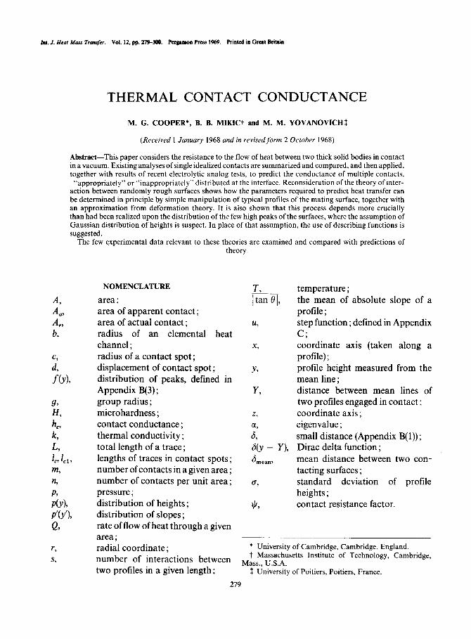
Two bodies which are in contact at nominally flat surfaces will actually touch only at a few discrete spots. Hence the exact temperature distribution is complicated and three- dimensional. An approximation, adequate for many purposes, is to define and determine a hypothetical temperature drop AT, = ( Tl - T,), as shown in Fig. 1. At a distance from the interface which is large compared with the typical spacing between conta”ctcy the temperature in each body is then taken to be:

T1 (or T,) - heat flux x distance from interface

conductivity

Provided the relative positions of the bodies do not change while the heat flux is varied, it is found that AT, is proportional to the heat flux (Q/A), and the constant of proportionality, defined by h, = (Q/A)/AT, is known as the thermal interfacial contact conductance, abbre- viated herein to contact conductance.

Thisdiscussion, in terms offlow ofheat through large plane interfaces, can reasonably be ex- tended, with obvious verbal changes, to apply to curved surfaces such as concentric cylinders with radial heat flow, provided the radius of curvature is large compared with the typical spacing between contacts.

i

T

FIG. 1. Elemental flow channel; definition of AT,.

The aim of the work is then to predict h, That is dependent upon the characteristics of the surfaces, the mechanical pressure between them, and whether there is any conducting fluid (gas or liquid) in the interstices of the interface.

Theoretical studies have generally been based on considering the flow of heat through one contact spot and adjacent solid, generally idealized as shown in Fig. 1. This idealized flow has been analyzed mathematically, as discussed in Section 2 below, but in any actual case there are many contacts of different sizes distributed across the interface. Even if we assume for the moment that the distribution of contacts is known, the pattern of flow of heat through a general distribution of contacts is extremely complicated. It is shown in Section 3 below that a reasonably accurate answer can be determined readily, provided the number and size of the contacts are known and provided they are “appropriately” distributed, in a sense discussed in Section 3. Also an approximate

THERMAL CONTACT CONDUCTANCE 281

allowance can be made in some cases for deviation of the distribution from the “appropriate” one. Zn practice, the dist~bu~on of the contacts is not generally known. Instead some information is available concerning the surfaces, in the form of detailed cross-sections, or surface roughness readings, or perhaps merely a knowledge of the method of manufacture” In Section 4 we consider how analysis of the profiles or other data can give information about number, size and distribution of contact spots. In Section S we use deformation theory, to relate the pressure between the bodies to the size and distribution of contact areas, and consider how the bodies deform under load, if for example they were not originally flat.

In Section 6 the theoretical work is synthesised to relate h, to the characteristics of the surfaces and the pressure between them, and the results are compared with results of experimental measurements of h,

2, SINGLE CONTACTS

Useful theoretical studies of the flow of heat between solid bodies have been based on considering the flow of heat through one micro- scopic contact region and adjacent solid, idealized in the form shown in Fig. 1. This problem, of flow of heat through abutting cylinders, was studied by Cetinkale and Fishenden [l] who showed that, even if the cylinders had different conductivity and heat is also conducted through the interstitial gap, there exists an isothermal plane at z = 0 (suitably subdividing the interstitial gap). The problem involving two cylinders can thus be reduced to the simpler problem of one cylinder, with in the present c;tse, temperature specified over part of the boundary and heat flux specified over the remainder. Although simpler, this problem has nevertheless defied exact analytic solution, due to the mixed boundary conditions, though an exact numerical solution has recently been reported by Clausing [2]. Some early work on the analogous electrical problem contained approximations which were only close for very small values of (c/b). Solutions

c

for larger (c/b) were obtained independently by Roess [3] and by Mikic f4], who replaced the temperature boundary c5ndition at z = 0 by a dist~bution of heat flux :

proportional to 1

(c2 - 9)) forr <c

zero fore <r -=zb,

This dist~bu~on was chosen so as to make T nearly constant at z = 0, r < c. The revised problem could be solved exactly. This has apparently not been described outside the report literature, so it is summarized in Appendix A, where it is shown to lead to

h,=uijx-$

where

and

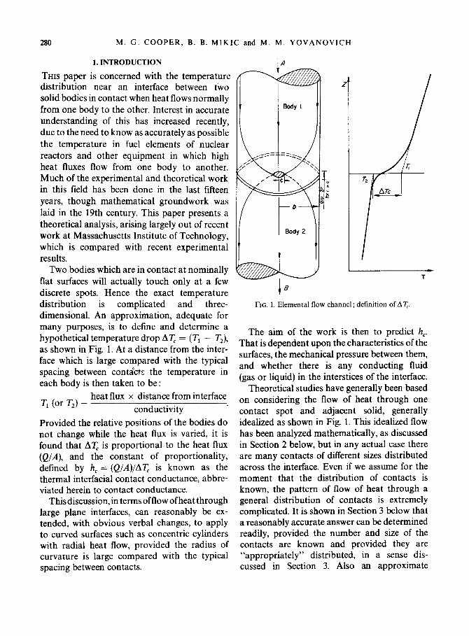
Ic/ is given by equation (A.12) or Fig. 2. The results obtained by Roess and by Mikic, though expressed in different algebraic form, agree closely for 0 K (c/Q < 0.4.

Clausing [2] reports a numerical calculation of the heat flow pattern using the true boundary conditions of zero flow at r = b and at z = 0, r > c and constant temperature at z = 0, r -z c. His result and those of Roess and Mikic are in close agreement for 0 < (c/b) c O-4 and only differ by a few percent for (c/b) = 0.6.

Clausing”s is the only calculation which aims at high accuracy for large (c/b), so the graph of $ has been continued beyond (c/b) = 0.4 by using Table 1.1 of [2] as far as that table goes, i.e. to (c/Q = 0.833. Contacts with still larger values of (c/b) will have small resistance, so the precise value of $ for larger (c/b) is of little practical importance.

As indicated in Fig. 2, various approx~atio~s can be made for tl, and the choice between them will depend on the range of (c/b) involved and the accuracy needed.

282 THERMAL CONTACT CONDUCTANCE

04

o-2

i I I I 0 01 o-2 03 04 05 0.6 07 0.8

clb

FIG. 2. Contact resistance function $.

3. MULTIPLE CONTACTS

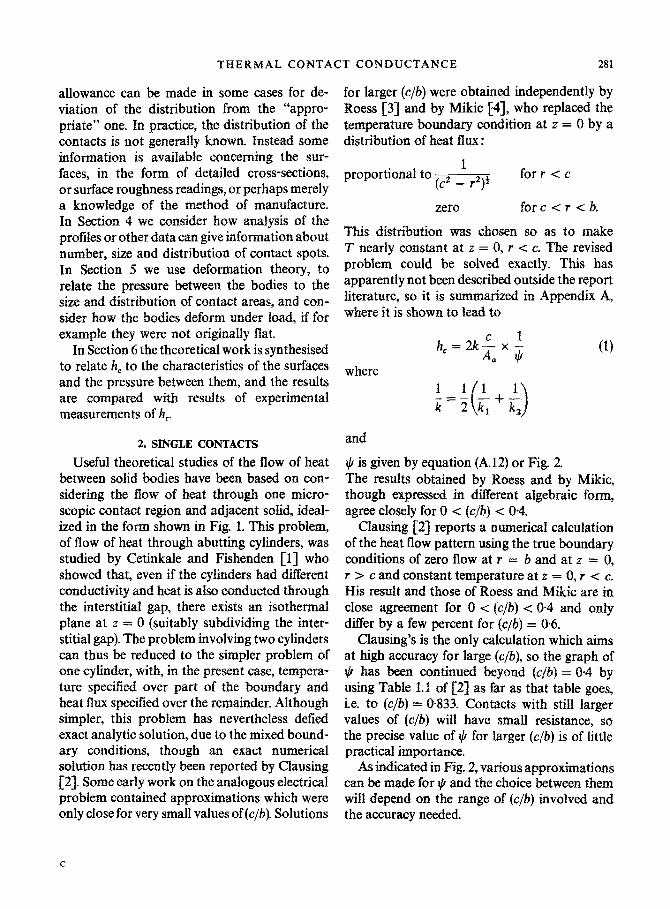
FIG. 3. General configuration and heat flow for multiple contacts at plane interface.

In the previous section the contact conductance was derived for a single circular contact spot placed centrally in a cylindrical region. The aim of this section is to extend that work towards more practical cases by considering m contacts of areas &, A,*, A,, (of equivalent radii cl, c2, . . c,) distributed over an area of apparent contact A, between abutting cylinders. It is still assumed that the interface is nearly plane, and that the heat enters and leaves the cylinders over end surfaces at great distance from the interface.

Heat flows symmetric

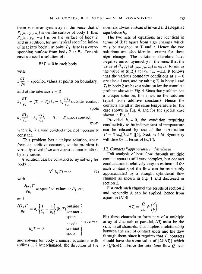
3.1 Equality of temperatures at contacts On these assumptions the local configuration Body 2

is as shown in Fig. 3, and it can be shown that all contacts must be at the same temperature, provided in each body the conductivity is independent of direction, position and tem- L

+ P2

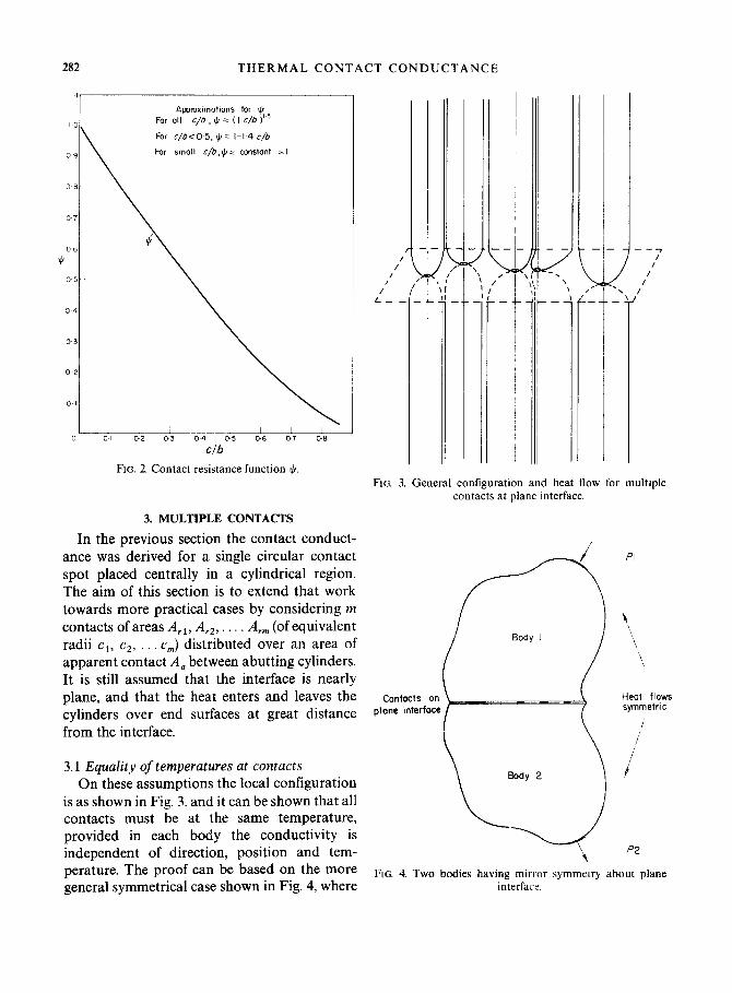
perature. The proof can be based on the more FIG. 4. TWO bodies having mirror symmetry about plane general symmetrical case shown in Fig. 4, where interface.

M. G. COOPER, B. B. MIKIC and M. M. YOVANOVICH 283

there is mirror symmetry in the sense that if P,(x,, yi, zl) is on the surface of body 1, then

P,(x,, Y11 -zJ is on the surface of body 2, and in addition, for any typical specified inflow of heat into body 1 at point P, there is a corresponding outflow from body 2 at P,. For this case we need a solution of:

with :

V’T = 0 in each body

kg = specified values at points on boundary,

and at the interface z = 0:

k, z = (TI - T2) h, = k, 2 outside contact

spots

k “T1-k 3 1 -

oz 2 dz’ T1 = Tz inside contact

spots

where I?,. is a void conductance, not necessarily constant.

This problem has a unique solution, apart from an additive constant, so the problem is virtually solved if we can construct one solution, by any means.

A solution can be constructed by solving for body 1:

with

V2(k,T) = 0 l-4

W, T) - = specified values at P,, etc.

ani

and

spots i inside r

atz=O

k,T = 0 contact spots J

and solving for body 2 similar equations with suffices 1, 2 interchanged, the direction of the

normal outward instead ofinward and a negative sign before h,,.

The two sets of equations are identical in terms of (kT) apart from sign changes which may be assigned to T and z. Hence the two solutions are also identical except for these sign changes. The solutions therefore have negative mirror symmetry in the sense that the value of (kITI) at (x,, yO, zO) is equal to minus the value of (k2T2) at (x0, y,, -zO). It follows that the various boundary conditions at z = 0 are also all met, and by taking TI in body 1 and T, in body 2 we have a solution for the complete problem shown in Fig. 4. Since that problem has a unique solution, this must be the solution (apart from additive constant). Hence the contacts are all at the same temperature for the case shown in Fig. 4, and for the special case shown in Fig. 3.

Provided h, = 0, the condition requiring conductivity to be independent of tem~rature can be relaxed by use of the substitution T’ = (l/k,)[kdT ([5], Section 1.6). Symmetry will then be in terms of (k,T’).

Full analysis of heat flow through multiple contact spots is still very complex, but contact conductance is relatively easy to estimate if for each contact spot the flow can be reasonably approximated by a straight cylindrical flow channel as shown in Fig. 1 and discussed in section 2.

For each such channel the results of section 2 and Appendix A can be applied, hence from equation (A14):

For these channels to form part of a multiple array of channels in parallel, AT, must be the same in all channels. This implies a relationship between the size of contact spots and the flow through them, since it requires that all contacts should have the same value of (2k AT,) which is {Q/(c/$)). Hence the total heat flow Q over

284 M. G. COOPER, B. B. MIKTC and M. M. YOVANOVICH

area A, must be subdivided into Q1 through contact 1, Q2 through contact 2, etc. where

hence

Q1 = Q2 = etc.

ClltcIl c2/+2

neglecting variation in Jri Alternatively, the total flow area A, can be regarded as subdivided into areas A,r , Arr2,. . . each supplying the heat flow to corresponding contacts, where

= A, 2 neglecting variation in Il/? J

(3)

If the area A, can be subdivided into these areas A,< in such a way that for all i the area Aai lies around the ith contact, then the flow at each contact spot can be reasonably approximated by Fig. 1. The contacts are then said to be “appropriately” distributed.

This is not a precise definition, but it is ~ticipated that contact conduct~ce is not greatly affected by slight deviation from “appropriate” distribution. A distribution which is sufticiently “inappropriate” to affect the conductance appreciably would appear “inappropriate” to the eye.

Since AT, is the same for all channels, and for the multiple contact region as a whole, h, for the multiple contact is the same as for any of the individual channels, namely :

= 2k 2 neglecting variation in ll/? J

Furthermore, this ratio Cc,IA, can be determined readily from protilometer traces for the mating surfaces, provided the surface rough- nesses are random (Appendix B(i)).

3.3. Contacts not “‘appropriately” distributed If the contact spots are not “appropriately”

distributed the division of heat flow and the contact conductance are greatly complicated. Intuitively it would seem that the conductance will fall. Since the conductance for the same contacts in “appropriate” distribution is readily known, we have attempted to work from that as a starting point. It would be desirable to devise a measure of the maIdist~bution which could be determined from knowledge of the layout of the contacts (or better still, from the characteristics of the mating surfaces), and then apply it to determine the decrease in conductance due to maldistribution. Some progress can be reported in this direction.

Multiple contacts. An approximation originally suggested by Holm [6] is that if two semi infinite bodies are in contact at m spots of radius c, grouped into a cluster with an envelope of radius g, then the resistance is the sum of that due to m independent contacts in parallel, each of radius c, plus that due to a single contact of radius g. This has been discussed for example by Greenwood [7]. It suggests an adaptation for multiple contacts within a cylinder, more conveniently worded in terms of tem~rature drop, that if there are m contacts of radius c, grouped into an evenly spaced cluster within radius g, in a cylinder of radius b (> g) then the interface temperature drop due to heat flow Q is equal to the sum of the temperature drop in a single contact of radius g in a cylinder of radius b with apparent heat flux Q/xb’ plus the temperature drop in a single contact of radius c in a cylinder of radius (b/Jm) with apparent heat flux Q/zb2. As Greenwood points out, these approximations depend on the partly arbitrary choice for the radius g. He calls this the Holm radius and discusses its value, finding by calculation that for contacts between semi infinite


bodies a general rule of thumb is to take 7rg2 equal to the area of an envelope lying outside each peripheral spot by a distance equal to the centre to centre separation from its nearest neighbour. For contacts between cylinders, experiments using the electrolytic analog at Cambridge University [8] and M.I.T. [9] suggest broadly that a similar definition for g is appropriate for contacts between cylinders.

Single, eccentric contact. Other experiments have been reported in which the electrolytic analog was used to study the conductance through a single circular contact spot in a cylindrical channel, when the contact is displaced from the centreline of the channel [8,10-121. The aim is to form a basis for assessing the effect of maldistribution of contacts, by regarding maldistributed contacts as lying off the centrelines of their corresponding areas A,? The method may prove to be limited in appli- cation to small displacements from “appropriate” distribution.

Considering the single eccentric contact spot as such, arguments from image theory suggest that as a small contact approaches the boundary the contact resistance would increase to approximately ,/2 times its original value, and this is borne out by experiment. Also, although most results of such tests have been expressed in terms of the fractional increase in resistance due to displacement, it is shown in [8] that, as with multiple contacts, the results could more conveniently be correlated in terms of an addition to resistance (or interfacial temperature drop) due to the displacement. For a contact displaced by distance d from the centre line of a cylinder of radius b, the increase in resistance is approximately 3(d2/bk) so the conductance is given by :

1 nb2 d2

h,=zF3bk

or, in dimensionless form

k -_=3!*+3 bh, 2 c

This is purely empirical, and the convenience lies in the surprising fact that the added resistance is independent of the contact radius c. It appears to apply for 0 < (c/b) < 05 and 0 < d < (0.85b - c) within the scatter in the experimental results, which arises from the difficulty of measuring accurately the small changes in resistance.

4. ANALYSIS OF PROFILES

In Section 3 it was shown that there is a relationship $h,/k = 2&/A, between the contact conductance in vacuum and the sum of radii of contact spots if these can be approximated to circles and are “appropriately” distributed. In section 5 it will be shown that there is a relationship AJA, = pJH between the area ratio and the ratio of apparent pressure to microhardness, on certain assumptions. The aim of this section is to link them by relating 2ZcJA, to A,/A,. We consider only surfaces which are nominally flat and have random roughness, i.e. surfaces in which the amplitude of the random roughness greatly exceeds the total amplitude of any lay or bowing across the entire surface. Initially it will be assumed that each surface is characterized by a protilometer trace. Later it will be suggested that describing functions can be defined to characterize a surface instead of using its complete profile.

4.1 Relation of profile parameters to contact and total areas

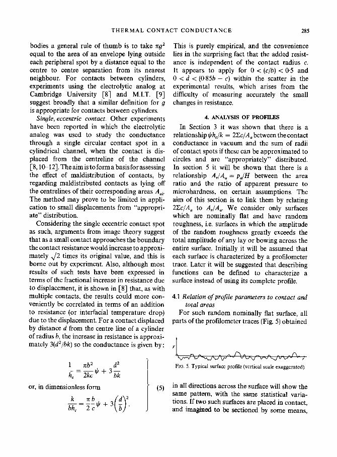
For such random nominally flat surface, all parts of the profilometer traces (Fig. 5) obtained

Y

FIG. 5. Typical surface profile (vertical scale exaggerated).

in all directions across the surface will show the same pattern, with the same statistical varia-

tions. If two such surfaces are placed in contact, and imaghred to be sectioned by some means,

286 M. G. COOPER. B. B. MIKIC and M. M. YOVANOVICH

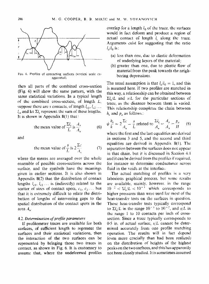
FKL 6. Profiles of contacting surfaces (vertical scale exaggerated 1.

then all parts of the combined cross-section (Fig. 6) will show the same pattern, with the same statistical variations. In a typical length of the combined cross-section, of length L, suppose there are s contacts, of length Eel, lC2.. . l,, and let X1, represent the sum of these lengths. It is shown in Appendix B( 1) that :

Cl,. 21, the mean value of L IS -i-

0

overlap for a length I, of the trace, the surfaces would in fact deform and produce a region of actual contact of length i, along the trace. Arguments exist for suggesting that the ratio

(a) less than one, due to elastic deformation of underlying layers of the material ;

(b) greater than one, due to plastic flow of material from the peak towards the neigh- boring depressions.

The usual assumption is that I$, = 1, and this is assumed here. Jf two profiles are matched in this way, a relationship can be obtained between Cl,/L and s/L for the particular sections of trace, as the distance between them is varied. This relationship completes the chain between h, and pU as fol!ows:

the mean value of i is 2 “i’ (7) i L!

where the means are averaged over the whole ensemble of possible cross-sections across the surface, and the symbols have the meanings given in earlier sections. It is also shown in Appendix B(2) that the distribution of contact lengths IfIr I,, . . is (indirectly) related to the scatter of sizes of contact spots, cl, c2.. . but that it is extremely difficult to relate the distribution of lengths of intervening gaps to the spatial distribution of the contact spots in the area A,.

where the first and the last equalities are derived in sections 3 and 5, and the second and third equalities are derived in Appendix B(1). The separation between the surfaces does not appear in that chain. but it is discussed in Section 4.4 and it can be derived from the profiles if required, for instance to determine conductance across fluid in the voids at the interface.

and

4.2. Deter~i~t~on of profile parameters If profilometer traces are available for both

surfaces, of sufficient length to represent the surfaces and their statistical variations, then the interaction of the two surfaces can be represented by bringing those two traces in contact, as shown in Fig. 6. It is customary to assume that, where the undeformed profiles

The actual matching of profiles is a very laborious graphical process. but somc results are available, mainly, however. in the range 10-2 < r-E& < 10-l which corresponds to higher pressures than were used for most of the heat-transfer tests on the surfaces in question. Those heat-transfer tests typically correspond to C&/L in the range 10e3 to lo-‘. and s/L in the range 1 to 10 contacts per inch of cross- section. Since a trace typically corresponds to 0.5 in, of actual surface, s/L cannot be determined accurately from one profile matching operation. The results will in fact depend (even more crucially than had been realized) on the distribution of heights of the highest peaks on the two surfaces, and this has apparently not been closely studied. It is sometimes assumed


that heights of a surface form a Gaussian distribution, but that distribution is often implicitly or explicitly assumed to be truncated at three or four times the standard deviation. Greenwood and Williamson [13] report finding that the distribution is nearly Gaussian for two standard deviations, but that is not enough for the present purpose. It may be very dependent on factors in the method of manufacture which have not been determined. The assumption of Gaussian distribution cannot be regarded as any more than a general guide for the distribution of these peaks.

4.3 Reduction of statistical scatter This suggests that it will be difficult to obtain

data from profile matching to give the relatign- ship required between s/L and X1,/L in the range corresponding to the experiments. How- ever, study of the probability of overlap between two Gaussian populations of standard deviation o1 if their means differ by 4.2 g1 [ = 3J(2) g,] indicates that although the probability of overlap is 10V3, the majority of the overlap arises from those parts of the individual populations lying 262.5 c1 from the mean of their populations, and the probability of such deviation from mean is lo-’ or so. As stated above, we cannot assume that the surface heights are in fact on a Gaussian distribution, but the overlap of Gaussians suggests that the peaks involved in surface interactions may not be too rare along a profile of manageable length. This suggests that the information necessary to relate s/L and ClJL in the required range may be present in the profiles, but the extraction of that information must be done more completely, giving significant reduction in the statistical scatter in the results, without further increasing the labor involved.

Recognizing at an earlier stage the need to reduce statistical scatter, Fenech [14] obtained ten readings from a single pair of profiles at the same separation by moving the profiles “sideways” (i.e. parallel to each other) to ten separate positions. This multiplied the labor

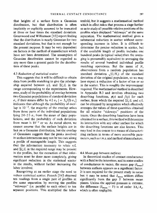
tenfold, but it suggests a mathematical method which in effect takes that process a stage further so as to study all possible relative positions of the profiles when displaced “sideways” at the same separation. The mathematical method gives a substantial reduction in scatter without corresponding increase in labor. It is difficult to determine the precise reduction in scatter, but if the available length of profile includes one hundred peaks (a typical value) then the averaging is presumably equivalent to averaging the results of several hundred individual profile matching operations. But the mean of N, observations from a random population has standard deviation J(l/N,) of the standard deviation of the original population, so we may here expect a reduction of a factor of ten or so in the scatter. This is roughly the improvement required. The mathematical method is described in Appendix B.3 and involves obtaining two describing functions, p(y) and f@) for each surface, from which the required X1,/L and s/L can be obtained by integration which effectively averages the values of these quantities obtained for all relative “sideways” positions of the traces. Once the describing functions have been obtained for a surface, this method will determine its interaction with any other surface for which the describing functions are also known. This may lead in due course to a means of characteri- zing surfaces in terms of more accessible parameters, such as r.m.s. and method ofmanufacture.

4.4 Mean gap between surfaces In theoretical studies of contact conductance

with a fluid in the interstices, and in some studies of conductance in vacua, the mean gap (6,,,,) between surfaces appears as a significant factor. It is not required for the present study in uacuo but it may be noted that a,,,, seldom differs significantly from the gap Y between mean planes. Unless the applied pressure is extreme, the difference (6,,,, - Y) is of order YAJA,,, which is often negligible.

288 M. G. COOPER. 8. 3. MTKIC and M. M. YOVANUYICH

4.5 Assumed Gaussian distribution As an alternative to the matching of actual

profiles, various theories have been developed to relate s/L and Cl& on specified assumptions about the distributions of the heights and slopes of the surfaces. Appendix C establishes the relationship, assuming the distribution of heights is Gaussian and the distribution of slopes is independent of the height. The resulting relationship is similar to that obtained by matching profiles in the range 10V2 < Cf,,JL c: IO-‘, but more information is needed to determine this applicability to the range low3 < X$/L < 10m2.

It was seen in the previous section that in order to predict contact conductance, we need a relationship between the pressure applied at the interface and the actual contact area A, or the ratio A,/A,. For normally rough surfaces un&r typica1 pressures, this ratio is very small, so the mean pressure over the actual contact area is much higher than the nominal applied pressure, and the question arises whether the material behavior is elastic or plastic. Some analyses have used Hertzian (elastic) theory, but this is not directly applicable if plastic flow occurs. If the surfaces are imagined to be moved

normally towards each other, then successive contacts are made, deformed elastically, and then may flow plastically as the nominal interference (between undeformed protIles) in- creases. Two independent studies, by Mikic [4] and by Greenwood and Williamson [ 131 suggest that even at moderate nominal pressures only very few of the contacts have s~cientfy light interference for their behavior to remain elastic. Both studies assnme that the asperities can be represented by spherical surfaces in contact, and that the heights of such asperities on the surfaces form a Gaussian distribution. Mikic employs Hertzian (elastic) analysis, to determine the stresses as a function of the interference, and deduces the interference at which elastic stresses are exceeded, so behavior be-

comes plastic. Applying this to typical surfaces of practical interest with r.m.s. a few times 10V4 in., and mean slope of profile 0.1 (as defined by equation (C5)) indicates that less than l per cent of the area in contact is in the elastic state. This conclusion is broadly supported by Green- wood and Williamson, who defined a plasticity index, p.i., and determine the fraction of contact area which remains elastic, as a function of p.i. They show that fraction fell from some 90 per cent to 50 per cent as p.i. increased from O-9 to 1.3. No means of extrapolation were given, and their work was at low pressures (15 lb/in.“), but since they report that their results were only weakly dependent on pressure, the general trend of their results suggests that, for the experiments to be reported here (for which p.i. = 2.5 or more) very little of the area in contact will remain elastic.

The matter is also affected by the history of previous foading, but for simplicity we take it that the contacts are all plastic, and we also assume that at each contact, the pressure is equal to the maximum which can be sustained by the softer of the two materials when plastically deformed. This can be related to the pressure under the indenter in a hardness indentation test, and some workers have used different values for this for different sizes of contact, because the pressure developed under an indenter depends on the size and shape of indentation However, the approximate nature of the remainder of the theory suggests that this refinement can be discarded, and we adopt the simple assumption introduced by Holm [15] that the mean pressure under contacts is H, obtained from indentation tests of size com- parable to the contacts. We will therefore use the expression :

P, 4 li=A, (9)

with H = 350,000 lb/in2 for stainless steel, and 135,@?0 lb/in.2 for aluminum.

In making this simple assumption, we are, in effect, considering the initial contact of the


two surfaces, ignoring the possible effect of previous contacts, and also ignoring possible subsequent effects due to creep, thermally induced distortition, etc.

6. RESULTS

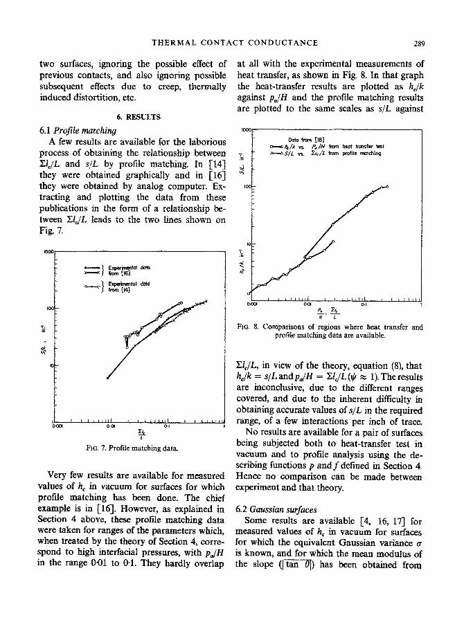
6.1 Profile matching A few results are available for the laborious

process of obtaining the relationship between C&/L. and s/L by profile matching. fn [14] they were obtained graphically and in [16] they were obtained by analog computer. Ex- tracting and plotting the data from these publications in the form of a relations~p between E&/L leads to the two lines shown on Fig 7.

FIG. 7. Profile matching data.

Very few results are available for measured values of h, in vacuum for surfaces for which profile matching has been done. The chief example is in [16]. However, as explained in Section 4 above, these profile matching data were taken for ranges of the parameters which, when treated by the theory of Section 4, correspond to high interfacial pressures, with pJH in the range 0~01 to 0.1. They hardly overlap

at all with the experimental measurements of heat transfer, as shown in Fig, 8. In that graph the heat-transfer resuhs are plotted as he/k against pJI3 and the profile matching results are plotted to the same scales as s/L against

1

FIG. 8. Comparisons of regions where heat transfer and profile matching data are availabk.

C&/L, in view of the theory, equation (8), that h,/k = s/L and p,JH = X1,/L ($ x 1). The results are inconclusive, due to the different ranges covered, and due to the inherent diffl~~ty in obtaining accurate values of s/L in the required range, of a few interactions per inch of trace.

No results are available for a pair of surfaces being subjected both to heat-transfer test in vacuum and to profile analysis using the de- scrigmg functions p andf defined in Section 4, Hence no comparison can be made between experiment and that theory.

6.2 Gaussian surfaces Some results are available [4, 16, 171 for

measured values of h, in vacuum for surfaces for which the equivalent Gaussian variance cr is known, and for which the mean modulus of the slope (ItanT) has been obtained from

290 M. G. COOPER, 8. B. MIKIC and M. M. YOVANOVICH

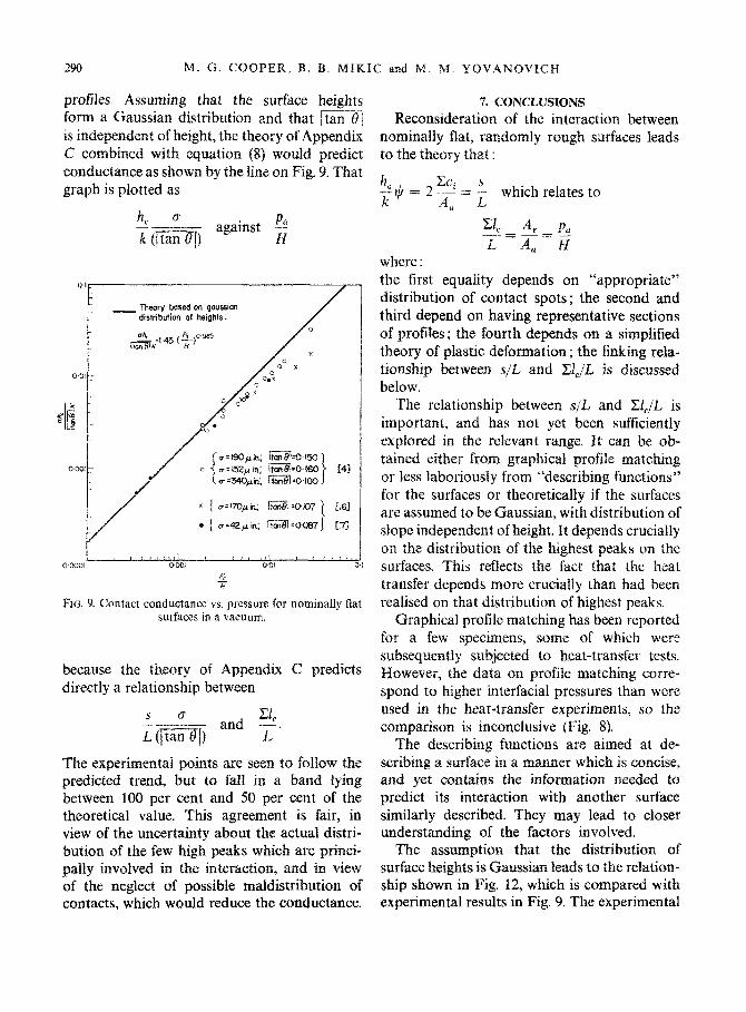
profiles. Assuming that the surface heights --- form a Gaussian distribution and that [tan 01 is independent of height, the theory of Appendix C combined with equation (8) would predict conductance as shown by the line QIZ Fig. 9. That graph is plotted as

!!L”-c_ k (W[l

against 5 N

_ Theory based on gaussian distribution of heights:

oam 0004 0.0, 0-i

e x

FIG. 9. Contact conductance vs. pressure for nominally flat surfaces in a vacuum.

because the theory of Appendix directly a relationship between

C predicts

s Q _-

L (-=-Q-/t and 5.

L

The experimental points are seen to follow the predicted trend, but to Fall in a band lying between 100 per cent and 50 per cent of the theoretical value. This agreement is fair, in view of the uncertainty about the actual distribution of the few high peaks which are princi- pally involved in the interaction, and in view of the neglect of possible maldistribution of contacts, which would reduce the conductance.

7. CONCLUSIONS

Reconsideration of the interaction between nominally flat, randomly rough surfaces leads to the theory that :

; II/ = 2 2 = 5 which relates to (1

CI A, p,, .._c - - - i A, H

where : the first equality depends on “appropriate” distribution of contact spots ; the second and third depend on having representative sections of profites ; the fourth depends on a simplified theory of plastic defo~at~o~ ; the linking relationship between s/L and SC/L is discussed below.

The relationship between s/L and X1,/L is important, and has not yet been sufficiently explored in the relevant range. It can be obtained either from graphical profiie matc~ng or less laboriously from ‘describing functions”’ for the surfaces or theoretically if the surfaces are assumed to be Gaussian, with distribution of slope independent of height. It depends crucially on the distribution of the highest peaks on the surfaces. This reflects the fact that the heat transfer depends more crucially than had been realised on that distribution of highest peaks.

Graphical profile matching has been reported for a few specimens, some of which were subs~uently subjected to heat-transfer tests. IIowever, the data on profile matching eorre- spond to higher interfacial pressures than were used in the heat-transfer experiments, so the comparison is inconclusive (Fig, 8).

The describing functions are aimed at describing a surface in a manner which is concise, and yet contains the information needed to predict its interaction with another surface similarly described. They may lead to closer understanding of the factors involved.

The assumption that the distribution of surface heights is Gaussian leads to the relationship shown in Fig. 12, which is compared with experimental results in Fig. 9. The experimental


results lie between the theoretical curve, approximated by the line:

h. Q)

and a line lower by a factor 2. Until further information is available, this can be taken to indicate the range within which the contact conductance is expected to lie. It can be determined from the,r.m.s. surface roughness and the mean slope for each of the surfaces, derived from profilometer traces.

ACKNOWLEDGEMENTS APPENDIX A The authors gratefully acknowledge the financial support

of the Unites States National Aeronautics and Space Administration, and fruitful discussions with Professors Warren M. Rohscnow and Henri Fenech.

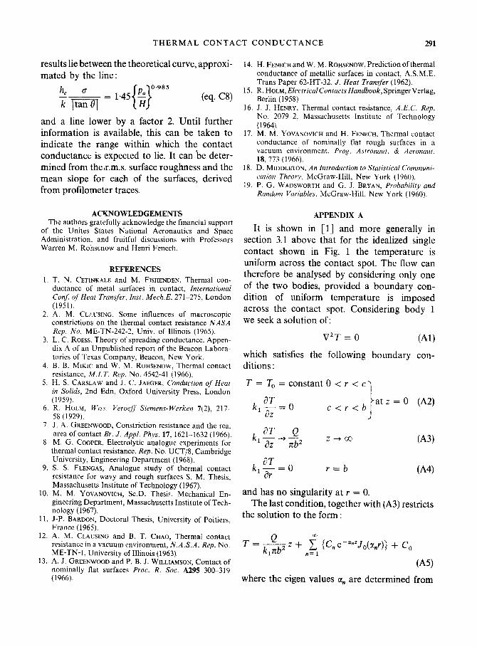
It is shown in [l] and more generally in section 3.1 above that for the idealized single contact shown in Fig. 1 the temperature is uniform across the contact spot. The flow can therefore be anaiysed by considering only one of the two bodies, provided a boundary condition of uniform temperature is imposed across the contact spot. Considering body 1 we seek a solution of:

REFERENCES

1. T. N. CETINKALE and M. FISHENDEN. Thermal conductance of metal surfaces in contact, International COI$ of Heat Transfer, Inst. Mech.E. 211-275, London (1951).

2. A. M. CLXUSING, Some influences of macroscopic constrictions on the thermal contact resistance NASA Rep. No. ME-TN-242-2, Univ. of Illinois (1965).

3. L. C. ROESS, Theory of spreading conductance. Appen- dix A of an Unpublished report of the Beacon Labora- tories of Texas Company, Beacon. New York.

4. B. B. MIKIC and W.. MI ROHSENOW, Thermal contact resistance. M.I.T. Reo. No. 4542-41 (1966).

5. H. S. CARSLAW and i. C. JAEGER, Conduction of Heat in Solids, 2nd Edn, Oxford University Press, London (1959).

6. R. HOLIM, U’KS. Veroejj’ Siemens-Werken 7(2), 217- 5X (1929).

7. J. A. GREENWOOD, Constriction resistance and the real area of contact Br. J. Appl. Phys. 17, 1621-1632 (1966).

8. M. G. COOPER, Electrolytic analogue experiments for thermal contact resistance. Rep. No. UCT/S, Cambridge University, Engineering Department (1968).

9. S. S. FLENGAS, Analogue study of thermal contact resistance for wavy and rough surfaces S. M. Thesis, Massachusetts Institute of Technology (1967).

10. M. M. YOVANOVICH, Sc.D. Thesis. Mechanical En- gineering Department, Massachusetts Institute of Tech- nology (1967).

11. J-P. BARDON, Doctoral Thesis, University of Poitiers, France (1965).

12. A. M. CLAUSING and B. T. CHAO, Thermal contact resistance in a vacuum environment, N.A.S.A. Rep. No. ME-TN-l, University of Illinois (1963).

13. A. J. GREENWOOD and P. B. J. WILLIAMSON, Contact of nominally flat surfaces Proc. R. Sot. A295 300-319 (1966).

14.

15.

16.

17.

18.

:9.

H. FENECH and W. M. ROHSENOW, Prediction of thermal conductance of metallic surfaces in contact, A.S.M.E. Trans Paper 62-HT-32, J. Heat Transfer (1962). R. HOLM, Electrical Contacts Handbook, Springer Verlag, Berlin (1958). J. J. HENRY, Thermal contact resistance, A.E.C. Rep. No. 2079-2. Massachusetts Institute of Technology (1964) M. M. YOVANOVICH and H. FENECH, Thermal contact conductance of nominally flat rough surfaces in a vacuum environment. Prog. Astronaut. & Aeronaut. 18, 773 (1966). D. MIDDLETON, An Introduction to Statistical Communi- cution Theory, McGraw-Hill, New York (1960). P. G. WADSWORTH and G. J. BRYAN, Probabilit~l and Random Variables, McGraw-Hill, New York (1960).

v27’ = 0 (Al)

which satisfies the following boundary conditions :

T = To = constant 0 < Y < c 1

k %() atz = 0 (A2)

1 i?z C<Y<h

k!? 2

1 aZ -+ xb2 Z-+00

k%(J 1 ay

r=b (A4)

and has no singularity at Y = 0. The last condition, together with (A3) restricts

the solution to the form :

T= & z + f {C, e-a+Jo(a,r)} + Co 1 n=1

(A5)

where the eigen values an are determined from


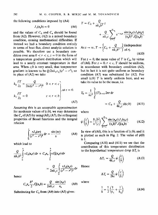
the following conditions imposed by (A4)

J,@“b) = 0 (A6)

and the values of C, and C, should be found from (A2). However, (A2) is a mixed boundary condition, causing mathematical difficulties. If instead we had a boundary condition entirely in terms of heat flux, direct analytic solution is possible. We therefore use a boundary condition over area 0 < I < c, z = 0 in the form of a temperature gradient distribution which will lead to a nearly constant temperature in that area. When c/b is very small, that temperature gradient is known to be Q/27rklcJ(c2 - r’), so in place of (A2) we take

kT= Q l az 2nc(c2 - r2)f

O<r<c 1 k !Lo l az !

at z = 0.

c<r<b

tA7)

Assuming this is an acceptable approximation for moderate values of (c/b), we may determine the C,, of (A5) by using (A6), (A7), the orthogonal properties of Bessel functions and the integral relation

c

s rJo@) sin (ac)

(c2 - r2)* dr = - (‘48)

CI 0

which lead to

Q b b

nk,b2 s rJ,(a,r) dr + C,CX, s

rJi(a,,r) dr

0 0

Q ’ s rJohd dr

= Z&i (c2 - r2)*

hence 0

e _ a,z sin (CL,C) Jo&v)

(a,b)2 J&=,4 . n=1

For z = 0, the mean value of T is Co, by virtue of (A6). For z = 0, r < c, T should be uniform, in accordance with boundary condition (A2), but in fact it is not quite uniform as boundary condition (A7) was substituted for (A2). For small (c/b) T is nearly uniform here, and we take its value to be the mean, i.e.

c

TO = -$ (Tbzo 2nrdr s 0

= co + $ W/b) (All)

where

In view of (A6), this is a function of (c/b), and it is plotted as such in Fig. 2 The value of t@(O) is 1.

Comparing (AlO) and {Ail) we see that the contribution of this temperature distribution to the hypothetical temperature drop AT, is

AT, =

Hence

Ax=& f 0

Q sin (oI,c) C,p,, p J$(qb) = - -

2nk,c a,, (A9)

where

Substituting for C, from (A9) into (A5) gives :

W3)

6414)


and

h _ @ _ 2kc e

AT, nb2$(c/b) (A15)

APPENDIX B(1)

Three Geometrical Propositions

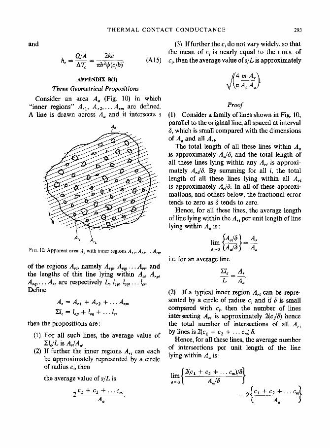
Consider an area A, (Fig. 10) in which “inner regions” & Ar2,. . . A,.,,, are defined. A line is drawn across A, and it intersects s

‘2

FIG. 10. Apparent area A, with inner regions A,,. A,,, A,,

of the regions Ariv namely Alp, Alq,. . . A,, and the lengths of this line lying within A,, Alp, A rq, . . * A,, are respectively L, lep, leq, . . . I,,.. Define

A, = A,, + A,, + . . . A,,,,

El, = I,, + I,, + . . . 1,,

then the propositions are :

(1) For all such lines, the average value of UC/L is A,/A,

(2) If further the inner regions A,i can each be approximately represented by a circle of radius Cg then

the average value of s/L is

2 Cl + c2 + . . . c,

4 ’

(3) If further the ci do not vary widely, so that the mean of ci is nearly equal to the r.m.s. of Ci, then the average value of s/L is approximately

Proof

(1) Consider a family of lines shown in Fig. 10, parallel to the original line, all spaced at interval 6, which is small compared with the dimensions of A, and all Arti

The total length of all these lines within A, is approximately Add, and the total length of all these lines lying within any A,i is approximately A&3. By summing for all i, the total length of all these lines lying within all A,i is approximately A,/& In all of these approximations, and others below, the fractional error tends to zero as 6 tends to zero.

Hence, for all these lines, the average length of line lying within the A,i per unit length of line lying within A, is :

i.e. for an average line

3 _ 4 - -. L A,

(2) If a typical inner region A,i can be represented by a circle of radius Ci and if 6 is small compared with ci, then the number of lines intersecting Ari is approximately 2(c,/6) hence the total number of intersections of all Ari by lines is 2(c1 + c2 + . . . c,,,) 6.

Hence, for all these lines, the average number of intersections per unit length of the line lying within A, is :

lim 2(c, + c2 + . . . c&3

a=0 I 4~ I 2 I

Cl + c2 + . . . c, = 1 -I A, J


i.e. for an average line The probability that the line also produces a

s 2

r

Cl + c2 + c, contact length lying between 1 and I + dl in

-_= L A, 1.

that circle is

Id1 (3) If mean ci is approximately equal to r.m.s. ci. then

;NP(c)dc __ 2c(4c2 - 12)o.s

NP(c) dc 1 dl = 2~(49 _ 12)o.s (0 < 1 < 2c)

so the probability of a random line across the circle of radius R producing a contact length lying between 1 and 1 + dl is:

2m =-

A,

Hence this gives the distribution of contact lengths along a profile which is an (inaccurately)

APPENDIX B(2) observed quantity. To find P(c) from it would 1. Distribution of Sizes of Contact Spots probably be feasible using some iterative pro-

It would be of interest to know the distribution cedure on a computer. Alternatively, by approxi-

of sizes of contact spots at an interface, and it mating the function

may be asked whether this can be deduced from 1 dl the distribution of contact lengths 1, along a typical length of matched profiles. If all contact

2c(4c2 - P)o.5

spots were circles of the same radius c, then to a straight line, P(c) can be deduced approxi-

not all contact lengths for lines cutting the mately from the observed distribution of contact

circles would bc of the same length. The average lengths. No satisfactory straight line approxi-

length would be (7r/2) c and the distribution can mation is possible, though one might be used as

be shown to be such that the probability of a a starting point for computer solution.

contact length lying between 1 and I + dl is: The problem is therefore not simple, and the

1 dl accuracy of any result will be limited by the

2c(4c2 - /2)“‘5 for 0 < 1 < 2c statistical scatter arising from obtaining the

distribution of contact lengths from some given zero for 2c < 1. finite length of matched profiles.

If there are N contacts, lying in a circle of radius R and they are not all of the same size, 2. Spatial Distribution of Contact Spots but have probability distribution P(c), so that NP(c) dc is the number of contacts having It would also be of interest to determine

radius between c and c + dc, then the probability whether contacts are distributed “appropriately”

that a random line across the area of radius R across the region, or whether some are grouped

will cut a contact of radius between c and closely together. If there are n equal contacts

c + dc is per unit area, uniformly distributed, then the area surrounding each contact is l/n and each

f NP (c) dc. contact will be at a distance of order 21 Jn from its neighbors. But the average length of gap

CE4,

[s

P(c) dc

(4c2 - 12)“” 1 Nl dl ~_ 2R ’

c=1/2


along a pair of matched profiles is nearly equal to the pitch of the contacts, which is L/S, which is ~~~ro~~t~~~

Hence, to detect crowding of contacts we need to study the d~str~bntion of gap lengths frr s cien~ de&if to ~e~e~~~e W&&XX there are many gaps oF length < ~~~~ which is

A J( > n--L Ail

times ihe mean gap lenge. This involves dose study of the %@ of a d~s~~~~~o~, far from its mean. Such a study requires much ~nfo~at~~~ if it is to be at all accurate. Therefore, it seems impracticable to obtain information a’trout

horizontally with vertical distance Y between the datnm planes (Fig. S), the quantities normahy ~~t~~ed from profile rnat~~~ by meas~~ng atong the profifes are:

El, L and i

res~e~t~~~~~ &G lotal con&& length and the number of ~o~t~~t~ divided in each case by the length of the trace. ff the profiles are d~sp~~~ed horizontally while keeping Y the same, these quantities will vary statistica.lly, and it is desirable to obtairr the mean of such variations,

These means cam be obtamed if two describing f~~t~~~s &$ and f(y) are known for each surface, defined as functions of J’, the distance from a datum plane (conveniently the mean plane) so that :

p(y)dy = length ~3 trace lying ~tween heights p, 3~ + dy

total length of trace

number of peaks with tip height between y, y + dy fW4~ - - tatal length of trace

“-7

m s p(t)dt = length of trace lying above height v

total. 1ecgt.h of trace .,“._“A

Y

provided in the case of Y(J) that y exceeds the height of the highest ““vaIley’” y,.

gr~nFjng of caxltacts from study of profifes of smfa~es which are nearly random If the prof%s show evidence of strong waviness dne to machining marks, then maldistribution of contacts may be deduced from that alone.

If the profiles are imagined to be placed

The f~~~o~s ps f and y am only required for those vah~es of p for which ~~fer~~~~on with the opposing surface is possible (ty~~~a~l~ y1 > 1.50,).

If the profile is available in graphical or andog form then the integrals are similar to the quantities ~~~o~~y obt~~ by &e tecfl- niqnes of ~~~~ or analog profile ma~h~g. Those techniques can be used here, though here the process is simpler as it does not involve

296 M. G. COOPER, B. 8. MIKIC and h4. M. YOVANOWCH

recognition of contacts, so it lends itself more readily to automatic processing, perhaps using optical projection.

If the profile is available in digital form, it may be simpler to obtain the functions p and f directly.

Given these describing functions pl(yl),fi(yl) for surface 1, and pz(yz), fi(_vz) for surface 2, then the following relationships apply, as proved in section B(3), 2 below:

mean value of $

mean value oft

where, on the left of these equations the mean has considered all possible relative horizontal positions of the two profiles at separation Y, and on the right hand the double integral can be evaluated by digital computer. If the program is arranged to integrate along lines y1 + y, = constant, then it can produce successively answers for successively increasing values of Y

The first equation is exact. The second equation contains a factor C1 which has the value O-7 if the tips of the peaks are assumed to be spherical.

Modification may be needed if

(~5~ + yZmaX) > Y or (yImax + YD) > Y.

Other quantities can also be detrained in terms of these describing functions p and f

The mean value of the modulus of the reciprocal of the slope of the profile at height y is :

mean p&j ( i &Yl =?y@

if y > _yV

where this mean is a simple arithmetic average

for all of the points on the profile where distance from the mean plane is y_

2, broom U~~~l~~~~~~~~~ Stated in 43).1

Consider those parts of profile 1 which lie at distance < y, + dy,, > y, from the mean plane In length L of trace the total length of such parts of profile is

Consider the profile of surface 2 as traversing horizontally past these parts of surface 1. The fraction of the traverse during which these parts of surface 1 are in contact with surface 2 is

pt= co

yJ~_-y,) PJ”vJdy2*

Integrating for all yl, the mean length in contact during the traverse is

tYl+YzPy

Consider those peaks of profile 1 which lie at distance < yi + dy, > y, from the mean piane. In length L of trace the total number of such peaks is

l;f,cVJ dy,.

Consider the profile of surface 2 as traversing horizontally past these peaks of surface 1. The fraction of the traverse during which these peaks of surface I are in contact with surface 2 is

3?4==J

s ~z(Yz) dy,,

yz=‘( -Yd

Integrating for all yr, the mean number of peaks of surface 1 which are in contact with surface 2 during the traverse is


which is

L (yI it)> y ficVJ PA) dY, dY,

where “peak” here refers strictly to the topmost point of the asperity.

Neither this quantity nor the symmetrical quantity

L(Y1+!,>Y PAYIMYZ) dy, dy,

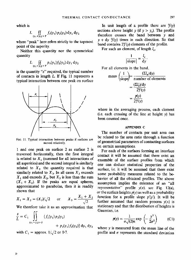
is the quantity ‘3” required, the typical number of contacts in length L. If Fig. 11 represents a typical interaction between one peak on surface

/

/

FIG. 11. Typical interaction between peaks if s&faces are moved relatively.

1 and one peak on surface 2 as surface 2 is traversed horizontally, then the first integral is related to X, (summed for all interactions of all asperities) and the second integral is similarly related to X,. the quantity required is that similarly related to X,. In all cases X, exceeds X, and exceeds X,, but X, is less than the sum (X, + X,). If the peaks are equal spheres, approximated to parabolas, then it is readily shown that

X, = X, = (X,)/J2 or X, = Xl;2X2

We therefore take it as an approximation that

S -_= L Cl ss u-ICYI) P2012)

(Yl+Yz)‘Y

+ PI(YIV~(Y~))~~~ dy,

with C, = approx. l/J2 or 0.7.

In unit length of a profile there are y(y) sections above height y (if y > y,). The profile therefore crosses the band between y and y + dy y(y) times in each direction. So that band contains 2y(y) elements of the profile.

For such an element, of length l,,

For all elements in the band,

1

( >

(%/dY) mean - =

slope number of elements

(%)/dY =--- 2!f(Y)

P(Y) =m

where in the averaging process, each element (i.e. each crossing of the line at height y) has been counted once.

APPENDIX C

The number of contacts per unit area can be related to the area ratio through a function of geometrical parameters of contacting surfaces on certain assumptions.

For each of the surfaces forming an interface contact it will be assumed that there exist an ensemble of the surface profiles from which one can deduce statistical properties of the surface, i.e. it will be assumed that there exist some probability measures related to the behavior of all the obtained profiles. The above assumption implies the existence of an “all representative” profile y(x), see Fig. 12(a), or the surface heights p(y) as well as a probability function for a profile slope p’(j). It will be further assumed that random process y(x) is stationary and that the distribution of heights is Gaussian, i.e.

p(y)-.L _2$ oJ(2)rc exp ( >

(Cl)

where y is measured from the mean line of the profile and g represents the standard deviation

D

298 M. G. COOPER, B. B. MIKIC and M. M. YOVANOVICH

of the surface heights specified by L +SX

1 c2, limL y2dx= Y%(Y) dy.

L'CC s s 0 -0D

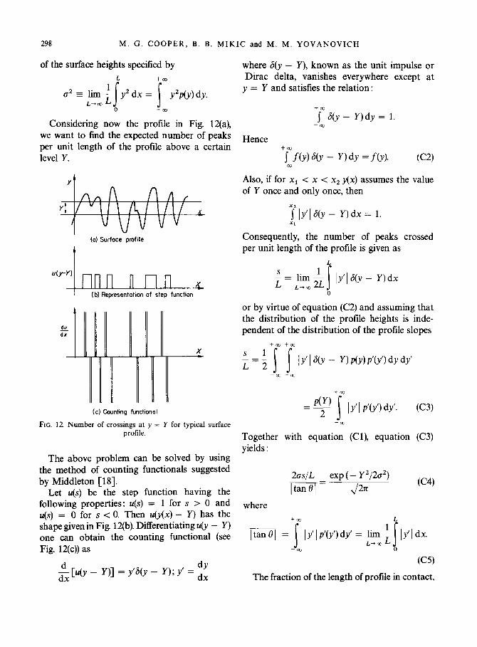
Considering now the profile in Fig 12(a), we want to find the expected number of peaks per unit length of the profile above a certain level Y.

where S(y - Y), known as the unit impulse or Dirac delta, vanishes everywhere except at

y = Y and satisfies the relation :

+[S(y - Y)dy = 1. --oo

Hence

Y[~(Y) &y - Y) dy = f(y). (C2)

Also, if for x1 < x < x2 y(x) assumes the value of Y once and only once, then

$y’16(y - Y)dx= 1.

(a) Surface pmfile Consequently, the number of peaks crossed

t per unit length of the profile is given as

dy-Y)

I-In nnn xl_ (b) Representation of step function

(c) Counting functional

FIG. 12 Number of crossings at y = Y for typical surface profile.

The above problem can be solved by using the method of counting functionals suggested by Middleton [18].

Let u(s) be the step function having the following properties: u(s) = 1 for s > 0 and u(s) = 0 for s < 0. Then z&(x) - Y) has the shape given in Fig 12(b). Differentiating ~0, - Y) one can obtain the counting functional (see Fig. 12(c)) as

&y - Y)] = y’qy - Y); y’ = 2

L

S 1 -=,‘“Eo Iy’IiS(y- Y)dx L s

or by virtue of equation (C2) and assuming that the distribution of the profile heights is independent of the distribution of the profile slopes

tm tm s 1

x=2 IS I Y’ I S(Y - Y) P(Y) P’(Y’) dy dy’

--io -cc

P(Y) +m = - 2 s

1 y’ 1 p’(y’) dy’. (C3)

-m

Together with equation (Cl), equation (C3) yields :

2aslL exp ( - Y ‘/2a2)

F[= J2n (C4)

where

(C5)

The fraction of the length of profile in contact,


X1,/L can be obtained. From the definition of

P(Y): cc

CL -= tiy)dy L s

((3)

Y

which can be obtained from tables, since p(j~) is given by (Cl).

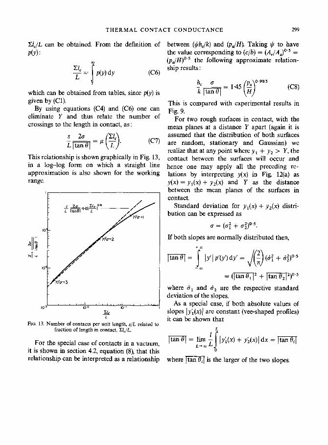
By using equations (C4) and (C6) one can eliminate Y and thus relate the number of crossings to the length in contact, as:

s 20 CL --= L]tan[ PT. 0

(C7)

This relationship is shown graphically in Fig 13, in a log-log form on which a straight line approximation is also shown for the working range.

FIG. 13. Number of contacts per unit length, s/L related to fraction of length in contact, Z&/L.

For the special case of contacts in a vacuum, it is shown in section 4.2, equation (8), that this relationship can be interpreted as a relationship

between (t+bhJk) and (p,,/H). Taking Ic/ to have the value corresponding to (c/b) = @,/A,)“” = (P,JH)“~ th e 0 owing approximate relation- f 11 ship results :

h CJ -z- = I.45 $$ 0.985

kvf 0 (W

This is compared with experimental results in Fig. 9.

For two rough surfaces in contact, with the mean planes at a distance Y apart (again it is assumed that the distribution of both surfaces are random, stationary and Gaussian) we realize that at any point where y, + y, > Y, the contact between the surfaces will occur and hence one may apply all the preceding relations by interpreting y(x) in Fig 12(a) as y(x) = yi(x) + yz(x) and Y as the distance between the mean planes of the surfaces in contact.

Standard deviation for yi(x) + yz(x) distribution can be expressed as

0 = (0: + cr$)“?

If both slopes are normally distributed then,

Itan/ = r 1 y’ 1 p’(y’) dy’ = d(i) (6: + ti;)“‘5

-m

= (1~8, + Tizii7q)O.J

where til and c?~ are the respective standard deviation of the slopes.

As a special case, if both absolute values of slopes (y;(x)/ are constant (vee-shaped profiles) it can be shown that

L

m = lim ; 1 y;(x) + y;(x) 1 dx = )q L-+.X s

0

where )[ is the larger of the two slopes.

300 THERMAL CONTACT CONDUCTANCE

R&urn&On examine darts cet article la resistance au flux de chaleur entre deux corps pleins tpais en contact darts le vide. L’analyse existante des contacts simples ideali& est r&sum&e et comparee, puis appliqued, en m&me temps que des resultats d’essais recents d’analogie tlectrolytique, afin de p&dire la conductance de contacts multiples, distribute a l’interface d’une facon “appropriee” ou “inappropriee”. La reconsideration de la theorie de l’interaction entre des surfaces avec une rugosite distribuee au hasard montre comment les parametres necessaires pour p&dire le transport de chaleur peuvent &tre determines en principe par une manipulation simple de profils typiques de la surface associte, en m&me temps qu’une approximation a partir de la theorie de la deformation. On montre aussi que ce processus depend, plus crucialement que celui qui avait Cte rbalise, de la distribution des quelques grands pits des surfaces, oh l’hypothese d’une distribution gaussienne des hauteurs est suspecte. A la place de cette hypothese, l’usage de fonctions descriptives est suggere.

Les quelques r&hats experimentaux se rapportant a ces theories sont examines et compares avec les previsions theoriques.

Zusammenfassung-Die Arbeit befasst sich mit dem Widerstand, den zwei dicke feste Korper, die sich im Vakuum beriihren, einem Wiirmestrom entgegensetzen. Die bestehenden Analysen tiber einzelne idealisi- erte Kontakte wurden zusammengestellt und dann-zusammen mit Ergebnissen kiirzlich durchgeftihrter Analogieversuche im elektrolytischen Trog- zur Bestimmung der Leitfahigkeit einer Vielzahl von Kontakten mit “ordentlicher” oder “unordentlicher” Verteilung tiber die Kontaktflache herangezogen. Unter Verwendung der Theorie der Zwischenwirkung zwischen willktirlich rauhen Oberfl&chen wird gezeigt, wie die zur Berechnung des Wlrmetransportes erforderlichen Parameter durch prinzipiell einfache Behandlung mit typischen Profilen der beriihrenden Oberflache zusammen mit einer Niiherung fur die Deformationstheorie bestimmt werden konnen. Es wird such gezeigt, dass dieser Prozess weit starker als angenommen auf der Verteilung der wenigen grossen Spitzen an den Oberflachen beruht, woftir die Annahme einer Gauss’schen Verteilung der Spitzen zweifelhaft ist. Anstelle jener Annahmen werden beschreibende Funktionen vorgeschlagen.

Die wenigen experimentellen Werte ftir diese Theorien wurden geprtift und mit theoretischen Ergebnissen verglichen.

AHnoTapu?-B AaHHO& CTaTbe paCCMaTpHBaeTCH COIIpOTRBJIeHRe TeIIJIOBOrO IIOTOKa MeHcRy

AByMH TOJICTbIMHTBep~bIMHTeJIaMLI,HaXO~RIL(RMMCR B KOHTaHTe,B BaKyyMe. AJIR OIIpeaeJIe-

HHH TeIIJIOIIpOBO~HOCTH MHOrO'JHCJleHHbIX KOHTBKTOB, paCItOJIOH(eHHblX Ha rpaHAqe pa3neJIa

B OnpeAeJIeHHOM IIOpfiaKe H IIpOII3BOJIbH0, MCIIOJIb3yKlTCH He,IQaBHO IIOJIyYeHHbIe WCIIepH-

MeHTaJIbHbIe AaHHbIe II0 FNIeKTpOJIHTWeCKOMy aHaJIOry, a TaKwe pe3ynbTaTbI aHanI43a

eRI%HWIHbIX. IlAeaJIbHbIX KOHTBKTOB. TeopvrH B3aHMORetiCTBUFl XaOTHqHO paCnOJIOmeHHbIX

ruepoxoBaTbIx noBepxHocTei2 noKa3bIBaeT, KaK, 3HaR HeO6xOHHMkJe napaMeTpbI, MOWHO

OIIpe~enllTb TeIIJIOO6MeH C IIOMOUbIO IIpOCTOfi MaHHIIyJIXIJHK 06bWHbIx IIpO@UIefi IIOBepX-

HOCTH,~T~K?K~ c IIOMO~bH) annpoKcnMa~am ~3 Teopnll ~e$OpMaIJHH.TaKxte nOKa3aH0,YTO

3TOTIIpOI(eCCCy~eCTBeHHO 3aBIlCIIT OTpaCIIpeAeJIeHLlR HeCKOJIbKLIX 6Onbmax IIKKOB IIOBepX-

HOCTet,HOrRa~OIIyIJeH,'Ie rayCCa AJIH 3TI4X BbICOT 0 paCIIpe~eJIeHHI4 EaBJIeHHH COMHMTeJIbHO.

BMecTo aTor AonyweHLin npeanaraeTcH wznonb30BaTb $y~Kqw pacnpegeneHsfH.

klCCJIe~yIOTCSl 3KCIIepI4MeHTaJIbHbIe AaHHbIe I4 CpaBHRBaIOTCH C paWeTaMM TeOpMH.

Documents

THERMAL CONTACT CONDUCTANCE - … · THERMAL CONTACT CONDUCTANCE ... Abstract-This paper considers the resistance to the flow of heat between two thick solid bodies in contact