KTH Electrical Engineering 

Theory of transformation optics and invisibility cloak design

 

 

 

 

 

 

PU ZHANG

 

 

 

 

 

 

 

 

 

                     

 

Doctoral Thesis in Electromagnetic Theory Stockholm, Sweden 2011

 

TRITA-EE 2011:028 Elektroteknisk teori och konstruktion ISSN 1653-5146 Teknikringen 33 ISRN KTH/EE--11/028--SE SE-100 44 Stockholm ISBN 978-91-7415-947-9 Sweden Akademisk avhandling som med tillstånd av Kungl Tekniska högskolan framlägges till offentlig granskning för avläggande av teknologie doktorsexamen fredag den 6 Maj 2011, klockan 10:00 i sal F3, Lindstedtsvägen 26, Kungl Tekniska högskolan, Stockholm. © Pu Zhang, March 2011. Tryck: Universitetsservice US AB

III 

Abstract Research on metamaterials has been growing ever since the first experimental realization of a

double negative medium. The theory of transformation optics offers a perfect tool to exploit the

vast possibilities of the constitutive parameters of metamaterials. A lot of fascinating optical

devices have been identified, especially invisibility cloaks. The aim of this thesis is to contribute to

the development of the basic theory of transformation optics, and use it to design invisibility cloaks

for various applications.

Background and the theory of transformation optics are introduced first. Formulas of

transformed material parameters and transformed fields are thoroughly derived and detailed

explanations are provided, so that the working knowledge of transformation optics can be acquired

with minimal prerequisite mathematics. A proof of the form invariance of full Maxwell’s equations

with sources is presented. Design procedure is then demonstrated by creating perfect invisibility

cloaks. The introduction to the basic theory is followed by discussions of our published works.

In the first application, a method of designing two-dimensional simplified cloaks of complex

shapes is proposed to remove the singularity occurring in perfect cloaks. This intuitive and rather

simple method is the first way to design two-dimensional simplified cloaks of shapes other than

circular. Elliptical and bowtie shaped simplified cloaks are presented to verify the effectiveness of

the method. Substantial scattering reduction is observed in both cases.

Due to practical considerations, transformations continuous in the whole space must be the

identity operation outside a certain volume, and thus they can only manipulate fields locally.

Discontinuous transformations are naturally considered to break this limitation. We study the

possible reflection from such a transformed medium due to a discontinuous transformation by

introducing a new concept: inverse transformation optics. In this way, the reflection falls into the

framework of transformation optics as well. Necessary and sufficient condition for no reflection is

then derived as a special case.

Unlike the invisibility realized by perfect cloaks, cloaking an object over a dielectric

half-space has advantages in some particular applications. Starting from a perfect cloak, a

half-space cloak is designed to achieve the invisibility in an air half-space over a dielectric ground.

In our design, two matching strips embedded in the dielectric ground are used to induce proper

reflection in the air half-space, so that the reflected field is the same as that from the bare

dielectric ground.

Cloaks obtained from singular transformations and even simplified models all have null

principal values in their material parameters, making invisibility inherently a very narrowband

effect. In contrast, a carpet cloak designed by only coordinate deformation does not have the

narrowband limitation, and therefore can perform well in a broad spectrum. The invisibility

accomplished by the carpet cloak is only with respect to EM waves in a half-space bounded by a

perfect electric conductor, similar to the previous half-space cloak. In this part, we extend the

IV 

original version of the carpet cloak to a general dielectric ground.

Key words: Transformation optics, Maxwell’s equations, invisibility cloak, half-space cloak, simplified

cloak, inverse transformation optics, carpet cloak.

V 

Acknowledgments 

The dissertation is the conclusion of the whole Ph.D. study. Accordingly, I would like to take this

chance to extend my gratitude to all people who helped me during the six years, both with the

work and my life. The thesis wouldn’t be accomplished without their help. However, it is not

possible to include all of them in this short acknowledgement. Hope those people I missed out in

the following can accept my sincere appreciation at this moment.

At first, I would like to express my gratitude to my supervisor Prof. Sailing He for his

excellent guidance (not just scientific). His advice and encouragement have been of vital

importance during my research work.

I also would like to thank Prof. Martin Norgren for his nice co-supervision, the

electrodynamics course he provided, and the comments on and revision of this thesis.

Another person I’m much indebted to is Prof. Lars Jonsson. Academically, I learned a lot

from the electromagnetic wave propagation course and several discussions with him. In other

aspects, he gave me much advice on how to do a Ph.D. I also want to thank him for reading my

thesis and the suggestions on revision.

Thanks then goes to Dr. Yi Jin. The valuable discussions with him, his advice, and

experienced instruction helped greatly with my research work at the beginning stage.

I also thank Prof. Jianqi Shen for his instruction on my early work on electromagnetically induced transparency. His broad range of knowledge in theoretical physics introduced to me a wider view of optics.

In the Department of Electromagnetic Engineering, there are still more people I want to thank.

I took the courses of electromagnetic compatibility and applied antenna theory given by Peter

Fuks and Anders Ellgardt. When doing the labs and projects, I got much instruction from them.

Our financial administrator Ms. Carin Norberg is the one I turn to help with administration. Her

effort makes the work and life much easier. I also thank Peter Lönn for his continuous support in

maintaining computers and software. Prof. Rajeev Thottappillil, the head of the department,

deserves special thanks for a friendly atmosphere. The time spent together with Xiaolei Wang,

Yalin Huang, Helin Zhou, Kelin Jia, Fei Xiao, Jialu Cheng, Xiaohu Zhang, Toshifumi Moriyama,

Andres Alayon Glazunov, Venkatesulu Bandapalle, and Siti Jainal is going to become beautiful

memories.

During the stay in Sweden, I’m lucky to have the company of my friends: Haiyan Qin, Hui Li,

Shuo Zhang, Mei Fang, Xuan Li, Xin Hu, Zhangwei Yu, Geng Yang, Shuai Zhang, Yongbo Tang,

Zhechao Wang, Rui Hu, Yiting Chen, Kai Fu, Yukun Hu, Yuntian Chen, Salman Naeem Khan,

Sanshui Xiao, Chenji Gu and more. Thanks are due to my friends and colleagues in China as well.

I acknowledge China Scholarship Council (CSC) for the financial support of my study at

KTH. Last but of course not least, I thank my parents for their love and support all the time.

VI 

Pu Zhang Stockholm, March 2011

VII 

Table of the Contents Abstract ............................................................................................................................................III Acknowledgments............................................................................................................................ V List of publications ...........................................................................................................................IX Acronyms..........................................................................................................................................XI 1. Introduction ..................................................................................................................................1

1.1 Background .........................................................................................................................1 1.2 Thesis Outline......................................................................................................................3 References.................................................................................................................................4

2. Theory of Transformation Optics ..................................................................................................9 2.1 Elements of Coordinate Transformation .............................................................................9 2.2 The Form Invariance of Maxwell’s Equations....................................................................13 2.3 Transformation Optics with Orthogonal Coordinates .......................................................20 2.4 Spherical and Cylindrical Invisibility Cloaks.......................................................................22 References...............................................................................................................................26

3. Reduced Two‐dimensional Cloaks of Arbitrary Shapes ...............................................................27 3.1 Reduced Cylindrical Cloaks................................................................................................27 3.2 Reduced Two‐dimensional Cloaks of Arbitrary Shapes .....................................................28 References...............................................................................................................................32

4. Inverse Transformation Optics and its Applications ....................................................................35 4.1 Inverse Transformation Optics ..........................................................................................35 4.2 Reflection Analysis for 2D Finite‐Embedded Coordinate Transformation.........................36 References...............................................................................................................................41

5. Half‐space Cloaking on a Dielectric Ground ................................................................................43 5.1 Introduction to Half‐space Cloaking..................................................................................43 5.2 Semi‐cylindrical Half‐space Cloak......................................................................................44 5.3 Carpet Cloaking on a Dielectric Half‐space .......................................................................48 References...............................................................................................................................51

6. Conclusion and Future Work.......................................................................................................53 7. Summary of Contributions..........................................................................................................55

VIII 

IX 

List of publications

List of publications included in the thesis

A. Pu Zhang, Yi Jin, and Sailing He, “Cloaking an object on a dielectric half-space,” Opt. Express, 16, 3161 (2008).

B. Pu Zhang, Yi Jin, and Sailing He, “Obtaining a nonsingular two-dimensional cloak of complex shape from a perfect three-dimensional cloak,” Appl. Phys. Lett., 93, 243502 (2008).

C. Pu Zhang, Yi Jin, and Sailing He, “Inverse Transformation Optics and Reflection Analysis for Two-Dimensional Finite-Embedded Coordinate Transformation,” IEEE J. Sel. Top. Quant. Electron., 16, 427 (2010).

D. Pu Zhang, Michaël Lobet, and Sailing He, “Carpet cloaking on a dielectric half-space,” Opt. Express, 18, 18158 (2010).

List of publications not included in the thesis

E. Yi Jin, Pu Zhang, and Sailing He, “Abnormal enhancement of electric field inside a thin permittivity-near-zero object in free space,” Phys. Rev. B, 82, 075118 (2010).

F. Yi Jin, Pu Zhang, and Sailing He, “Squeezing electromagnetic energy with a dielectric split ring inside a permeability-near-zero metamaterial,” Phys. Rev. B, 81, 085117 (2010).

G. Sailing He, Yanxia Cui, Yuqian Ye, Pu Zhang, and Yi Jin, “Optical nano-antennas and metamaterials,” Mat. Today, 12, 16 (2009).

H. Pu Zhang and Yi Jin, “Light Harvest Induced in Cloaking Shells,” PIERS 2009, Beijing.

I. Zhili Lin, Jiechen Ding, and Pu Zhang, “Aberration-free two-thin-lens systems based on negative-index materials,” Chin. Phys. B, 17, 954 (2008).

J. Jianqi Shen and Pu Zhang, “Double-control quantum interferences in a four-level atomic system,” Opt. Express, 15, 6484 (2007).

K. Xin Hu, Pu Zhang, and Sailing He, “Dual structure of composite right/left-handed transmission line,” J. Zhejiang Univ. Sci. B, 7, 1777 (2006).

L. Xin Hu and Pu Zhang, “A novel dual-band balun based on the dual structure of composite right/left handed transmission line,” International Symposium on Biophotonics, Nanophotonics and Metamaterials 2006, Hangzhou.

X 

XI 

Acronyms

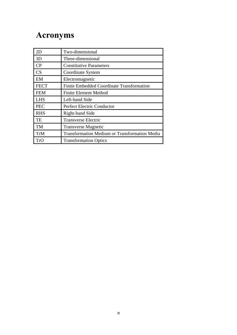
2D Two-dimensional 3D Three-dimensional CP Constitutive Parameters CS Coordinate System EM Electromagnetic FECT Finite Embedded Coordinate Transformation FEM Finite Element Method LHS Left-hand Side PEC Perfect Electric Conductor RHS Right-hand Side TE Transverse Electric TM Transverse Magnetic TrM Transformation Medium or Transformation Media TrO Transformation Optics

XII 

 

1 

1. Introduction 

1.1 Background The method of Transformation Optics (TrO) began to attract wide attention after the publication of

two groundbreaking papers in the same issue of Science magazine [1,2]. Two eye-catching devices

of invisibility cloaks were proposed in these two papers. Invisibility cloaks can make illuminating

light flow around a closed concealment volume, where objects are hidden, and retain the

propagation features of light as if nothing exists in space, so that observers outside the device will

not sense any light/electromagnetic disturbance. To achieve this unusual illusion, both J. B. Pendry

et al. and U. Leonhardt made use of the form invariance of the governing equations, i.e.,

Maxwell’s equations of electromagnetic (EM) theory and Helmholtz equation of geometrical

optics, respectively. Thereafter the equivalence between constitutive parameters (CP) and

geometry for light was established. The techniques were later recognized as transformation optics

in general. The form invariance of Maxwell’s equations and invisible bodies are not new in EM

research (see below for references). However, it is the marriage of the ingredients of TrO and

invisibility that contributes to the significance of the two papers.

As an essential property of Maxwell’s equations (we will focus on the EM theory version of

TrO onwards), the form invariance under transformation of Coordinate Systems (CSs) has already

been studied in several related papers in the 1920s [3-5]. In the early 1960s, Dolin [6], Post [7]

and Lax–Nelso [8] discovered the fundamental idea of TrO. These results, however, have been

forgotten for decades until they were rediscovered in the mid 1990s [9-11]. More detailed

historical review can be found in [12]. Inspired by these previous works, the form invariance is

innovatively applied in the design of invisibility cloaks and plenty of follow-up designs. In most

cases, the desired geometry for light (characteristic of the propagation of light) is specified by

specially conceived coordinate transformations from a virtual space with known light propagation

behavior to the real physical space. The geometry is then embodied by transformation media

(TrM), whose CP are obtained according to the equivalence between CP and transformation. There

are also instances [13-16] where the geometry is described by metrics, borrowing the knowledge

from general relativity. Formally, this metric formulation includes transformation formulation only

as a special case.

Invisibility is commonly known as a popular and fancy factor in science fictions rather than a

serious science or engineering subject. However, there have been in fact various research works

on invisibility for some particular situations, like zero scattering of small ellipsoids [17] and

conductivity invisibility with respect to voltage and current measurements [18,19]. The latter one

utilized the idea of change of variables, sharing the same idea with TrO. Compared with previous

results, the invisibility cloak based on TrO is in the framework of the exact EM theory. Hence, it

can, in principle, be called the perfect invisibility cloak for all spectra of EM waves, including

1. Introduction 

2 

microwave and visible frequencies. The hope for building a true invisibility cloak has been ignited

since the perfect cloak was proposed.

According to the formulation of TrO, the CP of the TrM generally turn out to have high

anisotropy and assume a much broader range of values than exhibited by natural materials. The

experimental realization of TrO generated devices therefore relies heavily on artificial materials,

i.e., metamaterials [20]. The first demonstration of an invisibility cloak [21] was in fact

constructed with split ring resonators, which are the most used unit cells of metamaterials. On the

other hand, until the appearance of TrO, a systematic method for designing metamaterial based

devices was lacking. Now people can exploit the greatest potential of metamaterials by using TrO

to create novel devices which had been otherwise impossible to realize in practice. The mutual

dependence makes TrO and metamaterials closely related to each other.

Months after the first theoretical paper [1], a demonstration of an invisibility cloak based on

metamaterials was reported by D. R. Smith et al. [21]. This experiment triggered the explosion of

research on TrO and invisibility cloaks. The amazing properties of the perfect cloaks attracted

great attention from researchers around the world. A lot of analytical and numerical analysis was

conducted to reveal their interesting characteristics, such as perfection of invisibility [22], EM

scattering in case of imperfection [23], dispersion behavior [24], etc. For a perfect cloak, the

material parameters have very extreme values. The implementation is not possible for natural

materials and is quite difficult even when metamaterials are used. Many simplified or reduced

models [25,26] were then introduced to remove the extreme values. In addition, the working

bandwidth is a serious concern for cloaking operations [27-29]. In the first experimental

demonstration, one of the aforementioned reduced cloaks was fabricated with metamaterials for a

particular EM polarization. Considerable efforts in experimental realization were made towards

higher frequencies, easier fabrication, and better performance [30-34]. Apart from the cloaks with

a closed concealment volume, the curiosity in invisibility leaded people to find other schemes for

cloaking. The following ones were also designed with TrO. Carpet cloaks [35] were much

investigated due to easy fabrication and potential wideband behavior. Geometrical optical cloaking

[2,36,37] based on optical conformal mapping method enables invisibility in the sense of light

rays, but not in the sense of phase unless some negative index media are involved [38]. External

cloaking [39] was achieved by optical cancelling with complementary media. Techniques other

than TrO are used as well. Plasmonic coating induces transparency of particles whose sizes are

small compared with excitation wavelength [40]. Its easy realization with metals in optical spectra

facilitates possible applications of plasmonic cloaking in nanophotonics [41,42]. Microwave

transmission line network cloaks have simple structures, low scattering, and broad operating bands.

However, objects must be small enough to fit into the network grids [43]. Besides passive ones,

active cloaking strategy was proposed in [44]. The incident EM wave (must be known in advance)

is reconstructed by deploying active sources accordingly.

Along with the rapid development of invisibility cloaks, people have developed a growing

1. Introduction 

3 

interest in the theory of TrO. Various applications have been proposed, such as perfect imaging

[45-47], waveguide transition [48,49], beam control [50,51], source manipulation (including

antennas) [52-54], optical illusion [55], singularity transmutation [56] etc. The integration of TrO

with other branches of photonics brings about fruitful results. Transformational plasmonics [57,58]

can help create surface plasmonic devices which are almost free from inelastic scattering. In the

theoretical aspect, TrO has been generalized to include a time variable as well as non-reciprocal

and indefinite media [59-61]. The mathematical formulation implies that such transformation

theory as TrO is valid not only to EM waves, but is more general. The form invariance is actually

ubiquitous for all wave phenomena. Parallel transformation theories have been established for

acoustic [62], elastic [63] and matter waves [64].

1.2 Thesis Outline

The present thesis consists of two parts. In the first part, the background and fundamentals of TrO

and invisibility cloaks are elaborated. In the second part, the author’s research works on TrO and invisibility cloaks are described in detail. Time convention )exp( tiω− is used when working in

frequency domain.

In the first part, the theory of TrO is developed after the background introduction. The

essential idea of TrO is revealed, and working formulas are derived from Maxwell’s equations and

coordinate transformation. The perfect cloak design is treated at last to show how to apply the

theory, and also as a starting point for the invisibility cloak study.

In the second part, the works from our four research papers are discussed. Detailed

description is provided for both the results and the technical methods:

1. A method of designing two-dimensional (2D) reduced cloaks of complex shapes is

proposed. The effectiveness is validated by numerical simulation of an elliptic and a

bowtie-shaped cloak.

2. The concept of inverse transformation optics is introduced to analyze reflection at an

interface of a TrM, which is due to a discontinuous transformation. Necessary and sufficient

condition is obtained for the special situation of no reflection.

3. A half-space cloak is proposed to achieve cloaking above a dielectric ground. Two

carefully designed strips are embedded in the ground for reflection coefficient matching.

4. Carpet cloaking is extended to operation on a dielectric ground. A conformal mapping

generated by a complex function is utilized to calculate the CP.

Finally, the conclusions of the thesis and future work in this field, followed by a summary of

the author’s contributions to the published papers, are given at the end of the thesis.

1. Introduction 

4 

References [1] J. B. Pendry, D. Schurig, and D. R. Smith, “Controlling electromagnetic fields,” Science 312,

1780 (2006).

[2] U. Leonhardt, “Optical conformal mapping,” Science 312, 1777 (2006).

[3] I. E. Tamm, “Electrodynamics of an anisotropic medium in the special theory of relativity,” J.

Russ. Phys. Chem. Soc. 56, 248 (1924).

[4] I. E. Tamm, “Crystal-optics of the theory of relativity pertinent to the geometry of a

biquadratic form,” J. Russ. Phys. Chem. Soc. 57, 1 (1925).

[5] L. I. Mandelstamm and I. E. Tamm, “Elektrodynamik des anisotropen medien und der

speziallen relativitatstheorie,” Math. Ann. 95, 154 (1925).

[6] L. S. Dolin, “On a possibility of comparing three-dimensional electromagnetic systems with

inhomogeneous filling,” Izv. Vyssh. Uchebn. Zaved. Radiofiz. 4, 964 (1961).

[7] E. J. Post, “Formal structure of electromagnetics,” North-Holland (1962).

[8] M. Lax and D. F. Nelson, “Maxwell equations in material form,” Phys. Rev. B 13, 1777

(1976).

[9] W. C. Chew and W. H. Weedon, “A 3d perfectly matched medium from modified Maxwell's

equations with stretched coordinates,” Microw. Opt. Technol. Lett. 7, 599 (1994).

[10] A. J. Ward and J. B. Pendry, “Refraction and geometry in Maxwell’s equations,” J. Mod. Opt.

43, 773 (1996).

[11] A. J. Ward and J. B. Pendry, “Calculating photonic Green’s functions using a nonorthogonal

finite-difference time-domain method,” Phys. Rev. B 58, 7252 (1998).

[12] A. V. Kildishev, W. Cai, U. K. Chettiar, and V. M. Shalaev, “Transformation optics:

approaching broadband electromagnetic cloaking”, New J. of Phys. 10, 115029 (2008).

[13] D. A. Genov, S. Zhang, and X. Zhang, “Mimicking celestial mechanics in metamaterials,” Nat.

Phys. 5, 687 (2009).

[14] M. Li, R. Miao, and Y. Pang, “Casimir energy, holographic dark energy and electromagnetic

metamaterial mimicking de Sitter,” Phys. Lett. B 689, 55 (2010).

[15] T. G. Mackay and A. Lakhtakia, “Towards a metamaterial simulation of a spinning cosmic

string,” Phys. Lett. A 374, 2305 (2010).

[16] I. I. Smolyaninov, and E. E. Narimanov, “Metric Signature Transitions in Optical

Metamaterials,” Phys. Rev. Lett. 105, 067402 (2010).

[17] M. Kerker, “Invisible bodies,” J. Opt. Soc. Am. 65, 376 (1975).

[18] A. Greenleaf, M. Lassas, and G. Uhlmann, “Anisotropic conductivities that cannot be

detected by EIT,” Physiol. Meas. 24, 413 (2003).

[19] A. Greenleaf, M. Lassas, and G. Uhlmann, “On nonuniqueness for Calderons inverse

problem,” Math. Res. Lett. 10, 685 (2003).

[20] Y. Liu, X. Zhang, “Metamaterials: a new frontier of science and technology,” Chem. Soc. Rev.

Advance Article, (2011).

1. Introduction 

5 

[21] D. Schurig, J. J. Mock, B. J. Justice, S. A. Cummer, J. B. Pendry, A. F. Starr, and D. R. Smith,

“Metamaterial electromagnetic cloak at microwave frequencies,” Science 314, 977 (2006).

[22] H. Chen, B. Wu, B. Zhang, and J. Kong, “Electromagnetic wave interactions with a

metamaterial cloak,” Phys. Rev. Lett. 99, 063903 (2007).

[23] Z. Ruan, M. Yan, C. W. Neff, and M. Qiu, “Ideal cylindrical cloak: Perfect but sensitive to tiny

perturbations,” Phys. Rev. Lett. 99, 113903 (2007).

[24] Z. Liang, P. Yao, X. Sun, and X. Jiang, “The physical picture and the essential elements of the

dynamical process for dispersive cloaking structures,” Appl. Phys. Lett. 92, 131118 (2008).

[25] W. Yan, M. Yan, and M. Qiu, “Non-Magnetic Simplified Cylindrical Cloak with Suppressed

Zeroth Order Scattering,” Appl. Phys. Lett. 93, 021909 (2008).

[26] M. Yan, Z. Ruan, and M. Qiu, “Scattering characteristics of simplified cylindrical invisibility

cloaks,” Opt. Express 15, 17772 (2007).

[27] A. V. Kildishev, W. Cai, U. K. Chettiar, and V. M. Shalaev, “Transformation optics:

approaching broadband electromagnetic cloaking,” New J. Phys. 10, 115029 (2008).

[28] H. Chen, Z. Liang, P. Yao, X. Jiang, H. Ma, and C. Chan, “Extending the bandwidth of

electromagnetic cloaks,” Phys. Rev. B 76, 241104 (2007).

[29] H. Hashemi, B. Zhang, J. D. Joannopoulos, and S. G. Johnson, “Delay-Bandwidth and

Delay-Loss Limitations for Cloaking of Large Objects,” Phys. Rev. Lett. 104, 253903 (2010).

[30] R. Liu, C. Ji, J. J. Mock, J. Y. Chin, T. Cui, and D. R. Smith, “Broadband ground-plane cloak,”

Science 323, 366 (2009).

[31] J. Valentine, J. Li, T. Zentgraf, G. Bartal, and X. Zhang, “An optical cloak made of

dielectrics,” Nature Mater. 8, 568 (2009).

[32] H. Ma and T. Cui, “Three-dimensional broadband ground-plane cloak made of

metamaterials,” Nature Commun. 1, doi:10.1038/ncomms1023 (2010).

[33] B. Wood and J. B. Pendry, “Metamaterials at zero frequency,” J. Phys. Condens. Matter 19,

076208 (2007).

[34] C. Li, X. Liu, and F. Li, “Experimental observation of invisibility to a broadband

electromagnetic pulse by a cloak using transformation media based on inductor-capacitor

networks,” Phys. Rev. B 81, 115133 (2010).

[35] J. Li and J. B. Pendry, “Hiding under the carpet: a new strategy for cloaking,” Phys. Rev. Lett.

101, 203901 (2008).

[36] U. Leonhardt and T. Tyc, “Broadband invisibility by non-Euclidean cloaking,” Science 323,

110 (2009).

[37] U. Leonhardt, “Notes on conformal invisibility devices,” New J. Phys. 8, 118 (2006).

[38] T. Ochiai, U. Leonhardt, and J. C. Nacher, “A novel design of dielectric perfect invisibility

devices,” J. Math. Phys. 49, 032903 (2008).

[39] Y. Lai, H. Chen, Z. Zhang, and C. Chan, “Complementary media invisibility cloak that cloaks

objects at a distance outside the cloaking shell,” Phys. Rev. Lett. 102, 093901 (2009).

[40] A. Alù, and N. Engheta, “Achieving Transparency with Plasmonic and Metamaterial

1. Introduction 

6 

Coatings,” Phys. Rev. E 72, 016623 (2005).

[41] A. Alù, and N. Engheta, “Cloaked Near-Field Scanning Optical Microscope Tip for

Noninvasive Near-Field Imaging,” Phys. Rev. Lett. 105, 263906 (2010).

[42] F. Bilotti, S. Tricarico, F. Pierini, and L. Vegni, “Cloaking apertureless near-field scanning

optical microscopy tips,” Opt. Lett. 36, 211 (2011).

[43] S. Tretyakov, P. Alitalo, O. Luukkonen, and C. Simovski, “Broadband electromagnetic

cloaking of long cylindrical objects,” Phys. Rev. Lett. 103, 103905 (2009).

[44] F. G. Vasquez, G. Milton, and D. Onofrei, “Active exterior cloaking for the 2D Laplace and

Helmholtz equations,” Phys. Rev. Lett. 103, 073901 (2009).

[45] N. Kundtz and D. R. Smith, “Extreme-angle broadband metamaterial lens,” Nat. Mater. 9, 129

(2010).

[46] D. Schurig, “An aberration-free lens with zero F-number,” New J. Phys. 10, 115034 (2008).

[47] A. V. Kildishev and E. E. Narimanov, “Impedance-matched hyperlens,” Opt. Lett. 32, 3432

(2007).

[48] O. Ozgun and M. Kuzuoglu, “Utilization of anisotropic metamaterial layers in waveguide

miniaturization and transitions,” IEEE Microw. Wirel. Compon. Lett. 17, 754 (2007).

[49] B. Donderici and F. L. Teixeira, “Metamaterial blueprints for reflectionless waveguide

bends,” IEEE Microw. Wirel. Compon. Lett. 18, 233 (2008).

[50] X. Xu, Y. Feng, and T. Jiang, “Electromagnetic beam modulation through transformation

optical structures,” New J. Phys. 10, 115027 (2008).

[51] M. Rahm, D. A. Roberts, J. B. Pendry, and D. R. Smith, “Transformation-optical design of

adaptive beam bends and beam expanders,” Opt. Express 16, 11555 (2008).

[52] N. Kundtz, D. A. Roberts, J. Allen, S. Cummer, and D. R. Smith, “Optical source

transformations,” Opt. Express 16, 21215 (2008).

[53] S. A. Cummer, N. Kundtz, and B. I. Popa, “Electromagnetic surface and line sources under

coordinate transformations,” Phys. Rev. A 80, 033820 (2009).

[54] P. H. Tichit, S. N. Burokur, and A. de Lustrac, “Ultradirective antenna via transformation

optics,” J. Appl. Phys. 105, 104912 (2009).

[55] Y. Lai, J. Ng, H. Chen, D. Han, J. Xiao, Z. Zhang, and C. Chan, “Illusion optics: the optical

transformation of an object into another object,” Phys. Rev. Lett. 102, 253902 (2009).

[56] T. Tyc and U. Leonhardt, “Transmutation of singularities in optical instruments,” New J. Phys.

10, 1 (2009).

[57] P. A. Huidobro, M. L. Nesterov, L. Martín-Moreno, and F. J. García-Vidal, “Transformation

optics for plasmonics,” Nano Lett. 10, 1985 (2010).

[58] Y. Liu, T. Zentgraf, G. Bartal, and X. Zhang, “Transformational plasmon optics,” Nano Lett.

10, 1991 (2010).

[59] L. Bergamin, “Generalized transformation optics fromtriple spacetime metamaterials,” Phys.

Rev. A 78, 043825 (2008).

[60] R. T. Thompson, S. A. Cummer, and J. Frauendiener, “A completely covariant approach to

1. Introduction 

7 

transformation optics,” J. Opt. 13, 024008 (2011).

[61] S. A. R. Horsley, “Transformation optics, isotropic chiral media, and non-Riemannian

geometry,” arXiv:1101.1755v2, (2011).

[62] S. A. Cummer, B. I. Popa, D. Schurig, D. R. Smith, J. Pendry, M. Rahm, and A. Starr,

“Scattering Theory Derivation of a 3D Acoustic Cloaking Shell,” Phys. Rev. Lett. 100,

024301 (2008).

[63] M. Farhat, S. Guenneau and S. Enoch, “Ultrabroadband Elastic Cloaking in Thin Plates,”

Phys. Rev. Lett. 103, 024301 (2009).

[64] S. Zhang, D. A. Genov, C. Sun, and X. Zhang, “Cloaking of matter waves,” Phys. Rev. Lett.

100, 123002 (2008).

1. Introduction 

8 

 

9 

2. Theory of Transformation Optics

The fundamental theory of TrO is developed by starting from Maxwell’s equations and a coordinate

transformation between two spaces. Multivariable calculus is enough for the derivation of all

formulas. Necessary concepts from differential geometry will be clearly defined and explained.

The theoretical model of EM media discussed in the present thesis is limited to be linear and

anisotropic. Time dependent and magnetoelectric responses of materials are not considered here,

but can be included in generalized formulations (see Section 1.1 Background). The derivation of

TrO has been treated in literature [1-3]. However, it is still helpful to formulate the theory with

consistent notations, so that the thesis is self-contained as a complete work. The last section will

describe the design procedure of TrO and show how the geometrical features of transformations

are embodied for light by TrM. Perfect cloaks are taken as an example.

2.1 Elements of Coordinate Transformation In the mathematical language, the theory of TrO discusses the relation between quantities in two

spaces, whose coordinate variables are connected by a coordinate transformation. The CSs used in

the two spaces do not depend on what the transformation is, and therefore can be chosen for

convenience. Here, Cartesian CS is adopted for both spaces in the current development for its

simplicity. Results for other orthogonal CSs are obtained in Section 2.3 by linking to the current

Cartesian coordinate case. Quantities in the spaces can be given physical meanings when they

satisfy corresponding governing equations. Although the two spaces are mathematically identical,

we would like to distinguish them by names of virtual space and physical space according to their

roles in TrO. Quantities in the physical space are denoted by notations with prime, while no

primes are associated with the virtual space.

Assume the coordinate variables of the two spaces are related by the transformation function  

( )' ' ,=r r r (2.1)

where ' ' 'iip=r x   and i

ip=r x   are radius vectors expanded with vector bases of Cartesian CSs.

The transformation expressed in component form looks like

( )1 2 3' ' , , .i ip p p p p=

Before moving on we would like to state some conventions of index usage at an early stage

to avoid any possible confusion caused by index notations. Single (stand alone) indices are usually

meant to represent a whole set of quantities by taking all possible index values (1, 2 and 3). A

same index occurring twice, one subscript and one superscript, implies a summation with the

index running over all possible values (Einstein summation convention). Whether subscript or

superscript should be used follows the rules of tensor notation, which are explained later in this

2. Theory of Transformation Optics 

10 

section. These conventions ensure that indices in a physical formula are always balanced, i.e., both

sides of the equation have the same indices at the same positions.

The two CSs have the same role in the coordinate transformation. Equivalent to Eq.(2.1), the

coordinate variables in the virtual space are also functions of those in the physical space. For most

applications, transformations are differential and the Jacobian matrices (see below, Eq. (2.9)) are

not singular, i.e., the function systems are invertible. We note that the set of coordinate variables in

one space, say the physical space, can be interpreted as another CS (usually curvilinear) in the

other space, the virtual space. The coordinate grid lines of (p'1, p'2) can be drawn in the virtual

space to represent the transformation geometrically as illustrated in Fig. 2.1(a) (the coordinate grid

lines of (p'1, p'2) in the physical space are also shown in Fig. 2.1(b) for comparison). Quantities in

the virtual space are thus also functions of the curvilinear coordinate variables.

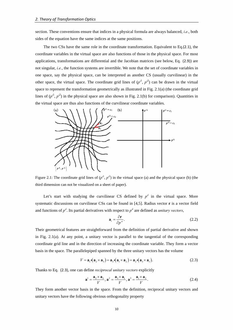
Figure 2.1: The coordinate grid lines of (p'1, p'2) in the virtual space (a) and the physical space (b) (the

third dimension can not be visualized on a sheet of paper).

Let’s start with studying the curvilinear CS defined by p'i in the virtual space. More

systematic discussions on curvilinear CSs can be found in [4,5]. Radius vector r is a vector field

and functions of p'i. Its partial derivatives with respect to p'i are defined as unitary vectors,

.'i ip

∂=∂

ra (2.2)

Their geometrical features are straightforward from the definition of partial derivative and shown

in Fig. 2.1(a). At any point, a unitary vector is parallel to the tangential of the corresponding

coordinate grid line and in the direction of increasing the coordinate variable. They form a vector

basis in the space. The parallelepiped spanned by the three unitary vectors has the volume

( ) ( ) ( )1 2 3 3 1 2 2 3 1 .V = × = × = ×a a a a a a a a ai i i (2.3)

Thanks to Eq. (2.3), one can define reciprocal unitary vectors explicitly

1 2 32 3 3 1 1 2, , .V V V× × ×

= = =a a a a a a

a a a (2.4)

They form another vector basis in the space. From the definition, reciprocal unitary vectors and

unitary vectors have the following obvious orthogonality property

2. Theory of Transformation Optics 

11 

,i ij jδ=a ai (2.5)

where subscript and superscript indicate unitary and reciprocal unitary vectors respectively, and

ijδ is the Kronecker delta symbol. The total differential change in radius vector can be expressed

as the sum of all partial differential changes,

' .iid dp=r a (2.6)

Eq. (2.6) is for the most general case (with differential changes in all coordinate variables). If there

is only differential change in one coordinate variable, one term in the equation suffices to

represent the differential change in r. Reciprocal unitary vector basis can also be used for

expansion

' ,iid dp=r a (2.7)

which acts as the definition of the components dp'i.

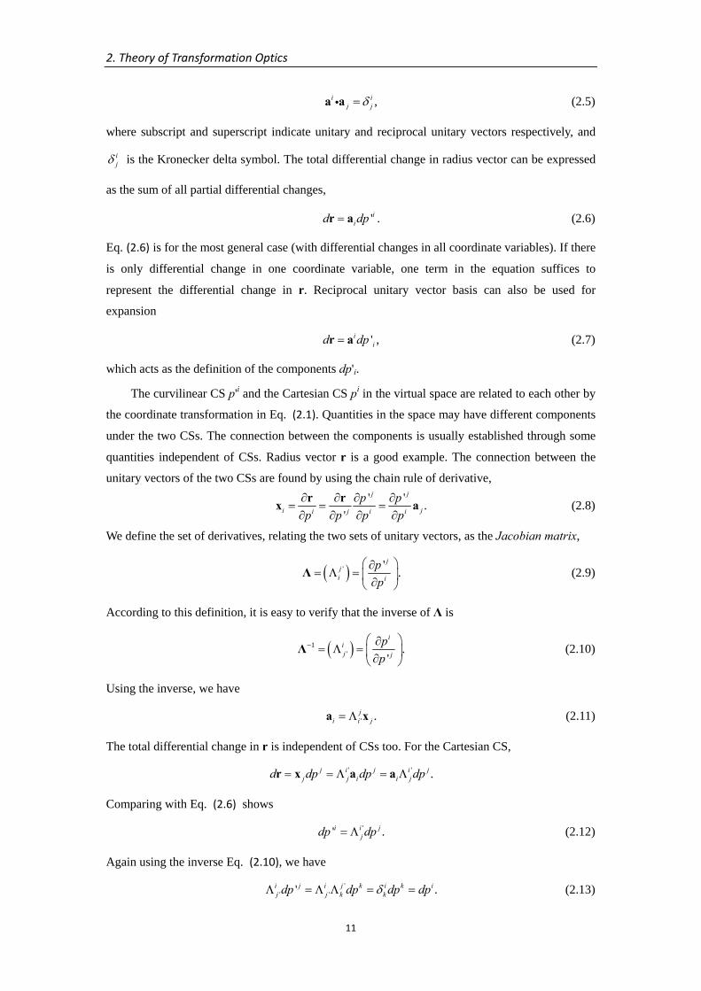
The curvilinear CS p'i and the Cartesian CS pi in the virtual space are related to each other by

the coordinate transformation in Eq. (2.1). Quantities in the space may have different components

under the two CSs. The connection between the components is usually established through some

quantities independent of CSs. Radius vector r is a good example. The connection between the

unitary vectors of the two CSs are found by using the chain rule of derivative,

' ' .'

j j

i ji j i i

p pp p p p∂ ∂ ∂ ∂

= = =∂ ∂ ∂ ∂

r rx a (2.8)

We define the set of derivatives, relating the two sets of unitary vectors, as the Jacobian matrix,

( )' ' .j

ji i

pp

⎛ ⎞∂= Λ = ⎜ ⎟∂⎝ ⎠

Λ (2.9)

According to this definition, it is easy to verify that the inverse of Λ is

( )1' .

'

iij j

pp

− ⎛ ⎞∂= Λ = ⎜ ⎟∂⎝ ⎠

Λ (2.10)

Using the inverse, we have

' .ji i j= Λa x (2.11)

The total differential change in r is independent of CSs too. For the Cartesian CS,

' ' .j i j i jj j i i jd dp dp dp= = Λ = Λr x a a

Comparing with Eq. (2.6) shows

'' .i i jjdp dp= Λ (2.12)

Again using the inverse Eq. (2.10), we have

'' '' .i j i j k i k i

j j k kdp dp dp dpδΛ = Λ Λ = = (2.13)

2. Theory of Transformation Optics 

12 

Eqs. (2.11) and (2.12) present two different ways of transformation from the Cartesian CS to the

curvilinear CS. Quantities that transform like ai are covariant, and quantities that transform like

dp'i are contravariant. The positions of indices are designed to manifest the distinct ways of

transformation. Subscript and superscript indices indicate covariant and contravariant, respectively.

More than one index may be needed to denote components of a complex quantity. In general, a

quantity, whose components follow the two transformation rules with respect to all the indices, is

called a tensor. A quantity without index and invariant of CSs is a scalar, the zero-th order tensor.

To see if a quantity is a tensor, we should identify how the components transform by using its

physical or geometrical properties and check against the two rules. Indices for all the tensors we

have encountered are placed properly according to their tensorial nature.

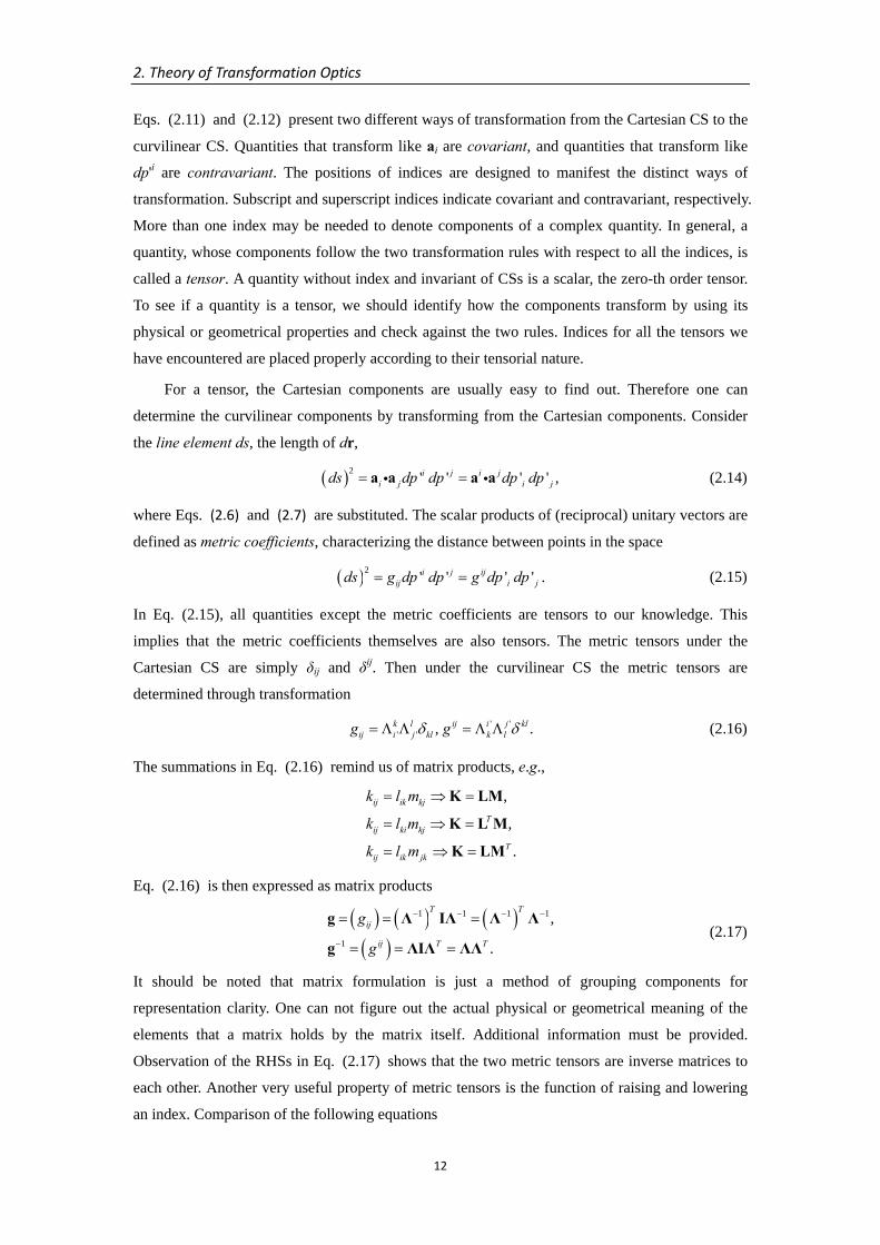
For a tensor, the Cartesian components are usually easy to find out. Therefore one can

determine the curvilinear components by transforming from the Cartesian components. Consider

the line element ds, the length of dr,

( )2 ' ' ' ' ,i j i ji j i jds dp dp dp dp= =a a a ai i (2.14)

where Eqs. (2.6) and (2.7) are substituted. The scalar products of (reciprocal) unitary vectors are

defined as metric coefficients, characterizing the distance between points in the space

( )2 ' ' ' ' .i j ijij i jds g dp dp g dp dp= = (2.15)

In Eq. (2.15), all quantities except the metric coefficients are tensors to our knowledge. This

implies that the metric coefficients themselves are also tensors. The metric tensors under the

Cartesian CS are simply δij and δij. Then under the curvilinear CS the metric tensors are

determined through transformation

' '' ' , .k l ij i j kl

ij i j kl k lg gδ δ= Λ Λ = Λ Λ (2.16)

The summations in Eq. (2.16) remind us of matrix products, e.g.,

,

,

.

ij ik kj

Tij ki kj

Tij ik jk

k l m

k l m

k l m

= ⇒ =

= ⇒ =

= ⇒ =

K LM

K L M

K LM

Eq. (2.16) is then expressed as matrix products

( ) ( ) ( )( )

1 1 1 1

1

,

.

T T

ij

ij T T

g

g

− − − −

−

= = =

= = =

g Λ IΛ Λ Λ

g ΛIΛ ΛΛ (2.17)

It should be noted that matrix formulation is just a method of grouping components for

representation clarity. One can not figure out the actual physical or geometrical meaning of the

elements that a matrix holds by the matrix itself. Additional information must be provided.

Observation of the RHSs in Eq. (2.17) shows that the two metric tensors are inverse matrices to

each other. Another very useful property of metric tensors is the function of raising and lowering

an index. Comparison of the following equations

2. Theory of Transformation Optics 

13 

' ' ,

' ' ' ,

' ' ' ,

' ' ,

j ji i j ij

j ji i j i j i

i i j i j ij j

i i j ijj j

d dp g dp

d dp dp dp

d dp dp dp

d dp g dp

δ

δ

= =

= = =

= = =

= =

a r a a

a r a a

a r a a

a r a a

i i

i i

i i

i i

proves to us

' ' , ' ' .j ij iij i jg dp dp g dp dp= = (2.18)

Unitary vectors, having metric tensors as their scalar products, generally do not have unit lengths.

Their corresponding unit vectors are obtained by normalization

, .i i

ii ii i i ii

i i iig g= = = =

a a a au ua a a ai i

Considering the unity magnitudes of these vectors, it is sometimes convenient to use them as bases

for vector expansion. However, the unit vectors and the corresponding expansion components do

not transform like tensors.

The volume in Eq. (2.3) is important when determining the differential volume element, and

will be frequently used in the next section. By applying the similar technique for calculating the

metric tensors, we get a useful formula for the volume. Substitute Eq. (2.11) into Eq. (2.3),

( ) ( )1' 2 ' 3' 1' 2 ' 3' .i j k i j ki j k i j kV = Λ Λ ×Λ = Λ Λ Λ ×x x x x x xi i (2.19)

The triple scalar products of the Cartesian unitary vectors take nonvanishing values ±1 when [i, j,

k] is a permutation of the set {1, 2, 3}, and the sign depends on the signature of the permutation.

The RHS of Eq. (2.19) is just the determinant of Λ–1 by definition, i.e.,

( ) ( )1det sgn .V V g−= =Λ (2.20)

The last step results from the fact ( ) ( ) 21det detg −⎡ ⎤= = ⎣ ⎦g Λ implied by Eq. (2.17). The sign can

be easily decided according to Eq. (2.3), positive for a right-hand CS and negative for a left-hand

CS.

2.2 The Form Invariance of Maxwell’s Equations

Equipped with the toolbox of coordinate transformation developed in Section 2.1, we are now ready

to treat the core part of TrO, namely, the form invariance of Maxwell’s equations. We are moving on

to work with the two spaces, the virtual space and the physical space, introduced in Section 2.1. The

two spaces are equivalently related by the coordinate transformation Eq. (2.1), but play different

roles when EM fields are introduced. The virtual space is assumed to be filled with an anisotropic

medium with the CP (ε, μ) and have known EM fields characterized by (E, H, D, B) in it. The EM

fields satisfy Maxwell’s equations and the constitutive relations,

2. Theory of Transformation Optics 

14 

,t

∂∇× = −

∂BE (2.21)

,t

∂∇× = +

∂DH J (2.22)

,ρ∇ =Di (2.23)

0,∇ =Bi (2.24)

, .= =D εE B μH (2.25)

These physical quantities, including fields, sources and CP, are independent of CSs, but may have

different components when expressed in terms of different vector bases, e.g.,

.i i ii i id d D= = =D a a x (2.26)

By the form invariance under a coordinate transformation, we attempt to construct a new set of

EM fields, sources and CP in the physical space from those in the virtual space, so that in the

physical space the form of Maxwell’s equations is conserved for the new set. The medium

specified by the new set in the physical space is called a transformation medium. In practice, it is

the TrM that is fabricated to realize desired EM properties. That’s why this space is called physical

space, while the other space is called virtual space.

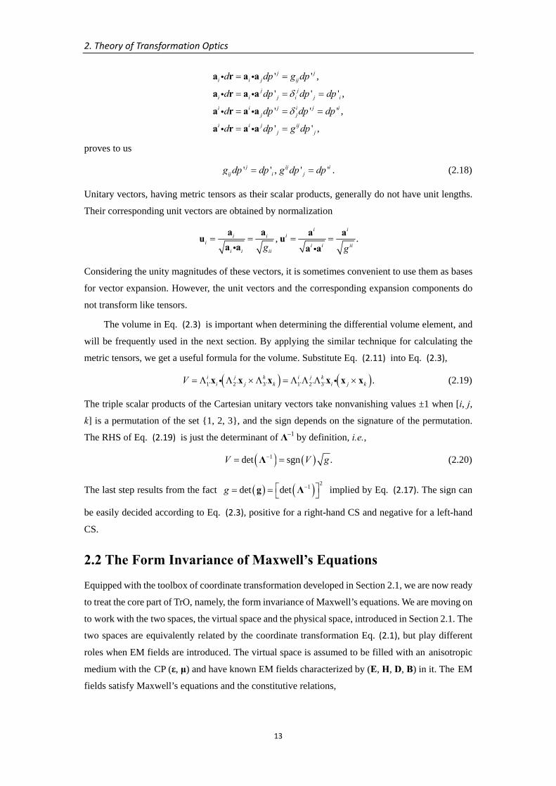
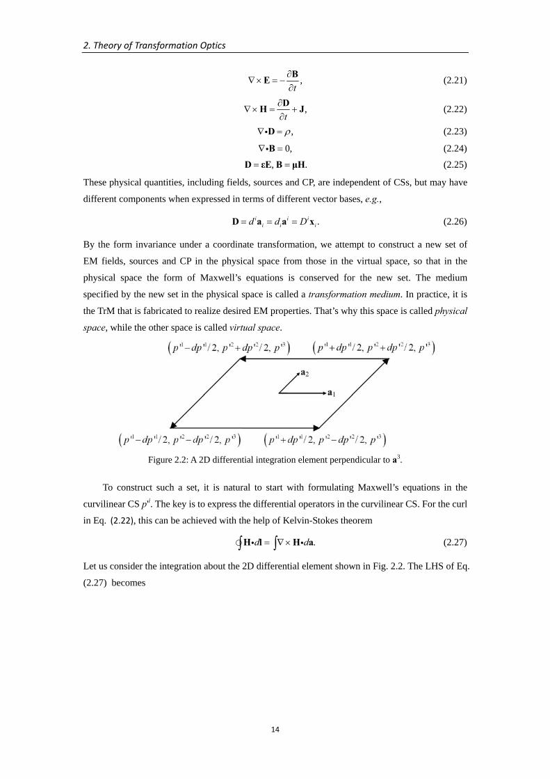
Figure 2.2: A 2D differential integration element perpendicular to a3.

To construct such a set, it is natural to start with formulating Maxwell’s equations in the

curvilinear CS p'i. The key is to express the differential operators in the curvilinear CS. For the curl

in Eq. (2.22), this can be achieved with the help of Kelvin-Stokes theorem

.d d= ∇×∫ ∫H l H ai i (2.27)

Let us consider the integration about the 2D differential element shown in Fig. 2.2. The LHS of Eq.

(2.27) becomes

2. Theory of Transformation Optics 

15 

( ) ( )( ) ( )

( ) ( )

( )

2 2 1 1

2 2 1 1

1 21 2' ' /2 ' ' /2

1 21 2' ' /2 ' ' /2

1 22 11 21 2

1 22 1

1 211 2

1 22

' '

' '

' '' '' '' 2 ' 2

' '' '' 2

p dp p dp

p dp p dp

d dp dp

dp dp

dp dpdp dpdp dpp p

dp dpdp dpp

− +

+ −

= +

− −

⎡ ⎤ ⎡ ⎤∂ ∂⎢ ⎥ ⎢ ⎥= − + +

∂ ∂⎢ ⎥ ⎢ ⎥⎣ ⎦ ⎣ ⎦⎡ ⎤∂⎢ ⎥− + − −

∂⎢ ⎥⎣ ⎦

∫ H r H a H a

H a H a

H a H aH a H a

H aH a H a

i i i

i i

i ii i

ii i

( )2 12

1

1 1 2 2 1 21 21 22 1

1 1 2 2 1 21 21 22 1

1 22 11 2

' '' 2

1 1' ' ' ' ' '2 ' 2 '

1 1' ' ' ' ' '2 ' 2 '

' ' ,' '

dp dpp

h hh dp dp dp h dp dp dpp p

h hh dp dp dp h dp dp dpp p

h h dp dpp p

⎡ ⎤∂⎢ ⎥

∂⎢ ⎥⎣ ⎦⎛ ⎞ ⎛ ⎞∂ ∂

= − + +⎜ ⎟ ⎜ ⎟∂ ∂⎝ ⎠ ⎝ ⎠⎛ ⎞ ⎛ ⎞∂ ∂

− + − −⎜ ⎟ ⎜ ⎟∂ ∂⎝ ⎠ ⎝ ⎠⎛ ⎞∂ ∂

= −⎜ ⎟∂ ∂⎝ ⎠

H ai (2.28)

where hi are the covariant components of the magnetic field. In Eq. (2.28), the scalar product

along every one of the four laterals is obtained by adding a variational part to that evaluated at the

element center p'i. The RHS of Eq. (2.27) is

( ) ( )1 21 2' ' .d dp dp∇× = ∇× ×∫ H a H a ai i

Eq. (2.27) is then simplified to

( ) ( ) 2 11 2 1 2 .

' 'h hp p∂ ∂

∇× × = −∂ ∂

H a ai (2.29)

Note that p'i is a Cartesian CS in the physical space. Thus the RHS of Eq. (2.29) is just the 3rd

Cartesian component of curl operator in the physical space. hi are accordingly recognized as the

Cartesian components of the magnetic field in the physical space,

' .i iH h= (2.30)

The LHS and the RHS being from different spaces, Eq. (2.30) is only a numerical equality without

physical implication. In a Cartesian CS, all vector bases (unit or unitary) coincide into a constant

basis. For the Cartesian components H'i, the index position does not make any difference. Here

subscript is used for the sake of formal index balance. Substitute the definition Eq. (2.30) into Eq.

(2.29),

( ) ( ) ( )32 11 2 1 2

' ' ' ' .' '

H Hp p

∂ ∂∇× × = − = ∇ ×

∂ ∂H a a Hi (2.31)

Parallel studies for Eq. (2.21) will result in the counterpart definition of the electric field in the

physical space

' ,i iE e= (2.32)

where ei are the covariant components of the electric field in the virtual space. As for the LHS of

Eq. (2.29), substitution of Eq. (2.22) leads to

2. Theory of Transformation Optics 

16 

( ) ( ) ( )1 2 1 2 .t

∂⎛ ⎞∇× × = + ×⎜ ⎟∂⎝ ⎠

DH a a J a ai i

Expand D and J with the vector basis ai and only one term survives according to Eqs. (2.3) and

(2.20),

( ) ( ) ( )

( ) ( )

1 2 1 2

3 33 3 1

3 1 2 det .

ii

id jt

d dj jt t

−

⎛ ⎞∂∇× × = + ×⎜ ⎟∂⎝ ⎠⎛ ⎞ ⎛ ⎞∂ ∂

= + × = +⎜ ⎟ ⎜ ⎟∂ ∂⎝ ⎠ ⎝ ⎠

H a a a a a

a a a Λ

i i

i

Eliminate d3 with the constitutive relation D = ε E,

3 3' 3' 3' 3'' ' .i i j i j k i j kl

i i j i j k i j k ld D E e g eε ε ε= Λ = Λ = Λ Λ = Λ Λ

Here we use the Cartesian components of the permittivity tensor. The contravariant component d3 is

first expressed in terms of the Cartesian components Di by using Eqs. (2.11) and (2.26). After

applying the constitutive relation, the Cartesian components Ej are replaced by expressions of

curvilinear components. Put d3 back and replace el with E'l (Eq. (2.32)),

( ) ( ) ( ) ( )3' 1 1 31 2 '

'det det .i j kl l

i j kE

g jt

ε − −∂∇× × = Λ Λ +

∂H a a Λ Λi (2.33)

Combine Eqs. (2.31) and (2.33),

( ) ( ) ( )3 3' 1 1 3'

'' ' det det .i j kl l

i j kE

g jt

ε − −∂∇ × = Λ Λ +

∂H Λ Λ (2.34)

Eq. (2.34) infers

( ) ( ) ( )' 1 1'

'' ' det det .m m i j kl ml

i j kE

g jt

ε − −∂∇ × = Λ Λ +

∂H Λ Λ (2.35)

In order to establish the form invariance, we define the electric current density by its Cartesian

components

( )1' det .m mJ j−= Λ (2.36)

Eq. (2.35) then can be written in matrix form

( )

( )

1 1 1

1

'' ' det '

'det '.T

t

t

− − −

−

∂∇ × = +

∂∂

= +∂

EH ΛεΛ g Λ J

EΛεΛ Λ J (2.37)

Eq. (2.37) assumes the same form as Eq. (2.22) as long as the following permittivity tensor for the

TrM is introduced,

( )1' det .T −=ε ΛεΛ Λ (2.38)

The magnetic permeability tensor can be similarly obtained by studying the other curl equation in

Maxwell’s equations,

( )1' det .T −=μ ΛμΛ Λ (2.39)

Eq. (2.37) finally turns out to be,

2. Theory of Transformation Optics 

17 

'' ' ' '.t

∂∇ × = +

∂EH ε J (2.40)

In Eqs. (2.30), (2.32) and (2.36), curvilinear components are used for definition. In practice, it is more convenient to use Cartesian components, which are independent of the curvilinear CS. Using Eqs. (2.11) and (2.12), the curvilinear components are expressed in terms of Cartesian components,

( ) ( )1 ' 1' '' , ' , ' det det .j j i i i j

i i i j i i i j jE e E H h E J j J− −= = Λ = = Λ = = ΛΛ Λ

They are further put in matrix form,

( ) ( ) ( )1 1 1' , ' , ' det .T T− − −= = =E Λ E H Λ H J Λ Λ J (2.41)

The same results as above can be derived by another similar but shorter method. Starting from

Eq. (2.31), expand ∇×H into

( ) ( ) ,i ii i∇× = ∇× = ∇×H h a H x (2.42)

where the notation ( )i∇×h is coined to denote the curvilinear components of ∇×H , and does

not mean a curl operation. The two sets of the components are related by

( ) ( )' .i jij∇× = Λ ∇×h H (2.43)

Inserting Eqs. (2.42) and (2.43), Eq. (2.31) becomes

( ) ( ) ( )

( )( ) ( ) ( )

31 2

31 1 3'

' '

det det .

ii

jj

− −

∇ × = ∇× ×

= ∇× = Λ ∇×

H h a a a

Λ h Λ H

i

It can be inferred

( ) ( ) ( )1 '' ' det .i jij

−∇ × = Λ ∇×H Λ H

Put it in matrix form,

( )1' ' det .−∇ × = ∇×H Λ Λ H (2.44)

Substitute Eq. (2.22) into Eq. (2.44),

( ) ( )

( )

( ) ( )

1 1

1

1 1

' ' det det

'det

'det det .

T

T

t t

t

t

− −

−

− −

∂ ∂⎛ ⎞ ⎛ ⎞∇ × = + = +⎜ ⎟ ⎜ ⎟∂ ∂⎝ ⎠ ⎝ ⎠∂⎛ ⎞= +⎜ ⎟∂⎝ ⎠

∂= +

∂

D εEH Λ Λ J Λ Λ J

EΛ Λ εΛ J

EΛ ΛεΛ Λ ΛJ

From the above equation, we find that the permittivity tensor of the TrM and the current density in

the physical space are the same as the previous results.

2. Theory of Transformation Optics 

18 

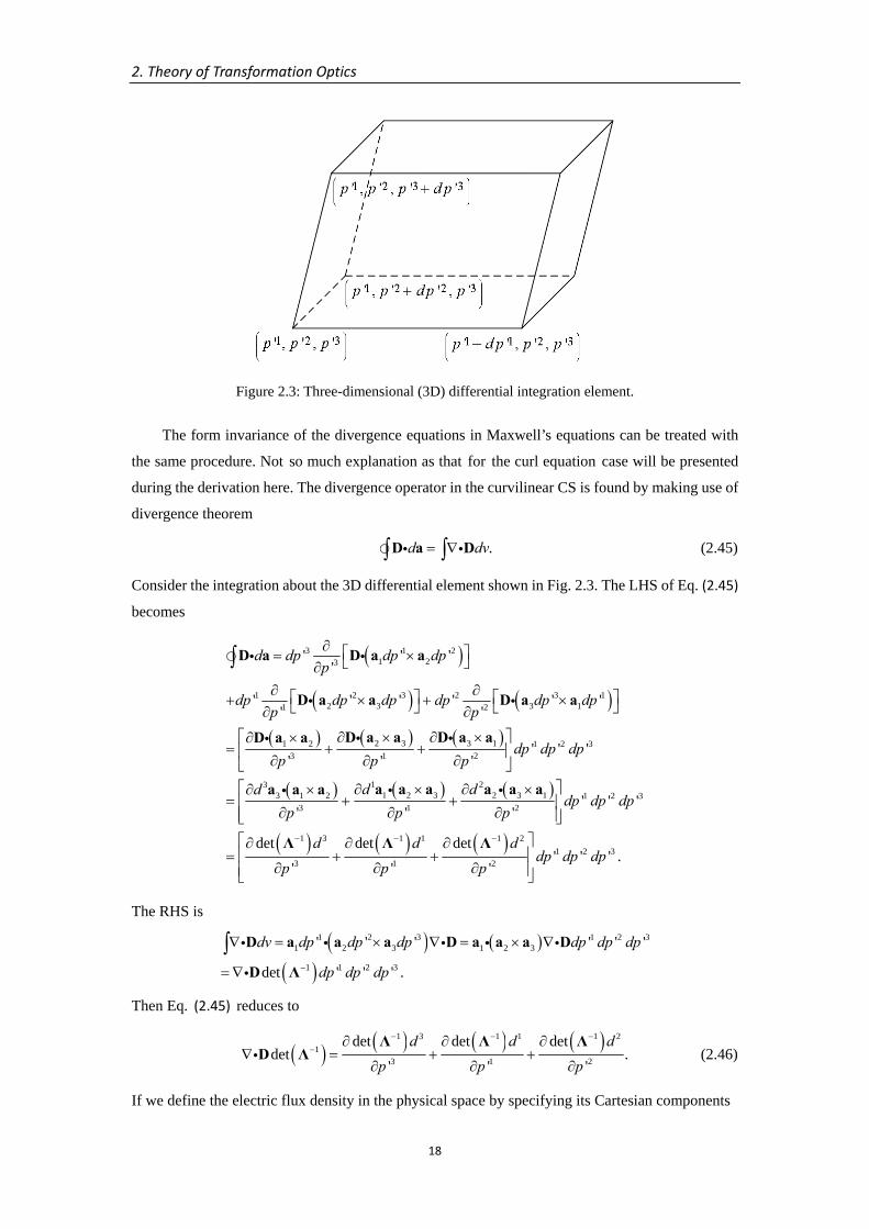
Figure 2.3: Three-dimensional (3D) differential integration element.

The form invariance of the divergence equations in Maxwell’s equations can be treated with

the same procedure. Not so much explanation as that for the curl equation case will be presented

during the derivation here. The divergence operator in the curvilinear CS is found by making use of

divergence theorem

.d dv= ∇∫ ∫D a Di i (2.45)

Consider the integration about the 3D differential element shown in Fig. 2.3. The LHS of Eq. (2.45)

becomes

( )

( ) ( )( ) ( ) ( )

( ) ( ) ( )

3 1 21 23

1 2 3 2 3 12 3 3 11 2

2 3 3 11 2 1 2 33 1 2

1 231 2 3 2 3 13 1 2

3 1 2

' ' ''

' ' ' ' ' '' '

' ' '' ' '

' ' '

d dp dp dpp

dp dp dp dp dp dpp p

dp dp dpp p p

d ddp p p

∂ ⎡ ⎤= ×⎣ ⎦∂∂ ∂⎡ ⎤ ⎡ ⎤+ × + ×⎣ ⎦ ⎣ ⎦∂ ∂

⎡ ⎤∂ × ∂ ×∂ ×= + +⎢ ⎥∂ ∂ ∂⎣ ⎦⎡ ∂ × ∂ ×∂ ×

= + +∂ ∂ ∂⎣

∫ D a D a a

D a a D a a

D a a D a aD a a

a a a a a aa a a

i i

i i

i ii

i ii

( ) ( ) ( )

1 2 3

1 3 1 1 1 21 2 3

3 1 2

' ' '

det det det' ' ' .

' ' '

dp dp dp

d d ddp dp dp

p p p

− − −

⎤⎢ ⎥⎢ ⎥⎦⎡ ⎤∂ ∂ ∂⎢ ⎥= + +

∂ ∂ ∂⎢ ⎥⎣ ⎦

Λ Λ Λ

The RHS is

( ) ( )

( )

1 2 3 1 2 31 2 3 1 2 3

1 1 2 3

' ' ' ' ' '

det ' ' ' .

dv dp dp dp dp dp dp

dp dp dp−

∇ = × ∇ = × ∇

= ∇

∫ D a a a D a a a D

D Λ

i i i i i

i

Then Eq. (2.45) reduces to

( ) ( ) ( ) ( )1 3 1 1 1 21

3 1 2

det det detdet .

' ' '

d d d

p p p

− − −−

∂ ∂ ∂∇ = + +

∂ ∂ ∂

Λ Λ ΛD Λi (2.46)

If we define the electric flux density in the physical space by specifying its Cartesian components

2. Theory of Transformation Optics 

19 

( )1' det ,i iD d−= Λ (2.47)

Eq. (2.46) gives

( )1' ' det .−∇ = ∇D Λ Di i (2.48)

Substitute Eq. (2.23) into Eq. (2.48),

( )1' ' det .ρ−∇ =D Λi (2.49)

Then the electric charge density in the physical space is

( )1' det .ρ ρ−= Λ (2.50)

Express the curvilinear components in the definition Eq. (2.47) in terms of Cartesian components,

( ) ( )1 1 '' det det .i i i jjD d D− −= = ΛΛ Λ

Then Eq. (2.47) can be written in matrix form

( )1' det .−=D Λ ΛD (2.51)

Study of the other divergence equation results in the definition of the magnetic flux density in the

physical space

( )1' det .−=B Λ ΛB (2.52)

So far, we have constructed the set of EM fields, sources and TrM in the physical space by using

the form invariance of Maxwell’s equations. The complete list is given below for quick reference

( ) ( )1 1' , ' ,T T− −= =E Λ E H Λ H (2.41)

( )1' det ,−=D Λ ΛD (2.51)

( )1' det ,−=B Λ ΛB (2.52)

( )1' det ,−=J Λ Λ J (2.41)

( )1' det ,ρ ρ−= Λ (2.50)

( )1' det ,T −=ε ΛεΛ Λ (2.38)

( )1' det .T −=μ ΛμΛ Λ (2.39)

Besides, the current continuity equation can be easily proven form invariant as well. From Eqs.

(2.41), (2.51) and (2.52), we note that the current density and the flux densities follow the same

transformation rule, and thus Eq. (2.48) also applies for current density,

( )1' ' det .−∇ = ∇J Λ Ji i (2.53)

2. Theory of Transformation Optics 

20 

The form invariance then can be clearly seen with Eqs. (2.50) and (2.53). Considering the duality of

the EM theory, it is not surprising to have the same form of the results pertinent to electric and

magnetic fields. From this section on, we will only present discussions for one case for brevity.

2.3 Transformation Optics with Orthogonal Coordinates

In the previous section, the fundamental theory of TrO has been derived. In the formulation, the

relation of the two spaces is characterized by a transformation between Cartesian CSs and the results

are expressed with Cartesian components. However in many situations, other orthogonal CSs (e.g.,

cylindrical and spherical CSs) are very convenient for coordinate transformation and geometrical

shape description. The Cartesian formulation of TrO becomes awkward in these situations. To take

advantage of the convenience offered by orthogonal CSs, this section is devoted to building a

formulation of TrO based on general orthogonal CSs.

First of all, we introduce two general orthogonal CSs, qi and q'i, in the virtual space and the

physical space, respectively. Note that the two CSs are not necessarily of the same form, although

most of the time they are. As a special kind of curvilinear CSs, orthogonal CSs are just like p'i we

have thoroughly investigated in Section 2.1. The properties of the curvilinear CS p'i apply for q'i and

qi as well. Apart from the general properties for curvilinear CSs, unitary vectors of an orthogonal

CS, say qi, are orthogonal to each other. The metric tensor is thus diagonal,

( ) ( ) 221 2 3, , ,ij i j i ijg h diag h h hδ ⎡ ⎤= = ⇒ = ⎣ ⎦b b gi (2.54)

where bi are the unitary vectors of the CS qi. i i ih = b bi   in the above equations are called scale

factors. They are not components of a tensor, and therefore the indices are not counted in with

regard to index balance and summation.

The relation between the two spaces is specified by a transformation between the orthogonal

CSs,

( )1 2 3' ' , , .i iq q q q q= (2.55)

The Jacobian matrix is

( ) ' .i

ij j

qq

λ⎛ ⎞∂

= = ⎜ ⎟∂⎝ ⎠λ

The Jacobian matrix utilized in the Cartesian formulation of TrO is for the transformation between

the Cartesian CSs. It can be calculated as

' ' ' ' ' ' .' '

i i k i k lij j k j k l j

p p q p q qp q p q q p∂ ∂ ∂ ∂ ∂ ∂

Λ = = =∂ ∂ ∂ ∂ ∂ ∂

(2.56)

If we define the Jacobian matrix of the orthogonal CS qi with respect to the Cartesian CS pi

,i

j

qp

⎛ ⎞∂= ⎜ ⎟∂⎝ ⎠

T

2. Theory of Transformation Optics 

21 

Eq. (2.56) can be written in matrix form as

1' .−=Λ T λT (2.57)

In the orthogonal CS qi, the constitutive relation for electric flux density and electric field becomes

i i jjd eε= (2.58)

in component form ( id and je are the contravariant components) or

=d εe (2.59)

in matrix form. The permittivity tensor in orthogonal components can be transformed to that in

Cartesian components according to the tensor transformation rules,

,i l

i kj lk j

p qq p

ε ε∂ ∂=∂ ∂

which is equivalent to

1 .−=ε T εT (2.60)

Now we are ready to derive the permittivity tensor of the TrM due to the transformation in Eq.

(2.55). The permittivity tensor in orthogonal CSs can be obtained from the permittivity tensor in

Cartesian CSs, which is derived by using the Cartesian formulation of TrO. Substitute Eqs. (2.57)

and (2.60) into Eq. (2.38),

( )( ) ( )

( ) ( )

1 1 1

11 1 1

11 1

' ' ' det

' ' det

' ' det .

T

T T T

T T T

− − −

−− − −

−− −

=

=

=

T ε T ΛT εTΛ Λ

T λTT εTT λ T Λ

T λεTT λ T Λ

The permittivity tensor in orthogonal CSs turns out to be

( ) ( )( )

1 1

1 1

' ' ' det

'det .

T T T

T

− −

− −

=

=

ε λεTT λ T T Λ

λεg λ g Λ (2.61)

Eq. (2.17) is used in the last step. This permittivity tensor describes the linear relation between the

contravariant components of the electric flux density and the electric field (see Eq. (2.58)). Since

unitary vectors don’t have unit length, the contravariant components alone can not reflect the

absolute values of the physical quantities. Consequently, we need the metric tensor together with

the permittivity tensor to find the correct ratio of the electric flux density and the electric field. To

solve this problem, we utilize the unit vectors of the orthogonal CSs, instead of the unitary vectors,

when introducing a new permittivity tensor. Since unit vectors usually don’t transform like tensors,

the new permittivity tensor is actually not a tensor. Despite that, we will call it permittivity tensor as

in most literature. To avoid ambiguity, the previous one will be referred to as covariant permittivity

tensor.

Expand the electric flux density and the electric field with the unit vectors vi as

, .i ii iE D= =E v D v

2. Theory of Transformation Optics 

22 

These components are related to the contravariant components by the scale factors,

, .i i i ii iE h e D h d= = (2.62)

Notice that the metric tensor is represented by a diagonal matrix with squared scale factors on the

diagonal (Eq. (2.54)). Then Eq. (2.62) can be written as matrix products

1/2 1/2, .= =E g e D g d (2.63)

The new permittivity tensor is defined as

,=D εE (2.64)

whose relation with the covariant permittivity tensor is established by inserting Eqs. (2.63),

1/2 1/2 .=g d εg e

Comparison with Eq. (2.59) shows that

1/2 1/2 1/2 1/2, .− −= =ε g εg ε g εg (2.65)

With Eq. (2.65), the covariant permittivity tensor of the TrM in Eq. (2.61) is thus converted to

( )' / det ,T=ε SεS S (2.66)

where 1/2 1/2' −=S g λg . The determinant det(S) is obtained by using Eqs. (2.17) and (2.57).

Orthogonal CSs bring us convenience for calculation. On the other hand, Cartesian components

are usually required for numerical simulation or fabrication at the final step. Combining the

transformations in Eqs. (2.60) and (2.65) leads to the permittivity tensor in Cartesian components

1 ,−=ε U εU

with 1/2=U g T . A little more observation of Eq. (2.17) shows us U is an orthogonal matrix, U–1 =

UT. The above equation thus becomes easier for evaluation

.T=ε U εU (2.67)

2.4 Spherical and Cylindrical Invisibility Cloaks

Within our assumed range of anisotropic media, the theoretical formulation of TrO has been fully established in the previous three sections. In this section, the designs of a spherical and a cylindrical invisibility cloak [6,7] are taken as examples to demonstrate the application of TrO. A 2D numerical simulation is performed to illustrate the invisibility of the cylindrical cloak. The results of the CP also allow us to find out important characteristics of invisibility cloaks.

The essence of a transformation for invisibility cloak design is to expand a scattering free element, such as a point or a line, in a vacuous virtual space to a closed volume in the physical space. At the same time, the transformation outside a closed boundary is the identity operator. Assuming that an EM wave propagates in the vacuous virtual space, then there is a transformed EM wave in the physical space according to TrO. Outside the boundary the identity transformation makes the

2. Theory of Transformation Optics 

23 

EM wave identical to that in the virtual space, indicating that no scattering occurs in the physical space. Furthermore, the closed volume does not have a corresponding volume in the virtual space. Objects can be put inside it without causing any disturbance for the EM wave outside. They become invisible to external observers. To be specific, let’s take closer looks at spherical and cylindrical cloaks, the most studied ones.

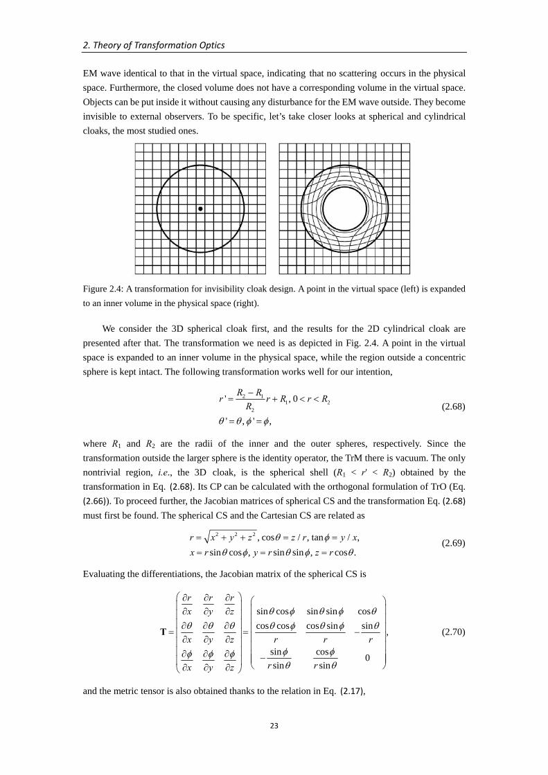
Figure 2.4: A transformation for invisibility cloak design. A point in the virtual space (left) is expanded to an inner volume in the physical space (right).

We consider the 3D spherical cloak first, and the results for the 2D cylindrical cloak are presented after that. The transformation we need is as depicted in Fig. 2.4. A point in the virtual space is expanded to an inner volume in the physical space, while the region outside a concentric sphere is kept intact. The following transformation works well for our intention,

2 1

1 22

' , 0

' , ' ,

R Rr r R r RR

θ θ φ φ

−= + < <

= = (2.68)

where R1 and R2 are the radii of the inner and the outer spheres, respectively. Since the transformation outside the larger sphere is the identity operator, the TrM there is vacuum. The only nontrivial region, i.e., the 3D cloak, is the spherical shell (R1 < r' < R2) obtained by the transformation in Eq. (2.68). Its CP can be calculated with the orthogonal formulation of TrO (Eq. (2.66)). To proceed further, the Jacobian matrices of spherical CS and the transformation Eq. (2.68) must first be found. The spherical CS and the Cartesian CS are related as

2 2 2 , cos / , tan / ,

sin cos , sin sin , cos .r x y z z r y xx r y r z r

θ φθ φ θ φ θ

= + + = =

= = = (2.69)

Evaluating the differentiations, the Jacobian matrix of the spherical CS is

sin cos sin sin coscos cos cos sin sin ,

sin cos 0sin sin

r r rx y z

x y z r r r

r rx y z

θ φ θ φ θθ θ θ θ φ θ φ θ

φ φφ φ φθ θ

⎛ ⎞∂ ∂ ∂ ⎛ ⎞⎜ ⎟ ⎜ ⎟∂ ∂ ∂⎜ ⎟ ⎜ ⎟⎜ ⎟∂ ∂ ∂ ⎜ ⎟= = −⎜ ⎟ ⎜ ⎟∂ ∂ ∂⎜ ⎟ ⎜ ⎟⎜ ⎟∂ ∂ ∂ ⎜ ⎟−⎜ ⎟⎜ ⎟ ⎝ ⎠∂ ∂ ∂⎝ ⎠

T (2.70)

and the metric tensor is also obtained thanks to the relation in Eq. (2.17),

2. Theory of Transformation Optics 

24 

12 2 2

1 11 .sin

T diagr r θ

− ⎛ ⎞= = ⎜ ⎟⎝ ⎠

g TT (2.71)

For the transformation Eq. (2.68), the Jacobian matrix is

2 1

2

1 1 .R R

diagR

⎛ ⎞−= ⎜ ⎟

⎝ ⎠λ (2.72)

Substitution of Eqs. (2.71) and (2.72) into Eq. (2.66) gives

1/2 1/2 2 1

2

' '' ,R R r rdiag

R r r− ⎛ ⎞−

= = ⎜ ⎟⎝ ⎠

S g λg (2.73)

and the CP of the spherical cloak

2

2 2 1

0 2 1 2

' 1 1 .'

R R R rdiagR R R rε

⎛ ⎞⎛ ⎞−⎜ ⎟= ⎜ ⎟⎜ ⎟− ⎝ ⎠⎝ ⎠

ε

The final result should only contain coordinate variables in the physical space. Eliminating the

radial variable r of the virtual space, we obtain

2

2 1

0 2 1

'' 1 1 .'

R r RdiagR R rε

⎛ ⎞−⎛ ⎞= ⎜ ⎟⎜ ⎟⎜ ⎟− ⎝ ⎠⎝ ⎠

ε (2.74)

For the 2D cylindrical cloak, the transformation with cylindrical coordinates (r, θ, z) is essentially the same as that for the spherical cloak

2 1

1 22

' , 0

' , ' .

R Rr r R r RRz zθ θ

−= + < <

= = (2.75)

The Jacobian matrix and the metric tensor become

cos sin 0sin cos 0 ,

0 0 1

r r rx y z

x y z r rz z zx y z

θ θθ θ θ θ θ

⎛ ⎞∂ ∂ ∂⎜ ⎟∂ ∂ ∂ ⎛ ⎞⎜ ⎟ ⎜ ⎟⎜ ⎟∂ ∂ ∂ ⎜ ⎟= = −⎜ ⎟ ⎜ ⎟∂ ∂ ∂⎜ ⎟ ⎜ ⎟⎜ ⎟∂ ∂ ∂ ⎝ ⎠⎜ ⎟∂ ∂ ∂⎝ ⎠

T (2.76)

12

11 1 .T diagr

− ⎛ ⎞= = ⎜ ⎟⎝ ⎠

g TT (2.77)

The Jacobian matrix of the transformation Eq. (2.75) is the same as Eq. (2.72). Insert Eqs. (2.72) and

(2.77) into Eq. (2.66),

1/2 1/2 2 1

2

'' 1R R rdiagR r

− ⎛ ⎞−= = ⎜ ⎟

⎝ ⎠S g λg (2.78)

and

2. Theory of Transformation Optics 

25 

2 2

2 2 1

0 2 1 2

' ' 1 .'

R R Rr rdiagR R r R rε

⎛ ⎞⎛ ⎞− ⎛ ⎞⎜ ⎟= ⎜ ⎟ ⎜ ⎟⎜ ⎟− ⎝ ⎠⎝ ⎠⎝ ⎠

ε

Eliminating the radial variable r, we get

2

1 2 1

0 1 2 1

' '' ' .' ' '

r R R r Rrdiagr r R R R rε

⎛ ⎞⎛ ⎞− −⎜ ⎟= ⎜ ⎟⎜ ⎟− −⎝ ⎠⎝ ⎠

ε (2.79)

Besides experimental verification, numerical simulation is a widely used and well accepted

technique to test theoretical ideas and designs. We would like to use numerical simulation to

illustrate the invisibility effect. The CP of the 2D cylindrical cloak enable the decoupling of

Transverse Electric (TE) and Transverse Magnetic (TM) excitations. In the 2D simulation, let’s take

the TM case as an example, whose field components include Hz, Ex and Ey. Accordingly, only the

axial component of the magnetic permeability and the transverse components of the electric

permittivity are required in the simulation. The finite element method (FEM) based commercial

software COMSOL [8] is applied as the simulation tool throughout the present thesis. In COMSOL,

the cylindrical components of the permittivity tensor can not be directly input for simulation yet. We

need the Cartesian components. The Cartesian permittivity tensor is transformed from that in

cylindrical components Eq. (2.79) with the formula in Eq. (2.67),

2 21 1

1 1

2 21 1

1 1

2

2 1

2 1

' ' ' '

' '' 'cos ' sin ' sin 'cos ' 0' ' ' '

' '' 'sin 'cos ' sin ' cos ' 0 .' ' ' '

'0 0'

T

r R r Rr rr r R r r R

r R r Rr rr r R r r R

R r RR R r

θ θ θ θ

θ θ θ θ

=

⎛ ⎞⎛ ⎞− −⎜ ⎟+ −⎜ ⎟− −⎜ ⎟⎝ ⎠⎜ ⎟⎛ ⎞− −⎜ ⎟= − +⎜ ⎟⎜ ⎟− −⎝ ⎠⎜ ⎟⎜ ⎟⎛ ⎞ −⎜ ⎟⎜ ⎟⎜ ⎟−⎝ ⎠⎝ ⎠

ε U ε U

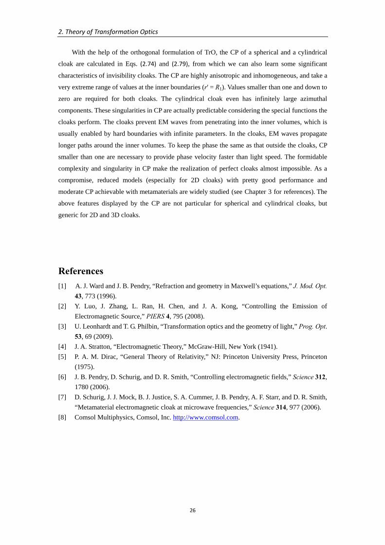
In Fig. 2.5, the numerical implementation of the Cartesian permittivity tensor provides the total

magnetic field distribution when a plane wave illuminates the cylindrical cloak. The invisibility

effect of the cylindrical cloak is clearly illustrated.

 

Figure 2.5: An EM plane wave propagates through a cylindrical invisibility cloak.  

2. Theory of Transformation Optics 

26 

With the help of the orthogonal formulation of TrO, the CP of a spherical and a cylindrical

cloak are calculated in Eqs. (2.74) and (2.79), from which we can also learn some significant

characteristics of invisibility cloaks. The CP are highly anisotropic and inhomogeneous, and take a

very extreme range of values at the inner boundaries (r' = R1). Values smaller than one and down to

zero are required for both cloaks. The cylindrical cloak even has infinitely large azimuthal

components. These singularities in CP are actually predictable considering the special functions the

cloaks perform. The cloaks prevent EM waves from penetrating into the inner volumes, which is

usually enabled by hard boundaries with infinite parameters. In the cloaks, EM waves propagate

longer paths around the inner volumes. To keep the phase the same as that outside the cloaks, CP

smaller than one are necessary to provide phase velocity faster than light speed. The formidable

complexity and singularity in CP make the realization of perfect cloaks almost impossible. As a

compromise, reduced models (especially for 2D cloaks) with pretty good performance and

moderate CP achievable with metamaterials are widely studied (see Chapter 3 for references). The

above features displayed by the CP are not particular for spherical and cylindrical cloaks, but

generic for 2D and 3D cloaks.

References [1] A. J. Ward and J. B. Pendry, “Refraction and geometry in Maxwell’s equations,” J. Mod. Opt.

43, 773 (1996). [2] Y. Luo, J. Zhang, L. Ran, H. Chen, and J. A. Kong, “Controlling the Emission of

Electromagnetic Source,” PIERS 4, 795 (2008). [3] U. Leonhardt and T. G. Philbin, “Transformation optics and the geometry of light,” Prog. Opt.

53, 69 (2009). [4] J. A. Stratton, “Electromagnetic Theory,” McGraw-Hill, New York (1941). [5] P. A. M. Dirac, “General Theory of Relativity,” NJ: Princeton University Press, Princeton

(1975). [6] J. B. Pendry, D. Schurig, and D. R. Smith, “Controlling electromagnetic fields,” Science 312,

1780 (2006). [7] D. Schurig, J. J. Mock, B. J. Justice, S. A. Cummer, J. B. Pendry, A. F. Starr, and D. R. Smith,

“Metamaterial electromagnetic cloak at microwave frequencies,” Science 314, 977 (2006). [8] Comsol Multiphysics, Comsol, Inc. http://www.comsol.com.

 

          27 

3. Reduced Two-dimensional Cloaks of Arbitrary Shapes

The idea of reduced models for 2D cloaks has already been mentioned in the previous chapter. It is

crucial for the practical realization and application of invisibility cloaks. In this chapter, we will first

give a brief introduction to reduced models and how they are designed. Thereafter a method of

designing reduced 2D cloaks of arbitrary shapes is proposed for the first time. Numerical

simulations for an elliptic and a bow-tie shaped cloak are carried out to demonstrate the

effectiveness of the method.

3.1 Reduced Cylindrical Cloaks

In the cylindrical cloak example in Section 2.4, we have already witnessed the singularity in its CP.

Near the inner boundary the radial and axial parameters are smaller than one, and become zero at the

boundary, while azimuthal components even become infinite at the inner boundary. These singular

behaviors make the realization of 2D perfect cloaks impossible. Taking advantage of metamaterials,

parameters less than one are feasible, but infinitely large parameters are still beyond reach. Without

infinities in the CP, 3D cloaks appear to be easier to realize. However, the anisotropy and

inhomogeneity in 3D structures pose huge difficulties for fabrication. As a compromise between

performance and the feasibility of experimental realization, reduced models for 2D cloaks free from

infinities in the CP can produce a good but not perfect invisibility effect. The first experimental

demonstration of a cloak [1] was actually constructed as a reduced 2D cloak.

In view of the high symmetry, the cylindrical cloak is the most studied 2D cloak. Almost all

studies of reduced models are about cylindrical cloaks. The general design strategy for most of them

is also specific to cylindrical cloaks. Considering TE polarized excitations, the EM wave behaviors

are completely described by the electric field component Ez, which follows the wave equation

202

1 1 1 0.z zz

z z r

E Er k Er r r rθε μ ε θ μ θ⎡ ⎤⎛ ⎞ ⎛ ⎞∂ ∂∂ ∂

+ + =⎢ ⎥⎜ ⎟ ⎜ ⎟∂ ∂ ∂ ∂⎢ ⎥ ⎝ ⎠⎝ ⎠⎣ ⎦ (3.1)

In the design strategy, we make the approximate assumption of radially invariant μθ whereby Eq.

(3.1) becomes

2 2

202 2 2

1 1 1 1 1 0.z z zz

z z z r

E E E k Er r r rθ θε μ ε μ ε μ θ

∂ ∂ ∂+ + + =

∂ ∂ ∂ (3.2)

Though not accurate, Eq. (3.2) does provide a guide for designing reduced cloaks to certain extent.

The products εzμθ and εzμr specify Eq. (3.2) completely. As long as the products for reduced cloaks

are kept the same as those for perfect cloaks, we can expect similar EM wave behaviors as in the

case of perfect invisibility. The two products for the perfect cylindrical cloak designed in Section

3. Reduced Two‐dimensional Cloaks of Arbitrary Shapes 

28 

2.4 are

2 2 2

2 2 1

0 0 2 1 0 0 2 1

, .z z rR R r RR R R R r

θε μ ε με μ ε μ

⎛ ⎞ ⎛ ⎞ −⎛ ⎞= =⎜ ⎟ ⎜ ⎟ ⎜ ⎟− − ⎝ ⎠⎝ ⎠ ⎝ ⎠ (3.3)

Manipulation of the three parameters helps to avoid the singularity in the CP and keep the products

unchanged at the same time. In [1], the first reduced model has the CP

2 2

2 1

0 2 1 0 0

, , 1,z rR r RR R r

θμε με μ μ

⎛ ⎞ −⎛ ⎞= = =⎜ ⎟ ⎜ ⎟− ⎝ ⎠⎝ ⎠ (3.4)

which fulfill Eq. (3.3) and are free of infinite parameters. For the TM polarization case, another set of products similar to that in Eq. (3.3) is used. In [2], a non-magnetic reduced cloak, supposed to work at visible frequencies, has the CP

2 22

2 1 2

0 0 2 1 0 2 1

1, , .z r R r R RR R r R R

θεμ εμ ε ε

⎛ ⎞ ⎛ ⎞−⎛ ⎞= = =⎜ ⎟ ⎜ ⎟⎜ ⎟− −⎝ ⎠⎝ ⎠ ⎝ ⎠ (3.5)

Later an impedance matched reduced model [3] was proposed to suppress strong scattering due to outer boundary reflection,

2

2 1 2 2

0 2 1 0 2 1 0 2 1

, , .z rR r R R RR R r R R R R

θμε με μ μ

−⎛ ⎞= = =⎜ ⎟− − −⎝ ⎠ (3.6)

It also has the same products as in Eq. (3.3).

Apart from this most used strategy, another more systematic study on designing reduced

cylindrical cloaks was reported in [4]. The method introduces a series expansion to represent μθ of a

perfect cloak. Then reduced models are obtained when taking different truncation orders in the

expansion. The lowest order result is exactly the same as the previously discussed strategy. It will

get closer to the perfect cloak when more terms are included.

3.2 Reduced Two-dimensional Cloaks of Arbitrary Shapes Although reduced models for 2D cloaks are widely investigated as discussed in the introduction,

almost all research concentrates on cylindrical cloaks. For arbitrarily shaped cloaks, only perfect

models are developed with TrO in the literature. The experimental realization, however, must be

assisted by corresponding reduced models. In this section, we propose a general method to design

reduced models for 2D cloaks of arbitrary shapes. The description of the general guideline is

followed by two concrete examples of reduced models, an elliptic and a bow-tie shaped cloak.

Prominent cloaking effects are observed in numerical demonstrations.

As noticed in reduced cylindrical cloaks, the singularity removed by reduced models is the

infinity in the CP. In this sense, 3D perfect cloaks are non-singular. It is thus natural to take

advantage of this non-singular nature of 3D perfect cloaks to construct CP for reduced 2D cloaks.

Consider a 3D perfect cloak with mirror symmetry. When this cloak is illuminated by a plane wave

with its wave vector parallel to the symmetry plane, the plane wave has the Poynting vector on the

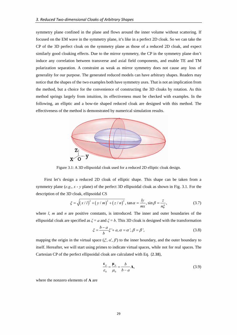
3. Reduced Two‐dimensional Cloaks of Arbitrary Shapes 

29 

symmetry plane confined in the plane and flows around the inner volume without scattering. If

focused on the EM wave in the symmetry plane, it’s like in a perfect 2D cloak. So we can take the

CP of the 3D perfect cloak on the symmetry plane as those of a reduced 2D cloak, and expect

similarly good cloaking effects. Due to the mirror symmetry, the CP in the symmetry plane don’t

induce any correlation between transverse and axial field components, and enable TE and TM

polarization separation. A constraint as weak as mirror symmetry does not cause any loss of

generality for our purpose. The generated reduced models can have arbitrary shapes. Readers may

notice that the shapes of the two examples both have symmetry axes. That is not an implication from

the method, but a choice for the convenience of constructing the 3D cloaks by rotation. As this

method springs largely from intuition, its effectiveness must be checked with examples. In the

following, an elliptic and a bow-tie shaped reduced cloak are designed with this method. The

effectiveness of the method is demonstrated by numerical simulation results.

Figure 3.1: A 3D ellipsoidal cloak used for a reduced 2D elliptic cloak design.

First let’s design a reduced 2D cloak of elliptic shape. This shape can be taken from a

symmetry plane (e.g., x - y plane) of the perfect 3D ellipsoidal cloak as shown in Fig. 3.1. For the

description of the 3D cloak, ellipsoidal CS

( ) ( ) ( )2 2 2/ / / , tan , sin ,ly zx l y m z nmx n

ξ α βξ

= + + = = (3.7)

where l, m and n are positive constants, is introduced. The inner and outer boundaries of the

ellipsoidal cloak are specified as ξ = a and ξ = b. This 3D cloak is designed with the transformation

' , ', ',b a ab

ξ ξ α α β β−= + = = (3.8)

mapping the origin in the virtual space (ξ', α', β') to the inner boundary, and the outer boundary to

itself. Hereafter, we will start using primes to indicate virtual spaces, while not for real spaces. The

Cartesian CP of the perfect ellipsoidal cloak are calculated with Eq. (2.38),

0 0

,p p bb aε μ

= =−

ε μA (3.9)

where the nonzero elements of A are

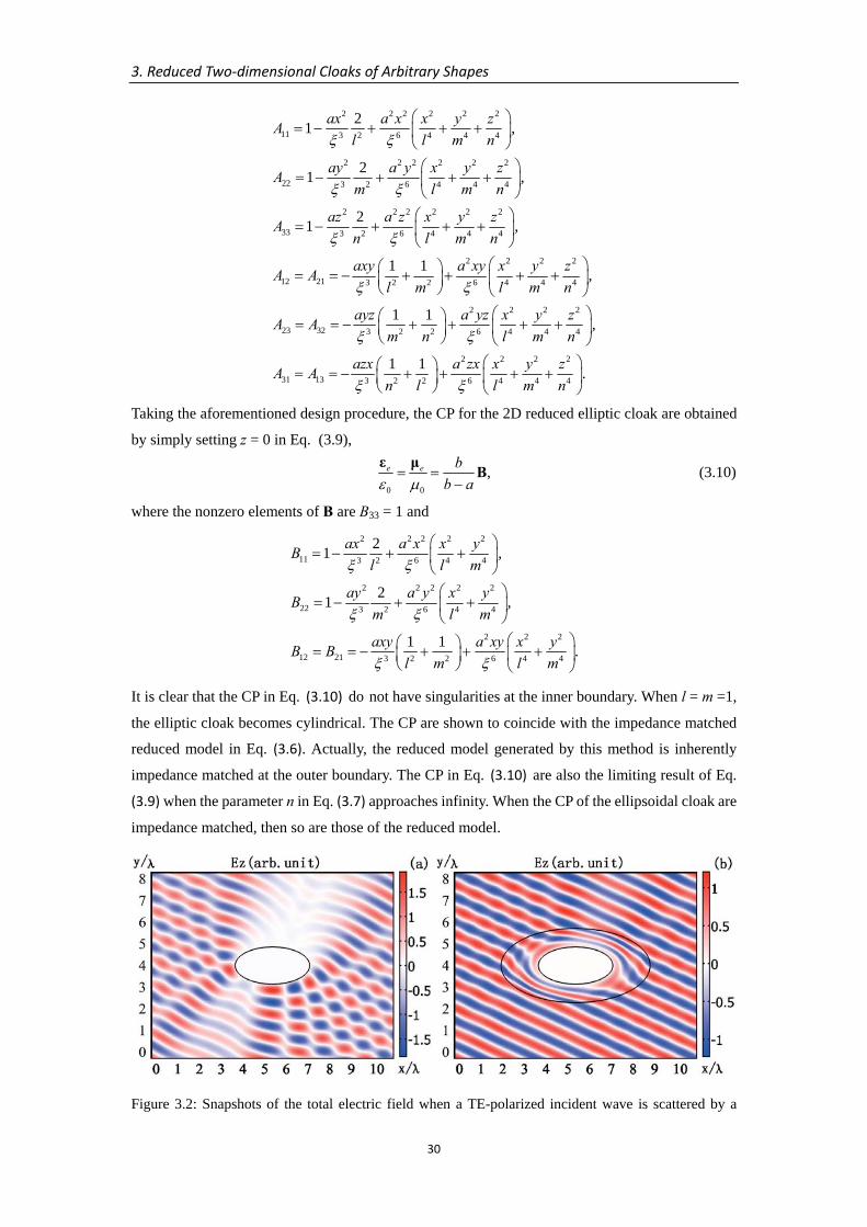
3. Reduced Two‐dimensional Cloaks of Arbitrary Shapes 

30 

2 2 2 2 2 2

11 3 2 6 4 4 4

2 2 2 2 2 2

22 3 2 6 4 4 4

2 2 2 2 2 2

33 3 2 6 4 4 4

2 2 2 2

12 21 3 2 2 6 4 4 4

23 32 3 2

21 ,

21 ,

21 ,

1 1 ,

1 1

ax a x x y zAl l m n

ay a y x y zAm l m n

az a z x y zAn l m n

axy a xy x y zA Al m l m n

ayzA Am

ξ ξ

ξ ξ

ξ ξ

ξ ξ

ξ

⎛ ⎞= − + + +⎜ ⎟

⎝ ⎠⎛ ⎞

= − + + +⎜ ⎟⎝ ⎠⎛ ⎞

= − + + +⎜ ⎟⎝ ⎠

⎛ ⎞⎛ ⎞= = − + + + +⎜ ⎟⎜ ⎟⎝ ⎠ ⎝ ⎠

= = − +2 2 2 2

2 6 4 4 4

2 2 2 2

31 13 3 2 2 6 4 4 4

,

1 1 .

a yz x y zn l m n

azx a zx x y zA An l l m n

ξ

ξ ξ

⎛ ⎞⎛ ⎞ + + +⎜ ⎟⎜ ⎟⎝ ⎠ ⎝ ⎠

⎛ ⎞⎛ ⎞= = − + + + +⎜ ⎟⎜ ⎟⎝ ⎠ ⎝ ⎠

Taking the aforementioned design procedure, the CP for the 2D reduced elliptic cloak are obtained

by simply setting z = 0 in Eq. (3.9),

0 0

,e e bb aε μ

= =−

ε μB (3.10)

where the nonzero elements of B are B33 = 1 and

2 2 2 2 2

11 3 2 6 4 4

2 2 2 2 2

22 3 2 6 4 4

2 2 2

12 21 3 2 2 6 4 4

21 ,

21 ,

1 1 .

ax a x x yBl l m

ay a y x yBm l m

axy a xy x yB Bl m l m

ξ ξ

ξ ξ

ξ ξ

⎛ ⎞= − + +⎜ ⎟

⎝ ⎠⎛ ⎞

= − + +⎜ ⎟⎝ ⎠

⎛ ⎞⎛ ⎞= = − + + +⎜ ⎟⎜ ⎟⎝ ⎠ ⎝ ⎠

It is clear that the CP in Eq. (3.10) do not have singularities at the inner boundary. When l = m =1,

the elliptic cloak becomes cylindrical. The CP are shown to coincide with the impedance matched

reduced model in Eq. (3.6). Actually, the reduced model generated by this method is inherently

impedance matched at the outer boundary. The CP in Eq. (3.10) are also the limiting result of Eq.

(3.9) when the parameter n in Eq. (3.7) approaches infinity. When the CP of the ellipsoidal cloak are

impedance matched, then so are those of the reduced model.

Figure 3.2: Snapshots of the total electric field when a TE-polarized incident wave is scattered by a

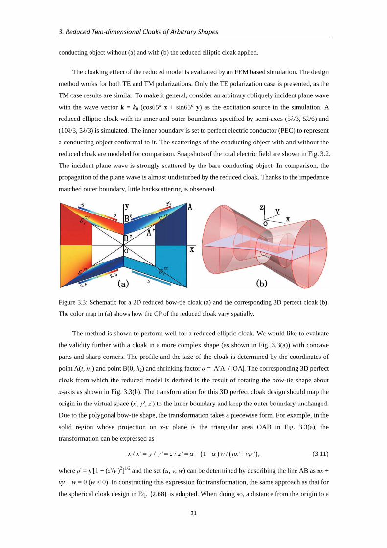
3. Reduced Two‐dimensional Cloaks of Arbitrary Shapes 

31 

conducting object without (a) and with (b) the reduced elliptic cloak applied.

The cloaking effect of the reduced model is evaluated by an FEM based simulation. The design

method works for both TE and TM polarizations. Only the TE polarization case is presented, as the

TM case results are similar. To make it general, consider an arbitrary obliquely incident plane wave

with the wave vector k = k0 (cos65° x + sin65° y) as the excitation source in the simulation. A

reduced elliptic cloak with its inner and outer boundaries specified by semi-axes (5λ/3, 5λ/6) and

(10λ/3, 5λ/3) is simulated. The inner boundary is set to perfect electric conductor (PEC) to represent

a conducting object conformal to it. The scatterings of the conducting object with and without the

reduced cloak are modeled for comparison. Snapshots of the total electric field are shown in Fig. 3.2.

The incident plane wave is strongly scattered by the bare conducting object. In comparison, the

propagation of the plane wave is almost undisturbed by the reduced cloak. Thanks to the impedance

matched outer boundary, little backscattering is observed.

Figure 3.3: Schematic for a 2D reduced bow-tie cloak (a) and the corresponding 3D perfect cloak (b).

The color map in (a) shows how the CP of the reduced cloak vary spatially.

The method is shown to perform well for a reduced elliptic cloak. We would like to evaluate

the validity further with a cloak in a more complex shape (as shown in Fig. 3.3(a)) with concave

parts and sharp corners. The profile and the size of the cloak is determined by the coordinates of

point A(t, h1) and point B(0, h2) and shrinking factor α = |A’A| / |OA|. The corresponding 3D perfect

cloak from which the reduced model is derived is the result of rotating the bow-tie shape about

x-axis as shown in Fig. 3.3(b). The transformation for this 3D perfect cloak design should map the

origin in the virtual space (x', y', z') to the inner boundary and keep the outer boundary unchanged.

Due to the polygonal bow-tie shape, the transformation takes a piecewise form. For example, in the

solid region whose projection on x-y plane is the triangular area OAB in Fig. 3.3(a), the

transformation can be expressed as

( ) ( )/ ' / ' / ' 1 / ' ' ,x x y y z z w ux vα α ρ= = = − − + (3.11)

where ρ' = y'[1 + (z'/y')2]1/2 and the set (u, v, w) can be determined by describing the line AB as ux +

vy + w = 0 (w < 0). In constructing this expression for transformation, the same approach as that for

the spherical cloak design in Eq. (2.68) is adopted. When doing so, a distance from the origin to a

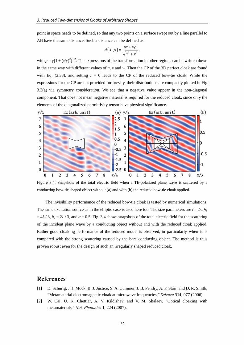
3. Reduced Two‐dimensional Cloaks of Arbitrary Shapes 

32 

point in space needs to be defined, so that any two points on a surface swept out by a line parallel to

AB have the same distance. Such a distance can be defined as

( )2 2

, ,ux vd xu v

ρρ +=

+

with ρ = y[1 + (z/y)2]1/2. The expressions of the transformation in other regions can be written down

in the same way with different values of u, v and w. Then the CP of the 3D perfect cloak are found

with Eq. (2.38), and setting z = 0 leads to the CP of the reduced bow-tie cloak. While the

expressions for the CP are not provided for brevity, their distributions are compactly plotted in Fig.

3.3(a) via symmetry consideration. We see that a negative value appear in the non-diagonal

component. That does not mean negative material is required for the reduced cloak, since only the

elements of the diagonalized permittivity tensor have physical significance.

Figure 3.4: Snapshots of the total electric field when a TE-polarized plane wave is scattered by a

conducting bow-tie shaped object without (a) and with (b) the reduced bow-tie cloak applied.

The invisibility performance of the reduced bow-tie cloak is tested by numerical simulations.

The same excitation source as in the elliptic case is used here too. The size parameters are t = 2λ, h1

= 4λ / 3, h2 = 2λ / 3, and α = 0.5. Fig. 3.4 shows snapshots of the total electric field for the scattering

of the incident plane wave by a conducting object without and with the reduced cloak applied.

Rather good cloaking performance of the reduced model is observed, in particularly when it is

compared with the strong scattering caused by the bare conducting object. The method is thus

proven robust even for the design of such an irregularly shaped reduced cloak.

References [1] D. Schurig, J. J. Mock, B. J. Justice, S. A. Cummer, J. B. Pendry, A. F. Starr, and D. R. Smith,

“Metamaterial electromagnetic cloak at microwave frequencies,” Science 314, 977 (2006). [2] W. Cai, U. K. Chettiar, A. V. Kildishev, and V. M. Shalaev, “Optical cloaking with

metamaterials,” Nat. Photonics 1, 224 (2007).

3. Reduced Two‐dimensional Cloaks of Arbitrary Shapes 

33 

[3] M. Yan, Z. Ruan, and M. Qiu, “Scattering characteristics of simplified cylindrical invisibility cloaks,” Opt. Express 15, 17772 (2007).

[4] P. Collins and J. McGuirk, “A novel methodology for deriving improved material parameter sets for simplified cylindrical cloaks,” J. Opt. A 11, 015104 (2009).

3. Reduced Two‐dimensional Cloaks of Arbitrary Shapes 

34 

 

35 

4. Inverse Transformation Optics and its Applications

In this chapter, we introduce a technique for reversing the procedure of TrO, which is called inverse

transformation optics hereafter. The general idea of inverse TrO is discussed in the first section.

Then the technique is applied to analyze the reflection for 2D finite-embedded coordinate

transformations.

4.1 Inverse Transformation Optics

When TrO is applied to a device design, given a virtual space with known material specifications

(usually vacuous or isotropic) and a transformation to the real space, the TrM or the designed device

can then be determined. As seen from the formulae in Eqs. (2.38) and (2.39), TrM are generally

anisotropic and inhomogeneous, much more complex than the original media before transformation.

What do we have if the procedure is reversed? Given an anisotropic and perhaps inhomogeneous

medium distribution, we need to find a transformation and transform the anisotropic medium back

to an isotropic medium in a virtual space. Since isotropic media are considerably easier to deal with,

this inverse TrO can be utilized to help treat problems involving anisotropic and inhomogeneous

medium distribution. Once a proper transformation relation is established, the problems are

transformed to simpler ones in the virtual space containing isotropic media. The simplified

problems can then hopefully be solved with a smaller effort. Results for the original problems are

finally obtained from the results for the simplified problems by standard TrO procedures.

To explore the feasibility of this idea, consider the CP of the TrM in Eq. (2.38)

( )1' det ,Tε −=ε Λ Λ Λ (4.1)

where the permittivity of the original medium in the virtual space is assumed to be isotropic,

represented by a scalar ε'. For the inverse TrO, the anisotropic and inhomogeneous medium

specified by ε is known. We are looking for some transformation characteristic of its Jacobian

matrix Λ, so that an isotropic medium is obtained

( ) ( )1 1' det .T

ε − −= Λ ε Λ Λ (4.2)

For an ordinary lossless medium, the permittivity tensor is Hermitian [1] and positive definite.

Assume for simplicity the case of a real tensor ε for the current development. The scalar ε' is just an

identity matrix. As long as the general symmetric matrix ε can be decomposed as

( )1 2 3, , ,Tdiag ε ε ε=ε Q Q (4.3)

the Jacobian matrix is formally found to be

( )1 2 3, , ,diag ε ε ε=Λ Q (4.4)

4. Inverse Transformation Optics and its Applications 

36 

and the isotropic medium in Eq. (4.2) turns out to be

( )1 2 3' det .ε ε ε ε= Q (4.5)

Eq. (4.3) is simply the eigen-decomposition of ε [2], which is available for any symmetric matrix.

Thus, in principle inverse TrO is applicable for any anisotropic medium with a symmetric

permittivity tensor. One may note that the diagonalization process essentially corresponds to

finding the principal axes of the anisotropic medium. However, the theory of TrO enables the

treatment of the spatially inhomogeneous medium distribution at the same time. The decomposition

in Eq. (4.3) is not unique, meaning that we have additional flexibility to play with. Auxiliary

conditions can be imposed on transformations for special applications, as will be seen in the

reflection analysis example.

In TrO, the formulas for permittivity and permeability of TrM (Eqs. (2.38) and (2.39)) have

the same form due to the duality of the EM theory. An inverse transformation giving isotropy in

permittivity is thus not guaranteed to simultaneously give isotropy in permeability. It is therefore

not possible for inverse TrO to produce an isotropic medium from a general anisotropic medium

with anisotropy in both permittivity and permeability. Fortunately, in most applications we don’t

have such kind of general anisotropic media. For 2D problems, e.g., the example we are about to

discuss, TE and TM polarization states can be considered separately. This issue of correlation does

not exist.

4.2 Reflection Analysis for 2D Finite-Embedded Coordinate

Transformation

In TrO, the transformation between two spaces is assumed to apply for the whole domain in

spaces. The TrM specification is also for the whole physical space. If the transformation is

nontrivial even when extended into infinity, the realization of such a TrM would be an impossible

mission. For the case of invisibility cloaks, the transformation is the identity operator outside a

certain finite region. The TrM is different from vacuum only in the finite region. According to this

argument, the transformation has to be the identity outside a finite region so that the TrM can be

realized. In consequence, the TrM can only allow for local manipulation of EM waves. To break this

severe limitation, the functional and nontrivial transformation is assumed to be embedded in a finite

region for device design [3]. TrO is only applied in the finite region, i.e., within the device. This

scheme is called Finite Embedded Coordinate Transformation (FECT). In [3] where FECT is

proposed, a beam shifter and a beam splitter are presented for the sake of example. After FECT was

introduced, ensuing research on device designs with FECT has been extensively conducted [4-8].

From a theoretical point of view, FECT is not totally consistent with TrO, where the whole

domain is transformed. The performance of a device design by FECT can not be completely

described by TrO, especially with respect to boundaries. The non-transformed outer region can be

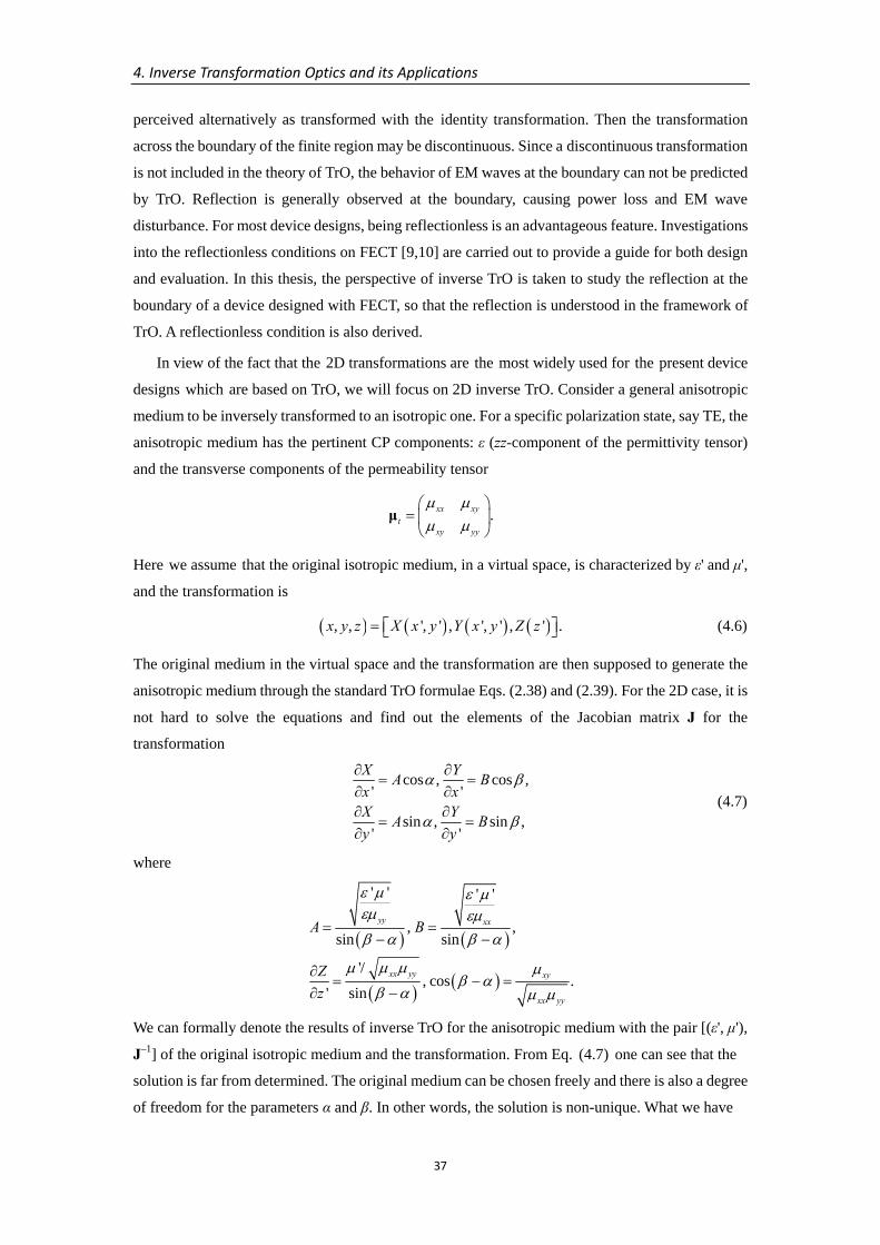
4. Inverse Transformation Optics and its Applications 

37 

perceived alternatively as transformed with the identity transformation. Then the transformation

across the boundary of the finite region may be discontinuous. Since a discontinuous transformation

is not included in the theory of TrO, the behavior of EM waves at the boundary can not be predicted

by TrO. Reflection is generally observed at the boundary, causing power loss and EM wave

disturbance. For most device designs, being reflectionless is an advantageous feature. Investigations

into the reflectionless conditions on FECT [9,10] are carried out to provide a guide for both design

and evaluation. In this thesis, the perspective of inverse TrO is taken to study the reflection at the

boundary of a device designed with FECT, so that the reflection is understood in the framework of

TrO. A reflectionless condition is also derived.

In view of the fact that the 2D transformations are the most widely used for the present device

designs which are based on TrO, we will focus on 2D inverse TrO. Consider a general anisotropic

medium to be inversely transformed to an isotropic one. For a specific polarization state, say TE, the

anisotropic medium has the pertinent CP components: ε (zz-component of the permittivity tensor)

and the transverse components of the permeability tensor

.xx xyt

xy yy

μ μμ μ⎛ ⎞

= ⎜ ⎟⎝ ⎠

μ

Here we assume that the original isotropic medium, in a virtual space, is characterized by ε' and μ',

and the transformation is

( ) ( ) ( ) ( ), , ', ' , ', ' , ' .x y z X x y Y x y Z z= ⎡ ⎤⎣ ⎦ (4.6)

The original medium in the virtual space and the transformation are then supposed to generate the

anisotropic medium through the standard TrO formulae Eqs. (2.38) and (2.39). For the 2D case, it is

not hard to solve the equations and find out the elements of the Jacobian matrix J for the

transformation

cos , cos ,

' '

sin , sin ,' '

X YA Bx xX YA By y

α β

α β

∂ ∂= =

∂ ∂∂ ∂

= =∂ ∂

(4.7)

where

( ) ( )

( ) ( )

' ' ' '

, ,sin sin

'/, cos .

' sin

yy xx

xx yy xy

xx yy

A B

Zz

ε μ ε μεμ εμβ α β α

μ μ μ μβ α

β α μ μ

= =− −

∂= − =

∂ −

We can formally denote the results of inverse TrO for the anisotropic medium with the pair [(ε', μ'),

J–1] of the original isotropic medium and the transformation. From Eq. (4.7) one can see that the

solution is far from determined. The original medium can be chosen freely and there is also a degree

of freedom for the parameters α and β. In other words, the solution is non-unique. What we have

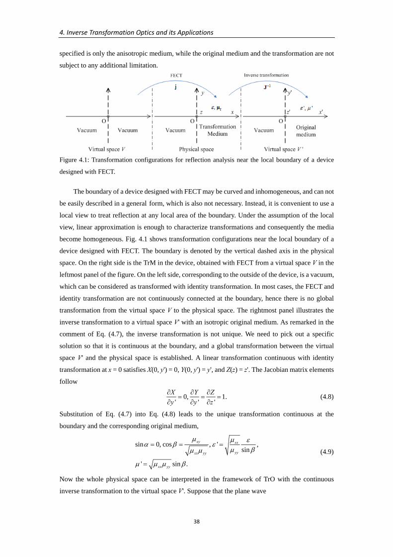
4. Inverse Transformation Optics and its Applications 

38 

specified is only the anisotropic medium, while the original medium and the transformation are not

subject to any additional limitation.

Figure 4.1: Transformation configurations for reflection analysis near the local boundary of a device

designed with FECT.

The boundary of a device designed with FECT may be curved and inhomogeneous, and can not

be easily described in a general form, which is also not necessary. Instead, it is convenient to use a

local view to treat reflection at any local area of the boundary. Under the assumption of the local

view, linear approximation is enough to characterize transformations and consequently the media

become homogeneous. Fig. 4.1 shows transformation configurations near the local boundary of a

device designed with FECT. The boundary is denoted by the vertical dashed axis in the physical

space. On the right side is the TrM in the device, obtained with FECT from a virtual space V in the

leftmost panel of the figure. On the left side, corresponding to the outside of the device, is a vacuum,

which can be considered as transformed with identity transformation. In most cases, the FECT and

identity transformation are not continuously connected at the boundary, hence there is no global

transformation from the virtual space V to the physical space. The rightmost panel illustrates the

inverse transformation to a virtual space V' with an isotropic original medium. As remarked in the

comment of Eq. (4.7), the inverse transformation is not unique. We need to pick out a specific

solution so that it is continuous at the boundary, and a global transformation between the virtual

space V' and the physical space is established. A linear transformation continuous with identity

transformation at x = 0 satisfies X(0, y') = 0, Y(0, y') = y', and Z(z) = z'. The Jacobian matrix elements

follow

0, 1.' ' '

X Y Zy y z∂ ∂ ∂

= = =∂ ∂ ∂

(4.8)

Substitution of Eq. (4.7) into Eq. (4.8) leads to the unique transformation continuous at the

boundary and the corresponding original medium,

sin 0, cos , ' ,

sin

' sin .

xy xx

yyxx yy

xx yy

μ μ εα β εμ βμ μ

μ μ μ β

= = =

=

(4.9)

Now the whole physical space can be interpreted in the framework of TrO with the continuous

inverse transformation to the virtual space V'. Suppose that the plane wave

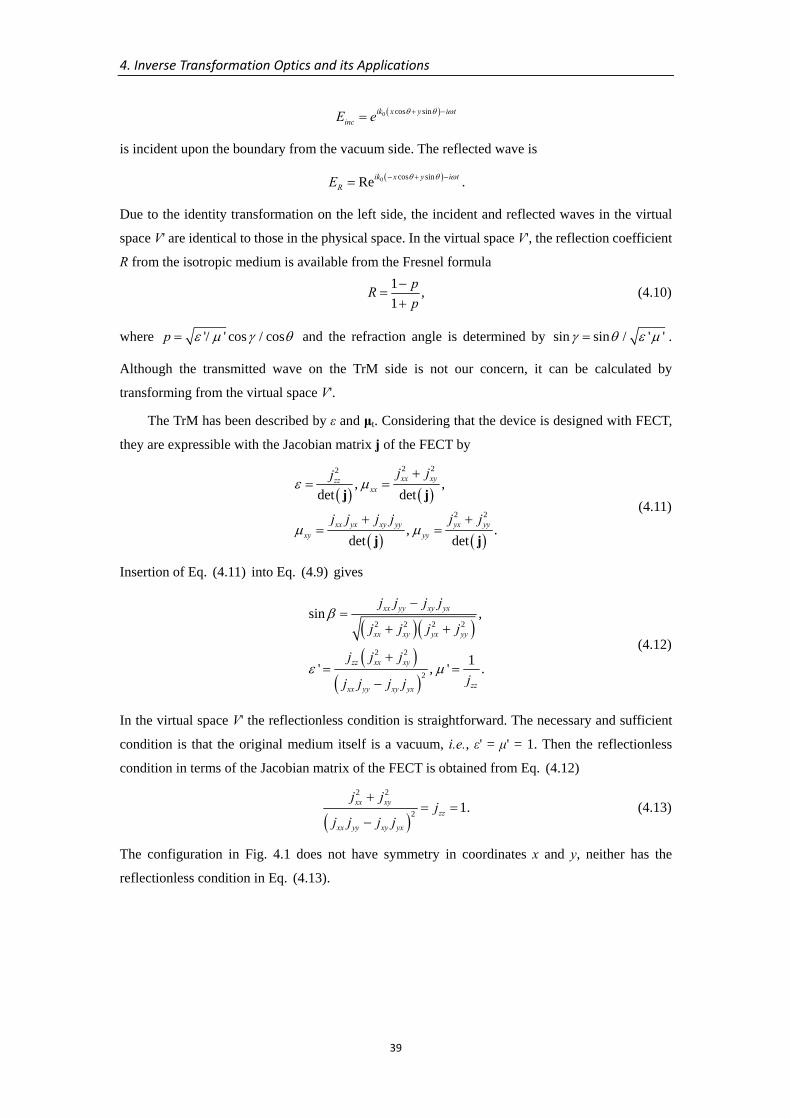
4. Inverse Transformation Optics and its Applications 

39 

( )0 cos sinik x y i tincE e θ θ ω+ −=

is incident upon the boundary from the vacuum side. The reflected wave is

( )0 cos sinRe .ik x y i tRE θ θ ω− + −=

Due to the identity transformation on the left side, the incident and reflected waves in the virtual

space V' are identical to those in the physical space. In the virtual space V', the reflection coefficient

R from the isotropic medium is available from the Fresnel formula

1 ,1

pRp

−=

+ (4.10)

where '/ ' cos / cosp ε μ γ θ= and the refraction angle is determined by sin sin / ' 'γ θ ε μ= .

Although the transmitted wave on the TrM side is not our concern, it can be calculated by

transforming from the virtual space V'.

The TrM has been described by ε and μt. Considering that the device is designed with FECT,

they are expressible with the Jacobian matrix j of the FECT by

( ) ( )

( ) ( )

2 22

2 2

, ,det det

, .det det

xx xyzzxx

xx yx xy yy yx yyxy yy

j jj

j j j j j j

ε μ

μ μ

+= =

+ += =

j j

j j

(4.11)

Insertion of Eq. (4.11) into Eq. (4.9) gives

( )( )( )

( )

2 2 2 2

2 2

2

sin ,

1' , ' .

xx yy xy yx

xx xy yx yy

zz xx xy

zzxx yy xy yx

j j j j

j j j j

j j j

jj j j j

β

ε μ

−=

+ +

+= =

−

(4.12)

In the virtual space V' the reflectionless condition is straightforward. The necessary and sufficient

condition is that the original medium itself is a vacuum, i.e., ε' = μ' = 1. Then the reflectionless

condition in terms of the Jacobian matrix of the FECT is obtained from Eq. (4.12)

( )

2 2

2 1.xx xyzz

xx yy xy yx

j jj

j j j j

+= =

− (4.13)

The configuration in Fig. 4.1 does not have symmetry in coordinates x and y, neither has the

reflectionless condition in Eq. (4.13).

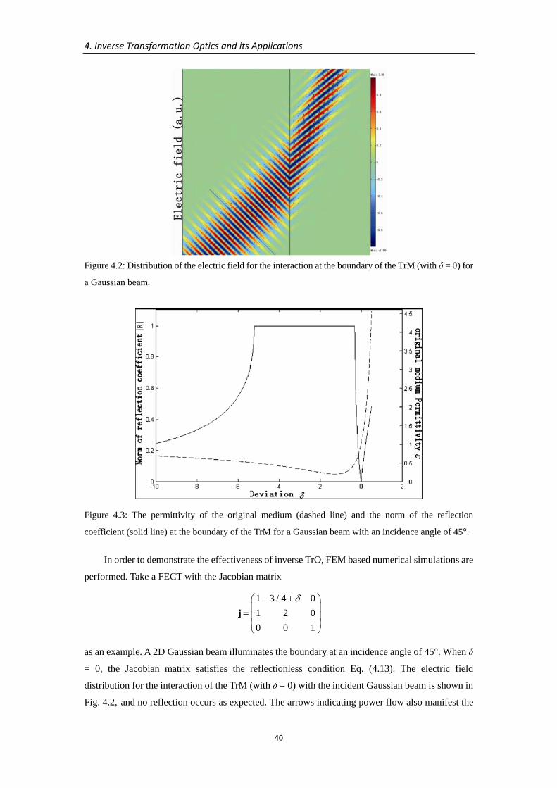
4. Inverse Transformation Optics and its Applications 

40 

Figure 4.2: Distribution of the electric field for the interaction at the boundary of the TrM (with δ = 0) for

a Gaussian beam.

Figure 4.3: The permittivity of the original medium (dashed line) and the norm of the reflection

coefficient (solid line) at the boundary of the TrM for a Gaussian beam with an incidence angle of 45°.

In order to demonstrate the effectiveness of inverse TrO, FEM based numerical simulations are

performed. Take a FECT with the Jacobian matrix

1 3 / 4 01 2 00 0 1

δ+⎛ ⎞⎜ ⎟= ⎜ ⎟⎜ ⎟⎝ ⎠

j

as an example. A 2D Gaussian beam illuminates the boundary at an incidence angle of 45°. When δ

= 0, the Jacobian matrix satisfies the reflectionless condition Eq. (4.13). The electric field

distribution for the interaction of the TrM (with δ = 0) with the incident Gaussian beam is shown in

Fig. 4.2, and no reflection occurs as expected. The arrows indicating power flow also manifest the

4. Inverse Transformation Optics and its Applications 

41 

total transmission. For situations with nonzero reflection, the original medium and the reflection

coefficient are accessible with Eqs. (4.12) and (4.10). They are plotted in Fig. 4.3 with δ in the range

of [–10, 5/4) (the permeability is constant 1). The reflection coefficient can be well understood with

the help of the permittivity of the original medium.

Besides the present application example, we notice that in [11] the authors essentially utilize

the same idea of inverse TrO to transform a reduced cloak (anisotropic) to an isotropic original

medium in a virtual space. The properties of reduced cloaks are thus simplified to those of

isotropic structures.

References [1] J. A. Kong, “Theory of Electromagnetic Waves,” Wiley, New York (1975). [2] http://en.wikipedia.org/wiki/Eigendecomposition_of_a_matrix [3] M. Rahm, S. A. Cummer, D. Schurig, J. B. Pendry, and D. R. Smith, “Optical design of

reflectionless complex media by finite embedded coordinate transformations,” Phys. Rev. Lett. 100, 063903 (2008).

[4] M. Rahm, D. A. Roberts, J. B. Pendry, and D. R. Smith, “Transformation-optical design of adaptive beam bends and beam expanders,” Opt. Express 16, 11555 (2008).

[5] D. H. Kwon and D. H. Werner, “Transformation optical designs for wave collimators, flat lenses, and right-angle bends,” New J. Phys. 10, 115012 (2008).

[6] W. X. Jiang, T. J. Cui, H. F. Ma, X. Y. Zhou, and Q. Cheng, “Cylindrical-to-plane-wave conversion via embedded optical transformation,” Appl. Phys. Lett. 92, 261903 (2008).

[7] H. Ma, S. B. Qu, Z. Xu, and J. F. Wang, “Wave-shape-keeping media,” Opt. Lett. 34, 127 (2009).

[8] T. R. Zhai, Y. Zhou, J. Zhou, and D. H. Liu, “Polarization controller based on embedded optical transformation,” Opt. Express 17, 17206 (2009).

[9] W. Yan, M. Yan, and M. Qiu, “Necessary and sufficient conditions for reflectionless transformation media in an isotropic and homogenous background,” arXiv:0806.3231v1, (2008).

[10] L. Bergamin, “Electromagnetic fields and boundary conditions at the interface ofgeneralized transformation media,” Phys. Rev. A 80, 063835 (2009).

[11] H. Y. Chen, J. Ng, C. W. Lee, Y. Lai, and C. T. Chan, “General Transformation for the Reduced Invisibility Cloak,” Phys. Rev. B 80, 085112 (2009).

4. Inverse Transformation Optics and its Applications 

42 

 

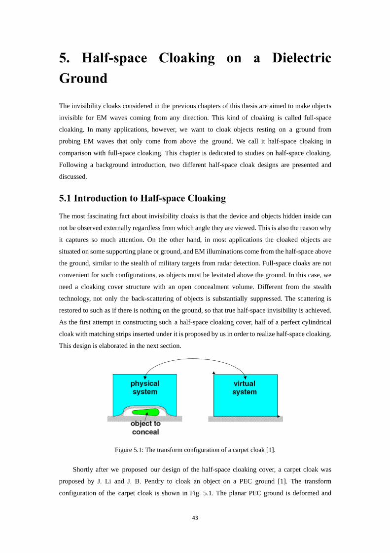
43 

5. Half-space Cloaking on a Dielectric Ground

The invisibility cloaks considered in the previous chapters of this thesis are aimed to make objects

invisible for EM waves coming from any direction. This kind of cloaking is called full-space

cloaking. In many applications, however, we want to cloak objects resting on a ground from

probing EM waves that only come from above the ground. We call it half-space cloaking in

comparison with full-space cloaking. This chapter is dedicated to studies on half-space cloaking.

Following a background introduction, two different half-space cloak designs are presented and

discussed.

5.1 Introduction to Half-space Cloaking

The most fascinating fact about invisibility cloaks is that the device and objects hidden inside can

not be observed externally regardless from which angle they are viewed. This is also the reason why

it captures so much attention. On the other hand, in most applications the cloaked objects are

situated on some supporting plane or ground, and EM illuminations come from the half-space above

the ground, similar to the stealth of military targets from radar detection. Full-space cloaks are not

convenient for such configurations, as objects must be levitated above the ground. In this case, we

need a cloaking cover structure with an open concealment volume. Different from the stealth

technology, not only the back-scattering of objects is substantially suppressed. The scattering is

restored to such as if there is nothing on the ground, so that true half-space invisibility is achieved.

As the first attempt in constructing such a half-space cloaking cover, half of a perfect cylindrical

cloak with matching strips inserted under it is proposed by us in order to realize half-space cloaking.

This design is elaborated in the next section.

Figure 5.1: The transform configuration of a carpet cloak [1].

Shortly after we proposed our design of the half-space cloaking cover, a carpet cloak was

proposed by J. Li and J. B. Pendry to cloak an object on a PEC ground [1]. The transform

configuration of the carpet cloak is shown in Fig. 5.1. The planar PEC ground is deformed and

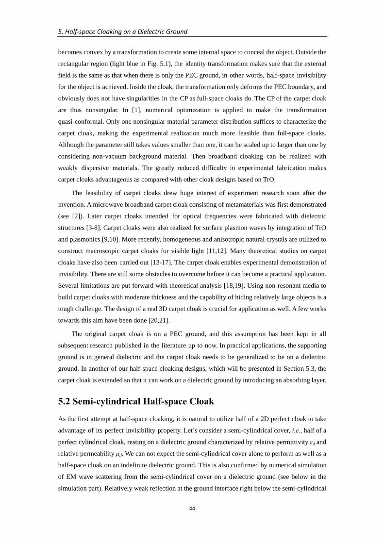
5. Half‐space Cloaking on a Dielectric Ground 

44 

becomes convex by a transformation to create some internal space to conceal the object. Outside the

rectangular region (light blue in Fig. 5.1), the identity transformation makes sure that the external

field is the same as that when there is only the PEC ground, in other words, half-space invisibility

for the object is achieved. Inside the cloak, the transformation only deforms the PEC boundary, and

obviously does not have singularities in the CP as full-space cloaks do. The CP of the carpet cloak

are thus nonsingular. In [1], numerical optimization is applied to make the transformation

quasi-conformal. Only one nonsingular material parameter distribution suffices to characterize the

carpet cloak, making the experimental realization much more feasible than full-space cloaks.

Although the parameter still takes values smaller than one, it can be scaled up to larger than one by

considering non-vacuum background material. Then broadband cloaking can be realized with

weakly dispersive materials. The greatly reduced difficulty in experimental fabrication makes

carpet cloaks advantageous as compared with other cloak designs based on TrO.

The feasibility of carpet cloaks drew huge interest of experiment research soon after the

invention. A microwave broadband carpet cloak consisting of metamaterials was first demonstrated

(see [2]). Later carpet cloaks intended for optical frequencies were fabricated with dielectric

structures [3-8]. Carpet cloaks were also realized for surface plasmon waves by integration of TrO

and plasmonics [9,10]. More recently, homogeneous and anisotropic natural crystals are utilized to

construct macroscopic carpet cloaks for visible light [11,12]. Many theoretical studies on carpet

cloaks have also been carried out [13-17]. The carpet cloak enables experimental demonstration of

invisibility. There are still some obstacles to overcome before it can become a practical application.

Several limitations are put forward with theoretical analysis [18,19]. Using non-resonant media to

build carpet cloaks with moderate thickness and the capability of hiding relatively large objects is a

tough challenge. The design of a real 3D carpet cloak is crucial for application as well. A few works

towards this aim have been done [20,21].

The original carpet cloak is on a PEC ground, and this assumption has been kept in all

subsequent research published in the literature up to now. In practical applications, the supporting

ground is in general dielectric and the carpet cloak needs to be generalized to be on a dielectric

ground. In another of our half-space cloaking designs, which will be presented in Section 5.3, the

carpet cloak is extended so that it can work on a dielectric ground by introducing an absorbing layer.

5.2 Semi-cylindrical Half-space Cloak

As the first attempt at half-space cloaking, it is natural to utilize half of a 2D perfect cloak to take

advantage of its perfect invisibility property. Let’s consider a semi-cylindrical cover, i.e., half of a

perfect cylindrical cloak, resting on a dielectric ground characterized by relative permittivity εd and

relative permeability μd. We can not expect the semi-cylindrical cover alone to perform as well as a

half-space cloak on an indefinite dielectric ground. This is also confirmed by numerical simulation

of EM wave scattering from the semi-cylindrical cover on a dielectric ground (see below in the

simulation part). Relatively weak reflection at the ground interface right below the semi-cylindrical

5. Half‐space Cloaking on a Dielectric Ground 

45 

cover is observed. To achieve half-space invisibility, the reflection coefficient at the ground

interface must be uniform everywhere. Two vertical matching strips are inserted below the cover to

induce proper reflection strength, as shown in Fig. 5.2. The properties of the matching strips will be

determined analytically in the following study.

 

Figure 5.2: Schematic diagram for a semi-cylindrical cover with vertical matching strips underneath

interfaces AA' and BB'.

Specifically, assume that the semi-cylindrical cover is the upper half of the cylindrical perfect

cloak designed in Section 2.4, whose transformation function is given by Eqs. (2.75). Here the inner

and outer radii are modified to a and b,

' , 0

', '.

b ar r a r bb

z zθ θ

−= + < <

= = (5.1)

Suppose an arbitrary plane wave of TE polarization is incident upon the semi-cylindrical cover

padded with matching strips (see Fig. 5.2). TM polarization case can be treated similarly. The

electric field of the incident wave is

( ) ( ), 0 0exp sin cos exp ,i zE E ik x y i tγ γ ω= − −⎡ ⎤⎣ ⎦ (5.2)

where γ is the incident angle. For a perfect cloak, EM waves enter the shell structure without any

reflection at the outer boundary and propagate inside still as a well defined wave, which is easily

described by using Eq. (2.41) in TrO,

( ) ( ), 0 0exp 'sin 'cos exp .c zE E ik x y i tγ γ ω= − −⎡ ⎤⎣ ⎦ (5.3)

Although the current configuration consists of only half of a perfect cloak, the incident wave

inside the semi-cylindrical cover should propagate in the same way as in the perfect cylindrical

cloak until it hits the ground interface, i.e., the electric field of the incident wave inside the

semi-cylindrical cover can be represented by Eq. (5.3). The contour of the phase term 'sin 'cosx yγ γ− (x' and y' are variables in the virtual space) determines the curved phase front of

the inside incident wave. To analyze the reflection of such an inhomogeneous wave as that in Eq.

(5.3), we need to introduce a local reflection coefficient by treating it as a local plane wave near

any particular point P(xp, 0) on the ground interface. Expanding the phase in Eq. (5.3) into power

series of x and y around the point P, the local plane wave near P is expressed as

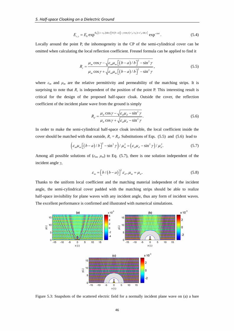
5. Half‐space Cloaking on a Dielectric Ground 

46 

( ) ( ) ( ){ }0 sin / cos ' / ' sin, 0 exp exp .P P P Pik x x b b a y r r x i t

c zE E γ γ γ ω− − − +⎡ ⎤ −⎣ ⎦= (5.4)

Locally around the point P, the inhomogeneity in the CP of the semi-cylindrical cover can be

omitted when calculating the local reflection coefficient. Fresnel formula can be applied to find it

( )

( )

2 2

2 2

cos / sin,

cos / sin

m m mc

m m m

b a bR

b a b

μ γ ε μ γ

μ γ ε μ γ

− − −⎡ ⎤⎣ ⎦=+ − −⎡ ⎤⎣ ⎦

(5.5)

where εm and μm are the relative permittivity and permeability of the matching strips. It is

surprising to note that Rc is independent of the position of the point P. This interesting result is

critical for the design of the proposed half-space cloak. Outside the cover, the reflection

coefficient of the incident plane wave from the ground is simply

2

2

cos sin.

cos sind d d

d

d d d

Rμ γ ε μ γ

μ γ ε μ γ

− −=

+ − (5.6)

In order to make the semi-cylindrical half-space cloak invisible, the local coefficient inside the

cover should be matched with that outside, Rc = Rd. Substitutions of Eqs. (5.5) and (5.6) lead to

( )( ) ( )2 2 2 2 2/ sin / sin / .m m m d d db a bε μ γ μ ε μ γ μ− − = −⎡ ⎤⎣ ⎦ (5.7)

Among all possible solutions of (εm, μm) to Eq. (5.7), there is one solution independent of the

incident angle γ,

( ) 2/ , .m d m db b aε ε μ μ= − =⎡ ⎤⎣ ⎦ (5.8)

Thanks to the uniform local coefficient and the matching material independent of the incident

angle, the semi-cylindrical cover padded with the matching strips should be able to realize

half-space invisibility for plane waves with any incident angle, thus any form of incident waves.

The excellent performance is confirmed and illustrated with numerical simulations.

Figure 5.3: Snapshots of the scattered electric field for a normally incident plane wave on (a) a bare

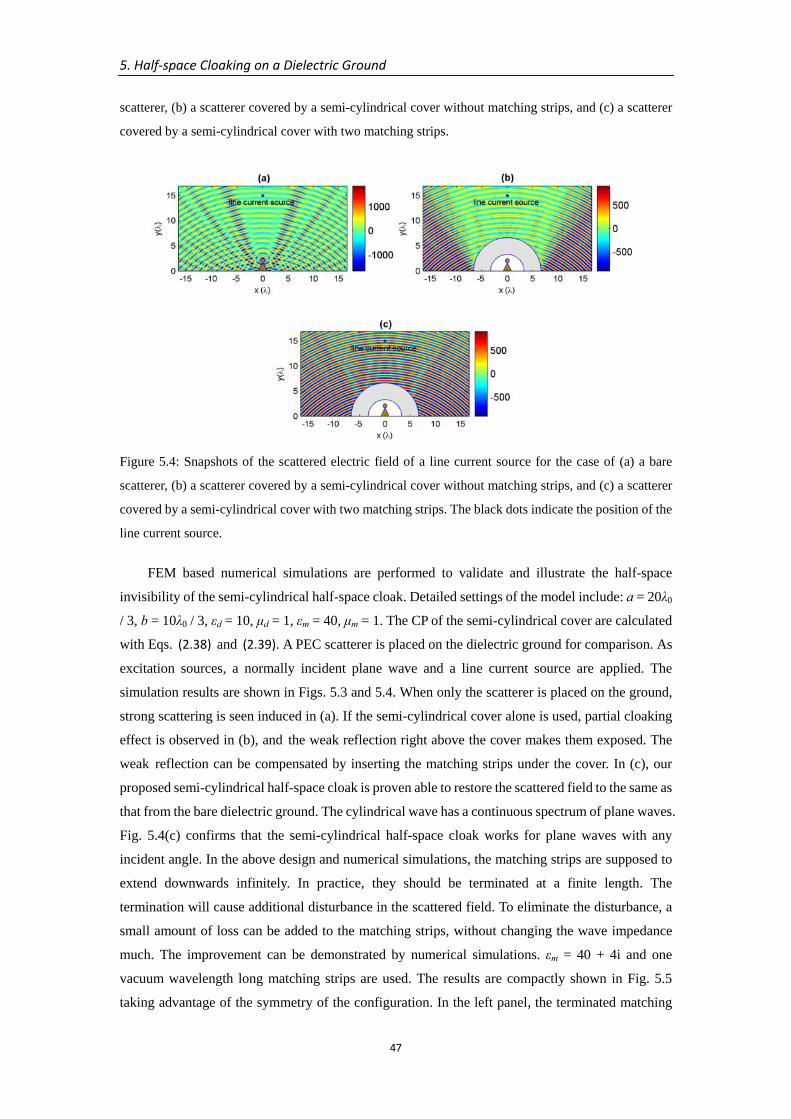
5. Half‐space Cloaking on a Dielectric Ground 

47 

scatterer, (b) a scatterer covered by a semi-cylindrical cover without matching strips, and (c) a scatterer

covered by a semi-cylindrical cover with two matching strips.

Figure 5.4: Snapshots of the scattered electric field of a line current source for the case of (a) a bare

scatterer, (b) a scatterer covered by a semi-cylindrical cover without matching strips, and (c) a scatterer

covered by a semi-cylindrical cover with two matching strips. The black dots indicate the position of the

line current source.

FEM based numerical simulations are performed to validate and illustrate the half-space

invisibility of the semi-cylindrical half-space cloak. Detailed settings of the model include: a = 20λ0

/ 3, b = 10λ0 / 3, εd = 10, μd = 1, εm = 40, μm = 1. The CP of the semi-cylindrical cover are calculated

with Eqs. (2.38) and (2.39). A PEC scatterer is placed on the dielectric ground for comparison. As

excitation sources, a normally incident plane wave and a line current source are applied. The

simulation results are shown in Figs. 5.3 and 5.4. When only the scatterer is placed on the ground,

strong scattering is seen induced in (a). If the semi-cylindrical cover alone is used, partial cloaking

effect is observed in (b), and the weak reflection right above the cover makes them exposed. The

weak reflection can be compensated by inserting the matching strips under the cover. In (c), our

proposed semi-cylindrical half-space cloak is proven able to restore the scattered field to the same as

that from the bare dielectric ground. The cylindrical wave has a continuous spectrum of plane waves.

Fig. 5.4(c) confirms that the semi-cylindrical half-space cloak works for plane waves with any

incident angle. In the above design and numerical simulations, the matching strips are supposed to

extend downwards infinitely. In practice, they should be terminated at a finite length. The

termination will cause additional disturbance in the scattered field. To eliminate the disturbance, a

small amount of loss can be added to the matching strips, without changing the wave impedance

much. The improvement can be demonstrated by numerical simulations. εm = 40 + 4i and one

vacuum wavelength long matching strips are used. The results are compactly shown in Fig. 5.5

taking advantage of the symmetry of the configuration. In the left panel, the terminated matching

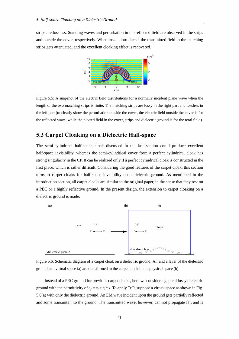
5. Half‐space Cloaking on a Dielectric Ground 

48 

strips are lossless. Standing waves and perturbation in the reflected field are observed in the strips

and outside the cover, respectively. When loss is introduced, the transmitted field in the matching

strips gets attenuated, and the excellent cloaking effect is recovered.

Figure 5.5: A snapshot of the electric field distributions for a normally incident plane wave when the

length of the two matching strips is finite. The matching strips are lossy in the right part and lossless in

the left part (to clearly show the perturbation outside the cover, the electric field outside the cover is for

the reflected wave, while the plotted field in the cover, strips and dielectric ground is for the total field).

5.3 Carpet Cloaking on a Dielectric Half-space

The semi-cylindrical half-space cloak discussed in the last section could produce excellent

half-space invisibility, whereas the semi-cylindrical cover from a perfect cylindrical cloak has

strong singularity in the CP. It can be realized only if a perfect cylindrical cloak is constructed in the

first place, which is rather difficult. Considering the good features of the carpet cloak, this section

turns to carpet cloaks for half-space invisibility on a dielectric ground. As mentioned in the

introduction section, all carpet cloaks are similar to the original paper, in the sense that they rest on

a PEC or a highly reflective ground. In the present design, the extension to carpet cloaking on a

dielectric ground is made.

Figure 5.6: Schematic diagram of a carpet cloak on a dielectric ground: Air and a layer of the dielectric

ground in a virtual space (a) are transformed to the carpet cloak in the physical space (b).

Instead of a PEC ground for previous carpet cloaks, here we consider a general lossy dielectric

ground with the permittivity of εg = εr + εi * i. To apply TrO, suppose a virtual space as shown in Fig.

5.6(a) with only the dielectric ground. An EM wave incident upon the ground gets partially reflected

and some transmits into the ground. The transmitted wave, however, can not propagate far, and is

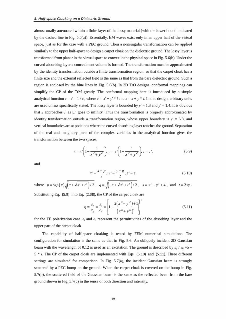
5. Half‐space Cloaking on a Dielectric Ground 

49 

almost totally attenuated within a finite layer of the lossy material (with the lower bound indicated

by the dashed line in Fig. 5.6(a)). Essentially, EM waves exist only in an upper half of the virtual

space, just as for the case with a PEC ground. Then a nonsingular transformation can be applied

similarly to the upper half-space to design a carpet cloak on the dielectric ground. The lossy layer is

transformed from planar in the virtual space to convex in the physical space in Fig. 5.6(b). Under the

curved absorbing layer a concealment volume is formed. The transformation must be approximated

by the identity transformation outside a finite transformation region, so that the carpet cloak has a

finite size and the external reflected field is the same as that from the bare dielectric ground. Such a

region is enclosed by the blue lines in Fig. 5.6(b). In 2D TrO designs, conformal mappings can

simplify the CP of the TrM greatly. The conformal mapping here is introduced by a simple

analytical function z = z' – 1 / z', where z' = x' + y' * i and z = x + y * i. In this design, arbitrary units

are used unless specifically stated. The lossy layer is bounded by y' = 1.3 and y' = 1.4. It is obvious

that z approaches z' as |z'| goes to infinity. Thus the transformation is properly approximated by

identity transformation outside a transformation region, whose upper boundary is y' = 5.8, and

vertical boundaries are at positions where the curved absorbing layer touches the ground. Separation

of the real and imaginary parts of the complex variables in the analytical function gives the

transformation between the two spaces,

2 2 2 2

1 1' 1 , ' 1 , ',' ' ' '

x x y y z zx y x y

⎛ ⎞ ⎛ ⎞= − = + =⎜ ⎟ ⎜ ⎟+ +⎝ ⎠ ⎝ ⎠

(5.9)

and

' , ' , ' ,2 2

x p y qx y z z+ += = = (5.10)

where ( ) ( )2 2sgn / 2p x s s t= + + , ( )2 2 / 2q s s t= − + + , 2 2 4s x y= − + , and 2t xy= .

Substituting Eq. (5.9) into Eq. (2.38), the CP of the carpet cloak are

( )( )

12 2

22 20

2 ' ' 11

' 'l c

g

x y

x y

ε εη

ε ε

−⎡ ⎤− +⎢ ⎥≡ = = +⎢ ⎥+⎣ ⎦

(5.11)

for the TE polarization case. εl and εc represent the permittivities of the absorbing layer and the

upper part of the carpet cloak.

The capability of half-space cloaking is tested by FEM numerical simulations. The

configuration for simulation is the same as that in Fig. 5.6. An obliquely incident 2D Gaussian

beam with the wavelength of 0.12 is used as an excitation. The ground is described by εg / ε0 =5 –

5 * i. The CP of the carpet cloak are implemented with Eqs. (5.10) and (5.11). Three different

settings are simulated for comparison. In Fig. 5.7(a), the incident Gaussian beam is strongly

scattered by a PEC bump on the ground. When the carpet cloak is covered on the bump in Fig.

5.7(b), the scattered field of the Gaussian beam is the same as the reflected beam from the bare

ground shown in Fig. 5.7(c) in the sense of both direction and intensity.

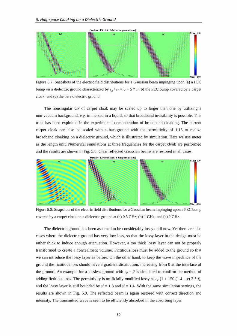
5. Half‐space Cloaking on a Dielectric Ground 

50 

Figure 5.7: Snapshots of the electric field distributions for a Gaussian beam impinging upon (a) a PEC

bump on a dielectric ground characterized by εg / ε0 = 5 + 5 * i, (b) the PEC bump covered by a carpet

cloak, and (c) the bare dielectric ground.

The nonsingular CP of carpet cloak may be scaled up to larger than one by utilizing a

non-vacuum background, e.g. immersed in a liquid, so that broadband invisibility is possible. This

trick has been exploited in the experimental demonstration of broadband cloaking. The current

carpet cloak can also be scaled with a background with the permittivity of 1.15 to realize

broadband cloaking on a dielectric ground, which is illustrated by simulation. Here we use meter

as the length unit. Numerical simulations at three frequencies for the carpet cloak are performed

and the results are shown in Fig. 5.8. Clear reflected Gaussian beams are restored in all cases.

Figure 5.8: Snapshots of the electric field distributions for a Gaussian beam impinging upon a PEC bump

covered by a carpet cloak on a dielectric ground at (a) 0.5 GHz; (b) 1 GHz; and (c) 2 GHz.

The dielectric ground has been assumed to be considerably lossy until now. Yet there are also

cases where the dielectric ground has very low loss, so that the lossy layer in the design must be

rather thick to induce enough attenuation. However, a too thick lossy layer can not be properly

transformed to create a concealment volume. Fictitious loss must be added to the ground so that

we can introduce the lossy layer as before. On the other hand, to keep the wave impedance of the

ground the fictitious loss should have a gradient distribution, increasing from 0 at the interface of

the ground. An example for a lossless ground with εg = 2 is simulated to confirm the method of

adding fictitious loss. The permittivity is artificially modified lossy as εg [1 + 150 (1.4 – y) 2 * i],

and the lossy layer is still bounded by y' = 1.3 and y' = 1.4. With the same simulation settings, the

results are shown in Fig. 5.9. The reflected beam is again restored with correct direction and

intensity. The transmitted wave is seen to be efficiently absorbed in the absorbing layer.

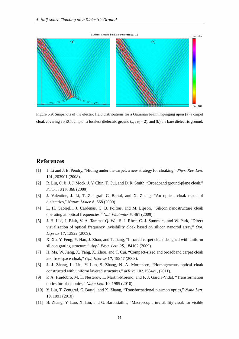
5. Half‐space Cloaking on a Dielectric Ground 

51 

Figure 5.9: Snapshots of the electric field distributions for a Gaussian beam impinging upon (a) a carpet

cloak covering a PEC bump on a lossless dielectric ground (εg / ε0 = 2), and (b) the bare dielectric ground.

References [1] J. Li and J. B. Pendry, “Hiding under the carpet: a new strategy for cloaking,” Phys. Rev. Lett.

101, 203901 (2008). [2] R. Liu, C. Ji, J. J. Mock, J. Y. Chin, T. Cui, and D. R. Smith, “Broadband ground-plane cloak,”

Science 323, 366 (2009). [3] J. Valentine, J. Li, T. Zentgraf, G. Bartal, and X. Zhang, “An optical cloak made of

dielectrics,” Nature Mater. 8, 568 (2009). [4] L. H. Gabrielli, J. Cardenas, C. B. Poitras, and M. Lipson, “Silicon nanostructure cloak

operating at optical frequencies,” Nat. Photonics 3, 461 (2009). [5] J. H. Lee, J. Blair, V. A. Tamma, Q. Wu, S. J. Rhee, C. J. Summers, and W. Park, “Direct

visualization of optical frequency invisibility cloak based on silicon nanorod array,” Opt. Express 17, 12922 (2009).

[6] X. Xu, Y. Feng, Y. Hao, J. Zhao, and T. Jiang, “Infrared carpet cloak designed with uniform silicon grating structure,” Appl. Phys. Lett. 95, 184102 (2009).

[7] H. Ma, W. Jiang, X. Yang, X. Zhou, and T. Cui, “Compact-sized and broadband carpet cloak and free-space cloak,” Opt. Express 17, 19947 (2009).

[8] J. J. Zhang, L. Liu, Y. Luo, S. Zhang, N. A. Mortensen, “Homogeneous optical cloak constructed with uniform layered structures,” arXiv:1102.1584v1, (2011).

[9] P. A. Huidobro, M. L. Nesterov, L. Martín-Moreno, and F. J. García-Vidal, “Transformation optics for plasmonics,” Nano Lett. 10, 1985 (2010).

[10] Y. Liu, T. Zentgraf, G. Bartal, and X. Zhang, “Transformational plasmon optics,” Nano Lett. 10, 1991 (2010).

[11] B. Zhang, Y. Luo, X. Liu, and G. Barbastathis, “Macroscopic invisibility cloak for visible

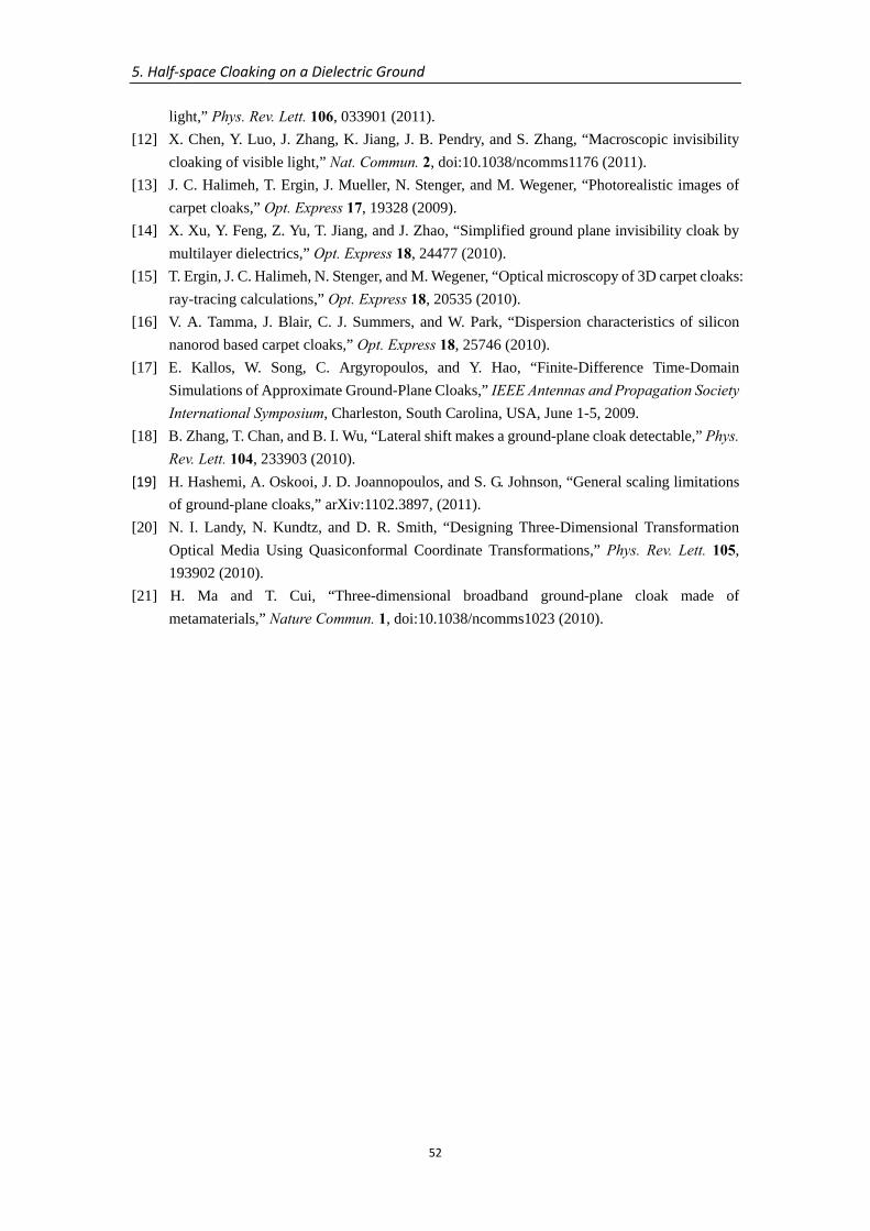
5. Half‐space Cloaking on a Dielectric Ground 

52 

light,” Phys. Rev. Lett. 106, 033901 (2011). [12] X. Chen, Y. Luo, J. Zhang, K. Jiang, J. B. Pendry, and S. Zhang, “Macroscopic invisibility

cloaking of visible light,” Nat. Commun. 2, doi:10.1038/ncomms1176 (2011). [13] J. C. Halimeh, T. Ergin, J. Mueller, N. Stenger, and M. Wegener, “Photorealistic images of

carpet cloaks,” Opt. Express 17, 19328 (2009). [14] X. Xu, Y. Feng, Z. Yu, T. Jiang, and J. Zhao, “Simplified ground plane invisibility cloak by

multilayer dielectrics,” Opt. Express 18, 24477 (2010). [15] T. Ergin, J. C. Halimeh, N. Stenger, and M. Wegener, “Optical microscopy of 3D carpet cloaks:

ray-tracing calculations,” Opt. Express 18, 20535 (2010). [16] V. A. Tamma, J. Blair, C. J. Summers, and W. Park, “Dispersion characteristics of silicon

nanorod based carpet cloaks,” Opt. Express 18, 25746 (2010). [17] E. Kallos, W. Song, C. Argyropoulos, and Y. Hao, “Finite-Difference Time-Domain

Simulations of Approximate Ground-Plane Cloaks,” IEEE Antennas and Propagation Society International Symposium, Charleston, South Carolina, USA, June 1-5, 2009.

[18] B. Zhang, T. Chan, and B. I. Wu, “Lateral shift makes a ground-plane cloak detectable,” Phys. Rev. Lett. 104, 233903 (2010).

[19] H. Hashemi, A. Oskooi, J. D. Joannopoulos, and S. G. Johnson, “General scaling limitations of ground-plane cloaks,” arXiv:1102.3897, (2011).  

[20] N. I. Landy, N. Kundtz, and D. R. Smith, “Designing Three-Dimensional Transformation Optical Media Using Quasiconformal Coordinate Transformations,” Phys. Rev. Lett. 105, 193902 (2010).

[21] H. Ma and T. Cui, “Three-dimensional broadband ground-plane cloak made of metamaterials,” Nature Commun. 1, doi:10.1038/ncomms1023 (2010).

 

53 

6. Conclusion and Future Work

In this thesis, we have focused on the theory of TrO and its usage for invisibility cloak designs.

The theory of TrO is elaborated and extended. The concept of inverse TrO is established and used

to analyze reflection from FECT media. A novel design method of reduced 2D cloaks of arbitrary

shapes is introduced and validated. We propose two new designs for cloaking objects on a

dielectric ground as well.

Based on the CP of a perfect 3D cloak with mirror symmetry on the symmetry plane, we

introduce an intuitive and effective method to construct a reduced 2D cloak of arbitrary shape.

Two examples, an elliptic and a bow-tie shaped reduced cloak, are designed and numerically

simulated to validate and illustrate the effectiveness of the method.

As a complementary concept to TrO, we consider a general idea of inverse TrO. 2D inverse

TrO is specifically developed to study reflection at the boundary of an FECT medium within the

framework of TrO. Different from the FECT, a whole space mapping between the physical space

and a virtual space is realized by an inverse transformation which is continuous across the

boundary. Necessary and sufficient condition of reflectionlessness is derived as a special result.

For the convenience of some particular applications, we have investigated half-space

cloaking on dielectric grounds. For the first time, we propose a semi-cylindrical half-space cloak

to achieve invisibility on a dielectric ground. Two carefully designed matching strips are inserted

underneath half of a perfect cylindrical cloak to induce proper reflection. The local reflection

coefficient is calculated analytically and matched to that from the bare ground. Thus the half-space

cloak can give rather good half-space invisibility.

The carpet cloak is an important idea for the accomplishment of half-space cloaking. We

extend the original design of the carpet cloak on a PEC ground to a dielectric ground. Taking

advantage of a lossy layer in a virtual space, a carpet cloak with an additional absorbing layer is

obtained to cloak objects on a dielectric ground. Through numerical simulations, both direction

and intensity of reflected Gaussian beams are restored to the same state as in the case of the bare

dielectric ground.

As for the matter of future work, we can say that there are several ongoing hot topics in the

field of TrO and invisibility cloaks. Currently, the realization of invisibility cloaks for practical

usage has been extensively studied. For example, 3D full-space invisibility cloaks, carpet cloaks

and geometrical optical cloaks have all been investigated in recent research. Quasi-conformal

mapping has also been proposed for 3D device designs with isotropic media. The theory of TrO is

currently generalized further to include more diverse EM media in the framework.

6. Conclusion and Future Work 

54 

 

55 

7. Summary of Contributions

Paper A. Cloaking an object on a dielectric half-space

Pu Zhang, Yi Jin, and Sailing He, “Cloaking an object on a dielectric half-space,” Opt. Express, 16, 3161 (2008).

Contribution of the author: Design and analysis of the half-space cloak. Numerical simulation of the proposed device. The first draft of the manuscript.

Paper B. Obtaining a nonsingular two-dimensional cloak of complex shape from a perfect three-dimensional cloak

Pu Zhang, Yi Jin, and Sailing He, “Obtaining a nonsingular two-dimensional cloak of complex shape from a perfect three-dimensional cloak,” Appl. Phys. Lett., 93, 243502 (2008).

Contribution of the author: Introduction of the design method. Calculations of material parameters for two examples. Numerical simulation of the reduced cloaks. The first draft of the manuscript.

Paper C. Inverse Transformation Optics and Reflection Analysis for Two-Dimensional Finite-Embedded Coordinate Transformation

Pu Zhang, Yi Jin, and Sailing He, “Inverse Transformation Optics and Reflection Analysis for Two-Dimensional Finite-Embedded Coordinate Transformation,” IEEE J. Sel. Top. Quant. Electron., 16, 427 (2010).

Contribution of the author: Proposal of the concept of inverse TrO. Calculation of the reflection from FECT media and reflectionless condition. Numerical simulation of examples, and the first draft of the manuscript.

Paper D. Carpet cloaking on a dielectric half-space

Pu Zhang, Michaël Lobet, and Sailing He, “Carpet cloaking on a dielectric half-space,” Opt. Express, 18, 18158 (2010).

Contribution of the author: Propose the design of carpet cloak on a dielectric ground. Analytical and numerical analysis of the proposed device, and the first draft of the manuscript.