Theory and Design of Statically Balanced Tensegrity Mechanisms · Tensegrity structures, or tensegrities, are a special type of prestressed pin-jointed bar frameworks with unique

Theory and Design of

Statically Balanced Tensegrity Mechanisms

Department of BioMechanical Engineering

Faculty of Mechanical, Maritime and Materials Engineering

MSc. Thesis

Mark SchenkFebruary 2006

Report title: Theory and Design of Statically Balanced Tensegrity MechanismsReport type: MSc. ThesisReport number: 993

Author: Mark SchenkDate: February 2006

Institute: Delft University of TechnologyFaculty of Mechanical, Maritime and Materials EngineeringDepartment of BioMechancial Engineering

Exam committee: prof. dr. ir. P.A. Wieringadr. ir. J.L. Herderdr. S.D. Guestdr. ir. A.L. Schwab

i

ii

Preface

This Master’s Thesis concludes my research on Statically Balanced TensegrityMechanisms, at the Delft University of Technology. The concept of tenseg-rity structures had caught my imagination from the outset, and the combina-tion with static balancing added another exciting dimension. The research waslargely theoretical, but – initially to my own surprise – I thoroughly enjoyedthe process of trying to understand the intricacies of the stiffness of prestressedstructures. I believe my efforts paid off, and the result lies before you.

During my project I had help from a lot of people, in manners great and small.All who helped me will know they have, and I’m grateful to them. Still, I havea few words of particular thanks.

First of all to my supervisor Just Herder, who is possibly even more enthusiasticabout the topic than I am. Thanks for all the time you devoted to, and interestyou showed in, my research!

An important part of the theory was developed during my four month internshipat the Cambridge University Engineering Department, and I’m very grateful toSimon Guest for hosting me, as well as for all the valuable help and discussionsafter my stay.

I would further like to thank Professor Connelly for some very fruitful discussionsduring my brief visit to Cambridge in October.

To the various students also working in the graduation workspace at MMS:thanks for the fun working environment! The seemingly endless supply ofSenseo coffee, discussions on the benefits of using LATEX, exclamations on thedownsides of using LATEX, problems with Matlab, weekend stories, drinkingstories, anything-but-work stories; it all combined to make this a very pleas-ant setting to finish my last months as a student. Special thanks is due toDaan ‘Don V’ Venekamp, who always patiently listened to my rambles, proof-read my paper, and now knows more about tensegrities than he ever would haveliked!

Last but not least: I would not have been able to study and do this research inthe first place, if it hadn’t been for the continuous support of my parents. Dankjullie wel!


iii

iv

Summary

The fields of static balancing and tensegrity structures are combined into stati-cally balanced tensegrity mechanisms. This combination results in a new class ofprestressed structures that behave like mechanisms: although member lengthsand orientations change, they can be deformed into a wide range of positions,while continuously remaining in equilibrium; in other words, the structures havezero stiffness. The key to these structures is the use of zero-free-length springsas tension members.

The tools of structural engineering were used to search for, and understand,zero-stiffness modes in the tangent stiffness matrix of prestressed pin-jointedbar frameworks. To this end the recently uncovered parallels between struc-tural engineering and mathematical rigidity theory were exploited. Mathemati-cal literature described that affine transformations preserve the equilibrium of atensegrity structure; these findings gained value when translated from a mathe-matical concept into the engineering terms rigid-body motions, shear and dila-tion. Not only did these transformations prove to be instrumental for describingzero stiffness, but it also provided new insight in the form-finding methods fortensegrity structures: the minimum nullity requirement for the stress matrix isformed by the affine transformations.

In this research it was shown that affine transformations of the structure thatpreserve the length of conventional members are zero-stiffness modes valid overfinite displacements: these are statically balanced zero-stiffness modes. What ismore, for prestress stable structures with a positive semi-definite stress matrix ofmaximal rank – meaning there are only affine transformations in its nullspace –those are the only possible zero-stiffness modes. The length-preserving affinetransformations exist if and only if the directions of the conventional memberslie on a conic at infinity. If all conventional member directions lie on a conic,the number of independent length-preserving affine transformations can then befound with a simple counting rule.

A systematic analysis of the zero-stiffness modes in the tangent stiffness matrixof a prestressed pin-jointed bar framework yielded several interesting scenariosthat warrant further attention, as they cannot be fully described within thecurrently developed framework.

Finally, a demonstration prototype was designed and constructed to illustratethe properties of statically balanced tensegrity mechanisms; the prototype servesas a proof of concept, not as a practically applicable design. Prior to construc-tion, the range of motion of the tensegrity used for the prototype was extensivelyanalysed using the analytic equilibrium conditions. The results were instrumen-tal in dimensioning the prototype.

v

vi

Contents

Preface iii

Summary v

1 Introduction 1

1.1 Outline . . . . . . . . . . . . . . . . . . . . . . . . . . . . . . . . 2

2 Zero Stiffness Tensegrity Structures 3

2.1 Introduction . . . . . . . . . . . . . . . . . . . . . . . . . . . . . . 3

2.2 Equilibrium and stiffness of prestressed structures . . . . . . . . 5

2.3 Affine transformations and zero-stiffness modes . . . . . . . . . . 8

2.4 Length-preserving affine transformations . . . . . . . . . . . . . . 12

2.5 Example . . . . . . . . . . . . . . . . . . . . . . . . . . . . . . . . 15

2.6 Summary and Conclusions . . . . . . . . . . . . . . . . . . . . . . 18

3 Overview of Zero Stiffness in Prestressed Bar Frameworks 21

3.1 Introduction . . . . . . . . . . . . . . . . . . . . . . . . . . . . . . 21

3.2 Stiffness of prestressed structures . . . . . . . . . . . . . . . . . . 22

3.3 Zero stiffness and matrix nullspace . . . . . . . . . . . . . . . . . 25

3.4 Contributions of K and Ω cancel out . . . . . . . . . . . . . . . . 29

3.5 Conclusion . . . . . . . . . . . . . . . . . . . . . . . . . . . . . . 30

4 Conclusions 33

Bibliography 35

Appendices

A Tensegrity Equilibrium 37

A.1 Introduction . . . . . . . . . . . . . . . . . . . . . . . . . . . . . . 37

A.2 Equilibrium configuration . . . . . . . . . . . . . . . . . . . . . . 37

A.3 Twist angle . . . . . . . . . . . . . . . . . . . . . . . . . . . . . . 39

A.4 Equilibrium tensions . . . . . . . . . . . . . . . . . . . . . . . . . 40

A.5 Literature comparison . . . . . . . . . . . . . . . . . . . . . . . . 42

A.6 Spring stiffness ratios . . . . . . . . . . . . . . . . . . . . . . . . . 44

A.7 Conclusion . . . . . . . . . . . . . . . . . . . . . . . . . . . . . . 45

vii

CONTENTS

B Tangent Stiffness Matrix 47

B.1 Introduction . . . . . . . . . . . . . . . . . . . . . . . . . . . . . . 47B.2 Modified axial stiffness . . . . . . . . . . . . . . . . . . . . . . . . 47B.3 Geometrically non-linear FEA . . . . . . . . . . . . . . . . . . . . 50B.4 Comparison . . . . . . . . . . . . . . . . . . . . . . . . . . . . . . 52B.5 Conclusion . . . . . . . . . . . . . . . . . . . . . . . . . . . . . . 53

C MATLAB Code Description 55

C.1 Introduction . . . . . . . . . . . . . . . . . . . . . . . . . . . . . . 55C.2 Code outline . . . . . . . . . . . . . . . . . . . . . . . . . . . . . 55C.3 Custom functions . . . . . . . . . . . . . . . . . . . . . . . . . . . 56C.4 Various remarks . . . . . . . . . . . . . . . . . . . . . . . . . . . 57C.5 Conclusion . . . . . . . . . . . . . . . . . . . . . . . . . . . . . . 57

D Prototype Design 59

D.1 Introduction . . . . . . . . . . . . . . . . . . . . . . . . . . . . . . 59D.2 Design requirements . . . . . . . . . . . . . . . . . . . . . . . . . 59D.3 Prototype description . . . . . . . . . . . . . . . . . . . . . . . . 60D.4 Design detailing . . . . . . . . . . . . . . . . . . . . . . . . . . . . 62D.5 Design Evaluation . . . . . . . . . . . . . . . . . . . . . . . . . . 69

E Zero Stiffness Examples 79

E.1 Introduction . . . . . . . . . . . . . . . . . . . . . . . . . . . . . . 79E.2 ‘Babytoy’ equilibrium . . . . . . . . . . . . . . . . . . . . . . . . 79

F Future Work 85

F.1 Introduction . . . . . . . . . . . . . . . . . . . . . . . . . . . . . . 85F.2 Future work . . . . . . . . . . . . . . . . . . . . . . . . . . . . . . 85F.3 Conclusion . . . . . . . . . . . . . . . . . . . . . . . . . . . . . . 88

Bibliography 89

viii

Chapter 1

Introduction

This thesis concludes the efforts to investigate the theory and design of staticallybalanced tensegrity mechanisms, a hitherto unexplorered combination of twofields of research, tensegrity structures and statically balanced systems.

Tensegrity structures, or tensegrities, are a special type of prestressed pin-jointed bar frameworks with unique properties: the tension elements are usuallyreplaced by cables, resulting in aesthetic, light-weight structures that seem todefy gravity. The structures are generally both statically and kinematically in-determinate, and they derive their stability from the state of self-stress, whichstabilizes any internal mechanisms present.

Statically balanced systems are in equilibrium in every configuration in theirworkspace, even when no friction is present: they are neutrally stable, and havezero stiffness. As a consequence, these systems can be operated with muchless effort as compared to the unbalanced situation. Hence, static balancingis used for energy-efficient design in for instance prosthetics and rehabilitationtechnology. A classic every day example is the ‘Anglepoise’ desk lamp whichcan be positioned virtually anywhere without external force.

The combination of the two fields was expected to produce mechanical frame-works with very interesting properties: tensegrities that can be deformed into awide range of shapes without external work, and thus displaying mechanism-likeproperties. These structures are in a fascinating state of balance: during defor-mation, the internal forces remain in harmony, but they change and shift frommember to member. Understanding these structures was expected to providenew insights into both fields, and perhaps yield a more fundamental understand-ing of static balancing.

A note is due about the terminology of these structures, as they are at onceboth structure and mechanism. In the current research we have used the toolsof structural eningeering to analyse their properties, and will therefore refer tothem as zero stiffness tensegrity structures in the report. However, any practicalapplication would be for their mechanism properties, and hence the term stati-cally balanced tensegrity mechanisms would be more appropriate. In describingthese structures both terms are equally valid and may be used interchangeably.

1

Chapter 1

1.1 Outline

The results of the MSc. Thesis are presented as two papers, complementedwith a range of Appendices for background information. The papers appearas chapters in this report, but are written as free standing entities: each hasits own abstract, introduction and conclusions. This accounts for the fact thatsome sections appear to be duplicated in both papers.

The first paper describes the underlying theory of “Zero Stiffness TensegrityStructures” and contains the main novelties of the research. It recapitulates thestiffness analysis of tensegrity structures, and describes under which circum-stances the structure has zero stiffness when zero-free-length springs are added.The results are illustrated by the numerical analysis of a classic tensegrity.

The second paper complements the first and aims to fill up some of the gaps, byproviding a systematic “Overview of Zero Stiffness in Prestressed Bar Frame-works”, and as far as current knowledge allows, describing its nature. Someintriguing border cases are given, to illustrate the interesting work left.

The conclusion wraps up both papers and the current state of research, andsuggests viable directions for continuing the research.

Appendices The appendices provide (detailed) background information tothe work described in the papers. The equilibrium conditions and configurationsof a special class of prismic rotationally symmetric tensegrities are described inAppendix A. These play a special role in the developed theory about zero-stiffness structures, as they form an entire family of statically balanced struc-tures. The derivation and comparison of the formulation of the tangent stiffnessmatrix used extensively throughout the research is provided in Appendix B. Ap-pendix D describes in detail the design process of the demonstration prototype,and contains useful information about the design problems encountered. Ap-pendix E shows several examples of zero stiffness tensegrity structures, followedby an extensive list of suggestions for future research work in Appendix F.

CDROM Enclosed with the report is a CDROM, which aside from a digitalcopy of this report includes the Matlab code described in Appendix C, as wellas pdf copies of a lot of the references.

WWW This report is also available online, along with presentations andMatlab code, at: http://www.markschenk.com/tensegrity/

2

Chapter 2

Zero Stiffness TensegrityStructures

M.Schenka, S.D.Guestb, J.L.Herdera

aMechanical, Maritime and Materials Engineering, Delft University ofTechnology, Mekelweg 2, 2628 CD Delft, The Netherlands

b Department of Engineering, University of Cambridge, Trumpington Street,Cambridge CB2 1PZ, United Kingdom

Abstract

Tension members with a zero rest length allow the construction of tensegritystructures that are in equilibrium over a continuous range of positions and thusexhibit mechanism-like properties: they are neutrally stable, or equivalentlyhave zero stiffness. Those zero-stiffness modes are not internal mechanisms, asthey involve first-order changes in member length, but are a direct result of theuse of the special tension members. These modes correspond to an affine trans-formation of the structure that preserves the length of conventional members,and are present if and only if the directional vectors of those members lie on aconic. This geometric interpretation provides an entire family of zero stiffnesstensegrity structures.

Keywords: zero stiffness, tensegrity structures, tensegrity mechanisms, staticbalancing, affine transformations

2.1 Introduction

This paper will describe and analyse a new and special class of ‘tensegrity’structures that straddle the border between mechanisms and structures: al-though member lengths and orientations change, the structures can be deformedover large displacements whilst continuously remaining in equilibrium. In otherwords, they remain neutrally stable, require no external work to deform, and

3

Chapter 2

(a) (b) (c)

Figure 2.1: Static balancing: the three structures shown are in equilibriumfor any position of the bar, as long as in (a) the masses (black circles) arecorrectly chosen, and in (b) and (c) the springs are zero-free-length springs withappropriately chosen stiffness.

hence have zero stiffness. Although zero stiffness is uncommon in the theoryof stability, several examples exist. Tarnai (2003) describes two systems thatdisplay zero stiffness, respectively related to bifurcation of equilibrium paths,and to snap-through type loss of stability of unloaded structures in a state ofself-stress. These structures require specific external loads or states of self-stressto exhibit zero stiffness. The key to the structures discussed in this paper, how-ever, is the use of tension members that, in their working range, appear to havea zero rest length – their tension is proportional to their length. Such membersare not merely a mathematical abstraction; it is for instance possible to wind aclose-coiled spring with initial tension that ensures, when the spring is extended,that the exerted force is proportional to the length.

The utility of zero-free-length springs was initially exploited in the design ofthe classic ‘Anglepoise’ lamp (French and Widden, 2000), but is more generallyapplied in the field of static balancing (Herder, 2001)(see Figure 2.1). Staticallybalanced systems are in equilibrium in every configuration in their workspace,and as they require little to no effort to operate, they are used for energy-efficient design in for instance robotics and medical settings. Herder (2001)discovered some basic examples of statically balanced tensegrities, which formedthe inspiration for the current research. Acquired knowledge in this research issuspected to lead to a more fundamental understanding of, and new synthesistools for, statically balanced systems.

‘Tensegrity’ is a term that is not consistently defined in literature, see Motro(1992) for a discussion. Here we take it to mean free-standing prestressed pin-jointed structures, which are in general both statically and kinematically inde-terminate. The state of self-stress ensures that each member carries a non-zero,purely tensile or compressive load, under absence of external loads and con-straints. Previously, the analysis of tensegrity structures, either by a structuralmechanics approach (e.g. Pellegrino and Calladine, 1986) or a mathematicalrigidity theory approach (e.g. Connelly and Whiteley, 1996), has only beenconcerned with whether or not a structure is stable. We shall only considerstructures that, were they constructed with conventional tension and compres-sion members, are prestress stable (i.e. have a positive-definite tangent stiffnessmatrix, modulo rigid-body motions). The novel feature of this paper is that wethen replace some or all of the tension members with zero-free-length springs,in search of zero-stiffness modes.

4

Zero Stiffness Tensegrity Structures

The zero-stiffness tensegrities described in this paper walk a fine line betweenstructures and mechanisms. Here we shall refer to them as tensegrity structures,as we will be using the tools of structural engineering and not mechanism theory.For other purposes, the term tensegrity mechanisms might be more applicable.Practical applications of this new class of structure will most likely also takeplace on the borderline of structures and mechanisms, such as, for example,deployable structures which are in equilibrium throughout deployment.

There are clear hints to the direction taken in this paper in the affine transfor-mations considered by Connelly and Terrell (1995) or the ‘tensegrity similaritytransformation’ considered by Masic et al. (2005). Unlike in those papers, herethe affine transformations are translated from a mathematical abstraction intoa real physical response of structures that can be constructed.

The paper is laid out as follows. Section 2.2 recapitulates the equilibrium andstiffness analysis of prestressed structures. In particular it describes the con-sequences of using zero-free-length springs by means of a recent formulation ofthe tangent stiffness matrix. Section 2.3 introduces affine transformations andshows that affine modes which preserve the length of the conventional membersare statically balanced zero-stiffness modes. A general existence criterion forlength-preserving affine transformations is discussed in section 2.4. An exampleanalysis of a classic tensegrity structure fitted with zero-free-length springs, insection 2.5 illustrates the theory laid down priorly.

2.2 Equilibrium and stiffness of prestressed struc-tures

This section aims to lay the groundwork for the coming sections, by first brieflyrecapitulating the tensegrity form-finding method from rigidity theory, followedby the description of the tangent stiffness matrix that clearly shows the effectsof using zero-free-length springs. The section is concluded by a discussion ofzero-stiffness modes in conventional tensegrity structures.

2.2.1 Equilibrium position

This paper is primarily concerned with the stiffness of a tensegrity structure ina known configuration, and not with form finding, i.e. finding an initial equi-librium configuration (Tibert and Pellegrino, 2003). Nevertheless, a brief de-scription will be given, as there are interesting and useful parallels between thestiffness of a prestressed structure and the energy method of rigidity theory (or,equivalently, the engineering force density method) used in form finding.

The energy method in rigidity theory considers a stress state ω to be a stateof self-stress if the internal forces at every node sum to zero, i.e. the followingequilibrium condition holds at each node i

∑

j

ωij (pj − pi) = 0 (2.1)

5

Chapter 2

where pi are the coordinates for node i, and ωij is the tension in the memberconnecting nodes i and j, divided by the length of the member; ωij is referredto as a stress in rigidity theory, but is known in engineering as a force densityor tension coefficient. If all the nodal coordinates are written together as avector p, pT = [pT

1 ,pT2 , . . . ,pT

n ], the equilibrium equations at each node can becombined to obtain the matrix equation

Ωp = 0 (2.2)

where Ω is the stress matrix for the entire structure. In fact, because equa-tion 2.1 consists of the same coefficients for each of d dimensions, the stressmatrix can be written as the Kronecker product of a reduced stress matrix Ω

and a d-dimensional identity matrix Id

Ω = Ω ⊗ Id. (2.3)

The coefficients of the reduced stress matrix are then given, from equation 2.1,as

Ωij =

−ωij = −ωji if i 6= j, and i,j a member,∑

k 6=i ωik if i = j,

0 if there is no connection between i and j.(2.4)

Although the stress matrix is here defined entirely by equilibrium of the struc-ture, we shall see the same matrix recurring in the stiffness equations in sec-tion 2.2.2. This dual role of the stress matrix allows the combination and ap-plication of insights from rigidity theory – where the stress matrix has been theobject of study – to engineering stiffness analysis.

Form-finding methods require the symmetric matrix Ω to have a nullity N ≥d + 1, and thus for Ω a nullity N ≥ d(d + 1)1. If the nullity requirement is notmet, the only possible configurations of the structure will be in a subspace of alower dimension. For example, form finding in 3 dimensions would only be ableto produce planar equilibrium configurations (Tibert and Pellegrino, 2003). Thesignificance of this requirement will be further elucidated in section 2.3, whenaffine transformations are introduced. If Ω has a nullity equal to d(d + 1), weshall describe it as being of maximal rank.

2.2.2 Tangent stiffness matrix

Stability analysis considers small changes from an equilibrium position. For aprestressed structure account must be taken not only of the deformation of theelements and the consequent changes in internal tension, but also of the effects ofthe changing geometry on the orientation of already stressed elements. This re-sults in the tangent stiffness matrix Kt, that relates infinitesimal displacementsd to force perturbations f

Ktd = f . (2.5)

1The nullity of a square matrix is equal to its dimension minus its rank.

6


The tangent stiffness matrix is well-known in structural analysis, and manydifferent formulations for it exist (e.g. Murakami, 2001; Masic et al., 2005). Dif-ferent formulations with identical underlying assumptions will produce identi-cal numerical results, but may provide a different understanding of the stiffness.The formulation used in this paper is derived by Guest (2006), and incorporateslarge strains. It is written as

Kt = K + Ω

= AGAT + Ω (2.6)

where Ω is the stress matrix as described earlier, K is the modified materialstiffness matrix, A is the equilibrium matrix for the structure and G is a diag-onal matrix whose entries consist of the modified axial stiffness for each of themembers. The modified axial stiffness g is defined as

g = g − ω (2.7)

where g is the conventional axial stiffness and ω the tension coefficient. Forconventional members, g will be little different from g. It will certainly alwaysbe positive, and hence the matrix G will always be positive definite. However,for a zero-free-length spring, because the tension t is proportional to the length,t = gl, the tension coefficient is equal to the axial stiffness, ω = t/l = g, andthe modified axial stiffness g = g − ω = 0. Thus structures constructed withzero-free-length springs will have zeros along the diagonal of G correspondingto these members, and G will now only be positive semi-definite.

Normally, a zero axial stiffness would be equivalent to the removal of that mem-ber (Deng and Kwan, 2005). This is not the case for the zero modified axialstiffness of zero-free-length springs, because the contribution of the member isstill present in the stress matrix Ω. This leads to the observation that for zero-free-length springs the geometry (i.e. the equilibrium matrix A) is irrelevantand only the tension coefficient and member connectivity (i.e. the stress matrixΩ) define their reaction to displacements.

2.2.3 Zero-stiffness modes and internal mechanisms

The main interest of this paper lies in displacements that have a zero stiffness;in other words, displacements that are in the kernel, or nullspace, of the tangentstiffness matrix. A zero tangent stiffness for some deformation d requires, fromequation 2.6, either that Kd = −Ωd, or that both Kd and Ωd are zero. Wewill briefly discuss in section 2.3.3 why the first possibility is not of interest, andwill concentrate on the second case, i.e. d lies in the nullspace of both K andΩ.

For a conventional structure, as G is positive definite, the nullspace of K =AGAT is equal to the nullspace of AT , and hence AT d = 0. The matrixC = AT is the compatibility matrix (closely related to the rigidity matrix inrigidity theory) of the structure, and the extension of members e is given byCd = e; i.e. e = 0 for a zero-stiffness mode. Thus, for a conventional structure

7

Chapter 2

a zero tangent stiffness requires the deformation to be an internal mechanism:a deformation that to first order causes no member elongation. In addition Ωd

must be zero, which implies that the mechanism is not stabilized by the self-stress in the structure. One obvious mode is that rigid-body displacements ofthe entire structure will have no stiffness. However, in general there may alsobe other non-stiffened (higher-order) infinitesimal, or even finite, internal mech-anisms present (see e.g., Pellegrino and Calladine, 1986; Kangwai and Guest,1999). Infinitesimal mechanisms may eventually stiffen due to the higher-orderelongations of members, but finite internal mechanisms have no stiffness overa finite path. Thus, the stability of a structure requires that all displacementshave a positive stiffness. This means that, modulo rigid-body motions, all eigen-values of the tangent stiffness matrix are positive and the matrix is thus positivedefinite.

Some of the above observations change when a structure includes zero-free-length springs, which have modified axial stiffness g = 0. A key observation isthat the nullspace of K = AGAT is no longer the same as the nullspace of AT ,as G is now only positive semi-definite. The increased nullity of the modifiedmaterial stiffness matrix K is of great importance to this study, as it will proveto be key to finding the desired zero-stiffness modes (see section 2.3). Notethat the stress matrix Ω is invariant when zero-free-length springs are added tothe structure.

We introduce the term ‘statically balanced zero-stiffness mode’ to distinguishbetween zero-stiffness modes found in conventional tensegrity structures, suchas internal mechanisms and rigid-body motions, and (finite) zero-stiffness modesintroduced by the presence of zero-free-length springs. In contrast with (finite)internal mechanisms, these latter modes involve first-order changes in memberlength, and thus energy exchange among the members.

2.3 Affine transformations and zero-stiffness modes

This section introduces the concept of affine transformations, leading up to thekey conclusion that affine transformations that preserve the length of ‘conven-tional’ members are statically balanced zero-stiffness modes that are valid overfinite displacements. It shall further be argued that for prestress stable tenseg-rity structures with a positive semi-definite stress matrix of maximal rank, theseare the only possible zero-stiffness modes.

2.3.1 Affine transformations

As described in section 2.2.1, the equilibrium position of a freestanding tenseg-rity structure for a given state of self-stress is given by Ωp = 0. Under an affinetransformation of the nodal coordinates p this condition still holds (Connellyand Whiteley, 1996; Masic et al., 2005), and hence the new geometry is also inequilibrium for the same set of tension coefficients. An important consequencewhich had previously not explicitly been observed, is that affine transformationsof p hence remain in the nullspace of Ω.

8


(a)

(b)

(c) (d)

(e)

Figure 2.2: The independent affine transformations of an object (a) in 2D spaceare: (b) two translations, (c) one rotation, (d) one shear, (e) two dilations. Thetotal of 6 transformations complies with the d(d + 1) formula for d = 2.

Affine transformations are linear transformations of coordinates (of the wholeaffine plane onto itself) preserving collinearity. Thus, an affine transformationtransforms parallel lines into parallel lines and preserves ratios of distances alongparallel lines, as well as intermediacy (Coxeter, 1989, pp. 202). We write themas the transformation of the coordinates of node i

pi → Upi + w

where in d-dimensional space U is a d-by-d matrix, and w ∈ Ed. This providesa total of d(d + 1) independent affine transformations. Affine transformationsare well-known to engineers, but under a different guise. Recall that the squarematrix U can be expressed as the sum of a symmetric and a skew-symmetriccomponent. Then the half of the d(d + 1) affine transformations constituted byw and the skew-symmetric part of U, is better known to engineers as rigid-bodymotions (e.g. 6 rigid-body motions in 3-dimensional space). The interpretationof the other half – the symmetric part of U – is less obvious, but it turns out tobe equivalent to the basic strains found in continuum mechanics: shear and dila-tion. For instance, for a 3-dimensional strain, infinitesimal affine deformationsgive the six independent strain quantities (exx, eyy, ezz, exy, exz, eyz) (Love,1927). For two dimensions, the complete set of affine transformations is shownin Figure 2.2.

It is obvious that the equilibrium of a tensegrity structure holds for rigid-bodymotions, but it is less clear for the other affine transformations. This knowledgecan be used to great advantage in form finding to obtain new equilibrium shapes(Masic et al., 2005), but it also has important consequences for static balancingand the study of zero-stiffness modes. The above also clarifies the N ≥ d(d+1)nullity requirement for Ω found in form finding: there must be at least d(d + 1)affine transformations in the kernel of Ω if a solution for the form finding is tobe found in d-space – provided there are sufficient nodes to span d-space.

9

Chapter 2

2.3.2 Statically balanced zero-stiffness modes

A structure has a zero stiffness if for a given displacement vector d – in thenullspace of the tangent stiffness matrix Kt – the following equation

Ktd = Kd + Ωd

= AGAT d + Ωd = 0 (2.8)

returns zero. We focus here on the situation where both AGAT d and Ωd

are zero – other possibilities are discussed in section 2.3.3. We shall excludeinternal mechanisms by only considering tensegrity structures that when builtwith conventional elements would be stable for the given state of self-stress.Conventional elements are here understood to be tensile or compressive membersthat have a positive modified axial stiffness. Consequently, any zero-stiffnessmodes would be a result of the use of zero-free-length springs.

As shown in section 2.3.1, affine transformations of the coordinates p are in thenullspace of Ω. For a conventional structure, these modes (excluding the rigid-

body motions) are stabilized by the modified material stiffness matrix K. Forstructures with zero-free-length springs, however, the positive semi -definitenessof G and the resulting increased nullity in K will result in new zero-stiffnessmodes. The key therefore is in understanding the solutions to AGAT d = 0. Ifa displacement d is length-preserving for the conventional members, then

AT d = e (2.9)

returns zero-elongations for those conventional members. Now consider that

GAT d = Ge (2.10)

always returns zeros for the zero-free-length springs and non-zero for conven-tional members, due to the zero modified axial stiffness on the diagonal of G.Thus, a displacement d that preserves the length of conventional elements willsatisfy GAT d = 0 and will hence be in the nullspace of AGAT . Combiningthese observations, it is clear that for an affine transformation that preserves thelength of conventional members, both Kd and Ωd are zero and there is a stat-ically balanced zero-stiffness mode. This is illustrated by the simple staticallybalanced structure shown in Figure 2.3.

Note that when a member length remains constant, so does the tension and thusthe tension coefficient. This also follows from the fact that the stress matrix Ω

remains invariant under the affine transformation that results in new equilib-rium, and therefore, so do the tension coefficients. For zero-free-length springsthe tension coefficient is equal to their spring stiffness and will therefore alwaysbe constant, but for conventional members the only way a tension coefficientcan remain constant is when both length and tension are invariant.

Any modes in the tangent stiffness matrix are per definition infinitesimal dis-placements. This leads to the question whether the aforementioned staticallybalanced zero-stiffness modes merely hold for infinitesimal, or also for finitedeformations. The independence of the zero-free-length springs of their actual

10


Figure 2.3: Example of a 2D statically balanced structure consisting of twounconnected bars of differing lengths, and four zero-free-length springs of equalstiffness. When the bars are rotated with respect to each other, they remainin equilibrium and their movement thus has zero stiffness. In this example it isclear that the statically balanced mode is a combined shear and scale operationwhich preserves the bar lengths. Figure adapted from Herder (2001).

geometrical position for their contribution to Kt, suggests an affirmative an-swer to this question. Formalization of the fact that they are indeed finitezero-stiffness modes, takes a different approach, and will be deferred to section4.3 as it requires additional information.

2.3.3 Additional zero-stiffness modes

Using equation 2.6 for the tangent stiffness matrix, there are two distinct waysthe structure may have zero stiffness. Either the contributions of K and Ω

cancel out, or both are zero.

The situation where Kd = −Ωd is not fully understood, and no example struc-tures are known to the authors. For conventional structures it would also seem arather unlikely situation as for small strains the contributions of K are generallyan order of magnitude greater than those of Ω. Furthermore it would requirethe stress matrix Ω to have negative eigenvalues, which is undesirable as it maymake the structure unstable under certain loading conditions.

Throughout the previous sections we have focused on the case where the zero-stiffness mode is in the nullspace of both components of the tangent stiffnessmatrix. When zero-free-length springs are added to the structure, the nullspaceof the stress matrix is invariant, but the nullspace of K changes significantly.If the newly introduced nullvectors coincide with an affine transformation, thestructure has zero stiffness. However, the nullspace of Ω is in general not limitedto the affine transformations, and theoretically more combinations of the twonullspaces of K and Ω are possible. It is beyond the scope of this paper tosystematically analyse all possible combinations that produce a zero stiffness.

The situation is considerably simpler when considering structures with a pos-itive semi-definite stress matrix of maximal rank, which are prestress stablewhen constructed with solely conventional members. Under these conditionsthe length-preserving affine transformations are the only possible zero-stiffnessmodes. The maximal rank condition ensures that only affine transformationsare in the nullspace of the stress matrix, and by virtue of the prestress stabil-ity condition those are not internal mechanisms. The positive semi-definitenessrequirement ensures that there are no negative eigenvalues in the stress matrixthat can cause zero stiffness by the contributions of K and Ω cancelling each

11

Chapter 2

other out: Kd = −Ωd. These are not considered restrictive requirements asmany classic tensegrity structures already seem to comply.

The above conditions provide an additional benefit, as they ensure that anyinternal mechanisms remain stabilized by the state of self-stress throughout thedisplacement along the finite affine transformation. The number of internalmechanisms will always remain constant under an affine transformation, as therank of the equilibrium matrix is constant under a linear transformation (withthe exception of a projection on a lower dimension). Disregarding the latterscenario, in all other cases the maximal rank positive semi-definite stress matrix(which is invariant under the affine transformation) will ensure that the state ofself-stress will always impart a first-order stiffness to the internal mechanisms.

2.4 Length-preserving affine transformations

In the previous section it has been shown that an affine transformation preserv-ing the length of conventional members is a statically balanced zero-stiffnessmode. In this section we will show that such a transformation exists if and onlyif the directions of the conventional members lie on a conic. The conic form willalso prove to be useful in establishing the finiteness of the found zero-stiffnessmode.

2.4.1 Length preservation and conic form

In order to understand under which circumstances the length of a member in-creases, decreases or stays the same under an affine transformation, we shallinvestigate the squares of the lengths of the members under the affine transfor-mation given by pi → Upi +w, where U is a d-by-d matrix, w ∈ Ed, and pi,pj

are the nodal coordinates:

L2 − L20 = |(Upi + w) − (Upj + w)|2 − |pi − pj |2

= (pi − pj)T UT U(pi − pj) − (pi − pj)

T Id(pi − pj)

= (pi − pj)T [UT U − Id](pi − pj)

= vT Qv

where Id denotes the d-dimensional identity matrix, and v = (pi − pj) is themember direction. From this calculation it is clear that the symmetric matrixQ = UT U − Id and its associated quadratic form determine when memberlengths increase, decrease or stay the same.

We are interested in the situation where vT Qv = 0. For the case of d = 3,with directions vT = [vx vy vz] and components of the symmetric Q given asqkl = qlk, this would take the following form

v2xq11 + 2vxvyq12 + 2vxvzq13 + v2

yq22 + 2vyvzq23 + v2zq33 = 0. (2.11)

Equation 2.11 defines a quadratic curve, which (in nondegenerate cases) corre-sponds to the intersection of a plane with (one or two nappes of) a cone: a conic

12


section (Weisstein, 1999). We can now see that a set of directions defined by

C = v ∈ Ed |vT Qv = 0 (2.12)

forms a conic at infinity. This conic is clearly defined since scalar multiples ofa vector satisfy the same quadratic equation, including the reversal of directionby a negative scalar. Generally one would expect C to be the set of lines fromthe origin to the points of, for example, an ellipse in some plane not throughthe origin (see Figure 2.4).

Supposing D is a set of directions in d-space, then there is an affine trans-formation pi → Upi + w that is not a rigid-body motion and that preserveslengths in the directions in D if and only if the directions in D lie on a conicat infinity. Or conversely, when the directions of certain members (in our caseconventional elements) lie on a conic given by Q = UT U− Id, their length willremain constant under the affine transformation U.

Of interest here are structures where all the conventional member directions lieon a conic, as the corresponding affine transformations will have zero stiffness.This is for instance clear for the structures shown in Table 2.1, where all thebar directions lie on a conic and the other members are zero-free-length springs.This leads to the observation that all the rotationally symmetric tensegritystructures discussed by Hinrichs (1984) and by Connelly and Terrell (1995) canhave zero stiffness, when the cables are replaced by appropriate zero-free-lengthsprings.

2.4.2 Number of zero-stiffness modes

Using the conic form, the number of independent length-preserving affine trans-formations of the structure can easily be determined. It holds that five pointsin a plane – no three of which collinear – uniquely determine a conic. Thisfollows from the fact that a conic section is a quadratic curve; e.g. dividingequation 2.11 by q11 leaves 5 constants. If there are less points, the conic isnot uniquely defined and there exists more than one conic that satisfies thequadratic curve.

As shown previously, when all conventional member directions lie on a conicthere exists a length-preserving affine transformation which has zero stiffness.However, if there are less than five unique member directions (i.e. unique pointson the conic section) there exists more than one conic, and thus more than onelength-preserving affine transformation. The number of additional conics (andthus zero-stiffness modes) is found by subtracting the number of unique pointson the conic section from the five required for uniqueness.

The above can now be summarized in the following counting rule for determiningthe number of zero-stiffness modes. Provided that all conventional memberdirections vi lie on a conic, and with k unique points on the conic section, thenumber of zero-stiffness modes is given by

k ≥ 6 → 1 zero-stiffness modek < 6 → (6 − k) zero-stiffness modes

(2.13)

13

Chapter 2

v1

v2

v3

origin

Figure 2.4: A conic intersected by a plane generates a conic section, which is aquadratic curve such as an ellipse, parabola or hyperbola. The directions vi onthe conic project onto points on the conic section.

Table 2.1: Number of statically balanced zero-stiffness modes for severalrotationally symmetric tensegrity structures discussed by Hinrichs (1984). Allbar directions lie on a conic, and thus when using appropriate zero-free-lengthsprings the structures will have zero stiffness. The number of bar directionson the conic and the number of zero-stiffness modes fit the counting ruleestablished in section 2.4.2.

Bar directions on conic 5 4 3Zero-stiffness modes 1 2 3

14


Note that only the number of member directions is relevant, not the number ofmembers. In other words, parallel members share a common member direction,and project onto a single point on the conic section. Furthermore, it is asyet unclear how to deal with two-dimensional structures, or structures that areprojected onto a lower dimension and are reduced to a planar configuration.

2.4.3 Finiteness of zero-stiffness mode

The conic form is also valuable for showing the finiteness of the statically bal-anced zero-stiffness modes. If the conventional members lie on a conic, as byprevious discussion, there exists an affine transformation that has zero stiffness.If we follow that zero stiffness path for an infinitesimal step, then in the newgeometry, because the step is an affine transformation, there will exist a newconic on which the conventional members lie, and hence there will again be azero-stiffness mode. As a result, the statically balanced zero-stiffness mode willbe finite.

2.5 Example

This section describes the numerical analysis of the classic tensegrity structureshown in Figure 2.5. Both the nature and number of the calculated zero-stiffnessmodes fit the theory laid down in previous sections. This is further illustratedby the construction of a physical model.

2.5.1 Numerical analysis

It is expected that when the cables are replaced by zero-free-length springs, thestructure will have three zero-stiffness modes, and that these modes are affinetransformations preserving the length of the three bars. This follows from theobservation that the structure has three bar directions on a conic, and thus byequation 2.13 there are three independent zero-stiffness modes.

The tangent stiffness of the structure has been found using the formulation ofequation 2.6 for two different cases. Firstly, with the structure consisting ofconventional elements, and secondly, when made from conventional compressivebars, but using zero-free-length springs as tension members. The equilibriumconfiguration has been calculated with the analytical solution of Connelly andTerrell (1995), and the level of self-stress – and thus the stress matrix – is identi-cal for both cases. All conventional elements have a ‘stiffness’ of EA = 100N, thehorizontal springs 1N/m and the vertical springs

√3N/m. The internal tension

of the structure is uniquely prescribed by these spring stiffnesses. The resultsare presented as the stiffness of each of the eigenmodes (excluding rigid-bodymotions) in Tables 2.2(a) and 2.2(b).

For the conventional structure all eigenvalues of the tangent stiffness matrix arepositive, and the stress matrix is of maximal rank. The system has an internalmechanism, which is stabilized by the state of self-stress. This can be seen in

15

Chapter 2

12

11

109

8

7

65

4

32

1

6

54

3

2

1

Figure 2.5: Rotationally symmetric tensegrity structure. The structure has acircumscribing radius R = 1, height H = 2 and the two parallel equilateraltriangles (nodes 1–3 and nodes 4–6) are rotated π/6 with respect to eachother.

Table 2.2: Stiffness of each of the eigenmodes, excluding rigid-body motions, for(a) the conventional structure and (b) the structure with zero-free-length springs

as tension members. The total stiffness Kt is the sum of the contributions of K

and Ω.(a)

Kt K Ω

5.6304 0.0174 5.613027.8384 26.1960 1.642427.8384 26.1960 1.642483.2190 79.1954 4.023683.2190 79.1954 4.0236107.3763 103.0749 4.3014107.3763 103.0749 4.3014113.8525 113.5350 0.3175132.5068 130.4743 2.0325132.5068 130.4743 2.0325176.2051 170.2051 6.0000225.4577 225.3881 0.0696

(b)

Kt K Ω

0.0000 0.0000 0.00000.0000 0.0000 0.00000.0000 0.0000 0.00005.6703 0.0267 5.64365.6703 0.0267 5.64365.7899 0.0174 5.77246.0000 0.0000 6.00006.0000 0.0000 6.00006.0000 0.0000 6.000075.5997 75.3721 0.227675.7193 75.3629 0.356475.7193 75.3629 0.3564

16


xy

z

z

x

xy

(a) (b) (c)

Figure 2.6: Fully symmetric zero-stiffness mode, with (a) 3D view, (b) top viewand (c) side view. All displacement vectors are of equal magnitude, and withequal z-component. In this mode the rotation angle between bottom and toptriangle remains constant throughout the displacement.

the first line of Table 2.2(a), where the K component is almost zero (it is not

precisely zero because the eigenvectors of K and Kt are not precisely aligned).

When zero-free-length springs are placed in the structure, three new zero-stiffness modes appear in Kt – the first three rows of Table 2.2(b) – which arelinearly dependent on the affine transformations for shear and dilation. Thesemodes can be considered in a symmetry-adapted form (Kangwai and Guest,1999) as a totally symmetric mode, and a pair of modes that are symmetric andantisymmetric with respect to a dihedral rotation. The fully symmetric modeis shown in Figure 2.6. It is purely dependent on scaling transformations, andcorresponds to a mode where the structure is compressed in the x-y plane andexpands in the z-direction.

In conclusion, the numerical results confirm the theoretical predictions: thezero-stiffness modes correspond to affine transformations, the bar lengths remainconstant – Cd returned zero for the bars – and the number of introduced zero-stiffness modes fits the counting rule established in section 2.4.2.

2.5.2 Physical model

To illustrate that the zero stiffness tensegrity structure is not merely mathe-matical, a demonstration prototype was constructed. It does not make use ofactual zero-free-length springs, but of conventional springs that are attachedalongside the bars such that the properties of zero-free-length springs are em-ulated. As gravity forces were not taken into account in the calculations, ifperfectly constructed, the prototype would collapse under its own weight. Thefriction in the system prevents this from happening, however. As a result thestructure requires some external work to deform, but it will nevertheless remainin equilibrium over a wide range of positions (see Figure 2.7).

17

Chapter 2

Figure 2.7: The demonstration model deformed in accordance with the sym-metrical zero-stiffness mode. The three positions shown do not correspond tothe extremes of the working range, as further deformation is still possible.

2.6 Summary and Conclusions

This paper has investigated the zero-stiffness modes introduced to tensegritystructures by the presence of zero-free-length springs. It was shown that underabsence of external loads and constraints, affine transformations that preservethe length of conventional members are statically balanced zero-stiffness modes.Those modes involve changing spring lengths, but require no energy to move,even over large displacements. For prestress stable tensegrities with a positivesemi-definite stress matrix of maximal rank, we further showed that these arethe only possible zero-stiffness modes introduced by the zero-free-length springs.

A general existence criterion was derived, and it was shown that such length-preserving affine transformations are present if and only if the directions of theconventional elements lie on a conic. This geometric interpretation revealed anentire family of tensegrity structures that can exhibit zero stiffness. A simplecounting rule was also found, which provides the number of independent length-preserving affine transformations.

By only considering tensegrity structures, the theory in this paper has severalinherent restrictions. Future work will attempt to resolve these aspects, startingwith the inclusion of external loads and nodal constraints in the analysis of pin-jointed structures. The next phase would be to apply the acquired knowledgeto non-pin-jointed structures, in order to describe statically balanced structuressuch as the ‘Anglepoise’ lamp in a generic way.

Finally, the construction of the physical model has illustrated that this type ofstructure is not yet suited for practical applications. Once difficulties such asaccuracy of spring stiffness ratio, presence of friction and overall complexity ofdesign have been overcome, a totally new class of structures, or mechanisms,will be available to engineers.

18


Acknowledgements

The authors wish to thank Professor Connelly (Cornell University) for the in-sight and proof of the link between conic form and length-preserving affinetransformations described in section 2.4.

Bibliography

Connelly, R., Terrell, M., 1995. Globally Rigid Symmetric Tensegrities. Struc-tural Topology 21, 59–77.

Connelly, R., Whiteley, W., 1992. The Stability of Tensegrity Frameworks. In-ternational Journal of Space Structures 7 (2), 153–163.

Connelly, R., Whiteley, W., 1996. Second-order rigidity and prestress stabilityfor tensegrity frameworks. SIAM Journal of Discrete Mathematics 7 (3), 453–491.

Coxeter, H. S. M., 1989. Introduction to geometry, 2nd Edition. John Wiley &sons, inc.

Deng, H., Kwan, A. S. K., 2005. Unified classification of stability of pin-jointedbar assemblies. International Journal of Solids and Structures 42 (15), 4393–4413.

French, M. J., Widden, M. B., 2000. The spring-and-lever balancing mechanism,George Carwardine and the Anglepoise lamp. Proceedings of the Institutionof Mechanical Engineers part C – Journal of Mechanical Engineering Science214 (3), 501–508.

Guest, S. D., 2006. The stiffness of prestressed frameworks: A unifying ap-proach. International Journal of Solids and Structures 43 (3–4), 842–854.

Herder, J. L., 2001. Energy-Free Systems. Theory, conception and design ofstatically balanced spring mechanisms. Ph.D. thesis, Delft University of Tech-nology.

Hinrichs, L. A., 1984. Prismic Tensigrids. Structural Topology 9, 3–14.

Kangwai, R. D., Guest, S. D., 1999. Detection of finite mechanisms in symmetricstructures. International Journal of Solids and Structures 36 (36), 5507–5527.

Love, A. E. H., 1927. A treatise on the mathematical theory of elasticity, 4thEdition. Dover publications.

Masic, M., Skelton, R. E., Gill, P. E., 2005. Algebraic tensegrity form-finding.International Journal of Solids and Structures 42 (16–17), 4833–4858.

Motro, R., 1992. Tensegrity Systems: The State of the Art. International Jour-nal of Space Structures 7 (2), 75–83.

Murakami, H., 2001. Static and dynamic analyses of tensegrity structures. PartII. Quasi-static analysis. International Journal of Solids and Structures 38,3615–3629.

19

Chapter 2

Pellegrino, S., Calladine, C. R., 1986. Matrix analysis of statically and kinemat-ically indeterminate frameworks. International Journal of Solids and Struc-tures 22 (4), 409–428.

Tarnai, T., 2003. Zero stiffness elastic structures. International Journal of Me-chanical Sciences 45 (3), 425–431.

Tibert, A. G., Pellegrino, S., 2003. Review of Form-Finding Methods for Tenseg-rity Structures. International Journal of Space Structures 18 (4), 209–223.

Weisstein, E. W., 1999. Conic Section. From Mathworld – a Wolfram Web Re-source. http://mathworld.wolfram.com/ConicSection.html.

20

Chapter 3

Overview of Zero Stiffnessin Prestressed BarFrameworks

M.Schenka

aMechanical, Maritime and Materials Engineering, Delft University ofTechnology, Mekelweg 2, 2628 CD Delft, The Netherlands

Abstract

When a prestressed structure exhibits zero stiffness, this is traditionally con-sidered undesirable as it is associated with internal mechanisms. There exist,however, other types of zero stiffness, which involve first-order changes in barlength, and where the structure remains in equilibrium over a continuous rangeof motion. This paper catalogues and describes the current state of knowledgeconsidering the zero-stiffness modes in prestressed pin-jointed bar structures bysystematically analysing the components of the tangent stiffness matrix.

Keywords: zero stiffness, internal mechanisms, prestressed bar frameworks,affine transformations

3.1 Introduction

Conventional wisdom in the design of prestressed structures dictates that zerostiffness is undesirable; it is associated with internal mechanisms, which resultin “floppy” structures. As a result zero stiffness has not been studied systemati-cally in the past, and only occasional examples have appeared in literature (e.g.Tarnai, 2003). This lack of attention is based on the mistaken premise thatzero stiffness is always related to internal mechanisms, and therefore alwaysundesirable.

21

Chapter 3

As shown in Herder (2001) there exist structures that are in equilibrium overa continuous range of positions, and are thus neutrally stable and have zerostiffness. A classic example is the ‘Anglepoise’ lamp, that can be placed intoany position without external force. Those statically balanced systems employa special type of spring that is pretensioned such that it has a zero free lengthin its working range. The existence of such systems prompted research on howto include the zero-free-length springs in pretensioned structures. Schenk et al.(2006) described the case of zero stiffness tensegrity structures, and found anentire class of structures that exhibit zero stiffness. The zero stiffness describedthere involves changing member lengths – and thus the energy exchange amongmembers – and is valid over a finite range of motion.

Not only do some types of zero stiffness provide interesting engineering applica-tions (namely those valid over a continuous range of positions), but understand-ing the various types of zero-stiffness modes can also provide greater insight intothe mechanical properties of structures in general.

This paper complements the results in Schenk et al. (2006), and therefore limitsitself to tensegrity structures: self-stressed, unloaded and unconstrained pin-jointed bar frameworks. This means that effects such as buckling (and corre-sponding bifurcations) are not considered. The aim of this paper is then tocatalogue and describe the zero stiffness of free-standing prestressed structuresby systematically analysing the tangent stiffness matrix described in section 3.2for possible zero stiffness. Two different types of zero stiffness are distinguished,depending on how the zero stiffness is obtained, and extra attention is paid tostructures with zero-free-length springs. The paper finishes with a brief conclu-sion and a listing of topics warranting further attention.

3.2 Stiffness of prestressed structures

For the stiffness analysis of a prestressed structure, account must be taken notonly of the deformation of the elements and the consequent changes in internaltension, but also of the effects of the changing geometry on the orientation ofalready stressed elements. This results in the tangent stiffness matrix Kt thatrelates infinitesimal displacements d to force perturbations f

Ktd = f . (3.1)

The tangent stiffness matrix is well-known in structural analysis, and many dif-ferent formulations for it exist. Different formulations with identical underlyingassumptions will produce identical numerical results, but may provide a differ-ent understanding of the stiffness. The formulation used in this paper is derivedby Guest (2006) and it incorporates large strains. It is written as

Kt = K + Ω

= AGAT + Ω (3.2)

where Ω is the stress matrix, K is the modified material stiffness matrix, A is theequilibrium matrix for the structure and G is a diagonal matrix whose entries

22

Overview of Zero Stiffness in Prestressed Bar Frameworks

L0=l0

F0=0

L0

F0=kL0

l0=0

l0=L0-F0/k

L0

(a) (b) (c)

Figure 3.1: Springs with identical stiffness k and physical length L0, but witha different rest length l0 due to the varying level of pretension F0. The springsrespectively have a (a) positive, (b) zero, and (c) negative modified axial stiff-ness g.

consist of the modified axial stiffness for each of the members. The modifiedaxial stiffness g is defined as

g = g − ω (3.3)

where g is the conventional axial stiffness and ω the tension coefficient. Thelatter is defined as the tension t divided by the length l of the member: ω = t

l.

For conventional members, g will be little different from g. It will certainlyalways be positive, and hence the matrix G will be positive definite. However,for a zero-free-length spring, because the tension t is proportional to the length,t = gl, the tension coefficient is equal to the axial stiffness, ω = t/l = g, andthe modified axial stiffness g = g − ω = 0. Thus structures constructed usingzero-free-length springs will have zeros along the diagonal of G corresponding tothese members, and G will now only be positive semi-definite. This will proveto be critical for finding zero-stiffness modes in section 3.3.1. What is more, itis also possible for the modified axial stiffness to take a negative value. This isthe case for springs pretensioned such that they have a negative free length intheir working range. See Figure 3.1 for an overview.

A very important part is played by the stress matrix Ω. This matrix serves adual purpose in the analysis of structures: in form-finding methods for tenseg-rities it is used to describe the equilibrium of the structure (e.g. Connelly andWhiteley, 1996), but here it returns in stiffness analysis. This parallel allowedthe application of some ideas from form-finding to be applied to zero stiffnessanalysis of tensegrity structures (Schenk et al., 2006). The stress matrix iscomposed by summing the internal forces at each of the nodes, and when thenodal coordinates of the structure are written as a vector p, the equilibrium isexpressed as

Ωp = 0. (3.4)

Because the equilibrium is the same for each of the d dimensions, the stressmatrix can be written as the Kronecker product of the reduced stress matrix Ω

and a d-dimensional identity matrix Id:

Ω = Ω ⊗ Id. (3.5)

23

Chapter 3

Using the tension coefficients ω of each of the members – referred to as stressin mathematical Rigidity Theory – the coefficients of the reduced stress matrixare then given as

Ωij =

−ωij = −ωji if i 6= j, and i,j a member,∑

k 6=i ωik if i = j,

0 if there is no connection between i and j.(3.6)

Note that the stress matrix merely contains information about element connec-tivity and tension coefficients, but no information about the geometry of thestructure.

This formulation of the tangent stiffness matrix has proven to be especiallyuseful, because it contains two clear links to other fields of research. The equi-librium matrix is used by Pellegrino and Calladine (1986) to analyse prestressedstructures, and the stress matrix is of major importance in mathematical Rigid-ity Theory (e.g. Connelly and Terrell, 1995). These overlaps facilitated the useof ideas from both fields. Furthermore, the introduction of the modified axialstiffness provided crucial insight in the case of zero-free-length springs.

3.2.1 Types of zero stiffness

When a prestressed structure has zero stiffness, this means that there exist dis-placements d that require no force f to move (see equation 3.1). In other words,the displacements are in the nullspace, or kernel, of the tangent stiffness matrixKt. The objective of the coming sections is therefore to identify and understand(as far as current knowledge allows) which vectors are in its nullspace, using theformulation of equation 3.2.

In the study of zero-stiffness modes in prestressed pin-jointed structures, a firstdistinction can be made between zero-stiffness modes present in conventionalstructures (i.e. caused by topology, geometry and prestress levels), and thoseintroduced by special elements (and specifically those with a zero rest lengthwithin their working range). There are known examples of structures, that whenbuilt with these elements have zero stiffness over a finite range of motion.

A further distinction is provided by the way the total stiffness can becomezero. In the present formulation of the tangent stiffness matrix (Kt = K + Ω)three possibilities for zero stiffness arise: (i) the contribution of both parts iszero, (ii) the first part is positive and the second negative, and (iii) the firstpart is negative (e.g. for springs with a negative rest length) and the secondpositive. We shall first investigate the case where the zero stiffness mode is inthe nullspace of both K and Ω in section 3.3, followed in section 3.4 by the casewhere both contributions cancel each other out.

24


3.3 Zero stiffness and matrix nullspace

3.3.1 Nullspace of modified material stiffness matrix K

For conventional structures with a positive definite matrix G, the nullspace ofthe modified material stiffness matrix K = AGAT is identical to that of thecompatibility matrix C = AT of the structure:

AT d = Cd = e = 0.

The nullspace consists of nodal displacements d that to a first-order approx-imation do not result in member elongations e. These are a combination ofinternal mechanisms and rigid-body motions. The presence of rigid-body mo-tions implies that the structure is not sufficiently constrained and can move in itsentirety. The internal mechanisms can subsequently be divided into infinitesi-mal mechanisms, which may eventually stiffen due to higher-order elongations ofthe members, and finite mechanisms that involve no member elongations at all.First-order infinitesimal mechanisms may be stabilized by the state of self-stress(Ω), and the stiffness is then proportional to the level of self-stress. Higher-orderand finite mechanisms cannot be stabilized. As the tangent stiffness matrix canalso be considered as the Hessian of the energy stored in the system, detailedstudy of the internal mechanisms would therefore require higher-order variationsof the energy, to determine the order of the mechanism.

For structures constructed with zero-free-length springs, things change signifi-cantly. As G is no longer positive definite, but positive semi -definite, the nullityof K increases. These new zero stiffness modes correspond to deformations ofthe structure that preserve the lengh of conventional members (i.e. members

that have a positive modified axial stiffness). As GAT d = Ge will return zerosfor the entries corresponding to the zero-free-length springs, a set of displace-ments preserving the conventional member lengths will yield Ge = 0.

These are the only possible cases of zero stiffness in K, as summarized inTable 3.1. Any other cases are not possible due to the orthogonality of thenullspaces of A and AT (Pellegrino and Calladine, 1986): it is not possible forthere to be a set of member elongations AT d = e (or a linear transformation

thereof by means of the diagonal matrix G) that are in the nullspace of A.

3.3.2 Nullspace of stress matrix Ω

The stress matrix Ω does not change when special elements are added, as itonly consists of tension coefficients for the members. It is within the power ofthis matrix to stabilize the zero-stiffness modes of K by imparting a first-orderstiffness proportional to the self-stress, but the nullspaces of both matrices mayalso coincide and the total structure then has zero stiffness. This calls for theunderstanding of all the zero-stiffness modes of the stress matrix.

As discussed in the previous section, the stress matrix cannot stabilize all in-ternal mechanisms, and none of the higher-order or finite internal mechanisms;these modes may therefore be in its nullspace. A second source of nullity is

25

Chapter 3

Table 3.1: Nullspace of K = AGAT .

Conventional structure Structure with zero-free-length springs

- AT d = e = 0

internal mechanisms andrigid-body motions

- AT d = e = 0

internal mechanisms and rigid-body motions

- AT d = e; Ge = 0

length-preserving for conven-tional elements

introduced by any unstressed nodes in the structure (nodes connected by un-stressed members). As can be deduced from equation 3.6, each unstressed nodeintroduces a d (dimension of space) nullity to the stress matrix.

A further source of nullity is reportedly the case of projections of the structureonto a lower dimension (e.g. Connelly and Back, 1998). At present, this isnot yet fully understood. When translated into engineering terms, it wouldfor instance describe a planar configuration in 3-space, or a structure whereall nodes are collinear. How this translates into three dimensional structuresis unclear. It might be related to internal mechanisms, but this is as of yetundetermined, and the topic warrants further investigation.

The most interesting part of the nullspace of the stress matrix, however, is con-stituted by the affine transformations. It was shown that the equilibrium ofthe structure is maintained under an affine transformation of the coordinates(Masic et al., 2005; Connelly and Terrell, 1995), and by equation 3.4 those dis-placements are thus in the nullspace of the stress matrix. Affine transformationsare linear transformations of coordinates (of the whole affine plane onto itself)preserving collinearity. Thus, an affine transformation transforms parallel linesinto parallel lines and preserves ratios of distances along parallel lines, as well asintermediacy (Coxeter, 1989, pp. 202). These transformations are well-knownto engineers under a different guise: shear, dilation and rigid-body motions.This means that for an unconstrained structure in d-space, there are d(d + 1)affine transformations. The affine transformations determine a lower bound forthe nullity of the stress matrix.

It should be noted that the zero stiffness modes discussed in this section are notper definition linearly independent, and may coincide (e.g. internal mechanismsthat are affine transformations).

3.3.3 A combination of nullspaces

This section attempts to catalogue and describe the situations where the nullspacesof both parts of the tangent stiffness matrix align. Several examples shown inFigure 3.2 demonstrate that care has to be taken in combining the variousnullspaces discussed previously: not all combinations are possible, or may re-quire special circumstances.

26


(a) (b) (c)

(d) (e) (f)

(g) (h) (i)

Figure 3.2: Two dimensional examples of prestressed structures. The basicstructure (a) is statically indeterminate and therefore prestressed. It remainsstiff when an unstressed node is added in (b) and (c). When the tensionelements are replaced by zero-free-length springs in (d), there now exists alength-preserving affine transformation which has zero stiffness. This finite zero-stiffness remains in (e) but when another member is added in (f) it reduces to aninfinitesimal zero-stiffness mode: the structure behaves as if it had an internalmechanism. In both (e) and (f) the zero-stiffness mode no longer corresponds toan affine transformation of the entire structure. If the unstressed node is movedslightly, the structure (g) becomes rigid again. The structure (h) also has aninfinitesimal internal mechanism, but (i) suddenly yields a ‘finite’ mechanism;the zero-stiffness mode has a limited working range, but is nevertheless finite.

27

Chapter 3

Table 3.2: Nullspace of Ω∗.


- internal mechanisms- d(d + 1) affine transformations (includes rigid-body motions)- nullity due to unstressed nodes- projections on a lower dimension

* Note that these are not necessarily linearly independent vectors.

The most obvious case of a zero-stiffness mode is a rigid-body motion, whichhas no stiffness in either component of the tangent stiffness matrix. A furtherclear scenario is when the internal mechanisms in K are not stabilized by thestate of self-stress. This is the traditional interpretation of zero stiffness inprestressed structures, and results in “floppy” structures. Internal mechanismsin K may also coincide with affine transformations of the structure, or zero-stiffness modes in Ω due to the unstressed nodes. These zero-stiffness modes inthe tangent stiffness matrix are finite if and only if the internal mechanism isfinite.

The zero-stiffness modes in Ω caused by unstressed nodes are per definitionlinked to displacements of those unstressed nodes, and thus only involve elon-gations of conventional members (the zero-free-length springs are by definitionstressed). Those elongations therefore correspond to positive values on the

diagonal of G, which remain unchanged by the addition of zero-free-lengthsprings. As a result these modes cannot, by themselves, coincide with the length-preserving modes introduced by the zero-free-length springs in K.

An interesting combination is where the affine transformations coincide with thelength-preserving zero-stiffness modes introduced by zero-free-length springs.This scenario was described in detail by Schenk et al. (2006), and it was shownthat those zero-stiffness modes are finite, and that for structures with a maximalrank positive semi-definite stress matrix they are the only possible zero-stiffnessmodes. The maximal rank condition requires the nullity to be equal to the d(d+1) affine transformations. For three dimensions it was shown that these modesare present in a structure if and only if the conventional member directions lieon a conic. It are these zero-stiffness modes that provide the understanding forthe statically balanced structures described in Herder (2001).

However, complications arise when the stress matrix is no longer maximal rank,as is described in Figure 3.2. Then there exist (finite/infinitesimal) zero-stiffnessmodes introduced by the zero-free-length springs – which preserve the length ofconventional members – that are no longer an affine transformation of the entirestructure. Numerical analysis of the examples suggests that the zero-stiffnessmodes in the stress matrix correspond to a combination of affine transforma-tions and displacements of the unstressed node. It is conjectured that modescorrespond to an affine transformation of the ‘stressed’ part of the structure, andthat understanding these phenomena might be a first step towards describingnon-pin-jointed structures.

28


Table 3.3: Combination of nullspaces of K and Ω.


- unstabilized internal mecha-nisms(may coincide with affinetransformations or nullity dueto unstressed nodes)

- rigid-body motions

- unstabilized internal mecha-nisms(may coincide with affine trans-formations or nullity due to un-stressed nodes)

- rigid-body motions- finite length-preserving affine

transformations- length-preserving mode with

combination of affine andunstressed modes

- more?

As the projections of the structures onto a lower dimension are currently notsufficiently understood, the discussion of combinations with other zero-stiffnessmodes would be nothing more than conjecture.

3.4 Contributions of K and Ω cancel out

The second scenario is where Kd = −Ωd and their sum is thus zero. Forconventional structures K is per definition positive semi-definite, and thereforeΩ would need to have a negative eigenvalue. It should be noted that manypractical tensegrity structures have a positive semi-definite stress matrix (i.e.no negative eigenvalues), and in those structures this scenario cannot occur.The cancellation could theoretically occur in conventional structures, but dueto small strains the contributions of K are generally an order of magnitudegreater than those of Ω, and this scenario therefore seems mostly of theoreticalvalue.

For structures with zero-free-length springs, the zeros in the G corresponding tothose elements will result in a reduced contribution of K to the tangent stiffness.As a result, the likelihood of both contributions cancelling each other out willtherefore increase. It is also theoretically possible, in the case of springs with anegative free length and thus with a negative modified axial stiffness, that thefirst part is negative and the latter positive.

Regarding these zero-stiffness modes, it should be noted that no example struc-tures are known to the authors, and it is unknown whether the zero stiffness isalways infinitesimal, or sometimes finite.

29

Chapter 3

3.5 Conclusion

The systematic analysis of zero stiffness in the tangent stiffness matrix of pre-stressed pin-jointed bar frameworks described in this paper complements theresults in Schenk et al. (2006). Several additional types of zero stiffness have

been described, both in the case where the mode is in the nullspace of K andΩ, and in the case where both contributions cancel each other out.

Although the possible zero-stiffness modes have been catalogued, the analy-sis has possibly raised more questions than it has answered. A large numberof zero-stiffness modes introduced by zero-free-length springs are not yet fullyunderstood, and neither is the scenario where the contributions of both com-ponents of the tangent stiffness matrix cancel out. Therefore several potentialdirections for future research have been formulated as follows:

• Investigate the zero stiffness caused by the cancelation of the contributionsof the two components of the tangent stiffness matrix. Can these modesbe finite, or are they always infinitesimal?

• Investigate the combination of unstressed nodes and affine transformationsin the nullspace of the stress matrix. Considering only the stressed partsof the structure for affine transformations might be a first step towardsanalysing non-pin-jointed structures.

• Investigate the nullity in the stress matrix caused by projections onto alower dimension; how does this translate into engineering terms?

• Incorporate external forces and constraints in zero stiffness analysis inorder to describe more general structures.

Acknowledgements

Several of the example structures in Figure 3.2 result from personal communi-cations with Dr. Simon Guest (University of Cambridge).

Bibliography

Connelly, R., Back, W., 1998. Mathematics and Tensegrity. American Scientist86, 142–151.




30






Schenk, M., Guest, S. D., Herder, J. L., 2006. Zero Stiffness Tensegrity Struc-tures, to be submitted.


31

32

Chapter 4

Conclusions

The findings of this Master Thesis can be summarized in the following points:

• the use of structural engineering methods to investigate statically bal-anced tensegrity mechanisms has proven to be successful, by searching forzero stiffness in the tangent stiffness matrix of prestressed pin-jointed barframeworks;

• the parallels between mathematical rigidity theory and structural engi-neering have been exploited and provided several important insights;

• affine transformations are known to engineers as rigid-body motions, shearsand dilations;

• the equilibrium of a freestanding tensegrity structure is preserved underan affine transformation, i.e. affine transformations are in the nullspace ofthe stress matrix;

• the minimum nullity requirement for the stress matrix found in form find-ing is now better understood, as it is formed by the affine transformations;

• for conventional tensegrity structures, zero-stiffness modes are in generalinternal mechanisms and rigid-body motions;

• for tensegrity structures with zero-free-length springs as tension members,new zero-stiffness modes are introduced, and they are termed staticallybalanced zero-stiffness modes;

• affine transformations of the structure that preserve the length of con-ventional members are statically balanced zero-stiffness modes valid overfinite displacements;

• for prestress stable structures with a maximal rank (only affine transfor-mations in the nullspace) positive semi-definite stress matrix, those arethe only possible zero-stiffness modes;

• a structure contains length-preserving affine transformations if and onlyif the conventional member directions lie on a conic at infinity;

33

Chapter 4

• if all conventional member directions lie on a conic, a simple counting ruleallows to find the number of independent zero-stiffness modes;

• numerical analysis of several classic tensegrity structures supports the de-veloped theory;

• a systematic enumeration of possible zero-stiffness modes in the tangentstiffness matrix yielded interesting cases which are not yet fully understoodwithin the current knowledge;

• the construction of a prototype has demonstrated the theory, although themodel exhibits some shortcomings, notably a high level of friction.

Recommendations

A detailed discussion of recommendations, along with some pointers, for futureresearch is given in Appendix F. Here the main points are recapitulated:

• extend theory to structures with external loads and constraints;

• extend theory to cover structures with unstressed nodes and other sourcesof nullity in the stress matrix;

• extend theory to non-pin-jointed structures;

• clarify link to static balancing by validating (and extending) the modifi-cation rules of Herder (2001);

• investigate range of motion of the tensegrity mechanisms;

• explore links to mechanism theory, such as the number of degrees of free-dom of mechanisms;

• investigate constructibility and practical applications of statically bal-anced tensegrity mechanisms.

34

Bibliography

Calladine, C. R., 1978. Buckminster Fuller’s ‘tensegrity’ structures and ClerkMaxwell’s rules for the construction of stiff frames. International Journal ofSolids and Structures 14, 161–172.

Calladine, C. R., Pellegrino, S., 1991. First-order infinitesimal mechanisms. In-ternational Journal of Solids and Structures 27 (4), 505–515.

Calladine, C. R., Pellegrino, S., 1992. Further remarks on first-order infinitesi-mal mechanisms. International Journal of Solids and Structures 29 (17), 2119–2122.

Connelly, R., 1999. Tensegrity structures: Why are they stable? In: Thorpe,M. F., Duxbury, P. M. (Eds.), Rigidity Theory and Applications. KluwerAcademic/Plenum Publishers, pp. 47–54.






Crisfield, M. A., 1991. Non-linear Finite Element Analysis of Solids and Struc-tures. Volume 1: Essentials. John Wiley & Sons.







35





Pellegrino, S., 1990. Analysis of Prestressed Mechanisms. International Journalof Solids and Structures 26 (12), 1329–1350.






36

Theory and Design of

Statically Balanced Tensegrity Mechanisms

Department of BioMechanical Engineering

Faculty of Mechanical, Maritime and Materials Engineering

MSc. Thesis - Appendices


Appendices

Appendix A

Tensegrity Equilibrium

A.1 Introduction

Rotationally symmetric tensegrity structures have been the object of study inthe past (e.g. Hinrichs, 1984; Connelly and Terrell, 1995), and seemed – andsubsequently proved – to be a good starting point for investigating specific ex-amples of zero-stiffness tensegrities. In this appendix the analytical equilibriumconditions for a class of rotationally symmetric tensegrity structures will bederived.

In their overview article of form-finding methods Tibert and Pellegrino (2003)distinguished two types of methods: the kinematic and static method; the kine-matic methods utilize the fact that in tensegrities bar lengths reach a maximum,and cable lengths a minimum at the equilibrium position; the static methodworks from the equilibrium of forces at each of the nodes. The analytical solu-tions to the equilibrium position will be derived via both routes, and the resultscompared with Murakami (2001) (kinematic) and Connelly and Terrell (1995)(static).

Additionally, for the three bar tensegrity structure used for the demonstrationprototype of a statically balanced tensegrity structure, the required spring stiff-ness ratios were derived.

A.2 Equilibrium configuration

The rotationally symmetric structure under consideration is shown in FigureA.1. It consists of n bars, connecting the vertices of two regular n-polygonson two parallel planes, twisted over an angle α with respect to eachother. Thestructure has height h, top radius rh and bottom radius r0. With these valuesall aspects of the structure can be calculated.

37

Appendix A

Figure A.1: Rotationally symmetric tensegrity structure with n bars, height h,radii r0 and rh, and twist angle α. Figure copied from Murakami (2001).

A.2.1 Element lengths

For the calculation of the element lengths, the cosine rule was used extensively:

c2 = a2 + b2 − 2ab cos (γ). (A.1)

With equation A.1 the bar length is then written as

b2 = h2 + r20 + r2

h − 2r0rh cos (2π

n+ α), (A.2)

the vertical cable length as

l2 = h2 + r20 + r2

h − 2r0rh cos (α), (A.3)

and the horizontal cable lengths as (with either r0 or rh):

l20 = 2r20 − 2r2

0 cos (2π

n). (A.4)

The length of the horizontal cables will now be rewritten in a simpler form:

l0 = r0

√

2 − 2 cos (2π

n)

= r0

√

4 − 4 cos ( 2πn

)

2

38


= 2r0

√

1 − 1 cos ( 2πn

)

2

= 2r0 sin (π

n). (A.5)

For the last step, the following goniometric relationship was used:

sin (γ

2) =

√

1 − cos γ

2. (A.6)

It is now obvious that the length of the cable could immediately have beenwritten in the simpler form of equation A.5, as that is required to solve theformulas at a later stage.

A.3 Twist angle

There are now two ways to calculate the twist angle α, the static and kinematicway. Both will be discussed, but the static method will prove to be most usefulas it also allows the easy calculation of internal tensions.

A.3.1 Kinematic

The length of the cable as a function of α is:

l(α) =

√

b2 + 2rhr0

(

cos (2π

n+ α) − cos (α)

)

(A.7)

where the height h in equation A.3 is replaced by substituting equation A.2. Atthe equilibrium configuration the cable length reaches its minimum, which canbe found by equating the derivative dl

dαto zero. This results in

sin (2π

n+ α) = sinα = sin (π − α), (A.8)

and we find that

2π

n+ α = π − α

2α = π − 2π

n

α =π

2− π

n. (A.9)

The kinematic method has given us the twist angle for which the structure is inequilibrium, but calculating the internal tensions is problematic. Therefore it iseasier to now consider the static method and equate the forces at the nodes.

39

Appendix A

A.3.2 Static

We are considering the nodal equilibrium at node n + 1 in figure A.1, withtension sb in the bar, tension sv in the vertical cable and s0, sh the tension inthe bottom and top horizontal cables respectively.

First we consider equilibrium in the z-direction, which merely involves the ver-tical cable and bar:

sb

bh +

sv

lh = 0 (A.10)

which yields that

sv = −sb

bl. (A.11)

Next the equilibrium in the y-direction is derived. Due to symmetry considera-tions on the horizontal cables we can say that the contributions of the bar andvertical cable should cancel eachother out. This analysis yields:

sin (α)rh

sv

l+ sin (

2π

n+ α)rh

sb

b= 0 (A.12)

which with equation A.11 becomes

rh

sb

b(sin (

2π

n+ α) − sinα) = 0. (A.13)

For this to hold for any α we obtain

sin (2π

n+ α) = sinα = sin (π − α) (A.14)

and once again find that

2π

n+ α = π − α

2α = π − 2π

n

α =π

2− π

n. (A.15)

So, as expected, both the kinematic and static method produce the same twistangle.

A.4 Equilibrium tensions

With the equilibrium twist angle now known, we wish to find the correspondinginternal tensions. It was already shown in equation A.11 that

sv = −sb

bl.

40


To calculate the tensions in the horizontal cables, the force equilibrium in x-direction at node n + 1 is considered. The contributions of the vertical cableand bar to that equilibrium, fx,vert, can be written as:

(r0 − cos αrh)sv

l+

(

r0 − cos (2π

n+ α)rh

)

sb

b= fx,vert (A.16)

which, when using equation A.11 becomes:

(

cos α − cos (2π

n+ α)

)

rh

sb

b= fx,vert. (A.17)

With α = π2 − π

nwe can write

(

cos (π

2− π

n) − cos (

π

n+

π

2))

rh

sb

b= fx,vert (A.18)

and using the following goniometric relationships

cos (γ + β) = cos γ cos β − sin γ sin β

cos (γ − β) = cos γ cos β + sin γ sin β

we find

(

sin (π

n) + sin (

π

n))

rh

sb

b= fx,vert

fx,vert = 2 sin (π

n)rh

sb

b. (A.19)

Next, the effect of the tensions in the horizontal cables in the x-direction canbe written as:

2

(

r0 − cos (2π

n)r0

)

s0

l0= fx,horz

fx,horz = 2

(

1 − cos (2π

n)

)

r0s0

l0. (A.20)

Now the two contributions are summed, and the solution to fx,vert +fx,horz = 0yields:

2

(

1 − cos (2π

n)

)

r0s0

l0= −2 sin (

π

n)rh

sb

b(

1 − cos (2π

n)

)

r0s0

2r0 sin (πn)

= − sin (π

n)rh

sb

b(

1 − cos (2π

n)

)

s0 = −2 sin2 (π

n)rh

sb

b(

1 − 1 + 2 sin2 (π

n))

s0 = −2 sin2 (π

n)rh

sb

b

s0 = −rh

sb

b(A.21)

41

Appendix A

where use is made of

cos (2γ) = 1 − 2 sin2 (γ). (A.22)

Reasoning that in A.21 the rh has to be replaced by r0 to obtain the tension sh

all the tensions in the system can be written as follows:

[sv sh s0] = −sb

b[l r0 rh] (A.23)

which corresponds to the results found by Murakami (2001). We can now cal-culate all tensions in the tensegrity structure.

A.5 Literature comparison

The above equilibrium configuration and tensions have been derived before inliterature, although the full derivation is never given. To check their validity,the above results will be compared with two literature sources.

A.5.1 Murakami (2001)

Murakami used the kinematic approach to derive the twist angle. He did notexplicitly derive the internal tensions, but stated them in the form of equationA.23.

A.5.2 Connelly and Terrell (1995)

Connelly and Terrell (1995) derived the equilibrium equations and internal ten-sions for more generic connectivity cases than Murakami, but with fixed radiusfor top and bottom polygons. Their classification scheme is based on Hinrichs(1984) and it is advisable to read the latter paper to understand the scheme.

They define two polygons with n vertices on two planes at distance h, andthe connectivity is determined with two integers j, k = 1, 2, . . . , n − 1. Thetensegrities are classified as

Pn(j, k),

where n determines the number of nodes on each polygon, j determines theconnectivity between upper and lower polygon, and k determines connectivitywithin a polygon. Hinrichs (1984) described k as the number of successive ver-tices to where the horizontal cables are attached, and j the number of successivevertices counting from the bottom of the strut, to which the top of the strut isconnected by the vertical cable. See Figure A.2.

For these tensegities, Connelly and Terrell (1995) derive the formulas for thestress ω in the members – which is equivalent to the engineering force density

42


Figure A.2: Hinrichs’ method of classifying rotationally symmetric tensegrities.Figure copied from Hinrichs (1984).

43

Appendix A

Figure A.3: Three bar rotationally symmetric tensegrity structure.

or tension coefficient. They are given as functions of a chosen positive value forthe stress in the horizontal cables:

ωhor = γ > 0 (A.24)

ωver = 2γsin2

(

knπ)

sin(

jnπ) (A.25)

ωbar = −2γsin2

(

knπ)

sin(

jnπ) (A.26)

The structures considered by Murakami would have k = 1 and j = 1, andequivalence with equation A.23 can then quite easily be established.

A.6 Spring stiffness ratios

The three bar tensegrity used for the demonstration model of a statically bal-anced tensegrity, is shown in Figure A.3. In the terminology of Hinrichs (1984)it is a P3(1, 1) tensegrity, or when we adhere more strictly to his convention: aP3(−1, 1), as it is actually a mirror image of a P3(1, 1) tensegrity.

In the analysis of statically balanced tensegrity structures the cables are replacedby zero-free-length springs. This leads to the question what the stiffness (ratios)of those springs must be in order to preserve equilibrium. Our case is somewhatsimplified as r0 = rh = r and s0 = sh = shor. Using equation A.23 we then findthat

shor

r=

sv

l= Kver

44


Khorlhor

r= Kver

lhor

r=

Kver

Khor

2r sin (πn)

r=

Kver

Khor

2 sin (π

n) =

Kver

Khor

(A.27)

and for our tensegrity prism with n = 3 we obtain:

2 sin (π

3) =

Kver

Khor

=√

3 (A.28)

This could also be derived immediately from equation A.25 when we realize thatthe stiffness of a zero-free-length spring is identical to its tension coefficient; withj, k = 1 and n = 3, it results in the same value for the spring stiffness ratio.

A.7 Conclusion

The derivation of the equilibrium conditions for the rotationally symmetrictensegrities was of great use to the research, as it provided a whole class ofstructures for which the solutions are known analytically. This class of struc-tures eventually proved to be especially interesting to zero-stiffness research asit was shown that the entire class can be statically balanced by replacing the ca-bles with zero-free-length springs. What is more, the analytical solutions madedetailed analysis possible for the design of the three bar demonstration model,as described in Appendix D.

45

46

Appendix B

Tangent Stiffness Matrix

B.1 Introduction

The objective of this appendix is to provide a different route to the geometri-cally non-linear tangent stiffness matrix found in Guest (2006) and to identifysome of the underlying assumptions in its derivation. Guest’s work introducesthe concept of a ‘modified axial stiffness’ in the formulation of the tangentstiffness matrix for prestressed pin-jointed structures. This variable providesvaluable (and otherwise not immediately intuitive) insight into the special caseof introducing zero-free-length springs (Herder, 2001) to structures.

Due to the fundamental importance of this step in the study of zero-stiffnessstructures with zero-free-length springs it was deemed relevant to verify theresulting tangent stiffness matrix via another route: geometrically non-linearFinite Element Analysis. Literature on non-linear FEA (e.g. Crisfield, 1991) isknown to be meticulous in keeping track of deformed and undeformed lengthsduring the creation of the tangent stiffness matrix. This will lead to a slightlymore complex formulation, from which it is possible to establish which assump-tions were used in Guest (2006).

B.2 Modified axial stiffness

Figure B.1 shows a free body diagram of a bar in three-dimensional space. Theexternal forces f1 and f2 are in equilibrium with the internal bar tension t, andthe nodes have position vectors, x1 and x2.

The equilibrium at the two nodes 1 and 2 can be expressed in terms of the bartension t and the unit vector n = (x1 − x2)/l,

f1 = nt (B.1)

f2 = −nt. (B.2)

47

Appendix B

Figure B.1: A single bar floating in space, connecting two nodes x1 and x2.Figure copied from Guest (2006).

Alternatively, with a tension coefficient or force density defined as t = t/l, theequilibrium can be rewritten as

f1 = (x1 − x2)t (B.3)

f2 = (−x1 + x2)t. (B.4)

These equilibrium equations are now differentiated with respect to the nodalcoordinates (effectively a Jacobian matrix) which will develop into the tangentstiffness matrix,

∂f

∂x=

∂f1i

∂x1i

. . . ∂f1i

∂x2k

.... . .

...∂f2k

∂x1i

. . . ∂f2k

∂x2k

(B.5)

with

f =

[

f1f2

]

and x =

[

x1

x2

]

where the vectors fa and xa are 3-dimensional, with corresponding sub-indicesi, j, k. For the sake of brevity, the calculation will only be continued for the topleft quarter of the Jacobian; a full derivation is provided in Guest (2006). Now,using equation B.3 we obtain

∂f1

∂x1↔ ∂f1i

∂x1j

= (x1i − x2i)∂t

∂x1j

+ δij t (B.6)

where δij is the Kronecker delta

δij ≡

0 for i 6= j1 for i = j

. (B.7)

48


This can be simplified by observing that

∂t

∂x1j

=dt

dl

∂l

∂x1j

=dt

dlnj , (B.8)

by rewriting dtdl

as

dt

dl=

d(t/l)

dl=

1

l

(

dt

dl− t

)

, (B.9)

and by considering that dt/dl is equal to the axial stiffness g = EA0

l0(unless a

cable is at its rest length), resulting in

dt

dl=

g − t

l(B.10)

which simplifies even further when the modified axial stiffness g = g − t isintroduced, giving

dt

dl=

g

l. (B.11)

Returning to equation B.6 and using the results in equations B.8 and B.11 wearrive at

∂f1i

∂x1j

= nignj + δij t (B.12)

or, in vector form

∂f1

∂x1= ngnT + tI. (B.13)

When the above calculations are performed for the entire Jacobian, the tan-gent stiffness matrix of a single prestressed bar, relating small changes in nodalposition to small changes in nodal forces can be written as

Ks =

[

n

−n

]

[g][

nT −nT]

+ t

[

I −I

−I I

]

. (B.14)

With

as =

[

n

−n

]

; Ss = t

[

I −I

−I I

]

this becomes

Ks = as[g]aTs + Ss (B.15)

where the second part is referred to as the stress matrix in mathematical litera-ture. It should be noted that in the case of zero-free-length springs the modifiedaxial stiffness is equal to zero, because the tension coefficient t is identical tothe constant spring stiffness of the zero-free-length spring, Kzfl. This meansthat only the stress matrix is relevant in those situations; this implies that forzero-free-length springs merely topology and not geometry is relevant.

49

Appendix B

B.3 Geometrically non-linear FEA

The derivation of the tangent stiffness matrix in this section is largely based oncalculations in Crisfield (1991), but with notations adapted to those in Guest(2006) for ease of comparison.

B.3.1 Strain of a bar element

The initial length l0 and deformed length ln of the bar are written as

l20 = (x1 − x2)T (x1 − x2) (B.16)

l2n = (x′1 − x′

2)T (x′

1 − x′2) (B.17)

where x′a is the set of displaced coordinates for node a, related to the initial

coordinates by the nodal displacements pa

x′a = xa + pa. (B.18)

For computational ease, equation B.17 will henceforth be written as

l2n = x′T Ax′ (B.19)

with

A =

1 0 0 −1 0 00 1 0 0 −1 00 0 1 0 0 −1

−1 0 0 1 0 00 −1 0 0 1 00 0 −1 0 0 1

and x′ =

x1i

x1j

x1k

x2i

x2j

x2k

′

.

The engineering strain is defined as

ǫ =ln − l0

l0. (B.20)

Now, when keeping equations B.20 and B.19 in mind, the following can bederived:

∂ǫT

∂p=

1

l0

∂lTn∂p

=1

l0

1

lnAx′ =

1

l0lnc(x′) (B.21)

with

c(x′) =

x′12i

x′12j

x′12k

−x′12i

−x′12j

−x′12k

and x′12i = x′

1i − x′2i. (B.22)

50


Note the similarity of c(x′) with the equilibrium vector as defined in sectionB.2. Their relation can be written as

c(x′) = ln

[

nn

−nn

]

= lnas. (B.23)

B.3.2 Equilibrium equations

The virtual work principle will be used to derive the equilibrium equations, byequating the external work δWu as a result of nodal forces q and the internalwork δWi as a result of member elongations:

δWu = δWi

δpT q = δpT

∫

σ∂ǫ

∂pdV

q =

∫

σ∂ǫ

∂pdV = A0l0σb =

σA0

lnc(x′) = λ

σA0

l0c(x′) (B.24)

with

λ =l0ln

. (B.25)

B.3.3 Tangent stiffness matrix

Presently the tangent stiffness matrix can be derived,

Kt =∂q

∂p=

A0

lnc(x′)

∂σT

∂p+

σA0

ln

∂c(x′)

∂p− σA0

l2nc(x′)

∂ln∂p

. (B.26)

It is clear that the tangent stiffness matrix consists of three individual matrices;the first is the linear stiffness matrix, the other two form the geometric stiffnessmatrix

Kt = Kt1 + Ktσ1 + Ktσ2. (B.27)

Linear stiffness matrix

The first term in equation B.26 is the linear stiffness matrix, and when takinginto account that

∂σ

∂p= E

∂ǫ

∂p= EbT =

E

l0lnc(x′)

T(B.28)

the linear stiffness matrix becomes

Kt1 =EA0

l0l2nc(x′)c(x′)

T=

EA0

l30λ2c(x′)c(x′)

T. (B.29)

51

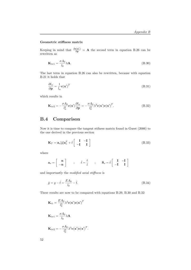
Appendix B

Geometric stiffness matrix

Keeping in mind that ∂c(x′)∂p

= A the second term in equation B.26 can berewritten as

Ktσ1 =σA0

l0λA. (B.30)

The last term in equation B.26 can also be rewritten, because with equationB.21 it holds that

∂ln∂p

=1

lnc(x′)

T(B.31)

which results in

Ktσ2 = −σA0

l2nc(x′)

∂ln∂p

= −σA0


T. (B.32)

B.4 Comparison

Now it is time to compare the tangent stifness matrix found in Guest (2006) tothe one derived in the previous section

KT = as[g]aTs + t

[

I −I

−I I

]

(B.33)

where

as =

[

n

−n

]

; t =t

l; Ss = t

[

I −I

−I I

]

and importantly the modified axial stiffness is

g = g − t =EA0

l0− t. (B.34)

These results are now to be compared with equations B.29, B.30 and B.32:

Kt1 =EA0


T

Ktσ1 =σA0

l0λA

Ktσ2 = −σA0


T.

52


Bearing in mind equation B.25, λ = l0ln

, the equations become

Kt1 =EA0

l0l2nc(x′)c(x′)

T(B.35)

Ktσ1 =σA0

lnA (B.36)

Ktσ2 = −σA0

l3nc(x′)c(x′)

T. (B.37)

When using equation B.23, c(x′) = lnas, these can be rewritten into

Kt1 =EA0

l0asa

Ts (B.38)

Ktσ1 =σA0

lnA (B.39)

Ktσ2 = −σA0

lnasa

Ts . (B.40)

Finally, when it is observed that σA0

lnis equal to t and using g = EA0

l0the

equations can be rewritten as:

Kt1 = as[g]aTs (B.41)

Ktσ1 = tA (B.42)

Ktσ2 = −as[t]aTs . (B.43)

Now it is obvious that Ktσ1 is identical to the stress matrix Ss and when equa-tions B.41 and B.43 are combined they produce the first term from equationB.33.

B.5 Conclusion

Concluding, the two approaches to the tangent stiffness matrix provide identicalresults, given the assumption that the length l in Guest (2006) is equal to thedeformed length ln. This is the case as the bar is assumed to be pretensionedand is thus already in a deformed state.

Unfortunately, most formulations of the tangent stiffness matrix used in tenseg-rity literature are not directly compatible with the formulation using the mod-ified axial stiffness, as they ignore the contribution of equation B.43 due to asmall strain assumption. In the case of zero-free-length springs, that assumptionis no longer valid and the present formulation is required. By introducing the

53

Appendix B

modified axial stiffness, the derivation used in Guest (2006) provides a valuableinsight regarding the use of zero-free-length springs, which is harder to recognizewhen using the traditional FEA approach to the tangent stiffness matrix.

It must be added that the use of a global reference frame makes it easier toarrive at the tangent stiffness formulation mentioned above, compared to theuse of local coordinates on the bars and performing coordinate transformationsat a later stage (Crisfield, 1991, section 3.6).

54

Appendix C

MATLAB Code Description

C.1 Introduction

The main objective of the MATLAB program included on the CDROM is tocalculate the tangent stiffness matrix of a tensegrity structure, and analyse itszero-stiffness modes. The code is commented throughout, and should be self-explanatory for future users reasonably well-versed in the topic. Nevertheless, abrief outline of the code will be given, some custom functions will be discussed inmore detail, and finally, certain noteworthy parts of the code will be highlighted.

C.2 Code outline

The geometry of the tensegrity structure is specified in a separate file, and isdefined by the two structure arrays lmnt and node. The lmnt array containsinformation about element type, node connectivity, stiffness and tension; thenode array contains nodal coordinates.

With these properties of the structure known, the tangent stiffness matrix

is calculated, and its eigenmodes and eigenvalues are investigated. The stiffnessof each of the modes is decomposed into the contributions of the modified ma-terial stiffness matrix and the stress matrix to gain additional insight. As thestructures are modelled free-standing, there are at least 6 rigid-body motions

present in the zero-stiffness modes, which are subsequently removed by meansof a QR-decomposition. The QR-decomposition is further utilized to checkthe linear dependence of the remaining zero-stiffness with the affine trans-

formations of the structure. This numerically verified the developed theoriesconcerning zero stiffness.

Additionally, the program includes the symmetry analysis (Kangwai andGuest, 1999) of a three bar rotationally symmetric tensegrity, which yields thezero-stiffness modes in a symmetry-adapted form. These symmetry-adaptedmodes are then used for performing a small step along the zero-stiffness path,which cannot be solved directly because the stiffness matrix is singular, and thus

55

Appendix C

requires the use of the pseudo-inverse and several iterations until equilibriumis restored.

Limitations

Some remarks regarding the applicability of the code are in order. The code waswritten in tandem with the increasing understanding of zero-stiffness tensegritystructures, and was afterwards rewritten for more general applicability. As aresult the code is not as versatile as one could hope, and it is for instance hard-coded to 3-dimensional structures. The symmetry analysis is written specificallyfor the three bar tensegrity structure and applying the routine to other struc-tures will give nonsensical results. Finally, the path tracking routine (whichaims to follow a zero-stiffness mode) is currently limited to only one step, be-cause the newly calculated equilibrium position is no longer precisely symmetricand the symmetry analysis subsequently returns nonsensical values. This couldbe improved by correcting the intermediate iterations for symmetry, but it wasconsidered beyond the scope of this program.

C.3 Custom functions

[K,S,A,G] = Kt extra(lmnt,node) The Kt extra function calculates the tan-gent stiffness matrix for a structure given by lmnt, node. The functionreturns the various components of the tangent stiffness matrix as used inGuest (2006): the modified material stiffness matrix K, the stress matrixS, the equilibrium matrix A and the modified material matrix G. Thisprovides all the necessary information to fully analyse the stiffness of thestructure. The tangent stiffness matrix is subsequently easily calculatedas Kt = K + S.

drawtens(lmnt,node,‘off’,‘orig’) This function creates a 3-dimensionalimage of the tensegrity given by lmnt, node in the current figure. Ittakes two additional arguments as strings. The first determines whetheror not to plot the element and node numbers, and takes ‘on’ and ‘off’

as values. The second determines whether to plot the structure in itsoriginal or displaced position, respectively indicated by solid and dashedlines, and takes takes the values ‘orig’ and ‘disp’.

displacement vectorplot(node,disp) The nodal displacements of a stiffnessmode can be plotted as a vectors, by using this function. The displace-ments disp are a column vector with xyz displacements for all nodes.The function uses the internal MATLAB function quiver3 to actuallyplot the vectors.

lengths(lmnt,node) This function returns the lengths of the elements, whichis of use for checking the length-preserving properties of the zero-stiffnessmodes.

nodalforces(lmnt,node) This function can be used to check the equilibriumof the tensegrity structure by calculating the resulting nodal forces at eachof the nodes.

56

MATLAB Code Description

C.4 Various remarks

Symmetric tangent stiffness matrix By virtue of its construction, the tan-gent stiffness matrix should be symmetric. In practice this was not alwaysprecisely the case and the analysis would yield complex-valued eigenvalues,which are meaningless in a static analysis. To circumvent this problem,the tangent stiffness matrix is explicitly symmetrized by averaging thesum of Kt and its transpose KT

t .

QR-decomposition An important part in the zero stiffness analysis is playedby the QR-decomposition; among other things it is used to remove therigid-body motions from the zero-stiffness modes. The QR-decompositionis provided by MATLAB and splits up a matrix A in an upper triangularmatrix R of original dimension, and a unitary matrix Q so that A = QR.In practice it makes it possible to identify the linear dependence of variousvectors, by performing a QR-decomposition on the juxtaposed vectors: ifthe resulting R-matrix is a strictly diagonal matrix, all vectors are inde-pendent. If there are off-diagonal elements, there is a linear relationshipbetween the corresponding column vectors in Q.

Tangent space The tangent stiffness matrix is only valid over infinitesimal dis-placements, i.e. the eigenmodes are in tangent space. When the rigid-bodymotions are removed from the zero-stiffness modes, these must thereforealso be in tangent space. In practical terms this means that the con-ventional rotation matrix cannot be used, and that the rotational modesare given by the cross-product of the nodal positions and the unit direc-tion vectors of the principal axes. It can quite easily be verified that thecross product is essentially the same as the derivative of the conventionalrotation matrix, at zero rotation angle.

C.5 Conclusion

The MATLAB program was initially not written as a general purpose FEA

analysis tool for tensegrity structures, but specifically crafted for the analysisof the three bar rotationally symmetric tensegrity structure. In that sense theprogram definitely served its purpose, as it not only provided insights into zero-stiffness structures prior to the development of the underlying theory, but alsoallowed for the verification of the theory by examining specific example struc-tures. The code was later rewritten to accommodate more general functionsand the rewrite resulted in the current form, of which the stiffness section ofthe code can be used for the analysis of any free-standing tensegrity structure.

57

58

Appendix D

Prototype Design

D.1 Introduction

Based on the theory described in Chapter 2, a demonstration prototype wasconstructed. It was built not only to verify the developed theory, and to demon-strate that it is actually possible to physically build these structures, but alsoto get a feel of the challenges that will be encountered when constructing thesesystems.

The design process turned out to be more complex than anticipated, and in-volved the balancing of various conflicting design considerations. A major issuewas the fact that gravity is not taken into account in the theory, and the struc-ture was therefore to be limited in size to minimize the effect of the mass of thestructure. On the other hand, various other constraints provided a lower boundto the dimensions of the structure.

This appendix will describe the design process of the prototype, by first outliningthe conceptual design in Section D.3, and subsequently detailing the final designin Section D.4. The latter chiefly involved establishing suitable dimensions tofit the components, and still obtain a sufficient range of motion. Section D.5provides a brief evaluation of the final design, as well as some pictures of theprototype.

D.2 Design requirements

An important purpose of the prototype is to demonstrate the mechanism-likeproperties of this class of structure. Consequently the range of motion was (qual-itatively) required to be ‘sufficiently large’ to clearly visualize those properties.Actually quantifying the desired range of motion proved to be so intertwinedwith the dimensions of the structure, that it was not considered until the spec-ification of the dimensions in Section D.4.

A major requirement for the prototype is easy adjustment of the parameters,so that the balancing properties can be tuned. This translates into adjustable

59

Appendix D

Figure D.1: Three bar rotationally symmetric tensegrity structure used for theprototype; when all cables are replaced by zero-free-length springs the structureis statically balanced.

attachment points for the springs and wires, as well as some control over thefriction in the system. On one hand the aim was to reduce friction as far aspossible, in order to get as close as possible to a true zero-stiffness structure.On the other hand, some control over friction would be needed to overcome theeffects of gravity forces.

D.3 Prototype description

The structure chosen for the prototype was the three bar rotationally symmetrictensegrity structure shown in Figure D.1. Not only is this structure instantlyrecognizable to people working in the field of tensegrities and often used asa module for larger structures, it also has relatively few components, whichsimplified the design and construction process.

D.3.1 Conceptual design

For the static balancing of the tensegrity structure, the use of springs with a zerorest length is a condition sine qua non. However, the prototype does not actuallyfeature pretensioned zero-free-length springs, and their properties are emulatedby means of regular non-pretensioned springs. This choice is motivated bythe manufacturing difficulties of zero-free-length springs, and the physical restlength of the springs which would unnecessarily limit the range of motion of thestructure. The properties of the zero-free-length spring are emulated by runningthe wire over the endpoint of the bar, to a conventional spring (Herder, 2001).By correctly choosing the total wire length, the spring will be at its rest lengthwhen the endpoint of the wire coincides with the endpoint of the bar, and thusthe tension will be proportional to the ‘length’ of the wire between the two barsit connects.

This translates into a design (schematically shown in Figure D.2) where wiresrun over a yarn guide on the endpoint of the bar, wrap around a pulley attachedto the spring, and are fixed at a flange. This pulley construction halves thenecessary elongation of the spring, so the springs would actually fit on the bar.

60

Prototype Design

Figure D.2: Conceptual design of the bars of the tensegrity structure. Onlyone spring is shown, but two more are attached in similar manner, along thecircumference of the flanges. Two springs (vertical and horizontal) are attachedon one end, and one (horizontal) on the other. Note that this image is not toscale.

Figure D.3: The prototype with the springs corresponding to a single bar; thisis identical for each of the three bars. The angles under which the springs areattached around the bar circumference are determined in Section D.4.

The other end of the wire is attached to a small pin inside the bar. As thetotal structure consists of three bars and nine springs (three horizontal andsix vertical), each bar therefore has three springs attached: a ‘horizontal’ and‘vertical’ spring on one end, and a ‘horizontal’ on the other (see Figure D.3).

Spring design

Unlike many spring applications, the precise spring stiffness was not relevant, asthe springs balance eachother out. A crucial property of the springs, however, isthe required spring stiffness ratio between the horizontal and vertical springs ascalculated in section A.6: the vertical spring must be

√3 times stiffer than the

horizontal spring. What is more, most off-the-shelf springs are pretensioned tosome degree. This would unnecessarily complicate the assembly of the structure,as the levels of pretension would have to be taken into account for the requiredwire length. The combination of these factors led to the decision to custommake the springs without pretension.

As the springs are custom made, further specific requirements could be madeto the ends of the springs to facilitate the design of the total prototype (see

61

Appendix D

Figure D.4: Spring design: one end has a small teflon wheel attached, theother end a threaded rod for adjustability. The endpoint wires are twistedorthogonally to eachother.

Figure D.4). On one end a small threaded rod is attached to the spring, makingadjustment of the spring position possible. The other end of the spring is twistedorthogonally to the spring body, so the pulley (a grooved teflon wheel) candirectly be attached.

Adjustability

The structure can be tuned quite easily by adjusting the position of the spring,as well as the attachment of the wire, with respect to the flanges. This dualadjustability makes rough (spring attachment) and fine (wire attachment) ad-justment possible. All adjustments are made by simply turning a nut.

D.4 Design detailing

This section describes the detailing of the final prototype design. First the bardimensions are determined (with special attention to the range of motion of thestructure), before the other components are described and finalized.

D.4.1 Range of motion

All calculations on the range of motion are performed using the equilibriumequations as found in Appendix A, based on the assumption that the structureis deformed in its fully symmetric zero-stiffness mode and remains symmetricthroughout its deformation. The working range of the structure is then expressedin terms of a generalized parameter, the ratio between height h and radius rof the structure: h/r. It is very difficult to define a ‘sufficient’ h/r range ofmotion, but some idea will be given in the following section.

D.4.2 Bar dimensions

Bar length

Establishing the bar length involved balancing various factors. An upper boundwas given by the increased weight of the structure, and although this was notquantified, it meant that the objective was to minimize the size of the structure,but at the same time maintain a sufficient range of motion. The range of motionis limited by a variety of factors. These factors will be discussed in detail, andby means of Figures D.11 to D.19 the constraints were translated into a suitablechoice of bar length.

62

Prototype Design

10mm + 78% + 10mm

function of flange diameter

Figure D.5: Trade-off of design dimensions. The minimum required distance be-tween the flanges conflicts with the desired distance of the flange to the endpointto avoid contact between the flange and the wires.

spring length + elongation As can be seen in figure D.12, the maximumspring elongation is 47% of the bar length, and assuming that is at 150%elongation, the spring rest length is 31% and the total spring length atmaximum elongation is 78% of the bar length. This determines the mini-mum distance between the flanges, along with some ‘dead’ length for thespring attachment and flange width. The latter was estimated at 10mm ateach end. The above calculation implicitly uses another constraint, thatof the maximum possible spring elongation of 150%. If that value can-not be reached, a larger distance is required between the flanges to reacha similar range of motion, which conflicts with the wire/flange clearancediscussed further down.

wire length The wire length maximally reaches a value of 98% of the barlength (see Figure D.11) and when the spring is fully at rest length thatlength of wire should fit on the bar. As the wire is halved by the pulley,that requires 98/2=49% of the bar length, and with the spring rest lengthof 31% that totals to about 80%. The distance from the endpoint ofthe bar to the flange should be subtracted from that percentage, as somewire length is stored there as well. As a result, the 78% flange distancedescribed above seems to be sufficient.

bar clearance During displacement, the bars with the springs might toucheachother. The likelihood can be reduced by choosing the total diameter ofbar and springs as small as possible, but nevertheless a minimum clearancebetween the bars is required, in order to obtain a certain working range.The minimum required bar clearance is calculated at 30mm from heart toheart of the bars, working on the assumption that both the spring and bardiameter are 10mm, and that they lie side by side. That yields a certainworking range, as can be found in Figure D.16, which is mostly limited inthe lower end of the h/r ratio range.

flange and wire clearance During displacement the wires of the structuremight collide with the flanges to which the spring and wires are attached;thus limiting the range of motion. The flanges couldn’t be moved awayfrom the endpoint indefinitely to avoid contact, as that would conflictwith the minimum required distance between the two flanges. Another

63

Appendix D

LvirtualL

α

Figure D.6: Virtual length and angle assumption in calculations.

approach would be to reduce the diameter of the flange, but that is deter-mined by the diameter of the spring.

The angle between bar and wire is plotted in Figure D.17, and this wasused to create Figure D.19 which shows the required distance of the flangefrom the endpoint, for three different flange radii. The available endpointlength of three bar lengths was also plotted: that is 11% of bar lengthminus 10mm of ‘dead’ length required for spring attachment.

NB: Some notes are in order with regard to this calculation, as it impliesa false sense of accuracy. First of all, because the wires exit from an offsetdue to the bar diameter, there is a ‘virtual’ bar length, which should reallybe used for calculations of the angle. Secondly, the angle is taken from theheart line of the bar, and that is also how the required endpoint distance iscalculated (see Figure D.6). These effects have conveniently been ignored.

Let us first summarize the above described constraints, before they are trans-lated into a choice of bar length:

• minimum required flange distance of 78% plus a ‘dead’ length of 20mm;

• an estimated required clearance of 30mm;

• an estimated required flange radius of ∼15mm.

Using Figure D.16 and D.19, and with the consideration that a sufficient rangeof motion would be h/r = [0.5 . . . 4], we find a bar length of 450mm, providedthe flange radius is maximally 15mm. This h/r ratio can be translated intoa practical height and radius range by means of Figure D.14. When realizingthat the width of the structure is roughly

√3R, that translates into a height

range of 110 . . . 410mm, and width range of 175 . . . 390mm for a bar length of450mm. This range of motion was deemed sufficiently large to visualize themechanism-like properties of the system.

Bar diameter

Based on the available diameter yarn guides in the ascotex catalogue, thedecision was made to use bars with an inner diameter of 6mm, which corresponds

64

Prototype Design

to an inner diameter of about 3.2mm for the yarn guide; this was deemedsufficient to guide three wires through. Next was the choice of material andwall thickness of the tube. Two options are compared in Table D.1.

Table D.1: Comparison of two bars; aluminium and steel with different wallthickness.

Steel Aluminium

Density (kg/m3) 7900 2700Young’s modulus 200E+09 70E+09

Bar properties

Inner (m) 0,006 0,006Outer (m) 0,007 0,008Length (m) 0,450 0,450Weight(kg) 0,036 0,027

Critical Load

Inertia 5,42E-011 1,37E-010Pcr(N) 528 468

With the inner diameter fixed at 6mm, the two options were steel and aluminiumwith respectively a wall thickness of 0.5 and 1mm. The weight and Euler buck-

ling load were calculated for a bar length of 450mm with Pcr = π2EIL2 . The

aluminium bar has a slightly lower buckling load, but is about a third lighter,and was therefore chosen. Note that the axial stiffness of the bars is irrelevantas the lengths will remain constant throughout the displacement.

D.4.3 Springs

Some aspects of the spring design were already discussed in Section D.3, such asthe spring stiffness ratio of

√3, and the wish for the springs to be untensioned.

Several more aspects had to be taken into consideration when designing thedefinitive springs: a maximum allowed spring stiffness is imposed by the bucklingload of the bar, and the springs have to be able to extend at least 150% of theirrest length.

Maximum stiffness

To calculate the maximum spring stiffness in order not to exceed the bucklingload of the bar, a relatively large safety factor of 10 was taken to take intoaccount excentric loading. This provides an upper bound for the forces thatcan be exerted by the spring on the bar. Using Figure D.15 and with thevertical spring stiffness

√3 times higher than the horizontal spring stiffness, the

maximum exerted (normalized) force on the bar (with two horizontal and onevertical spring) can be found at h/r = 1.7. At that point the elongation of all thesprings is approximately 34% of the bar length (see Figure D.12). That meansthat the maximum spring stiffness may not exceed 47N

0.34·450·(2+√

3)= Khor =

0.082N/mm for the horizontal spring.

65

Appendix D

Spring elongation

The allowed spring elongation is closely linked to the dimensions and materialproperties of the spring. The springs used in the structure were individuallymade to specification, by cutting the required length from a long strand ofuntensioned spring with an outer diameter of 10mm, and respectively a wirethickness of 1mm and 0.9mm for the vertical and horizontal spring. The springmaterial was stainless steel.

To see whether the springs could reach the desired elongation of 0.47 · 450 =212mm, a back-of-the-napkin calculation was done, using the formulas and datatables from a spring manual (Verenfabriek Bakker, Hengelo). Input require-ments were that the spring is untensioned, the coils are touching and the springrest length including end attachments is maximally 31% of the bar length.

The relevant spring properties for calculating the spring stiffness, are:

• d = wire diameter

• D = spring diameter (centre to centre; Douter − d)

• n = number of coils

• G = material shear modulus

The spring stiffness as a function of the spring properties is then given as

K =Gd4

8nD3. (D.1)

The decisive question is whether the spring is capable of the desired elongation∆l, as established previously. This can be determined by calculating the springforce at maximum elongation, Fmax = K ·∆l, and comparing the correspondingstress τmax with the maximum allowed values from literature. The τmax is givenby

τmax =8FmaxDk

πd3(D.2)

where k is the Gohner correction factor given by

k = 1 +5

4

1

W+

7

8

1

W 2+

1

W 3

with W the spring index W = D/d. The allowed τmax was further correctedfor the load ratio and number of load cycles. The load ratio is given by theworking range of the spring divided by the maximum force, in our case (Fmax −0)/Fmax = 1, and with a maximum number of load cycles chosen to be 5000,the correction factor was 1.09.

With the above formulas and boundary conditions, the two springs in TableD.2 were calculated. At maximum elongation both springs remain within themaximum allowed stress. These theoretically calculated springs were used asguidelines when actually making the springs from a long strand.

66

Prototype Design

Table D.2: Calculated values for the required springs.horizontal spring vertical spring

body length (mm) 126 128coils 140 128

stiffness (N/mm) 0.0556 0.0958

D.4.4 Yarn guides

The yarn guides were ordered at Ascotex Ltd., and the chosen material typewas T27C, a very smooth titania ceramic. Two different parts were ordered: theflanged eyelet E120 (D1=6mm, d=3.2mm, H=8mm, D2=7.90mm, h=6.20mm),and the tube eyelet TE3 (A=6mm, B=3.5mm, h=6mm).

D.4.5 Wires

For visual effect, as well as reduced friction, the wires were chosen to be asthin as practically possible. Two requirements were placed on the materialproperties: a high stiffness (so that the length does not change significantly withthe changing internal tension during displacement) and the absence of creep, sothat the length actually remains fixed under a constant load. Eventually Kevlarfishing line was used, and because the applied load was much lower than themaximum possible load, the small amount of creep was deemed insignificant.

D.4.6 Pulleys

The pulleys were constructed as simple as possible, and consist of a smallgrooved PTFE (Teflon) wheel, which runs directly around the spring loop.

D.4.7 Flanges

The outer diameter of the flanges was established during the calculation of therequired bar length, and was set at 30mm. A next question was under whichangles to attach the springs around the circumference of the bar. The anglesbetween the springs can be seen in Figure D.7, and their relation to h/r isplotted in Figure D.20. The initial configuration was, somewhat arbitrarily,chosen to be where the angles are approximately at their midpoint between thevalues at h/r=0.5 and 4. This is denoted by the vertical line in Figure D.20,and gave the following angles for spring attachment: 90, 125 and 145. Asthe angles will change during the displacement, it is very likely that the barswill rotate slightly along their axis.

67

Appendix D

-1

-0.8

-0.6

-0.4

-0.2

0

0.2

0.4

0.6

0.8

1

-1-0.8

-0.6-0.4

-0.20

0.20.4

0.60.8

1

0

0.5

1

1.5

2

vertical

lower horizontal

upper horizontal

Figure D.7: View along the axis of a bar, showing the angles between the variouswires connected to the bar. The detail shows the springs on the bar, and thecorresponding wires.

68

Prototype Design

Figure D.8: Overview of range of motion of demonstration prototype, deformedin the symmetric zero-stiffness mode.

D.5 Design Evaluation

Several pictures of the prototype are given in Figure D.8 to D.10, showing severalstages of the assembly process, and providing an indication of the working rangeof the final structure. A major issue in the model is the high level of friction,which is much greater than anticipated, and which reduces the feeling of ‘zero’stiffness. It does serve a useful purpose by compensating for the gravity forces,which had not been taken into account for calculations.

D.5.1 Design process

In retrospect the numerical analysis of the range of motion was too detailed,and too optimistic. The various constraints discovered in the analysis provedto be much less significant than the practical problems posed by the actualcomponents and complexity of assembly. Nevertheless, the analysis did providea great deal of valuable insight in the structure, and it is definitely a necessaryand worthwhile aspect of the design process.

D.5.2 Design and Components

The demonstration prototype has quite a lot of friction, which will have to bereduced in future designs. The use of roller bearings for the pulleys will bean improvement, but the main bottleneck is the tight curvature of the wiresat the endpoint of the bars. The friction currently makes the spring and wireadjustment possibilities redundant, but it will become relevant when the frictionhas been reduced sufficiently.

The three (stiffer) vertical springs proved to be hard-pressed to reach the de-sired 150% elongation, and for a next prototype it would be worthwile to paymore attention to the design of the springs, and to consider more combinations

69

Appendix D

of spring diameter and wire thickness to find a suitable spring. Also, a differentattachment method for the springs would be advisable, which would allow somecontrol over the stiffness of the spring, e.g. a threaded cylinder which can bescrewed into the spring. Thirdly, the current method of attaching the pulleysdoes not scale up well for higher loads, as the spring loop deforms under increas-ing load and consequently the wires often slip out of the grooves. This limitsthe range of motion slightly.

Finally, in the prototype springs without pretension were used in order to facil-itate assembly. It would also be possible to use pretensioned springs, and theywould reduce the required distance between the flanges as less extension wouldbe needed to reach the same tension. On the other hand, the pretension willreduce the range of motion, as the force/displacement curve is cut off sharplywhen the spring reaches its rest length. It is nevertheless worthwile to considerthe use of standard pretensioned springs in future designs.

D.5.3 Assembly

The assembly of the structure is a fairly complex and tedious job. The tedious-ness largely results from having to individually measure the spring propertiesand the required wire lengths. Also, attaching the wires inside the bars, and‘threading’ the wires through the yarn guides, is a fiddly job. The complexitylies in the fact that all bars need to be firmly fixed when tensioning the springs,as the structure is out of balance until all springs are attached. If there is lessfriction in the system, the structure will have to be finetuned to be precisely inbalance, and it will be a difficult task to determine which of the springs has tobe adjusted.

D.5.4 Conclusion

Although the prototype serves its purpose as a proof of concept, it clearly showsthat a lot of work lies ahead, before these types of structures can be put topractical use. Especially the friction has to be reduced drastically to obtain afeeling of zero stiffness. The design process further showed that a thoroughanalysis of the desired range of motion is advisable, not only to determinethe required spring elongations, but also to determine the dimensions of thecomponents of the structure.

70

Prototype Design

(a) When all springs are attached and allwirelengths are measured out, the bars arefirmly fixed with clamps . . .

(b) . . . so that the springs can be tensionedone by one.

(c) Close-up of springs during assembly. (d) Removing the clamps that fix the bars.

(e) Removing last clamp.

Figure D.9: The assembly process involved fixing the bars tightly at a giveninitial position, in order to tension the springs one by one. Once all springs aretensioned, the structure is in equilibrium and the clamps can be removed.

71

Appendix D

(a) Low position (b) Medium position

(c) High position

Figure D.10: Prototype deformed in symmetric zero-stiffness mode. It can bedeformed into a wide range of other shapes as well, as there are two additionalanti-symmetric zero-stiffness modes.

72

Prototype Design

0 0.5 1 1.5 2 2.5 3 3.5 4 4.5 50

1

2

3

4

5

6

1.6529

ratio h/r

ratio

bar length/radius

vertical length/bar lengthhorizontal length/bar length

horizontal length/vertical length

Figure D.11: Lengths of members, versus the h/r ratio. The vertical line indi-cates where the horizontal and vertical wires are of equal length.

0 0.5 1 1.5 2 2.5 3 3.5 4 4.5 50.1

0.15

0.2

0.25

0.3

0.35

0.4

0.45

0.5

ratio h/r

ratio

horizontal elongation/bar length

vertical elongation/bar length

Figure D.12: Spring elongation as ratio of bar length, versus the h/r ratio. Thisis essentially just half of the length of the corresponding wires, plotted in FigureD.11, but zoomed in for better judgement of the values.

73

Appendix D

0.5 0.6 0.7 0.8 0.9 1 1.1 1.2 1.3 1.40

0.5

1

1.5

2

2.5

3

3.5

4

4.5

radius

heig

ht &

ratio

height

height/radius

Figure D.13: Height and radius (ratio) during displacement with constant barlength. This graph makes it possible to read the physical working range of thestructure, once the h/r working range is known.

0.5 0.6 0.7 0.8 0.9 1 1.1 1.2 1.3 1.40

0.5

1

1.5

2

2.5

3

3.5

4

4.5

radius

heig

ht &

ratio

height

height/radiush/r max

h/r min

r min r max

h max

h min

Figure D.14: Height and radius (ratio) during displacement with constant barlength. This example shows how the working range of h/r can be translatedinto height and radius; the h/r working range of 0.5 . . . 4 translates into h =0.6 . . . 2.3 and r = 0.57 . . . 1.28. These values have to be multiplied with a scalingfactor to obtain the actual displacement of the prototype.

74

Prototype Design

0 0.5 1 1.5 2 2.5 3 3.5 4 4.5 5

1.14

1.16

1.18

1.2

1.22

1.24

1.26

ratio h/r

norm

ailz

ed fo

rce

Figure D.15: Normalized bar forces due to spring elongations. The maximumforce is compared with the buckling load of the bar.

0 0.5 1 1.5 2 2.5 3 3.5 4 4.50

0.05

0.1

0.15

0.2

0.25

0.3

0.35

0.4

h/r

Nor

mal

ized

dis

tanc

e be

twee

n ba

rs

1.3226

400

450500

Figure D.16: The normalized clearance between the bars, versus the h/r ratio.The horizontal lines show the 30mm clearance line for various bar lengths, andallows the judgement of working range.

75

Appendix D

0 0.5 1 1.5 2 2.5 3 3.5 4 4.510

20

30

40

50

60

70

80

h/r

angl

e be

twee

n st

rings

and

bar

vertical

horizontal

Figure D.17: Angle between the bar and the horizontal and vertical wires, versusthe h/r ratio.

0 0.5 1 1.5 2 2.5 3 3.5 4 4.50

10

20

30

40

50

60

400

450

500

h/r

Dis

tanc

e fro

m e

ndpo

int f

or ra

dius

of 1

4 to

16m

m

vertical

horizontal

Figure D.18: Required distance from endpoint for various flange diameters. Thehorizontal lines show the available endpoint length, as in 11% of bar length -10mm.

76

Prototype Design

00.5

11.5

22.5

33.5

44.5

0 1 2 3 4 5 6

400

450

500

h/r

Required distance from endpoint for radius of 14 to 16 mm

vertica

l

horizo

nta

l

16m

m

14m

m

Figure D.19: Enlarged version of Figure D.18.

77

Appendix D

0 0.5 1 1.5 2 2.5 3 3.5 4 4.50

20

40

60

80

100

120

140

160

180

ratio h/r

angl

e be

twee

n sp

rings

on

bars

(deg

)

angle lower/vertical

angle upper/ lowerangle upper/vertical

Figure D.20: The angles between the wires on the bar during displacement.This is used to find an initial configuration for the spring attachment on thebars.

78

Appendix E

Zero Stiffness Examples

E.1 Introduction

Several tensegrity geometries with zero-free-length springs as tension membershave been numerically analysed for zero stiffness, using the matlab programdescribed in Appendix C. These include the famous ‘babytoy’ tensegrity, aswell as several rotationally symmetric tensegrities.

For the first, the equilibrium configuration is derived in Section E.2, and for thelatter the equilibrium equations from Appendix A are used; the naming schemeis that of Hinrichs (1984). The structures are plotted in Figures E.2 to E.4, andan overview of the number of zero-stiffness modes in each of the structures isgiven in Table E.1.

Structure No. of bars on conic No. of zero-stiffness modes

‘Babytoy’ 3 3P3(1, 1) 3 3P4(1, 1) 4 2P5(1, 1) 5 1

Table E.1: Structures analysed for zero-stiffness in this section. The numberof zero-stiffness modes and the number of bar directions lying on a conic arelisted, and they correspond to the theory described in Chapter 2.

E.2 ‘Babytoy’ equilibrium

The ‘babytoy’ tensegrity consists of 6 identical bars, divided into three orthog-onal parallel pairs, connected by 24 cables of equal length. The equilibriumposition is calculated by means of the kinematic form-finding method, whichutilizes the fact that cable lengths reach a minimum at the tensegrity equilib-rium configuration.

With x the distance between two parallel bars of length L, the cable length

79

Appendix E

Lcable is written as

Lcable =

√

(

L − x

2

)2

+(x

2

)2

+

(

L

2

)2

=1√2

√

L2 − xL + x2 (E.1)

and the derivate to bar distance x yields

∂Lcable

∂x=

(2x − L)√L2 − xL + x2

1

2√

2= 0

= 2x − L = 0

which gives the solution x = L2 . Subsequent analysis of nodal equilibrium yields

that the tensions coefficients are related as follows:

tbar =3

2tcable (E.2)

These values were used for calculating the three zero-stiffness modes of thestructure, which are plotted in Figure E.1.

80


-1-0.8

-0.6-0.4

-0.20

0.20.4

0.60.8

1

-1

-0.5

0

0.5

1-1

-0.8

-0.6

-0.4

-0.2

0

0.2

0.4

0.6

0.8

1

727

28

10

12

8

12

x-axis

10

14

4

1

1

2

7

11

5

29

30

18

22

5

6

9

13

23

24

8

16

20

2

3

4

3

17

21

15

19

9

11

y-axis

25

266

z-ax

is

-1.5 -1 -0.5 0 0.5 1 1.5-1.5

-1

-0.5

0

0.5

1

1.5

x-axis

First zero-stiffness mode

z-ax

is

-1.5

-1

-0.5

0

0.5

1

1.5

-1.5-1-0.500.511.5

Second zero-stiffness mode

y-axis

x-ax

is

-1.5 -1 -0.5 0 0.5 1 1.5-1.5

-1

-0.5

0

0.5

1

1.5

y-axis

Third zero-stiffness mode

z-ax

is

Figure E.1: The ‘babytoy’ tensegrity structure. Its three zero-stiffness modesroughly correspond to shear on three orthogonal planes. No symmetrization hasbeen performed on the modes, and it is expected that such an analysis wouldyield perfectly orthogonal shears.

81

Appendix E

-2-1.5

-1-0.5

00.5

11.5

2

-2-1.5

-1-0.5

00.5

11.5

2-1

-0.5

0

0.5

1

1.5

2

2.5

3

x-axis

2

9

4

6

2

1

10

12

4

6

11

3

7

5

3

8

1

5

y-axis

z-ax

is

-2-1.5

-1-0.5

00.5

11.5

2

-2-1.5

-1-0.5

00.5

11.5

2-1

-0.5

0

0.5

1

1.5

2

2.5

3

x-axisy-axis

z-ax

is

-2-1.5

-1-0.5

00.5

11.5

2

-2-1.5

-1-0.5

00.5

11.5

2-1

-0.5

0

0.5

1

1.5

2

2.5

3

x-axisy-axis

z-ax

is

-2-1.5

-1-0.5

00.5

11.5

2

-2-1.5

-1-0.5

00.5

11.5

2-1

-0.5

0

0.5

1

1.5

2

2.5

3

x-axisy-axis

z-ax

is

Figure E.2: A P3(1, 1) structure with its three symmetrized zero-stiffness modes.The first corresponds to a scaling transformation, the latter two are combina-tions of shear and scaling.

82


-2-1.5

-1-0.5

00.5

11.5

2

-2-1.5

-1-0.5

00.5

11.5

2-1

-0.5

0

0.5

1

1.5

2

2.5

3

x-axis

3

8

5

16

8

11

10

5

43

4

13

15

2

12

7

12

9

614

7

6

1

y-axis

z-ax

is

-2

-1.5

-1

-0.5

0

0.5

1

1.5

2

-2-1.5-1-0.500.511.52y-axis

x-ax

is

-2 -1.5 -1 -0.5 0 0.5 1 1.5 2-1

-0.5

0

0.5

1

1.5

2

2.5

3

x-axis

z-ax

is

Figure E.3: A P4(1, 1) structure with its zero-stiffness modes. The first mostlyconsists of a skewing transformation, the second mostly of a scaling transfor-mation.

83

Appendix E

-2-1.5

-1-0.5

00.5

11.5

2

-2-1.5

-1-0.5

00.5

11.5

2-1

-0.5

0

0.5

1

1.5

2

2.5

3

x-axis

4

10

1020

13

6

3

14

5

4

6

19

9

16

12

5

1

3

9

7

2

2

15

18

7

17

11

8

1

8

y-axis

z-ax

is

-2-1.5

-1-0.5

00.5

11.5

2

-2-1.5

-1-0.5

00.5

11.5

2-1

-0.5

0

0.5

1

1.5

2

2.5

3

x-axisy-axis

z-ax

is

Figure E.4: A P5(1, 1) structure with its zero-stiffness mode, which correspondsto a scaling transformation.

84

Appendix F

Future Work

F.1 Introduction

The work described in this MSc. thesis has been a first step in the direction ofa fundamental understanding of zero-stiffness structures. This section brieflydiscusses some possible directions for future research, and where possible, pro-vides some pointers. The limitations imposed by only considering tensegritystructures, namely absence of external forces and constraints, are first to beconsidered, before other issues such as range of motion and practical applica-tions are looked into.

F.2 Future work

external forces The current theory cannot take into account exernal loads, asit makes use of the fact that in unloaded state, affine transformations ofthe nodal coordinates are in the nullspace of the stress matrix. This nolonger holds when there are external loads present.

A priority is to include constant gravity forces in the calculations, andsome possible approaches were considered, but none were carried throughto fruition. The first would be to qualitatively include gravity forces asa special type of ‘gravity element’ with a specific direction and of infi-nite length, which might or might not lie on the conic. The next stepwould then be to say that the affine transformation U should maintainthe direction v of that element, and therefore

U(pi − pj) = Uvij = λvij

and the element direction is thus an eigenvector with eigenvalue λ. Theeigenvalue would be 1 if the ‘gravity element’ lies on the conic, and itslength is therefore preserved.

85

Appendix F

Another (quantitative) approach would be to reconsider the structuralequilibrium as

Ωp = fext

where the effect of the affine transformation U on each of the n nodes,can be written as

ΩU′p = U′fext

= 1 · fext

with U′ = In ⊗U a blockdiagonal matrix with U working on each of thenodal coordinates/forces. As a result, one can see that a constant fext isan eigenvector of the blockdiagonal U′ with eigenvalue 1.

constraints Although traditionally tensegrity structures are analysed as freestanding, in practice some degrees of freedom are fixed in order to removerigid-body motions. The choice of constraints strongly influences the pos-sible deformations of the structure, and therefore the structure needs tobe fixed without prohibiting the length-preserving affine transformationsthat have zero stiffness. It is as of yet unclear how to do this in a generalmanner.

An interesting approach is to first only consider the subset of displace-ments that are length-preserving for the conventional elements. This isdone numerically by means of a QR-decomposition, where the rows of thecompatibility matrix C are orthogonalized in two parts: one that involveselongations of conventional members, and a set Czfl that does not. Withthe latter set, a reduced stiffness matrix can be obtained, which is limitedto only those displacements that are length-preserving for conventionalelements.

Kt,reduced = CTzflKtCzfl

This technique might facilitate finding affine transformations that are notprohibited by the nodal constraints.

non-pin-jointed structures Once the issues of external loads and constraintshave been solved, the question arises whether (some of) the above devel-oped theory can be extended to also include non-pin-jointed structuressuch as the ‘Anglepoise’ lamp, and to confirm and extend the modifica-tion rules developed by Herder (2001).

range of motion Numerical calculation of the zero-stiffness modes producesdisplacements in tangent space. Therefore, for large displacements itera-tive techniques need to be employed to find a next equilibrium configura-tion, even more so because the tangent stiffness matrix is per definitionsingular.

It is therefore very difficult to intuitively extrapolate from the calculatedzero-stiffness modes, to see how it is best interpreted over large displace-ments and what the range of motion would be. For instance consider

86

Future Work

Figure F.1: In tangent space, the zero-stiffness mode of this statically balancedstructure corresponds to shear and scaling, but on macro scale, it correspondsto the rotation of the two bar with respect to each other.

the simple statically balanced structure in Figure F.1; the structure hasa zero-stiffness mode that can numerically be described as consisting ofshear and scaling. However, on a macro level, one can see that the twobars rotate with respect to eachother. The question is, how this can bedone more generally and for more complex (three-dimensional) structures.

An approach to this would be either to analytically analyse the struc-tures, or look at mechanism theory and try to find techniques from thatfield; mechanisms concepts such as the number of Degrees of Freedom ofa mechanism should also be investigated.

practical application The demonstration prototype described in Appendix Dwas constructed not only to demonstrate that these types of structureactually exist, but also to get a feel for the practical issues that arise whentrying to construct zero stiffness tensegrities.

There is a lot more (practical) work to be done here, not only to reducefriction and to device more efficient methods of construction, but alsoto make the structures simpler and more robust, and thus suitable forpractical applications.

overview of zero-stiffness modes As indicated in Chapter 3 there exist typesof zero stiffness which are not yet fully understood, and several examplestructures were given. In order to understand these structures, furtherresearch is needed, with special attention to the presence of unstressednodes.

other forms of zero stiffness Other forms of zero stiffness are described inliterature, such as by Tarnai (2003) where the equilibrium paths at abifurcation point remain neutrally stable over a finite range of motion. Itis currently unclear how these forms of zero stiffness are related to theones described in this research.

sensitivity analysis It would be interesting to analyse the sensitivity of thezero-stiffness modes to perturbations and/or imperfections of initial con-ditions. Will the calculated modes zero-stiffness modes also be present inconfigurations close to the analysed ones; for example if the conventionalmembers do not precisely lie on a conic?

87

Appendix F

F.3 Conclusion

The above suggestions for future work illustrate that only the first steps havebeen taken in fully understanding zero-stiffness tensegrity structures. A lot ofwork is left in the theoretical field, and also (and in common with tensegritiesin general) in practical design and applications. As the applications will mostlikely be based on the mechanism-like properties of the structures, the links tomechanism theory should definitely be explored.

88

Bibliography

Calladine, C. R., 1978. Buckminster Fuller’s ‘tensegrity’ structures and ClerkMaxwell’s rules for the construction of stiff frames. International Journal ofSolids and Structures 14, 161–172.

Calladine, C. R., Pellegrino, S., 1991. First-order infinitesimal mechanisms. In-ternational Journal of Solids and Structures 27 (4), 505–515.

Calladine, C. R., Pellegrino, S., 1992. Further remarks on first-order infinitesi-mal mechanisms. International Journal of Solids and Structures 29 (17), 2119–2122.

Connelly, R., 1999. Tensegrity structures: Why are they stable? In: Thorpe,M. F., Duxbury, P. M. (Eds.), Rigidity Theory and Applications. KluwerAcademic/Plenum Publishers, pp. 47–54.






Crisfield, M. A., 1991. Non-linear Finite Element Analysis of Solids and Struc-tures. Volume 1: Essentials. John Wiley & Sons.







89





Pellegrino, S., 1990. Analysis of Prestressed Mechanisms. International Journalof Solids and Structures 26 (12), 1329–1350.






90

Documents

Theory and Design of Statically Balanced Tensegrity Mechanisms · Tensegrity structures, or tensegrities, are a special type of prestressed pin-jointed bar frameworks with unique