Embed Size (px)
Citation preview
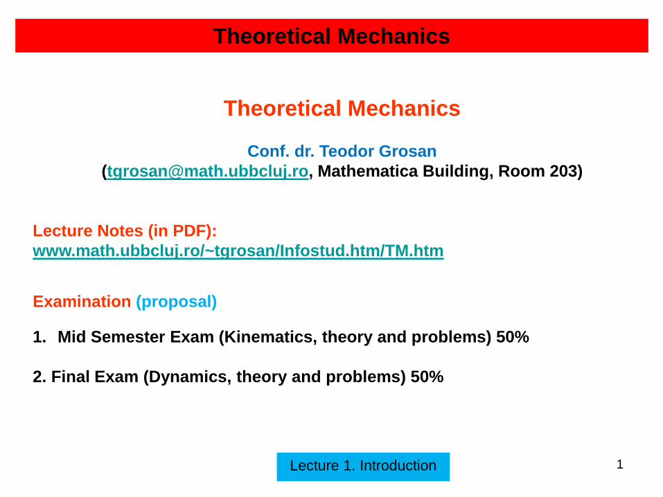
Lecture 1. Introduction 1
Theoretical Mechanics
Theoretical Mechanics
Conf. dr. Teodor Grosan
([email protected], Mathematica Building, Room 203)
Lecture Notes (in PDF):
www.math.ubbcluj.ro/~tgrosan/Infostud.htm/TM.htm
Examination (proposal)
1. Mid Semester Exam (Kinematics, theory and problems) 50%
2. Final Exam (Dynamics, theory and problems) 50%

Lecture 1. Introduction 2
Theoretical Mechanics
References:
1. Kohr, M., Capitole Speciale de Mecanică, Presa Universitară Clujeană, Cluj-
Napoca, 2005.
2. Brãdeanu, P., Mecanică Teoretică, vol. 1 şi 2, Litografia Universităţii Babeş-
Bolyai, Cluj-Napoca, 1988.
3. Iacob, C., Mecanică Teoretică, Editura Didactică şi Pedagogică, Bucureşti, 1980.
4. Dragoş, L., Principiile Mecanicii Analitice, Editura Tehnică, Bucureşti, 1976.
Goldstein, H., Poole, C., Safko, J., Classical Mechanics, Reading, MA: Addison-
Wessley Publ. Co. (3rd edition), 2014.
5. Bose, S., Chattoraj, D., Elementary Analytical Mechanics, Alpha Science
International Ltd. 2000.
6. Aaron, F.D., Mecanică Analitică, Editura BIC ALL, Bucureşti, 2002.
7. Landau, L.D., Lifshitz, E.M., Mechanics, Elsevier-Butterworth-Heinemann, (3rd
edition), 2005.
8. Russo, R., Classical Problems in Mechanics, Aracne, Roma, 1997.
Lecture 1. Introduction 3
Theoretical Mechanics
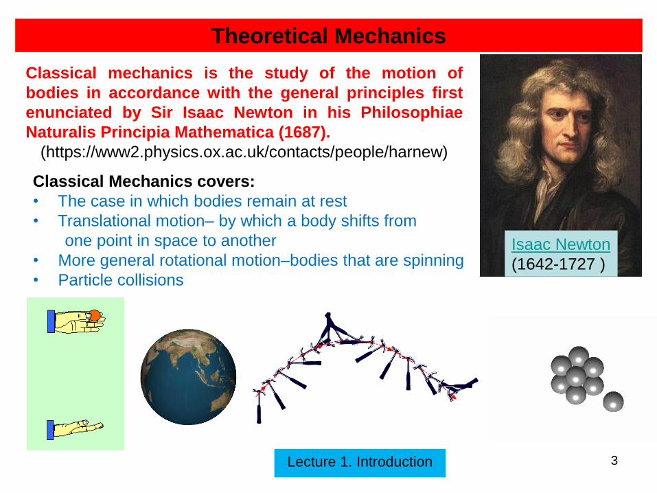
Classical mechanics is the study of the motion of
bodies in accordance with the general principles first
enunciated by Sir Isaac Newton in his Philosophiae
Naturalis Principia Mathematica (1687).
(https://www2.physics.ox.ac.uk/contacts/people/harnew)
Isaac Newton
(1642-1727 )
Classical Mechanics covers:
• The case in which bodies remain at rest
• Translational motion– by which a body shifts from
one point in space to another
• More general rotational motion–bodies that are spinning
• Particle collisions

Lecture 1. Introduction 4
Theoretical Mechanics
Classical Mechanics valid on scales which are:
• Not too fast ( e.g.. high energy particle tracks from CERN)
• v << c = 299 792 458 m/s [speed of light in vacuum]
• If too fast, time is no longer absolute - need special relativity.
Earth-Moon: 384 400 km - 1,282 sec
Lecture 1. Introduction 5
Theoretical Mechanics
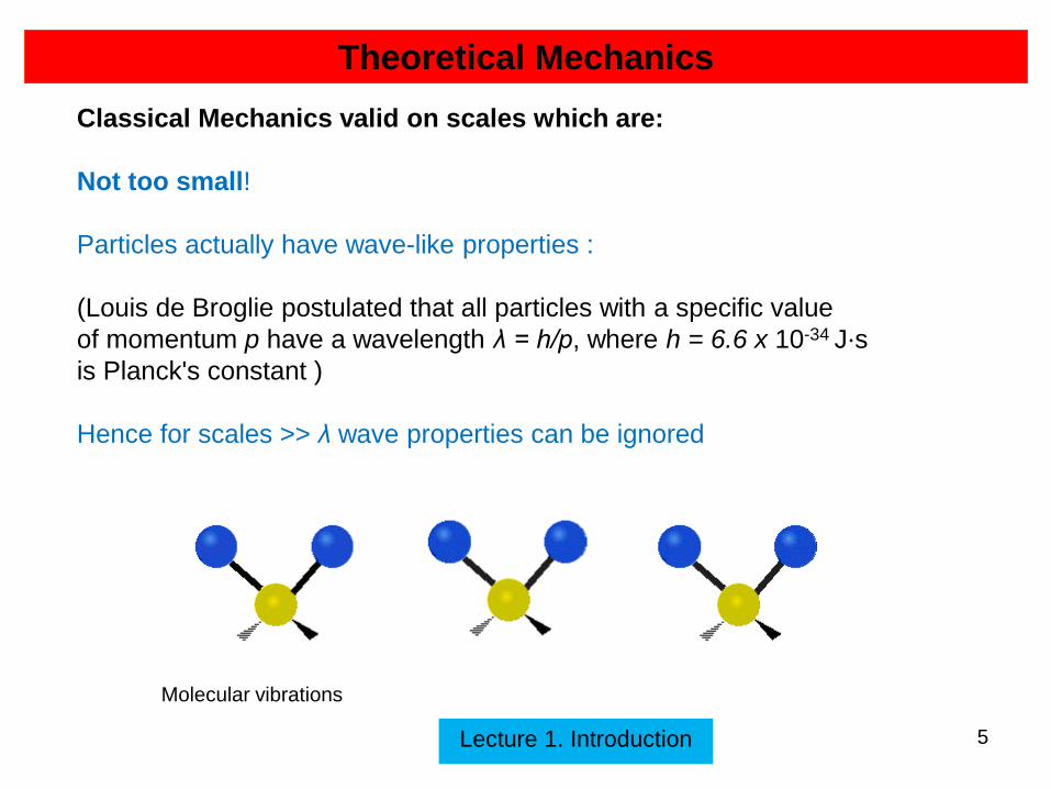
Classical Mechanics valid on scales which are:
Not too small!
Particles actually have wave-like properties :
(Louis de Broglie postulated that all particles with a specific value
of momentum p have a wavelength λ = h/p, where h = 6.6 x 10⁻³⁴ J⋅s
is Planck's constant )
Hence for scales >> λ wave properties can be ignored
Molecular vibrations
Lecture 1. Introduction 6
Theoretical Mechanics
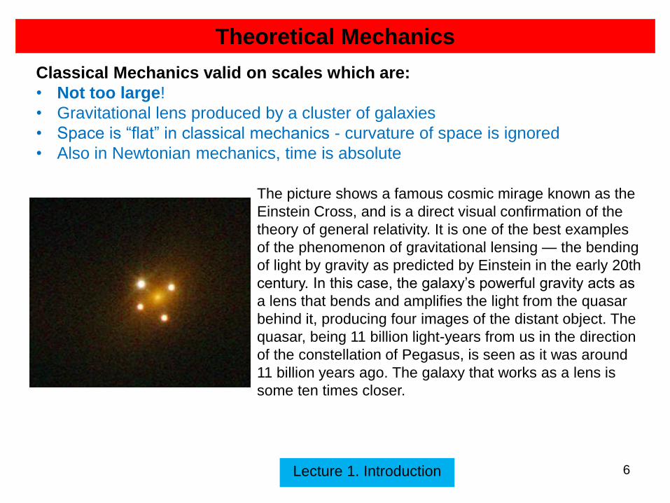
Classical Mechanics valid on scales which are:
• Not too large!
• Gravitational lens produced by a cluster of galaxies
• Space is ―flat‖ in classical mechanics - curvature of space is ignored
• Also in Newtonian mechanics, time is absolute
The picture shows a famous cosmic mirage known as the
Einstein Cross, and is a direct visual confirmation of the
theory of general relativity. It is one of the best examples
of the phenomenon of gravitational lensing — the bending
of light by gravity as predicted by Einstein in the early 20th
century. In this case, the galaxy’s powerful gravity acts as
a lens that bends and amplifies the light from the quasar
behind it, producing four images of the distant object. The
quasar, being 11 billion light-years from us in the direction
of the constellation of Pegasus, is seen as it was around
11 billion years ago. The galaxy that works as a lens is
some ten times closer.
Lecture 1. Introduction 7
Theoretical Mechanics
0. Preliminaries (A. Bettini, A Course in Classical Physics 1—Mechanics, Springer, 2016)
(A. Romano, A. Marasco, Classical Mechanics with Mathematica®, 2nd ed., Birkhaeser, 2012)
The time is the succession of events. The Newtonian time is linear (has a uniform
flow) and irreversible.
Motion of a body means that its position in space varies in time. The notion of
motion is relative: a passenger in a plane sitting in his chair has a fixed position
relative to the plane, but moves at, say 800 km/h relative to a person standing on
earth. The latter moves at 800 km/h relative to the passenger, in the opposite
direction.
To describe the motion we then need a reference frame. Usually, a reference frame
is fixed on the earth. The possible choices are still infinite.
Kinematics is the part of classical mechanics that studies the motion of a body,
ignoring its causes.
Lecture 1. Introduction 8
Theoretical Mechanics
A particle (“material point”) is an object whose size can be ignored in a particular
context.
This abstraction allows to simplify the observation of motion, as it gets rid of the
complications deriving from the extension of real bodies. Moreover this abstraction
is introductory to the far more complex study of real bodies.
Kinematics of the material point studies the motion of a point-like (particle) object.
Lecture 1. Introduction 9
Theoretical Mechanics
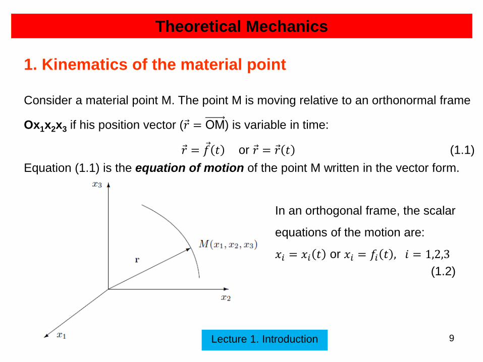
1. Kinematics of the material point
Consider a material point M. The point M is moving relative to an orthonormal frame
Ox1x2x3 if his position vector (𝑟 = OM) is variable in time:
𝑟 = 𝑓 𝑡 or 𝑟 = 𝑟 𝑡 (1.1)
Equation (1.1) is the equation of motion of the point M written in the vector form.
In an orthogonal frame, the scalar
equations of the motion are:
𝑥𝑖 = 𝑥𝑖 𝑡 or 𝑥𝑖 = 𝑓𝑖 𝑡 , 𝑖 = 1,2,3
(1.2)
Lecture 1. Introduction 10
Theoretical Mechanics
If 𝑥𝑖 𝑡 or 𝑓𝑖 𝑡 are known in a time interval 𝑡0, 𝑇 , 𝑡0 > 0; 𝑇 < ∞, then the motion of
the material point M in the frame Ox1x2x3 is known in this time range.
The function
𝑟 : 𝑡0, 𝑇 𝑅3, 𝑟 = 𝑟 𝑡 (1.3)
associates to every moment 𝑡 ∈ 𝑡0, 𝑇 a unique position in space for the point M.
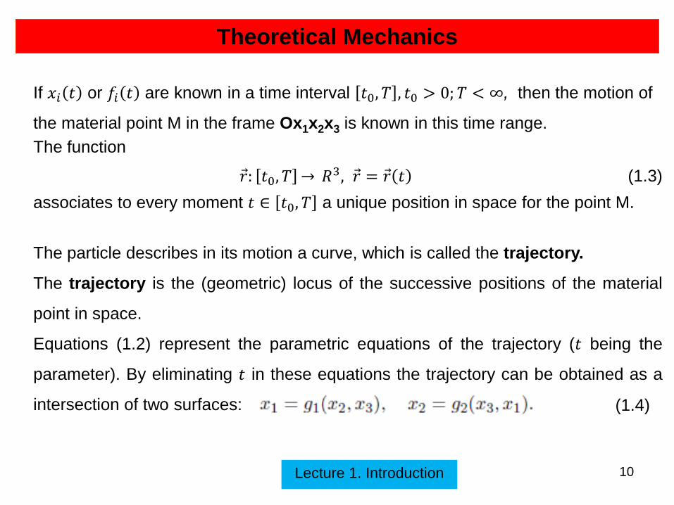
The particle describes in its motion a curve, which is called the trajectory.
The trajectory is the (geometric) locus of the successive positions of the material
point in space.
Equations (1.2) represent the parametric equations of the trajectory (𝑡 being the
parameter). By eliminating 𝑡 in these equations the trajectory can be obtained as a
intersection of two surfaces: (1.4)

Lecture 1. Introduction 11
Theoretical Mechanics
Further, we suppose that 𝑥𝑖 𝑡 are functions of class 𝐶𝑘 (𝑘 ≥ 2) on the motion
interval. Thus, the trajectory is a rectifiable curve* and it is possible to specify the
position of the point M on the trajectory by using an intrinsic coordinate, 𝑠, the arc
length on the trajectory, measured from an initial position 𝑂′ to the current position of
the point M.
Moreover, the parametric representation of
the trajectory (depending on the parameter
s) has the form:
𝑟 = 𝑟 𝑠 , 𝑠𝜖 0, 𝑆 , 𝑆 > 0 (1.5)
In this case, the equation of the motion of
the particle on the trajectory is given by:
𝑠 = 𝑠(𝑡), 𝑡𝜖 𝑡0, 𝑇 (1.6)
* A rectifiable curve is a curve having finite length.
Lecture 1. Introduction 12
Theoretical Mechanics
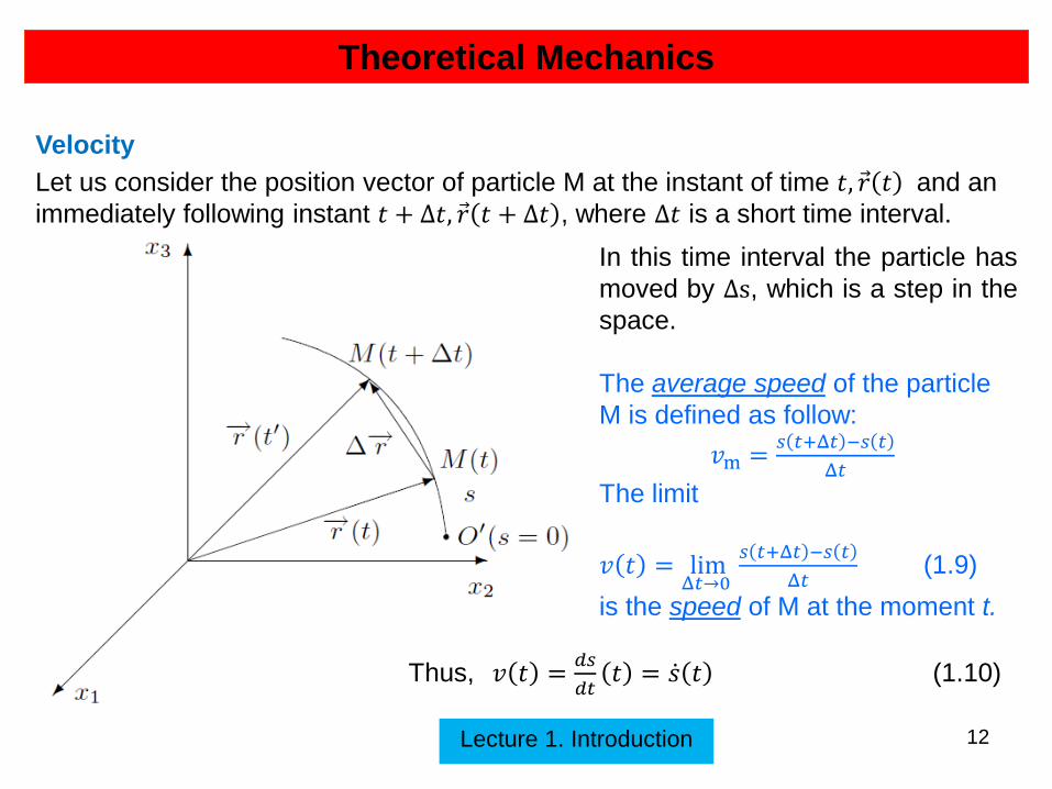
Velocity
Let us consider the position vector of particle M at the instant of time 𝑡, 𝑟 𝑡 and an
immediately following instant 𝑡 + Δ𝑡, 𝑟 𝑡 + Δ𝑡 , where Δ𝑡 is a short time interval.
In this time interval the particle has
moved by Δs, which is a step in the
space.
The average speed of the particle
M is defined as follow:
𝑣m =𝑠 𝑡+Δ𝑡 −𝑠 𝑡
Δ𝑡
The limit
𝑣 𝑡 = limΔ𝑡 0
𝑠 𝑡+Δ𝑡 −𝑠 𝑡
Δ𝑡 (1.9)
is the speed of M at the moment t.
Thus, 𝑣 𝑡 =𝑑𝑠
𝑑𝑡𝑡 = 𝑠 𝑡 (1.10)
Lecture 1. Introduction 13
Theoretical Mechanics
The average velocity in the time interval Δ𝑡 is the vector obtained by dividing the
displacement Δ𝑟 by the time interval in which it happens:
𝑣 m =𝑟 𝑡 + Δ𝑡 − 𝑟 𝑡
Δ𝑡=Δ𝑟
Δ𝑡
The (instantaneous) velocity is the limit for Δ𝑡 0 of the average velocity, namely
𝑣 𝑡 = limΔ𝑡 0
𝑟 𝑡 + Δ𝑡 − 𝑟 𝑡
Δ𝑡
Thus,
𝑣 𝑡 =𝑑𝑟
𝑑𝑡= 𝑟 𝑡 = 𝑥1 𝑡 𝑖 1 + 𝑥2 𝑡 𝑖 2 + 𝑥3 𝑡 𝑖 3 = 𝑣1𝑖 1 + 𝑣2𝑖 2 + 𝑣3𝑖 3
However, we have 𝑟 = 𝑟 𝑠 and 𝑠 = 𝑠 𝑡 and we get
𝑣 𝑡 =𝑑 𝑟
𝑑𝑡=
𝑑𝑟
𝑑𝑠
𝑑𝑠
𝑑𝑡= 𝑣 𝜏
where 𝜏 is the tangent versor (unit vector) at the trajectory in the point M.
(1.11)
(1.12)
(1.13)
(1.14)

Lecture 1. Introduction 14
Theoretical Mechanics
Remark: The velocity vector is tangent to the trajectory, is oriented in the sense of
the displacement and its algebraic magnitude is 𝑠 =𝑑𝑠
𝑑𝑡 .
𝑣 = 𝑠 𝜏
Acceleration
The ratio
𝑎 𝑚 𝑡 =𝑣 𝑡 + Δ𝑡 − 𝑣 𝑡
Δ𝑡
is the average acceleration of the particle M.
(1.15)
(1.16)
Lecture 1. Introduction 15
Theoretical Mechanics
(1.17)
(1.18)
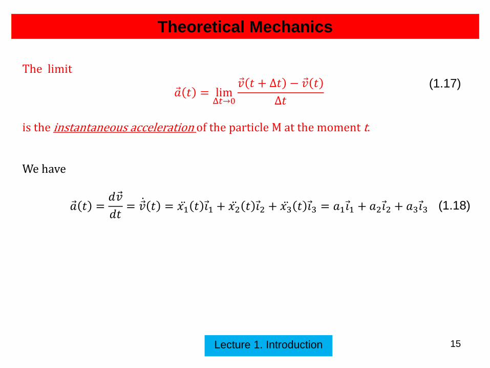
The limit
𝑎 𝑡 = limΔ𝑡 0
𝑣 𝑡 + Δ𝑡 − 𝑣 𝑡
Δ𝑡
is the instantaneous acceleration of the particle M at the moment t.
We have
𝑎 𝑡 =𝑑𝑣
𝑑𝑡= 𝑣 𝑡 = 𝑥1 𝑡 𝑖 1 + 𝑥2 𝑡 𝑖 2 + 𝑥3 𝑡 𝑖 3 = 𝑎1𝑖 1 + 𝑎2𝑖 2 + 𝑎3𝑖 3
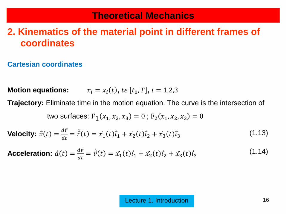
2. Kinematics of the material point in different frames of
coordinates
Cartesian coordinates
Motion equations: 𝑥𝑖 = 𝑥𝑖 𝑡 , 𝑡𝜖 𝑡0, 𝑇 , 𝑖 = 1,2,3
Trajectory: Eliminate time in the motion equation. The curve is the intersection of
two surfaces: F1 𝑥1, 𝑥2, 𝑥3 = 0 ; F2 𝑥1, 𝑥2, 𝑥3 = 0
Velocity: 𝑣 𝑡 =𝑑𝑟
𝑑𝑡= 𝑟 𝑡 = 𝑥1 𝑡 𝑖 1 + 𝑥2 𝑡 𝑖 2 + 𝑥3 𝑡 𝑖 3
Acceleration: 𝑎 𝑡 =𝑑𝑣
𝑑𝑡= 𝑣 𝑡 = 𝑥1 𝑡 𝑖 1 + 𝑥2 𝑡 𝑖 2 + 𝑥3 𝑡 𝑖 3
Lecture 1. Introduction 16
Theoretical Mechanics
(1.13)
(1.14)
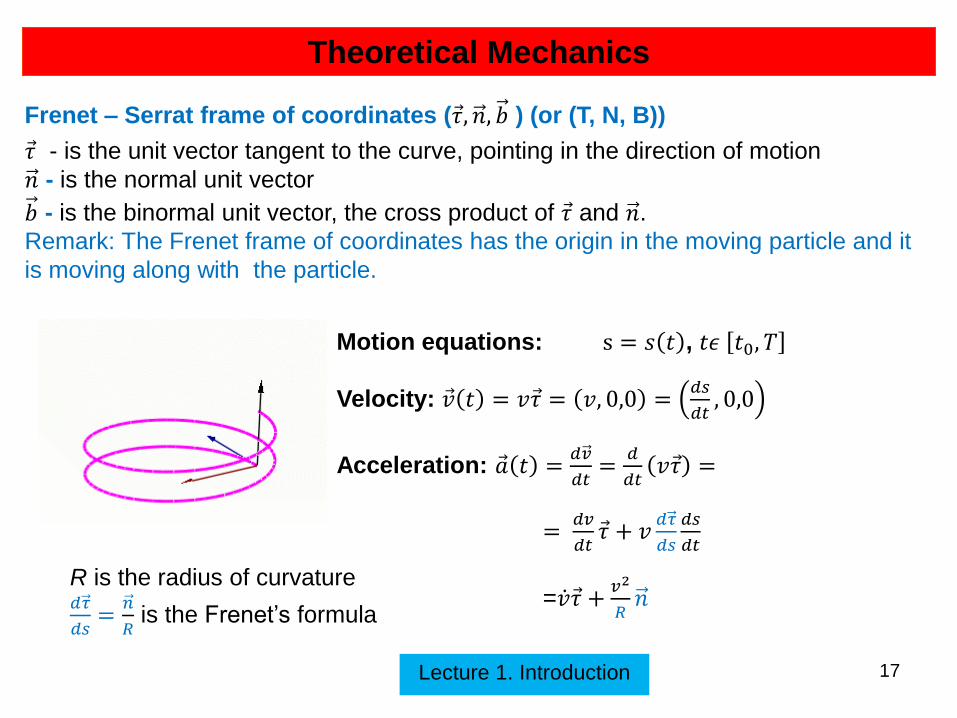
Frenet – Serrat frame of coordinates (𝜏 , 𝑛, 𝑏 ) (or (T, N, B))
𝜏 - is the unit vector tangent to the curve, pointing in the direction of motion
𝑛 - is the normal unit vector
𝑏 - is the binormal unit vector, the cross product of 𝜏 and 𝑛.
Remark: The Frenet frame of coordinates has the origin in the moving particle and it
is moving along with the particle.
Lecture 1. Introduction 17
Theoretical Mechanics
Motion equations: s = 𝑠 𝑡 , 𝑡𝜖 𝑡0, 𝑇
Velocity: 𝑣 𝑡 = 𝑣𝜏 = 𝑣, 0,0 =𝑑𝑠
𝑑𝑡, 0,0
Acceleration: 𝑎 𝑡 =𝑑𝑣
𝑑𝑡=
𝑑
𝑑𝑡𝑣𝜏 =
= 𝑑𝑣
𝑑𝑡𝜏 + 𝑣
𝑑𝜏
𝑑𝑠
𝑑𝑠
𝑑𝑡
=𝑣 𝜏 +𝑣2
𝑅𝑛
R is the radius of curvature 𝑑𝜏
𝑑𝑠=
𝑛
𝑅 is the Frenet’s formula

Thus, we have
𝑎 𝑡 = 𝑣 ,𝑣2
𝑅, 0 = a𝜏𝜏 + a𝑛𝑛
where a𝜏 = 𝑣 is the tangential acceleration and a𝑛= 𝑣2
𝑅 is the normal acceleration.
Lecture 1. Introduction 18
Theoretical Mechanics
In 2D the curvature 𝜌 =1
𝑅 is:
or for

Example: (https://math.libretexts.org/Bookshelves/Calculus/) Without finding T and N, write the acceleration of the motion
Lecture 1. Introduction 19
Theoretical Mechanics
To solve this problem, we must first find the particle's velocity.

Lecture 1. Introduction 20
Theoretical Mechanics
On the other hand
Thus,
A similar problem

21
Theoretical Mechanics
Lecture 1. Introduction
(https://ocw.mit.edu/courses/aeronautics-and-astronautics/)
Lecture 1. Introduction 22
Theoretical Mechanics
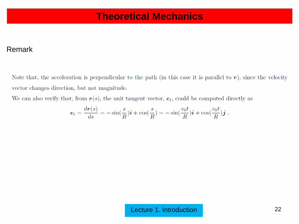
Remark