Embed Size (px)
DESCRIPTION
The Wealth of Nations. Jamie Brabston Matt Caulfield Mark Testa. Overview. Introduction Regression of Individual Variables Multicollinearity Multiple Regression Stepwise Regression Final Model. Introduction. Collected data for 30 countries 12 variables - PowerPoint PPT Presentation
Citation preview

The Wealth of Nations
Jamie BrabstonMatt Caulfield
Mark Testa
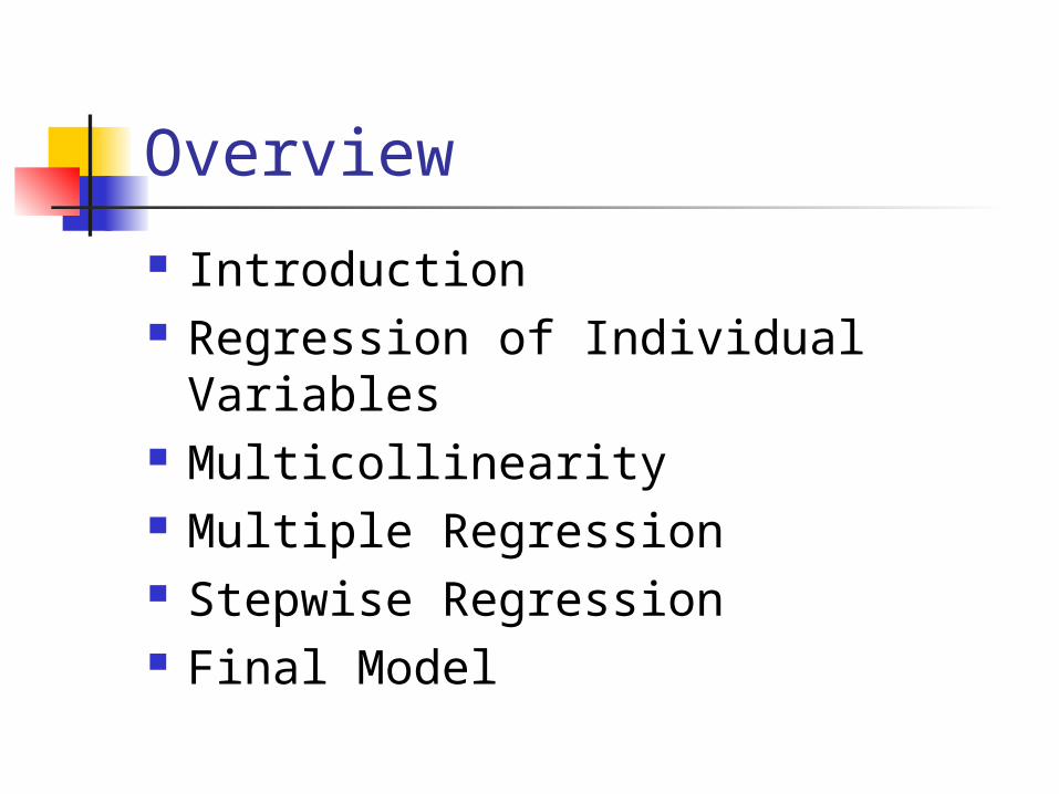
Overview
Introduction Regression of Individual Variables Multicollinearity Multiple Regression Stepwise Regression Final Model
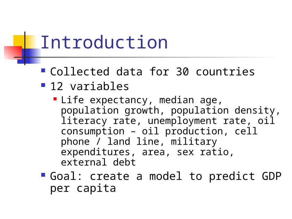
Introduction Collected data for 30 countries 12 variables
Life expectancy, median age, population growth, population density, literacy rate, unemployment rate, oil consumption – oil production, cell phone / land line, military expenditures, area, sex ratio, external debt
Goal: create a model to predict GDP per capita
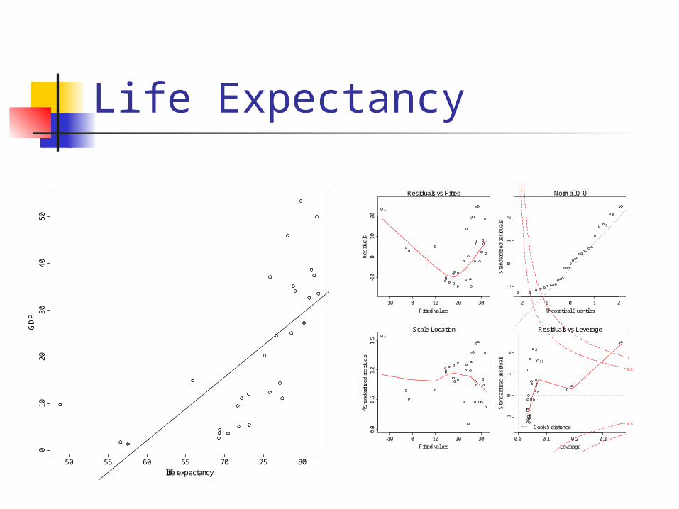
Life Expectancy
50 55 60 65 70 75 80
01
02
03
04
05
0
life.expectancy
GD
P
-10 0 10 20 30
-10
010
20
Fitted values
Res
idua
ls
Residuals vs Fitted
84
6
-2 -1 0 1 2
-10
12
Theoretical Quantiles
Sta
ndar
dize
d re
sidu
als
Normal Q-Q
4
8
6
-10 0 10 20 30
0.0
0.5
1.0
1.5
Fitted values
Sta
ndar
dize
d re
sidu
als
Scale-Location4
8
6
0.0 0.1 0.2 0.3
-10
12
Leverage
Sta
ndar
dize
d re
sidu
als
Cook's distance0.5
0.5
1
Residuals vs Leverage
4
8
11
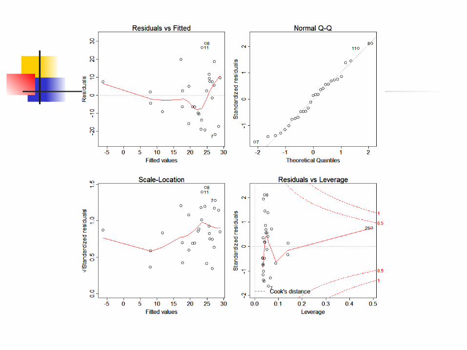
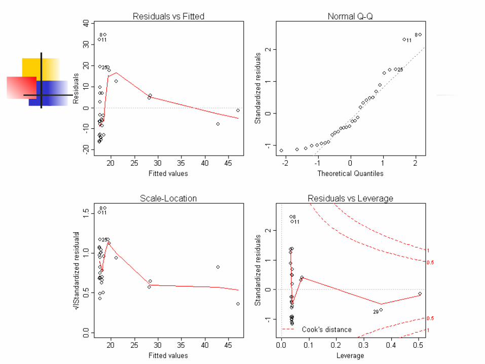
Life Expectancy
Analysis: R2: 0.45. P-value: Highly significant.
An outlier was identified using a Leverage-residual plot and removed.
Residuals vs. Fitted Values plot showed nonlinearity.
Tried a Box-Cox transform.
Life Expectancy
0.0 0.5 1.0 1.5 2.0 2.5
0.0
50
.10
0.1
50
.20
0.2
50
.30
0.3
5
Absolute value of externally studentised residuals
influ
en
ce
1
2
3
4
5
67
8
910
11
1213
14
15
1617
18
192021
22
232425
26
272829
30
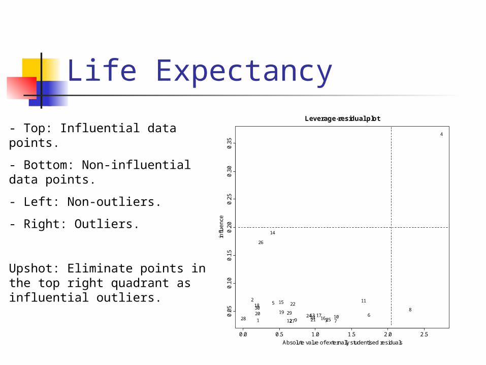
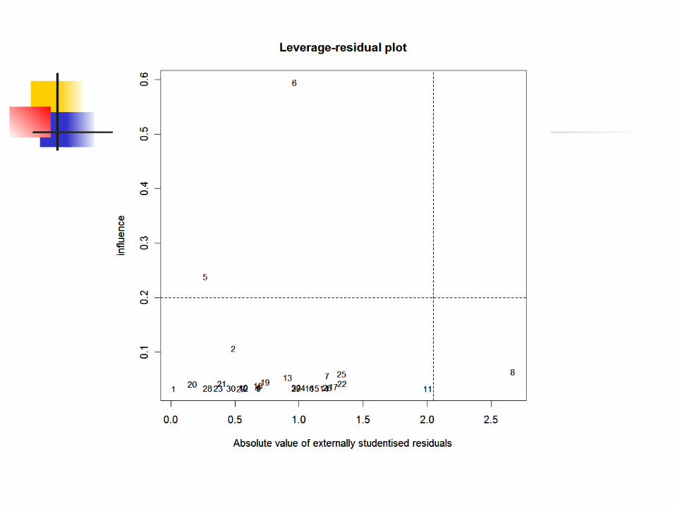
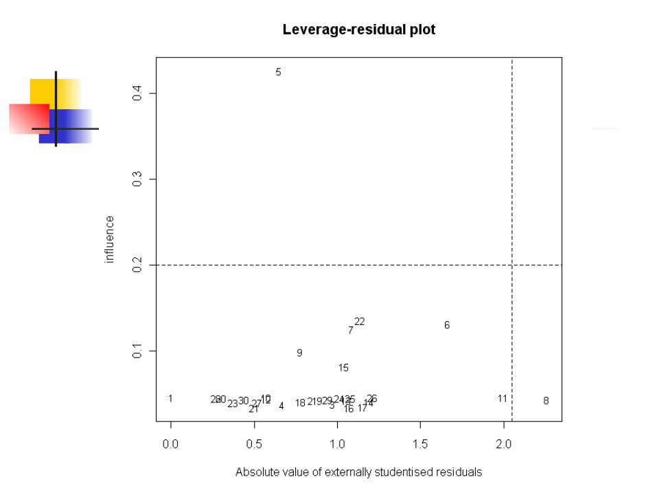
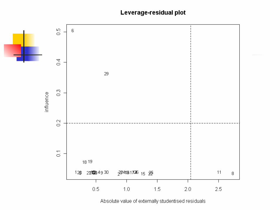
Leverage-residual plot
- Top: Influential data points.
- Bottom: Non-influential data points.
- Left: Non-outliers.
- Right: Outliers.
Upshot: Eliminate points in the top right quadrant as influential outliers.
Life Expectancy
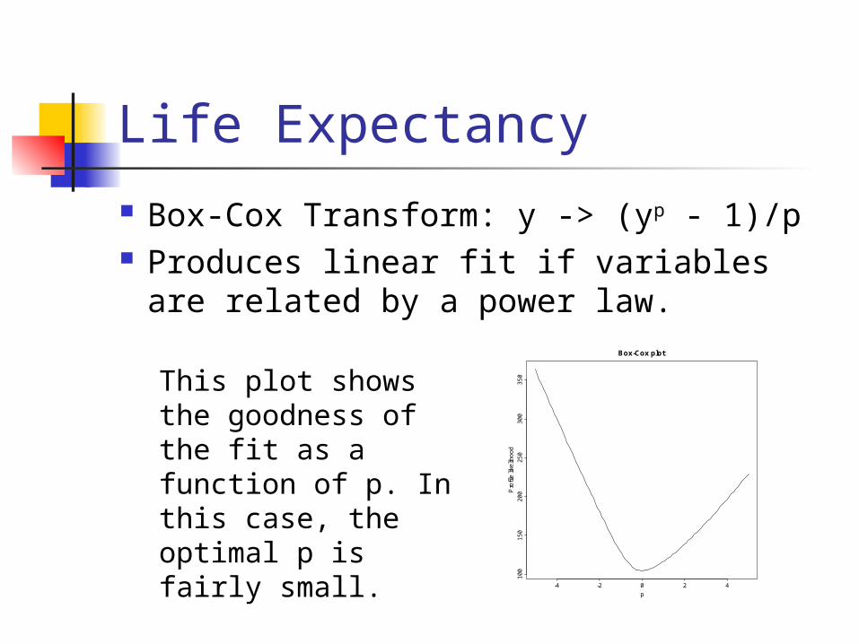
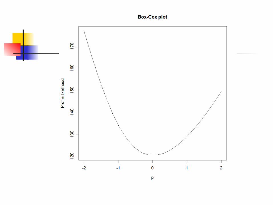
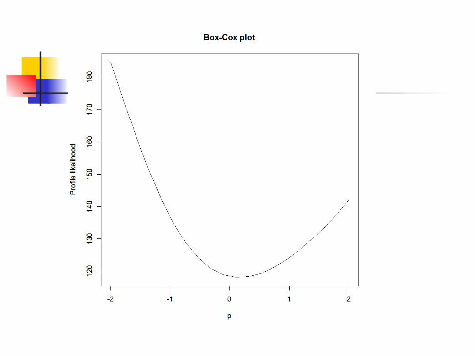
Box-Cox Transform: y -> (yp - 1)/p Produces linear fit if variables are
related by a power law.
-4 -2 0 2 4
10
01
50
20
02
50
30
03
50
Box-Cox plot
p
Pro
file
like
liho
od
This plot shows the goodness of the fit as a function of p. In this case, the optimal p is fairly small.
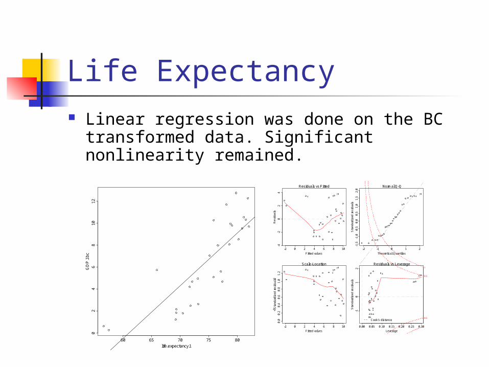
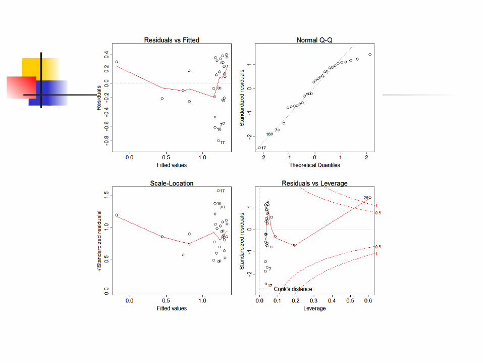
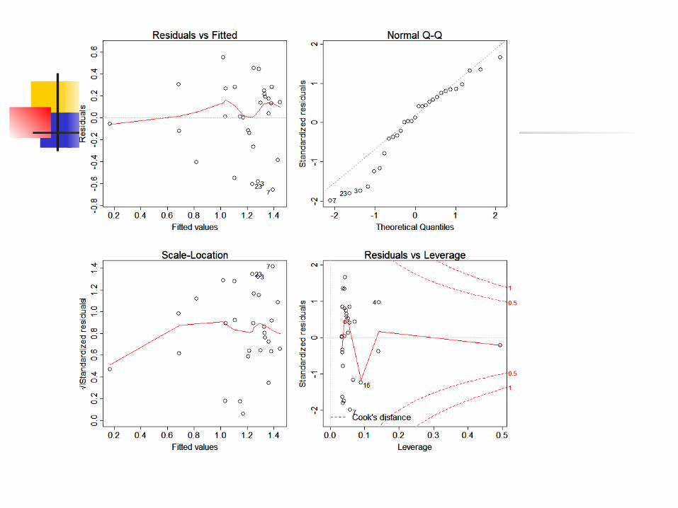
Life Expectancy Linear regression was done on the BC
transformed data. Significant nonlinearity remained.
60 65 70 75 80
02
46
81
01
2
life.expectancy.1
GD
P.1
bc
-2 0 2 4 6 8 10
-4-2
02
4
Fitted values
Res
idua
ls
Residuals vs Fitted
754
-2 -1 0 1 2
-1.5
-1.0
-0.5
0.0
0.5
1.0
1.5
2.0
Theoretical Quantiles
Sta
ndar
dize
d re
sidu
als
Normal Q-Q
745
-2 0 2 4 6 8 10
0.0
0.2
0.4
0.6
0.8
1.0
1.2
Fitted values
Sta
ndar
dize
d re
sidu
als
Scale-Location7
4 5
0.00 0.05 0.10 0.15 0.20 0.25 0.30
-10
12
Leverage
Sta
ndar
dize
d re
sidu
als
Cook's distance0.5
0.5
1
Residuals vs Leverage
13
25
4
Life Expectancy
Conclusions: Clearly, there is a significant positive relationship between per capita GDP and life expectancy.
We could not identify the precise nature of the relationship.
This prevents extrapolation and prediction.
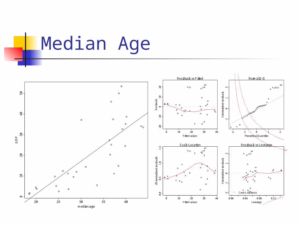
Median Age
20 25 30 35 40
01
02
03
04
05
0
median.age
GD
P
0 10 20 30 40
-20
-10
010
20
Fitted values
Res
idua
ls
Residuals vs Fitted
825 11
-2 -1 0 1 2
-10
12
Theoretical Quantiles
Sta
ndar
dize
d re
sidu
als
Normal Q-Q
8
2511
0 10 20 30 40
0.0
0.5
1.0
1.5
Fitted values
Sta
ndar
dize
d re
sidu
als
Scale-Location8
25 11
0.00 0.04 0.08 0.12
-2-1
01
2
Leverage
Sta
ndar
dize
d re
sidu
als
Cook's distance
0.5
Residuals vs Leverage
8
11
12
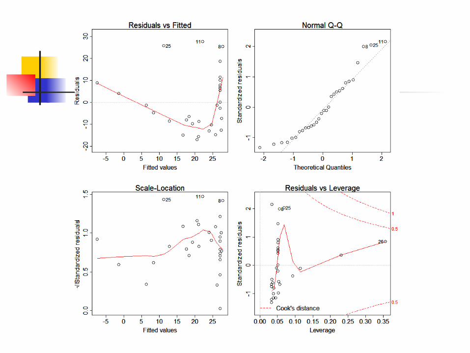
Median Age
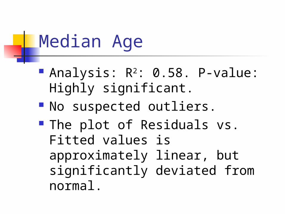
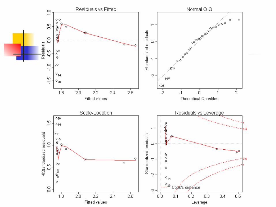
Analysis: R2: 0.58. P-value: Highly significant.
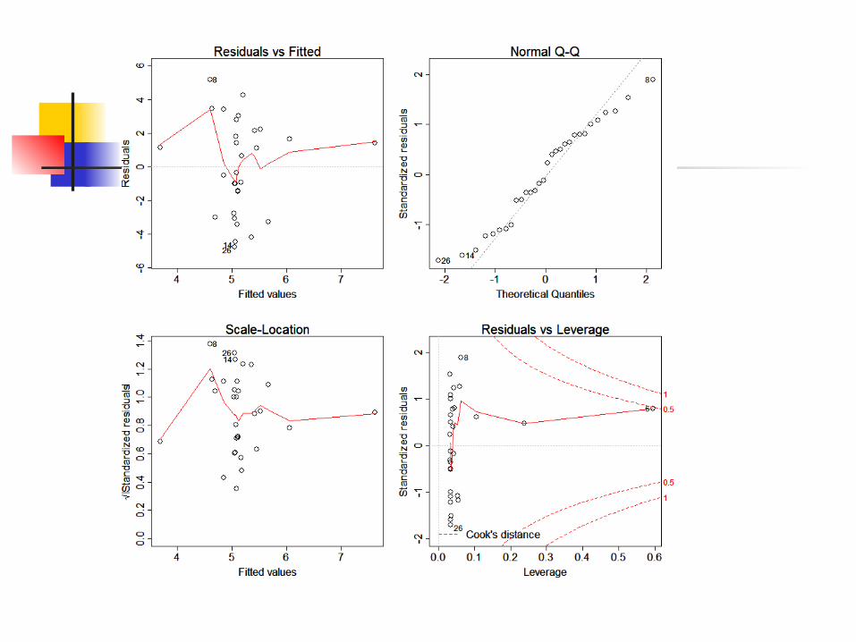
No suspected outliers. The plot of Residuals vs. Fitted
values is approximately linear, but significantly deviated from normal.
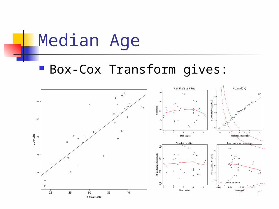
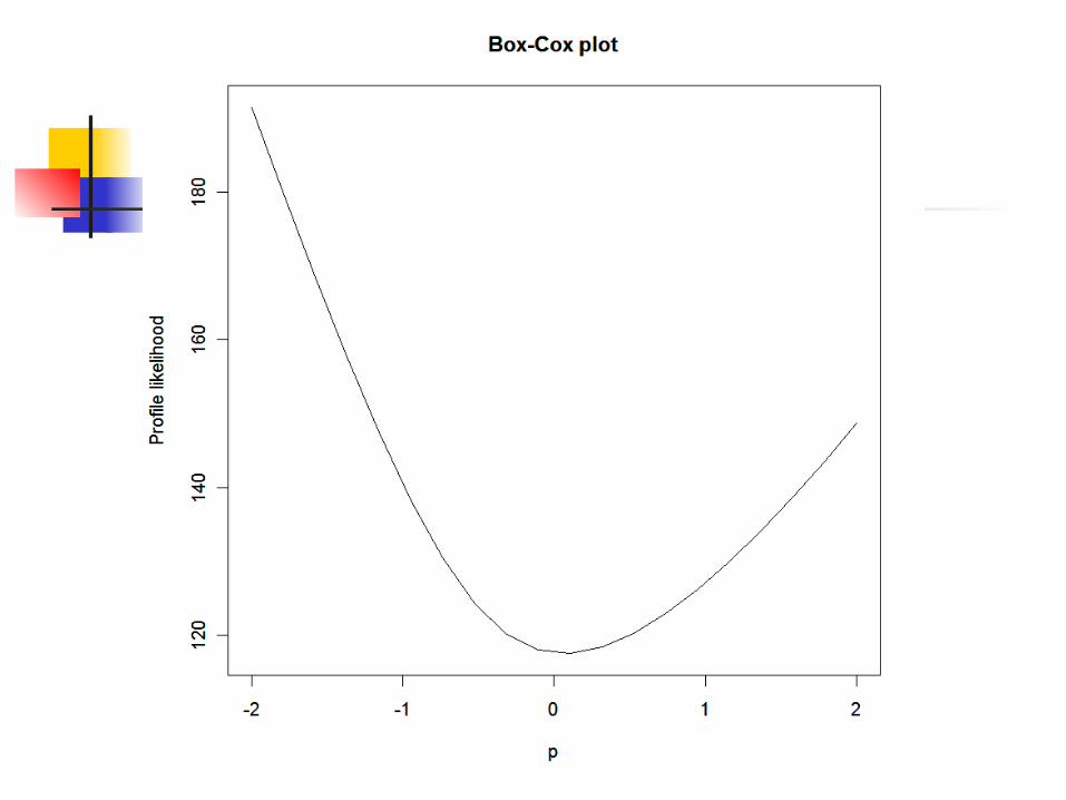
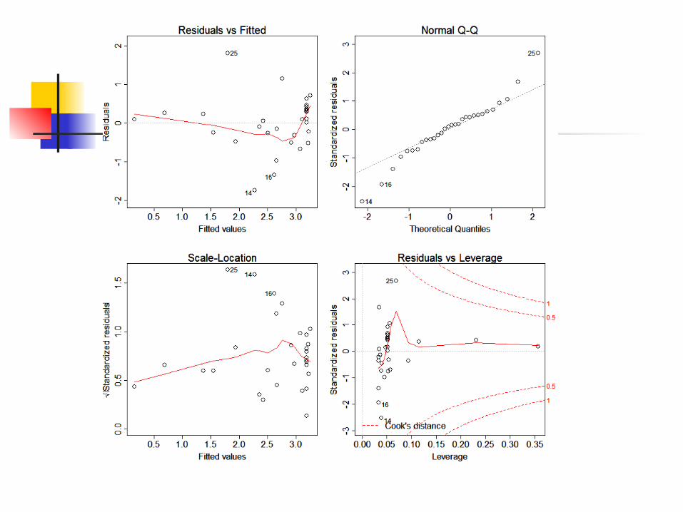
Median Age Box-Cox Transform gives:
20 25 30 35 40
12
34
5
median.age
GD
P.2
bc
1 2 3 4 5
-2-1
01
2
Fitted values
Res
idua
ls
Residuals vs Fitted
25
7
12
-2 -1 0 1 2
-2-1
01
2
Theoretical Quantiles
Sta
ndar
dize
d re
sidu
als
Normal Q-Q
25
7
12
1 2 3 4 5
0.0
0.5
1.0
1.5
Fitted values
Sta
ndar
dize
d re
sidu
als
Scale-Location25
7
12
0.00 0.04 0.08 0.12
-2-1
01
2
Leverage
Sta
ndar
dize
d re
sidu
als
Cook's distance 0.5
0.5
Residuals vs Leverage
25
26
7
Median Age
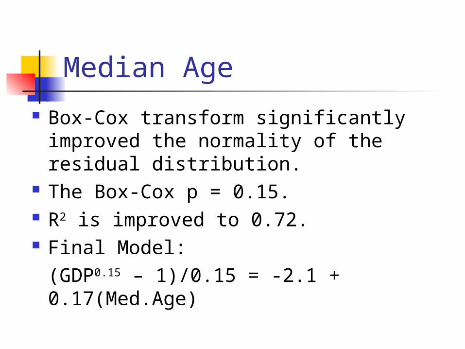
Box-Cox transform significantly improved the normality of the residual distribution.
The Box-Cox p = 0.15. R2 is improved to 0.72. Final Model:
(GDP0.15 – 1)/0.15 = -2.1 + 0.17(Med.Age)
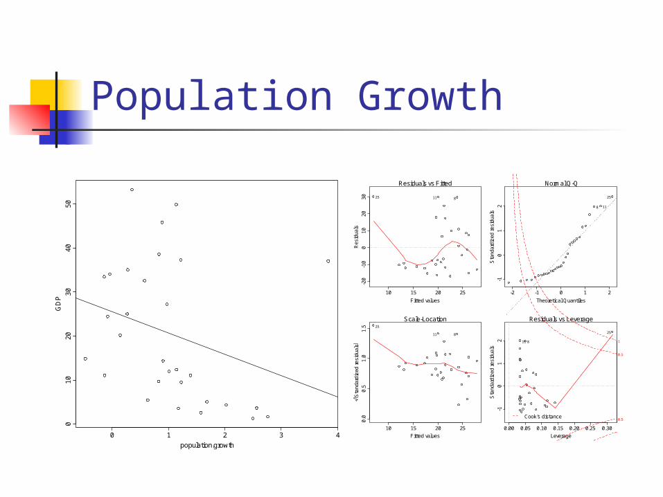
Population Growth
0 1 2 3 4
01
02
03
04
05
0
population.growth
GD
P
10 15 20 25
-20
-10
010
2030
Fitted values
Res
idua
ls
Residuals vs Fitted
25 11 8
-2 -1 0 1 2
-10
12
Theoretical Quantiles
Sta
ndar
dize
d re
sidu
als
Normal Q-Q
25
118
10 15 20 25
0.0
0.5
1.0
1.5
Fitted values
Sta
ndar
dize
d re
sidu
als
Scale-Location25
11 8
0.00 0.05 0.10 0.15 0.20 0.25 0.30
-10
12
Leverage
Sta
ndar
dize
d re
sidu
als
Cook's distance0.5
0.5
1
Residuals vs Leverage
25
811
Population Growth
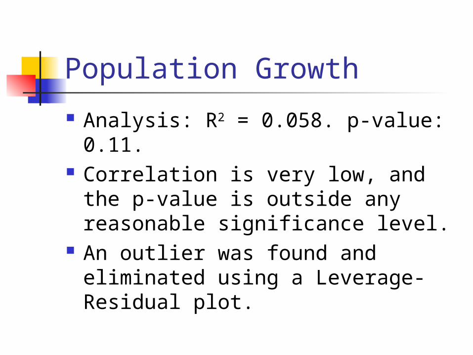
Analysis: R2 = 0.058. p-value: 0.11. Correlation is very low, and the p-
value is outside any reasonable significance level.
An outlier was found and eliminated using a Leverage-Residual plot.
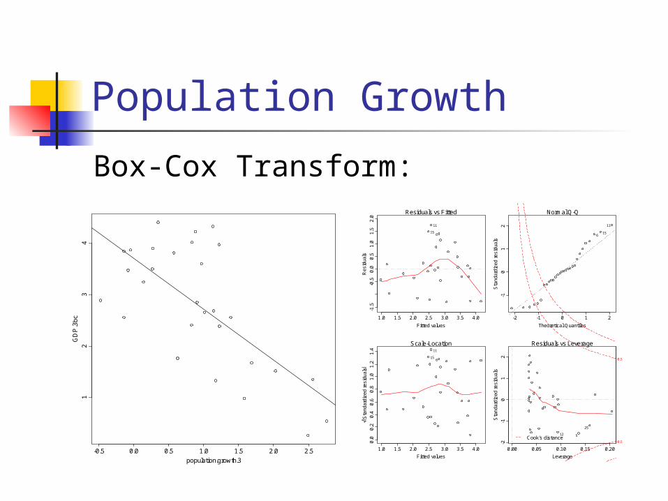
Population Growth
Box-Cox Transform:
-0.5 0.0 0.5 1.0 1.5 2.0 2.5
12
34
population.growth.3
GD
P.3
bc 1.0 1.5 2.0 2.5 3.0 3.5 4.0
-1.5
-0.5
0.0
0.5
1.0
1.5
2.0
Fitted values
Res
idua
ls
Residuals vs Fitted
11
156
-2 -1 0 1 2
-10
12
Theoretical Quantiles
Sta
ndar
dize
d re
sidu
als
Normal Q-Q
11
156
1.0 1.5 2.0 2.5 3.0 3.5 4.0
0.0
0.2
0.4
0.6
0.8
1.0
1.2
1.4
Fitted values
Sta
ndar
dize
d re
sidu
als
Scale-Location11
156
0.00 0.05 0.10 0.15 0.20
-2-1
01
2
Leverage
Sta
ndar
dize
d re
sidu
als
Cook's distance0.5
0.5
Residuals vs Leverage
5
25
12
Population Growth
A Box-Cox transform improved the nonlinearity slightly, and gave a significant p-value.
From this, we concluded that population growth has a slight negative relationship with GDP.
No detailed predictions are possible because significant nonlinearity remains.
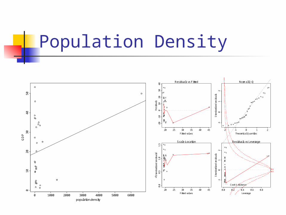
Population Density
0 1000 2000 3000 4000 5000 6000
01
02
03
04
05
0
population.density
GD
P
20 25 30 35 40 45
-20
-10
010
2030
40
Fitted values
Res
idua
ls
Residuals vs Fitted
8
6
22
-2 -1 0 1 2
-10
12
Theoretical Quantiles
Sta
ndar
dize
d re
sidu
als
Normal Q-Q
8
6
11
20 25 30 35 40 45
0.0
0.5
1.0
1.5
Fitted values
Sta
ndar
dize
d re
sidu
als
Scale-Location8
6
11
0.0 0.2 0.4 0.6 0.8
-10
12
Leverage
Sta
ndar
dize
d re
sidu
als
Cook's distance
10.50.51
Residuals vs Leverage
11
8
6
Population Density
Analysis: The outlier on the far right corresponds to Singapore, a country with an exceptionally high population density.
A less extreme outlier is China. Both of these data points were removed.
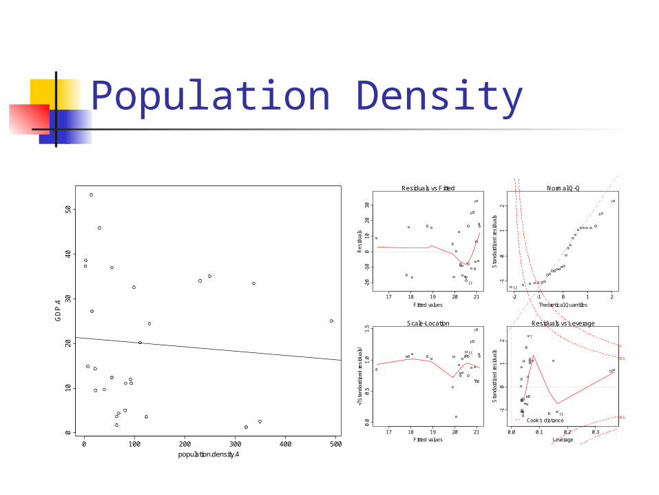
Population Density
0 100 200 300 400 500
01
02
03
04
05
0
population.density.4
GD
P.4
17 18 19 20 21
-20
-10
010
2030
Fitted values
Res
idua
ls
Residuals vs Fitted
7
6
12
-2 -1 0 1 2
-10
12
Theoretical Quantiles
Sta
ndar
dize
d re
sidu
als
Normal Q-Q
7
6
12
17 18 19 20 21
0.0
0.5
1.0
1.5
Fitted values
Sta
ndar
dize
d re
sidu
als
Scale-Location7
6
12
0.0 0.1 0.2 0.3
-10
12
Leverage
Sta
ndar
dize
d re
sidu
als
Cook's distance0.5
0.5
1
Residuals vs Leverage
7
18
15
Population Density
The p-value for the data without outliers is a very insignificant 0.68.
A Box-Cox transform was attempted, but the p-value did not get close to significance.
Conclusion: Population density and GDP are essentially unrelated.
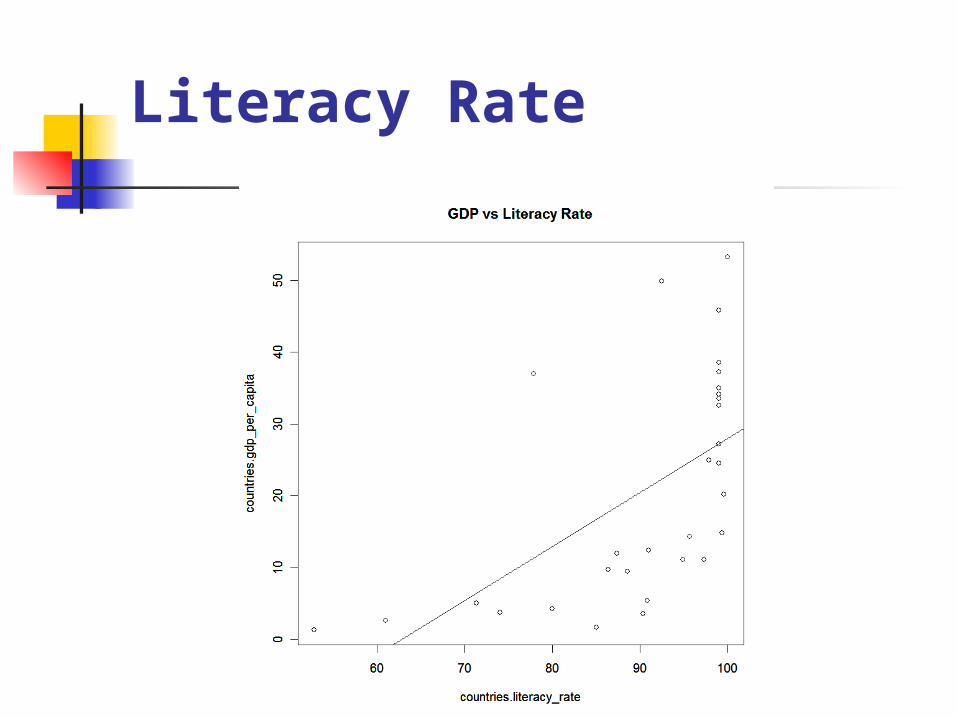
Literacy Rate

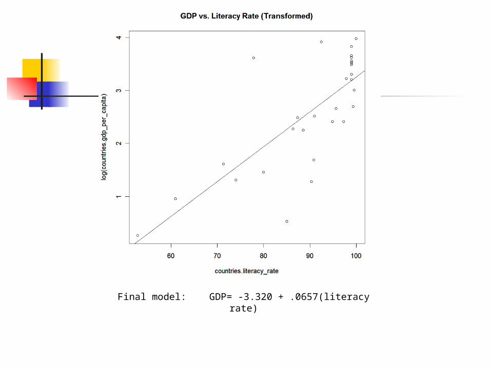
Final model: GDP= -3.320 + .0657(literacy rate)
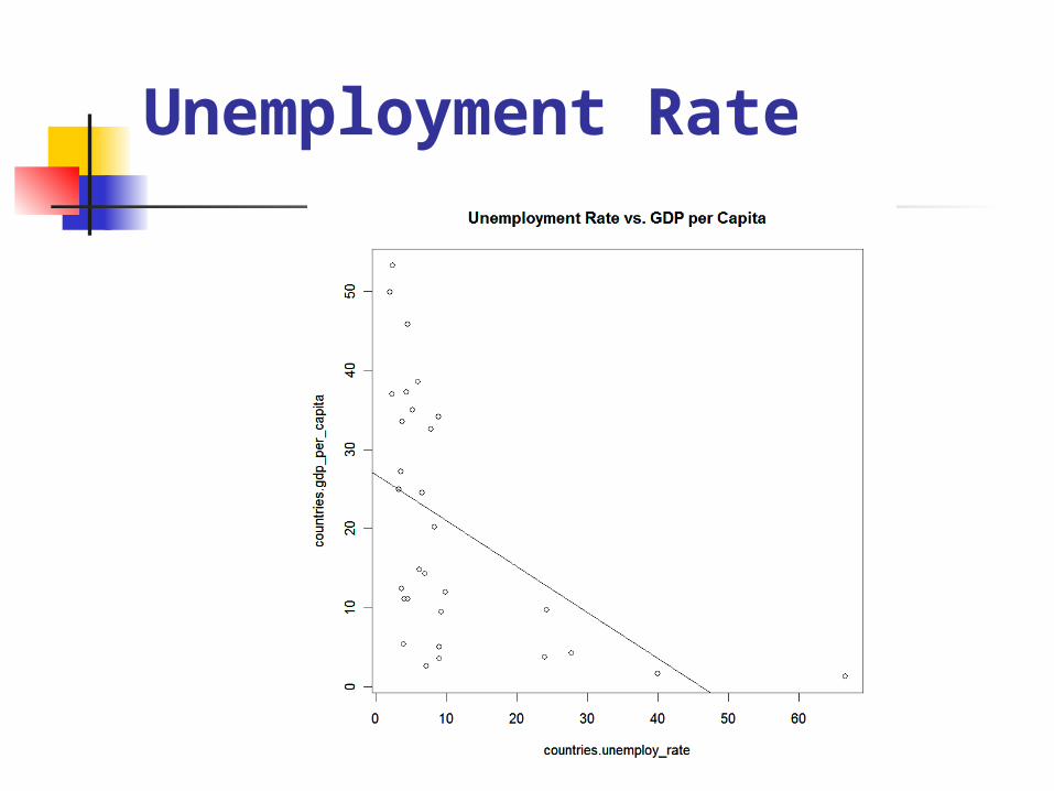
Unemployment Rate
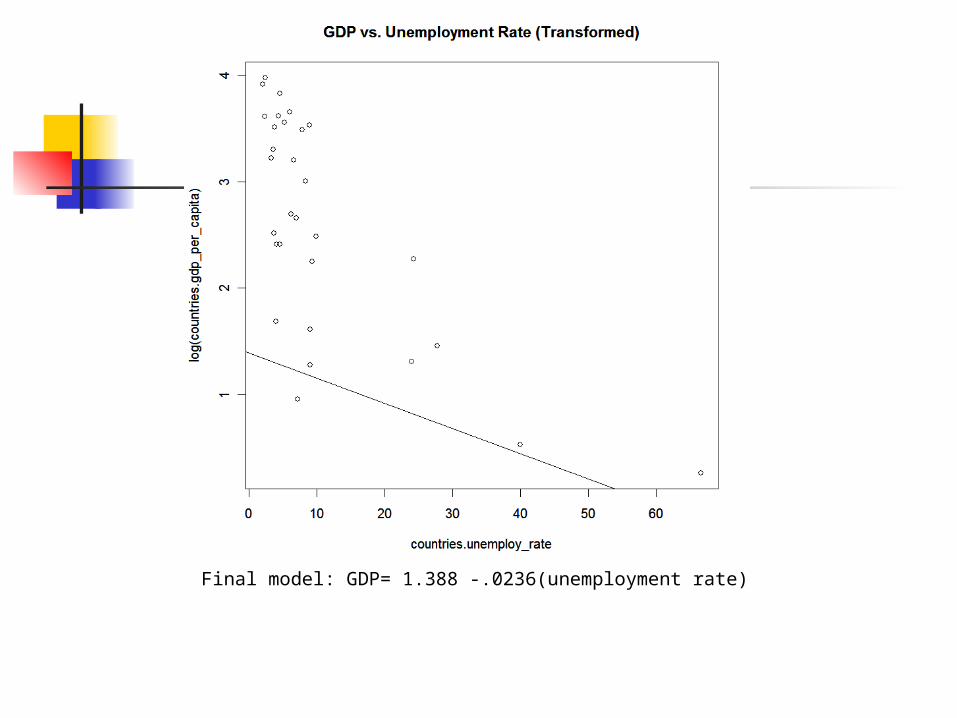
Final model: GDP= 1.388 -.0236(unemployment rate)

Oil Consumption – Production

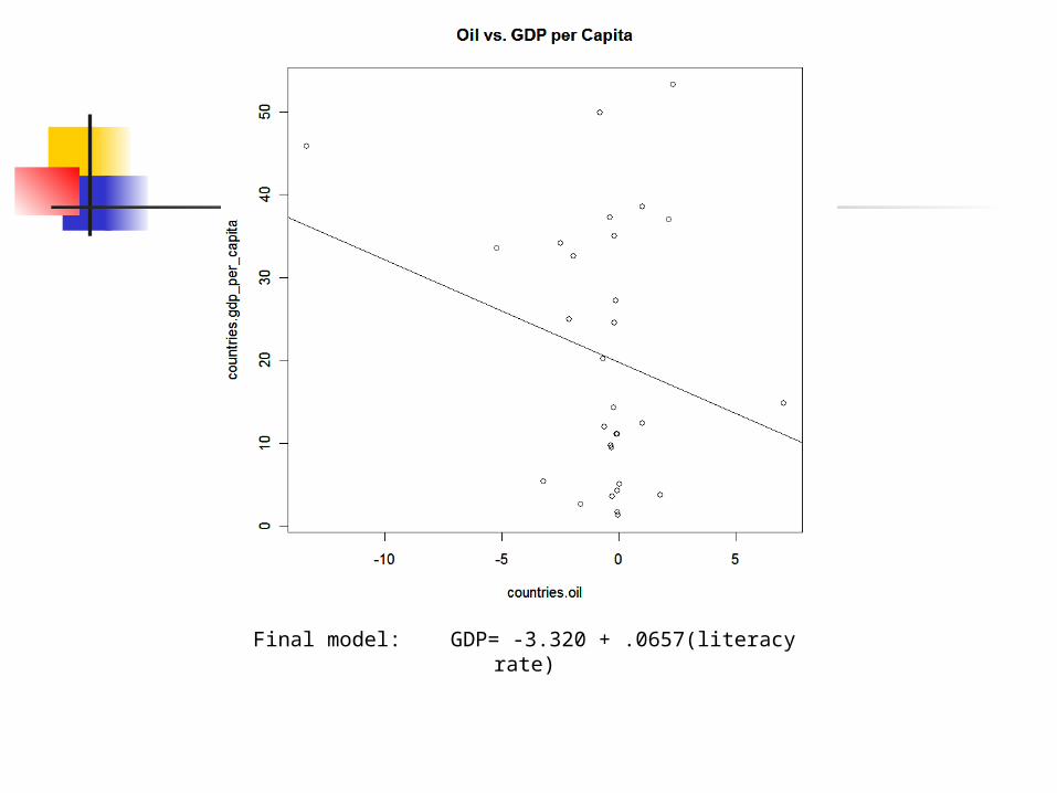
Final model: GDP= -3.320 + .0657(literacy rate)
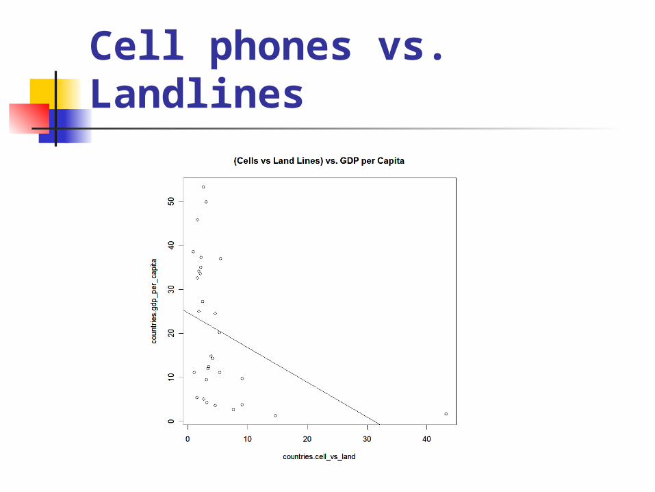
Cell phones vs. Landlines
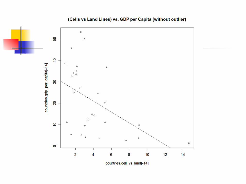
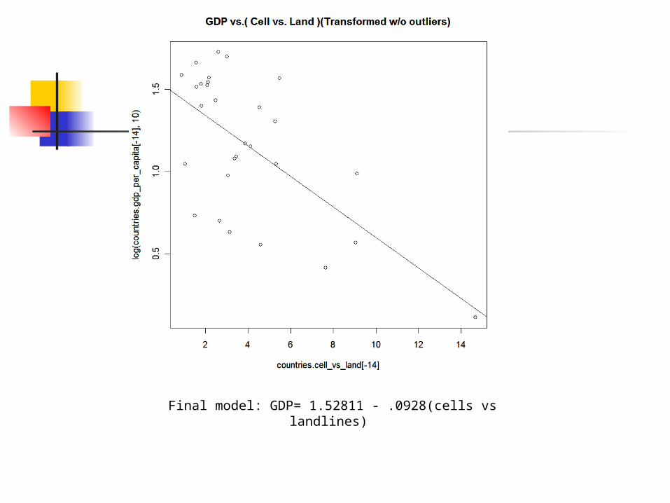
Final model: GDP= 1.52811 - .0928(cells vs landlines)
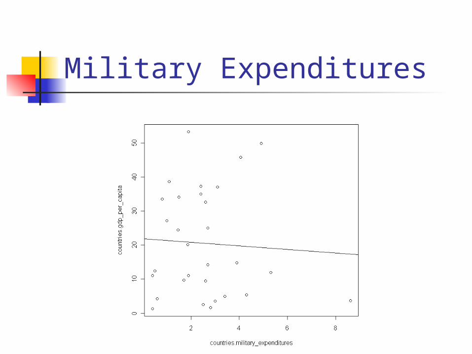
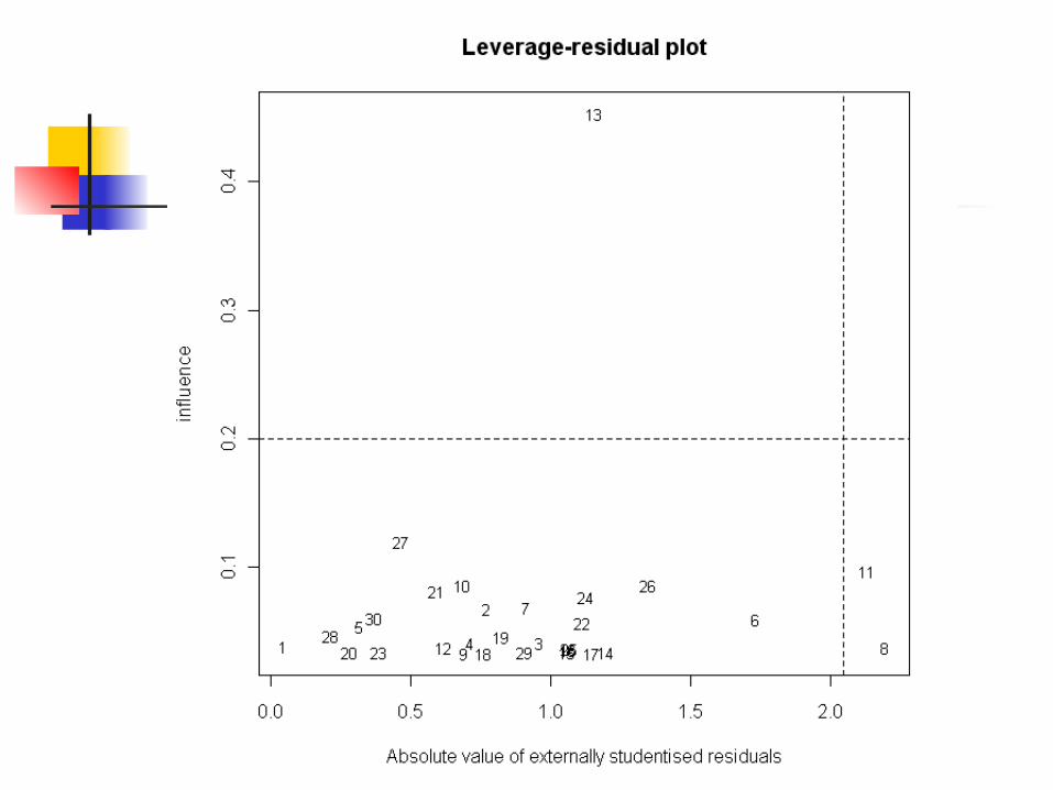
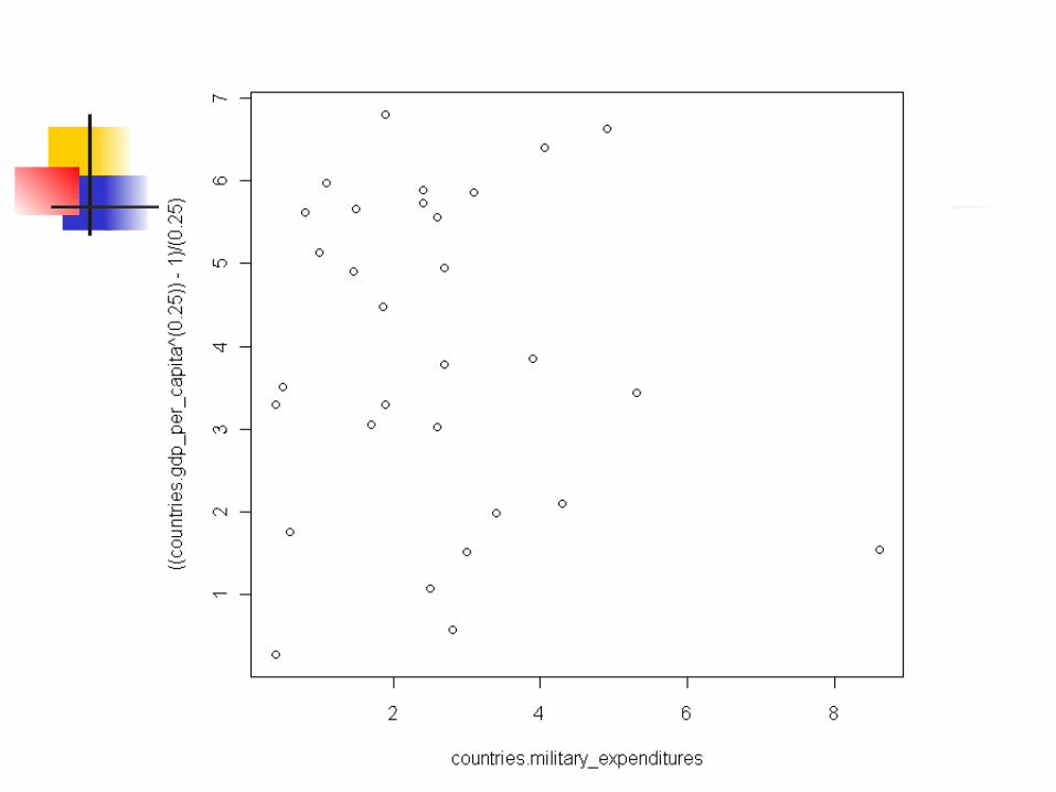
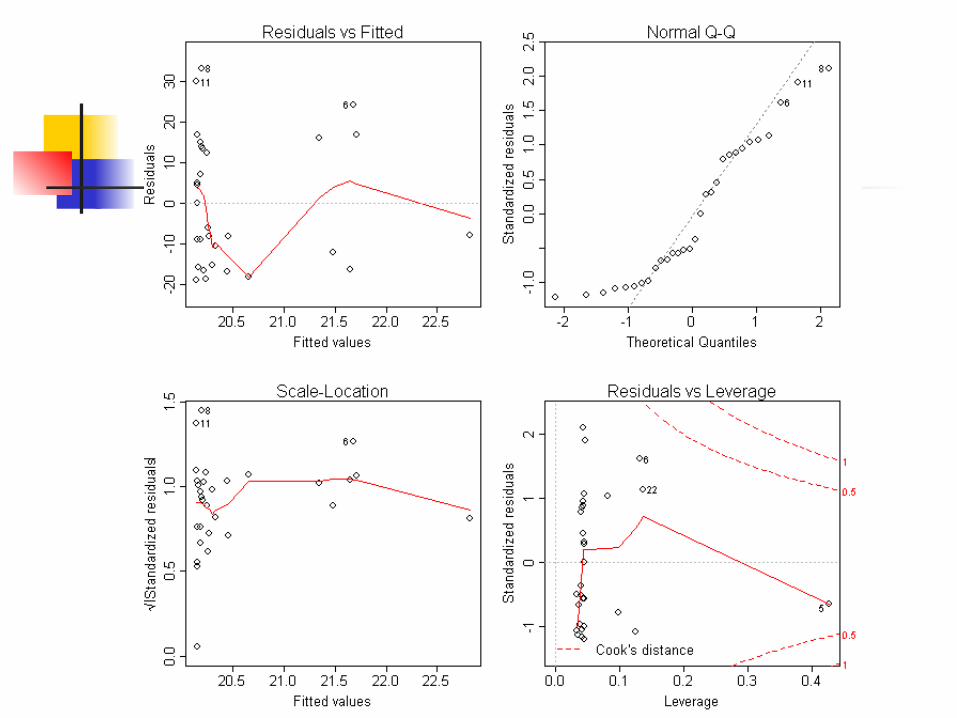
Military Expenditures
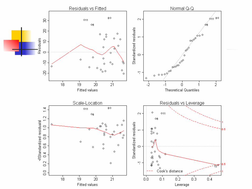

Analysis
Doesn’t pass conditions for regression Data isn’t linear Residuals aren’t random Q-Q plot is curved Outliers
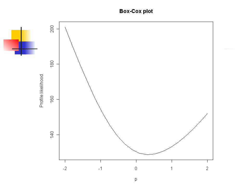
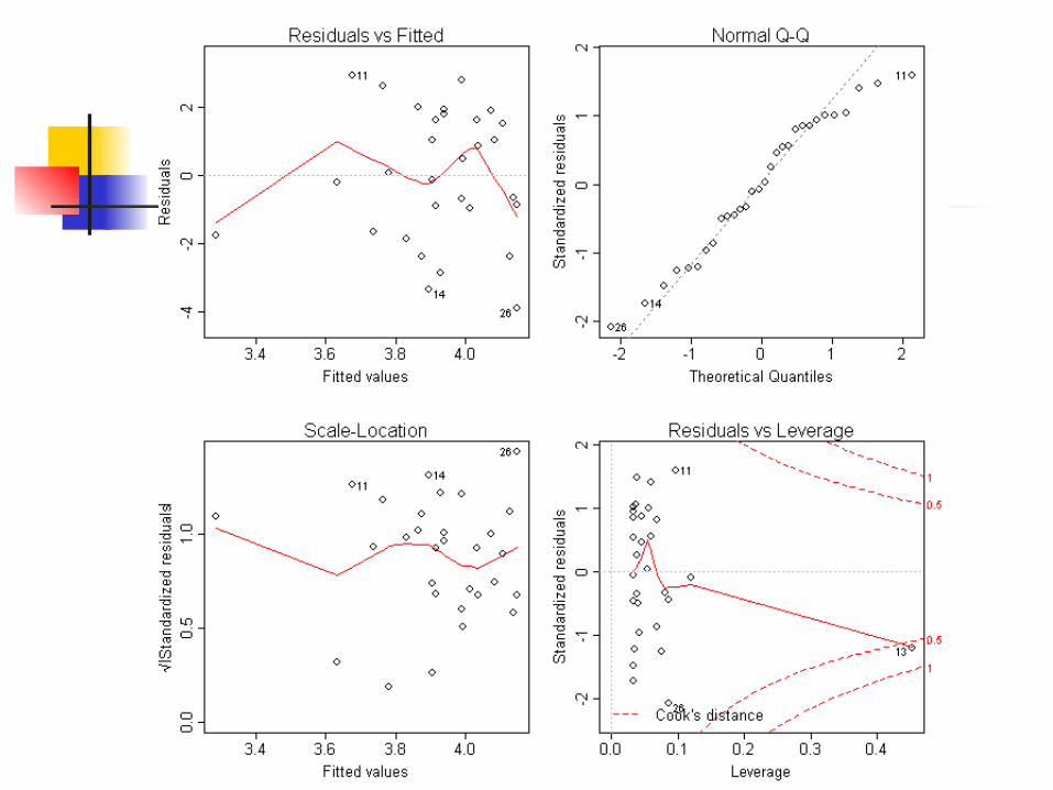
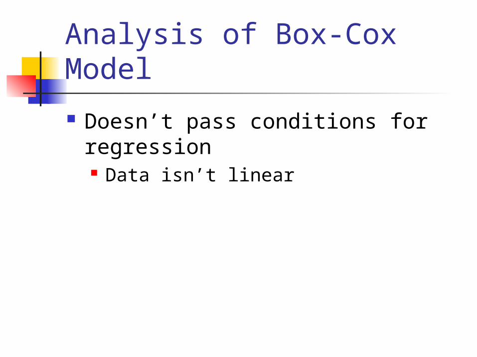
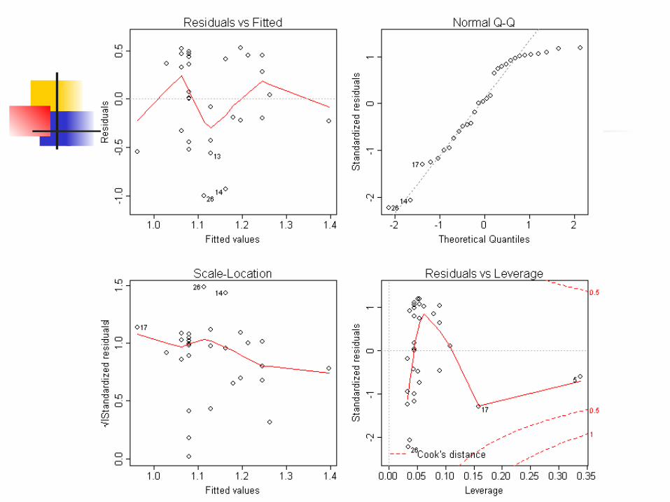
Analysis of Box-Cox Model
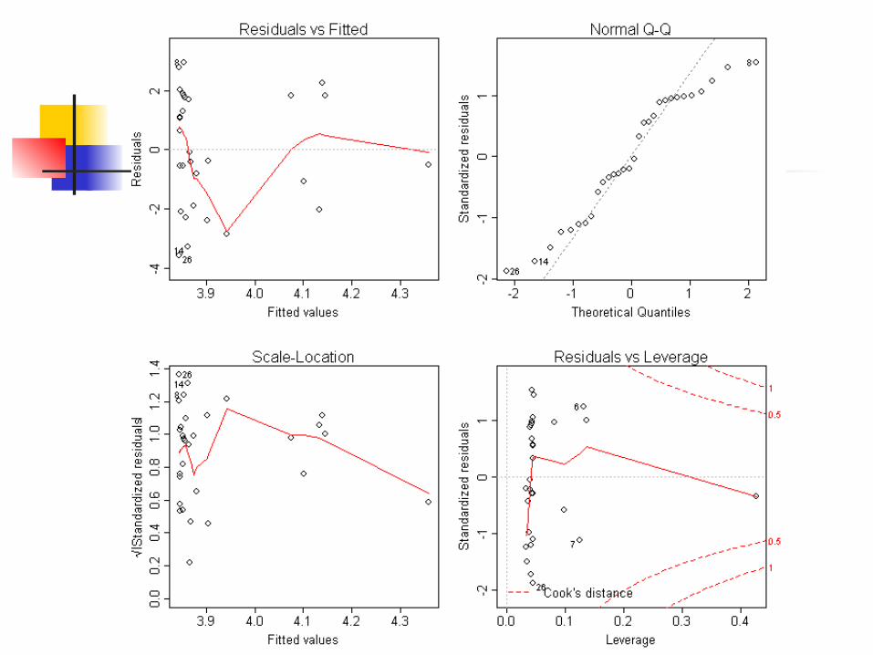
Doesn’t pass conditions for regression Data isn’t linear
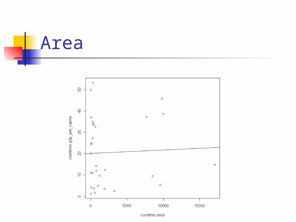
Area
Analysis
Doesn’t pass conditions for regression Data isn’t linear Residuals aren’t random Q-Q plot is curved Outliers


Analysis of Box-Cox Model
Doesn’t pass conditions for regression Data isn’t linear Residuals are not random Q-Q plot isn’t normal
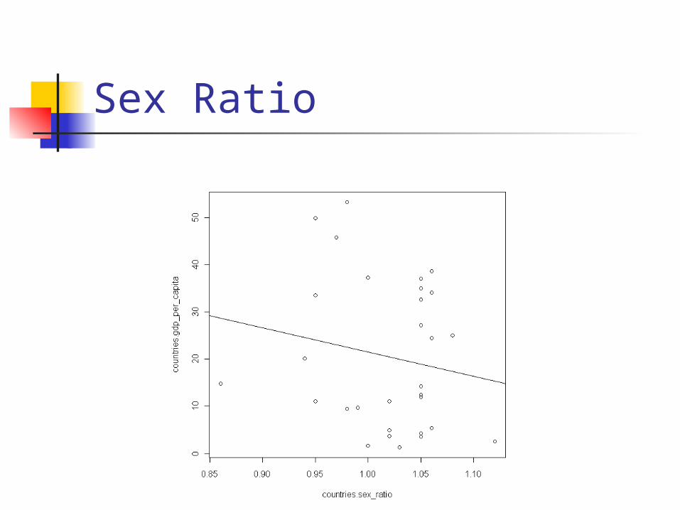
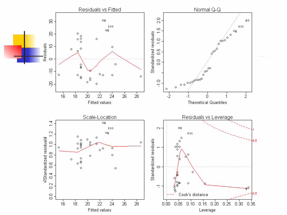
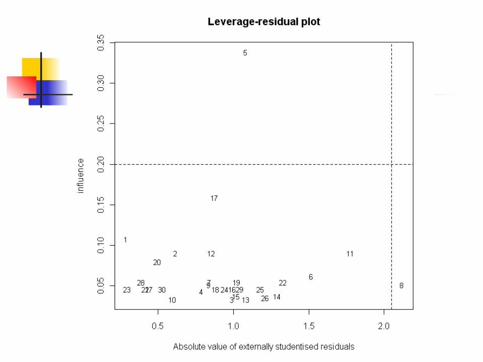
Sex Ratio

Analysis
Doesn’t pass conditions for regression Data isn’t linear Residuals aren’t random Q-Q plot is curved Outliers
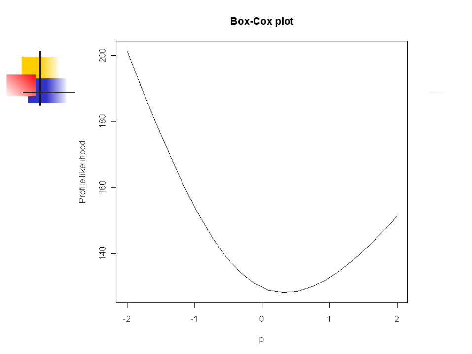
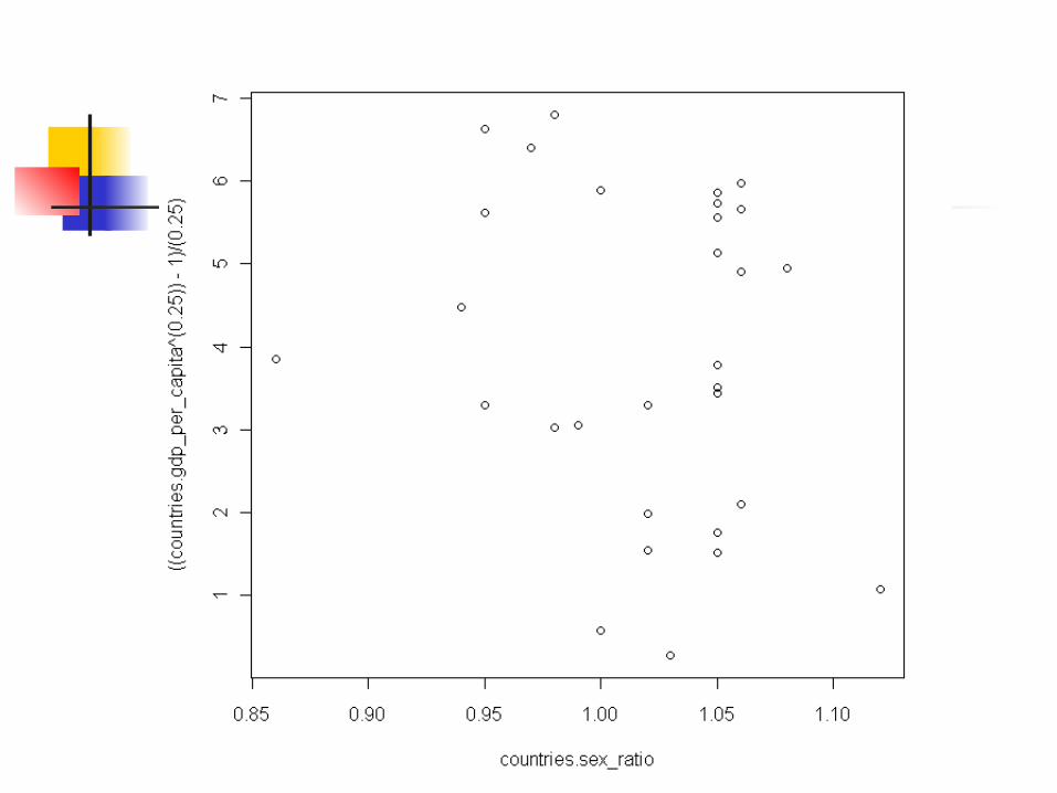
Analysis of Box-Cox Model
Doesn’t pass conditions for regression Data isn’t linear Residuals are not random Q-Q plot isn’t normal
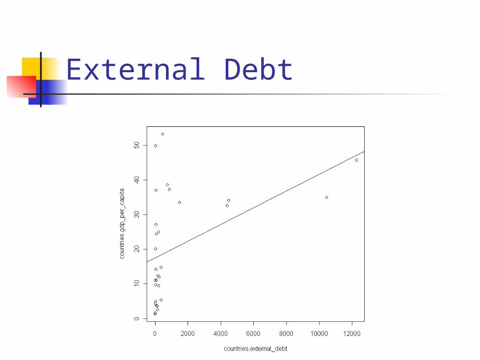
External Debt

Analysis
Doesn’t pass conditions for regression Data isn’t linear Residuals aren’t random Q-Q plot is curved Outliers


Analysis of Box-Cox Model
Doesn’t pass conditions for regression Data isn’t linear Residuals are not random Q-Q plot isn’t normal
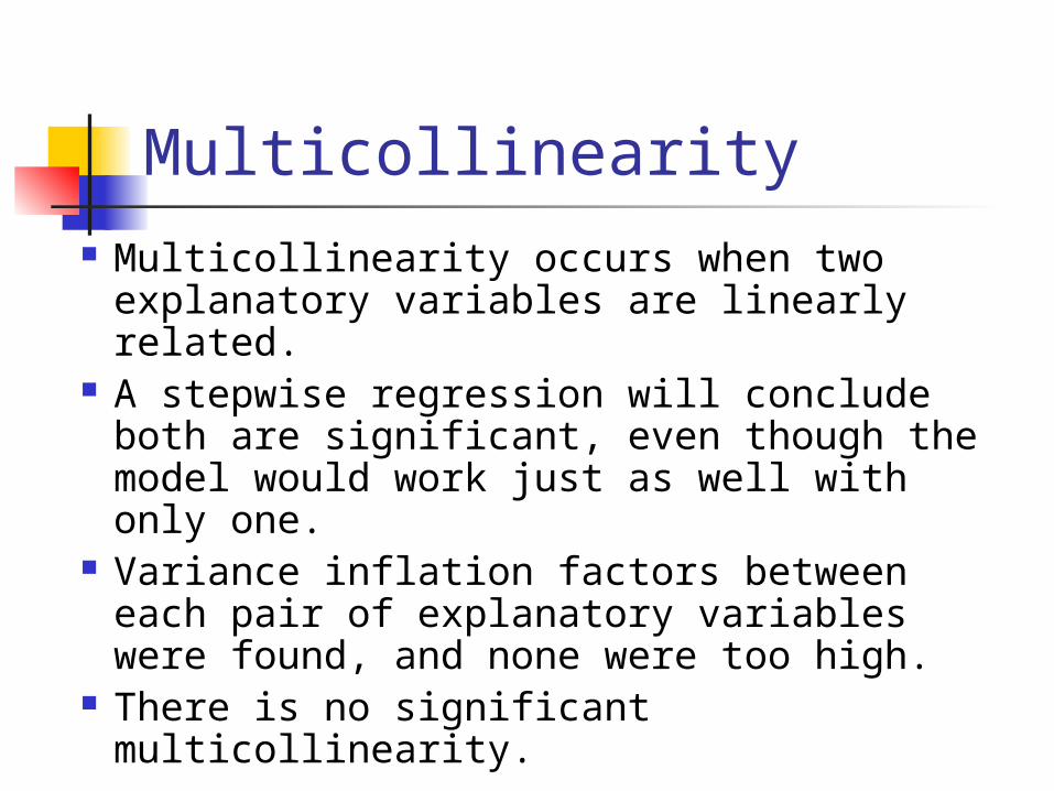
Multicollinearity Multicollinearity occurs when two
explanatory variables are linearly related. A stepwise regression will conclude both
are significant, even though the model would work just as well with only one.
Variance inflation factors between each pair of explanatory variables were found, and none were too high.
There is no significant multicollinearity.
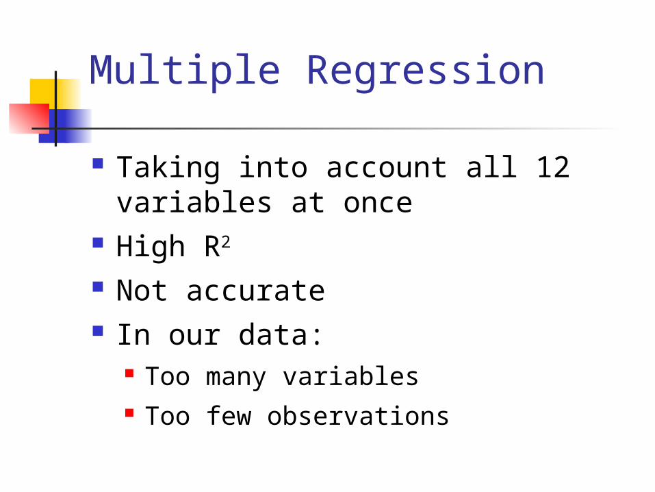
Multiple Regression
Taking into account all 12 variables at once
High R2
Not accurate In our data:
Too many variables Too few observations
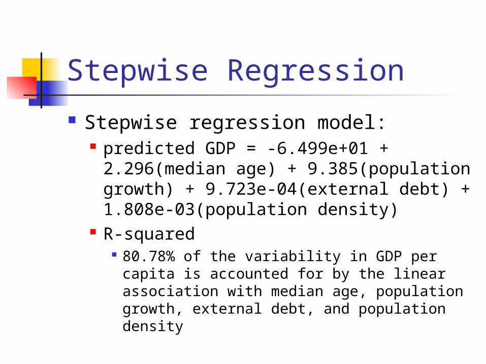
Stepwise Regression
Stepwise regression model: predicted GDP = -6.499e+01 +
2.296(median age) + 9.385(population growth) + 9.723e-04(external debt) + 1.808e-03(population density)
R-squared 80.78% of the variability in GDP per capita
is accounted for by the linear association with median age, population growth, external debt, and population density
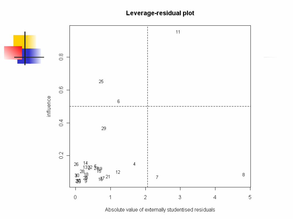
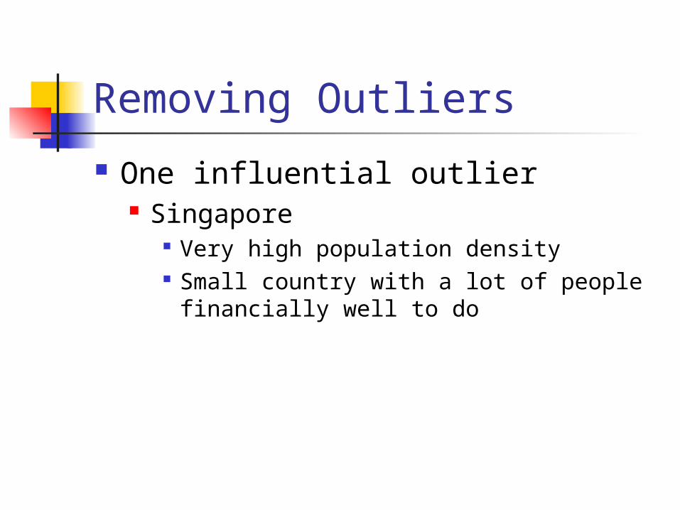
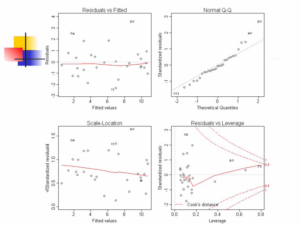
Removing Outliers
One influential outlier Singapore
Very high population density Small country with a lot of people
financially well to do
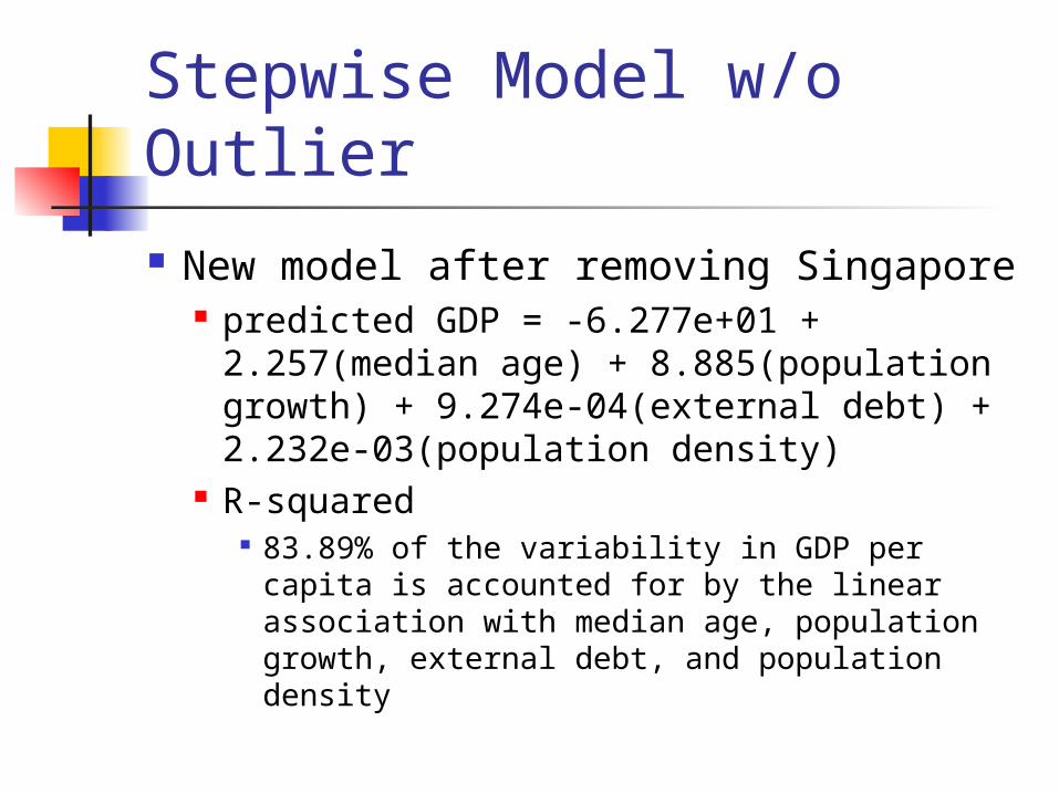
Stepwise Model w/o Outlier
New model after removing Singapore predicted GDP = -6.277e+01 +
2.257(median age) + 8.885(population growth) + 9.274e-04(external debt) + 2.232e-03(population density)
R-squared 83.89% of the variability in GDP per capita
is accounted for by the linear association with median age, population growth, external debt, and population density

Box-Cox Transformation
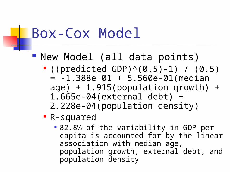
Box-Cox Model New Model (all data points)
((predicted GDP)^(0.5)-1) / (0.5) = -1.388e+01 + 5.560e-01(median age) + 1.915(population growth) + 1.665e-04(external debt) + 2.228e-04(population density)
R-squared 82.8% of the variability in GDP per capita
is accounted for by the linear association with median age, population growth, external debt, and population density
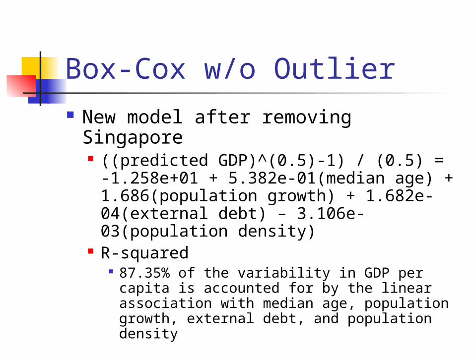
Box-Cox w/o Outlier New model after removing Singapore
((predicted GDP)^(0.5)-1) / (0.5) = -1.258e+01 + 5.382e-01(median age) + 1.686(population growth) + 1.682e-04(external debt) – 3.106e-03(population density)
R-squared 87.35% of the variability in GDP per capita is
accounted for by the linear association with median age, population growth, external debt, and population density
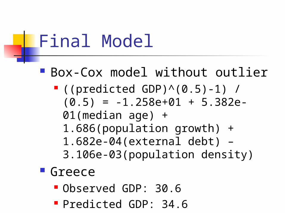
Final Model
Box-Cox model without outlier ((predicted GDP)^(0.5)-1) / (0.5) = -
1.258e+01 + 5.382e-01(median age) + 1.686(population growth) + 1.682e-04(external debt) – 3.106e-03(population density)
Greece Observed GDP: 30.6 Predicted GDP: 34.6