THE TOPOLOGY OF TORIC ORIGAMI MANIFOLDS

TARA S. HOLM AND ANA RITA PIRES

ABSTRACT. A folded symplectic form on a manifold is a closed 2-form with the mildest possible de-generacy along a hypersurface. A special class of folded symplectic manifolds are the origami sym-plectic manifolds, studied by Cannas da Silva, Guillemin and Pires, who classified toric origami man-ifolds by combinatorial origami templates. In this paper, we examine the topology of toric origamimanifolds that have acyclic origami template and coorientable folding hypersurface. We prove thatthe cohomology is concentrated in even degrees, and that the equivariant cohomology satisfies theGKM description. Finally we show that toric origami manifolds with coorientable folding hypersur-face provide a class of examples of Masuda and Panov’s torus manifolds.

CONTENTS

1. Introduction 12. Origami manifolds 23. Cohomology concentrated in even degrees 64. Equivariant cohomology 115. Toric origami manifolds are locally standard 16References 18

1. INTRODUCTION

Toric symplectic manifolds are a useful class of examples for testing general theories and mak-ing explicit computations. Statements and proofs of important theorems often simplify in the caseof toric manifolds. Delzant’s classification of toric symplectic manifolds in terms of convex poly-topes allows the translation of geometric and topological questions into combinatorial ones. Inthis paper, we study toric actions in the category of folded symplectic manifolds. Relaxing therequirement that the manifold be symplectic broadens the class of manifolds with toric actions.The mildest degeneracy is to allow the 2-form to be zero along a hypersurface. In this instance,there remains enough geometric structure to be able to classify such toric origami manifolds com-binatorially.

In this paper, we study the topology of a particular class of toric origami manifolds, those withacyclic template and coorientable fold. For such manifolds, we prove that the ordinary cohomol-ogy is concentrated in even degrees (Theorem 3.6). This allows us to deduce a variety of factsabout the equivariant cohomology of these manifolds, and in particular to describe the equivari-ant cohomology ring combinatorially (Theorem 4.12). Our class of toric origami manifolds does fitinto the framework of torus manifolds (Theorem 5.3). The origami structure allows us to give ex-plicit inductive proofs. We plan to use similar geometric techniques to study the non-coorientableand non-acyclic cases. We hope that this approach will also generalize to a class of torus manifolds

Date: November 15, 2013.2010 Mathematics Subject Classification. Primary: 53D20; Secondary: 55N91, 57R91.Tara Holm was partially supported by Grant #208975 from the Simons Foundation and NSF Grant DMS–1206466.Ana Rita Pires was partially supported by an AMS-Simons Travel Grant.

1

arX

iv:1

211.

6435

v3 [

mat

h.SG

] 1

4 N

ov 2

013

that arise from combinatorial origami templates, in the same way that some torus manifolds arisefrom combinatorial polytopes.

The remainder of this paper is organized as follows. In Section 2, we review the symplectic andfolded symplectic geometry underlying our work. We then provide a framework for computingthe ordinary and equivariant cohomology of origami manifolds with coorientable folding hyper-surface and acyclic template in Sections 3 and 4. In Section 5 we describe the relationship of ourwork with the toric topology literature.Acknowledgements. We are grateful to Jean-Claude Hausmann for his help and patience whenwe were sorting out the commutativity of diagram (3.12); and to Nick Sheridan for his suggestionsregarding Definition 2.8. We would also like to thank Ana Cannas da Silva, Victor Guillemin, AllenHatcher, Yael Karshon, Allen Knutson, Tomoo Matsumura, and Milena Pabiniak for many helpfulconversations. We are very grateful for the comments from the anonymous referees, which led toseveral improvements of this article.

2. ORIGAMI MANIFOLDS

2.1. Symplectic manifolds. We begin with a very quick review of symplectic geometry, following[C2]. Let M be a manifold equipped with a symplectic form ω ∈ Ω2(M): that is, ω is closed(dω = 0) and non-degenerate. In particular, the non-degeneracy condition implies that M mustbe an even-dimensional manifold. The simplest examples include

(1) M = S2 = CP1 withωp(X,Y) = signed area of the parallelogram spanned by X and Y;(2) M any compact orientable surface withω the area form; and(3) M = R2d with ω =

∑dxi ∧ dyi. The Darboux Theorem says that every symplectic mani-

fold has local coordinates so thatω is of this standard form.Suppose that a compact connected abelian Lie group T = (S1)n acts on M preserving ω. The

action is weakly Hamiltonian if for every vector ξ ∈ t in the Lie algebra t of T, the vector field

Xξ(p) =d

dt

[exp(tξ) · p

]∣∣∣∣t=0

is a Hamiltonian vector field. That is, we requireω(Xξ, ·) to be an exact one-form1:

(2.1) ω(Xξ, ·) = dφξ.

Thus each φξ is a smooth function on M defined by the differential equation (2.1), so determinedup to a constant. Taking them together, we may define a moment map

Φ :M −→ t∗

p 7→ (t −→ Rξ 7→ φξ(p)

).

The action is Hamiltonian if the moment mapΦ can be chosen to be a T-invariant map. Atiyahand Guillemin-Sternberg have shown that when M is a compact Hamiltonian T-manifold, theimageΦ(M) is a convex polytope, and is the convex hull of the images of the fixed pointsΦ(MT)[A, GS].

For an effective2 Hamiltonian T action on M, dim(T) ≤ 12 dim(M). We say that the action is

toric if this inequality is in fact an equality. A symplectic manifold M with a toric HamiltonianT action is called a symplectic toric manifold. Delzant used the moment polytope to classifysymplectic toric manifolds.

1 The one-formω(Xξ, ·) is automatically closed because the action preservesω.2 An action is effective if no non-trivial subgroup acts trivially.

2

A polytope ∆ in Rn is simple if there are n edges incident to each vertex, and it is rational ifeach edge vector has rational slope: it lies in Qn ⊂ Rn. A simple polytope is smooth at a vertexif the n primitive vectors parallel to the edges at the vertex span the lattice Zn ⊆ Rn over Z. Itis smooth if it is smooth at each vertex. A simple rational smooth convex polytope is called aDelzant polytope. We may now state Delzant’s result.

Theorem 2.2 (Delzant [De]). There is a one-to-one correspondencecompact toric

symplectic manifolds

!

Delzant polytopes,

up to equivariant symplectomorphism on the left-hand side and affine equivalence on the right-hand side.

2.2. Origami manifolds. We now relax the non-degeneracy condition on ω, following [CGP]. Afolded symplectic form on a 2n-dimensional manifold M is a 2-form ω ∈ Ω2(M) that is closed(dω = 0), whose top power ωn intersects the zero section transversely on a subset Z and whoserestriction to points in Z has maximal rank. The transversality forces Z to be a codimension 1embedded submanifold ofM. We call Z the folding hypersurface or fold.

The simplest examples of folded symplectic manifolds include the following.

(1) Euclidean space M = R2d has folded symplectic form ω = x1dx1 ∧ dy1 +∑di=2 dxi ∧ dyi.

The Folded Darboux Theorem says that at points in Z = x1 = 0, every folded symplecticmanifold has local coordinates so thatω is of this standard form [Mar, IIIA.4.2.2].

(2) Any even-dimensional sphereM = S2n ⊂ Cn⊕R may be equipped with the formωCn⊕0.The folding hypersurface is the equator Z = S2n−1 ⊂ Cn ⊕ 0.

(3) Any compact surface M can be equipped with a folded symplectic form with Z a union ofcircles. See, for instance, Example 3.19 of [CGP], and use Remark 2.33 of the same papertogether with the classification of closed surfaces. This includes non-orientable surfaces.For example, RP2 can be equipped with a folded symplectic form so that Z is a single circle.

Let i : Z →M be the inclusion of Z as a submanifold ofM. Our assumptions imply that i∗ω hasa 1-dimensional kernel on Z. This line field is called the null foliation on Z. An origami manifoldis a folded symplectic manifold (M,ω) whose null foliation is fibrating: Z π−→ B is a fiber bundlewith orientable circle fibers over a compact base B. The form ω is called an origami form and thebundle π is called the null fibration. A diffeomorphism between two origami manifolds whichintertwines the origami forms is called an origami-symplectomorphism. In the examples above,the first is not origami because the fibers are R rather than S1, but the second and third are origami.In the second example, the null fibration is the Hopf bundle S2n−1 −→ CPn−1, and in the thirdexample, the base B consists of isolated points.

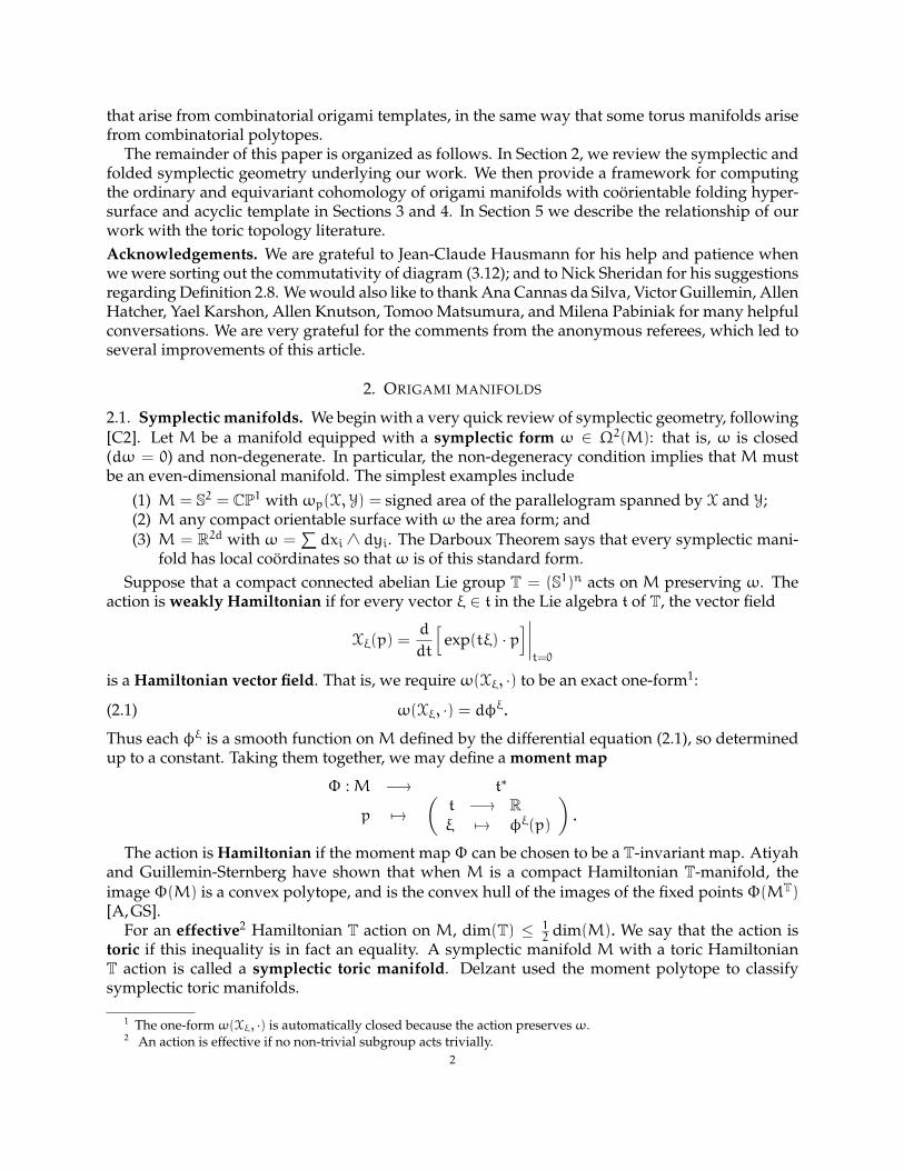
The definition of a Hamiltonian action only depends on ω being closed. Thus, in the foldedframework, we may define moment maps and toric actions exactly as in Section 2.1. For example,the action T2 S4 ⊂ C2 ⊕ R given by rotation on the C2 coordinates is Hamiltonian with momentmap

Φ(z1, z1, t) =(|z1|

2, |z2|2).

The image of this map is shown in Figure 2.3 below.An oriented origami manifold M with fold Z may be unfolded into a symplectic manifold as

follows. Consider the closures of the connected components of M \ Z, a manifold with boundarywhich consists of two copies of Z. We collapse the fibers of the null fibration by identifying theboundary points that are in the same fiber of the null fibration of each individual copy of Z. Theresult,M0 := (M\Z)∪B1∪B2, is a (disconnected) smooth manifold that can be naturally endowedwith a symplectic form which onM0 \(B1∪B2) coincides with the origami form onM\Z. Becausethis can be achieved using symplectic cutting techniques, the resulting manifold M0 is called the

3

FIGURE 2.3. The moment map image for the T2 action on S4. The image consistsof two overlapping copies of a triangle, which we have slightly unfolded. The redhypotenuse is the image of the equator S3. Every other point in the image has twoconnected components mapping to it, one from the northern hemisphere and theother from the southern.

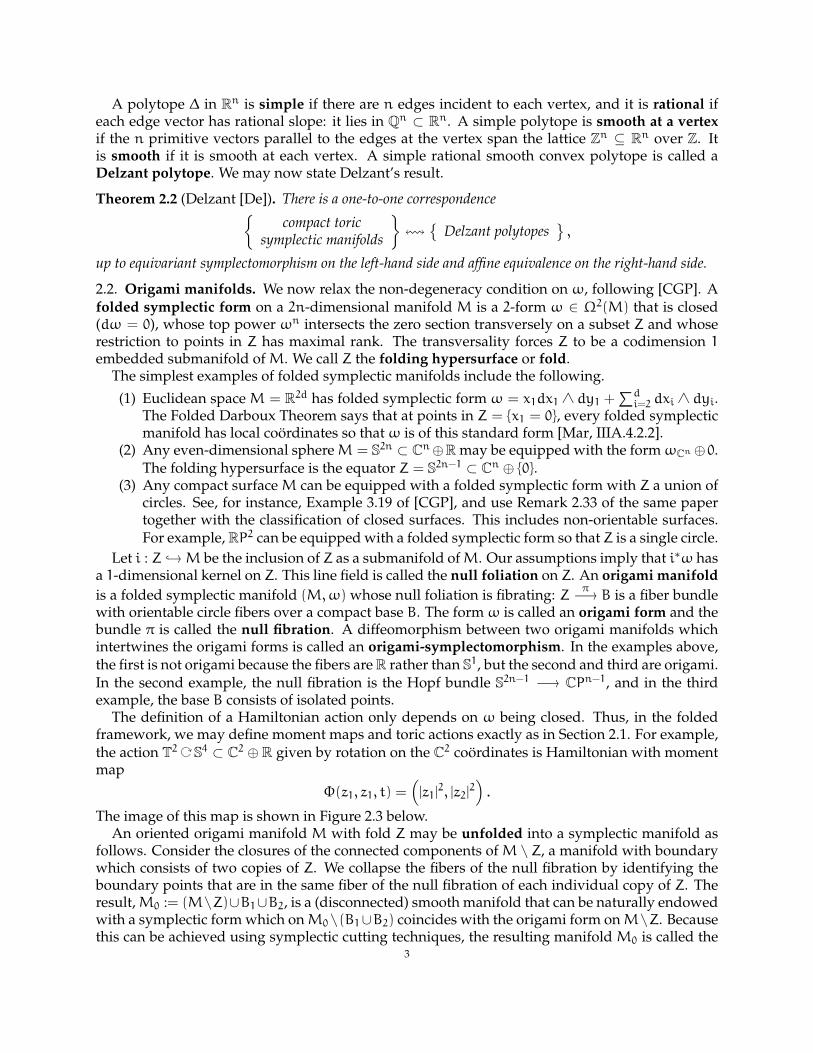
symplectic cut space (and its connected components the symplectic cut pieces), and the processis also called cutting. An example of cutting a 2-torus is shown in Figure 2.4. The symplecticcut space of a nonorientable origami manifold is the Z2-quotient of the symplectic cut space of itsorientable double cover.

FIGURE 2.4. The torus, with fold Z = S1 ∪ S1 in purple; the middle step beforecollapsing, the two copies of Z are in blue and purple; and the final cut spaceM0 =S2 ∪ S2 with B1 in red and B2 in blue.

In the example shown in Figure 2.3, unfolding the origami S4 yields CP2tCP2. This is suggestedby the image of the moment map: the moment image of each toric CP2 (regardless of orientation)is a triangle. The cut space M0 of an oriented origami manifold (M,ω) inherits a natural orienta-tion. It is the orientation on M0 induced from the orientation on M that matches the symplecticorientation on the symplectic cut pieces corresponding to the subset ofM\Zwhereωn > 0 and theopposite orientation on those pieces where ωn < 0. In this way, we can associate a + or − sign toeach of the symplectic cut pieces of an orientend origami manifold, as well as to the correspondingconnected components ofM \ Z.

Remark 2.5. In this paper we restrict to origami manifolds whose fold is coorientable: that is,the fold has an orientable neighborhood. Note that this not imply that the manifold is orientable.Indeed, for an orientableM, the condition thatωn intersects the zero section transversally impliesthat the connected components of M \ Z which are adjacent in M have opposite signs. Since M isconnected, picking a sign for one connected component ofM\Z determines the signs for all othercomponents. As a consequence, an origami manifoldMwith coorientable fold is orientable if andonly if it is possible to make such a global choice of signs for the connected components ofM \ Z.The moment image of a non-orientable origami manifold that nevertheless has coorientable foldis given in Figure 3.1.

Proposition 2.6 ([CGP, Props. 2.5 & 2.7]). Let M be a (possibly disconnected) symplectic manifold witha codimension two symplectic submanifold B and a symplectic involution γ of a tubular neighborhood U of

4

B which preserves B3. Then there is an origami manifold M such that M is the symplectic cut space of M.Moreover, this manifold is unique up to origami-symplectomorphism.

This newly-created fold Z ⊂ M involves the radial projectivized normal bundle of B ⊂ M, sowe call the origami manifold M the radial blow-up of M through (γ, B). The cutting operationand the radial blow-up operation are in the following sense inverse to each other.

Proposition 2.7 ([CGP, Prop. 2.37]). Let M be an origami manifold with cut space M0. The radialblow-up M0 is origami-symplectomorphic toM.

There exist Hamiltonian versions of these two operations which may be used to see that themoment map Φ for an origami manifold M coincides, on each connected component of M \ Zwith the induced moment map Φi on the corresponding symplectic cut piece Mi. As a result, themoment imageΦ(M) is the union of convex polytopes ∆i.

Furthermore, if the circle fibers of the null fibration for a connected component Z of the foldZ are orbits for a circle subgroup S1 ⊂ T, then Φ(Z) is a facet of each of the two polytopes cor-responding to neighboring components of M \ Z. Let us denote these two polytopes ∆1 and ∆2.We note that they must agree near Φ(Z): there is a neighborhood V of Φ(Z) in Rn such that∆1 ∩ V = ∆2 ∩ V. The condition that the circle fibers are orbits is automatically satisfied when theaction is toric, and in that case there is a classification theorem in terms of the moment data.

The moment data of a toric origami manifold can be encoded in the form of an origami tem-plate, originally defined in [CGP, Def. 3.12]. Definition 2.8 below is a refinement of that originaldefinition. The reasons for this refinement are explained in Remark 2.9.

Following [GGL, p. 5], a graph G consists of a nonempty set V of vertices and a set E of edgestogether with an incidence relation that associates an edge with its two end vertices, which neednot be distinct. Note that this allows for the existence of (distinguishable) multiple edges withthe same two end vertices, and of loops whose two end vertices are equal. We introduce someadditional notation: let Dn be the set of all Delzant polytopes in Rn and En the set of all subsets ofRn which are facets of elements of Dn.

Definition 2.8. An n-dimensional origami template consists of a graph G, called the templategraph, and a pair of maps ΨV : V −→ Dn and ΨE : E −→ En such that:

(1) if e is an edge of G with end vertices u and v, then ΨE(e) is a facet of each of the polytopesΨV(u) and ΨV(v), and these polytopes agree near ΨE(e); and

(2) if v is an end vertex of each of the two distinct edges e and f, then ΨE(e) ∩ ΨE(f) = ∅.

The polytopes in the image of the mapΨV are the Delzant polytopes of the symplectic cut pieces.For each edge e, the set ΨE(e) is a facet of the polytope(s) corresponding to the end vertices of e.We refer to such a set as a fold facet, as it is the image of the connected components of the foldinghypersurface4.

In the example of Figure 2.3, the template graph G has two vertices and one edge joining them.Both vertices are mapped to the same isosceles right angle triangle under ΨV , and the edge ismapped to the hypotenuse of that triangle under ΨE.

Remark 2.9. In the original definition of origami template, Definition 3.12 in [CGP], a templateconsisted of a pair (P,F). The set P was a collection of Delzant polytopes and F was a collectionof pairs or singletons of facets of polytopes in P, satisfying certain conditions. Roughly speaking,

3 In the noncoorientable case, the involution must satisfy additional conditions, see [CGP, Def. 2.23]. In thecoorientable case, we have B = B1 ∪ B2 and the involution γ maps a tubular neighborhood of B1 to one of B2 andvice versa.

4 A noncoorientable connected component of the folding hypersurface corresponds to a loop edge e.5

P is the image of ΨV and the sets in F assigned identifications of facets of polytopes in P in a waysimilar to that of the map ΨE. To understand the problem with this old definition we turn againto the example of Figure 2.3: the collection P would contain two identical triangles, and F wouldcontain one pair, consisting of the hypotenuses of each of the triangles. However, P is a set, andtherefore if it consists of two identical elements it actually consists of only one such element. Thesame issue exists with the pairs in F and in other examples, with F itself. Simply replacing theword set by the word multiset to allow for multiple instances of the same element gives rise to adifferent type of problem.

We thank an anonymous referee for bringing this problem to our attention.

With these combinatorial data in place, we may now state the classification theorem.

Theorem 2.10 ([CGP, Theorem 3.13]). There is a one-to-one correspondencecompact toric

origami manifolds

!

origami templates,

up to equivariant origami-symplectomorphism on the left-hand side, and affine equivalence of the image ofthe template in Rn on the right-hand side.

The orbit spaceM/T of a toric origami manifold is closely related to the origami template. WhenM is a toric symplectic manifold, then the orbit space may be identified with the correspondingDelzant polytope; this identification is achieved by the moment map. For a toric origami manifold,the orbit space is realized as the topological space obtained by gluing the polytopes inΨV(V) alongthe fold facets as specified by the map ΨE. More precisely, the orbit space is the quotient

(2.11) M/T =⊔v∈V

(v, ΨV(v))/

∼ ,

where we identify (u, x) ∼ (v, y) if there exists an edge e with endpoints u and v and the pointsx = y ∈ ΨE(e) ⊂ Rn. Again, this identification is achieved by the moment map. In simple low-dimensional examples, we can visualize the orbit space by superimposing the polytopes ΨV(v) inRn and indicating which of their facets to identify; see for instance Figures 2.3, 3.1, 3.15 and 4.11.We will see in Section 5 that there is a deformation retraction from orbit spaceM/T to the templategraph.

There is a natural description of the faces ofM/T. The facets of a polytope are well-understood.The set of facets ofM/T is ⊔

v∈VF facet of ΨV (v)F not a fold facet

(v, F)/

∼ ,

where the equivalence relation is induced by the one in (2.11). The faces of M/T are non-emptyintersections of facets in M/T, together with M/T itself. This notion of face of the orbit spaceagrees with Masuda and Panov’s definition mentioned in Section 5.

3. COHOMOLOGY CONCENTRATED IN EVEN DEGREES

We say that the origami template is acyclic if the template graph is acyclic, and therefore a tree.In this case, the leaves of the origami template are the polytopes which are images under ΨV ofthe leaves of the template graph.

In light of Remark 2.5, a toric origami manifold with coorientable folding hypersurface is ori-entable exactly when the template graph has no odd cycles. In particular, if M has an acyclicorigami template, then M is automatically orientable. Two non-acyclic origami templates are

6

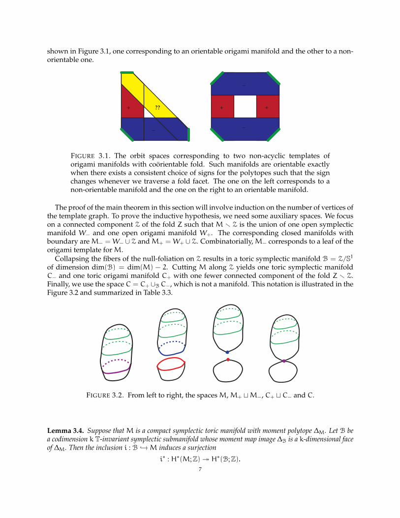
shown in Figure 3.1, one corresponding to an orientable origami manifold and the other to a non-orientable one.

+ ?? + +

–

––

FIGURE 3.1. The orbit spaces corresponding to two non-acyclic templates oforigami manifolds with coorientable fold. Such manifolds are orientable exactlywhen there exists a consistent choice of signs for the polytopes such that the signchanges whenever we traverse a fold facet. The one on the left corresponds to anon-orientable manifold and the one on the right to an orientable manifold.

The proof of the main theorem in this section will involve induction on the number of vertices ofthe template graph. To prove the inductive hypothesis, we need some auxiliary spaces. We focuson a connected component Z of the fold Z such that M r Z is the union of one open symplecticmanifold W− and one open origami manifold W+. The corresponding closed manifolds withboundary areM− =W− ∪ Z andM+ =W+ ∪ Z. Combinatorially,M− corresponds to a leaf of theorigami template forM.

Collapsing the fibers of the null-foliation on Z results in a toric symplectic manifold B = Z/S1of dimension dim(B) = dim(M) − 2. Cutting M along Z yields one toric symplectic manifoldC− and one toric origami manifold C+ with one fewer connected component of the fold Z r Z.Finally, we use the space C = C+∪BC−, which is not a manifold. This notation is illustrated in theFigure 3.2 and summarized in Table 3.3.

FIGURE 3.2. From left to right, the spacesM,M+ tM−, C+ t C− and C.

Lemma 3.4. Suppose that M is a compact symplectic toric manifold with moment polytope ∆M. Let B bea codimension k T-invariant symplectic submanifold whose moment map image ∆B is a k-dimensional faceof ∆M. Then the inclusion i : B →M induces a surjection

i∗ : H∗(M;Z) H∗(B;Z).7

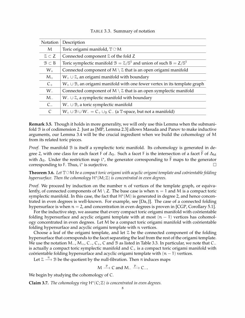
TABLE 3.3. Summary of notation

Notation Description

M Toric origami manifold, T MZ ⊂ Z Connected component Z of the fold Z

B ⊂ B Toric symplectic manifold B = Z/S1 and union of such B = Z/S1

W+ Connected component ofM \ Z that is an open origami manifold

M+ W+ ∪ Z, an origami manifold with boundary

C+ W+ ∪B, an origami manifold with one fewer vertex in its template graph

W− Connected component ofM \ Z that is an open symplectic manifold

M− W− ∪ Z, a symplectic manifold with boundary

C− W− ∪B, a toric symplectic manifold

C W+ ∪B ∪W− = C+ ∪B C− (a T-space, but not a manifold)

Remark 3.5. Though it holds in more generality, we will only use this Lemma when the submani-fold B is of codimension 2. Just as [MP, Lemma 2.3] allows Masuda and Panov to make inductivearguments, our Lemma 3.4 will be the crucial ingredient when we build the cohomology of Mfrom its related toric pieces.

Proof. The manifold B is itself a symplectic toric manifold. Its cohomology is generated in de-gree 2, with one class for each facet F of ∆B. Such a facet F is the intersection of a facet F of ∆Mwith ∆B. Under the restriction map i∗, the generator corresponding to F maps to the generatorcorresponding to F. Thus, i∗ is surjective.

Theorem 3.6. Let T M be a compact toric origami with acyclic origami template and coorientable foldinghypersurface. Then the cohomology H∗(M;Z) is concentrated in even degrees.

Proof. We proceed by induction on the number n of vertices of the template graph, or equiva-lently, of connected components of M \ Z. The base case is when n = 1 and M is a compact toricsymplectic manifold. In this case, the fact that H∗(M) is generated in degree 2, and hence concen-trated in even degrees is well-known. For example, see [Da, J]. The case of a connected foldinghypersurface is when n = 2, and concentration in even degrees is proven in [CGP, Corollary 5.1].

For the inductive step, we assume that every compact toric origami manifold with coorientablefolding hypersurface and acyclic origami template with at most (n − 1) vertices has cohomol-ogy concentrated in even degrees. Let M be a compact toric origami manifold with coorientablefolding hypersurface and acyclic origami template with n vertices.

Choose a leaf of the origami template, and let Z be the connected component of the foldinghypersurface that corresponds to the facet separating the leaf from the rest of the origami template.We use the notationM−,M+, C−, C+, C and B as listed in Table 3.3. In particular, we note that C−

is actually a compact toric symplectic manifold and C+ is a compact toric origami manifold withcoorientable folding hypersurface and acyclic origami template with (n− 1) vertices.

Let Z π−→ B be the quotient by the null-fibration. Then π induces maps

Mp−→ C andM−

p−−→ C−.

We begin by studying the cohomology of C.

Claim 3.7. The cohomology ring H∗(C;Z) is concentrated in even degrees.8

Proof of Claim 3.7. We may choose T-invariant collar neighborhoods of C− and C+ in C that de-formation retract to C− and C+ respectively. This is analogous to choosing a collar neighborhoodof Z inM, as described in the remarks just before Proposition 2.6 above.

The intersection of these neighborhoods is a collar neighborhood of B and deformation re-tracts onto B. The Mayer-Vietoris sequence for these collar neighborhoods induces a long exactsequence, in cohomology with integer coefficients

· · · // H∗(C) // H∗(C+)⊕H∗(C−) // H∗(B) // · · · .(3.8)

As C− is a compact toric symplectic manifold, Lemma 3.4 implies that H∗(C−) → H∗(B) is a sur-jection. Thus the long exact (3.8) splits into short exact sequences (again with integer coefficients)

0 // H∗(C) // H∗(C+)⊕H∗(C−) // H∗(B) // 0 .(3.9)

Note that the cohomology of C− and B is concentrated in even degrees because C− and B

are compact toric symplectic manifolds. By the induction hypothesis, the cohomology of C+ isconcentrated in even degrees. We conclude from (3.9) in odd degrees that H∗(C;Z) must be zeroin odd degrees. 4

We now look at the relationship between the cohomology of C− and that ofM−.

Claim 3.10. The quotient map p− :M− −→ C− induces a surjection in cohomology

p∗− : H∗(C−;Z) H∗(M−;Z).

In particular, H∗(C−;Z) is concentrated in even degrees, and so H∗(M−;Z) is as well.

Proof of Claim 3.10. This is an argument based on [HK, Proof of Proposition 1.3], with correc-tions following [Hau] and adjustments for integer coefficients. Consider long exact sequence inhomology with integer coefficients of the pair (C−,B)

· · · // H∗(B)i∗ // H∗(C−)

j∗// H∗(C−,B) // · · · ,(3.11)

where i : B → C− is inclusion and j : (C−, ∅) −→ (C−,B) is inclusion of the pair. We mayapply Poincare duality to Lemma 3.4 to establish that i∗ is an injection in homology with integercoefficients. Thus the long exact sequence (3.11) splits into short exact sequences. We then have acommutative diagram, with integer coefficients,

H∗−2(B)

∼= ¬

i! // H∗(C−)

∼= ­

p∗−// H∗(M−)

∼= ®

Hd−∗(M−,Z)

∼= ¯

0 // Hd−∗(B)i∗ // Hd−∗(C−)

j∗// Hd−∗(C−,B) // 0.

(3.12)

In this diagram, the manifold C− has dimension d, and B has dimension d − 2. The maps ¬ and­ are Poincare duality for the manifolds B and C− respectively, and ® is Poincare duality for themanifold M− with boundary Z. Finally, the map ¯ is (p−)∗ and is an isomorphism by excision.The left square commutes because it is the definition of the push-forward map i!.

We now check that the right square commutes. We use the fact that the Poincare duality isomor-phism is the cap product with the fundamental class. So we need to show that for any a ∈ H∗(C−),

(p−)∗(p∗−(a) _ [M−]

)= j∗

(a_ [C−]

).

9

But now, using the properties of the cap product as developed in [Hat, §3.3], we have

(p−)∗(p∗−(a) _ [M−]

)= a_ (p−)∗

([M−]

)by naturality of the cap product

= a_ j∗([C−]

)because (p−)∗

([M−]

)= j∗

([C−]

)= j∗

(a_ [C−]

)by relative naturality of the cap product, and j∗(a) = a.

Thus, the diagram commutes and we may now conclude that p∗− is a surjection. 4

Finally, we turn to the relationship between the cohomology of C and that ofM.

Claim 3.13. The quotient map p :M −→ C induces a surjection in cohomology

p∗ : H∗(C;Z) H∗(M;Z).Proof of Claim 3.13. We have long exact sequences in cohomology with integer coefficients forthe pairs (M,M−) and (C,C−) that fit into a commutative diagram

· · · // H∗(C,C−)

∼= ¬

// H∗(C)

­p∗

// H∗(C−)

®p∗−

// H∗+1(C,C−)

∼= ¯

// · · ·

· · · // H∗(M,M−) // H∗(M) // H∗(M−) // H∗+1(M,M−) // · · · .

Note that the maps ¬ and ¯ are isomorphisms by excision, and the map ® is onto by Claim 3.10.The Four Lemma (the “onto” half of the Five Lemma) states that if ¬ and ® are onto and ¯ isone-to-one, then ­ must be onto. We have this for each degree, completing the proof. 4

Claim 3.7 guarantees that the cohomology of C is concentrated in even degrees. Claim 3.13 tells

us that H∗(C;Z) p∗−→ H∗(M;Z) is surjective, and so H∗(M;Z) is necessarily concentrated in evendegrees.

Next we see how the conclusion of Theorem 3.6 can fail in the non-acyclic case.

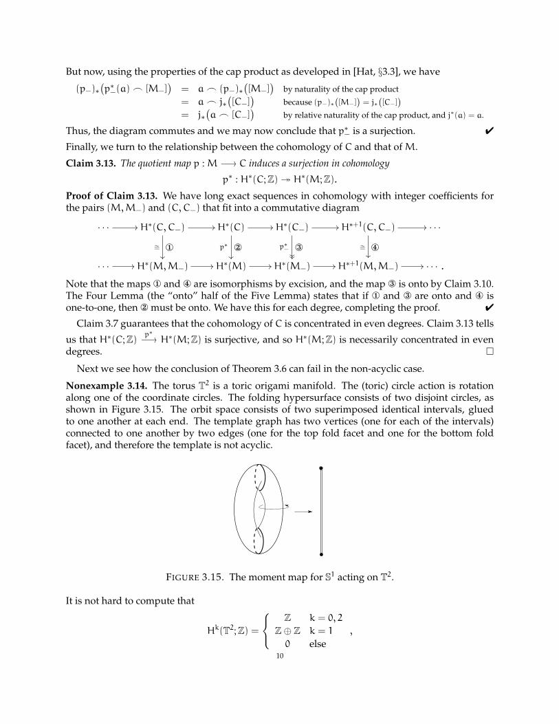
Nonexample 3.14. The torus T2 is a toric origami manifold. The (toric) circle action is rotationalong one of the coordinate circles. The folding hypersurface consists of two disjoint circles, asshown in Figure 3.15. The orbit space consists of two superimposed identical intervals, gluedto one another at each end. The template graph has two vertices (one for each of the intervals)connected to one another by two edges (one for the top fold facet and one for the bottom foldfacet), and therefore the template is not acyclic.

FIGURE 3.15. The moment map for S1 acting on T2.

It is not hard to compute that

Hk(T2;Z) =

Z k = 0, 2

Z⊕ Z k = 1

0 else,

10

and so the conclusion of Theorem 3.6 fails.

4. EQUIVARIANT COHOMOLOGY

Equivariant cohomology is a generalized cohomology theory in the equivariant category. Weuse the Borel model to compute equivariant cohomology. For the torus T, we let ET be a con-tractible space on which T acts freely. Explicitly, for a circle, we may choose ES1 to be the unitsphere S∞ in a Banach space. This is well-known to be contractible. Since T = S1 × · · · × S1 is aproduct, we may let ET be a product of infinite-dimensional spheres.

For any T-space X, the diagonal action of T on X× ET is free, and

XT = (X× ET)/Tis the Borel mixing space or homotopy quotient of X. We define the (Borel) equivariant cohomol-ogy ring to be

H∗T(X;R) := H∗(XT;R),

where H∗(−;R) denotes singular cohomology with coefficients in the commutative ring R. Thus,when X is a free T-space, we may identify

H∗T(X;R)∼= H∗(X/T;R).

At the other extreme, if T acts trivially on X, then

H∗T(X;R)∼= H∗(X× BT;R),

where BT = ET/T is the classifying space of T. Note that the cohomology of the classifying space,H∗(BT;R) ∼= H∗T(pt;R), is the equivariant cohomology ring of a point.

For any T-space X, we have the fibration

(4.1) X → XT −→ BT.The projection XT −→ BT induces the map H∗T(pt;R) −→ H∗T(X;R), which turns H∗T(X;R) into anH∗T(pt;R)-module. Natural maps in equivariant cohomology preserve this module structure.

A common tool in the computation of equivariant cohomology is the Serre spectral sequenceapplied to the fibration (4.1). This has E2-page

Ep,q2 = Hp(BT;Hq(X;R)).

This spectral sequence converges to H∗T(X;R). When X has cohomology concentrated in even de-grees, then this spectral sequence is 0 in every other row and column, and automatically collapses.In particular, the equivariant cohomology is also concentrated in even degrees.

Goresky, Kottwitz and MacPherson call a T-space X equivariantly formal if the Serre spectralsequence collapses at the E2-page [GKM]. This spectral sequence does collapse for a compact toricorigami manifold with acyclic origami template and coorientable folding hypersurface, becausethe cohomology is concentrated in even degrees (Theorem 3.6). Historically, the term “formal” hasbeen used in rational homotopy theory, and so equivariantly formal has multiple interpretations.Scull describes the relationships between these interpretations [S]. To avoid further confusion, wewill not use this term in the remainder of this paper.

Suppose that a torus T acts on a compact manifold M. Then the inclusion of the fixed pointsI :MT −→M induces a map in equivariant cohomology,

(4.2) I∗ : H∗T(M;R) −→ H∗T(MT;R).

A classical result of Borel establishes that the kernel and cokernel of I∗ are torsion submodules[Bo]. Our first step is to prove that in our set-up, I∗ is injective. We can deduce this in a variety ofways. We supply a constructive proof here that we hope adds geometric intuition in the origamisetting.

11

Theorem 4.3. Let T M be a compact toric origami with acyclic origami template and coorientable foldinghypersurface. Then the inclusion I :MT →M induces an injection in equivariant cohomology

I∗ : H∗T(M;Z) −→ H∗T(MT;Z).

Proof. We proceed by induction on the number of vertices in the template graph.

Base Case: Suppose the template graph has a single vertex. ThenM is a toric symplectic manifold.In particular, M is Kahler and has isolated fixed points. Frankel showed that H∗(M;Z) is torsionfree in this situation [Fr, Corollary 2]. The Serre spectral sequence then has no torsion at the E2page, where it collapses, so we may conclude that H∗T(M;Z) is torsion free. As the fixed points areisolated, H∗T(M

T;Z) is also torsion free, and so Borel’s classical result now implies injectivity.

Inductive Step: We now assume that the statement holds for any acyclic toric origami manifoldwith coorientable fold with at most (n− 1) vertices in its template graph.

As in the previous section, we choose a leaf of the origami template, and let Z be the connectedcomponent of the folding hypersurface that corresponds to the facet separating the leaf from therest of the origami template. We continue to use the auxiliary spacesM−,M+, C−, C+, C and B aslisted in Table 3.3.

Claim 4.4. The inclusion CT −→ C induces an injection

H∗T(C;Z) −→ H∗T(CT;Z).

Proof of Claim 4.4. We note that C− is a toric symplectic manifold, and C+ is a toric origamimanifold with fewer vertices in its template graph. Thus, in equivariant cohomology with integercoefficients,

H∗T(C−)I∗−−→ H∗T(C

T−) and H∗T(C+)

I∗+−→ H∗T(CT+)

are both injective.We now consider the equivariant Mayer-Vietoris long exact sequence for T-invariant neigh-

borhoods of C = C+ ∪ C−. The spaces C, C+, C− and B each have ordinary cohomology onlyin even degrees, and hence equivariant cohomology only in even degrees. Thus, the equivariantMayer-Vietoris long exact sequence splits into short exact sequences. We then have a commutativediagram, with integer coefficients,

0 // H∗T(C)­//

¬

H∗T(C+)⊕H∗T(C−) //

®

H∗T(B) //

0

0 // H∗T(CT) //

¯// H∗T(C

T+)⊕H∗T(CT

−) // H∗T(BT) // 0

.

The map ­ is injective because the top row is short exact. The map ® is I∗− ⊕ I∗+, and is thusinjective. Therefore, ® ­ is injective. But ® ­ = ¯ ¬. Hence, ¬ must be injective. 4

Claim 4.5. In even degrees, the map

H2∗T (C,C−) −→ H2∗T (CT, CT−)

is injective.

Proof of Claim 4.5. The pair (C,C−) is T-invariant, so we consider the long exact sequence ofthe pair in equivariant cohomology. By Claim 3.7, the cohomology of C is concentrated in evendegrees. The space C− is a toric symplectic manifold, so its cohomology is also concentrated in

12

even degrees. Thus the long exact sequence splits into a 4-term short exact sequence. This inducesa commutative diagram

0 // H2∗T (C,C−)­

//

¬

H2∗T (C) //

®

H2∗T (C−) //

H2∗+1T (C,C−) //

0

0 // H2∗T (CT, CT−)

¯// H2∗T (CT) // H2∗T (CT

−) // H2∗+1T (CT, CT−) // 0

.

The map ­ is injective because the top row is exact. The map ® is injective by Claim 4.4. Therefore,® ­ is injective. But ® ­ = ¯ ¬. Hence, ¬ must be injective. 4

Claim 4.6. The inclusionMT− →M− induces an injection H∗T(M−) → H∗T(M

T−).

Proof of Claim 4.6. Recall that C− is a toric symplectic manifold. Let f : C− −→ R be the compo-nent of its moment map that attains its maximum value on B. Let f(B) = b ∈ R. Let g :M− −→ Rbe the composition M−

p−−→ C−f−→ R. Choose ε > 0 such that there is no critical value in be-

tween b− ε and b, and so that g−1((b− ε, b]) is contained in the intersection of M− with a Moserneighborhood of Z inM.

The fact that f is a Morse-Bott function on C− with no critical values between b − ε and bguarantees that f−1((−∞, b)) and f−1((−∞, b− ε

2 ]) are homotopy equivalent. In addition, the factthat g−1((b − ε, b]) is contained in the intersection of M− with a Moser neighborhood of Z in Mguarantees that f−1((−∞, b− ε

2 ]) is homotopy equivalent toM−.We now appeal to a standard argument from equivariant symplectic geometry to conclude that

MT− = f−1

((−∞, b− ε

2

])T→ f−1

((−∞, b− ε

2

])'M−

induces an injection in equivariant cohomology. This is an inductive argument on the critical setof f, and can be copied verbatim from the proof of [TW, Theorem 2]. 4

We now consider the long exact sequence in equivariant cohomology for the pair (M,M−). Wehave shown that M− and M have cohomology and thus equivariant cohomology concentrated ineven degrees. Thus the long exact sequence splits into a 4-term short exact sequence. This inducesa commutative diagram

0 //

¬

H2∗T (M,M−)

­

// H2∗T (M)

®

// H2∗T (M−)

¯

// H2∗+1T (M,M−) //

0

0 // H2∗T (MT,MT−) // H2∗T (MT) // H2∗T (MT

−) // H2∗+1T (M,M−) // 0

.

We want to show that ® is injective. The Four Lemma (the “injectivity” half of the Five Lemma)states that if ­ and ¯ are injective and ¬ is surjective, then ® must be injective.

We first note that H∗T(M,M−) ∼= H∗T(C,C−), and H∗T(MT,MT

−) = H∗T(CT, CT

−). Thus, the map­ is injective (in even degrees) by Claim 4.5. The map ¯ is injective by Claim 4.6. The map ¬ isobviously surjective. Thus, by the Four Lemma, the map ® must be injective, as desired.

Remark 4.7. We may also derive Theorem 4.3 from work of Franz and Puppe [FP]. We describethis approach, and its further applications, in the proof of Theorem 4.12 below.

We now identify the image of I∗. Goresky, Kottwitz, and MacPherson proved that the equivari-ant cohomology of certain spaces may be described combinatorially as n-tuples of polynomialswith divisibility conditions on pairs of the polynomials [GKM, Theorem 1.22]. The description

13

applies, for example, to toric varieties [Bri, §2.2], hypertoric varieties [HH, Proposition 3.2], andcoadjoint orbits [GKM, §7.8]. In this section, we prove that the description also applies to any com-pact toric origami manifold with acyclic origami template and coorientable folding hypersurface.We begin by recalling the assumptions and results from [GKM]. The two key assumptions are

(A) The fixed point setMT consists of isolated points; and(B) The one-skeletonM1 = p ∈M | dim(T · p) ≤ 1 is 2-dimensional.

The first assumption simplifies what H∗T(MT;Z) can be. When the fixed point set consists of

isolated points, this ring is a direct product of copies of

H∗T(pt;Z) ∼= Z[x1, . . . , xn],one for each fixed point. Thus, every class can be represented as a tuple of polynomials, and thering structure is the component-wise product of polynomials.

When M is a compact Hamiltonian T-space, the second assumption ensures that the one-skeleton must consist of 2-spheres intersecting one another at the isolated fixed points. Moreover,the T-action preserves M1, and the action rotates each S2 about an axis. The image of M1 underthe moment map is an immersed graph Φ(M1) = Γ called the moment graph5 whose verticescorrespond to the fixed pointsMT and whose edges correspond to the embedded S2’s. Each edgee in Γ is labeled by the weight 6 αe ∈ t∗ by which T acts on e. Indeed, the moment map sendsthe corresponding S2 to a line segment parallel to the weight αe. The embedding of the graphΓ encodes in this way the isotropy data, denoted α. In this framework, we have the followingdescription of H∗T(M;Q).

Theorem 4.8 (Goresky-Kottwitz-MacPherson [GKM]). SupposeM is a compact Hamiltonian T-spacesatisfying conditions (A) and (B) above. Then I∗ is injective

I∗ : H∗T(M;Q) → H∗T(MT;Q) ∼=

⊕p∈MT

H∗T(pt;Q),

and its image consists of

(4.9)(fp) ∈

⊕p∈MT

H∗T(pt;Q)∣∣∣ αe∣∣(fp − fq) for each edge e = (p, q) in Γ

.

We will refer to these divisibility conditions as the GKM description.

Remark 4.10. For a Hamiltonian T-space, assumption (A) guarantees that I∗ is injective in equi-variant cohomology with integer coefficients. We may strengthen assumption (B) to guaranteethat the GKM description holds over Z. A stronger set of assumptions are described in [HHH, §3];they include the existence of a cell decomposition of the manifold. In particular, for HamiltonianT-spaces with isolated points, Morse theory can be applied to a generic component of the momentmap to establish that these stronger assumptions boil down to local topological properties thatmust be checked at the fixed points. These can then be verified for symplectic toric manifolds andfor coadjoint orbits.

As we have seen, the moment map for a toric origami manifoldM does not necessarily produceMorse functions onM. We do not know if there is a cell decomposition of a toric origami manifoldthat would allow us to apply techniques from [HHH].

A key technical tool in the proof of Theorem 4.8 is the Chang-Skjelbred Lemma [CS, Lemma 2.3].Let J : MT −→ M1 denote the inclusion of the fixed points into the one-skeleton. The Chang-Skjelbred Lemma states that I∗(H∗T(M)) = J∗(H∗T(M1)). Since the one-skeleton consists of S2’s, we

5 The moment graph Γ is sometimes called the GKM graph. It is not the template graph.6 This is well-defined up to a sign, which is sufficient for our purposes.

14

must understand H∗T(S2). It is a simple calculation to check that each S2 contributes one of thedivisibility conditions in (4.9).

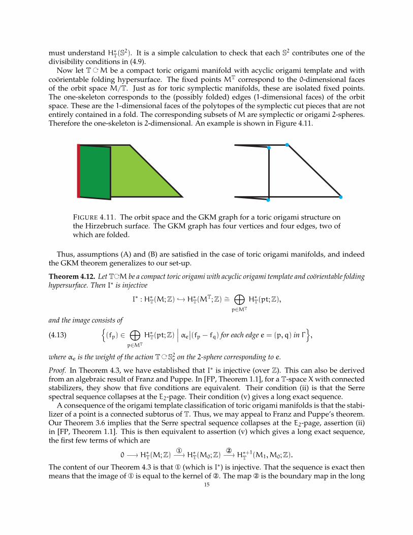
Now let T M be a compact toric origami manifold with acyclic origami template and withcoorientable folding hypersurface. The fixed points MT correspond to the 0-dimensional facesof the orbit space M/T. Just as for toric symplectic manifolds, these are isolated fixed points.The one-skeleton corresponds to the (possibly folded) edges (1-dimensional faces) of the orbitspace. These are the 1-dimensional faces of the polytopes of the symplectic cut pieces that are notentirely contained in a fold. The corresponding subsets ofM are symplectic or origami 2-spheres.Therefore the one-skeleton is 2-dimensional. An example is shown in Figure 4.11.

FIGURE 4.11. The orbit space and the GKM graph for a toric origami structure onthe Hirzebruch surface. The GKM graph has four vertices and four edges, two ofwhich are folded.

Thus, assumptions (A) and (B) are satisfied in the case of toric origami manifolds, and indeedthe GKM theorem generalizes to our set-up.

Theorem 4.12. Let T M be a compact toric origami with acyclic origami template and coorientable foldinghypersurface. Then I∗ is injective

I∗ : H∗T(M;Z) → H∗T(MT;Z) ∼=

⊕p∈MT

H∗T(pt;Z),

and the image consists of

(4.13)(fp) ∈

⊕p∈MT

H∗T(pt;Z)∣∣∣ αe∣∣(fp − fq) for each edge e = (p, q) in Γ

,

where αe is the weight of the action T S2e on the 2-sphere corresponding to e.

Proof. In Theorem 4.3, we have established that I∗ is injective (over Z). This can also be derivedfrom an algebraic result of Franz and Puppe. In [FP, Theorem 1.1], for a T-space Xwith connectedstabilizers, they show that five conditions are equivalent. Their condition (ii) is that the Serrespectral sequence collapses at the E2-page. Their condition (v) gives a long exact sequence.

A consequence of the origami template classification of toric origami manifolds is that the stabi-lizer of a point is a connected subtorus of T. Thus, we may appeal to Franz and Puppe’s theorem.Our Theorem 3.6 implies that the Serre spectral sequence collapses at the E2-page, assertion (ii)in [FP, Theorem 1.1]. This is then equivalent to assertion (v) which gives a long exact sequence,the first few terms of which are

0 −→ H∗T(M;Z) ¬−→ H∗T(M0;Z)­−→ H∗+1T (M1,M0;Z).

The content of our Theorem 4.3 is that ¬ (which is I∗) is injective. That the sequence is exact thenmeans that the image of ¬ is equal to the kernel of ­. The map ­ is the boundary map in the long

15

exact sequence of the pair (M1,M0). Thus we have

· · · −→ H∗T(M∗1 ;Z)

®−→ H∗T(M0;Z)­−→ H∗+1T (M1,M0;Z) −→ · · · .

The kernel of ­ is then equal to the image of ®, which is the image of the equivariant cohomologyof the one-skeleton inH∗T(M0;Z). The fact that the one-skeleton consists of symplectic and origami2-spheres means that each S2 contributes one of the divisibility conditions in (4.13).

In Section 3, we proved that H∗(M;Z) is concentrated in even degrees. We do not have a Morsefunction on M that would allow us to compute the ranks of these cohomology groups. Withour explicit description of H∗T(M;Z), it is possible in examples to determine the ranks and ringstructure of H∗(M;Z). This is a consequence of the collapse of the Serre spectral sequence, whichimplies that

H∗(M;Z) ∼= H∗T(M;Z)⊗H∗T(pt;Z) Z.

Example 4.14. The 2n-sphere S2n may be endowed with toric origami structure whose templategraph has two vertices and a single edge between them. Each of the two vertices maps to a then-simplex in Rn with an orthogonal corner at the origin; that is, a simplex with vertices the originand the standard basis vectors ei = (0, . . . , 1, . . . , 0) with a single 1 in the ith coordinate and 0selsewhere. The edge maps to the fold facet by which these two polytopes are glued together:the (n − 1)-simplex with vertices the ei, opposite the origin. The orbit space for S4 is shown inFigure 2.3.

Thus the toric action has 2 fixed points, which we denote N and S (for the north and southpoles). There are n edges in the GKM graph, each joining Φ(N) and Φ(S). We can identifyH∗T(pt;Z) = Z[x1, . . . , xn]. From the representation of the orbit space in Rn we can see that theT-action on the sphere mapping to the ith coordinate line in Rn has weight xi. Theorem 4.12 statesthat

I∗(H∗T(S2n;Z)) =(fN, fS) ∈ Z[x1, . . . , xn]⊕ Z[x1, . . . , xn]

∣∣∣ xi∣∣(fN − fS) for i = 1, . . . , n.

From this, we can find a module basis (for H∗T(S2n;Z) as an H∗T(pt;Z)-module) with two elements

I∗(1) = (1, 1) and I∗(π) = (x1 · · · xn, 0),

where 1 ∈ H0T(S2n;Z) and π ∈ H2nT (S2n;Z).

Nonexample 4.15. We revisit Nonexample 3.14, of a toric circle action on a torus. The circle actionis free, and so has no fixed points. Nevertheless, we may compute

HkS1(T2;Z) = Hk(T2/S1;Z) = Hk(S1) =

Z k = 0, 1

0 else.

In particular, the conclusion of Theorem 4.3 cannot hold.

5. TORIC ORIGAMI MANIFOLDS ARE LOCALLY STANDARD

Toric topology is the study of topological analogues of toric symplectic manifolds and toricvarieties. The symplectic or algebraic structure is dropped, and the focus is the existence of aneffective smooth action of a torus half the dimension of the manifold. Examples of such topologicalanalogues, from most restrictive to most general, are toric manifolds [DJ] (referred to by someauthors as quasitoric manifolds), topological toric manifolds [IFM] and torus manifolds [Mas].

We now show that acyclic toric origami manifolds fit into the framework of torus manifolds,and that Theorem 3.6 also follows from the work of Masuda and Panov on the cohomology oftorus manifolds [MP]. Their theory is more general and their proofs algebraic.

16

A torus manifold is a 2n-dimensional closed connected orientable smooth manifoldMwith aneffective smooth action of an n-dimensional torus Tn with non-empty fixed set. A torus manifoldM is said to be locally standard if every point in M has an invariant neighbourhood U weaklyequivariantly diffeomorphic to an open subsetW ⊂ Cn invariant under the standard Tn-action onCn. The adverb ‘weakly’ means that there is an automorphism ρ : T −→ T and a diffeomorphismf : U −→W such that

f(ty) = ρ(t)f(y)

for all t ∈ T, y ∈ U.Compact symplectic toric manifolds are locally standard [De, Proof of Lemme 2.4]. Next we will

prove that toric origami manifolds with coorientable folding hypersurface are also locally stan-dard. Toric origami manifolds with non-coorientable components of the fold are not locally stan-dard. Indeed, an invariant neighborhood of a point on a non-coorientable component of the foldis a bundle of Mobius bands over the corresponding connected component of B [CGP, Rmk. 2.26],which is not equivariantly diffeomorphic to an invariant open subset of Tn Cn.

Lemma 5.1. Suppose that (M,Z,ω,Φ,T) is a toric origami manifold with coorientable folding hypersur-face. ThenM is locally standard.

Proof. The argument used in [De, Proof of Lemme 2.4] to prove that compact symplectic toricmanifolds are locally standard does not use compacteness of the manifold, and therefore appliesdirectly to the manifoldM \ Z.

Next, we check the ‘locally standard’ condition on a point p ∈ Z on the fold. We use a Mosermodel, as defined in [CGP, Def. 2.12], for a neighborhood of p. As remarked in [CGP], such Mosermodels exist for orientable origami manifolds. What is necessary for the local existence of theMoser model near a single component of the fold is simply the coorientability of that piece of thefold. Thus, we may assume that p ∈ Z has a neighborhood with a Moser model.

Let Zp denote the connected component of Z containing p. The local Moser model is an equi-variant diffeomorphism

ϕ : Zp × (−ε, ε) −→ U,

where ε > 0 and U is a tubular neighborhood of Zp, such that ϕ(x, 0) = x for all x ∈ Zp. Thesymplectic form can be written in these coordinates, but we do not need that here.

We now consider the null-fibration S1 → Zpπ−→ Bp. This is a principal S1-bundle, and the

base space is a compact symplectic toric manifold of dimension (2n − 2). Let b = π(p). Compacttoric symplectic manifolds are locally standard. Choose a neighborhood V of b ∈ Bp that is weaklyequivariantly diffeomorphic to an open subsetW ⊂ Cn−1 that is invariant with respect to the stan-dard Tn−1-action on Cn−1. By possibly passing to a smaller neighborhood of b, we may assumethat the bundle over V is trivial, V × S1 π−→ V . Thus, we have an equivariant neighborhood

V × S1 × (−ε, ε)

of p ∈ Zp. Under this identification, the action of Tn splits into the Tn−1 action on V , and S1 actingon itself by multiplication on the S1. We may embed S1 × (−ε, ε) as an open annulus A ⊂ C byequivariant diffeomorphism. Therefore V × S1 × (−ε, ε) is weakly equivariantly diffeomorphic toan open subsetW×A ⊂ Cn−1×C that is invariant with respect to the coordinate Tn-action on thevector space Cn. 7

7 An alternative proof for this Lemma was pointed out to us by one of the referees: it uses the fact that any subman-ifold of M consisting of points with the same isotropy subgroup is tranverse to the folding hypersurface Z. This factrelies strongly on the coorientability hypothesis.

17

A key player in Masuda and Panov’s work on torus manifolds is the orbit space Q = M/T,which in the origami framework is closely related to the origami template, as explained at theend of Section 2. Masuda and Panov define the faces of the orbit space using their notion ofcharacteristic submanifold. The orbit space is then called face-acyclic if every face F (including Qitself) is acyclic: that is, it has H∗(F) = 0.

Note that the orbit space M/T deformation retracts onto the template graph: each polytopeΨV(v) deformation retracts onto a point in its center and rays from that point to each of the foldfacets of that polytope. This can be done so that when two polytopes are glued along a fold facet,the rays from the center points of the two polytopes join at the fold facet: the two rays now forma line between the center points of the two polytopes. Viewing the center points of the polytopesas vertices of a graph and the lines joining them as edges, we recover the template graph. Anexample is provided in Figure 5.2.

+ ?? + +

–

––

+ ?? + +

–

––

+ ?? + +

–

––

FIGURE 5.2. Each polytope deformation retracts onto a central point and rays to-wards the fold facets. The orbit space M/T deformation retracts onto the templategraph.

Theorem 5.3. Suppose that (M,Z,ω,Φ,T) is a toric origami manifold such that each connected compo-nent of the folding hypersurface is coorientable. ThenM/T is face-acyclic if and only if the origami templateis acyclic.

Proof. The orbit space M/T deformation retracts onto the template graph, and any face F of M/Tdeformation retracts onto a subgraph: the vertices of this subgraph correpond to the polytopesΨV(v) which have non-empty intersection with F, its edges are the fold facets ΨE(e) which havenon-empty intersection with F.

Being homotopy equivalent to a (sub)graph, a face of M/T will be acyclic if and only if that(sub)graph has no cycles, and therefore M/T is face-acyclic exactly when the template graph hasno cycles.

We now can derive our Theorem 3.6 from Masuda and Panov’s work: they prove that face-acyclic locally standard torus manifolds have no odd-degree cohomology [MP, Theorem 9.3].While our proofs have very different flavors, it is interesting to note that a crucial ingredient intheir proof is their [MP, Lemma 2.3], which is closely related to our Lemma 3.4, as described inRemark 3.5.

REFERENCES

[A] M. Atiyah, “Convexity and commuting Hamiltonians.” Bull. London Math. Soc. 14 (1982): 1–15.[Bo] A. Borel, Seminar on transformation groups. With contributions by G. Bredon, E. E. Floyd, D. Montgomery, R.

Palais. Annals of Mathematics Studies, No. 46 Princeton University Press, Princeton, NJ, 1960.[Bri] M. Brion, “Piecewise polynomial functions, convex polytopes and enumerative geometry.” Parameter spaces

(Warsaw, 1994), 25–44, Banach Center Publ., 36, Polish Acad. Sci., Warsaw, 1996.18

[C2] A. Cannas da Silva, Lectures on Symplectic Geometry, Lecture Notes in Mathematics 1764, corrected 2nd printing,Springer, 2008.

[CGP] A. Cannas da Silva, V. Guillemin, A.R. Pires, “Symplectic origami.” IMRN 2011 (2011) no. 18: 4252–4293.[CS] T. Chang, T. Skjelbred, “Topological Schur lemma and related results.” Bull. Amer. Math. Soc. 79 (1973): 1036–

1038.[Da] V. Danilov, “The geometry of toric varieties.” Russian Math. Surveys 33 (1978) no. 2: 97–154.[DJ] M. Davis, T. Januskiewicz, ”Convex polytopes, Coxeter orbifolds and torus actions.” Duke Math. Journal 62

(1991) no. 2: 417-451.[De] T. Delzant, “Hamiltoniens periodiques et images convexes de l’application moment.” Bull. Soc. Math. France

116 (1988): 15–339.[Fr] T. Frankel, “Fixed points and torsion on Kahler manifolds.” Ann. of Math. (2) 70 (1959): 1–8.[FP] M. Franz and V. Puppe, “Exact cohomology sequences with integral coefficients for torus actions.” Transform.

Groups 12 (2007), no. 1: 65–76.[GKM] M. Goresky, R. Kottwitz, R. MacPherson, “Equivariant cohomology, Koszul duality, and the localization theo-

rem.” Invent. Math. 131 (1998), no. 1: 25–83.[GGL] R.L. Graham, M. Grotschel, L. Lovasz, ed. Handbook of Combinatorics, Volume 1, MIT Press, 1995.[GLS] V. Guillemin, E. Lerman, S. Sternberg, Symplectic Fibrations and Multiplicity Diagrams, Cambridge University

Press, Cambridge, 1996.[GS] V. Guillemin, S. Sternberg, “Convexity properties of the moment mapping.” Invent. Math. 67 (1982): 491–513.[HHH] M. Harada, A. Henriques, T. Holm, “Computation of generalized equivariant cohomologies of Kac-Moody

flag varieties.” Adv. Math. 197 (2005), no. 1: 198–221.[HH] M. Harada and T. Holm, “The equivariant cohomology of hypertoric varieties and their real loci.” Comm. Anal.

Geom. 13 (2005), no. 3, 527–559.[Hat] A. Hatcher, Algebraic Topology, Cambridge University Press (2002).[Hau] J.-Cl. Hausmann, personal communication.[HK] J.-Cl. Hausmann and A. Knutson, “Cohomology rings of symplectic cuts.” Differential Geom. Appl. 11 (1999),

no. 2: 197–203.[IFM] H. Ishida, Y. Fukukawa and M. Masuda, “Topological toric manifolds.” Mosc. Math. J. 13 (2013) no. 1: 57–98.[J] J. Jurkiewicz, “Chow ring of projective nonsingular torus embedding.” Colloq. Math. 43 (1980), no. 2: 261–270.[Mas] M. Masuda, “Unitary toric manifolds, multi-fans and equivariant index.” Tohoku Math. J. 51:2 (1999): 237–265.[MP] M. Masuda, T. Panov, “On the cohomology of torus manifolds.” Osaka J. Math. 43 (2006), no. 3: 711–746.[Mar] J. Martinet, “Sur les singularites des formes differentielles.” Ann. Inst. Fourier (Grenoble) 20 (1970): 95–178.[S] L. Scull, “Equivariant formality for actions of torus groups.” Canad. J. Math. 56 (2004), no. 6: 1290–1307.[TW] S. Tolman, J. Weitsman, “On the cohomology rings of Hamiltonian T -spaces.” Northern California Symplectic

Geometry Seminar, part of Amer. Math. Soc. Transl. Ser. 2, 196, Amer. Math. Soc., Providence, RI (1999): 251–258.

DEPARTMENT OF MATHEMATICS, MALOTT HALL, CORNELL UNIVERSITY, ITHACA, NEW YORK 14853-4201, USAE-mail address: tsh@math.cornell.eduURL: http://www.math.cornell.edu/˜tsh/

DEPARTMENT OF MATHEMATICS, MALOTT HALL, CORNELL UNIVERSITY, ITHACA, NEW YORK 14853-4201, USAE-mail address: apires@math.cornell.eduURL: http://www.math.cornell.edu/˜apires/

19