Embed Size (px)
Citation preview
IEEE TRANSACTIONS ON KNOWLEDGE AND DATA ENGINEERING, VOL. ?, NO. ?, ? ? 1
The Threshold Algorithm: from Middleware
Systems to the Relational Engine
Nicolas Bruno Hui(Wendy) Wang
Microsoft Research University of British Columbia
[email protected] [email protected]
DRAFT
IEEE TRANSACTIONS ON KNOWLEDGE AND DATA ENGINEERING, VOL. ?, NO. ?, ? ? 2
Abstract
The answer to a top-k query is anorderedset of tuples, where the ordering is based on how closely
each tuple matches the query. In the context of middleware systems, new algorithms to answer top-k
queries have been recently proposed. Among these, the Threshold Algorithm, orTA, is the most well
known instance due to its simplicity and memory requirements. TA is based on an early-termination
condition and can evaluate top-k queries without examining all the tuples. This top-k query model
is prevalent over middleware systems, but also over plain relational data. In this work we analyze
the challenges that must be addressed to adaptTA to a relational database system. We show that,
depending on the available indexes, many alternativeTA strategies can be used to answer a given query.
Choosing the best alternative requires a cost model that canbe seamlessly integrated with that of current
optimizers. In this work we address these challenges and conduct an extensive experimental evaluation
of the resulting techniques by characterizing which scenarios can take advantage ofTA-like algorithms
to answer top-k queries in relational database systems.
Index Terms
H.2.4 [Database Management]: Systems—Query processing; Relational databases; H.3.3 [Informa-
tion Storage and Retrieval]: Information Search and Retrieval—Retrieval models; Search process.
I. INTRODUCTION
The answer to atop-k query is anorderedset of tuples, where the ordering is based on how
closely tuples match the given query. Thus, the answer to a top-k query does not include all
tuples that “match” the query, but instead only the bestk such tuples. Consider for instance a
multimedia system with an attributeRC that contains information about the color histogram of
each picture, and another attributeRS with information about shapes. To obtain a few pictures
that feature red circles, we might ask a top-10 query with a scoring function that combines (e.g.,
using a weighted average) the redness score of each picture (provided byRC), with its “circle”
score (provided byRS). Other applications that rely on this model are information retrieval
systems [1], data broadcast scheduling [2], and restaurantselection systems [3].
One way to evaluate a top-k query is to process all candidate tuples in the database, calculate
their scores, and return thek tuples that score the highest (we called this ascan-basedapproach
since it requires to sequentially examine all tuples in the database). In some scenarios, however,
we can evaluate top-k queries more efficiently.
DRAFT
IEEE TRANSACTIONS ON KNOWLEDGE AND DATA ENGINEERING, VOL. ?, NO. ?, ? ? 3
Reference [4] introduced the Threshold Algorithm, orTA, for processing top-k queries in the
context of middleware systems. A middleware system in [4] consists ofm autonomous data
sources that provide access to attributes{c1, . . . , cm} of all objects in the system. Such sources
can be explored usingsorted access(in which attribute values are returned in descending order
for a given attribute scoring function) andrandom access(in which the value of an object’s
attribute is obtained by providing the object’s identifier). A top-k query in such scenario is given
by a monotonic functionF (e.g., min or average) that aggregates the individual attribute scores.
In a middleware system, we cannot efficiently combine the information about an object that
is scattered across data sources. Toreconstructan object from its identifier, we need to issue
several random accesses to the data sources (typically one random access per attribute), which is
expensive. For that reason, scan-based algorithms are not an efficient alternative in middleware
systems. The distinguishing characteristic ofTA is the use of an early-termination condition that
allows returning the top-k elementswithout examining the values of all tuples in the system.
At the same time,TA requires a bounded amount of memory to operate (independentof the
data size and distribution) and is straightforward to implement1. TA was shown to beinstance
optimal among all algorithms that use random and sorted access capabilities [4].
In recent years, there has been an increasing amount of research (e.g., [5], [6], [7], [8]) that
focused on answering top-k queries in the context of relational database management systems,
or RDBMS (we explain these previous efforts in the next section). These recent advances pose
the intriguing question of whetherTA, which was designed specifically for middleware systems,
is suitable for a RDBMS. On one hand, the early termination condition, memory guarantees,
and overall simplicity ofTA are very appealing. On the other hand, thereconstruction problem
of scan-based algorithms is not that severe in a RDBMS. In fact, we can centralize all the
information about an object in a table or materialized view so that each row contains all attributes
of the object being represented. Therefore, we do not need toissue expensive random access
probes to retrieve missing attribute values as it is the casein middleware systems. In this work
we critically examine whenTA-like algorithms are a good alternative in a RDBMS, and when
they fail to provide any benefit.
1Alternative algorithms, such as NRA or CA [4], require in theworst case as much memory as the data size itself, and rely
on complex bookkeeping which make implementations non-trivial.
DRAFT
IEEE TRANSACTIONS ON KNOWLEDGE AND DATA ENGINEERING, VOL. ?, NO. ?, ? ? 4
In Section II we first define the top-k query problem. We then determine, in Section III,
how the different components ofTA reconcile with algorithms and data structures present in a
RDBMS, and what are the main differences between the middleware solution and its relational
counterpart. As we will see, depending on the available indexes, many alternative TA-strategies
are possible. Not only the number of such strategies is typically very large, but the cost of each
alternative can vary drastically. (TA strategies can be either orders of magnitude more efficient or
more expensive than scan-based alternatives.) It is then crucial to develop a cost model that helps
the query optimizer decide among allTA strategies and the traditional scan-based alternative. In
the second half of Section III we develop a cost model that uses power-laws to approximate the
cost of aTA strategy in a way that it is easy to incorporate to an existingoptimizer. Finally, In
Section IV we discuss some extensions to the basic model and we report extensive experimental
results in Section V.
A. Related Work
There has been a significant amount of research on top-k queries in the recent literature. Al-
though in this work we refer to the middleware algorithm asTA [4], we note that slight variations
of TA were independently proposed in [9] and [10]. Later, references [11] and [3], among others,
extended the basic algorithms to address middleware sources that restrict their access capabilities.
Reference [12] conducted an experimental evaluation of an earlier algorithm [13] that efficiently
answers top-k queries. The authors implemented the algorithm in the Garlic middleware system
and explored its strengths and weaknesses. Later, reference [4] showed thatTA is asymptotically
more efficient than the algorithm in [13].
Reference [6] presented techniques to evaluate top-k queries through traditional SQLorder
by clauses. These techniques leverage the fact that whenk is relatively small compared to the size
of the relation, specialized sorting (or indexing) techniques that can produce the first few values
efficiently should be used. However, in order to apply these techniques for the types of scoring
functions that we consider in this work, we need to first evaluate the scoring function for each
database object. Hence, these strategies require a sequential scan of all data as a preprocessing
step.
References [7], [8] proposed a different approach to evaluate top-k selection queries in database
systems: a thin layer on top of the database system maps top-k selection queries into tight
DRAFT
IEEE TRANSACTIONS ON KNOWLEDGE AND DATA ENGINEERING, VOL. ?, NO. ?, ? ? 5
range queries that are expected to contain the top-k answers. While [7] uses multidimensional
histograms to do the mapping, reference [8] relies on samples. If some of the top-k results are
missed by the approximated range query, [7] restarts the top-k query with a larger range (or a
full sequential scan is performed). In contrast to [7], the techniques presented in this work do
not result in restarts and therefore avoid sequential scans.
Reference [5] focused on a problem closely related to ours, which is integrating top-k join
queries in relational databases. The assumption in that work is that the contribution of each table
to the overall scoring function depends on just one attribute in the table (or, at least, that we can
scan each table in descending order of the “partial score” associated with the table). Therefore,
the main problem consists of introducing non-blocking rank-aware join operators and reorder
the joins in the final execution plan to minimize the overall cost. In contrast, we focus on multi-
attribute top-k queries over a single table, and investigate how we can exploit indexes to evaluate
such queries efficiently. As a motivating example, consideran art museum that displays both
pictures and photographs. We might want to locate a room in the museum that contains both a
picture with red circles and a photograph with blue squares (let us define the combined score of
a room as the average score of its best “red-circle” picture and “blue-square” photograph). We
might then issue the following query:
SELECT TOP 1 PI.room location
FROM pictures PI, photographs PH
WHERE PI.room id = PH.room id
ORDER BY 0.5*( red circle(PI) + blue square(PH) )
The techniques in [5] would efficiently answer this query provided that there is a mechanism to
retrieve pictures in descending order of“red circle” values (similarly, photographs in descending
order of“blue square” values). As we saw in the introduction, the “redcircle” score of a picture
is not given by any of its attributes in isolation, but instead by another scoring function on
multiple attributes. Therefore, if we were to apply the techniques in [5], we would need to first
scan bothpictures andphotographs tables, then sort all the objects by their respective
partial scoring functions, store these partial scores as computed columns, and finally pipeline this
intermediate result to the rank-aware join operator of [5].Of course, scanning and sorting the
leaf nodes in the plan can easily become the bottleneck. In this paper we show how to efficiently
process such sub-queries. We believe that our work and [5] complement each other nicely: the
DRAFT
IEEE TRANSACTIONS ON KNOWLEDGE AND DATA ENGINEERING, VOL. ?, NO. ?, ? ? 6
resulting execution plans returned by our techniques can beseen as the leaf nodes in the join
plans of [5], thus extending the set of top-k queries that can be evaluated without scanning the
underlying tables.
Recently, reference [14] proposed to makeTA cost-aware by explicitly modeling the cost
of sorted accesses and allowingTA to vary the relative accessspeedto the sorted sources
accordingly. For instance, if a source suddenly becomes very slow, the algorithm in [14] would
reduce the frequency that this source is accessed, therefore increasing the efficiency of the
whole algorithm. Reference [14] has some similarities withour work, but it is still focused
on middleware scenarios and therefore does not take into account the specific characteristics
of relational database systems. First, reference [14] assumes that sorted access costs fluctuate
widely and are in general much larger than random access costs. In contrast, in a RDBMS the
cost of (random or sequential) accesses are very predictable and do not fluctuate significantly
(additionally, the cost of a random access is known to be muchhigher than that of a sequential
access in a RDBMS). Second, reference [14] adapts the algorithm on the fly, while the query
is executing. In contrast, our techniques exploit global statistics that are present in a RDBMS
to statically choose the best execution plan. Finally, in contrast with a middleware scenario, our
work recognizes that there might be different ways to accomplish a random or sorted access
depending on the set of available indexes in the RDBMS, and this choice can greatly impact
the overall efficiency of the resulting algorithm. We believe, however, that our work can benefit
from the ideas in [14]. In fact, after the best plan has been picked, we could use the techniques
in [14] to vary the relative speed at which the chosen indexesare accessed and further improve
the efficiency of the algorithm (see Section IV-B for more details).
II. PROBLEM STATEMENT
We next review theTA algorithm for middleware systems and formalize our problemin the
context of a RDBMS.
A. TA Algorithm
Consider a top-k query over attributesc1, . . . , cm and a scoring functionF (s1(c1), . . . , sm(cm)),
wheresi is the scoring function of attributeci. Suppose that sourceRi handles attributeci. Below
we summarize theTA algorithm to obtain thek objects with the best scores.
DRAFT
IEEE TRANSACTIONS ON KNOWLEDGE AND DATA ENGINEERING, VOL. ?, NO. ?, ? ? 7
1) Do sorted access in parallel to each of them sources. As an objectO is seen under sorted
access in sourceRi, do random access to the other sourcesRj and calculate the remaining
attribute scoressj of object O. Compute the overall scoreF (s1, . . . , sm) of objectO. If
this value is one of thek highest seen so far, remember objectO and its score (break ties
arbitrarily).
2) Let sLi be the score of the last object seen under sorted access for sourceRi. Define the
threshold valueT to be F (sL1 , . . . , sL
m). If the score of the current top-k object is worse
thanT , return to step 1.
3) Return the current top-k objects as the query answer.
Correctness ofTA follows from the fact that the threshold valueT represents the best possible
score that any object not yet seen can have, andTA stops when it can guarantee that no unseen
object might have a better score than the current top-k ones. The algorithm in [4] was later
extended to support scenarios in which some sources cannot provide sorted access. In such
situations, we need to replacesLi with the maximum possible score for each sourceRi that
cannot provide sorted access. The correctness and instanceoptimality of TA are preserved in
this case as well.
B. Server Side Problem Statement
In the context of a RDBMS, we focus on the following problem. Consider tableR with
attributesc1, . . . , cm (and possibly other attributes not mentioned in the query).We specify a
top-k query inSQL as follows2:
SELECT TOP(k) c1, ..., cm
FROM R
WHERE P
ORDER BY F(s1(c1), ..., sm(cm)) DESC
whereP is an filter predicate,F is a monotonic aggregate function, andsi are individual attribute
scoring functions. In current database systems, the best way to evaluate such top-k query is a
scan-based approach. Conceptually, we first obtain the bestexecution plan for the following
query:
2Queries might have additional columns in theSELECT clause that are not present in theORDER BY clause. This results in
minor variations to our techniques, but we omit such detailsfor simplicity.
DRAFT
IEEE TRANSACTIONS ON KNOWLEDGE AND DATA ENGINEERING, VOL. ?, NO. ?, ? ? 8
SELECT c1,..., cm, F(s1(c1),..., sm(cm)) as S
FROM R
WHERE P
and then we apply apartial-sort3 operator on columnS on top of this execution plan. If no
predicateP is specified, the best execution plan consists of a sequential scan over tableR, or over
the smallest-sized index that covers all columns of interest if any is available (since columns have
different widths, the smallest-sized index need not agree with the one with the fewest number of
columns). In the next section we focus on queries with no filter predicateP, and in Section IV
we explain how to lift this restriction.
Analogous to the middleware scenario, execution alternatives adapted fromTA might some-
times outperform the scan-based approach used in current database systems. We next investigate
how to adaptTA to work in a RDBMS, what are the differences and similaritieswith respect to
the middleware case, and whenTA-based strategy can be beneficial in this new scenario.
III. TA IN A RDBMS
We now explain howTA can be adapted to work in the context of a RDBMS. Indexes are the
most widely used mechanism to improve performance in a RDBMS, and our adaptation of the
TA algorithm is based on such physical structures. Specifically, we simulateeach autonomous
source in the originalTA with suitable index strategies that support the sorted and random access
interfaces.
Recall thatTA’s scoring function is a monotonic aggregate of individual attribute scoring
functions. If we do not restrict these attribute scoring functions in any way, in general we would
need to access all tuple values and sort them by each attribute scoring function before providing
the first sorted access. This preprocessing step is expensive and defeats the purpose ofTA (i.e.,
avoiding costly scans over the data)4. For this reason, we restrict the attribute scoring functions
to those that can be evaluated efficiently by an index structure (specifically, each sorted access
should be processed in a constant amount of time).
3A partial-sort operator scans its input and uses a priority queue to maintain thek tuples with the largest values in a given
column.
4In middleware systems, cost metrics do not include this preprocessing step since it is assumed to be done by the autonomous
sources.
DRAFT
IEEE TRANSACTIONS ON KNOWLEDGE AND DATA ENGINEERING, VOL. ?, NO. ?, ? ? 9
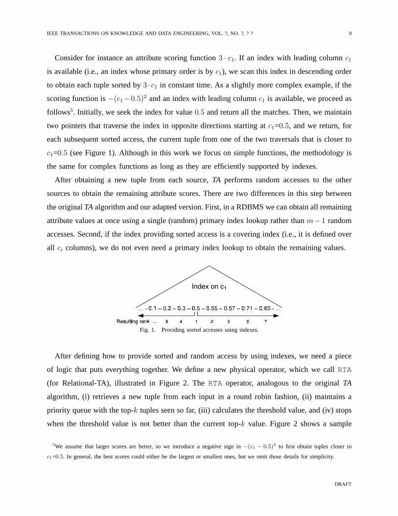
Consider for instance an attribute scoring function3 · c1. If an index with leading columnc1
is available (i.e., an index whose primary order is byc1), we scan this index in descending order
to obtain each tuple sorted by3 · c1 in constant time. As a slightly more complex example, if the
scoring function is−(c1−0.5)2 and an index with leading columnc1 is available, we proceed as
follows5. Initially, we seek the index for value0.5 and return all the matches. Then, we maintain
two pointers that traverse the index in opposite directionsstarting atc1=0.5, and we return, for
each subsequent sorted access, the current tuple from one ofthe two traversals that is closer to
c1=0.5 (see Figure 1). Although in this work we focus on simple functions, the methodology is
the same for complex functions as long as they are efficientlysupported by indexes.
After obtaining a new tuple from each source,TA performs random accesses to the other
sources to obtain the remaining attribute scores. There aretwo differences in this step between
the originalTAalgorithm and our adapted version. First, in a RDBMS we can obtain all remaining
attribute values at once using a single (random) primary index lookup rather thanm−1 random
accesses. Second, if the index providing sorted access is a covering index (i.e., it is defined over
all ci columns), we do not even need a primary index lookup to obtainthe remaining values.
Index on c�� � ��� � ��� � ��� � �� � �� � �� � ��� � ��� � ������ � � � � � ���������� ����Fig. 1. Providing sorted accesses using indexes.
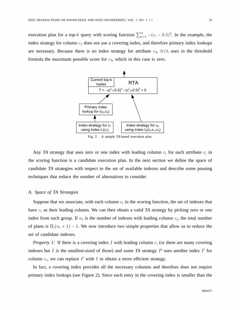
After defining how to provide sorted and random access by using indexes, we need a piece
of logic that puts everything together. We define a new physical operator, which we callRTA
(for Relational-TA), illustrated in Figure 2. TheRTA operator, analogous to the originalTA
algorithm, (i) retrieves a new tuple from each input in a round robin fashion, (ii) maintains a
priority queue with the top-k tuples seen so far, (iii) calculates the threshold value, and (iv) stops
when the threshold value is not better than the current top-k value. Figure 2 shows a sample
5We assume that larger scores are better, so we introduce a negative sign in−(c1 − 0.5)2 to first obtain tuples closer to
c1=0.5. In general, the best scores could either be the largest or smallest ones, but we omit those details for simplicity.
DRAFT
IEEE TRANSACTIONS ON KNOWLEDGE AND DATA ENGINEERING, VOL. ?, NO. ?, ? ? 10
execution plan for a top-k query with scoring function∑3
i=1 −(ci − 0.5)2. In the example, the
index strategy for columnc1 does not use a covering index, and therefore primary index lookups
are necessary. Because there is no index strategy for attribute c3, RTA uses in the threshold
formula the maximum possible score forc3, which in this case is zero.
Index strategy for c1using index I1(c1)
Primary index
lookup for (c2,c3)
Index strategy for c2using index I2(c2,c1,c3)
Current top-k
tuples
T = -(cL1-0.5)
2- (c
L2-0.5)
2+ 0
RTA
Fig. 2. A sampleTA-based execution plan.
Any TA strategy that uses zero or one index with leading columnci for each attributeci in
the scoring function is a candidate execution plan. In the next section we define the space of
candidateTA strategies with respect to the set of available indexes and describe some pruning
techniques that reduce the number of alternatives to consider.
A. Space of TA Strategies
Suppose that we associate, with each columnci in the scoring function, the set of indexes that
haveci as their leading column. We can then obtain a validTA strategy by picking zero or one
index from each group. Ifni is the number of indexes with leading columnci, the total number
of plans isΠi(ni + 1)− 1. We now introduce two simple properties that allow us to reduce the
set of candidate indexes.
Property 1: If there is a covering indexI with leading columnci (or there are many covering
indexes butI is the smallest-sized of those) and someTA strategyP uses another indexI ′ for
columnci, we can replaceI ′ with I to obtain a more efficient strategy.
In fact, a covering index provides all the necessary columnsand therefore does not require
primary index lookups (see Figure 2). Since each entry in thecovering index is smaller than the
DRAFT
IEEE TRANSACTIONS ON KNOWLEDGE AND DATA ENGINEERING, VOL. ?, NO. ?, ? ? 11
corresponding one in the primary index, the number of pages accessed using the covering index
is no larger than the number of pages accessed by a non-covering index and the primary index
lookups put together. Similarly, if many covering indexes are available, the smallest-sized one
accesses the least number of pages. Therefore, the strategythat uses theI is more efficient than
any of the alternatives.
Property 2: Suppose that there is no covering index with leading columnci. If I is the
smallest-sized index with leading columnci and someTA strategyP uses another indexI ′ for
columnci, we can replaceI ′ with I to obtain a more efficient strategy.
In fact, if no covering index is available forci, then any index that handles attributeci
would miss at least one attribute, and therefore would require one (and only one) primary index
lookup to obtain the remaining attribute scores. The smallest-sized index with leading column
ci guarantees that the index traversal is as efficient as possible. In addition, independently of
the index used forci, the subsequent operators (including the primary index lookups) are the
same. Therefore, the smallest-sized index with leading column ci results in the most efficient
execution.
Using both properties, the space of candidateTA strategies is reduced, for each attributeci
in the scoring function, to either zero or the best index forci. We next show that in absence of
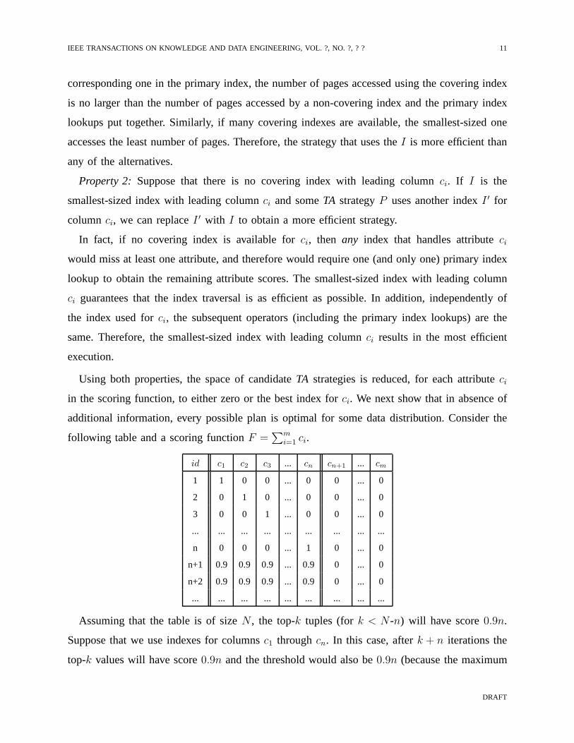
additional information, every possible plan is optimal forsome data distribution. Consider the
following table and a scoring functionF =∑m
i=1 ci.
id c1 c2 c3 ... cn cn+1 ... cm
1 1 0 0 ... 0 0 ... 0
2 0 1 0 ... 0 0 ... 0
3 0 0 1 ... 0 0 ... 0
... ... ... ... ... ... ... ... ...
n 0 0 0 ... 1 0 ... 0
n+1 0.9 0.9 0.9 ... 0.9 0 ... 0
n+2 0.9 0.9 0.9 ... 0.9 0 ... 0
... ... ... ... ... ... ... ... ...
Assuming that the table is of sizeN , the top-k tuples (fork < N-n) will have score0.9n.
Suppose that we use indexes for columnsc1 throughcn. In this case, afterk + n iterations the
top-k values will have score0.9n and the threshold would also be0.9n (because the maximum
DRAFT
IEEE TRANSACTIONS ON KNOWLEDGE AND DATA ENGINEERING, VOL. ?, NO. ?, ? ? 12
score for all columns without indexes is zero). Therefore, after k + n iterations the algorithm
would terminate. Now, if we use indexes over any subset of{c1, c2, . . . , cn}, the threshold value
after any number of iterations beyondn would be0.9n1 + 1(n − n1) for somen1 < n, which
is larger than the current top-k value 0.9n. Therefore, this strategy would require reading all
N tuples from such indexes and would in general be more expensive than the previous one.
Finally, we note that any plan that uses indexes fromcn+1 throughcm will be more expensive
than if those indexes are not used, because they do not reducethe threshold and therefore the
number of iterations remains the same while the number of index sorted accesses increase. In
conclusion, the best possibleTA strategy uses indexes just forc1 throughcn. But those columns
are arbitrary, so for any candidateTA strategy there will be a data distribution for which it is
optimal.
More importantly, depending on the data distribution and available indexes, the best possible
TA strategy might be worse than the scan-based alternative. Infact, consider the table above,
and suppose thatN = n + k. In this case, the strategy that uses all indexesc1 throughcn is still
optimal, but it terminates aftern + k = N iterations (in fact, anyTA strategy terminates after
N iterations for this specific data set). Depending on the available indexes, each iteration may
require a number of random accesses. Therefore, the optimalstrategy would require at least as
many random accesses as objects in the original table. The best TA strategy in this case will
therefore take more time than a simpleScanalternative. For that reason, it is crucial that we
develop a cost model that not only allows us to compare candidateTA strategies, but also help
us decide whether the bestTA strategy is expected to be more efficient than the scan-based
alternative. In the next section we introduce such cost model.
B. Cost Model
Although TA strategies are new to an RDBMS, they are composed of smaller pieces that are
well-known and implemented in current systems. Any execution of TA consists of a series of
sorted accesses (i.e., index traversals), a series of random accesses (i.e., optional primary index
lookups in absence of covering indexes), and some computation to obtain scores, threshold
values, and priority queue maintenance (i.e., scalar computation and portions of thepartial-sort
operator). If a givenTA strategy requiresD iterations to finish (i.e.,D sorted accesses over each
DRAFT
IEEE TRANSACTIONS ON KNOWLEDGE AND DATA ENGINEERING, VOL. ?, NO. ?, ? ? 13
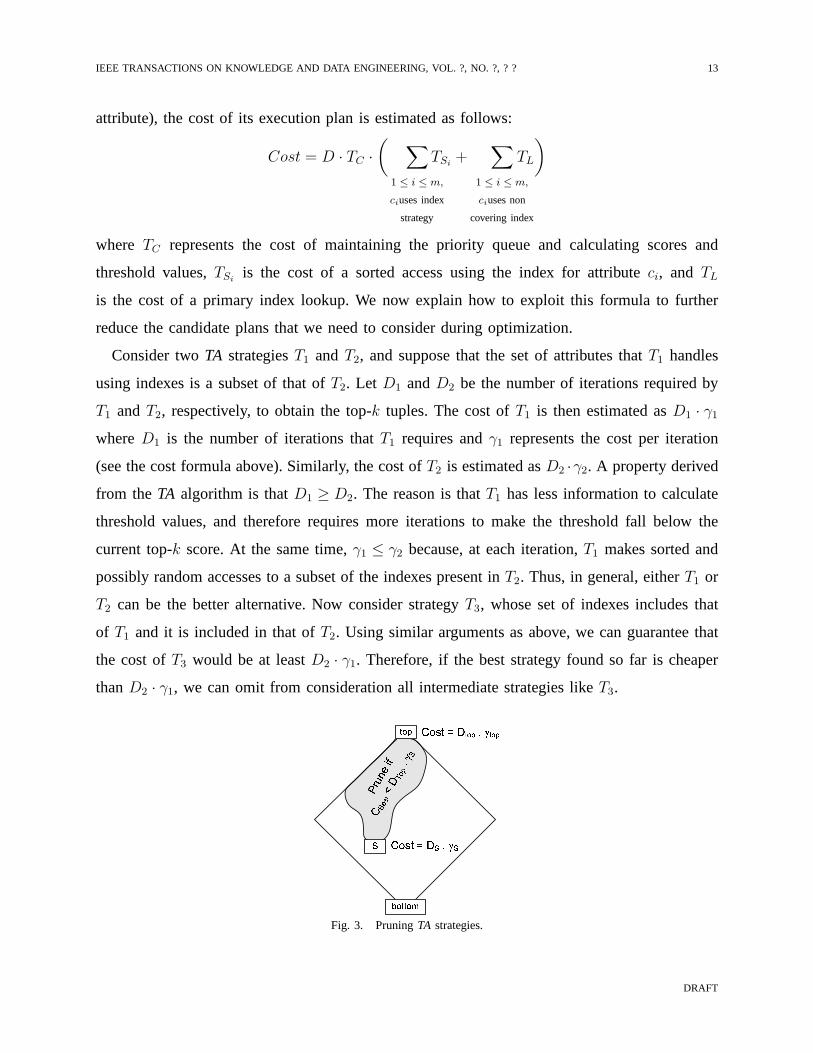
attribute), the cost of its execution plan is estimated as follows:
Cost = D · TC ·
(
∑
1 ≤ i ≤ m,
ciuses index
strategy
TSi+
∑
1 ≤ i ≤ m,
ciuses non
covering index
TL
)
where TC represents the cost of maintaining the priority queue and calculating scores and
threshold values,TSiis the cost of a sorted access using the index for attributeci, and TL
is the cost of a primary index lookup. We now explain how to exploit this formula to further
reduce the candidate plans that we need to consider during optimization.
Consider twoTA strategiesT1 and T2, and suppose that the set of attributes thatT1 handles
using indexes is a subset of that ofT2. Let D1 andD2 be the number of iterations required by
T1 andT2, respectively, to obtain the top-k tuples. The cost ofT1 is then estimated asD1 · γ1
whereD1 is the number of iterations thatT1 requires andγ1 represents the cost per iteration
(see the cost formula above). Similarly, the cost ofT2 is estimated asD2 ·γ2. A property derived
from theTA algorithm is thatD1 ≥ D2. The reason is thatT1 has less information to calculate
threshold values, and therefore requires more iterations to make the threshold fall below the
current top-k score. At the same time,γ1 ≤ γ2 because, at each iteration,T1 makes sorted and
possibly random accesses to a subset of the indexes present in T2. Thus, in general, eitherT1 or
T2 can be the better alternative. Now consider strategyT3, whose set of indexes includes that
of T1 and it is included in that ofT2. Using similar arguments as above, we can guarantee that
the cost ofT3 would be at leastD2 · γ1. Therefore, if the best strategy found so far is cheaper
thanD2 · γ1, we can omit from consideration all intermediate strategies like T3. !"#! !$%
&'() * +,-. / 0,-.&'() * +1 / 0123456789:;<=>?@ABCDE
Fig. 3. PruningTA strategies.
DRAFT
IEEE TRANSACTIONS ON KNOWLEDGE AND DATA ENGINEERING, VOL. ?, NO. ?, ? ? 14
In practice, we can use this property as follows. Figure 3 shows a lattice on the subset of
indexes used byTA strategies. Suppose that we initially evaluate the cost of strategyTop, which
uses indexes for all columns, and obtainDTop as the estimated number of iterations. Assume
that the best strategy found so far has cost equal toCbest. Whenever we consider a new strategy
S, we can calculate the cost per iterationγS. If DTop · γS > Cbest we can safely omit from
consideration allTA strategies that includeS’s indexes.
In the above cost formula, all components can be accurately estimated reusing the cost model
of the database optimizer, except for the number of iterationsD. This value depends on the data
distribution and crucially determines the overall cost ofTA. We now show how to estimate the
expected number of iterationsD for a givenTA strategy.
C. Estimating the Complexity of TA
As explained above, in order to estimate the cost of any givenTA strategy, we need to
approximate the number of iterationsD that such strategy would execute before the threshold
value falls below the current (and therefore final) top-k score. In other words, if we denotesk
the score of the top-k tuple andT (d) the value of the threshold afterd iterations, we need to
estimateD, the minimum value ofd such thatT (d) ≤ sk. We will find D by approximating
the two sides of this inequality. We first approximatesk, the score of the top-k tuple. Then, we
estimate the minimum valued after whichT (d) is expected to fall belowsk.
Let us first assume that we already estimatedsk, the score of the top-k tuple. To approx-
imate the number of iterations after which the threshold value falls belowsk we use single-
column histograms. In fact, an important observation regarding TA is that it manipulates single-
dimensional streams of data returned by the autonomous sources, and therefore exploiting single-
column histograms for the approximation does not implicitly assume independence. Thus, we
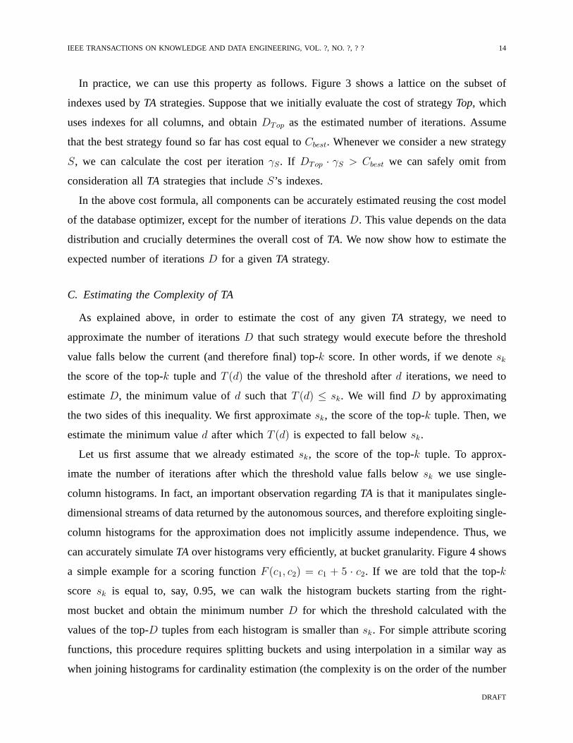
can accurately simulateTA over histograms very efficiently, at bucket granularity. Figure 4 shows
a simple example for a scoring functionF (c1, c2) = c1 + 5 · c2. If we are told that the top-k
score sk is equal to, say, 0.95, we can walk the histogram buckets starting from the right-
most bucket and obtain the minimum numberD for which the threshold calculated with the
values of the top-D tuples from each histogram is smaller thansk. For simple attribute scoring
functions, this procedure requires splitting buckets and using interpolation in a similar way as
when joining histograms for cardinality estimation (the complexity is on the order of the number
DRAFT
IEEE TRANSACTIONS ON KNOWLEDGE AND DATA ENGINEERING, VOL. ?, NO. ?, ? ? 15
v1(d)
d
d
H(c1)
H(c2)
Scoring Function
F(c1,c2) = c1 + 5 c2Threshold(d) ≈ v1(d) + 5 v2(d)
v2(d)
Fig. 4. ApproximatingD using histograms.
of histogram buckets). For complex attribute scoring functions, we use binary search over the
histogram domains to findD, which is also very efficient.
As we will see, estimating the scoresk of the top-k tuple is more complex. The difficulty
resides on the fact that this is a truly multidimensional problem, and therefore relying on
single-dimensional approximations (like traditional histograms) can easily result in excessive
approximation errors. For that reason, we need to use multidimensional data synopses to estimate
sk values. We considered multidimensional histograms and samples as alternative synopses, and
experimentally determined that samples provided the best results. The reason is that multidi-
mensional samples scale better with increasing number of dimensions. In fact, it is known that
multidimensional histograms do not provide accurate estimations beyond five to six attributes
(e.g., see [15], [16]) and therefore we would need to build a large number of at most 5-
dimensional histograms to cover all attribute combinations in wide tables. We note that, unlike
previous work in approximate query processing, our precomputed samples must be very small.
The reason is that these samples are loaded and manipulated as part of query optimization, and
therefore must be roughly of the size of other database statistics. In other words, single-column
projection of the precomputed sample must be roughly as large as a single-column histogram in
the database system. In all our experiments, we use a sample size of 1,000 tuples, independently
of the size of the underlying table.
To estimate the valuesk from the precomputed sample we proceed as follows. We first compute
the score of each tuple in the sample and order the scores by decreasing score value. We then
estimatesk using interpolation. If the original table containsN tuples and the sample containsS
tuples, the probability that the top-rS element in the sample is the top-rN element in the original
DRAFT
IEEE TRANSACTIONS ON KNOWLEDGE AND DATA ENGINEERING, VOL. ?, NO. ?, ? ? 16
data, denotedP (rS is rN ), is given by:
P (rS is rN) =
(
rN−1rS−1
)
·(
N−rN
S−rS
)
(
N
S
)
and therefore, the expected rank in the original table of thetop-rS tuple in the sample, denoted
E(rS), is given by:
E(rS) =∑
i
(
i−1rS−1
)
·(
N−i
S−rS
)
(
N
S
) · i = rS ·N + 1
S + 1
Using this equation, we locate the two consecutive samples in descending order of score that
are expected to cover the top-k element in the original data and interpolate their respective scores
to obtain an approximation ofsk. The estimation algorithm can then be summarized as follows:
1) Using a precomputed small sample, obtain the approximatescoresk of the top-k tuple.
2) Using single-column histograms, obtain the minimum value D that results in a threshold
value belowsk.
3) Evaluate the cost function usingD as the approximation of the number of iterations.
We note that this algorithm can be used for arbitraryTA strategies, by using in step 2 only the
histograms that correspond to columns that are handled using indexes in the query plan (the
remaining columns simulateTA by using the maximum possible score). On the other hand, the
above algorithm presents some problems for the class of top-k queries that we address in this
work. In the next section we explain these obstacles and how we address them.
D. Addressing Smallk Values
Unfortunately, the algorithm of the previous section has animportant drawback in most
interesting query instances. The problem is that only around a thousand tuples are used in
the precomputed sample, and therefore we are always workingon the tails of probability
distributions. For instance, suppose that our data set contains 1 million tuples, and we use a
sample of size 1,000. In this case, the top scoring tuple in the sample is expected to rank at
position 1,000,0011,001
≈ 999 in the original table. This means that for any top-k query withk < 999
(i.e., a very common scenario),sk would likely be smaller than the top tuple in the sample.
In this situation, we would need extrapolate the top-k score. As we show in the experimental
section, this procedure generally results in large approximation errors. In this section we discuss
two complementary approaches to address this issue.
DRAFT
IEEE TRANSACTIONS ON KNOWLEDGE AND DATA ENGINEERING, VOL. ?, NO. ?, ? ? 17
Interpolating Iterations rather than Object Scores
We next propose an alternative approximation mechanism that works in the space of iterations
of TA rather than on the space of object scores. We first obtain the top-k′ scores from the
precomputed sample wherek′ is a small constant number (we usek′ = 10 in our experiments).
If the original table containsN tuples and the sample size isS, the top-k′ scores in the sample
are expected to rank in the original table at positionsi · N+1S+1
for i = 1..10. We then calculate
as before the approximated number of iterations for each such score and obtain a set of pairs
{(i · N+1S+1
, expected iterations fori · N+1S+1
), i = 1..10}. Finally, we fit the best curve that assigns
expected number of iterations to obtain top-K values for arbitrary values ofK, and evaluate this
function atK = k. We use the obtained value as the estimated number of iterations to obtain
the top-k elements. The revised algorithm can be summarized as follows:
1) Using a precomputed small sample, obtain the top-10 scores that are expected to rank in
the original data at positionsN+1S+1
, . . . , 10·(N+1)S+1
.
2) Using single-column histograms, obtain the expected number of iterations for each score.
3) Find the best curve that approximate the “number of iterations” function and evaluate it
in k obtainingD.
4) Evaluate the cost function usingD as an approximation for the number of iterations.
An important decision is which model function to use to approximate number of iterations
for arbitrary values ofk. The simplest approach is to use linear regression, but manyothers
are possible. After an extensive experimental evaluation,we decided to use a power function
D(k) = a ·eb·k wherea andb are parameters that minimize the square root error6. Of course, this
is just an approximation as the true underlying function depends on the data distribution and in
general can have any (monotonically increasing) behavior.However, we found that power laws
resulted in the best overall accuracy for a wide class of datadistributions and scoring functions
(see Section V for some examples that validate our choice of model functions).
6Note that [13] introduces an earlier algorithm to obtain top-k answers with a probabilistic access cost that follows a power
law in terms ofk.
DRAFT
IEEE TRANSACTIONS ON KNOWLEDGE AND DATA ENGINEERING, VOL. ?, NO. ?, ? ? 18
Using a Safety Factor for Large Rank Variance
A second difficulty that our techniques face arises from the limited sample size. As we
explained earlier, the expected rank in the data distribution of thei-th highest ranked element
in the sample isi · N+1S+1
. We now briefly analyze how accurate that estimation is for the special
case ofi=1 (i.e., how close toN+1S+1
in the original data set is the rank of the top object in the
sample). The variance of the rank in the original table of thetop tuple in the sample, denoted
V (1S), is given by:
V (1S) =∑
i
(
N−i
S−1
)
(
N
S
) ·(N + 1
S + 1− i
)2
=S(N + 1)(N2 − NS − 3N + S2 + 2)
(S + 1)2(S + 2)(N − S + 1)
which is approximately(
N+1S+1
)2if N ≫ S. In other words, the standard deviation of the rank
in the original relation of the top object in the sample is as large as the expected rank itself.
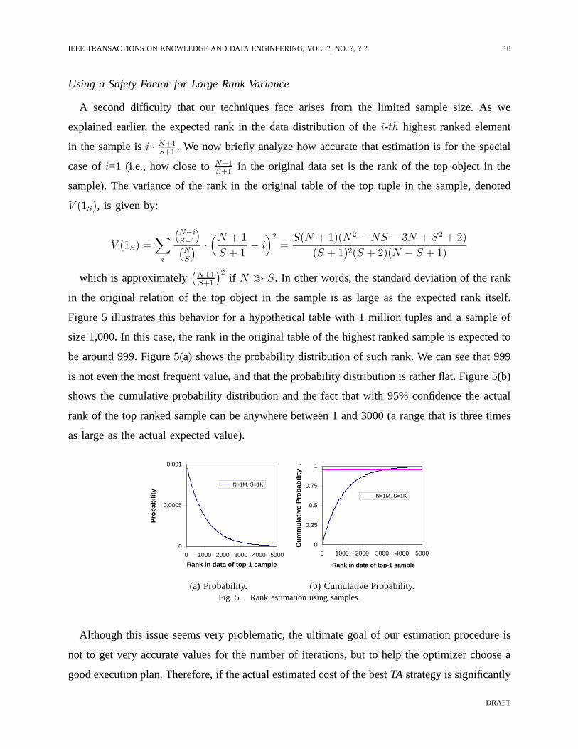
Figure 5 illustrates this behavior for a hypothetical tablewith 1 million tuples and a sample of
size 1,000. In this case, the rank in the original table of thehighest ranked sample is expected to
be around 999. Figure 5(a) shows the probability distribution of such rank. We can see that 999
is not even the most frequent value, and that the probabilitydistribution is rather flat. Figure 5(b)
shows the cumulative probability distribution and the factthat with 95% confidence the actual
rank of the top ranked sample can be anywhere between 1 and 3000 (a range that is three times
as large as the actual expected value).
0
0.0005
0.001
0 1000 2000 3000 4000 5000
Rank in data of top-1 sample
Pro
bab
ility
N=1M, S=1K
0
0.25
0.5
0.75
1
0 1000 2000 3000 4000 5000
Rank in data of top-1 sample
Cu
mm
ula
tive
Pro
bab
ility
.
N=1M, S=1K
(a) Probability. (b) Cumulative Probability.Fig. 5. Rank estimation using samples.
Although this issue seems very problematic, the ultimate goal of our estimation procedure is
not to get very accurate values for the number of iterations,but to help the optimizer choose a
good execution plan. Therefore, if the actual estimated cost of the bestTA strategy is significantly
DRAFT
IEEE TRANSACTIONS ON KNOWLEDGE AND DATA ENGINEERING, VOL. ?, NO. ?, ? ? 19
larger or smaller than that of the scan-based alternative, moderate variations in the estimation
of cost will not change the optimal plan from being chosen. When the two numbers are close,
though, there is a larger chance that errors in estimation will propagate to the selection of plans.
We examine these issues in the experimental section.
We use an additional small “safety” factor as follows. Recall that the procedure to estimate
the cost of anyTA strategy uses some approximations that are intrinsically not very accurate. On
the other hand, the cost estimation for a scan alternative can be estimated very accurately. As
a conservative measure, we only choose aTA strategy if it is cheaper thanα times the cost of
an alternative scan, where0 < α ≤ 1 (we useα = 0.5 in our experiments, but this number can
in general reflect the degree of confidence that we require before executing aTA strategy). We
choose aTA strategy only if we are confident enough that it will be cheaper than the scan-based
alternative. In doing so we might choose the scan-based alternative even though aTA strategy
was indeed the optimal plan, but this is an expected consequence of our conservative approach.
We analyze this tradeoff experimentally in Section V.
IV. EXTENSIONS
In this section we discuss some extensions that can be easilyincorporated to our model.
A. Handling Filter Predicates
In the previous section we assumed that there was no filter predicate restricting the set of
tuples that qualify to be part of the answer. We now describe how we can relax that restriction.
Consider the general query:
SELECT TOP(k) c1, ..., cm
FROM R
WHERE P
ORDER BY F(s1(c1), ..., sm(cm)) DESC
whereP is an arbitrary predicate over the columns ofR. We now discuss how we can evaluate
such queries and then how we can estimate their execution cost.
1) Execution Alternatives:A straightforward extension ofTA to handle arbitrary filter pred-
icates is as follows. Recall from Figure 2 the main components of a typicalTA strategy. The
idea is to add a small piece of logic in theRTA operator, which evaluates predicateP before
DRAFT
IEEE TRANSACTIONS ON KNOWLEDGE AND DATA ENGINEERING, VOL. ?, NO. ?, ? ? 20
considering the addition of the current object to the set of top-k tuples. If the current tuple
does not satisfyP, it is dropped from consideration. The calculation of the threshold, however,
considers all tuples whether they satisfyP or not. This execution strategy is feasible ifRTA
receives input tuples that additionally reference all the columns required to evaluateP. If the
current tuple is obtained from an index strategy followed bya primary index lookup, then all
relevant columns are already present. Otherwise, if a covering index is used, we need to perform
an additional index lookup to obtain the remaining columns.Of course, if the covering index
additionally contains all columns referenced byP, then there is no need to do any primary index
lookup. All the pruning considerations are similar to the original case discussed in Section III-B.
If the predicateP satisfies certain properties, there is a different alternative that might be more
efficient, especially ifP is selective. Consider the following query:
SELECT TOP(10) a, b, c
FROM R
WHERE d=10
ORDER BY a+b+c DESC
and suppose that an index on columnd is available. In that case, we can push the selection
condition into the order by clause and transform the query above as follows:
SELECT TOP(k) a, b, c
FROM R
ORDER BY a+b+c+
0 if d=10
−∞ otherwiseDESC
It is fairly simple to see that, if there are at leastk tuples for whichd=10 both queries are
equivalent (otherwise, we need to discard from the latter query all the tuples with score equal
to −∞). In this case, we reduced a query with a filter predicate to anequivalent one that does
not have it. Also, the index on columnd can be used to return all tuples that satisfy the filter
predicate before any tuple that does not satisfy it7. In general, we can use this alternativeTA
strategy by pushing to the scoring function all predicates that can be efficiently retrieved using
indexes.
7After the first tuple that not satisfyingP is returned, the threshold value drops below the current top-k score and execution
terminates.
DRAFT
IEEE TRANSACTIONS ON KNOWLEDGE AND DATA ENGINEERING, VOL. ?, NO. ?, ? ? 21
2) Cost Estimation:A key observation to estimate the cost of the extended strategies discussed
above is that introducing filter predicates does not changeTA’s early termination condition, which
is “stop after the threshold falls below the score of the current (and final) top-k object”. Therefore,
the procedure explained in Section III-B can also be used in this scenario. The difference is that
initially we need to apply predicateP to the precomputed sample so that we only consider
tuples that satisfy the filter predicate. Note, however, that the accuracy of this method will
diminish since the effective sample that we use for estimation is smaller than the original one.
For instance, a very selective predicate might filter out allbut five tuples in the original sample
S. The actual number of tuples in the resulting sampleS ′ would therefore be too small, which
makes our techniques more difficult to apply (e.g., recall from Section III-D that we need at
least ten elements in the sample to fit the best power law that determines the expected cost of
a TA strategy).
B. Other Enhancements
There are other enhancements to the main algorithm that can speed up the overall execution
of a top-k query. For instance,TA uses bounded buffers and only stores the current top-k objects
in a priority queue. While this is important to guarantee that the algorithm will not run out of
memory during its execution, some objects might be looked upin the primary index multiple
times if they are not part of the top-k objects (once each time an object is retrieved from a
source). We can trade space for time by keeping a hash table ofall objects already seen. If we
retrieve an object using sorted access and it is already in the hash table, we do not process it
again (saving a primary index lookup).
An optimization studied in the literature is to relax the requirement that sorted accesses are
done in a round-robin fashion [14]. In general, we can accesseach source at different rates, and
retrieve tuples more often from those sources that contribute more to decreasing the threshold
value. Conversely, if the score distribution of an attribute is close to uniform, we can decrease
the rate at which we request new tuples from that source. It isfairly straightforward to show
that a strategy that performs sorted accesses at different rates can be better than any alternative
strategy that proceeds in lockstep. It is interesting to note that for fixed, but different access rates
to the sources, the estimation technique of Section III-B that uses single-column histograms
can be applied with almost no changes. In this case, we would obtain the minimum values
DRAFT

IEEE TRANSACTIONS ON KNOWLEDGE AND DATA ENGINEERING, VOL. ?, NO. ?, ? ? 22
{D1, . . . , Dm} for which the threshold value calculated with the top-Di value for each attribute
ci is expected to fall below the top-k score.
Finally, there are opportunities to further avoid primary index lookups. Consider a top-k query
over attributesa, b, and c, and suppose that we use a composite non-covering index on(a, b)
to process attributea. For each tuple retrieved from the index, we can first assume that the
value of c is as large as possible. If the resulting score calculated inthat way is still smaller
than the current top-k score, we can discard the tuple without performing a primaryindex
lookup. Although this idea is at first glance straightforward, it carries important implications for
optimization. Specifically, our pruning techniques of Section III-A need to be refined to work
in this scenario. For instance, if indexes over both(a) and(a, b) are available for a top-k query
over attributea, b, and c, our pruning techniques would not consider(a, b) (see Property 2),
which might be the best alternative when this optimization is used.
Implementing these enhancements and providing suitable extensions to the cost model is part
of future work.
V. EXPERIMENTAL EVALUATION
We next report an extensive experimental evaluation of our techniques, which we implemented
in Microsoft SQL Server. We note that, aside from our own extensions, we did not use vendor-
specific features in our experiments. We therefore believe that our results would be directly
applicable to other implementations of SQL that support multi-column indexes. Below we detail
the data sets, techniques, and metrics used for the experiments of this section.
Data Sets: We use both synthetic and real data sets for the experiments.The real data set
we consider isCovType [17], a 55-dimensional data set used for predicting forest cover types
from cartographic variables. Specifically, we consider thefollowing quantitative attributes for our
experiments: elevation, aspect, slope, horizontal and vertical distances to hydrology, horizontal
distances to roadways and fire points, and hill shades at different times of the day. The cardinality
CovType is around 545,000 tuples.
To evaluate specific aspects of our techniques we also generated a synthetic data distribution
with 1 million tuples and 14 attributes with different distributions and degrees of correlation.
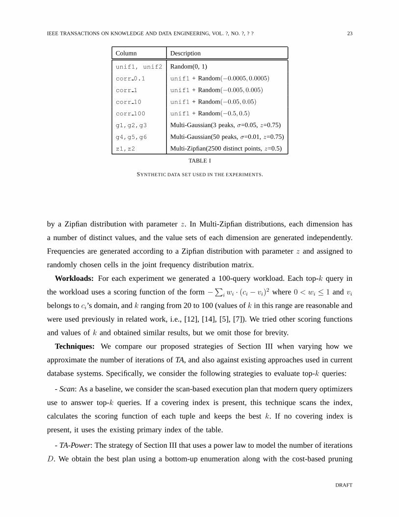
Table I described the attributes of the synthetic database.Multi-Gaussian distributions consist of
a number of overlapping gaussian bells, where the number of tuples on each bell is regulated
DRAFT
IEEE TRANSACTIONS ON KNOWLEDGE AND DATA ENGINEERING, VOL. ?, NO. ?, ? ? 23
Column Description
unif1, unif2 Random(0, 1)
corr 0.1 unif1 + Random(−0.0005, 0.0005)
corr 1 unif1 + Random(−0.005, 0.005)
corr 10 unif1 + Random(−0.05, 0.05)
corr 100 unif1 + Random(−0.5, 0.5)
g1,g2,g3 Multi-Gaussian(3 peaks,σ=0.05,z=0.75)
g4,g5,g6 Multi-Gaussian(50 peaks,σ=0.01,z=0.75)
z1,z2 Multi-Zipfian(2500 distinct points,z=0.5)
TABLE I
SYNTHETIC DATA SET USED IN THE EXPERIMENTS.
by a Zipfian distribution with parameterz. In Multi-Zipfian distributions, each dimension has
a number of distinct values, and the value sets of each dimension are generated independently.
Frequencies are generated according to a Zipfian distribution with parameterz and assigned to
randomly chosen cells in the joint frequency distribution matrix.
Workloads: For each experiment we generated a 100-query workload. Eachtop-k query in
the workload uses a scoring function of the form−∑
i wi · (ci − vi)2 where0 < wi ≤ 1 andvi
belongs toci’s domain, andk ranging from 20 to 100 (values ofk in this range are reasonable and
were used previously in related work, i.e., [12], [14], [5],[7]). We tried other scoring functions
and values ofk and obtained similar results, but we omit those for brevity.
Techniques: We compare our proposed strategies of Section III when varying how we
approximate the number of iterations ofTA, and also against existing approaches used in current
database systems. Specifically, we consider the following strategies to evaluate top-k queries:
- Scan: As a baseline, we consider the scan-based execution plan that modern query optimizers
use to answer top-k queries. If a covering index is present, this technique scans the index,
calculates the scoring function of each tuple and keeps the best k. If no covering index is
present, it uses the existing primary index of the table.
- TA-Power: The strategy of Section III that uses a power law to model thenumber of iterations
D. We obtain the best plan using a bottom-up enumeration alongwith the cost-based pruning
DRAFT
IEEE TRANSACTIONS ON KNOWLEDGE AND DATA ENGINEERING, VOL. ?, NO. ?, ? ? 24
technique of Section III-B.
- TA-Power-Greedy: This strategy uses the same cost model asTA-Power, but in addition
to the cost-based pruning we use a greedy strategy to enumerate alternative plans. The greedy
technique is similar to the one used to enumerate index intersection plans in traditional database
systems.
- TA-Linear: A variant of TA-Power that uses linear regression instead of power laws to
estimate the number of iterations. We include this technique to illustrate the improvement in
accuracy obtained by using power laws.
- TA-Score: This strategy does not use the ideas of Section III-D to handle small k values.
Instead, whenk is smaller thanN+1S+1
for a table withN tuples and a sample of sizeS, we
extrapolatesk, the top-k score as follows. For a scoring functionF (c1, . . . , cm) we first obtain
the maximum possible score of any tuple, denotedsmax, asF (vmax1 , . . . , vmax
m ), wherevmaxi is
the maximum possible value for the attribute score functionof attributeci. Suppose thats1 is
the top-score from any tuple in the precomputed sample. We know that there areN+1S+1
expected
tuples with scores betweens1 and smax. We then approximate the top-k scoresk assuming
uniformity as s1 + (smax − s1) · (k − 1)/(N+1S+1
− 1).
For all the sample-based techniques we use a precomputed 1000-tuple sample.
Metrics: We report experimental results using these metrics:
- AbsoluteD Error. When comparing different cost models, we use the absoluteD error
metric, calculated as follows. For a given technique and query q in the workload, we consider
all possibleTA strategies that are feasible according to the available indexes. For each such
strategys, we estimate the unknown variableD in the cost equation, denotedDq,sest and we also
inspect the data to obtain the exact number of iterationsDq,sact. For a given queryq that admits
TA strategiess1, . . . , sn we calculate the absoluteD error as follows:
1
n
∑
si
∣
∣Dq,si
est − Dq,si
act
∣
∣
The absoluteD error of a workloadW is the average absoluteD error for all queries inW ,
and intuitively represents the accuracy of competing models to approximate the execution cost
of TA strategies.
DRAFT
IEEE TRANSACTIONS ON KNOWLEDGE AND DATA ENGINEERING, VOL. ?, NO. ?, ? ? 25
- Estimated Execution Time.After we establish thatTA-Powerresults in the most accurate
cost estimation among the differentTA techniques, we conduct an experimental evaluation of its
expected performance. For that purpose, we use the following metrics:
- Scan-Time:Expected execution time ofScan, which is the default execution plan in absence
of TA strategies.
- Opt-Time:Expected execution time taken by the optimal strategy when all information is
available. To obtain this value, we inspect the data distribution and obtain the actual number of
iterations required by eachTA strategy. We then calculate the expected cost of eachTA alternative
assuming perfect information and select the most efficient plan among all theTA strategies and
Scan. Opt-Timerepresents the expected time taken by the best possibleTA or Scanalternative
when all cost decisions are perfectly accurate, and it is an upper bound of the improvement that
we can obtain by addingTA strategies to a database system.
- TA-Time:Expected time taken by the best plan chosen by the optimizer (eitherScanor the
bestTA strategy) when usingTA-Powerto estimate the cost ofTA alternatives. To obtain this
value, we calculate the expected cost of eachTA strategy usingTA-Powerand pick the best
plan among theTA strategies andScan. Then, we re-evaluate the cost of such best alternative
(if it is a TA strategy) with the true value ofD obtained by inspecting the data. In other words,
TA-Timeis the expected cost using accurate information of the best execution plan chosen using
TA-Power.
We note that in our experiments we measure expected execution cost (as returned by the query
optimizer) rather than actual execution times. We believe that in the context of this work this is
a better alternative. In fact, after we estimate the number of iterationsD for a givenTA strategy
as shown in Section III-B, our cost model is handled entirelyby the optimizer itself. The cost
model in the optimizer, however, sometimes results in slight inaccuracies with respect to actual
execution times (e.g., sometimes the optimizer might cost asequential scan slightly cheaper than
an index intersection plan when the opposite is actually true). To evaluate our algorithms we
assume that the optimizer has a precise model of execution cost, and use its output as a measure
of query performance. This way we avoid adding another indirection layer that might ultimately
DRAFT
IEEE TRANSACTIONS ON KNOWLEDGE AND DATA ENGINEERING, VOL. ?, NO. ?, ? ? 26
bias our conclusions8.
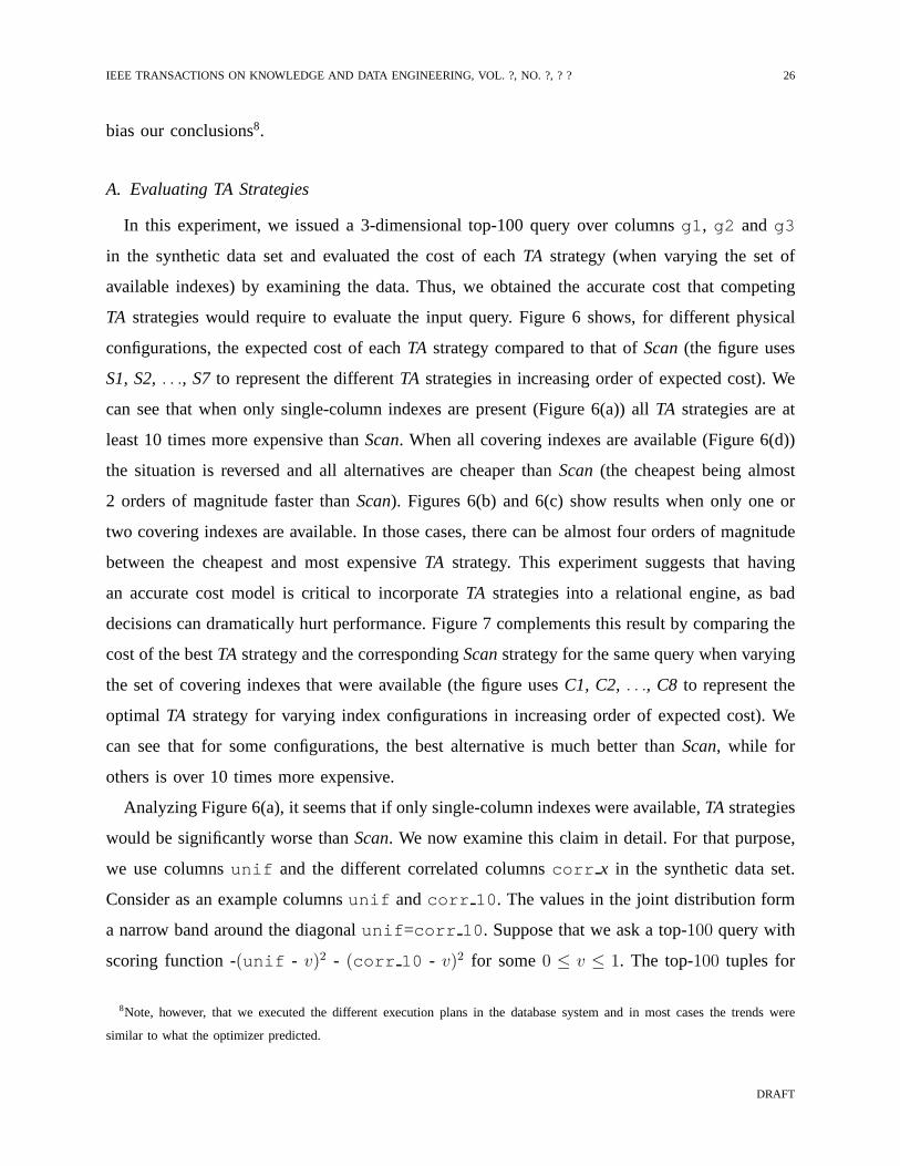
A. Evaluating TA Strategies
In this experiment, we issued a 3-dimensional top-100 queryover columnsg1, g2 andg3
in the synthetic data set and evaluated the cost of eachTA strategy (when varying the set of
available indexes) by examining the data. Thus, we obtainedthe accurate cost that competing
TA strategies would require to evaluate the input query. Figure 6 shows, for different physical
configurations, the expected cost of eachTA strategy compared to that ofScan(the figure uses
S1, S2,. . ., S7to represent the differentTA strategies in increasing order of expected cost). We
can see that when only single-column indexes are present (Figure 6(a)) allTA strategies are at
least 10 times more expensive thanScan. When all covering indexes are available (Figure 6(d))
the situation is reversed and all alternatives are cheaper than Scan(the cheapest being almost
2 orders of magnitude faster thanScan). Figures 6(b) and 6(c) show results when only one or
two covering indexes are available. In those cases, there can be almost four orders of magnitude
between the cheapest and most expensiveTA strategy. This experiment suggests that having
an accurate cost model is critical to incorporateTA strategies into a relational engine, as bad
decisions can dramatically hurt performance. Figure 7 complements this result by comparing the
cost of the bestTA strategy and the correspondingScanstrategy for the same query when varying
the set of covering indexes that were available (the figure usesC1, C2,. . ., C8 to represent the
optimal TA strategy for varying index configurations in increasing order of expected cost). We
can see that for some configurations, the best alternative ismuch better thanScan, while for
others is over 10 times more expensive.
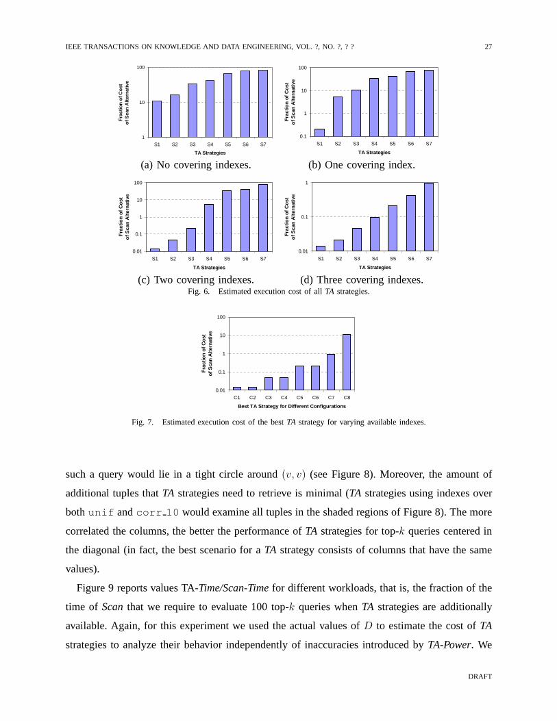
Analyzing Figure 6(a), it seems that if only single-column indexes were available,TA strategies
would be significantly worse thanScan. We now examine this claim in detail. For that purpose,
we use columnsunif and the different correlated columnscorr x in the synthetic data set.
Consider as an example columnsunif andcorr 10. The values in the joint distribution form
a narrow band around the diagonalunif=corr 10. Suppose that we ask a top-100 query with
scoring function -(unif - v)2 - (corr 10 - v)2 for some0 ≤ v ≤ 1. The top-100 tuples for
8Note, however, that we executed the different execution plans in the database system and in most cases the trends were
similar to what the optimizer predicted.
DRAFT
IEEE TRANSACTIONS ON KNOWLEDGE AND DATA ENGINEERING, VOL. ?, NO. ?, ? ? 27
1
10
100
S1 S2 S3 S4 S5 S6 S7
TA Strategies
Fra
ctio
n o
f C
ost
of
Sca
n A
lter
nat
ive
0.1
1
10
100
S1 S2 S3 S4 S5 S6 S7
TA Strategies
Fra
ctio
n o
f C
ost
of
Sca
n A
lter
nat
ive
(a) No covering indexes. (b) One covering index.
0.01
0.1
1
10
100
S1 S2 S3 S4 S5 S6 S7
TA Strategies
Fra
ctio
n o
f C
ost
of
Sca
n A
lter
nat
ive
0.01
0.1
1
S1 S2 S3 S4 S5 S6 S7
TA Strategies
Fra
ctio
n o
f C
ost
of
Sca
n A
lter
nat
ive
(c) Two covering indexes. (d) Three covering indexes.Fig. 6. Estimated execution cost of allTA strategies.
0.01
0.1
1
10
100
C1 C2 C3 C4 C5 C6 C7 C8
Best TA Strategy for Different Configurations
Fra
ctio
n o
f C
ost
of
Sca
n A
lter
nat
ive
Fig. 7. Estimated execution cost of the bestTA strategy for varying available indexes.
such a query would lie in a tight circle around(v, v) (see Figure 8). Moreover, the amount of
additional tuples thatTA strategies need to retrieve is minimal (TA strategies using indexes over
bothunif andcorr 10 would examine all tuples in the shaded regions of Figure 8). The more
correlated the columns, the better the performance ofTA strategies for top-k queries centered in
the diagonal (in fact, the best scenario for aTA strategy consists of columns that have the same
values).
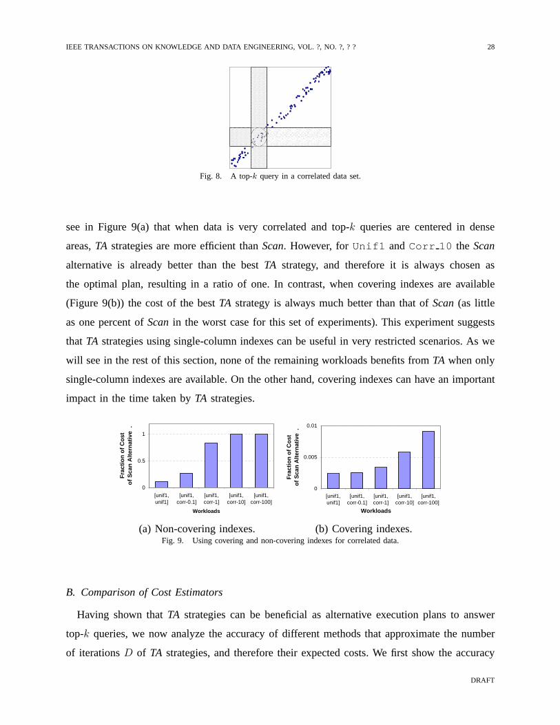
Figure 9 reports values TA-Time/Scan-Timefor different workloads, that is, the fraction of the
time of Scanthat we require to evaluate 100 top-k queries whenTA strategies are additionally
available. Again, for this experiment we used the actual values ofD to estimate the cost ofTA
strategies to analyze their behavior independently of inaccuracies introduced byTA-Power. We
DRAFT
IEEE TRANSACTIONS ON KNOWLEDGE AND DATA ENGINEERING, VOL. ?, NO. ?, ? ? 28
Fig. 8. A top-k query in a correlated data set.
see in Figure 9(a) that when data is very correlated and top-k queries are centered in dense
areas,TA strategies are more efficient thanScan. However, forUnif1 andCorr 10 the Scan
alternative is already better than the bestTA strategy, and therefore it is always chosen as
the optimal plan, resulting in a ratio of one. In contrast, when covering indexes are available
(Figure 9(b)) the cost of the bestTA strategy is always much better than that ofScan(as little
as one percent ofScanin the worst case for this set of experiments). This experiment suggests
that TA strategies using single-column indexes can be useful in very restricted scenarios. As we
will see in the rest of this section, none of the remaining workloads benefits fromTA when only
single-column indexes are available. On the other hand, covering indexes can have an important
impact in the time taken byTA strategies.
0
0.5
1
[unif1,unif1]
[unif1,corr-0.1]
[unif1,corr-1]
[unif1,corr-10]
[unif1,corr-100]
Workloads
Fra
ctio
n o
f C
ost
of
Sca
n A
lter
nat
ive
.
0
0.005
0.01
[unif1,unif1]
[unif1,corr-0.1]
[unif1,corr-1]
[unif1,corr-10]
[unif1,corr-100]
Workloads
Fra
ctio
n o
f C
ost
of
Sca
n A
lter
nat
ive
.
(a) Non-covering indexes. (b) Covering indexes.Fig. 9. Using covering and non-covering indexes for correlated data.
B. Comparison of Cost Estimators
Having shown thatTA strategies can be beneficial as alternative execution plansto answer
top-k queries, we now analyze the accuracy of different methods that approximate the number
of iterationsD of TA strategies, and therefore their expected costs. We first show the accuracy
DRAFT
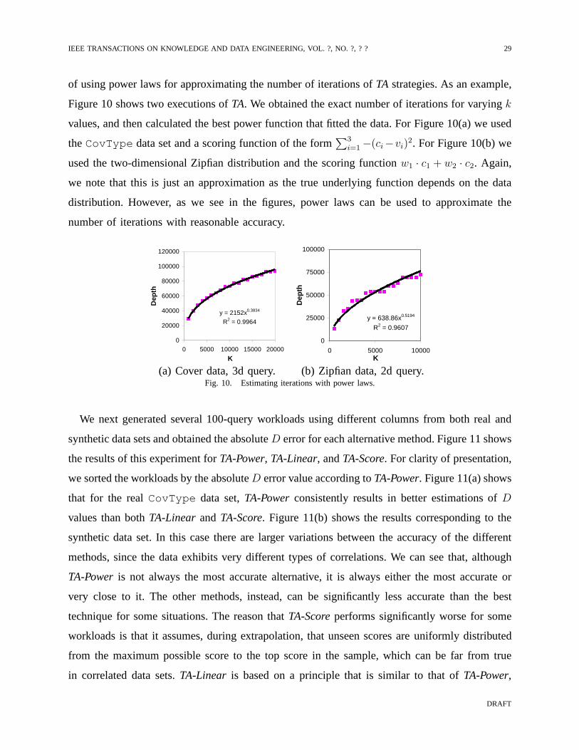
IEEE TRANSACTIONS ON KNOWLEDGE AND DATA ENGINEERING, VOL. ?, NO. ?, ? ? 29
of using power laws for approximating the number of iterations ofTA strategies. As an example,
Figure 10 shows two executions ofTA. We obtained the exact number of iterations for varyingk
values, and then calculated the best power function that fitted the data. For Figure 10(a) we used
theCovType data set and a scoring function of the form∑3
i=1 −(ci−vi)2. For Figure 10(b) we
used the two-dimensional Zipfian distribution and the scoring functionw1 · c1 + w2 · c2. Again,
we note that this is just an approximation as the true underlying function depends on the data
distribution. However, as we see in the figures, power laws can be used to approximate the
number of iterations with reasonable accuracy.
y = 2152x0.3834
R2 = 0.9964
0
20000
40000
60000
80000
100000
120000
0 5000 10000 15000 20000
K
Dep
th
y = 638.86x0.5194
R2 = 0.9607
0
25000
50000
75000
100000
0 5000 10000K
Dep
th
(a) Cover data, 3d query. (b) Zipfian data, 2d query.Fig. 10. Estimating iterations with power laws.
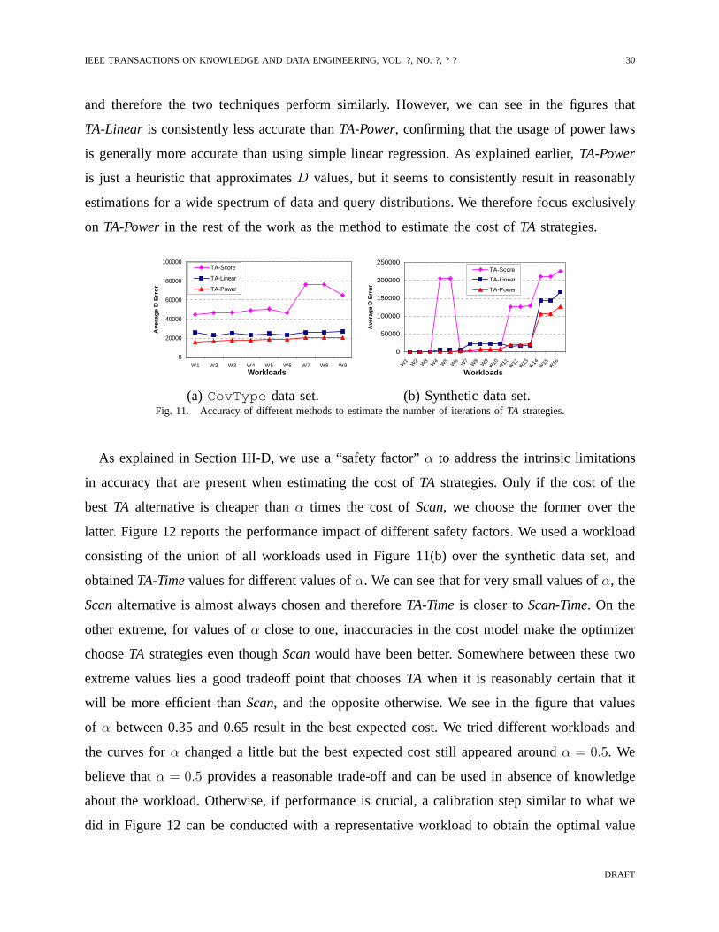
We next generated several 100-query workloads using different columns from both real and
synthetic data sets and obtained the absoluteD error for each alternative method. Figure 11 shows
the results of this experiment forTA-Power, TA-Linear, andTA-Score. For clarity of presentation,
we sorted the workloads by the absoluteD error value according toTA-Power. Figure 11(a) shows
that for the realCovType data set,TA-Powerconsistently results in better estimations ofD
values than bothTA-Linear and TA-Score. Figure 11(b) shows the results corresponding to the
synthetic data set. In this case there are larger variationsbetween the accuracy of the different
methods, since the data exhibits very different types of correlations. We can see that, although
TA-Power is not always the most accurate alternative, it is always either the most accurate or
very close to it. The other methods, instead, can be significantly less accurate than the best
technique for some situations. The reason thatTA-Scoreperforms significantly worse for some
workloads is that it assumes, during extrapolation, that unseen scores are uniformly distributed
from the maximum possible score to the top score in the sample, which can be far from true
in correlated data sets.TA-Linear is based on a principle that is similar to that ofTA-Power,
DRAFT
IEEE TRANSACTIONS ON KNOWLEDGE AND DATA ENGINEERING, VOL. ?, NO. ?, ? ? 30
and therefore the two techniques perform similarly. However, we can see in the figures that
TA-Linear is consistently less accurate thanTA-Power, confirming that the usage of power laws
is generally more accurate than using simple linear regression. As explained earlier,TA-Power
is just a heuristic that approximatesD values, but it seems to consistently result in reasonably
estimations for a wide spectrum of data and query distributions. We therefore focus exclusively
on TA-Powerin the rest of the work as the method to estimate the cost ofTA strategies.
0
20000
40000
60000
80000
100000
W1 W2 W3 W4 W5 W6 W7 W8 W9Workloads
Ave
rag
e D
Err
or
TA-Score
TA-Linear
TA-Power
0
50000
100000
150000
200000
250000
W1
W2
W3
W4
W5
W6
W7
W8
W9
W10
W11
W12
W13
W14
W15
W16
WorkloadsA
vera
ge D
Err
or
TA-Score
TA-Linear
TA-Power
(a) CovType data set. (b) Synthetic data set.Fig. 11. Accuracy of different methods to estimate the number of iterations ofTA strategies.
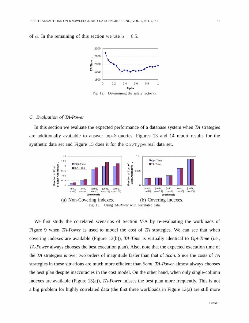
As explained in Section III-D, we use a “safety factor”α to address the intrinsic limitations
in accuracy that are present when estimating the cost ofTA strategies. Only if the cost of the
best TA alternative is cheaper thanα times the cost ofScan, we choose the former over the
latter. Figure 12 reports the performance impact of different safety factors. We used a workload
consisting of the union of all workloads used in Figure 11(b)over the synthetic data set, and
obtainedTA-Timevalues for different values ofα. We can see that for very small values ofα, the
Scanalternative is almost always chosen and thereforeTA-Timeis closer toScan-Time. On the
other extreme, for values ofα close to one, inaccuracies in the cost model make the optimizer
chooseTA strategies even thoughScanwould have been better. Somewhere between these two
extreme values lies a good tradeoff point that choosesTA when it is reasonably certain that it
will be more efficient thanScan, and the opposite otherwise. We see in the figure that values
of α between 0.35 and 0.65 result in the best expected cost. We tried different workloads and
the curves forα changed a little but the best expected cost still appeared aroundα = 0.5. We
believe thatα = 0.5 provides a reasonable trade-off and can be used in absence ofknowledge
about the workload. Otherwise, if performance is crucial, acalibration step similar to what we
did in Figure 12 can be conducted with a representative workload to obtain the optimal value
DRAFT
IEEE TRANSACTIONS ON KNOWLEDGE AND DATA ENGINEERING, VOL. ?, NO. ?, ? ? 31
of α. In the remaining of this section we useα = 0.5.
1800
1900
2000
2100
2200
0 0.2 0.4 0.6 0.8 1
AlphaT
A-T
ime
.Fig. 12. Determining the safety factorα.
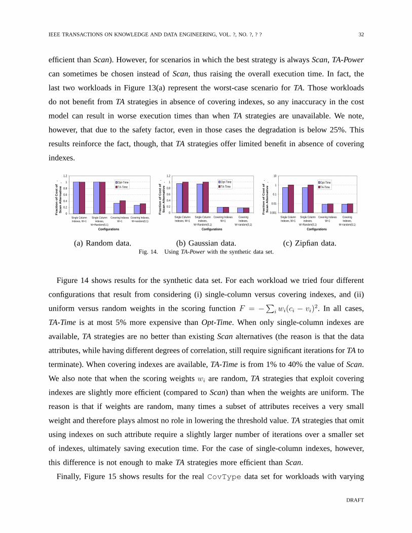
C. Evaluation of TA-Power
In this section we evaluate the expected performance of a database system whenTA strategies
are additionally available to answer top-k queries. Figures 13 and 14 report results for the
synthetic data set and Figure 15 does it for theCovType real data set.
0
0.25
0.5
0.75
1
1.25
1.5
[unif1,unif1]
[unif1,corr-0.1]
[unif1,corr-1]
[unif1,corr-10]
[unif1,corr-100]
Workloads
Frac
tion
of C
ost
.of
Sca
n A
ltern
ativ
e . Opt-Time
TA-Time
0
0.005
0.01
[unif1,unif1]
[unif1,corr-0.1]
[unif1,corr-1]
[unif1,corr-10]
[unif1,corr-100]
Workloads
Frac
tion
of C
ost o
f .
Sca
n A
ltern
ativ
e .
Opt-Time
TA-Time
(a) Non-Covering indexes. (b) Covering indexes.Fig. 13. UsingTA-Powerwith correlated data.
We first study the correlated scenarios of Section V-A by re-evaluating the workloads of
Figure 9 whenTA-Power is used to model the cost ofTA strategies. We can see that when
covering indexes are available (Figure 13(b)),TA-Time is virtually identical toOpt-Time(i.e.,
TA-Poweralways chooses the best execution plan). Also, note that theexpected execution time of
the TA strategies is over two orders of magnitude faster than that of Scan. Since the costs ofTA
strategies in these situations are much more efficient thanScan, TA-Poweralmost always chooses
the best plan despite inaccuracies in the cost model. On the other hand, when only single-column
indexes are available (Figure 13(a)),TA-Powermisses the best plan more frequently. This is not
a big problem for highly correlated data (the first three workloads in Figure 13(a) are still more
DRAFT
IEEE TRANSACTIONS ON KNOWLEDGE AND DATA ENGINEERING, VOL. ?, NO. ?, ? ? 32
efficient thanScan). However, for scenarios in which the best strategy is always Scan, TA-Power
can sometimes be chosen instead ofScan, thus raising the overall execution time. In fact, the
last two workloads in Figure 13(a) represent the worst-casescenario forTA. Those workloads
do not benefit fromTA strategies in absence of covering indexes, so any inaccuracy in the cost
model can result in worse execution times than whenTA strategies are unavailable. We note,
however, that due to the safety factor, even in those cases the degradation is below 25%. This
results reinforce the fact, though, thatTA strategies offer limited benefit in absence of covering
indexes.
0
0.2
0.4
0.6
0.8
1
1.2
Single ColumnIndexes, W=1
Single Columnindexes,
W=Random(0,1)
Covering IndexesW=1
Covering Indexes,W=random(0,1)
Configurations
Fra
cti
on
of
Co
st
of
.
Scan
Alt
ern
ati
ve . Opt-Time
TA-Time
0
0.2
0.4
0.6
0.8
1
1.2
Single ColumnIndexes, W=1
Single Columnindexes,
W=Random(0,1)
Covering IndexesW=1
CoveringIndexes,
W=random(0,1)
Configurations
Fra
cti
on
of
Co
st
of
.
Scan
Alt
ern
ati
ve . Opt-Time
TA-Time
0.001
0.01
0.1
1
10
Single ColumnIndexes, W=1
Single Columnindexes,
W=Random(0,1)
Covering IndexesW=1
CoveringIndexes,
W=random(0,1)
Configurations
Fra
cti
on
of
Co
st
of
.
Scan
Alt
ern
ati
ve . Opt-Time
TA-Time
(a) Random data. (b) Gaussian data. (c) Zipfian data.Fig. 14. UsingTA-Powerwith the synthetic data set.
Figure 14 shows results for the synthetic data set. For each workload we tried four different
configurations that result from considering (i) single-column versus covering indexes, and (ii)
uniform versus random weights in the scoring functionF = −∑
i wi(ci − vi)2. In all cases,
TA-Timeis at most 5% more expensive thanOpt-Time. When only single-column indexes are
available,TA strategies are no better than existingScanalternatives (the reason is that the data
attributes, while having different degrees of correlation, still require significant iterations forTA to
terminate). When covering indexes are available,TA-Timeis from 1% to 40% the value ofScan.
We also note that when the scoring weightswi are random,TA strategies that exploit covering
indexes are slightly more efficient (compared toScan) than when the weights are uniform. The
reason is that if weights are random, many times a subset of attributes receives a very small
weight and therefore plays almost no role in lowering the threshold value.TA strategies that omit
using indexes on such attribute require a slightly larger number of iterations over a smaller set
of indexes, ultimately saving execution time. For the case of single-column indexes, however,
this difference is not enough to makeTA strategies more efficient thanScan.
Finally, Figure 15 shows results for the realCovType data set for workloads with varying
DRAFT
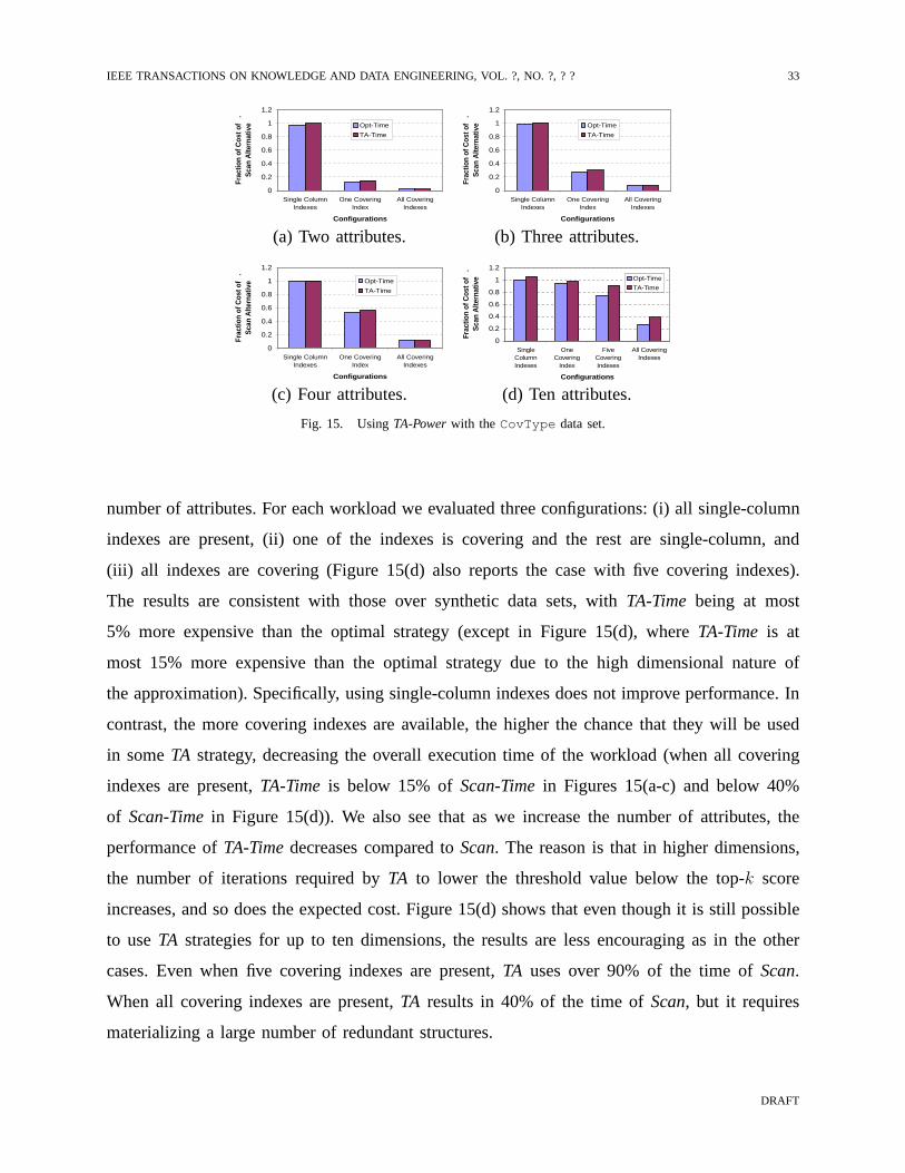
IEEE TRANSACTIONS ON KNOWLEDGE AND DATA ENGINEERING, VOL. ?, NO. ?, ? ? 33
0
0.2
0.4
0.6
0.8
1
1.2
Single ColumnIndexes
One CoveringIndex
All CoveringIndexes
Configurations
Frac
tion
of C
ost o
f .
Sca
n A
ltern
ativ
e Opt-Time
TA-Time
0
0.2
0.4
0.6
0.8
1
1.2
Single ColumnIndexes
One CoveringIndex
All CoveringIndexes
Configurations
Frac
tion
of C
ost o
f .
Sca
n A
ltern
ativ
e Opt-Time
TA-Time
(a) Two attributes. (b) Three attributes.
0
0.2
0.4
0.6
0.8
1
1.2
Single ColumnIndexes
One CoveringIndex
All CoveringIndexes
Configurations
Frac
tion
of C
ost o
f .
Sca
n A
ltern
ativ
e Opt-Time
TA-Time
0
0.2
0.4
0.6
0.8
1
1.2
SingleColumnIndexes
OneCovering
Index
FiveCoveringIndexes
All CoveringIndexes
Configurations
Frac
tion
of C
ost o
f .
Sca
n A
ltern
ativ
e Opt-Time
TA-Time
(c) Four attributes. (d) Ten attributes.
Fig. 15. UsingTA-Powerwith theCovType data set.
number of attributes. For each workload we evaluated three configurations: (i) all single-column
indexes are present, (ii) one of the indexes is covering and the rest are single-column, and
(iii) all indexes are covering (Figure 15(d) also reports the case with five covering indexes).
The results are consistent with those over synthetic data sets, with TA-Time being at most
5% more expensive than the optimal strategy (except in Figure 15(d), whereTA-Time is at
most 15% more expensive than the optimal strategy due to the high dimensional nature of
the approximation). Specifically, using single-column indexes does not improve performance. In
contrast, the more covering indexes are available, the higher the chance that they will be used
in someTA strategy, decreasing the overall execution time of the workload (when all covering
indexes are present,TA-Time is below 15% ofScan-Timein Figures 15(a-c) and below 40%
of Scan-Timein Figure 15(d)). We also see that as we increase the number ofattributes, the
performance ofTA-Timedecreases compared toScan. The reason is that in higher dimensions,
the number of iterations required byTA to lower the threshold value below the top-k score
increases, and so does the expected cost. Figure 15(d) showsthat even though it is still possible
to useTA strategies for up to ten dimensions, the results are less encouraging as in the other
cases. Even when five covering indexes are present,TA uses over 90% of the time ofScan.
When all covering indexes are present,TA results in 40% of the time ofScan, but it requires
materializing a large number of redundant structures.
DRAFT
IEEE TRANSACTIONS ON KNOWLEDGE AND DATA ENGINEERING, VOL. ?, NO. ?, ? ? 34
D. Impact of Greedy Search
We re-evaluated all workloads using bothTA-Powerand TA-Power-Greedy. In all but three
cases, the resulting execution plans were exactly the same for both techniques. For the remaining
three cases,TA-Power-Greedyresulted in less than 2% degradation with respect toTA-Power,
by examining a fraction of the space ofTA strategies.
VI. CONCLUSIONS
In this work we studied whether recent algorithms proposed to efficiently answer top-k queries
in middleware systems could be adapted to work in the contextof a RDBMS. We identified
the main challenges in adapting theTA algorithm to work inside the relational engine. As with
traditional relational processing, the choice of indexes critically determines the execution cost
of TA strategies. We identified the space of execution alternatives, designed a cost model based
on power laws to approximate the cost of each alternative, and provided pruning rules to speed
up query optimization. We then showed experimentally that in general,TA strategies based on
single-column indexes are rarely more efficient than simplesequential scans over the underlying
table unless the data is extremely correlated. However, if one or more covering indexes are
available, the improvement given by the bestTA strategy can be of orders of magnitude. We do
not expect covering indexes to be built just for answering a given top-k query (in fact, if that were
the case, we would be using a full sequential scan to build theindex as a prerequisite for aTA
strategy, which defeats its purpose). In contrast, we believe that for given query workloads, the
cost of building a useful set of indexes (once) would be amortized by a large number of queries
that subsequently benefit from such indexes. As usual, one needs to be careful since each new
index adds overhead for update statements in the workload, but this is the same trade-off that
occurs in traditional query processing. We see physical design tuning as an orthogonal problem.
Deciding which indexes to create for a given top-k query workload is a very important problem
but it lies outside of the scope of this work. Although some ofour results seem intuitive, this
is the first quantitative evaluation of relying onTA-like techniques to answer top-k queries in a
RDBMS. Our conclusion is that it is good to incorporate our adaptedTA strategies to the set of
algorithms that a relational optimizer can take advantage of to efficiently evaluate queries.
DRAFT
IEEE TRANSACTIONS ON KNOWLEDGE AND DATA ENGINEERING, VOL. ?, NO. ?, ? ? 35
REFERENCES
[1] G. Salton,Automatic Text Processing: The transformation, analysis,and retrieval of information by computer. Addison-
Wesley, 1989.
[2] D. Aksoy and M. Franklin, “RxW: a scheduling approach forlarge-scale on-demand data broadcast,”ACM Transsactions
on Networking, vol. 7, no. 6, pp. 846–860, 1999.
[3] A. Marian, N. Bruno, , and L. Gravano, “Evaluating top-k queries over web-accessible databases,”ACM Transactions on
Database Systems (TODS), vol. 29, no. 2, pp. 319–362, 2004.
[4] R. Fagin, A. Lotem, and M. Naor, “Optimal aggregation algorithms for middleware,” inProc. of the Twentieth ACM
Symposium on Principles of Database Systems, 2001, pp. 102 – 113.
[5] I. Ilyas et al., “Rank-aware query optimization,” inProceedings of the ACM International Conference on Management of
Data (SIGMOD), 2004, pp. 203–214.
[6] M. J. Carey and D. Kossmann, “On saying “Enough Already!”in SQL,” in Proceedings of the 1997 ACM International
Conference on Management of Data, 1997, pp. 219–230.
[7] N. Bruno, S. Chaudhuri, and L. Gravano, “Top-k selection queries over relational databases: Mapping strategies and
performance evaluation,”ACM Transactions on Database Systems (TODS), vol. 27, no. 2, pp. 153–187, 2002.
[8] C.-M. Chen and Y. Ling, “A sampling-based estimator for Top-k query,” inProceedings of the International Conference
on Data Engineering (ICDE), 2002, pp. 617–627.
[9] U. Guntzer, W.-T. Balke, and W. Kießling, “Optimizing multi-feature queries for image databases,” inProceedings of the
International Conference on Very Large Databases, 2000, pp. 419–428.
[10] S. Nepal and M. V. Ramakrishna, “Query processing issues in image (multimedia) databases,” inProceedings of the
International Conference on Data Engineering, 1999, pp. 22–29.
[11] K. Chang and S. won Hwang, “Minimal probing: supportingexpensive predicates for top-k queries,” inProceedings of
the ACM International Conference on Management of Data (SIGMOD), 2002, pp. 346–357.
[12] E. Wimmers, L. Haas, M. T. Roth, and C. Braendli, “Using Fagin’s algorithm for merging ranked results in multimedia
middleware,” inInternational Conference on Cooperative Information Systems (CoopIS), 1999, pp. 267–278.
[13] R. Fagin, “Combining fuzzy information from multiple systems,” inProceedings of the Fifteenth ACM Symposium on
Principles of Database Systems (PODS’96), 1996, pp. 216–226.
[14] C. Lang, Y.-C. Chang, and J. Smith, “Making the threshold algorithm access cost aware,”IEEE Transactions on Knowledge
and Data Engineering, vol. 16, no. 10, pp. 1297– 1301, 2004.
[15] N. Bruno, S. Chaudhuri, and L. Gravano, “STHoles: A multidimensional workload-aware histogram,” inProceedings of
the ACM International Conference on Management of Data (SIGMOD), 2001, pp. 211–222.
[16] D. Gunopuloset al., “Approximating multi-dimensional aggregate range queries over real attributes,” inProceedings of
the ACM International Conference on Management of Data (SIGMOD), 2000, pp. 463–474.
[17] C. Blake and C. Merz, “UCI repository of machine learning databases,” 1998,
ftp://ftp.ics.uci.edu/pub/machine-learning-database/covtype.
DRAFT


![RSA Threshold Cryptography · 3.3 RSA Algorithm ... and decryption algorithm [16]. ... they are also used as the bench mark to test new ideas in](https://img.dokumen.tips/doc/110x75/5ae413827f8b9a495c8e0d3b/rsa-threshold-cryptography-rsa-algorithm-and-decryption-algorithm-16-.jpg)