The Term Structure of Variance Swaps, Risk Premia and the ...The Term Structure of Variance Swaps, Risk Premia and the Expectation Hypothesis ... which in the case of the S&P500 is

The Term Structure of Variance Swaps, RiskPremia and the Expectation Hypothesis

Yacine A��t-Sahalia Mustafa Karaman Loriano ManciniPrinceton University University of Z�urich EPFL

1

1 INTRODUCTION

1. Introduction

� Among volatility derivatives, Variance Swaps are simple contracts:

{ the �xed leg agrees at inception that it will pay a �xed amount at

maturity T , the VS rate

{ in exchange to receiving a oating amount based on the realized

variance of the underlying asset from 0 to T:

� One potential di�culty lies in the path-dependency introduced by therealized variance.

2

1 INTRODUCTION

� But the payo� of a VS can be replicated by dynamic trading in theunderlying asset and a static position in vanilla options

{ This insight, originally due to Neuberger (1994) and Dupire (1993),means that the path-dependency implicit in VS could be circum-vented

{ It also made possible the analysis of the various hedging errorswhen attempting to replicate a given VS (see, e.g., Carr andMadan (1998), Britten-Jones and Neuberger (2000), Jiang andTian (2005), Jiang and Oomen (2008), Carr and Wu (2009), Carrand Lee (2010).)

{ Because of the interest in replicating a given contract, VS rateshave generally been studied at a single maturity.

{ Including a determination of the variance risk premia at a singleshort maturity: see Carr and Wu (2009), Todorov (2010), Bollerslevand Todorov (2011a) and Bollerslev and Todorov (2011b).

3

1 INTRODUCTION

� But VS rates give rise naturally to a term structure, by varying the

maturity at which the exchange of cash ows take place

{ The literature has proceded by analogy with the term structure of

interest rates

{ Including determining the number of factors necessary to capture

the variation of the curve (see B�uhler (2006), Gatheral (2008),

Amengual (2008) and Eglo� et al. (2010).)

4

1 INTRODUCTION

� We continue this line of research with two di�erences:

{ First, we do not proceed fully by analogy with the term structure

of interest rates, i.e., by taking either the variances themselves or

their latent factors as the primitives

� Instead, we incorporate the fact that the variance in a VS is thatof an underlying asset

� This means that we can infer properties of the risk premia asso-ciated not just with the variances but also with the asset itself,

which in the case of the S&P500 is the classical equity risk pre-

mium.

{ Second, we allow for the presence of jumps in asset returns.

5

1 INTRODUCTION

� Various aspects of the VS term structure cannot be studied in a model-free manner, because the necessary data are either insu�cient in quan-

tity or simply unavailable.

{ We work with a parametric stochastic volatility model which is con-

sistent with the salient empirical features of VS rates documented

in the model-free analysis.

{ The model is estimated using maximum-likelihood, combining time

series information on stock returns and cross sectional information

on the term structure of VS rates.

6

1 INTRODUCTION

� The model allows the risk premia to be estimated in a term structure

framework

{ the variance risk premium

{ and the equity risk premium

� We study whether the Expectation Hypothesis (EH) holds in the termstructure of VS.

� Finally, to assess the economic pro�tability of VS contracts, we developa simple but robust trading strategy involving VS: as the ex-ante vari-

ance risk premium is found to be negative, the strategy takes a short

position in the VS contract .

7

2 VARIANCE SWAP RATES

2. Variance Swap Rates

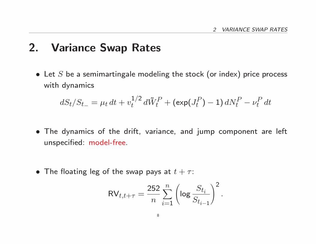
� Let S be a semimartingale modeling the stock (or index) price processwith dynamics

dSt=St� = �t dt+ v1=2t d ~WP

t + (exp(JPt )� 1) dNPt � �Pt dt

� The dynamics of the drift, variance, and jump component are leftunspeci�ed: model-free.

� The oating leg of the swap pays at t+ � :

RVt;t+� =252

n

nXi=1

log

StiSti�1

!2:

8


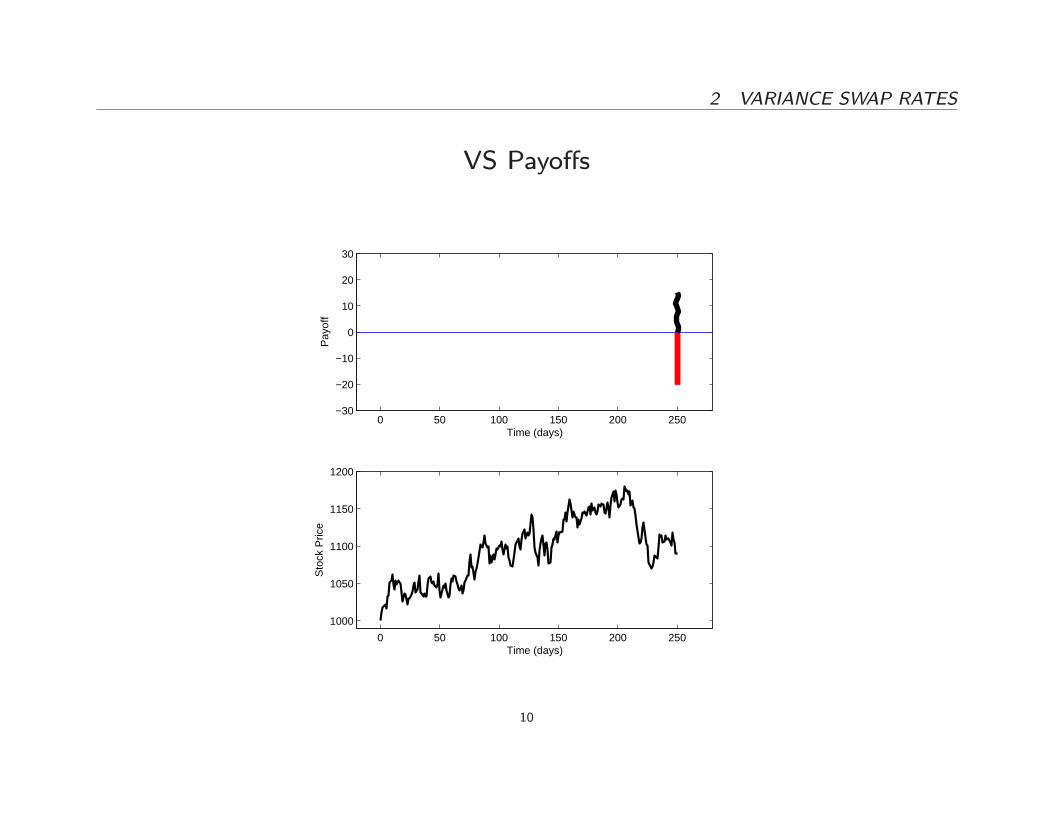
� Like any swap, no cash ow changes hands at inception of the contractat time t; the �xed leg of the variance swap agrees to pay an amount

�xed at time t, de�ned as the variance swap rate, VSt;t+� :

{ Therefore, at maturity, t+ � , the long position in a variance swap

contract receives the di�erence between the realized variance be-

tween times t and t + � , RVt;t+� , and the variance swap rate,

VSt;t+� , which was �xed at time t.

{ The di�erence is multiplied by a �xed notional amount to convert

the payo� to dollar terms:

(RVt;t+� � VSt;t+�)� notional:

9


VS Payo�s

0 50 100 150 200 250−30

−20

−10

0

10

20

30

Time (days)

Pay

off

0 50 100 150 200 250

1000

1050

1100

1150

1200

Time (days)

Sto

ck P

rice

10


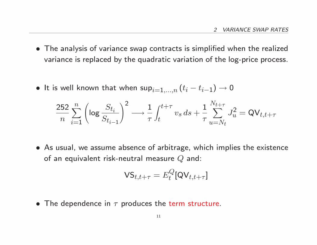
� The analysis of variance swap contracts is simpli�ed when the realizedvariance is replaced by the quadratic variation of the log-price process.

� It is well known that when supi=1;:::;n (ti � ti�1)! 0

252

n

nXi=1

log

StiSti�1

!2�! 1

�

Z t+�t

vs ds+1

�

Nt+�Xu=Nt

J2u = QVt;t+�

� As usual, we assume absence of arbitrage, which implies the existenceof an equivalent risk-neutral measure Q and:

VSt;t+� = EQt [QVt;t+� ]

� The dependence in � produces the term structure.

11

2.1 Preliminary Data Analysis 2 VARIANCE SWAP RATES

2.1. Preliminary Data Analysis

� Dataset: OTC quotes on VS on the S&P500 provided by a major

broker-dealer in New York City.

� The data are daily closing quotes on variance swap rates with �xedtime to maturities of 2, 3, 6, 12, and 24 months from January 4,

1996 to September 2, 2010, resulting in 3,624 observations for each

maturity.

12


The Term Structure of VS Rates

97 98 99 00 01 02 03 04 05 06 07 08 09 10 236

12

24

10

20

30

40

50

60

70

80

Maturity months

Year

Var

ianc

e S

wap

Rat

e %

13


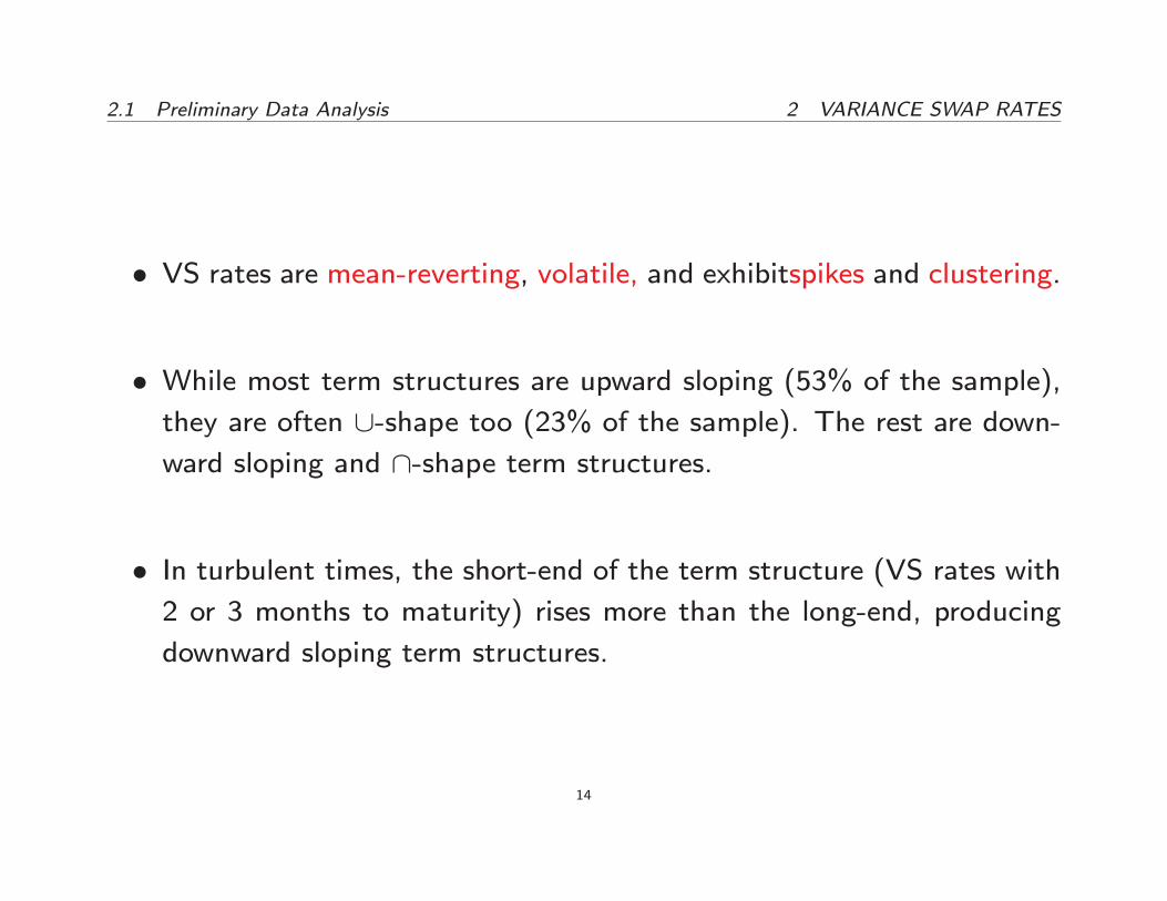
� VS rates are mean-reverting, volatile, and exhibitspikes and clustering.

� While most term structures are upward sloping (53% of the sample),

they are often [-shape too (23% of the sample). The rest are down-

ward sloping and \-shape term structures.

� In turbulent times, the short-end of the term structure (VS rates with

2 or 3 months to maturity) rises more than the long-end, producing

downward sloping term structures.

14


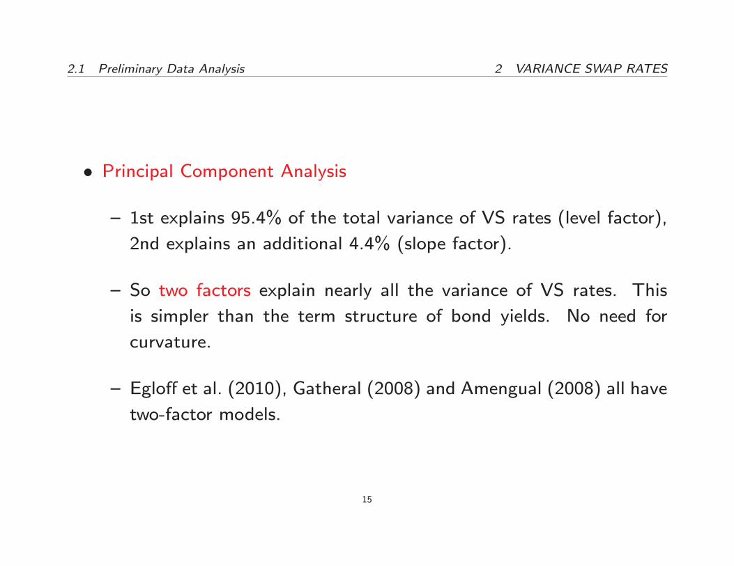
� Principal Component Analysis

{ 1st explains 95.4% of the total variance of VS rates (level factor),

2nd explains an additional 4.4% (slope factor).

{ So two factors explain nearly all the variance of VS rates. This

is simpler than the term structure of bond yields. No need for

curvature.

{ Eglo� et al. (2010), Gatheral (2008) and Amengual (2008) all have

two-factor models.

15


Principal Component Analysis of VS Rates

0 5 10 15 20 25−0.6

−0.4

−0.2

0

0.2

0.4

0.6

0.8

Time to maturity in months

Factor 1Factor 2

16

2.2 Model-Free Jump Component in VS 2 VARIANCE SWAP RATES

2.2. Model-Free Jump Component in VS

� We start with the model-free method (see Neuberger (1994), Dupire(1993), Carr and Madan (1998), Demeter� et al. (1999), Britten-

Jones and Neuberger (2000), Jiang and Tian (2005), Jiang and Oomen

(2008), Carr and Wu (2009) and Carr and Lee (2010).)

� The replication is model-free in the sense that the stock price canfollow the general model, but with the restriction �t = 0 and/or Jt =

0.

17


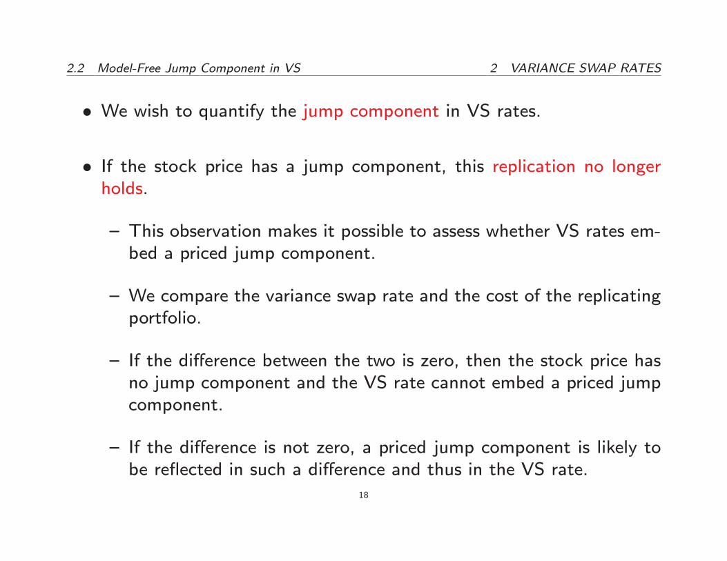
� We wish to quantify the jump component in VS rates.

� If the stock price has a jump component, this replication no longerholds.

{ This observation makes it possible to assess whether VS rates em-bed a priced jump component.

{ We compare the variance swap rate and the cost of the replicatingportfolio.

{ If the di�erence between the two is zero, then the stock price hasno jump component and the VS rate cannot embed a priced jumpcomponent.

{ If the di�erence is not zero, a priced jump component is likely tobe re ected in such a di�erence and thus in the VS rate.

18


VSt;t+� = EQt [QVt;t+� ]

=2

�

Z 10

�t(K; t+ �)

K2dK

+2

�EQt

Nt+�Xu=Nt

"J2u2+ Ju + 1� exp(Ju)

#

= VIXt;t+� +2

�EQt

Nt+�Xu=Nt

"J2u2+ Ju + 1� exp(Ju)

#

� �t(K; t + �) is the time-t forward price of the out-of-the-money putor call option with strike K and maturity t+ � .

� VIXt;t+� is then the variance swap rate, VSt;t+� , when the stock pricehas no jump component.

19


� The key point for what follows is that the di�erence VSt;t+��VIXt;t+�is (up to the discretization error) a model-free measure of the jump

component in VS rates, i.e., the last term above.

{ If the jump component is zero, i.e., the jump size Ju = 0 and/or the

intensity of the counting processNt is zero, then VSt;t+��VIXt;t+�is zero as well.

{ If the jump component is not zero and priced, then VSt;t+� �VIXt;t+� tends to be positive.

{ The reason is that the jump term in the square brackets is down-

ward sloping and passing through the origin.

{ If the jump distribution under Q is shifted to the left, suggesting

that jump risk is priced, the last expectation tends to be positive.

20


Time Series of VSt;t+� � VIXt;t+� for Di�erent Maturities

97 98 99 00 01 02 03 04 05 06 07 08 09 10−10

−5

0

5

10

15

20

25

Year

VS

min

us V

IX %

In−Sample Out−of−Sample

2−month3−month6−month

21


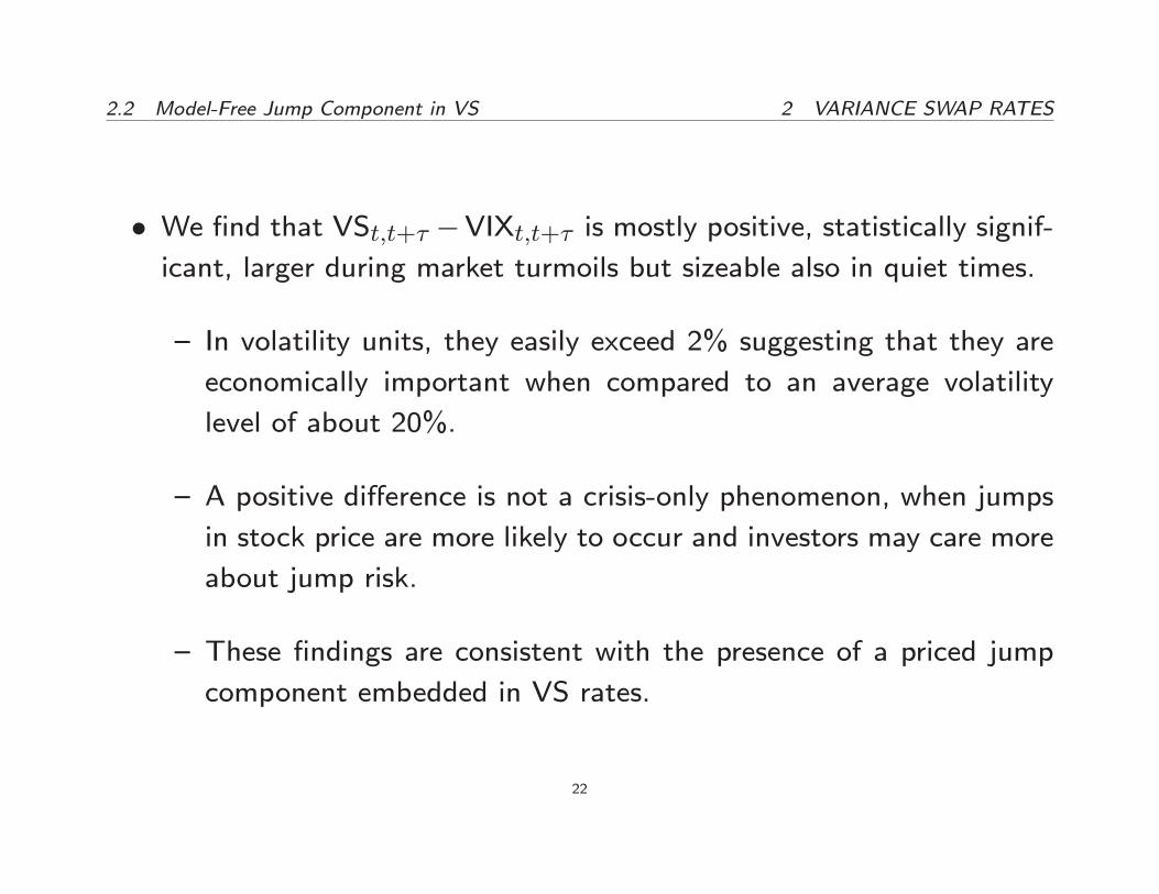
� We �nd that VSt;t+� �VIXt;t+� is mostly positive, statistically signif-icant, larger during market turmoils but sizeable also in quiet times.

{ In volatility units, they easily exceed 2% suggesting that they are

economically important when compared to an average volatility

level of about 20%.

{ A positive di�erence is not a crisis-only phenomenon, when jumps

in stock price are more likely to occur and investors may care more

about jump risk.

{ These �ndings are consistent with the presence of a priced jump

component embedded in VS rates.

22

2.3 A Parametric Stochastic Volatility Model 2 VARIANCE SWAP RATES

2.3. A Parametric Stochastic Volatility Model

� The limitations of the data available make it necessary to adopt aparametric structure, with a speci�cation informed by the model-free

analysis above, in order to go further.

dSt=St� = �tdt+ (1� �2)1=2v

1=2t dWP

1t

+ �v1=2t dWP

2t + (exp(JPt )� 1) dNt � �Pt dt

dvt = kPv (mt k

Qv =k

Pv � vt)dt+ �vv

1=2t dWP

2t

dmt = kPm(�

Pm �mt)dt+ �mm

1=2t dWP

3t

where �t = r � � + 1(1 � �2)vt + 2�vt + (gP � gQ)�t, r is the

risk free rate and � the dividend yield, both taken to be constant for

simplicity only.

23


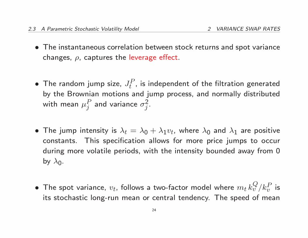
� The instantaneous correlation between stock returns and spot variancechanges, �, captures the leverage e�ect.

� The random jump size, JPt , is independent of the �ltration generated

by the Brownian motions and jump process, and normally distributed

with mean �Pj and variance �2j .

� The jump intensity is �t = �0 + �1vt, where �0 and �1 are positive

constants. This speci�cation allows for more price jumps to occur

during more volatile periods, with the intensity bounded away from 0

by �0.

� The spot variance, vt, follows a two-factor model where mt kQv =kPv isits stochastic long-run mean or central tendency. The speed of mean

24


reversion is kPv under P , kQv under Q and kPv = k

Qv � 2�v, where 2

is the market price of risk for WP2t ;

� The stochastic long run mean of vt is controlled bymt which follows itsown stochastic mean reverting process and mean reverts to a positive

constant �Pm, when the speed of mean reversion kPm is positive.

� Typically, vt is fast mean reverting and volatile to capture suddenmovements in volatility, while mt is more persistent and less volatile

to capture long term movements in volatility.

25


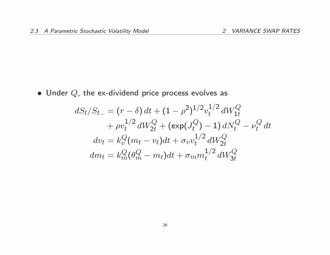
� Under Q, the ex-dividend price process evolves as

dSt=St� = (r � �) dt+ (1� �2)1=2v

1=2t dW

Q1t

+ �v1=2t dW

Q2t + (exp(J

Qt )� 1) dN

Qt � �

Qt dt

dvt = kQv (mt � vt)dt+ �vv

1=2t dW

Q2t

dmt = kQm(�

Qm �mt)dt+ �mm

1=2t dW

Q3t

26

2.4 The Term Structure of VS Rates 2 VARIANCE SWAP RATES

2.4. The Term Structure of VS Rates

� Given the stochastic volatility model above, VS rates can be calculated:

VSt;t+� =1

�

Z t+�t

EQt [vs]ds+

1

�EQ[J2]E

Qt [Nt+� �Nt]

= EQ[J2]�0 + (1 + �1EQ[J2])

� [(1� �Qv (�)� �Qm(�))�Qm + �Qv (�)vt + �Qm(�)mt]

where EQ[J2] = EQt [J

2], as the random jump size is time-homogeneous,

and

�Qv (�) =(1� e�k

Qv �)

kQv �

�Qm(�) =

�1 + e�k

Qv �k

Qm=(k

Qv � kQm)� e�k

Qm�k

Qv =(k

Qv � kQm)

�kQm�

27

2.4 The Term Structure of VS Rates 2 VARIANCE SWAP RATES

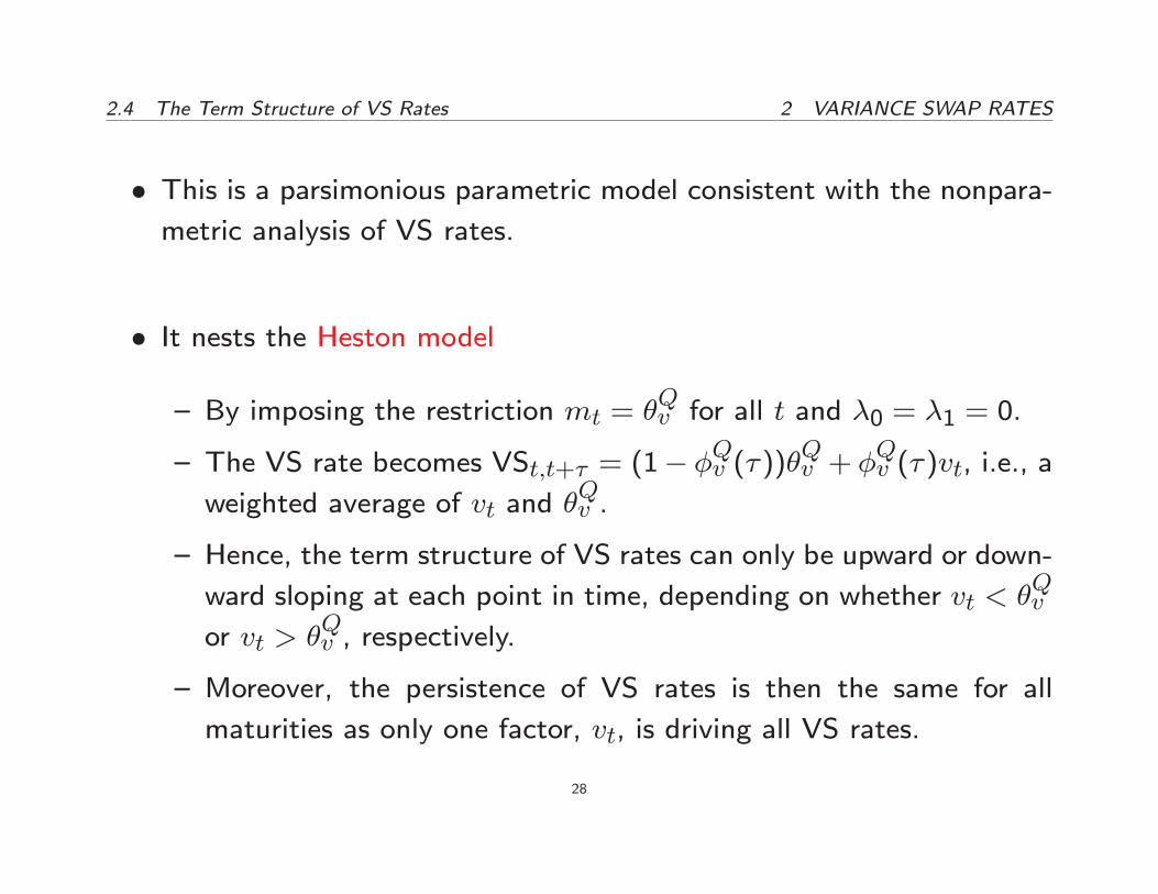
� This is a parsimonious parametric model consistent with the nonpara-metric analysis of VS rates.

� It nests the Heston model

{ By imposing the restriction mt = �Qv for all t and �0 = �1 = 0.

{ The VS rate becomes VSt;t+� = (1� �Qv (�))�Qv + �Qv (�)vt, i.e., aweighted average of vt and �

Qv .

{ Hence, the term structure of VS rates can only be upward or down-

ward sloping at each point in time, depending on whether vt < �Qv

or vt > �Qv , respectively.

{ Moreover, the persistence of VS rates is then the same for all

maturities as only one factor, vt, is driving all VS rates.

28

3 LIKELIHOOD-BASED ESTIMATION

3. Likelihood-Based Estimation

� The procedure we employ then combines time series information on theS&P500 returns and cross sectional information on the term structures

of VS rates in the same spirit as in other derivative pricing contexts

� Hence, P and Q parameters, including risk premia, are estimated

jointly by exploiting the internal consistency of the model, thereby

making the inference procedure theoretically sound.

� Let X 0t = [log(St); Y 0t ] denote the state vector, where Yt = [vt;mt]0 islatent and will be extracted from actual VS rates.

29


� Likelihood-based estimation requires evaluation of the likelihood func-tion of index returns and term structures of variance swap rates for

each parameter vector during a likelihood search.

� The procedure for evaluating the likelihood function consists of thefollowing steps.

{ First, we extract the unobserved state vector Yt from a set of

benchmark variance swap rates, assumed to be observed without

error: 264 VSt;t+�1...VSt;t+�`

375 =264 a(�1; �)...a(�`; �)

375+264 b(�1; �)0...b(�`; �)

0

375Yt30


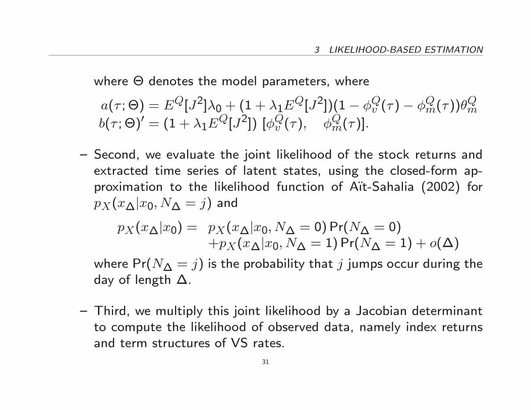
where � denotes the model parameters, where

a(� ; �) = EQ[J2]�0 + (1 + �1EQ[J2])(1� �Qv (�)� �Qm(�))�Qm

b(� ; �)0 = (1 + �1EQ[J2]) [�Qv (�); �Qm(�)]:

{ Second, we evaluate the joint likelihood of the stock returns andextracted time series of latent states, using the closed-form ap-proximation to the likelihood function of A��t-Sahalia (2002) forpX(x�jx0; N� = j) and

pX(x�jx0) = pX(x�jx0; N� = 0)Pr(N� = 0)+pX(x�jx0; N� = 1)Pr(N� = 1) + o(�)

where Pr(N� = j) is the probability that j jumps occur during theday of length �.

{ Third, we multiply this joint likelihood by a Jacobian determinantto compute the likelihood of observed data, namely index returnsand term structures of VS rates.

31


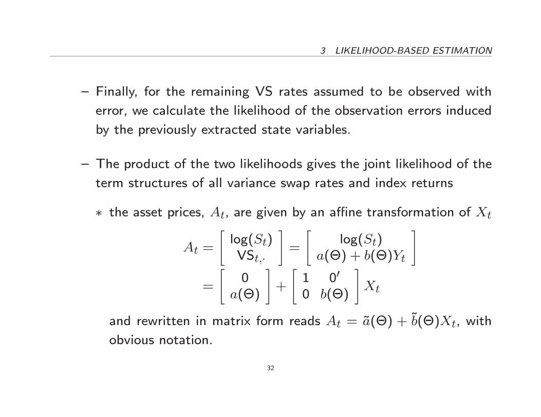
{ Finally, for the remaining VS rates assumed to be observed with

error, we calculate the likelihood of the observation errors induced

by the previously extracted state variables.

{ The product of the two likelihoods gives the joint likelihood of the

term structures of all variance swap rates and index returns

� the asset prices, At, are given by an a�ne transformation of Xt

At =

"log(St)VSt;�

#=

"log(St)

a(�) + b(�)Yt

#

=

"0

a(�)

#+

"1 00

0 b(�)

#Xt

and rewritten in matrix form reads At = ~a(�) + ~b(�)Xt, with

obvious notation.

32


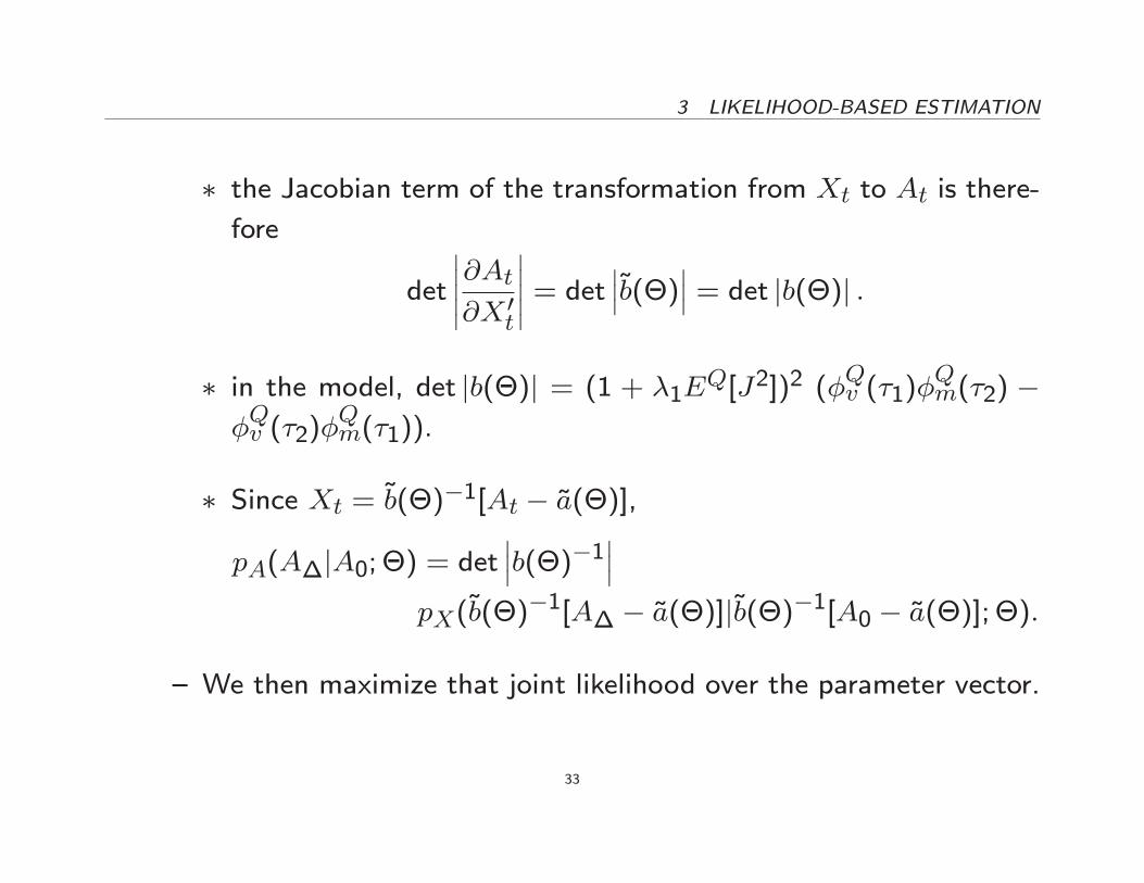
� the Jacobian term of the transformation from Xt to At is there-

fore

det

��@At@X 0t

�� = det ��~b(�)�� = det jb(�)j :� in the model, det jb(�)j = (1 + �1E

Q[J2])2 (�Qv (�1)�

Qm(�2) �

�Qv (�2)�

Qm(�1)).

� Since Xt = ~b(�)�1[At � ~a(�)],

pA(A�jA0; �) = det��b(�)�1��

pX(~b(�)�1[A� � ~a(�)]j~b(�)�1[A0 � ~a(�)]; �):

{ We then maximize that joint likelihood over the parameter vector.

33

4 FITTING VARIANCE SWAP RATES

4. Fitting Variance Swap Rates

4.1. In-Sample Estimation

� We use as in-sample for estimation the period from January 4, 1996

to April 2, 2007.

34

4.1 In-Sample Estimation 4 FITTING VARIANCE SWAP RATES

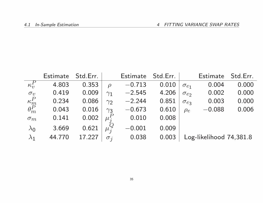
Estimate Std.Err. Estimate Std.Err. Estimate Std.Err.

�Pv 4.803 0.353 � �0.713 0.010 �e1 0.004 0.000�v 0.419 0.009 1 �2.545 4.206 �e2 0.002 0.000

�Pm 0.234 0.086 2 �2.244 0.851 �e3 0.003 0.000

�Pm 0.043 0.016 3 �0.673 0.610 �e �0.088 0.006

�m 0.141 0.002 �Pj 0.010 0.008

�0 3.669 0.621 �Qj �0.001 0.009

�1 44.770 17.227 �j 0.038 0.003 Log-likelihood 74,381.8

35


� The spot variance is relatively fast mean-reverting as kPv implies a

half-life of 36 days.

� Its stochastic long run mean is slowly mean reverting with a half-lifeof almost 3 years.

� The instantaneous volatility of vt is almost 3 times that of mt.

� The correlation between stock returns and variance changes, �, is�0:7,con�rming the presence of a strong leverage e�ect.

� The long-run average volatility is 21%36


� Both 2 and 3 are negative, implying negative instantaneous variancerisk premia.

� The correlation parameter for the VS pricing errors, �e, is close to 0,suggesting that the model does not produce systematic pricing errors.

� The expected jump size is positive under the objective probability mea-sure, �Pj , and slightly negative under the risk-neutral measure, �

Qj ,

suggesting a positive jump risk premium.

� Estimates of jump intensity implies six jumps per year on average.

37


� We also estimate three nested models:

{ two-factor model with constant jump intensity (setting �1 = 0)

{ two-factor model with no jump component (setting �0 = �1 = 0)

{ the Heston model (setting �0 = �1 = 0 and mt = �Pv for all t).

� The nested models are rejected: each restriction signi�cantly deterio-rates the joint �t of VS rates and S&P500 returns.

38

4.2 Out-of-Sample 4 FITTING VARIANCE SWAP RATES

4.2. Out-of-Sample

� We conduct all subsequent analyses using two subsamples.

� Data from January 4, 1996 to April 2, 2007 are used for in-sampleestimation.

� The remaining sample data, from April 3, 2007 to September 2, 2010,are used for out-of-sample analysis and robustness checks.

� The second subsample includes the �nancial crisis of Fall 2008 whichwas not experienced (nor likely anticipated) in the prior �tting sample.

� We compute pricing errors, the model-based VS rate minus the ob-served VS rate

39


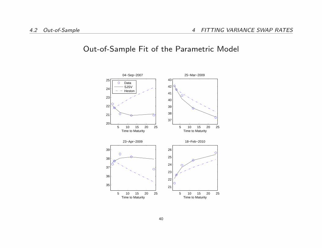
Out-of-Sample Fit of the Parametric Model

5 10 15 20 2520

21

22

23

24

25

Time to Maturity

04−Sep−2007

DataSJSVHeston

5 10 15 20 25

37

38

39

40

41

42

43

Time to Maturity

25−Mar−2009

5 10 15 20 25

35

36

37

38

39

Time to Maturity

23−Apr−2009

5 10 15 20 25

21

22

23

24

25

26

Time to Maturity

18−Feb−2010

40


� The model �ts VS rates well both in- and out-of-sample and signi�-cantly outperforms the Heston model.

� For example, its RMSE is 6 times smaller than that of the Hestonmodel when �tting 24-month to maturity VS rates.

41

5 RISK PREMIA: EQUITY AND VOLATILITY

5. Risk Premia: Equity and Volatility

� One advantage of modeling the underlying asset returns jointly withthe VS rates is that the resulting model produces estimates of risk

premia for both sets of variables, including in particular estimates of

the classical equity premium.

� We distinguish between the spot or instantaneous risk premia at eachinstant t and the integrated ones, de�ned over each maturity � .

� In each case, the model provides a natural breakdown between thecontinuous and jump components of the respective risk premia.

42

5 RISK PREMIA: EQUITY AND VOLATILITY

� Results

{ We �nd an important role of the jump component in the spot

equity risk premium.

{ The longer the maturity, the larger the negative risk premium,

especially during turbulent times.

{ Market crashes impact and propagate di�erently throughout the

term structure, with the short-end being more a�ected, but the

long-end exhibiting more persistency.

43

5.1 Spot Risk Premia 5 RISK PREMIA: EQUITY AND VOLATILITY

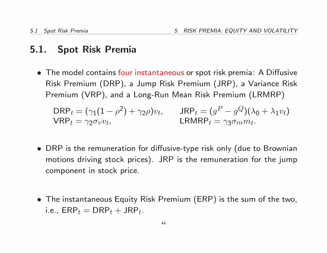
5.1. Spot Risk Premia

� The model contains four instantaneous or spot risk premia: A Di�usiveRisk Premium (DRP), a Jump Risk Premium (JRP), a Variance Risk

Premium (VRP), and a Long-Run Mean Risk Premium (LRMRP)

DRPt = ( 1(1� �2) + 2�)vt, JRPt = (gP � gQ)(�0 + �1vt)

VRPt = 2�vvt, LRMRPt = 3�mmt.

� DRP is the remuneration for di�usive-type risk only (due to Brownianmotions driving stock prices). JRP is the remuneration for the jump

component in stock price.

� The instantaneous Equity Risk Premium (ERP) is the sum of the two,

i.e., ERPt = DRPt + JRPt.

44


� The mean growth rates of vt and mt are di�erent under the proba-bility measures P and Q, and such di�erences are given by VRPt and

LRMRPt, respectively.

� As 2 and 3 are estimated to be negative, VRP and LRMRP are bothnegative, and on average vt and mt are higher under Q than under P .

45


� The negative sign of the variance risk premium is not abnormal.

{ The risk premium for return risk is positive, because investors re-

quire a higher rate of return as compensation for return risk.

{ On the other hand, investors require a lower level of variance as

compensation for variance risk, hence the negative variance risk

premium.

{ Risk-averse investors dislike both higher return variance and higher

variance of the return variance.

46


� During our in-sample period, January 1996 to April 2007, the averageERP is 6.8%.

{ Notably, 5.5% is due to the jump risk premium, which thus ac-

counts for a large fraction of the equity risk premium.

{ Jumps in prices are rare events, but jump risk is important as it

cannot be hedged easily.

{ The average VRP is also substantial and around �3:4%, while theLRMRP is much lower and around �0:4%.

{ During the out-of-sample period, April 2007 to September 2010,

all risk premia nearly doubled re ecting the unprecedented turmoil

in �nancial markets.

47

5.2 Integrated Risk Premia 5 RISK PREMIA: EQUITY AND VOLATILITY

5.2. Integrated Risk Premia

� The annualized integrated Equity Risk Premium (IERP) is de�ned as

IERPt;t+� = EPt [St+�=St]=� � E

Qt [St+�=St]=�

and represents the expected excess return from buying and holding the

S&P500 index from t to t+ � .

� Extensive research has been devoted to study levels and dynamicsof the IERP, in particular investigating the so-called equity premium

puzzle.

� Much less attention has been devoted to study the term structure of

the IERP.48


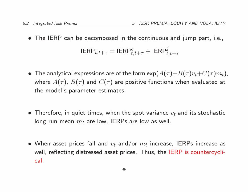
� The IERP can be decomposed in the continuous and jump part, i.e.,

IERPt;t+� = IERPct;t+� + IERP

jt;t+�

� The analytical expressions are of the form exp(A(�)+B(�)vt+C(�)mt),where A(�), B(�) and C(�) are positive functions when evaluated at

the model's parameter estimates.

� Therefore, in quiet times, when the spot variance vt and its stochasticlong run mean mt are low, IERPs are low as well.

� When asset prices fall and vt and/or mt increase, IERPs increase aswell, re ecting distressed asset prices. Thus, the IERP is countercycli-

cal.49


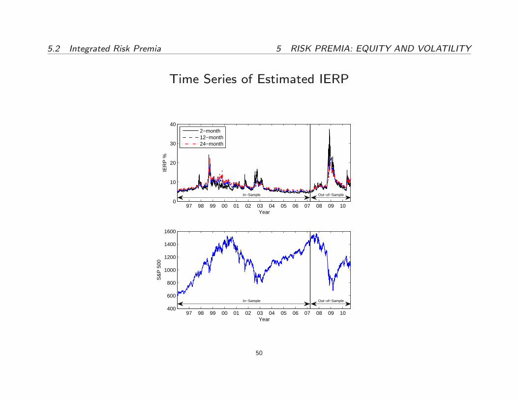
Time Series of Estimated IERP

97 98 99 00 01 02 03 04 05 06 07 08 09 100

10

20

30

40

Year

IER

P %


2−month12−month24−month

97 98 99 00 01 02 03 04 05 06 07 08 09 10400

600

800

1000

1200

1400

1600

Year

S&

P 5

00


50


� The entire term structure of the IERP exhibits signi�cant variation

over time, with the short-end being more volatile than the long-end.

� When the S&P500 steadily increased during 2005{07, the 2-monthIERP dropped at the lowest level, around 4.5%, during our sample

period.

� The term structure was upward sloping with the 24-month IERP at

6%.

� At the end of 2008 and beginning of 2009, the term structure of the

IERP became downward sloping with the 2-month IERP reaching its

highest value in decades.

51


� On November 20, 2008, the 2-month IERP was as high as 37%, andbetween October and December 2008, the IERP was above 25% on

various occasions, mirroring the fall of the index.

� Indeed, from mid-September to mid-November 2008, the S&P500 in-

dex dropped from 1,200 to 750, loosing 37% of its value.

� On March 9, 2009, it reached its lowest value in more than a decade, at677, and then recovered 35% of its value within the next two months.

Such large swings in the S&P500 index suggest that the large model-

based estimates of the IERP are reasonable.

52


� Integrated Variance Risk Premium

{ The annualized integrated variance risk premium (IVRP) is de�ned

as IVRPt;t+� = EPt [QVt;t+� ] � EQt [QVt;t+� ] and represents the

expected pro�t to the long side of a VS contract, which is entered

at time t and held till maturity t+ � .

{ Investors regard volatility increases as unfavorable events and are

willing to pay large premia, i.e., large VS rates, to insure against

such volatility increases.

{ The term structure of IVRP is on average downward sloping.

53


� We study the impact of negative jumps and the induced term structureof variance risk premia.

{ As many investors are \long in the market" and the leverage ef-fect is very pronounced, negative jump prices are perceived as un-

favorable events and thus can carry particular risk premia. The

contribution of negative jumps to the IVRP is given by

IVRP(k)jt;t+� = E

Pt [QV

jt;t+� 1fJ<kg]� E

Qt [QV

jt;t+� 1fJ<kg]

where 1fJ<kg is the indicator function of the event J < k.

{ We set k = �1%, i.e., we study the contribution of daily jumpsbelow �1% to the IVRP.

{ Between April 2007 and September 2010, the out-of-sample period,IVRP(k)

jt;t+� accounts for nearly half of the IVRP at the 2-month

horizon.54


Time Series of Estimated IVRP

97 98 99 00 01 02 03 04 05 06 07 08 09 10−6

−5

−4

−3

−2

−1

0


Year

IVR

P %

97 98 99 00 01 02 03 04 05 06 07 08 09 10−0.8

−0.7

−0.6

−0.5

−0.4

−0.3

−0.2

Year

IVR

P p

erce

ntag

e, J

< −

1%


2−month

12−month

24−month

55


� Similarly to the IVRP, the term structure of IVRP(k)jt;t+� is generally

downward sloping in quiet times.

� However, in contrast to IVRP, during market crashes the term structureof IVRP(k)

jt;t+� becomes suddenly upward sloping, re ecting the large

jump risk due to a price fall.

� In Fall 2008, the two-month IVRP(k)jt;t+� exhibited the largest nega-tive drop and took several months to revert to more normal values.

� This is consistent with investors' willingness to ensure against a marketcrash increasing after a price fall.

56

6 THE EXPECTATION HYPOTHESIS

6. The Expectation Hypothesis

� Several studies have investigated whether term structures of interest

rates, exchange rates or option implied volatilities can predict future

bond yields, spot exchange rates or underlying asset volatilities, re-

spectively.

� The traditional approach is to regress the variable of interest yt (e.g.,bond yield at time t) on a constant and its predictor xt (e.g., forward

rate at time t� 1 with maturity t).

� In the regression yt = �+� xt+"t, the hypothesis of interest is whetherthe predictor is unbiased, i.e., � = 0, and/or e�cient, i.e., � = 1, in

which case, the so-called Expectation Hypothesis (EH) holds.

� In our setting, a natural question is whether the VS rate provides anunbiased and/or e�cient prediction of future realized variance.

57


� The standard testing procedure would be to run a time series regressionof future, ex-post realized variance, QVt;t+� , on a constant and the

VS rate, VSt;t+� .

{ An alternative interpretation of the EH is in terms of risk premia.

By de�nition of IVRP, QVt;t+� = VSt;t+� + IVRPt;t+� + "t;t+� ,

where the last, zero mean, error term disappears when taking the

time-t conditional P -expectation.

{ This equation shows that if IVRPt;t+� is zero (or is stochastic

but with zero mean and uncorrelated with VSt;t+�), the regression

above would produce an intercept of zero and slope of one, i.e.,

EH would hold.

{ If IVRPt;t+� is constant (or is stochastic but with constant mean

and uncorrelated with VSt;t+�), the intercept would equal this con-

stant value and the slope would still be one.

58


{ If, indeed, IVRPt;t+� and VSt;t+� are driven by some common

factors (i.e., the two are correlated), when regressing the future

realized variance on the VS rate only, an important variable is

missing in the regression. IVRPt;t+� would be absorbed in the

regression error term, which would be correlated with the VS rate

regressor, producing inconsistent estimates.

{ Thus, the intercept will not be zero and the slope will not be one.

In other words, a rejection of the EH would imply a non-trivial

dynamic of the IVRP.

59


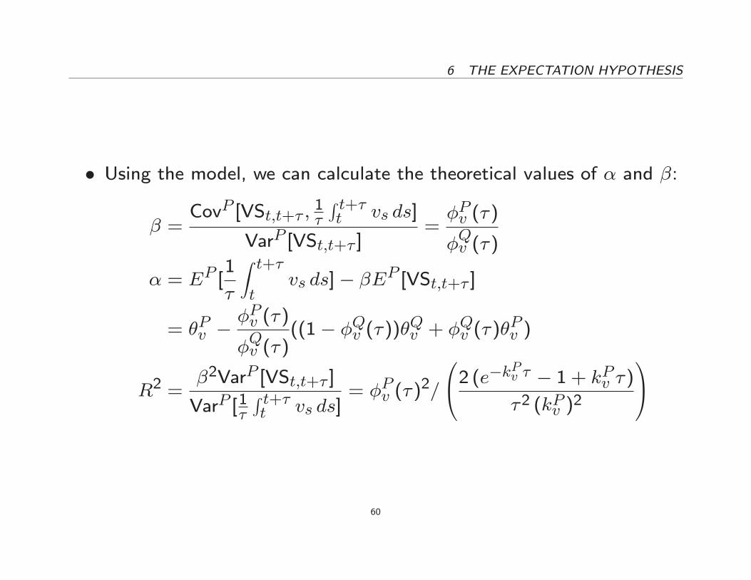
� Using the model, we can calculate the theoretical values of � and �:

� =CovP [VSt;t+� ;

1�

R t+�t vs ds]

VarP [VSt;t+� ]=�Pv (�)

�Qv (�)

� = EP [1

�

Z t+�t

vs ds]� �EP [VSt;t+� ]

= �Pv ��Pv (�)

�Qv (�)

((1� �Qv (�))�Qv + �Qv (�)�Pv )

R2 =�2VarP [VSt;t+� ]

VarP [1�R t+�t vs ds]

= �Pv (�)2=

0@2 (e�kPv � � 1 + kPv �)�2 (kPv )

2

1A

60


� When � ! 0, �(�) ! 1 and �(�) ! 0. Thus, for very short matu-

rities VS rates are e�cient and unbiased predictors of future realized

variances. This result is essentially due to the annualized realized vari-

ance, 1�R t+�t vs ds, converging to the spot variance vt, when � ! 0.

� When � ! +1, �(�)! kQv =k

Pv and �(�)! 0. Hence, for very long

maturities VS rates are ine�cient but unbiased predictor of future

realized variance. As kQv = kPv + 2�v and 2 is estimated to be

negative, kQv =k

Pv < 1.

� This suggests that VS rates tend to overestimate future RV.

61


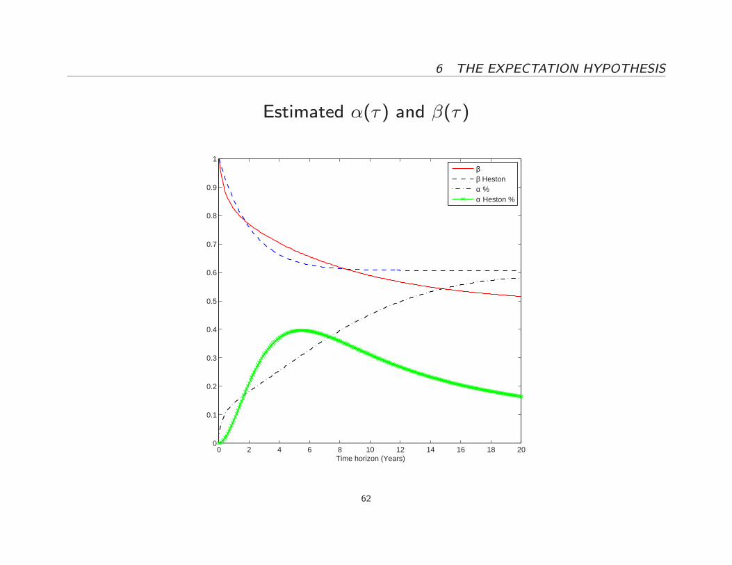
Estimated �(�) and �(�)

0 2 4 6 8 10 12 14 16 18 200

0.1

0.2

0.3

0.4

0.5

0.6

0.7

0.8

0.9

1

Time horizon (Years)

ββ Hestonα %α Heston %

62


� For the range of VS rate maturities in our sample (up to 2 years), �(�)decreases.

� Hence, predictions of future realized variances based on VS rates ap-pear to deteriorate quickly.

� When � = 2 years, R2(�) is about 70% in the general model.

63

7 SHORTING VARIANCE SWAPS?

7. Shorting Variance Swaps?

� As the ex-ante IVRP is negative, shorting VS generates a positivereturn on average.

� Moreover, in contrast to stock returns, volatility is partially predictablebecause it follows a persistent and mean reverting process.

{ For example, if today's volatility is high, it is likely that it willremain high in the near future, but eventually will revert to lowerlevels.

{ In that case, a sensible investment may be to go short in a long-term variance swap contract or \sell volatility," speculating thatlong-term future volatility will be lower than the current varianceswap rate.

64


� In order to examine the extent to which the large variance risk premiapotentially translate into economic gains, we consider a simple but

relatively robust trading strategy involving VS.

{ The strategy is to short the VS contract only when the expected

pro�t is large enough and precisely n times larger than its ex-ante,

model-based standard deviation.

{ When n = 0, the VS contract is shorted as soon as the expected

pro�t is positive. When n > 0, the contract is shorted less often.

65


� As a benchmark, we consider the following trading strategy based onthe S&P500 index.

{ If at day t the VS contract with maturity t+� is shorted, we invest

$1 in the S&P500 index and liquidate the position at day t+ � .

{ The actual return is computed using S&P500 index prices. This

buy-and-hold strategy is repeated for each day t in our sample.

66


� Shorting VS appears to be signi�cantly more pro�table than investingin the S&P500 index, over the same time horizons.

� Sharpe ratios from investing in VS are nearly uniformly and signi�-

cantly increasing in the threshold n.

� The only exception is from shorting the 2-month VS contract in the

out-of-sample period, as such positions su�ered large losses during the

Fall of 2008.

67


Estimated Returns of the Strategy

97 98 99 00 01 02 03 04 05 06 07 08 09 10−60

−40

−20

0

20

40

60

Year

12m

−R

etur

n %


S&P500Int−RateShort VS

68


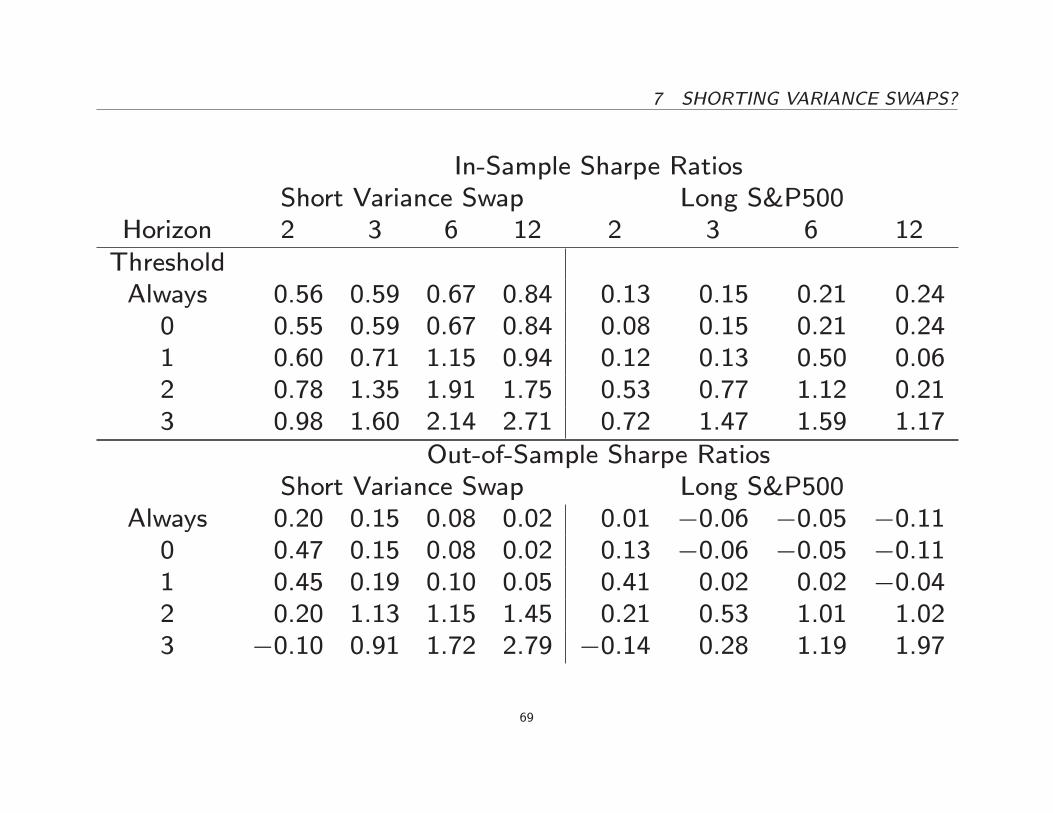
In-Sample Sharpe RatiosShort Variance Swap Long S&P500

Horizon 2 3 6 12 2 3 6 12ThresholdAlways 0.56 0.59 0.67 0.84 0.13 0.15 0.21 0.240 0.55 0.59 0.67 0.84 0.08 0.15 0.21 0.241 0.60 0.71 1.15 0.94 0.12 0.13 0.50 0.062 0.78 1.35 1.91 1.75 0.53 0.77 1.12 0.213 0.98 1.60 2.14 2.71 0.72 1.47 1.59 1.17

Out-of-Sample Sharpe RatiosShort Variance Swap Long S&P500

Always 0.20 0.15 0.08 0.02 0.01 �0.06 �0.05 �0.110 0.47 0.15 0.08 0.02 0.13 �0.06 �0.05 �0.111 0.45 0.19 0.10 0.05 0.41 0.02 0.02 �0.042 0.20 1.13 1.15 1.45 0.21 0.53 1.01 1.023 �0.10 0.91 1.72 2.79 �0.14 0.28 1.19 1.97

69


� The losses during 2008 re ect jump and volatility risk that short po-sitions are carrying, but they are smaller than the losses from the

buy-and-hold S&P500 strategy.

� Long positions in the S&P500 generate substantial more volatile re-turns.

� Interestingly, shorting VS does not appear to su�er from the \pick-

ing up nickels in front of steamroller" syndrome during the period

we looked at, despite the inclusion out-of-sample of the 2008{2009

�nancial crisis.

70


� Shorting VS provides some diversi�cation bene�ts as the correlationsshow:

In-Sample Out-of-SampleS&P500 Int-Rate Short VS S&P500 Int-Rate Short VS

2-month Returns 2-month ReturnsS&P500 1.00 0.09 0.57 1.00 �0.31 0.63Int-Rate 0.09 1.00 �0.01 �0.31 1.00 �0.25Short VS 0.57 �0.01 1.00 0.63 �0.25 1.00

12-month Returns 12-month ReturnsS&P500 1.00 0.05 0.30 1.00 �0.64 0.91Int-Rate 0.05 1.00 �0.01 �0.64 1.00 �0.54Short VS 0.30 �0.01 1.00 0.91 �0.54 1.00

71

8 CONCLUSIONS

8. Conclusions

� Signi�cant and time-varying jump risk component in VS rates.

� The term structure of variance risk premium is negative and generally

downward sloping.

� Going short long-term VS contracts is more pro�table on average than

going short short-term contracts.

� Variance risk premia due to negative jumps exhibit similar features inquiet times but have an upward sloping term structure in turbulent

times.

� Short-term variance risk premia mainly re ect investors' \fear of crash,"rather than the impact of stochastic volatility on the investment op-

portunity set.

72

Documents

The Term Structure of Variance Swaps, Risk Premia and the ...The Term Structure of Variance Swaps, Risk Premia and the Expectation Hypothesis ... which in the case of the S&P500 is