llanaurapll ll!ries In Finance and Eaana•I• Monograph 1989-1

The Stripping of U.S. Treasury Securities

By Miles Livingston and Deborah Wright Gregory

Salomon Brothers Center for the Study of Financial Institutions

Leonard N. Stern School of Business New York University

SALOMON BROTHERS CENTER FOR THE STUDY OF FINANCIAL INSTITUTIONS

Director: Arnold W. Sametz

Associates Program The Associates consist of leading members of the financial

community who are both knowledgeable and supportive of the activities and publications of the Salomon Brothers Center for the Study ofFinancial Institutions. These special friends in the financial community work with us to further interaction of financial executives and research faculty, and to ensure stability of funding for research at the Center.

Corporate Associates

Chicago Board Options Exchange, Inc.

The Equitable Life Assurance Society of the United States

Merck & Co., Inc. National Association of

Securities Dealers, Inc. Pfizer Inc. The Prudential Foundation

Associates

American Stock Exchange The Guardian Life Trust Hull Trading Co. Interactive Data Corporation Institute Bancario San Paolo di

Torino New York Cotton Exchange New York Stock Exchange Nomura Research Institute

(America) Inc. Quick Corp. Securities Industry Automation

Corporation Yamaichi Research Institute

Anonymous Associates

LEONARD N. STERN SCHOOL OF BUSINESS Dean: Richard R. West

NEW YORK UNIVERSITY President: John Brademas

MONOGRAPH SERIES IN FINANCE AND ECONOMICS Monograph l 989-1

The Stripping of U.S. Treasury Securities

By Miles Livingston and Deborah Wright Gregory

Miles Livingston is a professor at the Graduate School of Business Administration, University of Florida in Gainesville.

Deborah Wright Gregory is a professor at the University of Georgia.

The authors would like to thank the following for their comments and assistance: J. Walter Elliott, Haim Levy, Frances Sirianni of Salomon Brothers, Bill Emerson and Deborah Whitemore of Merrill Lynch, Tim Hart, Thomas Kluber, Michael Ryngaert, and David Brown.

MONOGRAPH SERIES IN FINANCE AND ECONOMICS

Editor: Anthony Saunders Managing Editor: Mary Jaffier

The Monograph Series of the Stem School of Business of New York University specializes in the publication of original studies in the fields of finance and economics. It provides an outlet for manuscripts which are too long and too broad in scope for the scholarly journals or of too great depth for the business periodicals. The submission of manuscripts in these fields is solicited.

For subscription rates and single copy order, see inside back cover.

The Monograph Series is published by the Salomon Brothers Center for the Study of Financial Institutions at the Leonard N. Stem School of Business of New York University. Editorial offices are located in 1307 Merrill Hall, 90 Trinity Place.

Sponsoring Subscribers

Bankers Trust Company Bernstein-Macaulay, Inc. The Chase Manhattan Bank,

N.A. Chemical Bank Citibank, N.A. CoreStates Financial Corp. Cowen & Company The Dreyfus Corporation The Equitable Life Assurance

Society of the United States Exxon Corporation

The Guardian Life Insurance Company of America

Manufacturers Hanover Trust Company

Metropolitan Life Insurance Co111pany

Morgan Guaranty Trust Company

Phibro-Salomon, Inc The Prudential Insurance Co. of

America Salomon Brothers, Inc

Table of Contents

I. Introduction 1

II. The Market for Zero Coupon Bonds 4

III. Pricing of Bonds in a Nontax Perfect Market 11

IV. Taxation of Bonds 16 Different Tax Treatments 19

Pricing Conditions 24

Equilibrium Conditions 26

V. The Value of Strips Versus the Underlying Bonds 28

VI. Examples of the Profits from Stripping 33

VII. Classification of Stripped Securities 50

VIII. Rebundling 51

IX. Stripping and the Pricing of Underlying Bonds 55

X. Coupon Effects 58

XI. Conclusion 60

Appendices 61

References 65

Copyright 1989 New York University

I. Introduction

Beginning in September 1982, the practice of stripping U.S. Treasury securities developed. As of mid-1988, about $80 of par value of U.S. Treasury securities was in stripped form. When stripping first started, a financial institution would purchase a block of U.S. Treasury securities, place these securities in trust, and then sell claims on the individual cash flows. To illustrate, if a 10-~ear bond with 20 semi-annual coupons is stripped, the underlying bond is resold as 21 zero coupon bonds, each of which trade separately in the secondary market.

In order to expedite stripping, the U.S. Treasury in 1985 declared some Treasury securities eligible to be stripped through the Fed­eral Reserve book entry system; the resulting securities are called STRIPS (which stands for Separate Trading of Registered Interest and Principal of Securities). In 1987, the Treasury began to allow strips to be rebundled into the original underlying securities. Stripping and rebundling through the Treasury program involves essentially zero cost and consequently stripping and rebundling is currently dominated by the Treasury STRIPS program.

Active stripping of U.S. Treasury securities became prevalent after July 1982 following a change in the tax treatment of original issue discount bonds. 1 The new tax law changed the timing of tax liabilities for buyers of stripped bonds, which are treated as original issue discount bonds for tax purposes. This paper show that the 1982 tax law change created an opportunity for financial institutions to profit from stripping U.S. Treasury securities.

We will show that the fair market value of a portfolio of the individuals strips will differ from the value of a whole bond due to differences in the tax treatments. The tax treatment of the strips can be more favorable than the tax treatment of the underlying bond for some term structures. Specifically, underthe post-July 1982 law, in a perfect market with all securities fairly priced, bonds can have a greater value repackaged

1Before July 1982, original issue discounts from par were linearly amortized. After this date, the discount was amortized by the constant yield method, described in detail in Section IV of the monograph. With the constant yield method, the initial amortization is small and grows as time elapses. The tax treatment for corporate issues is symmetric. See Pyle (1981) for a discussion of the corporate tax advantages of original issue discount bonds.

as strips for rising term structures. Institutions that strip bonds can make an immediate, risk-free arbitrage profit. Thus, the tax law change and the resulting profits appear to have provided an incentive for underwriters to strip U.S. Treasury securities.

The tax advantage from stripping will depend upon the tax treatment of the underlying bond. Although the tax treatment of the underlying bonds has changed several times since July 1982, we will show that a net advantage can still exist under each tax treatment to strip premium, par, and discount bonds for rising term structures. The advan­tage of stripped securities increases (1) as the slope of the yield curve increases, (2) as maturity increases, (3) as the tax rate increases, and (4) as the level of interest rates increase.

Under the Treasury STRIPS program both stripping and rebundling occur. This has an important impact upon the equilibrium pricing of underlying bonds. That is, the market value of an underlying bond must equal the higher of the value of a nonstrippable bond or a portfolio of STRIPS plus the value of an option to exchange bonds for STRIPS and vice versa. Thus, a strippable bond must be worth more than a portfolio of nonrebundable STRIPS. It follows that the Treasury is better off to issue strippable coupon-bearing bonds than to issue zero coupon bonds.

Since re bundling of Strips began in mid-1987, we have observed stripping ofunderlying bonds, shortly followed by rebundling of these same bonds. This unusual phenomenon is shown to occur because of the different taxation of STRIPS and underlying bonds and shifts in the level of the yield curve. For rising yield curves, some bonds may be worth more as strips because of taxes. For slightly lower levels of yields, these strips may then be worth more as repackaged underlying bonds because of the tax differences between strips and underlying bonds. As the level of yield changes, arbitragers strip or rebundle to keep prices in line.

The taxation of strips significantly alters the coupon effect upon yield to maturity. For rising term structures, strips will have higher yields than par bonds.

For many years, the finance literature has discussed the problem of how investors can immunize against interest rate risk.2 An immunizertries to lock in a fixed return over a given horizon. Ideally, zero coupon bonds should be used to immunize because there is no problem of reinvesting coupons. Quite surprisingly, original issue zero coupon bonds have been relatively scarce. Consequently, most of this immunizing

'See Bierwag ( 1977 and 1987), Bierwag and Kaufman (1977), Fisher and Weil (1971), Hopewell and Kaufman (1973),Redington (1952), and Samuelson (1949).

2

literature has examined immunizing strategies using coupon-bearing bonds; these strategies can be costly and difficult to implement. The problem of immunizers has been made easier in recent years by an increase in the supply of zero coupon bonds, created through the practice of stripping U.S. Treasury securities.

This monograph analyzes stripping in a perfect market. If market imperfections exist, some people believe the demand for zero coupon securities will increase.3 According to this segmented market view, some investors (e.~ .. tax-free investors or immunizers) may be willing to pay prices above perfect market values set by the marginal investor, tending to increase the value of the stripped securities. The segmented market view does sot explain the sudden emergence of coupon stripping immediately after the tax law changed in 1982. This sudden shift is documented in Table 3 in the text. Under the segmented market view, the incentive to strip underthe old tax law was at least as great as under the post-July 1982 law. Yet there was no stripping before July 1982. Thus, the segmented market view cannot explain the sudden emergence of stripping in mid-1982, immediately after the tax law changed. This suggests that the segmented market view cannot by itself explain stripping, although market imperfections might add to the incentives to strip bonds under the post-July 1982 tax law.

Since mid-1987, Treasury STRIPS have been rebundlable, meaning that arbitrage will force the prices of STRIPS and underlying bonds to be in line with each. Thus, if a particular group of investors bid up the prices of STRIPS, arbitrage between markets would eliminate any disparities. With stripping and rebundling, the STRIPS market cannot be segmented.

3See Kanemasu, Litzenberger, and Rolfo (1986).

3

IL The Market for Zero Coupon Bonds

Zero coupon bonds are very attractive investment vehicles for investors who are immunizers, such as pension funds and insurance companies. These bonds allow the locking-in of a terminal value, which is highly desirable for these investors, as it eliminates the reinvestment risk associated with coupon-bearing bonds. Given the likelihood of sizable demand for zeros by immunizers, it is somewhat surprising that relatively few zero coupon bonds have been issued (see Kaufman, 1973).

Apartment from Treasury bills, the U.S. Treasury has not issued zeros, although the tax treatment for Treasury zeros used to be attractive to buyers. Between 1969 and 1982, the U.S. tax law specified that U.S. Treasury securities issued at a discount would tax the discount as regular income at maturity. Thus, the tax would be postponed until maturity. Nevertheless, the U.S. Treasury chose not to issue long-term dis­count securities.

A major explanation for the lack of corporate zeros probably lies in the tax laws (see Livingston, March 1979). For bonds originally issued at a price other than par, a special tax treatment has applied. Prior to June 1982, for corporate bonds originally issued at a discount below par, the discount was required to be amortized on a straight line basis over the bond's life as an addition to taxable income. For example, ifa ten year zero coupon bond with $1 OOparvalue was issued at$50, the buyer was required to add $5 (i.e., (I 00-50)/10=5) to taxable income for each of 10 years of the bond's life. Thus, the buyer would have to pay taxes each year for ten years before receiving a positive cash inflow at maturity. The present value of the tax liabilities would tend to be high relative to the present value of par, implying relatively low values forthese zeros. Under some circum­stances, the present value of the tax liabilities could exceed the present value of par, implying that the zero coupon bond would have no value.

The tax treatment of an original issue discount security for the issuer is symmetric with the tax treatment for the buyer. Before July 1982, corporations issuing zeros would be able to amortize the discount from par on a straight line basis as a deduction from taxable income. If the corporate tax rate is higher than the tax rate of the buyer, there may be situations where issuance of zeros may be advantageous for both parties. Tax con­siderations may have motivated the popularity of corporate zeros during the late 1970s and early 1980s (see Pyle, 1981).

4

Besides tax considerations, other factors have provided ob­stacles to issuance of zero coupon corporate bonds (see Livingston, March 1979). A big obstacle is the problem of default. With coupon-bearing bonds, the issuing corporation has to regularly pay semiannual coupons. Otherwise, there is default and possible bankruptcy. The payment of regular coupons serves as a signal of financial strength. With zero coupon securities, default on cash flows can occuronly at maturity. The bondhold­ers would find it desirable to design some protective covenants to ensure the issuer's financial well-\Jeing. The method for doing this is not clear and may be an obstacle of issuance of zero coupon bonds.

Table I shows the yearly issuance of corporate zeros since 1981. This is compared to the issuance of all types of corporates.

In July 1982, the tax law fororiginal issue discount securities, which includes both corporate and Treasury zeros, changed to what we shall call the constant yield method. Under this method (described in detail below), the amount of amortization starts at a low level and increases geometrically. Figure I compares amortization by linear amortization and by the constant yield method. Under each method the entire discount is amortized. But with linear amortization, the early amortization is rela­tively large, clearly a disadvantage from the buyer's viewpoint.

We will show that the tax law change in July 1982 signifi­cantly increased the value of original issue zero coupon securities for rising term structures compared to the old tax law. This new law motivated financial institutions to strip U.S. Treasury securities, because the value of a portfolio of strips could now exceed the value of an underlying bond due to the different tax rules applicable to each type of security.

Table 1. Corporate Zeros.

Par Value of Par Value of Zeros Issued Number New Corporate

Year ($Millions) of Issues Bonds ($ Millions)

1981 2,146 20 45,092 1982 8,645 118 54,076 1983 325 39 68,495 1984 1,887 53 109,683 1985 480 95 203,500 1986 500 30 355,293 1987 432 12 232,969

Sources: Zero Coupon Bonds from IRS Publication l 212 Corporate Bonds from Treasury Bulletin

5

FIGURE 1

Constant Yield Method

(f) 0'"------------------' ([)<( PAR,---------------""71 ro Linear Amortization

6

0'"------------------' ISSUE DATE

MATURITY

The following example in Table 2 shows how the individual components of stripped securities are priced. To illustrate, a ten year bond with 20 semiannual coupon payments and one par value is decomposed into its 21 parts, each of which trades separately. This example assumes a I 0 year bond which is selling at its par of$ J ,000. The bond has a semi­annual coupon of$50. The term structure is flat. The bond is decomposed into parts worth $1,000. Later examples will show that with a nonflat term structure, the portfolio of stripped securities can have a different value than the underlying bond because of different tax treatments.

Table 2. Example of Stripping for Flat Term Structure

$1,000 ten-year par bond is stripped. Current price = $1,000 Par Value= $1,000 Semiannual Coupon = $50

Time to Maturity

Years Payment

.5 $ 50 l.O 50 l.5 50 2.0 50 2.5 50 3.0 50 3.5 50 4.0 50 4.5 50 5.0 50 5.5 50 6.0 50 6.5 50 7.0 50 7.5 50 8.0 50 8.5 50 9.0 50 9.5 50

10.0 1,050

Total

Price of Stripped

Component

$ 47.62 45.35 43.19 41.14 39.18 37.31 35.53 33.84 32.23 30.70 29.23 27.84 26.52 25.25 24.05 22.90 21.81 20.78 19.79

395.73

1,000.00

7

The incidence of stripping over time is chronicled in Table 3. Stripping began in September 1982, two months after the change in the tax law in July 1982, and has continued since then. Originally, stripping was carried out by financial institutions that bought up blocks of Treasury securities, put them into trust, and sold claims on the parts. The first two big strippers were Merrill Lynch who created TIGRS (i.e., Treasury Investment Growth Receipts) and Salomon Bros. who created CA TS (i.e., Certificates of Accrual on Treasury Receipts).

Month

1982 1983 1984 1985 1986 1987

Table 3. Stripping of U.S. Treasury Securities

Par Values of Underlying Bonds ($Millions) End-of-Year Cumulative Totals

CATS& TIGRS TRs* STRIPS

1,673 4,901

18,174 19,830 12,179 22,952

32,444 44,774**

* TR stands for Treasury Receipts. See article by Kluber and Stauffacher ( 1987). ** See Table 12 for additional information on STRIPS.

The motivation for stripping was the opportunity to resell the portfolio of stripped securities for a higher price than the underlying bonds. We will show that the portfolio of strippeg securities may have a higher value than the underlying securities in a perfect market for rising term structures. The difference in value is caused by the difference in tax treatments between the underlying bond and the stripped securities, which are taxed as original discount securities.

In practice, market imperfections created positive costs to stripping. First, the cost of setting up trust accounts was positive, although not relatively large. Second, the stripping institution had to find buyers for the strips. This required a marketing network. Third, a stripping institution bore the risk of interest rate changes from the time that the underlying bond was purchased until the time that all the strips were sold. This risk could be reduced considerably by hedging with interest rate futures contracts.

8

Since 1985, the U.S. Treasury has allowed stripping through the Federal Reserve book entry system. The resulting securities are called STRIPS and as seen in Table 3 have come to dominate the market for stripped securities. This form of stripping is less costly because special trust accounts are not necessary.

Traditionally, Treasury bonds have been callable during the last five years of their lives. This call feature makes stripping more complicated. The callable parts of a bond are stripped as one package; this package includes the last IO semiannual coupons and the par value. For many investors, the last five years of callable cash flows were not a very attractive purchase. Recent issues of strippable long-term Treasury bonds have been noncallable to expedite stripping.

By issuing noncallable long-term bonds which can be easily stripped, the Treasury has probably reduced its interest costs. This can be explained as follows: If an underlying security can be decomposed into a portfolio of securities worth more in stripped form, there will be incentives for strippers to arbitrage between the markets by buying the low priced underlying security and selling the high priced stripped securities. This arbitrage will tend to force the price of the underlying security to be no lower than the price of the portfolio of strips, if the strips are worth more. In fact, a strippable bond must be worth the higher of the value of a non­strippable bond or strips plus the value of an exchange option.

If prices were not in equilibrium, the Treasury might have an incentive to issue zeros. But, if prices are in equilibrium, the underlying bond would not sell for less than the value of the stripped securities. Consequently, the Treasury can be no worse off by issuing only coupon­bearing bonds, provided that the underlying bonds can be easily stripped by book entry.

In 1987, the Treasury began to allow strips to be re bundled into underlying bonds. Thus, under current rules, underlying bonds can be stripped and strips rebundled repeatedly. An underlying bond which can be stripped and then re bundled repeatedly must be worth more than a bond which can only be stripped only once. Rebundling has further raised the value of the underlying bonds and reduced Treasury interest costs.

Apart from Treasury bills, the U.S. Treasury has never issued zero coupon securities. Prior to 1982, original issue Treasury discount securities had a special tax treatment. The discount would be taxed at maturit)'. as regular income and would not have to be amortized. From a tax viewpoint, Treasury zeros prior to 1982 would appear to be relatively attractive compared to corporate zeros, which would have to be amortized. Yet no Treasury zeros were issued, suggesting that some other considera­tions discouraged issuance.

9

One such consideration would be the question raised regard­ing measurement of the level of the national debt, if zero coupons were issued by the Treasury. Several methods for measurement seem plausible. One possibility might be to count the par values of Treasury zeros as part of the national debt; this treatment would result in reduced annual interest expenses but a much larger debt. This strategy would reduce current budget deficits (because of lower current interest cost), but raise the national debt. Conceivably, issuance of zeros might be used by some ad­ministrations to window-dress the budget deficit. A second possibility might be to count the original issue price of zeros as part of the debt and allocate the difference between par and issue price as annual interest. Since the interest doesn't have to be paid until maturity, funds would probably have to be set aside to pay interest, defeating the whole purpose of issuing zero coupons.

Stripping of coupon-bearing corporate bonds has not oc­curred. The reason may be concern about the question of default. If a corporate bond is stripped and the corporation then defaults, the stripping institution probably would have some contingent liability to the buyer of the stripped securities. The present value of contingent default liabilities could easily outweigh the current profit from stripping resulting in much lower or potentially negative profits from stripping.

10

III. Pricing of Bonds in a Nontax Perfect Market

This section will discuss the pricing of bonds in a perfect market with no taxes. Then the implications of taxation can be more readily discussed in the ne~t section. In a perfect market there will be (I) no transaction costs, (2) no call features, (3) no default, (4) unrestricted shortselling, and (5) no taxes. Unrestricted shortselling means that the seller can use the proceeds, implying that default by the shortseller is impossible.

A zero coupon bond pays only a par value to the buyer. The cash flows are shown in Table 4. Let the spot interest rate for n periods be denoted by R(n). Ann period zero coupon bond, paying $1 at time n, has a present value of D(n) where

1 D(n) = [I+ R(n)]" (3.1)

A coupon-bearing bond pays periodic coupons and a par value at maturity. The price of an n period coupon-bearing bond with coupon of c and par value ofF is P and should be the present value of these cash flows, where

c c c +F P=--+ +···+---

l+R(l) [I+R(2))2 [l+R(n)]" (3.2)

This can be expressed as

P = cD(l) + cD(2) + ... + (c+F)D(n) (3.3)

That is, a coupon-bearing bond is a portfolio of zero coupon bonds. It will be convenient to write the present value of an n period annuity of $1 per period as A(n), where

I I A(n)= -- +--- +···+---

l+R(l) [l+R(2)]2 [l+R(n)J" (3.4)

A(n) = D(l) + 0(2) + ... + D(n) (3.5)

II

Using this expression for the value of a $1 annuity, the price of a coupon bearing bond can be expressed as

P ; c A(n) + F D(n) (3.6)

This expression indicates that there is a linear relationship between price and coupon for a given maturity and is shown graphically in Figure 2. The slope is A(n), the present value of an annuity. The vertical intercept is F D(n), the price of a zero coupon paying F at maturity of n.

Table 4. Bond Cash Flows

Zero Coupon Bonds Points in Time 0 n

-D(n) $1 purchase par

price value

$ Annuit Points in Time 0 2 n

-A(n) $1 $1 $1 purchase

price

Coupon-Bearing Bond Points in Time 0 2 n

-P $c $c $c+$F purchase COUJ?OilS coupons

price and par value

12

FIGURE 2

PRICE LINEAR FUNCTION OF COUPON PRICE

2(f) 2o 2z WO 0:: co Q_

PARl-----lf----~~~~~~

f--Z ifJ ::>O oz uo if) co Ci ZER

COUPON BOND

0 COUPON OF

PAR BOND

COUPON

13

The yield to maturity for coupon c and maturity n is the rate y(c,n) satisfying

P= I c . + __ F __ _ j=I [l+y(c,n)]J [l+y(c,n)]"

(3.7)

P can also be expressed in terms of spot (zero coupon) interest rates (RU)'s),

n

L: j=l

c F -~-·+ -~ = [I+RU)]J [+R(n)J"

n c F L: i+ n i=I [l+y(c, n)] [I+y(c, n)]

(3.8)

This indicates that the yield to maturity is a polynomial function of the spot interest rates. In general, it is not possible to express the yield to maturity as an explicit function of the spot interest rates. An exception is the case of par bonds. Let y(par,n) be the yield on a par bond with maturity n. Then by setting price equal to par and solving for y (par, n), we find that

I - D(n) y(par, n) = A(n) (3.9)

An extensive literature examines the relationship between the spot rates and yield to maturity for a particular maturity. If the spot rates are all equal, the yield to maturity is the same for n period bonds of all coupon levels. This is illustrated in Figure 3. If the spot rates increase monotonically with maturity, for n period bonds the yield to maturity is high for low coupon bonds and decreases as the coupon increases. For a zero coupon bond, the yield to maturity will be then period spot rate R(n). As the coupon increases, the other n-1 spot rates affect yield to maturity. Since these shorter maturity spot rates are lower than R(n), adding them to the average will tend to reduce yield to maturity.

In summary, coupon bearing bonds are essentially portfolios of zero coupon bonds in a world with no taxe&. If there are personal income taxes on bonds, the portfolios are more complex, as discussed in the next section.

14

FIGURE 3

COUPON EFFECTS

YIELD

POSITIVE

NEUTRAL

NEGATIVE

0 COUPON

15

IV. Taxation of Bonds

This section will discuss the tax treatment of bonds. For all bonds, coupons received are taxed as regular income. Many bonds sell at discounts below par or premiums above par. The tax treatment of discounts or premiums from par will depend upon whether or not the bond was originally issued at par. In most cases, bonds are issued at par. If so, any subsequent discount or premium from par is considered to be a gain for discounts or a loss for premiums.

For bonds originally issued at a discount, the discount must be amortized as income over the bond's life. For income tax purposes, stripped securities are considered original issue discount securities. Prior to July 1982, discounts from par for original issue discount securities were amortized on a straight line basis. In July 1982, the tax law for original issue discount securities was changed to the constant yield method for both issuers and buyers. Under the constant yield method (explained in detail shortly), the amortized amount increases over time, resulting in smaller deductions in the early years and bigger deductions in the later years compared to the straight line method. For bond purchasers, the present value of the tax liabilities is lower under the constant yield method than under linear amortization making the market value of a bond higher, ceteris paribus.

For bonds originally issued at par, the taxation of subsequent discounts and premiums from par in the resale market is complicated because discounts and premiums from par in the resale market are taxed asymmetrically and because the tax treatment has been changed for capital gains. We will examine bond prices for four hypothetical tax treatments. For each case, stripping may be profitable depending upon the term structure, maturity and coupon level. In the discussion below these hypothetical tax treatments are compared with the actual tax law since 1982. These tax treatments closely correspond io actual tax treatments of underlying bonds in the period after July 1982 as shown in Table 5.

We will make the following assumptions: (I) no transactions costs, (2) noncallable bonds,(3) nodefaultrisk,(4) unrestrictedshortselling, and (5) the tax rate of the marginal investor clears the market. Several situations fit this assumption: (I) all investors in the same tax bracket, and (2) a progressive system. Equilibrium in the progressive system is shown in Figure 4. Note that investors in low tax brackets (below the bracket of

16

the marginal investor) receive a windfall gain because their after-tax return is higher than the after-tax return of the marginal investor. For example, assume that the marginal investor has a 50% tax rate and the before-tax (1 period) interest rate is 10%. The extra5% is a windfall gain to the tax-free investor. In a perfect market, the tax-free investor would never be willing to accept less than 10% rate of return.

Table 5. Tax Treatments Applicable for Various Time Periods for Bonds

Originally Issued at Par.

Time Period

July 1982 - July 1984

Discount Bonds

Issued Before July 1984

Issued After July 1984

July 1984 - December 1986 January 1987 -

Treatment (1) Treatment (I) Treatment (2)

NIA Treatment (2)* Treatment (2)*

Time Period

July 1982 -

Treatment (I) Treatment (2) Treatment (3) Treatment (4) N/A

Premium Bonds

Issued Before Issued After September27, 1985 September27, 1985

Treatment (3)** Treatment ( 4)

Capital gains tax treatment Regular income tax on gains and losses Linear amortization Constant yield method Not applicable

*For bonds issued after July 1984, bondholders have the option of amortizing the discount over the bond's life. This might be advanta­geous if their tax rate increases over time.

** For investors with a constant tax rate over time, linear amortization would be preferable to a capital loss (Treatment (1 )). If the tax rate will be quite high at bond maturity, a capital loss might be advantageous.

17

FIGURE4

EQUILIBRIUM INTEREST RATE WITH PROGRESSIVE PERSONAL TAXES

INTEREST RATE

EQUILIBRIUM

TAXABLE INTEREST - - - - - - - - - -

RATE

TAX-FREE INTEREST....._ ____ _,....

RATE TAX- FREE INVESTORS

18

SUPPLY CURVE: BUYERS OF BONDS

DEMAND CURVE: ISSUERS OF BONDS

$

Notation. We will use the following notation: R(n) = the equilibrium after-tax (or tax-free) zero coupon

discount rate (spot interest rate) for funds received at time n.

t = tg = c = F = y(c, n) =

D(n) =

A(n) =

tax rate on regular income capital gains tax rate bond coupon par value the yield to maturity for a bond with coupon c and maturity n that is taxed by the constant yield method the price of an n-period tax-free zero coupon bond with $1 par value. D(n) = l/(l+R(n))" the price of an annuity paying $1 tax-free per period

" for n periods. A(n) = 2: (I +RG))"i ._, HG, n) = for the constant yield tfiethod, the time j hypotheti­

cal price of a bond maturing atn, assuming the bond is held to maturity and the yield remains constant. HG, n) is often called the "basis" for tax purposes. The basis is described in detail in the Appendix.

Different Tax Treatments

(1) Capital Gains Tax Treatment. Table 6 shows the cash flows resulting from holding a bond under this tax treatment. Pg equals the price of a bond assuming that discounts from par represent a capital gain, and premiums above par represent a capital loss at maturity. The gain or loss will be taxed at the special capital gains tax rate, tg. This case describes the tax treatment of all discount bonds for the tax period from July 1982 to July 1984. For the tax period July 1984 through December 1986, this case applies to all discount bonds issued before July 18, 1984. Beginning in 1987, gains and losses are taxed at regular income rates; case (2) below applies. See Table 5.

The price of a bond subject to the capital gains tax treatment should be the present value of the after-tax cash flows discounted at the after-tax term structure.

Pg= " c(l - t) F 2:---j + " i=' [l+RGJJ [l+R(n)]

tg(F - Pg) [l+R(n)]"

= cA(n) + FD(n) - tg(F - Pg) D(n)

(4.1)

(4.2)

19

Table 6. Cash Flows from Bonds

Case (1) CaQital Gains Tax Treatment Points in Time 0 I 2 n

-Pg c(l-t) c(l -t) c(l -t) + F purchase after-tax coupons par value

price -(F - Pg)tg

capital gains

tax at rate tg

Case (2) Regular Tax Rate on Gains Tax Treatment Points in Time 0 I

-Pt c(l - t)

purchase after-tax price

2

c( I - t)

coupons

Case (3) Points in Time

Linear Amortization

0 2

-Pa c(l - t) c(l - t) purchase after-tax coupons

price Amortization: -(F - Pa)t -(F - Pa)t of discount n ti

or premium

Case (4) Constant Yield Method Points in Time 0

-Py c(l - t) purchase after-tax

price Amortization: -t[H(I, n)-

H(O, n)]

H(j, n) is the basis at time j. t is the tax rate on regular income. tg is the capital gains tax rate.

20

2

c(l - t) coupons

-t[H(2, n)- ...

H(I, n)]

n

c(l - t) + F par value

-(F - Pt)t

capital gains tax at regular

tax rate

ti

c(l - t) + F par value

-(F - Pa)t n

n

c(l - t) + F par value

-t[F- H(n-1, n)]

Solving for PG and replacing D(n) for [I +R(n)l" and A(n) for the present value of an annuity results in

p _ cA(n)(l - t) + F(l - tg) g - I - tg D(n)

This equation can be rewritten as

Pg = c [ A(n) (I - t) ] + F [ l - tgD(n)

(1-tg)] l - tgD(n)

Pg= c[Present Value of Annuity]+ F[Present Value of $1]

(4.3)

(4.4)

This expression indicates that the price of a bond taxed by the capital gains method is the coupon times the present value of a special type of annuity plus par times the present value of a dollar taxed as a capital gain. The relationship between coupon and price is shown graphically in Figure 5.

(2) Regular Income Tax on Gains and Losses. Pt equals the price of a bond assuming that discounts and premiums are gains and losses taxed at maturity at the regular income tax rate t. For the tax period, July 1984 through December 1986, this was the usual tax treatment for bonds issued on or after July 18, 1984.4 Beginning with the tax year 1987 all capital gains are taxed at the regular income rate and consequently this case applies for purchase of all discount bonds beginning January 1987. See Table 6.

The price of a bond taxed by this method will be the present value of the after-tax cash flows discounted at the after-tax term structure.

Pt= c(l - t) A(n) + FD(n) - t(F - Pt) D(n)

Solving for Pt

Pt= c(I - t) A(n) + F(l - t) D(n) I - tD(n)

(4.5)

(4.6)

(3) Linear Amortization. Table 6 shows the cash flows for a bond purchased under this method. Pa equals the price of a bond that amortizes the discount or premium linearly over the bond's life at the

4Technically, bondholders are required to amortize gains by the constant yield method. However, the bondholder can elect to postpone the payment of tax on the amortization until the bond is sold or until maturity. In general, postponing the tax payments will be better.

21

regular income tax rate. Individual investors have the option of electing this tax treatment for premium bonds.5

The price of a bond taxed by this method will be

Pa; c(l - t) A(n) + FD(n) - t(F - Pa) A(n)/n

Solving for Pa

Pa; c(l - t) A(n) + F[D(n) - tA(n)/n] 1 - tA(n)/n

Pa; c(l - t) A(n) + F[D(n) - tA(n)/n] 1 - tA(n)/n 1 - tA(n)/n

; c[Present Value of an Annuity]

+ F[Present Value of Par]

(4.7)

(4.8)

(4.9)

(4.10)

(4) ConstantYieldMethod. Table 6 shows the cash flows that apply for a bond purchased under this method. Py equals the price of a bond which amortizes discounts and premiums on a constant yield basis over the bond's life. The regular income tax rate t applies. According to the constant yield method, the yield to maturity at time of purchase is im­plicitly assumed to be constant over the bond's life. Each period's gains or losses represent the tax liabilities for a discount bond or the tax deductions fora premium bond assuming the bonds were held to maturity. Original issue discount securities and stripped securities are taxed accord­ing to this method. In addition, for bonds originally issued at par after September 27, 1985 and subsequently trading at a premium, the premium must be amortized by the constant yield method.

The value of a bond using the constant yield method is the present value of the after-tax cash flows discounted at the after-tax term structure.

Py; c(l - t) A(n) + FD(n) - t I [HG, n) - HG - 1, n)] DO) (4.11) j=l

5See Livingston (September 1979) for a discussion of the taxation of premium bonds.

22

The basis is discussed in Appendix B. Equation (4.11) simplifies to6

Py = c(l - t) A(n) + FD(n) -

" D(j) t[y(c, n) F - c] I (l ( ))"·i+I

J=l + y C, Il (4.12)

This expression is shown graphically in Figure 5. For flat term structures, the price Py Of a bond taxed by the constant yield method is a linear function of price. As discussed later on, for rising (falling) term structures, there is a curveq relationship with the slope increasing (de­creasing).

By substituting c equals zero into equation (4.12), the price Z(n) of a stripped zero coupon bond with maturity n and face value of one dollar is

" D(j) (4.13) Z(n) = D(n) - ty(O, n) i~ (I + y(O, n))"·i+I

If the term structure is flat (that is, R(l) = R(2) = ... R(n) = R), Appendix A shows that the yield to maturity for all stripped securities is R/(l - t), which also is the yield on par bonds.

6ln general,

. ~ c F H(j, n) = t,1 (I + y(c, n))k + (I+ y(c, n))n-j

n-j+! c F

H(j-l,n)= ~ 1 (\+y(c,n))k + (l+y(c,n))n-j+!

. . (c+F) F y(c,n)F-c HU n) - HU-l n) = - + -

' ' (l+y(c,n))n-j+l (l+y(c,n))n-j - (l+y(c,n))n-j+l

23

FIGURE 5

PRICE

PAR 1.0

COUPON

24

Pricing Conditions

Define p-, P0, P' as the prices of discount, par, and premium

bonds. Then 7

Pa· < Py-< Pr <Pg· (4.14)

Pa0 = Py0 = Pt0 = Pg0 (4.15)

Pa+> Py+> Pt+> Pg+ (4.16)

These conditions are illustrated in Figure 5 and are used below in developing conditions when stripping is profitable. Equation (4.15) says that for par bonds all of the four tax treatments are identical because there are no discounts or premiums from par; only the coupon is taxed. Equation (4.14) compares discount bonds with the same coupon level. Prices will differ because of the tax treatments of the discounts. Linear amortization Pa· has the most unfavorable tax treatment because the discount from par is amortized rapidly and taxes must be paid sooner. The constant yeild method amortizes the discount, but not as fast as linear amortization. Consequently, some tax payments are postponed with the constant yield method. The regular income tax method postpones recog­nition of the discount until maturity. The capital gains method postpones the gain until maturity and has a reduced tax rate, and consequently is the most favorable tax treatment for discount bonds.

Equation ( 4.16) compares premium bonds. Premiums above par are deductions from income and result in tax advantages. Linear amortization is the most favorable tax treatment because the deductions from income and the tax savings occur rapidly. The constant yield method also amortizes deductions over the bond's life, but the deductions are not

7From Arditti and Livingston [2], Pg= [c(l - t) A(n) + F(l - tg)]/[l - tgD(n)] Pt= [c(l - t) A(n) + F(l - t)]/[l - tD(n)] Pa= [c(l - t) A(n) + F(D(n) - tA(n)/n] I [I - tA(n)/n] Since t > tg, Pr< Pg· and Pt+> Pg+. Since linear amortization results in quicker

amortization than the constant yield method. Pa·< Py· and Pa+> Py+. Since tax liabilities and deductions are realized over the bond's life for the constant yield method, and since the gains and losses are deferred until maturity for the regular income method, Py·< Pr and Py+> Pt+. Equations (4.14) and (4.16) follow directly from manipulating the above inequalities.

25

as rapid as for linear amortization. The regular income and capital gains methods postpone the deductions until maturity and are less favorable than amortization. The capital gains method has the lowest tax rate and therefore the smallest tax savings.

Equilibrium Conditions

If investors are given a choice of the method for taxation, they will choose the most favorable method, i.e., that minimizes the present value of taxes. It follows that equilibrium prices should be set by the most favorable tax treatment available to investors.

Since linear amortization can be elected by taxpayers for bonds issued before September 27, 1985 and since premium bonds are worth more under linear amortization, premium bonds will be valued by the linear amortization method in equilibrium. For discount bonds, linear amortization does not apply; prices will be determined by the capital gains rate method or regular income method, depending upon the point in time when the bond was purchased. The equilibrium pricing function will have two line segments as shown in the top of Figure 6.

For bonds issued after September 27, 1985, the constant yield method applies for premiums. For discount bonds, the regular income tax method applies after January I, 1987. For this combination of tax rules, equilibrium is shown in the bottom of Figure 6.

26

PRICE

PAR

FIGURE 6

EQUILIBRIUM PRICE vs. COUPON DISCOUNT BONDS TAXED BY CAPITAL GAINS METHOD PREMIUM BONDS TAXED BY LINEAR AMORTIZATION

Pg

C=O Cpar COUPON

PAR

DISCOUNT BONDS TAXED BY REGULAR INCOME METHOD

PREMIUM BONDS TAXED BY CONSTANT YIELD

Py

P,

Cpar

27

V. The Value of Strips Versus the Underlying Bonds

This section compares the value of stripped securities versus the value of the underlying bond for the four tax treatments described earlier. We will prove thatthe total value of strips under the post July 1982 tax law equals the value of a bond priced by the constant yield method, but only for a flat term structure. In general, the total value of the strips will not equal the value of the underlying bond. For rising term structures the fair value of the strips can be higher than the market value of the underlying bond for some coupon levels for each of the four tax treatments described earlier under the post July 1982 tax laws. Term structures have been rising since July 1982.

A. Comparison of Bonds Taxed by the Constant Yield Method Versus the Portfolio of Individual Strips. Consider an n-period bond with coupon c. Assume an investor buys a portfolio of individual stripped securities with the same pre-tax cash flows as a particularn-period coupon-bearing bond. The portfolio of individual strips should have a market value of V, where

' V = c I ZU) + F Z(n) (5.1) }=l

Substituting for the values of Z from equation (4.13) we have

i D(i) V = c I DU) - ct I y(O, j) I (I (O '))i-;"

J=l J=l !=l + y ,j

' DU) + FD(n) - Fty(O, n) I ( 1 (O ')) _. 1 j=J +y ,j nJI'

(5.2)

28

Algebraic manipulations indicate that

[ " . " . i D(i) ]

V - Py= ct I DU) - I y(O, J) I (l (O .),;.;" J=I J=I 1"'1 + Y , J J'

[ " D(j)

- t Fy(O, n) ~ (I + y(O, n))"·j+l

" D(j) ] - (y(c, n)F- c) ~ (I+ y(O, n)>o·j+l (5.3)

That is, the value of the portfolio of individual stripped securities minus the price of a coupon-bearing bond taxed by the constant yield method (i.e., Py) equals the terms on the right-hand side of (5.3).

V - Py depends upon the term structure of interest rates. If there is a flat term structure for which R(l) = R(2) = ... = R(n) = R, it is proven in the appendix that V - Py will equal zero. That is, the value of the portfolio of strips, V, will equal Py, the price of a bond taxed under the constant yield method. Extensive numerical evaluation has found that V -Py can be positive for rising term structures and negative for declining term structures. In general, V - Py will not equal zero. The difference, V - Py, depends upon the difference in taxation for the portfolio of the individual strips versus the underlying bond taxed by the constant yield method.

B. Comparison of the Portfolio of Individual Strips Versus the Capital Gains, Regular Income and Linear Amortization Tax Meth­ods. Using previous results, the value of a portfolio of individual stripped securities, V, can be compared with the market value of the underlying bond for each of the four tax treatments of the underlying bonds. See Appendix for derivations. The results are presented in Table 7.

In Table 7, if a portfolio of individual strips, V, has a value greater than the value of the underlying bond, there will be a net gain to strip the bond. It is clear that if V - Py is positive, stripping will be profitable for premium, par, and many discount bonds.

The relationship between the values of the portfolio of indi­vidual strips versus the underlying bonds is shown graphically in Figure 7 fortax treatments (1 ), (2) and (3) forthe three cases of a flat term structure (V - Py = 0), a rising term structure (V - Py > 0), and a declining term structure (V - Py< 0). It is important to note that for rising term structures the value of the portfolio of individual strips can lie above the prices of some underlying bonds for each of the four tax treatments for discount, par, and premium bonds. Notice that for rising term structures the value of the strips exceeds the value of the underlying bonds for coupon levels in an interval around par. Thus, stripping tends to give higher values at par and

29

Table 7. Value of Underlying Bond versus Portfolio of Strips.

Type of Bond Positive

Sign ofV - Py

Zero

Treatment (I) -Capital Gains Tax Rate at Maturity Discount Depends Pg· > V Par Pg'<V Pg'=V Premium Pg+ < V Pg+ < V

Treatment (2) - Regular Income Tax Rate at Maturity Discount Depends Pr > V Par Pt0 <V Pt0 =V Premium Pt+ < V

Treatment (3) - Linear Amortization Discount Pa· < V Par Pa0 < V Premium Depends

Treatment (4) - Constant Yield Method Discount Py- < V Par Py0 < V Premium Py+ < V

See Appendix for derivations.

Pt+<V

Pa-<V Pa0 =V Pa+> V

Py·=V Py'=V Py"=V

Negative

Pg"> V Pg0 > v Depends

Pr> V Pt0 > V Depends

Depends Pa0 > V Pa+>V

near-par coupon levels but lower values at very low or very high coupons. One interesting point shown in Figure 7 is that Py is nonlinear

except for flat term strUctures. For rising term structures, Py, the value of a bond taxed by the constant yield method, has an increasing slope and lies below V, the value of a portfolio of strips. Both the underlying bond Py and the strips V have the same pre-tax cash flpws and are taxed by the con­stant yield method. For strips, the individual payments are taxed by the constant yield method; for underlying bonds, the entire bond is taxed by the constant yield methods. For rising term structures, the constant yield method gives higher values for the strips because more tax payments are postponed compared to the underlying bond.

There are many cases in Table 7 for which V, the total value of the stripped securities, is less than the value of the underlying bonds. In these cases, the rebundling of strips into bonds will be profitable. In rebundling, a group of strips would be sold as a package. In 1987, the Treasury began to allow the rebundling of STRIPS.

The value of a strip under the pre July 1982 tax law must be

30

FIGURE 7

PRICE FLAT TERM STRUCTURE V- Py=O

PAR

PRICE RISING TERM STRUCTURE V-Py >O

PAR

PRICE DECLINING TERM STRUCTURE V-Py < 0

_ .... _ ........

PAR

--

Pa

Py= STRIPS

Pg

Pa

_.--Py ---

Pg

COUPON

COUPON

STRIPS

COUPON

31

less than the value of a strip under the post July 1982 tax law8 because the tax liabilities occur sooner. If stripping is unprofitable under the constant yield method, stripping will be even more unprofitable under pre July 1982 linear amortization. It also implies that, if stripping is profitable under the constant yield method, it may not be profitable under linear amortization. The next section illustrates this point with some examples.

8There is one exception. In the case where all forward interest rates are zero, both types of strips would have the same value.

32

VI. Examples of the Profits from Stripping.

This section presents several examples showing the potential profits from stripping.' First, Table 8 shows the profits from stripping par bonds for a rising term structure in which the yield to maturity for par bonds rises from 7% for a one' year par bond to l 0.36% for a 30-year par bond. For maturities longer than one year, the value of the portfolio of the indi­vidual strips for the same cqupon as a par bond is greaterthan the par value of $1. Fora 30-year bond, the portfolio of individual strips is 2.91 % bigger than the value of the underlying par bond. Thus, when stripping began in 1982, an underwriter could purchase a par bond, rebundle it as strips, sell it at its fair niarket value, and make a 2.91 % profit. Most issues stripped by Merrill Lynch and Salomon Brothers involved several hundred million dollars and some issues involved strippings in the billions of dollars. A profit of 2% of $1 billion is $20 million, which appears to be a sizable incentive to strip. 10

To illustrate the impact of taxes with a simple numerical example, consider the two-period par bond in Table 8 and assume that this bond is stripped. As a par bond, the pre-tax cash flows are

Points in Time 2 1

7.206 107.206 The price is the after-tax cash flows discounted at the after-tax

spot rate. For a tax rate of 50%

p - 7 .206(1 - .5) + (7 .206) (l - .5) + 100 1.035 (1.03605)2

9The first three examples presented assume a 50% tax rate. There has been a considerable discussion of the correct tax rate. See Ang et alia ( 1985), Constantinides and Ingersoll (1984), Litzenberger and Rolfo (March 1984 and September 1984), Pyle (1981 ), Robicheck and Niebuhr (1970), Schaefer (1982), Skelton (1983) and Trczinka ( 1982). Some evidence suggests that the tax rate is close to 50o/o; other investigators find lower rates.

10Salomon Brothers provides some actual examples of the profits from stripping for December 1982 and December 1983. See Salomon Brothers, "The Cats Markets at the Beginning of 1984" by Thomas E. Klaffky (January 1984). The example in the text is consistent with the Salomon Brothers real-life example.

33

Table 8. Stripping of Par Bonds.

For Same Coupon Rates of Interest as Par Bond

Yield on Portfolio Portfolio Tax-Free Tax-Free OID Zero of Strips of Strips

N Forward Spot Par Coupon Old Tax New Tax

1.0 0.03500 0.03500 0.07000 0.07000 1.0000000 1.0000000 2.0 0.037!0 0.03605 0.07206 0.07213 0.9999225 1.0000020 4.0 0.04169 0.03827 0.07634 0.07675 0.9991948 1.0000490 6.0 0.04684 0.04068 0.08082 0.08190 0.9970844 1.0002730 8.0 0.05263 0.04329 0.08546 0.08767 0.9927918 1.0009280

IO.O 0.05913 0.046!0 0.09025 0.09418 0.9854859 1.0024020 12.0 0.05913 0.04826 0.09381 0.09925 0.9748938 1.0046040 14.0 0.05913 0.04981 0.09630 0.10289 0.9611536 1.0072500 16.0 0.05913 0.05097 0.09812 0.!0561 0.9444918 l.0!01490 18.0 0.05913 0.05187 0.09951 0.!0770 0.9252064 1.0131520 20.0 0.05913 0.05260 0.10060 0.!0936 0.9036220 1.0161460 22.0 0.05913 0.05319 0.!0147 0.1!069 0.8800627 1.0190560 24.0 0.05913 0.05368 0.10217 0.11178 0.8548381 1.02182!0 26.0 0.05913 0.054!0 0. !0275 0.11267 0.8282346 1.0244390 28.0 0.05913 0.05446 0.!0323 0.11342 0.8005123 1.0268650 30.0 0.05913 0.05477 0.!0364 0.11406 0.7719041 1.029!020

Assumptions: Tax rate = 50% Forward rates increase geometrically by 6%. Forward rates are flat for maturity 10.0 years and longer.

The same pre-tax cash flows can be repackaged as two strips. One strip pays $7 .206 at time 1 and the other strip pays $107 .206 at time 2, i.e., the same pre-tax cash flows as the par bond. The value of the portfolio of strips is computed as follows. For the one-period strip the par value is $7.206 and the price is $7.206/1.07. The amortization is

34

7.206 -7

·206 = .4714206

1.07

Cash Flows - One-Period Strips

Before-tax cash flows Amortization -Tax After-tax cash flows= Present value ==

7.206 .4714206

-.2357103 6.9702897 6.7345794

For the two-period strips paying $107 .206 at time 2, the amortization is

Time 1

Time2

107.206 (1.07213)2

107.206

1.07213

107.206 107.206 - 1.07213

The cash flows for the two-period strip are

= 6.72729

= 7.21253

Points in Time 2

Pre-tax cash flows 0 107.206 Amortization 6.72729 7.21253 -Tax -3.363645 -3.606265

After-tax cash flows -3.363645 103.59974

Present value -3.263645 +103.5994

1.035 (1.03605)'

-3.2498989 +96.515537

The total value of the portfolio of two strips is the sum of the present value of the cash flows and equals $100.0002, which is larger than the value of a $100 par bond. The reason is that the rising term structure causes the portfolio of strips to have higher total after-tax cash flows and higher after tax cash flows at time 1, implying a higher percent value.

Par Bond I-period strip 2-period strip

Portfolio of Strips

After-tax Cash Flows Points in Time

2

+3.603 +103.603 +6.9702897 -3.363645 103.59974

+3.606645 103.59974

Total After-Tax Cash Flows

107.206

107.20638

35

For this two-period example, the differences in the cash flows are not large. For 20- and 30-year bonds, the differences are considerable as the reader can see from Table 8.

Returning to Table 8, the next to the last column on the right indicates that stripping par bonds under the pre July 1982 tax system of linear amortization would not be profitable. The fair market value of the portfolio of the individual strips under the pre July 1982 tax system is less than the underlying bond's price of $1. This is shown graphically in Figure 8.

For a given maturity of five years and various coupon levels, Table 9 shows the value of an underlying bond under the four tax treat­ments plus the value of a portfolio of individual strips under the pre July 1982 and post July 1982 tax treatments. Table 10 shows similar results for a maturity of25 years. For discount bonds, the capital gains tax treatment gives the highest value for the underlying bonds; for premium bonds, linear amortization gives the highest value for the underlying bonds. It is clear that the portfolio of the strips has a higher value for par bonds, for

Table 9. Values of Bonds with 5.0 Period Maturities for Same Term Structure as Table 8.

Prices of Bonds for Different Tax Treatments

Pre-July Linear 1982

Capital Regular Constant Amorti- Portfolio Coupon Gains Tax Yield zation of Strips

.00000 0.789371 * 0.700805 0.682940 0.681387 0.681387

.04000 0.896623* 0.853154 0.844383 0.843624 0.842790

.05000 0.923436* 0.891242 0.884745 0.884184 0.883140

.06000 0.950249* 0.929329 0.925107 0.924743 0.923491

.07000 0.977062* 0.967417 0.965470 0.965302 0.963842

.07855 1.000000 1.000000 1.000000 1.000000 0.998361

.08000 1.003875 1.005504 1.005833 1.005862 1.004193

.09000 1.030688 1.043592 1.046197 1.046421 1.044543

.!0000 1.05750 I 1.081679 1.086561 1.086980 1.084894

.I !000 1.084314 1.119767 1.126925 1.127540* 1.125245

Assumptions: Nun1ber of Periods = 5 Tax Rate= 50%•. Capital Gains Rate= 20o/o Forward rates increase geometrically by 6%.

Post-July 1982

Portfolio of Strips

0.682940 0.844451 0.884828 0.925206 0.965584 1.000126* 1.005962* 1.046339* 1.086717* 1.127095

Forward rates are flat for maturity 5.0 years and longer. *Indicates highest price for a given coupon level.

36

1.0S

0.95

0.9

value {$)

0.85

0.8

0.7'

0.7

FIGURE 8

Stripping of Par Bonds

portfolio of strips old tax

\ portfolfo of strips

new tax

8 10 12 14 16 18 ~ u ~ u u 30

nl.IT'iler of periods

37

Table 10. Values of Bonds with 25.0 Period Maturities for Same Term Structure as Table 8

Prices of Bonds for Different Tax Treatments

Pre-July Post-July Linear 1982 1982

Capital Regular Constant Amorti- Portfolio Portfolio Coupon Gains Tax Yield zation of Strips of Strips

.00000 0.22572* 0.155504 0.069982 -.022563 -.022563 0.069982

.07000 0.755215* 0.732376 0.703716 0.675946 0.567806 0.721093

.08000 0.830593* 0.814787 0.794902 0.775733 0.652145 0.814108

.09000 0.905970 0.897197 0.886137 0.875520 0.736483 0.907124*

.10000 0.981347 0.979607 0.977409 0.975307 0.820822 1.000140*

.10247 l.000000 l.000000 l.000000 l.000000 0.841692 1.023157*

.11000 l.056725 l.062018 l.068712 l.075094 0.905160 l.093155*

.12000 l.132102 l.144428 l.160040 l.174881 0.989499 l.186171*

.13000 l.207480 l.226838 l.251388 l.274668 l.073837 l.279187*

.14000 l.282857 l.309249 l.342753 1.374455* l.158176 l.372203

Assumptions: Number of Periods= 25 Tax Rate= 50%. Capital Gains Rate = 20% Forward rates increase geometrically by 6o/o. Forward rates are flat for maturity 10.0 years and longer.

*Indicates highest price for a given coupon level.

some discount bonds, and for some premium bonds. Furthennore, the magnitude of the added value from stripping is larger for longer maturities (compare Tables 9 and 10). For longer maturities, profitable stripping opportunities are available for a wider band of coupon levels.

The preceding example was chosen because the level and shape of the yield curve was very close to severai yield curves observed since 1982. An extensive numerical analysis was conducted to examine the sensitivity of these results to altered assumptions. These results are reported below.

In the case of declining term structures, the value of a portfolio of strips lies below the value of underlying bonds. This is illustrated by Figure 11, which is based upon a 5% proportional decline in the term structure.

38

Tables 9 and I 0 and Figures 9 and I 0 indicate that for rising tenn structures, the relative value of strips increases as maturity increases. In addition, the relative value of strips increases as

(I) tax rates increase. This is illustrated by comparing Figures 12 and 13. Figure 12 has a 28% capital gains tax rate and Figure 13 a 50% regular income tax rate and a 20% capital gains tax rate. Each has a term structure which flattens after 10 years. From the figures, the gains from stripping are much larger with the higher tax rates.

(2) the slope of the yield curve is steeper. Compare Figures 12 and 14. In Figure 12 the term structure flattens after I 0 years. In Figure 14 the term structure flattens after 15 years. Both assume a 28% tax rate. There is a larger difference between strips and underlying bonds in Figure 14. •

(3) the level of interest rates increases. Compare Figures 15, 16, 17, and 18. Figures 15 through 18 assume that the regular income tax rate applies for discount bonds and that the taxation of premium bonds follows the constant yield method, which would apply for bonds issued after September 27, 1985. Since the constant yield method gives a lower price for premium bonds than linear amortization, the advantage of stripping is bigger for the constant yield method than for linear amortiza­tion.

These four factors (maturity, tax rates, slope of the yield curve, and the level of interest rates) matter because they each affect the present value of taxes. When maturity is long( or tax rates are high, or the yield curve is steep, or the level of interest rates is high), the present value of the difference in taxes between strips and underlying bonds is large.

39

price per $ Of !'l'r

40

1.15

'"'

1.05

0.85

0.6

'"

0.04 0.05 0.06

FIGURE 9

~trips.

0.07

"

''" 0.06

\

0.09 o.' 0.11

FIGURE 10

1-'

1,35

1.3

1.25

1.2 strips

1.15 \ 1.1

\ price per S of pnr 1.05

'" "

0.9' " 0.9 l 0.85

0.8

0.75

0.7

''" 0.07 o.oa 0.09 0.1 0.11 0.12 o. u 0.14 ,...,

41

FIGURE 11

30 year bond, 5°/o proportional decrease, t = 50°/o, tg = 20o/o

1.5

" 1.3 \ 1.2

'\ !>trips

1.1

price per $ of par

'"

" 0.9 \ o.a

0.7

'·' 0.05 0.06 0.07 o. 1 0.11 0.12

42

pri~e per s of par

\.5

1.4

1.3

'·'

\.\

0.9

0.8

0.7

0.6

FIGURE 12

30 year bond, 10°/o proportional increase, t = tg = 28o/o

'"' \ ••

"

O.DS 0.06 0.117 ,,.,

D.08 0.09 o. \ 0.11 0.12

43

price per s of par

44

"'

1.4

1.2

1.1

o.o

0.0

0.7

0.6

FIGURE 13

30 year bond, 10°10 proportional increase, t= 50°/o, tg = 20°10

\ "'

''" 0.05 0.06 0.07 0.08 0.09 0. 1 0.11 0.12 ,..,.,,

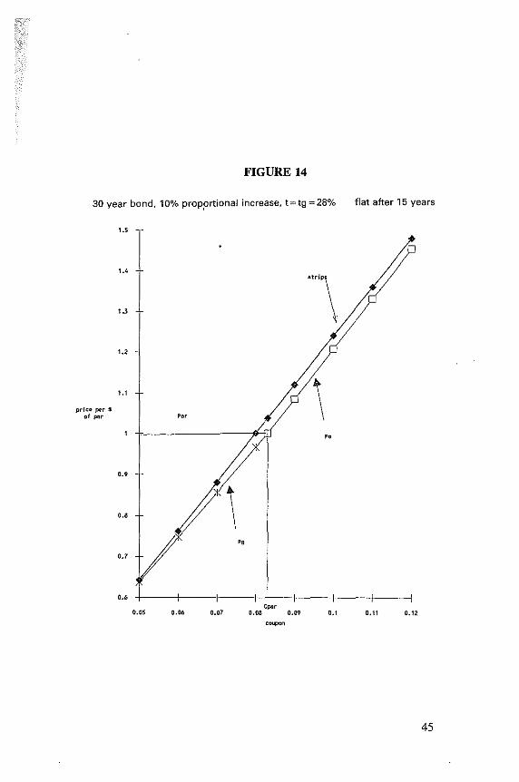
FIGURE 14

30 year bond, 10°/o propprtional increase, t=tg =28°/o flat after 15 years

1.S

1.4

1.3 '"'\ 1.2

1.1 \ prl~o:> per $ of par '"

"

0.9

0.8 \ .,

0.7

0.4

o.ns 0.06 0.07 '"" 0.08 0 . ., 0.1 0.11 0.12

'""""'

45

FIGURE 15

30 year bond, 5°/o proportional increase, t=tg=28o/o

price per s of par

46

1.5

, .3

'·'

0.9

0.1

o.5

0.03

"'

0.04 o.os '""' 0.06 0.07

per value of bond 6°/o

0.08 o." 0.,

FIGURE 16

30 year bond, 5o/o prop,ortional increase, t=tg=28°/o

price per S of pnr

1.5

1.3

.. ,

1.1

0.8

0.7

o.o

r

0.07 0.08 0.09 0.11 0.1Z

par value 10°/o

"

0.13 0.14

47

FIGURE 17

30 year bond, 5°/o proportional increase, t = tg = 28o/o par value of bond

price per $ of par

48

\.3

\.2

\.\

O.•

0.8

o.7

0.09

'"

\ "

0. \ o. 11 '"' 0.12 0, ll

strips

\

0.14

,,

0.15 o. 16

12°/o

FIGURE 18

30 year bond, 5o/o proportional increase, t = tg = 28o/o

,_,

1.2

'"

'·'

0.8

0.12 0.13

7 0.14 '"' 0, 15 (l.16

par value of bond 15°/o

strips

\ \

"

0.17 0.18 0.19

49

VII. Classification of Stripped Securities

The preceding results imply that (I) stripping will occur for rising yield curves, (2) long maturity bonds will be most profitable to strip, and (3) low coupon bonds will not be attractive to strip.

Term structures have been rising since September 1982 and stripping has occurred throughout the period. Table 11 classifies stripped securities by maturity and coupon level. This table is based upon CA TS, TIGRS, and STRIPS through July 1987.

The earlier examples showed that stripping is most profitable for coupon levels in an interval around par. This is essentially what Table 11 shows. Looking across the columns of Table 11, stripping is concen­trated among 16-20 yearand 26-30 year bonds. These are the newly issued 20 and 30 year bonds, which sell at par or close to par. Comparing the rows in the table, stripping is concentrated among coupon levels of 10% - 13%, placing the bonds stripped close to par. About 75% of the stripped bonds have maturities of 16 - 30 years and coupons of 10% - 13%.

Table 11. Classification of Stripped Securities by Coupon and Maturity as of July 1987-CATS, TIGRS, STRIPS.

Maturity (Years) Coupon Level

(%) 0-5 6-IO 11-15 16-20 21-25 26-30 Totals

7.00 - 7.99 8.00 - 8.99 0.07% 0.07% 9.00 - 9.99 2.21% 3.04% 5.25%

I0.00 - I0.99 1.06% 1.77% 10.86% 13.69% l l.00 - I l.99 11.15% 20.08%' 28.12% 59.35% 12.00 - 12.99 0.39% 5.48% 0.65% 2.94% 9.46% 13.00 - 13.99 0.95% 0.66% 1.01% 2.91% 2.22% 7.75% 14.00 - 14.99 1.56% 0.58% 2.09% 4.23% 15.00 - 15.99 0.44o/o 0.44%

Totals 2.51 o/o 15.54% l .02o/o 28.34% 5.65% 47.18% I00.24%'

*Total does not equal I OOo/o because of rounding errors.

50

VIII. Rebundling

In 1987, the Treasury began to allow the rebundling of STRIPS into underlying bonds. According to Treasury rules, a bond that was previously stripped, may be rebundled or reconstituted. Under Treasury rules, the par value of a particular bond must be used to rebundle that bond; coupons can be used interchangeably for rebundling. The Treasury restricts rebundling to existing underlying bonds. For example, if there are two 20-year bonds with 8% and 10% coupons in existence, only these two 20-year bonds can be created; a 12% coupon is not allowed under Treasury rules.

Table 12 shows the amount of STRIPS and the amount rebundled from May 1985 through August 1988. About 21 % of Treasury bonds are held in stripped form as of August 1988. The cumulative amount rebundled is 3.9%, implying a gross percent stripped of24.9% (i.e., 21 = 24.9 - 3.9, net stripping= gross stripping - rebundling).

If re bundling is permitted, bonds may be stripped at one point in time under one term structure. Later on, the bond may be rebundled because of a change in the term structure. There are a number of possible explanations of this. First, a bond may be stripped for a rising term structure. If the term structure becomes declining, rebundling may be profitable. Since term structure have been rising during 1987 and 1988, this cannot explain recent rebundling.

Second, shifts in the level of interest rates per se may cause rebundling. For example, it may be profitable to strip a par bond with a given rising term structure. If the level of yields changes, the original underlying par bond may have a higher value than a portfolio of strips. Rebundling the portfolio of strips may be profitable.

Tables 13 and 14 present an example in which a shift in the slope of the term structure makes rebundling desirable. Start with Table 13. This is an example of 30-year bonds with a rising term structure and a 28% tax rate. For each coupon level, the tax treatment with the highest value is marked with an asterisk. For bonds with coupons of7% and less, underlying bonds taxed by the regular income tax method have a greater value than strips. For coupons of So/o through 10%, strips have a greater value. Note that a par bond has a coupon of9.21 %. Therefore, the !0% coupon is a premium bond, which we assume to be taxed by linear amortization. We will focus on this !0% coupon bond, which is worth

51

Table 12. STRIPS

Cumulative Par Value of % of o/o of $Amount Underlying Par Amount Par Value Recon-

Bonds Value Stripped Recon- stituted Date ($Million) Stripped ($Million) stituted ($Million)

1985 May 31 $ 47,696 16.47% $ 7,855 June 30 47,696 19.96 9,520 July31 47,696 23.25 11,089 August 31 62,802 19.88 12,485 September 30 62,802 21.80 13,691 October 30 62,802 26.96 16,931 November 30 74,371 27.18 20,214 December 31 81,279 28.24 22,953

1986 January 31 81,281 29.79 24,214 February 28 105,391 24.62 25,947 March 31 105,392 25.23 26,590 April 30 105,392 25.34 26,706 May 31 124,864 21.69 27,083 June 30 124,874 22.19 27,710 July31 124,906 23.19 28,966 August 31 149,828 19.85 29,741 September 30 149,953 20.51 30,755 October 31 149,856 21.12 31,650 November 30 169,326 18.79 31,816 December31 169,329 19.16 32,443

1987 January 31 169,329 19.61 33,205 February 28 188,991 17.71 33,470 March 31 188,995 17.83 33,698 April 30 188,995 18.70 35,342 May31 208,280 17.46 36,186 June31 208,280 17.24 34,907 July 31 208,280 17.26 35,949 1.21% $ 2,520 August 31 226,728 15.96 36,186 1.27 2,879 September 30 226,728 17.23 39,065 1.78 4,036 October 31 226,728 19.00 43,078 2.05 4,648 November 30 241,477 19.13 46,195 2.62 6,327 December 31 241,477 18.54 44,770 2.77 6,689

1988 January 31 241,478 19.22 46,412 2.91 7,027 February 29 259,478 18.59 48,237 3.12 8,096 March 31 259,478 19.10 49,560 3.33 8,641 April 30 259,478 19.56 50,754 3.61 9,367 May31 277,352 18.98 52,631 3.44 9,546 June 30 277,352 19.56 54,239 3.63 10,057 July 31 277,352 20.20 56,031 3.79 10,511 August 31 287,947 21.09 60,722 3.86 11, 116

Source: Monthly Staremenr of Public Debt.

52

more as strips in Table 13. For coupons of 11% and higher, underlying bonds have greater value than strips.

Now, assume a drop in long-term interest rates resulting from a flatter term structure as shown in Table 14. See assumptions at bottom of the two tables. Focus on the 10% coupon bond. This bond has greater value as an underlying bond, whereas with the higher interest rate in Table 13 it was worth more as strips. Consequently, it will pay to rebundle strips into an underlying 10% coupon bond.

This example assumes a shift in the yield of30-year par bonds of about 1/2%, a change that can easily occur based upon recent history.

Table 13. Values of Bonds with 30.0 Period Maturities

Prices of Bonds for Different Tax Treatments

Regular Constant Linear Coupon Tax Yield Amortization STRIPS

.00000 0.1016 0.0627 0.0160 0.0627

.01000 0.1991* 0.1639 0.1228 0.1651

.02000 0.2967* 0.2655 0.2297 0.2676

.03000 0.3942* 0.3673 0.3365 0.3700

.04000 0.4918* 0.4691 0.4434 0.4725

.05000 0.5893* 0.5710 0.5502 0.5749

.06000 0.6869* 0.6728 0.6570 0.6774

.07000 0.7844* 0.7747 0.7639 0.7799

.08000 0.8820 0.8767 0.8707 0.8823*

.09000 0.9795 0.9786 0.9776 0.9848*

.09210 1.0000 1.0000 1.0000 1.0063*

.10000 1.0771 1.0805 1.0844 1.0872*

.11000 1.1746 1.1825 1.1913* 1.1897

.12000 1.2722 1.2844 1.2981* 1.2922

.13000 1.3697 1.3864 1.4049* 1.3946

.14000 1.4673 1.4884 1.5118* 1.4971

.15000 1.5648 1.5903 1.6186* 1.5995

.16000 1.6624 1.6923 1.7255* 1.7020

.17000 1.7599 1.7942 1.8323* 1.8044

.18000 1.8575 1.8962 1.9392* 1.9069

Assumptions: Number of Periods= 30 Tax Rate= 28o/o. Capital Gains Rate = 28% Forward rates increase geometrically by 3o/o. Forward rates are flat for maturity 10.0 years and longer. One Period Tax-Free Spot Rate is 0.0550.

*Indicates highest price for a given coupon level.

53

It is quite easy to construct other examples showing that even smaller shifts in the yield curve can create incentives to repackage securities.

The next section shows that in equilibrium the market values of STRIPS and underlying bonds must be equal. If there is a temporary disparity, arbitragers will enter the marketand strip or rebundle. It appears that the observed rebundling is part of the arbitrage process. To take advantage of temporary disparities, arbitragers repackage temporarily underpriced STRIPS into underlying bonds, driving prices towards equi­librium.

Table 14. Values of Bonds with 30.0 Period Maturities

Prices of Bonds for Different Tax Treatments

Regular Constant Linear Coupon Tax Yield Amortization STRIPS

.00000 0.1174 0.0766 0.0340 0.0766

.0!000 0.2193* 0.1829 0.1455 0. 1836

.02000 0.321 l * 0.2894 0.2570 0.2906

.03000 0.4230* 0.3959 0.3684 0.3976

.04000 0.5248* 0.5025 0.4799 0.5046

.05000 0.6267* 0.6091 0.5914 0.6116

.06000 0.7285* 0.7157 0.7028 0.7186

.07000 0.8304* 0.8223 0.8143 0.8256

.08000 0.9322 0.9290 0.9258 0.9325*

.08666 1.0000 1.0000 1.0000 1.0038*

.09000 1.0340 1.0356 1.0373 1.0395*

.!0000 1.1359 1.1423 1.1487* 1.1465

.1 !000 1.2377 1.2490 1.2602* 1.2535

.12000 1.3396 1.3556 1.3717* 1.3605

.13000 1.4414 1.4623 1.4831 * 1.4675

.14000 1.5433 1.5690 1,5946* 1.5745

. 15000 1.6451 1.6757 1.7061 * 1.6815

.16000 1.7469 1.7823 1.8175* 1.7884

.17000 1.8488 1.8890 1.9290* 1.8954

.18000 1.9506 1.9957 2.0405* 2.0024

Assumptions: Number of Periods= 30 Tax Rate= 28o/o. Capital Gains Rate= 28% Forward rates increase geometrically by 2%. Forward rates are flat for maturity 10.0 years and longer. One Period Tax·Free Spot Rate is 0.0550.

*Indicates highest price for a given coupon level.

54

IX. Stripping and the Pricing of Underlying Bonds

The introduction of stripping has had an impact upon the pricing of underlying bonds. To examine the relationship between the value of strips and underlying bonds, we will consider two cases: (I) The underlying bond can be stripped but strips cannot be rebundled. This corresponds to the actual situation for Treasury STRIPS from May I 985 to June 1987. (2) Underlying bonds can be stripped and strips can be rebundled. There may be repeated strippings and rebundlings. This corresponds to Treasury STRIPS beginning July 1987.

Case 1: The underlying bond can be stripped but strips cannot be rebundled. This is a case of an exchange option (see Margrabe (1978)) which can be exercised only once. In this case, the value of a strippable bond must be greaterthan the value of an otherwise identical nonstrippable bond or a portfolio of nonrebundlable strips, whichever is greater. Notation

P = market value of an underlying bond which cannot be stripped.

V = market value of strips which cannot be rebundled. PI = market value of an underlying bond which can be

stripped. Ifp;o, V, that is, ifa nonstrippable underlying bond has a value

greater than or equal to strips, a strippable bond must have a value at least as large as a nonstrippable bond because the strippable bond entitles the owner to the same cash flows as a nonstrippable bond, and it contains the option to strip, a non-negative addition to value. If P<V, that is, if the non­strippable underlying bond has a value lower than the strips, purchasing the bond for Pl and stripping would be profitable unless Pl ;o, V, i.e., the strippable bond has a value equaling or exceeding the value of strips.

Case 2: Underlying bonds can be stripped and strips can be rebundled. This case involves exchange options that can be exercised repeatedly. This is, the underlying bond can be stripped, the strips can be rebundled, the underlying stripped, etc. Notation

P2 = market value of a strippable bond. V2 = market value of portfolio of rebundlable strips.

55

Proposition: The market value of a strippable bond must equal the market value of the rebundlable strips, i.e., P2 = V2.

If this condition does not hold, there are arbitrage opportuni­ties. lfV2 > P2, then investors are able to buy bonds for P2, strip them, and sell the strips for V2 for a profit ofV2 - P2. This arbitrage makes the prices converge. If V2 < P2, then investors are able to buy strips, rebundle, and sell the underlying bond for a profit of P2 - V2. This arbitrage make the prices converge.

The price, P2, of a strippable bond is greater or equal to the higherof the value, P, of a nonstrippable underlying bond orthe value, V, of a nonrebundlable portfolio of strips. The price of the strippable bond exceeds these by the value of the options to exchange bonds for strips and vice versa.

Table 12 in the previous section showed the incidence of stripping and rebundling of STRIPS. If the market is always in equilib­rium, there is no advantage to strip or rebundle. But if the market is temporarily out of equilibrium (meaning underlying bonds are mispriced relative to strips or vice versa), stripping and rebundling are part of the ar­bitrage operations bringing market prices into line.

The result that P2 = V2 (i.e., the market value of strippable bonds equals the market value of rebundlable strips) has an interesting im­plication for the market segmentation argument. According to the seg­mentation view, there is special demand for strips by a subset of investors who desire to purchase zero coupon bonds. to 1neet their particular investment needs. This special demand is supposed to increase the prices and reduce the interest rates on strips relative to other bonds. This relative mispricing is impossible if P2 = V2. Arbitrage between strips and bonds keeps prices in line. Markets cannot be segmented if there is both stripping and rebundling. Conceivably, strong demand for a particular maturity of strip combined with arbitrage between markets might affect the shape of the yield curve. For example, strong demand for 30-year strips might push their interest rates lower; then, arbitrage b~tween markets will affect the rates on 30-year underlying bonds as well.

Propositio11: The price of a bond which can be stripped into rebundlable strips is at least as great as the price of a bond which can be stripped into nonrebundlable strips, i.e., P2 2' Pl.

Pl involves an option to strip, but not rebundle, whereas P2 involves an option to strip and rebundle repeatedly. P2 contains all the value of Pl plus something more, implying P2 has a higher value.

This proposition means that the Treasury has increased the market value of underlying bonds or reduced coupons on par bonds by

56

introducing rebundling in July 1987. In other words, the Treasury is better off to issue strippable bonds with rebundlable strips than to issue strips themselves.

The earlier discussion showed that strips may have a higher value than underlying bonds because of differences in the present values of tax payments. Before the Treasury STRIPS program, the Treasury effectively lost this incremental value. With rebundlable STRIPS, the Treasury captures this loss because it is able to sell bonds for the higher value of STRIPS.

57

X. Coupon Effects

A considerable literature has examined the relationship be­tween bond coupon level and yield to maturity (see Caks (1977), Living­ston (March 1979, September 1979, 1982)). For coupon-bearing bonds, taxation tends to create a positive coupon effect for discount bonds and a negative coupon effect for premium bonds. This section compares these results with the yields on strips. For rising term structures, strips have high yields, analogous to a negative coupon effect for premium bonds. This result has the important implication that high yields on strips do not necessarily indicate especially attractive investments but are the result of taxation.

The yield to maturity on a strip is the rate y satisfying the following equation:

F (l + y)" = FD(n) - ty (10.1)

In general, the yield to maturity is a complicated function of the term structure (i.e., D(j)) and the tax rate (t). The Appendix proves that the yield to maturity on a strip equals the yield to maturity on a par bond in the special case where the term structure is flat. Then, the yield to maturity on a strip equals R/(l - t), where R is the after-tax discount rate for every maturity.

By numerical analysis, we have found that the yield to maturity on a strip is greater (less) than the yield on a par bond for mono­tonically rising (falling) term structures. Since yield curves have been rising since 1982, we would expect that yields on strips have exceeded par bonds of the same maturity. This is illustrated

0

by the example in Table 15. Table 15 shows various yields to maturity for a rising term

structure with a regular income tax rate of28%. First, compare the yield to maturity on a par bond with those on strips. Strips have higher yields than par bonds for every maturity. Since strips are zero coupon bonds for the constant yield method, the coupon effect is negative for the constant yield method (i.e., lower coupon has higher yield to maturity). Note that the yield on a coupon-bearing discount bond taxed by the constant yield method would be between the yield on a strip and the yield on a par bond. This coupon effect is larger for long maturities, implying a steeper yield curve for strips than par bonds. This is, the par bond yield curve rises from

58

4.86% for one-year bonds to 7.18% for 29-year bonds. The strips yield curve rises from 4.86% for one-year bonds to 7 .72% for 29-year bonds.

Second, the yield on zero coupon bonds taxed by linear amortization has even a higher yield than strips, implying similar, but more extreme results.

Third, consider the yield on zero coupon bonds taxed by the capital gains (i.e., tg ; .4t) or regular income tax methods. For each of these, the yield on a zero coupon bond is less than the yield for par bonds, implying a positive coupon effect (i.e., lower coupon has lower yield to maturity). Thus, the sign of the coupon effect is positive for the capital gains and regular income tax methods, and negative for the constant yield method.

These results imply that care is required in interpreting the yield to maturity. Higher yields to maturity for strips may be the result of strips being fairly priced for a rising term structure. Higher yields per se do not indicate an especially attractive investment (See Caks (1977), Livingston (March 1979, September 1979)). The case of strips is another example where yield to maturity can be a misleading number. Higher yield does not mean greater investment value.

Table 15. Yields on Zeros versus Par Bonds.

Zero Coupon Yields

Capital Regular Tax-Free Tax-Free Gains Income Linear

N Forward Spot Par Tax Tax Strip Amortization

1.0 0.0350 0.0350 0.0486 0.0394 0.0486 0.0486 0.0486 3.0 0.0393 0.0371 0.0515 0.0416 0.0509 0.0516 0.0516 5.0 0.0442 0.0395 0.0546 0.0440 0.0533 0.0549 0.0550 7.0 0.0496 0.0420 0.0577 0.0466 0.0559 0.0585 0.0587 9.0 0.0558 0.0447 0.0610 0.0493 0.0586 0.0624 0.0629

11.0 0.0591 0.0473 0.0640 0.0520 0.0611 0.0663 0.0672 13.0 0.0591 0.0491 0.0661 0.0537 0.0626 0.0690 0.0704 15.0 0.0591 0.0504 0.0676 0.0549 0.0634 0.0710 0.0730 17.0 0.0591 0.0514 0.0687 0.0558 0.0640 0.0725 0.0754 19.0 0.0591 0.0523 0.0695 0.0564 0.0643 0.0737 0.0777 21.0 0.0591 0.0529 0.0702 0.0569 0.0644 0.0747 0.0799 23.0 0.0591 0.0534 0.0707 0.0573 0.0645 0.0755 0.0823 25.0 0.0591 0.0539 0.0712 0.0576 0.0645 0.0762 0.0850 27.0 0.0591 0.0543 0.0715 0.0579 0.0644 0.0767 0.0880 29.0 0.0591 0.0546 0.0718 0.0581 0.0644 0.0772 0.0916

Assumptions: Tax Rate= 2&o/o Forward rates increase geometrically by 6o/o. Forward rates are flat for maturity I 0.0 years and longer.

59

XI. Conclusion

Beginning in September 1982, several financial institutions began stripping U.S. Treasury securities, that is, decomposing the individ­ual coupons and par value and selling separate claims on each of the individual parts. This monograph shows that the July 1982 change in the tax law for original issue discount securities made it profitable for underwriters to strip U.S. Treasury securities for some term structures. In perfect markets with a rising term structure, a decomposition of an under­lying bond into a portfolio of individual strips created a higher value. The resulting profit opportunities have contributed to underwriter incentives to strip U.S. Treasury securities.

In May 1985, the U.S. Treasury began to allow stripping of U.S. Treasury securities by book entry. This low-cost method of stripping, called STRIPS, has come to dominate the market. In July 1987, the Treasury permitted STRIPS to be rebundled into underlying bonds. Changes in the level of interest rates cause stripping or rebundling. The options to strip and re bundle have affected the pricing ofunderlying bonds, whose prices must include the value of these stripping and rebundling options.

60

Appendix A

Proposition. For a flat term structure in which R(l) = R(2) = ... = R(n) = R, the yield to maturity (y) for bonds taxed by the yield method (including strips) is equal to R/(l - t) Proof

Py = c(l - t) A(n) + FD(n)

D(j) - t[y(c, n)F - c] L (I + y(c n))"-i"

J"'l ,

(A.I)

If y = R/(l - t) then

Py= (c(l - t)/R) [I - (I+ R)-"] + F(l + R)""

- [t(yF - c)/(y - R)] [(I + R)-" - (I + y)""] (A.2)

This simplifies to

Py= (c/y) [I - (I + y)""] + F(l + y)-" (A.3)

which is the price expressed in terms of yield to maturity. Only if y =RI (I - t) is the condition in (A-3) satisfied.

Proposition. If V is the market value of individual strips defined in equation (7), V = Py for a flat term structure. Proof

[ "." D(j)

V - Py= ct A(n) - I y(O, J) I (I (O '))i-'" J=I 1=l +y ,J

" D(j) J [ " D(j) -ti (I +y(c, n))"-i'' + tF y(c, n) ~' (I +y(c, n))"·i•t

" D(j) J - y(O, n) ti (I +y(O, n))"-i" (A.4)

61

For a flat term structure y(c, n) = y (0,j) for all c and allj. Consequently, the second bracketed term equals zero. Substituting for the summation in the first bracketed term results in ct times

" R·' [I - (l+R)-"] - (y/(y-R)) 2: [(l+r)-i. (l+y)·i] j=l

- (l/(y-R))[(l-R)·" - (l+y)·"]

Take the sum in the second term

-[-1-J[(l+R)'" - (l+y)'"] y-R

The (I - y)'" terms cancel. Combining terms result in

[ 1-(l+R)'"][l-2'__]-[-l J[l -(l+R)'"] R y-R y-R

[ 1 - (l+R)·"] [ _R_ ]~[-I J [I - (l+R)'"]

R y-R - , y-R

This nets to zero.

62

(A.5)

(A.6)

(A.7)

(A.8)

Appendix B

According to the tax law, the basis for a bond taxed by the constant yield method with original yeild to maturity of y and periodic coupon c is determined by HU+!, n) =HU, n) (l+y) - c. The basis for individual points in time will be

Point in time Basis

0 Py Py(l + y) - c

2 Py(l + y)2 - c(l + y) - c 3 Py(! + y)3 - c(l + y)2 - c(l + y) - c

j Py(! + y)i- c(l + y)H - c(l +y)i·2 - ••• c(l + y) - c

The basis for point in time j can be rewritten as

H . . y·[ c c c J U,n)=(l+y)'Py-(I+y I+y + (l+yJ2+ ... +(l+y)i (B.l)

Since Py= I c(l+y)·k + F(l+y)·", k

" = I c(l +y)·»i + F(l +y)·"'i k=j+l

n-j

= I c(I +y)·k + F(l +y)·"'i k=I

(B.2)

(B.3)

(B.4)

(B.5)

63

Appendix C

Derivation of Conditions in Table 7

Discou11t Bo11ds Since Pa-< Py-< Pr< Pg-, ifV -Py= 0, Pa-< V <Pr <Pg­ifV -Py< 0, V <Py-<Pr<Pg­if V - Py > 0, V > Py-

ParB011ds Since Pa0 = Py0 = Pt0 = Pg0,

if V - Py = 0, V = Pa0 = Py0 = Pt0 = Pg0

ifV -Py< 0, V <all if V - Py> 0, V >all

Pre1niu1n Bonds Since Pa+ >Py+ > Pt+> Pg+, ifV -Py= 0, Pa+> V >Pt+> Pg+ ifV -Py< 0, Pa+ >Py+> V ifV -Py >0, V >Py+ >Pt' >Pg+

64

(C.l) (C-2) (C.3) (C.4)

(C.5) (C.6) (C.7) (C.8)

(C.9) (C. 10) (C.11) (C.12)

References

Ang, James, David Peterson and Pamela Peterson. "Marginal Tax Rates: Evidence from Nontaxable Corporate Bonds: A Note," Journal of Finance (March 1985), pp. 327-332.

Arditti, Fred and Miles Livingston. "The Relative Price Volatility of Taxable and Non-Taxable Bonds: A Note," Journal of Finance (June 1982), pp. 877-881.

Becketti, Sean. "The Role of Stripped Securities in Portfolio Management," Econon1ic Revieiv Federal Reserve Bank of St. Louis73 (May 1988), pp. 20-3 I.

Bierwag, Gerald 0. "Immunization, Duration and the Term Structure of Interest Rates," Journal of Financial and Quantitative Analysis (December 1977), pp. 725-742.

Bench, Joseph. "Zero Coupons vs. Conventional Bonds," Banker's Monthly Magazine (September 15, 1984).

Boquist, John. "Coupon Stripping, Arbitrage and Market Equilibrium," paper pre­sented at Eastern Finance Association Meetings, April 11 - 14, 1984.

Brooks, Robert, Haim Levy and Miles Livingston. "The Coupon Effect on Term Premiums," Journal of Financial Research (forthcoming).

Caks, John. "The Coupon Effect on Yield Maturity," Journal of Finance 32 (1977), pp. 103-115.

Chakravarty, Subrata N. "Things Won't Go Better with Pepsi,'' Forbes (May 24, 1982), p. 177.

"In Breeding," The Banker (September 1982), p. 91. "A Rediscovered Wheel,'' The Banker (January 1987), p. 43. Constantinides, George M. and Jonathan E. Ingersoll. "Optimal Bond Trading

with Personal Taxes," Journal of Financial Eco1101nics 13 (September 1984), pp. 299-335.

Dun's Business Month (July 1984). "The Compelling Case for T-Bond Zeros." Fisher, Lawrence and Roman L. Weil. "Coping with the Risk of Interest Rate Fluc­

tuations: Returns to Bondholders from Naive and Optimal Strategies," Journal of Business (October 1971 ), pp. 408-431.

Hopewell, Michael and George G. I(aufman. "Bond Price Volatility and Years to Maturity," An1erica11 Eco110111ic RevieH' (September 1973), pp. 749-759.

Internal Revenue Service. list of Original Issue Discount Obligations. U.S. Gov­ernment Printing Office, Department of the Treasury (November 1984).

Kanemasu, Hiromitsu, Robert H. Litzenberger, and Jacques Rolfo. "Financial Innovation in an Incomplete Market: An E1npirical Study of Stripped Government Securities," unpublished working paper (September 1986).

Kaufman, GeorgeG. "The Case for the Long-Tern1 Zero-Coupon Treasury Bonj," Banker's Magazine (Autumn 1973), pp. 35-39.

65

Kluber, Thomas and Thomas Stauffacher. "Zero Coupon Treasury Securities," in Handbook of Treasury Securities: Trading and Portfolio Strategies, edited by Frank J. Fabozzi. Probus Publishing (1987).

"Legal Tempest over TIGRs," Investment Dealer's Digest (February 19, 1985). Litzenberger, Robert and Jacques Rolfo. "An International Study of Tax Effects

of Government Bonds," Journal of Finance (March 1984), pp. 1-22. Litzenberger, Robert and Jacques Rolfo. "Arbitrage Pricing, Transaction Costs

and Taxation of Capital Gains: A Study of Government Bonds with the Same Maturity Date," Journal of Financial Econon1ics 13 (September 1984), pp. 337-351.

Livingston, Miles. ''Taxation and Bond Market Equilibrium in a World of Uncertain Future Interest Rates," Journal of Financial and Quantitative Analysis 14 (March 1979), pp. 11-27.

Livingston, Miles. "Bond Taxation and the Shape of the Yield to Maturity Curve," Journal of Finance 34 (March 1979), pp. 189-196.

Livingston, Miles. "A Note on the Issuance of Long-Tenn Pure Discount Notes," Journal of Finance 34 (March 1979), pp. 179-193.

Livingston, Miles. "The Pricing of Premium Bonds," Journal of Financial and Quantitative Analysis 14 (September 1979), pp. 517-527.

Livingston, Miles. "The Pricing of Municipal Bonds," Journal of Financial and Quantitative Analysis 17 (June 1982), pp. 179-193.

Mamis, Robert A. "A Deal for All Seasons," Inc. (January 1986), pp. 105-110). Margrabe, William. "The Value of an Option to Exchange One Asset for Another,"

Journal of Finance 33 (1978), pp. 177-186. Merrill Lynch, Inc. "TIGR Cubs: Safe Enough for the Tamest Investor,"

Investments for a Changing Econon1y (Spring 1984). "Merrill Lynch Is Sued Over Pricing of 'Tigers'," New York Tin1es (February I,

1985). Miller, Merton H. "Debt and Taxes," Journal of Finance 32 (1977), pp. 261-275. Monthly Staten1ent of the Public Debt. U.S. Government Printing Office. Nagan, Peter S. and Kenneth A. Kaufman. "STRIPS-An Exciting New Market

for Zero-Coupons," ABA Banking Journal (March 1985), pp. 12-13. Panich, Richard L. and S.E.C. Previs. "Amortization of Premium, Acquisition

Premium and Market Discount," The Tax Auditor (January 1988), pp. 54-63. •

Panich, Richard L. and S.E.C. Previs. "Amortization of Discount on OID Bonds and Short-Tenn Obligations," The Tax Advisor (November 1987), pp. 840-849.

Petre, Peter D. "Why Zero-Coupon Securities Are Hot," Fortune (October 18, 1982).

Pyle, David. "Is Deep Discount Debt Financing a Bargain?" Chase Financial Quarterly (Fall 1981).

Redington, F. M. "Review of the Principle of Life Office Valuations," Journal of the Institute of Actuaries 18 (1952), pp. 286-340.

Robichek, A. and W. Niebuhr. "Tax Induced Bias in Reported Treasury Yields," Journal of Finance (December 1970), pp. 1081-1090.

66

Rosen, Lawrence R. Investing in Zero Coupon Bonds. New York: John Wiley and Sons (1986),

Salomon Brothers, Inc. Robert W. Kopprasch, "Callable CATS vs Similar Products-A Comparison of Yield Calculations" (June 1, 1983); Thomas E. Klaffkey and Frances Sirianni, "Cats Market Update-March 1984" (April 18, 1984); Robert W. Kopprasch and Daniel L Schwarz, "The Analysis of Serial CATS" (February 29, 1984); Thomas E. Klaffky, "The CATS Market at the Beginning of 1984" (January 1984); Thomas E. Klaffky, "The New World of Coupon Stripping" (August 1982); Thomas E. Klaffky and Robert W. Kopprasch, "Understanding the Volatility of CATS and Other Zero-Coupon Bonds" (May 1983); "Treasury Zero Update" (January 1986, April 1986, July 1986, January 1987, April 1987, July 1987).

Samuelson, P.A. "The Effect Of Interest Rate Increases on the Banking System," American Econon1ics Review (March 1945), pp. 16-27.

Schaefer, Stephen M. "Tax Induced Clientele Effects in the Market for British Government Securities," Journal of Financial Eco1101nics 10 (July 1982), pp, 121-159.

"Selecting Zero-Coupon Municipals," New York Times (February 3, 1985). "Setting Prices of Zero-Coupon Bonds," NeH' York Times (January 27, 1985). Skelton, J. L. "Relative Risk in Municipal and Corporate Debt," Journal of

Finance 38 (May 1983), pp. 625-634. "Stags at Bay," Banker (September 1985), pp. 106-107. Trczinka, C. "The Pricing of Tax-Exempt Bonds and the Miller Hypothesis,"

Journal of Finance 37 (September 1982), pp. 907-924. "U.S. is Altering Rules to Accommodate Growing Market in 'Zero-Coupon'

Bonds," Wall Street Journal (January 16, 1985). Van Horne,J. Financial Market Rates and Flows. Englewood Cliffs, New Jersey:

Prentice-Hall (1984). Weber, Ben. "Commander Zero," Forbes (September IO, 1984). Webenman, Ben. "Zero Coupon Bombs," Forbes (January 26, 1987), p. 103. Webennan, Ben. "Get Set for a Striptease," Forbes (January 18, 1982), p. 109. Woolridge, J. Randall and Gary Gray. "Are Original-Issue Discount Bonds Here

to Stay?" Harvard Business Review (May/June 1982), pp. 54-56. "Zero-Coupon Bonds' Price Savings Jolt Investors Looking for Security," Wall

Street Journal (June I, 1984). "Zero Plus Zero Equals ... ,' Barron's (September 24, 1984). "Zero Coupons Strike Again," Banker (November 1985), pp. 68-69.

67