Embed Size (px)
Citation preview
Procedia - Social and Behavioral Sciences 96 ( 2013 ) 933 – 944
1877-0428 © 2013 The Authors. Published by Elsevier Ltd. Open access under CC BY-NC-ND license.Selection and peer-review under responsibility of Chinese Overseas Transportation Association (COTA).doi: 10.1016/j.sbspro.2013.08.107
ScienceDirect
13th COTA International Conference of Transportation Professionals (CICTP 2013)
The strain field model and its modification of semi-rigid asphalt pavement with graded granular interlayer
Zhongyin Guoa,Shaohui Lia*,Yongshun Yangb
aSchool of Transportation Engineering,Tongji University,Shanghai 201804,ChinabHighway Bureau of Transportation Office,Shandong Provincb e,Jinan 250002,Chinae
Abstract
In order to model the strain distribution field of semi-rigid asphalt pavement with a graded gravel interlayer, both numericalsimulations and field tests are conducted. Through numerical simulations with different interface conditions and axles, inwhich the constitutive model is stress dependent, the strain model is obtained. At the same time, experiment road with a length of 200 meters is built in field in Shandong province and with the strain detectors buried in the road, strains underdifferent axle loads are also obtained. The simulated strain model was statistically tested for significance and factors havingsignificant influence on pavement strain are obtained.
© 2013 The Authors. Published by Elsevier B.V.Selection and/or peer-review under responsibility of Chinese Overseas Transportation Association (COTA).
Keyword:Graded gravel interlayer, strain detector, strain field distribution model,modification ,significant test
1. introduction
The most important factor affecting the modulus of granular is the stress condition it is bearing. Some of themodels only give a definition of the resilient modulus and Poisson s ratio, and these types of models are usuallybased on observation from RTL test results, such as the k-theta model(Seed et al. 1967b). This k-theta model is akind of resilient model and the resilient modulus is used as a surrogate elastic modulus in Hooke s Law do definethe stress-strain relationship. This kind of law can be called curve-fit model. The earliest non-linear model for cyclic loading of granular materials was proposed in 1962 by Biarez(1961) and it can be described as :
(1)The meaning of the values are:
* Corresponding author. Tel.: 021-69585413; fax: 021-69585413.E-mail address: [email protected]
Available online at www.sciencedirect.com
© 2013 The Authors. Published by Elsevier Ltd. Open access under CC BY-NC-ND license.Selection and peer-review under responsibility of Chinese Overseas Transportation Association (COTA).
934 Zhongyin Guo et al. / Procedia - Social and Behavioral Sciences 96 ( 2013 ) 933 – 944
E=secant modulus; K, n=empirical constants; =mean normal stress= Then after six years, this model was modified by Seed et al (1967b) and the new model replaced the secant
modulus with the resilient modulus and the mean normal stress with the first invariant of the stress tensor or bulk stress which can be described as :
(2) Where: Mr=resilient modulus; k1 ,n= constants; J1= = This model is known as the K- model, but the new model as it is proposed is not dimensionally correct. In
order to normalize the bulk stress, the unit stress or atmospheric pressure to allow it to be raised to a power. So the second model where the bulk stress was replaced by confining stress as this (1967a):
(3) A non-linear FEM study to determine the sensitivity of various input factors is undertaken by Allen and
Thompson(1974b). One of their conclusions was that if the n of the k-theta model is held at a constant value and the k1 varied, the percentage change in the pavement response such as the deflections on the pavement surface and the strains of the subgrade is much less than the percentage change in the parameter. A major shortage of the model is that the effect of shear stress is not taken into a consideration and that multiple stress conditions will make the same modulus predictions. For example: low values of confining( 2/ 3) stress and high axial stress 1 will have the same bulk stress value as a stress state where the confining stress is high and the axial stress is low. This situation makes the model not work as good as we expect.
Shackle (1973) proposed a three parameter model using two functions of the stress state as follows: (4)
Where: k1.k2,k3:constants; : octahedral normal stress : octahedral shear stress
A model of essentially the same form as equation(5) was proposed by Uzan (1985), but the octahedral normal stress was replaced by the bulk stress and the octahedral shear stress with the deviatoric stress. The Uzan-Witzcak has been defined with the shear stress term reverting to the octahedral shear stress, the change to the non-dimensional power terms and finally the addition of 1 to the shear stress term to remove the singularity that occurs when the shear stress term is equal to zero(Andrei et al ,2004). It can be described as follows:
(5) Where: pa: atmospheric pressure(100KPa) This model is referred to as Uzan model, as most researchers have attributed its origin to Uzan. The Dresden model , proposed by Wellner and Gleitz(1999), can be used to determine the modulus and
Poisson s ratio from RTL tests and it can be shown as: (6)
This model requires eight parameters and has the advantage of providing a nominal stiffness k5 when the stress level are low. However, this value cannot be determined from RTL tests as the definition of resilient modulus does not allow for a 0 stress result. The Dresden model is also not dimensionally correct in its published form.
Andrei et al(2004) examined a number of different log-log and semi-log formulations of two parameter models( ) and up to 5 constants and concluded that the best representation of Mr in terms of accuracy, implementation and numerical stability was equation(5).
In FEM, the entire load is applied in one step and the calculation is repeated until the moduli used in the solution are equal to or within a specified error of the moduli calculated from the stress extracted from the solution and in this method, its solution is usually formulated as a first order Cauchy or Hookean stress strain problem. Through review of the resilient model of the unbounded materials, the strain prediction model form abide by the theory will be obtained and by the field strain measured by strain detectors, modifications to the strain model will be available.
935 Zhongyin Guo et al. / Procedia - Social and Behavioral Sciences 96 ( 2013 ) 933 – 944
2. Experimental methodology
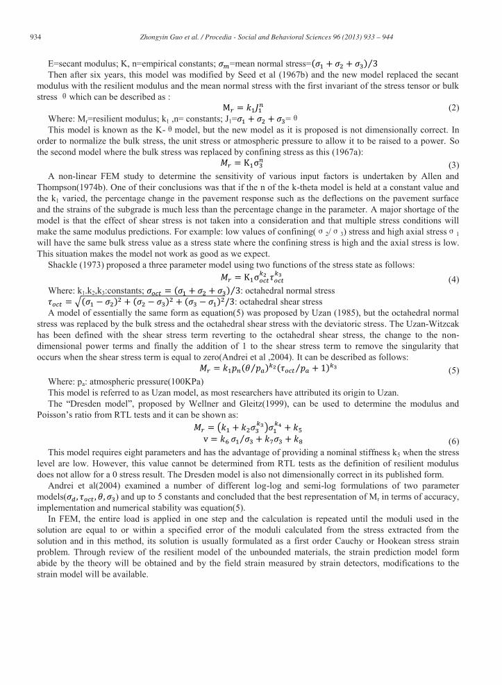
In order to investigate the strain field distribution at critical points, experiment road is constructed in ShanDong province and some strain detectors, by which the strains can be measured, have been buried in thepavement. The strain detectors are shown in figure 1.
Fig. 1 the I-beam strain detectorr
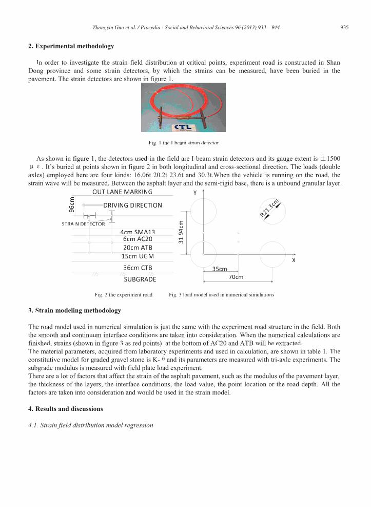
As shown in figure 1, the detectors used in the field are I-beam strain detectors and its gauge extent is 1500. It s buried at points shown in figure 2 in both longitudinal and cross-sectional direction. The loads (double
axles) employed here are four kinds: 16.06t 20.2t 23.6t and 30.3t.When the vehicle is running on the road, thestrain wave will be measured. Between the asphalt layer and the semi-rigid base, there is a unbound granular layer.
OUT LANE MARKING
DRIVING DIRECTION
96cm
STRAIN DETECTOR4cm SMA136cm AC2020cm ATB15cm UGM
36cm CTB
SUBGRADE
X
Y
RRR21.3cmmm
31.94cm
35cm70cm
Fig. 2 the experiment road Fig. 3 load model used in numerical simulations
3. Strain modeling methodology
The road model used in numerical simulation is just the same with the experiment road structure in the field. Both the smooth and continuum interface conditions are taken into consideration. When the numerical calculations arefinished, strains (shown in figure 3 as red points) at the bottom of AC20 and ATB will be extracted.The material parameters, acquired from laboratory experiments and used in calculation, are shown in table 1. Theconstitutive model for graded gravel stone is K- and its parameters are measured with tri-axle experiments. Thesubgrade modulus is measured with field plateff load experiment.There are a lot of factors that affect the strain of the asphalt pavement, such as the modulus of the pavement layer,the thickness of the layers, the interface conditions, the load value, the point location or the road depth. All thefactors are taken into consideration and would be used in the strain model.
4. Results and discussions
4.1. Strain field distribution model regression
936 Zhongyin Guo et al. / Procedia - Social and Behavioral Sciences 96 ( 2013 ) 933 – 944
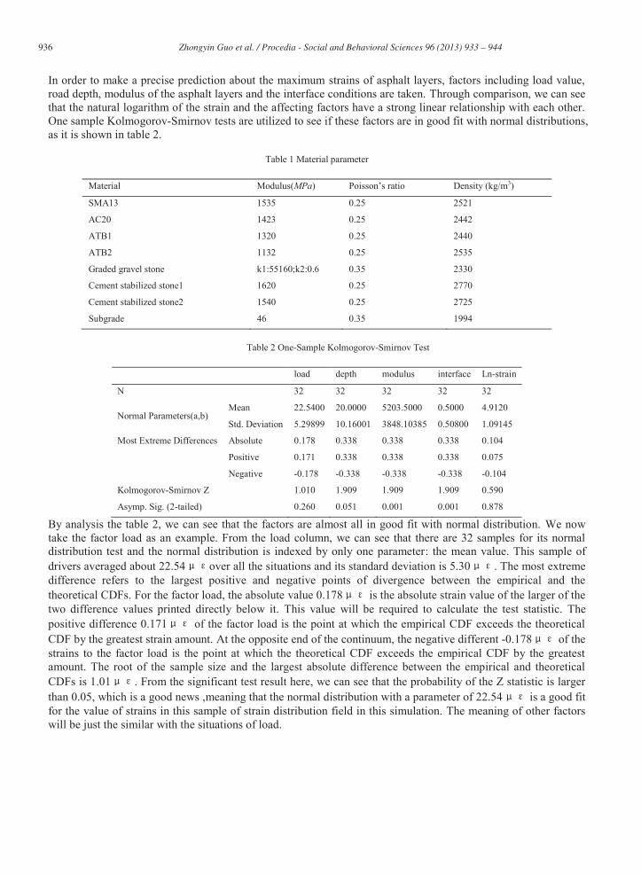
In order to make a precise prediction about the maximum strains of asphalt layers, factors including load value, road depth, modulus of the asphalt layers and the interface conditions are taken. Through comparison, we can see that the natural logarithm of the strain and the affecting factors have a strong linear relationship with each other. One sample Kolmogorov-Smirnov tests are utilized to see if these factors are in good fit with normal distributions, as it is shown in table 2.
Table 1 Material parameter
Material Modulus(MPa) Poisson s ratio Density (kg/m3)
SMA13 1535 0.25 2521
AC20 1423 0.25 2442
ATB1 1320 0.25 2440
ATB2 1132 0.25 2535
Graded gravel stone k1:55160;k2:0.6 0.35 2330
Cement stabilized stone1 1620 0.25 2770
Cement stabilized stone2 1540 0.25 2725
Subgrade 46 0.35 1994
Table 2 One-Sample Kolmogorov-Smirnov Test
load depth modulus interface Ln-strain
N 32 32 32 32 32
Normal Parameters(a,b) Mean 22.5400 20.0000 5203.5000 0.5000 4.9120
Std. Deviation 5.29899 10.16001 3848.10385 0.50800 1.09145
Most Extreme Differences Absolute 0.178 0.338 0.338 0.338 0.104
Positive 0.171 0.338 0.338 0.338 0.075
Negative -0.178 -0.338 -0.338 -0.338 -0.104
Kolmogorov-Smirnov Z 1.010 1.909 1.909 1.909 0.590
Asymp. Sig. (2-tailed) 0.260 0.051 0.001 0.001 0.878
By analysis the table 2, we can see that the factors are almost all in good fit with normal distribution. We now take the factor load as an example. From the load column, we can see that there are 32 samples for its normal distribution test and the normal distribution is indexed by only one parameter: the mean value. This sample of drivers averaged about 22.54 over all the situations and its standard deviation is 5.30 . The most extreme difference refers to the largest positive and negative points of divergence between the empirical and the theoretical CDFs. For the factor load, the absolute value 0.178 is the absolute strain value of the larger of the two difference values printed directly below it. This value will be required to calculate the test statistic. The positive difference 0.171 of the factor load is the point at which the empirical CDF exceeds the theoretical CDF by the greatest strain amount. At the opposite end of the continuum, the negative different -0.178 of the strains to the factor load is the point at which the theoretical CDF exceeds the empirical CDF by the greatest amount. The root of the sample size and the largest absolute difference between the empirical and theoretical CDFs is 1.01 . From the significant test result here, we can see that the probability of the Z statistic is larger than 0.05, which is a good news ,meaning that the normal distribution with a parameter of 22.54 is a good fit for the value of strains in this sample of strain distribution field in this simulation. The meaning of other factors will be just the similar with the situations of load.
937 Zhongyin Guo et al. / Procedia - Social and Behavioral Sciences 96 ( 2013 ) 933 – 944
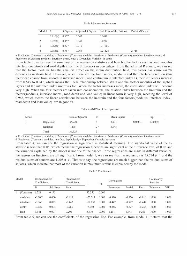
Table 3 Regression Summary
Model R R Square Adjusted R Square Std. Error of the Estimate Durbin-Watson
1 0.810(a) 0.657 0.645 0.64991
2 0.925(b) 0.857 0.847 0.42741
3 0.963(c) 0.927 0.919 0.31005
4 0.984(d) 0.967 0.963 0.21128 2.710
a Predictors: (Constant), modulus; b Predictors: (Constant), modulus, interface; c Predictors: (Constant), modulus, interface, depth; d Predictors: (Constant), modulus, interface, depth, load; e Dependent Variable: ln-strain From table 3, we can see the summary of the regression statistics and how big the factors such as load modulus interface conditions and road depth affect the differences in percentage. From the adjusted R square, we can see that the factor modulus has the smallest effect on the strain distribution field, this factor can cause 64.5% differences in strain field. However, when these are the two factors, modulus and the interface condition (this factor can change from smooth in interface index 0 and continuum in interface index 1), their influences increase from 0.645 to 0.847, which means the linear relationship between strain and the factors modulus of the asphalt layers and the interface index improves too. When the factor increases more, the correlation index will become very high. When the four factors are taken into considerations, the relation index between the ln-strain and the factors(modulus, interface index , road depth and load value) in linear form is very high, reaching the level of 0.963, which means the linear correlations between the ln-strain and the four factors(modulus, interface index , road depth and load value) are in good fit.
Table 4 ANOVA of the regression
Model Sum of Squares df Mean Square F Sig.
1 Regression 35.724 4 8.931 200.063 0.000(d)
Residual 1.205 27 0.045
Total 36.929 31
a Predictors: (Constant), modulus; b Predictors: (Constant), modulus, interface; c Predictors: (Constant), modulus, interface, depth d Predictors: (Constant), modulus, interface, depth, load; e Dependent Variable: ln-strain From table 4, we can see the regression is significant in statistical meaning. The significant value of the F-statistic is less than 0.05, which means the regression functions are significant at the difference level of 0.05 and the variation explained by the model is not due to the chance. If the regressions are made in different variables, the regression functions are all significant. From model 1, we can see that the regression is 35.724 and the residual sums of squares are 1.205 . That is to say, the regressions are much bigger than the residual sums of squares, which indicate that most of the variation in maximum strains is explained by the model.
Table 5 Coefficients
Model Unstandardized Coefficients
Standardized Coefficients t Sig.
Correlations Collinearity Statistics
B Std. Error Beta Zero-order Partial Part Tolerance VIF
1 (Constant) 6.228 0.193 32.350 0.000
modulus -0.0001 0.000 -0.810 -23.311 0.000 -0.810 -0.976 -0.810 1.000 1.000
interface -0.960 0.075 -0.447 -12.852 0.000 -0.447 -0.927 -0.447 1.000 1.000
depth -0.029 0.004 -0.266 -7.640 0.000 -0.266 -0.827 -0.266 1.000 1.000
load 0.041 0.007 0.201 5.770 0.000 0.201 0.743 0.201 1.000 1.000
From table 5, we can see the coefficients of the regression line. For example, from model 1, it states that the
938 Zhongyin Guo et al. / Procedia - Social and Behavioral Sciences 96 ( 2013 ) 933 – 944
expected ln-strain is equal to 0.041*load-0.029*depth-0.960*interface condition index-0.0001*modulus+6.228 or this function can be shown in formula 7.
(7) If a particular vehicle is running on the road surface, the maximum strain of the road can be calculated by formula 7. The sig values of F-test for model 4 are all 0, which means the independent variables (load, modulus, road depth, interface condition index) have significant effect on the maximum strains. The zero order correlations tests and the part correlations tests of the four factors are almost the same, which means the variations explained by the four independents and it cannot be explained by other independents. That is to say, the formula is unique. The tolerance values for the four factors are all 1.000 and VIFs are 1.000, which means the four factors have no col-linearity problems.
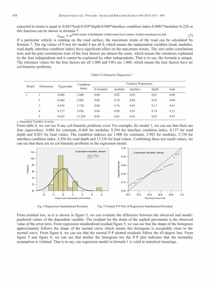
Table 6 Collinearity Diagnostics a
Model Dimension Eigenvalue Condition Index
Variance Proportions
(Constant) modulus interface depth load
1 1 4.086 1.000 0.00 0.02 0.02 0.01 0.00
2 0.460 2.982 0.00 0.10 0.88 0.01 0.00
3 0.294 3.730 0.00 0.76 0.05 0.17 0.01
4 0.137 5.456 0.04 0.09 0.03 0.74 0.12
5 0.023 13.258 0.96 0.03 0.02 0.07 0.87 a Dependent Variable: ln-strain From table 6, we can see if any col-linearity problems exist. For example, for model 1, we can see that there are four eigenvalues: 4.086 for constants, 0.460 for modulus, 0.294 for interface condition index, 0.137 for road depth and 0.023 for load values. The condition indexes are 1.000 for constants, 2.982 for modulus, 3.730 for interface condition index, 5.456 for road depth and 13.256 for load values. Combining these test result values, we can see that there are no col-linearity problems in the regression model.
Fig. 4 Regression Standardized Residual Fig. 5 Normal P-P Plot of Regression Standardized Residual
From residual test, as it is shown in figure 5, we can evaluate the difference between the observed and model-predicted values of the dependent variable. The residual for the strain of the asphalt pavements is the observed value of the error term. From regression standardized residual figure 5, we can see that the shape of the histogram approximately follows the shape of the normal curve which means this histogram is acceptably close to the normal curve. From figure 6, we can see that the normal P-P plotted residuals follow the 45-degree line. From figure 5 and figure 6, we can see that neither the histogram nor the P-P plot indicates that the normality assumption is violated. That is to say, our regression model in formula 1 is valid in statistical meanings.
939 Zhongyin Guo et al. / Procedia - Social and Behavioral Sciences 96 ( 2013 ) 933 – 944
4.2. Strain model modification
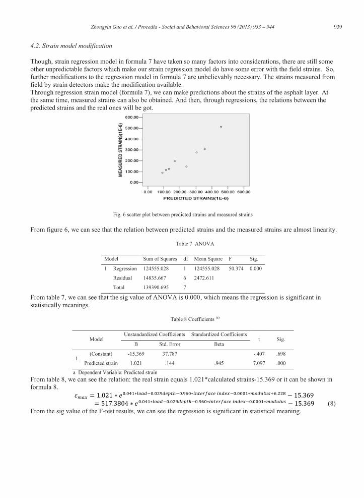
Though, strain regression model in formula 7 have taken so many factors into considerations, there are still some other unpredictable factors which make our strain regression model do have some error with the field strains. So, further modifications to the regression model in formula 7 are unbelievably necessary. The strains measured from field by strain detectors make the modification available. Through regression strain model (formula 7), we can make predictions about the strains of the asphalt layer. At the same time, measured strains can also be obtained. And then, through regressions, the relations between the predicted strains and the real ones will be got.
Fig. 6 scatter plot between predicted strains and measured strains
From figure 6, we can see that the relation between predicted strains and the measured strains are almost linearity.
Table 7 ANOVA
Model Sum of Squares df Mean Square F Sig.
1 Regression 124555.028 1 124555.028 50.374 0.000
Residual 14835.667 6 2472.611
Total 139390.695 7
From table 7, we can see that the sig value of ANOVA is 0.000, which means the regression is significant in statistically meanings.
Table 8 Coefficients (a)
Model Unstandardized Coefficients Standardized Coefficients
t Sig. B Std. Error Beta
1 (Constant) -15.369 37.787 -.407 .698
Predicted strain 1.021 .144 .945 7.097 .000
a Dependent Variable: Predicted strain From table 8, we can see the relation: the real strain equals 1.021*calculated strains-15.369 or it can be shown in formula 8.
(8)
From the sig value of the F-test results, we can see the regression is significant in statistical meaning.
940 Zhongyin Guo et al. / Procedia - Social and Behavioral Sciences 96 ( 2013 ) 933 – 944
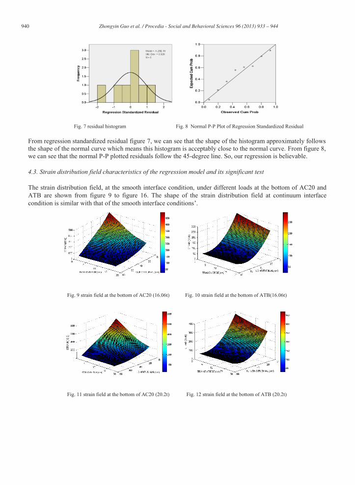
Fig. 7 residual histogram Fig. 8 Normal P-P Plot of Regression Standardized Residual
From regression standardized residual figure 7, we can see that the shape of the histogram approximately follows the shape of the normal curve which means this histogram is acceptably close to the normal curve. From figure 8, we can see that the normal P-P plotted residuals follow the 45-degree line. So, our regression is believable.
4.3. Strain distribution field characteristics of the regression model and its significant test
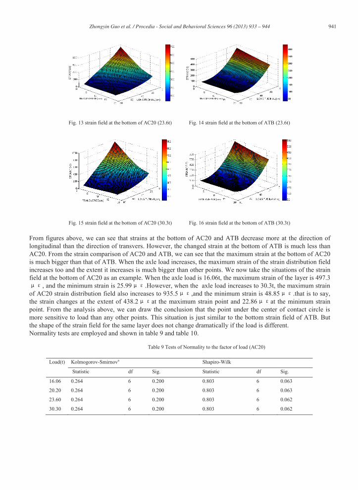
The strain distribution field, at the smooth interface condition, under different loads at the bottom of AC20 and ATB are shown from figure 9 to figure 16. The shape of the strain distribution field at continuum interface condition is similar with that of the smooth interface conditions .
Fig. 9 strain field at the bottom of AC20 (16.06t) Fig. 10 strain field at the bottom of ATB(16.06t)
Fig. 11 strain field at the bottom of AC20 (20.2t) Fig. 12 strain field at the bottom of ATB (20.2t)
941 Zhongyin Guo et al. / Procedia - Social and Behavioral Sciences 96 ( 2013 ) 933 – 944
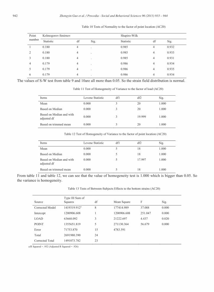
Fig. 13 strain field at the bottom of AC20 (23.6t) Fig. 14 strain field at the bottom of ATB (23.6t)
Fig. 15 strain field at the bottom of AC20 (30.3t) Fig. 16 strain field at the bottom of ATB (30.3t)
From figures above, we can see that strains at the bottom of AC20 and ATB decrease more at the direction of longitudinal than the direction of transvers. However, the changed strain at the bottom of ATB is much less than AC20. From the strain comparison of AC20 and ATB, we can see that the maximum strain at the bottom of AC20 is much bigger than that of ATB. When the axle load increases, the maximum strain of the strain distribution field increases too and the extent it increases is much bigger than other points. We now take the situations of the strain field at the bottom of AC20 as an example. When the axle load is 16.06t, the maximum strain of the layer is 497.3
, and the minimum strain is 25.99 .However, when the axle load increases to 30.3t, the maximum strain of AC20 strain distribution field also increases to 935.5 ,and the minimum strain is 48.85 .that is to say, the strain changes at the extent of 438.2 at the maximum strain point and 22.86 at the minimum strain point. From the analysis above, we can draw the conclusion that the point under the center of contact circle is more sensitive to load than any other points. This situation is just similar to the bottom strain field of ATB. But the shape of the strain field for the same layer does not change dramatically if the load is different. Normality tests are employed and shown in table 9 and table 10.
Table 9 Tests of Normality to the factor of load (AC20)
Load(t) Kolmogorov-Smirnova Shapiro-Wilk
Statistic df Sig. Statistic df Sig.
16.06 0.264 6 0.200 0.803 6 0.063
20.20 0.264 6 0.200 0.803 6 0.063
23.60 0.264 6 0.200 0.803 6 0.062
30.30 0.264 6 0.200 0.803 6 0.062
942 Zhongyin Guo et al. / Procedia - Social and Behavioral Sciences 96 ( 2013 ) 933 – 944
Table 10 Tests of Normality to the factor of point location (AC20)
Point number
Kolmogorov-Smirnov Shapiro-Wilk
Statistic df Sig. Statistic df Sig.
1 0.180 4 . 0.985 4 0.932
2 0.180 4 . 0.985 4 0.933
3 0.180 4 . 0.985 4 0.931
4 0.179 4 . 0.986 4 0.934
5 0.179 4 . 0.986 4 0.935
6 0.179 4 . 0.986 4 0.934
The values of S-W test from table 9 and 10are all more than 0.05. So the strain field distribution is normal.
Table 11 Test of Homogeneity of Variance to the factor of load (AC20)
Items Levene Statistic df1 df2 Sig.
Mean 0.000 3 20 1.000
Based on Median 0.000 3 20 1.000
Based on Median and with adjusted df 0.000 3 19.999 1.000
Based on trimmed mean 0.000 3 20 1.000
Table 12 Test of Homogeneity of Variance to the factor of point location (AC20)
Items Levene Statistic df1 df2 Sig.
Mean 0.000 5 18 1.000
Based on Median 0.000 5 18 1.000
Based on Median and with adjusted df
0.000 5 17.997 1.000
Based on trimmed mean 0.000 5 18 1.000
From table 11 and table 12, we can see that the value of homogeneity test is 1.000 which is bigger than 0.05. So the variance is homogeneity.
Table 13 Tests of Between-Subjects Effects to the bottom strains (AC20)
Source Type III Sum of Squares df Mean Square F Sig.
Corrected Model 1419319.912a 8 177414.989 37.088 0.000
Intercept 1200906.608 1 1200906.608 251.047 0.000
LOAD 63668.092 3 21222.697 4.437 0.020
POINT 1355651.819 5 271130.364 56.679 0.000
Error 71753.870 15 4783.591
Total 2691980.390 24
Corrected Total 1491073.782 23
a:R Squared = .952 (Adjusted R Squared = .926)
943 Zhongyin Guo et al. / Procedia - Social and Behavioral Sciences 96 ( 2013 ) 933 – 944
From table 13, we can see that the significance for each term is less than 0.05. Therefore the term load and point location is statistically significant. Compared with the strains at the bottom of AC20, the strains of ATB at that position may be affected a little less by loads and point positions.. The normality test procedure and the homogeneity test procedure of ATB strains are similar with that of AC20. So, the process procedures are omitted. Though these tests, we can see the strain field distribution of ATB is normal and the variance is homogeneity. From table 14, we can see that the results of significant level to the two factors are both small than 0.05:0.001 for factor load and 0.000 for factor point location. Both the two factors (load value and point location) have significant effect on the strain distribution field at the bottom of ATB.
Table14 Tests of Between-Subjects Effects to dependent variable of strains at the bottom of ATB
Source Type III Sum of Squares df Mean Square F Sig.
Corrected Model 641677.863 8 80209.733 37.848 0.000
Intercept 1048511.207 1 1048511.207 494.757 0.000
LOAD 56035.728 3 18678.576 8.814 0.001
POINT 585642.136 5 117128.427 55.269 0.000
Error 31788.662 15 2119.244
Total 1721977.732 24
Corrected Total 673466.525 23
a R Squared = .953 (Adjusted R Squared = .928)
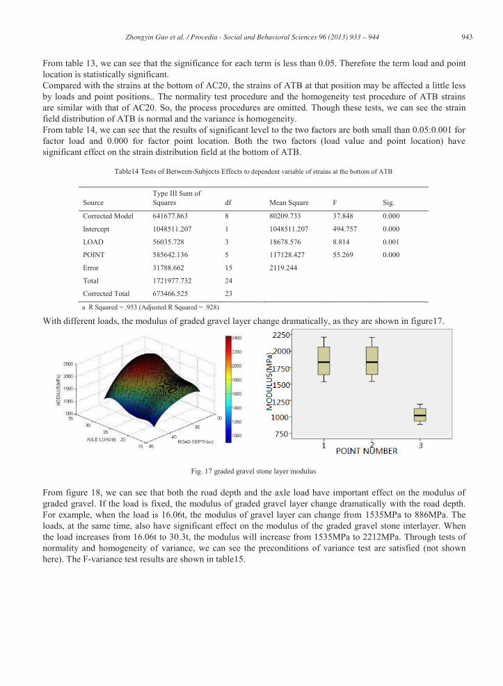
With different loads, the modulus of graded gravel layer change dramatically, as they are shown in figure17.
Fig. 17 graded gravel stone layer modulus
From figure 18, we can see that both the road depth and the axle load have important effect on the modulus of graded gravel. If the load is fixed, the modulus of graded gravel layer change dramatically with the road depth. For example, when the load is 16.06t, the modulus of gravel layer can change from 1535MPa to 886MPa. The loads, at the same time, also have significant effect on the modulus of the graded gravel stone interlayer. When the load increases from 16.06t to 30.3t, the modulus will increase from 1535MPa to 2212MPa. Through tests of normality and homogeneity of variance, we can see the preconditions of variance test are satisfied (not shown here). The F-variance test results are shown in table15.

944 Zhongyin Guo et al. / Procedia - Social and Behavioral Sciences 96 ( 2013 ) 933 – 944
Table 15 Tests of Between-Subjects Effects to the dependent variable of modulus
Source Type III Sum of Squares df Mean Square F Sig.
Corrected Model 2289710.500 5 457942.100 57.352 0.000
Intercept 29937843.000 1 29937843.000 3749.378 0.000
LOAD 486239.000 3 162079.667 20.299 0.002
POINT 1803471.500 2 901735.750 112.932 0.000
Error 47908.500 6 7984.750
Total 32275462.000 12
Corrected Total 2337619.000 11
From table 15, we see that both the load and the point depth have significant effect at statistical meaning on the modulus field of graded gravel stone interlayer.
5. Conclusions
From the analysis above, we can draw the following conclusions: (1) Strain model modified can predict the maximum bottom strains of asphalt layers exactly. (2) When the loads increase, the maximum strains at the bottom of AC20 and ATB do increase in value.
However, the shapes of strain distribution field do not change apparently. (3) The factors of load and point location have significant effect on the modulus of graded gravel stone
interlayers and on the strain distribution fields at the bottom of AC20 and ATB in statistical meaning.
Acknowledgments
This research is sponsored by Highway Bureau of Transportation Office, Shandong Province and it s highly appreciated
References (1) Bruce Daniel Steven. (2005).The development and verification of a pavement response and performance model for unbound granular
pavements. University of Canterbury. (2) A.A Van Niekerk . (2002), Mechanical behavior and performance of granular bases and sub-bases in pavements. Delft University Press (3) Uzan, J. (1985), Characterization of granular material. Transportation Research Record 1022 TRB (4) Erol Tutumluer.(2001),Characterization of granular materials subjected to complex static and dynamic loadings. University of Illinois
Urbana IL 61801 (5) Alex Adu-Osei. (2001).Characterization of unbound granular layers in flexible pavements research report sponsored by aggregate
foundation for technology. (6) Jayhyun kwon,(2007). Development of a mechanistic model for geo-grid reinforced flexible pavements, University of Illinois . Urbana,
Illinois (7) Tong Li.(2006). Investigation of unbound granular materials in flexible pavement. University of South Carolina. ProQuest Information
and Learning Company (8) Donald Mark Smith.(2000). Response of granular layers in flexible pavements subjected to aircraft loads. Louisiana State University.
Bell & Howell Information and Learning Company. (9) Amy L. Rechenmacher, Sara Abedi, Olivier Chupin, Andres D. Orlando.(2011). Characterization of mesoscale instabilities in localized
granular shear using digital image correlation. the International Workshop on Multiscale & Multi-physics Processes in Geo-mechanics, June 23-25, 2010, Stanford University.
(10) Corwin, E. I., Jaeger, H. M., & Nagel, S. R. (2005). Structural signature of jamming in granular media. Nature, 435, 1075 1078. (11) Einav, I. (2007a). Breakage mechanics Part I: Theory. Journal of the Mechanics and Physics of Solids, 55(6), 1274 1297. (12) Finno, R. J., & Rechenmacher, A. L. (2003). Effects of consolidation history on critical state of sand. Journal of Geotechnical and Geo-
environmental Engineering, ASCE, 129(4), 350 360.