The Statistical Analysis of Dose-Effect Relationships€¦ · Experimentation under laboratory conditions is ideal for the control of extraneous variation or possible bias. The experimental

CHAPTER 6

The Statistical Analysis of Dose-EffectRelationships

c. C. BROWN

Biometry Branch, National Cancer Institute, National Institute of Health.Bethesda. Maryland 20014. U.S.A.

6.1 INTRODUCTION. . . . . . . . . . . . . . . . . . . . US6.2 EXPERIMENTALDESIGN . . . . . . . . . . . . . . . . . U76.3 QUANTALRESPONSES. . . . . . . . . . . . . . . . . . 1206.4 MATHEMATICALMODELSOF TOLERANCEDISTRIBUTIONS. . . . . . 1226.5 ESTIMATIONOF A QUANTALDOSE-RESPONSECURVE. . . . . . . 1266.6 QUANTITATIVERESPONSES. . . . . . . . . . . . . . . . 1366.7 TIME-TO-oCCURRENCEMODELS. . . . . . . . . . . . . . 1366.8 APPLICATIONTO ECOLOGICALRISKASSESSMENT. . . . . . . . 1406.9 CONCLUSIONS. . . . . . . . . . . . . . . . . . . . 141

6.10 REFERENCES. . . . . . . . . . . . . . . . . . . . . 1426.11 APPENDIX: THE MAXIMUM-LIKELIHOOD METHOD OF FITTING

DOSE-RESPONSEMODELSTO QUANTALDATA. . . . . . . . . 145

6.1. INTRODUCTION

The relation of responses to doses of environmental toxicants is an importantelement in the control and prevention of ecological problems. In general terms,dose-response is the relation between any measurablestimulus, physical, chemical,or biological, and the response of living matter in terms of the reactions thestimulus produces over some range of the amount of stimulus. In toxicologicalsituations, there is normally, though not always, a monotone relation between theintensity of the stimulus and the particular responseit elicits.

The reactions to anyone stimulus may be multiple in nature, e.g. loss of weight,decrease in blood sugar, central nervous system disorders, decrease in organfunction, or even death. Each reaction will have its own unique relation with thedegree of the stimulus. In addition, the measurement of any specificreaction can bemade in terms either of the magnitude of the effect produced, including whetherthe effect is produced or not, or of the time required for the appearance of aspecific effect. These responsesmay be acute reactions, sometimes occurring withinminutes of the stimulus, or they may be long-delayedeffects such as cancer, whichmaynot appearclinically until most of the animal's normal lifespan has elapsed.

115

116 Principles of Ecotoxicology

Other responses may not even appear in the exposed subject, but may become

manifest in some later generation.The degree of stimulus, or in general teans, the dose level, may be measured in

different ways. For example, consider some animal that is exposed to a chemicaltoxicant in the environment, either through the air breathed, the food eaten, or

through 80me other external exposure. The magnitude of the stimulus, or exposurelevel, may be quantified as parts per million in the air or food, or may be measuredas the quantity of the substance actually reaching the target receptor, some internalorgan or other tissue. The former quantity can be thought of as the 'actual'exposure, or dose level, while the latter may be termed the 'effective' exposurelevel. The actual level may be modified by absorption, distribution, metabolism,detoxification, and excretion of the chemical substance. Therefore, the effectivelevel may well be some complex function of the actual level along with thebiochemical and physiological dimensions of the host resulting in a potentiallyquite different relation between the levels of the stimulus and the magnitude ofresponse, depending upon the manner in which the stimulus is measured. Swartzand Spear (1975) recommend relating the time-integrated internal exposure to theobserved response in carcinogenesis studies since mechanistic conclusions, which aredependent upon this relation, may be obscured by the relation of external tointernal exposure.

The relation between the dose level of a toxicant and the resulting reaction is

often impossible to estimate by direct measurements of the stimulus itself unless itsmechanism of action is known. A toxic element in different chemical constitutions

may produce quite different biological effects in the same host due to differentmodes of interaction with the organism and its tissues. Therefore, lacking completemechanistic knowledge, the relation between the toxicant and its effects on abiological system must be either observed in nature or tested in the laboratory orfield. Experimentation under laboratory conditions is ideal for the control ofextraneous variation or possible bias. The experimental conditions may be rigidlycontrolled and the results are subject to considerations of reproducibility. However,because of potential physical limitations of the laboratory, the experimentalconditions may well be unrealistic images of the natural environment and hence,extrapolation to the real world may be difficult and sometimes unwarranted.Experiments on plants or animals may also be conducted in the field. Here, the ideais to reproduce the natural environment as closely as possible, but with this type ofexperiment one cannot easily control the many factors which may have aninfluence on the results of the test.

This section is concerned with the statistical techniques used for the estimationof dose-response relations. It will be assumed that the particular agent in questionis known to be generally toxic and that the purpose of the following statisticalanalyses is to obtain an indication of the relation between dose level and the toxicresponse. The general methods are applicable to any experimental situation, be it ina highly controlled laboratory environment, in the field, or gradations in between.

The Statistical Analysis of Dose-Effect Relationships 117

One feature common to all experiments in any field, biological or other, is thevariability in the measured effects from a given stimulus. In experiments with livingmatter this variability will usually be much greater than in the common chemical orphysical measurements. In addition to the simple variation inherent in themeasuring device, such as a scale to measure weight or a more complex assay of theamount of a certain chemical in the blood, the response of the experimentalsubjects, be they plants or animals, may also be influenced by biological andphysiological factors such as sex, age, or some other physical conditions. The testsubjects themselves will not be a completely homogeneous group with respect to allimportant factors which may affect the stimulus-response reaction. The susceptibi-lities of the subjects to the stimulus may well be dependent upon geneticdifferences which, even if known, cannot be completely controlled. In anyexperiments used to estimate a dose-response relation, the results of theexperiment and its analysis must include some measures of the variability of theresults, for such results to be properly interpretable.

6.2. EXPERIMENTALDESIGN

The assessment of any stimulus-response relation will depend upon the data onwhich it is based. Inadequate data, whether experimental or observational,will notpermit estimation of this relation. As an extreme example, when the effect ismeasured in terms of the per cent incidence of a particular response, anyexperiment in which the dose levels are either too low to show any response, or sohigh that they all show 100%response, can obviously givelittle information on thedose-effect relation. Any study, properly designed to elicit adequate informationon the relation between dose and response, will entail the consideration of manyfactors (Emmens, 1948; Jerne and Wood, 1949; Finney, 1964).

The initial step is selection of the species of test subjects. Ideally, the subjectsshould be that species to which the results of the experiment are to be applied, or aclosely comparable species. If one wishes to estimate the toxicological effect ofsome chemical pollutant in the environment, then representative species in theenvironment, either terrestrial or aquatic or both, should be tested. However, thisapproach is often not feasible for a variety of reasons. The species to be testedshould be chosen on the basis of its susceptibility to the induction of the responseof interest and on the basis of its biochemical and physiological similarity to thespecies to which the experimental results are to be applied. Similar dose-effectrelations for many species will produce invaluable information on the generalapplicability of the dose-effect relation. Dissimilarities,which can be explained byknown physiological differences between the species, may also be useful forextrapolating from one speciesto another.

The next step in the experimental design is the selection of the route andduration of the exposure which should be comparable to those occurring in nature.An inhalation study cannot be extrapolated to oral exposure without making a


number of assumptions concerning the fate of the toxic agent between initial

exposure and its reaching the target tissue. Metabolic pathways or physiologicalbarriers may vary with different exposure routes. The results of single exposurestudies cannot always be applied to chronic exposures in the environment; a singledose of 100 units of some toxicant may be either more or less effective than 100

fractionated one-unit doses of the same agent distributed over a period of time. Forexample, Matsumura (1972) showed that the ratio of the chronic to acute oral

dosage for mallards required to produce 50% mortality is 50 for DDT and 1 fordieldrin and 'Zectran', with other insecticides falling within this range. In addi tion,single exposure situations may depend on physiological factors such as the age ofthe subject. Huggins et al. (1961) have shown that the rate of induction of

mammary cancer by 3-methycholanthrene in rats is strongly affected by the age ofthe animal at exposure.

The selection of dose levels for an experimental bioassay is a critical step in thedesign of the study and will depend upon the purpose of the study. If the primarypurpose is to show that a certain effect can be produced by the test agent, then theideal design would have one treated group at the highest dose level that can betolerated by the test subjects, i.e. a dose that will not produce other toxic effectsthat may obscure the response of interest. To guard against the possibility ofincorrectly using too high a level of the stimulus, a second, lower level is also

commonly incorporated in the design. If the response under consideration mayhave a spontaneous occurrence, then an untreated control group must also beincluded. This type of design will not, however, produce much information aboutthe shape of the dose-response relationship. An efficient design to ascertain thisshape should consist of a number of dose levels selected to produce a range ofresponse rates between 10% and 90%. If little or no prior information is availableon the expected response rates at various dose levels, then some type ofpre-experiment should be performed. Dixon and Mood (1948) proposed what hasbeen termed an up-and-down method, using single-test subjects, to estimate thedose level required to produce a specific response rate of some acute effect. Their

technique has been generalized and extended by Robbins and Munro (1951) andHsi (1969) to estimate the dose levels that produce 10%,50%, and 90% responses;the final dose-response bioassay study can then be designed to use dose levelswithin this range. Bartlett (1946) suggested the use of an 'inverse sampling rille' forthis problem. Ideally, the more dose levels used, the better the dose-responserelationship can be estimated, but the cost of the study will normally determine thetotal number of subjects in the experiment. Therefore there is some trade-offbetween having many dose levels and having adequate numbers of test subjects ateach dose.

The optimal spacing between the chosen number of dose levels is unknown, buta common approach is to choose equal spacing on the dose-level scale that is to beused in the analysis. For example, if it is planned to use a probit or log-logisticmodel for the analysis, then the doses should be selected to have equal spacing on a

The Statistical Analysis of Dose-hYfect Relationships 119

logarithmic scale. Hoel and Levine(1964) have givenan optimal spacingsolution tothe general polynomial regressionproblem when the purpose is to estimate a valueoutside the observation range.Wetherill(1963) givesan optimal spacingfor use in alogistic model.

Once the total number of test subjects has been decided, a decision must bemade as to their allocation over the dose levels; this will depend upon the purposeof the study. If the design calls for k dose-levelgroups, each to be compared to acontrol group simply to frod if an effect of treatment exists at some dose, then anoptimal design is to allocate an equal number, say Nt, to each treated group, andplace ykNt subjects in the control group. However,if the purpose is to estimate theresponse at each dose level equally well, then the number of subjects allocated tothe ith level should be proportional to Pi(1 - Pi)' wherePi is the expected responserate. This means that one should allocate progressivelyless subjects to the extremedose levels, both low and high. However, this does not imply that the number ofcontrol subjects should be zero unless the unexposed response rate is known to bezero. If no prior information exists on the expected response rates, then equalallocation should prove a reasonable strategy.

More complex bioassays involving combinations of toxic agents or theexamination of different factors that modify the effects of a single toxicant mayalso be designed. The combined exposure to different toxicants may produceindependent, additive, or synergistic effects, or they may be antagonistic to oneanother. Definitions of these actions, and the construction of theoretical models toexplain them have been proposed by many authors; Plackett and Hewlett (1967),Hewlett and Plackett (1959, 1964), and Ashford and Smith (1964, 1965) areamong them. Street et al. (1970) discuss the ecological significance of suchinteractive effects and the complexities inherent in their measurement. The subjectis also discussedin Chapter 9.

A single experimental bioassay can measure the effect of a stimulus under onlyone fixed set of experimental conditions. However, nature presents more than asingle face, and the ability to extrapolate experimental results to the naturalenvironment will depend upon the generality of the bioassay design. Muirhead-Thompson (1971) discusses the influence of physical factors, such as temperature,water hardness, and pH, on the pesticide impact on fresh water. Matsumura (1972)showed that the mortality rate of brine shrimp exposed to various chlorinatedhydrocarbon insecticides was dependent upon the salt concentration, the effectbeing greatest at either extremely low or high concentrations. Therefore, since wedo not know whether these potential modifying factors exert independent orinteractive effects, multifactorial studies should be designedin such a manner as toallow for the measurement of all possible joint effects. A complete multifactorialexperiment will normally require a sizeable study. For example, a study with 3factors having 4, 3, and 2 levels respectivelyalong with 5 dose levelswould require120 =(4 x 3 x 2 x 5) groups of test subjects. At twenty subjects per group, wewouldbe facedwith an experiment containing 2,400 subjects. However, using


experimental design techniques as described by Kempthorne (1952) and Cochran

and Cox (1957) for general statistical problems and Finney (1964) and Das andKulkarni (1966) for bioassays, the size of these studies may be reduced if one iswilling to assume that certain interactions between the factors, the dose and theresponse are negligible. However, this reduction in experimental units producesgreater complexity in the analysis of such studies, so great care should be exercisedin their design.

6.3. QUANTALRESPONSES

One type of response commonly measured in toxicologicalstudies is the quantal,or all-or-nothing, response, e.g. death. Measurements of degree of effect willnormally provide a more refmed measure of the response to a stimulus, butquantification is often very difficult or, for some responses,impossible.

When the response is quantal, its occurrence, for any particular subject, willnormally depend upon the degree of the stimulus. For this subject, under constantenvironmental conditions, there will usually be some level of the stimulus belowwhich the response will not occur and above which it will. This level is referred toas the subject's tolerance. Because of the biological variability among thepopulation of individuals, their tolerance levels will also vary, sometimes withinquite wide limits.

For quantal responses it is therefore natural to consider the distribution oftolerances over the population in question. If D represents the dose level of aparticular stimulus, then the distribution of tolerances may be mathematicallyexpressed as f(D)dD which represents the proportion of individuals havingtolerances between D and D + dD, where dD is small. If we are willing to assumethat all members of the population will respond to a sufficiently high level of thestimulus, then the sum of these proportions should equal unity, or

f~ f(D)dD = 1. (6.1)

If a population is exposed to a dose of Do, then all members with tolerances lessthan or equal to Do will respond, and the proportion they represent of the totalpopulation can be calculated as,

fDO

P(Do) , f(D)dD.0

(6.2)

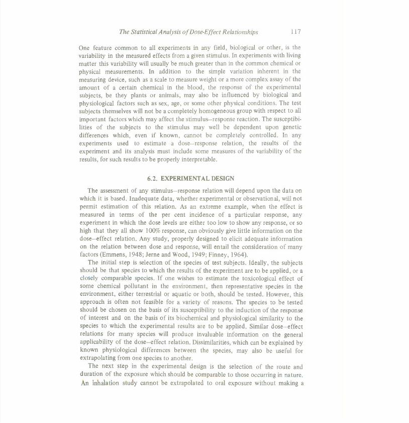
Figure 6.1 shows a hypothetical tolerance distribution, f(D)dD, along with itscorresponding cumulative distribution, P(JJ), as defined in equation (6.2). ThefunctionP(D) represents the dose-response relationship for the population whenthe response is quantal in nature. For any individual, the dose-response curvewould be a step function, zero less than its tolerance and unity greater than itstolerance. However, for a population of individuals, the response can be measured


1.0

0.8

(:)z15z~ 0.6(/)wII:

Z0

~ 0.40c..0II:c..

~ ~/~------

./~~~//~ --"~ f(D;8)-

0.1 1.0 10.0

DOSE LEVEL

Figure 6.1 Example of relation between thres-hold distribution f(D) and dose-reponse curveP(D)

as the proportion responding. The curve defined by P(D) can also be consideredasthe probability that one individual, selectedat random from the population, willrespond to a dose level D. This particular distribution in Figure 6.1 assumesthatP(O) = 0 (no respondersfor azero dose)and P(oo)= 1 (all will respond to somehighdose). Either or both of thesetwo assumptionsmay be untrue. The first assumesnospontaneous occurrence of the particular responsewhich is false for a number ofresponses,while the secondmay be false if either an immune group exists withinthe population or the particular responsein question becomesoverwhelmed at highdose levelsby a different response and does not have a chanceto becomemanifest.

If a group of N test subjects were chosen at random from some populationhaving a tolerance distribution given by f(D)dD, and each subject was exposed tothe same dose level D, then the number of subjects showing the response would bea random variable having a bincmial probability distribution. In mathematicalterms, the probability of R responders out of N subjects each givena dose of D, isgiven by,

probeR)=(~)P(D'fQ(Dt'-R,(6.3)


where Q(D) = 1 - P(D) and P(D) is the probability of response for one randomly

chosen test subject as defined in Equation 6.2. The observed proportion ofresponders in the test sample, p(D) = R/N, is then an estimate of the trueproportion in the population, P(D). This observed proportion can be either larger orsmaller than the population value because of sampling variation, but the variation iscentered around the value P(D) and decreases as the size of the test sampleincreases.

An estimate of the dose-response relation can be obtained by testing variousgroups of subjects at different dose levels. Each value of the observed proportion ofresponders, p(D), is an estimate of its corresponding P(D), and from thesequantities, the population cumulative tolerance distribution can be estimated. Ingeneral, P(D) will increase with the dose D, but if the number of test subjects ateach dose level is small, then sampling variation may interfere with the regularity oftrend in the observed proportions p(D).

The preceding discussion has assumed that the subjects chosen to be tested ateach dose level have been randomly selected from some larger group of subjects andthat the experimental conditions are the same for each dose. Deviations from theseassumptions, either by choice or by chance, may result in the binomial modelequation (6.3) being inapplicable. For example, non-random selection of testsubjects, such as different age groups at the different dose levels or the selection ofa group of subjects from the same parent to be tested at the same dose, would causethe ratio of the variation among dose groups to the variation within groups to belarger than expected under the binomial model. In addition, differences betweenthe dose groups with respect to factors known to be associated with the response,such as age, sex, weight, or some conditions of the experiment itself, could producean undesired bias in the observed proportions. In any experimental situation, caremust be given to select the groups at random and to control other variables of theexperiment.

6.4. MATHEMATICAL MODELS OF TOLERANCE DISTRIBUTIONS

A toxicological dose-response experiment, or bioassay, will result in a series ofdose levels, Di, i = 1, . . . , k, along with their corresponding observed proportionsresponding, Pi = p(Di). These pairs of values (Dj, pD provide an estimate of thedose-response relation for only a limited number, k, of dose levels. An estimate ofthe entire dose-response curve can be made only by assuming some generalfunctional form relating dose to response, i.e. P(D) = g(D; 8), where the function g

represents some particular class, the member of the class being defined by theunknown constant, or constants, 8. For example,g may be a simple linear function,g(D; 8) = 80 + 8 ID, or a more complex function such asg(D; 8) =1/2 + (l/1T)tan-l(80 + 81 log (D)).

The results of toxicity tests often show that the observed proportion ofresponders monotonically increases with dose and shows a sigmoid relation with


some function of the exposure level.This led to the development of the normal, orprobit, model of the dose~tolerance distribution. This model assumes that thepopulation distribution of tolerances is givenby the normal probability model,

[I

[

xeD) - 80

]

2

]feD; 8) =(21T8D-1/2exp - 2 8 I ,81> 0(6.4)

orx(D)-Oo

J0,

P(D;8)= -00 (21T)-1/2exp(-!t2)dt,

where xeD) = x is some transformed value of the dose levelD. Some transforma-tions commonly used in practice are

x =logl 0 (D),

and, more generally

x =fYl,

where a ~ 1. The validity of any transformation will depend upon the mechanismof the response to the stimulus in question and, as such, is beyond the scope of thisdiscussion. We, as Finney (1949), propose to use any transformation that appearsto fit the observational data, but any additional mechanistic knowledge for aparticular problem should be incorporated into the model. The normal model inequation (6.4) has commonly been used with the logarithmic dose transformation.A history of the development of this model is givenby Finney (1952).

Other mathematical models of tolerance distributions which lead to the sigmoidappearance of their corresponding dose-response curvesare:

1. The logistic curve,

P(D; 8) = {1 + exp [10g(80)- 8110g(D))}-1, 80, 81> 0

DO,

- 80 + DO,(6.5)

which is derived from chemical kinetic theory and was proposed by Wilson andWorcester (1943) and Berkson (1944) for bioassay analyses,and

2. The sine curve,

P(D;8) =H 1 + sin[80 + 8 llog(D)]} (6.6)

which is applicable only over a limited range of doses, -1T/2 ~ 80 + 8llog(D) ~ 1T/2,and has no theoretical justification other than computational simplicity (Knudsenand Curtis, 1947). Other dose-response models have been proposed on the basis ofwhat has been called 'hit theory'. These models do not start with an assumeddose-tolerance distribution to produce a dose-response curve, but are derivedon


general mechanistic dose-response assumptions. Turner (1975)summarizes allthese models. The more commonly used models are the singlehit model,

P(D; 0) = 1 - exp(-OD), 0>0 (6.7)

and the multi-hit model,

m-l 1P(D;O)= 1- ~ I" (OD)h exp(-OD),h=O h.

0>0 (6.8)

where m is the minimum of 'hits' on a receptor required to obtain a response.Another model, which has been proposed as a mechanism in carcinogenesis,hasbeen termed the multi-stage model. One derivation of this general process, due toArmitage and Doll (1961) and extended by Peto (1975), leads to the mathematicalrelation,

P(D; 0) = 1 -exp (- ~ OhDh),h=l

0h ;;. 0, h = 1,..., m (6.9)

where m is the number of stages in the process affected by the agent. Adose-tolerance distribution may be obtained from these models by invertingequation (6.2), i.e.

feD; 0) = dP(D; 0) (6.10)

Therefore, the tolerance distribution corresponding to the multi-hit model (6.8) isthe gammadistribution

Om

f(D;O) = f(m) Dm-l exp(-OD)(6.11)

which looks similar to both the log-normal and log-logistictolerance distributions.Table 6.1 compares the dose-response relations of three models. It might be

thought that the selection of one particular model over the others would be obviousfrom inspection of the calculated responses but this table shows that three of themost commonly used models, log-normal,log-logistic,and single-hitgiveresults thatdiffer by little over a 256-fold dosage range (FDA Advisory Committee onProtocols for Safety Evaluation, 1971). It would take an inordinately largeexperiment to be able to conclude which of the three models best described theobservational data.

If the calculated dose-response curve is to be used to estimate the response ratethat would be expected from an exposure level within this range of observableresponses, then all three models will givecomparable results. Interpolation betweenobserved data points within the range of approximately 50/0-95%response rates willnot be greatly affected by the mathematical model selected. However, extrapola-

tion to exposure levelsexpected to givevery low response rates is highly dependentupon the choice of mathematical models, which is shown in Table 6.2 extendingthe previous table to much smaller doses. It can be seen that the further oneextrapolates from the observed response range, the more divergent the variousmodels become. At a dose level that is 1/1000 of the 50% response dose, thesingle-hit model gives an estimated response rate 200 times as large as thelog-normal model. The fact that a moderate-sized experiment conducted at doselevels high enough to give observable response rates cannot discriminate amongthese various models, and the fact that these same models show a substantialdivergence at small dose levelspresent major difficulties for low dose extrapolationproblems. Brown (1976a) has suggested the use of a multi-stage model (equa-tion 6.9) along with an estimate of both sampling and model variability for thisproblem, since the multi-stage model has the extrapolation characteristics of mostother models, depending upon the number of stagesused.

It should be noted that all the mathematical dose-response models presentedhave the feature that for any dose D> 0, P(D) > 0, i.e. there is no absolutethreshold level below which the probability of response is zero. A common

Table 6.2 Expected Per Cent Responding atLow Doses for Models Describing ObservedResponses in the 5%-95% Range Equally Well

The Statistical A 11lllysisof Dose-Effect Relationships 125

Table 6.1 Expected Per Cent Responding forVarious Models over a Range of Dose Levels

Dose Log-normal Log-logistic Single.hitlevel model model model

16 98 96 1008 93 92 994 84 84 942 69 70 751 50 50 501 31 30 29"21 16 16 1641 7 8 881 2 4 416

Dose Log-normal Log-logistic Single-hitlevel model model model

0.01 0.05 0.4 0.70.001 0.00035 0.026 0.070.0001 0.0000001 0.0016 0.007


toxicological problem is whether or not a threshold levelactually exists. Thresholdsshould, however, be considered from two different viewpoints: a 'theoretical' levelbelow which a toxic response is impossible; and a 'practical' levelbelow which thechance of response is highly unlikely or unobservable.Theoretical thresholds couldvary substantially in an outbred population due to genetic differences, and theirexistence cannot be proven by statistical arguments; this proof would have to comefrom complete knowledgeof the mechanismof toxicological action.

Experimental or observational evidence for the existence of a threshold iscommonly presented in the form of a dose-response graph in which the responserate is plotted against dose level. Either the existence of doses not showing anincrease in response over controls or the extrapolation of such curves to low doseswhich apparently would result in no increased response are cited as indications ofthe existence of some threshold below which no response is possible. This type ofevidence is of little value. In the first situation, the observation of no respondersdoes not guarantee that the probability of response is actually zero. From astatistical viewpoint, zero responders out of N at risk is consistent at the 5%significance level, with an actual response rate between zero and approximately3/N.

In the second case, when a graph of observed dose against responses isextrapolated downward to a no-effect level, the observed dose-response relation,often linear, is assumed to persist throughout the entire range of dose levels. Thisassumption can easily lead to an erroneous conclusion when the true dose-responsecurve has a rising slope, i.e. is convex. Brown (1976b) discusses this problem indetail when the responseis carcinogenicin nature. He shows that statistical analysesof bioassay results cannot discriminatebetween mathematical models which assumethe existence or non-existence of an actual threshold. Therefore, without aknowledge of the mechanismproducing the response, when extrapolating below theobservable response range, it would be prudent to assumethat no threshold exists.

6.5. ESTIMATIONOF A QUANTALDOSE-RESPONSE CURVE

In this section we shall assume that we have concluded a typical quantaldose-response experiment, or bioassay, and, having observed the proportionsresponding at various dose levels, we wish to estimate the population dose-response relation.

First we have to select one of the mathematical models with which we shallperform the analysis. For the sake of simplicity,we shall use the log-logisticmodel(equation 6.5), though the general technique to be described is applicable to anymodel. The logistic model can be written as,

P(x;a,b)={1 + exp[-(a +bX)]}-I, b;;:'O (6.12)

where P is the probability of a randomly selected individual from the populationresponding to an exposure of x =logedose). The series of log dose levels are denoted


as x" X2, . . . , Xk and their corresponding observed proportions responding asPi =P(Xi)='dni' i = 1,2, . . . , k, where'i is the numberof test subjectsrespondingout of ni exposed at the ith dose level. The estimation of the dose-response curveconsists of estimating the two unknown parameters a and b, which can beaccomplished in a variety of ways, ranging from simple graphical techniques(DeBeer, 1945; Litchfield and Wilcoxon, 1949), to more sophisticated methodssuch as maximum likelihood or minimum chi-square. The maximum-likelihoodmethod is an extremely general, fully efficient estimation technique but iscomputation ally difficult (Cornfield and Mantel, 1950). Bliss (1935) and Finney(1952) give its application to the probit model and the details of this method aregiven for any general quantal response model in the Appendix to this chapter. Asimpler computational approach has been given by Grizzle et al. (1969) forthe generallogistic model and by Berkson (1949) for bioassay data.

The logisticmodel in (6.12) can be rewritten as,

[p(Y.:;a, b)

]= a + bx

log Q(x;a, b)(6.13)

whereQ(x;a, b) = 1- P(x;a, b). The transformation 10g(P11- P) has been termedthe logit transformation by Berkson (1944). This has reduced the problem from anon-linear to a simpler linear problem which can be solved by the method of leastsquares. The linear model in equation (6.13) relates the response to the dose for theith experimental group as,

Zi =a + bXj

where Zj is the logit of the response rate, and Xj is logarithm of the dose level.Since the variances of the observed logits are not necessarily equal, we should

properly use weighted, as opposed to unweighted, least squares. The variance ofthe ith response rate is PjQi!ni, where Qj = 1 - Pi and Pj is the population responserate. From asymptotic statistical theory, the variance of the logit of the responserate is l/njPjQi, which is an approximate variance for finite samples. Therefore, theweighted least squares method uses Wj =n;>iQi as the weights, which can be

approximated by the observed response rates Wj =niPjqj. In the event thatpj = 0 or1, which would result in the weighting factor being zero, Berkson (1953) suggestsusing Pi = 1/2nj in place of zero, and pj = 1 - 1/2nj in place of unity. The weightedleast squares technique produces the following estimates for a and b,

LW'Y~LW-Z'- LW'X'LWY'Z' .. - ..."' , , " ..."" - b-a - 2 2 =Z - X,

LWjLWjXj - (LWjXj)

and (6.14)

. LW'LW'X'Z' - LW-Z'LW-X' LW' (X. -x )(z. - Z)b = ' " I I I I ,= " I

~W'~W.Xf - (~w.x. )2 ~w. (x.-i )2'

, " , , , ,


where x = ~wixd~wi and z = ~WiZi/~Wi'Oncea and b are estimated, thepopulation response rate can then be estimated for any dose level D in thefollowing manner. First estimate the logit of the response rate usingequation (6.13),

i = Ii + b log(D),

and then transform the logit to the response probability using equation (6.12),

P(D) = (1 + e-zrl

The estimated variances of these parameter estimates are given by,

2 - ~WiXJ - ~WiXJ /"E,WiSa - 2

(~

)2 - ~

(- 2 '

"E,wi~WiXi - ",",WiXi ",",Wi Xi - X)

and (6.15)

2 - ~Wi - 1Sb - ~ 2

(~

)2 - ~ (

-)

2",",Wi"E,WiXi- ",",WiXi "'"'WiXi - X

The variance of the estimated logit z of the response rate for any value of the logdose,X = 10g(D),can be obtained from the relation,

Var(z) = Var(a + bX) = S~ + x2sl + 2XS~b,

where S~b = - X/"E,wi(Xi- X)2 is the covariance between the two parameterestimates, aand b. This can be simplified to become,

1 (X - X)2( ) S2 - - +

)2Var z = Z - "E,Wi "E,Wi(Xi-X

(6.16)

This variance can be used to place statistical confidence limits on the estimatedlogit,

z :t Zti/2Sz (6.17)

where Zti/2 is a standard normal deviation corresponding to a total tail area of Q.For 95% confidence limits, Q = 0.05 and Zti/2 = 1.96. Once these limits are placedon the estimated logit, they can be transformed by equation (6.12) to giveconfidence limits on the estimated population response,

{1 + exp [- (z - Zti/2Sz))} -I <. P(D) <. {1 + exp [- (z + Ztif2Sz)] }-I (6.18)

The regression equation (6.13) can also be used in reverse to fmd that dose levelwhich is expected to produce a certain population response rate. A commonmethod of characterizing the toxicity of a stimulus is by means of the medianeffective dose. This value is defined as the dose which will produce a response inhalf the population, and thus is sometimes called the median tolerance. This median


effective dose is commonly denoted by EDs o. When the response in question isdeath, then the term LDs 0, the median lethal dose is used. Analogous symbols maybe denoted dose levels which affect other proportions of the population, such asthe ED 10, the dose which causes 10% of the population to respond.

In general, an estimate of the EDp, the dose resulting in a proportion p ofresponders, can be obtained from equation (6.13) as,

Xp = 10g(Dp) = (log(p/q) - a)/b

The approximat€; variance of this log dose is given by,

(6.19)

2 '- 2

s} =(l) (~ + (Xp - x) ).p .b ~Wi ~Wi(xi - X)2

As can be seen from this expression, the variance of this log dose increases as theestimated log dose moves away from the average log dose of the experiment. As

before, confidence limits for the dose Dp giving the desired response rate p can beobtained from equations (6.19) and (6.20) as,

(6.20)

exp(~ - ZOI./2SXp)';;;; Dp .;;;;exp(Xp + ZOI./2SXp)(6.21)

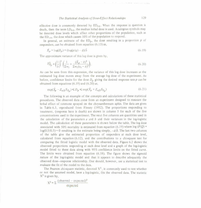
The following is an example of the concepts and calculationsof these statisticalprocedures. The observed data come from an experiment designed to measure thelethal effect of rotenone sprayed on the chrysanthemum aphis. The data are givenin Table 6.3, reproduced from Finney (1952). The proportions responding totreatment, (response here is death) are shown in column 5 for each of the fiveconcentrations used in the experiment. The next fivecolumns are quantities used inthe calculation of the parameters a and b and their variances in the log-logisticmodel. The calculation of these parameters is shown below the table. The log doseassociated with 50% mortality is estimated from equation (6.19) where log (P/Q) =log(0.5/0.5) =0 resulting in the estimate being simply, -0/6. The last two columnsof the table give the estimated proportion of responders at each dose level,calculated from equation (6.12), and the contributions to a chi-square test forcomparing the fitted logistic model with the observed data. Figure 6.2 shows theobserved proportions responding at each dose level and a graph of the log-logisticmodel fitted to these data along with 95% confidence limits on the fitted curve.The limits were obtained from equation (6.18). The figure shows the sigmoidnature of the log-logistic model and that it appears to describe adequately theobserved dose-response relationship. One should, however, use a statistical test toevaluate the fit of the model to the data.

The Pearson chi-square statistic, denoted X2, is commonly used to test whetheror not the assumed model, here a log-logistic,fits the observed data. The statisticX2 is givenby,

2 (observed - expected)2X =~expected

Table 6.3 Example of Log-logistic Model Applied to Quantal Response Data. Toxicity of Rotenone. (Reproduced by per-mission of Cambridge Univ. Press from Finney, 1952)

wxz

Estimatedproportion Chiresponding square

-10.055- 9.863

1.64521.95924.423

28.109

0.1290.3220.5390.8050.907

0.0360.0270.0540.8440.432

- ~wx =1.615x= ~w

- - ~wz = 0.113z - ~w

~WX2S~= = 0.406

(~w~wx2 - (~WX)2)

~wS~= = 0.146

(~W~wx2 - (~wx)2)a =z - bx= -4.838

(~w~wxz - ~wz~wx)- = =3.065b (~w~wx2 _(~WX)2)

-iiXs 0 = --,:-= 1.578b

LDs 0 = 4.85

95% confidence limits on LDso: 4.37';;; LDso';;; 5.37

2X(3) = 1.393

Concen-tration Log Number Proportion(mgfl) dose Responders at risk respondingD x r n p w =npq wx WX2 wz

2.6 0.956 6 50 0.120 5.380 5.048 4.826 -10.5183.8 1.335 16 48 0.333 10.661 14.232 19.0 - 7.3885.1 1.629 24 46 0.522 11.477 18.696 30.456 1.0107.7 2.041 42 49 0.857 6.007 12.260 25.023 10.759

10.2 2.322 44 50 0.880 5.280 12.260 28.468 10.518

38.705 62.496 107.773 4.381

0.06-1f2J0

L5

CONCENTRATION (mg/l)

Figure 6.2 Estimated dose-response curve with 95%confidence limits (rotenone toxicity example). (Repro-duced by permission of Cambridge Univ. Press fromFinney, 1952)

which, for this type of bioassay experiment, is equal to,n.

X2= L{"::-:- (Pi '- Pi)2PlJ;

where Pi is the estimated response probability for the ith dose level,and qi = 1 - Pi'The degrees of freedom for this statistic are given by the number of dose levelsminus 2, the number of parameters in the mode] that were estimated from the data.For this example, the tables show that X2= 1.39 with three degrees of freedom,which is not statistically significant. Therefore, we may conclude that the modeladequately fits the observed data,

This is not always the case, however, as shown in the following example. Thedata are from an experiment by Sinnhuber et al. (1968) in which Rainbow trout,held in 200-gallon tanks, were fed with different commercial diets plus additives.The amount of aflatoxin in the diet and additiveswasmeasured and the response ofinterest was the incidence of hepatomas. The fish were sampled at 6, 9, and 12months. Tabb 6.4 shows the results of the 12 month sample.

The last column of the table, the chi-square calculation to test the adequacy ofthe log-logisticmodel, yields a chi square of 21.9 with 8 degreesof freedom whichis statistically significant, P < 0.01. An examination of the standardized differencesbetween the observed and expected proportions responding, givenby

(6.22)

Pi - Pi

Rj = ...t .fr./n.Pt'll I

(6.23)


tOr/'

--/'

/0 -

0.8/ -- --

t9 OBSERVED DATA 0/ '"

Z / '"

15 / /

/ /Z /0 / /a.. 0.6 / /(/) / /w /a: /Z

/ /0

/ /0.4

/ // /a: / /0

a.. / /0

/' //'a: /' ./a.. 0.2 ./ /'

.//'

././

Table 6.4 Example of Log-logistic Model Applied to Heterogeneous Quantal Data. Incidence of Hepatomas in Rainbow TroutFed Diets Containing Aflatoxin for 12 Months. (Reproduced by permission of the authors from Sinnhuber et al., 1968)

aped for 13 months.

kWX kWZx = -= 2.515 Z = -= 0.827

kW kW

kwx2 kWZ - kWXkWXZ)a= =-1.912

(kWkwx2 - (kWX)2)

(kWkWXZ - kWZkWX)b =- 2 = 1.089

(kWkWX2 - (kWX) )

kWX2S~ = .= 0.255

(kWkwx2 -(kWx)2)

2 kWSb 2 0.037(kWkwx2 - (kWX) )

Concen-tration Log Number(ppb) dose Responders at riskD x r n

0.8a -0.223 0 123.7 1.308 5 104.0 1.386 2 135.0 1.609 9 187.9 2.067 5 128.0a 2.079 20 30

15.3 2.728 62 8219.0 2.944 34 3936.5 3.597 31 4042.0 3.738 89 90

Proportion Estimatedresponding proportion Chip W =npq wx wz wx2 wxz responding square

0.0 0.444 -.099 -1.429 .022 0.319 0.104 1.3930.5 2.5 3.27 0.0 4.277 0.0 0.380 0.6110.154 1.907 2.643 -2.910 3.663 -4.033 0.401 3.3020.5 4.5 7.241 0.0 11.651 0.0 0.460 0.1160.417 2.929 6.054 -0.908 12.514 -1.877 0.584 1.3780.667 6.720 13.970 4.495 29.044 9.346 0.587 0.7920.756 15.251 41.604 17.005 113.496 46.388 0.742 0.0840.872 4.625 13.616 8.492 40.086 25.0 0.785 1.7490.775 7.121 25.613 8.538 92.130 30.710 0.881 4.2870.988 1.459 5.454 5.966 20.387 22.301 0.896 8.175

47.456 119.366 39.249 327.270 128.154

X?S)=21.887


may sometimes give a clue as to where the assumedmodel fails. Draper and Smith(1966) give an excellent discussion of residual analysis. In this situation, thereappear to be no systematic deviations related to dose levelnor to response rate, sowe would have to conclude that the assumption of binomial samplingmay be inerror. The variation in the data is larger than would be expected under the binomialassumption. The original experiment consisted of 15 groups being fed various dietscontaining different amounts of aflatoxin. This variation in diets and additivesmaywell have created the extra sampling variation. Kleinman (1973) and Cochrai"i(1943) discuss this problem of proportions with extraneous variation from theviewpoint of statistical tests in the analysis of variance. They consider the extravariation to be additive to the binomial samplingvariation. Finney (1952) suggestsassuming that the true variation is simply a multiple of the binomial variation, andhe proposes multiplying each of the variance estimates in equations (6.15), (6.16),and (6.20) by a heterogeneity factor, X2/k, where k is the number of degrees offreedom for the chi-square statistic X2. In addition, in order to allow for theuncertaintly in estimating this heterogeneity factor, the normal deviates,Ze</2,usedin calculating confidence limits, equations (6.17) and (6.21), should be replacedbyt values, tk,e</2where t has k degrees of freedom. Since these t values are largerthan the corresponding normal deviations, this has the effect of producing widerconfidence intervals. In the previous example with heterogeneous data, the 95%confidence limits on the probability of response at a concentration of 5.0 p.p.b. ofaflatoxin in the diet would be, using no heterogeneity factor and using normaldeviations,

0.35 ~p(5 ppb) ~ 0.571

However, after multiplying the variance in equation (6.16) by the heterogeneityfactor 21.887/8 = 2.736, and using a t value with 8 degrees of freedom, 2.306, inequation (6.18), the proper 95%confidencelimitsbecome,

0.264~P(5 ppb)~0.669

which are substantially wider than those calculated assuming no heterogeneity. Itshould be noted, however, that this correction procedure is only an approximationand should not be used if the Pearson X2statistic is not statistically significant.

The preceding results have been obtained by tacitly assuming that no responsewas possible at a zero dose, i.e. P(O) =O. This is seen to be true for the log-logisticmodel defined in equation (6.12). When the dose is zero, the log dose, x, is minusinfinity, and since the parameter b is restricted to be non-negative,the probabilityof response becomes zero. This assumption of no response for no stimulus will notnecessarily be true. In the two previous examples, both experimental designscontained a control, non-treated, group which produced no responders, so therewas no apparent reason to consider the possibility of spontaneous, non-dose-related, response. However, if the response under consideration is one which eitherappears among a group of untreated subjects, or if such controls are not available,it

--- --


may be expected to have a spontaneousoccurrence,then any mathematicaldose-response model should properly allow for this possibility.

Two methods have been proposed to incorporate the possibility of response dueto factors other than the stimulus in question. The first is known as 'Abbott'scorrection', attributed to W.S. Abbott (1925), and is based on the assumption ofan independent action between the stimulus and the background, or spontaneousresponse. If a proportion C of the subjects would respond in the absence of anystimulus, then the total response rate at a dose level D, assuming independentactions, would be,

1"(D) = C + (1 - C)P(D) (6.24)

From this equation it follows that the proportion responding due to the stimulusalone is,

P(D) = (1"(D) - C)(1 - C)

(6.25)

If the spontaneous response rate C were known exactly, then the previouslog-logistic model could be used with only minor modifications. The observedresponse rates P; should be transformed to their corresponding dose-relatedresponse rates Pi by use of equation (6.25). These Pi would be transformed tologits, log(p/l - p). The weights wi used for the calculation of the parameters a andb, and their variances, become,

W~= niPi (1 - Pi)I

l+-C-Pi (1 - C)

(6.26)

which are equal to wi when C =O. These modifications should not add unduecomplexities to the estimation of a dose-response curve. However,the spontaneousresponse rate is usually unknown, and even the knowledge of the proportionresponding in some control group will only provide a range of plausiblespontaneous rates. In this common situation of uncertainty, more complexmethods of estimation, such as maximum likelihood, will be required and thegeneral technique described in the Appendix to this chapter can be applied.

The second method of allowing for the spontaneous occurrence of response wasproposed by Albert and Altshuler (1973) in which they suggested that the naturalenvironment contains some additive background level of the stimulus, Do, so thatthe response rate for a dose D would be,

P'(D) = P(D + Do) (6.27)

Abbott's correction factor would then be givenas C =1"(0)=P(Do).Therefore,if Cand the true dose-response curve were known, the background levelDo could alsobe computed. This method, which will giveresults similar to the previous approach,


can only be employed using more complex estimation procedures. The maximum-likelihood method, assumingthat Do is an unknown parameter, can be used.

In general, when the response under consideration may have a spontaneousoccurrence independent of the stimulus, one should take care when using a modelthat assumes no such possibility. Figure 6.3 shows the effect of a spontaneousoccurr~nce on the log-logisticdose-response function. The probability of responseis given by equation (6.24) where P(D) is the log-logisticmodel. The figure showsthat, on a logit scale, whereas the log-logisticmodel is a linear function of the logdose (equation 6.13), the addition of a spontaneous response (here C =0.05)induces a curvature at the low response rates. This could produce a bias inestimating the parameters of the log-logistic model assuming no spontaneousoccurrence. The model from which the 'true' curve was produced has parametersa =-5 and b = 3, but the straightlinefittedby eyethroughthis'true' curvewouldestimate them as fi =- 3.2 and & = 2. In general,when the 'true' dose-responsecurve contains a spontaneous element, then any model which assumes no suchpossibility will lead to an underestimate of the slope and an overestimate of theintercept. Looking at the difference between the estimated and 'true' curves inFigure 6.3 shows this difference to be negative for low dose levels, positive formoderate dose levels, and negative for high dose levels. This pattern provides auseful clue when examining the standardized residuals from the fit of a model toexperimental data.

0.9

wenz0c..enwa:u.0

~::iii'i«II)0a:c..

0.5~ ESTIMATED DOSE - RESPONSE ~~=-3.2,b=2 /,..'"'",..

,../'" /- TRUEDOSE- RESPONSE,..'" / a=-5, b=3, c=O.05

'"'"

'"'",..,../-

0.1

,..'"

0.031 2 4 6

DOSE LEVEL

Figure 6.3 Comparison of true dose-response curvehaving spontaneous occurrence with estimated curve assum-ing no spontaneous occurrence


6.6. QUANTITATIVERESPONSES

The preceding discussion has been concerned only with quantal responses. Inmany biological investigations,however, it is possible to quantify the magnitude ofthe response. Such data could be reduced to the quantal form by a simpledichotomy of the measurements into those greater than or less than some selectedvalue. Since this procedure is wasteful of information, it would be better to use theactual measurements to construct a dose-response relation.

Dose-response data obtained over a limited range of dose levelsmay be analysedby general statistical regression techniques. The estimated regression equation willhowever, not be valid outside this range; the magnitude of the response is oftenlimited to be non-negativeand to have a maximum possible response at high doses.The general techniques of the previoussections can be applied to these quantitativedata by transforming the responses to lie between zero and one which can be doneby dividing each one by the maximum response (if unknown it is treated as anunknown parameter to be estimated from the data). Therefore, quantitativeresponses can be thought of as a special case of quantal responses. The statisticaltreatment of such data is similar to, but somewhat different from, that for quantalresponses. Finney (1952, 1964) providesa discussionof these analyses.

6.7. TIME-TO-OCCURRENCEMODELS

The estimation and analysis of the dose-response models discussed in theprevious section are based Onobservational data that are quantal in nature, Le. thesubject either responds or not. However,for many experimental situations, there isan additional piece of information that has been infrequently used in the past, viz.the time since initiation of treatment at which the subject responded, or in the caseof no response, the total length of time the subject was observed without aresponse. This additional information may be of benefit in two ways. It should adddata to define more clearly the dose-response relation, especially in thosesituations for which the response rates at the high dose levels are close to 100%.Those experiments for which most dose levels produce 100% response will notprovide much information on the quantal dose-response relation, but uponexamination of the times to response, a monotone relationship between dose levelsand the mean, or median, time to occurrence may be revealed,Brown (1973). Thefurther advantage of using these occurrence times is that it allows for theconstruction of mathematical models which relate the dose level to the expectedtime of response. These models can then be used to estimate the number ofresponders in some population at risk at various points in time. A third potentialadvantage will be important in some studies but not in others. This relates to theproblem of competing risks. If an agent produces two or more toxic responses, thenrelating dose to the incidence of a late-occurring response may be obscured by adifferent, earlier toxic response such as death.


1.0

0.8C)ZC5z~ 0.6enwa:z

Q 0.4f-a:~0

IE 0.2,

0.%7f20

/ --48 mg/week/

/0

/6/

/0/

//0 /24 mg/week

cf 0</// //

/6 ..6/ y'

/ /P /

/ /A>/ /

k> /6 /12 mg/week/ 9 9/

y'.-O/ /9-/

9/ 9-''" (Y /J::t"

4/ p.-.lY/ °/-0__-6 mg/week

- - - -0- -0-""X--0--0-- 0-- 0-50 I80

DAYS SINCE FIRST EXPOSURE

Figure 6.4 Comparison of estimated (---) and observed (0)proportions of animals with skin tumours at four dose levels.(Reproduced by permission of H. K. Lewis and Co. Ltd., fromLee and O'Neill, 1971)

Another aspect of time-related mathematical models which has received littleattention is the effect of chronic exposure upon later generations of the organisminquestion. Brown (1958) discusses two possible changes in the dose-responserelation from one generation to the next:

1. A reduced slope of the dose-response curve with a corresponding increase inthe LDs0 as the more susceptible phenotypes are eliminated from thepopulation. This can be followed by a steepening of the slope of thedose-response curve as the population becomes more homogeneous forresistance.

2. Increases in the LDs0 may also occur without changesin the slope due to anincreased vigour of the strain rather than elimination of specificphenotypes.

A number of experiments have submitted colonies of insects to selectionpressure from a specific insecticide, and when the IDs 0 levelsare plotted againstthe generation number, they are often found to constitute a sigmoid curve. In thefirst few generations there is little increase in the LDs0, then a sharp increasefollowed by a flattening out, implying that a maximum resistancehas been reached.Such increased resistance may be expected to develop faster when the selectionpressure is high rather than when only a small proportion is killed in eachgeneration. Onceresistancehasbeenincreasedandtheselectionpressure removed,


it hasoftenbeenfound that the strainshowsa reversiontoward the originalsusceptibility.

This process of adaptation to a toxicant has also been found with phyto-plankton. The period of adaptation before resumption of normal exponentialgrowth will depend upon the level of exposure. Stockner and Antia (1976) foundthat this adaptation period for the marine diatom Skeletonema costatum in various

concentrations (100/0-30%) of kraft pulpmill effluent ranged from 2 to 12 days. Nomathematical models have been proposed to explain either of these phenomena.

6.8. APPLICATIONTO ECOWGICAL RISK ASSESSMENT

Once the proper experimental or observational data have been obtained in thelaboratory and one can estimate the relation between exposure level and response,the impact of an exposure upon the total ecosystem or its individual componentscan in theory be evaluated. The changesto be produced within the entire ecosystemwill entail knowledge of the complex interactions among the component parts,which is beyond the scope of this chapter. Weshall consider only the assessmentofrisk to the one individualcomponent which relates to the data in hand.

This risk assessment can be based on a variety of measures and responses:increased incidence of some undesirable response in the exposed population, e.g.death, decreased reproductive capacity, or other response; life-shortening due toone or more toxicological responses; or a manifestation of these responses passedthrough genetic mutations from the exposed population to their offspring. Theselection of particular responsesand their measurement may depend upon practicalconsiderations but a variety of such measurements should be made to obtain a morecomplete assessmentof the total risk.

A common problem in the ecologicalassessment of risk is that of extrapolatingfrom the results of experiments on laboratory animals which are generallyconducted under highly controlled conditions with genetically homogeneousanimals, to animals of different species not genetically homogeneous, living underdiverse environmental conditions, and exposed to a variety of other toxicologicalagents. Nutritional differences and the physical environment can affect the responseto many stimuli. In addition, the natural chemical environment with its greatvariety of substances provides the possibility for either synergistic or antagonisticactivity. Genetic differences can affect many aspects of toxicological susceptibility.Therefore, the environment and genetic variability of the target population should,whenever possible, be considered in the extrapolation process. (In general, thisheterogeneity should reduce the slope of any experimentally derived dose-responsecurve.)

The animal species used in the laboratory experiment is often different from thespecies in the ecosystem to which the experimental results are to be extrapolated.Many simplistic methods for extrapolating from one species to another have beenproposed. A useful first approximation is provided by the surface area rule. The


The construction of a mathematical time-to-occurrence model for dose and

response is made up of two parts. The first is the mathematical form for theprobability distribution of the response-timerandom variable t,

Probability (t';;;;T) =F(T; 81, . . . ,8 k) (6.28)

where F(-) is some cumulative distribution function having probability functionf(-)= dF(-)/dt, and el,... ,8k are unknown parameters. It is assumed that themathematical form of F is the same for each dose level, and that one, or more, ofthe parameters 8j are functions of dose. It is also assumed that all subjects willeventually respond, i.e. F(oo)= 1, but because of competing risks such as deathwithout evidence of the desired response, the subject may be removed fromobservation before the response can occur. This assumption is probably more validfor chronic exposure than acute exposure situations.

The second assumption concerns the relation between the dose levelD and theparameters in equation (6.28). A general empirical relationship that has beenproposed by Busvine(1938) and others is,

8 =oD{3or

log(8) = log(a) + I3log(D) (6.29)

There is no presumed biological basis for this relationship, but when 8 is the mediantime to response, a linear relation between the logarithm of 8 and the logarithm ofdose has often been observed.

Many mathematical time-to-occurrence models have been proposed and all havea direct correspondence with quantal dose-response models (Chand and Hoel,1974). One of the first models was proposed by Druckrey (1967) in which heassumed that the probability distribution of the occurrence times was log normal,

f(t;81, 82) = (Yfii82t)-1 exp [--kCOg(t) ;?log(81)fJ(6.30)

where 81 is the median time to occurrence and 82 is the standard deviation of the

log response times. The value of 81 is assumed to be related to dose throughequation (6.29) while 82 is assumed to be independent of the dose. The probabilityof a response at or before time T can be written as,

P(D) = fT f(t;81,82)dt =cI>[(log(T)-log(81))/82J0 =cI>[(log(T) -log(a) -l3log(D))/82]

=cI>(a+ b log(D))

where cI>(-) is the cumulative normal distribution function, a = (log T - log a)/8 2,and b = 13182,This shows that the log normal time-to-occurrence model producesthe normal, or probit, quantal responsemodel.


Other time-to-occurrence model:)include the Weibull model proposedby Pike(1966) and Peto et al. (1972),

f(t;(}\, (}2): (}\(}2t(J, - 1 exp(-(}\t(J,) (6.31 )

where ()1 is assumed to be related to dose and (}2 is independent of dose to give,

P(D): f: f(t; () \ , ()2 )dt

: 1 - exp(-aDI3T(J,): 1 - exp{-exp[a + t3log(D)]}

which corresponds to the one-hit model when t3: 1. The compolL'1dWeibull, orgeneralizedPareto model,

(}\(}2t(J, -1() () ) : (J +1

f(t;()\, 2, 3 (1 + (}\r8'/(}3) 3(6.32)

leads to the log-logistic quantal response model if ()1 is assumed to be related todose through equation (6.29) and (}3 is assumed to be unity,

P(D): fT f(t;(}\,(}2,(}3: 1)dt0

: (I + aD13T(J, )-1

: {l + exp[a + t3log(D)] r1

These and other models have been studied by Shortley (1965) and Gart (1965).The estimation of the parameters for any of these models from observed datacannot be done in a simple straightforward manner. Methods such as the iterativemaximum-likelihoodprocedure previously discussedwillhave to be used. Figure6.4shows the results of fitting a Weibulltime-to-responsemodel (equation 6.31) to theresults of an experiment in which benzopyrene was chronically painted on thebacks of mice and the time until appearance of a skin tumour wasnoted. Lee andO'Neill (1971) found that, using equation (6.29) to describe the relation betweeninduction time and dose, the parameter t3was approximately equal to 2 indicating arelationship of time to response to the square of the dose level.This is an excellentexample of the degree to which time-to-response models can describe observeddata.

When such models are used to estimate risks from pollution of the naturalenvironment, it should be noted that the estimated median response time, fromequation (6.29), may often be greater than the natural lifespan of the speciesunderconsideration. This does not mean that the pollutant is without observablehazard.Due to the variation in response times around this median, some proportion of thesubjects at risk may respond within their lifespan.


basic assumption is that the locus of action of any chemicalis on some surface area;which particular surface may be unknown. If we assume an essential similarity,except size,between different mammalian speciesand assume about equal densities,then any surface area in an organism will be approximately proportional to the ~power of its weight. This surface area extrapolation rule is, however, only anapproximation. After an animal is exposed to a chemical toxicant, a number ofevents may occur which can influence the observed toxic effect. These eventsinclude: absorption, distribution and storage, metabolism, excretion and re-absorption. Comparisons of the similarity of these events should be made amongvarious animal species to improve the extrapolation of toxic effects between thedifferent species. Absorption rates of chemicals through the gastrointestinal tract,the lung, and the skin are measurablein animals.The surface area-to-volumeratio inthe gastrointestinal tract often differs among species. The presence of bacteria inthe gastrointestinal tract may indirectly affect absorption. Once a chemical isabsorbed, it is distributed through, and stored in, various parts of the body. Thetoxicant must pass through a variety of barriers before reaching its site of action.Intra-species variation in this distribution system should be taken into accountwhen extrapolating from one speciesto another. Since a metabolite of the chemicalto which an animal is exposed may be the toxic agent, rather than the originalcompound, metabolic differences among species will also enter the extrapolationequation. Differences in excretory rates of compounds through the kidneys, liver,and intestines may also be important.

These intra-species comparisons should provide for an 'equivalent dose' ruleamong species. For example, suppose we have two species, one of which is theexperimental test animal denoted species T, and the other is the species in theecosystem, denoted species E, for which we wish to make a risk assessment.Thenwe can relate the ecologicalexposure to species E, dE, to the equivalent dose forthe test species, dT = H(dE), where the function H will depend upon differences inthe biochemical and physiological properties between the two species. However,since this extrapolation rule between species will not be known with certainty,some measure of the error in estimating the species' properties should beincorporated into the final extrapolation. Therefore, the estimation of risk to anypopulation in the ecosystem will have some measure of uncertainty which is acombination of sampling errors in the data, choice of a particular mathematicalmodel among the many possible models when extrapolating outside the observablerange, and the uncertainties inherent in extrapolating between different animalspecies. All these SOurcesof variation can lead to large potential errors in the fmalassessmentof risk.

6.9. CONCLUSIONS

In the past, research on the analysisof dose-response relations has been limitedto describing the results of an experiment conducted on a single species under

142 Principles of Eco toxico logy

controlled conditions. Due to the magnitude of interactions inherent in anyecosystem, these techniques will not be generally applicable for predicting theeffect of pollutants upon an entire system or even subsystems. Future work ondoses and responses for estimating risks to ecosystems should examine thefollowingproblems.

1. Time-dependent models of ecosystems,with as many interactions as feasible,should be designed and tested. This will entail, as a first step, definitions ofecosystem response variables. These responses can range from a simplemeasure of the population size for a particular species,to a measure of bothpopulation size and mix of a number of species. The time-dependent natureof the model would allow for the estimation of these response variablesoveran extended time frame.

2. With respect to estimation of the effects on singlespecies,more work shouldbe done on modelling the changes over time in resistance or susceptibility tochronic exposure to toxicants.

3. Increased effort should be devoted to study both the interactive effects ofcombined toxicants and the modifying effects of other non-toxic environ-mental conditions since extrapolation of experimental results to a naturalecosystem will depend upon the generality of the bioassay.

In general, the weakness of current techniques used to measure the relations ofdoses and responses is that they are aimed at single species under controlledconditions. We must begin to consider an ecosystem as a single entity, albeit acomplex one, and formulate new methods of estimating dose response of thesystem as a whole.

6.10. REFERENCES

Abbott, W. S., 1925. A method of computing the effectiveness of an insecticide. 1.Econ. Entomol., 18,265-7.

Albert, R. E. and Altshuler, B., 1973. Considerations relating to the formulation oflimits for unavoidable population exposures to environmental carcinogens. InRadionuclide Carcinogenesis (Ed. J. E. Ballou), AEC Symposium Series CONF-72050, Springfield, Virginia NTIS.

Armitage, P. and Doll, R., 1961. Stochastic models for carcinogenesis. FourthBerkeley Symposium on Mathematical Statistics and Probability, University ofCalifornia Press, pp. 19-38.

Ashford, J. R. and Smith, C. S., 1964. General models for quantal response to thejoint action of a mixture of drugs. Biometrika, 51, 413-28.

Ashford, J. R. and Smith, C. S., 1965. An alternative system for the classificationof mathematical models for quantal responses to mixtures of drugs in biologicalassay. Biometrics, 21,181-8.

Bartlett, M. S., 1946. A modified probit technique for small probabilities. J. Roy.Stat. Soc. Suppl., 8, 113-7.


Berkson, J., 1944. Application of the logistic function to bioassay. J. Am. Stat.Assoc., 39,357-65.

Berkson, J., 1949. Minimum chi-square and maximum likelihood solution in termsof a linear transform, with particular reference to bioassay. J. Am. Stat. Assoc.,44, 273-8.

Berkson, J., 1953. A statistically precise and relatively simple method of estimatingthe bioassay with quantal response, based on the logistic function. J. A m. Stat.Assoc., 48,565-99.

Bliss, C. 1., 1935. The calculation of the dosage-mortality curve. Ann. Appl. Biol.,22,134-67.

Brown, A. W. A., 1958. Insecticide Resistance in Arthropods, World Health Organ-ization Monograph Series No. 38, Geneva.

Brown, C. C., 1976a. Variability of risk estimation in dose-response experiments.Presented at NIEHS conference on problems of extrapolating the results oflaboratory animal data to man.

Brown, C. C., 1976b. Mathematical aspects of dose-response studies in carcino-genesis-the concept of thresholds. Oncology, 33,62-5.

Brown, V. M., 1973. Concepts and outlook in testing the toxicity of substances tofish. In Bioassay Techniques and Environmental Chemistry (Ed. G. E. Glass)Ann Arbor Science, Ann Arbor.

Busvine, J. R., 1938. The toxicity of ethylene oxide to Calandraoryzae C.granaria,Tribolium castaneum, and Cimex lectularis. Ann. Appl. Biol., 25, 605-32.

Chand, N. and Hoel, D. G., 1974. A comparison of models for determining safelevels of environmental agents. In Reliability and Biometry SIAM, Philadelphia,pp.681-700.

Cochran, W. G., 1943. Analysis of variance for percentages based on unequalnumbers. J. Am. Stat. Assoc., 38, 287-301.

Cochran, W. G. and Cox, G. M., 1957. Experimental Designs, 2nd ed., Wiley andSons, New York.

Cornfield, J. and Mantel, N., 1950. Some new aspects of the application ofmaximum likelihood to the calculation of the dosage response curve. J. Am.Stat. Assoc., 45,181-210.

Das, M. N. and Kulkarni, G. A., 1966. Incomplete block designs for bioassays.Biometrics, 22, 706-29.

DeBeer, E. J., 1945. The calculation of biological assay results by graphic methods.The all-or-none type of response. J. Pharmacol. Exp. Ther., 85, 1-13.

Dixon, W. J. and Mood, A. M., 1948. A method for obtaining and analyzingsensitive data. J. Am. Stat. Assoc., 43, 109-26.

Draper, N. R. and Smith, H., 1966. Applied Regression Analysis, Wiley and Sons,New York.

Druckrey, H., 1967. Quantitative aspects of chemical carcinogenesis.In PotentialCarcinogenic Hazards from Drugs (Evaluation of Risks) (Ed. R. Truhaut),Springer-Verlag, New York.

Emmens, C. W., 1948. Principles of Biological Assay, Chapman and Hall, London.Finney, D. J., 1949. The choice of a response metameter in bioassay. Biometrics, 5,

261-72.Finney, D. J., 1952. Probit Analysis, 2nd ed., University Press, Cambridge.Finney, D. J., 1964. Statistical Methods in Biological Assays, 2nd ed., Griffin,

London.

Food and Drug Administration Advisory Committee on Protocols for SafetyEvaluation, 1971. Panel on carcinogenesis report on cancer testing in the safety

---------


evaluation of food additivesand pesticides. Toxico!. Appl. Pharmacol., 20,419-38.

Gart, J. J., 1965. Some stochastic models relating time and dosage in responsecurves. Biometrics, 21,583--99.

Grizzle,J. E., Starmer, C. F., and Koch, G. G., 1969. Analysis of categorical data bylinear models. Biometrics, 25 489--504.

Hewlett, P. S. and Plackett, R. L., 1959. A unified theory for quantal responses tomixtures of drugs: non-interactive action. Biometrics, 15, 591-610.

Hewlett, P. S. and Plackett, R.L., 1964. A unified theory for quantal responses tomixtures of drugs: competitive action. Biometrics, 20, 566-75.

Hoel, P. G. and Levine, A., 1964. Optimal spacing and weighting in polynomialprediction. Ann. Math. Stat., 35, 1553-60.

Hsi, B. P., 1969. The multiple sample up-and-down method in bioassay. J. Am.Stat. Assoc., 64, 147-62.

Huggins, C., Grand, L. c., and Brillantes, F. P., 1961. Mammary cancer induced bya single feeding of polynuclear hydrocarbons, and its suppression. Nature, 189,204- 7.

Jerne, N. K. and Wood, E. c., 1949. The validity and meaning of the results ofbiological assays. Biometrics,S, 273-99.

Kempthorne, 0., 1952. The Design and Analysis of Experiments, Wiley and Sons,New York.

Kleinman, J. c., 1973. Proportions with extraneous variance: single andindependent samples. J. Am. Stat. Assoc., 68, 46-54.

Knudsen, L. F. and Curtis, J. M., 1947. The use of the angular transformation inbiological assays. J. Am. Stat. Assoc., 42, 282-96.

Lee, P. N. and O'Neill, J. A., 1971. The effect of both time and dose applied ontumour incidence rate in benzopyrene skin painting experiments. Br. J. Cancer,25, 759-70.

Litchfield, J. T. and Wilcoxon, F., 1949. A simplified method of evaluating doseeffect experiments. J. Pharmacol. Exp. Ther., 96, 99-113.

Matsumara, F., 1972. Biological effects of toxic pesticidal contaminants andterminal residues. In Environmental Toxicology of Pesticides (Eds. F.Matsumura, G. M. Boush, and T. Misato), Academic Press, New York andLondon.

Muirhead-Thompson, R. C., 1971. Pesticides and Freshwater Fauna, AcademicPress, London and New York.

Peto, R., 1975. Presentation to the NIEHS conference on extrapolation of risks toman from environmental toxicants on the basis of animal experiments.

Peto, R., Lee, P. N., and Paige, W. S., 1972. Statistical analysis of the bioassay ofcontinuous carcinogens. Br. J. Cancer, 26, 258-61.

Pike, M. C., 1966. A method of analysis of a certain class of experiments incarcinogenesis. Biometrics, 22, 142-61.

Plackett, R. L. and Hewlett, P. S., 1967. A comparison of two approaches to theconstruction of models for quantal responses to mixtures of drugs. Biometrics,23, 27-44.

Rob bins, H. and Mumo, S., 1951. A stochastic approximation method. Ann. Math.Stat., 22, 400-7.

Shortley, G., 1965. A stochastic model for distributions of biological responsetimes. Biometrics, 21, 562-82.

Sinnhuber, R. 0., Wales, J. H., Ayres, J. L., Engebrecht, R. H., and Amend, D. L.,1968. Dietary factors and hepatoma in rainbow trout (Salmo gairdneri). I.Aflatoxins in vegetable protein foodstuffs. J. Nat!. Cancer Inst., 41,711-8.


Stockner, J. G. and Antia, N. J., 1976. Phytoplankton adaptation to environmentalstresses from toxicants, nutrients, and pollutants - a warning. J. Fish. Res.Board Can., 33, 2089-96.

Street, J. c., Mayer, F. L., and Wagstaff, D. J., 1970. Ecological significance ofpesticide interactions. In Pesticides Symposia (Ed. W. B. Deichman), Halos,Miami.

Swartz, J. and Spear, R. C., 1975. Dynamic model for studying the relationshipbetween dose and exposure in carcinogenesis. Math. Biosc., 26, 19-39.

Turner, M. E., 1975. Some classes of hit-theory models. Math. Biosc., 23,219-35.Wetherill, G. B., 1963. Sequential estimation of quantal response curves.J. Roy.

Stat. Soc., B25, 1-48.Wilson, E. B. and Worcester, J., 1943. The determination of LDso and its sampling

error in bioassay. Froc. U.S. Natl. Acad. Sci., 29, 79-85.

6.11. APPENDIX:THE MAXIMUM-UKEUHOODMETHODOF FITTINGDOSE-RESPONSE MODELSTO QUANTALDATA

Assume that the data are of the followingform: at each of m doselevels,denotedd I, d2, . . . , dm, we have observedrj responders out of a total of nj subjects at risk,i = 1, . . . ,m. Assume further that we wish to fit some mathematical model relatingdose level to the probability of responsewhich takes the general form,

Probability of response at dose d; =P(dj; (JI, . . . , (Jk) = Pj (6.33)

where (JI, . . . , (Jk are unknown parameters to be estimated from the observed data.The method of maximum likelihood chooses those values of the (Jj that maximizethe likelihood of the observed data.

Assuming that the binomial model holds for each dose level, then the likelihoodof observing rj responders out of nj subjects at the ith dose level is simply thebinomial probability,

L(rj) = Prob(rj out of nj) = (~f )Pij (1 - Pjti-ri (6.34)

where Pj is the unknown response probability at the ith dose. Since the result atany dose level is independent, in the statistical sense, of the results at each of theother doses, the likelihood of the entire set of data can be written as the product ofthe individuallikelihoods,

L = L(rl , . . . , rm) = 1TjL(rj) = 1Tj(~.i)P[i(1 - Pj)ni-rjI (6.35)

Inserting the dose-response model (equation 6.33) into this likelihood expressiongives,

L = 1Tj(~!)P(dj;(JI, . . . , (JkYi[1 - P(dj; (J1, . . . , (Jk)] nj-rjI

The estimates iJi of the unknown parameters (Ji are obtained by maximizing this

expressionoverall possiblevaluesof theei. It is ofteneasierto maximizethelogarithmof the likelihood,sincemaximizingonewillmaximizethe other.


1= log(L) = ~i {log(~!) t rj log[f(dj; 0 1, . . . ,0 k)]I

+ (nj --rj)log[1-P(dj;OI"'" Ok)]} (6.36)

One method of obtaining the maximum of a function is to find the values of OJsuch that the first partial derivatives,with respect to the OJ,are all equal to zero.These partial derivativesare givenby

ol - (rj - njPj) OPj '-oO.-~j p. Q . OO-,J-I,...,kI I I I

(6.37)

wherePj =P(dj; 01"", Ok) and Qj = 1 -Pj.

Solving this set of non-linear equations is often computationally difficult andmust be accomplished by iteration. The Newton- Raphson iteration technique isone such method that can be used. It can be described as follows:

(1) start with a set of initial estimates of the fJj denoted by fJ}O);

(2) for each aj. find its correction factor denoted by ~fO);

(3) the new estimates are then given by a)1) =ajO) + ~fO);

(4) continue this iteration procedure, steps (2) and (3), until the equations(equation 6.37) are all equal or close to zero; in general, the new parameterestimates at the (i + 1)st stage are obtained from those at the ith stage bythe relation a (i+ 1) =a (i) + ~ (j), I I I'

For the Newton-Raphson iteration method, the correction factors ~}j) arecomputed from the second partial derivatives of the log likelihood. These secondderivatives are,

~ =~.[

(rj - njPj) 02Pj + ((rj - njPj)Pj - rjQj) (OPj) (OPj)]00sOOt I PjQj 00sOOt P; Q; 00 s i}Ot

s,t= l,...,k (6.38)

Usingmatrix notation and denoting the vector of first derivativesin equation (6.37)by Mi) =(oljoO 1 , . . . , oljoOk)' evaluated at the iJ?), j = 1, . . . , k, and denotingthe matrixof the secondderivativesin equation(6.38)byMY) =(02l/00s00t) alsoevaluated at the eP), j = 1, . . . ,k, then the vector of the ith correction factors,~(j) = (~V), . . . , ~~i»)'is obtained from the matrix equation,

~ (i) = - (M{'0-I Mtj) (6.39)

The set of aj which solve the equations equation (6.37) are the maximum-likelihood estimates of the parameters. The variances and covariances of theseestimates are given by the negative inverse of the matrix of second derivatives


(equation 6.38) evaluated at the maximum-likelihoodestimates OJ,j = I, . . . , k. Inmatrix notation,

L=(c1st)=-M21, (6.40)

where ais is the estimated variance of es and a; t is the estimated covariance of & s

and Ot.

A specific example of this general technique for the log-logistic model follows.The probability of response is given by,

P(Xj;OI' O2) = {I + exp[-(Ol + °2Xj)]} -I,

where Xj = log(dj). The first and second derivatives of the log likelihood inequations (6.37) and (6.38) are easilyobtained by usingthe relations,

ap. ap.---!. =p. Q. and ---!. = p. Q .x.ao1 1 1 a02 1 1 1

These derivatives turn out to be,

al al- =L.(r. - n.P.) - =L. (r. - n.P. )x.ao 1 1 1 1 1 , ao2 1 1 1 1 1

a21

ao 1 ao 1 = -LjnjPjQj

a21 a21

ao 1a02 =a02 ao 1 = -LjnjX;PjQj

a21

a02a02 = -LjnjXrPjQj

Table 6.5 Maximum-likelihood Iterative Computation for Rotenone ToxicityExample

Parameter estimates First derivatives Correction factorsIterationi &\1) O) aZlaO1 aZla02 <1\1) <1)

0 0 1 -69.474 -88.064 -5.362 2.1801 -5.362 3.180 13.540 21.742 0.606 -0.1522 -4.754 3.028 - 0.434 - 0.175 -0.133 0.0763 -4.887 3.104 - 0.005 0.0002 -0.0021 0.00124 -4.889 3.105 0.000 0.000


The correction factorsbecome

Al =-[(LnjxjPjQj)(L(rj - njPj)xj) - (LnjxfPjQj)(L(rj - njPj))] /D

A2 = - [(LnjxjPjQj)(L(rj - njPj)) - (LnjPjQj)(L(rj - njPj)xj)] /D

where D = (LnjPjQj)(Lnjx[ PjQj) - (LnjxjPjQY.

The Pj and Qj are calculated using the current values of 01 and 82. Convergence ofthis iterative procedure depends upon the initial estimates O~o) and 0&°), but isnormally quite rapid. Table 6.5 shows the computational steps to obtain maxi-mum-likelihood estimates for the rotenone example in Table 6.3. The initial

estimates were 8)°) =0 and 8&1)= 1, far from the final estimates, yet only 4iterations were required. It should also be noted that the estimates obtained fromthe previous least squares solution agree closely with these maximum-likelihoodestimates. This will generally be true for moderately large sized experiments.

Documents

The Statistical Analysis of Dose-Effect Relationships€¦ · Experimentation under laboratory conditions is ideal for the control of extraneous variation or possible bias. The experimental