THE SOURCE OF TEMPORARY TECHNOLOGICAL …serialsjournals.com/serialjournalmanager/pdf/1345112660.pdftechnological changes contradicts our basic ... sources of temporary and permanent

IJER, Vol. 9, No. 1, January-June, 2012, pp. 53-68

THE SOURCE OF TEMPORARY TECHNOLOGICAL SHOCKS

XIANMING MENGUniversity of New England, School of Business, Economics and Public Policy, University of New

England, Armidale, NSW, 2351. E-mail: [email protected]

ABSTRACT

The real business cycle model mimics the economic fluctuation very well, but itsexplanation relies heavily on the unimaginable temporary technological shocks,especially the negative technological shocks. Through introducing a finite consumptiontheorem in the preference and utility theory, this paper explains the permanent andtemporary technological shocks. The paper also has constructed a production functionand growth model including innovations and estimated it by employing US time seriesdata and DOLS method. The estimation results have verified the validity of the proposedmodel.

JEL Code: E23, E12.

Keywords: Technological shock, Innovation, Economic growth, Utility, Consumption.

1. INTRODUCTION

The real business cycle model developed by Kydland and Prescott (1982)1 mimics theAmerican economic fluctuation quite well, which demonstrated that business cyclescould be generated by technique shocks. However, it faces two problems. One is that,to explain the model results, it relies on a substantial intertemporal-substitution effecton consumption, saving and labour supply, which contradicts the empirical studies.In the absence of intertemporal-substitution effect, they had to assume that the changesin technology are temporary rather than permanent. The concept of temporarytechnological changes contradicts our basic understanding about technology andconflicts with any economic growth model, which shows that technology hassignificant positive and permanent effect on the economic growth of a nation.

The other problem the real business cycle model faces is that, to explain economicrecessions, it relies on negative technological changes, which is even more beyondour understanding. For example, Mankiw (1989) argued: “… If society suffered someimportant adverse technological shock, we would be aware of it. My own reading ofthe newspaper, however, does not lead me to associate most recessions with someexogenous deterioration in the economy’s productive capabilities.” To advocate thistheory, they had to put forward some far-reaching examples, such as a natural

54 Xianming Meng

disaster, a war, an oil shock and even a tightened monetary policy. Obviously, theyare negative shocks, but none of them actually affect the technology level in a society.

Decades have passed since the advent of the real business model, but these twoproblems have never been solved. Providing a satisfactory answer to them would notonly perfect the real business model, but also may unearth the factors affectingeconomic growth and business cycles. The purpose of this paper is to uncover thesources of temporary and permanent technological shocks and derive a productionfunction embodying them.

The remainder of the paper is organized as follows: the next section introduces afinite consumption theorem in the preference and utility theory. Based on thistheorem, the demand limitation and innovation scarcity in an economy are discussed.Section 3 derives an aggregate production function and thus a growth modelincluding innovations. Section 4 provided an empirical testing for the proposedgrowth model. The last section concludes.

2. FINITE CONSUMPTION, DEMAND LIMITATION ANDINNOVATION SCARCITY

In the preference and utility theory we assume that, for any economic good X, more ispreferred to less during the same period, and that the marginal utility decrease as theconsumed goods increase, so we have a concave utility curve or indifference mapshown as Figure 1. This “the more the better” assumption is easily understood andworks well in ordinary situations, but not for extreme cases. Without constraint, thisassumption will lead to unlimited utility when the quantity of economic goodsbecomes infinite. This extreme case should be excluded in an economic system fortwo reasons. First, it is unrealistic that one economic good can provide unlimitedutility: no one can consume an infinite quantity of goods and no one can have infinite

Figure 1Utility of a Representative Individual in Current Utility Theory

The Source of Temporary Technological Shocks 55

utility. Second, it creates a theoretical problem of utility comparison, which weexplain with the aid of Figure 1.

The left panel of Figure 1 shows the utility function of consuming one economicgood X and the right panel shows the utility indifference map of consuming twogoods X and Y. In the left panel, it is apparent that the individual’s utility is infinite asX goes to infinite. So, if X is infinite, it makes no difference to the individual’s utility ifhe (or she) chooses to consume other goods or not. The right panel makes thisproblem even clearer. As X and Y become infinite, an unlimited number of utilitydifference curves are added to the map and the individual’s utility goes to infinite.For any given value of Y, the values of utility goes to infinite as X goes to infinite, sothe individual’s utility is independent of Y given that X is approaching infinity.However, according to the “the more the better” assumption, the higher the value ofY, the higher utility should be.

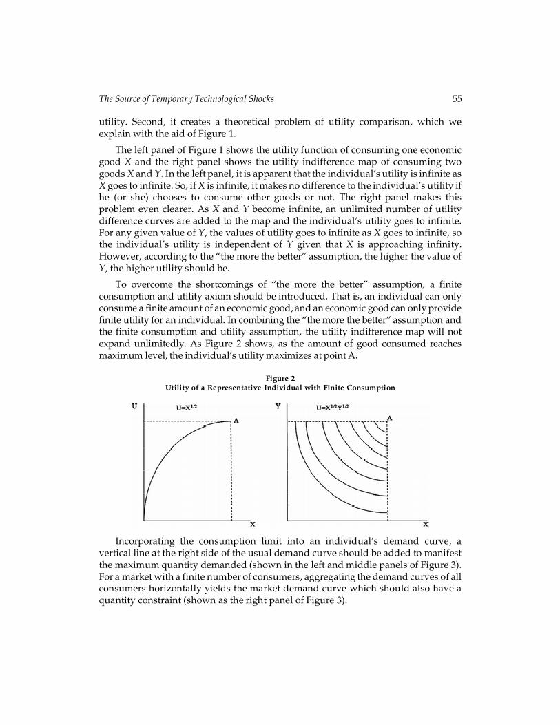
To overcome the shortcomings of “the more the better” assumption, a finiteconsumption and utility axiom should be introduced. That is, an individual can onlyconsume a finite amount of an economic good, and an economic good can only providefinite utility for an individual. In combining the “the more the better” assumption andthe finite consumption and utility assumption, the utility indifference map will notexpand unlimitedly. As Figure 2 shows, as the amount of good consumed reachesmaximum level, the individual’s utility maximizes at point A.

Figure 2Utility of a Representative Individual with Finite Consumption

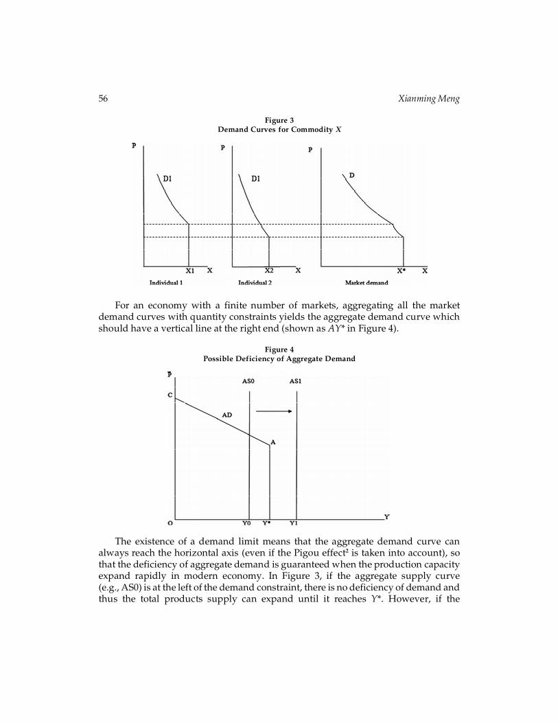
Incorporating the consumption limit into an individual’s demand curve, avertical line at the right side of the usual demand curve should be added to manifestthe maximum quantity demanded (shown in the left and middle panels of Figure 3).For a market with a finite number of consumers, aggregating the demand curves of allconsumers horizontally yields the market demand curve which should also have aquantity constraint (shown as the right panel of Figure 3).

56 Xianming Meng

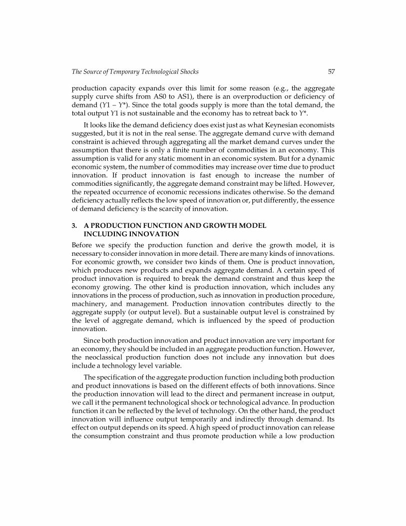
For an economy with a finite number of markets, aggregating all the marketdemand curves with quantity constraints yields the aggregate demand curve whichshould have a vertical line at the right end (shown as AY* in Figure 4).

Figure 3Demand Curves for Commodity X

Figure 4Possible Deficiency of Aggregate Demand

The existence of a demand limit means that the aggregate demand curve canalways reach the horizontal axis (even if the Pigou effect2 is taken into account), sothat the deficiency of aggregate demand is guaranteed when the production capacityexpand rapidly in modern economy. In Figure 3, if the aggregate supply curve(e.g., AS0) is at the left of the demand constraint, there is no deficiency of demand andthus the total products supply can expand until it reaches Y*. However, if the


production capacity expands over this limit for some reason (e.g., the aggregatesupply curve shifts from AS0 to AS1), there is an overproduction or deficiency ofdemand (Y1 – Y*). Since the total goods supply is more than the total demand, thetotal output Y1 is not sustainable and the economy has to retreat back to Y*.

It looks like the demand deficiency does exist just as what Keynesian economistssuggested, but it is not in the real sense. The aggregate demand curve with demandconstraint is achieved through aggregating all the market demand curves under theassumption that there is only a finite number of commodities in an economy. Thisassumption is valid for any static moment in an economic system. But for a dynamiceconomic system, the number of commodities may increase over time due to productinnovation. If product innovation is fast enough to increase the number ofcommodities significantly, the aggregate demand constraint may be lifted. However,the repeated occurrence of economic recessions indicates otherwise. So the demanddeficiency actually reflects the low speed of innovation or, put differently, the essenceof demand deficiency is the scarcity of innovation.

3. A PRODUCTION FUNCTION AND GROWTH MODELINCLUDING INNOVATION

Before we specify the production function and derive the growth model, it isnecessary to consider innovation in more detail. There are many kinds of innovations.For economic growth, we consider two kinds of them. One is product innovation,which produces new products and expands aggregate demand. A certain speed ofproduct innovation is required to break the demand constraint and thus keep theeconomy growing. The other kind is production innovation, which includes anyinnovations in the process of production, such as innovation in production procedure,machinery, and management. Production innovation contributes directly to theaggregate supply (or output level). But a sustainable output level is constrained bythe level of aggregate demand, which is influenced by the speed of productioninnovation.

Since both production innovation and product innovation are very important foran economy, they should be included in an aggregate production function. However,the neoclassical production function does not include any innovation but doesinclude a technology level variable.

The specification of the aggregate production function including both productionand product innovations is based on the different effects of both innovations. Sincethe production innovation will lead to the direct and permanent increase in output,we call it the permanent technological shock or technological advance. In productionfunction it can be reflected by the level of technology. On the other hand, the productinnovation will influence output temporarily and indirectly through demand. Itseffect on output depends on its speed. A high speed of product innovation can releasethe consumption constraint and thus promote production while a low production

58 Xianming Meng

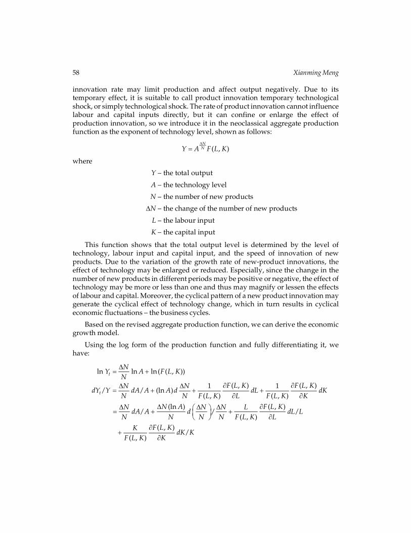
innovation rate may limit production and affect output negatively. Due to itstemporary effect, it is suitable to call product innovation temporary technologicalshock, or simply technological shock. The rate of product innovation cannot influencelabour and capital inputs directly, but it can confine or enlarge the effect ofproduction innovation, so we introduce it in the neoclassical aggregate productionfunction as the exponent of technology level, shown as follows:

( , )N

NY A F L K�

�

where

Y – the total output

A – the technology level

N – the number of new products

�N – the change of the number of new products

L – the labour input

K – the capital input

This function shows that the total output level is determined by the level oftechnology, labour input and capital input, and the speed of innovation of newproducts. Due to the variation of the growth rate of new-product innovations, theeffect of technology may be enlarged or reduced. Especially, since the change in thenumber of new products in different periods may be positive or negative, the effect oftechnology may be more or less than one and thus may magnify or lessen the effectsof labour and capital. Moreover, the cyclical pattern of a new product innovation maygenerate the cyclical effect of technology change, which in turn results in cyclicaleconomic fluctuations – the business cycles.

Based on the revised aggregate production function, we can derive the economicgrowth model.

Using the log form of the production function and fully differentiating it, wehave:

ln ln ln( ( , ))

( , ) ( , )1 1/ / (ln )

( , ) ( , )

(ln ) ( , )/ / /

( , )( , )

/( , )

t

t

NY A F L K

NF L K F L KN N

dY Y dA A A d dL dKN N F L K L F L K K

N A F L KN N N LdA A d dL L

N N N N F L K LF L KK

dK KF L K K

��

� ��

� �

� ��

��


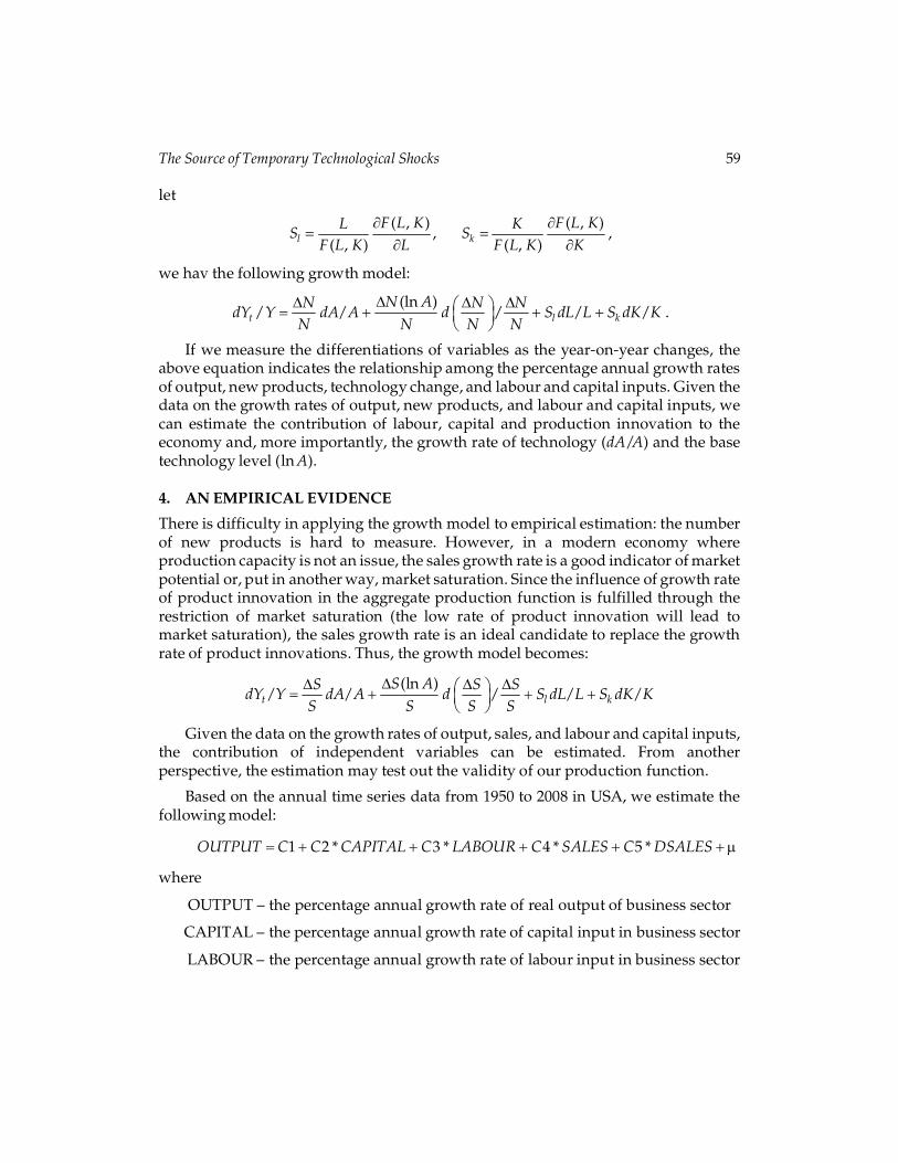
let

( , ) ( , ),

( , ) ( , )l kF L K F L KL K

S SF L K L F L K K

� ��

� �,

we hav the following growth model:

(ln )/ / / / /t l k

N AN N NdY Y dA A d S dL L S dK K

N N N N��

� �.

If we measure the differentiations of variables as the year-on-year changes, theabove equation indicates the relationship among the percentage annual growth ratesof output, new products, technology change, and labour and capital inputs. Given thedata on the growth rates of output, new products, and labour and capital inputs, wecan estimate the contribution of labour, capital and production innovation to theeconomy and, more importantly, the growth rate of technology (dA/A) and the basetechnology level (ln A).

4. AN EMPIRICAL EVIDENCE

There is difficulty in applying the growth model to empirical estimation: the numberof new products is hard to measure. However, in a modern economy whereproduction capacity is not an issue, the sales growth rate is a good indicator of marketpotential or, put in another way, market saturation. Since the influence of growth rateof product innovation in the aggregate production function is fulfilled through therestriction of market saturation (the low rate of product innovation will lead tomarket saturation), the sales growth rate is an ideal candidate to replace the growthrate of product innovations. Thus, the growth model becomes:

(ln )/ / / / /t l k

S AS S SdY Y dA A d S dL L S dK K

S S S S��

� �

Given the data on the growth rates of output, sales, and labour and capital inputs,the contribution of independent variables can be estimated. From anotherperspective, the estimation may test out the validity of our production function.

Based on the annual time series data from 1950 to 2008 in USA, we estimate thefollowing model:

1 2 * 3 * 4 * 5 *OUTPUT C C CAPITAL C LABOUR C SALES C DSALES� � � � � � �

where

OUTPUT – the percentage annual growth rate of real output of business sector

CAPITAL – the percentage annual growth rate of capital input in business sector

LABOUR – the percentage annual growth rate of labour input in business sector

60 Xianming Meng

SALES – the percentage annual growth rate of sales to final demand

DSALES – the percentage annual growth rate of SALES

The time series of growth rates of real output, labour input and capital input arefrom the Net Multifactor Productivity and Cost Table (1948 – 2008) calculated by theBureau of Labour Statistics (BLS)3. The annual growth rates of final sales are from theGDP account provided by the Bureau of Economic Analysis (BEA)4. The E-viewsoftware is used for the model estimation and testing.

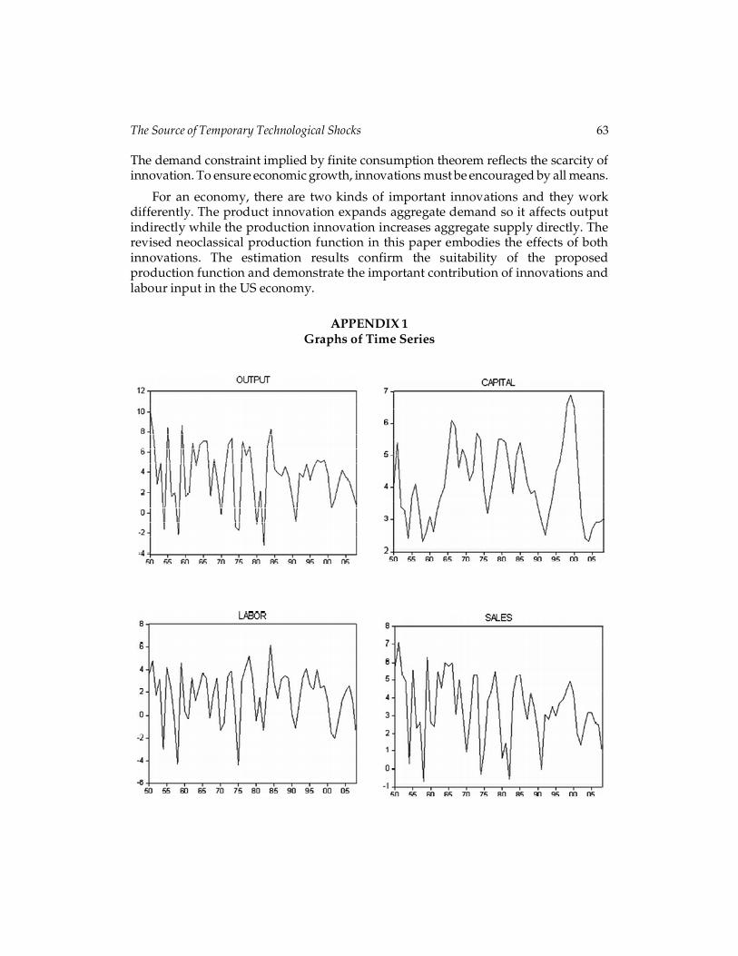
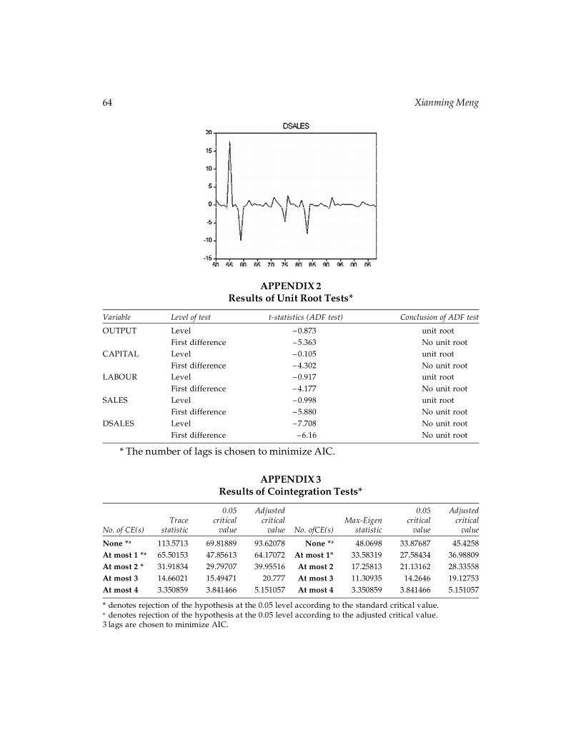
Since most macroeconomic time series data are non-stationary, unit root tests areperformed. Before formal testing procedures are undertaken, the time series data areplotted to allow for visual inspection (see Appendix 1). All time series show notrends, but most of them have intercept, except DSALES. The Augmented Dickey-Fuller (ADF) tests are performed to check the stationarity of all time series. Theresults are listed in Appendix 2. With the exception of DSALES, the PP and ADF testssuggest first order integration for all variables at 5% level of significance. DSALES isfound to be stationary.

Since non-stationary time series are used, the cointegration test has to beperformed. Johansen procedure (see Johansen, 1988; Johansen and Juselius, 1990) isused to test for cointegration among OUTPUT, CAPITAL, LABOUR and SALES. Inimplementing the tests, a deterministic linear trend and incept in the cointegrationequation is included, so that the deterministic trends are removed from thecointegration relationship, and thus the test results are free from the distortion ofdeterministic trends. The trace test suggests 3 cointegration equations while the max-eigenvalue test suggests 2 cointegration equations (see appendix 3).

However, the likelihood ratio (LR) tests in the Johansen procedure is derived fromasymptotic property and the statistic inference may not be applicable to finite sample.Thus, many econometricians express concern about the problem of finite sample size inJohansen’s LR tests for cointegration. Reinsel and Ahn (1988) suggest that a scalingfactor, which is a simple function of T, n, and k (T is the sample size, n is the number ofvariables in the model and k is the number of lags), may be used to obtain finite-samplecritical values from their asymptotic counterparts. Reimers (1992) claims that in finitesamples the Johansen test statistics too often over-rejects the null hypothesis of non-cointegration when it is true and suggests the application of the Reinsel-Ahn method toadjust Johansen’s test statistics by a factor of (T – nk)/T. Cheung and Lai (1993) use thesurface analysis in Monte Carto experiments to estimate the finite-sample criticalvalues for both trace and max-eigen value tests and find that the finite sample bias ofJohansen’s tests is a positive function of T/(T – nk). Following this finding, they claimthat “since both n and k are of positive values, T/(T – nk) is always greater than one forany finite T value, indicating that the tests are biased toward finding cointegration toooften when asymptotic critical values are used. Furthermore, the finite-sample biastoward over-rejection of the no cointegration hypothesis magnifies with increasingvalues of n and k”. (Cheung and Lai, 1993, p. 319).


In the case of this study, the sample size is 60 (T = 59 after adjustment); 5 variablesare included in the model (n = 5); and the AIC indicates the proper lags forcointegration test is 3 (k = 3). So the finite-sample bias in the cointegration test tends tobe large. Following the suggestion of previous studies, T/(T – nk) is used to scale upthe standard critic value. The adjusted critic values are shown in the column next tothe standard critic value in Appendix 3). According to the adjusted critical values, thetrace test suggests two cointegration relationships at 0.05 level while max-eigenvaluetest suggests one cointegration. However, the trace test only marginally suggests thesecond cointegration, so we tend to conclude that there is only one cointegrationamong tested variables.

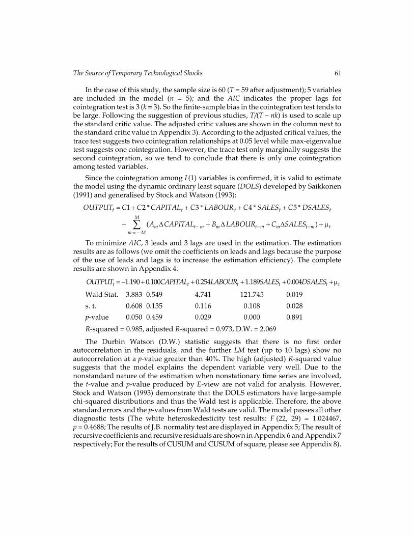
Since the cointegration among I (1) variables is confirmed, it is valid to estimatethe model using the dynamic ordinary least square (DOLS) developed by Saikkonen(1991) and generalised by Stock and Watson (1993):

1 2 * 3 * 4 * 5 *

( )

t t t t tM

m t m m t m m t m tm M

OUTPUT C C CAPITAL C LABOUR C SALES C DSALES

A CAPITAL B LABOUR C SALES� � ��

� � � � �

� � � � � � � ��

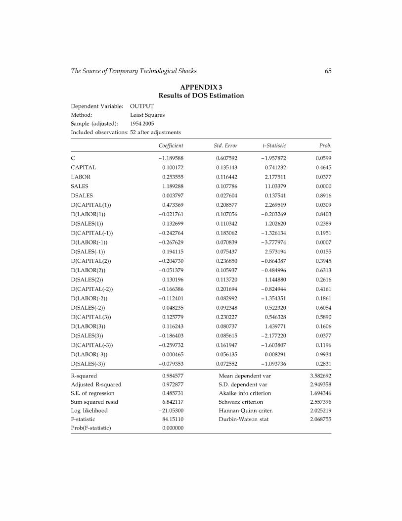
To minimize AIC, 3 leads and 3 lags are used in the estimation. The estimationresults are as follows (we omit the coefficients on leads and lags because the purposeof the use of leads and lags is to increase the estimation efficiency). The completeresults are shown in Appendix 4.

1.190 0.100 0.254 1.189 0.004t t t t t tOUTPUT CAPITAL LABOUR SALES DSALES� � � � � � ��

Wald Stat. 3.883 0.549 4.741 121.745 0.019

s. t. 0.608 0.135 0.116 0.108 0.028

p-value 0.050 0.459 0.029 0.000 0.891

R-squared = 0.985, adjusted R-squared = 0.973, D.W. = 2.069

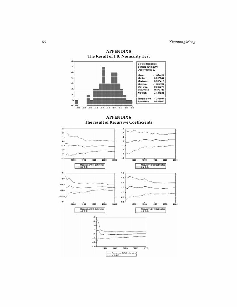
The Durbin Watson (D.W.) statistic suggests that there is no first orderautocorrelation in the residuals, and the further LM test (up to 10 lags) show noautocorrelation at a p-value greater than 40%. The high (adjusted) R-squared valuesuggests that the model explains the dependent variable very well. Due to thenonstandard nature of the estimation when nonstationary time series are involved,the t-value and p-value produced by E-view are not valid for analysis. However,Stock and Watson (1993) demonstrate that the DOLS estimators have large-samplechi-squared distributions and thus the Wald test is applicable. Therefore, the abovestandard errors and the p-values from Wald tests are valid. The model passes all otherdiagnostic tests (The white heteroskedesticity test results: F (22, 29) = 1.024467,p = 0.4688; The results of J.B. normality test are displayed in Appendix 5; The result ofrecursive coefficients and recursive residuals are shown in Appendix 6 and Appendix 7respectively; For the results of CUSUM and CUSUM of square, please see Appendix 8).

62 Xianming Meng

The DOLS estimators reveal the following interesting findings:

First, all independent variables show positive contribution to the output, which isconsistent with the prediction of the aggregate production function.

Second, the growth rate of sales has tremendous positive effects on the growth ofGDP. The large Wald statistic for the coefficient of sales growth rate demonstrates itsimportance. Since the sales growth rates reflect the product innovation rates, thisresults implies the important contribution of production innovation and the necessityto include it in an aggregate production function.

Third, the labour input is significant at around 3% level, but the contribution ofcapital is found insignificant. The greater significance of labour input than capitalinput is consistent with the effect that much more income in the US economy goes tolabour than to capital.

Finally, the insignificance of DSALES is consistent with the theoretic productionfunction. Referring to the production function, the coefficient of DSALES indicatesthe log value of technology level multiplied by the sales growth rate. The log value isquite small; the growth rate of final sales can be positive or negative, and very small invalue (less than 8% as shown in appendix 1). As a result, the average value of the sumof the products should be close to zero as shown by the estimation results.

For contrast and comparison, we also estimated the Solow growth model(omitting the variables SALES and DSALES in the above model and using the samedataset and estimation procedure). The estimation results are:

1.093 0.268 0.809t t t tOUTPUT CAPITAL LABOUR� � � � � �

Wald Stat. 0.565 0.500 6.527

s. t. 1.454 0.379 0.317

p-value 0.452 0.480 0.011

R-squared= 0.818, adjusted R-squared = 0.749, D.W. = 1.277

The (adjusted) R-squared value decreased dramatically and the D.W. statisticsshow the existence of autocorrelation. Both of them indicate the misspecification ofthe model (having omitted important independent variables). The Wald statistics andthe p-values of above estimation also show the significance of labour input and theinsignificance of capital input, but the estimated coefficients for both labour andcapital increase nearly 3 times, which manifests that omission of the innovation(or sales) variable exaggerates the contribution of both labour and capital.

5. CONCLUSION

The preference and utility theory needs modification so as to avoid unlimited utilityand unlimited consumption, which is unrealistic and problematic in a real economy.


The demand constraint implied by finite consumption theorem reflects the scarcity ofinnovation. To ensure economic growth, innovations must be encouraged by all means.

For an economy, there are two kinds of important innovations and they workdifferently. The product innovation expands aggregate demand so it affects outputindirectly while the production innovation increases aggregate supply directly. Therevised neoclassical production function in this paper embodies the effects of bothinnovations. The estimation results confirm the suitability of the proposedproduction function and demonstrate the important contribution of innovations andlabour input in the US economy.

APPENDIX 1Graphs of Time Series

64 Xianming Meng

APPENDIX 2Results of Unit Root Tests*

Variable Level of test t-statistics (ADF test) Conclusion of ADF test

OUTPUT Level – 0.873 unit rootFirst difference – 5.363 No unit root

CAPITAL Level – 0.105 unit rootFirst difference – 4.302 No unit root

LABOUR Level – 0.917 unit rootFirst difference – 4.177 No unit root

SALES Level – 0.998 unit rootFirst difference – 5.880 No unit root

DSALES Level – 7.708 No unit rootFirst difference – 6.16 No unit root

* The number of lags is chosen to minimize AIC.

APPENDIX 3Results of Cointegration Tests*

0.05 Adjusted 0.05 AdjustedTrace critical critical Max-Eigen critical critical

No. of CE(s) statistic value value No. ofCE(s) statistic value value

None *a 113.5713 69.81889 93.62078 None *a 48.0698 33.87687 45.4258At most 1 *a 65.50153 47.85613 64.17072 At most 1* 33.58319 27.58434 36.98809At most 2 * 31.91834 29.79707 39.95516 At most 2 17.25813 21.13162 28.33558At most 3 14.66021 15.49471 20.777 At most 3 11.30935 14.2646 19.12753At most 4 3.350859 3.841466 5.151057 At most 4 3.350859 3.841466 5.151057

* denotes rejection of the hypothesis at the 0.05 level according to the standard critical value.a denotes rejection of the hypothesis at the 0.05 level according to the adjusted critical value.3 lags are chosen to minimize AIC.


APPENDIX 3Results of DOS Estimation

Dependent Variable: OUTPUT

Method: Least Squares

Sample (adjusted): 1954 2005

Included observations: 52 after adjustments

Coefficient Std. Error t-Statistic Prob.

C – 1.189588 0.607592 – 1.957872 0.0599

CAPITAL 0.100172 0.135143 0.741232 0.4645

LABOR 0.253555 0.116442 2.177511 0.0377

SALES 1.189288 0.107786 11.03379 0.0000

DSALES 0.003797 0.027604 0.137541 0.8916

D(CAPITAL(1)) 0.473369 0.208577 2.269519 0.0309

D(LABOR(1)) – 0.021761 0.107056 – 0.203269 0.8403

D(SALES(1)) 0.132699 0.110342 1.202620 0.2389

D(CAPITAL(-1)) – 0.242764 0.183062 – 1.326134 0.1951

D(LABOR(-1)) – 0.267629 0.070839 – 3.777974 0.0007

D(SALES(-1)) 0.194115 0.075437 2.573194 0.0155

D(CAPITAL(2)) – 0.204730 0.236850 – 0.864387 0.3945

D(LABOR(2)) – 0.051379 0.105937 – 0.484996 0.6313

D(SALES(2)) 0.130196 0.113720 1.144880 0.2616

D(CAPITAL(-2)) – 0.166386 0.201694 – 0.824944 0.4161

D(LABOR(-2)) – 0.112401 0.082992 – 1.354351 0.1861

D(SALES(-2)) 0.048235 0.092348 0.522320 0.6054

D(CAPITAL(3)) 0.125779 0.230227 0.546328 0.5890

D(LABOR(3)) 0.116243 0.080737 1.439771 0.1606

D(SALES(3)) – 0.186403 0.085615 – 2.177220 0.0377

D(CAPITAL(-3)) – 0.259732 0.161947 – 1.603807 0.1196

D(LABOR(-3)) – 0.000465 0.056135 – 0.008291 0.9934

D(SALES(-3)) – 0.079353 0.072552 – 1.093736 0.2831

R-squared 0.984577 Mean dependent var 3.582692

Adjusted R-squared 0.972877 S.D. dependent var 2.949358

S.E. of regression 0.485731 Akaike info criterion 1.694346

Sum squared resid 6.842117 Schwarz criterion 2.557396

Log likelihood – 21.05300 Hannan-Quinn criter. 2.025219

F-statistic 84.15110 Durbin-Watson stat 2.068755

Prob(F-statistic) 0.000000

66 Xianming Meng

APPENDIX 5The Result of J.B. Normality Test

APPENDIX 6The result of Recursive Coefficients


APPENDIX 8The Result of CUSUM and CUSUM of Square

APPENDIX 7The Result of Recursive Residuals

NOTES

1. For the further development of the real business cycle model please also see Prescott(1986) and Plosser (1989)

2. For Pigou effect please see Pigou (1943).3. These data are available from BLS website. http://www.bls.gov/mfp/mprdload.htm, Historical

multifactor productivity measures (SIC 1948-87 linked to NAICS 1987-2008)

68 Xianming Meng

4. The data are a vailable from BEA website. http://www.bea.gov/national/nipaweb/SelectTable.asp?Selected=Y, Table 1.4.1. Percent Change From Preceding Period in Real Gross DomesticProduct, Real Gross Domestic Purchases, and Real Final Sales to Domestic Purchasers.

REFERENCES

Cheung Y-W., and Lai K. S., (1993), Finite-Sample Sizes of Johansen’s Likelihood Ratio Testsfor Cointegration, Oxford Bulletin of Economics and Statistics, Vol. 55, pp. 313-328.

Johansen S., (1988), Statistical Analysis of Cointegration Vectors, Journal of Economic Dynamicsand Control, Vol. 12, pp. 231-254.

Johansen S., and Jueslius K., (1990), Maximum Likelihood Estimation and Inference onCointegration – With Applications to the Demand for Money, Oxford Bulletin of Economicsand Statistics, Vol. 52, pp. 169-210.

Kydland F. E., and Prescott E. C., (1982), Time to Build and Aggregate Fluctuations,Econometrica, Vol. 51, pp. 1345-1370.

Mankew N. G., (1989), Real Business Cycles: A New Keynesian Perspective, Journal of EconomicPerspectives, Summer.

Pigou A. C., (1943), The Classical Stationary State, Economic Journal, (December), pp. 343-351.Plosser C. I., (1989), Understanding Real Business Cycles, Journal of Economic Perspectives,

Summer.Prescott E. C., (1986), Theory Ahead of Business Cycle Measurement, Federal Reserve Bank of

Minneapolis Quarterly Review, Fall.Reimers H-E., (1992), Comparisons of Tests for Multivariate Cointegration, Statistical Papers,

Vol. 33, pp. 335-359.Saikkonen P., (1991), Asymptotically Efficient Estimation of Cointegration Regressions,

Econometric Theory, Vol. 7, pp. 1-21.Stock J. H., and Watson M. W., (1993), A Simple Estimator of Cointegrating Vectors in Higher

Order Integrated Systems, Econometrica, Vol. 61, pp. 783-820.

Documents

THE SOURCE OF TEMPORARY TECHNOLOGICAL …serialsjournals.com/serialjournalmanager/pdf/1345112660.pdftechnological changes contradicts our basic ... sources of temporary and permanent