The slow convergence of per capita income between the ...between the developing countries: “growth resistance” and sometimes “growth tragedy” Gilles Dufrénot, Valérie Mignon

1

_____________________________________________________________________ CREDIT Research Paper

No. 09/03 _____________________________________________________________________

The slow convergence of per capita income between the developing countries:

“growth resistance” and sometimes “growth tragedy”

Gilles Dufrénot, Valérie Mignon and Théo Naccache Abstract This paper provides empirical evidence that there is no absolute convergence between the GDP per capita of the developing countries since 1950. Relying upon recent econometric methodologies (non-stationary long-memory models, wavelet models and time-varying factor representation models), we show that the transition paths to long-run growth are very persistent over time and non-stationary, thereby yielding a variety of potential growth steady states (conditional convergence). Our findings do not support the idea according to which the developing countries share a common factor (such as technology) that eliminates growth divergence in the very long run. Instead, we conclude that growth is an idiosyncratic phenomenon that yields different forms of transitional economic performance: growth tragedy (some countries with an initial low level of per capita income diverge from the richest ones), growth resistance (with many countries experiencing a low speed of growth convergence), and rapid convergence. JEL Classification: C32; E10; 041. Keywords: growth convergence, developing countries, long memory, wavelets, time-varying factor models. _____________________________________________________________________ Centre for Research in Economic Development and International Trade, University of Nottingham

2

_____________________________________________________________________ CREDIT Research Paper

No. 09/03

The slow convergence of per capita income between the developing countries: “growth resistance” and sometimes

“growth tragedy”

by

Gilles Dufrénot, Valérie Mignon and Théo Naccache

Outline 1. Introduction 2. Brief review of growth convergence testing and new methodologies 3. Growth convergence and fractional integration 4. Modelling the slowly varying transition paths to long-run growth 5. Conclusion The Authors

Gilles Dufrénot, Professor of International Economics, DEFI (University of Aix-Marseille 2) and CEPII (Paris), France. Email: [email protected]. Valérie Mignon, Professor of Economics, EconomiX-CNRS, University of Paris Ouest and CEPII, (Paris), France. Email: [email protected]. Théo Naccache, EconomiX-CNRS, University of Paris Ouest, Paris, France. Email: [email protected].

_____________________________________________________________________ Research Papers at www.nottingham.ac.uk/economics/credit/

3

1. Introduction

Many empirical studies fail to find support of income convergence among the developing countries. Only a few of them have grown faster than the others, namely the so-called emerging economies (Brazil, China, India, Mexico, South-East Asian countries, oil-exporting countries in the Middle East, Central and Eastern European countries). The most striking example of the widening gap is Africa. Examining whether there could be new emerging economies in Africa by 2020, Berthélémy and Soderling (2001) concluded that “even if one makes relatively optimistic assumptions, Africa is not likely to reach Asian tigers levels of growth”. To explain this income inequality, a growing literature has been focusing since the 2000’s on the interaction between structural factors and the process of economic development. Several authors suggest that income inequality among the developing nations reflects distributional cross-section heterogeneity, in the sense that economies are unequally endowed in terms of institutional, political, geographical, cultural and historical environments.1 These inequalities can induce divergent growth performances, if these factors impede the technological creation.

In this paper, we shall not discuss the validity of the “institutional” approach of economic growth to explain the huge income inequality across the developing countries. We focus on one consequence of such explanations, namely the slow convergence to growth and the non-stationary dynamics inherent to the transition paths. Indeed, if the economic factors interact with a large number of negative structural features, then some countries may face a phenomenon of “growth resistance” implying a very long transition dynamics towards the richest countries’ incomes. Furthermore, if over time, the negative influence of the non-economic structural factors acts faster than the positive effects of technology creation, human being, saving, etc., then it is possible that no recovery or catching-up dynamics will be observed and that some diverging growth paths may be manifest. We call this situation a “growth tragedy”, or to paraphrase Easterly (2002), “an elusive quest for growth”. An optimistic view would suggest that, even if the speeds of convergence are slow, an ultimate convergence to the richest countries’ income level can be achieved. This is the message of the Solow (1956)’s growth model and of Lucas (2002) who theoretically explain why income inequality can be considered as an historical transient. A pessimistic view would stress that the growth strategies that are good for the emerging economies do not suit the situation of the poorest nations. This view is supported by Easterly (2002) or Stiglitz (2002), and Easterly (2003) documents what he calls a “growth puzzle”, showing that during the eighties and the nineties, many poor developing nations stagnated in spite of the adoption of policy reforms based on the standard theoretical models of economic growth.

Whether the differentials of growth performance between the developing countries are mean-reverting—and hence indicative of long-run convergence—or whether they are believed to become drastically different in the future is still a hotly debated issue in the circles of policymakers. A key question is whether the empirical evidence would point to a narrowing of the cross-countries’ differentials through time, despite the long transient dynamics, or 1 See for instance the collection of papers in the Journal of Monetary Economics (2003), and recent papers by Banerjee and Somanathan (2007) and Huillery (2009).

4

whether the developing world cannot be considered as integrated at all, even in the very far future. Viewed from the first standpoint, there is space for policies aiming at accelerating the countries’ growth dynamics (policies that break growth resistance, for instance through a faster speed of learning technology, an improvement in governance, the adoption of cultural and social schemes that are pro-growth). From the second standpoint, the sharply differing growth evolutions would be an unsolved puzzle for the researchers. Both views are shared today by the economists. On one hand, the idea of an African tragedy is debated since the nineties, and economists provide various explanations supporting the view that the continent is in a poverty trap and has few capacities to take-off (see, among others, Kabou (1991), Bairoch (1993), and the special issue of the journal Philosophy and Development (2004)). On the other hand, some developing countries, specifically in Asia, have grown rapidly by experiencing in 50 years a growth dynamics that the industrialized countries had taken 150 years to reach. In this case, if we observe a slow convergence between them, this simply reflects conditional convergence in the sense that the countries are undergoing economic development processes that are idiosyncratic. In these countries, policymakers may be inclined to promote their own model of development (for instance, economists talk about “a Chinese model”).

This paper provides empirical evidence that the transition paths to long-run growth in the developing countries are very persistent over time and non-stationary, thereby yielding a variety of potential growth steady states (conditional convergence). The slow and non-stationary dynamics are illustrative of complex transition paths to growth: divergence can manifest sometimes, followed by catching-up dynamics, feedback to divergence and then convergence. Our findings do not support the idea according to which the developing countries share a common factor that eliminates growth divergence in the very long run. Instead, we conclude that growth is an idiosyncratic phenomenon that yields different forms of transitional economic performance: growth tragedy (some countries with an initial low level of per capita income diverge from the richest ones), growth resistance (with many countries experiencing a low speed of growth convergence), and fast convergence. These results are obtained by applying recent techniques proposed in the econometric literature: non-stationary long-memory models, wavelet models and time-varying factor representation models.

The rest of the paper is organized as follows. Section 2 provides a brief review of the empirical testing of growth convergence and specifies what is new with the techniques that are used in the paper. In Section 3, we provide evidence that growth convergence is persistent and non-stationary over time in the developing countries. In Section 4, this finding is interpreted in terms of slowly varying transition paths. Finally, Section 5 concludes.

2. Brief review of growth convergence testing and new methodologies

There is a huge literature concerned with the empirical testing of the conditional convergence of per capita GDPs across countries. During the eighties, the techniques employed involved testing whether poor countries tended to grow faster than the rich ones using β-convergence

5

models. β-convergence is defined by a negative correlation between the growth rate of per capita income and the initial income level. This convergence is usually conditional because countries have different structural characteristics (propensity to save, population growth rate, technological progress, etc.). A variety of estimates based on the β-convergence model have been proposed using both time series and panel data methods, and many contributions conclude in favor of the hypothesis of a catching-up effect (or conditional convergence) between the poor and rich countries. Conversely, absolute convergence—with the poorest countries reaching the richest countries’ per capita income—is rare.2

The nineties also marked an intensive activity in the empirics of growth convergence through studies applying unit root and cointegration methods (using both time series and panel data). Convergence is tested by applying unit root tests to the differences between GDP per capita series of two countries, or by considering cointegrating vectors in systems composed of GDP per capita series of two or more countries. This approach allows a distinction between long-run convergence (cointegration with an identical common stochastic trend) and catching-up convergence (cointegration with the stochastic trend of one country being proportional to that of the benchmark country).3 Lau (1999) provides a theoretical justification to the use of cointegration techniques, showing that integration and cointegration properties arise intrinsically in stochastic endogenous growth models and produce steady-state growth even in the absence of exogenous growth-generating mechanisms. However, when one uses the usual I(0)/I(1) approach or the standard cointegration framework, evidence in favor of convergence or catching-up effects is infrequently found, notably among the developing countries. A recent strand of the literature puts the blame of this failure to find convergence on spurious regressions. Indeed, if the GDP per capita series were neither I(1) nor I(0), but fractionally integrated, then the usual non-stationary and non-cointegration tests would spuriously reject or accept the convergence hypothesis.

Recent research claims that growth convergence cannot be appropriately examined in a I(0)/I(1) setting given the evidence in the empirical literature that aggregate outputs are suitably modeled by fractionally integrated processes. Such processes are designed to account for the long-memory characteristic of the series through a differencing parameter d that can take fractional values and not only integer ones.4 Accordingly, empirical studies of growth convergence have turned to new methodologies based on fractional integration setting 2 Examples of papers are those of Baumol (1986), Bradford DeLong (1988), Barro (1991), Barro and Sala-i-Martin (1992, 1995), Mankiw, Romer and Weil (1992), Verspagen (1995), Islam (1995), Lee, Pesaran and Smith (1998), Bond, Hoeffler and Temple (2001), Tsangarides (2001), Hoeffler (2002), Lee and McAleer (2004). 3 See Carlino and Mills (1993), Bernard and Durlauf (1995, 1996), Ben-David (1996), Evans (1996), Li and Papell (1999), Cellini and Scorcu (2000), Strauss (2000), Holmes (2000), Fleissig and Strauss (2001), Ericsson and Halket (2002), Cheung and Pascual (2004). 4Various explanations are related to the existence of long-memory components in aggregate output and the fractional integration hypothesis for GDP data. The justifications rely on the fact that fractional integration is a consequence of aggregation over heterogeneous firms (Abadir and Talmain (2002)), multiple sectors (Haubrich and Lo (2001)) or cross-sectional heterogeneity in a Solow-Swan growth model (Michelacci and Zaffaroni (2000)). The fractional integration hypothesis has been investigated in several empirical papers. Some authors show that, over the past, spurious breaks have been mistaken for fractional integration in GDP series (Hsu (2001), Krämer and Sibbertsen (2002)). Others find that the aggregate output is well modeled by long-memory processes à la Granger-Joyeux (Diebold and Rudebusch (1989), Halket (2005), Mayoral (2006)) and characterized by seasonal long memory (Gil-Alana (2001)).

6

(Michelacci and Zaffaroni (2000), Beyaert (2004), Halket (2005), Cunado, Gil-Alana and Perez de Gracia (2006)). Meanwhile, such studies remain few in the literature and essentially concern the developed countries. To our knowledge, there exists no empirical investigation so forth relating to the developing countries, though the question of real convergence of the poorest countries has recently known a renewal interest in the public debate.

In this paper, we fill this gap by applying some robust fractional integration based tests to the group of the developing countries. There are some differences in comparison with the methodologies usually employed that we need to highlight. When researchers estimate the long-memory parameter of an ARFIMA5 model (say d), a widespread approach is to restrict the interval of this parameter to the range (-0.5, 0.5). Indeed, in this interval, a fractionally integrated process is invertible and stationary. Doing this, however leads to two major caveats, as far as we analyze the convergence of per capita income in a group of countries. Firstly, we eliminate a number of convergence situations by not considering the case for which the fractional integration parameter d varies between 0.5 and 1 (mean-reverting dynamics). Secondly, we also do not consider situations of divergence (d>1). Restricting to the interval (-0.5, 0.5) can lead to a misleading rejection of the convergence hypothesis if the estimated d is above 0.5. Another widespread practice is to test for the presence of a stochastic and/or deterministic trend in the series as a first step (these trends are helpful to discriminate between absolute and conditional convergence). If such components are found, then the raw series are transformed before the estimation of the long-memory parameter (either by considering the first-difference or by subtracting the deterministic trend). Meanwhile, these preliminary transformations affect the components of the original data. Indeed, if a time series is not I(1), but I(d) with d fractional and below 1, these transformations may induce an over-differentiation, thereby introducing fictive dynamic structure in the series. In this case, one obtains a biased estimation of d (Agiakloglou, Newbold and Wohar (1993), Hurvich and Ray (1995)). Further, the ordinary least square estimate of the trend coefficients when the errors are I(d) is not efficient (see Sun, Phillips and Lee (1999)). This implies that, by detrending the series as is usually done, one does not appropriately remove the trend components in the raw data.

To overcome these caveats, we make use of fractional integration tests that are robust to the deterministic trend, stochastic trend and explosive components (d>1) in the data. We consider generalizations of Geweke and Porter-Hudak (GPH, 1983) and Whittle estimators to the case of non-stationary long-memory models as proposed by Velasco (1999), Kim and Phillips (2006) and Shimotsu and Phillips (2000, 2005, 2006). The methodologies are based on a modified version of the log-periodogram equation. We investigate the convergence of GDP per capita data for the developing countries belonging to different continents (Africa, Central and Latin America, Asia and Middle East) as well as for subgroups of countries over the period from 1950 to 2006 using the updated Madison (2008)’s database. Applying the techniques described above, we find strong evidence of very slow convergence dynamics to 5 Auto Regressive Fractionally Integrated Moving Average. ARFIMA processes were introduced by Granger and Joyeux (1980) and Hosking (1981). They are characterized by a fractional differencing parameter d which accounts for the long-term dynamics, while traditional AR and MA components capture the short-term dynamics of the series.

7

long-run growth and of conditional, rather than absolute, convergence. Such a finding is in accordance with the idea of a growth resistance phenomenon.

Another recent area of research in the growth convergence literature focuses on transient divergence behavior. The idea, suggested by Phillips and Sul (2007a, 2007b), amounts to say that countries around the world share common underlying factors (technology, culture, areas of economic integration, etc.) that act as “attractors”, thereby implying that poor and rich countries ultimately necessarily converge towards each other. Their approach can be seen as a renewal of the concept of “clubs of convergence”. Initial income differences narrowed over time because the divergent dynamics implied by the idiosyncratic factors of growth are progressively dominated by the common components in economic growth. However the diffusion progress is not temporally uniform and one can observe a variety of transition schemes with periods of divergence, catching-up and convergence that alternate over time. So the convergence process is non-stationary. In this paper, we use this body of the literature to explain our finding of non-stationary long-memory model by the presence of slowly and non-monotonic time-varying transition paths. We conclude that the developing countries do not share common factors driving their income to the same level in the long run. The similar transition paths assumption is evidently rejected and several alternative situations can arise: conditional convergence, but also divergence as reflected for instance by growth tragedy (countries with initial low income per capita that stay behind the others with negative growth rates).

3. Growth convergence and fractional integration

3.1. The framework

The use of fractional integration techniques to study growth convergence can be done in two manners. One way is to use an economic model as a benchmark analytical framework. For instance, Michelacci and Zaffaroni (2000) introduce fractional integration in a Solow-Swan growth model by assuming cross-sectional heterogeneity in the speed with which different firms in the same country adjust their production. They show that the usual 2% rate of convergence found in the literature is the outcome of an underlying fractional integration parameter strictly between 0.5 and 1. Another possibility is to use a model-free approach. Although the latter may be subject to the criticism of “measurement without theory”, it has become current wisdom in the empirical literature on growth convergence. Within a fractional integration setting, definitions of convergence are provided along the following lines.

Let itY and j

tY be the log of the output per capita of country i and j respectively at time t (t = 1,…,T). The output differential is described by the following equation:

jiNiI(d)XXtYY ttj

ti

tyt ≠=++=−=Λ ,,...,1 ,~ ,βα (1)

8

The output differential is defined as a deterministic trend plus a fractional noise component (Xt). The latter is a long-memory process both in the covariance and spectral density sense.6 Specifically, the process Xt is governed by the following equation:

( ) ( )2,0~ ,)(1 εσεε iidLCXL tttd =− (2)

where L is the lag operator, ∑∞

=

=0

,)(k

kk LcLC C(0) = I, and d is the fractional integration

parameter. We assume that the process is invertible ( 5.0−>d ). In this case, Xt can be rewritten as an infinite AR(p) process:

( )( ) ( ) ( )d

kdkddkdLCXd

d

kkk

tktk −Γ=

+Γ−Γ−Γ

==+−

∞→

∞

=−∑

)1(

k0

)(lim ,1

)( ,)()( ππεπ (3)

where Γ is the Gamma function. The properties of a process like (2) have been extensively studied in the literature when ( )5.0,5.0−∈d , that is when it is invertible and stationary and

0≠d .7 Its autocovariance coefficients decay towards zero smoothly (at a hyperbolic rate) and its spectral density diverges to infinity as frequencies tend to zero. In this paper, we only impose the invertibility condition, that is the restriction 5.0−>d .

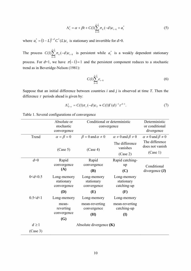
Different definitions of convergence and divergence can be stated depending upon the values of d, α and β.

Case 1. Deterministic divergence ( )0 and 0 ≠≠ βα . This happens when the parameters α and β are such that the initial GDP per capita difference gets bigger over time. Suppose that

0>α . Then, if β > 0, any initial difference between countries i and j is magnified over time

and the countries diverge in a deterministic way.

Case 2. Catching-up dynamics ( )0 and 0 ≠≠ βα . This occurs when the parameters α and β take values that push any initial difference to zero over time (for instance when the deterministic trend has a significant negative slope). Catching-up effects may manifest in several manners:

• Case 2.1. 05.0 ≤<− d . Xt is short-memory, that is I(0).8 The coefficients πk in (3) reduce to (1/k) and decay rapidly towards zero. This case corresponds to a situation of “catching-up convergence” as defined by Bernard and Durlauf (1996). In the context of fractional integration, this configuration can be qualified as “rapid catching-up” or “short-memory catching-up”.

• Case 2.2. 5.00 << d . Xt is a long-memory stationary process. The autoregressive coefficients in (3) decay smoothly, meaning that any difference observed in the output in the remote past still has an influence in the current year. This situation is referred to

6 See Parzen (1981). 7 See Granger and Joyeux (1980) and Hosking (1981). 8 This case includes anti-persistence.

9

as long-memory catching-up. This occurs for instance when a country spends a long time on the transition path towards the common long-run deterministic trend.

• Case 2.3. 15.0 << d . Xt is a long-memory non-stationary, but mean-reverting process. The autoregressive coefficients in (3) are characterized by a high persistence, meaning that any difference observed in the output in the very far past has a long-lasting influence. This situation is referred to as long-memory mean-reverting catching-up.

Case 3. 1≥d . Xt is explosive. In this situation, there is a magnification effect. Any initial difference is not expected to be reversed in the future. This is “stochastic divergence”.

Case 4. Deterministic convergence or conditional convergence ( )0 and 0 ≠= αβ . Depending upon the value of d, the following three cases of convergence can be distinguished:

• Case 4.1. 05.0 ≤<− d . This case corresponds to strict conditional convergence and has been examined by Li and Papell (1999).

• Case 4.2. 5.00 << d . This case refers to long-memory conditional convergence.

• Case 4.3. 15.0 << d . This corresponds to long-memory mean-reverting convergence.

Case 5. Absolute or stochastic convergence ( )0== βα . Absolute or unconditional convergence may be zero-mean convergence in Bernard and Durlauf (1996)’s sense (d=0), long-memory stochastic convergence ( 5.00 << d ) or long-memory mean-reverting convergence ( 15.0 << d ).

The different types of convergence and divergence are summarized in Table 1. Compared with the I(0)/I(1) approach of convergence, the above definitions entail several novelties. Firstly, by allowing for fractional integration, they permit to separately identify two kinds of convergence, namely stationary convergence and mean-reverting convergence. Such a distinction is important because it implies that absolute and conditional convergences can be non-stationary (in Section 4 we study one implication of such a property). Secondly, the fractional integration approach allows intermediate cases between the two configurations that are common wisdom in the literature (on one side the fact that initial differences between countries are perfectly remembered in the future, on the other side the fact that initial differences decay exponentially fast). In practice, the differences can be more or less persistent, so that there exists a continuum of situations between the I(0) and I(1) cases. To see this, Equations (1) and (2) can be re-written using the trend-cycle decomposition methodology initially proposed by Beveridge and Nelson (1981). Following Johansen (1995), C(L) in (2) can be written as:

( ) . ,)( ),(1)1()(1

*

0

*** ∑∑∞

+=

∞

=

−==−+=jk

kjj

jj ccLcLCLCLCLC (4)

So, Equation (1) is now expressed as follows:

10

∑−

=− +−++=Λ

1

0

*)()1(t

ktktk

yt adCt επβα (5)

where ( ) td

t LCLa ε)(1 *1* −−= is stationary and invertible for d>0.

The process ∑−

=−−

1

0)()1(

t

kktk dC επ is persistent while *

ta is a weakly dependent stationary

process. For d=1, we have ( ) 11 =−π and the persistent component reduces to a stochastic trend as in Beveridge-Nelson (1981):

∑−

=−

1

0)1(

t

kktC ε (6)

Suppose that an initial difference between countries i and j is observed at time T. Then the difference τ periods ahead is given by:

.)()1()()1( 11 −−+ Γ≈−=Λ d

TyT dCdC τεπττ (7)

Table 1. Several configurations of convergence

Absolute or stochastic

convergence

Conditional or deterministic convergence

Deterministic or conditional

divergence Trend 0== βα

(Case 5)

0 and 0 ≠= αβ

(Case 4)

0 and 0 ≠≠ βα

The difference vanishes (Case 2)

0 and 0 ≠≠ βαThe difference does not vanish

(Case 1)

d=0 Rapid convergence

(A)

Rapid convergence

(B)

Rapid catching-up (C)

Conditional

divergence (J) 0<d<0.5 Long-memory

stationary convergence

(D)

Long-memory stationary

convergence (E)

Long-memory stationary

catching-up (F)

0.5<d<1 Long-memory mean-

reverting convergence

(G)

Long-memory mean-reverting

convergence (H)

Long-memory mean-reverting

catching-up (I)

1≥d (Case 3)

Absolute divergence (K)

11

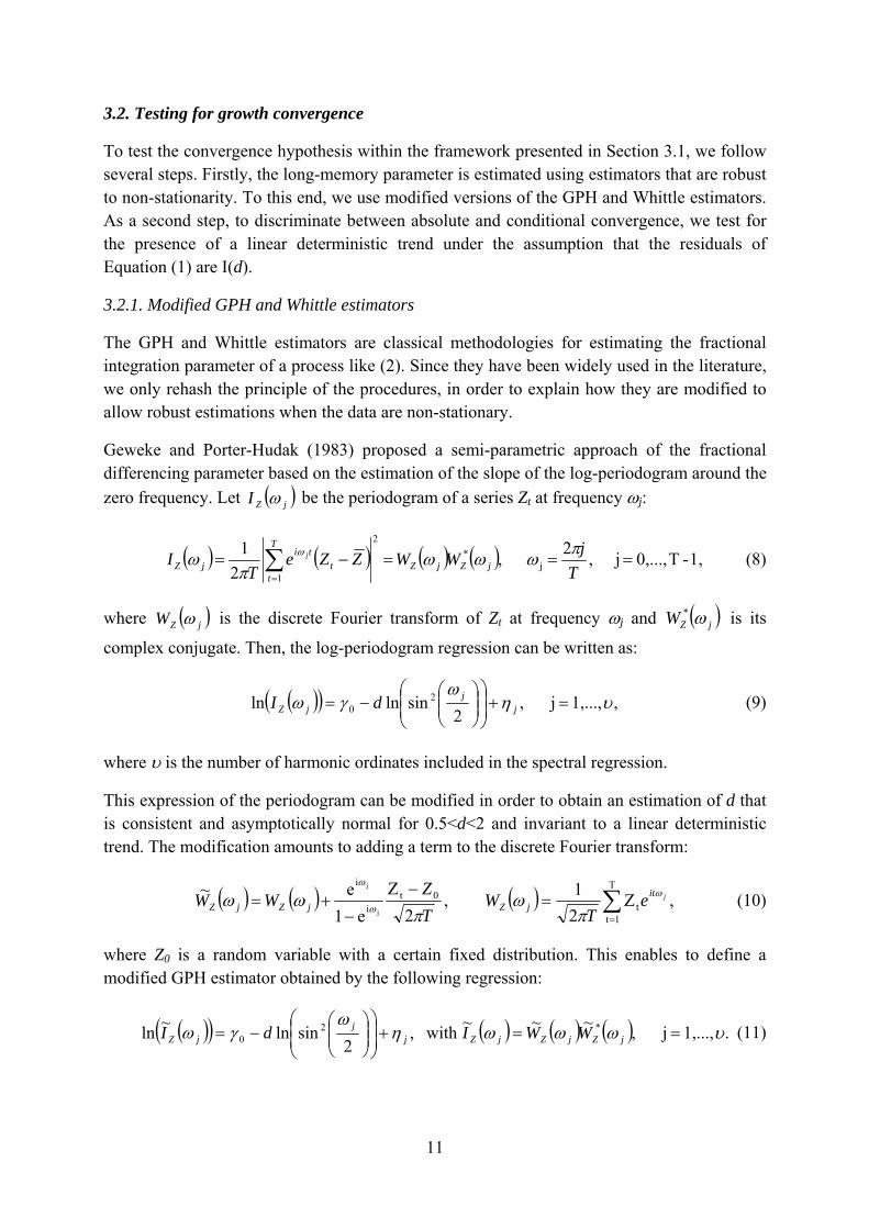
3.2. Testing for growth convergence

To test the convergence hypothesis within the framework presented in Section 3.1, we follow several steps. Firstly, the long-memory parameter is estimated using estimators that are robust to non-stationarity. To this end, we use modified versions of the GPH and Whittle estimators. As a second step, to discriminate between absolute and conditional convergence, we test for the presence of a linear deterministic trend under the assumption that the residuals of Equation (1) are I(d).

3.2.1. Modified GPH and Whittle estimators

The GPH and Whittle estimators are classical methodologies for estimating the fractional integration parameter of a process like (2). Since they have been widely used in the literature, we only rehash the principle of the procedures, in order to explain how they are modified to allow robust estimations when the data are non-stationary.

Geweke and Porter-Hudak (1983) proposed a semi-parametric approach of the fractional differencing parameter based on the estimation of the slope of the log-periodogram around the zero frequency. Let ( )jZI ω be the periodogram of a series Zt at frequency ωj:

( ) ( ) ( ) ( ) 1,-T0,...,j ,2 ,2

1j

*2

1===−= ∑

= TjWWZZe

TI jZjZ

T

tt

tijZ

j πωωωπ

ω ω (8)

where ( )jZW ω is the discrete Fourier transform of Zt at frequency ωj and ( )jZW ω* is its

complex conjugate. Then, the log-periodogram regression can be written as:

( )( ) ,1,...,j ,2

sinlnln 20 υη

ωγω =+⎟

⎟⎠

⎞⎜⎜⎝

⎛⎟⎟⎠

⎞⎜⎜⎝

⎛−= j

jjZ dI (9)

where υ is the number of harmonic ordinates included in the spectral regression.

This expression of the periodogram can be modified in order to obtain an estimation of d that is consistent and asymptotically normal for 0.5<d<2 and invariant to a linear deterministic trend. The modification amounts to adding a term to the discrete Fourier transform:

( ) ( ) ( ) ,Z21 ,

2Z

e1e~ T

1tt

0ti

i

j

j

∑=

=−

−+= jit

jZjZjZ eT

WTZ

WW ωω

ω

πω

πωω (10)

where Z0 is a random variable with a certain fixed distribution. This enables to define a modified GPH estimator obtained by the following regression:

( )( ) ( ) ( ) ( ) .1,...,j ,~~~ with ,2

sinln~ln *20 υωωωη

ωγω ==+⎟

⎟⎠

⎞⎜⎜⎝

⎛⎟⎟⎠

⎞⎜⎜⎝

⎛−= jZjZjZj

jjZ WWIdI (11)

12

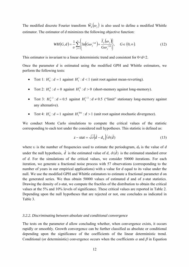
The modified discrete Fourier transform ( )jZW ω~ is also used to define a modified Whittle

estimator. The estimator of d minimizes the following objective function:

( ) ( ) ( ) ( ).,0 ,~

ln1,1

22 ∞∈

⎪⎭

⎪⎬⎫

⎪⎩

⎪⎨⎧

+= ∑=

−− G

GI

GdGWHj

dj

jZdj

υ

ωω

ωυ

(12)

This estimator is invariant to a linear deterministic trend and consistent for 0<d<2.

Once the parameter d is estimated using the modified GPH and Whittle estimators, we perform the following tests:

• Test 1: 1:10 =dH against 1:1

1 <dH (unit root against mean-reverting).


1 >dH (short-memory against long-memory).

• Test 3: 5.0:2/10 =dH against 5.0:2/1

1 ≠dH (“limit” stationary long-memory against any alternative).


1 >dH bis (unit root against stochastic divergence).

We conduct Monte Carlo simulations to compute the critical values of the statistic corresponding to each test under the considered null hypotheses. This statistic is defined as:

( ) )ˆ(ˆˆ0 dddstatz συ −=− (13)

where υ is the number of frequencies used to estimate the periodogram, d0 is the value of d under the null hypothesis, d̂ is the estimated value of d, )ˆ(ˆ dσ is the estimated standard error of d. For the simulations of the critical values, we consider 50000 iterations. For each iteration, we generate a fractional noise process with 57 observations (corresponding to the number of years in our empirical applications) with a value for d equal to its value under the null. We use the modified GPH and Whittle estimators to estimate a fractional parameter d on the generated series. We thus obtain 50000 values of estimated d and of z-stat statistics. Drawing the density of z-stat, we compute the fractiles of the distribution to obtain the critical values at the 5% and 10% levels of significance. These critical values are reported in Table 2. Depending upon the null hypotheses that are rejected or not, one concludes as indicated in Table 3.

3.2.2. Discriminating between absolute and conditional convergence

The tests on the parameter d allow concluding whether, when convergence exists, it occurs rapidly or smoothly. Growth convergence can be further classified as absolute or conditional depending upon the significance of the coefficients of the linear deterministic trend. Conditional (or deterministic) convergence occurs when the coefficients α and β in Equation

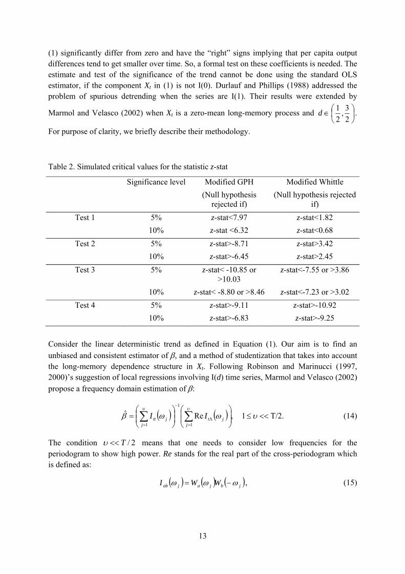
13

(1) significantly differ from zero and have the “right” signs implying that per capita output differences tend to get smaller over time. So, a formal test on these coefficients is needed. The estimate and test of the significance of the trend cannot be done using the standard OLS estimator, if the component Xt in (1) is not I(0). Durlauf and Phillips (1988) addressed the problem of spurious detrending when the series are I(1). Their results were extended by

Marmol and Velasco (2002) when Xt is a zero-mean long-memory process and ⎟⎠⎞

⎜⎝⎛∈

23,

21d .

For purpose of clarity, we briefly describe their methodology.

Table 2. Simulated critical values for the statistic z-stat

Significance level Modified GPH (Null hypothesis

rejected if)

Modified Whittle (Null hypothesis rejected

if) Test 1 5% z-stat<7.97 z-stat<1.82

10% z-stat <6.32 z-stat<0.68 Test 2 5% z-stat>-8.71 z-stat>3.42

10% z-stat>-6.45 z-stat>2.45 Test 3 5% z-stat< -10.85 or

>10.03 z-stat<-7.55 or >3.86

10% z-stat< -8.80 or >8.46 z-stat<-7.23 or >3.02 Test 4 5% z-stat>-9.11 z-stat>-10.92

10% z-stat>-6.83 z-stat>-9.25 Consider the linear deterministic trend as defined in Equation (1). Our aim is to find an unbiased and consistent estimator of β, and a method of studentization that takes into account the long-memory dependence structure in Xt. Following Robinson and Marinucci (1997, 2000)’s suggestion of local regressions involving I(d) time series, Marmol and Velasco (2002) propose a frequency domain estimation of β:

( ) ( ) T/2.1 ,Reˆ1

1

1

<<≤⎟⎟⎠

⎞⎜⎜⎝

⎛⎟⎟⎠

⎞⎜⎜⎝

⎛= ∑∑

=Λ

−

=

υωωβυυ

jjt

jjtt II (14)

The condition 2/T<<υ means that one needs to consider low frequencies for the periodogram to show high power. Re stands for the real part of the cross-periodogram which is defined as:

( ) ( ) ( )jbjajab WWI ωωω −= , (15)

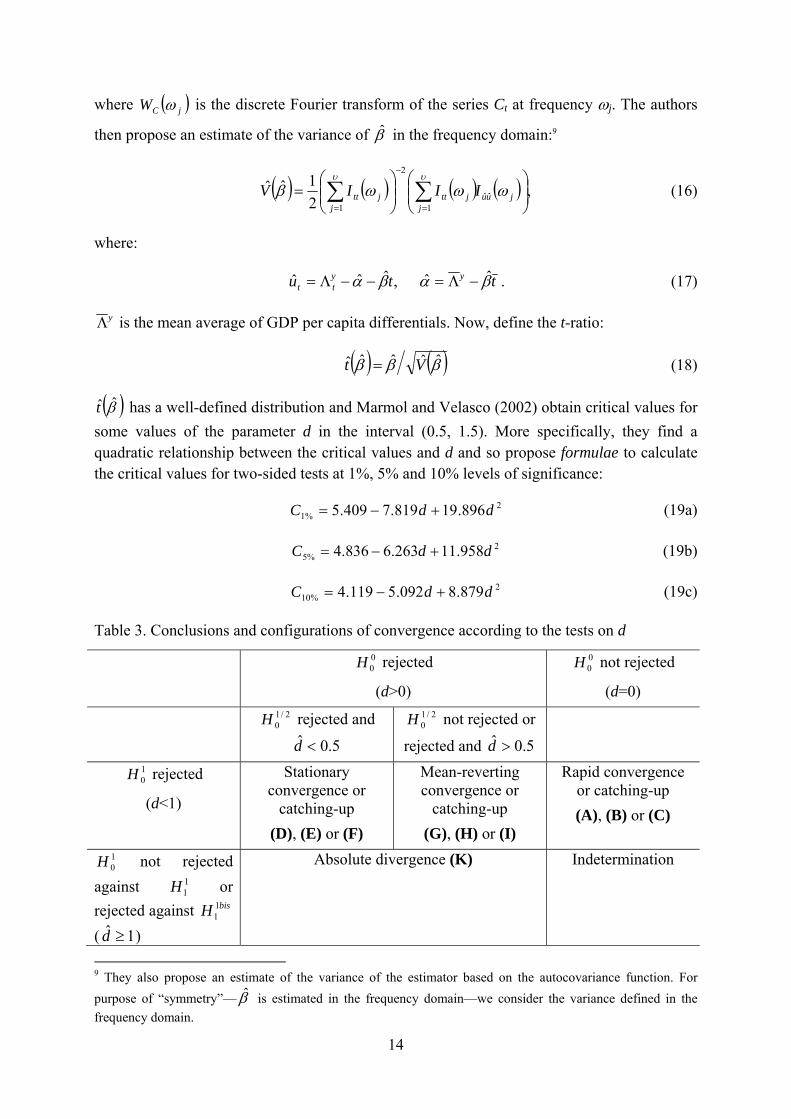
14

where ( )jCW ω is the discrete Fourier transform of the series Ct at frequency ωj. The authors

then propose an estimate of the variance of β̂ in the frequency domain:9

( ) ( ) ( ) ( ) ,21ˆˆ

ˆˆ1

2

1⎟⎟⎠

⎞⎜⎜⎝

⎛⎟⎟⎠

⎞⎜⎜⎝

⎛= ∑∑

=

−

=juu

jjtt

jjtt IIIV ωωωβ

υυ

(16)

where:

ttu yytt βαβα ˆˆ ,ˆˆˆ −Λ=−−Λ= . (17)

yΛ is the mean average of GDP per capita differentials. Now, define the t-ratio:

( ) ( )βββ ˆˆˆˆˆ Vt = (18)

( )β̂t̂ has a well-defined distribution and Marmol and Velasco (2002) obtain critical values for some values of the parameter d in the interval (0.5, 1.5). More specifically, they find a quadratic relationship between the critical values and d and so propose formulae to calculate the critical values for two-sided tests at 1%, 5% and 10% levels of significance:

2%1 896.19819.7409.5 ddC +−= (19a)

2%5 958.11263.6836.4 ddC +−= (19b)

2%10 879.8092.5119.4 ddC +−= (19c)

Table 3. Conclusions and configurations of convergence according to the tests on d

00H rejected

(d>0)

00H not rejected

(d=0) 2/1

0H rejected and

5.0ˆ <d

2/10H not rejected or

rejected and 5.0ˆ >d

10H rejected

(d<1)

Stationary convergence or

catching-up (D), (E) or (F)

Mean-reverting convergence or

catching-up (G), (H) or (I)

Rapid convergence or catching-up (A), (B) or (C)

10H not rejected

against 11H or

rejected against bisH 11

( 1ˆ ≥d )

Absolute divergence (K) Indetermination

9 They also propose an estimate of the variance of the estimator based on the autocovariance function. For purpose of “symmetry”— β̂ is estimated in the frequency domain—we consider the variance defined in the frequency domain.

15

3.2.3. The empirical results: evidence of slow growth convergence

Our data consists of annual GDP per capita series for the period 1950-2006, taken from Madison (2008). We consider 98 developing countries in Africa, Asia and Latin America. Given the large number of countries and the wide variation in the data, we consider 11 subgroups of countries. The subgroups are based on the usual classification made by the International Monetary Fund’s regional economic outlook documents. The criterion is firstly geographical and then within each continent, countries are grouped according to different criteria (oil producers, regional economic areas, fragile states, emerging economies…). The list of countries is presented in Appendix A. For each group, we choose a benchmark country towards which convergence is tested. The benchmark countries are the following: (i) Brazil for South American countries, Panama for Central America, and Puerto-Rico for the Caribbean, (ii) Angola for oil-exporting African countries, Botswana for middle-income African countries, Kenya for low-income African countries, and Sao Tome for fragile Sub-Saharan African countries, (iii) Singapore for new industrialized Asian countries, Thailand for the Asian 5 countries, Pakistan for the other Asian countries, and Israel for Middle-East countries. The benchmark countries are those with the highest per capita real GDP in their sub-sample over the last five years. The output differential series is defined by:

jt

it

yt YY −=Λ (20)

where itY is the logarithm of country i’s GDP per capita and j

tY is the logarithm of the GDP per capita of the benchmark country j.

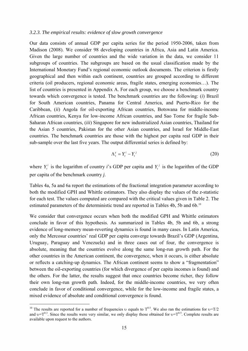
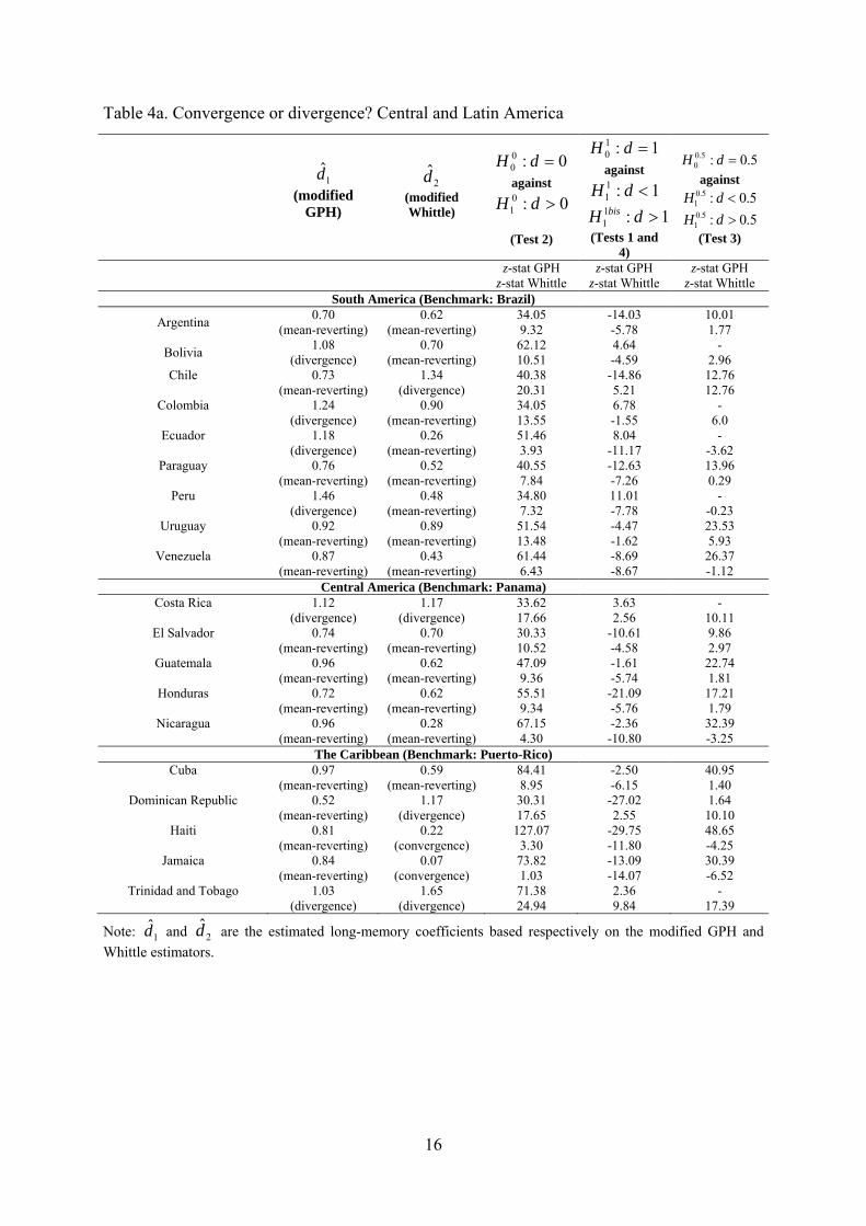
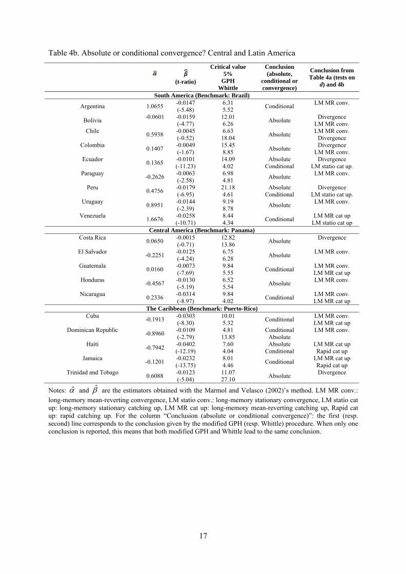
Tables 4a, 5a and 6a report the estimations of the fractional integration parameter according to both the modified GPH and Whittle estimators. They also display the values of the z-statistic for each test. The values computed are compared with the critical values given in Table 2. The estimated parameters of the deterministic trend are reported in Tables 4b, 5b and 6b.10

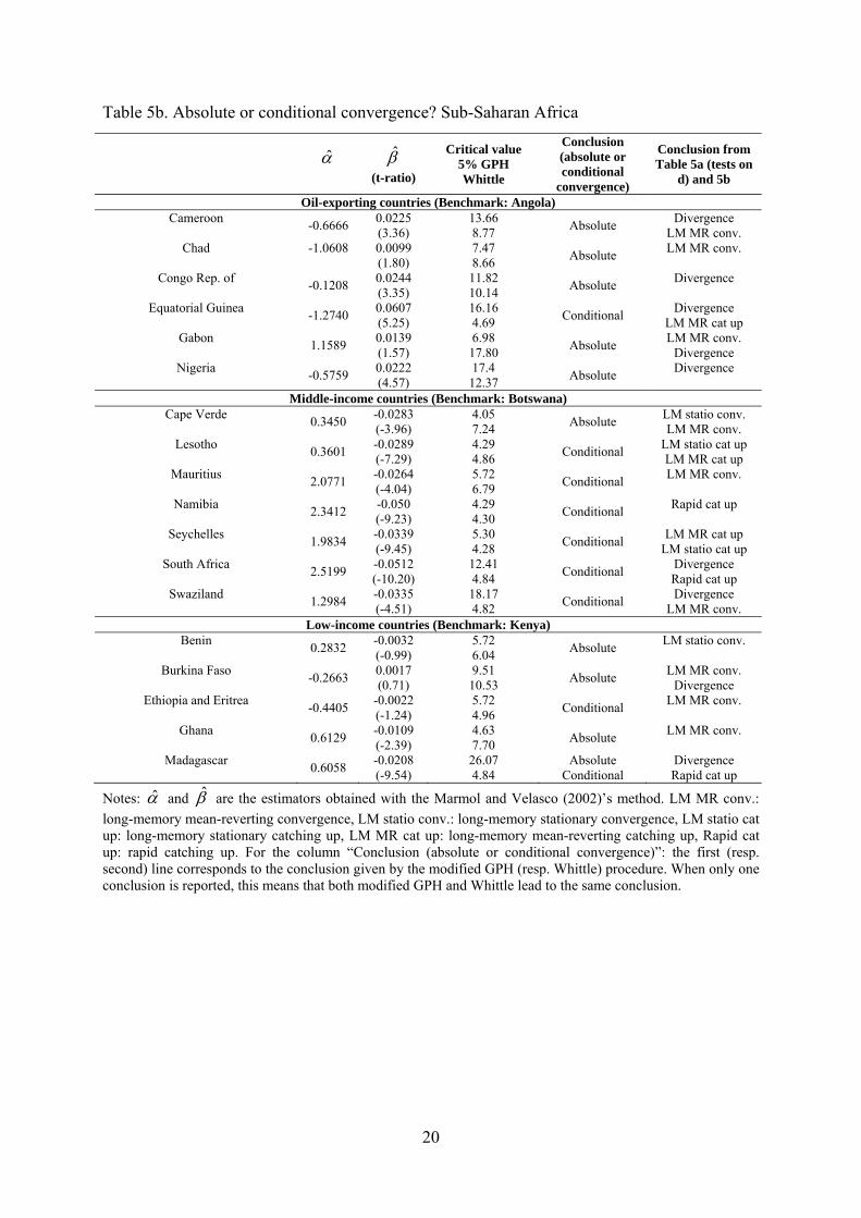
We consider that convergence occurs when both the modified GPH and Whittle estimators conclude in favor of this hypothesis. As summarized in Tables 4b, 5b and 6b, a strong evidence of long-memory mean-reverting dynamics is found in many cases. In Latin America, only the Mercosur countries’ real GDP per capita converge towards Brazil’s GDP (Argentina, Uruguay, Paraguay and Venezuela) and in three cases out of four, the convergence is absolute, meaning that the countries evolve along the same long-run growth path. For the other countries in the American continent, the convergence, when it occurs, is either absolute or reflects a catching-up dynamics. The African continent seems to show a “fragmentation” between the oil-exporting countries (for which divergence of per capita incomes is found) and the others. For the latter, the results suggest that once countries become richer, they follow their own long-run growth path. Indeed, for the middle-income countries, we very often conclude in favor of conditional convergence, while for the low-income and fragile states, a mixed evidence of absolute and conditional convergence is found. 10 The results are reported for a number of frequencies υ equals to T0.5. We also ran the estimations for υ=T/2 and υ=T0.3. Since the results were very similar, we only display those obtained for υ=T0.5. Complete results are available upon request to the authors.

16

Table 4a. Convergence or divergence? Central and Latin America

1d̂

(modified GPH)

2d̂ (modified Whittle)

0:00 =dHagainst

0:01 >dH

(Test 2)

1:10 =dHagainst

1:11 <dH

1:11 >dH bis

(Tests 1 and 4)

5.0:5.00 =dHagainst

5.0:5.01 <dH

5.0:5.01 >dH (Test 3)

z-stat GPH z-stat Whittle



South America (Benchmark: Brazil)

Argentina 0.70 (mean-reverting)

0.62 (mean-reverting)

34.05 9.32

-14.03 -5.78

10.01 1.77

Bolivia 1.08 (divergence)


62.12 10.51

4.64 -4.59

- 2.96

Chile


1.34 (divergence)

40.38 20.31

-14.86 5.21

12.76 12.76

Colombia

1.24 (divergence)


34.05 13.55

6.78 -1.55

- 6.0

Ecuador

1.18 (divergence)


51.46 3.93

8.04 -11.17

- -3.62

Paraguay



40.55 7.84

-12.63 -7.26

13.96 0.29

Peru

1.46 (divergence)


34.80 7.32

11.01 -7.78

- -0.23

Uruguay



51.54 13.48

-4.47 -1.62

23.53 5.93

Venezuela



61.44 6.43

-8.69 -8.67

26.37 -1.12

Central America (Benchmark: Panama)Costa Rica

1.12

(divergence) 1.17

(divergence) 33.62 17.66

3.63 2.56

- 10.11

El Salvador



30.33 10.52

-10.61 -4.58

9.86 2.97

Guatemala



47.09 9.36

-1.61 -5.74

22.74 1.81

Honduras



55.51 9.34

-21.09 -5.76

17.21 1.79

Nicaragua



67.15 4.30

-2.36 -10.80

32.39 -3.25

The Caribbean (Benchmark: Puerto-Rico)Cuba

0.97

(mean-reverting) 0.59

(mean-reverting) 84.41 8.95

-2.50 -6.15

40.95 1.40

Dominican Republic


1.17 (divergence)

30.31 17.65

-27.02 2.55

1.64 10.10

Haiti


0.22 (convergence)

127.07 3.30

-29.75 -11.80

48.65 -4.25

Jamaica


0.07 (convergence)

73.82 1.03

-13.09 -14.07

30.39 -6.52

Trinidad and Tobago

1.03 (divergence)

1.65 (divergence)

71.38 24.94

2.36 9.84

- 17.39

Note: 1d̂ and 2d̂ are the estimated long-memory coefficients based respectively on the modified GPH and Whittle estimators.

17

Table 4b. Absolute or conditional convergence? Central and Latin America

(t-ratio)

Critical value 5%

GPH Whittle

Conclusion (absolute,

conditional or convergence)

Conclusion from Table 4a (tests on

d) and 4b


Argentina 1.0655 -0.0147 (-5.48)

6.31 5.52 Conditional LM MR conv.

Bolivia -0.0601

-0.0159 (-4.77)

12.01 6.26 Absolute Divergence

LM MR conv. Chile

0.5938 -0.0045 (-0.52)

6.63 18.04 Absolute LM MR conv.

Divergence Colombia

0.1407 -0.0049 (-1.67)


LM MR conv. Ecuador

0.1365 -0.0101 (-11.23)

14.09 4.02

Absolute Conditional

Divergence LM statio cat up.

Paraguay -0.2626 -0.0063

(-2.58) 6.98 4.81 Absolute LM MR conv.

Peru

0.4756 -0.0179 (-6.95)

21.18 4.61


Divergence LM statio cat up.

Uruguay 0.8951 -0.0144


Venezuela

1.6676 -0.0258 (-10.71)

8.44 4.34 Conditional LM MR cat up

LM statio cat up Central America (Benchmark: Panama)

Costa Rica 0.0650 -0.0015

(-0.71) 12.82 13.86 Absolute Divergence

El Salvador

-0.2251 -0.0125 (-4.24)


Guatemala

0.0160 -0.0073 (-7.69)


LM MR cat up Honduras

-0.4567 -0.0130 (-5.19)


Nicaragua

0.2336 -0.0314 (-8.97)


LM MR cat up The Caribbean (Benchmark: Puerto-Rico)

Cuba -0.1913 -0.0303

(-8.30) 10.01 5.32 Conditional LM MR conv.

LM MR cat up Dominican Republic

-0.8960 -0.0109 (-2.79)

4.81 13.85

Conditional Absolute

LM MR conv.

Haiti -0.7942 -0.0402

(-12.19) 7.60 4.04


LM MR cat up Rapid cat up

Jamaica -0.1201 -0.0232

(-13.75) 8.01 4.46 Conditional LM MR cat up

Rapid cat up Trinidad and Tobago

0.6088 -0.0123 (-5.04)


Notes: α̂ and β̂ are the estimators obtained with the Marmol and Velasco (2002)’s method. LM MR conv.: long-memory mean-reverting convergence, LM statio conv.: long-memory stationary convergence, LM statio cat up: long-memory stationary catching up, LM MR cat up: long-memory mean-reverting catching up, Rapid cat up: rapid catching up. For the column “Conclusion (absolute or conditional convergence)”: the first (resp. second) line corresponds to the conclusion given by the modified GPH (resp. Whittle) procedure. When only one conclusion is reported, this means that both modified GPH and Whittle lead to the same conclusion.

18

Table 5a. Convergence or divergence? Sub-Saharan Africa

1d̂

(modified GPH)


0:00 =dHagainst

0:01 >dH

(Test 2)

1:10 =dHagainst

1:11 <dH

1:11 >dH bis

(Tests 1 and 4)

5.0:5.00 =dHagainst

5.0:5.01 <dH

5.0:5.01 >dH (Test 3)




Oil-exporting countries (Benchmark: Angola)Cameroon

1.16

(divergence) 0.89


3.98 -1.62

- 5.93

Chad

0.80 (convergence)


19.82 13.37

-4.90 -1.73

7.45 5.82

Congo Rep. of

1.07 (divergence)

0.98 (divergence)

27.53 14.76

2.03 -0.34

- 7.21

Equatorial Guinea

1.27 (divergence)


82.57 7.54

17.53 -7.56

- -0.01

Gabon

0.76 (convergence)

1.34 (divergence)

20.76 20.16

-6.49 5.06

7.13 12.61

Nigeria

1.32 (divergence)

1.10 (divergence)

36.84 16.58

9.01 1.48

- 9.03

Middle-income countries (Benchmark: Botswana)Cape Verde

0.32

(convergence) 0.78


17.73 -3.30

-23.51 4.25

Lesotho

0.40 (convergence)


52.01 7.97

6.90 -7.13

-12.66 0.42

Mauritius



38.97 11.23

-21.70 -3.87

8.63 3.68

Namibia

0.11 (convergence)

0.11 (convergence)

3.65 1.62

11.49 -13.48

-12.00 -5.93

Seychelles



67.67 6.20

0.13 -8.90

11.10 -1.35

South Africa

1.10 (divergence)

0 (convergence)

137.72 0

12.70 -15.10

- -7.55

Swaziland

1.35 (divergence)


58.67 7.87

15.32 -7.23

- 0.32

Low-income countries (Benchmark: Kenya)Benin

0.64

(convergence) 0.67


-8.64 -4.92

3.65 2.63

Burkina Faso


1.0 (divergence)

34.90 15.10

-2.02 0

16.44 7.55

Ethiopia and Eritrea

0.64 (convergence)


22.10 8.21

-12.39 -6.89

4.85 0.66

Ghana

0.49 (convergence)


15.88 12.33

- -2.77

-0.24 4.78

Madagascar

1.62 (divergence)

0 (convergence)

50.77 0

19.58 -15.10

- -7.55


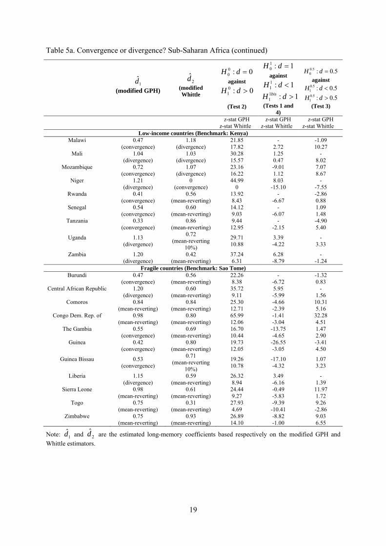
19

Table 5a. Convergence or divergence? Sub-Saharan Africa (continued)

1d̂

(modified GPH)

2d̂ (modified Whittle

0:00 =dHagainst

0:01 >dH

(Test 2)

1:10 =dHagainst

1:11 <dH

1:11 >dH bis

(Tests 1 and 4)

5.0:5.00 =dHagainst

5.0:5.01 <dH

5.0:5.01 >dH (Test 3)




Low-income countries (Benchmark: Kenya)Malawi

0.47

(convergence) 1.18


- 2.72

-1.09 10.27

Mali

1.04 (divergence)

1.03 (divergence)

30.28 15.57

1.25 0.47

- 8.02

Mozambique

0.72 (convergence)

1.07 (divergence)

23.16 16.22

-9.01 1.12

7.07 8.67

Niger

1.21 (divergence)

0 (convergence)

44.99 0

8.03 -15.10

- -7.55

Rwanda

0.41 (convergence)


13.92 8.43

- -6.67

-2.86 0.88

Senegal

0.54 (convergence)


14.12 9.03

- -6.07

1.09 1.48

Tanzania

0.33 (convergence)


9.44 12.95

- -2.15

-4.90 5.40

Uganda

1.13 (divergence)

0.72 (mean-reverting

10%)

29.71 10.88

3.39 -4.22

- 3.33

Zambia

1.20 (divergence)


37.24 6.31

6.28 -8.79

- -1.24

Fragile countries (Benchmark: Sao Tome)Burundi

0.47

(convergence) 0.56


- -6.72

-1.32 0.83

Central African Republic

1.20 (divergence)


35.72 9.11

5.95 -5.99

- 1.56

Comoros



25.30 12.71

-4.66 -2.39

10.31 5.16

Congo Dem. Rep. of



65.99 12.06

-1.41 -3.04

32.28 4.51

The Gambia

0.55 (convergence)


16.70 10.44

-13.75 -4.65

1.47 2.90

Guinea

0.42 (convergence)


19.73 12.05

-26.55 -3.05

-3.41 4.50

Guinea Bissau

0.53 (convergence)


10%)

19.26 10.78

-17.10 -4.32

1.07 3.23

Liberia

1.15 (divergence)


26.32 8.94

3.49 -6.16

- 1.39

Sierra Leone



24.44 9.27

-0.49 -5.83

11.97 1.72

Togo



27.93 4.69

-9.39 -10.41

9.26 -2.86

Zimbabwe



26.89 14.10

-8.82 -1.00

9.03 6.55


20

Table 5b. Absolute or conditional convergence? Sub-Saharan Africa

α̂

β̂ (t-ratio)

Critical value 5% GPH Whittle

Conclusion (absolute or conditional

convergence)


d) and 5b

Oil-exporting countries (Benchmark: Angola)Cameroon

-0.6666 0.0225 (3.36)


LM MR conv. Chad

-1.0608

0.0099 (1.80)


Congo Rep. of

-0.1208 0.0244 (3.35)


Equatorial Guinea

-1.2740 0.0607 (5.25)

16.16 4.69 Conditional Divergence

LM MR cat up Gabon

1.1589 0.0139 (1.57)


Divergence Nigeria

-0.5759 0.0222 (4.57)


Middle-income countries (Benchmark: Botswana)

Cape Verde 0.3450 -0.0283

(-3.96) 4.05 7.24 Absolute LM statio conv.

LM MR conv. Lesotho

0.3601 -0.0289 (-7.29)

4.29 4.86 Conditional LM statio cat up

LM MR cat up Mauritius

2.0771 -0.0264 (-4.04)


Namibia

2.3412 -0.050 (-9.23)

4.29 4.30 Conditional Rapid cat up

Seychelles

1.9834 -0.0339 (-9.45)

5.30 4.28 Conditional LM MR cat up

LM statio cat up South Africa

2.5199 -0.0512 (-10.20)


Rapid cat up Swaziland

1.2984 -0.0335 (-4.51)


LM MR conv. Low-income countries (Benchmark: Kenya)

Benin 0.2832 -0.0032

(-0.99) 5.72 6.04 Absolute LM statio conv.

Burkina Faso

-0.2663 0.0017 (0.71)


Divergence Ethiopia and Eritrea

-0.4405 -0.0022 (-1.24)


Ghana

0.6129 -0.0109 (-2.39)


Madagascar

0.6058 -0.0208 (-9.54)

26.07 4.84


Divergence Rapid cat up


21

Table 5b. Absolute or conditional convergence? Sub-Saharan Africa (continued)

α̂

β̂ (t-ratio)



convergence)


d) and 5b

Low-income countries (Benchmark: Kenya)Malawi

-0.6644 0.0027 (2.40)

4.53 14.09 Conditional LM statio conv.

Divergence Mali

-0.4418

0.0041 (1.27)


Mozambique

0.6339 -0.0096 (-1.75)


Divergence Niger

0.2057 -0.0188 (-6.71)


Rapid cat up Rwanda

-0.1668 -0.0014 (-0.73)

4.28 5.07 Absolute LM statio conv.

LM MR conv. Senegal

0.7144 -0.0110 (-3.48)


Tanzania

-0.3849 -0.0053 (-3.43)

4.07 8.26


LM statio conv. LM MR conv.

Uganda 0.0155 -0.0092


LM MR conv. Zambia

0.3397 -0.0149 (-4.50)


LM statio conv. Fragile countries (Benchmark: Sao Tome)

Burundi -0.8358 -0.0012

(-0.35) 4.53 5.04 Conditional LM statio conv.

LM MR conv. Central African Republic

0.0455 -0.0200 (-4.51)


LM MR conv. Comoros

-0.1852 -0.0130 (-3.64)


Congo Dem. Rep. of

-0.1208 0.0244 (3.35)


The Gambia

-0.2331 -0.0043 (-1.78)


Guinea

-0.9842 0.0012 (0.29)

4.31 7.45 Conditional LM statio conv.

LM MR conv. Guinea Bissau

-0.6373 0.0010 (0.34)

4.87 6.46


LM MR conv.

Liberia 0.3401 -0.0144

(3.76) 13.44 5.32 Absolute Divergence

LM MR conv. Sierra Leone

0.0605 -0.0153 (-4.86)


Togo

-0.1441 -0.0103 (-5.25)


LM statio cat up Zimbabwe

-0.0809 -0.0001 (-0.06)



22

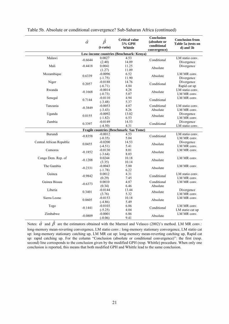
Table 6a. Convergence or divergence? Asia and Middle East

1d̂

(modified GPH)


0:00 =dHagainst

0:01 >dH

(Test 2)

1:10 =dHagainst

1:11 <dH

1:11 >dH bis

(Tests 1 and 4)

5.0:5.00 =dHagainst

5.0:5.01 <dH

5.0:5.01 >dH (Test 3)




New Industrialized Countries (Benchmark: Singapore)Hong-Kong

1.44

(divergence) 1.32


16.35 4.81

- 12.36

South Korea



64.13 12.85

-21.99 -2.25

21.07 5.30

Taiwan

0.69 (convergence)


34.98 10.14

-15.30 -4.96

9.83 2.59

China

0.40 (convergence)

1.20 (divergence)

23.69 18.06

- 2.96

-5.81 10.51

India

0.58 (convergence)


35.63 9.71

-25.31 -5.39

5.16 2.16

Asian 5 (Benchmark: Thailand)Indonesia

1.07

(divergence) 0.59


5.82 -6.12

- 1.43

Malaysia



41.09 9.95

-19.06 -5.15

11.01 2.40

Philippines

0.34 (convergence)


25.81 6.84

- -8.26

-11.29 -0.71

Vietnam



10%)

57.04 11.29

-3.65 -3.80

26.71 3.74

Others (Benchmark: Pakistan)

Bangladesh



10%)

50.82 10.97

-15.15 -4.13

17.83 3.42

Burma

1.19 (divergence)


45.25 10.42

7.39 -4.68

- 2.87

Nepal



57.46 8.86

-13.95 -6.24

21.75 1.31

Sri-Lanka

0.38 (convergence)

1.26 (divergence)

15.06 18.99

- 3.89

-4.71 11.44

Afghanistan

0.13 (convergence)


23.22 6.45

- -8.65

-63.80 -1.10

Cambodia

0.0 (convergence)


- 9.53

- -5.57

- 1.98

Laos

0.17 (convergence)


1.38 11.63

- -3.47

-2.72 4.08

Mongolia


0.98 (divergence)

49.00 14.76

-16.54 -0.34

16.23 7.21

North Korea

1.52 (divergence)


57.67 13.65

19.89 -1.45

- 6.10


23

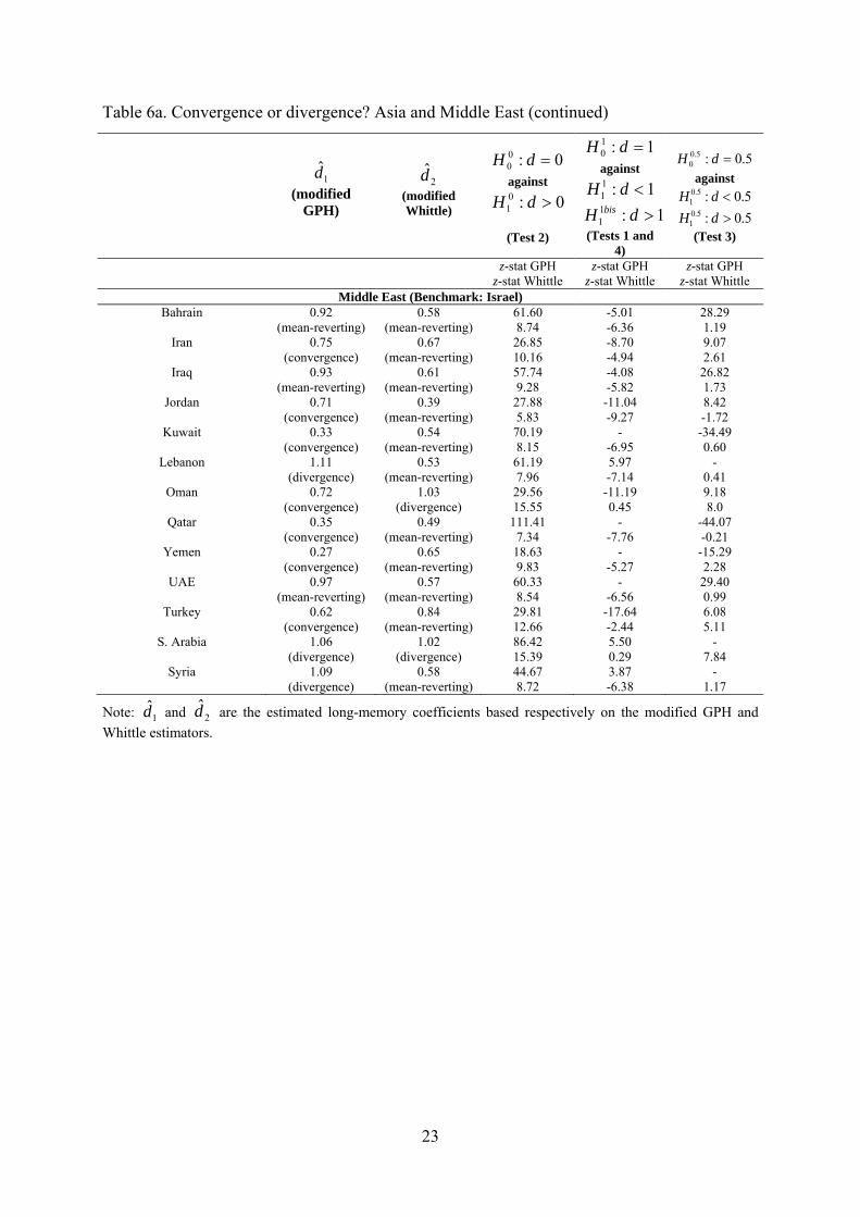
Table 6a. Convergence or divergence? Asia and Middle East (continued)

1d̂

(modified GPH)


0:00 =dHagainst

0:01 >dH

(Test 2)

1:10 =dHagainst

1:11 <dH

1:11 >dH bis

(Tests 1 and 4)

5.0:5.00 =dHagainst

5.0:5.01 <dH

5.0:5.01 >dH (Test 3)




Middle East (Benchmark: Israel)Bahrain

0.92

(mean-reverting) 0.58


-5.01 -6.36

28.29 1.19

Iran

0.75 (convergence)


26.85 10.16

-8.70 -4.94

9.07 2.61

Iraq



57.74 9.28

-4.08 -5.82

26.82 1.73

Jordan

0.71 (convergence)


27.88 5.83

-11.04 -9.27

8.42 -1.72

Kuwait

0.33 (convergence)


70.19 8.15

- -6.95

-34.49 0.60

Lebanon

1.11 (divergence)


61.19 7.96

5.97 -7.14

- 0.41

Oman

0.72 (convergence)

1.03 (divergence)

29.56 15.55

-11.19 0.45

9.18 8.0

Qatar

0.35 (convergence)


111.41 7.34

- -7.76

-44.07 -0.21

Yemen

0.27 (convergence)


18.63 9.83

- -5.27

-15.29 2.28

UAE



60.33 8.54

- -6.56

29.40 0.99

Turkey

0.62 (convergence)


29.81 12.66

-17.64 -2.44

6.08 5.11

S. Arabia

1.06 (divergence)

1.02 (divergence)

86.42 15.39

5.50 0.29

- 7.84

Syria

1.09 (divergence)


44.67 8.72

3.87 -6.38

- 1.17


24

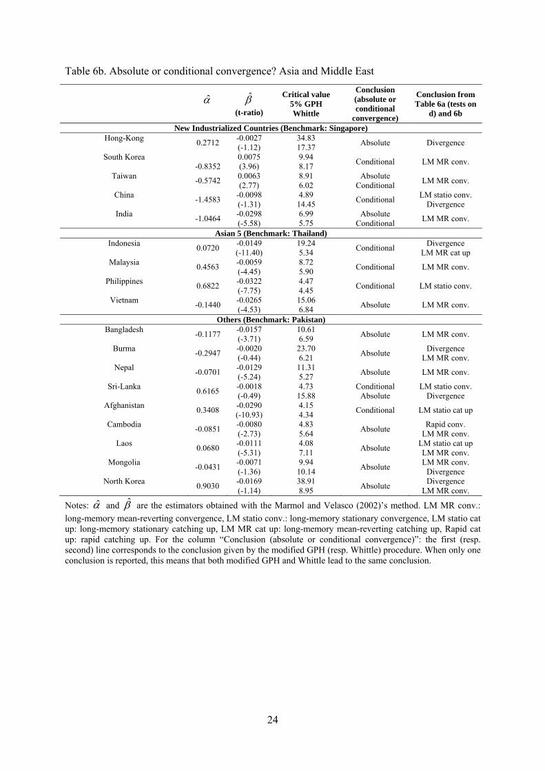
Table 6b. Absolute or conditional convergence? Asia and Middle East

α̂

β̂ (t-ratio)



convergence)


d) and 6b

New Industrialized Countries (Benchmark: Singapore)Hong-Kong

0.2712 -0.0027 (-1.12)


South Korea

-0.8352

0.0075 (3.96)


Taiwan -0.5742 0.0063

(2.77) 8.91 6.02

Absolute Conditional LM MR conv.

China -1.4583 -0.0098


Divergence India

-1.0464 -0.0298 (-5.58)

6.99 5.75

Absolute Conditional LM MR conv.

Asian 5 (Benchmark: Thailand)Indonesia

0.0720 -0.0149 (-11.40)


LM MR cat up Malaysia

0.4563 -0.0059 (-4.45)


Philippines 0.6822 -0.0322


Vietnam -0.1440 -0.0265


Others (Benchmark: Pakistan)Bangladesh

-0.1177 -0.0157 (-3.71)


Burma -0.2947 -0.0020


LM MR conv. Nepal

-0.0701 -0.0129 (-5.24)


Sri-Lanka 0.6165 -0.0018

(-0.49) 4.73 15.88


LM statio conv. Divergence

Afghanistan 0.3408 -0.0290

(-10.93) 4.15 4.34 Conditional LM statio cat up

Cambodia -0.0851 -0.0080

(-2.73) 4.83 5.64 Absolute Rapid conv.

LM MR conv. Laos

0.0680 -0.0111 (-5.31)

4.08 7.11 Absolute LM statio cat up

LM MR conv. Mongolia

-0.0431 -0.0071 (-1.36)


Divergence North Korea

0.9030 -0.0169 (-1.14)


LM MR conv.


25

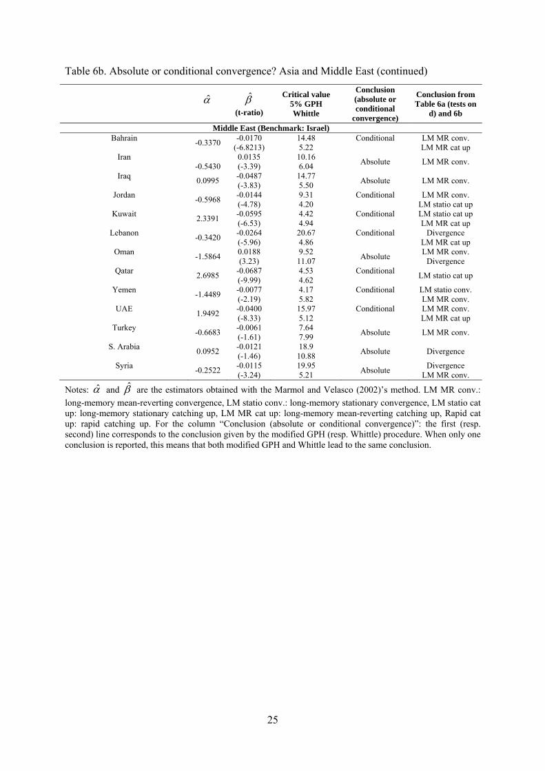
Table 6b. Absolute or conditional convergence? Asia and Middle East (continued)

α̂

β̂ (t-ratio)



convergence)


d) and 6b

Middle East (Benchmark: Israel)Bahrain

-0.3370 -0.0170 (-6.8213)

14.48 5.22

Conditional

LM MR conv. LM MR cat up

Iran

-0.5430

0.0135 (-3.39)


Iraq 0.0995 -0.0487


Jordan -0.5968 -0.0144

(-4.78) 9.31 4.20

Conditional

LM MR conv. LM statio cat up

Kuwait 2.3391 -0.0595

(-6.53) 4.42 4.94

Conditional

LM statio cat up LM MR cat up

Lebanon -0.3420 -0.0264

(-5.96) 20.67 4.86

Conditional

Divergence LM MR cat up

Oman -1.5864 0.0188

(3.23) 9.52 11.07 Absolute LM MR conv.

Divergence Qatar

2.6985 -0.0687 (-9.99)

4.53 4.62

Conditional LM statio cat up

Yemen -1.4489 -0.0077

(-2.19) 4.17 5.82

Conditional

LM statio conv. LM MR conv.

UAE 1.9492 -0.0400

(-8.33) 15.97 5.12

Conditional

LM MR conv. LM MR cat up

Turkey -0.6683 -0.0061


S. Arabia 0.0952 -0.0121


Syria -0.2522 -0.0115


LM MR conv.


26

The same conclusion seems to hold for Asia and the Middle-East. For the richest countries (be they newly industrialized countries, Asian 5 or oil-producers in the Middle East), we frequently find a conditional convergence, while for the group of the other countries we mainly conclude in favor of absolute convergence. This is an interesting finding. Indeed, if we assume that the type of convergence depends upon the level of income, then our results would suggest that, for the poorest countries to grow faster than the richest ones (a consequence of catching-up or conditional convergence), countries must first achieve a minimum level of wealth. In the samples involving very poor (low-income) countries, each nation tends instead to approach the same steady state (absolute convergence). This happens probably because no significant differences are observed in their technological and economic fundamentals (low productivity growth, low level of human capital, etc.). Technological transfers across countries only occur in addition to prior accumulation of capital, minimum saving rates, etc.

The estimates of the long-memory parameter (Tables 4a, 5a and 6a) are neither negative, nor statistically equal to zero (with both methods), but many take a value between 0.5 and 1. It means that per capita income differential series exhibit a non-stationary long-memory dynamics over time.

Several arguments could be evoked to explain our finding of a persistent (long-memory) and non-stationary dynamics of the per capita output differentials. One explanation may be that some countries stay backward, falling in a self-reinforcing vicious circle of poverty trap corresponding to convergence to low levels of income (see Section 4 below). This would apply for instance to the low-income countries and fragile states in Africa, but also to the poorest countries in Asia (Cambodia, Afghanistan, Sri-Lanka, North Korea, Mongolia). In these cases, the findings of a slow convergence could mean that income is not mainly influenced by economic fundamentals (infrastructure, education, productivity, etc.), but by historical accidents.11

Another argument that may explain our finding of catching-up paths with non-stationary long-memory dynamics during the transition to long-run growth is the existence of multiple equilibria, as described for instance by the Schumpeterian models of evolutionary economic growth or by the structuralist evolutionary models.12 This argument could apply to the richest countries in our samples (the middle-income countries in Africa, the New Industrialized Economies in Asia, Asian 5 and the Middle-East countries). Indeed, the growth dynamics not only implies quantitative, but also qualitative changes. The choice of a technology or of a consumption fashion at a given time is endogenously determined by decisions taken by agents in search of a new equilibrium. By equilibrium, it is meant the state of technology, knowledge, institutions and markets, social relationships, etc. Because individuals face uncertainty when making their choices, there are different possible outcomes that cannot be determined in advance. This leads to a path-dependent dynamics implying more or less rigidity or inertia. Such “search dynamics” are well described by nonlinear models, for instance Markov-switching models that attribute probabilities to alternative future states, or 11 See Landes (1998). 12 See, among others, Nelson and Winter (1982) and Lipsey, Carlaw and Bekar (2005).

27

by structural change models like TAR (Threshold Autoregressive) or STAR (Smooth Transition Autoregressive) models. It has been demonstrated in the literature that these processes exhibit properties that are very similar to those of long-memory models.13

3.2.4. Robustness to an alternative method: wavelet estimator

We check the robustness of our empirical findings to an alternative methodology based on wavelet analysis.14 Wavelet analysis allows us to simultaneously localize a process in time and scale. High scales are associated with short lived time phenomena, while low scales concern the long run behavior. A wavelet OLS estimator of the fractional differencing parameter d in an ARFIMA(0,d,0) was proposed by Jensen (1999), based on a log-linear relationship between the variance of the wavelet coefficients and the scaling parameter equal to d. The methodology can be summarized as follows.

Firstly, we apply the discrete wavelet transform to the per capita GDP and obtain the following wavelet coefficients:

( ) )(,,...,,0021 tWcwww y

jj Λ×= (21)

where iw are the wavelet coefficients vectors which correspond to the high frequency

components of )(tyΛ , 0j

c is the scale coefficient vector which corresponds to the low

frequency component of )(tyΛ , 0j denotes the number of levels of the decomposition (at each level corresponds a time scale of the decomposition) and W is the wavelet matrix, which rows are made of the chosen wavelet and scale filter coefficients. W corresponds to the matrix of an orthonormal basis of functions )(

0tkjφ and )(tjkψ , respectively known as the scaling and

wavelet functions, on which the vector )(tyΛ is projected.

In a second step, we compute the variance of the wavelet coefficients at each scale j:

( ) ∑−

=Λ =

12/22

21 j

j

T

Lkjk

jjj w

Tλλσ) (22)

where jλ is the scale of level j (here 12 −j ), ( )( )[ ]1112 +−−= LFloorL jj is the number of

wavelet coefficients affected by boundary conditions, and jT is the number of wavelet

coefficients not affected by them.15 Jensen (1999) shows that there exists a linear relationship

13 See for instance Diebold and Inoue (2001), Kapetanios, Shin and Snell (2003). 14 For an overview of wavelet analysis, see Percival and Walden (2000). 15 As with any filter, boundary issues emerge when calculating wavelet coefficients at the ends of the observation vector. To solve this problem, the time series were reflected about their last observations. In order to avoid any bias due to these added observations, it is important to keep track of them. Percival and Walden (2000) showed that the number of coefficients not affected by boundary conditions is given by ( )( )[ ]jj

j LFloorTT −−−−= 2122/ , where L is the length of the considered filter and Floor(x) denotes the greatest integer less than or equal to x.

28

between the scale jλ and the wavelet variance ( )jλσ 2Λ) and proves that

( ) 122 −∞→⎯⎯ →⎯ d

jjjx Cλλσ) . Accordingly, he suggests the following OLS regression to estimate d:

( )( ) ( ) jjj e++=Λ λββλσ loglog 102) ,

( )2

11 +=β)

)d (23)

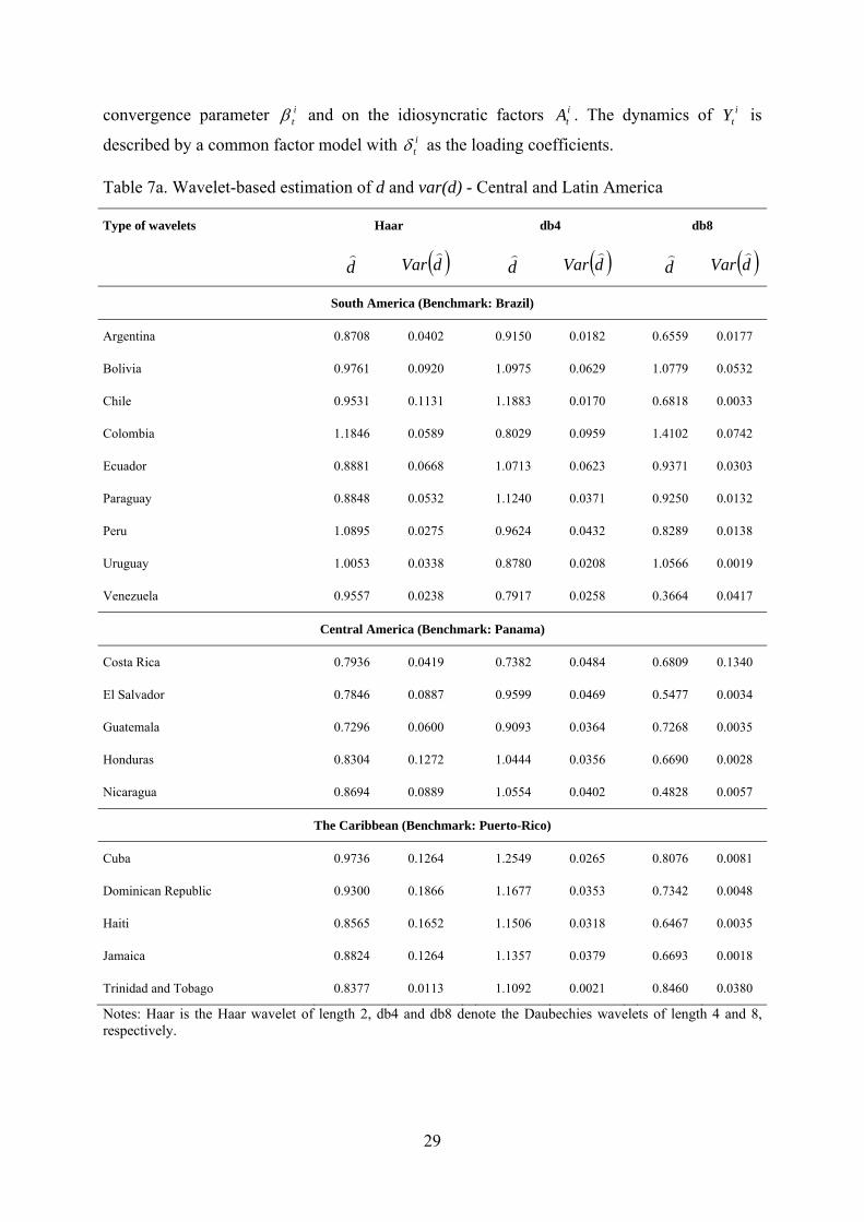
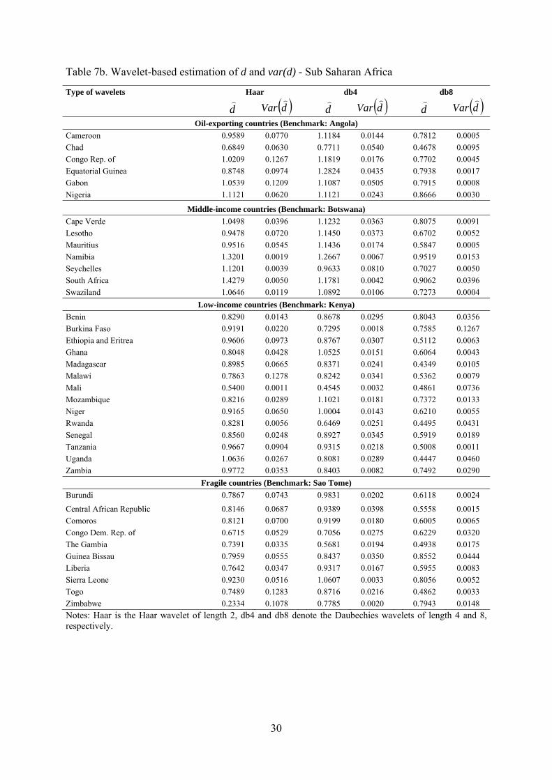
Tables 7a to 7c display our estimates of d and its variance using three wavelets functions: the Haar wavelet and the Daubechies wavelets with four and eight vanishing moments. The estimates unambiguously confirm evidence of long-memory, putting forward a very persistent dynamics in the per capita GDP differentials. The conclusions are robust to changes in the Daubechies smoothing parameter. On the whole, our results using either the modified GPH and Whittle estimators or the wavelet procedure, thus show that growth convergence follows a mean-reverting persistent process in many cases.

4. Modelling the slowly varying transition paths to long-run growth

We have just found that growth convergence between the developing countries is characterized by a slow mean-reverting and non-stationary dynamics. In this section, we go a step further by modeling the slowly varying transition paths to long-run equilibrium, relying upon the time-varying factor representation proposed by Phillips and Sul (2007a, 2007b).

The economic background of the econometric methodology is the reduced form of a Solow growth model allowing for heterogeneous speeds of convergence and transition effects over time:

( ) tAaAeYYYY it

it

it

tiiiit

it +=+−+= −β*

0* (24)

with

( ) tiiiit

iteYYYa β−−+= *

0* (25)

itY is the log of per capita GDP in country i at time t, *iY is the log of the steady-state level of

per capita GDP, and iY0 denotes the log of the initial per capita GDP. itβ is the time-varying

speed of convergence rate and itA is a vector of variables conditioning growth (institutions,

geography, saving rate, human capital, history, etc.). Assume that the countries share common elements tμ that promote growth, for instance technology. i

tY can be written as follows:

titt

t

it

iti

ttAa

Y μδμμ

=⎟⎟⎠

⎞⎜⎜⎝

⎛ += (26)

itδ is the time-varying share of the common technology that economy i experiences, or the

transition path to the common steady state determined by tμ . It depends upon the speed of

29

convergence parameter itβ and on the idiosyncratic factors i

tA . The dynamics of itY is

described by a common factor model with itδ as the loading coefficients.

Table 7a. Wavelet-based estimation of d and var(d) - Central and Latin America

Type of wavelets Haar db4 db8

d)

( )dVar)

d)

( )dVar)

d)

( )dVar)


Argentina 0.8708 0.0402 0.9150 0.0182 0.6559 0.0177

Bolivia 0.9761 0.0920 1.0975 0.0629 1.0779 0.0532

Chile 0.9531 0.1131 1.1883 0.0170 0.6818 0.0033

Colombia 1.1846 0.0589 0.8029 0.0959 1.4102 0.0742

Ecuador 0.8881 0.0668 1.0713 0.0623 0.9371 0.0303

Paraguay 0.8848 0.0532 1.1240 0.0371 0.9250 0.0132

Peru 1.0895 0.0275 0.9624 0.0432 0.8289 0.0138

Uruguay 1.0053 0.0338 0.8780 0.0208 1.0566 0.0019

Venezuela 0.9557 0.0238 0.7917 0.0258 0.3664 0.0417

Central America (Benchmark: Panama)

Costa Rica 0.7936 0.0419 0.7382 0.0484 0.6809 0.1340

El Salvador 0.7846 0.0887 0.9599 0.0469 0.5477 0.0034

Guatemala 0.7296 0.0600 0.9093 0.0364 0.7268 0.0035

Honduras 0.8304 0.1272 1.0444 0.0356 0.6690 0.0028

Nicaragua 0.8694 0.0889 1.0554 0.0402 0.4828 0.0057

The Caribbean (Benchmark: Puerto-Rico)

Cuba 0.9736 0.1264 1.2549 0.0265 0.8076 0.0081

Dominican Republic 0.9300 0.1866 1.1677 0.0353 0.7342 0.0048

Haiti 0.8565 0.1652 1.1506 0.0318 0.6467 0.0035

Jamaica 0.8824 0.1264 1.1357 0.0379 0.6693 0.0018

Trinidad and Tobago 0.8377 0.0113 1.1092 0.0021 0.8460 0.0380

Notes: Haar is the Haar wavelet of length 2, db4 and db8 denote the Daubechies wavelets of length 4 and 8, respectively.

30

Table 7b. Wavelet-based estimation of d and var(d) - Sub Saharan Africa


d)

( )dVar)

d)

( )dVar)

d)

( )dVar)

Oil-exporting countries (Benchmark: Angola) Cameroon 0.9589 0.0770 1.1184 0.0144 0.7812 0.0005 Chad 0.6849 0.0630 0.7711 0.0540 0.4678 0.0095 Congo Rep. of 1.0209 0.1267 1.1819 0.0176 0.7702 0.0045 Equatorial Guinea 0.8748 0.0974 1.2824 0.0435 0.7938 0.0017 Gabon 1.0539 0.1209 1.1087 0.0505 0.7915 0.0008 Nigeria 1.1121 0.0620 1.1121 0.0243 0.8666 0.0030

Middle-income countries (Benchmark: Botswana) Cape Verde 1.0498 0.0396 1.1232 0.0363 0.8075 0.0091 Lesotho 0.9478 0.0720 1.1450 0.0373 0.6702 0.0052 Mauritius 0.9516 0.0545 1.1436 0.0174 0.5847 0.0005 Namibia 1.3201 0.0019 1.2667 0.0067 0.9519 0.0153 Seychelles 1.1201 0.0039 0.9633 0.0810 0.7027 0.0050 South Africa 1.4279 0.0050 1.1781 0.0042 0.9062 0.0396 Swaziland 1.0646 0.0119 1.0892 0.0106 0.7273 0.0004

Low-income countries (Benchmark: Kenya) Benin 0.8290 0.0143 0.8678 0.0295 0.8043 0.0356 Burkina Faso 0.9191 0.0220 0.7295 0.0018 0.7585 0.1267 Ethiopia and Eritrea 0.9606 0.0973 0.8767 0.0307 0.5112 0.0063 Ghana 0.8048 0.0428 1.0525 0.0151 0.6064 0.0043 Madagascar 0.8985 0.0665 0.8371 0.0241 0.4349 0.0105 Malawi 0.7863 0.1278 0.8242 0.0341 0.5362 0.0079 Mali 0.5400 0.0011 0.4545 0.0032 0.4861 0.0736 Mozambique 0.8216 0.0289 1.1021 0.0181 0.7372 0.0133 Niger 0.9165 0.0650 1.0004 0.0143 0.6210 0.0055 Rwanda 0.8281 0.0056 0.6469 0.0251 0.4495 0.0431 Senegal 0.8560 0.0248 0.8927 0.0345 0.5919 0.0189 Tanzania 0.9667 0.0904 0.9315 0.0218 0.5008 0.0011 Uganda 1.0636 0.0267 0.8081 0.0289 0.4447 0.0460 Zambia 0.9772 0.0353 0.8403 0.0082 0.7492 0.0290

Fragile countries (Benchmark: Sao Tome) Burundi 0.7867 0.0743 0.9831 0.0202 0.6118 0.0024

Central African Republic 0.8146 0.0687 0.9389 0.0398 0.5558 0.0015 Comoros 0.8121 0.0700 0.9199 0.0180 0.6005 0.0065 Congo Dem. Rep. of 0.6715 0.0529 0.7056 0.0275 0.6229 0.0320 The Gambia 0.7391 0.0335 0.5681 0.0194 0.4938 0.0175 Guinea Bissau 0.7959 0.0555 0.8437 0.0350 0.8552 0.0444 Liberia 0.7642 0.0347 0.9317 0.0167 0.5955 0.0083 Sierra Leone 0.9230 0.0516 1.0607 0.0033 0.8056 0.0052 Togo 0.7489 0.1283 0.8716 0.0216 0.4862 0.0033 Zimbabwe 0.2334 0.1078 0.7785 0.0020 0.7943 0.0148 Notes: Haar is the Haar wavelet of length 2, db4 and db8 denote the Daubechies wavelets of length 4 and 8, respectively.

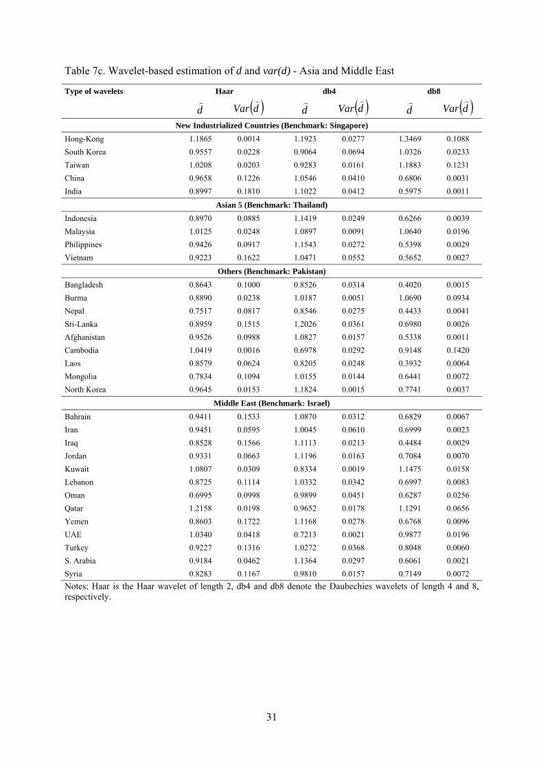
31

Table 7c. Wavelet-based estimation of d and var(d) - Asia and Middle East


d)

( )dVar)

d)

( )dVar)

d)

( )dVar)

New Industrialized Countries (Benchmark: Singapore) Hong-Kong 1.1865 0.0014 1.1923 0.0277 1.3469 0.1088 South Korea 0.9557 0.0228 0.9064 0.0694 1.0326 0.0233 Taiwan 1.0208 0.0203 0.9283 0.0161 1.1883 0.1231 China 0.9658 0.1226 1.0546 0.0410 0.6806 0.0031 India 0.8997 0.1810 1.1022 0.0412 0.5975 0.0011

Asian 5 (Benchmark: Thailand) Indonesia 0.8970 0.0885 1.1419 0.0249 0.6266 0.0039 Malaysia 1.0125 0.0248 1.0897 0.0091 1.0640 0.0196 Philippines 0.9426 0.0917 1.1543 0.0272 0.5398 0.0029 Vietnam 0.9223 0.1622 1.0471 0.0552 0.5652 0.0027

Others (Benchmark: Pakistan) Bangladesh 0.8643 0.1000 0.8526 0.0314 0.4020 0.0015 Burma 0.8890 0.0238 1.0187 0.0051 1.0690 0.0934 Nepal 0.7517 0.0817 0.8546 0.0275 0.4433 0.0041 Sri-Lanka 0.8959 0.1515 1.2026 0.0361 0.6980 0.0026 Afghanistan 0.9526 0.0988 1.0827 0.0157 0.5338 0.0011 Cambodia 1.0419 0.0016 0.6978 0.0292 0.9148 0.1420 Laos 0.8579 0.0624 0.8205 0.0248 0.3932 0.0064 Mongolia 0.7834 0.1094 1.0155 0.0144 0.6441 0.0072 North Korea 0.9645 0.0153 1.1824 0.0015 0.7741 0.0037

Middle East (Benchmark: Israel) Bahrain 0.9411 0.1533 1.0870 0.0312 0.6829 0.0067 Iran 0.9451 0.0595 1.0045 0.0610 0.6999 0.0023 Iraq 0.8528 0.1566 1.1113 0.0213 0.4484 0.0029 Jordan 0.9331 0.0663 1.1196 0.0163 0.7084 0.0070 Kuwait 1.0807 0.0309 0.8334 0.0019 1.1475 0.0158 Lebanon 0.8725 0.1114 1.0332 0.0342 0.6997 0.0083 Oman 0.6995 0.0998 0.9899 0.0451 0.6287 0.0256 Qatar 1.2158 0.0198 0.9652 0.0178 1.1291 0.0656 Yemen 0.8603 0.1722 1.1168 0.0278 0.6768 0.0096 UAE 1.0340 0.0418 0.7213 0.0021 0.9877 0.0196 Turkey 0.9227 0.1316 1.0272 0.0368 0.8048 0.0060 S. Arabia 0.9184 0.0462 1.1364 0.0297 0.6061 0.0021 Syria 0.8283 0.1167 0.9810 0.0157 0.7149 0.0072 Notes: Haar is the Haar wavelet of length 2, db4 and db8 denote the Daubechies wavelets of length 4 and 8, respectively.

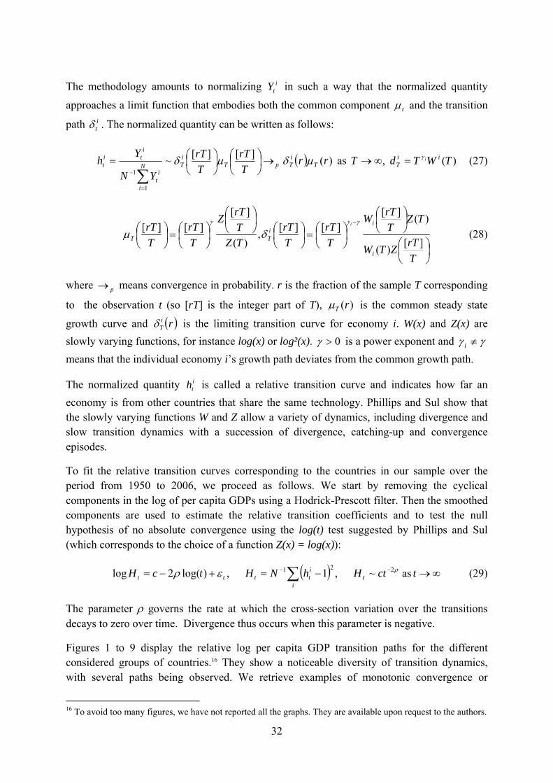
32

The methodology amounts to normalizing i

tY in such a way that the normalized quantity

approaches a limit function that embodies both the common component tμ and the transition

path itδ . The normalized quantity can be written as follows:

( ) )( , as )(][][~

1

1TWTdTrr

TrT

TrT

YN

Yh ii

TTiTpT

iTN

i

it

iti

tiγμδμδ =∞→→⎟

⎠⎞

⎜⎝⎛

⎟⎠⎞

⎜⎝⎛=

∑=

−

(27)

⎟⎠⎞

⎜⎝⎛

⎟⎠⎞

⎜⎝⎛

⎟⎠⎞

⎜⎝⎛=⎟

⎠⎞

⎜⎝⎛

⎟⎠⎞

⎜⎝⎛

⎟⎠⎞

⎜⎝⎛=⎟

⎠⎞

⎜⎝⎛

−

TrTZTW

TZTrTW

TrT

TrT

TZTrTZ

TrT

TrT

i

iiTT

i

][)(

)(][][][,

)(

][][][ γγγ

δμ (28)

where p→ means convergence in probability. r is the fraction of the sample T corresponding

to the observation t (so [rT] is the integer part of T), )(rTμ is the common steady state

growth curve and ( )riTδ is the limiting transition curve for economy i. W(x) and Z(x) are

slowly varying functions, for instance log(x) or log²(x). 0>γ is a power exponent and γγ ≠i means that the individual economy i’s growth path deviates from the common growth path.

The normalized quantity ith is called a relative transition curve and indicates how far an

economy is from other countries that share the same technology. Phillips and Sul show that the slowly varying functions W and Z allow a variety of dynamics, including divergence and slow transition dynamics with a succession of divergence, catching-up and convergence episodes.

To fit the relative transition curves corresponding to the countries in our sample over the period from 1950 to 2006, we proceed as follows. We start by removing the cyclical components in the log of per capita GDPs using a Hodrick-Prescott filter. Then the smoothed components are used to estimate the relative transition coefficients and to test the null hypothesis of no absolute convergence using the log(t) test suggested by Phillips and Sul (which corresponds to the choice of a function Z(x) = log(x)):

( ) ∞→−=+−= −− ∑ tctHhNHtcHi

titttt as ~ ,1 ,)log(2log 221 ρερ (29)

The parameter ρ governs the rate at which the cross-section variation over the transitions decays to zero over time. Divergence thus occurs when this parameter is negative.

Figures 1 to 9 display the relative log per capita GDP transition paths for the different considered groups of countries.16 They show a noticeable diversity of transition dynamics, with several paths being observed. We retrieve examples of monotonic convergence or

16 To avoid too many figures, we have not reported all the graphs. They are available upon request to the authors.

33

divergence (Figure 1, Chile; Figure 2, Costa Rica; Figure 3, Puerto-Rico; Figure 4, subgroup of Asian new industrialized countries; Figure 5, Pakistan). But, in many cases, we observe non-stationary transitional dynamics that differ across countries. Some involve an initial phase of divergence from the group, followed by catch-up and then convergence (Figure 4, China and India; Figure 5, Afghanistan, Bangladesh; Figure 6, Qatar; Figure 7, Cape Verde, Namibia). Figures also reveal that the transition to long-run growth can be characterized by a complex pattern with countries changing their growth performance very often. A typical example is given by Figure 9 which displays the transition paths for the subgroup of the African fragile economies. In many cases, the computed relative coefficients do not show a coherent pattern.

The time profile for the Middle-East countries (Figure 6) shows an example of absolute convergence. Some countries start above average (Qatar, Kuwait) and follow a downward direction, while others start below average and exhibit upward transition (Oman, Jordan, Israel). The log(t) test reported in Table 8 does not reject the null hypothesis of no convergence, thereby implying that, for this subgroup of countries, there is a common factor driving their economies together in the long run. This common factor could be the predominance of oil revenues in the countries’ GDP. But, it does not mean that an important oil sector will be always a driving factor of long-run convergence. The counter-example here is the group of oil-exporting countries in Africa (Figure 7). For this group of countries, the hypothesis of absolute convergence is rejected and the graph suggests conditional convergence with each trajectory leading to a different terminal point (though absolute convergence seems to apply to the subgroup comprising Equatorial Guinea, Cameroon and Nigeria). There is also evidence that many of these countries are converging to a GDP level below average, which is a sign of impoverishment over time. The opposite situation seems to happen for a subgroup of the Asian new industrialized countries since Singapore, Taiwan, Hong-Kong and South-Korea converge to a level above average.

Dramatic situations also occur, which can be associated with “growth tragedy”. As previously mentioned, this expression applies to countries that experience a regression in growth despite the fact that their initial income per capita is far below average. Some examples are Chad, Cameroon, Congo and Equatorial Guinea in Africa; Bolivia, Ecuador, Haiti and Nicaragua in Latin America; Afghanistan, Bangladesh, Laos and Nepal in Asia. Iraq is another example of growth tragedy with a transition curve that is characterized by a catching-up dynamics up until the mid-eighties and then by a collapse after 1985.

One salient feature is that there is no narrowing of the dispersion in the relative transition curves (this illustrates the predominance of conditional convergence). Comparing the trajectories of the countries that are initially above average and those below average, we see that the differences are reduced over time in only but a few cases (Middle-East countries, the subgroup of the Asian Tigers and the middle-income African countries). This clearly indicates no tendency to converge towards the end of the period. This conclusion is confirmed when we perform the log(t) test for the different subgroups of countries. The null of no convergence is rejected when the coefficient ρ is positive and statistically significant. Table 8 shows that we conclude in favor of absolute convergence only for the subgroups of the Middle-East

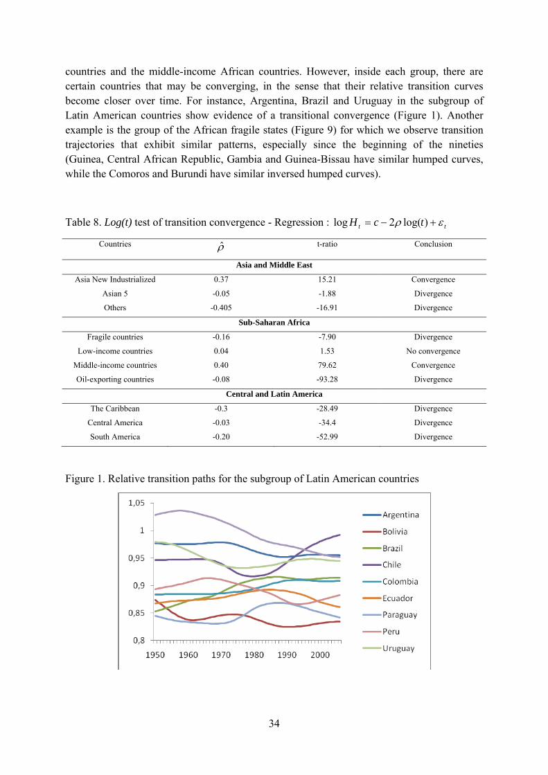
34

countries and the middle-income African countries. However, inside each group, there are certain countries that may be converging, in the sense that their relative transition curves become closer over time. For instance, Argentina, Brazil and Uruguay in the subgroup of Latin American countries show evidence of a transitional convergence (Figure 1). Another example is the group of the African fragile states (Figure 9) for which we observe transition trajectories that exhibit similar patterns, especially since the beginning of the nineties (Guinea, Central African Republic, Gambia and Guinea-Bissau have similar humped curves, while the Comoros and Burundi have similar inversed humped curves).

Table 8. Log(t) test of transition convergence - Regression : tt tcH ερ +−= )log(2log

Countries ρ̂ t-ratio Conclusion

Asia and Middle East

Asia New Industrialized 0.37 15.21 Convergence

Asian 5 -0.05 -1.88 Divergence

Others -0.405 -16.91 Divergence

Sub-Saharan Africa

Fragile countries -0.16 -7.90 Divergence

Low-income countries 0.04 1.53 No convergence

Middle-income countries 0.40 79.62 Convergence

Oil-exporting countries -0.08 -93.28 Divergence

Central and Latin America

The Caribbean -0.3 -28.49 Divergence

Central America -0.03 -34.4 Divergence

South America -0.20 -52.99 Divergence

Figure 1. Relative transition paths for the subgroup of Latin American countries

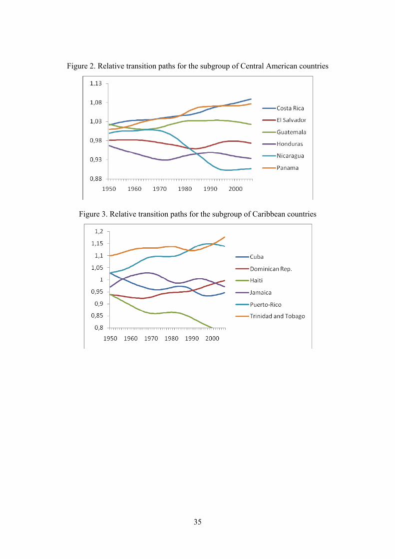
35

Figure 2. Relative transition paths for the subgroup of Central American countries

Figure 3. Relative transition paths for the subgroup of Caribbean countries

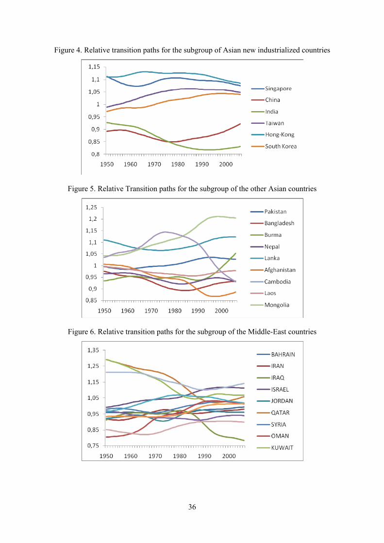
36

Figure 4. Relative transition paths for the subgroup of Asian new industrialized countries

Figure 5. Relative Transition paths for the subgroup of the other Asian countries

Figure 6. Relative transition paths for the subgroup of the Middle-East countries

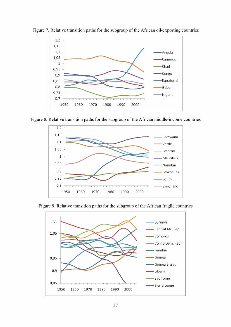
37

Figure 7. Relative transition paths for the subgroup of the African oil-exporting countries

Figure 8. Relative transition paths for the subgroup of the African middle-income countries

Figure 9. Relative transition paths for the subgroup of the African fragile countries

38

5. Conclusion

A central message of our results is that growth convergence in the developing countries is characterized by a slow transition dynamics and by complex paths involving non-stationary behaviors. These findings provide an empirical support to the theoretical conjecture that growth in the developing countries may be characterized by heterochronic changes and should re-energize research based on biological models of economic growth. The basic idea is that the organizational process underlying growth (government policies, industry clusters, market organization, civil relationships, etc.) goes through varying stages, has varying permutations of new and old institutional relationships and strikes differently according to cultural, history and political systems. This creates complex transition episodes and more or less persistent dynamics that operate across multiple time scales. In this context, growth is described as a cascade of events with different profiles and rates over the shape of development.17

Another conclusion from our results is that growth convergence in the developing countries is idiosyncratic. As a consequence, it would certainly not be helpful to derive growth strategies recommended to the developing nations from a general model. Country-specific heterogeneity dominates common factors and there seems not be a crucial role for the latter to drive the economies in such a way that they ultimately converge towards each other. The world of the developing nations may not be considered as a world composed of economies that have access to the same technology that they can benefit from. Moreover, the fact that some countries are lagging behind the others is not just a problem of differences in the speed of “technological absorption capacity” or in the speed of learning-by-doing effects. Figures 1 to 9 show that the manner economic transition takes place is very different across countries and that, when there are possibilities of convergence, countries do not necessarily converge to the average of their group.

Our findings are not necessarily good news for the developing countries since it means that the usual regional policies aiming at drawing nearer the economic fundamentals have not been successful enough because the countries have caught-up along their own long-run paths. The pessimistic message is that there may be no scope for economic policies that would consist in helping the poorest to escape from low level of income and making common policies more active (trade policies, single monetary policy in currency area, coordination of fiscal policies).

17 For examples of formal analyzes, the reader could refer to Kauffman (1983), Ross and Friedman (1990), Wijnberg (1996), Almeida and Kogut (1997).

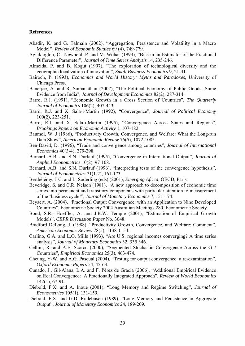
39

References Abadir, K. and G. Talmain (2002), “Aggregation, Persistence and Volatility in a Macro

Model”, Review of Economic Studies 69 (4), 749-779. Agiakloglou, C., Newbold, P. and M. Wohar (1993), “Bias in an Estimator of the Fractional

Difference Parameter”, Journal of Time Series Analysis 14, 235-246. Almeida, P. and B. Kogut (1997), “The exploration of technological diversity and the

geographic localization of innovation”, Small Business Economics 9, 21-31. Bairoch, P. (1993), Economics and World History: Myths and Paradoxes, University of

Chicago Press. Banerjee, A. and R. Somanathan (2007), “The Political Economy of Public Goods: Some

Evidence from India", Journal of Development Economics 82(2), 287-314. Barro, R.J. (1991), “Economic Growth in a Cross Section of Countries”, The Quarterly

Journal of Economics 106(2), 407-443. Barro, R.J. and X. Sala-i-Martin (1992), “Convergence”, Journal of Political Economy

100(2), 223-251. Barro, R.J. and X. Sala-i-Martin (1995), “Convergence Across States and Regions”,

Brookings Papers on Economic Activity 1, 107-182. Baumol, W. J (1986), “Productivity Growth, Convergence, and Welfare: What the Long-run

Data Show”, American Economic Review 76(5), 1072-1085. Ben-David, D. (1996), “Trade and convergence among countries”, Journal of International

Economics 40(3-4), 279-298. Bernard, A.B. and S.N. Durlauf (1995), “Convergence in International Output”, Journal of

Applied Econometrics 10(2), 97-108. Bernard, A.B. and S.N. Durlauf (1996), “Interpreting tests of the convergence hypothesis”,

Journal of Econometrics 71(1-2), 161-173. Berthélémy, J-C. and L. Soderling (eds) (2001), Emerging Africa, OECD, Paris. Beveridge, S. and C.R. Nelson (1981), “A new approach to decomposition of economic time

series into permanent and transitory components with particular attention to measurement of the ‘business cycle’”, Journal of Monetary Economics 7, 151-174.

Beyaert, A. (2004), “Fractional Output Convergence, with an Application to Nine Developed Countries”, Econometric Society 2004 Australian Meetings 280, Econometric Society.

Bond, S.R., Hoeffler, A. and J.R.W. Temple (2001), “Estimation of Empirical Growth Models”, CEPR Discussion Paper No. 3048.

Bradford DeLong, J. (1988), “Productivity Growth, Convergence, and Welfare: Comment”, American Economic Review 78(5), 1138-1154.

Carlino, G.A. and L.O. Mills (1993), “Are U.S. regional incomes converging? A time series analysis”, Journal of Monetary Economics 32, 335 346.

Cellini, R. and A.E. Scorcu (2000), “Segmented Stochastic Convergence Across the G-7 Countries”, Empirical Economics 25(3), 463-474.

Cheung, Y-W. and A.G. Pascual (2004), “Testing for output convergence: a re-examination”, Oxford Economic Papers 54, 45-63.

Cunado, J., Gil-Alana, L.A. and F. Pérez de Gracia (2006), “Additional Empirical Evidence on Real Convergence: A Fractionally Integrated Approach”, Review of World Economics 142(1), 67-91.

Diebold, F.X. and A. Inoue (2001), “Long Memory and Regime Switching”, Journal of Econometrics 105(1), 131-159.

Diebold, F.X. and G.D. Rudebusch (1989), “Long Memory and Persistence in Aggregate Output”, Journal of Monetary Economics 24, 189-209.

40

Durlauf, S.N and P.C.B. Phillips (1988), “Trends versus Random Walks in Time Series Analysis”, Econometrica 56(6), 1333-1354.

Easterly, W. (2002), The Elusive Quest for Growth. Economist's Adventures and Misadventures in the Tropics, MIT Press, Cambridge MA.

Easterly, W. (2003), “The political economy of growth without development: A case study of Pakistan”, in: In Search of Prosperity: Analytic Narratives on Economic Growth edited by Dani Rodrik, Princeton: Princeton University Press.

Ericsson, N.R. and J.R. Halket (2002), “Convergence of output in the G-7 countries”, Mimeo, Division of International Finance, Federal Reserve Board.

Evans, P. (1996), “Using Cross-Country Variances to Evaluate Growth Theories”, Journal of Economic Dynamics and Control 20, 1027–1049.

Fleissig, A.R. and J. Strauss (2001), “Panel unit root tests of OECD stochastic convergence”, Review of International Economics 9, 153-162.

Geweke, J. and S. Porter-Hudak (1983), “The Estimation and Application of Long Memory Time Series Models”, Journal of Time Series Analysis 4(4), 221-238.

Gil-Alana, L.A. (2001), “Seasonal long memory in the aggregate output”, Economics Letters 74(3), 333-337.

Granger, C.W.J. and R. Joyeux (1980), “An Introduction to Long-Memory Time Series Models and Fractional Differencing”, Journal of Time Series Analysis 1(1), 15-29.

Halket, J.R.L. (2005), “Multivariate Fractional Cointegration and GDP Convergence”, Mimeo NYU.

Haubrich, J.G. and A.W. Lo (2001), “The Sources and Nature of Long-Term Memory in Aggregate Output”, Economic Review (Q II), 15-30.

Hoeffler, A. (2002), “The Augmented Solow Model and the African Growth Debate”, Oxford Bulletin of Economics and Statistics 64 (2), 135-158.

Holmes, M.J. (2000), “Convergence in international output: Evidence from panel data unit root tests”, Business Cycle Volatility and Economic Growth Research Paper, No.00-6.

Hosking, J.R.M. (1981), “Fractional Differencing”, Biometrika, 68(1). Hsu, C.-C. (2001), “Change Point Estimation in Regression with I(d) Variables”, Economics

Letters 70, 147-155. Huillery, E. (2009), “History Matters: The Long-Term Impact of Colonial Public Investments

in French West Africa”, American Economic Journal: Applied Economics 1(2), 176-215. Hurvich, C.M. and B.K. Ray (1995), “Estimation of the Memory Parameter for Nonstationary

or Noninvertible Fractionally Integrated processes”, Journal of Time Series Analysis 16, 19-46.

Islam, N. (1995), “Growth Empirics: A Panel Data Approach”, Quarterly Journal of Economics, 1127–1170.

Jensen, M. J. (1999), “Using wavelets to obtain a consistent ordinary least squares estimator of the long-memory parameter”, Journal of Forecasting 18, 17-32.

Johansen, S. (1995), Likelihood-based inference in cointegrated vector auto-regressive models, Oxford University Press.

Journal of Monetary Economics (2003), Carnegie Rochester Conference Series on Public Policy, 50(1), 1-308.

Kabou, A. (1991), Et si l'Afrique refusait le développement?, L’Harmattan, Paris. Kapetanios, G., Shin, Y. and A. Snell (2003), “Testing for a unit root in the nonlinear STAR

framework”, Journal of Econometrics 112, 359-379. Kauffman, S. (1983), “Developmental Constraints: Internal Factors in Evolution”, in B.

Goodwin, N. Holder and C.C. Wylie (eds.), Development and Evolution, CUP, Cambridge.

41

Kim, C.S. and P.C.B. Phillips (2006), “Log Periodogram Regression: The Nonstationary Case”, Cowles Foundation Discussion Paper 1587, Yale University.

Krämer, W. and P. Sibbertsen (2002), “Testing for Structural Change in the Presence of Long Memory”, International Journal of Business and Economics 1(3), 235-243.

Landes, D. (1998), The Wealth and Poverty of Nations. Why Some are so Rich and Some are so Poor, New York: W.W. Norton.

Lau, P.S-H. (1999), “I(0) In, integration and cointegration out: Time series properties of endogenous growth models”, Journal of Econometrics 93(1), 1-24.

Lee, K.L. and M. McAleer (2004), “Convergence and catching up in ASEAN: a comparative analysis”, Applied Economics 36(2), 137-153.

Lee, K., Pesaran, M.H. and R. Smith (1998), “Growth Empirics: A Panel Data Approach—A Comment”, Quarterly Journal of Economics CXIII, 319–323.

Li, Q. and D. Papell (1999), “Convergence of international output: time series evidence for 16 OECD countries”, International Review of Economics and Finance 8(3), 267–280.

Lipsey, R.G., Carlaw, K.I. and C.T. Bekar (2005), Economic Transformations: General Purpose Technologies and Long-term Economic Growth, Oxford: Oxford University Press.

Lucas, R.E. (2002), Lectures on Economic Growth, Harvard University Press. Maddison, A. (2008), Statistics on World Population, GDP and Per Capita GDP, 1-2006 AD,

available online : http://www.ggdc.net/maddison/. Mankiw, N.G., Romer, D. and D.N.Weil (1992), “A Contribution to the Empirics of

Economic Growth”, Quarterly Journal of Economics 107, 407-437. Marmol, F. and C. Velasco (2002), “Trend stationarity versus long-range dependence in time

series analysis”, Journal of Econometrics 108, 25-42. Mayoral, L. (2006), “Further Evidence on the Statistical Properties of Real GNP”, Oxford

Bulletin of Economics and Statistics 68(S1), 901-920. Michelacci, C. and P. Zaffaroni (2000), “(Fractional) Beta Convergence”, Journal of

Monetary Economics 45, 129-153. Nelson, R.R. and S.G. Winter (1982), An evolutionary theory of economic change,

Cambridge, Mass.: Belknap Press of Harvard University Press. Parzen, E. (1981), “Time Series Model Identification and Prediction Variance Horizon”,

Proceedings of Second Tulsa Symposium on Applied Time Series Analysis, Academic Press: New York, 425-447.

Percival, D.B. and A.T. Walden (2000), Wavelet Methods for Time Series Analysis, Cambridge University Press.

Phillips, P.C.B. and D. Sul (2007a), “Some empirics on economic growth under heterogeneous technology”, Journal of Macroeconomics 29(3), 455-469.

Phillips, P.C.B. and D. Sul (2007b), "Transition Modeling and Econometric Convergence Tests”, Econometrica 75(6), 1771-1855.

Robinson, P.M. and D. Marinucci (1997), “Semiparametric frequency-domain analysis of fractional cointegration”, preprint.

Robinson, P.M. and D. Marinucci (2000), “The Averaged Periodogram for Nonstationary Vector Time series”, Statistical Inference for Stochastic Processes 3, 149-160.

Ross, D. and R.E. Friedman (1990), “The Emerging Third Wave: New Economic Development Strategies”, Entrepreneurial Economic Review 90, 3-10.

Shimotsu, K. and P.C.B. Phillips (2000), “Modified Local Whittle Estimation of the Memory Parameter in the Nonstationary Case”, Cowles Foundation Discussion Paper 1265, Yale University.

Shimotsu, K. and P.C.B. Phillips (2005), “Exact local Whittle estimation of fractional integration”, The Annals of Statistics 33(4), 1890-1933.

42

Shimotsu, K. and P.C.B. Phillips (2006), “Local Whittle estimation of fractional integration and some of its variants”, Journal of Econometrics 130, 209-233.

Solow, R.M. (1956), “A Contribution to the Theory of Economic Growth”, Quarterly Journal of Economics 70, 65-94.

Stiglitz, J. (2002), Globalization and Its Discontents, W.W. Norton, New York and London. Strauss, J. (2000), “Is there a permanent component in US real GDP?”, Economics Letters 66,

137-142. Sun, Y., Phillips, P.C.B. and C. Lee (1999), “Efficient Detrending in the Presence of

Fractional Errors”, mimeo, Cowles Foundation, Yale University. Tsangarides, C.G. (2001), “On cross country growth and convergence: Evidence from Africa

and OECD countries”, Journal of African Economies 10(4), 355–389. Velasco, C. (1999), “Non-stationary log-periodogram regression”, Journal of Econometrics

91, 325-371. Verspagen, B. (1995), “Convergence in the global economy. A broad historical viewpoint”,

Structural Change and Economic Dynamics 6(2), 143-165. Wijnberg, N.M. (1996), “Heterochrony, Industrial Evolution and International Trade”,

Journal of Evolutionary Economics 6(1), 99-113.

43

Appendix A. List of countries Central and Latin America Sub-Saharan Africa Asia and Middle East South America Oil-exporting countries New industrialized countries Argentina Angola Hong-Kong Bolivia Cameroon Singapore Brazil Chad South Korea Chile Congo Rep. of Taiwan Colombia Equatorial Guinea China Ecuador Gabon India Paraguay Nigeria Asian Peru Middle-income countries Indonesia Uruguay Botswana Malaysia Venezuela Cape Verde Philippines Central America Lesotho Thailand Costa Rica Mauritius Vietnam El Salvador Namibia Others Guatemala Seychelles Bangladesh Honduras South Africa Burma Nicaragua Swaziland Nepal Panama Low-income countries Sri-Lanka The Caribbean Benin Afghanistan Cuba Burkina Faso Cambodia Dominican Republic Ethiopia and Eritrea Laos Haiti Ghana Mongolia Jamaica Kenya North Korea Puerto-Rico Madagascar Pakistan Trinidad and Tobago Malawi Middle East Mali Bahrain Mozambique Iran Niger Iraq Rwanda Jordan Senegal Kuwait Tanzania Lebanon Uganda Oman Zambia Qatar Fragile countries Yemen Burundi UAE Central African Republic Turkey Comoros S. Arabia Congo Dem. Rep. of Syria The Gambia Guinea Guinea Bissau Liberia Sao Tome Sierra Leone Togo Zimbabwe

Documents

The slow convergence of per capita income between the ...between the developing countries: “growth resistance” and sometimes “growth tragedy” Gilles Dufrénot, Valérie Mignon