The Savings Behavior of Special Purpose Governments: A Panel Study of New York School Districts

The Savings Behavior of Special PurposeGovernments: A Panel Study of New York

School Districts

WILLIAM DUNCOMBE AND YILIN HOU

During the Great Recession, local governments experienced unprecedented fiscalstress. Among localities, special-purpose governments are especially vulnerable torecessions due to their reliance on sole revenue sources. School districts are oneexample that depends heavily on state aid on top of property taxes. However, theliterature is very thin on the savings behavior of special-purpose governments. Thispaper contributes to filling the niche: it uses a 28-year panel of fiscal and socio-economic data for school districts in New York State to examine the determinants offund balances. Ourfindings show that the savings of school districts are affected by theirsize, fiscal capacity, and revenueportfolio. The results are similar for reserved funds andunreserved funds, which suggests that school districts use reserved funds as a savingsmechanism. However, the savings are not necessarily related to economic cycles.

Editor’s Note: As most readers of this journal know, William Duncombe, who was past editor of

Public Budgeting & Finance, died in May 2013. We are pleased to publish this article, with his

former student and co-author, Yilin Hou, posthumously. It was in the review process prior to

Professor Duncombe’s passing, and we thank Professor Hou for the work that he did tomake final

changes and allow us to publish it as a partial tribute to Bill’s long and influential research career.

INTRODUCTION

The Great Recession (December 2007 to June 2009) threw state and local governments into one of

themost severe fiscal crises since theGreat Depression (Smith 2009;McNichol and Lav 2009) and

severely strained the finances of these governments (Boyd and Wachino 2004). Local govern-

ments in particular experienced fiscal problems that were unprecedentedly daunting because of

their thin revenue portfolio and heavy reliance on property tax revenue in a period of declined

William Duncombe is at Center for Policy Research, Syracuse University, Syracuse, New York 13210. He can be

reached at [email protected].

Yilin Hou is at Center for Policy Research, 426 Eggers Hall, Syracuse University, Syracuse, New York 13244. He

can be reached at [email protected].

© 2014 Public Financial Publications, Inc.

Duncombe and Hou / The Savings Behavior of Special Purpose Governments 1

property values. The magnitude of the fiscal challenges facing localities highlights the importance

of understanding their savings behavior and how local fiscal policy affects budget stabilization.

While there is a significant (though still inadequate) literature on the savings behavior of state

governments, the research on local governments has only recently started to accumulate, mostly

since the 2000s. Among localities, special-purpose governments are especially vulnerable to

recessions because these entities serve only one purpose (which is how their name comes) and

rely in most cases on just one revenue source; but the literature is almost non-existent on how

these entities cope with recessions or whether they maintain precautionary savings at all.

School districts are by far the largest type of special purpose governments, collecting 41

percent of all local property taxes and representing 37 percent of total local government

expenditure in FY2009 (U.S. Census Bureau 2011a, 2011b). They cover the whole country, serve

all households, and affect the finances of property owners and renters one way or another with

their heavy dependence on property tax revenues. Since the late 1970s, states have been

increasingly more involved in education financing for the purpose of achieving equity. As of the

1990s, close to half of school budgets on average come from their state and thus, school districts

have become reliant also on state aid. This is why the decline of property values during the Great

Recession hit school districts so hard (Davis 2008), on top of state aid reductions amidst squeezed

state budgets. However, the literature is very thin on the savings behavior of school districts.

The objective of this paper is to contribute to the literature on the savings behavior of school

districts by examining their fund balances. This study employs a 28-year panel of school districts

in New York State. New York represents a particularly good setting for examining school district

savings because the state has imposed relatively few fiscal constraints on the fiscal behavior of

school districts, and the state’s funding for education is relatively more decentralized than inmany

other states. The rest of the paper is organized into four sections. The next section discusses

previous research on state and local government savings behavior. Section three presents the

empirical model and data used in the analysis. Section four presents and discusses empirical

results. Section five concludes with a discussion of implications of the findings and directions for

future research.

PREVIOUS RESEARCH

There is a growing body of literature over the last decade looking at savings behavior of state and

local governments. Research has focused on three broad questions: (1) what constitutes

government savings or slack resources; (2) what factors are related to the accumulation of

“slack”; and (3) whether the existence of fund balances or budget stabilization funds actually

stabilized subnational budgets. The first two are relevant for this paper.

With regard to the first question, research has tended to focus on unreserved (undesignated)

general fund balances (UB)1 or budget stabilization funds (BSF) at the state level

1. The last year of data we used for analysis was FY2009, whichwas before the implementation of GASB 54. Thus,

the new classification of fund balances as nonspendable, restricted, committed, assigned, and unassigned fund

balances did not apply.

2 Public Budgeting & Finance / Fall 2014

(Hou 2003, 2004). One of the questions addressed by several studies is whether BSF and UB act

as substitutes or complements (Hou andDuncombe 2008).While a few states do allow their local

governments to create local BSF (Gianakis and Snow 2007), for most localities fund balances,

particularly from the general fund, represent their primary source of savings. Hendrick (2006)

and Marlowe (2005) point out that local governments may have several indirect sources of

savings including reserve funds, reductions in pay-as-you-go financing of capital, and interfund

transfers from enterprise funds. For special district governments, typically only fund balances

are readily available as savings. We will focus in this paper on general fund balances—both

unreserved and reserved balances.

Some scholars highlight the theoretical differences in why organizations might accumulate

slack resources. From a public choice perspective, slack resources allow bureaucrats to extract

rents in the form of higher compensation and to distribute slack resources in order to maintain

coalitions (Wintrobe 1997). Thus, we might expect that governments with strong public

employee unions or relatively weak incentives for voters tomonitor the efficiency of government

operations might be more apt to accumulate slack. Some research on New York school districts

show that local fiscal capacity, voter education level, the tax price of local public services, and

state aid may be related to school district inefficiency (Duncombe, Miner, and Ruggerio 1997;

Duncombe and Yinger 1997).

Hendrick (2006) emphasizes that organizations use slacks as buffer against adverse shocks

and thus the amount of slack is correlated to the extent of risk, uncertainty, and instability

organizations face. For this study, we might expect that small school districts with unstable

enrollments, unstable property values, high debt burdens, and heavy reliance on state aid or sales

taxes to be more apt to accumulate debt. Another view is that local governments are generally

risk averse and will accumulate as much slack as is feasible, given their political and economic

constraints. Under this view, local governments in the most challenging fiscal environments will

be the least able to accumulate sizeable fund balances. Thus, fund balances reflect the underlying

fiscal health of localities.

However, empirical results from previous research on local government savings

(Marlowe 2005; Gianakis and Snow 2007; Hendrick 2006; and Wang and Hou 2012) provide

a mixed picture that does not fully support any of the above explanations, which means there is a

huge niche to fill. Inconclusive as prior research is, two findings from these studies are useful

directions: that governments of small jurisdictions (in terms of population) or those less

dependent on state aid (in terms of aid ratio) tend to accumulate higher fund balances. This

research builds on these for exploration into the savings behavior of school districts.

EMPIRICAL MODELS AND DATA SOURCES

Modeling Fund Balances

The literature on government savings behavior and fiscal health has highlighted several types of

factors, which might be related to the level of local government savings. In selecting factors


associated with fund balances, it is important to identify which factors are under the control of

the government and which are external factors outside government control. Given the unique

features of school districts as a sole service provider, we tailor the model of fund balances to

reflect the aspects of service delivery and revenue sources as associated with special-purpose

governments. Drawing from the literature on the demand for and costs of providing education

services (e.g., Ladd and Yinger 1994; Duncombe and Yinger 2000) as well as the research on

state and local government savings discussed earlier, we propose a simple but straightforward

model to identify the determinants of fund balances for school districts. The model is: FB¼ ƒ (R,

D, C, I). Specifically, general fund balances (FB) are affected by: (1) revenue related variables

(R); (2) factors related to the demand for public education (D); (3) variables related to the cost of

providing educational services (C); and (4) state institutional constraints (I) that include

management stability at the district level. We explain these as follows.

Fund balances. We choose the total, unreserved, and reserved balances of the general fund as a

percent of operating expenditures as our indicators of school district savings, because total

balance is an aggregate of fiscal condition. Unreserved fund balance is the most readily available

resource once the need arises to cope with a revenue shock and reserved balance can also be of

much use in the case of emergencies. The denominator of the balance ratios is the sum of

expenditures on personnel, employee benefits, and external contracts. This choice of ours differs

from analyses of state government savings in previous studies (e.g., Hou 2003, 2005) that focus

on the unreserved undesignated balances (UUB), because New York State imposes constraints

over the size of UUB that school districts are allowed to accumulate.2 Even though unreserved

funds are fungible in comparison to UUB, New York school districts may accumulate resources

here to buffer against fiscal shocks.

Revenue and debt measures. Theory on the savings behavior of state governments suggests that

the revenue structure and debt burdens can affect the level of savings (Hou 2003). School

districts with more diverse local revenue sources may be less vulnerable to shocks that mainly

affect one of these sources. For example, the decline in housing prices during the Great

Recession exerted a large negative effect on property tax revenues; but access to a local sales tax

and fees/charges might reduce the adverse effects from decreases in property tax revenue.

On the other hand, property taxes are a relatively more stable source of revenue, compared

to sales and income taxes.3 We measure revenue diversification as the share of district

2. NewYork State Consolidated Laws, Ch. 56 Real Property Tax, Article 13 Special Provisions Relating to School

Districts, Section 1318-1: “…the amount of unexpended surplus funds…ha[s] been applied in determining the

amount of the school tax levy. Surplus funds…shall mean any operating funds in excess of two percent of the current

school year budget, and shall not include funds properly retained under other sections of this law.” Recently, this law

was changed so that in academic year 2008–09 and thereafter, the maximum ceiling is 4 percent.

3. The local sales tax in New York State is administered at the county level. Counties can choose to share some of

their sales tax revenue with school districts; but not all counties do. Thus, some school districts have access to sales

tax revenue while others do not.


own-source revenue from property taxes. The lower this ratio, the more diversified is the

revenue composition.

The ability of school districts to raise property taxes for coping with revenue shortfalls

depends on how high their effective property tax rates already are. Districts with high rates have

limited ability to tax their way out of a budget crisis. Heavy dependence on state aid could also

make a district vulnerable to large decreases in intergovernmental aid during a recession. We

measure aid dependence as the share of total revenue from state and federal aid. We also include

the level of state aid (per pupil) in the models. One of the long-term commitments that school

districts make is to invest in capital facilities that are financed with debt. Districts with high debt

burdens will bemore constrained in their ability to cope with budget deficits through expenditure

reductions since debt service levels are pre-set at bond issuance. To measure debt burden, we use

long-term debt outstanding as percent of total property values.

Demand factors. Research on the demand for local government services has focused primarily

on the impact of local fiscal capacity and tax prices on the demand. In the context of government

savings behavior, high fiscal capacity makes it easier for districts to maintain high fund balances

and is less an incentive for voters to monitor the operational efficiency of their schools. Local

fiscal capacity is commonly measured with either property values or income. We expect that

both the level and the growth rate of tax capacity affect the fiscal health of school districts.While

property values more closely reflect the major local tax base, ultimately all taxes on residents

have to be paid out of their income. Thus, residents who are property wealthy but income poor

(e.g., senior/retiree households) may be hesitant to support property tax increases. We use three

measures of district fiscal capacity—per pupil gross income, property value growth, and the ratio

of estimated full market value of property to income.

High tax prices imply that local voters bear a higher burden for funding local services, which

increases their incentive tomonitor government efficiency. The commonmeasure of tax prices is

tax share—the ratio of median residential property values over per pupil total property values.

NewYork introduced in the late 1990s a “homestead exemption” for school property taxes that is

funded by the state under the “School Tax Relief” (STAR) program. STAR lowers the tax price

to local voters in financing education with property taxes (Eom, Duncombe, and Yinger 2011).

Variation in the STAR tax share across districts potentially affects the savings behavior of local

governments as well.4

Cost factors. Factors outside a district’s control include geographic differences in salary (and

other key resources), the proportion of disadvantaged students, and enrollment (Duncombe and

Yinger 2008). We measure geographic wage variation using average monthly compensation for

private sector fulltime employees at the county level. Students living in poverty often face

greater difficulty making academic achievements in school. Unfortunately, the student poverty

measure (students receiving subsidized lunch) is available only since 1987. As a compromised

4. The STAR tax price for the decisive voter in a school district can be measured as [1� (STAR exemption)/

median residential property value] (Eom, Duncombe, and Yinger 2011). The amount of exemptions vary by the

income of households and region of the state.


remedy, we impute the share of students in poverty for years 1982 through 1986.5 Costs may also

be affected by economies of scale and enrollment volatility. To capture economies of scale, we

include enrollment and enrollment squared. Enrollment volatility is measured as the average

variation around a regression trend line.6 The most common indicator of economic activity is

unemployment rate, which would ideally be at the school district level, but the county is the

lowest geographic level for annual reporting. Thus, county level data are the best we can use.

Management changes and institutional constraints. Studies of the determinants of savings

include variables of government form or management changes. New York school districts (with

the exception of the large cities), have only one form of government—an elected Board of

Education and an appointed superintendent. To capture the influence of management changes on

fund balances, we include superintendent turnover in the previous two years.7 Studies of state

and local savings behavior also look at whether institutional constraints (like balanced budget

requirements and tax and expenditure limitations) affect fund balances. New York school

districts face a constraint on borrowing which is limited by state statute. We use the debt limit

ratio to the market value of property to assess the effect of the constraint on savings.

Data Sources

Our units of analyses are school districts serving students from kindergarten to the 12th grade.

Our sample period is 1982–2009 (FY1981–82 to FY2008–09) that covers three periods of

economic expansion (1983–89, 1992–2000, and 2002–08) and contraction (1982, 1990–91,

2001, 2008–09).8 The sample includes 600 out of 670 total school districts in New York State.9

The New York State Education Department (NYSED) is the other major source of information.

NYSED collects information on enrollment, the number of students in different need categories,

district personnel by type, teacher salary, teacher experience and education, measures of state aid

5. The share of students receiving subsidized lunch are regressed on the share of African American students, per

pupil income, the share of personal income in the county from transfer payments, andwhether the district is classified

as “high need” by the New York State Education Department (adjusted R2¼ 0.7). The predicted value is used to

impute values in years with missing data.

6.We regress enrollment on time for the previous five years. The stability measure is the standard error of estimate

divided by the average enrollment over this five-year period.

7. The variable can take on values of 0, 0.5 (if 1 turnover), or 1 (if 2 turnovers). We also looked at using a simple

dummy variable if there was any turnover in the previous two years or three years; the results were similar.

8. These are only approximations of the economic cycle. The official business cycles established by NBER

Business Cycle Dating Committee based on real GDP growth rates include recessions from the 3rd quarter of 1981 to

the 4th quarter of 1982, the 3rd quarter of 1990 to the 1st quarter of 1991, the 1st quarter of 2001 to the 4th quarter of

2001, and December 2007 to June of 2009. Cyclical patterns can vary across states and for other economic indicators

(e.g., employment and personal income).

9. NewYork City was excluded because it is an outlier in terms of size (25 times the size of the next largest district,

Buffalo) and comparable financial data were not available for many years. We excluded school districts serving only

a subset of grades (e.g., K6, K8, and high school districts) or students, because these districts may face different fiscal

policies and environments than K12 districts serving students of all grades.


by aid program, and expenditures. Adjusted gross income (AGI) estimates are provided by the

New York Office of Taxation and Finance (NYOTF) to NYSED. Financial information used in

our analyses is collected from unaudited annual financial statements that school districts submit

each year to NYSED (labeled as the “ST3 reports”).10 Data thereof is summarized and published

by the New York State Office of the Comptroller (NYSOC) in a local government financial

database that also includes enrollments and estimates of the market value of property in each

school district. County unemployment data was provided by the New York State Department of

Labor. All financial data used in this study is adjusted for inflation using the GDP deflator (in

year 2000 dollars). Descriptive statistics are in Table 1.

DESCRIPTIVE ANALYSES AND EMPIRICAL RESULTS

In this section we first provide a descriptive picture of school district fund balances, then estimate

different models to determine which factors seem to be most related to changes in school district

fund balances.

Descriptive Analyses

Before conducting regression analysis, some descriptive analysis of the data helps us examine

patterns for both the total, the unreserved, and the reserved fund balances to answer two

questions: (1) what are the overall trends in fund balances of New York school districts and

how the trends move with the economic cycles; and (2) are there significant differences in

fund balances and in their patterns across types of school districts? Figure 1 illustrates fund

balance ratios during the last three decades. Total general fund balances on average show a

steady increase, particularly since FY2000. While there is some volatility in this measure

around recessionary periods, there were no significant drops in balance ratios during

recessions. In contrast, the ratios of unreserved fund balance (UB) and unreserved

undesignated fund balance (UUB) remained roughly flat throughout the sample period till a

tip appeared in 2007–09, in tandem with total fund balance. These trends imply that school

districts on average added significantly in the most recent 15 years to their general fund

balances, but the relative size of the unreserved fund balances did not increase until the Great

Recession. The rise of UB and UUB during the Great Recession deserves special attention; we

will revisit this point later.

To determine whether average fund balances are masking variation among types of districts,

we place school districts into different categories by their need and resource capacity. Here

“need” refers to ratios of students in a district receiving subsidized lunch and “resource capacity”

10. Districts are also required to submit audited financial statements to the State Education Department. While the

audited reports are presumably more accurate than the unaudited ones, they are less detailed and are not available in

electronic form. NYSED and the NYOSC have checked the accuracy of the ST3 reports and found they fairly

reflected audited accurate information.


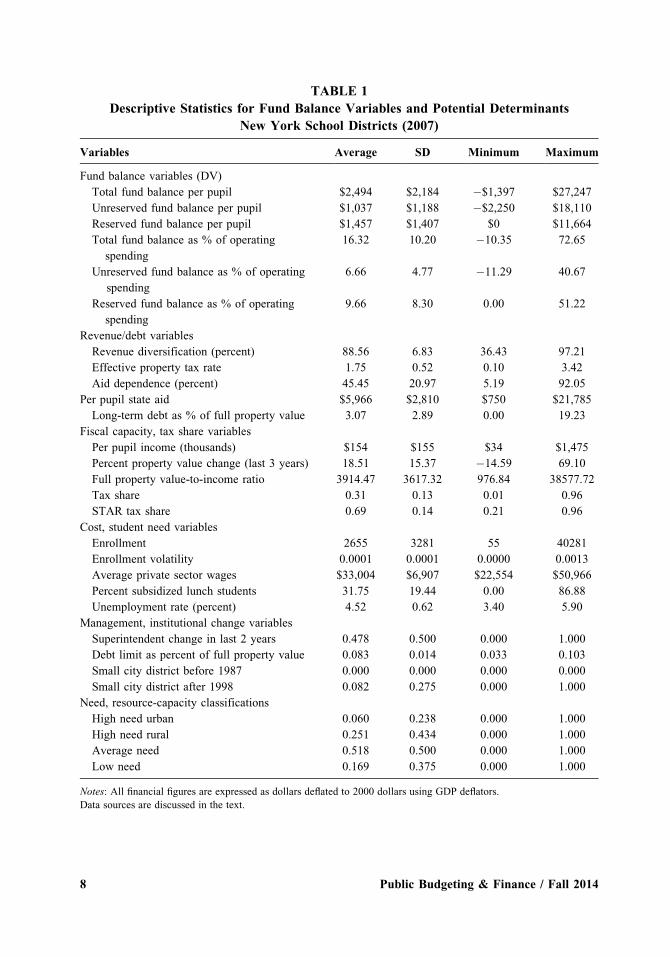
TABLE 1

Descriptive Statistics for Fund Balance Variables and Potential Determinants

New York School Districts (2007)

Variables Average SD Minimum Maximum

Fund balance variables (DV)

Total fund balance per pupil $2,494 $2,184 �$1,397 $27,247

Unreserved fund balance per pupil $1,037 $1,188 �$2,250 $18,110

Reserved fund balance per pupil $1,457 $1,407 $0 $11,664

Total fund balance as % of operating

spending

16.32 10.20 �10.35 72.65

Unreserved fund balance as % of operating

spending

6.66 4.77 �11.29 40.67

Reserved fund balance as % of operating

spending

9.66 8.30 0.00 51.22

Revenue/debt variables

Revenue diversification (percent) 88.56 6.83 36.43 97.21

Effective property tax rate 1.75 0.52 0.10 3.42

Aid dependence (percent) 45.45 20.97 5.19 92.05

Per pupil state aid $5,966 $2,810 $750 $21,785

Long-term debt as % of full property value 3.07 2.89 0.00 19.23

Fiscal capacity, tax share variables

Per pupil income (thousands) $154 $155 $34 $1,475

Percent property value change (last 3 years) 18.51 15.37 �14.59 69.10

Full property value-to-income ratio 3914.47 3617.32 976.84 38577.72

Tax share 0.31 0.13 0.01 0.96

STAR tax share 0.69 0.14 0.21 0.96

Cost, student need variables

Enrollment 2655 3281 55 40281

Enrollment volatility 0.0001 0.0001 0.0000 0.0013

Average private sector wages $33,004 $6,907 $22,554 $50,966

Percent subsidized lunch students 31.75 19.44 0.00 86.88

Unemployment rate (percent) 4.52 0.62 3.40 5.90

Management, institutional change variables

Superintendent change in last 2 years 0.478 0.500 0.000 1.000

Debt limit as percent of full property value 0.083 0.014 0.033 0.103

Small city district before 1987 0.000 0.000 0.000 0.000

Small city district after 1998 0.082 0.275 0.000 1.000

Need, resource-capacity classifications

High need urban 0.060 0.238 0.000 1.000

High need rural 0.251 0.434 0.000 1.000

Average need 0.518 0.500 0.000 1.000

Low need 0.169 0.375 0.000 1.000

Notes: All financial figures are expressed as dollars deflated to 2000 dollars using GDP deflators.

Data sources are discussed in the text.


refers to property wealth and income.11 Districts with relative high needs and low fiscal capacity

are identified as “high-need” districts. In contrast, districts with low needs and high resource

capacity are identified as “low-need” districts. If fund balance ratios simply reflected underlying

condition of the local economy, we would expect that high-need districts have low fund balances

and low-need districts have high balances. On the other hand, if districts consciously managed

their balances to minimize budget shocks, we might expect that there will either be little

difference in fund balance by type of district or that high-need districts might actually have

higher balances going into a recession. Table 2 reports fund balances by the several periods of the

economic cycles and by the district categories. It appears that the fund balances, at least on

average, are not very cyclically sensitive, echoing the patterns in Figure 1. While some ratios are

slightly lower during recessions than during expansions, the differences are not large or vary

much by the boom-bust cycle. The variation in fund balances is much lower than for overall

economic measures such as unemployment and income. One exception is large cities, whose

fund balances did drop significantly during the 2001–02 recession. The lack of a cyclical pattern

in fund balances for most school districts is in striking contrast to the experience of state

governments (Hou 2003).

FIGURE 1

Fund Balances as a Percent of Operating Expenditures

New York School Districts 1981–2009

0

5

10

15

20

25Fu

nd B

alan

ce a

s Per

cent

of E

xpen

ditu

res

Total fund balanceUnreserved Fund BalanceUnres. Undesignated Fund Balance

19811983

1985198719891991199319951997199920012003200520072009

11. NYSED’s “Need-to-Resource-Capacity Index” is calculated as the ratio of a standardized measure of student

poverty and resource capacity (average of income and property wealth indexes). The numerator is measured using a

weighted average of the two-year average of the subsidized lunch rate for 2001 and 2002 and the 2000 Census child

poverty rate. The denominator is a fiscal capacity measure used by New York called the combined wealth ratio

(CWR), which is an average of an income index and property wealth index (centered around the state average) and

was measured for 2001 (NYSED 2010).


To look more closely at the fund balances, we categorize the reserved funds into four groups

by purpose (NYSED 2011) as related to: (1) insurance and fringe benefits, (2) capital and debt,

(3) tax certiorari or tax reduction, and (4) encumbrances and inventories, respectively.12 Details

are shown in Figure 2. Because over the last several decades New York changed the reserve

funds that school districts can use, the patterns presented should be viewed only as suggestive.

The largest change in reserve fund classification occurred in FY2001. Most of the new funds

were in the insurance and fringe benefits category. One of the reserves for “employee benefit

accrued liability” was first funded in FY2005 and by FY2009 represented 29 percent of total

TABLE 2

Fund Balance Ratios by Phase of Business Cycles By District

Need/Resource Capacity Type

Business cycle

All

districts

Large

cities

(without NYC)

Other high

need urban

High

need rural

Average

need

Low

need

Total fund balance

Recession (1982–83) 9.0 1.0 6.6 9.5 8.5 10.2

Expansion (1984–89) 9.4 4.9 7.0 11.0 8.5 10.0

Recession (1990–91) 9.5 8.2 7.0 9.8 8.8 11.2

Expansion (1992–2000) 10.7 6.6 6.6 11.8 9.8 11.7

Recession (2001–02) 12.1 2.5 8.0 14.3 10.9 11.8

Expansion (2003–07) 15.0 6.3 10.7 17.6 15.0 15.0

Recession (2008–09) 19.9 11.0 15.5 24.6 21.3 18.7

Average recessions 12.6 5.7 9.3 14.6 12.4 13.0

Average expansions 11.4 6.0 7.8 13.0 10.7 12.0

Unreserved fund balances

Recession (1982–83) 7.5 0.1 5.2 8.2 7.0 8.4

Expansion (1984–89) 7.6 3.9 5.1 9.2 6.8 7.8

Recession (1990–91) 7.6 6.7 4.9 7.9 7.2 8.5

Expansion (1992–000) 7.6 4.2 4.5 8.9 7.1 7.1

Recession (2001–02) 6.9 1.3 4.0 8.5 6.1 6.0

Expansion (2003–07) 7.0 2.8 4.6 8.6 6.5 6.4

Recession (2008–09) 8.6 8.2 8.0 11.4 8.5 7.5

Average recessions 7.6 4.1 5.5 9.0 7.2 7.6

Average expansions 7.5 3.8 4.7 8.9 6.9 7.2

Note: Because the data is annual we can only approximate the business cycles.

12. These four categories are reserves for: (1) Unemployment Insurance, Worker’s Compensation, insurance

reserves, liability losses, insurance recoveries, and retirement systems credits; (2) capital, repairs, debt service, and

property losses; (3) tax certiorari, tax reduction and taxes raised outside tax limit (applies only to five largest cities);

and (4) miscellaneous. Data are available only from 1991.


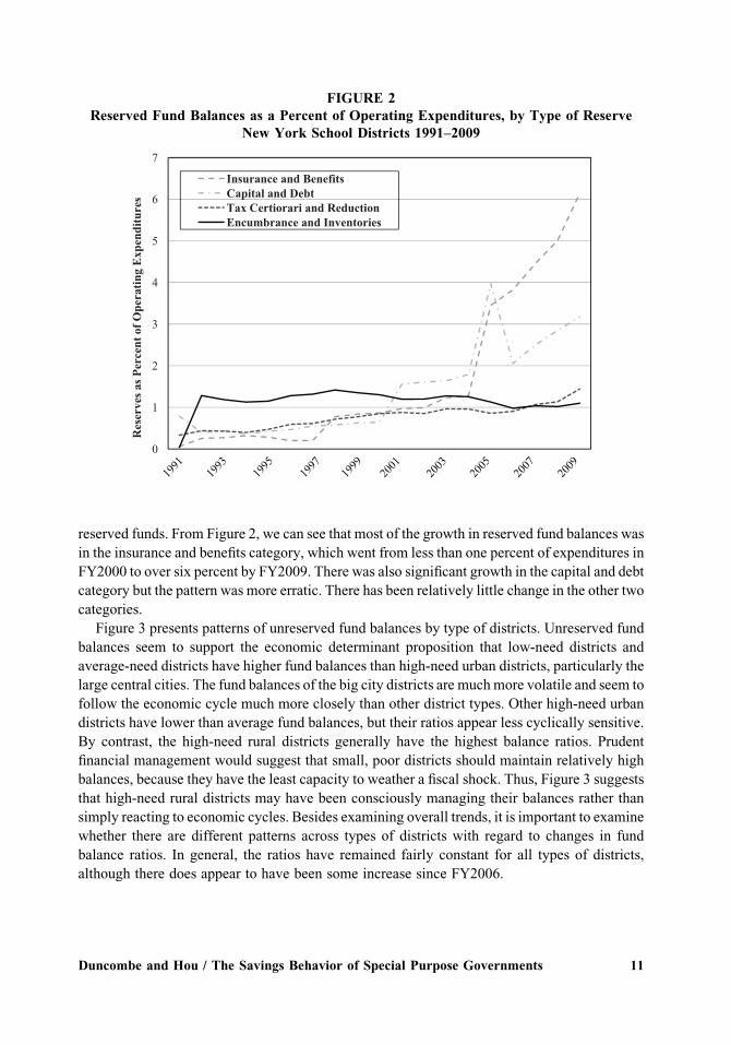
reserved funds. From Figure 2, we can see that most of the growth in reserved fund balances was

in the insurance and benefits category, which went from less than one percent of expenditures in

FY2000 to over six percent by FY2009. There was also significant growth in the capital and debt

category but the pattern was more erratic. There has been relatively little change in the other two

categories.

Figure 3 presents patterns of unreserved fund balances by type of districts. Unreserved fund

balances seem to support the economic determinant proposition that low-need districts and

average-need districts have higher fund balances than high-need urban districts, particularly the

large central cities. The fund balances of the big city districts are muchmore volatile and seem to

follow the economic cycle much more closely than other district types. Other high-need urban

districts have lower than average fund balances, but their ratios appear less cyclically sensitive.

By contrast, the high-need rural districts generally have the highest balance ratios. Prudent

financial management would suggest that small, poor districts should maintain relatively high

balances, because they have the least capacity to weather a fiscal shock. Thus, Figure 3 suggests

that high-need rural districts may have been consciously managing their balances rather than

simply reacting to economic cycles. Besides examining overall trends, it is important to examine

whether there are different patterns across types of districts with regard to changes in fund

balance ratios. In general, the ratios have remained fairly constant for all types of districts,

although there does appear to have been some increase since FY2006.

FIGURE 2

Reserved Fund Balances as a Percent of Operating Expenditures, by Type of Reserve

New York School Districts 1991–2009

0

1

2

3

4

5

6

7

Res

erve

s as P

erce

nt o

f Ope

ratin

g E

xpen

ditu

res

Insurance and BenefitsCapital and DebtTax Certiorari and ReductionEncumbrance and Inventories

1991

1993

1995

1997

1999

2001

2003

2005

2007

2009


The pattern for reserved fund ratios by need/resource capacity category (Fig. 4) is even more

distinct. Low-need, average-need, and high-need rural districts all show rapid growth in reserved

fund ratios from under two percent in the early 1980s to over 11 percent by FY2009. For low-

need districts, significant growth occurred in both of the last two decades while for average-need

and high-need rural districts, most of the growth was since 1997. Reserved funds in the other

high-need districts also experienced significant growth although the pattern was more volatile.

By contrast, there was little growth in the reserved fund balance ratio for big cities and their ratios

were volatile and generally procyclical.

Empirical Methodology

The regression models estimated in this paper are based on panel data. The advantage of using

panel data is to make it easier to identify the relationship between variables by capturing how

they move together over time. To assure that explanatory variables precede the dependent

variable, we use one-year lags for most variables. We also experimented with two-year lags and

three-year moving averages and the results were similar.

Panel data offers some other advantages but also presents some methodological challenges.

The major methodological challenge in research on government fiscal decisions is to develop

accurate estimates of the relationships between fiscal variables. Often fiscal variables are set as

part of the annual budgeting process, whichmakes it difficult to isolate the direction of the causal

FIGURE 3

Unreserved Fund Balance as a Percent of Operating Expenditures By

Need/Resource Capacity Categories 1981–2009

-4

-2

0

2

4

6

8

10

12

14Fu

nd B

alan

ce a

s Per

cent

of E

xpen

ditu

res

High Need RuralLow NeedAverage NeedOther High Need UrbanBig Cities


relationship—what is commonly called a potential endogeneity bias. In our models, potentially

endogenous variables include measures of revenue diversification, aid dependence, effective

property tax rate, and debt burden. The common approach to treating endogeneity is to identify

one or more exogenous variables (instruments) that are strongly correlated with the endogenous

variables but do not have an independent relationship with the dependent variable. One method

for selecting instruments is to use lagged values of the endogenous variables expressed in the

form of ranks (Kroszner and Stratmann 2000). We use two-year and three-year lags of each

endogenous variable. Ranks are created by dividing the distribution of the lagged endogenous

variable into thirds and assigning the lowest third a value of “1,” the middle third “2,” and the

upper third “3.” These ranks should be strongly related to the endogenous variables but should be

uncorrelated with the error term, except for observations close to the cross-over points. With

only two cross-over points, this problem should be minimized. We used a couple of weak

instrument tests to identify whether the instruments are strongly correlated with the endogenous

variables and we also used an over-identification test to see whether the instruments are

exogenous (Wooldridge 2003).13

FIGURE 4

Reserved Fund Balance as a Percent of Operating Expenditures By

Need/Resource Capacity Categories 1981–2009

0

2

4

6

8

10

12

14Fu

nd B

alan

ce a

s Per

cent

of E

xpen

ditu

res

Big CitiesOther High Need UrbanHigh Need RuralAverage NeedLow Need

19811983

1985198719891991199319951997199920012003200520072009

13. We examined two weak instrument tests. First, partial F-statistics from the first-stage regressions were

calculated. The typical rule of thumb is that theseF-statistics need to be above 10 for the instruments to be acceptable

(Staiger and Stock 1997). A second weak instrument test (Baum, Schaffer, and Stillman 2007) involves comparing

the Kleibergen-Paap rk Wald statistic to critical values established by Stock and Yogo (2005).


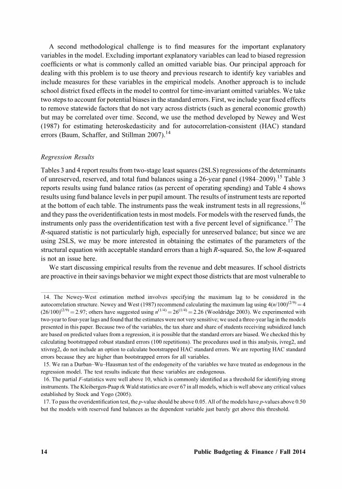
A second methodological challenge is to find measures for the important explanatory

variables in the model. Excluding important explanatory variables can lead to biased regression

coefficients or what is commonly called an omitted variable bias. Our principal approach for

dealing with this problem is to use theory and previous research to identify key variables and

include measures for these variables in the empirical models. Another approach is to include

school district fixed effects in the model to control for time-invariant omitted variables. We take

two steps to account for potential biases in the standard errors. First, we include year fixed effects

to remove statewide factors that do not vary across districts (such as general economic growth)

but may be correlated over time. Second, we use the method developed by Newey and West

(1987) for estimating heteroskedasticity and for autocorrelation-consistent (HAC) standard

errors (Baum, Schaffer, and Stillman 2007).14

Regression Results

Tables 3 and 4 report results from two-stage least squares (2SLS) regressions of the determinants

of unreserved, reserved, and total fund balances using a 26-year panel (1984–2009).15 Table 3

reports results using fund balance ratios (as percent of operating spending) and Table 4 shows

results using fund balance levels in per pupil amount. The results of instrument tests are reported

at the bottom of each table. The instruments pass the weak instrument tests in all regressions,16

and they pass the overidentification tests in most models. For models with the reserved funds, the

instruments only pass the overidentification test with a five percent level of significance.17 The

R-squared statistic is not particularly high, especially for unreserved balance; but since we are

using 2SLS, we may be more interested in obtaining the estimates of the parameters of the

structural equation with acceptable standard errors than a high R-squared. So, the low R-squared

is not an issue here.

We start discussing empirical results from the revenue and debt measures. If school districts

are proactive in their savings behavior wemight expect those districts that are most vulnerable to

14. The Newey-West estimation method involves specifying the maximum lag to be considered in the

autocorrelation structure. Newey and West (1987) recommend calculating the maximum lag using 4(n/100)(2/9)¼ 4

(26/100)(2/9)¼ 2.97; others have suggested using n(1/4)¼ 26(1/4)¼ 2.26 (Wooldridge 2003). We experimented with

two-year to four-year lags and found that the estimates were not very sensitive; we used a three-year lag in themodels

presented in this paper. Because two of the variables, the tax share and share of students receiving subsidized lunch

are based on predicted values from a regression, it is possible that the standard errors are biased. We checked this by

calculating bootstrapped robust standard errors (100 repetitions). The procedures used in this analysis, ivreg2, and

xtivreg2, do not include an option to calculate bootstrapped HAC standard errors. We are reporting HAC standard

errors because they are higher than bootstrapped errors for all variables.

15. We ran a Durban–Wu–Hausman test of the endogeneity of the variables we have treated as endogenous in the

regression model. The test results indicate that these variables are endogenous.

16. The partial F-statistics were well above 10, which is commonly identified as a threshold for identifying strong

instruments. The Kleibergen-Paap rkWald statistics are over 67 in all models, which is well above any critical values

established by Stock and Yogo (2005).

17. To pass the overidentification test, the p-value should be above 0.05. All of the models have p-values above 0.50

but the models with reserved fund balances as the dependent variable just barely get above this threshold.


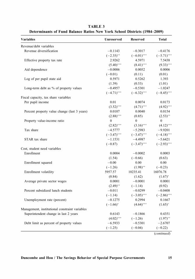
TABLE 3

Determinants of Fund Balance Ratios New York School Districts (1984–2009)

Variables Unreserved Reserved Total


Revenue diversification �0.1143

(�2.35)��0.3017

(�6.01)��0.4176

(�5.71)��

Effective property tax rate 2.9262

(5.40)��4.5971

(8.41)��7.5438

(9.33)��

Aid dependence �0.0006

(�0.01)

0.0052

(0.11)

0.0006

(0.01)

Log of per pupil state aid 0.5971

(1.39)

0.5262

(0.53)

1.393

(1.01)

Long-term debt as % of property values �0.4957

(�4.71)��0.5301

(�6.32)��1.0247

(�8.45)��


Per pupil income 0.01

(3.52)��0.0074

(4.71)��0.0173

(4.92)��

Percent property value change (last 3 years) 0.0107

(2.88)��0.0040

(0.85)

0.0154

(2.53)��

Property value-income ratio 0

(2.82)��0

(3.16)��0

(4.12)��

Tax share �4.5777

(�3.47)��5.2983

(�3.47)��9.9201

(�4.18)��

STAR tax share �1.1531

(�0.87)

�4.4987

(�3.47)��5.6421

(�2.93)��


Enrollment 0.0004

(1.54)

�0.0002

(�0.66)

0.0003

(0.63)

Enrollment squared �0.00

(�1.26)

0.00

(1.98)��0.00

(�0.23)

Enrollment volatility 5957.57

(0.84)

10235.41

(1.62)

16076.78

(1.67)�

Average private sector wages 0.0001

(2.49)��0.0001

(�1.14)

0.0001

(0.92)

Percent subsidized lunch students �0.011

(�1.14)

�0.0299

(�3.05)��0.0408

(�2.86)��

Unemployment rate (percent) �0.1275

(�1.66)�0.2994

(4.64)��0.1667

(1.65)�

Management, institutional constraint variables

Superintendent change in last 2 years 0.6143

(4.02)��0.1866

(�1.26)

0.4351

(1.97)��

Debt limit as percent of property values �6.5933

(�1.25)

�0.5301

(�0.04)

�2.6707

(�0.22)

(continued)


fiscal shocks to accumulate larger fund balances. For example, with regard to revenue and

debt, school districts that have lower local revenue diversity, that have higher property tax

rates, that are more dependent on state and federal aid, that have relatively low levels of

per pupil state aid, and that have higher debt burdens would possess higher ratios of fund

balances. The results are not all as expected; coefficients of these variables display a mixed

picture. On the one hand, districts with lower revenue diversification and higher property tax

rates do tend to have higher fund balance ratios, as expected. On the other hand, districts that are

more dependent on state and federal aid, that have higher per pupil state aid, and that have

higher debt burdens tend to have lower relative fund balance ratios—these results are not what

we expect. Though only the measures of revenue diversification, effective tax rates, and debt

burdens are statistically significant in most models, the results are overall consistent across

models.

Turning to the demand variables, we might expect that districts with lower income and lower

growth in property wealth would accumulate more fund balances since it will be more difficult

for them to raise local revenue if there is a fiscal shock. Instead, what we find is that districts with

higher income and more rapid growth in property values accumulate larger relative fund

balances, against expectations. Counter intuitive as these results may be, they reveal some

unique fiscal behavior of special-purpose governments that are different from general purpose

governments. Our hypotheses are built on existing literature that is exclusively drawn on general

TABLE 3 (Continued)


Small city district before 1987 0.5451

(1.35)

0.6291

(1.67)�1.2065

(2.11)��

Small city district after 1997 0.791

(2.67)��2.261

(�6.61)��1.481

(�3.15)��

Sample size 15,367 15,367 15,367

Centered R-square 0.03 0.22 0.36

Weak instrument test

F-statistic (revenue diversification) 243.38 243.38 243.38

F-statistic (effective property tax rate) 115.12 115.12 115.12

F-statistic (aid dependence) 255.42 255.42 255.42

F-statistic (Long-term debt as% of property values) 215.16 215.16 215.16

Kleibergen-Paap rk Wald F statistic 67.73 67.73 67.73

Overidentification test (p-value) 0.28 0.05 0.12

Notes: (1) t-Statistics are in parentheses. (2) Dependent variable is the specified general fund balance as percent of

operating spending. (3) All explanatory variables are lagged one year unless indicated otherwise. (4) All models include year

fixed effects and school district fixed effects. (5) Models are estimated with a linear two-step general method of moments

(GMM) estimator. (6) Endogenous variables are revenue diversification, effective tax rate, aid dependence, and total

outstanding debt as a percent of property values. Instruments for the endogenous variables are explained in the text.

(7) Hypothesis tests are based on the Newey andWest (1987) method for estimating heteroskedasticity and autocorrelation-

consistent (HAC) standard errors. (8) Asterisks denote statistical significance at the 1% (��), 5% (��), and 10% (�)levels.


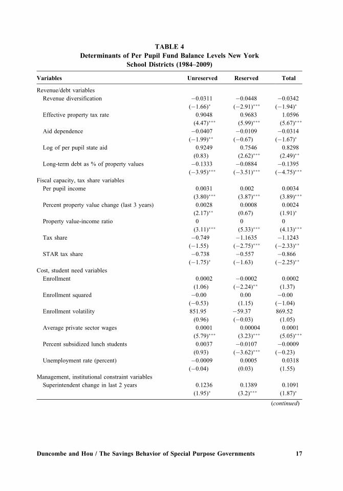
TABLE 4

Determinants of Per Pupil Fund Balance Levels New York

School Districts (1984–2009)




(�1.66)��0.0448

(�2.91)��0.0342

(�1.94)�


(4.47)��0.9683

(5.99)��1.0596

(5.67)��

Aid dependence �0.0407

(�1.99)��0.0109

(�0.67)

�0.0314

(�1.67)�


(0.83)

0.7546

(2.62)��0.8298

(2.49)��


(�3.95)��0.0884

(�3.51)��0.1395

(�4.75)��



(3.80)��0.002

(3.87)��0.0034

(3.89)��


(2.17)��0.0008

(0.67)

0.0024

(1.91)�


(3.11)��0

(5.33)��0

(4.13)��

Tax share �0.749

(�1.55)

�1.1635

(�2.75)��1.1243

(�2.33)��


(�1.75)��0.557

(�1.63)

�0.866

(�2.25)��


Enrollment 0.0002

(1.06)

�0.0002

(�2.24)��0.0002

(1.37)


(�0.53)

0.00

(1.15)

�0.00

(�1.04)

Enrollment volatility 851.95

(0.96)

�59.37

(�0.03)

869.52

(1.05)


(5.79)��0.00004

(3.23)��0.0001

(5.05)��

Percent subsidized lunch students 0.0037

(0.93)

�0.0107

(�3.62)��0.0009

(�0.23)


(�0.04)

0.0005

(0.03)

0.0318

(1.55)


Superintendent change in last 2 years 0.1236

(1.95)�0.1389

(3.2)��0.1091

(1.87)�

(continued)


purpose governments. These new results reveal the differences in savings behavior between the

two types of governments.

If fund balances represent slack, school districts with higher tax prices and with higher

property values-to-income ratios would accumulate lower savings, since voters are facing heavy

tax burdens and are therefore more apt to exert pressure on school boards to reduce the

accumulation of fund balances. As expected, the tax share and STAR tax share have the expected

negative sign and the property wealth-income ratio has a positive sign.

With regard to variables related to the cost of providing educational services, if districts act

proactively we would expect that smaller districts, those with more volatile enrollment, higher

salaries, a higher share of students in poverty, and a higher unemployment rate would

accumulate higher fund balances. The results, however, are mixed. As expected, smaller districts

are associated with higher fund balances, as are districts with more volatile enrollments. The

results for the quadratic functional form imply that at some enrollment level, fund balances will

increase with enrollment. However, given that the inflexion point is at a higher enrollment than

any district in our sample, this implies that the relationship is negative overall for New York

school districts. The coefficients for the other cost-related variables are less consistent across

models and less apt to be statistically significant.

TABLE 4 (Continued)



(�1.47)

�1.7229

(�0.89)

�3.83

(�1.56)


(0.73)

0.347

(1.93)�0.1319

(0.56)

Small city district after 1997 0.2303

(1.15)

�0.397

(�3.59)��0.0243

(0.13)

Sample size 15,367 15,367 15,367

Centered R-square 0.03 0.22 0.36


F-statistic (revenue diversification) 243.38 243.38 243.38

F-statistic (effective property tax rate) 115.12 115.12 115.12

F-statistic (aid dependence) 255.42 255.42 255.42

F-statistic (Long-term debt as% of property values) 215.16 215.16 215.16

Kleibergen-Paap rk Wald F statistic 67.73 67.73 67.73

Overidentification test (p-value) 0.28 0.05 0.12

Notes: (1) t-Statistics are in parentheses. (2) Dependent variable is the inverse hyperbolic sine transformation of per pupil

fund balance ln(Yþ (Y0.5þ 1)2). (3) All explanatory variables are lagged one year unless indicated otherwise. (4) All models

include year fixed effects and school district fixed effects. (5)Models are estimated with a linear two-step general method of

moments (GMM) estimator. (6) Endogenous variables are revenue diversification, effective tax rate, aid dependence, and

total outstanding debt as a percent of property values. Instruments for the endogenous variables are explained in the text. (7)

Hypothesis tests are based on the Newey and West (1987) method for estimating heteroskedasticity and autocorrelation-

consistent (HAC) standard errors. (8) Asterisks denote statistical significance at the 1% (��), 5% (��), and 10% (�) levels.


As for management and institutional constraints, districts that had higher superintendent

turnover in the previous two years had significantly higher fund balances. It is possible

that districts with less stable leadership are more risk averse and thereby accumulate

higher fund balances. Debt limit does not pose a statistically significant effect on savings.

Neither of the controls of small city districts are consistent in sign and significance across

models.

The overall pattern of the results from Table 3 is similar for the unreserved fund balances and

the reserved fund balances even if some of the coefficients are quite different, suggesting that

similar factors are affecting savings decisions both in the reserved and the unreserved form.

With these results, we cannot arrive at any conclusion on whether school districts as one major

type of special-purpose government are proactive or reactive in their savings behavior. This

corresponds to the patterns shown in Figure 3, where high-need rural districts have high fund

balances and high-need urban districts have relatively low fund balances.

We also tried rerunning the regressions when the dependent variable is real fund balances per

pupil. To deal with heteroscedasticity, it is common to take the natural logarithm of financial

variables. However, since fund balances can be less than or equal to zero, using a natural

logarithm will remove from the sample those school districts with negative or zero fund

balances. There are several alternative approaches for transforming variables. Table 4 reports

results using an inverse hyperbolic sine transformation.18 The signs of the coefficients in Table 4

are similar to those in Table 3, suggesting that these results are not overly sensitive to the

measure of fund balances used in the model; i.e., the results are consistent.

Figures 1 and 3 suggest that the determinants of fund balances could be quite different

between high-need rural school districts and other types of districts. To examine whether this

was the case, we estimated separate fund balance regressions for high-need rural districts and

other types of districts. The results for the unreserved and reserved fund balances are reported in

Table 5. While the directions of the relationships are the same for high-need rural and

other districts, the magnitude of the effects are in general much larger in high-need rural

districts. This is particularly the case for the fiscal variables. The coefficients on the

effective property tax rate in rural districts is three to four times higher than in other districts.

While aid dependence is not significantly related to the fund balance ratios, in high-need

districts there is a statistically significant (at the 10 percent level) and positive relationship. In

other words, high-need rural districts appear to react more strongly than other districts to

changes in fiscal variables, fiscal capacity, and tax prices. Overall, we have identified several

suggestive results, some as expected but some are understandably not. However, we have not

generated consistent evidence that the savings behavior of school districts is closely related to

the economic cycle.

18. The inverse hyperbolic sine transformation can be expressed as ln(Yþ (Y0.5þ 1)2), where Y in this case would be

per pupil unreserved fund balances. This transformation essentially uses 0 for values less than or equal to zero and

ln(Y) for values greater than zero (see Burbridge 1988; Johnson 1949). An alternative transformation is to add the

minimum value plus one to all values and then take the natural log. This approach shifts the distribution of Y but

doesn’t change the shape of the distribution. These results are available upon request.


TABLE 5

Determinants of Fund Balance Ratios Comparison of High Need Rural and Other School

Districts in New York (1984–2009)

Variables

High need rural districts Other districts

Unreserved Reserved Unreserved Reserved



(�3.23)��0.4584

(�4.67)��0.0412

(�0.71)

�0.2852

(�4.39)��


(3.22)��12.1152

(3.99)��2.5428

(4.31)��3.8634

(6.44)��

Aid dependence 0.5183

(1.73)�0.6214

(2.18)��0.0141

(�0.28)

�0.0273

(�0.46)


(0.99)

�7.8889

(�1.54)

0.9915

(1.03)

1.0179

(0.95)


(�3.99)��0.5406

(�3.96)��0.3996

(�4.07)��0.5768

(�5.13)��



(2.04)��0.0771

(2.06)��0.0088

(3.07)��0.0067

(4.37)��


(1.97)��0.0085

(�0.67)

0.0064

(1.62)

0.0064

(1.17)


(3.08)��0

(3.39)��0

(2.31)��0

(2.29)��

Tax share �13.288

(�2.77)��18.426

(�4.09)��3.576

(�2.66)��3.0263

(�2.09)��


(�0.46)

1.5066

(0.51)

1.2908

(0.64)

�8.419

(�4.08)��


Enrollment 0.0018

(0.34)

0.0001

(0.03)

0.0003

(0.95)

�0.0002

(�0.65)


(�0.02)

0.00

(0.19)

�0.00

(�0.97)

0.00

(2.22)��

Enrollment volatility 10889

(0.50)

49583

(2.63)��6423

(0.87)

9242

(1.37)


(0.88)

0.00

(0.03)

0.0001

(2.37)��0.0001

(�1.61)

Percent subsidized lunch students �0.0277

(�1.41)

�0.0375

(�1.88)��0.0034

(�0.31)

�0.0301

(�2.73)��


(�3.83)��0.1656

(1.58)

�0.039

(�0.36)

0.2912

(3.37)��


Superintendent change in last

2 years

0.7085

(1.91)��0.0601

(�0.19)

0.653

(3.91)��0.1682

(�0.99)


(�1.19)

�58.4223

(�2.82)��5.6557

(�1.2)

9.784

(0.61)

(continued)


CONCLUSIONS

The purpose of this paper was to explore the savings behavior of special-purpose governments.

School districts are the dominant type of special-purpose governments in terms of budget size

and close connection to property taxation and employment, so we have taken school districts of a

big state, NewYork, as our sample for empirical tests. Since literature on the savings behavior of

special-purpose governments does not exist, this paper is among the first study to do substantive

explorations in this important area. Our data covers three full economic cycles, thus our results

can serve as revealing, though preliminary, evidence in the research area. Given that the current

literature is exclusively on general-purpose governments, our hypotheses are built on previous

studies of state and local government savings behavior; thus, it is natural that our results have

turned out to be against our expectations in some cases. All is progress, however, toward a full

understanding of fiscal behavior of special purpose governments, which is the potential

contribution of this paper to the literature.

As one of the first explorations into the savings behavior of special-purpose governments, this

analysis has offered some preliminary findings about the savings behavior of different types of

school districts in the State of NewYork. In summary, if school districts take a proactive strategy

on their fund balance levels, wemight expect that districts that are potentially the most vulnerable

to fiscal shocks will accumulate the highest relative fund balances. For example, districts with

TABLE 5 (Continued)

Variables

High need rural districts Other districts

Unreserved Reserved Unreserved Reserved


(1.72)�0.1251

(0.13)

0.4341

(1.05)

0.7621

(1.81)�

Small city district after 1997 �0.4271

(�0.44)

�1.168

(�1.17)

1.1943

(3.86)��2.7961

(�7.45)��

Sample size 3,765 3,765 11,602 11,602

Centered R-square 0.00 0.34 0.05 0.37


F-statistic (revenue diversification) 33.99 33.99 220.96 220.96

F-statistic (effective property tax rate) 28.31 28.31 408.81 408.81

F-statistic (aid dependence) 13.86 13.86 200.05 200.05

F-statistic (long-term debt as% of property values) 55.37 55.37 298.35 298.35

Kleibergen-Paap rk Wald F statistic 13.192 13.192 45.07 45.07

Overidentification test (p-value) 0.6614 0.9727 0.07 0.17

Notes: (1) t-Statistics are in parentheses. (2) Dependent variable is the specified general fund balance as percent of operating

spending. (3) All explanatory variables are lagged one year unless indicated otherwise. (4) All models include year fixed

effects and school district fixed effects. (5) Models are estimated with a linear two-step general method of moments (GMM)

estimator. (6) Endogenous variables are revenue diversification, effective tax rate, aid dependence, and total outstanding

debt as a percent of property values. Instruments for the endogenous variables are explained in the text. (7) Hypothesis tests

are based on the Newey and West (1987) method for estimating heteroskedasticity and autocorrelation-consistent (HAC)

standard errors. (8) Asterisks denote statistical significance at the 1% (��), 5% (��), and 10% (�) levels.


high tax rates, are more aid dependent or smaller, have lower fiscal capacity or higher costs, and

should maintain higher unreserved fund balances. Our findings suggest that savings strategies

vary across types of districts. Small, rural, high-need districts do have higher fund balances than

larger, wealthier districts, on average. However, high-need urban districts with low property

wealth and income and higher student poverty tend tomaintain lower fund balances. Districts that

are more dependent on state aid and with higher debt burdens tend to have lower balances, but

districts with high property tax rates have higher fund balances. It does appear that districts in

which residents shoulder a higher share of property taxes do keep lower fund balances, suggesting

that residents may exert pressure on school boards to keep tax rates lower. We find that these

relationships are even stronger for high-need rural districts, which is consistent with the

hypothesis that they are more proactive in using savings to buffer against fiscal shocks.

A second major finding is that the fund balance determinants for reserved funds are similar to

those for unreserved funds. We have not seen major differences in the direction of the

relationships or their statistical significance. These findings indicate that school districts consider

both types of funds when making savings decisions. The fact that reserved fund balances of New

York school districts were on average four times higher than unreserved balances in FY2009

suggests that these districts had been strategically using reserve funds as a general savings device.

The usual caveats apply. School districts vary in a state under the same operating

environment; they may vary even more across states. We have examined only school districts in

the State of NewYork; more research is needed to determine whether our findings for NewYork

are applicable in other states and to understand how state regulations on the use of reserve funds

affect their use by local governments. Further, we have examined only school districts, which are

merely one among different kinds of special-purpose governments. We look forward to studies

that dissect the savings behavior of other types so as to generate more generic findings on their

behavioral patterns for a better and fuller understanding of this important fiscal behavior at the

local level. Finally, this paper has been mostly an empirical exploration; we are yet to develop a

fully-fledged theory on the savings behavior of local governments, which is not done in this

paper but will be the work in our subsequent papers.

REFERENCES

Boyd, Don and Victoria Wachino. 2004. “Is the State Fiscal Crisis Over? A 2004 State Budget Update.” Issue

Paper of the Kaiser Commission on Medicaid and the Uninsured. (January): 1–9.

Burbridge, John. 1988. “Alternative Transformations to Handle Extreme Values of the Dependent Variable.”

Journal of the American Statistical Association. 83 (401): 123–127.

Davis, Michelle. 2008. “Financial Crisis Now Striking Home to School Districts.” Education Week. 28 (9): 8.

Duncombe, William and John Yinger. 1997. “Why Is It So Hard to Help Central-City Schools?” Journal of

Public Policy Analysis and Management. 16 (1): 85–113.

———. 2000. “Financing Higher Student Performance Standards: The Case of New York State,” Economics

of Education Review. 19 (October): 363–386.

———. 2008. “Measurement of Cost Differentials.” In Handbook of Research in Education Finance and

Policy. edited by, Helen Ladd and Edward Fiske, 238–256. New York, NY: Routledge.

Duncombe,William, JerryMiner, and John Ruggiero. 1997. “Empirical Evaluation of BureaucraticModels of

Inefficiency.” Public Choice. 93 (October): 1–18.


Eom, Tae Ho, William Duncombe, and John Yinger. 2011. “The Unintended Consequences of Property Tax

Relief: New York’s STAR Program.” 2011 AEFP Annual Conference, Washington, DC.

Gianakis, Gerasimos andDouglas Snow. 2007. “The Implementation andUtilization of Stabilization Funds by

Local Governments in Massachusetts.” Public Budgeting & Finance. 27 (Spring): 86–103.

Hendrick, Rebecca. 2006. “The Role of Slack in Local Government Finance.” Public Budgeting & Finance.

26 (Spring): 14–46.

Hou, Yilin. 2003. “What Stabilizes State General Fund Expenditures in Downturn Year—Budget

Stabilization Fund or General Fund Unreserved Undesignated Balance?” Public Budgeting & Finance.

23 (Fall): 64–91.

———. 2004. “Budget Stabilization Fund: Structural Features of the Enabling Legislation and Balance

Levels.” Public Budgeting & Finance. 24 (Fall): 38–64.

———. 2005. “Fiscal Reserves and State Own-source Expenditure in Downturns.” Public Finance Review 33

(January): 117–144.

Hou, Yilin and William Duncombe. 2008. “State Saving Behavior: Effects of Two Fiscal and Budgetary

Institutions.” Public Budgeting & Finance. 28 (Winter): 48–67.

Johnson, N.L. 1949. “Systems of Frequency Curves Generated by Methods of Translation.” Biometrica. 36

(June): 149–176.

Kroszner, Randall S. and Thomas S. Stratmann. 2000. “Congressional Committees as Reputation-building

Mechanisms.” Business and Politics. 2 (1): 35–52.

Ladd, Helen and John Yinger. 1994. “The Case for Equalizing Aid.” National Tax Journal. 47 (1): 221–224.

Marlowe, Justin. 2005. “Fiscal Slack and Counter-Cyclical Expenditure Stabilization: A First Look at the

Local Level.” Public Budgeting & Finance. 25 (Fall): 48–72.

McNichol, Elizabeth and Iris Lav. 2009. “New Fiscal Year Brings No Relief from Unprecedented State

Budget Problems.” Working Paper, Center on Budget and Policy Priorities, July 29.

National Conference of State Legislatures (NCSL). 2009. State Budget Update: July 2009. Washington, DC:

National Conference of State Legislatures (NCSL).

Newey, Whitney K. and Kenneth D. West. 1987. “A Simple, Positive Semi-definite, Heteroskedasticity and

Autocorrelation Consistent Covariance Matrix.” Econometrica. 55 (3): 703–708.

New York State Education Department (NYSED). 2010. “Definitions of Need/Resource-Capacity Categories

of New York State School Districts.” New York State Board of Regents Proposal on State Aid to School

Districts for School Year 2010–11. Albany, NY: SED.

———. 2011. “School District Financial Condition.” Memo from Valerie Grey and John King, Jr. to the

Regents Committee on Audits, Budget and Finance and Regents Subcommittee on State Aid. June, 7.

Smith, Edward. 2009. “A Grim Forecast.” State Legislatures. (February): 12–15.

Staiger, Douglas and James H. Stock. 1997. “Instrumental Variables Regression with Weak Instruments.”

Econometrica. 65 (3): 557–586.

Stock, James H. and Motohiro Yogo. 2005. “Testing for Weak Instruments in Linear IV Regression.” In

Identification and Inference for Econometric Models: Essays in Honor of Thomas Rothenberg, edited by,

James H. Stock and D.W.K. Andrews, 80–108. New York, NY: Cambridge University Press.

U.S. Census Bureau. 2011a. Public Education Finances: 2009. G09-ASPEF. Washington, DC: U.S.

Government Printing Office.

———. 2011b. “State and Local Government Finances Summary; 2009.”Governments Division Briefs, GO9-

ALFIN (October).

Wang, Wen and Yilin Hou. 2012. “Do Local Governments Save and Spend Across Budget Cycles? Evidence

from North Carolina.” American Review of Public Administration. 42 (2): 152–169.

Wintrobe, Ron. 1997. “Modern Bureaucratic Theory.” In Perspectives on Public Choice: A Handbook. edited

by, Dennis C. Mueller, 429–454. New York, NY. Cambridge University Press.

Wooldridge, Jeffrey M. 2003. Introductory Econometrics: A Modern Approach. Second Edition. Mason, OH:

South-Western.


Documents

The Savings Behavior of Special Purpose Governments: A Panel Study of New York School Districts