Embed Size (px)
Citation preview
The Role of Financial Market Development on Financial
Contagion: Evidence from Selected Asian Economies (This version: 14 October 2016)
By: Iman Badrudin1
Abstract
This paper seeks to examine the role of financial sector development in cushioning the
extent of financial contagion in Asian economies since the 2008 Global Financial Crisis.
This study looks at Thailand, Indonesia, Malaysia and Korea, countries that were
severely affected during the 1997 Asian Financial Crisis. This paper also attempts to
distinguish the ability of current Asian financial systems in dealing with global and
regional shocks. The empirical results broadly suggest that financial market
development has played significant roles in the management of financial contagion for
these Asian economies. The effects on equity contagion are comparatively stronger
than for currency contagion. In particular, the size of the banking system and the
degree of financial openness matters to reduce stock market contagion, while higher
levels of adequate reserves does have some offsetting effects during currency shocks.
Present market conditions also appear to show signs of greater resilience against a
regional equity shock similar to what was experienced in 1997.
Any views expressed are solely those of the author and so cannot be taken to represent those of
Bank Negara Malaysia. This paper should therefore not be reported as representing the views of
Bank Negara Malaysia.
1 Author can be reached at [email protected]
2
Contents
1. Introduction 1
1.1 Background and motivation 1
1.2 Research Objective 5
2. Empirical strategy and data 8
2.1 Stage 1: SVAR analysis to identify common global and regional shocks 8
2.2 Stage 2: Determining presence of financial contagion 11
2.4 Stage 3: Estimating impact of financial market development 13
2.4 Data 16
3. Empirical results 17
3.1 Stage 1: SVAR impulse response analysis 17
3.2 Stage 2: Identifying presence of financial contagion 20
3.3 Stage 3: Assessing the impact of financial market development on contagion 22
3.3.1 Role of market development during stock market contagion 23
3.3.2 Role of market development during currency contagion 25
3.3.3 Simulating a stronger regional shock 27
4. Conclusion and policy recommendations 29
References 32
Appendix A: Empirical strategy 35
A1 Alternative formulation of the Forbes and Rigobon test of contagion 35
Appendix B: Empirical results 36
B1 Summary statistics 36
B2 Impulse response graphs 37
B3 Stage 3 estimation results 40
1
1. Introduction
1.1 Background and motivation
Financial market development has always been an important agenda for Asian
economies. This is due to the recognition that market development can facilitate long-
run economic growth, enable easier government borrowing and enhance general
welfare; all while simultaneously acting as a conduit for domestic monetary policy
(Obstfeld, 2009). Nevertheless, the Asian Financial Crisis (AFC) in 1997 had highlighted
inherent weaknesses in both the economy and financial systems of the countries at the
epicentre of the crisis, i.e. Thailand, Indonesia, Malaysia and Korea. In the period
leading to the crisis, domestic investments were mostly funded through foreign
borrowings, while prudential regulation and supervision failed to keep up with financial
liberalisation (Lindgren et al, 1999). Following the crisis, these economies underwent
various macroeconomic, corporate and financial sector reforms aimed at strengthening
fundamentals, improving resilience towards unfavourable shocks and promoting
regional financial integration (Park, 2011).
Post Asian crisis financial sector reforms had focused on restructuring the banking
system’s balance sheets, mostly through deleveraging processes and recapitalization.
These efforts worked to reduce external vulnerability, as evidenced by the resilience of
Asian economies during the 2008 Global Financial Crisis (GFC)2. These reforms were
also accompanied by carefully sequenced financial market development that was
supported by better regulation. In this respect, market development was intended to
2 While Asian economies were not spared from the economic and financial shocks of the 2008 GFC, by 2010 most countries had experienced economic recovery that prompted the withdrawal of monetary stimulus that was implemented during the crisis.
2
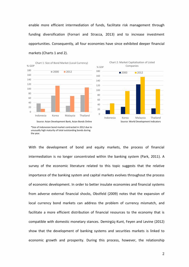
enable more efficient intermediation of funds, facilitate risk management through
funding diversification (Fornari and Stracca, 2013) and to increase investment
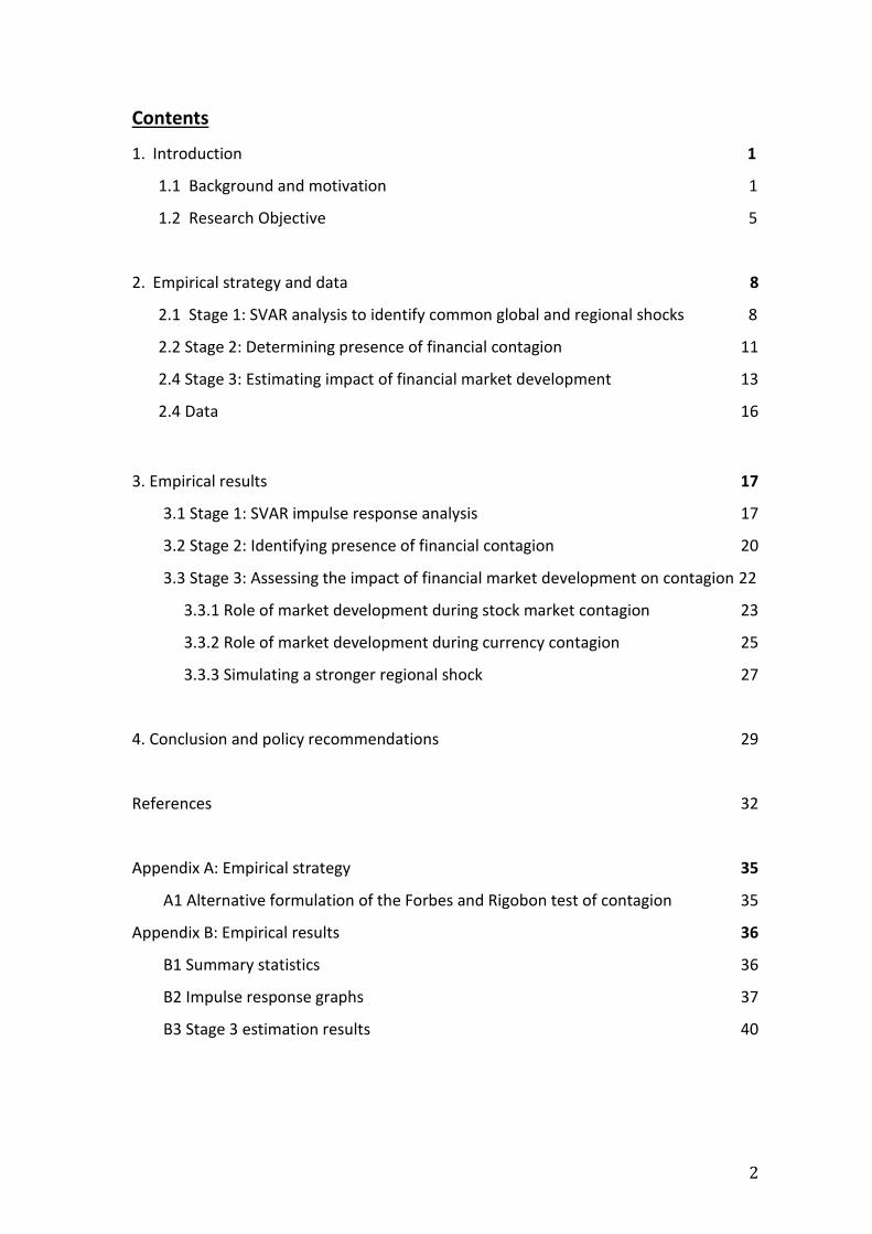
opportunities. Consequently, all four economies have since exhibited deeper financial
markets (Charts 1 and 2).
With the development of bond and equity markets, the process of financial
intermediation is no longer concentrated within the banking system (Park, 2011). A
survey of the economic literature related to this topic suggests that the relative
importance of the banking system and capital markets evolves throughout the process
of economic development. In order to better insulate economies and financial systems
from adverse external financial shocks, Obstfeld (2009) notes that the expansion of
local currency bond markets can address the problem of currency mismatch, and
facilitate a more efficient distribution of financial resources to the economy that is
compatible with domestic monetary stances. Demirgüç-Kunt, Feyen and Levine (2012)
show that the development of banking systems and securities markets is linked to
economic growth and prosperity. During this process, however, the relationship
0
20
40
60
80
100
120
140
160
180
Indonesia Korea Malaysia Thailand
% GDP Chart 1: Size of Bond Market (Local Currency)
2000 2012
0
20
40
60
80
100
120
140
160
180
Indonesia Korea Malaysia Thailand
% GDP
Chart 2: Market Capitalisation of Listed Companies
2000 2012
Source: Asian Development Bank, Asian Bonds Online Source: World Development Indicators
*Size of Indonesian bond market contracted in 2012 due to unusually high maturity of total outstanding bonds during the year.
3
between traditional banking and economic activity tends to weaken amid
strengthening links between capital markets and economic growth. Boot and Thakor
(1997) and Weinstein and Yafeh (1998) also suggest that while the financial services
offered by banks and capital markets are different but complementary, financing via
the capital market tends to become more relevant as the economy grows and the
number of projects or investments that require customized financing needs increases.
As such, capital markets that are not constrained by standardized contracts and easily
collateralised capital inputs would best meet these requirements. Thus it is not
surprising that greater development of capital markets is likely to play a relatively
stronger role in supporting economic activity (Demirgüç-Kunt, Feyen and Levine, 2012).
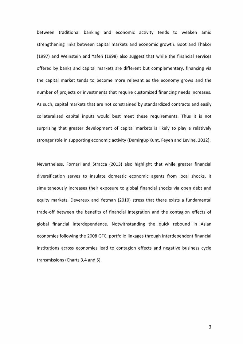
Nevertheless, Fornari and Stracca (2013) also highlight that while greater financial
diversification serves to insulate domestic economic agents from local shocks, it
simultaneously increases their exposure to global financial shocks via open debt and
equity markets. Devereux and Yetman (2010) stress that there exists a fundamental
trade-off between the benefits of financial integration and the contagion effects of
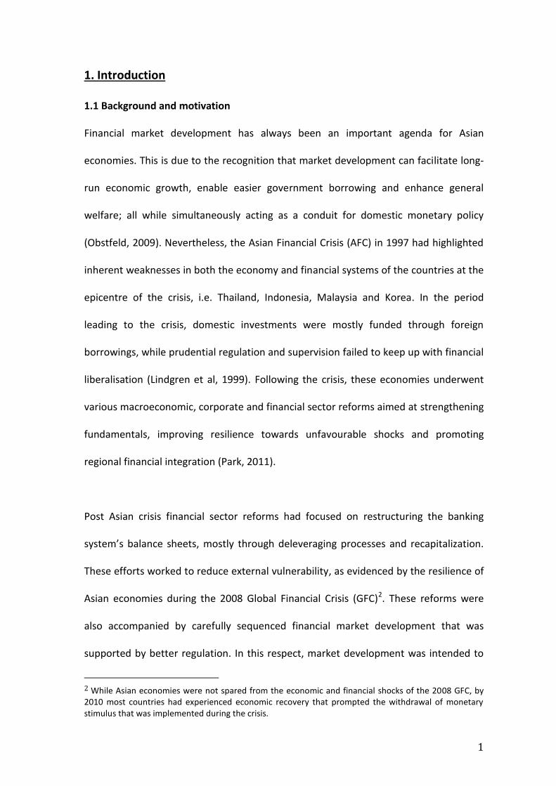
global financial interdependence. Notwithstanding the quick rebound in Asian
economies following the 2008 GFC, portfolio linkages through interdependent financial
institutions across economies lead to contagion effects and negative business cycle
transmissions (Charts 3,4 and 5).
4
-40 -30 -20 -10 0 10 20
MYR
KRW
THB
IDR
Chart 3: Exchange Rate Movement (% change)
2010 2009 2008
-100.0
-60.0
-20.0
20.0
60.0
100.0
140.0
180.0
20
05
20
06
20
07
20
08
20
09
20
10
20
11
20
12
20
13
20
14
% Chart 4: Annual % Change in Equity Indices
Indonesia Korea Malaysia
Thailand US
-4
-2
0
2
4
6
8
10
20
05
20
06
20
07
20
08
20
09
20
10
20
11
20
12
20
13
20
14
% Chart 5: Real GDP
G7 Indonesia Korea
Malaysia Thailand
Source: Bloomberg
*IDR: Indonesian Rupiah; THB: Thai Baht; KRW: Korean Won; MYR: Malaysian Ringgit
Source: Bloomberg
Source: IMF World Economic Outlook
5
The impact of the 2008 GFC was different from the AFC in 1997 not only because the
sharp reversal in capital flows was due to the crisis in advanced economies, but also
because the Asian economies studied in this paper could not rely on exports to drive
their recovery despite the depreciation of their currencies (Ozkan and Unsal, 2012).
Given the quick turnaround of Asian economies in a weak external environment, this
strongly suggests that the existing domestic economic and financial structures, which
are a product of the post-AFC reforms, have had a positive impact on their ability to
withstand adverse shocks. Since the 2008 GFC, these financial systems have also been
subjected to further external shocks due to heightened uncertainty and volatility in
global financial markets. These include the implementation and withdrawal of the
United States (US) Federal Reserve’s Quantitative Easing (QE) programmes, as well as
investors’ concerns over the relative strength of macroeconomic fundamentals within
the region.
1.2 Research objective
Given that the financial markets of the economies that were severely affected during
the 1997 AFC are now much more developed, it is likely that these factors have had
some influence during the recent episodes of financial contagion. Therefore, this paper
will seek to answer 2 key questions:
i. Has financial sector development helped Asian economies cushion the extent of
financial contagion since the 2008 Global Financial Crisis? If so, which aspect of
financial sector development matters most for this purpose?
ii. Are there differences in the ability of current Asian financial systems to
withstand global and regional shocks?
6
This research differs from other studies of financial contagion, as it will examine the
role of financial market development in totality rather than focus on one aspect, i.e.
financial integration, as most studies have done. Chami, Fullenkamp and Sharma (2009)
suggest a framework for financial market development that relies upon the existence
and actions of participants (liquidity providers, regulators, international and domestic
borrowers and lenders) whose presence is essential for the efficient functioning of
markets. Following the recommendations in the International Monetary Fund’s (IMF)
2005 ‘Financial Sector Assessment: A Handbook’, financial structure and development
should capture the size, breadth and composition of the financial system. Therefore,
the impact of other aspects of market development in managing financial contagion,
particularly those recommended by the IMF, will also be considered. These may include
the adequacy of foreign reserves, size of the domestic banking system, equity and bond
markets, as well as the degree of financial openness.
The analysis in this paper is divided into three main stages. In the first stage, global and
regional financial shocks are tested via a structural vector autoregression (SVAR) to
ensure that they have had significant impact across all four economies studied in this
paper. Next, a two sample or heteroskedastic t-test is carried out to determine
whether financial contagion occurred in stock and currency markets during these
identified shocks. Finally, we estimate the effects of various aspects of market
development for each economy during separate periods of financial contagion using
Ordinary Least Squares (OLS) regressions. In this section, we also attempt to simulate
stronger regional shocks by replicating the magnitude of stock and currency contagion
7
during the AFC, and testing the performance of present levels of market development
against these financial shocks.
The key findings of this paper suggests that while on average, financial market
development has had significant effects in the management of financial contagion for
these Asian economies, the impact appears to be more constraining for contagion in
the stock market. In particular, the size of the banking system and the degree of
financial openness matters to minimize stock market contagion, while higher levels of
adequate international reserves does have some offsetting effects during currency
shocks. Nevertheless, present market conditions appear to show signs of greater
resilience against a major regional shock similar to that during the AFC.
The rest of the paper is organized as follows. Section 2 provides detailed information
on the empirical strategy and data used in this study to examine the impact of market
development on several types of financial contagions. Section 3 then provides a
comprehensive discussion of the results, while Section 4 concludes and offers some
policy recommendations and potential areas for further research on the topic.
8
2. Empirical strategy and data
The empirical strategy of this study will be broadly based on the methodology used by
Baig and Goldfajn (1999), albeit with some modifications to ensure that the key
research questions outlined in Section 1 are addressed. As such, the sequence of
methods is divided into three main stages.
2.1 Stage 1: SVAR analysis to identify common global and regional shocks
A SVAR model is used to identify global and regional shocks that have had comparable
effects across the Asian financial markets being studied. A SVAR approach is chosen
over the vector autoregression (VAR) method used in Baign and Goldfajn (1999) to
differentiate the movements in indicators that reflect financial contagion caused by a
shock in either global or regional financial markets by imposing restrictions on the long-
run characteristics of the variables (Dungey et al, 2003). These restrictions enable the
impulse response functions to be interpreted as the impact of an increase in the shock
variable to the structural innovation of the dependent variables.
The following global and regional financial shocks will be tested:
i. The 2008 collapse of Lehman Brothers3, which effectively triggered the Global
Financial Crisis. The Chicago Board Options Exchange’s (CBOE) Market Volatility
Index (VIX) will be used to proxy this shock. The VIX index is largely an
asymmetric measure of investor confidence; much stronger when stock
markets plunge due to adverse financial shocks compared to when measuring
3 The collapse of Lehman Brothers on 15 September 2008 is widely viewed as the key trigger event for
the Global Financial Crisis as it lead to a severe loss of confidence in the global financial system (International Organization of Supreme Audit Institutions, 2010).
9
investor confidence during a market rally (Whaley, 2008). As such, the
asymmetric nature of the VIX index would provide a more robust reflection of
global market turbulence during the Lehman collapse.
ii. The implementation and scaleback of quantitative easing (QE) in the United
States. These events were unlike anything that had occurred in global financial
markets previously in terms of magnitude and impact to global monetary
conditions. To proxy for these shocks, the US 5 year sovereign yields are used to
reflect the impact of the programme announcements and implementation. In
particular, only the implementation of the first QE programme (QE1) will be
tested, whereas for the programme withdrawal, the shocks will cover the
period of market tantrum due to misinterpretation of hints by the then Federal
Reserve Chairman, Ben Bernanke, over the timing of a scaleback in the QE
programme, as well as the actual tapering of the Federal Reserve’s asset
purchases.
iii. In terms of regional financial shocks, the case of twin deficit concerns
originating from Indonesia in 2013 will be tested as it was considered a trigger
for investor fears over weakening fiscal and current account fundamentals
within the region. To represent this shock, the 5 year Indonesian sovereign yield
will be used to reflect the corresponding outlook downgrade by Standard and
Poor (S&P) due to concerns over its twin deficits.
The impact of the shocks listed above will be analysed on three main market indicators
that are likely to reflect any immediate financial contagion driven by shifts in investors’
portfolio funds. These indicators include daily changes in domestic stock market
10
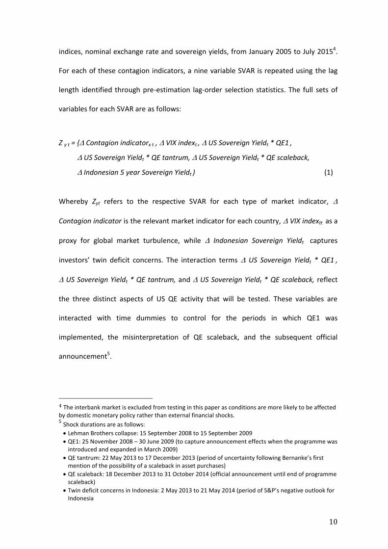
indices, nominal exchange rate and sovereign yields, from January 2005 to July 20154.
For each of these contagion indicators, a nine variable SVAR is repeated using the lag
length identified through pre-estimation lag-order selection statistics. The full sets of
variables for each SVAR are as follows:
Z y t = { Contagion indicatorx t , VIX indext , US Sovereign Yieldt * QE1 ,
US Sovereign Yieldt * QE tantrum, US Sovereign Yieldt * QE scaleback,
Indonesian 5 year Sovereign Yieldt ) (1)
Whereby Zyt refers to the respective SVAR for each type of market indicator,
Contagion indicator is the relevant market indicator for each country, VIX indextt as a
proxy for global market turbulence, while Indonesian Sovereign Yieldt captures
investors’ twin deficit concerns. The interaction terms US Sovereign Yieldt * QE1 ,
US Sovereign Yieldt * QE tantrum, and US Sovereign Yieldt * QE scaleback, reflect
the three distinct aspects of US QE activity that will be tested. These variables are
interacted with time dummies to control for the periods in which QE1 was
implemented, the misinterpretation of QE scaleback, and the subsequent official
announcement5.
4 The interbank market is excluded from testing in this paper as conditions are more likely to be affected by domestic monetary policy rather than external financial shocks. 5 Shock durations are as follows:
Lehman Brothers collapse: 15 September 2008 to 15 September 2009
QE1: 25 November 2008 – 30 June 2009 (to capture announcement effects when the programme was introduced and expanded in March 2009)
QE tantrum: 22 May 2013 to 17 December 2013 (period of uncertainty following Bernanke’s first mention of the possibility of a scaleback in asset purchases)
QE scaleback: 18 December 2013 to 31 October 2014 (official announcement until end of programme scaleback)
Twin deficit concerns in Indonesia: 2 May 2013 to 21 May 2014 (period of S&P’s negative outlook for Indonesia
11
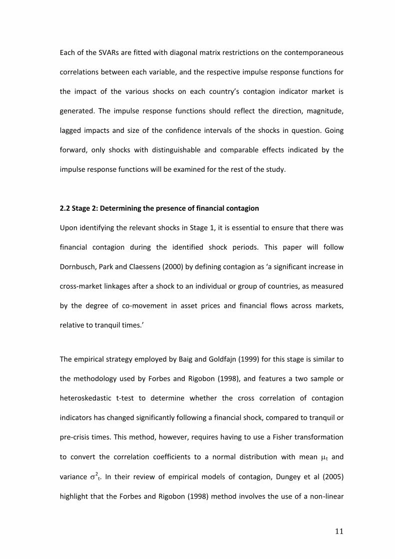
Each of the SVARs are fitted with diagonal matrix restrictions on the contemporaneous
correlations between each variable, and the respective impulse response functions for
the impact of the various shocks on each country’s contagion indicator market is
generated. The impulse response functions should reflect the direction, magnitude,
lagged impacts and size of the confidence intervals of the shocks in question. Going
forward, only shocks with distinguishable and comparable effects indicated by the
impulse response functions will be examined for the rest of the study.
2.2 Stage 2: Determining the presence of financial contagion
Upon identifying the relevant shocks in Stage 1, it is essential to ensure that there was
financial contagion during the identified shock periods. This paper will follow
Dornbusch, Park and Claessens (2000) by defining contagion as ‘a significant increase in
cross-market linkages after a shock to an individual or group of countries, as measured
by the degree of co-movement in asset prices and financial flows across markets,
relative to tranquil times.’
The empirical strategy employed by Baig and Goldfajn (1999) for this stage is similar to
the methodology used by Forbes and Rigobon (1998), and features a two sample or
heteroskedastic t-test to determine whether the cross correlation of contagion
indicators has changed significantly following a financial shock, compared to tranquil or
pre-crisis times. This method, however, requires having to use a Fisher transformation
to convert the correlation coefficients to a normal distribution with mean t and
variance 2t. In their review of empirical models of contagion, Dungey et al (2005)
highlight that the Forbes and Rigobon (1998) method involves the use of a non-linear
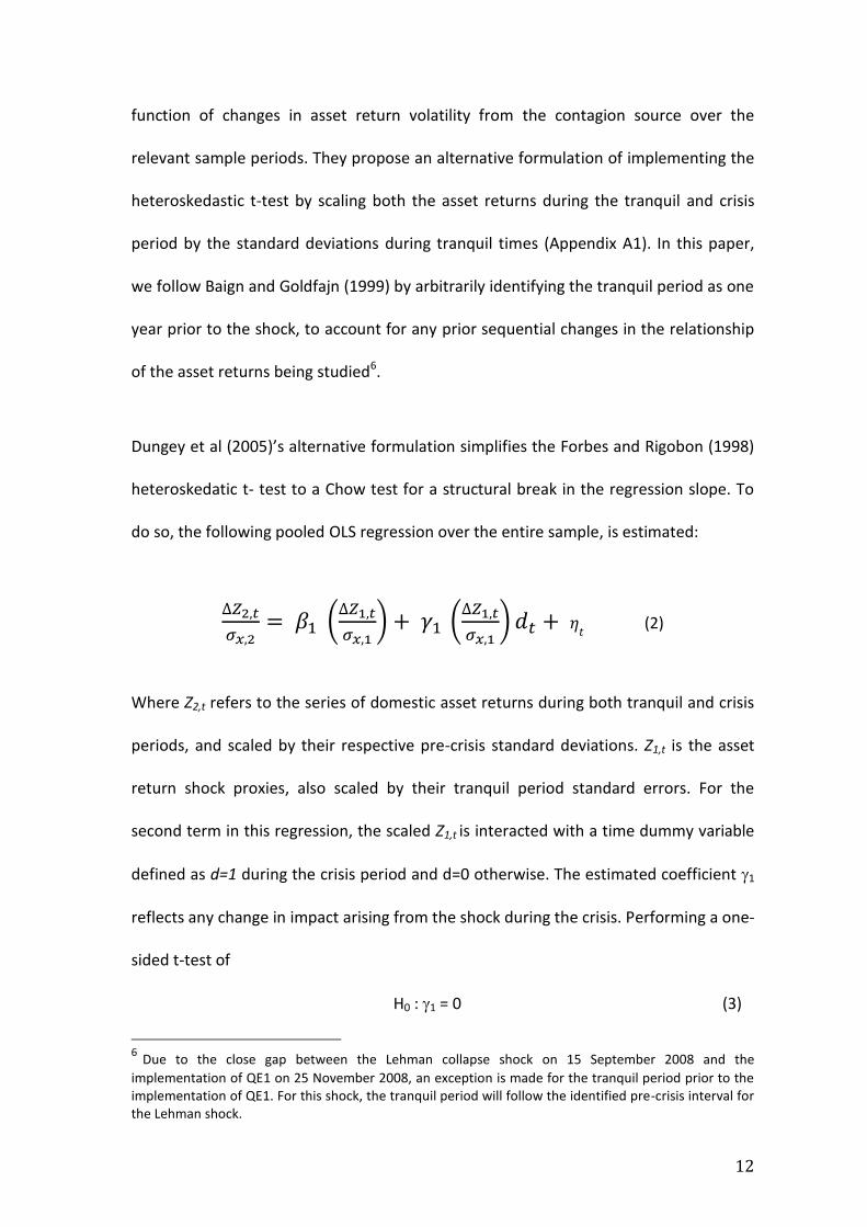
12
function of changes in asset return volatility from the contagion source over the
relevant sample periods. They propose an alternative formulation of implementing the
heteroskedastic t-test by scaling both the asset returns during the tranquil and crisis
period by the standard deviations during tranquil times (Appendix A1). In this paper,
we follow Baign and Goldfajn (1999) by arbitrarily identifying the tranquil period as one
year prior to the shock, to account for any prior sequential changes in the relationship
of the asset returns being studied6.
Dungey et al (2005)’s alternative formulation simplifies the Forbes and Rigobon (1998)
heteroskedatic t- test to a Chow test for a structural break in the regression slope. To
do so, the following pooled OLS regression over the entire sample, is estimated:
∆𝑍2,𝑡
𝜎𝑥,2= 𝛽1 (
∆𝑍1,𝑡
𝜎𝑥,1) + 𝛾1 (
∆𝑍1,𝑡
𝜎𝑥,1) 𝑑𝑡 + 𝜂
𝑡 (2)
Where Z2,t refers to the series of domestic asset returns during both tranquil and crisis
periods, and scaled by their respective pre-crisis standard deviations. Z1,t is the asset
return shock proxies, also scaled by their tranquil period standard errors. For the
second term in this regression, the scaled Z1,t is interacted with a time dummy variable
defined as d=1 during the crisis period and d=0 otherwise. The estimated coefficient 1
reflects any change in impact arising from the shock during the crisis. Performing a one-
sided t-test of
H0 : 1 = 0 (3)
6 Due to the close gap between the Lehman collapse shock on 15 September 2008 and the
implementation of QE1 on 25 November 2008, an exception is made for the tranquil period prior to the implementation of QE1. For this shock, the tranquil period will follow the identified pre-crisis interval for the Lehman shock.
13
will indicate whether or not the time dummy contributes any additional information on
the relationship between the shock variable and the domestic indicator of financial
contagion. A significant change in the relationship of the variables will suggest the
presence financial contagion during the period.
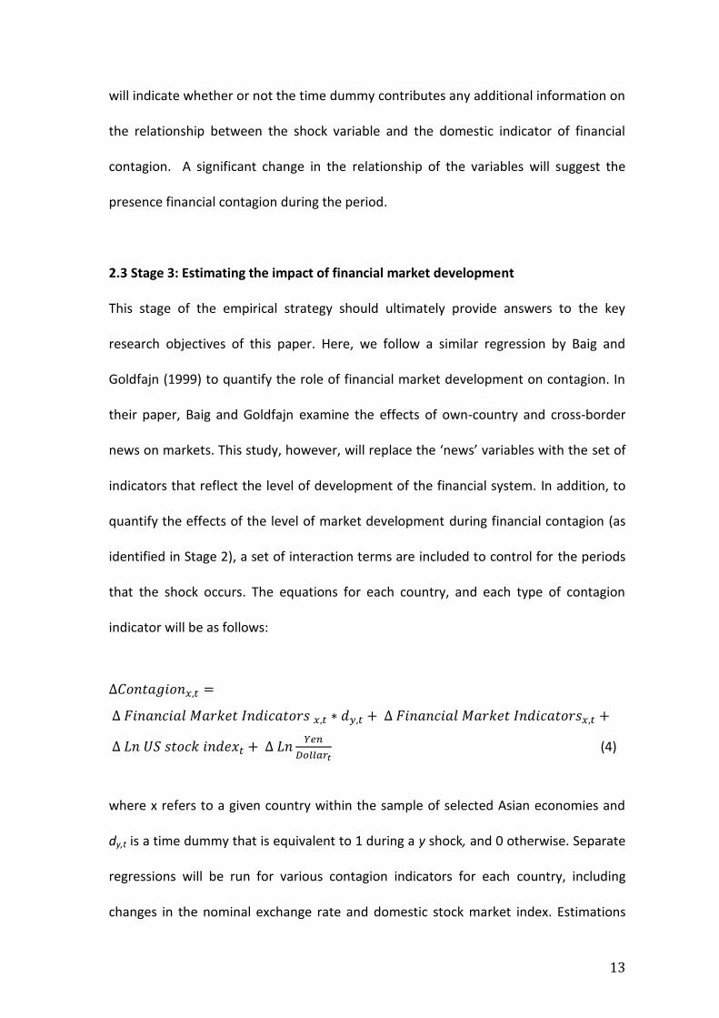
2.3 Stage 3: Estimating the impact of financial market development
This stage of the empirical strategy should ultimately provide answers to the key
research objectives of this paper. Here, we follow a similar regression by Baig and
Goldfajn (1999) to quantify the role of financial market development on contagion. In
their paper, Baig and Goldfajn examine the effects of own-country and cross-border
news on markets. This study, however, will replace the ‘news’ variables with the set of
indicators that reflect the level of development of the financial system. In addition, to
quantify the effects of the level of market development during financial contagion (as
identified in Stage 2), a set of interaction terms are included to control for the periods
that the shock occurs. The equations for each country, and each type of contagion
indicator will be as follows:
∆𝐶𝑜𝑛𝑡𝑎𝑔𝑖𝑜𝑛𝑥,𝑡 =
∆ 𝐹𝑖𝑛𝑎𝑛𝑐𝑖𝑎𝑙 𝑀𝑎𝑟𝑘𝑒𝑡 𝐼𝑛𝑑𝑖𝑐𝑎𝑡𝑜𝑟𝑠 𝑥,𝑡 ∗ 𝑑𝑦,𝑡 + ∆ 𝐹𝑖𝑛𝑎𝑛𝑐𝑖𝑎𝑙 𝑀𝑎𝑟𝑘𝑒𝑡 𝐼𝑛𝑑𝑖𝑐𝑎𝑡𝑜𝑟𝑠𝑥,𝑡 +
∆ 𝐿𝑛 𝑈𝑆 𝑠𝑡𝑜𝑐𝑘 𝑖𝑛𝑑𝑒𝑥𝑡 + ∆ 𝐿𝑛𝑌𝑒𝑛
𝐷𝑜𝑙𝑙𝑎𝑟𝑡 (4)
where x refers to a given country within the sample of selected Asian economies and
dy,t is a time dummy that is equivalent to 1 during a y shock, and 0 otherwise. Separate
regressions will be run for various contagion indicators for each country, including
changes in the nominal exchange rate and domestic stock market index. Estimations
14
will also account for on-going global financial conditions7, which is proxied for by the
US S&P500 stock index and the Yen-Dollar 8 exchange rate. Financial market
development indicators will be based on the IMF sectoral indicators of financial
development that are publicly available. Specifically, this study will take into account
the following aspects of market development:
i. Adequacy of foreign exchange reserves to mitigate excessive volatility in the
domestic currency. This is measured by international reserves as a percentage
of money supply (M2).
ii. Bank deposits as a percentage of GDP, which serves as an indicator of the
banking system’s available sources of funds. A higher ratio suggests greater size
and depth of the banking system. While a banking system that is largely reliant
on stable long-term deposits as its main source of funds could mean that there
is a lack of financial innovation, lessons from the GFC have highlighted the need
for financial institutions to fund their business activity via prudent channels to
avoid contagion effects in the event of a liquidity squeeze in financial markets
(OECD, 2012).
7 These regressions do not control for country specific macroeconomic variables (e.g. nominal GDP,
inflation, current account balance and the Government’s fiscal balance) due to concerns surrounding potential multicollinearity between these variables and financial market development indicators. As mentioned in Section 1, there may be causality among these factors. 8 The Yen-Dollar exchange rate is used as a measure of global risk aversion. Botman, de Carvalho Filho
and Lam (2013) provide support for the yen’s safe heaven currency status during periods of global risk aversion. The yen’s appreciation in response to global risk aversion is mainly driven by portfolio rebalancing through offshore derivative transactions.
15
iii. External debt9 as a percentage of GDP to measure the degree of financial
openness, given that it reflects the level of foreign participation in the domestic
financial system.
iv. Liquidity of domestic stock markets, where depending on the type of data
available for each country, is proxied for by either monthly traded volume,
turnover, or new issuances in share units10. A liquid stock market should in
theory be less susceptible to contagion effects due to the greater presence of
participants to offset any sell-off pressure.
v. Total outstanding bonds as a percentage of GDP as a measure of bond market
size. A higher ratio would reflect a more liquid market that should be capable of
absorbing contagion shocks.
As per IMF recommendation, the variables for each country (except for stock market
liquidity) have been scaled by their respective nominal GDP or broad money11. This is
done to enable valid cross-country comparisons. While fluctuations in these ratios may
be due to changes in the denominator, given that these economies have exhibited
similar business cycle patterns during the period of study, these ratios can be
considered reliable measures of market development.
9 Gross external debt is defined as the outstanding amount of those actual current (and not contingent)
liabilities that require payments of interest and /or principal by the debtor at some point in the future. These debts are owed by residents of an economy to non-residents. 10
Stock market liquidity for Malaysian equity is reflected by monthly stock turnover in million units. For Korea and Indonesia, the same indicator is represented by the monthly volume of shares traded, while the number of new stock issuances in Thailand for each month is used as a proxy for market liquidity. 11
All scaled variables are expressed as a percentages, not ratios. E.g. 70% is entered as 70 and not 0.7.
16
The hypothesis is that greater financial market development should help to cushion the
impact of shocks on contagion. As such, the coefficients on these variables are
expected to have constraining effects on contagion.
2.4 Data
Data coverage in this empirical study ranges from January 2005 to July 2015. Stages 1
and 2 rely on daily financial data extracted from Bloomberg. For Stage 3, these data
were converted to monthly frequency by taking their end-month values. Country
specific macroeconomic fundamentals were obtained from Bloomberg, IMF
International Financial Statistics and World Economic Outlook databases, while
indicators of financial market development were sourced from Bloomberg and national
central bank databases.
Where necessary in all stages, the log-linear functional form is used to reduce the
skewness of distribution and seasonality effects were removed for the relevant data. In
most cases, the estimations are run on the data’s first difference to ensure stationarity
in the data. Throughout this research, exchange rate data is quoted as local currency
per US dollar. Therefore an increase in the exchange rate reflects a depreciation in the
currency, and vice versa. (Appendix B1 for summary statistics)
17
3.0 Empirical Results
3.1 Stage 1: SVAR impulse response analysis
In total, three systems of SVARs were estimated to identify the impact of financial
shocks on daily changes in the stock, currency and sovereign markets of Malaysia,
Thailand, Indonesia and Korea. Each SVAR was run over a sample period from January
2005 to July 2015 using daily data. A lag of one day was used, as suggested by pre-
estimation lag-order selection statistic, which is consistent with the lag structure used
by Baig and Goldfajn (1999). The estimations yielded a total of 15 impulse response
function graphs that illustrate the impact of a one standard deviation change in the
impulse or shock variable for each financial market (Appendix B2). For each graph, the
ordering of variables was inconsequential. Nevertheless, in generating the impulse
response functions, the response variables i.e. the financial market indicators that
reflect contagion for the countries being studied, were ordered according to the
relative size of their financial markets (i.e. Korea, Malaysia, Thailand, Indonesia).
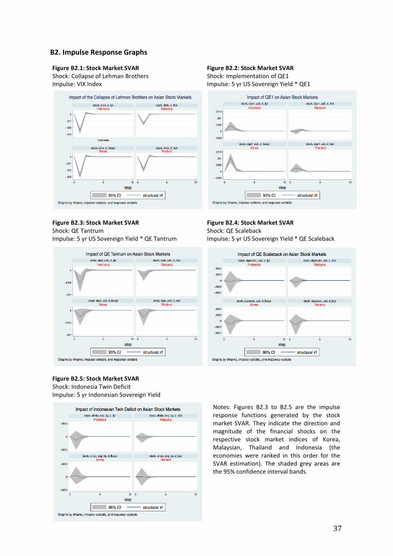
For the stock market SVAR, the impulse response charts in Figures B2.1, B2.2 and B2.3
show that the collapse of Lehman Brothers, implementation of QE1 and the QE
tantrum did lead to significant and similar directional responses in the Korean,
Malaysian, Thai and Indonesian equity markets. Nevertheless, while the impulse
response charts for the QE1 and QE tantrum shocks exhibited relatively wider 95%
confidence interval bands, the impact appears to be confined to mostly one-sided
effects. The impulse response charts for the QE scaleback and Indonesian twin deficit
shocks (Figures B2.4 and B2.5), however, reveal insignificant responses towards the
18
shocks given that the confidence intervals are wide and include both positive and
negative values. Therefore, these shocks will be excluded from Stage 2 onwards.
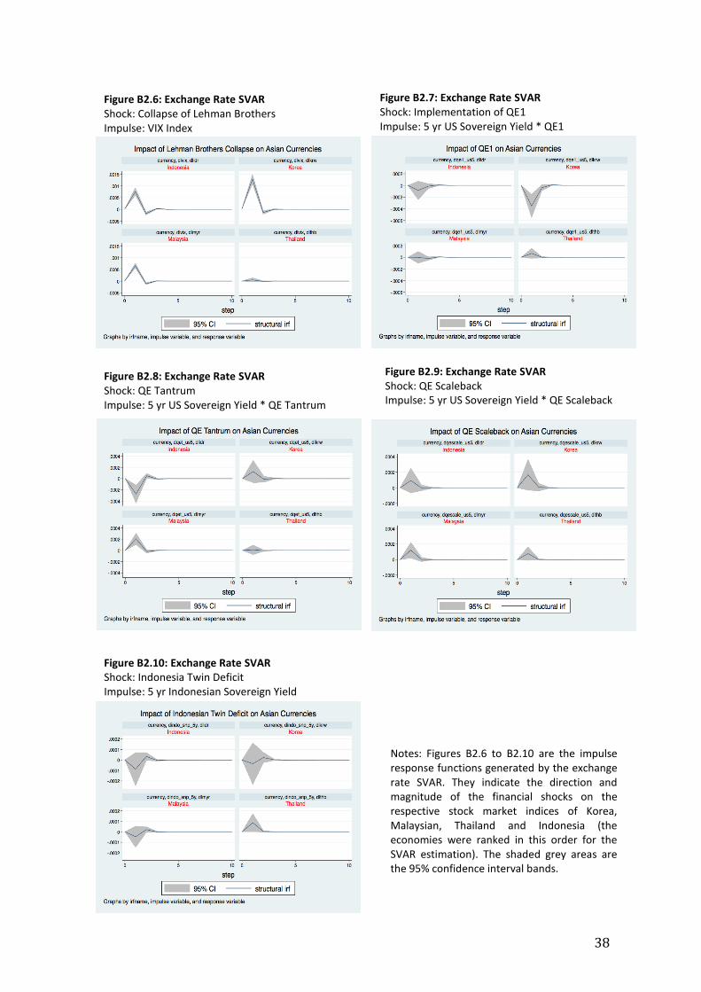
In terms of currency effects, the impulse response charts for the Lehman Brothers
shock (Figure B2.6) shows that all four currencies experienced significant depreciation.
For the impact of QE1, Figure B2.7 suggests that the rupiah, won and ringgit underwent
some appreciation, whereas the baht depreciated in response to this shock. While the
confidence band for the rupiah and ringgit may suggest some uncertainty in the
impact, this could be a reflection of exchange rate intervention during the period as the
region as a whole did experience strong capital inflows that are likely to have exerted
pressures on the exchange rate. The QE tantrum event did cause significant
appreciation in the rupiah, and depreciation in the won and ringgit. The baht did not
experience much discernible impact during this period, which may also have been a
consequence of exchange rate intervention to manage volatility at that time. Figure
B2.9 shows that the QE scaleback did have broadly significant depreciation effects on
all four currencies. Lastly, the Indonesian twin deficit shock appears to have lead to
appreciation in the rupiah, won and ringgit, and depreciation in the baht. The 95%
confidence bands for Indonesia, Malaysia and Thailand, are mostly one-sided, despite
being relatively wide. For Korea, however, the width of the confidence band covers
both positive and negative values. The effects for Korea may not be surprising as
investors may view Korea12 as different from the other three economies given that it
has experienced greater levels of economic development compared to the other three
12
The IMF presently categorizes Korea as an advanced economy, and Malaysia, Thailand and Indonesia as emerging and developing economies.
19
economies. Nevertheless, the next two stages will continue to consider these shocks as
the currency effects may be a reflection of central bank intervention to manage
volatility.
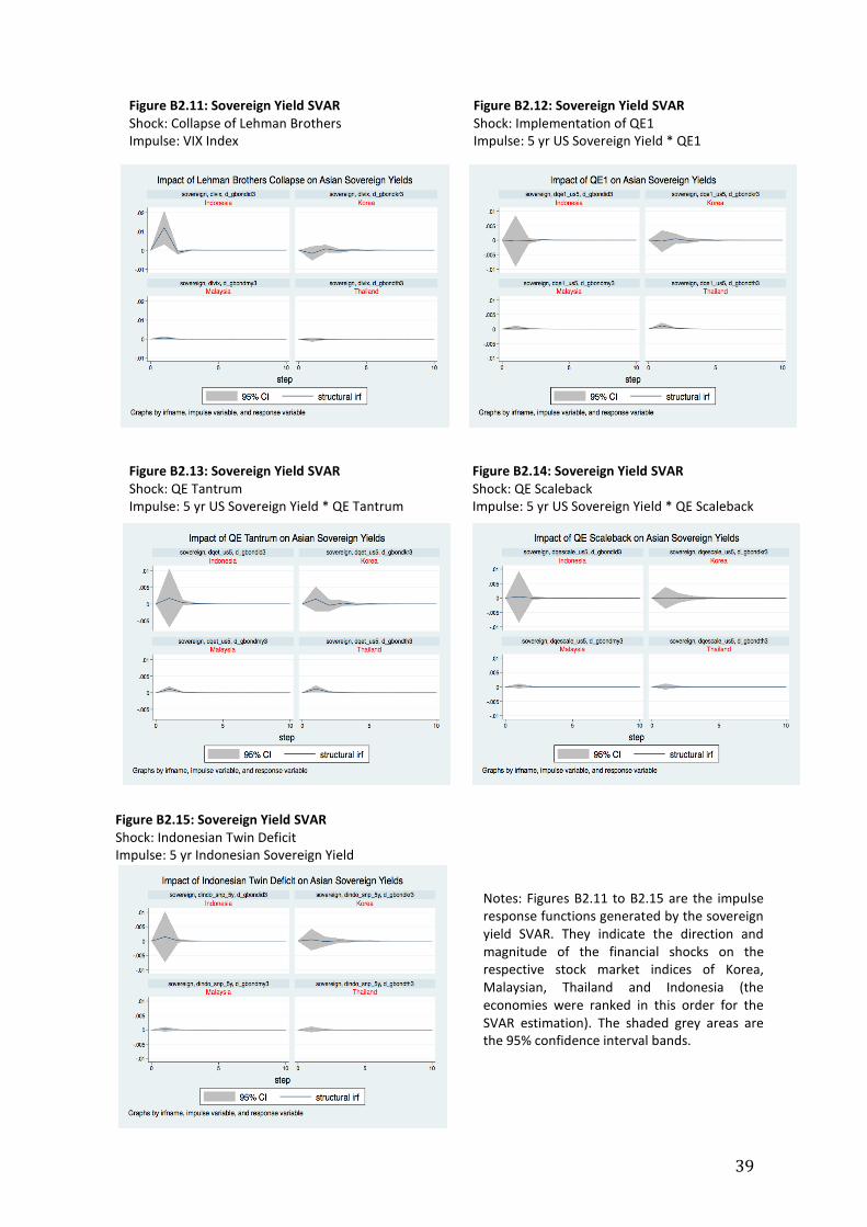
The sovereign yield SVAR strongly suggests that most of the global and regional
financial shocks that were tested did not have much visible impact to Asian sovereign
markets. Given these results, the next stage of estimations will focus only on contagion
effects in equity and currency markets. While the directional impact in the currency
market and the twin deficit concerns on stock markets may not be similar across
countries, the following empirical tests will continue to consider these shocks as the
trends may be due to differences in economic fundamentals and exchange rate
intervention. In any case, the next two stages of estimations will provide further
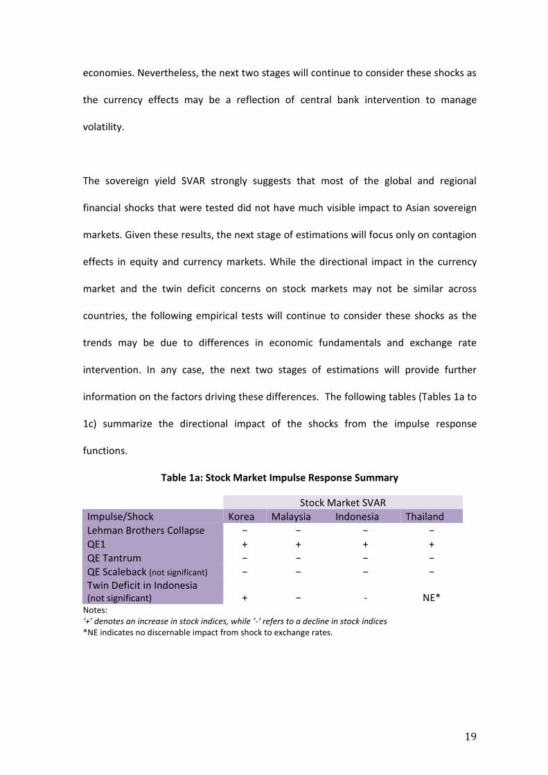
information on the factors driving these differences. The following tables (Tables 1a to
1c) summarize the directional impact of the shocks from the impulse response
functions.
Table 1a: Stock Market Impulse Response Summary
Stock Market SVAR Impulse/Shock Korea Malaysia Indonesia Thailand Lehman Brothers Collapse − − − − QE1 + + + + QE Tantrum − − − − QE Scaleback (not significant) − − − − Twin Deficit in Indonesia (not significant) + − - NE*
Notes: ‘+’ denotes an increase in stock indices, while ‘-‘ refers to a decline in stock indices *NE indicates no discernable impact from shock to exchange rates.
20
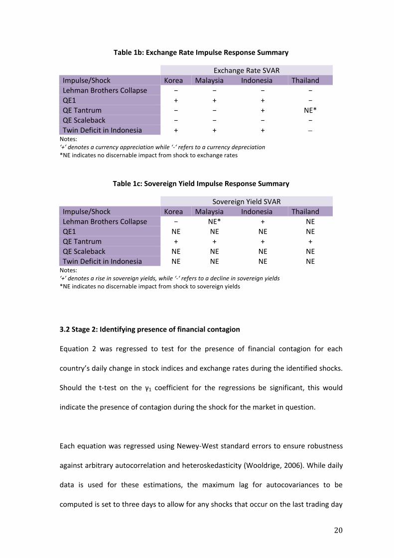
Table 1b: Exchange Rate Impulse Response Summary
Exchange Rate SVAR Impulse/Shock Korea Malaysia Indonesia Thailand Lehman Brothers Collapse − − − − QE1 + + + − QE Tantrum − − + NE* QE Scaleback − − − − Twin Deficit in Indonesia + + +
Notes: ‘+’ denotes a currency appreciation while ‘-‘ refers to a currency depreciation *NE indicates no discernable impact from shock to exchange rates
Table 1c: Sovereign Yield Impulse Response Summary
Sovereign Yield SVAR Impulse/Shock Korea Malaysia Indonesia Thailand
Lehman Brothers Collapse − NE* + NE QE1 NE NE NE NE QE Tantrum + + + + QE Scaleback NE NE NE NE
Twin Deficit in Indonesia NE NE NE NE Notes: ‘+’ denotes a rise in sovereign yields, while ‘-‘ refers to a decline in sovereign yields *NE indicates no discernable impact from shock to sovereign yields
3.2 Stage 2: Identifying presence of financial contagion
Equation 2 was regressed to test for the presence of financial contagion for each
country’s daily change in stock indices and exchange rates during the identified shocks.
Should the t-test on the γ1 coefficient for the regressions be significant, this would
indicate the presence of contagion during the shock for the market in question.
Each equation was regressed using Newey-West standard errors to ensure robustness
against arbitrary autocorrelation and heteroskedasticity (Wooldrige, 2006). While daily
data is used for these estimations, the maximum lag for autocovariances to be
computed is set to three days to allow for any shocks that occur on the last trading day
21
of the week, i.e. Friday, to be immediately transmitted on the first trading day of the
following work week, i.e. Monday.
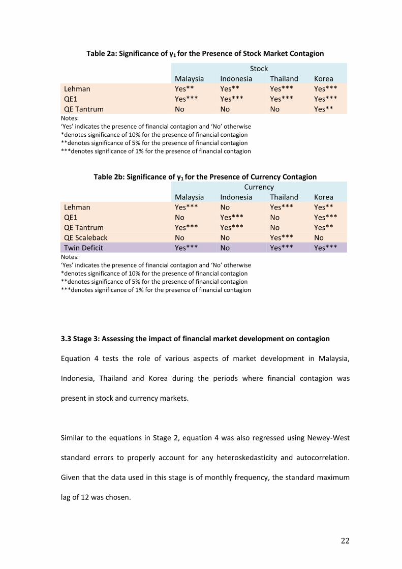
Tables 2a and 2b summarize the estimation results. There is evidence of significant
financial contagion for all four equity markets during the collapse of Lehman Brothers,
and implementation of QE1. With the exception of Korea, stock markets in Malaysia,
Indonesia and Thailand did not experience financial contagion during QE tantrum.
For currency markets, however, there appears to be no consistent impact of financial
contagion for all markets given the same shocks. For instance, during the Lehman
Brothers collapse and twin deficit concerns, all currencies showed signs of contagion
except for the rupiah. Given the noticeably strong contagion effects in the stock market
during these shocks, these results come as a surprise and strongly allude to the
presence of active currency intervention to mitigate the contagion effects. During the
implementation of QE1, only the rupiah and won can be categorized as having
experienced contagion. Contagion effects in the ringgit, rupiah and won were present
during the QE tantrum, and had disappeared by the time the scaleback was actually
implemented. One plausible reason for these developments is that market participants
had already priced in the effects of a scaleback during the tantrum period, resulting in
no change in the relationship between asset returns in the US and most Asian markets
when the QE scaleback was actually implemented.
22
Table 2a: Significance of γ1 for the Presence of Stock Market Contagion
Stock Malaysia Indonesia Thailand Korea Lehman Yes** Yes** Yes*** Yes*** QE1 Yes*** Yes*** Yes*** Yes*** QE Tantrum No No No Yes**
Notes: ‘Yes’ indicates the presence of financial contagion and ‘No’ otherwise *denotes significance of 10% for the presence of financial contagion **denotes significance of 5% for the presence of financial contagion ***denotes significance of 1% for the presence of financial contagion
Table 2b: Significance of γ1 for the Presence of Currency Contagion Currency Malaysia Indonesia Thailand Korea Lehman Yes*** No Yes*** Yes** QE1 No Yes*** No Yes*** QE Tantrum Yes*** Yes*** No Yes** QE Scaleback No No Yes*** No Twin Deficit Yes*** No Yes*** Yes***
Notes: ‘Yes’ indicates the presence of financial contagion and ‘No’ otherwise *denotes significance of 10% for the presence of financial contagion **denotes significance of 5% for the presence of financial contagion ***denotes significance of 1% for the presence of financial contagion
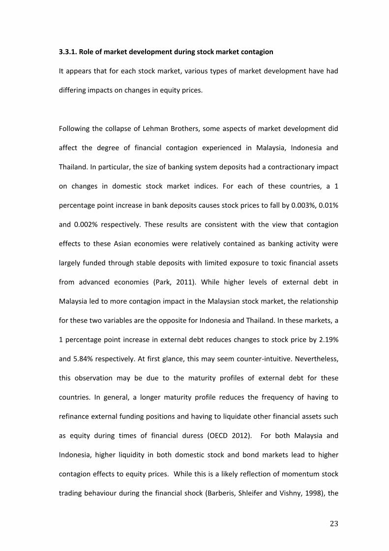
3.3 Stage 3: Assessing the impact of financial market development on contagion
Equation 4 tests the role of various aspects of market development in Malaysia,
Indonesia, Thailand and Korea during the periods where financial contagion was
present in stock and currency markets.
Similar to the equations in Stage 2, equation 4 was also regressed using Newey-West
standard errors to properly account for any heteroskedasticity and autocorrelation.
Given that the data used in this stage is of monthly frequency, the standard maximum
lag of 12 was chosen.
23
3.3.1. Role of market development during stock market contagion
It appears that for each stock market, various types of market development have had
differing impacts on changes in equity prices.
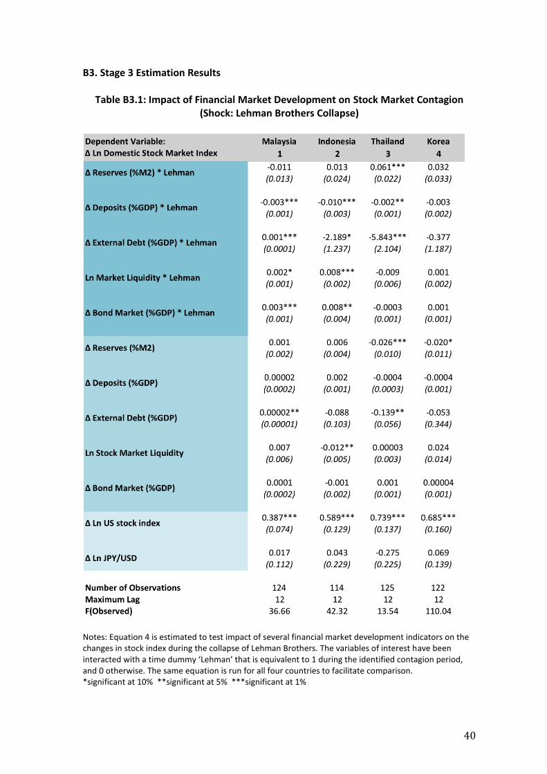
Following the collapse of Lehman Brothers, some aspects of market development did
affect the degree of financial contagion experienced in Malaysia, Indonesia and
Thailand. In particular, the size of banking system deposits had a contractionary impact
on changes in domestic stock market indices. For each of these countries, a 1
percentage point increase in bank deposits causes stock prices to fall by 0.003%, 0.01%
and 0.002% respectively. These results are consistent with the view that contagion
effects to these Asian economies were relatively contained as banking activity were
largely funded through stable deposits with limited exposure to toxic financial assets
from advanced economies (Park, 2011). While higher levels of external debt in
Malaysia led to more contagion impact in the Malaysian stock market, the relationship
for these two variables are the opposite for Indonesia and Thailand. In these markets, a
1 percentage point increase in external debt reduces changes to stock price by 2.19%
and 5.84% respectively. At first glance, this may seem counter-intuitive. Nevertheless,
this observation may be due to the maturity profiles of external debt for these
countries. In general, a longer maturity profile reduces the frequency of having to
refinance external funding positions and having to liquidate other financial assets such
as equity during times of financial duress (OECD 2012). For both Malaysia and
Indonesia, higher liquidity in both domestic stock and bond markets lead to higher
contagion effects to equity prices. While this is a likely reflection of momentum stock
trading behaviour during the financial shock (Barberis, Shleifer and Vishny, 1998), the
24
small coefficients on these variables may be due to negative feedback trading, where
domestic market participants take the opportunity from an equity sell-off to purchase
stock at cheaper prices, thus reducing any one-sided pressure in stock markets. It is
interesting to note that during this shock, market development indicators had no
significant impact on stock price changes in Korea. (Appendix B3, Table B3.1)
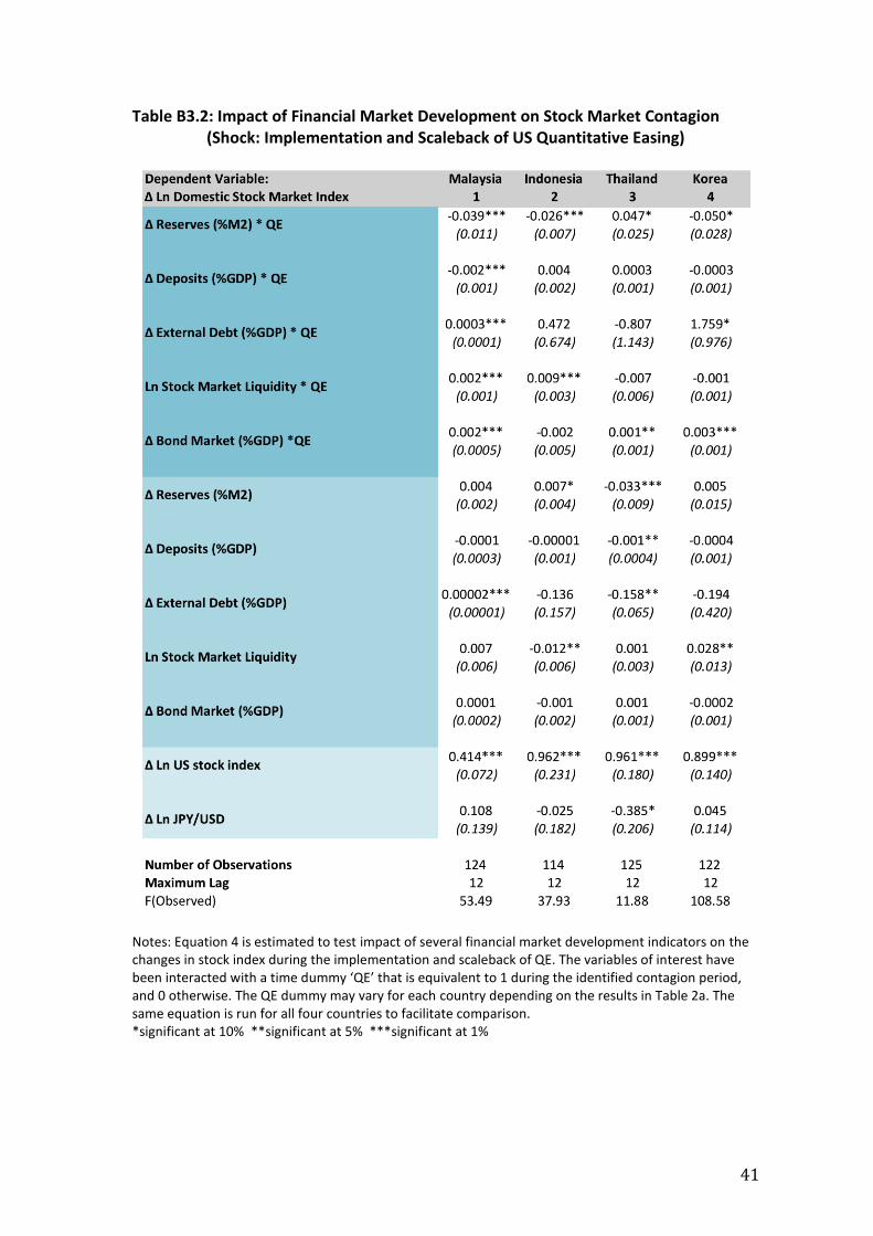
During the implementation and scaleback of QE13, the level of central bank reserves, in
particular, had significant impact on stock market contagion across all four economies.
A 1 percentage point rise in international reserves has the ability to reduce changes in
stock prices by 0.04%, 0.03% and 0.05% for Malaysia, Indonesia and Korea respectively.
Central bank intervention to manage exchange rate volatility (indirectly) works to
reduce the risk of currency mismatches for foreign investors, and domestic traders with
international portfolios, thereby reducing equity sell-off pressures. For Thailand,
however, the impact of higher reserve levels contributes to stronger changes in stock
prices. The impacts of other aspects of market development for Malaysia were
significant and of similar signs as during the Lehman shock. During the QE related
financial shock, external debt was a contributing factor to stock market contagion in
Korea. A 1 percentage point increase in external debt increases stock price changes by
1.76%. Similar to the estimations during the Lehman shock, higher capital market
liquidity led to significant but small changes in stock prices across all four economies.
(Appendix B3, Table B3.2)
13
To ensure consistency with Stage 2 results for the QE related shocks, the time dummy on the interaction terms only account for the period in which QE1 was introduced, except for Korea, whose time dummy also captures the impact of QE tantrum.
25
For all estimations on stock market contagion, changes in US stock prices have had
significant and amplifying effects to financial contagion in these Asian economies. The
impact of developments in Japanese yen was, however, not significant in all instances.
3.3.2 Role of market development during currency contagion
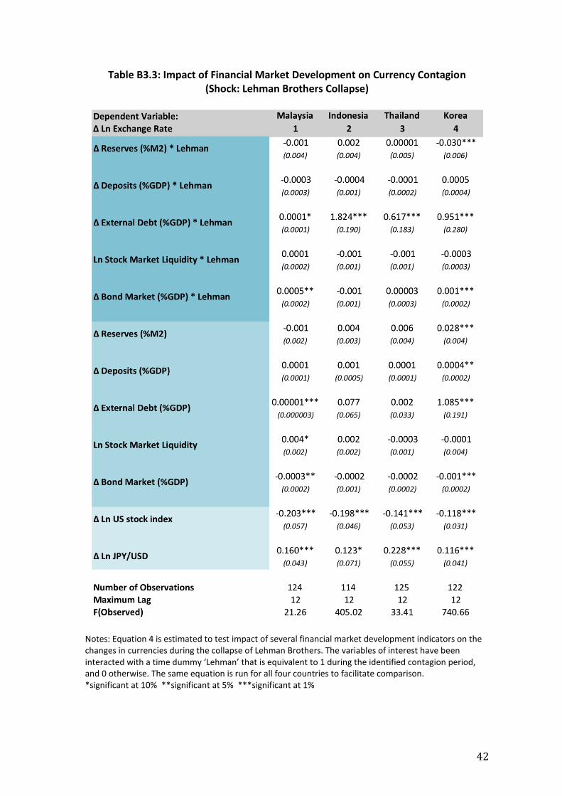
During the Lehman shock, all four currencies underwent initial depreciation due to
capital flight in an environment of heightened global risk aversion. Overall, only
international reserves in Korea had the effect of offsetting depreciating pressure during
this period; depreciation pressure in the Korean won was reduced by 0.03% for every 1
percentage point increase in reserves. The stock of external debt contributed to
depreciation pressure across all four currencies. In particular, a 1 percentage point
increase in external debt resulted in currency depreciations of 0.0001%, 1.82%, 0.62%
and 0.95% for the Malaysian ringgit, Indonesian rupiah, Thai baht and Korean won
respectively. Bond market size and liquidity, while significant for Malaysia and Korea,
had muted effects in amplifying currency depreciation during the Lehman shock.
(Appendix B3, Table B3.3)
Throughout the implementation and scaleback of QE14, the impact of external debt and
banking system deposits were significant across all currencies. A 1 percentage point
increase in external debt resulted in 1.36%, 0.55% and 1.20% additional depreciation in
the rupiah, baht and won, while the impact on the ringgit was offset by a 0.002%
appreciation. Stronger levels of banking system deposits had the effect of adding some
14
Analysis of the impact of QE on currency contagion will be kept general as the implementation of QE mostly resulted in appreciation pressure, while the scaleback in QE had on average resulted in depreciation in Asian currencies.
26
appreciation pressure on the currencies, except for Indonesia. From this perspective
and owing to the fact that the region experienced strong capital inflows throughout the
implementation of QE15, the impact of deposit levels may differ among countries and
depend largely upon holder and type of deposit composition and central bank liquidity
management strategies. In addition, the level of adequate international reserves was
also effective in reducing currency contagion in the baht and won during the period; a 1
percentage point increase in reserves during the period led to a 0.01% and 0.03%
reduction in changes to the exchange rate. In terms of capital market liquidity, larger
bond markets in Thailand and Korea likely contributed to further depreciation pressure
to their respective local currencies, while the opposite is true for Indonesia. For
Malaysia, the level of stock market liquidity mattered more for offsetting any
appreciation pressure on the ringgit. The coefficients on these variables are very small,
rendering only significant but small effects on currency contagion. (Appendix B3, Table
B3.4)
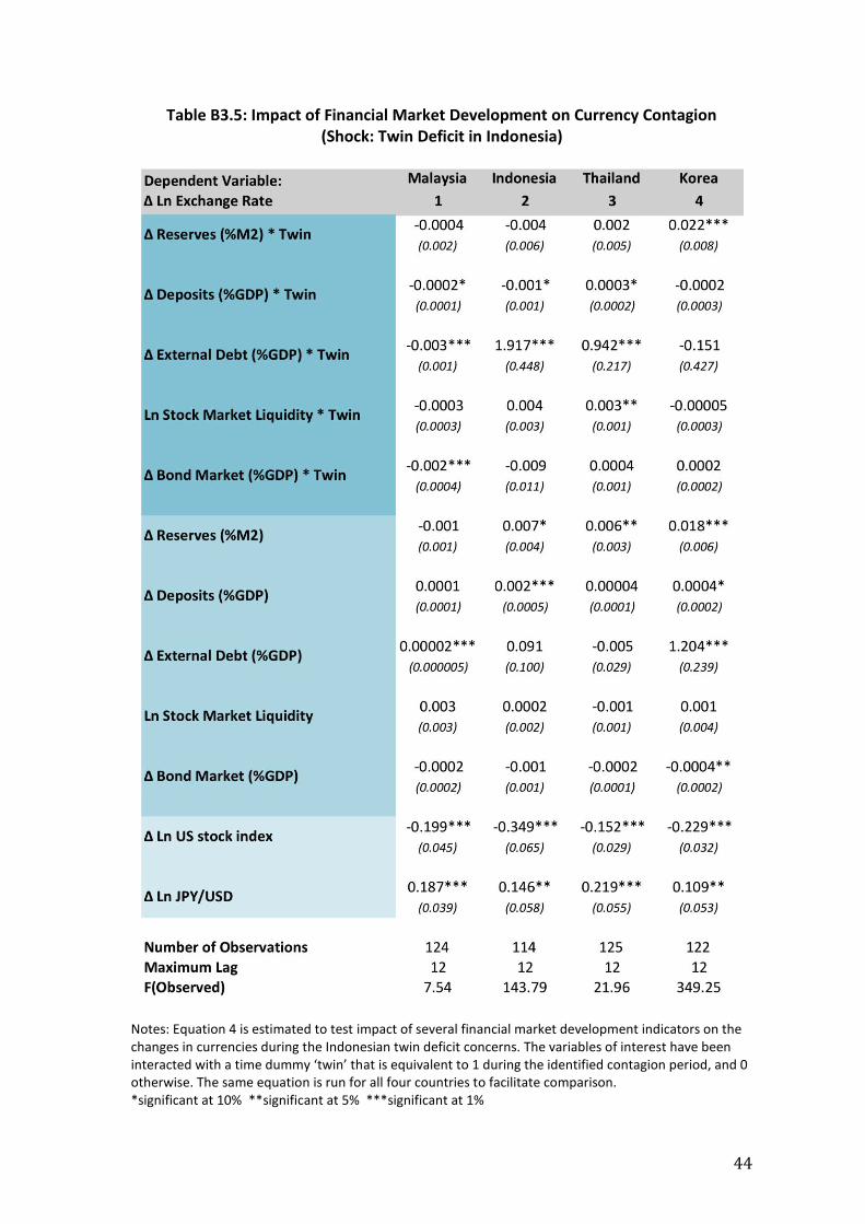
During the occurrence of the Indonesian twin deficit16, the level of banking system
deposits had significant but small effects on currency contagion. The role of external
debt, i.e. the extent of financial openness, however, did contribute to further
depreciation in the rupiah and baht during the period. Alternatively, for Malaysia, the
level of external debt had an offsetting effect on the changes in the ringgit. Capital
15
The impact of the scaleback in QE on the currency should be influenced by the extent of capital inflows experienced during the prior implementation of QE. Also, to ensure consistency with Stage 2 results for the QE related shocks, the time dummy in the interaction terms for each country only reflects their respective significant contagion events; i.e. QE1, QE tantrum, QE scaleback, or the relevant combinations. 16
Indonesia continues to remain in twin deficit but efforts by the Government and monetary authorities have thus far eased investor concerns, as evidenced by the upgrade in S&P’s rating outlook for Indonesia from negative to stable in May 2014.
27
market liquidity appears to only matter for Thailand and Malaysia; a 1 percentage point
increase in stock market activity resulted in a 0.003% depreciation in the baht while a 1
percentage point rise in the size of local currency bond market in Malaysia would have
resulted in a 0.002% appreciation in the ringgit. The coefficients on these variables are
very small, rendering only significant but small effects on currency contagion. Similar to
previous shocks, the sizes of the coefficients suggest minimal impact. (Appendix B3,
Table B3.5)
Throughout these estimations, the impact of changes in the US stock market on the
currency was significant and negative; implying that any increase in the US stock prices
would have led to appreciation pressure in the exchange rates. The impact of shifts in
the value of the Japanese yen however, is significant and positive on most Asian
currencies during each shock tested.
3.3.3 Simulating a stronger regional shock
Throughout the sample period of this study, i.e. from 2005 to 2015, there have not
been any major financial shocks emanating from within the Asian region that can be
compared to the shocks experienced during the Asian Financial Crisis (AFC). It would
thus be interesting to test whether present levels of market development would have
alleviated the extent of financial contagion back then. To do so, the dependent
variables i.e. changes in stock indices and currency from 2005 to 2015 are replaced
with the same variables for the period 1990 to 2000 to simulate the same degree of
shocks. The same estimation is re-run, and similar to the previous regressions, we
28
examine the impact of present levels market development on the AFC simulated scale
of contagion.
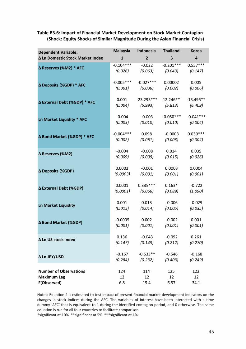
For similar levels of stock market contagion during the AFC, present levels of market
development are likely to play a stronger offsetting role in minimizing changes to
equity prices when compared to the previously tested shocks in this paper. The most
notable impact is the level of external debt, whereby a 1 percentage point increase in
this factor will reduce changes to stock prices by 23.3% and 13.5% in Indonesia and
Korea, but increase contagion in Thailand by 12.3%. These results strongly suggest that
present compositions of external debt, particularly in Indonesia and Korea, are of a
sustainable nature and could work in favour of cushioning stock market contagion in
the event of a massive financial shock from within the region. The build-up of adequate
reserves since the AFC for Malaysia and Thailand will also be able to offset the
simulated shock. In addition, a comparatively stronger and more robust banking system
in both Malaysia and Indonesia would also work to contain the simulated shocks in the
equity market. Given that banking systems in these economies are no longer reliant on
external short-term funding to fund their business, the build-up of a stable deposit
base has made the financial system more resilient against financial shocks. The increase
in stock market liquidity in Thailand and Korea, and size of bond market in Malaysia
should also play an offsetting role in managing stock market contagion. (Appendix B3,
Table B3.6)
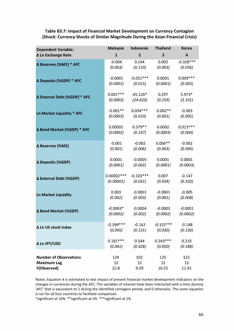
The impact of financial market development on currency contagion appears to be
mixed across the four economies. The level of reserves only has a significant impact in
29
offsetting depreciation pressure in Korea; a 1 percentage point increase in adequate
reserves reduces changes in the won by 0.33%. A stronger deposit base, however, only
has a significant offsetting impact for the rupiah, while this factor could further
aggravate changes in the won. In terms of financial openness, while a 1 percentage
point increase in external debt reduces currency contagion by 45.1% for Indonesia, it
would amplify changes in the won by 6.0%. Greater stock market liquidity today will
help contain currency contagion pressures in the ringgit and baht, but could worsen
conditions for the rupiah. The size of current bond markets would also exacerbate
depreciation pressures during shocks of similar magnitude during the AFC in Indonesia
and Korea. (Appendix B3, Table B3.7)
4.0 Conclusion and policy recommendations
The estimation results broadly suggest that financial market development undertaken
post-AFC have played significant roles in the management of financial contagion for the
Asian economies in this study.
Since the 2008 GFC, stock market contagion arising from global shocks have been
mostly offset by stronger levels of banking system deposits. This comes as no surprise
as deposits provide a more stable funding base for banks, creating insulation from
adverse external financial shocks. Greater financial openness as reflected by external
debt (normalised to GDP) also served to reduce stock market contagion, especially
Indonesia and Thailand. This strongly suggests that external debt composition in terms
of maturity profiles and debt holders matter in ensuring that financial openness works
to contain, rather than exacerbate stock market contagion. Interestingly, greater equity
30
and bond market liquidity could intensify changes in stock prices. This could, however,
be a reflection of momentum stock trading behaviour during financial duress.
Nevertheless, the small coefficients on these factors may be driven by traders
offsetting massive sell-off pressures by taking the opportunity to purchase certain
stocks with the view the shock is likely to be temporary.
In terms of exchange rate markets, the various aspects of financial market contagion do
not seem to overwhelmingly offset currency contagion. Higher levels of external debt
raise the risk of aggravating contagion, while the impact of stronger capital market
liquidity and banking system deposits appear mixed. On balance, however, higher
levels of adequate reserves do work to significantly offset currency contagion
depending on the type of shock.
To provide a clearer answer to whether there are differences in the ability of current
Asian financial systems to withstand global and regional shocks, this study simulates
the magnitude of equity and currency shocks experienced by these countries during
the AFC and test whether present levels of market development would have been able
to offset the adverse impact. Financial market development in this context has on
average, stronger offsetting effects on stock market contagion compared to the
currency market. This shows that should there be a strong shock from within the region
again, the exchange rates are likely to transmit stronger contagion effects to the
economy relative to the equity market. This may not necessarily be a surprising result,
as these Asian economies have worked towards greater flexibility in their exchange
31
rate regimes since the AFC, with intervention occurring to manage the volatility rather
than the absolute level of the exchange rate.
These results show that while progress has been made in terms of carefully sequenced
financial market development, there remains room for improvement. In particular,
policy makers may need to re-look at the details of their capital market liquidity. For
instance, in some economies there could be disproportionate concentration of either
domestic or foreign ownership of certain financial assets, causing varying degrees of
effectiveness in managing financial contagion. Nevertheless, it could also be the case
that policymakers have sought a more cautious approach to market development.
While the creation of certain financial instruments, such as central bank bills, is
intended to manage market liquidity more efficiently, it could simultaneously act as a
conduit for potentially destabilizing speculative activity via the offshore derivatives
market. In terms of market participation, while the presence of a few institutional
investors can provide the stability needed during periods of financial contagion, this
may not necessarily add to market vibrance during ‘normal’ conditions.
Going forward, further advancements to this study can be done to examine the impact
of other aspects of market development, especially the role of a growing derivatives
market and active central bank liquidity management. In quantifying the effectiveness
of market development on managing financial contagion, it could also be worthwhile to
consider further country-specific details in the empirical analysis.
32
References
Baig, Taimur and Goldfajn, Ilan, (1999) “Financial Market Contagion in the Asian Crisis”
IMF Staff Papers, Vol 46, No 2, June.
Barberis, Nicholas., Shleifer, Andrei., and Vishny, Robert, 1998, “A Model of Investor
Sentiment” Journal of Financial Economics 49, pages 307-343, February.
Boot, Arnold W.A. and Thakor, Anjan V., 1997, “Financial System Architecture” The
Review of Financial Studies, Vol. 10, No. 3, pages 693-733, Autumn.
Botman, Dennis P.J, de Carvalho Filho, Irineu and lam, Raphael W., 2013, “The Curious
Case of the Yen as a Safe Haven Currency: A Forensic Analysis”, IMF Working Papers,
No 13/228, November.
Chami, Ralph., Sharma, Sunil and Fullenkamp, Connel, 2009, “A Framework for
Financial Market Development” Journal of Economic Policy Reform, Taylor & Francis
Journals, Vol 13(2), pages 107-135.
Demirgüç-Kunt, Asli., Feyen, Erik., and Levine, Ross., 2012. “The Evolving Importance of
Banks and Securities Markets” The World Bank Economic Review, pages 1-15, August.
Devereux, Michael B. and Yetman, James, 2010, “Financial Contagion and Vulnerability
of Asian Financial Markets”, Bank of International Settlements Asian Office Research,
June
Dornbusch, Rudiger., Chui Park, Yung., and Claessens, Stijn., 2000 “Contagion:
Understanding How It Spreads”, The World Bank Research Observer, Vol 15, No 2, page
177-197, August.
33
Dungey,M., Fry, Renée., González-Hermosillo, Brenda and Martin, Vance, 2003,
“Characterizing Global Investors’ Risk Appetite for Emerging Market Debt During
Financial Crises”, IMF Working Paper, Working Paper No 03/251, December.
Dungey, Mardi., Fry, Renée., González-Hermosillo, Brenda and Martin, Vance, 2005,
“Empirical Modelling of Contagion: A Review of Methodologies” Quantitative Finance,
Taylor & Francis Journals, Vol 5(1), pages 9-24
Financial Sector Assessment: A Handbook, Chapter 2, Indicators of Financial Structure,
Development and Soundness, 2005, World Bank and International Monetary Fund.
Forbes, Kristin and Rigobon, Roberto, 1998, “Measuring Stock Market Contagion:
Conceptual Issues and Empirical Tests” Mimeograph, Massachusetts Institute of
Technology, April.
Fornari, Fabio and Stracca, Livio. 2013. “What does a Financial Shock do? First
International Evidence”, Working Paper Series 1522, European Central Bank.
Lindgren, Carl-Johan., Baliño, Tomás J.T., Enoch, Charles., Gulde, Anne-Marie., Quintyn,
Marc. and Teo, Leslie. 1999. “Financial Sector Crisis and Restructuring Lessons from
Asia” Occasional Paper 188, IMF Washington DC
OECD 2012, “Financial Contagion in the Era of Globalised Banking” OECD Economics
Department Policy Notes, No. 14, June.
Obstfeld, Maurice. 2009. “International Finance and Growth in Developing Countries:
What Have We Learned?” IMF Staff Papers, Palgrave Macmillan Journals, vol. 56(1),
pages 63-111, April.
Ozkan, F. Gulcin and Unsal, D. Filiz, 2012 “Global Financial Crisis, Financial Contagion and Emerging Markets” IMF Working Paper, Working Paper No. 12/293, December.
34
Park, Cyn-Young. 2011. “Asian Financial System: Development and Challenges” ADB
Economics Working Paper Series, No. 285, November.
International Organisation of Supreme Audit Institutions (INTOSAI) Taskforce Subgroup
1, 2010, “The Causes of the Global Financial Crisis and Their Implications for Supreme
Audit Institutions” International Organisation of Supreme Audit Institutions (INTOSAI)
Weinstein, David E. and Yafeh, Yishay, 1998, “On the Costs of a Bank-Centered
Financial System: Evidence from the Changing Main Bank Relations in Japan” Journal of
Finance, Vol 53, pages 635-672, April.
Whaley, Robert E. 2008, “Understanding VIX” SSRN Electronic Journal, 11/2008
Wooldridge, Jeffrey M. 2006, “Introductory Econometrics: A Modern Approach”
Chapter 12: Serial Correlation and Heteroskedaticity in Time Series Regressions, 3RD
Edition, Thomson South-Western.
35
Appendix A: Empirical Strategy
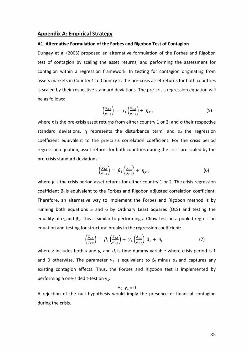
A1. Alternative Formulation of the Forbes and Rigobon Test of Contagion
Dungey et al (2005) proposed an alternative formulation of the Forbes and Rigobon
test of contagion by scaling the asset returns, and performing the assessment for
contagion within a regression framework. In testing for contagion originating from
assets markets in Country 1 to Country 2, the pre-crisis asset returns for both countries
is scaled by their respective standard deviations. The pre-crisis regression equation will
be as follows:
(𝑥2,𝑡
𝜎𝑥,2) = 𝛼1 (
𝑥1,𝑡
𝜎𝑥,1) + 𝜂𝑥,𝑡 (5)
where x is the pre-crisis asset returns from either country 1 or 2, and σ their respective
standard deviations. η represents the disturbance term, and α1 the regression
coefficient equivalent to the pre-crisis correlation coefficient. For the crisis period
regression equation, asset returns for both countries during the crisis are scaled by the
pre-crisis standard deviations:
(𝑦2,𝑡
𝜎𝑥,2) = 𝛽1 (
𝑦1,𝑡
𝜎𝑥,1) + 𝜂𝑦,𝑡 (6)
where y is the crisis period asset returns for either country 1 or 2. The crisis regression
coefficient β1 is equivalent to the Forbes and Rigobon adjusted correlation coefficient.
Therefore, an alternative way to implement the Forbes and Rigobon method is by
running both equations 5 and 6 by Ordinary Least Squares (OLS) and testing the
equality of α1 and β1. This is similar to performing a Chow test on a pooled regression
equation and testing for structural breaks in the regression coefficient:
(𝑍2,𝑡
𝜎𝑥,2) = 𝛽1 (
𝑍1,𝑡
𝜎𝑥,1) + 𝛾1 (
𝑍1,𝑡
𝜎𝑥,𝑡) 𝑑𝑡 + 𝜂𝑡 (7)
where z includes both x and y, and d1 is time dummy variable where crisis period is 1
and 0 otherwise. The parameter γ1 is equivalent to β1 minus α1 and captures any
existing contagion effects. Thus, the Forbes and Rigobon test is implemented by
performing a one-sided t-test on γ1:
H0: γ1 = 0 A rejection of the null hypothesis would imply the presence of financial contagion
during the crisis.
36
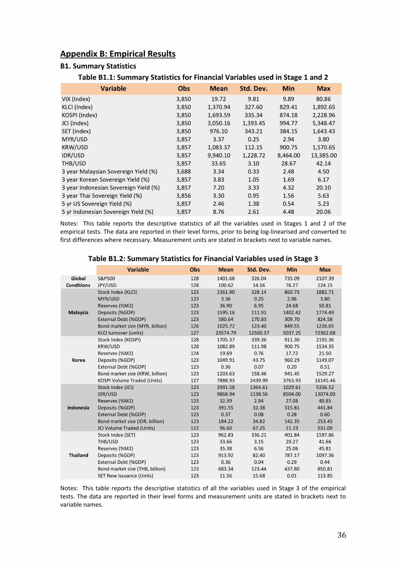
Appendix B: Empirical Results
B1. Summary Statistics
Table B1.1: Summary Statistics for Financial Variables used in Stage 1 and 2
Notes: This table reports the descriptive statistics of all the variables used in Stages 1 and 2 of the empirical tests. The data are reported in their level forms, prior to being log-linearised and converted to first differences where necessary. Measurement units are stated in brackets next to variable names.
Table B1.2: Summary Statistics for Financial Variables used in Stage 3
Notes: This table reports the descriptive statistics of all the variables used in Stage 3 of the empirical tests. The data are reported in their level forms and measurement units are stated in brackets next to variable names.
37
B2. Impulse Response Graphs
Figure B2.1: Stock Market SVAR Shock: Collapse of Lehman Brothers Impulse: VIX Index
Figure B2.2: Stock Market SVAR Shock: Implementation of QE1 Impulse: 5 yr US Sovereign Yield * QE1
Figure B2.3: Stock Market SVAR Shock: QE Tantrum Impulse: 5 yr US Sovereign Yield * QE Tantrum
Figure B2.4: Stock Market SVAR Shock: QE Scaleback Impulse: 5 yr US Sovereign Yield * QE Scaleback
Figure B2.5: Stock Market SVAR Shock: Indonesia Twin Deficit Impulse: 5 yr Indonesian Sovereign Yield
Notes: Figures B2.3 to B2.5 are the impulse response functions generated by the stock market SVAR. They indicate the direction and magnitude of the financial shocks on the respective stock market indices of Korea, Malaysian, Thailand and Indonesia (the economies were ranked in this order for the SVAR estimation). The shaded grey areas are the 95% confidence interval bands.
38
Figure B2.6: Exchange Rate SVAR Shock: Collapse of Lehman Brothers Impulse: VIX Index
Figure B2.7: Exchange Rate SVAR Shock: Implementation of QE1 Impulse: 5 yr US Sovereign Yield * QE1
Figure B2.8: Exchange Rate SVAR Shock: QE Tantrum Impulse: 5 yr US Sovereign Yield * QE Tantrum
Figure B2.9: Exchange Rate SVAR Shock: QE Scaleback Impulse: 5 yr US Sovereign Yield * QE Scaleback
Figure B2.10: Exchange Rate SVAR Shock: Indonesia Twin Deficit Impulse: 5 yr Indonesian Sovereign Yield
Notes: Figures B2.6 to B2.10 are the impulse response functions generated by the exchange rate SVAR. They indicate the direction and magnitude of the financial shocks on the respective stock market indices of Korea, Malaysian, Thailand and Indonesia (the economies were ranked in this order for the SVAR estimation). The shaded grey areas are the 95% confidence interval bands.
39
B3. Stage 3 Estimation Results
Figure B2.11: Sovereign Yield SVAR Shock: Collapse of Lehman Brothers Impulse: VIX Index
Figure B2.12: Sovereign Yield SVAR Shock: Implementation of QE1 Impulse: 5 yr US Sovereign Yield * QE1
Figure B2.13: Sovereign Yield SVAR Shock: QE Tantrum Impulse: 5 yr US Sovereign Yield * QE Tantrum
Figure B2.14: Sovereign Yield SVAR Shock: QE Scaleback Impulse: 5 yr US Sovereign Yield * QE Scaleback
Figure B2.15: Sovereign Yield SVAR Shock: Indonesian Twin Deficit Impulse: 5 yr Indonesian Sovereign Yield
Notes: Figures B2.11 to B2.15 are the impulse response functions generated by the sovereign yield SVAR. They indicate the direction and magnitude of the financial shocks on the respective stock market indices of Korea, Malaysian, Thailand and Indonesia (the economies were ranked in this order for the SVAR estimation). The shaded grey areas are the 95% confidence interval bands.
40
B3. Stage 3 Estimation Results
Table B3.1: Impact of Financial Market Development on Stock Market Contagion (Shock: Lehman Brothers Collapse)
Notes: Equation 4 is estimated to test impact of several financial market development indicators on the changes in stock index during the collapse of Lehman Brothers. The variables of interest have been interacted with a time dummy ‘Lehman’ that is equivalent to 1 during the identified contagion period, and 0 otherwise. The same equation is run for all four countries to facilitate comparison. *significant at 10% **significant at 5% ***significant at 1%
41
Table B3.2: Impact of Financial Market Development on Stock Market Contagion (Shock: Implementation and Scaleback of US Quantitative Easing)
Notes: Equation 4 is estimated to test impact of several financial market development indicators on the changes in stock index during the implementation and scaleback of QE. The variables of interest have been interacted with a time dummy ‘QE’ that is equivalent to 1 during the identified contagion period, and 0 otherwise. The QE dummy may vary for each country depending on the results in Table 2a. The same equation is run for all four countries to facilitate comparison. *significant at 10% **significant at 5% ***significant at 1%
42
Table B3.3: Impact of Financial Market Development on Currency Contagion (Shock: Lehman Brothers Collapse)
Notes: Equation 4 is estimated to test impact of several financial market development indicators on the changes in currencies during the collapse of Lehman Brothers. The variables of interest have been interacted with a time dummy ‘Lehman’ that is equivalent to 1 during the identified contagion period, and 0 otherwise. The same equation is run for all four countries to facilitate comparison. *significant at 10% **significant at 5% ***significant at 1%

43
Table B3.4: Impact of Financial Market Development on Currency Contagion (Shock: Implementation and Scaleback of US Quantitative Easing)
Notes: Equation 4 is estimated to test impact of several financial market development indicators on the changes in currencies during the implementation and scaleback of QE. The variables of interest have been interacted with a time dummy ‘QE’ that is equivalent to 1 during the identified contagion period, and 0 otherwise. The QE dummy may vary for each country depending on the results in Table 2b. The same equation is run for all four countries to facilitate comparison. *significant at 10% **significant at 5% ***significant at 1%
44
Table B3.5: Impact of Financial Market Development on Currency Contagion (Shock: Twin Deficit in Indonesia)
Notes: Equation 4 is estimated to test impact of several financial market development indicators on the changes in currencies during the Indonesian twin deficit concerns. The variables of interest have been interacted with a time dummy ‘twin’ that is equivalent to 1 during the identified contagion period, and 0 otherwise. The same equation is run for all four countries to facilitate comparison. *significant at 10% **significant at 5% ***significant at 1%
45
Table B3.6: Impact of Financial Market Development on Stock Market Contagion (Shock: Equity Shocks of Similar Magnitude During the Asian Financial Crisis)
Notes: Equation 4 is estimated to test impact of present financial market development indicators on the changes in stock indices during the AFC. The variables of interest have been interacted with a time dummy ‘AFC’ that is equivalent to 1 during the identified contagion period, and 0 otherwise. The same equation is run for all four countries to facilitate comparison. *significant at 10% **significant at 5% ***significant at 1%
46
Table B3.7: Impact of Financial Market Development on Currency Contagion (Shock: Currency Shocks of Similar Magnitude During the Asian Financial Crisis)
Notes: Equation 4 is estimated to test impact of present financial market development indicators on the changes in currencies during the AFC. The variables of interest have been interacted with a time dummy ‘AFC’ that is equivalent to 1 during the identified contagion period, and 0 otherwise. The same equation is run for all four countries to facilitate comparison. *significant at 10% **significant at 5% ***significant at 1%