THE REALITY GAP OF AUTONOMOUS UNDERWATER VEHICLE MAKO AND ...robotics.ee.uwa.edu.au/theses/2008-AUV-Dittmar.pdf · THE REALITY GAP OF AUTONOMOUS UNDERWATER VEHICLE MAKO AND SUBSIM

THE REALITY GAP OF

AUTONOMOUS UNDERWATER VEHICLE

MAKO AND SUBSIM

Markus DittmarDiplomarbeit Informatik (FH) 2008

Fachbereich Mathematik, Naturwissenschaften und Informatik,

Schwerpunkt Technisch-Wissenschaftliche Anwendungen,

FH-Gießen-Friedberg, Germany

Mobile Robotics Laboratory, Centre for Intelligent Information Processing

Systems, School of Electrical, Electronic and Computer Engineering,

The University of Western Australia.

Supervisor Professor Dr. Wust

Co-Supervisor A. Professor Thomas Braunl

Hiermit versichere ich, die vorliegende Arbeit selbststandig und unter ausschließlicher Ver-wendung der angegebenen Literatur und Hilfsmittel erstellt zu haben. Die Arbeit wurdebisher in gleicher oder ahnlicher Form keiner anderen Prufungsbehorde vorgelegt und auchnicht veroffentlicht.

Perth, den 30. November 2008

Markus Dittmar

Acknowledgements

It has been a great challenge for me to work on two projects within in my thesis. Thereare a number of people I want to mention and thank for their help and support. Makois a two-man project and without their help it would have been impossible to accomplishthis thesis.

Firstly, I want to thank my friend Stephan Beisken. He spent many of his free sundaysduring the winter with me at the pool and most of the time in the pool. At least with hotchocolate and coffee I could keep him alive successfully.

Many thanks goes to the gentlemen in the mechanical and electronic workshops. With-out their dedication and ideas many experimental setups would have been impossible.

I would like to give thanks to Thomas Braunl for giving me the opportunity to conductmy final project at the University of Western Australia. It has been amazing to “play”with the robots from the lab.

Last but not least I want to express my thank to Adrian Boeing for his guidance andsupport with PAL.

i

Contents

1 Introduction 1

1.1 Autonomous Underwater Vehicle . . . . . . . . . . . . . . . . . . . . . . . . 11.2 Motivation Mako . . . . . . . . . . . . . . . . . . . . . . . . . . . . . . . . . 11.3 Motivation SubSim . . . . . . . . . . . . . . . . . . . . . . . . . . . . . . . . 21.4 Thesis Goals . . . . . . . . . . . . . . . . . . . . . . . . . . . . . . . . . . . 21.5 Outline of Thesis . . . . . . . . . . . . . . . . . . . . . . . . . . . . . . . . . 3

2 Current AUVs and Simulation Systems 5

2.1 AUVs - an Overview . . . . . . . . . . . . . . . . . . . . . . . . . . . . . . . 52.1.1 Commercial AUVs . . . . . . . . . . . . . . . . . . . . . . . . . . . . 62.1.2 Research AUVs . . . . . . . . . . . . . . . . . . . . . . . . . . . . . . 7

2.2 Mako Abstract . . . . . . . . . . . . . . . . . . . . . . . . . . . . . . . . . . 82.2.1 Propulsion and Range of Motion . . . . . . . . . . . . . . . . . . . . 92.2.2 Controllers . . . . . . . . . . . . . . . . . . . . . . . . . . . . . . . . 112.2.3 Sensor Suite Overview . . . . . . . . . . . . . . . . . . . . . . . . . . 12

2.3 Other Simulations . . . . . . . . . . . . . . . . . . . . . . . . . . . . . . . . 122.3.1 Webspots 5 Simulation . . . . . . . . . . . . . . . . . . . . . . . . . . 132.3.2 EyeSim . . . . . . . . . . . . . . . . . . . . . . . . . . . . . . . . . . 14

2.4 Subsim . . . . . . . . . . . . . . . . . . . . . . . . . . . . . . . . . . . . . . . 152.4.1 Requirements, Restrictions and Shortcomings . . . . . . . . . . . . . 162.4.2 Definition of Objects . . . . . . . . . . . . . . . . . . . . . . . . . . . 172.4.3 Software Architecture . . . . . . . . . . . . . . . . . . . . . . . . . . 172.4.4 Physics Engine . . . . . . . . . . . . . . . . . . . . . . . . . . . . . . 192.4.5 Graphics Engine . . . . . . . . . . . . . . . . . . . . . . . . . . . . . 202.4.6 Other 3rd Party Libraries . . . . . . . . . . . . . . . . . . . . . . . . 202.4.7 Sensor Suite . . . . . . . . . . . . . . . . . . . . . . . . . . . . . . . . 20

2.5 Feedback Control Theory . . . . . . . . . . . . . . . . . . . . . . . . . . . . 212.5.1 PID Controller . . . . . . . . . . . . . . . . . . . . . . . . . . . . . . 222.5.2 FUZZY Logic Controller . . . . . . . . . . . . . . . . . . . . . . . . . 23

3 Sensors 25

3.1 Sensors for Robotics . . . . . . . . . . . . . . . . . . . . . . . . . . . . . . . 253.2 Sensor Errors and Limits . . . . . . . . . . . . . . . . . . . . . . . . . . . . 25

iii

3.3 Sensors Mako . . . . . . . . . . . . . . . . . . . . . . . . . . . . . . . . . . . 28

3.3.1 Accelerometer . . . . . . . . . . . . . . . . . . . . . . . . . . . . . . . 28

3.3.2 Sonar System . . . . . . . . . . . . . . . . . . . . . . . . . . . . . . . 28

3.3.2.1 Transducer and Controller . . . . . . . . . . . . . . . . . . 29

3.3.2.2 Multiplexer . . . . . . . . . . . . . . . . . . . . . . . . . . . 30

3.3.3 Velocity Sensor . . . . . . . . . . . . . . . . . . . . . . . . . . . . . . 31

3.3.4 Digital Compass . . . . . . . . . . . . . . . . . . . . . . . . . . . . . 31

3.3.5 Depth Senor . . . . . . . . . . . . . . . . . . . . . . . . . . . . . . . 31

3.4 Sensors in SubSim . . . . . . . . . . . . . . . . . . . . . . . . . . . . . . . . 31

4 System Identification Mako 35

4.1 Depth Sensor . . . . . . . . . . . . . . . . . . . . . . . . . . . . . . . . . . . 35

4.2 Compass . . . . . . . . . . . . . . . . . . . . . . . . . . . . . . . . . . . . . . 35

4.3 Motors . . . . . . . . . . . . . . . . . . . . . . . . . . . . . . . . . . . . . . . 37

4.4 Sonar . . . . . . . . . . . . . . . . . . . . . . . . . . . . . . . . . . . . . . . 40

4.5 Velocity Measurement . . . . . . . . . . . . . . . . . . . . . . . . . . . . . . 42

4.6 Acceleration . . . . . . . . . . . . . . . . . . . . . . . . . . . . . . . . . . . . 44

4.7 Spot Turn . . . . . . . . . . . . . . . . . . . . . . . . . . . . . . . . . . . . . 45

4.8 Wall Following . . . . . . . . . . . . . . . . . . . . . . . . . . . . . . . . . . 46

5 Simulation Model Adaption 49

5.1 Drag, Buoyancy and Propulsion in SubSim . . . . . . . . . . . . . . . . . . 49

5.2 Error Model . . . . . . . . . . . . . . . . . . . . . . . . . . . . . . . . . . . . 52

5.3 Error Model Control . . . . . . . . . . . . . . . . . . . . . . . . . . . . . . . 54

5.4 Wall Following - Comparison . . . . . . . . . . . . . . . . . . . . . . . . . . 56

5.5 Software Framework of Mako . . . . . . . . . . . . . . . . . . . . . . . . . . 57

6 Conclusions and Future Work 59

6.1 Mako . . . . . . . . . . . . . . . . . . . . . . . . . . . . . . . . . . . . . . . . 59

6.2 SubSim . . . . . . . . . . . . . . . . . . . . . . . . . . . . . . . . . . . . . . 60

A Mission Tasks Mako 2005 [29] 61

B Class Diagrams 63

B.1 Full class diagram SubSim version 2.4 . . . . . . . . . . . . . . . . . . . . . 63

B.2 Class Diagram SubSimDevices . . . . . . . . . . . . . . . . . . . . . . . . . 64

C Motor Characteristics 65

D Accelerometer Characteristics 69

E Photos of Experiment Setups 71

iv

F Upper and lower PVC Hull 73

G Multiplexer Circuit Diagram 75

References 77

v

Nomenclature

Acronyms

ADC Analog-to-Digital ConverterAh Amp-hourAPI Application Programming InterfaceAUV Autonomous Underwater VehicleAUVSI Association for Unmanned Vehicle Systems InternationalCPU Central Processor UnitDOF Degrees of FreedomEMI Electromagnetic InterferenceGPU Graphic Processor UnitGUI Graphical User InterfaceHDT Hardware Description TableLCD Liquid Crystal DisplayLSB Least Significant BitMCM Mine Counter MeasuresPAL Physical Abstraction LayerPC Personal ComputerPID Proportional Integral DerivativePVC PolyvinylchloridePWM Pulse Width ModulationRAM Random Access MemoryROM Read Only MemoryROV Remotely Operated Vehicle

Nautical Terminology

Bow Front side of vehicleStern Back side of vehicleStarboard Right side of vehiclePortside Left side of vehicleSurge Motion in the longitudinal or x directionSway Motion in the lateral or y directionHeave Motion in the vertical or z direction

vii

Chapter 1

Introduction

“Simulation is the process of designing a model of a real system and conducting experimentswith this model for the purpose either of understanding the system or of evaluating variousstrategies (within the limits imposed by a criterion or set of criteria) for the operation ofthe system” (R. E. Shannon 1975) [52]

1.1 Autonomous Underwater Vehicle

The CIIPS1 group at the University of Western Australia in Perth develops submarines,so called “Autonomous Underwater Vehicles” (AUV). An AUV is a fully submersible, selfdecision-making submarine capable to act on its own [47]. Their manifold applicationin mining or for military purposes are only two indications for the importance of AUVs[56]. Compared to remotely operated vehicles (ROV) they act on their own and performpredefined tasks. These tasks are mostly in inaccessible or too dangerous areas for a crew.AUVs do not depend on a steady communication like ROVs do. The need of a steadycommunication harbours the risk of loosing the vehicle when the connection is interrupted.By using a whole array of sophisticated sensor systems AUVs are able to act autonomouslyvia the provided real time data.

The construction of AUVs is still a mechanical and electrical challenge [37]. The en-vironmental conditions and exceptionally physics under water demand cutting-edge tech-nology. Therefore mastering these conditions is one of the most difficult tasks in thedevelopment of AUVs.

1.2 Motivation Mako

Project Mako is an initiative originated from the increasing demand of robot research,especially on AUVs. With the regard to commercial applications, the initiative wants toenforce research in the field of AUVs [29].

1CIIPS: Centre for Intelligent Information Processing Systems - http://ciips.ee.uwa.edu.au

1

Chapter 1. Introduction

The project Mako is mainly geographically restricted to the Australasian region. Itsrole model is a related project in North America, namely “Association for UnmannedVehicle Systems International” (AUVSI) [11]. The mission tasks of the project Makoinitiative can be found in appendix A.

The decision was made to split the competition into two different streams, given therise to profit of either comparing simulated or physical AUVs. The basic research in thefield of sensors and control methods - driven by the project Mako - might result in a betterunderstanding of the essentials and might even offer novel approaches.

1.3 Motivation SubSim

SubSim is a simulation program for AUVs developed by the CIIPS group. Its main goal isto ease research and to provide a base system for testing and debugging. It was developedto allow running programs written for a real robot without any changes in the simulation.

Simulations appeal through their inexpensive and time saving properties. They arecustomizable to desirable conditions, and parameters can be adjusted with ease. Controlprograms can be tested without taking the risk of damaging or endangering the AUV.

SubSim is an acronym for “Submarine Simulator” and indicates for what it is build for.Most simulation programs available are only capable to target a certain task and involve alack of flexibility. Therefore SubSim was developed to be as customizable as possible. Thesimulation emulates the EyeBot microcontroller which finds application in many different,distinguishable mobile robots developed by the CIIPS group.

1.4 Thesis Goals

Control optimization is often performed in simulated enviroments which can not be im-plemented into real autonomous robots. The conditions of the real world are often notsimulated appropriatly, and real robots behave different in reality. The problem to transfera behaviour of a robot into a simulation and vice versa is refered a reality gap [40]. Propertreatment of noise in the simulation however can close the this gap [44]. Brooks writesin [30]:

“There is a real danger (in fact, a near certainty) that programs which work well on sim-ulated robots will completely fail on real robots because of the differences in real worldsensing ... sensors simply do not return clean accurate readings. At best they deliver afuzzy approximation to what they are apparently measuring, and often they return some-thing completely different.”

2

1.5. Outline of Thesis

In the opinion of P. Husbands and I. Harvey, mentioned in [43], a simulation has tomeet, amongst others, the following three conditions:

• The simulation should be based on large quantities of carefully collected empiricaldata

• Appropriately profiled noise should be taken into account at all levels

• Noise added in addition to the empirically determined stochastic properties of therobot may help to cope with the inevitable discrepancies of the simulation

The latest release candidate of SubSim, version 2.3 , has no available error model, anda program written for Mako was never applied in SubSim. In an available “TODO” listfor SubSim one of the past developer left the message:

“TESTING! TESTING! TESTING! TESTING! It seems that NO ONE has ever checkedif behavior of a real eyebot is the same as the one in the simulation”

This initial situation formed the goals for this thesis: the system of Mako and itssensor suite has to be identified. Subsequent, an detailed error model for the simulationSubSim has to be designed, developed, implemented and tested. Finally, the behaviour ofan available model of Mako for SubSim has to be compared with its real counterpart.

1.5 Outline of Thesis

In accordance with the order of the actual stages in this project, this thesis provides firstan overview about the initial situation and back ground knowledge, and then proceeds tothe experiments and model adaption.

Chapter 2 gives an overview about available AUVs and simulators. The initial situationof Mako and SubSim is described in detail.

Chapter 3 goes into details of sensor for mobile robots. Typical sensor errors are iden-tified. Finally, the available sensor suite for SubSim and Mako is presented and discussed.

Chapter 4 shows the results of experiments designed and conducted with Mako andits sensor suite to identify the system.

In chapter 5 an introduced error model is presented. Results of experiments processedwithin the simulation are presented and compared with results of chapter 4.

Chapter 6 summarises the overall results and undertakings in this thesis and containssuggestions for future.

3

Chapter 2

Current AUVs and Simulation

Systems

2.1 AUVs - an Overview

Some of the first versions of AUVs were developed in the 1970s e.g at the MassachusettsInstitute of Technology [1]. In the beginning, most of the AUVs were designed for militarypurposes, primarily due to the fact of a higher budget available to them by companies,whom look for more cost effective alternatives. However, this trend began to change, andin the beginning of the 1990s AUVs became attractive for non-military purposes such asthe mining and oil industries. With increased reliability and Mores Law, research labswere able to develop smaller and inexpensive AUVs [47]. In the last 20 years, a plentyof AUVs were developed by universities and companies alike. However, in spite of theseencouraging trends only a few companies, even today, actually sell these vehicles, e.g.Hydroid Inc. [6], Kongsberg Maritime [7] or Bluefin Robotics [8].

One reason for this hesitant trend is the significant element of risk in the developmentand deployment of AUVs. Even the offshore industries, which are keen on looking forcost effective possibilities, began using the service of AUVs relatively slowly. The keypoint to stress in this discussion is the reliability factor. In order to accomplish this goal,intensive research is being carried worldwide especially in the topics of autonomy, objectdetection, energy sources, navigation and information systems. Countries all over theworld run intensive AUV research and development programs, a clear indication of thegrowing importance and significance of these vehicles.

Typical applications of the AUV in scientific areas [56] include ocean modelling, oceanbottom exploration, ocean bottom sampling, underwater survey and hydrodynamics. In-dustrial applications involve conducting comprehensive 3D view of behaviour of oceans.Mining and oil industries deploy them for mineral exploration. In the military arena,AUVs found an important application in the Persian Gulf where they were used by theUS Navy for mine counter measures (MCM) [32].

5

Chapter 2. Current AUVs and Simulation Systems

2.1.1 Commercial AUVs

The company Hybroid Inc. has been involved in the marketing of a series of AUVs, eachof them designed for specific purposes and mission areas. The Remus 100 [6] was beendesigned to scale depths of up to 100 meters in coastal environments. It was constructedwith the intention of being compact and lightweight; its maximum diameter of 19cm, amaximum length of 160cm and weight of 37kg allows economical overnight shipping andease of deployment and recovery. With the application of numerous missions and missionhours it has proven its reliability and thus has become a cornerstone in the coastal AUVmarket. It can also be further configured to include a wide array of customer specifiedsensors like side scan sonar, conductivity, temperature and pressure sensors, but it canalso be equipped with video cameras, inertial navigation system or global position systems(GPS). Typical applications are hydrographic surveys, harbor security operations, fisheryoperations and scientific sampling and mapping.

Figure 2.1: Remus 100 market by Hydroid Inc. [6].

Another notable AUV is the HUGIN 3000 Model manufactured by Kongsberg Maritime.It is a hybrid vehicle that can be operated in either supervised (ROV) or autonomous modedown to an operating depth of maximum 3000 meters. Its advantages are high speed andlong endurance - up to 60 hours at full speed and all payload sensors running. It usesa high sophisticated navigation system. By virtue of its characteristics it is suitable forhigh-speed seabed mapping and imaging, inspection of underwater engineering structuresand pipelines. It has also found myriad applications in the military area like mine countermeasures or even anti-submarine warfare.

Figure 2.2: Deep water environment AUV, HUGIN 3000 Model [9].

6

2.1. AUVs - an Overview

2.1.2 Research AUVs

The AUVSI and ONR’s 11th International Autonomous Underwater Vehicle Competitionwas held in August 2008. To gain some ideas and compare Mako with competing AUVs itis worth analysing this years winners. The team from the University of Maryland, USA,secured Tortuga 2 [10] the first place [11]. Tortuga 2 was designed by Robotics@Maryland,a student-run organization at the University of Maryland. It was created to be highly ma-noeuvrable, regardless of speed or hydrodynamics, low cost, with an emphasis on simplicityand reliability.

A modular chassis was implemented to achieve an easy design and the possibility forfuture modifications. Aluminium was the choice of material. All electronics and batterieswere located in an acrylic pressure hull, the central component of that AUV.

The electronic system itself was once again implemented in a modular configuration. Itconsisted of a backplane board and several plug-in cards for easy expandability. Anotheradvantage of the modularity is the reduction of complexity and ease of repair. Plug in cardsare e.g. a sensor board and a sonar board. The backplane performs the interconnectionbetween the boards and supply them with power.

Low-level algorithms use the inertial guidance sensors to stabilize the AUV, thus al-lowing precise basic movements in the water. These sensors are a pressure transducer fordepth measurements, and a MEMSense nIM nano Inertial Measurement Unit containing athree axis magnetometer, an accelerometer and an angular rate gyroscope. The accelerom-eter and the magnetometer are used to gain angular readings, the gyroscope measures andthe angular velocity.

Figure 2.3: Tortuga 2 from the University of Maryland, USA [10].

The sonar system consists of a three sonar array to determine the direction of a pingerin a 2D plane. The vision system use two cameras - one faces in front while the otherfaces downward. The vision software was written in C++ and makes use of the openCVimage processing library.

7


Tortuga 2 is not only able to translate fore/aft and up/down, through the placementof the thrusters, it can also translate int port/starboard direction and precisely change itsorientation even when translating.

To accomplish its mission tasks, an AI (artificial intelligence) was implemented usingthe sensor data. The AI was written completely in Python, thus making it unnecessaryto recompile the code after changes. The batteries last for two hours during underwateroperations.

A good overview over other current AUV research projects and groups can be foundat [12].

2.2 Mako Abstract

Mako had to be designed and built up from scratch. This included the mechanical andelectrical system as well as the sensor suite. Mako was modelled and built by Louis AndrewGonzalez in 2004 during his final year project [39]. His work included the mechanical andelectrical design. Both had to be done simultaneously to prevent mutual exclusion. Severalother constraints influenced the choice of the design. Since Mako was also constructedwith the possibility to participate on the AUVSI competition, the rules from 2004 limitedthe design of participating AUVs. These limits covered the dimensions and the weightthat each AUV entry must fit within a box of 180cm x 90cm x 90cm. The AUVSI rulesfrom 2008 [11] limit the dimensions of a box to 183cm x 91cm x 91cm and additionallylimit the weight to a maximum of 50kg.

Besides these constraints the main goals for the design were [29]:

• Ease in machining and construction

• The ability to survive in salt water

• Ease in ensuring watertight integrity

• Providing enough space for the equipment

• Providing static and dynamical stability

• A modular design to allow easy design changes

• Cost effective

• Long lasting batteries

8

2.2. Mako Abstract

Mako measures 134cm long, 64cm wide and 46cm tall with a total mass of 35kg. Analuminium skeletal frame was chosen due its lightweight characteristics and its resistance tocorrosion. It provides high modularity thus allowing easy design changes and the provisionof mounting extra external devices. Since the tasks of the AUVSI changes every year, theability of changing the setup was almost a pre-requisite.

Two PVC cylinders provide enough space for the internal equipment and ensure anease in terms of watertight integrity. The upper PVC cylinder contains a micro controller,a sonar multiplexer and vision system as well as a couple of internal sensors. Thesesdevices are mounted on an aluminium tray which can be removed with ease. Thus it ispossible to have quick access to the devices (appendix F).The lower cylinder contains theheaviest part, the batteries. By mounting the batteries under the center of buoyancy andthus moving the center of mass as well under the center of buoyancy it is ensured thatMako always stays in an upright position. Three sealed lead acid batteries providing acapacity of 31Ah end ensures sufficient operating time.

Figure 2.4: Mechanical system schematics of Mako [39].

2.2.1 Propulsion and Range of Motion

The propulsion system consists of 4 trolling 12V and 7A DC thrusters of the same kind.Their original application in water ensures watertight integrity and allows forward as wellas backward movement. Two thrusters are aligned horizontally, one on the port side,the one on the starport side for fore/aft translation. The other two thrusters are aligned

9


vertically on the bow and stern, and thus facilitates a translation in the up and downdirections.

The decision was made not to use a ballast tank and single thruster system withrudders mainly due to the advantage of easier control over the submarine. It also madethe design of mechanical systems much easier and thus reduces the complexity in terms ofwatertight integrity. A disadvantage that arises is a higher consumption of energy duringdiving tasks, since both, bow and stern thrusters, have to apply a steady force to keep thesubmarine under water.

The current thruster setup gives Mako four controllable degrees of freedom (DOF):

• Movement in x-direction by setting both port and starboard thruster to the samespeed and direction (surge)

• Movement along the z-axis by setting both bow and stern motors to the same speedand direction (heave)

• Turning around the z-axis is possible by setting different speeds and/or directionsto port and starboard thruster (yaw)

• Turning around the y-axis by setting different speeds and/or directions to bow andstern motors (pitch)

Due to the fact that the center of mass is lower than the center of buoyancy the innatemetacentric righting moment passively controls roll and pitch. Mako lacks the ability totranslate in port or starboard direction but is still able to navigate to all world directionsand positions with the four DOF. The speed of the thrusters is set by a pulse widthmodulation (PWM) with inverted logic. That means setting the modulation to a value of’0’ produces maximum thrust.

Figure 2.5: Range of Motion of Mako by the use of its thrusters(4DOF) [39].modularity

10

2.2. Mako Abstract

2.2.2 Controllers

The control system is split into two parts. An EyeBot MK4 microcontroller is responsiblefor reading sensor data and controlling the thrusters while a cyrix mini PC provides thenecessary computation power needed by the vision system. It was a logical decision toseparate these two independent systems and use the power of distributed computation.To split these tasks implies a reduction in complexity and thus simplifies the writing ofapplications for the EyeBot microcontroller and the vision system.

The EyeBot microcontroller runs in C or C++ written and compiled programs tonavigate Mako through its task, reading data from the sensors over analog, digital orserial ports and setting the speed to the thrusters by changing the pulse width for thePWM. The programs are transmitted serially to the controller, either with a cable orpreferably a bluetooth connection. The latter in particular is quite handy if the controlleris mounted inside Mako.

The specifications of the EyeBot MK4 microcontroller [28]:

• Operating system: RoBIOS

• 25MHZ 32bit Controller (Motorola 68332) overclocked to 35MHZ

• 512KB ROM for system + user programs, 2048KB of RAM

• 8 digital inputs

• 8 digital outputs

• 8 analog inputs

• 2 serial ports

• Graphics LCD (128x64 pixels)

Figure 2.6: left: EyeBot controller, right: mini PC [39].

The RoBIOS operating system offers a low-level API as well as a powerful high-levelAPI and simplifies developing applications enormously by offering interfaces to almost allavailable sensors. A detailed documentation can be found under [28]. Each robot usingthe EyeBot controller is coupled with a hardware description table (HDT). It is used to

11


define low level attributes for sensors and actuators, and offer the possibility to balancetheir different behaviours using these sensors or actuators.

The Cyrix mini PC runs with 233MHz and uses 32MB of RAM and thus has sufficientpower for computationally intensive image processes. The operating system is the RedHat Linux distribution using Kernel 2.4 without any graphical user interface (GUI).

2.2.3 Sensor Suite Overview

In recent times there have been a huge variety of sensors for mobile robots [38] [27].Sensors for mobile robots has been a major topic in the past, and intensive research anddevelopment has taken place in this field. However, the most difficult challenge is inchoosing the right sensor for the right application. Since the competition tasks of theAUVSI changes every year, it is necessary to change the setup of the AUV accordingly.This section gives only a short overview over the current mounted sensor on Mako, and adetailed discussion will be provided in chapter 3.

Mako comes along with a couple of sensors that are essential to accomplish its missiontasks. These sensors are connected directly or indirectly to the EyeBot microcontrollerand can be accessed by the RoBIOS API. The following sensors are currently mounted:

• Digital compass

• 3 axis accelerometer

• Velocity sensor

• Depth sensor

• Four sonar transducer, respectively one facing towards the front, backwards, left andright

The vision system was implemented by Daniel Loung Huat Lim in 2004 [46]. However,this will not be a part of this thesis primarily due to the fact that the camera is currentlynon functional. Ivan Neubronner, a senior technician at the electronics workshop of theschool of electrical, electronic and computer engineering, was involved with the construc-tion of Mako. According to him, the camera just might be not powered. It was not possibleto go into the matter any further since the back side of the upper PVC hull, where theelectrical power was distributed, is sealed.

2.3 Other Simulations

To get the necessary background and to spot ideas to fill the reality gap in SubSim itwas useful to have a look into other available simulations for mobile robots. Currentlythere is a wide variety of different simulators available for robots. Most of these aredesigned for the Microsoft Windows operating system but using the operating system

12

2.3. Other Simulations

independent OpengGL graphics library (Open Graphics Library) [31] [13]. They findtheir applications in military, commercial and scientific areas. Many universities, such asthe Naval Postgraduate School in California, USA, or the University of Tokyo, Japan, toname a few, have conducted, their own simulations for their AUVs.

Due to the strong limitation in communication with autonomous and nearby au-tonomous underwater vehicles, simulations try to minimize the operating risk since theoperating environment is extremely unforgiving and bears many, sometimes unexpectedrisks. By closing the reality gap between offline simulations and real robot, real timesimulations reduce developing time and thus developing costs dramatically [24].

Rainer Trieb and Ewald von Puttkamer from the University of Kaiserslautern classifytheir 3d7- Simulation Environment [51] into four distinguishable system aspects.

Characteristics of the operating environment : the simulated operating environment mustbe abstracted from the real environment and mapped to an appropriate representa-tion. Simplicity and realism have to be balanced

Configuration of the sensor system : to configure a sensor system it is necessary to modelindividual sensors with the possibility of independent sensor configurations. Thepurpose is to gain realistic output data which can be used for control programs. Toachieve this geometrical, physical and stochastical methods are used to describe thebehaviour in a real environment

Type of locomotion: the simulation of the locomotion system is necessary to develop con-trol applications for navigation and obstacle avoidance

Partition of the control structure: the implementation of the control program

2.3.1 Webspots 5 Simulation

Webspots 5 is a commercial robot simulation, developed by Cyberbotics [14] and the SwissFederal Institute of Technology in Lausanne. It finds application in over 450 universitiesand research centers around the world. Due to the maintenance of over eight years, thissimulation has proven to be both reliable and robust. It allows custom defined robots, in-cluding the physical and graphical modelling. Its own software library enables the transferof the controller program, written for the simulation, to several commercial mobile robots,e.g. Lego Mindstorms or Khepera, and comes along with its own IDE. External IDEs aresupported as well. Control programs can either be written in C, C++ or even Java.

It runs simultaneously several, different mobile robots in the same environment andallows the communication amongst these. Wheeled, legged and flying robots are currentlysupported. The available sensors are infrared and ultra sonic sensors, range finder, lightsensors, touch sensors, GPS, cameras including stereo view or 360 degree vision systems,position and force sensors for servos and incremental encoders for wheels.

13


Figure 2.7: Webspots 5 Simulation Software market by Cyberbotics [14].

The software makes use of the OpenGL graphical library and includes its own 3Deditor for modelling objects. Each component of an object is considered individually andtakes into account different mass distribution, static and kinematic friction coefficients,whereby the Open Dynamics Engine (ODE) takes over the physical simulation. Changingthe simulation speed allows simulations either in slow motion or up to 300 times realtime.A supervisor program allows changing the environment during the simulation and comesvery handy by computational expensive simulations like neural networking, where a lot oftraining data is necessary.

2.3.2 EyeSim

Next to SubSim a couple of mobile robot simulations were developed at the robotics re-search group of CIIPS. All of them make use of the RoBIOS operating system and allowdeveloping control programs using the same SDK. EyeSim is one such simulation andwas developed in 2004 to simulate mobile robots [45]. It is able to simulate all availablesensors and actuators supported by the RoBIOS including a virtual camera. The cameraallows real time image processing. Like Webspots 5, EyeSim supports multi robot andmulti tasking simulations simultaneously and allows a simulated wireless intercommuni-cation between the robots. As other simulations developed at the robotic department,applications are written in C or C++ and apply the RoBIOS API. The completely func-tions and graphical representation of the EyeBot’s LCD were implemented as well. Most

14

2.4. Subsim

simulations run control programs and simulation in different applications or processes.EyeSim instead dynamically links the control software during the runtime and executes itin one application.

Figure 2.8: left: EyeSim simulator version 6.5, right: the detailed error model

Robots and environments can be customized with different parameter files and pre-sented through a 3D visualization. Again the OpenGL 3D library was used for the 3Ddrawings. Milkshape1 shareware was used to provide 3D polygon representations forobjects and robots. Much effort was spent on the error model to emulate a realistic en-vironment for the robots. The error model is based on statistical behaviour descriptionsand can be applied on sensors, actuators, the wireless communication and the virtualEyeBot camera. Next to the error model a debugging mode was implemented for sensordata visualization. It enables, amongst others, the graphical representation of PSD beams(Positional Sensitive Device) and the visualization of the camera frustum, and thus assiststhe user in terms of developing and debugging.

2.4 Subsim

SubSim was designed and developed in 2004, during the same time as Mako, with thegoal to be extendable and flexible as possible [29]. Many different projects mostly done byfinal year project students enhanced the SubSim to version 2.3. This section describes thestatus of SubSim at the beginning of the thesis. The implemented extensions and changeswill be discussed in chapter 3 and 5.

1http://chumbalum.swissquake.ch/

15


2.4.1 Requirements, Restrictions and Shortcomings

Some basic requirements and important properties for the design were defined before theactual implementation could be done:

• The simulation must be able to simulate an environment for the AUV with all itssensors and special physical underwater properties

• Additional passive objects like buoys, ships or pipes should be able to be placed

• Any EyeBot program written for an AUV has to be executable without any changeson its real counterpart

• Therefore the EyeBot LCD must be emulated with all its functions

• The user must be able to watch the scene from different perspectives

• The movement of any objects must be visualized

• The user should be able to observe the sensor data

• The user should be able to change the speed of the simulation

• Position and orientation of AUVs should be changeable by the user

• It must be highly extensible through plugins and provide appropriate functions toaccess the simulator

• Pre-setups through customizable settings files must be provided

• A developer documentation should be provided

Version 2.3 fulfils most of the above mentioned points, however some functionality isstill missing. The execution of any EyeBot programs is not completely possible. This ismainly due to the reason that some sensors, e.g. the sonar system, used by Mako were notpart of RoBIOS. Furthermore a sonar system was not implemented in version 2.3. Thepossibility to observe sensor data was implemented and was working in previous versions,however this was observed to be broken in this version. The functionality to set theposition and orientation of AUVs was not implemented. A user documentation to setupthe simulation through its settings files as well as a documentation on how to implementa new AUV model are available. However, a full up-to-date documentation for SubSim iscurrently not available.

16

2.4. Subsim

2.4.2 Definition of Objects

To understand the model design and concept of SubSim it is necessary to define and explainits inherent objects. The environment is referred as World. It contains other objectscalled WorldObjects. These WorldObjects are distinguished as passive and active objects.Passive objects are such as the buoys and ships. Active objects like submarines extend theproperties of the world and are referred as WorldActiveObjects. Each WorldActiveObjectis attached with appropriate descriptions for its sensors and actuators and is coupled witha client dynamic link library (DLL), containing the control program, and a HDT.

2.4.3 Software Architecture

SubSim is a single process application. The physics and graphics are computed within oneapplication. Even the client control programs are performed in the same application as itis done in EyeSim. Due to the fact that only one active object can be simulated at a time,to split the physics and graphics to a distributed architecture was not necessary. CurrentPCs can easily handle the computational work load.

A layered based client/server architecture was implemented to reduce code dependen-cies. The ability to keep the software architecture abstract allows defining clear interfacesbetween these layers. The server component consists of the program core, the physicsand graphics engine and performs the data processing. Two different APIs provide theaccess for plugins or client programs. The abstract layer model consists of a presentation,control, application and data layer.

Figure 2.9: The layer architecture of Subsim [24]

The GUI shown in figure 2.10 covers the presentation and control layer. The pre-sentation layer is implemented by a software canvas which will be explained later in thischapter. It shows the World with all its contained world objects. The canvas acceptsmouse gestures for changing the visible frustum by translating, rotating and zooming inand out of view.

The control layer is represented by the main frame and offers many functions. However,

17


Figure 2.10: GUI mainframe with its controls and the simulated EyeBot LCD of SubSim

only the most important functionality will be mentioned. A full description can be foundat [24]. It is possible to change the visible frustum with five different slide bars fortranslating and rotating on the x and the y axes respectively. Zooming is approached bytranslating forward or backwards along the z-axis (figure 2.11). On the right side are thecontrols for the simulation. Two buttons are available to start and stop the simulation. Aspeed panel allows the user to change the simulation speed. Another interesting featureis the possibility to toggle the canvas to a stereo view and this allows a three dimensionalview of the scene. The mainframes menu bar contains several entries. The “File” entryallows to load a simulation description file needed to run a simulation or to quit. ThePlugins” entry gives the opportunity to place different plugins to extend the simulation.One plugin, the EyeBot LCD, is already included and gives developers the chance to seehow to develop new plugins. Another important entry is “Visualize” and holds severaloptions in order to visualize sensors and cameras of active objects.

The core of the simulation covers the application layer. It consists of a single objectand was thus implemented with a singleton software pattern. Its task is to connect theGUI with the data layer. During the start up of the simulation it initializes the applicationand the GUI. Comandline parsing allows the loading of a simulation description with thestart up of the simulation. The core is also connected to the API plugin component andoffers a low and high level API to the function provided by the RoBIOS. These functions

18

2.4. Subsim

are defined in a global static space and makes it impossible to run multiple client programssimultaneously.

Figure 2.11: The right-handed coordinate system and view orientation in SubSim

The data layer holds the information loaded from the different extensible markuplanguage (XML) description files. The XML file format was chosen due to its easy readablesyntax. The “settings.xml” is loaded at start up of the application and contains the relativepaths to other description files, GUI resources and plugin files. A simulation descriptionfile is the main configuration file for any simulation and carries a “sub” file extension.This file has to be loaded to start any simulation. Hence each simulation can have onlymain description file. It describes all objects used by the simulation, including a worlddescription file and a description file for world objects. Furthermore several pre-setupsfor the simulation can be set e.g. the visualization for sensors, the simulation speed orview settings. A world description file defines the environments, its dimensions and whatgraphic files in particular are used to render the world. Settings for the water physics andgravity can also be found but are not used at in this version. However, each simulation canuse only one world description file. A world object file describes both, the graphical andthe physical properties of a world object respectively, which are processed by the physicalor graphical engine of SubSim. Active objects are distinguished from passive objects byadding an additional XML tag “Submarine” inside a simulation description file.

2.4.4 Physics Engine

To enable realistic simulation behaviour an appropriate physics engine is required. Theinfluence of forces and the liquid effects as they occur in water environments also neededto be considered. In particular sensors have to act like their real counterparts. Like othersimulations developed at the robotics lab of CIIPS, it came to the decision to implementthe physical abstraction layer (PAL) [25]. PAL provides a unique interface for physicalbodies, sensors, actuators and fluids. Its most important property is the unified interfaceto a number of different physic engines and thus allows the integration of multiple physicsengines with ease. This makes it possible to choose an engine that gives the best per-formance for a certain application and makes it easy to compare them. For SubSim two

19


different, free commercial physic engines are applied, the Newton Games Dynamics [2] andPhysX [3]. However, the way both the physic engines were implemented does not allowswitching between them easily as yet. PAL and SubSim are interconnected without a clearinterface. For each of them the application has to be compiled independently. SubSimversion 2.3 was published using Newton engine. The interconnection makes it also difficultto update PAL to newer versions and provides additional complexity.

Newton is an integrated solution for real time simulations of physical environmentsand can be integrated with ease. It assures producing a realistic behaviour with basicphysic principles.

PhysX, also known as Novodex, is a real time physics engine developed by Nvidia. Ituses the hardware acceleration for compatible graphic- or physic cards and runs in softwaremode for the others. PhysX offers a greater API and allows real fluid simulation. Thisfeature is currently not implemented in SubSim, but it looks very promising in terms ofrealistic liquid effects and might be regarded for future projects.

2.4.5 Graphics Engine

As in EyeSim, the Milkshape shareware was used to provide 3D polygon models. It allowseasy 3D modelling of complex graphics. With the decision to use Milkshape it was ensuredthat users can add their own object models to use them in simulations. Again OpenGLwas used for graphics drawings and allows to render the scene from any viewpoint. Withthe help of the 3D polygon models the environment and all its contained objects can bevisualized. Furthermore, the prerequisite to visualize PhysXs real fluid is given.

2.4.6 Other 3rd Party Libraries

The GUI of SubSim was created with wxWidgets [4], an open source C++ frame for writingcross platform GUIs. Besides the common standard widgets, it offers support librariesfor multi-threading and a special canvas, wxGLCanvas, for OpenGL drawings. Multi-threading support was used to emulate the EyeBot LCD controller so that it supportsmulti-threading as its real counterpart. The current version of wxWidgets is 2.8.9 butversion 2.4.2 is still used for SubSim and might be upgraded in the future.

All description files used by the application and simulations are written in the XMLsyntax. These files are processed through tinyXML, a simple XML parser [5]. It creates aDocument Object Model (DOM) that can be easily read within the data layer of SubSim.

2.4.7 Sensor Suite

PAL provides the available sensor class suite of SubSim version 2.3 and was extendedthrough this project. This section describes the sensor suite of version 2.3, a depth andsonar sensor were implemented within this thesis and are described in chapter 3.

20

2.5. Feedback Control Theory

The PAL sensor suite was designed to enable them to couple with an error model. Anerror model is necessary to allow the user to simulate their equipment to return data as thephysical equipment does. Position and orientation of certain sensors can be modelled by alow level physics library. Each sensor instance has to be attached to the body of an activeobject. Position and orientation vectors inside an active object description file determineaccordingly the position and orientation relative to the body of its owning active object.Physical and graphical orientation apply the right-handed coordinating system as shownin figure 2.11.

These settings are read independently from other description files since PAL itself isdesigned as an independent component. This enables PAL to define a simpler interface,but on the other hand it is more complex since data from the same description file areread in different components inside SubSim. In SubSim version 2.3 the following sensorclasses are available:

• PSD sensor

• Inclinometer

• Gyroscope

• Compass

• Velocity sensor

• Camera

2.5 Feedback Control Theory

Feedback control is one of the most used control mechanisms for mobile robot controlapplications. Measurements from sensors are compared with set values. The differencebetween both is given as input to appropriate controllers. Depending on the implemen-tation, a controller produces an output which is applied to the robot to change its statusand thus to reduce the discrepancy. A feedback loop is an iterative process. After eachiteration, consisting of the calculation of the difference, producing the output value andapplying it on the robot, the controller awaits the next measurement.

Two different, simple input simple output (SISO) and very common controller weredeployed in this project and implemented in software, one PID- and one FUZZY Logiccontroller.

21


2.5.1 PID Controller

A PID controller contains three independent control terms: a proportional, an integraland a derivative term. Process variables (PV ) refer to the measurements of sensors, setvalues are referred as set points (SP ) and the difference of both is referred as an error(e). It uses current and recent error values and error changing rates as input parameters[36]. Depending on these input values and on controller gain factors it produces differentoutputs. This output is applied to Mako to change its status. The PID controller is usedas a part of a software control program and is processed by the EyeBot microcontroller.The controller gains Kp Ki Kd are constant factors set independent for each term anddetermines the influence of the respective term.

Figure 2.12: Block diagram of a PID Controller

Figure 2.12 shows the 3 terms of an PID controller. The proportional part is calculatedwith

Pout = Kpe(t) (2.1)

Where Pout is the proportional term output and behaves proportional to the error e atthe time t. The integral output Iout is calculated with:

Iout = Ki

∫ τ

0e(τ)dτ (2.2)

Where τ is the relative time used to accumulate error values from the past. This termis used to eliminate a residual steady state, which can occur by using a controller with aproportional term. Finally the derivative term is calculated with:

Dout = Kdde

dt(2.3)

The derivative term uses the error changing rate by determining the slope of the errorover time. This term can be considered as a damping term to prevent the controller from“overshooting”.

22

2.5. Feedback Control Theory

All terms can be put together into one formula:

uout = Kpe(t) +Ki

∫ τ

0e(τ)dτ +Kd

de

dt(2.4)

where uout is defined as controller output.

2.5.2 FUZZY Logic Controller

The human reasoning is imprecise and uncertain. Machines however often reason in binary.FUZZY logic, proposed by Lofy Zade in 1965 [57], enables machines to reason in a fuzzymanner. This is done by setting up heuristic rules in the form of “IF <condition >THEN<consequence>” [53], which associates conclusions with conditions. Strategies are devel-oped from experience rather than from complex mathematical models. This representsthe human understanding of describing fuzzy things. A linguistic control implementationis faster accomplished and easier to setup then a PID controller. A disadvantage has tobe taken in account due to a computationally intensive processing.

Figure 2.13: A fuzzy set for describing the distance to a wall [33]

Fuzzyfication is the process to define input and output fuzzy sets. One set consists ofat least one membership function. Figure 2.13 shows a typical input fuzzy set to describethe distance from a wall. It contains three membership functions. The functions are setupby defining their spaces and belonging values. The higher the degree of membership fora function is, the more it belongs to this space. Membership functions should overlapto accomplish smooth transitions of the system. Multiple input and output sets can bedefined. Rules describe how input membership functions are mapped to output member-ship functions. Defuzzification is the process used to map output membership functionsback to a single value. For this process different methods are available. Some of themtake into account just the element corresponding to the maximum point of the resultingmembership function. Andrew de Gruchy implemented in 2008 a fuzzy controller with twoinput sets for the Mako [34] and uses the centroid defuzzification method. This methodcomputes the centroid of the composite area in the fuzzy output set. This controller was

23


readjusted and used within this thesis for several experiments that will be described inchapters 4 and 5.

To follow a wall on the left hand side de Gruchy developed nine rules for the controller:

IF “TOO CLOSE” AND “GETTING CLOSER” THEN “TURN RIGHT”IF “TOO CLOSE” AND “JUST RIGHT” THEN “TURN RIGHT”IF “TOO CLOSE” AND “GETTING FURTHER AWAY” THEN “TURN RIGHT”IF “JUST RIGHT” AND “GETTING CLOSER” THEN “TURN RIGHT”IF “JUST RIGHT” AND “JUST RIGHT” THEN “CONTINUE STRAIGHT”IF “JUST RIGHT” AND “GETTING FURTHER AWAY” THEN “TURN LEFT”IF “TOO FAR” AND “GETTING CLOSER” THEN “TURN LEFT”IF “TOO FAR” AND “JUST RIGHT” THEN “TURN LEFT”IF “TOO FAR” AND “GETTING FURTHER AWAY” THEN “TURN LEFT”

24

Chapter 3

Sensors

The word sensor is derived from the Latin word “Sentiere” and means to sense and to feel.A sensor in technical terms is a device for qualitative or quantitative surveys of chemical orphysical properties like temperature, moisture, pressure or sound. The information gainedfrom a sensor is used for further processing, mostly converted to electrical signals [23].

3.1 Sensors for Robotics

At present a vast number of sensors are used for robotics. To choose the right sensorfor a given task can therefore be a difficult task [27]. Various sensor systems offer theirown unique strengths and weaknesses. Currently there is no system available which suitsall needs [42]. The success or failure of a mobile robots operation depends highly on theinteractions between the robot and its environment. The quality of the sensors used fora robot also determines the reliability of the robot. Most sensors used in robotics arederived from a biological role model. Their role models are e.g. the human five senses.

There are three important and notable properties to sensors which are listed at [15]and were influences in this thesis.

• the sensor should be sensitive to the measured property

• the sensor should be insensitive to any other property

• the sensor should not influence the measured property

3.2 Sensor Errors and Limits

This section describes typical sensor errors and behaviours. In the following chapter, eachsensor of Mako’s sensor suite is analysed in detail. National Instruments provides on itshomepage a substantial and detailed sensor terminology, which provides the basis for thissection. It can be found at [16].

25

Chapter 3. Sensors

Sensitivity : sensitivity is defined as the input change which produces a noticeable changein the sensors output. The sensitivity can been visualized as the slope of a charac-teristics curve dy/dx where y is the sensor output and x the sensor input, thus asensitivity error is the deviation from the actual slope.

Range : a maximum and minimum output value, due to change of input parameters,define a sensors range. The positive or negative ranges are often unequal. Rangesplay a major role for distance sensors, where the minimum range is greater thanzero.

Precision : ideal sensors produce always the same output value for the same input pa-rameter. Real sensors however produce an output which is distributed relative to itsideal output. Deviations have therefore to be considered for all sensors.

Resolution : the resolution is defined as the incremental change of the sensors output,due to a change of its input parameter. This is somehow similar to the sensitivity,however resolution is mostly a matter for digital sensors or A/D (analog-digital)converted values.

Accuracy : the accuracy of a sensor indicates the maximum possible difference between asensors actual value and measured output.

Offset : An offset of a sensor indicates the linear difference between real value and thesensors output under certain conditions of their environment. E.g. sensors are oftenaffected by temperature changes, but most effects of environmental conditions canbe easily compensated.

Linearity : The linearity of the sensor is often specified in terms of the percentage ofnon-linearity. The static non-linearity is defined by

Nonlinearity(%) =Din(max)

INf.s.∗ 100 (3.1)

where Nonlinearity(%) is the percentage of the non-linearity, Din(max) is the max-imum input deviation (accuracy) and INf.s. is the maximum, full-scale input. Itsimply describes the non-linear sensitivity of a sensor [15].

Response time : sensors do not respond immediately. The change over a period of timeis called response time, and is defined as the time the sensors needs to change froma previous state to a new correct value within a given tolerance band.

Hysteresis : ideal sensors produce an output regardless of the direction of the inputchange. Some real sensors however show a different offset in different directions dueto a delay in the response time. Since Mako operates in controlled environments [39],rapid input changes for all sensors are unlikely.

26

3.2. Sensor Errors and Limits

Dynamic linearity : the dynamic linearity of a sensor shows its ability to adapt to followrapid changes. Amplitude distortion characteristics, phase distortion characteristics,and response time are important to determine dynamic linearity. It is defined by

f(x) = ax+ bx2 + cx3 + ...+ k (3.2)

where f(x) is the sensors output, the x-terms are its harmonics and k an optionaloffset. As mentioned before, Mako is built to operate in controlled environmentsand thus dynamic linearity can be disregarded.

Figure 3.1: Example characteristics of sensors where y is the sensor output and x theinput parameter : a) shows an ideal curve of a sensor, a respective sensitivity error andthe maximum and minimum range ymax and ymin, b) demonstrates a non-linear behaviourof a sensor, c) visualizes the meaning of resolution, d) Tr shows the response time of asensor caused by a sudden change in the input parameter.

27

Chapter 3. Sensors

Some sensors produce an analogue output instead of digital signals. To process themon microcontrollers their values have to be digitized with an A/D converter. Their mostimportant characteristics can be described with their accuracy, depending on the numberof bits used to express a value, the speed in terms of the number of conversion per timeinterval and their input range. These characteristics lead to another source of possibleerrors sources like quantization or offset errors [17].

3.3 Sensors Mako

After identifying typical characteristics of sensors, each sensor of Mako’s sensor suite wasanalysed in detail.

3.3.1 Accelerometer

The low-cost three axis low-g micro machined accelerometer from Free Scale Semiconduc-tor was implemented to measure the acceleration in x, y and z direction [18]. It integratesa low pass filter and a temperature compensation to reduce noises and influences fromthe environment. The lowest selectable sensitivity with 1.5g is set but it is still a highvalue. Mako is never expected to reach that value in operational conditions. The sensi-tivity is given with 800mV/g, the maximum output range from 0.45V to 2.85V . Since theEyeBot’s A/D-converter have an input range of 0 to 5V and an output resolution of 10bit, only 491 different digital values are detectable. The typical effective noise influence isgiven as 4.7mV rms.

3.3.2 Sonar System

The sonar system is one of the most important and at the same time the most complexsensor system mounted on Mako. Additionally the characteristics of ultrasonic sensorsoffer their own extensive complexity. An active sonar is necessary to detect passive objectslike walls. Transmitters convert electrical signals to acoustical vibrational energy. Thisenergy produces ultra sonic waves which are geometrically spread out and reflected on thesurfaces of objects. The returned signal then is then converted back by a receiver into anelectrical signal.

There are a couple of reasons which are responsible for energy transmission losses.A finite amount of time is needed to transmit the energy wave through a medium. Theintensity decreases over the distance due to the continuous dispersion of the wave. Anotherreason is scattering and absorption caused by the transmission through a medium [54].

Acoustic signals, especially in enclosed or confined environments, are returned scat-tered off the surrounding surfaces. This results in the return signal containing multiplecomponents from many different ray paths and thus masking the direct path signal toreceiver. These components are called reverberations. Crosstalk is another noise source

28

3.3. Sensors Mako

which and occurs when different sensors receiving signals from one sender at the sametime (figure3.2a).

Figure 3.2: Figure a) shows a typical of crosstalk situation, b) a sonar sensor out of itsbeam width can not receive return signals

3.3.2.1 Transducer and Controller

Mako posses four low-cost Navman 2100 Depth sonar transducers and two sonar con-trollers as a part of its navigation system [19]. The transducers act as transmitters andreceivers which are connected via relays to the sonar controllers. One controller is there-fore connected with two transducers. These controllers produce the electrical signal whichis converted by the transducers to acoustical vibrational energy. The reflected wave againis received by these transducers, and their electrical return signal is sent back to thecontrollers.

This system was originally developed for depth measurements. Their performance isnot suitable to act as a navigation system due to several shortcomings [50]:

• very slow data rate of 1 Hz

• serial data line

• lack of programmability

• poor resolution of 10 cm

Transmitters send signals at their resonance frequency and receivers receive signalsat their anti-resonance frequency. Since transducers are used as a dual system, bothfrequencies have to be as close as possible, but at the same time they have to be different.This causes the transducers to transmit and receive signals on a frequency that is notoptimal [19].

Ultra sonic receivers have only a finite beam width in which they can detect an echo re-turn signal (Figure3.2a). The Navman 2100 Depth sonar controller returns only a distancevalue if the return value of the transducer was valid.

29

Chapter 3. Sensors

3.3.2.2 Multiplexer

Due to the lack of serial ports of the EyeBot controller, the sonar system was implementedwith a multiplexer [22]. The multiplexer uses three PICAXE microcontrollers, one microcontroller represents the master, the other two are slaves.

The master is responsible for receiving instructions from the EyeBot controller andsending sonar data back to it. The communication between the master and the Eye-Bot controller happens via a serial RS232 connection. Therefore a simple protocol wasdeveloped and implemented.

Each slave is responsible for one controller and determines, with the activation of therelays, which transducer is currently connected to a controller. At the same time onlyone controller can communicate with one transducer. The sonar controllers digitise thereturned signal from the transducers and then send it to their connected slaves. Thedata is then available for requests from the master. For the communications between theslaves and the master a kind of the NMEA 0183 1 protocol was implemented. Is specifiesthe communication between marine electronic devices such as echo sounder and enablesunidirectional conversation with multiple listeners.

A couple of issues on the multiplexer could be solved within this thesis. The input pinsfor reprogramming the PICAXE controller where not grounded, thus floating and forcingthe controllers to reset regularly. It had a major effect on the response time which could bereduced from an average value of 2.8 seconds to 1.5 seconds [33]. Further the protocol tochange between two transducers was inadequately implemented. A simple commitment,sent by the master to the EyeBot, ensures now correct switching on the multiplexer. Thetime to switch the relays could be also reduced by an average of 75%.

Figure 3.3: The sonar system of Mako

1http://www.nmea.org/pub/0183/

30

3.4. Sensors in SubSim

3.3.3 Velocity Sensor

The Navman Speed 2100 velocimeter shall provide the surge velocity of Mako. It deter-mines the velocity of the vehicle by simply counting the number of half rotations of itspaddle. The sensors poor resolution of 5cm/s is unsuitable for navigating purposes. Withthis sensor no experiments with sufficient results could be accomplished in the past.

The output of the velocity sensor is connected to a 5V A/D-converter of the EyeBotcontroller. At the beginning of this thesis, the velocimeter was connected to a 12V powersupply which respectively was the output voltage. This caused a significant distortion onall A/D-converters of the EyeBot. The connected A/D converter is polled every 10ms andis used to count the number of encoder ticks from velocity sensor, every second then thevelocity is calculated.

3.3.4 Digital Compass

A low-cost Vector 2X digital magnetic compass provides the yaw for heading information.This sensor has an accuracy of 2 ◦ and a resolution of 1 ◦ [20]. It has proven as the mostreliable among all sensors used within this thesis, however, since it measures the magneticfield in a single plane, it is strongly influenced by tilts as can be seen in chapter 4.

3.3.5 Depth Senor

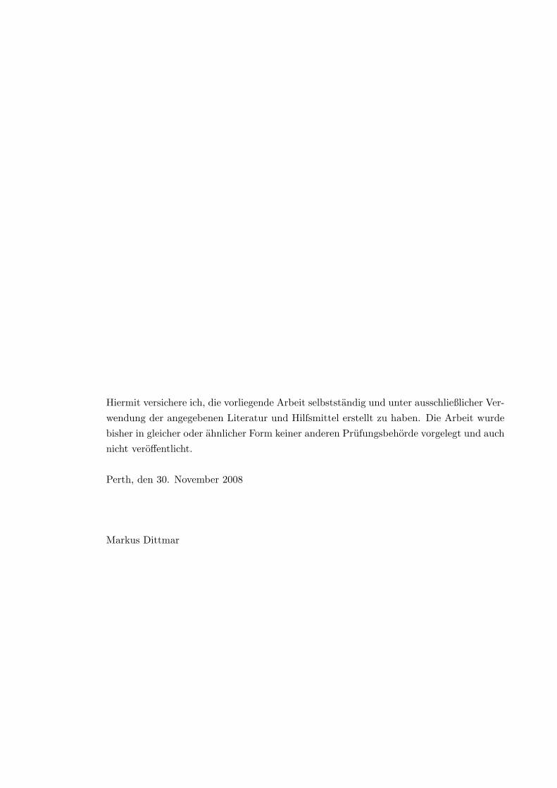
A depth sensor system, using the SenSym SX15GD2 pressure sensor, was introduced byElliot Alfirevich in 2005 for on-board usage [22] to measure the absolute depth of Mako. Itwas reported with an operating range of 0 to 5m. It outputs an analogue value from 0 to5V which is digitised by one of Mako’s A/D-converter, thus using the full accuracy of 10bits. The application note assures sufficient characteristics for its arranged operations [21].Typical values are:

• 0.1% hysteresis of its full scale range

• sensitivity of 0.1mV

• response time of 0.1ms

At the beginning of this thesis, the system was completely destroyed due to a faultyseal and had to be replaced and recalibrated.

3.4 Sensors in SubSim

The physical model of Mako in SubSim is realized by a simple box with the dimensionsx ∗ y ∗ z, a PAL Body Box [25]. PAL itself supports connected bodies to allow differentshapes presented by multiple bodies. This was not implemented in SubSim and has aninfluence to the physics as it can be seen in chapter 5.

31

Chapter 3. Sensors

Figure 3.4: a) depth sensor system schematics [22], b) typical noise of the appliedSenSym SX15GD2 pressure sensor [21]

PAL sensors have to be always attached to a parent body like a PAL Body Box.Their initial position and orientation are set in a relative term to their parent’s body ifappropriate. This is done with 3D vectors, one vector indicates the orientation, the otherindicates the position.

Physic engines like Newton Game Dynamics allows to choose custom defined units.For SubSim the basic units are “meter” for length and distances, “seconds” for the time,“radians” for angles, “kg” for weight and “Newton” for forces are used. Respectivelyis the output of the PAL sensors defined with these units, which are accessible throughthe low-level API. However in SubSim access to the sensors is also possible on a highlevel through the emulated EyeBot controller plugin, and thus different output units arepossible. Adding new sensor classes to the application and attaching them on a submarinemodel makes it necessary to update the HDT respectively.

PSD sensor : a positional sensitive device measures the distance from its body to thenearest surface which blocks the line of sight. In SubSim a single ray is projectedfrom the sensors position into the sensors direction until it reaches an object, thusdetermining the intersection point. The return value is the length of this ray. Thehigh-level distance is returned in millimetres.

Inclinometer : an inclinometer returns the angle which depends on the orientation ofits body. The return value is the angular difference of its current and the initialorientation. The body of inclinometers are always attached to the dead centre ofits parent’s body, thus an orientation vector is not present. The orientation vectorindicates the initial orientation which indicates implicitly the reference plane.

Gyroscope : this class of sensor is very similar to the inclinometer class. The returnvalue is the angular velocity, calculated with the comparison of angular orientationsin constant time intervals. A sensor instance needs also one vector to indicate its

32

3.4. Sensors in SubSim

reference plane and is attached to the dead centre of its parent’s body.

Compass : a SubSim compass sensor is identical to an inclinometer with its referenceplane along the x- and z-axis. It is located at the dead centre of its parent’s bodyand the high-level return value is between 0 and 359 degrees.

Velocity sensor : the return value of this sensor in version 2.3 was the absolute velocityof it’s attached body. Within this thesis the possibility to influence objects with asteady flow was implemented inside the simulation. Thus the sensor was adjustedto return the velocity relative to the water.

Sonar : in version 2.3 of SubSim a sonar was not available. Since sonar sensors are avery common sensor class for submarines and one of Mako’s most important sensorsystem, the implementation of a sonar sensor class was an important part of thisthesis. To simulate sonar systems is a big challenge in itself. Due to the factthat Mako’s operation environments are of simple shapes like rectangles or ovals(appendix A), a simplified sensor was implemented. This sensor class inherits thefunctionality of the PAL PSD sensor class and extends it with additional attributes.

Depth sensor : a depth sensor class was implemented within this thesis and gives theopportunity to measure the absolute distance to the virtual water surface.

Camera : camera instances simulate a robots camera to receive images from the robotsenvironment. The camera class extends the functionality of the synthetic camera,which is used to visualize the environment on the applications canvas. Two vectorsindicate their position and orientation relative to the attached body.

33

Chapter 3. Sensors

Figure 3.5: Inheritance class diagram of the SubSim sensors. One device class is imple-mented with up to 6 level of inheritance

34

Chapter 4

System Identification Mako

After studying the characteristics of sensors, several static and dynamics experimentswith Mako and it’s sensor suite were processed. These experiments have been necessaryto identify Mako under operational conditions. The outcomes of the experiments werenot only beneficial for the model adaption of SubSim, weaknesses and short comings couldbe highlighted, test procedures will be discussed and the results can be used for futureprojects.

4.1 Depth Sensor

Elliot Alfirevich conducted experiments with the depth sensor as part of his final yearproject [22]. His methods and results have been found sufficient for the purposes of thisthesis.

The first experiment was processed to indicate the influence of electromagnetic inter-ference (EMI) and supply voltage noise produced by the pulse width modulation from themotor drives. Fast on and off switching of the motors leads to a sudden increase of theelectric current on the power supply. Since depth sensor and motors are connected to thesame power supply, this has a strong effect on the accuracy of the depth sensor. Figure4.1 shows the effect of different PWM settings of the stern motor. The stern motor isthe closest to the depth sensor, thus the strongest EMI effects have been observed usingthis motor. A simple low-pass filter however could reduce the effect of both noise sourcessignificantly.

The results of the second experiment (figure 4.1) demonstrates the output linearity ofthe sensor. As shown in chapter chapter 3 the sensor shows a good linearity. At eachmeasurement depth four sensor readings were taken.

4.2 Compass

The digital compass has been found to be the most reliable sensor analyzed within thisthesis. The accuracy of 2 ◦ given in the data sheet could not be verified. It indicates

35

Chapter 4. System Identification Mako

Figure 4.1: Influence of the PWM of the stern motor on the depth sensor [22]

Figure 4.2: Actual depth against depth sensor reading [22]

36

4.3. Motors

the precision of this sensor rather than its accuracy. A reason might be that the sensoris very close attached on the aluminium tray what influences the sensors environment.Furthermore, this sensor has shown a strong reaction to tilts. Compass errors due tiltmeasurements can be quite significant [41] and depending on the geographical locationand inclination of the compass measurements can lead to different results.

To examine the effect of a tilt of 5 ◦ an accurate experiment was designed and executed.A tilt of 5 ◦ represents an usual operational condition of Mako, since it is influenced bywind and waves when it is not submerged. When Mako accelerates it experiences a jigglingbehaviour as will be shown within this chapter. Under submerged conditions a slope mightoccur due to non-uniform thrusts of the stern and bow motor.

Before the experiment the compass had to be recalibrated due to a high output non-linearity. The RoBIOS provides the function COMPASSCalibrate(int mode) to calibratethe sensor. This function has to be called twice. The second call has be done after thesensor is turned around 180 ◦.

The hole tray of Mako’s upper hull was clamped in an adjustable bench vise to set upa tilt of 5 ◦. The bench vise itself was mounted on a turn table, thus it was possible toturn the tray about 360 ◦ precise around the perpendicular axis.

Figure 4.3: Absolute heading error of the digital compass with a tilt of 5 ◦ and without

4.3 Motors

During experimentation it could be observed that Mako tends to turn right when settingthe same thrust on port and starboard actuator. Gonzales [22] processed thrust measure-ments with a load cell on all actuators. All four motors produced different thrusts whensetting them to the same PWM. Gonzaless solution was to implement a look-up table inthe motor controller to balance the different forces on the actuators. Thus it was possibleto set each motor to a similar thrust with ease.

Since the motors are inexpensive trolling motors and especially with the horizontal

37


motors being used by many experiments from 2004, a considerable amount of wear wasassumed. Due to the fact the motors are fixed to Mako’s body thrust tests with a load cellcould not be repeated. Instead an optical tachometer was used to measure the revolutionsof the propellers. Each propeller consists of three propeller blades, so that the results ofthe tachometer had to be divided by three.

The tachometer provided its output on a LCD display. The output was updated 1.5times per second. To capture the readings contiguous, movies of the display were recordedwhich could be played in slow motion afterwards. The readings were processed with a stepsize of 3% of the maximum pulse width beginning with 0% (full speed due to the invertedlogic) until the motor stopped. For each motor and each pulse width modulation, 30contiguous readings were captured and the arithmetic average was calculated. The resultsof the bow motor are shown in figure 4.4 and 4.5 in relation to the thrust measurementsfrom 2004. A linear dependency between revolution per minutes (RPM) and producedthrust can be seen. However, the experiment shows that the motors still rotate with higherpulse width modulation than in the experiments done in 2004. One reason is the missingwater resistance since the revolution experiment was processed with the actuators in air.Another reason because of wear the motors are run in and experience a lower resistance.

Figure 4.4: Motor revolution versus actuator thrust force, bow motor forward direction

As a result the look-up table was respectively updated. The results of the other motorscan be found in appendix C.

Figure 4.6 also indicates how the speed of the motors fluctuates. The motors are onlycontrolled by the PWM without any feedback to control the actual speed. Higher speedshave a higher fluctuation.

38

4.3. Motors

Figure 4.5: Motor revolution versus actuator thrust force, bow motor reverse direction.A much lover thrust can be observed due to motor and propeller optimizations to operatein forward direction

Figure 4.6: Fluctuation of the bow motor in forward direction

39


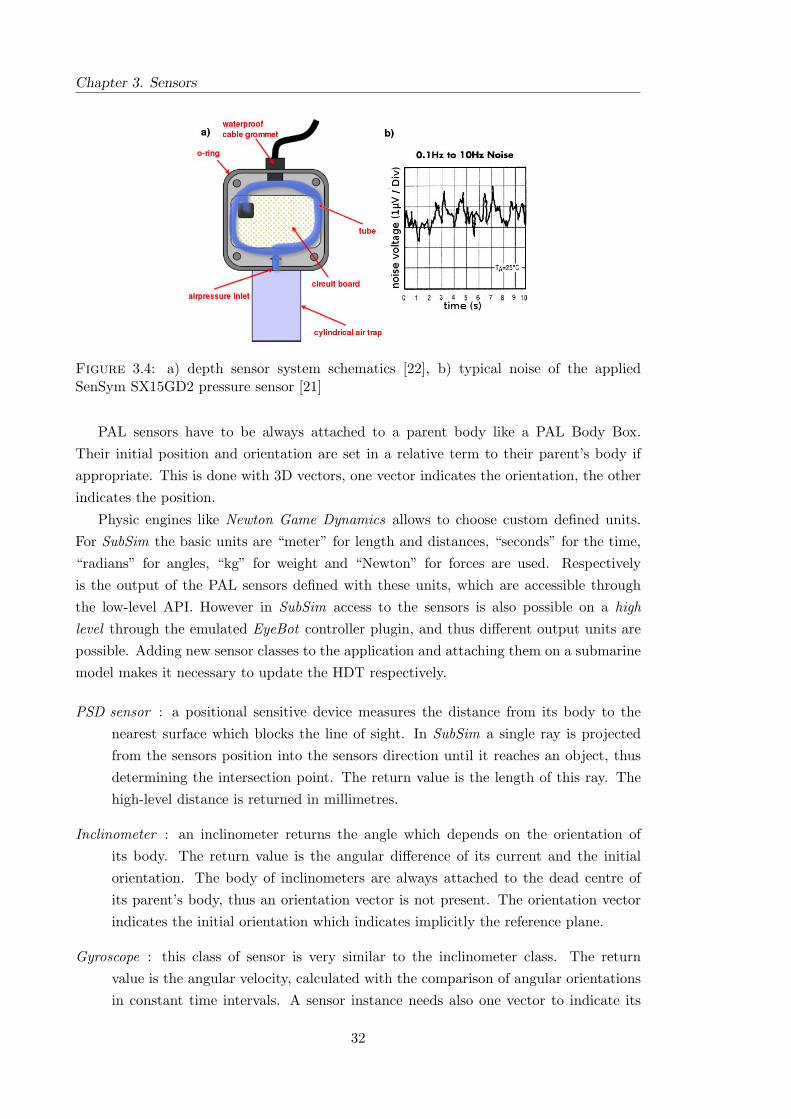
4.4 Sonar

The sonar system works well only in a water environment, and large space is necessaryto avoid disturbing reverberations. This makes it necessary to process experiments withthe sonar in a environment such as a pool. The shortcomings mentioned by Nguyen inhis final thesis were replicated within this thesis [50]. Many experiments by Nguyen andAlfirevich were processed to analyze the sonar system and especially the sonar transducerwithout the sonar controller. Since the the transducers are fixed mounted on Mako, and noseperate transducer has been available, these experiments could not repeated within thisthesis. However, more roughly static and dynamic experiments were processed with thewhole Mako involved, and the behaviour could be verified which was observed by previousexperiments. For transducer experiments both Alfirevich and Nguyen, used a digitallyoutput from the EyeBot microcontroller to create the input signal for the transducer. Thereturning signal was again received by the microcontroller, thus replacing the function ofthe sonar controller to retrieve transparent results from the transducer. This was quitehelpful since the sonar controller provides data with a rate of only 1Hz. One measureddistance value from the controller is obtained from multiple samples which the controllergenerates.

The results shown in figure 4.7 show the detection rate of samples in a static situation.Individual signals were sent out orthogonal to a wall and reflected on its surface. Therequired detection rate was defined with a minimum of 50% to be sufficient for navigatingpurposes.

Figure 4.7: Static detection rate for different distances [50]

As experienced within this thesis, the detection rate decreases with a deviation fromthe surface normal until the transducer leaves the beam width of the signal (Figure 3.2b).

Figure 4.8 shows the result of a dynamic experiment. The transducer was directed toa wooden rod. This rod was moved then several times perpendicular to the transducer ina distance from 0.5 meters to 2 meters. The effect shows in a lower detection rate. Onereason for this is the produced distortion of the water which comes along with environ-

40

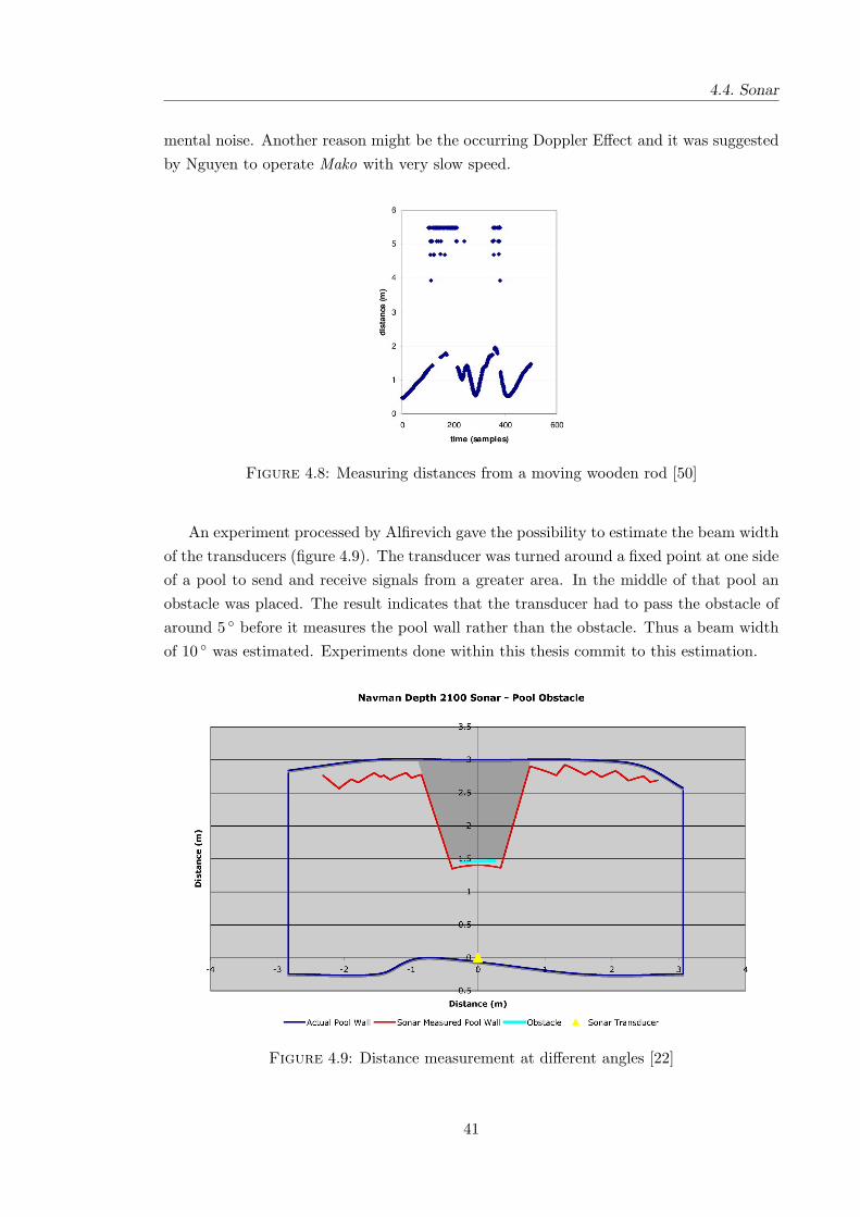
4.4. Sonar

mental noise. Another reason might be the occurring Doppler Effect and it was suggestedby Nguyen to operate Mako with very slow speed.

Figure 4.8: Measuring distances from a moving wooden rod [50]

An experiment processed by Alfirevich gave the possibility to estimate the beam widthof the transducers (figure 4.9). The transducer was turned around a fixed point at one sideof a pool to send and receive signals from a greater area. In the middle of that pool anobstacle was placed. The result indicates that the transducer had to pass the obstacle ofaround 5 ◦ before it measures the pool wall rather than the obstacle. Thus a beam widthof 10 ◦ was estimated. Experiments done within this thesis commit to this estimation.

Figure 4.9: Distance measurement at different angles [22]

41


4.5 Velocity Measurement

To compare the surge behaviour of Mako with the model in SubSim a couple of experimentswere processed to obtain Mako’s maximum velocity and acceleration. In these experimentsa heading control using the digital compass was applied to have Mako travelling straightas possible. A control was necessary due to the fact that setting the same thrust on portand starboard motor, even with the updated look-up table, does not mean that Mako willtravel in a straight line. With the heading control Mako is able to drive almost on an idealstraight line.

All experiments were processed without submerging thus Mako travels like a ship.Because of time constraints and a destroyed depth sensor at the beginning of this thesis,not all targeted experiments could be completed. A picture in appendix E shows that,even when Mako is in a non submerged state, it is almost completely underwater and thusonly small differences to submerged experiments are expected.

Figure 4.10: Maximum velocity of Mako at 100% thrust

Since the accelerometer does not provide a sufficient sensitivity, and the velocity sensorhas a low resolution, a different method had to be found to obtain the wanted data. Awater tight camera was mounted on top of the camera facing to the port side of thesubmarine. At the inside of a pool wall a 10 meter long measuring tape with large scalemarkings was attached. Movie records with a resolution of 30 frames per second weretaken from this measure tape. This gave the possibility to step through movie afterwardsframe by frame to measure the progress of Mako in forward direction in respect to thetime.

The maximum velocity of Mako was determined by setting both horizontal motors to100% thrust. For the acceleration experiment Mako was accelerated from a stationaryposition and suddenly accelerated by setting port and starboard motor to 100% thrust.The deceleration data were gained by switching off both motors while running Mako atfull speed.

42

4.5. Velocity Measurement

Through the recorded movies the progress in respect to the measure tape was deter-mined each 200 milliseconds. The result is shown in the figures 4.10, 4.11 and 4.12. Anaverage maximum velocity of 5 ∗ 8.8cm

200ms = 44cm/s has been determined. The fluctuationof the values shown in figure 4.10 can be explained by the jiggling Mako experiences inport/starboard direction while driving straight. Mako reaches its maximum velocity after6 seconds and returns after 32 seconds of drifting from the full velocity to a stationaryposition. Figure 4.11 shows also the result of the velocity sensor. The sensors output wasdivided by 5 to adjust it to the determined velocity with the camera. The outputs gradualrise is an indication of the low resolution of the sensor. With higher velocities the sensorsaccuracy decreases.

Figure 4.11: Determined velocity at full acceleration from a stationary position

Figure 4.12: Drifting from maximum velocity to a stationary position

43


4.6 Acceleration

The velocity measurements also allowed the determination of Mako’s maximum and mini-mum acceleration. Reading the maximum progress from figure 4.11 implicates the highestacceleration is 9.5cm/s2 ≡ 9.7mg. Due to the jiggling behaviour of Mako this value canbe regarded as an upper bound. The data obtained during this experiment from the ac-celerometer did not indicate any detectable acceleration. This is because of a too lowsensitivity of the sensor. The sensitivity in the data sheet [18] is given with 800mV/g.The maximum detectable difference in the output voltage is thus

∆Vmax = resolution ∗ acceleration (4.1)

∆Vmax = 800mV

g∗ 0.0097g (4.2)

∆Vmax = 7.76mV (4.3)

The A/D converter of the EyeBot microcontroller has a resolution of 5V/10bit =4.883mV . Assumed the A/D converter has an offset of 0.5LSB (least significant bit) themaximal detectable digital difference will be 1.58LSB, since

7.76mV − 1.5 ∗ 4.883mV = 0.44mV < 4.883mV/2 (4.4)

Considering that the sensors typical noise influence is given as 4.7mV rms [18] it be-comes obvious that almost no acceleration of Mako is detectable by this sensor. Thismeans the sensor unusable for navigation purposes.

The method to gain the maximum acceleration values for the sensor applied by deGauchy [34], by simply shaking the sensor with the hands in different directions, doesnot lead to reasonable results. The results were not repeatable since the applied force isunknown.

To calibrate the sensor it’s axis of sensitivity has to be turned into the direction ofgravity to gain the acceleration of 1g and reversed to gain the acceleration of −1g where gis the acceleration of gravity. The output function of the sensor follows the sinusoid, thushaving the highest sensitivity at 0g and the lowest at ±1g.

Figure 4.13 shows the calculated output line of the sensor at V dd = 2.6V . To verifythe sensors sensitivity it was turned ±90 ◦, ±45 ◦ and 0 ◦ to the surface normal for eachaxis and 50 samples from the output of the A/D converter in each position were recorded.The results of the y- and z-axis can be found in appendix D.

4.7 Spot Turn

An experiment was processed to determine how fast Mako can turn 360 ◦ around the yawdirection. Therefore either port motor was set to 100% forward thrust and the starboard

44

4.7. Spot Turn

Figure 4.13: Angular response of the accelerometer

Axis -90 ◦(LSB) -45 ◦(LSB) +0 ◦(LSB) +45 ◦(LSB) +90 ◦(LSB)

x 1.31 1.5 1.34 1.24 1.2y 1.2 1.32 1.31 1.26 1.14z 1.17 1.19 1.25 1.07 1.08

Table 4.1: Measured standard deviation of the accelerometer over 50 samples

motor to 100% backward thrust or vice versa. This did not lead to a spot turn due tothe fact Mako traveled in a circle as shown in figure 4.14. Forward and backward thrustof the motors are quite different as it can be seen in figure 4.4 and 4.5. To determine theway Mako traveled a movie of the scene was recorded. Therefore a camera was mountedon a 4.5m high stand directly over Mako. For an anti-clockwise turn Mako needed 23.17seconds, for a clockwise turn 23.5 seconds were measured. A picture of the experimentsetup can be found in appendix E.

Figure 4.14: Travel way of Mako in anti-clockwise direction with 100%thrust forwarddirection on the starboard motor and backward direction on the port motor

45


4.8 Wall Following

The wall following problem is the first competition task from the project Mako initiative.It has been used to evaluate the sonar system with FUZZY and PID controllers by Alfire-vich, Daws and de Gauchy during their final year projects. However the results of theirexperiments were not always repeatable and therefore not reliable as already mentionedby Daws [33]. The problem is the shortcoming of the sonar system. The data rate is tooslow, the output data has a too high resolution, and with a moving Mako a certain degreeof rejection rate is unavoidable. An additional problem occurs when Mako tries to correctthe distance and thus changing the angle of the sensor in respect to the wall. The greaterthe angle between the transducer normal and the the normal from the wall the greater isthe measured distance from the sonar as seen in figure 4.15a). The feedback of the sonarused as input value for the FUZZY or PID controller lead to a even stronger correction.

Figure 4.15: a) The turning transducer problem, b) the new transducer setup

A new transducer setup was chosen to reduce this effect and to increase the effectivebeam width of the transducer. Two transducer on the port side and two on the bow weremounted, each with an offset of 15 ◦ of their respective axis. The setup can be seen infigure 4.15b). Additionally to avoid Mako turning out of the beam width, the controlprogram applied for this task used the information from the digital compass to narrow thepossible turn angle. Crosstalking is avoided with the help of the multiplexer. Only onetransducer from a pair of two transducer at each side is active at the same time.

Since it is unknown from which transducer the returned value from the multiplexeris three readings were taken to ensure readings from two different transducers. The firstreading from the transducer 1, the second from transducer 2 and the third again fromtransducer 1 for each pair. The shortest distance of all three received values was takenas the controller input. This however lead to a significant time overhead. The total timefor three readings was determined with 4.8 seconds in average and forced a very slowoperation speed for Mako.

Regardless the new setup has proven more robust and with the help of the digital com-pass Mako passed for the first time a rectangular corner autonomously thus accomplishing

46

4.8. Wall Following

the first mission task of the project Mako initiative.The result of a FUZZY wall following experiment is shown in figure 4.16. Mako tried

to keep a distance of 10dm of its port side. The average thrust on port and starboardmotor was set to 10%. The effective distance is the smallest distance determined by thetwo transducers on the port side. Velocity measurements with the velocity sensor did notlead to reasonable results due to the low resolution of the sensor and the low operatingvelocity applied at this experiment. A successful run with a PID controller could not beaccomplished due to time constraints.

Figure 4.16: The result of a FUZZY wall following experiment

47

Chapter 5

Simulation Model Adaption

The experiments done in chapter 4 were necessary for the model adaption to fill thereality gap in SubSim. With the observations and results of the experiments a detailederror model could be implemented within this thesis. SubSim reached its version status2.4. To evaluate the changes on SubSim the same experiments designed and processed forMako were repeated in SubSim, using the same control programs. However, the RoBIOSAPI does not provide access to all sensors attached on Mako. E.g the RoBIOS does notsupport velocity sensors and deals not with a multiplexer system used for the sonar. TheEyeBot plugin in SubSim was emulated to represent its original counter part, including theRoBIOS API. The decision was made to write a wrapper API, which allows to run controlprograms written for Mako, without any changes in SubSim. This enables applications tobe written for Mako without considering the implementation of the API in SubSim. Notchanging the EyeBot plugin specifically for Mako also ensures a consistent and independentinterface for different robots using the simulation.

5.1 Drag, Buoyancy and Propulsion in SubSim

In SubSim the physics engine is responsible for calculations of the physical model. Aliquid model provided by a physics engine to simulate water has not been implemented.Therefore a fake buoyancy and drag was implemented to simulate the liquid effects ofwater.

In SubSim version 2.3 the body of Mako was represented by a PAL box with thedimensions 1.8m∗0.5m∗0.5m which results in a volume of 0.45m3. The weight of the bodywas given with 500g and the density of the liquid with ρ = 0.99829kg/m3. These settingscoupled with an error in the buoyancy calculation lead to a physical model, which allowsthe Mako model to travel in its environment under ideal conditions with no noticeableeffects of draft and drift. Tasks like “wall following” can be accomplished with ease, thusmaking sophisticated controls unnecessary.

49

Chapter 5. Simulation Model Adaption

The applied formula in SubSim for the liquid drag is:

D =12∗ ρ ∗ Cd ∗A ∗ v2 (5.1)

Where D is the applied drag force in Newton (N) on the object body like Mako, ρ isthe fluid density in kg/m3, A is the frontal surface of the object in m2(PAL Box) and v

the relative velocity in m/s2 [25]. The fake buoyancy is calculated by dividing the modelsvolume in four equal spheres, calculating their buoyancy and applying impulses on fourdifferent symmetrical points on the body. This enables an even appliance of impulses tostabilize the body (figure 5.1).

Figure 5.1: The fake buoyancy Model of SubSim

Changing the density of the fluid to ρ = 998.29kg/m3 and the weight of the Mako thatit produces a buoyancy similar to the real Mako lead to a series of reactions, since it hasalso a major influence on the propulsion and drift model. Due to the fact that no unitswere specified anywhere the impact of this outcome could not be foreseen at the beginningof this thesis.

The propulsion model is implemented by propeller by class, which simulates a propelleractuator and a corresponding DC motor. The simplified formula to calculate the appliedthrust on an attached body is

T = αlumped ∗ V (t) (5.2)

where αlumped is an experimentally determined lumped parameter and V the voltagewhich is set by a control program. No units for this formula are specified.

Another outcome was found via running experiments on SubSim with different simu-lation speeds. Different speeds lead to different results. The problem is a lack in synchro-nisation with the simulation time and real time, but it does not effect the physics itself asseen in figure 5.2. Despite the fact that with different simulation speeds the model travelsthe same path, the model travels different speeds. For a simulation speed of “5”, the Makomodel needs 38.5 seconds of simulation time to complete one circle. With a speed of “15”it needs 40 seconds and with a speed of “30” it needs around 70 seconds. The modeltravels an ideal circle with a diameter of around 1.3 meter. The real Mako needs only 0.8meter.

50

5.1. Drag, Buoyancy and Propulsion in SubSim

Figure 5.2: Anti-clockwise Spot Turn Experiment, with three different simulation speedsand changed physical model

Figure 5.3 and 5.4 show the results of acceleration experiments in SubSim using thesame heading control as being used for Mako. Three different simulation speeds show theeffect of the lack of synchronisation. Figure 5.4 shows that the model travels differentdistances within the same time. The maximum velocity of this model was determined tobe 9cm/s in comparison to 44cm/s for its real counterpart. This is explainable due to theinexistence of an appropriate physical model.

Figure 5.3: Velocity of the Mako model during the acceleration in SubSim with differentsimulation speeds and changed physical model

Due to the fact that the physical object of Mako model does not contain informationabout applied forces or accelerations on its body, no accelerometer could be implementedinto Makos sensor suite in SubSim.

51


Figure 5.4: Surge progress of the Mako model in SubSim during the acceleration with100% thrust, different simulation speeds and changed physical model. Significant differenttravel distances can be seen at different simulation speeds

Figure 5.5: Surge progress of the Mako model in SubSim during the deceleration from100% thrust, different simulation speeds and changed physical model

In theory it is possible to determine acceleration of a body with:

a =∆v∆t

(5.3)

Where a is the acceleration in m/s2, ∆v is the difference of velocity in m/s and ∆t isthe difference in time in s. Due to a non consistent simulation time in SubSim, applyingthis formula does not lead to reasonable results.

5.2 Error Model

As the experiments in chapter 4 have shown, introducing a noise model to SubSim is crucialto test, improve and evaluate the robustness and reliability of control algorithms writtenfor Mako. EyeSim played a role model for developing and implementing a noise model forSubSim. However the noise model in EyeSim is based on a statistical noise model. Theresults and the experience gained within this thesis resulted in an implementation of anerror model not only based on a statistical model.

Before noise classes were defined and implemented, it was necessary to determine theoutput units for each single sensor class. As already described in chapter 2, the basic unitsmeter for distances, rad for angles and seconds for time are used for the return values ofthe sensors.

52

5.2. Error Model

As in EyeSim all sensors and the actuators can be influenced with a standard normaldistribution with zero mean. Depending on the output value for a certain sensor class thevariance of the distribution can be changed. The central limit theorem method was chosento produce the standard distribution [55]. An appropriate algorithm was found at [35].The model implemented in SubSim can be described by

f [i] = s[i] + n[i] (5.4)

where f [i] is the resulting signal at the time i, s the unchanged source signal and n isthe standard normal distribution [45]. Further a uniform discrete distribution model wasimplemented as it was applied in [48]. It can be described by

f [i] = s[i] + u[i] (5.5)

where u is the uniform noise.

A number of different noise sources were added to each sensor class and differentsettings can be chosen. E.g the the maximum range for PSD or the sonar sensors can beadjusted. Additionally for sonar sensors, settings for the maximum angle of incidence, theresolution and the response time are available. Compass sensors can be influenced by tiltnoise and for velocity sensors the resolution can be changed. Despite the fact that thevision system is not part of this thesis, the error model for the EyeBot camera of EyeSimwas adopted. This error model consists of Salt and Pepper noise, Hundreds and Thousandsnoise and a standard normal distribution noise (Gaussian distribution) (figure 5.6). Saltand Pepper noise adds random black and white pixels to the camera image. Hundredsand Thousands noise produces colored random pixel. The standard normal deviation isapplied on all RGB (red, green, blue) channels for each individual pixel.

Figure 5.6: EyeBot plugin with activated camera: a) original image, b) Salt and Peppernoise, c) Hundreds and Thousands noise, d) Gaussian noise

53


Salt and Pepper and Hundreds and Thousands noise can be described by [45]

f(i) = (1− e) ∗ s(i) + en(i) where (5.6)

e =

{1, with probabilityPe0, otherwise

Figure 5.7 shows the designed and implemented software package “noise source‘” withavailable noise sources. A software package is a group of related classes. All noise sourcesextend the class Noise which provides a pure virtual function to apply “noise” on an giveninput value. This allows the application to register noise sources for each sensor class.Available noise sources for a sensor are kept in a list of the class SubSimNoiseDevice,which itsself extends all sensor classes and the simulated EyeBot camera.

Figure 5.7: Noise package: the noise source family

5.3 Error Model Control

The error model was implemented that it is accessible via the robot settings file or theGUI. By adding parameters into the robot settings file it is possible to preset a robotserror model for each single sensor. It allows for different robot description files of the samerobot, with different noise settings, to be defined. This comes quite handy if settings haveto be compared and used for multiple experiments.

An error GUI control was implemented and enables access to all sensors of a robotduring runtime. Allowing changes on the error model even when the control program ofa simulation has been started. The GUI control is implemented in a new frame which isaccessible trough the main frame menu bar (figure 5.8). It extends the wxFrame class andcontains a wxNotebook object [4]. The notebook acts like a register where new wxPanelscan be added as pages. Therefore each sensor class has its own panel hence enables aneasy overview over all available sensor classes.

For each single error source, for a specific sensor class the strength of the noise canbe changed with wxSliders. These are sliders which can be defined with a minimum and

54

5.3. Error Model Control

maximum range. Unfortunately floating point values are not supported.

On each sensor panel a pull down menu was implemented to allow a sensor to bechosen and thus adjusting the noise settings for each sensor individually. The names ofthe sensors in the pull down menu are equal to those in the robots settings file. Hence it ispossible to identify each sensor with ease. If no sensor of a given sensor class is attachedto a robot, the pull down menu for this sensor class indicates this simply with “none” inits text field.

Figure 5.8: Error model GUI control

It has been shown in EyeSim that visualizing sensor devices and sensor readings is ofgreat help for users in terms of debugging and understanding their applications. Withinthis thesis the visualization of PSD sensors and sonar sensors has been implemented.A PSD sensor is represented as a small black cube and indicates its localisation at therobots body. For the sonar sensors a frustum can be drawn, which indicates besides itslocalisation the beam width. This frustum changes its angle when the beam width ischanged in the error model respectively. A line, projected from the sonar sensor itsself,shows the perpendicular beam of the acoustic signal. Further, to have a instantaneousvisual feedback if the sonar sensor reads in its beam width, a line is drawn on intersectingsurfaces of surrounding objects. This line represents a normal vector, which is calculatedof the position where the beam of the sensor hits the surface. A blue line shows that thesensor reads within its beam width and switches over to red, when the sensor leaves thebeam width (figure 5.9).

To simulate steady flows in water, the error model provides the possibility to applyequal impulses on all objects within a simulation. Two sliders allow the setting of longitudeand latitude direction of a applied impulse, one slider determines the strength. To give theuser a visual feedback of the impulse an arrow is drawn above the scene. Its direction showsrespectively the direction of the applied impulse. The tail is implemented bi-coloured.Besides the arrows colour a blue line in the tail indicates the strength of the appliedimpulse.

55


Figure 5.9: Visualization in SubSim: a) frustum of the sonar beam width, b) the normalvector of a intersecting wall from a sonar beam, c) arrow indicator for steady flow

5.4 Wall Following - Comparison

The wall following experiment presented in chapter 4 was repeated in the simulationto evaluate the changes on the physics model and the newly implemented sonar sensor.Multiple runs with different parameters for the physics model were tried. Owing to aoversimplified physical model of Mako and a missing liquid model provided by the physicsengine it was impossible to find parameters, which lead to a behaviour of the model closeto its real counterpart.

In [26] a comparison between different physic engines has been processed. The ex-periments show significant different physical behaviours of different engines. To find anappropriate physic engine is therefore difficult for developers. Further it indicates howimportant it is to find physical models as close to reality as possible.

To evaluate the experiments it was attempted to repeat the method applied in [49]. Aquantitative measure of discrepancy of behaviours could be calculated with the Euclideandistance between the coordinates of a simulated and real travel path. Therefore, coordi-nates in commensurate time steps from the travel paths were taken. To record the travelpath in SubSim was accomplished with ease, this was not the case for the real Mako.The stand used for the sport turn experiment was not high enough. A visible distance ofonly 5.5 meter could be recorded with the applied camera, to less for a comparison. Therecorded movies however can be used for documentation purposes.

Because of this drawback the following two charts were designed to have a visible feed-back of the control data. Both diagrams show the results of a wall following experiments.The same control program as it was used by experiments on the real Mako was applied,and the same sonar setup was attached to the model as used for the experiment describedin chapter 4.

The first chart 5.10 shows five different runs of the wall following experiment withdifferent settings on the error model. Different settings in terms of the sensor resolutionand the response time were applied to visualize the effective difference. The responsetime is applied for each sensor individual. Thus multiplying this time by four gives theabsolute response time. The higher the resolution and the higher the response time is setup, the more time it takes until the model reacts to correct its distance. A setting with the

56

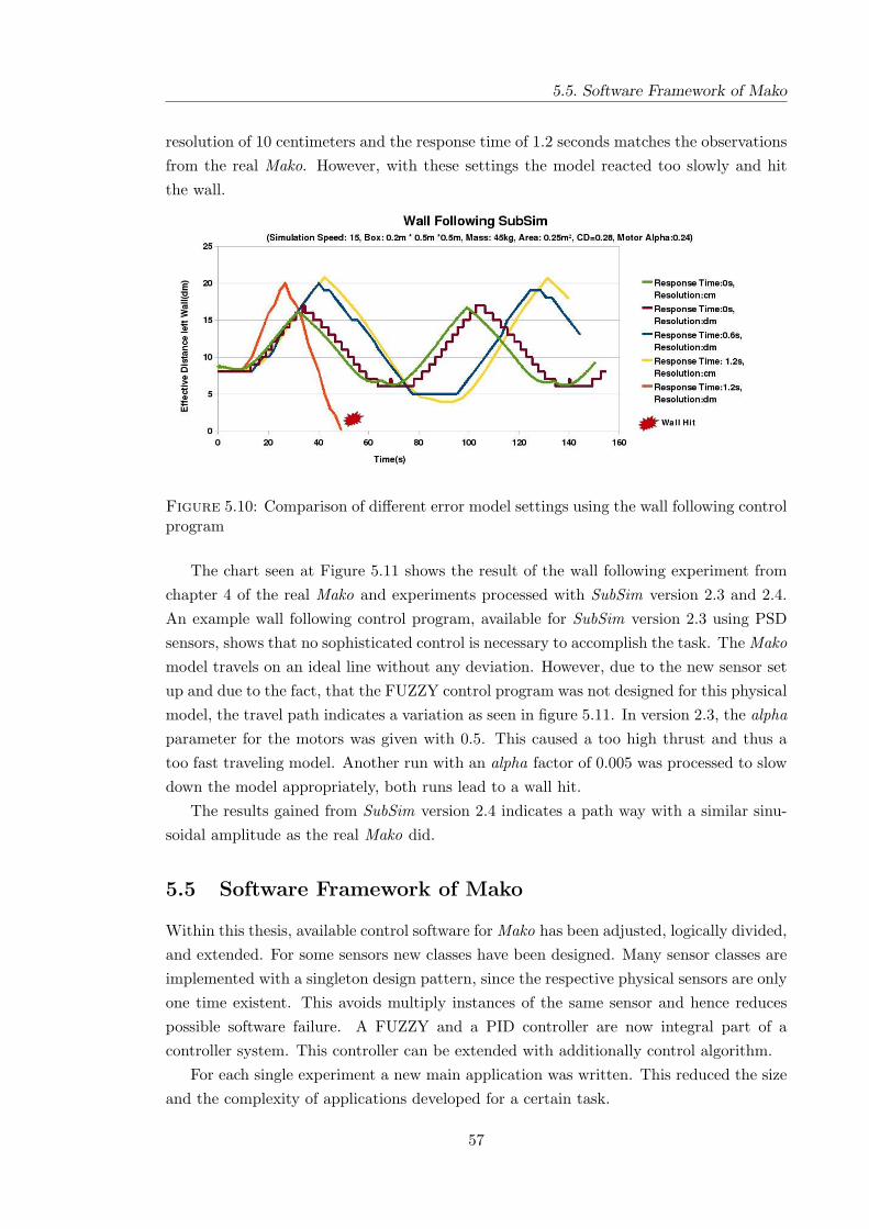
5.5. Software Framework of Mako

resolution of 10 centimeters and the response time of 1.2 seconds matches the observationsfrom the real Mako. However, with these settings the model reacted too slowly and hitthe wall.

Figure 5.10: Comparison of different error model settings using the wall following controlprogram

The chart seen at Figure 5.11 shows the result of the wall following experiment fromchapter 4 of the real Mako and experiments processed with SubSim version 2.3 and 2.4.An example wall following control program, available for SubSim version 2.3 using PSDsensors, shows that no sophisticated control is necessary to accomplish the task. The Makomodel travels on an ideal line without any deviation. However, due to the new sensor setup and due to the fact, that the FUZZY control program was not designed for this physicalmodel, the travel path indicates a variation as seen in figure 5.11. In version 2.3, the alphaparameter for the motors was given with 0.5. This caused a too high thrust and thus atoo fast traveling model. Another run with an alpha factor of 0.005 was processed to slowdown the model appropriately, both runs lead to a wall hit.

The results gained from SubSim version 2.4 indicates a path way with a similar sinu-soidal amplitude as the real Mako did.

5.5 Software Framework of Mako

Within this thesis, available control software for Mako has been adjusted, logically divided,and extended. For some sensors new classes have been designed. Many sensor classes areimplemented with a singleton design pattern, since the respective physical sensors are onlyone time existent. This avoids multiply instances of the same sensor and hence reducespossible software failure. A FUZZY and a PID controller are now integral part of acontroller system. This controller can be extended with additionally control algorithm.

For each single experiment a new main application was written. This reduced the sizeand the complexity of applications developed for a certain task.

57


Figure 5.11: Comparison of SubSim version 2.3, 2.4 and Mako using the wall followingcontrol program

Experiences from experiments have shown that it is crucial to have fully customizableapplications during runtime. This enables the setup of a control program with ease and toreact to unforeseeable conditions. Therefore, much effort was spent for the user interface.As a result a full software framework Mako could be implemented and is available forfuture projects. A class diagram is shown in figure 5.12.

Figure 5.12: Software Framework of Mako

58

Chapter 6

Conclusions and Future Work

The comparison between SubSim version 2.3 in chapter 5 has indicated how big the realitygap has been at the begin of this thesis. Due to the implementation of the error modeland the changes of the physical model a much closer behaviour to the real counterpartwas accomplished. For the first time a controller program written for Mako was appliedsuccessfully in SubSim. The API wrapper and the new added sensor classes for SubSimallows now testing control programs in a simulated environment before testing it on thereal Mako. This means a major improvement for software developing and debugging.The implementation of a steady force allows now more realistic simulations for offshoreenvironments. SubSim reached version status 2.4 successfully.

A new sonar setup for Mako was applied and has proven more robust for the wallfollowing task. The depth sensor system was replaced, calibrated and its water tightnesswas assured. It will be available for future projects. For the first time the first missiontask of the project Mako initiative was accomplished by passing successfully a rectangularcorner.

6.1 Mako

Makos body has proven robust, stable and well balanced. The solution of mounting allinertial devices on a tray inside the upper hull enabled easy access. Thus smaller defectscould be repaired while conducting experiments. The maximum velocity speed has beenfound more than sufficient, since speed is not a matter of the missions tasks.

The velocity sensors resolution is too low to gain reasonable output values. The ac-celerometer is not applicable for navigational purposes due to its too low sensitivity. Astable communication with the sonar multiplexer could be accomplished after fixing aproblem with floating input gates. With only 4 transducers it is impossible to navigateMako through an unknown environment, even with very low velocity. Due to the fact thatthe vision system is not in service no image processing can be applied.

The platform Mako posses the prerequisites to accomplish its mission task but suffersunder its insufficient sensor suite.

59

Chapter 6. Conclusions and Future Work

6.2 SubSim

An additional plugin might be introduced which simulates the needs of Mako and replacingthe developed wrapper API used within this thesis, thus having multiple micro controlleremulators for SubSim.

The simulation posses an easy to use GUI interface. The possibility to preset the envi-ronment via many settings files makes the application highly customizable. The XML fileformat ensures readability for users. Many available examples are assistant for developingnew environments, robots and control programs.

The implementation of a multiple layer architecture keeps the software developmentclear. However the lack of documentation will be drawback for new developers. The waythe physics engine is implemented might confuse developers. The possibility to updatePAL with ease is not given. Specific changes for SubSim were applied. These changes arenecessary to provide the functionality needed by SubSim.

For the future it is recommended to improve the physical model and to provide adeveloper documentation. Introducing new features to SubSim, without re-factoring itscurrent state, will increase complexity, thus becoming a bottle neck.

60

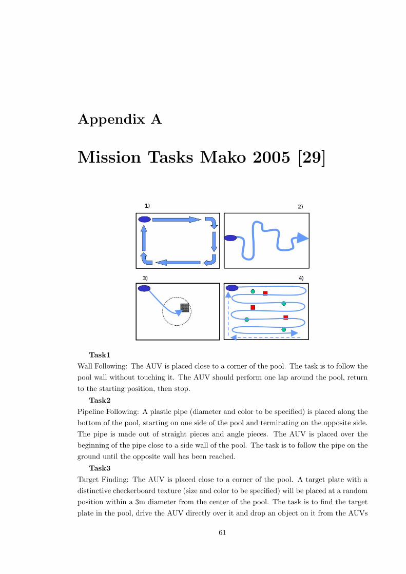
Appendix A

Mission Tasks Mako 2005 [29]

Task1

Wall Following: The AUV is placed close to a corner of the pool. The task is to follow thepool wall without touching it. The AUV should perform one lap around the pool, returnto the starting position, then stop.

Task2

Pipeline Following: A plastic pipe (diameter and color to be specified) is placed along thebottom of the pool, starting on one side of the pool and terminating on the opposite side.The pipe is made out of straight pieces and angle pieces. The AUV is placed over thebeginning of the pipe close to a side wall of the pool. The task is to follow the pipe on theground until the opposite wall has been reached.

Task3

Target Finding: The AUV is placed close to a corner of the pool. A target plate with adistinctive checkerboard texture (size and color to be specified) will be placed at a randomposition within a 3m diameter from the center of the pool. The task is to find the targetplate in the pool, drive the AUV directly over it and drop an object on it from the AUVs

61

Appendix A. Mission Tasks Mako 2005 [29]

payload container. (AUVs without the ability to drop a payload should just hover overthe target plate).

Task4

Object Mapping. A number of simple objects (balls and boxes, color and sizes to bespecified) will be placed near the bottom of the pool, distributed over the whole pool area.The AUV starts in a corner of the pool. The task is to survey the whole pool area, e.g.using a sweeping pattern, and record all objects found at the bottom of the pool. TheAUV shall return to its start corner and stop there. In a subsequent data upload (AUVmay be taken out of the pool and a cable attached to its on-board system), a map of someformat should be uploaded that shows location and type (ball or box) of all objects foundby the AUV

62

Appendix B

Class Diagrams

B.1 Full class diagram SubSim version 2.4

Figure B.1: Full class diagram of SubSim version 2.4

63

Appendix B. Class Diagrams

B.2 Class Diagram SubSimDevices

Figure B.2: Class diagram software package SubSimDevices of SubSim version 2.4 withmembers

64

Appendix C

Motor Characteristics

Figure C.1: Motor revolution versus actuator thrust force, stern motor forward direction

Figure C.2: Motor revolution versus actuator thrust force, stern motor reverse direction

65

Appendix C. Motor Characteristics

Figure C.3: Motor revolution versus actuator thrust force, port motor forward direction

Figure C.4: Motor revolution versus actuator thrust force, port motor reverse direction

66

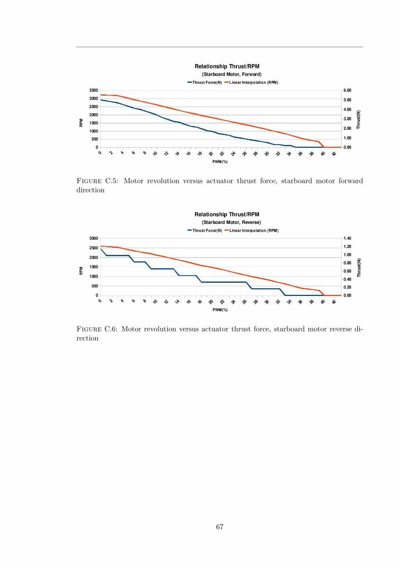
Figure C.5: Motor revolution versus actuator thrust force, starboard motor forwarddirection

Figure C.6: Motor revolution versus actuator thrust force, starboard motor reverse di-rection

67

Appendix D

Accelerometer Characteristics

Figure D.1: Angular response of the accelerometer y-axis

Figure D.2: Angular response of the accelerometer z-axis

69

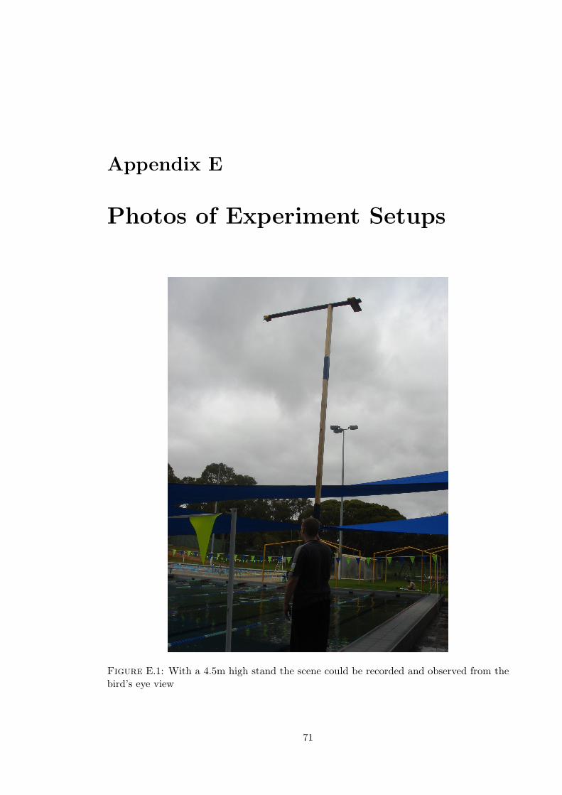
Appendix E

Photos of Experiment Setups

Figure E.1: With a 4.5m high stand the scene could be recorded and observed from thebird’s eye view

71

Appendix E. Photos of Experiment Setups

Figure E.2: A 10m long measure tape was attached on the wall to determine the velocityof Mako

Figure E.3: An optical tachometer was used to measure the revolutions of the propellers

72

Appendix F

Upper and lower PVC Hull

Figure F.1: The upper PVC Hull and the Tray with internal sensors, the sonar multi-plexer and EyeBot microcontroller

Figure F.2: The lower PVC Hull with its containing three batteries for the power supply

73

Appendix G

Multiplexer Circuit Diagram

Figure G.1: The multiplexer of the sonar system. The red circle highlights the opengates [33]

75

References

[1] Underwater robots. [online], 2008. Available: http://ezinearticles.com/

?Underwater-Robots&id=408074.

[2] Newton game dynamics. [online], 2008. Available: http://www.newtondynamics.

com/.

[3] Physx by nvidia. [online], 2008. Available: http://www.nvidia.com/object/

nvidia_physx.html.

[4] wxwidgets - cross platfrom library. [online], 2008. Available: www.wxwidgets.org.

[5] Tinyxml. [online], 2008. Available: http://www.grinninglizard.com/tinyxml/.

[6] Hydroid, inc. [online], 2008. Available: http://www.hydroidinc.com/contact.

html.

[7] Kongsberg maritime. [online], 2008. Available: http://www.km.kongsberg.com/.

[8] Bluefin robotics. [online], 2008. Available: http://www.bluefinrobotics.com/.

[9] Forsvarets forskningsinstitutt. [online], 2008. Available: http://www.mil.no/

felles/ffi/hugin/start/program/.

[10] Tortuga ii autonomous underwater vehicle. [online], 2008. Available:http://ram.umd.edu/trac/attachment/wiki/Public/UMD_AUVSI_2008_paper.

pdf?format=raw.

[11] Auvsi and onr’s 11th international autonomous underwater vehicle competition. [on-line], 2008. Available: http://www.auvsi.org/competitions/water.cfm.

[12] Autonomous underwater vehicles, a collection of groups and projects. [online], 2008.Available: http://www.transit-port.net/Lists/AUVs.Org.html.

[13] Opengl. [online], 2008. Available: http://www.opengl.org/.

[14] Cyberbotics. [online], 2008. Available: http://www.cyberbotics.com/.

[15] Sensor. [online], 2008. Available: http://en.wikipedia.org/wiki/Sensor.

77

[16] Sensor terminology. [online], 2008. Available: http://zone.ni.com/devzone/cda/

ph/p/id/227#toc0.

[17] Understanding analog to digital converter specifications. [online], 2008.Available: http://www.embedded.com/columns/technicalinsights/60403334?

_requestid=157002.

[18] Fact sheet of mma7260q. Data sheet, 2004. Available: http://www.freescale.com/files/sensors/doc/fact_sheet/MMA7260QFS.pdf.

[19] Installation and operation manual. Data sheet, 2004. Available: http:

//www.navmanmarine.net/upload/Marine/Internet_Manuals/2000/2100_fuel_

MN000207A_eng_web.pdf.

[20] Data sheet. Data sheet, 2004. Available: http://www.robotstorehk.com/

vector-2x.pdf.

[21] General description. Data sheet, 2004. Available: http://www.sensortechnics.

com/download/sx-052.pdf.

[22] Elliot Alfirevich. Depth and position sensing for an autonomous underwater vehicle.Master’s thesis, The University of Western Australia, 2005.

[23] Georg A. Bekey. Autonomous Robots: From Biological Inspiration to Implementationand Control. The MIT Press, 2005.

[24] Tobias Bielohlawek. Subsim - an autonomous underwater vehicle simulation system.Master’s thesis, The University of Western Australia, 2006.

[25] Adrian Boeing. Pal - physical abstraction layer. [online], 2008. Available: http:

//www.adrianboeing.com/pal/.

[26] Adrian Boeing Thomas Braunl. Evaluation of real-time physics simulation systems. InProceedings of the 5th international conference on Computer graphics and interactivetechniques in Australia and Southeast Asia, pages 281–288, 2007.

[27] Thomas Braunl. Embedded robotics : mobile robot design and applications with em-bedded systems. Springer, 2003.

[28] Thomas Braunl. E y e b o t. [online], 2008. Available: http://robotics.ee.uwa.

edu.au/eyebot/.

[29] Thomas Braunl, Adrian Boeing, Louis Gonzales, Andreas Koestler, Minh Nguyen,and Joshua Petitt. The autonomous underwater vehicle initiative project mako. InRobotics, Automation and Mechatronics, 2004 IEEE Conference, volume 1, pages446– 451, 2004.

78

[30] Rodney A. Brooks. Artificial life and real robots. In Proceedings of the First EuropeanConference on Artificial Life, pages 3–10, 1992.

[31] S. K. Choi and J. Yuh. A virtual collaborative world simulator for underwater robotosusing multi-dimensional synthetic enviroment. In Proceedings of the 2001 IEEE In-ternational Conference on Robotics & Automation, 2001.

[32] Jack Coleman. Undersea drones pull duty in iraq hunting mines. [online], 2003.Available: www.hydroidinc.com/pdfs/Cape_Cod_Times_Archives.pdf.

[33] Karl Daws. Autonomous control of an underwater vehicle. Master’s thesis, TheUniversity of Western Australia, 2008.

[34] Andrew de Gruchy. Autonomous control of an underwater vehicle. Master’s thesis,The University of Western Australia, 2008.

[35] Matt Donadio. How to generate white gaussian noise. [online], 2008. Available:http://www.dspguru.com/howto/tech/wgn.html.

[36] Control Engineering. Loop tuning fundamentals. [online], 2008. Available: http:

//www.controleng.com/article/CA307745.html.

[37] International Submarine Engineering. Ise web based auv designinfo explorer. [on-line], 2002. Available: http://www.ise.bc.ca/AUV_Design/ISEs%20-%20Design%

20Your%20Own%20AUV%20_%20ISE-E172-TCN-001-00%20.pdf.

[38] H. R. Everett. Sensors for Mobile Robots, Theorie and Application. A K Peters, Ltd.,1995.

[39] Louis Andrew Gonzalez. Design, modelling and control of an auv. Master’s thesis,The University of Western Australia, 2004.

[40] Cedric Hartland and Nicolas Bredeche. Evolutionary robotics, anticipation and thereality gap. In Proceedings of the 2006 IEEE International Conference on Roboticsand Biomimetics, 2006.

[41] Lindsey Hines. Digital compass accuracy. Technical report, University of Califor-nia, 2007. Available: http://www.mbari.org/education/internship/07interns/

papers/InternPapers/LHines.pdf.

[42] John M. Holland. Designing Autonomous Mobile Robots. Elsevier, 2004.

[43] Nick Jakobi, Phil Husbands, and Inman Harvey. Evolution versus design: Controllingautonomous robots. In Proceedings of 3rd Annual Conference on Arti cial Intelligence,Simulation and Planning, IEEE, pages 139–146, 1992.

79

[44] Nick Jakobi, Phil Husbands, and Inman Harvey. Noise and the reality gap: The useof simulation in evolutionary robotics. In Design and Development of AutonomousAgents, IEE Colloquium, pages 1/1–1/3, 1995.

[45] Andreas Koestler and Thomas Braunl. Mobile robot simulation with realistic errormodels. In International Conference on Autonomous Robots and Agents, ICARA,pages 46–51, 2004.

[46] Daniel Loung Huat Lim. Design of a vision system for an autonomous underwatervehicle. Master’s thesis, The University of Western Australia, 2004.

[47] Justin E. Manley. The role of risk in auv development and deployment. In OCEANS2007 - Europe, pages 1–6, 2007.

[48] Roger Meier, Terrence Fong, Charles Thorpe, and Charles Baur. A sensor fusionbased user interface for vehicle teleoperation. In International Conference on Fieldand Service Robotics, 1999.

[49] Orazio Miglino, Henrik Hautop Lund, and Stefano Nolfi. Evolving mobile robots insimulated and real environments. Artificial Life, 2:417–434, 1995.

[50] Minh Tu Nguyen. Design of an active acoustic sensor system for an autonomousunderwater vehicle. Master’s thesis, The University of Western Australia, 2004.

[51] Ewald von Puttkamer Rainer Trieb. The 3d7- simulation environment: A tool forautonomous mobile robot development. In Proceedings of the Second InternationalWorkshop on Modeling, Analysis, and Simulation On Computer and Telecommunica-tion Systems, pages 358–361. IEEE Computer Society Washington, DC, USA, 1994.

[52] Robert E. Shannon. Systems Simulation the art and science. Prentice-Hall, 1975.

[53] Marcelo Godoy Simoes. Introduction to fuzzy control. [online], 2008. Available:http://egweb.mines.edu/faculty/msimoes/tutorials/Introduction_fuzzy_

logic/Intro_Fuzzy_Logic.pdf.

[54] D. G. Tucker and B. K. Gazey. Applied underwater acoustics. In Journal of Soundand Vibration, volume 6, pages 472–473, 1965.

[55] Eric W. Weisstein. Central limit theorem. [online], 2008. Available: http:

//mathworld.wolfram.com/CentralLimitTheorem.html.

[56] Liu Yongkuan. Auvs trends over the world in the future decade. In AutonomousUnderwater Vehicle Technology, 1992. AUV ’92., Proceedings of the 1992 Symposium,pages 116–127, 1992.

[57] L. A. Zadeh. Fuzzy sets. 1965.

80

Documents

THE REALITY GAP OF AUTONOMOUS UNDERWATER VEHICLE MAKO AND ...robotics.ee.uwa.edu.au/theses/2008-AUV-Dittmar.pdf · THE REALITY GAP OF AUTONOMOUS UNDERWATER VEHICLE MAKO AND SUBSIM