Yi Yin!

Based on: S. Mukherjee, R. Venugopalan and YY, 1506.00645.

The real evolution of non-Gaussian cumulants in QCD critical regime

Beam Energy Scan and Associated Theory Workshop,

BNL, Jun. 10th

Outline

• Part I: Memory effects and critical fluctuations.

• Part II: The evolution equations for cumulants.

• Part III: Evolution of cumulants in QCD critical regime.

• Part IV: Implications on beam energy scan and search for QCD critical point.

Memory effects and critical fluctuations

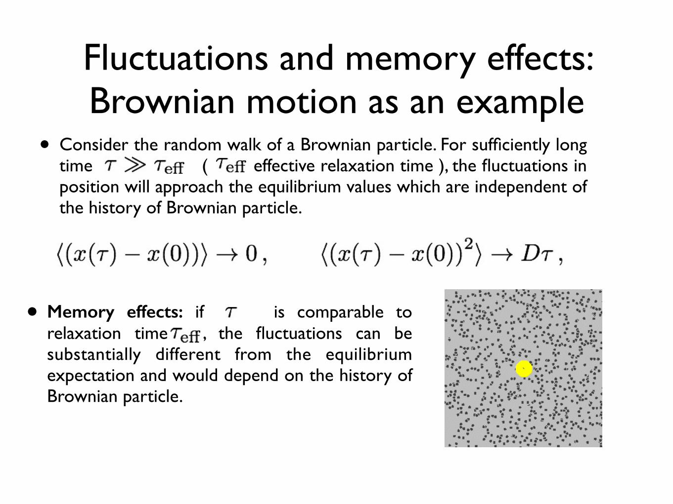
Fluctuations and memory effects: Brownian motion as an example

• Consider the random walk of a Brownian particle. For sufficiently long time ( effective relaxation time ), the fluctuations in position will approach the equilibrium values which are independent of the history of Brownian particle.

• Memory effects: if is comparable to relaxation time , the fluctuations can be substantially different from the equilibrium expectation and would depend on the history of Brownian particle.

Memory e↵ects of critical fluctuations

The relaxation time of critical mode also grows with correlationlength:

⌧e↵

⇠ ⇠z ,

with z defines the dynamical scaling exponent and z ⇠ 3 forQCD critical point.

⌧e↵

can be comparable or even larger than the time fireballspent in critical regime.

Knowledge of equilibrium fluctuations might not be su�cient.Memory e↵ects are important for understanding critical fluctu-ation in experiment.NB: as the sign of non-Gaussian cumulants can be either pos-itive or negative, even a qualitative understanding of their be-haviors in experiments requires taking memory e↵ects into ac-count!

Y.Y. Cumulants Evolution

This talk

• Understand how memory effects would affect the evolution of non-Gaussian cumulants.

• Understand the implication of such memory effects for detecting QCD critical point.

The evolution equations for cumulants

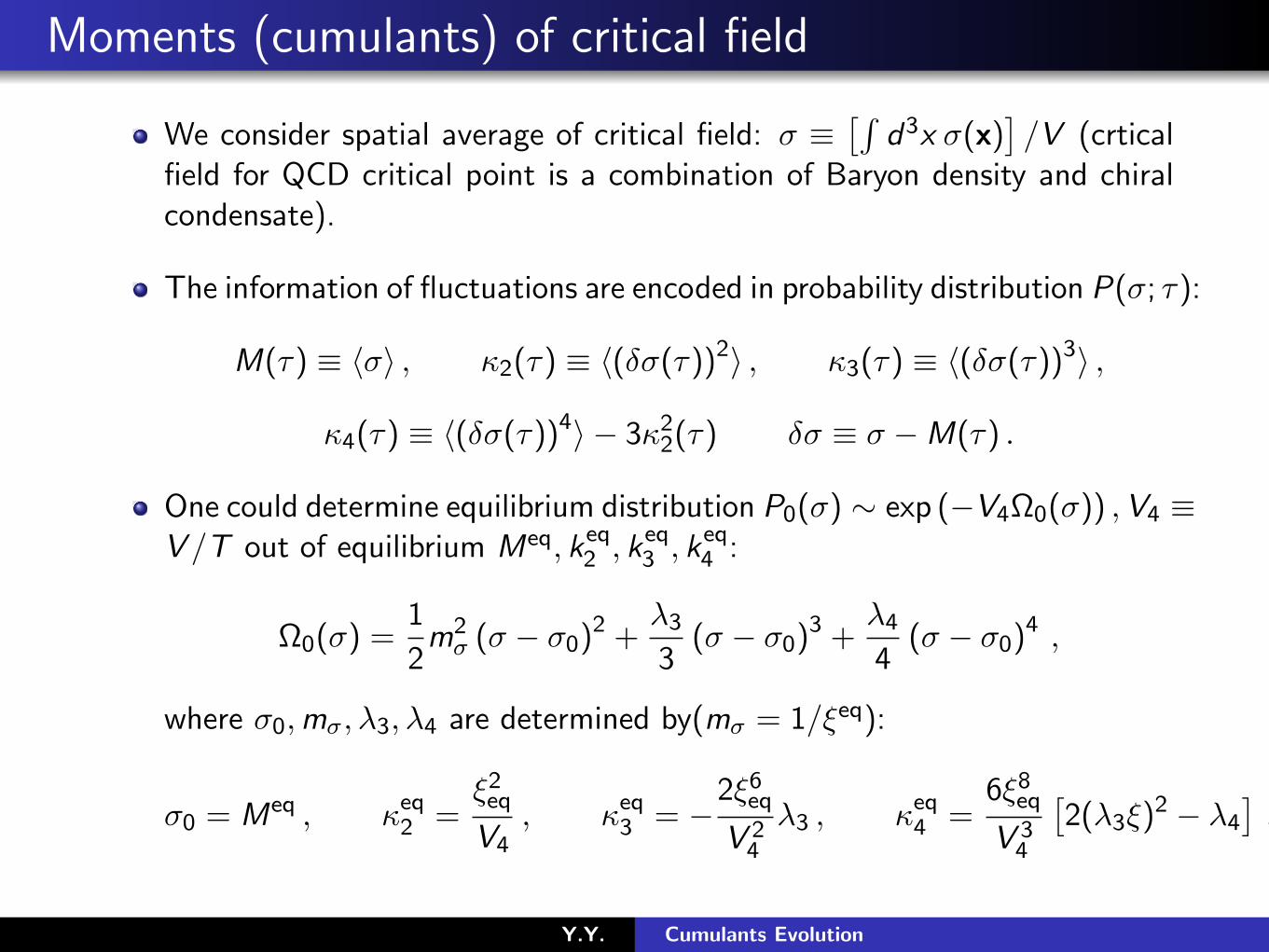
Moments (cumulants) of critical field

We consider spatial average of critical field: � ⌘ ⇥Rd

3

x �(x)⇤/V (crtical

field for QCD critical point is a combination of Baryon density and chiralcondensate).

The information of fluctuations are encoded in probability distribution P(�; ⌧):

M(⌧) ⌘ h�i , 2

(⌧) ⌘ h(��(⌧))2i , 3

(⌧) ⌘ h(��(⌧))3i ,

4

(⌧) ⌘ h(��(⌧))4i � 322

(⌧) �� ⌘ � �M(⌧) .

One could determine equilibrium distribution P0

(�) ⇠ exp (�V

4

⌦0

(�)) ,V4

⌘V /T out of equilibrium M

eq, keq2

, keq3

, keq4

:

⌦0

(�) =1

2m

2

� (� � �0

)2 +�3

3(� � �

0

)3 +�4

4(� � �

0

)4 ,

where �0

,m�,�3

,�4

are determined by(m� = 1/⇠eq):

�0

= M

eq , eq2

=⇠2eq

V

4

, eq3

= �2⇠6eq

V

2

4

�3

, eq4

=6⇠8

eq

V

3

4

⇥2(�

3

⇠)2 � �4

⇤,

Y.Y. Cumulants Evolution

The evolution of non-equilibrium cumulants

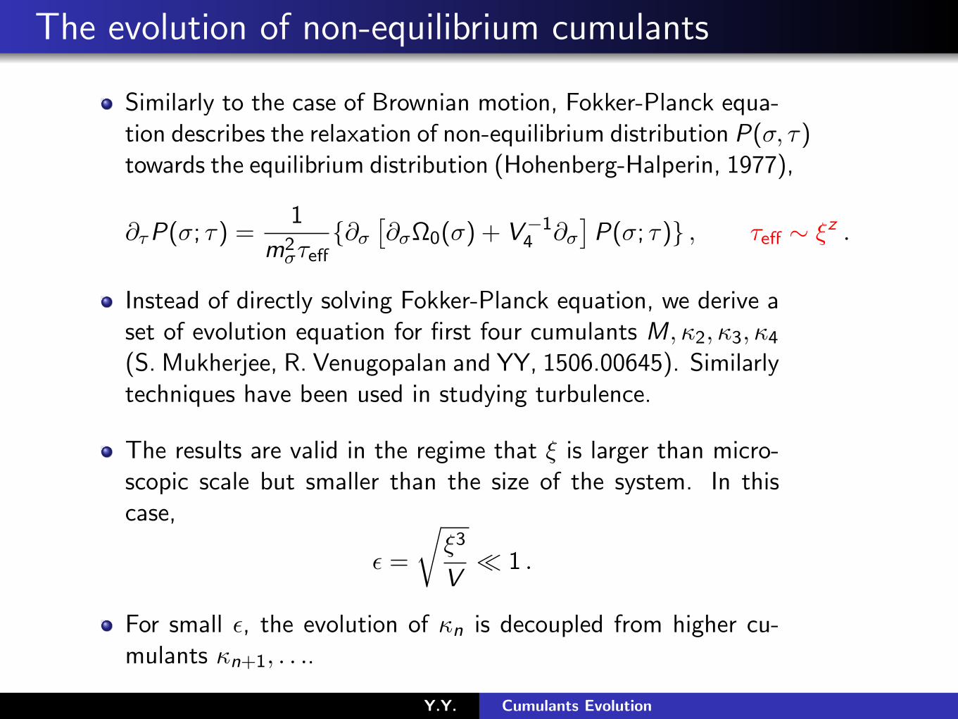
Similarly to the case of Brownian motion, Fokker-Planck equa-tion describes the relaxation of non-equilibrium distribution P(�, ⌧)towards the equilibrium distribution (Hohenberg-Halperin, 1977),

@⌧P(�; ⌧) =1

m

2

�⌧e↵{@�

⇥@�⌦0

(�) + V

�1

4

@�⇤P(�; ⌧)} , ⌧

e↵

⇠ ⇠z .

Instead of directly solving Fokker-Planck equation, we derive aset of evolution equation for first four cumulants M,

2

,3

,4

(S. Mukherjee, R. Venugopalan and YY, 1506.00645). Similarlytechniques have been used in studying turbulence.

The results are valid in the regime that ⇠ is larger than micro-scopic scale but smaller than the size of the system. In thiscase,

✏ =

r⇠3

V

⌧ 1 .

For small ✏, the evolution of n is decoupled from higher cu-mulants n+1

, . . ..

Y.Y. Cumulants Evolution

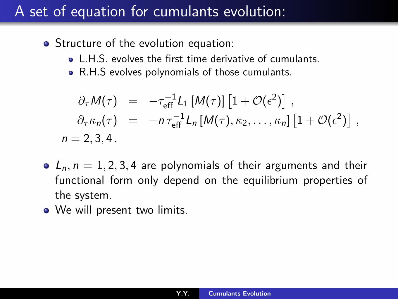
A set of equation for cumulants evolution:

Structure of the evolution equation:L.H.S. evolves the first time derivative of cumulants.R.H.S evolves polynomials of those cumulants.

@⌧M(⌧) = �⌧�1

e↵

L

1

[M(⌧)]⇥1 +O(✏2)

⇤,

@⌧n(⌧) = �n ⌧�1

e↵

Ln [M(⌧),2

, . . . ,n]⇥1 +O(✏2)

⇤,

n = 2, 3, 4 .

Ln, n = 1, 2, 3, 4 are polynomials of their arguments and theirfunctional form only depend on the equilibrium properties ofthe system.We will present two limits.

Y.Y. Cumulants Evolution

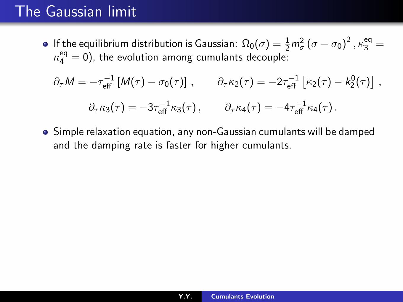
The Gaussian limit

If the equilibrium distribution is Gaussian: ⌦0

(�) = 1

2

m

2

� (� � �0

)2 ,eq3

=eq4

= 0), the evolution among cumulants decouple:

@⌧M = �⌧�1

e↵

[M(⌧)� �0

(⌧)] , @⌧2(⌧) = �2⌧�1

e↵

⇥2

(⌧)� k

0

2

(⌧)⇤,

@⌧3(⌧) = �3⌧�1

e↵

3

(⌧) , @⌧4(⌧) = �4⌧�1

e↵

4

(⌧) .

Simple relaxation equation, any non-Gaussian cumulants will be dampedand the damping rate is faster for higher cumulants.

Y.Y. Cumulants Evolution

Near equilibrium limit

If the deviation from equilibrium of cumulants is small �n ⌘n � eqn , evolution equation is linearized:

@⌧M(⌧) = �⌧�1

e↵

�M , @⌧2(⌧) = �2 ⌧�1

e↵

�̃2

,

@⌧3(⌧) = �3 ⌧�1

e↵

(✏b3)

✓�

3

✏b3

◆+ 4�̃

3

✓�

2

b

2

◆�,

@⌧ [4(⌧)] = �4 ⌧�1

e↵

(✏2b4)

( ✓�

4

✏2b4

◆+ 6�̃

3

✓�

3

✏b3

◆

� 6⇣2�̃2

3

� 3�̃4

⌘✓�

2

b

2

◆).

The evolution of higher cumulants are coupled to lower ones.Lower moments will be relaxed back to the equilibrium first.

Y.Y. Cumulants Evolution

Summary of Part I:

• We have derived a set of equations for the evolution of cumulants.

• We now apply it to the QCD critical regime. (We will restrict ourselves to the cross-over side of critical regime as effects such as bubble nucleation are not incorporated in the present approach.)

Evolution of cumulants in QCD critical regime.

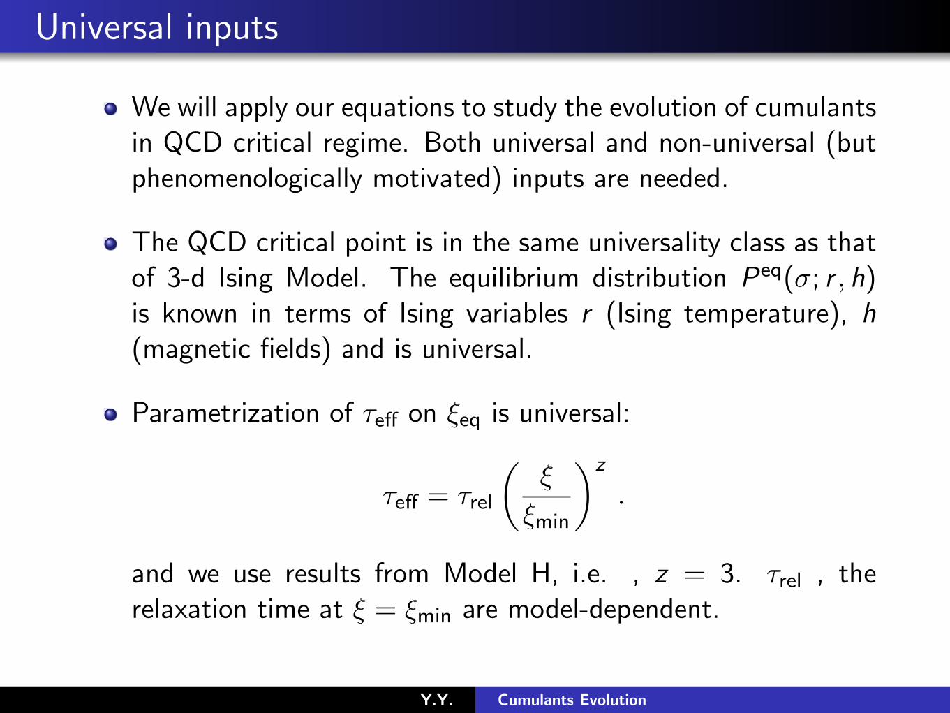
Universal inputs

We will apply our equations to study the evolution of cumulantsin QCD critical regime. Both universal and non-universal (butphenomenologically motivated) inputs are needed.

The QCD critical point is in the same universality class as thatof 3-d Ising Model. The equilibrium distribution P

eq(�; r , h)is known in terms of Ising variables r (Ising temperature), h(magnetic fields) and is universal.

Parametrization of ⌧e↵

on ⇠eq

is universal:

⌧e↵

= ⌧rel

✓⇠

⇠min

◆z

.

and we use results from Model H, i.e. , z = 3. ⌧rel

, therelaxation time at ⇠ = ⇠

min

are model-dependent.

Y.Y. Cumulants Evolution

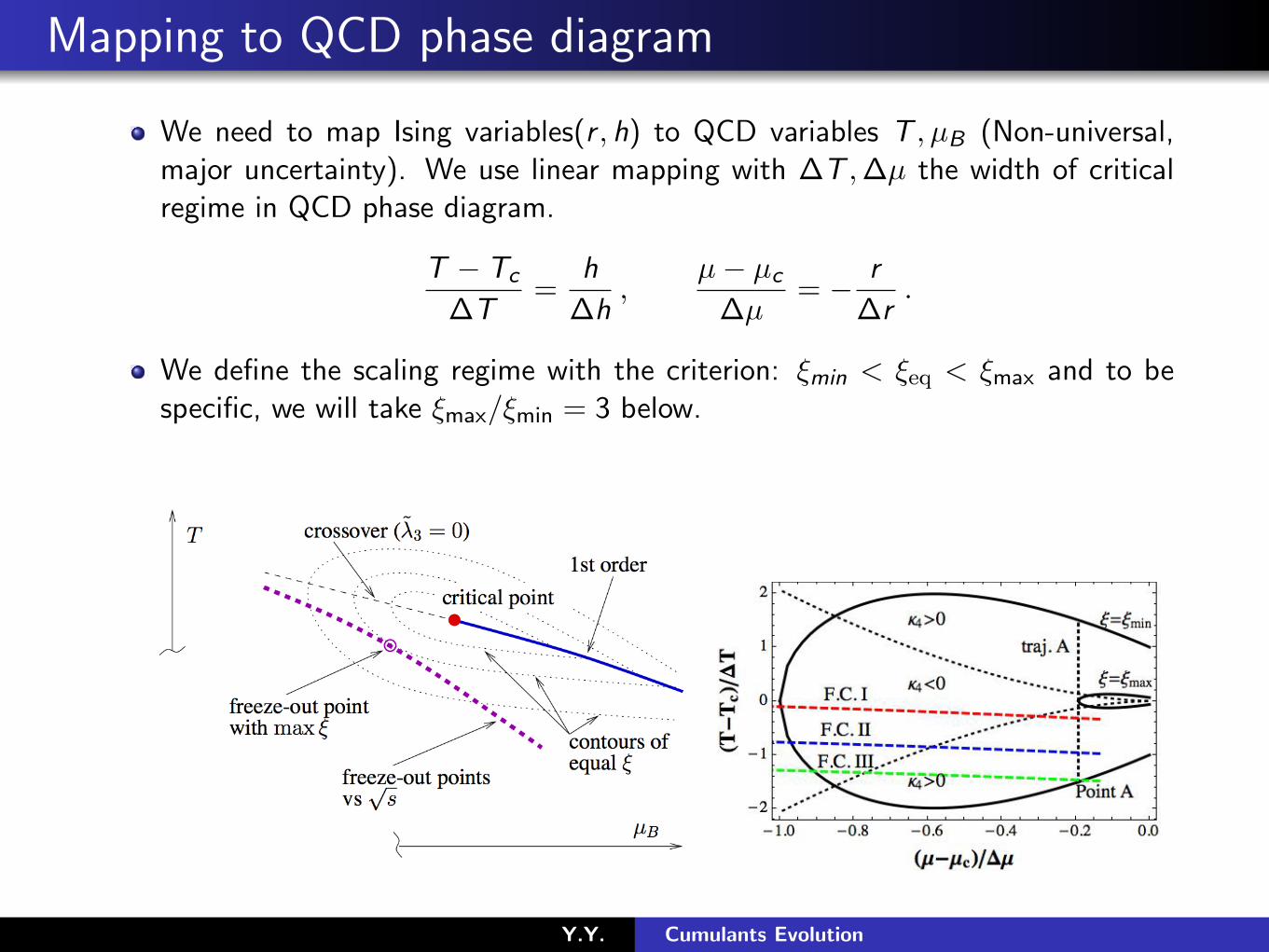
Mapping to QCD phase diagram

We need to map Ising variables(r , h) to QCD variables T , µB (Non-universal,major uncertainty). We use linear mapping with �T ,�µ the width of criticalregime in QCD phase diagram.

T � Tc

�T

=h

�h

,µ� µc

�µ= � r

�r

.

We define the scaling regime with the criterion: ⇠min < ⇠eq < ⇠max

and to bespecific, we will take ⇠

max

/⇠min

= 3 below.

Y.Y. Cumulants Evolution

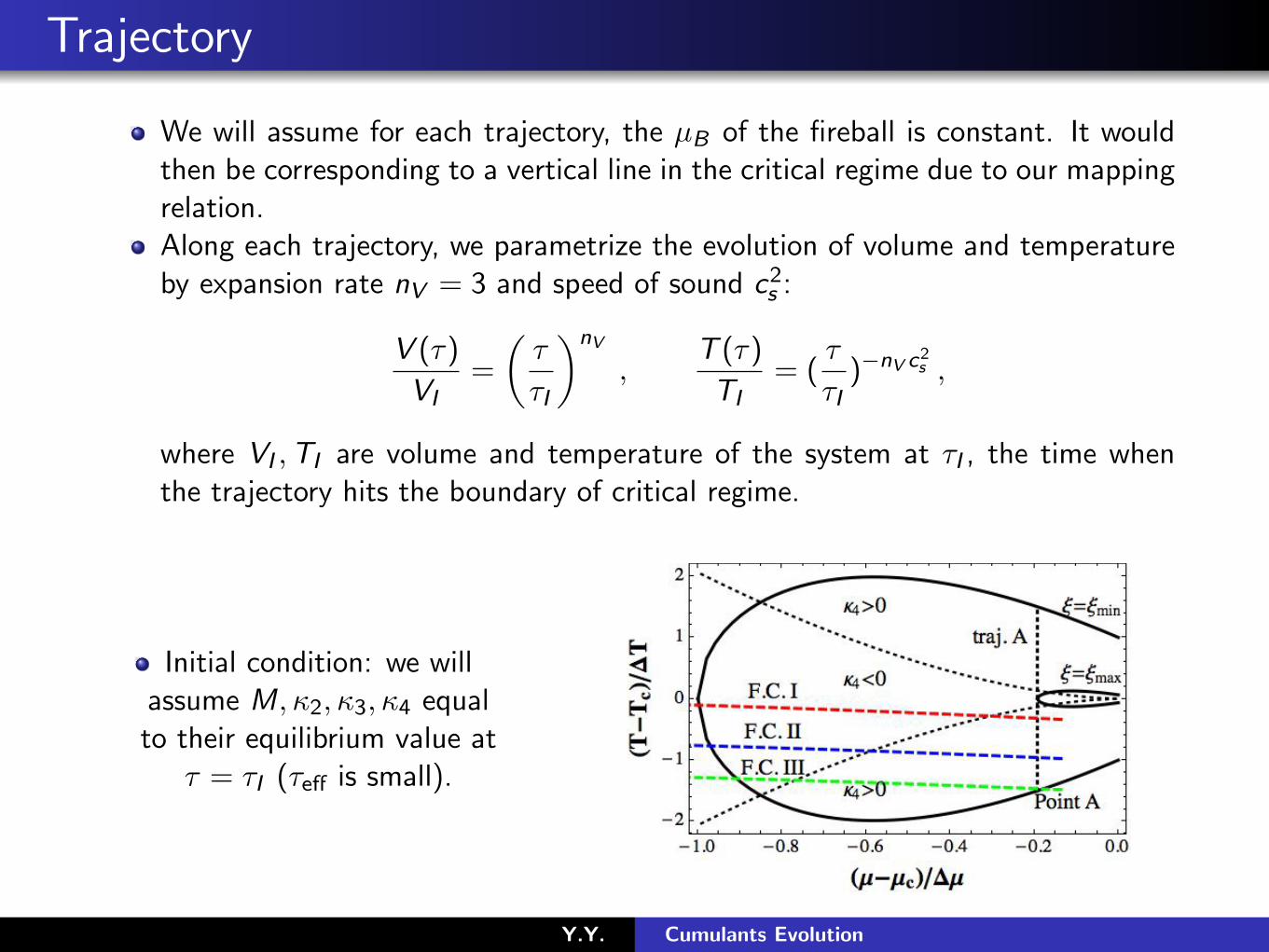
Trajectory

We will assume for each trajectory, the µB of the fireball is constant. It wouldthen be corresponding to a vertical line in the critical regime due to our mappingrelation.Along each trajectory, we parametrize the evolution of volume and temperatureby expansion rate nV = 3 and speed of sound c

2

s :

V (⌧)

VI=

✓⌧

⌧I

◆nV

,T (⌧)

TI= (

⌧

⌧I)�nV c2s ,

where VI ,TI are volume and temperature of the system at ⌧I , the time whenthe trajectory hits the boundary of critical regime.

Initial condition: we willassume M,

2

,3

,4

equalto their equilibrium value at

⌧ = ⌧I (⌧e↵ is small).

Y.Y. Cumulants Evolution

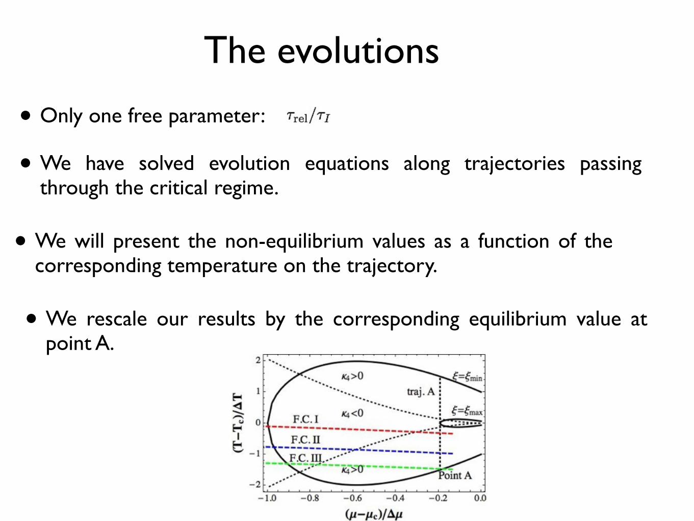
The evolutions

• We will present the non-equilibrium values as a function of the corresponding temperature on the trajectory.

• We have solved evolution equations along trajectories passing through the critical regime.

• We rescale our results by the corresponding equilibrium value at point A.

• Only one free parameter:

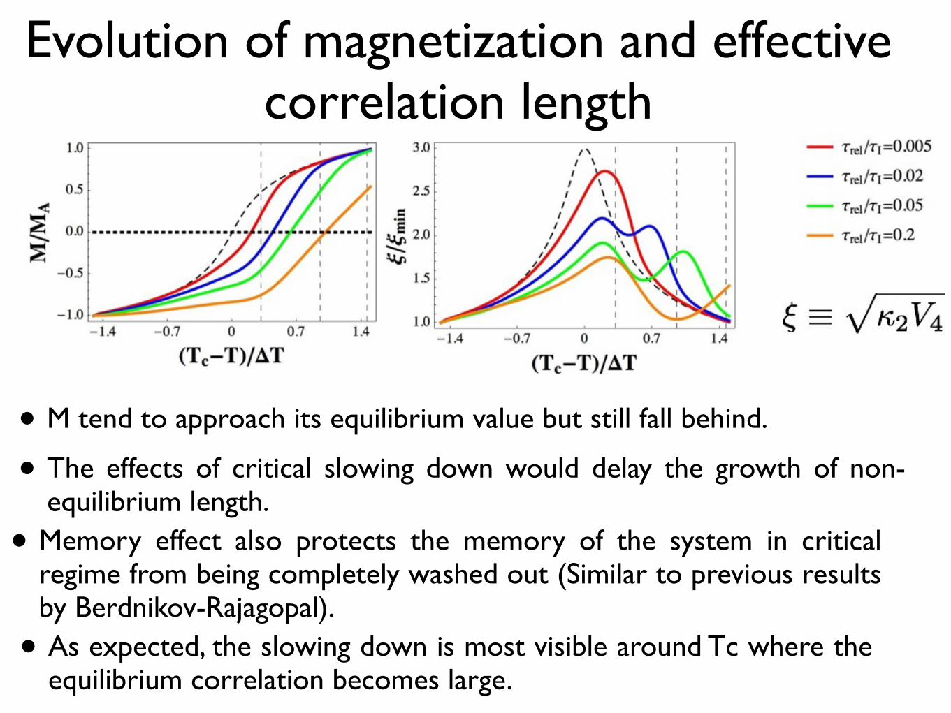
Evolution of magnetization and effective correlation length

• The effects of critical slowing down would delay the growth of non-equilibrium length.

• M tend to approach its equilibrium value but still fall behind.

• As expected, the slowing down is most visible around Tc where the equilibrium correlation becomes large.

• Memory effect also protects the memory of the system in critical regime from being completely washed out (Similar to previous results by Berdnikov-Rajagopal).

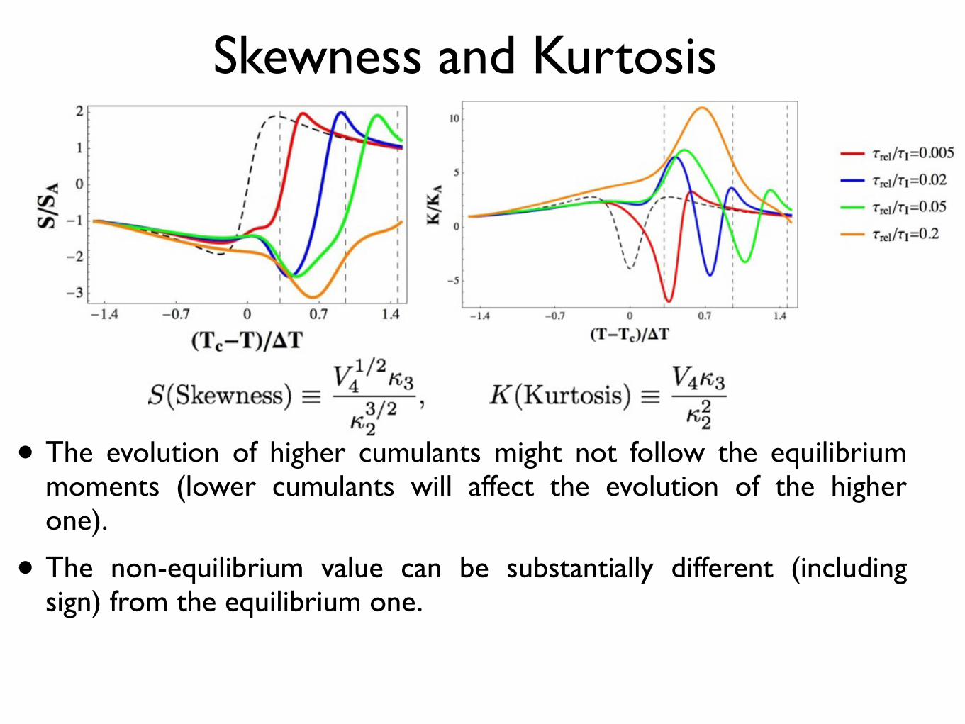
Skewness and Kurtosis

• The evolution of higher cumulants might not follow the equilibrium moments (lower cumulants will affect the evolution of the higher one).

• The non-equilibrium value can be substantially different (including sign) from the equilibrium one.

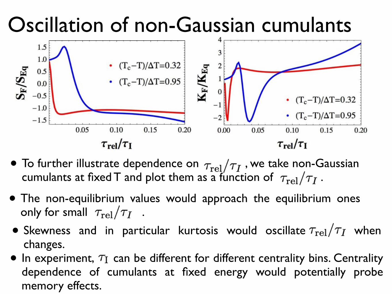
Oscillation of non-Gaussian cumulants

• To further illustrate dependence on , we take non-Gaussian cumulants at fixed T and plot them as a function of .

• The non-equilibrium values would approach the equilibrium ones only for small .

• Skewness and in particular kurtosis would oscillate when changes.

• In experiment, can be different for different centrality bins. Centrality dependence of cumulants at fixed energy would potentially probe memory effects.

Part III: Implications on BES and the search for QCD critical point

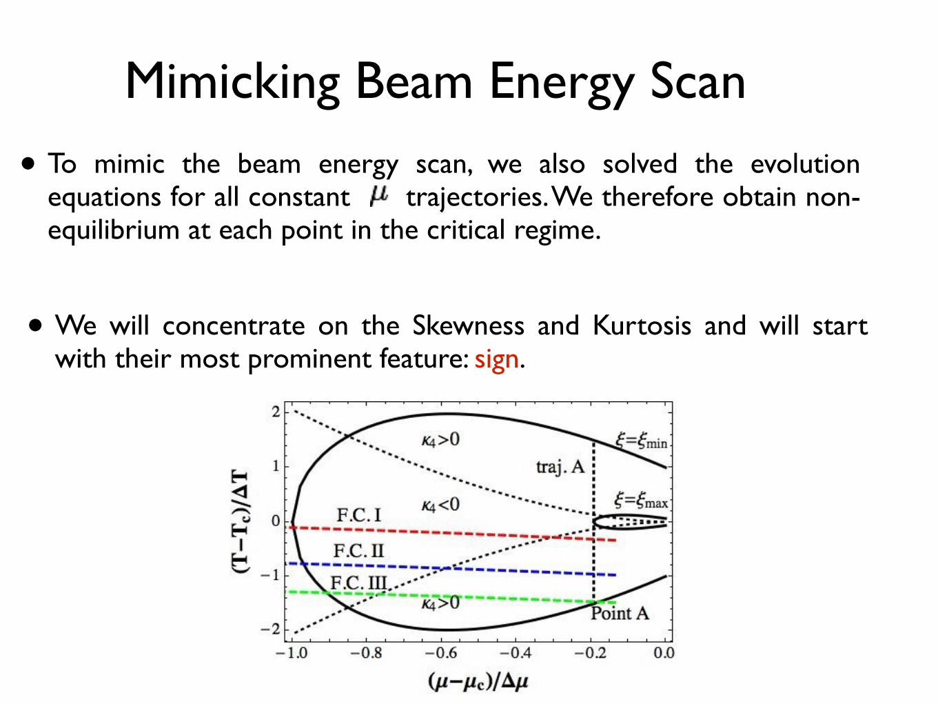
Mimicking Beam Energy Scan

• To mimic the beam energy scan, we also solved the evolution equations for all constant trajectories. We therefore obtain non-equilibrium at each point in the critical regime.

• We will concentrate on the Skewness and Kurtosis and will start with their most prominent feature: sign.

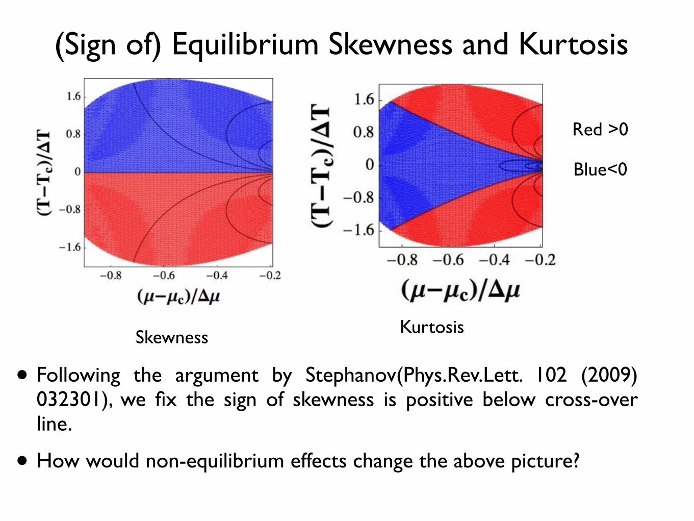
(Sign of) Equilibrium Skewness and Kurtosis

• Following the argument by Stephanov(Phys.Rev.Lett. 102 (2009) 032301), we fix the sign of skewness is positive below cross-over line.

Skewness Kurtosis

Red >0

Blue<0

• How would non-equilibrium effects change the above picture?

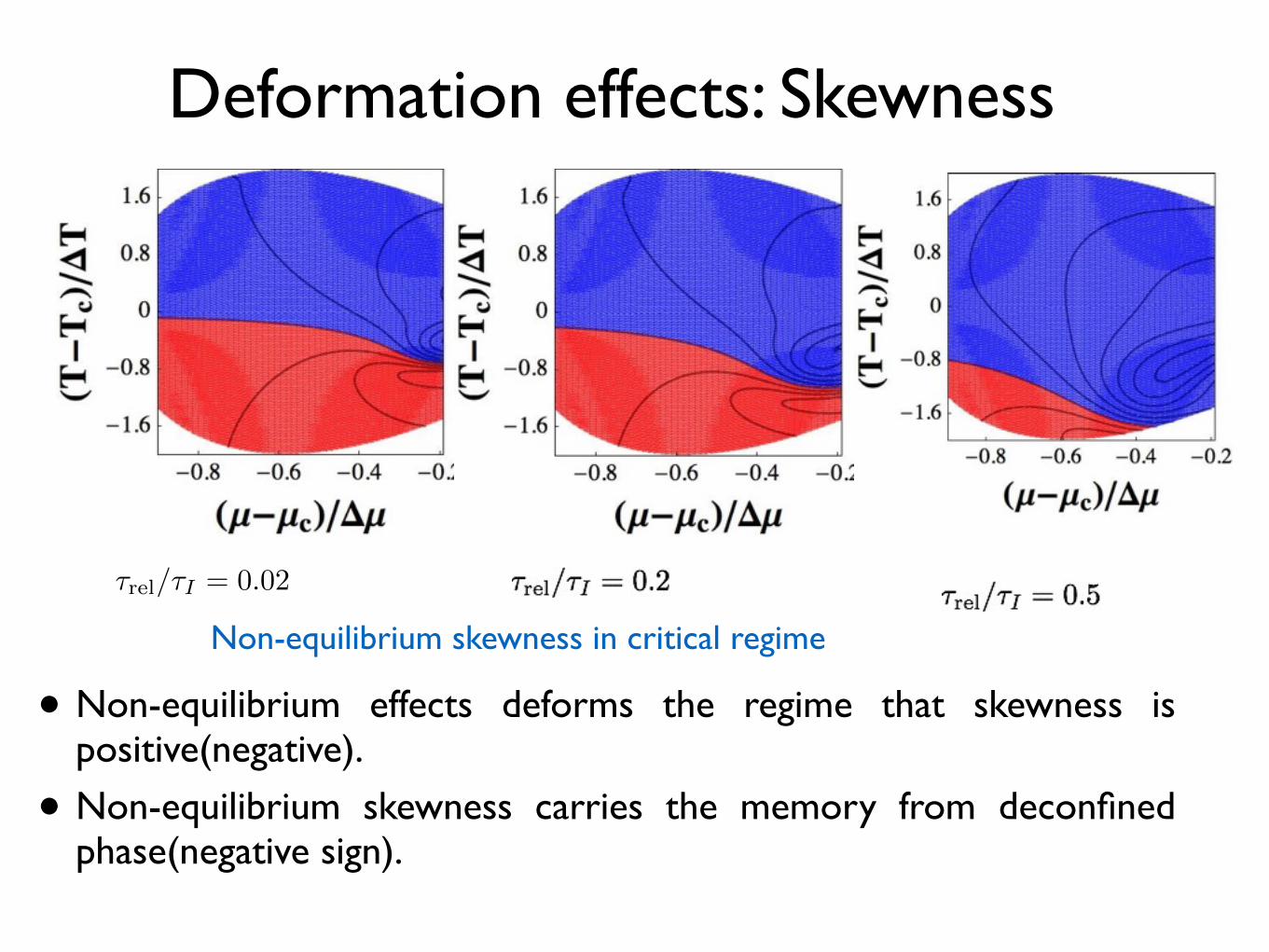
Deformation effects: Skewness

• Non-equilibrium effects deforms the regime that skewness is positive(negative).

• Non-equilibrium skewness carries the memory from deconfined phase(negative sign).

⌧rel/⌧I = 0.02

Non-equilibrium skewness in critical regime

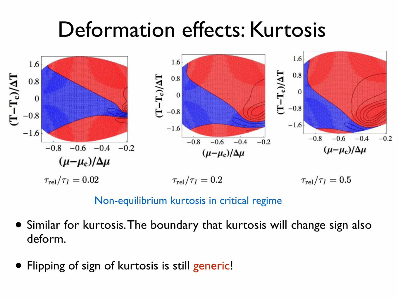
Deformation effects: Kurtosis

• Similar for kurtosis. The boundary that kurtosis will change sign also deform.

Non-equilibrium kurtosis in critical regime

• Flipping of sign of kurtosis is still generic!

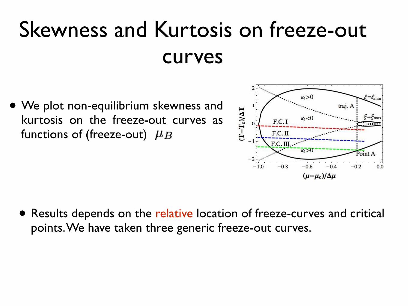
Skewness and Kurtosis on freeze-out curves

• Results depends on the relative location of freeze-curves and critical points. We have taken three generic freeze-out curves.

• We plot non-equilibrium skewness and kurtosis on the freeze-out curves as functions of (freeze-out)

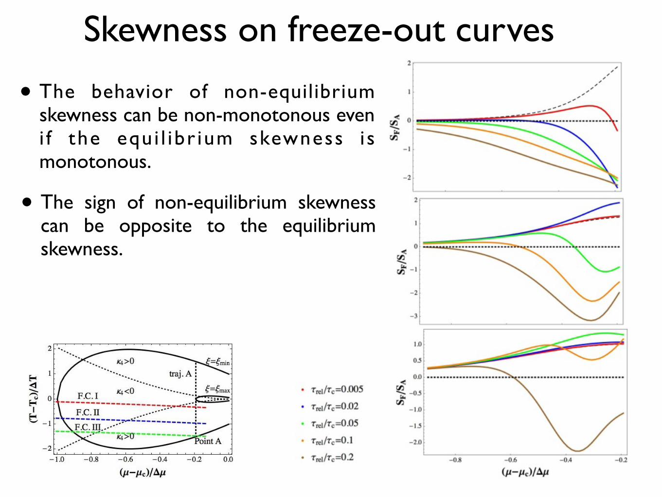
Skewness on freeze-out curves

• The sign of non-equilibrium skewness can be opposite to the equilibrium skewness.

• The behavior of non-equilibrium skewness can be non-monotonous even i f the equ i l ibr ium skewness i s monotonous.

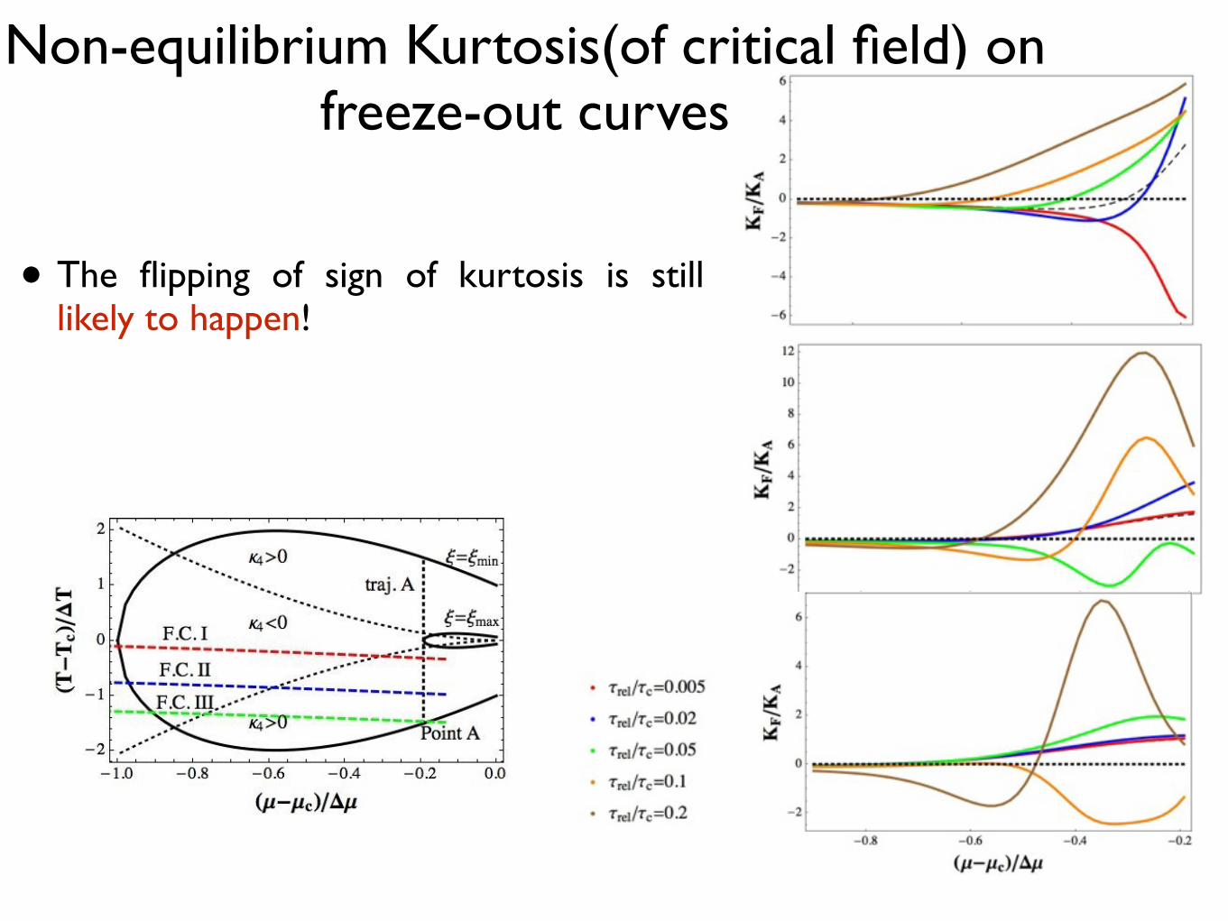
Non-equilibrium Kurtosis(of critical field) on freeze-out curves

• The flipping of sign of kurtosis is still likely to happen!

• Different combination of the relative locations of freeze-out curves and relaxation time would give similar trend.

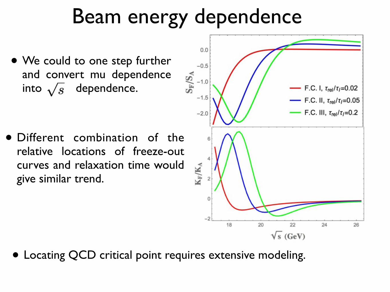
Beam energy dependence

• We could to one step further and convert mu dependence into dependence.

• Locating QCD critical point requires extensive modeling.

Summary

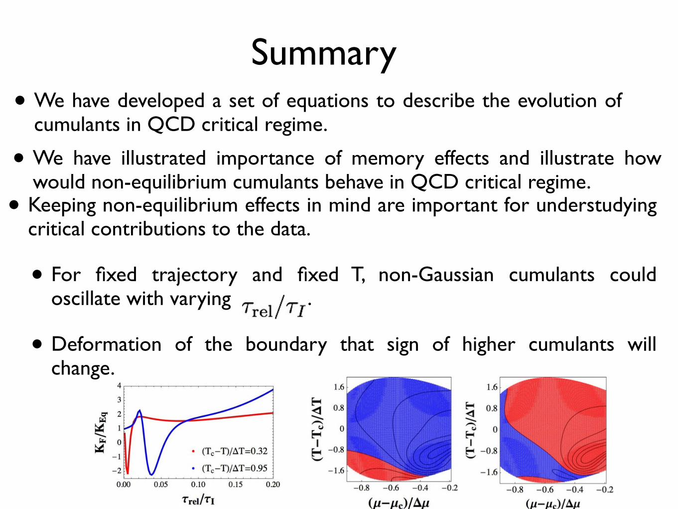
Summary • We have developed a set of equations to describe the evolution of

cumulants in QCD critical regime.

• We have illustrated importance of memory effects and illustrate how would non-equilibrium cumulants behave in QCD critical regime.

• Keeping non-equilibrium effects in mind are important for understudying critical contributions to the data.

• For fixed trajectory and fixed T, non-Gaussian cumulants could oscillate with varying .

• Deformation of the boundary that sign of higher cumulants will change.