The Quantitative Role of Child Care for Fertility

and Female Labor Force Participation

Alexander Bick∗

Goethe University, Frankfurt

February 15, 2010

Abstract

This paper documents facts about labor force participation and child careenrollment decisions of married females in West Germany. In line withthe facts for a cross-section of OECD countries, a special emphasis is puton the level relationship between maternal labor force participation andchild care enrollment. A calibrated life-cycle model is used to evaluatethe quantitative impact of providing (subsidized) child care on maternallabor force participation and fertility.

Keywords: Child Care, Fertility, Life-cycle Female Labor Supply

JEL classification: J12, D91

∗I am indebted to Dirk Krueger for his guidance and advise at all stages of this project. Ithank Sekyu Choi, Nicola Fuchs-Schundeln, Jorgo Georgiadis, Jeremy Greenwood, Fane NajaGroes, Bertrand Gobillard, John Knowles, Alexander Ludwig, Petra Todd and Ken Wolpinfor helpful discussions. I also would like thank seminar participants at the Universities ofCopenhagen, Frankfurt, Mannheim and Pennsylvania for helpful comments and suggestions.This research is supported by the Cluster of Excellence “Normative Orders” at Goethe Uni-versity, Frankfurt. Part of this paper was written during a visit at the Economics Departmentat the University of Pennsylvania, Philadelphia. I want to thank for their hospitality and theGerman Academic Exchange Service (DAAD) for financial support. E-mail: bick@wiwi.uni-frankfurt.de

1 Introduction

“Member States should remove disincentives for female labour force

participation and strive, in line with national patterns of provision,

to provide childcare by 2010 to at least 90% of children between 3years old and the mandatory school age and at least 33% of children

under 3 years of age.”

European Council Barcelona - Conclusions of the Presidency (2002)

According to the above quote, the lack of provision of child care is at leastby EU politicians perceived as one of the main disincentives for female laborforce participation. Indeed, the enrollment rate in child care of children belowage three and the corresponding maternal labor force participation rate aresignificantly, positively correlated, see the left panel of Figure 1.

Figure 1: Child Care Enrollment of Children Aged 0 to 2 in the OECD

CZ

IT

AT

HU

GR

LUIE

JPSK

CA

ES

PT

UKFRAU

NL

NZ

BE

FIUSA

SW

IS

DK

West Germany

010

2030

4050

6070

8090

100

Mat

erna

l Lab

or F

orce

Par

ticip

atio

n R

ate

0 10 20 30 40 50 60 70 80 90 100Child Care Enrollment Rate

Fit 45 Degree Line

Maternal Labor Force Participation

PLCZ

MX

ITAT

HUGR

LU

IE

JPSK

CA

ROK

ESPT

UK

FR

AU

NL

NZ

BE

FI

USA

SWNO

IS

DK

West Germany

1.1

1.3

1.5

1.7

1.9

2.1

2.3

Tot

al F

ertil

ity R

ate

0 10 20 30 40 50 60 70 80 90 100Child Care Enrollment Rate

Fit

Fertility

Source: OECD (2005), own calculations

As a matter of fact, the right panel of Figure 1 shows a significant positivecorrelation between the child care enrollment rate of children below age threeand the total fertility rate – a further motivation for the interest in child caregiven the below replacement fertility rates in most European countries. In thelight of the demographic change and the financing of the pay-as-you-go socialsecurity systems, both larger female labor force participation rates and higherfertility rates seem to be desirable.

While these facts seem supportive for the above stated quote, two concernsmay be raised. First, despite the significant positive correlation for childrenbelow age three between the maternal labor force participation rate and childcare enrollment rate, the latter exceeds the former by an order of magnitude.

1

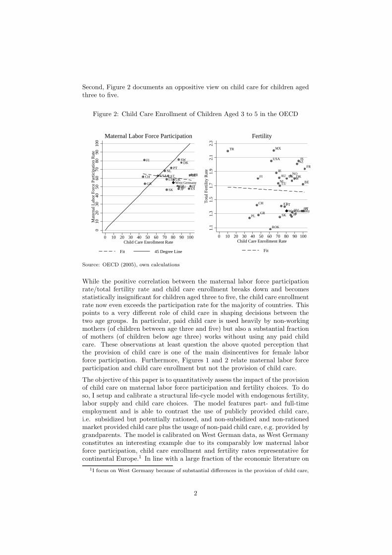
Second, Figure 2 documents an oppositive view on child care for children agedthree to five.

Figure 2: Child Care Enrollment of Children Aged 3 to 5 in the OECD

CH

FI

GR

USANL

LU

SK

AT

PT

UK

CZJP

SW

HU

DK

ES

BE

IT

FR

West Germany

010

2030

4050

6070

8090

100

Mat

erna

l Lab

or F

orce

Par

ticip

atio

n R

ate

0 10 20 30 40 50 60 70 80 90 100Child Care Enrollment Rate

Fit 45 Degree Line

Maternal Labor Force Participation

TR

PL

CH

FI

GR

ROK

USA

MX

IE

NL

AU

LU

SK

ATPT

UKNO

CZJP

SW

HU

DK

NZIS

ES

BE

IT

FR

West Germany1.

11.

31.

51.

71.

92.

12.

3T

otal

Fer

tility

Rat

e

0 10 20 30 40 50 60 70 80 90 100Child Care Enrollment Rate

Fit

Fertility

Source: OECD (2005), own calculations

While the positive correlation between the maternal labor force participationrate/total fertility rate and child care enrollment breaks down and becomesstatistically insignificant for children aged three to five, the child care enrollmentrate now even exceeds the participation rate for the majority of countries. Thispoints to a very different role of child care in shaping decisions between thetwo age groups. In particular, paid child care is used heavily by non-workingmothers (of children between age three and five) but also a substantial fractionof mothers (of children below age three) works without using any paid childcare. These observations at least question the above quoted perception thatthe provision of child care is one of the main disincentives for female laborforce participation. Furthermore, Figures 1 and 2 relate maternal labor forceparticipation and child care enrollment but not the provision of child care.

The objective of this paper is to quantitatively assess the impact of the provisionof child care on maternal labor force participation and fertility choices. To doso, I setup and calibrate a structural life-cycle model with endogenous fertility,labor supply and child care choices. The model features part- and full-timeemployment and is able to contrast the use of publicly provided child care,i.e. subsidized but potentially rationed, and non-subsidized and non-rationedmarket provided child care plus the usage of non-paid child care, e.g. provided bygrandparents. The model is calibrated on West German data, as West Germanyconstitutes an interesting example due to its comparably low maternal laborforce participation, child care enrollment and fertility rates representative forcontinental Europe.1 In line with a large fraction of the economic literature on

1I focus on West Germany because of substantial differences in the provision of child care,

2

female labor supply, I focus in the empirical and quantitative analysis on femalesin stable, long-term relationships. While this might reduce the generality ofthe results, the analyzed group is from a policy perspective one of the mostinteresting ones. First, given the spousal income, they are the least likely towork. Second, females in stable, long-term relationships have above averagefertility rates. In both cases, the response to changes in the provision of childcare most likely constitutes a lower bound on responses of the population offemales.

A number of recent papers investigates the quantitative importance of childcare using structural models, all with the application to Germany. However,in contrast to this paper, the existing literature about life-cycle models withfertility choices and female labor force participation either does not model fer-tility jointly as a choice and/or requires females for each hour of work to buyone hour of child care, which is as shown in Figure 1 at odds with the data.The paper of Domeij and Klein (2009) is subject to both shortcomings althoughtheir model allows to point out some important optimal taxation considera-tions. Haan and Wrohlich (2009) estimate a structural, empirical micro modelwith endogenous fertility, but also require the strict substitution between femalehours worked and usage of child care. Since most of the working West Germanmothers with children below age three do not use any paid child care at all,the policy implications of the results in Domeij and Klein (2009) and Haan andWrohlich (2009) might be flawed by the inappropriate role attributed to paidchild care. Wrohlich (2006) circumvents this problem by taking the option ofnon-paid child care explicitly into account, but does neither model fertility nordoes she consider a life-cycle setting.

The results of conducting a set of counterfactual policy experiments, mimickingrecently implemented or currently discussed policy reforms, can be summarizedas follows: the quantitative impact of providing (subsidized) child care on femalelabor force participation and fertility is very small whereas financial support tai-lored towards mothers of young children is more effective in stimulating fertilitywithout decreasing labor force participation in the long run.

The structure of the paper is as follows: In Section 2, I describe the data set, andhow the sample is selected and constructed. Section 3 documents facts about thesupply of paid child care, female labor force participation and child care usagein West Germany. I introduce the model in Section 4 and discuss the calibrationand model fit in Section 5. In Sections 6 conduct a set of counterfactual policyexperiments and Section 7 concludes.

2 Data

In this Section I introduce the data set the analysis of female labor force partici-pation, child care and fertility in West Germany and briefly discuss the selectionand construction of the underlying sample.

originating from the pre-unification period but persisting until today, the labor market andfamily structure between West and East Germany.

3

2.1 German Socio-Economic Panel (GSOEP)

The GSOEP is an annual household panel, comparable in scope to the AmericanPSID. It is a representative longitudinal study of private households with thefirst survey having been conducted in 1984 for West Germany and in 1990 forEast Germany. New samples were added in 1994, 1998, 2000, 2002 and 2006.2

The variables I construct from the GSOEP include female cohabitation, femalelabor force participation and birth histories, child care usage, child care fees,and income profiles. The data are drawn from the 1984 to 2007 waves, andspan the years 1983 to 2006 since the variables on labor force participation andincome refer to the year prior to the interview.

2.2 Sample Selection

As in Francesconi (2002), only females living in a continuous relationship withthe same partner are included in the sample since many economic theories ofhousehold production, female labor supply, and fertility are meant to describebehavior of this group only.3 This might introduce a selection bias, if the un-observables affecting marriage stability are also correlated with the fertility andparticipation decisions.4 In this paper, I use marriage interchangeably with co-habitation because the interest is less on the legal status but rather on livingin a relationship in one household. Females with multiple relationships over theobservation period enter the data set only with their most recent one and if itis still intact at the last interview. Among mothers, only those are includedin the sample that have all children within the current marital spell, while forchildless females the requirement is that they were already in that spell priorto age forty and thus had (at least theoretically) the possibility to give birthto a child. Furthermore, I only consider females that lived in West Germanythroughout the whole observation period to ensure that all females in the sam-ple faced the same economic environment.5 Finally, given a trade-off between asufficient sample size and homogenous sample of females with respect to birthyears only females born between 1955 and 1975 are included. The number ofindividuals satisfying the respective selection criteria are shown in Table 17 inAppendix.

2Detailed information about the GSOEP are provided on the corresponding webpagehttp://www.diw.de/english/soep/26636.html.

3For a survey on fertility theories for married females see e.g. Jones et al. (2008). Recentcontributions also model fertility, marriage and divorce jointly, e.g. Regalia and Rios-Rull(2001) or Greenwood et al. (2003).

4The direction of the sample selection bias with respect to labor force participation andfertility can go in either direction. For a detailed discussion, see Francesconi (2002) pp 347f.

5Females are assigned to West Germany by their location in 1989 or, if this information isnot available, by the sample region at their first interview.

4

2.3 Sample Construction

2.3.1 Period Definition

Female labor force participation profiles along children’s age constitute the coreof the analysis in this paper. Similarly to Apps and Rees (2005), my focus isless on the participation status in each month of a child’s life but rather on thestages during a child’s adolescence, see Figure 3.

Figure 3: A Child’s Life from Birth to Adulthood

Pre-school School

Age

Period

0 3 6.5 9.5 12.5 15.5 18.5

1 2 3 4 5 6

The first two periods comprise the pre-schooling years with age six and a half asthe mean age at school entry. The third period refers to grades one to three in el-ementary school (Grundschule), while the fourth period comprises fourth gradeof elementary school plus grades five and six of secondary school (Forderstufe orUnterstufe). After the fifth period, teenagers can already graduate (Hauptschu-labschluss) and start an apprenticeship or continue to attend school until theyreach adulthood at the end of period six. All periods have a length of threeyears with the exception of period two which has a mean of three years.6

2.3.2 Labor Supply

For each period the female labor supply and child care enrollment status isconstructed similar to Francesconi (2002): I assign “0” to each month in whichthe female does not work, “0.5” to each month in which she works part-time and“1” to each month in which she works full-time.7 Next, the mean over all monthsin a period is taken defining the period labor supply status. Values below 0.25correspond to not working, values between 0.25 and 0.75 to part-time working,and values above 0.75 to full-time working. This assignment implies that afemale working part-time in each month of the period and one not working inthe first half of a period but full-time in the second half have the same periodlabor supply status, namely part-time working. As already mentioned before,this reflects how much a female has worked in total in certain stages during herchildren’s adolescence.

6Details on the first two periods are given in Appendix A.1.1.7The monthly labor force participation status is based on the retrospective infor-

mation for the previous year at each interview months. I follow the convention inhttp://www.diw.de/documents/dokumentenarchiv/17/60055/pgen.pdf for the classificationof part- and full-time work.

5

2.3.3 Child Care

In the introductory quote, the European Council instructed member states ofthe EU to meet certain targets of child care provision. I define publicly providedchild care as follows. The GSOEP asks for two different categories of child care,namely daycare centers and nannies. Since, in contrast to nannies, 95% of alldaycare centers receive public subsidies I use this category for publicly providedchild care, henceforth called subsidized child care, whereas nannies are labeled asnon-subsidized child care, reflecting a market arrangement. This categorizationis in line with Wrohlich (2006) and Haan and Wrohlich (2009). Two limitationsin the GSOEP are relevant for this paper. First, prior to 1995, the questionnaireonly covered enrollment in child care whereas from 1995 onwards a distinctionbetween daycare centers and nannies was made. In particular, between 1995 and1999 the distinction between daycare centers and nannies was exclusive and from2000 onwards non-exclusive. Furthermore, for care provided by nannies from2004 onwards part- and full-time can not be distinguished anymore. I thereforeonly calculate the following two variables. Child care enrollment comprisingsubsidized (daycare centers) and non-subsidized (nannies) child care for all yearswhich can be part- or full-time, and from the year 1995 onwards the fraction ofchildren enrolled in non-subsidized child care (nannies) from all children enrolledin child care (daycare centers and/or nannies). The second limitation of theGSOEP relevant for this paper is that information on child care enrollment isonly available for the interview date. In Appendix A.1.2 I describe how I imputethe child care enrollment status for the remaining months of a year. The periodchild care enrollment status is then calculated in the same way as for laborsupply.

One specific characteristic of subsidized child care, i.e. child care provided indaycare centers, is a limited number of available slots. Based on data fromthe German Statistical Office for every fourth year between 1986 and 2002, Icompute the provision rate of subsidized part- and full-time slots per hundredchildren consistent with the definition used for the period labor force participa-tion and child care enrollment status, see Appendix A.1.2.

2.3.4 Period Assignment

If a female has more than one child, the life periods of siblings only overlapperfectly for twins or triplets. Females observed the last time prior to the endof their fertile period might give birth to another child. Therefore, the analysisof females with one child (two/three children) will be based on the decisions offemales after their first (second/third) birth until they are not observed anymoreor give birth to a second (third/fourth) child. Hence, a female who gives birthto two children during the observation period contributes to facts about femaleswith one child until the second child is born and to facts about females with twochildren afterwards. Moreover to avoid biased averages if there are trends inlabor participation or child care enrollment within a period, i.e. during a stageof a child’s adolescence, only periods that are neither interrupted by anotherbirth nor left or right censored through the first or last interview are included.

Recall that childless females are only included in the sample if they are observed

6

to reach at least age forty. I therefore assign the first three years of childlessfemales after turning forty to the first period, the next three and half years tothe second period and so forth.

2.4 Sample Size

Table 1 shows the number of observations for each period grouped by the numberof children, e.g. 389 females with one child that is younger than three and 181females with one child of age three to six and half are observed. Since there

Table 1: Distribution of Observations per Number of Children by Age

Age Number of childrenyoungest child 0 1 2 3 4+

< 3 68 400 458 126 39

< 6.5 38 186 332 99 27

< 9.5 14 131 274 85 30

< 12.5 0 111 212 59 15

< 15.5 0 86 129 38 8

< 18.5 0 64 106 22 8

Note: For childless females < 3 corresponds to femaleages 40 to 42, < 6.5 to 43 and 46.5 and so forth. Sincethe first birth cohort of females included in the samplewas born in 1945 and the last observations are from2006, childless females could only be observed for threeperiods.

are not sufficient females with zero or four and more children, the analysis onlabor force participation and child care enrollment in this paper will focus onfemales with one to three children only. The sample I use to calculate thefertility rate and distribution comprises all selected females who are at least ofage 40 at their last interview, even if they only have incomplete periods andthus do not contribute to the set of stylized facts about labor supply and childcare enrollment, and is restricted to females with zero to three children. Sincethe timing of birth is not part of the investigation in this paper, females not yethaving completed their fertile period, assumed to end at the age of forty, areexlcuded. Eventually, there are 1112 females left over for the fertility analysis.

3 Stylized Facts

In this Section, I first present facts on the child care market which serve asexogenous inputs in my model. Afterwards, I present facts on female laborforce participation and child care enrollment for West Germany from which asubset will be used as moments for the calibration of the model.

7

Table 2: Child Care Fees

Monthly Model PeriodSubs. Non-Subs. Subs. Non-Subs.

Baseline fee

Part-time 63 236 2278 8514Ages 3 to 6.5No siblingsMedian household income†

Markups

Full-time (+) 46 177 1661 6391

Ages 0 to 2 (+) 19 — 696 —

Siblings in subsidized child careOne further (–) 27 — 975 —Two further (–) 45 — 1632 —

Household income is (+) 30 — 1112 —twice the median

Note: The fees are expressed in 2008 eand are predicted values from the regressions reportedin Table 9.† The median household income in the sample with children in subsidized child care amountsto 4583e per month, i.e. 164993e per period and is further deflated by the OECD (Oxford)equivalence scale to account for household size. A two parent, one child household is assumedfor the baseline fees and in case of the sibling discount two and three children are used forthe application of the equivalence scale.

8

3.1 Child Care Market

Child Care Fees Table 2 shows the parental fees for subsidized and non-subsidized child care on a monthly basis, as reported in the GSOEP, and forthe corresponding period measure (spanning three years) employed in the sub-sequent analysis. The per child parental fee for a subsidized part-time slot forchildren aged three to six and a half in West Germany amounts to 63e permonth. If the slot is full-time, the fee increases (46e) but does not double,i.e. full-time slots are even more subsidized than part-time slots. Additionally,there is a mark up of roughly 30% or 19e for children aged zero to two. Finally,a discount of 27e (45e) is granted if one (two) further sibling(s) enrolled insubsidized child care. Households with twice the median income face an in-crease in the fee of nearly 50% (30e). Non-subsidized child care is almost fourtimes as expensive as subsidized child care which corroborate the plausibility ofthese estimates since around 75% of the actual costs per slot are covered by thesubsidy, see Kolvenbach et al. (2004). There neither exists a significant markupfor children younger than three nor a sibling discount.

Table 3: Provision Rates for Subsidized Child Care

Ages0 to 2 3 to 6.5

Part-time 4.3 71.5

Full-time 1.7 24.2

Total 6.1 95.6

Data Source: German Statistical Office,own calculations.

Subsidized Slot Provision Table 3 shows the provision rates of subsidizedpart- and full-time child care slots for the two age groups. The large gap betweenthe two age groups originates from the initial governmental objective to provideaffordable pre-school education for children from age three onwards rather thana means to enable mothers to work. Accordingly, for children aged zero to twohardly any subsidized child care is provided – only for 4.3 out of hundred apart-time and for 1.7 a full-time slot – whereas for nearly every child from agethree to six and a half.

Although aggregate statistics on queuing for subsidized child care slots are notavailable, the supply of subsidized child care slots in Germany is usually consid-ered to be fixed, at least in the short to medium run, rather than an equilibriumoutcome equating demand for subsidized child care at the regulated, fixed prices,see Kreyenfeld et al. (2002). Wrohlich (2008) estimates the excess demand tobe close to zero for children from age three onwards but far above zero for theyounger age group.8 Put differently, some females might face a constrainedchoice set when deciding on child care enrollment. This margin constitutes thepotential of the government to increase the provision of subsidized child care.

8The numbers in Wrohlich (2008) are not directly comparable to those discussed in thispaper due to the differences in the period length and the sample selection.

9

3.2 Female Labor Force Participation and Child Care En-rollment

In the following paragraphs I document child care enrollment and female laborforce participation rates for West Germany. Due to the variable definitionsemployed here, time effects cannot really be controlled for and cohort effectsare only small such that I abstract from them. In this section I documentfacts as averages over all mothers. Since the fraction of females with one, twoand three children is not the same in each period, see Table 1, I weight thecorresponding labor force participation and child care enrollment rates by thefraction of West German females in the sample with one, two and three children,conditional on having children, which are given in Table 11. This adjustmenthas only a small quantitative but no qualitative impact on the presented facts.Despite the differences in the selection of the sample and the construction ofthe variables, the documented patterns are similar to those in Wrohlich (2006)and Kreyenfeld (2001).9

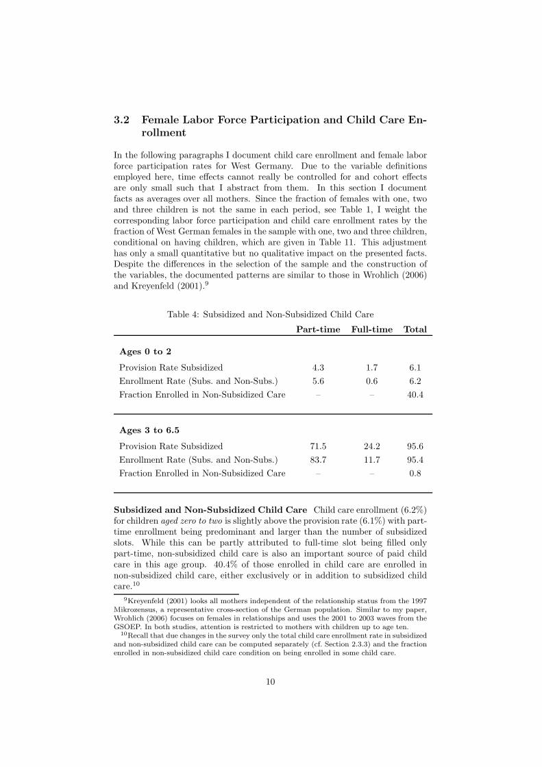
Table 4: Subsidized and Non-Subsidized Child Care

Part-time Full-time Total

Ages 0 to 2

Provision Rate Subsidized 4.3 1.7 6.1

Enrollment Rate (Subs. and Non-Subs.) 5.6 0.6 6.2

Fraction Enrolled in Non-Subsidized Care – – 40.4

Ages 3 to 6.5

Provision Rate Subsidized 71.5 24.2 95.6

Enrollment Rate (Subs. and Non-Subs.) 83.7 11.7 95.4

Fraction Enrolled in Non-Subsidized Care – – 0.8

Subsidized and Non-Subsidized Child Care Child care enrollment (6.2%)for children aged zero to two is slightly above the provision rate (6.1%) with part-time enrollment being predominant and larger than the number of subsidizedslots. While this can be partly attributed to full-time slot being filled onlypart-time, non-subsidized child care is also an important source of paid childcare in this age group. 40.4% of those enrolled in child care are enrolled innon-subsidized child care, either exclusively or in addition to subsidized childcare.10

9Kreyenfeld (2001) looks all mothers independent of the relationship status from the 1997Mikrozensus, a representative cross-section of the German population. Similar to my paper,Wrohlich (2006) focuses on females in relationships and uses the 2001 to 2003 waves from theGSOEP. In both studies, attention is restricted to mothers with children up to age ten.

10Recall that due changes in the survey only the total child care enrollment rate in subsidizedand non-subsidized child care can be computed separately (cf. Section 2.3.3) and the fractionenrolled in non-subsidized child care condition on being enrolled in some child care.

10

The picture looks entirely different for children aged three to six and a half.

Enrollment increases to over 95.4% and matches up very closely with the pro-vision rate. Part-time child care is used much more than full-time care andagain exceeds the supply of part-time slots. However, for this age group this isexplained by the number of full-time slots being filled part-time as opposed tonon-subsidized child care, which is negligible in absolute and relative terms.

Table 5: Child Care Enrollment RateConditional on Maternal Labor Force Participation Status

Ages0 to 2 3 to 6.5

At least part-time care

Not Working 2.9 93.2

Part-time Working 11.8 96.6

Full-time Working 24.4 97.0

Full-time care

Full-time Working 3.9 32.4

Child Care Enrollment by Maternal Labor Force Participation Table5 shows the overall child care enrollment rate conditional on the maternal laborforce participation status (upper panel) and the full-time child care enrollmentrate of full-time working mothers (lower panel). This table highlights two ofthe facts discussed in the introduction for the cross-section of OECD countries.While children are of ages zero to two, only 11.8% of the part-time and 24.4%of the full-time working mothers use some paid child care, and for the lattergroup only 3.9% use full-time care. The remainder of working females, i.e. thevast majority, is not using any paid child care. Given the age of the childrenand since virtually all husbands are working full-time, these females necessarilyuse some form of non-paid child care, e.g. own parents (in law) or other familymembers and friends, to free up the time to work. In contrast, for children agedthree to six and a half the enrollment rate is nearly independent of the maternallabor force participation status, even 93.2% of the non-working females use childcare. However, with regard to full-time working females again only 32.4% usepaid full-time child care and thus 67.6% use at least some non-paid child care.

Labor Supply and Child Care While the facts presented in the previousparagraph show the relative numbers of females not using child care and work-ing and the relative numbers of females using child care but not working, thequantitative importance of these groups becomes obvious only when looking atthe female participation rates. More than 30% of the females with a child of ageszero to two are working and still close to 40% of the females with a child of agesthree to six and half are not working, cf. the left panel of Figure 4. Attempts

11

Figure 4: Labor Force Participation and Child Care Enrollment Rates0

1020

3040

5060

7080

9010

0%

<3 <6.5 <9.5 <12.5 <15.5 <18.5Age youngest child

Participation Rate

Enrollment Rate

Total

010

2030

4050

6070

8090

100

%<3 <6.5 <9.5 <12.5 <15.5 <18.5

Age youngest child

Participation Rate: Part−time Full−time

Enrollment Rate: Part−time Full−time

Part− vs. Full−time

to quantify the role of child care for female labor force participation need toacknowledge the fact that a large fraction of females works without using paidchild care but also uses paid child care without working.

The maternal labor force participation rate increases the strongest in the earlyperiods of a child’s life but levels off later in life at 80%. The right panel of Figure4 provides the split of the overall participation and enrollment rates by part-and full-time. As for the enrollment rates, cf. Table 4, part-time participationdominates and explains the shape of the overall participation rate whereas full-time participation increases nearly linearly from 5% to 20% throughout a child’sadolescence.

3.3 Summary Key Facts

The facts documented in this Section about labor force participation of marriedfemales with children and their child care enrollment decisions can be summa-rized as follows:

1. Subsidized child care is on the one hand around four times as cheap asnon-subsidized child care, but on the other hand only provided for veryfew children aged zero to two whereas for nearly all children aged three tosix and half.

2. Enrollment rates in child care match up with the provision rates whilenon-subsidized child care is only important for children aged zero to two.

12

3. Child care is on the one hand used by non-working females but on theother hand not used be working females.

4. The labor force participation rate grows strongly while children are ofpre-school age and less afterwards.

In the next Section, I develop a life-cycle model that aims to capture this set ofstylized facts for West Germany.

4 The Model

The model is based on the setup by Greenwood et al. (2003). While I abstractfrom marriage and divorce decisions and the implied equilibrium considerationsdiscussed in their work, I extend the model by child care and a richer life-cyclestructure.

4.1 Demographics

A female lives for six periods and is exogenously matched with a man at thebeginning of her life. By then she chooses how many children to have and boththe husband and children stay with her throughout her whole life. In case thefemale chooses to have more all children are born as multiples. This simplifyingassumption is guided by one of the two objectives of the analysis: to quantifythe importance of child care on the total number of children a female desiresto have. The period length corresponds to three years reflecting the distinctivestages of a child’s adolescence, compare Figure 3.11

4.2 Endowments

Each female and her husband are indexed by productivity levels ǫ and ǫ∗ rep-resenting the stochastic part of each spouses’ market wages (Asterisks refer toparameters for the husband. Both spouses are assigned initial productivity lev-els (ǫ, ǫ∗) in period one which follow an AR(1) process over time:

ǫt = ρǫt−1 + εt with εt ∼ N(0, σ2ε)

ǫ∗t = ρ∗ǫ∗t−1 + ε∗t with ε∗t ∼ N(0, σ2ε∗)

(1)

In the first two periods while the children are not yet in school, females canenroll them in subsidized and/or non-subsidized child care. Both types of childcare are perfect substitutes with the exception of the price and availability. Incontrast to non-subsidized child care, I assume that access to subsidized childcare slots, denoted as at, is rationed and randomly assigned to mothers by alottery with time-dependent success probabilities.

11For period two the overlap is not exact since the mean duration in the data is three anda half years.

13

4.3 Preferences

The female is assumed to be the household’s sole decision maker and her per-period utility function consists of four additive parts reflecting the utility fromher share of consumption, her leisure, the number of children and a measure ofchild quality:12

ut =(ψ(n)ct)

1−γ0 − 1

1 − γ0+ δ1

(1 − lt −mt)1−γ1 − 1

1 − γ1+ δ2

(1 + n)1−γ2 − 1

1 − γ2+ Qt.

(2)

4.3.1 Consumption

Household consumption ct is transformed into the consumption realized by anadult, the female’s share, using the OECD equivalence scale (Oxford scale):

ψ(n) =1

1.7 + 0.5n, (3)

with n being the number of children in the household. The budget constraintis given by:

ct = τ [yt(lt, xt, ǫt), y∗t (t, ǫ∗t )] − pcc [n, t, ccs,t, ccns,t, yt, y

∗t ] + T [n, t, lt] . (4)

The function τ calculates the after tax household income from the female’s (yt)and husband’s (y∗t ) gross income. The latter depends on two components: adeterministic component in time t (in line with the all husbands are assumedto work full-time and thus accumulate full-time experience) and a stochasticcomponent represented by the husband’s current period productivity shock (ǫ∗).In contrast, the female’s income depends on her labor supply (lt), accumulatedexperience through past labor force participation

xt = xt−1 + lt−1, (5)

and her current period productivity shock (ǫft ).

Child care fees pcc are related to the number of (n) and age (t) of the children,the utilized amount of subsidized (ccs,t) and non-subsidized (ccns,t) child careas well as the gross household income.

In addition, households receive transfers T conditional on the time period (t)and choices (n, lt).

The functional forms for the gross incomes y and y∗, the tax schedule τ , thechild care pricing function pcc and transfers T are specified further below inSection 5.1.

4.3.2 Leisure

Each female is endowed with one unit of non-sleeping time which is reduced bylabor force supply (lt), and maternal time investment (mt) in her children.

12Greenwood et al. (2003) interact the utility from having children with child quality. Sim-ilar to one of the specifications in Jones et al. (2008) I use separability which allows me to pindown the parameters by moments more clearly.

14

4.3.3 Children

Children enter the utility function directly in form of a durable consumptiongood.

4.3.4 Child quality

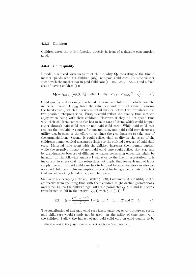
I model a reduced form measure of child quality Qt consisting of the time amother spends with her children (mt), non-paid child care, i.e. time neitherspend with the mother nor in paid child care (1−mt− ccs,t − ccns,t) and a fixedcost of having children (ζ):

Qt = I{n>0}

(

δ3ξ(t)mγ3 − φ(t) (1 −mt − ccs,t − ccns,t)

φ3 − ζ)

. (6)

Child quality matters only if a female has indeed children in which case theindicator function I{n>0} takes the value one and zero otherwise. Ignoringthe fixed costs ζ which I discuss in detail further below, this formulation hastwo possible interpretations. First, it could reflect the quality time mothersenjoy when being with their children. However, if they do not spend timewith their children, someone else has to take care of them, which could happeneither through paid child care or non-paid child care. While paid child carereduces the available resources for consumption, non-paid child care decreasesutility, e.g. because of the effort to convince the grandparents to take care ofthe grandchildren. Second, it could reflect child quality in the sense of thechildren’s human capital measured relative to the omitted category of paid childcare. Maternal time spent with the children increases their human capital,while the negative impact of non-paid child care could reflect that e.g. careby grandparents because of different attitudes concerning education might beharmful. In the following analysis I will stick to the first interpretation. It isimportant to stress that this setup does not imply that for each unit of laborsupply one unit of paid child care has to be used because females can also usenon-paid child care. This assumption is crucial for being able to match the factthat not all working females use paid child care.

Similar to the setup by Hotz and Miller (1988), I assume that the utility moth-ers receive from spending time with their children might decline geometricallyover time, i.e. as the children age, with the parameter ξ1 > 0 and is linearlytransformed to fall in the interval [ξ2, 1] with ξ2 ∈ [0, 1]:13

ξ(t) = ξ2 +t−ξ1 − T−ξ1

1 − T−ξ1

(1 − ξ2) for t = 1, . . . , T and T = 6. (7)

The contribution of non-paid child care has to enter negatively, otherwise costlypaid child care would simply not be used. As the utility of time spent withthe children, I allow the impact of non-paid child care on child quality to be

13In Hotz and Miller (1988), this is not a choice but a fixed time cost.

15

age-dependent, i.e.

φ(t) =

φ1 for t = 1φ2 for t = 20 for t > 2

= φI{t=1}

1 φI{t=2}

2 I{t≤2},

(8)

where I{cond} is the indicator function that takes the value of one when cond istrue and zero otherwise. With the focus of the analysis in this paper lying onpre-school child care I do not model child care once children enter school andas a consequence do not consider the impact of non-paid child care anymore. Iassume that every female can use as much non-paid child care as she desires.It might be argued that some females have access to non-paid child care andothers not, e.g. because some live closer and other further away from the ownparents or parents in law who are the most likely provider of non-paid child care.This information is available for three years (1991, 1996, 2001) in the GSOEPfor five categories: living in same house, same neighborhood, same city, within1h driving distance, further away/non-existent. Surprisingly, the participationrates for females with children aged zero to two, and aged three to six and ahalf, are essentially independent from this distance measure, see Table 20 inAppendix B. Although this is no evidence in favor of homogenous access to orcosts of non-paid child care, it is at least not a rejection of this assumption.

Finally, the parameter ζ is deducted from the child quality measure for a techni-cal reason. Since ζ is fixed, conditional on having children ζ neither affects thechoice of maternal time investment nor of child care usage but only the n = 0vs. n > 0 decision. The negative fixed cost of having children counteracts thelarge utility increase females experience from having the first child through thebenefit of spending time with the children (although the net effect might belower in periods one and two if non-paid child care is used) and the fact thatthe difference in the utility derived from the pure presence of children (δ2, γ2)is the largest for the n = 0 vs. n = 1. In economic terms ζ essentially rescalesthe utility from spending time with children.

4.4 Choice Variables

All choices are assumed to be discrete. Labor supply l can take on three values:

lt =

0 for non-working14 for part-time work12 for full-time work

∀ t = 1, . . . , 6. (9)

If the (non-sleeping) time endowment would be 16 hours, then part-time workwould correspond to four and full-time work to eight hours. Similarly, subsidizedccs and non-subsidized child care ccns can take on three values:

cci,t =

0 for no paid child care14 for part-time paid child care12 for full-time paid child care

∀ t = 1, 2 and i = s, ns. (10)

16

The actual choice for subsidized is child care is however restricted by the accessat to a subsidized child care slot:

at =

0 no access to subsidized child care14 access to a part-time subsidized child care slots12 access to a part-time subsidized child care slots

∀ t = 1, 2 (11)

such thatccs,t ≤ at ∀ t = 1, 2. (12)

Access to a subsidized child care slot is determined by a lottery with age- andtype-dependent, i.e. part- or full-time, success probabilities. Paid child care insubsidized and non-subsidized arrangements is restricted to to

ccs,t + ccns,t ≤1

2∀ t = 1, 2, (13)

which could be interpreted such that child care facilities are only open duringthe first half of the day, i.e. in the morning and early afternoon. A mother canstill spend time with her children in the late afternoon and evening such thatin principle

mt ∈ {0,1

4,1

2,3

4, 1}. (14)

However, a mother cannot spend time with her children while these are in childcare or she is working. Once children are of school age, ccs,t is replaced by thetime spend in mandatory, costless school st:

mt ≤

{1 − max{lt, ccs,t + ccns,t} ∀ t ≤ 21 − max{lt, st} ∀ 3 ≤ t ≤ 6

. (15)

4.5 Dynamic Problem

Figure 5 presents the timing of events during a female’s life which is definedby the stages of her children’s adolescence, compare also Figure 3. The termzt combines the productivity states of both spouses (ǫt, ǫ

∗t ) and the female’s

experience level (xt, with x1 = 0). The first period is split up in two stages withdifferent state and decision variables. In the first stage, the initial productivitylevels are assigned and the female chooses the optimal number of children (n)taking into account the uncertainty with respect to the access to subsidizedchild care:

maxn

{Ea1V (1, ǫ1, ǫ

∗1, x1, n, a1), n = 0, 1, 2, ..., N} . (16)

Once the optimal number of children (n) is chosen, n becomes a state variablesince the children stay with the mother throughout her entire life. After accessto subsidized child care is determined by a lottery, the female decides on herlabor supply (l1) and those with children, on how much time to spend with them(m1) and on their enrollment in subsidized child care (ccs,1) – possibly restricted(by a1) – and non-subsidized child care (ccns,1). The following Bellman equationrepresents the female’s problem in the second stage:

V (1, ǫ1, ǫ∗1, x1, n, a1) = max

m,l,ccs≤a1,ccns

ut + βEǫ,ǫ∗,a2V (2, ǫ2, ǫ

∗2, x2, n, a2)

subject to (4), (5), (13) and (15).(17)

17

Figure 5: Life Cycle

States

Choices

† zt = {ǫt, ǫ∗t, xt}

Pre-school School

1

z1†

n

z1, n,

a1

l,m

cc,

2

z2, n,

a2

l,m

cc,

3

z3, n

l,m

4

z4, n

l,m

5

z5, n

l,m

6

z6, n

l,m

ut is given by Equation (2) and β is the discount factor. At the beginning ofperiod two, the new productivity levels (ǫt, ǫ

∗t ) realize according to the AR(1)

process specified in Equation (1) and access to child care (a2) is drawn from anew lottery. The set of choice variables in period two is identical to the seconddecision stage in period one. The value function in period two is

V (2, ǫ2, ǫ∗2, x2, n, a2) = max

m,l,ccs≤a2,ccns

ut + βEǫ,ǫ∗V (3, ǫ3, ǫ∗3, x3, n, 0)

subject to (4), (5), (13) and (15).(18)

From period three onwards, children attend school and females cannot use childcare anymore (at = 0 for t ≥ 3). Subsequently, a female only decides on howmuch to work and how much time to spend with their children:

V (t, ǫt, ǫ∗t , xt, n, 0) =max

m,lut + βEǫ,ǫ∗V (t+ 1, ǫt+1, ǫ

∗t+1, xt+1, n, 0) ∀ 3 ≤ t ≤ 5

subject to (4), (5) and (15).

(19)

In the last period, the female only maximizes the current-period utility:

V (6, ǫ6, ǫ∗6, x6, n, 0) = max

m,lut subject to (4) and (15). (20)

4.6 Maternal Leave

An important element affecting labor force participation decisions of femaleswith children aged zero to two is the German maternal leave regulation. Itpermits every mother who has been working until the birth of a child to returnto her pre-birth employer at her pre-birth wage within three years after birth.Since in the model life starts with the birth decision, there is no pre-birth laborsupply and I therefore grant all females the right to go on maternal leave.14

By construction, part- and full-time working mothers work at their “pre-birth”

14In the sample investigated here, 94% of all mothers work prior to the first birth.

18

wage in period one. Hence, the maternal leave regulation has only to be mod-eled explicitly for mothers that do not work in the first period, i.e. for whichl1 = 0 or equivalently x2 = 0. I assume that their offered wage in the secondperiod is given by y2 (l2, 0,max{ǫ1, ǫ2}) and the third period productivity levelis determined by

ǫ3 =

{ρ max{ǫ1, ǫ2} + ε3 if l1 = 0, l2 > 0ρǫ2 + ε3 else.

5 Calibration

Before turning to the calibration of the preference parameters and discussingthe corresponding data moments, I present the functional forms for the so farunspecified elements of the budget constraint.

5.1 Elements of the budget constraint

5.1.1 Income

Husbands In line with the data, all husbands are assumed to be working full-time. I assume that the log of their gross income Y ∗

t is a concave function oftime (in the model) or, respectively, of the youngest child’s age (in the data):

ln Y ∗t = η∗0 + η∗1(t− 1) + η∗2(t− 1)2 + ǫ∗t , (21)

with y∗t = eY ∗t . Equation (21) as well as the persistence parameter ρ∗ of the

income shock ǫ∗t (Equation (1)) can be estimated directly from the data. Theperiod income is defined as the total labor income, including side jobs andself-employment, pensions, unemployment benefits (to capture the full risk ofthe income process), compensation for further training or education, and anyadditional payments as 13th and 14th salary, vacation and Christmas pay or anyfurther boni received during the period.

Females The gross full-time income Yt of a female is given by a classical Mincer(1974) earnings equation with returns to experience. As a normalization xt ismultiplied by two (xt = 2xt) such that part-time work increases x by 0.5 andfull-time work by 1:

ln Yt = η0 + η1xt + η2x2t + ǫt, (22)

with y(lt = 1, xt, ǫt) = 12e

Yt for part-time and y(lt = 2, xt, ǫt) = eYt for full-timeworking females.

While for the husbands the wage equations (21) and (1) can be estimated di-rectly, this is more difficult for females since a consistent mapping between themeasure of experience in the model and experience in the data is only feasiblefor females observed prior to their first birth. I therefore assume that femalesface the same wage process as their husbands but take into account that they areon average 2.9 years younger and introduce a gender gap in wages originatingfrom gender differences in education and occupational choices and potentially adiscriminatory component.

19

The age difference of nearly three years corresponds to one model period. I shiftthe income process for husbands by one period to obtain that of females, as afemale that has worked full-time in all periods, i.e. xt = t − 1, should receivethe same (deterministic) wage a male had in the period before because of theage difference

ln Yt(xt = t− 1) = lnY ∗t−1

= η∗0 + η∗1(t− 1︸ ︷︷ ︸

xt

− 1) + η∗2(t− 1︸ ︷︷ ︸

xt

− 1)2 + ǫt (23)

Equation (23) can then be reformulated to obtain the coefficients of the femaleincome process:

ln Yt =η∗0 − η∗1 + η∗2︸ ︷︷ ︸

η0

+ [η∗1 − 2η∗2 ]︸ ︷︷ ︸

η1

xt + η∗2︸︷︷︸

η2

x2t + ǫt

(24)

This implies that in the model in a given period, where husbands and femalesby construction have the same age, females have a lower mean wage and facelarger returns to experience than their spouses if η∗2 < 0. Using the full-timewages of both sexes prior to the first birth, the gender wage gap in mean incomenot driven by the age difference can be estimated and added to the log of thegross income:15

η0 = η∗0 − η∗1 + η∗2 + ∆gender . (25)

The last missing piece of the income process concerns the stochastic part (Equa-tion (1)) where I follow Attanasio et al. (2008) and use the male estimates forthe females.

Table 6 and Figure 6 summarize the estimation results on the income process.It is worthwhile to mention that the difference between η0 and η∗0 without thegender wage gap is -0.058. Not controlling for age would increase the pre-birthgender wage gap by -0.069. Thus, using the same experience profile for husbandsand females but shifting it by one period as done in Equation (23) and Equation(24) provides an accurate estimate of the pre-birth gender income difference dueto the age difference of spouses.

For the numerical solution of the model, the AR(1) process for the productiv-ity shock (Equation (1)) is discretized using the method proposed by Tauchen(1986) into 20 states. The initial productivity levels are assigned according tothe corresponding stationary distribution.

5.1.2 Tax Code

The tax code implemented in the model incorporates the three key elements ofthe German tax system: progressive and joint taxation, and mandatory socialsecurity contributions.

Progressivity The tax code is based on the average income taxes over thesample period in 2008 e, which are available (in nominal terms) for each

15By then 75% of the females are working full-time such that selection into full-time em-ployment is less of a problem.

20

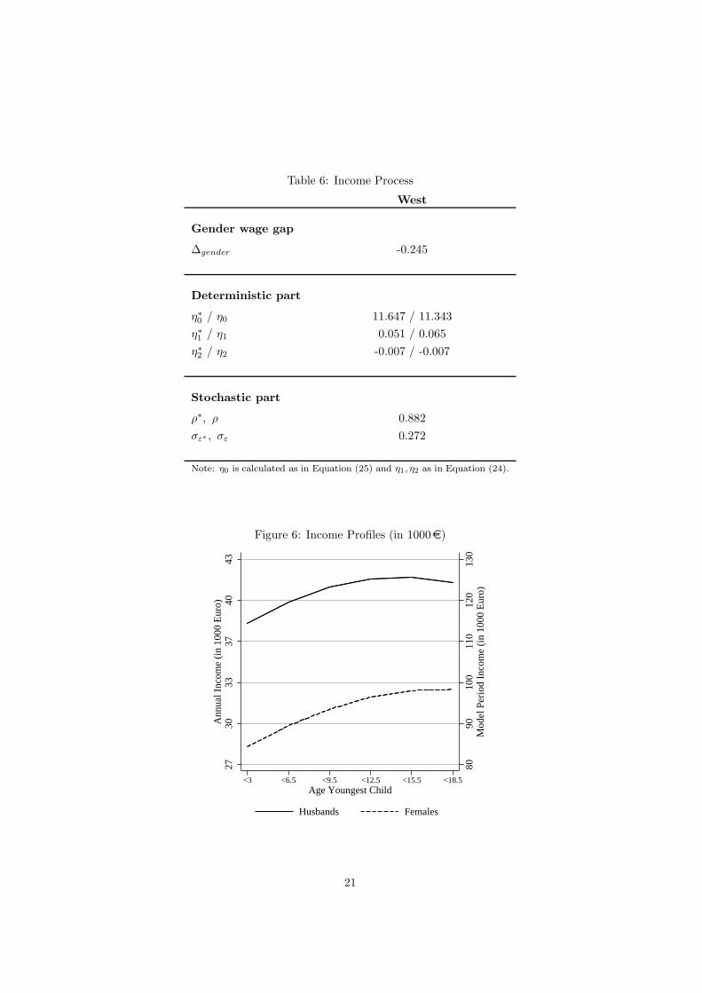
Table 6: Income Process

West

Gender wage gap

∆gender -0.245

Deterministic part

η∗0 / η0 11.647 / 11.343

η∗1 / η1 0.051 / 0.065

η∗2 / η2 -0.007 / -0.007

Stochastic part

ρ∗, ρ 0.882

σε∗ , σε 0.272

Note: η0 is calculated as in Equation (25) and η1, η2 as in Equation (24).

Figure 6: Income Profiles (in 1000e)

8090

100

110

120

130

Mod

el P

erio

d In

com

e (in

100

0 E

uro)

2730

3337

4043

Ann

ual I

ncom

e (in

100

0 E

uro)

<3 <6.5 <9.5 <12.5 <15.5 <18.5Age Youngest Child

Husbands Females

21

year on the website of the German Federal Ministry of Finance(https://www.abgabenrechner.de/). The tax code consists of three parts sep-arated by two thresholds. First, annual income up to 3282e, the smallest incometax allowance in the years 1983 to 2006 is tax-exempted. Second, every e above100,000e is taxed linearly at a marginal rate of 52%. Third, every e betweenthe two thresholds is taxed at an increasing marginal rate. The coefficients forthis part are obtained by regressing the average tax burden over the sampleperiod on a seventh order polynomial of taxable income, i.e. income less the taxallowance, associated with a R2 of 1.00. The upper threshold of 100,000e waschosen because for higher incomes the average marginal taxes does not changeanymore. Figure 7 and Table 7 summarize the information on the progressivityof the tax code implemented in this paper on and annual basis and for the modelperiod of three year length.

Table 7: Annual Taxes

Frequency Taxable Income (y) Tax Burden

Annual 0 - 3282 0

Model Period 0 - 9846 0

Annual 3283 - 100000∑7

i=1 βi(y − 3282)i

Model Period 9847 - 100000∑7

i=1 βi(y − 9846)i

β1=.07415027β2=.00001249β3=-3.990e-10β4=9.011e-15β5=-1.143e-19β6=7.456e-25β7=-1.964e-30

Annual 100001 - ∞∑7

i=1 βi(1e5 − 3282)i+(y-1e5)×0.52

Model Period 300001 - ∞∑7

i=1 βi(3e5 − 9846)i+(y-3e5)×0.52

Source: German Federal Ministry of Finance, own calculations. Figures are averages over theyears 1983 to 2006 expressed in 2008 e.

Joint Taxation Married couples are taxed jointly. The sum of the spouses’incomes is divided by two, the tax burden is calculated according to the tax codeand doubled afterwards. Because of the progressivity of the tax system, thejoint net income is larger compared to individual taxation as long as one spouseearns more than the other and at least one income remains below 100,000e.Joint taxation is only feasible for legally married partners. Although my samplecontains cohabitating but not legally married partners I apply joint taxation forall couples.

22

Figure 7: Annual Taxes and Tax Rates0

1020

3040

5060

7080

9010

011

0T

ax B

urde

n/A

fter

Tax

Inco

me

(in 1

000

Eur

o)

0 10 20 30 40 50 60 70 80 90 100 110Before−Tax Income (in 1000 Euro)

After−Tax Income Tax Burden

05

1015

2025

3035

4045

5055

Per

cent

age

Poi

nts

0 10 20 30 40 50 60 70 80 90 100 110Before−Tax Income (in 1000 Euro)

Marginal Tax Rate Average Tax Rate

Source: German Federal Ministry of Finance, own calculations. Figures are averages over theyears 1983 to 2006 expressed in 2008 e.

Mandatory social security contributions Employees, excluding civil ser-vants, have to make mandatory contributions to the pension system, unemploy-ment, long-term care and public health insurance which accrue proportionallyup to certain income threshold. Any income above the threshold is not subjectto the contribution anymore. Table 8 shows the average monthly and model pe-riod thresholds and contribution rates for each type of insurance over the years1983 to 2006 in 2008e.

Table 8: Social Security Contributions

Insurance Contribution Contribution LimitType Rate (%) Monthly Model Period

Unemployment 3.46 4849.86 174594.81

Pensions 10.28 4849.86 174594.81

Health 7.27 3557.66 128075.93

Long Term Care 0.41 3557.66 128075.93

Source: German Federal Ministry of Labor and Social Affairs. Figures areaverages over the years 1983 to 2006 expressed in 2008 e and represent theemployee’s contributions.

Implementation The income tax and mandatory social security contributionsrefer to annual and monthly values whereas the model periods correspond tothree years. I therefore divide the incomes in the model by three to obtainannual values, calculate after-tax income under using the tax code defined above

23

under joint taxation, deduct annual social security contributions and multiplythe resulting value by three to return to the three year period values.

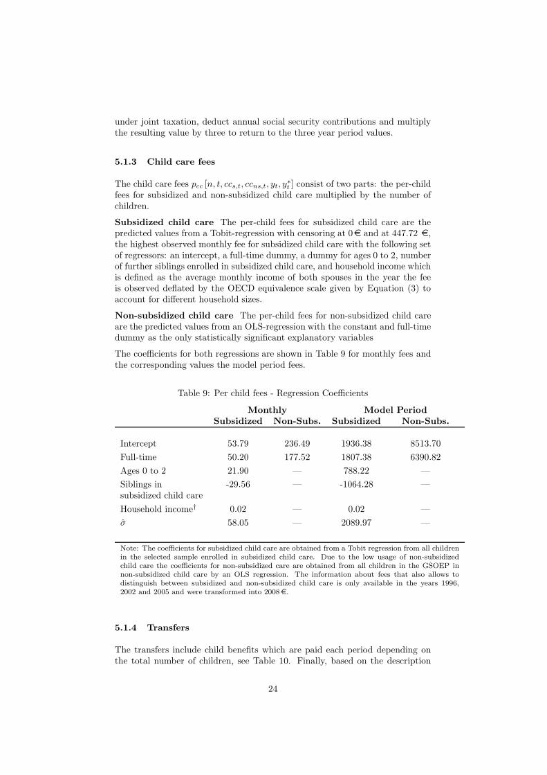
5.1.3 Child care fees

The child care fees pcc [n, t, ccs,t, ccns,t, yt, y∗t ] consist of two parts: the per-child

fees for subsidized and non-subsidized child care multiplied by the number ofchildren.

Subsidized child care The per-child fees for subsidized child care are thepredicted values from a Tobit-regression with censoring at 0e and at 447.72 e,the highest observed monthly fee for subsidized child care with the following setof regressors: an intercept, a full-time dummy, a dummy for ages 0 to 2, numberof further siblings enrolled in subsidized child care, and household income whichis defined as the average monthly income of both spouses in the year the feeis observed deflated by the OECD equivalence scale given by Equation (3) toaccount for different household sizes.

Non-subsidized child care The per-child fees for non-subsidized child careare the predicted values from an OLS-regression with the constant and full-timedummy as the only statistically significant explanatory variables

The coefficients for both regressions are shown in Table 9 for monthly fees andthe corresponding values the model period fees.

Table 9: Per child fees - Regression Coefficients

Monthly Model PeriodSubsidized Non-Subs. Subsidized Non-Subs.

Intercept 53.79 236.49 1936.38 8513.70

Full-time 50.20 177.52 1807.38 6390.82

Ages 0 to 2 21.90 — 788.22 —

Siblings in -29.56 — -1064.28 —subsidized child care

Household income† 0.02 — 0.02 —

σ 58.05 — 2089.97 —

Note: The coefficients for subsidized child care are obtained from a Tobit regression from all childrenin the selected sample enrolled in subsidized child care. Due to the low usage of non-subsidizedchild care the coefficients for non-subsidized care are obtained from all children in the GSOEP innon-subsidized child care by an OLS regression. The information about fees that also allows todistinguish between subsidized and non-subsidized child care is only available in the years 1996,2002 and 2005 and were transformed into 2008e.

5.1.4 Transfers

The transfers include child benefits which are paid each period depending onthe total number of children, see Table 10. Finally, based on the description

24

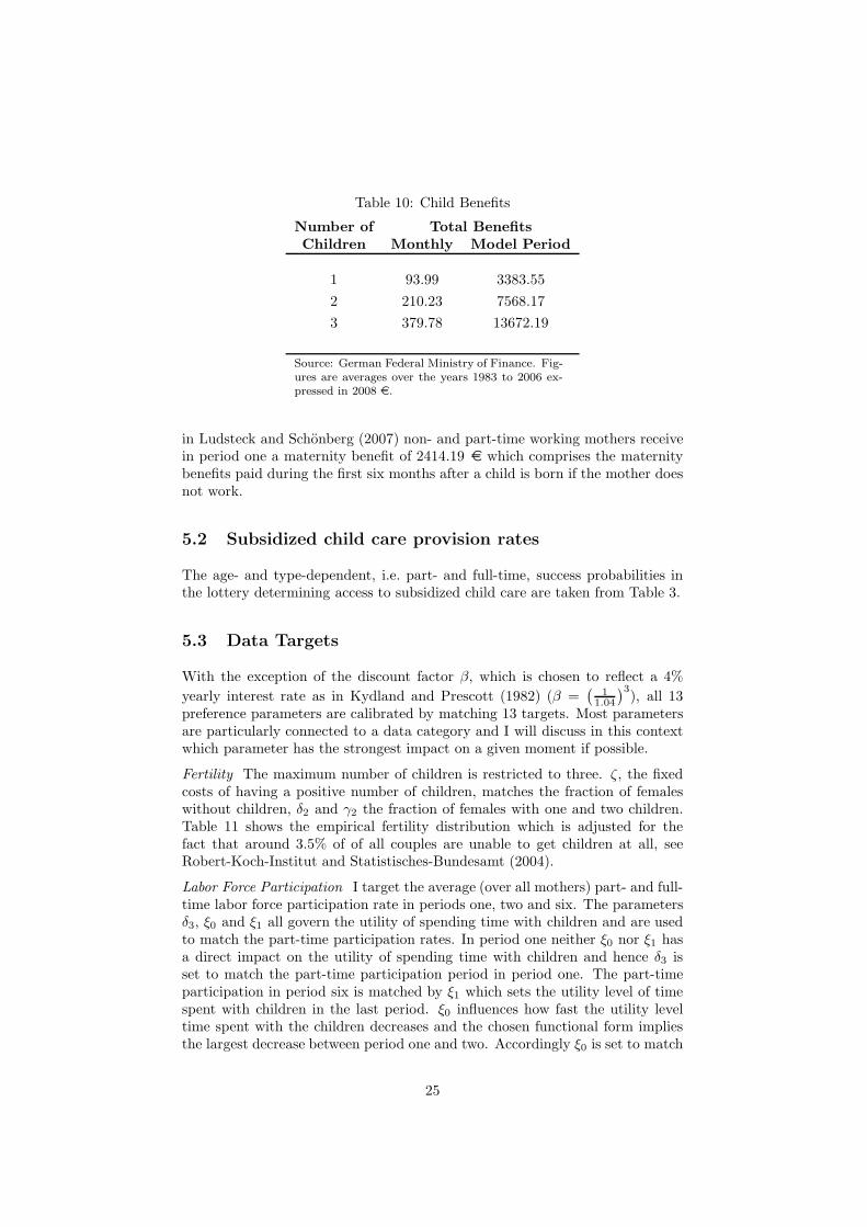
Table 10: Child Benefits

Number of Total BenefitsChildren Monthly Model Period

1 93.99 3383.55

2 210.23 7568.17

3 379.78 13672.19

Source: German Federal Ministry of Finance. Fig-ures are averages over the years 1983 to 2006 ex-pressed in 2008 e.

in Ludsteck and Schonberg (2007) non- and part-time working mothers receivein period one a maternity benefit of 2414.19 e which comprises the maternitybenefits paid during the first six months after a child is born if the mother doesnot work.

5.2 Subsidized child care provision rates

The age- and type-dependent, i.e. part- and full-time, success probabilities inthe lottery determining access to subsidized child care are taken from Table 3.

5.3 Data Targets

With the exception of the discount factor β, which is chosen to reflect a 4%

yearly interest rate as in Kydland and Prescott (1982) (β =(

11.04

)3), all 13

preference parameters are calibrated by matching 13 targets. Most parametersare particularly connected to a data category and I will discuss in this contextwhich parameter has the strongest impact on a given moment if possible.

Fertility The maximum number of children is restricted to three. ζ, the fixedcosts of having a positive number of children, matches the fraction of femaleswithout children, δ2 and γ2 the fraction of females with one and two children.Table 11 shows the empirical fertility distribution which is adjusted for thefact that around 3.5% of of all couples are unable to get children at all, seeRobert-Koch-Institut and Statistisches-Bundesamt (2004).

Labor Force Participation I target the average (over all mothers) part- and full-time labor force participation rate in periods one, two and six. The parametersδ3, ξ0 and ξ1 all govern the utility of spending time with children and are usedto match the part-time participation rates. In period one neither ξ0 nor ξ1 hasa direct impact on the utility of spending time with children and hence δ3 isset to match the part-time participation period in period one. The part-timeparticipation in period six is matched by ξ1 which sets the utility level of timespent with children in the last period. ξ0 influences how fast the utility leveltime spent with the children decreases and the chosen functional form impliesthe largest decrease between period one and two. Accordingly ξ0 is set to match

25

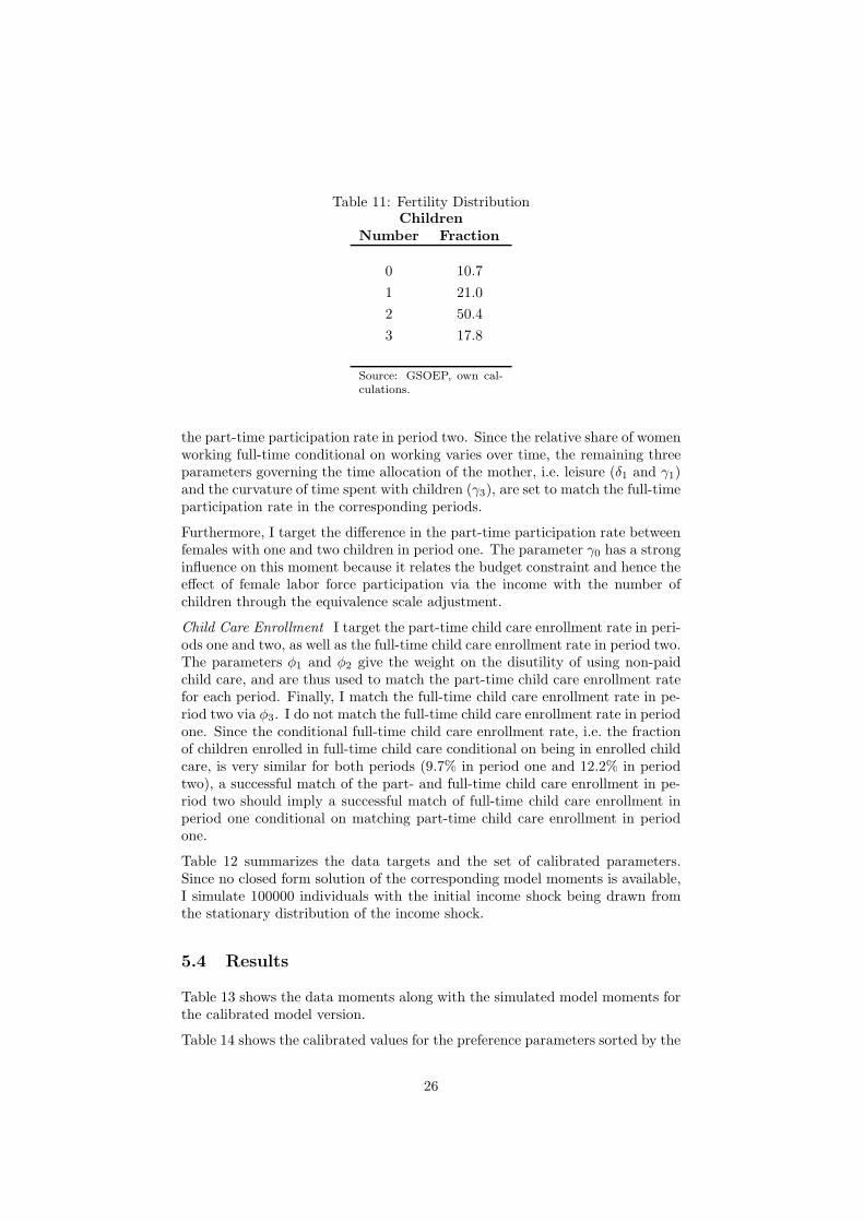
Table 11: Fertility DistributionChildren

Number Fraction

0 10.7

1 21.0

2 50.4

3 17.8

Source: GSOEP, own cal-culations.

the part-time participation rate in period two. Since the relative share of womenworking full-time conditional on working varies over time, the remaining threeparameters governing the time allocation of the mother, i.e. leisure (δ1 and γ1)and the curvature of time spent with children (γ3), are set to match the full-timeparticipation rate in the corresponding periods.

Furthermore, I target the difference in the part-time participation rate betweenfemales with one and two children in period one. The parameter γ0 has a stronginfluence on this moment because it relates the budget constraint and hence theeffect of female labor force participation via the income with the number ofchildren through the equivalence scale adjustment.

Child Care Enrollment I target the part-time child care enrollment rate in peri-ods one and two, as well as the full-time child care enrollment rate in period two.The parameters φ1 and φ2 give the weight on the disutility of using non-paidchild care, and are thus used to match the part-time child care enrollment ratefor each period. Finally, I match the full-time child care enrollment rate in pe-riod two via φ3. I do not match the full-time child care enrollment rate in periodone. Since the conditional full-time child care enrollment rate, i.e. the fractionof children enrolled in full-time child care conditional on being in enrolled childcare, is very similar for both periods (9.7% in period one and 12.2% in periodtwo), a successful match of the part- and full-time child care enrollment in pe-riod two should imply a successful match of full-time child care enrollment inperiod one conditional on matching part-time child care enrollment in periodone.

Table 12 summarizes the data targets and the set of calibrated parameters.Since no closed form solution of the corresponding model moments is available,I simulate 100000 individuals with the initial income shock being drawn fromthe stationary distribution of the income shock.

5.4 Results

Table 13 shows the data moments along with the simulated model moments forthe calibrated model version.

Table 14 shows the calibrated values for the preference parameters sorted by the

26

Table 12: Data targets and parametersTarget Parameter

Fertility

Fraction of femaleswithout children ζ

with one and two children δ2, γ2

Labor Force Participation Rate

Part-timet = 1 δ3t = 2 ξ0t = 6 ξ1t = 1; ∆{n=1}−{n=2} γ0

Full-timet = 1, 2, 6 δ1, γ1, γ3

Child Care Enrollment Rate

Part-timet = 1 φ1

t = 2 φ2

Full-timet = 2 φ3

Note: Labor force participation and child care enrollmentrates are averages over all mothers.

27

Table 13: Targeted data and model momentsTarget Data Model Difference

Fertility

Fraction of femaleswith out children 10.7 10.1 0.6with one child 21.0 20.0 1.1with two children 50.4 51.2 -0.8

Labor Force Participation Rate

Part-timet = 1 26.5 26.2 0.3t = 2 53.2 53.6 -0.4t = 6 60.0 56.8 3.1t = 1; ∆{n=1}−{n=2} 10.9 11.5 -0.6

Full-timet = 1 4.7 5.1 -0.5t = 2 8.4 8.7 -0.3t = 6 19.7 16.5 3.1

Child Care Enrollment Rate

Part-timet = 1 5.6 5.1 0.5t = 2 83.7 81.8 1.8

Full-timet = 2 11.6 12.9 -1.3

28

calibration targets and with reference to the corresponding part in the utilityfunction. While not all parameters, in particular the utility weights δi i = 1, 2, 3,

Table 14: Preference parameters

Fertility

Number of children δ2= 1.13 γ2= 1.39

Fixed cost of children ζ= 0.60

Labor Force Participation

Consumption γ0= 2.00

Leisure δ1= 0.35 γ1= 1.92

Maternal time δ3= 2.20 γ3= 0.46 ξ0= 0.03 ξ1= 0.46

Child Care Enrollment

Non-paid child care φ1= 0.49 φ2= 0.45 φ3= 2.40

do not have a concrete interpretation, a few comments can be made. First, asalready discussed the fixed costs of having children ζ = 0.6 rescale the level ofutility from spending time with children which only affects the decision of havingvs. not having children. The parameter values for the utility from spending timetime with children and ζ imply that for a female spending at least one unit oftime (mt = 1

4 ) with her children Qt is always positive, with the exception ofthe last period (Q6 = −0.06), even if in the first two periods no paid childcare at all is used. Second, the curvature of consumption γ0 = 2.00 is in therange of usually cited values. The utility of maternal time in the last period is(ξ0 = 0.46) slightly less than half of the value in the first period and decreasesat a very modest speed over rate (ξ1 = 0.03). Finally, using non-paid child carefor children aged three to six and a half is associated with a lower utility costthan for children aged zero to two (φ2 = 0.45 vs. φ1 = 0.49).

5.5 Model Fit

Let me now turn to a set of data moments that have not been targeted. Table15 shows some of the statistics presented in Tables 4 and 5. Both the fractionof children enrolled in non-subsidized child care conditional on being enrolledin child care and the child care enrollment rates conditional on the maternallabor force status are very close to the actual figures, although any other out-come could have been consistent with matching the overall employment andenrollment rates well.

29

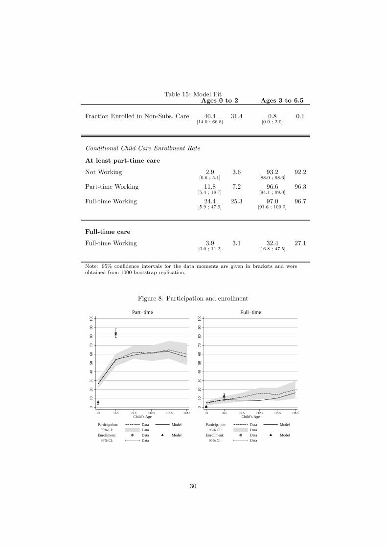
Table 15: Model FitAges 0 to 2 Ages 3 to 6.5

Fraction Enrolled in Non-Subs. Care 40.4 31.4 0.8 0.1[14.0 ; 66.8] [0.0 ; 2.0]

Conditional Child Care Enrollment Rate

At least part-time care

Not Working 2.9 3.6 93.2 92.2[0.6 ; 5.1] [88.0 ; 98.6]

Part-time Working 11.8 7.2 96.6 96.3[5.4 ; 18.7] [94.1 ; 99.0]

Full-time Working 24.4 25.3 97.0 96.7[5.9 ; 47.9] [91.6 ; 100.0]

Full-time care

Full-time Working 3.9 3.1 32.4 27.1[0.0 ; 11.2] [16.8 ; 47.5]

Note: 95% confidence intervals for the data moments are given in brackets and wereobtained from 1000 bootstrap replication.

Figure 8: Participation and enrollment

010

2030

4050

6070

8090

100

<3 <6.5 <9.5 <12.5 <15.5 <18.5Child’s Age

Participation: Data Model

95% CI: Data

Enrollment: Data Model

95% CI: Data

Part−time

010

2030

4050

6070

8090

100

<3 <6.5 <9.5 <12.5 <15.5 <18.5Child’s Age

Participation: Data Model

95% CI: Data

Enrollment: Data Model

95% CI: Data

Full−time

30

Figure 8 shows the part- and full-time participation profiles as the children age.Recall that all moments in periods one, two and six were used as targets. Thereis one exception, namely full-time child care enrollment for children aged zeroto two which is nevertheless matched precisely. The profile of the part-timeparticipation rate is replicated fairly well, whereas for full-time participationthe increase during period three and four (above age six and half until age 15)is not.

31

Figure 9: Participation and enrollment rates by number of children0

1020

3040

5060

7080

9010

0

<3 <6.5 <9.5 <12.5 <15.5 <18.5Child’s Age

Participation: Data Model

95% CI: Data

Enrollment: Data Model

95% CI: Data

1 child

010

2030

4050

6070

8090

100

<3 <6.5 <9.5 <12.5 <15.5 <18.5Child’s Age

Participation: Data Model

95% CI: Data

Enrollment: Data Model

95% CI: Data

2 children

010

2030

4050

6070

8090

100

<3 <6.5 <9.5 <12.5 <15.5 <18.5Child’s Age

Participation: Data Model

95% CI: Data

Enrollment: Data Model

95% CI: Data

3 children

32

In the calibration, average participation and enrollment rates, i.e. the averageover all mothers, were targeted. Another set of overidentifying restrictions isthus given by the participation and enrollment rates by the number of children,shown in Figure 9. For mothers with one child the participation rate is predicted,fairly well whereas enrollment rates fall slightly short. The facts for motherswith two children are replicated closely although the participation rates in periodone and two are overpredicted. The worst fit is obtained for females with threechildren with a substantial underprediction of participation. Figure 10 providesthe split by part- and full-time rates.

The overall participation pattern for females with one child is matched fairlywell. However, while part-time participation is consistently overpredicted theopposite is true for full-time participation. Both part- and full-time participa-tion are predicted precisely for mothers with two children, although they areoverpredicted in period one and two. The worse match for females with threechildren comes both from an underprediction of part- and full-time participa-tion, with an exception of periods one and two.

6 Policy experiments

In this section, I conduct and compare three counterfactual policy experiments.First, since January 2007 females can receive for up to twelve months after birtha monthly maternity leave benefit of 67% of their pre-birth monthly net incomeor 1800e – whatever is less. In this experiment, I replace the initial maternityleave benefit of 2414.19 e granted to all females with children aged zero totwo either not or part-time working with the new policy. Second, I assume thatevery part-time working female has access to subsidized part-time child care andevery full-time working female has access to subsidized child care full-time care.Rationing only occurs for non-working females and part-time working femaleswith respect to full-time care for which I leave the success probabilities of theslot lottery unchanged. The third experiment mimics a political initiative bythe Bavarian conservative party (CSU), who argue the subsidy on child carediscriminates females who prefer to stay at home taking care of their childrenthemselves. After this proposal, non-working mothers who do not use subsidizedchild care while their children are of age one and two receive a monthly subsidyof 150e per child.

Table 16 compares the effects of the three reforms to the baseline model out-come. The larger transfers conditional on not working full-time by the ’07 LeaveBenefits reform naturally decreases the full-time participation rate for childrenaged zero to six while the part-time participation rate is left unchanged. Overall,it is however the case that the extra money drives full-time working women intopart-time and part-time working women out of the labor force. The part-timeparticipation rate itself increases by roughly 5% points in all remaining periodsand the full-time participation by less than that. The fertility rate increases by0.1 children per female through a shift from zero to one and one to two children.

Rationing access to child care by the labor force participation status increasespart-time and full-time employment for mothers of children aged zero to two.However, the increase is only modest compared to the increase in the enrollment

33

Figure 10: Part- and full-time enrollment and participation

010

2030

4050

6070

8090

100

<3 <6.5 <9.5 <12.5 <15.5 <18.5Child’s Age

Participation: Data Model

95% CI: Data

Enrollment: Data Model

95% CI: Data

Part−time

010

2030

4050

6070

8090

100

<3 <6.5 <9.5 <12.5 <15.5 <18.5Child’s Age

Participation: Data Model

95% CI: Data

Enrollment: Data Model

95% CI: Data

Full−time

1 child0

1020

3040

5060

7080

9010

0

<3 <6.5 <9.5 <12.5 <15.5 <18.5Child’s Age

Participation: Data Model

95% CI: Data

Enrollment: Data Model

95% CI: Data

Part−time

010

2030

4050

6070

8090

100

<3 <6.5 <9.5 <12.5 <15.5 <18.5Child’s Age

Participation: Data Model

95% CI: Data

Enrollment: Data Model

95% CI: Data

Full−time

2 children

010

2030

4050

6070

8090

100

<3 <6.5 <9.5 <12.5 <15.5 <18.5Child’s Age

Participation: Data Model

95% CI: Data

Enrollment: Data Model

95% CI: Data

Part−time

010

2030

4050

6070

8090

100

<3 <6.5 <9.5 <12.5 <15.5 <18.5Child’s Age

Participation: Data Model

95% CI: Data

Enrollment: Data Model

95% CI: Data

Full−time

3 children

34

Table 16: Counterfactual Policy Experiments’07 Leave Conditional Cash

Baseline Benefits Rationing Subsidy

Ages 0 to 2

Part-time

Participation 26.2 26.1 30.4 7.6

Enrollment 5.1 8.4 32.4 2.5

Full-time

Participation 5.1 0.0 7.7 5.1

Enrollment 0.6 0.7 8.1 0.3

Ages 3 to 6.5

Part-time

Participation 53.6 58.4 51.2 54.0

Enrollment 81.8 78.7 75.7 83.0

Full-time

Participation 8.7 8.3 11.8 10.2

Enrollment 12.9 17.2 21.8 11.3

Ages 7 to 18.5 (Avg.)

Part-time participation 60.0 65.7 60.5 59.8

Full-time participation 10.6 7.9 10.7 11.5

Fertility Rate 1.78 1.89 1.79 2.04

35

rate. Hence, working mothers substitute non-paid with paid child care and forthe vast majority of non-working mothers the rationing of child care is notresponsible for their decision to stay out of the labor force. Only for a smallfraction of non-working women abolishing the rationing of child care inducesthem to start working. It is worthwhile mentioning that this reform which isclose to the actual implemented one by the federal government would result inan enrollment rate close to the target stated in the introductory quote from theEuropean Council. The full-time participation rate of mothers with childrenaged three to six and a half increases slightly, mainly at the expense of a lowerpart-time participation rate. In the remaining periods, and with respect tofertility, there is hardly any response.

The final experiment subsidizes non-working mothers who do not use child carewhile their children are of ages zero to two. The reform is very effective inreducing the corresponding maternal labor force participation rate. The pos-itive effect is that it has no long-lasting impact in further periods, full-timeparticipation increases even slightly. Among all policy experiments, subsidizingnon-working mothers who do not use child care while their children are of ageszero to two has the largest impact on fertility with an increase of 0.26 childrenper female.

From these results, one can conclude that the provision of subsidized child carehas only very modest effects on maternal labor force participation and fertility.In contrast, monetary incentives raise fertility strongly, essentially without anegative long-lasting impact on labor force participation.

7 Conclusion

In this paper, I documented facts about labor force participation and child careenrollment decisions of married females in West Germany. In line with the factsof a cross-section of OECD countries, I emphasize the level relationship betweenmaternal labor force participation and child care enrollment. While for childrenaged zero to two, the labor force participation rate is by a magnitude largerthan the child care enrollment rate and the opposite is the case for children agedthree to six and a half. I setup a structural life-cycle model with endogenousfertility, labor supply and child care choices that is calibrated to match thesefacts and also provides a good description of data moments not targeted. A setof counterfactual policy experiments indicates that the quantitative impact ofproviding (subsidized) child care on labor force participation and fertility is verysmall whereas financial support is more effective in stimulating fertility withoutdecreasing labor force participation in the long run. Since the analysis focuseson females in long-term relationships, future research should attempt to enrichthe model by marriage and divorce decision in order to generalize the results.

36

References

Apps, P. and Rees, R. (2005). Gender, time use and public policy over the lifecycle, Discussion paper, IZA.

Attanasio, O., Low, H. and Sanchez-Marcos, V. (2008). Explaining Changes inFemale Labor Supply in a Life-Cycle Model, American Economic Review98(4): 1517–1542.

Domeij, D. and Klein, P. (2009). Should day care be subsidized?, Working

paper, Stockholm School of Economics.

European Council Barcelona - Conclusions of the Presidency (2002). Bulletin,European Parliament.

Francesconi, M. (2002). A Joint Dynamic Model of Fertility and Work of MarriedWomen, Journal of Labor Economics 20(2): 336–380.

Greenwood, J., Guner, N. and Knowles, J. A. (2003). More on marriage, fertilityand the distribution of income, International Economic Review 44(3): 827–826.

Haan, P. and Wrohlich, K. (2009). Can child care policy encourage employmentand fertility? evidence from a structural model, Working paper, IZA.

Hotz, V. J. and Miller, R. A. (1988). An empirical analysis of life cycle fertilityand female labor supply, Econometrica 56(1): 91–118.

Jones, L. E., Schoonbroodt, A. and Tertilt, M. (2008). Fertility theories: Canthey explain the negative fertility-income relationship?, Working paper,University of Minnesota.

Kolvenbach, F.-J., Haustein, T., Krieger, S., Seewald, H. and Weber, T. (2004).Kindertagesbetreuung in deutschland, Report, Statistisches Bundesamt.

Kreyenfeld, M. (2001). Employment and fertility - east germany in the 1990s,Dissertation, University of Rostock.

Kreyenfeld, M., Spieß, K. and Wagner, G. G. (2002). Kinderbetreuungspolitikin Deutschland, Zeitschrift fur Erziehungswissenschaft 5(2): 201–221.

Kydland, F. E. and Prescott, E. C. (1982). Time to Build and AggregateFluctuations, Econometrica 50: 1345–1370.

Ludsteck, J. and Schonberg, U. (2007). Maternity leave legislation, female laborsupply, and the family wage gap, Working paper, IZA.

Mincer, J. (1974). Schooling, Experience and Earnings, New York: NationalBureau of Economic Research.

Regalia, F. and Rios-Rull, J.-V. (2001). What accounts for the increase in thenumber of single households, Working paper, University of Pennsylvania.

Robert-Koch-Institut and Statistisches-Bundesamt (2004). Ungewollte kinder-losigkeit, Gesundheitsberichterstattung des Bundes 20.

37

Tauchen, G. (1986). Finite State Markov-Chain Approximations to Univariateand Vector Autoregressions, Economic Letters 20: 177–181.

Wrohlich, K. (2006). Labor supply and child care choices in a rationed childcare market, Working paper, IZA.

Wrohlich, K. (2008). The excess demand for subsidized child care in Germany,Applied Economics 40: 1217–1228.

38

A Data

Table 17: Sample SelectionFrequency

Criterion Absolute Relative

West German, born 1955-1975 4921 100.0%

No move to East German territory 4881 99.2%

Mothers 2868 58.8%

Childless 2013 41.2%

Mothers 2868 100.0%

Births only in relationships 2276 79.4%

Births only in one relationships 2238 78.0%

Relationship intact at last interview 1938 67.6%

Childless 2013 100.0%

At least age forty at last interview 424 21.1%and in a relationship at age forty

Relationship intact at last interview 177 8.8%

Source: GSOEP 1984-2006.

A.1 Sample Construction

A.1.1 Period Definition

Ages 0 to 2 I exclude the month of birth and the subsequent two months toaccount for the mandatory maternity leave which outlaws females to work inthe first eight weeks after the child is born. Depending on when the child isborn within a month this implies an exclusion of the first eight to 13 weeks ofa child’s life. Thus, it is guaranteed that only the months in which it is legallyallowed to work contribute.16 Hence, by construction this period has a durationof 2.75 years.

Ages 3 to 6.5 The second period lasts from the month in which the childturns three until school entry. According to a cut-off rule, which is very similaracross all German states, children who are at least six in July of a given yearhave to enter mandatory schooling. There are exceptions permitting a child to

16Excluding only the month in which a child is born and the next month would correspondto the first five to nine weeks.

39

enter school one year earlier or later. Because of some peculiarities in the timingof the survey the age at school entry cannot always be determined exactly andhas to be constructed. I therefore assume that for all children the cut-off datedetermines school entry but allow children to enter school earlier if this is knownfrom the survey. Even if the exact entry age would be known, the length of theperiod is heterogenous among children because school starts only once a year.The mean duration in the data is 3.5 years.

A.1.2 Child Care

Child Care Enrollment Imputation Information on the child care enroll-ment status for each child is only available at the interview date and is thereforeimputed for the other months of the year based on the following reasoning: Sinceschool starts at the same time for all children, the oldest cohort in a daycarecenter usually leaves the daycare center together at the same time of the year,i.e. at the end of the first half of the year. Therefore the majority of entries intodaycare centers occurs at the beginning of the second half of the year. Hence,the child care enrollment status in the first half of a year is a good predictorfor the status in the second half of the previous year. Similarly, the child careenrollment status in the second half of a year is a good predictor for the childcare enrollment status in first half of the next year. In the following the detailedimputation procedure will be described. The child care enrollment status in theinterview month is assumed to be the same in all other months of a half year.The second half of a year and the first half of the next year have the same statusin case no new information is available. To make that point more clearly, if theinterview month is in the first half of the year, which is the case for more than90% of the interviews, I use this child care enrollment status also for the secondhalf of the previous year if no interview has been conducted in the second halfof the previous year. Analogously, if the interview month is in the second halfof the year I use this child care enrollment status also for the first half of thenext year if no interview is conducted in the first half of the next year. Finally,in all other cases the last known child care enrollment status is used until oneof the two described situation occurs. Although this reasoning applies more tochild care provided in daycare centers, I use the same imputation rule for childcare provided by nannies.

Subsidized Child Care Slot Provsion The slot provision rates are calculatedfrom the data provided by German Statistical Office (Statistik der Jugendhilfe,various years). They are only available for every fourth year between 1986 and2002. Table 19 shows the annual averages over the years 1983 to 2006, the periodfor which the monthly labor supply status from the GSOEP is available. Theseaverages are constructed for the two age groups zero to two, and three to six andhalf as follows: Years before the earliest observation of the slot provision rates,i.e. 1983 to 1985, will be assigned the same value as the first observation of theslot provision rate (1986). Similarly, years after the last observation, i.e. 2003to 2006, will be assigned the same value as the last observation (2002). For theyears between two observations the mean of the corresponding two observationswill be used. The overall provision rates are then obtained as the mean over allyears. From 1994 onwards the provision rates can be further distinguished by

40

part- and full-time from which the fraction of full-time slots from all slots, thefull-time share, will be calculated. As for the overall provision rate, the full-timeshare before the first and after the last observed data points are extrapolatedand between two observation interpolated. The annual provision rate of part-and full-time slot is then given by the provision rate of slots times the fractionof part- or full-time slots from all slots. The mean over all these years thenfinally gives the average provision rate of part- and full-time slots.

These latter rates are used to construct the success probabilities for the slotlottery. If a female would have only one draw from the slot lottery at age zeroand age three, the provision rates could be immediately used as model input.There is however no way to determine how often mothers apply for a slot withina period and a period is regarded as a unified entity. I therefore transform theobserved provision rates into period equivalents in the following way: As alreadydescribed for the imputation of the child care status, the majority of entries intodaycare centers happens once a year. In addition, new information on the childcare enrollment status is usually only once a year available. Therefore I assumethat a female can apply once per year for a slot. If she gets a slot, she can sendher child there until it reaches age three and has to apply again for a slot orgoes to school. Put differently, in each year a female can draw once from thelottery and a successful draw implies that the slot is open for the remainderof the period, i.e. until age three is reached or the child enters school. Once afull-time slot is drawn, the female does not have to redraw until the end of theperiod. Drawing a part-time slot implies that the female can redraw but successis then defined only as drawing a full-time slot because she already has accessto a part-time slot for the rest of the period. Since a model period correspondsto three years I assume that within a period there is a maximum of three drawswhich leads to the set of possible access histories displayed in the left panel ofTable 18.

Table 18: Access to Subsidized Child Care

Access in Year Period Access History1 2 3 Mean Status Probability

No No No 0 No (1 − PP − PF )3

No No Part 1/6 No (1 − PP − PF )2PP

No No Full 1/3 Part (1 − PP − PF )2PF

No Part Part 1/3 Part (1 − PP − PF )PP (1 − PF )

No Part Full 1/2 Part (1 − PP − PF )PPPF

No Full Full 2/3 Part (1 − PP − PF )PF

Part Part Part 1/2 Part PP (1 − PF )2

Part Part Full 2/3 Part PP (1 − PF )PF

Part Full Full 5/6 Full PPPF

Full Full Full 1 Full PF

41

Consider the case that a female would always use as much subsidized childcare as she can get access to. In line with the definition for period child careenrollment status in each year no slot is assigned a 0, part- and full-time slotswith 0.5 and 1. The mean over the whole period - the three years - would begiven in column 4 in Table 18 whereas column 5 corresponds to the associatedchild care enrollment status for each possible access history using the samethresholds as before (0.25 and 0.75). Since I assume that a female does nothave to use the slot she has drawn access to for some part of the period or atall, columns 4 and 5 state the period access status as opposed to the periodenrollment status. Column 6 displays the probability of observing a specificaccess history. PP and PF are the probabilities of drawing a part- or full-timeslot in a given year and correspond to the observed slot provision rates whichdiffer by age. Finally, the probability for having access to no, a part- or full-timeslot over the whole period is equal to the sum of the history probabilities that areassociated with the respective period access status. For example, the probabilityto have no slot as defined by the period access status would be the sum overthe two first histories ([No, No, No]; [No, No, Part-time]) and equal to(1−PP −PF )3 +(1−PP −PF )2PP . Table 19 presents the annual, i.e. observed,slot provision rates and the period provision rates after the transformation. E.g.while there are 62.3 part-time and 14.6 full-time slots per 100 children aged threeto six and a half, the probability for a female that she has access to a part-timeslot over the whole period where the child is between age three and six and a halfis 71.8% and 23.7% for a full-time slot. Note that by construction, the periodprovision rates have to be larger than the annual/observed provision rates. Thisis also the case for children aged zero to two for the non-rounded numbers.

Table 19: Annual and Period Provision Ratesof Subsidized Child Care Slots

West EastAnnual Period Annual Period

Ages 0 to 2

Part-time 0.5 4.3 1.2 38.8⇒ ⇒

Full-time 1.7 1.7 40.6 41.1

Ages 3 to 6.5

Part-time 62.3 71.8 1.8 2.4⇒ ⇒

Full-time 14.6 23.7 95.9 97.6

B Model

42

Table 20: Minimum distance to one of the own parents or parents in lawAges 0 to 2 Ages 3 to 6.5

Same house 35.6 60.8[25.7 ; 45.5] [50.2 ; 71.4]

Same neigbourhood 38.7 64.2[30.3 ; 47.1] [55.4 ; 72.9]

Same city 31.5 63.3[23.5 ; 39.5] [54.4 ; 72.2]

Within 1h driving distance 36.1 59.8[28.1 ; 44.1] [51.4 ; 68.3]

Farther away 26.5 66.0[16.0 ; 37.0] [52.7 ; 79.3]

Source: GSOEP, 1991, 1996 and 2001.

Note: 95% confidence intervals are given in brackets and were obtainedfrom 1000 bootstrap replication.

43