The Productivity of Agricultural Credit in India · 2015-01-23 · The Productivity of Agricultural Credit in India ... in response to the persistent problem of indebtedness and to

WP-2015-01

The Productivity of Agricultural Credit in India

Sudha Narayanan

Indira Gandhi Institute of Development Research, MumbaiJanuary 2015

http://www.igidr.ac.in/pdf/publication/WP-2015-01.pdf


Sudha NarayananIndira Gandhi Institute of Development Research (IGIDR)

General Arun Kumar Vaidya Marg Goregaon (E), Mumbai- 400065, INDIA

Email(corresponding author): [email protected]

AbstractThis study examines the nature of the relationship between formal agricultural credit and agricultural

GDP in India, specifically the role of the former in supporting agricultural growth, using state level

panel data covering the period 1995-96 to 2011-12. The study uses a mediation analysis framework to

map the pathways through which institutional credit relates to agricultural GDP relying on a control

function approach to tackle the problem of endogeneity. The findings from the analysis suggest that

over this period, all the inputs are highly responsive to an increase in institutional credit to agriculture.

A 10 % increase in credit flow in nominal terms leads to an increase by 1.7% in fertilizers (N, P, K)

consumption in physical quantities, 5.1% increase in the tonnes of pesticides, 10.8% increase in tractor

purchases. Overall, it is quite clear that input use is sensitive to credit flow, whereas GDP of agriculture

is not. Credit seems therefore to be an enabling input, but one whose effectiveness is undermined by low

technical efficiency and productivity. Notwithstanding these aggregate findings detailed microstudies

would be necessary to provide insights into this issue.

Keywords: agricultural credit, growth, control function, elasticity, India

JEL Code: Q10, Q14

Acknowledgements:

This study was funded by the Research and Development (R&D) fund of the Department of Economic Analysis and Research

(DEAR), NABARD. I thank Dr. Harsh Kumar Bhanwala, Chairman, NABARD, Dr.Prakash Bakshi, Former Chairman,

NABARD, Dr.R.N.Kulkarni, Dr.M.V.Ashok, Dr.Satyasai, the DEAR team at NABARD and Dr.S.Mahendra Dev for their

support advice and inputs at various stages of this work. Garima Dhir provided valuable research assistance. Andaleeb Rahman,

Krushna Ranaware, Sowmya Dhanraj, Sanjay Prasad, Sumit Mishra and others assisted in putting together the dataset used for this

study. This work has benefitted immensely from Nirupam Mehrotra's inputs and insights into the various issues relating to the role

of credit in Indian agriculture. I also thank all the participants of seminars on July 4, 2013 and November 14, 2014 at DEAR,

NABARD and Pallavi Chavan of the RBI. A number of their suggestions have been incorporated in this paper. All remaining

errors and omissions are however mine.

1


Sudha Narayanan1

Abstract

This study examines the nature of the relationship between formal agricultural credit and

agricultural GDP in India, specifically the role of the former in supporting agricultural growth, using

state level panel data covering the period 1995-96 to 2011-12. The study uses a mediation analysis

framework to map the pathways through which institutional credit relates to agricultural GDP

relying on a control function approach to tackle the problem of endogeneity. The findings from the

analysis suggest that over this period, all the inputs are highly responsive to an increase in

institutional credit to agriculture. A 10 % increase in credit flow in nominal terms leads to an

increase by 1.7% in fertilizers (N, P, K) consumption in physical quantities, 5.1% increase in the

tonnes of pesticides, 10.8% increase in tractor purchases. Overall, it is quite clear that input use is

sensitive to credit flow, whereas GDP of agriculture is not. Credit seems therefore to be an enabling

input, but one whose effectiveness is undermined by low technical efficiency and productivity.

Notwithstanding these aggregate findings detailed microstudies would be necessary to provide

insights into this issue.

Keywords: agricultural credit, growth, control function, elasticity, India

JEL Classification Q10, Q14

1Assistant Professor, IGIDR , [email protected]

2

ACKNOWLEDGEMENTS

This study was funded by the Research and Development (R&D) fund of the Department of

Economic Analysis and Research (DEAR), NABARD. I thank Dr. Harsh Kumar Bhanwala,

Chairman, NABARD, Dr.Prakash Bakshi, Former Chairman, NABARD, Dr.R.N.Kulkarni,

Dr.M.V.Ashok, Dr.Satyasai, the DEAR team at NABARD and Dr.S.Mahendra Dev for their

support advice and inputs at various stages of this work. Garima Dhir provided valuable

research assistance. Andaleeb Rahman, Krushna Ranaware, Sowmya Dhanraj, Sanjay

Prasad, Sumit Mishra and others assisted in putting together the dataset used for this

study. This work has benefitted immensely from Nirupam Mehrotra’s inputs and insights

into the various issues relating to the role of credit in Indian agriculture. I also thank all the

participants of seminars on July 4, 2013 and November 14, 2014 at DEAR, NABARD and

Pallavi Chavan of the RBI. A number of their suggestions have been incorporated in this

paper. All remaining errors and omissions are however mine.

3


1. Introduction

The decades since 1990 have been challenging times for Indian agriculture. Growth rates of

agricultural Gross Domestic Product (GDP) have been languishing and the traditional crop sectors

have seen declining profitability. This has pushed policy makers to direct special attention to

addressing some of the pressing concerns confronting Indian agriculture. Institutional credit has

been an important lever in this effort. Indeed, as many as three major policy initiatives focussed on

institutional credit have been implemented since 2000 to bolster the agricultural sector. The first

policy initiative, introduced in 2004-05, was to double the volume of credit to agriculture over a

period of three years (to 2006-07), relative to the 2004-05 base to expand the reach of formal

finance. Close on its heels came the Agricultural Debt Waiver and Debt Relief Scheme (ADWDRS)

2008, in response to the persistent problem of indebtedness and to alleviate financial pressures

faced by the farmers. The interest rate subvention was then introduced in 2010-11 with the stated

goal of providing incentives for prompt repayment of loans, partly to address the perceived fallout

of the ADWDRS, that it had somehow vitiated the repayment culture. All three measures have

contributed, both explicitly and implicitly, to burgeoning institutional lending to agriculture in the

last decade.2

Despite the significance of these interventions, very little is known regarding the outcomes,

in particular, whether institutional credit has had the intended impact on agricultural growth.

Existing commentaries focussing on this period point out the poor correlation between the two

(Chavan and Ramakumar, 2007 for example). In this context, this research project aims to

understand the extent to which, if at all, growing institutional credit to agriculture supports growth

in the sector. What is its precise role and through what pathways does it support agriculture? These

questions assume particular significance in the context of recent speculation that agricultural credit

might not entirely flow to agriculture or and that there is a significant spillover to other sectors

(Chavan, 2009; Burgess and Pande, 2005 and Binswanger and Khandker, 1992). Some ask if formal

credit a `sensible’ way to support agriculture in India. While answers to this question are perhaps

addressed best through detailed microstudies, it is also possible to elicit patterns and relationships

between agricultural credit and agricultural GDP using secondary data. This study uses secondary

data to examine four specific questions: How productive is institutional credit to the agricultural

sector? What has been the trend since mid-1990s? What are the pathways through which credit

impacts agriculture? How, if at all, have these pathways changed over the years? Using detailed

state level data for the period 1995-2012, we analyze the possible impact of credit on agricultural

GDP using multiple methods, using a control function approach. We also analyse the potential

pathways through which institutional credit can influence agricultural growth, focussing on the

responsiveness of input demand to institutional credit flow in some detail. An aggregate analysis of

this nature necessarily has severe limitations and needs to be interpreted with care but can serve to

complement our understanding of the productivity of agricultural credit in India.

2 There is evidence to suggest that the institutional lending to agriculture might have picked up since 2000, even before the doubling of credit in 2004-05 (Chavan and Ramakumar, 2007).

4

The paper is organized as follows. The following section (Section 2) provides the context of

agriculture and credit in recent times, underscoring the motivation for this study. Section 3 reviews

the empirical evidence on the productivity of rural credit in India, focussing on secondary data

analysis at the aggregate level (state or national). Section 4 provides a conceptual framework for

the present analysis. Section 5 then discusses the empirical strategies adopted in this work to tackle

some inherent econometric issues that pose problems for establishing a causal relationship

between credit and agricultural GDP. The section discusses the data used for the analysis and also

outlines the scope and limitations of these approaches. Section 6 is devoted to the results from the

econometric exercise and discusses the findings at length. The concluding section 7 closes with

some remarks on the study and the way forward.

2. Characterizing Agriculture and Institutional Credit since the 1990s.

Both the structure of agriculture and the nature of institutional credit have been undergoing a

rapid change since the 1990s but became especially pronounced since 2000. Initiatives to expand

the reach of formal credit has been a goal pursued consistently in the past mainly by designating

agriculture as a priority sector for lending. The introduction of schemes such as the Kisan Credit

Card (KCC) scheme in 1998-99 aimed to provide farmers with adequate and timely credit support

from the banking system for agriculture and allied activities in a flexible and cost-effective manner.

Three major policy initiatives in recent years have come to define the context of institutional

credit to agriculture in India, as outlined in the introduction. The first policy introduced in 2004

sought to double the volume of agricultural credit relative to what it was in 2004-05, over a period

of three years. Since then, the actual credit flow has consistently exceeded the target (Government

of India, 2012). Against a credit flow target of Rs.3,25,000 crore during 2009-10, the achievement

was Rs.3,84,514 crore, forming 118 percent of the target. The target for 2010-11 was Rs.3,75,000

crore while the achievement on March, 2011 is Rs.4,46,779 crore (Government of India ,2013). A

second policy involved the waiving of agricultural debt for small farmers and an opportunity for

one time settlement for others.3 Close on its heels, an interest subvention scheme was introduced to

reward prompt repayment of loans, widely perceived has having been vitiated by the debt waiver

scheme. Under the existing interest subvention scheme, farmers get short-term crop loans at seven

per cent interest. If the loan to the bank is promptly paid then the effective rate of interest to the

farmer works out to four per cent a year due to the additional interest subvention.4 Interest

subvention scheme for short-term crop loans to be continued scheme extended for crop loans

borrowed from private sector scheduled commercial banks. Together, these interventions have

both explicitly and implicitly transferred large amounts to the agricultural sector. Although the

increasing trend of institutional credit flow might have begun in 2000 itself (Ramakumar and

3As per the provisional figures, a total of 3.01 crore small and marginal farmers and 67 lakh 'other farmers' have benefited from the Scheme involving debt waiver and debtrelief of Rs.65,318.33crore (Government of India, 2013). 4From kharif 2006-07, farmers are receiving crop loans upto a principal amount of 3 lakh at 7% rate of interest. In the year 2009-10, Government provided an additional 1% interest subvention to those farmers who repaid their short term crop loans as per schedule. This subvention for timely repayment of crop loans was raised from 1% to 2% in 2010-11, further 3% from the year 2011-12. Thus the effective rate of interest for such farmers will be 4 % p.a. (Government of India, 2013).

5

Chavan, 2007), credit flow in recent years have stood out for its magnitude, if not for reversing the

trend of the 1990s.

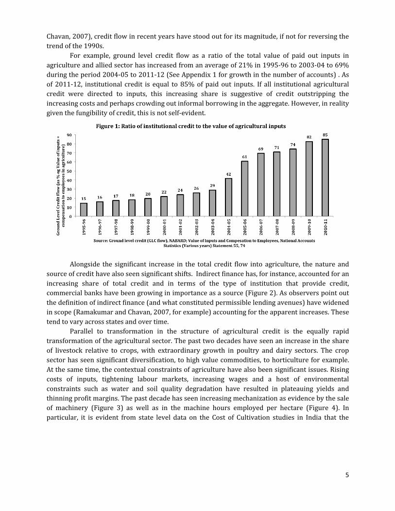
For example, ground level credit flow as a ratio of the total value of paid out inputs in

agriculture and allied sector has increased from an average of 21% in 1995-96 to 2003-04 to 69%

during the period 2004-05 to 2011-12 (See Appendix 1 for growth in the number of accounts) . As

of 2011-12, institutional credit is equal to 85% of paid out inputs. If all institutional agricultural

credit were directed to inputs, this increasing share is suggestive of credit outstripping the

increasing costs and perhaps crowding out informal borrowing in the aggregate. However, in reality

given the fungibility of credit, this is not self-evident.

Alongside the significant increase in the total credit flow into agriculture, the nature and

source of credit have also seen significant shifts. Indirect finance has, for instance, accounted for an

increasing share of total credit and in terms of the type of institution that provide credit,

commercial banks have been growing in importance as a source (Figure 2). As observers point out

the definition of indirect finance (and what constituted permissible lending avenues) have widened

in scope (Ramakumar and Chavan, 2007, for example) accounting for the apparent increases. These

tend to vary across states and over time.

Parallel to transformation in the structure of agricultural credit is the equally rapid

transformation of the agricultural sector. The past two decades have seen an increase in the share

of livestock relative to crops, with extraordinary growth in poultry and dairy sectors. The crop

sector has seen significant diversification, to high value commodities, to horticulture for example.

At the same time, the contextual constraints of agriculture have also been significant issues. Rising

costs of inputs, tightening labour markets, increasing wages and a host of environmental

constraints such as water and soil quality degradation have resulted in plateauing yields and

thinning profit margins. The past decade has seen increasing mechanization as evidence by the sale

of machinery (Figure 3) as well as in the machine hours employed per hectare (Figure 4). In

particular, it is evident from state level data on the Cost of Cultivation studies in India that the

6

mechanization process has replaced animal and draught power while decline in human labour

inputs into agriculture have been less by comparison (Figure 4). 5

5 For more details on cost of cultivation studies in India, see http://eands.dacnet.nic.in/Cost_of_Cultivation.htm. Accessed January, 2014.

7

Source: Cost of Cultivation in India (several years). The All India average is the weighted avearge

across crops and states, where the weights are area sown under each crop within state and the net

sown area across states.

There is now limited evidence that despite the widespread notion of a crisis, Indian

agriculture might be more productive but that these improvements as represented by Total Factor

Productivity (TFP) is coming from certain states (in the south and west) and certain sectors (such

as horticulture and livestock).6 Other evidence similarly suggests that productivity improvements

is marked only in a few states (Chaudhari, 2013). Improvements in efficiency are low for a majority

of states and might have in fact declined in several states implying the presence of potential gains in

production even with existing technology.

The links that institutional credit has to agricultural productivity and growth are still

somewhat underresearched. Figure 5 plots the ratio of agricultural GDP to credit flow over the

period 1996-2011 for the various states. It is apparent that notwithstanding the variation across

states, the ratio for the country as a whole has been declining over the past 15 years and is now

close to one on average. These patterns appear to indicate that although credit is contributing to a

larger share of the value of purchased inputs, the relationship between agricultural GDP and

agricultural credit are possibly weak, raising important questions on the role of agricultural credit.

Figure 5: The Ratio of Agricultural GDP and Credit for major states (1996-2011)

6See Rada(2013) for a recent analysis of Total Factor Productivity in India. Results suggest renewed growth in aggregate TFP growth despite a slowdown in cereal grain yield growth. TFP growth appears to have shifted to the Indian South and West, led by growth in horticultural and livestock products over the period 1980-2008.

8

Notes: The scatter points represent the ratio of agricultural GDP and credit outflow and the line

represent the lowess fit, i.e. locally weighted scatterplot smoothing.

3. Empirical Evidence on the Productivity of Institutional Credit in India

The best known study of the impact of formal rural credit in the context of India is by

Binswanger and Khandkher (1992) who found that rural credit has a measurable positive effect on

agricultural output. Cooperative credit advanced has elasticity with respect to output of 0.063. It is

larger than the elasticity of crop output with respect to predicted overall rural credit which is near

0.027, but not precisely estimated. The estimate for the impact of commercial bank branches on

output is more precisely estimated at 0.02. Others suggest that the effect on output is either non-

existent, for example Burgess and Pande (2005) who claim that the increase in output due to formal

credit comes entirely from increases in non-farm output, or have been negligible.7 Others show that

there is a positive association between credit and agricultural output but that this varies cross

states and further that there is a positive association between the number of persons with accounts

and agricultural output suggesting the financial inclusion could impact agricultural output

positively (Das, et al, 2009).8 However a dynamic panel data estimation of this relationship does

7The estimates suggested that a one percent increase in the number of rural banked locations reduced rural poverty by roughly 0.4 percent and increased total output by 0.30 percent. The output effects are solely accounted for by increases in non-agricultural output – a finding which suggests that increased financial intermediation in rural India aided output and employment diversification out of agriculture. 8There are two models that have been estimated in the literature - fixed effects and random effects. The fixed effects model assumes that there is an unobserved time independent effect for each state of India and this effect could be correlated with other explanatory variables. The Hausman test helps decide whether to

9

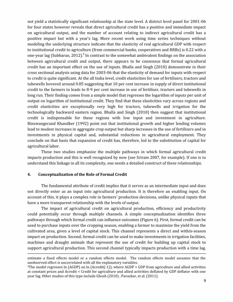
not yield a statistically significant relationship at the state level. A district level panel for 2001-06

for four states however reveals that direct agricultural credit has a positive and immediate impact

on agricultural output, and the number of account relating to indirect agricultural credit has a

positive impact but with a year’s lag. More recent work using time series techniques without

modeling the underlying structure indicate that the elasticity of real agricultural GDP with respect

to institutional credit to agriculture (from commercial banks, cooperatives and RRBs) is 0.22 with a

one-year lag (Subbarao, 2012).9 In contrast to the somewhat ambivalent findings on the association

between agircultural credit and output, there appears to be consensus that formal agricultural

credit has an important effect on the use of inputs. Bhalla and Singh (2010) demonstrate in their

cross sectional analysis using data for 2003-06 that the elasticity of demand for inputs with respect

to credit is quite significant. At the all India level, credit elasticities for use of fertilisers, tractors and

tubewells hovered around 0.85 suggesting that 10 per cent increase in supply of direct institutional

credit to the farmers to leads to 8-9 per cent increase in use of fertiliser, tractors and tubewells in

long run. Their finding comes from a simple model that regresses the logarithm of inputs per unit of

output on logarithm of institutional credit. They find that these elasticities vary across regions and

credit elasticities are exceptionally very high for tractors, tubewells and irrigation for the

technologically backward eastern region. Bhalla and Singh (2010) then suggest that institutional

credit is indispensable for these regions with low input and investment in agriculture.

Binswangerand Khandker (1992) point out that institutional growth and higher lending volumes

lead to modest increases in aggregate crop output but sharp increases in the use of fertilizers and in

investments in physical capital and, substantial reductions in agricultural employment. They

conclude on that basis that expansion of credit has, therefore, led to the substitution of capital for

agricultural labor.

These two studies emphasize the multiple pathways in which formal agricultural credit

impacts production and this is well recognized by now (see Sriram 2007, for example). If one is to

understand this linkage in all its complexity, one needs a detailed construct of these relationships.

4. Conceptualization of the Role of Formal Credit

The fundamental attribute of credit implies that it serves as an intermediate input and does

not directly enter as an input into agricultural production. It is therefore an enabling input. On

account of this, it plays a complex role in farmers’ production decisions, unlike physical inputs that

have a more transparent relationship with the levels of output.

The impact of agricultural credit on agricultural production, efficiency and productivity

could potentially occur through multiple channels. A simple conceptualization identifies three

pathways through which formal credit can influence outcomes (Figure 6). First, formal credit can be

used to purchase inputs over the cropping season, enabling a farmer to maximize the yield from the

cultivated area, given a level of capital stock. This channel represents a direct and within-season

impact on production. Second, formal credit can be used to make investments in irrigation facilities,

machines and draught animals that represent the use of credit for building up capital stock to

support agricultural production. This second channel typically impacts production with a time lag. estimate a fixed effects model or a random effects model. The random effects model assumes that the unobserved effect is uncorrelated with all the explanatory variables. 9The model regresses ln (AGDP) on ln (Acredit(-1)), where AGDP = GDP from agriculture and allied activities at constant prices and Acredit = Credit for agriculture and allied activities deflated by GDP deflator with one year lag. Other studies of this type include Ghosh (2010) , Pavaskar, et al. (2011).

10

Both of these represent a “liquidity effect” (Binswanger and Khandkher, 1992) since they relieve a

farmer’s credit constraint and enables purchase of critical inputs to support production. Third,

formal credit is often used to replace informal credit associated with high interest burden.

Anecdotal evidence suggests that farmers often borrow from formal sources to pay off high interest

loans taken from money lenders. This has the effect of relieving credit constraints, reducing the

interest burden and indebtedness. Existing economic literature on wealth effects and risk aversion

suggests that this often enables farmers to make decisions that increase profitability and efficiency.

Even when formal credit is diverted to consumption, there could be an implicit wealth effect that

impacts farmer’s production decisions. This last channel, which incorporates a “consumption

smoothing” effect is is often difficult to capture.

Collectively, formal agricultural credit can be regarded as having two kinds of impacts –

first, it could enable a farmer to move to the production frontier so that given prevalent technology,

a farmer is using levels of inputs that enable him/her to produce at the frontier, from among many

feasible combinations of crops. Second, it could enable a farmer to move on to a superior

production frontier, so that given a level of inputs, the farmer is able to produce more of one or

more of the crops. The first is represented as a move from within the production possibility set to

the frontier (constituting efficiency improvement) and the second is represented as a shift of the

frontier itself (constituting productivity improvement). The impact of formal agricultural credit on

agricultural output conflates these two aspects of productivity and efficiency effects.

Direct Credit from

formal institutions

“Consumption Smoothing Effect” Replace usurious loans, relax consumption constraints, etc.increasing the risk-bearing capacity of farmers.

“Liquidity Effect” 1: Working Capital (for purchase of inputs)

“Liquidity Effect” 2: Investment credit (for purchase of `capital stock’ to support production)

Agricultural

Production

Figure 6 : Schematic Representation of Pathways

11

5. Empirical Strategy

a. The Challenges

Empirically, these effects are difficult to entangle. While a separation of these effects and

pathways are ideally studied at the household level, this logic can be extended to an aggregate level

by choosing empirical counterparts that represent these dimensions at the state or district level,

with important caveats. Aggregation often masks a lot of the heterogeneity and complexity of the

ways in which formal agricultural mediates production processes. The distribution of credit among

farmers or farmer groups is often uneven and is not taken into account when in an aggregate

analysis. Similar problems occur with aggregating over all the crops and commodities, which

masks the differential impacts and relative importance of credit. While this study is cognizant of

these issues, data limitations allow only an aggregate-level analysis.

Several methodological and data challenges persist in estimating the impact of formal

agricultural credit on output, especially at the aggregate level. Firstly, informal credit which forms a

major source of credit is something of a black box with virtually no data available on its quantum or

how it is used. The fungibility of credit too poses difficult problems for research since it makes

short and long term credit indistinguishable at the farmers’ end. Similarly there could be spillovers

into non-farm sector that are unknown to the lenders and to researchers. Direct and Indirect

finance might also not be watertight categories so that it could be the case that direct credit to the

farmer is in fact used for ancillary activities that support agriculture. All of these make it hard to pin

down the precise nature of relationship between credit and agriculture. Further, the dynamic

effects are difficult to capture since credit flow in a particular year might yield cumulative benefits

over several years. This is particularly difficult to model. The other major challenges stem from data

constraints at the state level. Existing data for variables of interest are not often available for all the

states and for all the years, forcing us to confine the analysis to the states for which we have

complete data for the period of focus.

The empirical challenges of studying the relationship between formal agricultural credit

and output at an aggregate level are best described by Binswanger and Khandker (1992). The first

problem is the joint determination of both observed formal credit to agriculture and aggregate

output. The second problem emanates from the absence of data on informal credit, which makes it

difficult to capture the impacts of formal credit that might work through reduced informal

borrowing, and not factoring this might yield the estimates that reflect the true effect of formal

credit. Credit advanced by formal lending agencies such as banks is an outcome of both the supply

of and demand for formal credit. The amount of formal credit available to the farmer, his/her credit

ration, enters into his/her decision to make investments, and to finance and use variable inputs

such as fertilizer and labor. The third econometric problem arises because formal agriculture

lending is not exogenously given or randomly distributed across space. Ways to be able to address

some of these issues are central concerns of this study.

12

b. Methodology

To parse this complex relationship given the limitations of data, a combination of three

approaches are used (Box 1). The first is a simple model that regresses agricultural GDP on credit

flow using state level data. This is a catchall approach that cannot comment on the pathways or

provide a causal interpretation. The second method estimates a hybrid profit-production function

that regresses agricultural GDP on a vector of relevant inputs, prices and agricultural credit for the

same year. This is a direct approach to estimating the relationship between credit and agricultural

GDP in reduced form. The possible endogeneity of credit is addressed by the use of a control

function approach where a regression function is estimated that identified and then “controls” for

the endogenous component of observed credit flow (Imbens and Wooldridge, 2007). The coefficient

on credit in this case captures one dimension of impact of credit that is not mediated through

inputs. The third method is perhaps the most comprehensive and models the pathways approach in

what is referred to as a mediation analysis framework, where inputs are regarded as mediating the

relationship between institutional credit and agricultural

GDP (Preacher and Hayes, 2008). Here, a set of regressions

estimates input demand as a function of credit, among

other things and controlling for endogeneity of credit

(indirect effect), and the hybrid production-profit function

as a function of inputs and credit, recognizing that credit

can also have direct effect on GDP. The coefficients

representing the responsiveness of input use to

institutional credit are therefore used as components to

construct the total impact of agricultural credit on

agricultural GDP (Preacher and Hayes, 2008). The impact

of credit on agricultural output is thus derived as the sum

of the contribution of credit to the use of specific inputs,

capital or the cropping pattern, weighted by the

contribution of these to the total value of agricultural

production. These are estimated in a Seemingly Unrelated

Regression Equations (SURE) framework that

acknowledges the potential interrelationship between

these variables and the fact that they might be jointly

determined. Appendix 2 contains a representation of the models estimated.

For all three methods we use state-level data to estimate the relevant parameters of interest

for India as a whole. The analysis pertains to the time period 1995-96 to 2011-12, for which the

data is complete. Further, we also perform an analysis for two sub-periods first (1995-96 to 2003-

04) and post doubling (2004-05 to 2011-12). In all the methods, we make the assumption of

constant elasticity of demand, which is in fact a non-trivial assumption, but one that is typical of

studies of this kind.

As mentioned earlier, the chief methodological challenge involves dealing with the the issue

of endogeneity of observed credit. There are several approaches to deal with this. One approach to

tackle the endogeneity of observed volumes of credit is to use the predicted supply of credit at the

state level, following Binswanger and Khandker (1992) or to use lagged credit that is correlated

with current year credit. Each of these involves a set of defensible assumptions. The latter approach

Box 1: The Three Approaches

Method 1: The Simple Model using

state level data and dividing into time

periods in nominal terms as well as

accounting for prices.

Method 2: The Direct Approach that

regresses agricultural GDP on various

inputs (fertilizers, tractors

pumpsets), prices, rainfall, public

expenditure on agricultural, including

credit flow and the estimated

endogenous component of credit or

the “control” variable.

Method 3: The Pathways Approach

that works on three stages – credit

market, input demand functions and

value of GDP function, estimated in a

SURE framework for panels and

incorporating the control variable.

13

however creates problems because there could typically be lagged response of agricultural GDP

which renders lagged credit an inappropriate instrument. In this study we use a control function

approach to separate out the explained exogenous variation in the credit flow to agriculture from

the unexplained and possibly endogenous component of credit flow and use the predicted residuals

from the control function to control for endogeneity in the main set of regression equations

(Imbens and Wooldridge, 2007). Appendix 2 provides more details on the approach and the

regressions estimated. The standard errors for both models 2 and 3 are bootstrapped to account for

the use of predicted variables as explanatory variables.

c. Data Sources

To implement this method, we use a data set that is more detailed than used in the literature till

date. For all the major states in India details on credit, agricultural GDP, composition of the value of

output in the agriculture and allied sector and variables relating to land under cultivation provide

the key variables of interest. Data on physical quantities of Nitrogen, Phosphorus and Potassium

fertilizers have been assembled as also pesticides (technical grade) as also tractors and pumpsets

energized. Use of certified seeds in only available at the national level and is only used in explain

agricultural GDP but not as a separate input since this cannot be done at the state level. Other state

level variables representing the level of development include per capita State Domestic Product,

percentage of villages electrified, the number of commercial bank branches. Prices are typically

available at the all-India level, for the various inputs, power and fuel as well as output (food grains,

etc.). State level wage rates are compiled and in the absence of annual data on labour inputs used,

wage rates are expected to proxy labour use. We are also able to account for labour, machine and

animal power intensity per hectare from Cost of Cultivation data at the state level. These are

computed within state as the weighted average across crops (with weights being the area under

different crops), and across states as the weighted average across states (with weights being the

state’s share of gross cropped area). While for labour and animal, we use hours per hectare,

machine use data are in value terms. Appendix 3 provides details of the data used for the analysis

and the sources. While data is not available for all the states for all the years, only those states and

years for which all data was available are used in the analysis. Essentially, the data then consists of

time series data for the major states so that the panel data framework is used to estimate the

impact of credit on agricultural output at the national level, with state fixed effects. The models are

estimated for the major agricultural states, since data is not complete for all the states.

d. Scope and Limitations of the Study

The scope of this effort will be limited to estimating the impact of formal credit from different

institutions – cooperatives, rural and commercial banks – on agricultural output. The spillover

effects of formal credit on the rural non-farm sector will not be addressed specifically, an issue that

research suggests might be quite important (Pande and Burgess, 2005). Neither does this work

address the implications of recent interventions in credit policy such as debt waiver; this is already

studied elsewhere (Kanz, 2012; Cole, 2009). Another important area that is beyond the remit of this

study is the fiscal implication of the system of disbursing formal rural credit. One could argue that

to gauge the true impact of credit, one would have to account for the fiscal burden (or some notion

of net benefit cost ratio) (Binswanger and Khandkerm 1992). In this work, the question of interest

14

is to gauge whether or not direct formal rural credit impacts agricultural output, the extent to

which it does so and the relative importance of the different pathways through which these effects

occur.

6. The Results

a. The Productivity of Credit: Credit Elasticity of Agricultural GDP

The range of estimates obtained from the various methods suggest that the credit elasticity

of agricultural GDP for the entire period 1995-96 to 2011-12 is 0.21, i.e. a 10% increase in

institutional credit flow to agriculture in current prices is associated with a 2.1% increase in

agricultural GDP that year expressed in current prices (Table 1). This model controls for prices and

hence account for inflation.

Compared with these results in the simple model (method 1), the estimated credit elasticity

is 0.04 when the model controls for the use of inputs and a vector of input and output prices and for

the possible endogeneity of credit through a control function approach (method 2). The structural

model incorporating the pathways through which credit influences agricultural GDP (method 3)

yields estimates of credit elasticity of 0.02. But neither method indicates that these coefficients are

statistically significant (Table 1).

The results from a period-wise disaggregate analysis is less conclusive. While the simple

model suggests that the elasticity continues to be statistically significant but has weakened in the

second period, the other two approaches, one that controls for prices and inputs and the other the

captures the pathways suggest that the relationship between credit and agricultural GDP may have

declined, but none of the estimated credit elasticity coefficients are statistically significant and

hence on cannot reject the null that the responsiveness of agricultural GDP to credit has been zero.

At the state level, estimates of credit elasticity of agricultural GDP from the `simple’ model,

the only feasible option given the data, vary mostly between 0.05 and 0.7 with several states show

statistically insignificant elasticities (Table 2). Further, at the state level, the time trend of elasticity

estimates varies across states. In some states the relationship appears to have strengthened post

doubling (for example, in Tamil Nadu, Maharashtra and Gujarat) whereas for several others it has

weakened (including for Himachal Pradesh, Rajasthan, Uttar Pradesh, Karnataka, Kerala,

Chhattisgarh Madhya Pradesh, etc.). Punjab appears to show a consistently strong relationship

between agricultural GDP and credit. Notwithstanding these variations, a striking feature in the

relationship between agricultural GDP and credit flow is the pronounced convergence in the

agricultural GDP-credit flow ratio suggesting that perhaps the marginal returns to credit might be

equalizing across states (Figure 7). Appendix 6 provides some details of the regional imbalances in

credit flow relative to the contribution of these regions to agricultural GDP.

Further clarity and insight can only be obtained through detailed case studies or primary

surveys, owing to the paucity of state level data that precludes modeling efforts at the state

level.This underscores the potential problems with aggregation and that observations on trends

cannot be generalized.

15

Table 1: Summary Results of the three models

Time period for which

elasticity of GDP with

respect to credit is

computed.

Method

1(Simple

Model)

Method 2 (Direct

Approach using

Control Function

methods.)

Method 3

(Pathways approach

using Control

Function for credit)

(1) (2) (3) (4)

The Entire Period

0.214*** 0.036 0.210

Phase I 0.266*** -0.010 0.102

Phase II 0.099*** 0.138 -0.030

Notes:

(1) The Hausman Test suggests that the fixed effects model is appropriate. For Model 1, the Hausman chi-sqaured

(1)=15.51***

(2) Granger Causality tests indicate that agricultural credit Granger-causes agricultural GDP and not the other way.

(3) The Chow test for Method 1 indicates that the second phase coefficient is not statistically significantly different

from that from the first period.

(4) Detailed results are available in Appendix 4 and 5.

(5) Standard errors for the control function approach are bootstrapped 200 times.

(6) The states included in this regression are Andhra Pradesh, Bihar, Chhattisgarh, Gujarat, Haryana, Himachal

Pradesh, Jharkhand, Karnataka, Madhya Pradesh, Maharashtra, Orissa, Punjab, Rajasthan, Tamil Nadu, Uttar

Pradesh, Uttarakhand, West Bengal. For new states, data since their inception are included.

(7) All models control for prices.

16

Table 2: State-wise Credit Elasticity of Agricultural GDP under the Lag Model

Census Code State Whole Period Phase I Phase II

1 Jammu and Kashmir 0.053* 0.151 0.002

2 Himachal Pradesh 0.303** 0.232** 0.112

3 Punjab 0.340*** 0.522** 0.129**

4 Chandigarh 0.047 0.016 -0.011

5 Uttaranchal 0.019 -0.103*** -0.086

6 Haryana 0.406*** 1.900*** -0.440

7 Delhi 0.029 -0.024 -0.109

8 Rajasthan 0.171 0.853*** 0.060

9 Uttar Pradesh 0.288*** -0.960** 0.040

10 Bihar -0.062 -0.427*** 0.574*

11 Sikkim 0.092*** 0.029 -0.030

12 Arunachal Pradesh 0.035 0.044 -0.004

13 Nagaland -0.022 -0.217 -0.023

14 Manipur -0.048* -0.073** -0.061

15 Mizoram 0.072* 0.092 -0.119

16 Tripura 0.013 -0.147 -0.001

17 Meghalaya -0.000 -0.048* 0.065***

18 Assam -0.006 -0.018 -0.005

19 West Bengal 0.015 -0.866*** 0.005

20 Jharkhand 0.255** 0.252 -0.420

21 Orissa 0.321*** 0.421 0.028

22 Chhattisgarh 0.376* 0.205*** -0.054

23 Madhya Pradesh 0.490*** 0.555* -0.049

24 Gujarat 0.574*** 0.826 0.567***

25 Daman and Diu - - -

26 Dadra Nagar Haveli - - -

27 Maharashtra 0.016 -0.007 0.209*

28 Andhra Pradesh 0.448*** 1.046* 0.143

29 Karnataka 0.278* 1.591*** 0.039

30 Goa -0.095 -0.300 0.017

31 Lakshadweep - - -

32 Kerala 0.325*** 0.395*** -0.033

33 Tamil Nadu 0.355*** 0.493 0.298***

34 Pondicherry 0.187** 0.069 0.133

35 Andaman and Nicobar Islands -0.006 0.040* -0.070

Notes: The state level elasticities are the slope coefficient from a regression of agricultural GDP on

credit flow to agriculture, controlling for wholesale price index. States have been arranged

according to census code.

17

Figure 7: State-wise ratio of Agricultural Gross Domestic Product and Credit Flow (1996-

2011)

Notes: Only the major states have been included.

18

b. Pathways of “productivity” : Input Demand and Credit Flow

If credit is an enabling or mediating input, its impact on output and productivity operates

through its influence on the level of purchased inputs, variable and fixed. A system of input demand

functions is estimated as a Seemingly Unrelated Regression Equations (SURE), with credit as one of

the explanatory variables along with the predicted residuals from the control function to account

for the endogeneity of credit (Table 3). The inputs included are fertilizers (a total of Nitrogen,

Phosphate and Potassic fertilizers), pesticides, tractors purchased and pumpsets energized

annually. The other inputs include labour and animal power intensity as well as expenditure per

hectare on machine use. Controls include other inputs like land, distinguished by type of irrigation,

prices of inputs, prices of food articles, lagged wages of unskilled labour, government expenditure,

lagged variable accounting for the structure of agriculture. Due to paucity of state level annual data,

detailed information on other equipments are not available for inclusion; tractors are therefore a

coarse proxy for equipment.10 So too with pumpsets, which represent one type of irrigation

investment. Investments in drip and sprinkler irrigation, etc. are hard to capture for lack of data.

The inclusion of government expenditure likely captures the subsidies offered for these irrigation

investments. These results need to be interpreted with caution. The results (Table 1) suggest that

over the entire period, institutional credit has a strong association with all inputs excepting

pumpsets energized. A 10 % increase in credit flow in nominal terms leads to an increase by 1.7%

in fertilizers (N, P, K) consumption in physical quantities, 5.1% increase in the tonnes of pesticides,

10.8% increase in tractor purchases. The credit elasticity of new pumpsets energized is however

not statistically significant.

Interestingly, there appears to be a marked shift in the pathways between the first and

second phases. Whereas in the first phase, institutional credit seems to have been channelled into

purchase of variable inputs such as fertilizers, in the second phase, credit seems to be directed to

investments in tractors. This is consistent with the popular perception that high labour costs and a

shortage of farm hands is prompting mechanization and it appears that credit is aiding and

enabling this transition. The absence of a strong relationship with pumpsets could be on account of

the variable representing irrigated land and perhaps government expenditure, which might include

subsidies for pumpsets. There might thus be a conflation of the many explanatory variables.

It is apparent that availability of credit also reduces the labour intensity of agriculture by

2%. However there is no evidence that could be is consistent with the idea of labour substituting

mechanization. One possible interpretation is that increasingly some operations such as manual

weeding are being replaced by the use of chemical weedicides and so on. Likewise greater

ownership of tractors reflects this mechanization rather than just the paid out cost for machine use.

Alternatively it could be that mechanization as represented by the responsiveness of tractors to

credit flow substitutes animal power (rather than labour use).

Usually, this weak relationship especially of capital equipment such as tractor and pumpset

is strongly suggestive that mechanization is preserving productivity or agricultural growth rather

than enhancing it (Binswanger and Khandkher, 1992). In these contexts, credit can be interpreted

as performing two roles the preservation of productivity levels by supporting mechanization of

10

Recent years have seen a rapid growth in tractor financing by the manufacturers themselves. In the absence of data, this study only controls for it by using the number of input dealers, under a coarse assumption that this would be correlated with growth of tractor dealership.

19

certain kinds and contributing to the growth of agricultural GDP through the purchase of variable

inputs. All these results collectively suggest that credit indeed appears to have played a role in

supporting the changing face of agriculture in India.

Overall, it seems quite clear that input use is sensitive to credit flow, whereas GDP of

agriculture is not. This seems to indicate that the ability of credit to engineer growth in agricultural

GDP is impeded by a problem of productivity and efficiency where the increase in input use and

adjustments in the pattern of input use are not (yet) translating into higher agricultural GDP. Credit

seems therefore to be an enabling input, but one whose effectiveness is undermined by low

technical efficiency and productivity.

Table 3: Input Demand System : The Credit Elasticity of Input Demand from a SURE Model

Input or Agricultural

GSDP

All

(1995/96 to 2011/12)

Phase 1

(1995/96 to 2003/04)

Phase I

Phase 2

(2004/05 to 2011/12)

Phase II

Fertilizers 0.17* 0.33** 0.06

Chemicals 0.51*** 0.83 0.26

Tractors bought 1.08*** 0.10 1.67***

Pumpsets Energized -0.84 0.04 -0.83

Labour hours per

hectare -0.20** -0.28 -0.16

Animal hours per

hectare 0.18 -0.07 -0.04

Machine use (Rs. Per

hectare) -0.67** -1.13 -0.17

Agricultural Gross State

Domestic product 0.083 -0.1 0.13

NOTES:

(1) This is estimated as a SURE (Seemingly Unrelated Regression Equation). Breusch-Pagan test of

independence: chi2(28) = 48.303, Pr = 0.0099 suggests that the null hypothesis of independence is rejected and

that these euqations need to be estimated as a system.

(2) The standard errors were bootstrapped with 200 repetitions to account for the inclusion of the predicted

variable from the control function.

(3) The regression was run in deviation form to allow the direct use of SUREG command in STATA 13.

(4) The coefficient of the control function variable is not statistically significant in most versions of these

regressions.

(5) The detailed regressions are available in Appendix 4 and 5

20

7. Concluding Remarks

This paper sought to investigate the relationship between institutional credit to agriculture

and agricultural Gross Domestic Product (GDP). Collectively, the results suggest that the fears that

credit might be ineffective are perhaps misplaced. There is strong evidence that credit is indeed

playing its part of supporting the purchase of inputs and perhaps even aiding the agricultural sector

respond to its contextual constraints.

The evidence of the impact of credit on agricultural GDP is however weak at best ,

irrespective of the approach used, assuming a constant credit elasticity of agricultural GDP.

Empirical patterns suggest that the relationship between credit and agricultural GDP is somewhat

weak in the second phase. Further, as is evident from the regression of agricultural GDP on inputs

and prices, other than fertilizers and labour, few inputs are strong drivers of GDP. In fact it appears

that the sectoral composition and output prices are important determinants of agricultural GDP,

apart from certain types of government expenditure and the irrigated area. Usually, this weak

relationship especially of capital equipment such as tractor and pumpset is strongly suggestive that

mechanization is preserving productivity or agricultural growth rather than enhancing it. In these

contexts, credit can be interpreted as performing two roles the preservation of productivity levels

by supporting mechanization of certain kinds and contributing to the growth of agricultural GDP

through the purchase of variable inputs. All these results collectively suggest that the success of

credit in enabling the increase in use of purchased inputs and effecting changes in input mix,

supporting the changing face of agriculture in India has not translated fully into agricultural GDP

growth as such.

REFERENCES

Bhalla, G.S. andGurmail Singh (2010) Growth of Indian Agriculture: A District Level Study, Planning

Commission, Government of India. Available at

http://planningcommission.nic.in/reports/sereport/ser/ser_gia2604.pdf

Binswanger, Hans.P. and Shahidur Khandker (1992): ‘The Impact of Formal Finance on Rural

Economy of India’, World Bank, Working Paper No. 949. (also appeared in The Journal of

Development Studies Volume 32, Issue 2, 1995)

Burgess, Robin and RohiniPande (2005) Do Rural Banks Matter? Evidence from the Indian Social

Banking Experiment, American Economic Review, American Economic Association, vol. 95(3), pages

780-795, June.

Chaudhary, Shilpa (2013) Trends in Total Factor Productivity in Indian Agriculture: State-level

Evidence using non-parametric Sequential Malmquist Index, Working Paper.

Chavan, P. (2009). How Rural is India’s Agricultural Credit. The Hindu.

Cole, S. (2009). Fixing market failures or fixing elections? Agricultural credit in India.American

Economic Journal: Applied Economics, 219-250.

21

Das, Abhiman, Manjusha Senapati, Joice John (2009): 'Impact of Agricultural Credit on Agriculture

Production: An Empirical Analysis in India', Reserve Bank of India Occasional Papers Vol. 30, No.2,

Monsoon 2009

De, Sankarand and SiddharthVij (2012): Are Banks Responsive to Exogenous Shocks in Credit

Demand? District – level Evidence from India, Research Paper, CAE, ISB, Hyderabad

Ghosh, Nilanjan (2010) Incredulity of Irresponsiveness: Is Agricultural Credit Productive?

Commodity Vision, Volume 4, Issue 1, July 2010 Takshashila Academia of Economic Research Ltd,

2010

Golait, R. (2007): Current Issues in Agriculture Credit in India: An Assessment, RBI Occasional

Papers, 28: 79-100.

Government of India (2013) Status of Indian Agriculture 2011-2012, Ministry of Agriculture,

Government of India.

Imbens, Guido and Jeffrey Wooldridge (2007) Control Function and Related Methods, What’s New

in Econometrics? Lecture Notes 6, National Bureau of Economic Research (NBER), Summer 2007.

http://www.nber.org/WNE/lect_6_controlfuncs.pdf. Accessed July, 2013.

Kanz, M. (2012). What does debt relief do for development? Evidence from India's bailout program for

highly-indebted rural households.World Bank Policy Research Working Paper, 6258, Washington D.C.

Pavaskar Madhoo, Sarika Rachuri, Aditi Mehta (2011) Agricultural Credit Productivity in India

Commodity Vision Volume 4, Issue 5, March 2011 Takshashila Academia of Economic Research Ltd,

2011

Preacher, K.J. and Hayes, A.F. (2008).Asymptotic and resampling strategies for assessing and

comparing indirect effects in multiple mediator models.Behavioral Research Methods, 40, 879-891.

Rada, Nicholas E., 2013. Agricultural Growth in India: Examining the Post-Green Revolution

Transition 2013 Annual Meeting, August 4-6, 2013, Washington, D.C. 149547, Agricultural and

Applied Economics Association.

Ramakumar, R. and Chavan, P. (2007). Revival of agricultural credit in the 2000s: An Explanation.

Economic and Political Weekly, 57-63.

Sriram, M.S.(2007): ‘Productivity of Rural Credit: A Review of Issues and Some Recent Literature’,

Indian Institute of Management Ahmedabad, Working Paper No.2007-06-01.

Subbarao Duvvuri (2012) Agricultural Credit - Accomplishments and Challenges, Speech delivered

at NABARD, July 12, 2012.

22

APPENDIX 1 : Overview of GLC Flow during 2003-04 to 2013-14 - All India

Year No of agriculture accounts(in ` lakh)

Amount disbursed(in ` crore)

Per account (in `)

2003-2004 NA 86981

2004-2005 NA 125309

2005-2006 NA 180486 2006-07 423.13 229400 54215 2007-08 439.34 254658 57964 2008-09 456.1 301908 66193 2009-10 482.3 384514 79725 2010-11 549.6 468291 85206 2011-12(P) 646.57 511029 79037 2012-13(P) 703.57 607375 86328 2013-14 799.68 711621 88988 % growth in 2013-14 over 2012-13 13.66 17.16 3.08 CAGR(2003-04 to 2013-14) 9.52* 23.39 7.34* CAGR(2004-05 to 2006-07) (Doubling period)

35.30

CAGR(2007-08 to 2013-14) (Post doubling period) 10.50 18.68 7.41 Note: * denotes that CAGR is for the period 2006-07 to 2013-14 Source: IBA for Commercial Banks and NABARD for Cooperative Banks and RRBs

23

APPENDIX 2: Empirical Strategy: The Methods Described

Method 1: Time Series Simple Model

The first method is a simple model, where agricultural GDP is regressed on the current time

period’s credit to agriculture. This model is estimated as a panel model with fixed effects, based on

Hausman test for choice of models. This model is also run separately for the first phase (1995-96 to

2003-04) and second phase (2004-05 to 2010-11) and for individual states.

Where i refers to the state and t the financial year.

is the `lagged’ credit elasticity of agricultural GDP. In this version, the non-lagged version is

presented but the results are comparable.

Method 2: Reduced Form Control Function Approach

Credit equation/ Control Function

The first step in this method is to address the endogeneity of credit. Since the demand for credit

itself could be a result of agricultural GDP, a control function approach is adopted to separate out

that part of credit that could be due to exogenous factors and that part which might represent the

endogenous component. In this regression, we use variables that are hypothesized to exogenously

influence the level of credit. This includes the previous year’s rainfall, per capita income, structure

of agriculture and the number of branches of commercial banks in the state.

where represents the total credit flow to agriculture (all sources and short and long term) and

. can be regarded as the endogenous part of credit, the estimated values of which are used in

the next stage regression.

Outcome function

The outcome function is essentially a hybrid production-profit function that maps a set of inputs to

outputs, controlling for exogenous factors such as the weather, market prices of output and inputs,

public infrastructure. Since the aggregate value of output is likely sensitive to the composition of

crops or the cropping pattern, the regression will control for the proportion of area under the major

groups of crops – foodgrains (cereals and pulses), oilseeds, fibre, horticulture, spices and plantation

crops (such as tea, rubber and coffee). In lieu of private and public capital stock and investment in

agriculture which capture capital inputs into production but are not available for all the states,

select machinery and equipment are included. A key component of this regression is the estimated

“control” variable from the Control Function described above that serves to control for endogeneity

and thereby allow us to interpret the coefficient on credit as a causal effect rather than mere

correlation.

24

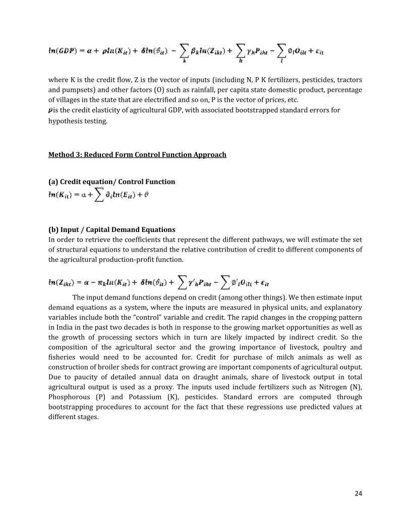
where K is the credit flow, Z is the vector of inputs (including N, P K fertilizers, pesticides, tractors

and pumpsets) and other factors (O) such as rainfall, per capita state domestic product, percentage

of villages in the state that are electrified and so on, P is the vector of prices, etc.

is the credit elasticity of agricultural GDP, with associated bootstrapped standard errors for

hypothesis testing.

Method 3: Reduced Form Control Function Approach

(a) Credit equation/ Control Function

(b) Input / Capital Demand Equations

In order to retrieve the coefficients that represent the different pathways, we will estimate the set

of structural equations to understand the relative contribution of credit to different components of

the agricultural production-profit function.

The input demand functions depend on credit (among other things). We then estimate input

demand equations as a system, where the inputs are measured in physical units, and explanatory

variables include both the “control” variable and credit. The rapid changes in the cropping pattern

in India in the past two decades is both in response to the growing market opportunities as well as

the growth of processing sectors which in turn are likely impacted by indirect credit. So the

composition of the agricultural sector and the growing importance of livestock, poultry and

fisheries would need to be accounted for. Credit for purchase of milch animals as well as

construction of broiler sheds for contract growing are important components of agricultural output.

Due to paucity of detailed annual data on draught animals, share of livestock output in total

agricultural output is used as a proxy. The inputs used include fertilizers such as Nitrogen (N),

Phosphorous (P) and Potassium (K), pesticides. Standard errors are computed through

bootstrapping procedures to account for the fact that these regressions use predicted values at

different stages.

25

(c) Outcome function

We then estimate the function explaining agricultural GDP in monetary terms as a hybrid profit

function. Compute the total impact of credit as the sum of the impacts on inputs weighted by the

impact of the input in question on agricultural GDP.

(d) Credit Elasticity of Agricultural GDP

The impact of credit on agricultural GDP can then be derived as the sum of the contribution of

credit to the use of specific inputs, capital or the cropping pattern, weighted by the contribution of

these to the total value of agricultural production. Standard errors reflect bootstrapped estimates.

26

APPENDIX 3: Data and Sources

Variable name Variable label (units) Mean Min Max Source

agelectariff Power tariff to agriculture

(paise/kWh)

80.72 0 512.88 Central Electricity Authority

EPWRF time series

animalhoursha Animal (hours/ha) 57.42 1.15 241.16 Ministry of Agriculture, Cost of

Cultivation Studies

areanonfoodtot

al

Total area unde nonfood crops

(`000 hectares)

2905.47 1 52398.00 Ministry of Agriculture

cagalliedtotal Total capital expenditure on

agriculture and allied services.

13384.02 -

67499

541032.00 State Finances : A Study of

Budgets, RBI

cladvecoservtot

al

Total capital expenditure on

economic services.

64155.42 -

18091

1881901.00 State Finances : A Study of

Budgets, RBI

commercial Number of commercial bank

branches

4165.49 7 101261.00 CMIE

egg_prod Production(in Lakhs) 12404.66 1 321068.00 Ministry of Agriculture,

Agricultural Statistics at a

Glance

fert_salepoint_t

otal

No. of Fertilizer Sale Points

(Total)

7835.36 0 72344.00 Ministry of Agriculture, Cost of

Cultivation Studies

gca Gross Cropped Area (`000 ha) 11606.41 2 195357.00 Ministry of Agriculture

gsdp_agri GSDP(in Rs. Lakh) 2943807.00 3943 127000000.00 Ministry of Agriculture

irrcanal Canal Irrigated area (`000 ha) 2178.10 0 17995.00 Ministry of Agriculture

irrtank Tank Irrigated area (`000 ha) 312.70 0 3343.00 Ministry of Agriculture

k Potassic fertilizers (`000 tonnes) 175.45 0.02 3632.40 Fertiliser Association of India

labhoursha Labour (hours/ha) wtd avg 568.69 211.6

6

1691.17 Ministry of Agriculture, Cost of

Cultivation Studies

machinersperha Machine (Rs./ha) 1417.22 0 6028.95 Ministry of Agriculture, Cost of

Cultivation Studies

milk_prod Production(in '000 MT) 2766.42 1 21031.00 Ministry of Agriculture,

Agricultural Statistics at a

Glance

n Nitrogenous fertilizers (`000

tonnes)

1092.02 0.6 17300.25 Fertiliser Association of India

nsa Net Sown Area (`000 ha) 8631.22 1 142960.00 Ministry of Agriculture

output_byprodu

ct

byproduct: Value of Output(Rs.

Lakhs)

176028.30 0 3222156.00 National Accounts Statistics

output_cereals Cereals: Value of Output(Rs.

Lakhs)


output_drugs drugs: Value of Output(Rs. Lakhs) 81793.53 0 1434137.00 National Accounts Statistics

output_fibres fibres: Value of Output(Rs. Lakhs) 94783.26 0 2756026.00 National Accounts Statistics

output_fish fish: Value of Output(Rs. Lakhs) 183344.90 19 3906563.00 National Accounts Statistics

output_fruits fruits: Value of Output(Rs. Lakhs) 607584.60 0 13800000.00 National Accounts Statistics

27

Variable name Variable label (units) Mean Min Max Source

output_livestock livestock: Value of Output(Rs.

Lakhs)


output_oilseeds oilseeds: Value of Output(Rs.

Lakhs)


output_othercro

ps

othercrops: Value of Output(Rs.

Lakhs)


output_pulses Pulses: Value of Output(Rs. Lakhs) 115964.70 0 2315486.00 National Accounts Statistics

output_spices spices: Value of Output(Rs. Lakhs) 79445.64 0 1838363.00 National Accounts Statistics

output_sugar sugar: Value of Output(Rs. Lakhs) 206510.30 0 3665781.00 National Accounts Statistics

p Phosphatic fertilizers (`000

tonnes)


pcsdpcurrent Per capita State Domestic Product 144345.00 3037 47200000.00 National Accounts Statistics

pcvillageselectri

c

Percentage of villages electrified 85.16 0 285.87 Central Electricity Authority

EPWRF time series

pesticide Pesticide Technical Grade

Consumption (MT)


pfertpest Price Index for Fertilisers and

Pesticides

100.50 70.42 148.50 RBI

pfodder Price Index for Fodder 114.77 63.17 245.64 RBI

pfoodarticles Price Index for Food Articles 121.15 67.9 215.20 RBI

pfuelpower Price Index for Fuel and Power 120.95 66.1 195.53 RBI

ptractor Price Index for Tractors 101.75 65.54 144.21 RBI

pumpset Pumpsets energized 835496.10 0 16300000.00 Central Electiricty Authority

ragrialliedtotal Government revenue expenditure

on agriculture and allied activities

132352.00 415 4339185.00 State Finances : A Study of

Budgets, RBI

rainavgann Rainfall Annual (mm) 995.41 0 2630.00 Ministry of Agriculture

seeds Certified seeds distributed (lakh

quintals)


total Total Disbursment (in Rs. lakh) 824263.20 0 46700000.00 DEAR, NABARD

tractorsale Sale of Tractors 28179.76 36 545109.00 Agricultural research data

book IASRI

tractorstock Stock of Tractors 312343.40 4629 4547080.00 CMIE

unskilledlabour

ers

Wage Index for unskilled

labourers

85.46 32.33 393.82 RBI

villelectric Percentage of villages electrified 85.16 0 285.87 EPWRF time series

wpi_all_avg Wholesale Price Index (Financial

Year averages)

102.51 63.58 152.33 RBI

wpi_allcalavg Wholesale Price Index (Calendar

Year averages)

97.05 58.28 164.93 RBI

Observations with missing values are excluded from the regression

28

APPENDIX 4 : Regression Results for SURE Model 3.

Variables (in deviation, log form) Fertilizers Pesticides

Both

Phases Phase 1 Phase 2

Both


b/t b/t b/t b/t b/t b/t

Credit 0.169 0.326* 0.058 0.510** 0.827 0.263

(1.88) (2.03) (0.51) (2.69) (1.54) (1.30)

"Error" from Control function 0.003 0.025 -0.103 0.077 -0.035 0.530

(0.05) (0.11) (-0.86) (0.46) (-0.05) (1.58)

Net Sown Area 0.632* 0.441 0.255 1.261 0.762 0.288

(2.01) (0.88) (0.50) (1.39) (0.57) (0.22)

Area under non-food Crops 0.000 0.000 0.000 -0.000 0.000 -0.000

(1.04) (0.25) (1.24) (-0.36) (1.51) (-1.50)

Fertilizer Sale points 0.000 0.000 0.000 0.000 0.000 -0.000

(0.73) (1.30) (0.27) (0.15) (0.93) (-0.50)

Index of Fertilizer/Pesticide prices -0.002 0.036* 0.021 -0.011 -0.006 -0.069

(-0.58) (1.96) (1.14) (-0.80) (-0.09) (-1.47)

Wholesale Price Index -0.002 0.015 0.002 -0.026* -0.079 -0.008

(-0.46) (0.92) (0.15) (-2.00) (-1.17) (-0.28)

Lagged Food Articles Price Index 0.006** -0.074 -0.001 0.016* 0.068 0.018

(2.74) (-1.83) (-0.13) (2.32) (0.45) (0.80)

(LAGGED) SHARE OF TOTAL VALUE OF AGRICULTURAL OUTPUT

Fibres 0.003*** 0.002 0.002* -0.002 -0.002 -0.002

(3.71) (1.52) (2.06) (-0.73) (-0.36) (-0.66)

Spices -0.000 -0.001 0.000 0.001 0.008 -0.004

(-0.09) (-0.53) (0.23) (0.21) (0.75) (-0.69)

Cereals 0.000 0.001 -0.000 -0.001 -0.002 0.001

(0.69) (1.06) (-0.27) (-0.67) (-0.64) (0.47)

Fruits -0.000 -0.000 0.000 0.000 -0.001 0.000

(-0.04) (-0.28) (0.12) (0.03) (-0.34) (0.14)

Oilseeds 0.000 -0.000 0.000 0.001 0.003 -0.004

(0.53) (-0.23) (0.49) (0.42) (0.58) (-1.21)

Pulses 0.001 -0.000 0.000 -0.000 -0.001 -0.007

(0.72) (-0.03) (0.06) (-0.17) (-0.27) (-1.28)

Sugar -0.000 0.000 -0.000 -0.001 0.001 -0.001

(-0.37) (0.03) (-0.01) (-0.53) (0.25) (-0.21)

Per Capita State Domestic Product -0.000 -0.000 0.000 -0.000 0.000 -0.000

(-0.32) (-0.46) (0.36) (-0.07) (0.19) (-0.39)

Annual Average Rainfall 0.016 0.024 0.004 -0.165 -0.041 0.078

(0.36) (0.26) (0.06) (-1.09) (-0.09) (0.32)

Constant -0.182 2.855 -2.394 2.154* 1.419 6.199

(-0.49) (1.92) (-1.38) (1.98) (0.27) (1.60)

b refers to coefficient and t refers to t value (in parenthesis)

29

APPENDIX 4 (Continued)

Variables (in deviation, log form) Animal hours per ha Machine expenses per hectare Labour hours per hectare

Both


Both


Both


b/t b/t b/t b/t b/t b/t b/t b/t b/t

Credit 0.176 -0.070 -0.038 -0.671* -1.125 -0.172 -0.200* -0.282 -0.157

(0.83) (-0.21) (-0.09) (-2.02) (-1.34) (-0.77) (-2.36) (-1.47) (-1.07)

"Error" from Control function 0.147 0.090 0.231 -0.633 -0.062 -0.297 -0.078 -0.052 0.036

(0.62) (0.19) (0.46) (-0.94) (-0.05) (-1.09) (-1.01) (-0.21) (0.24)

Net Sown Area 0.865 0.249 2.563 0.679 2.608 -0.259 0.252 0.442 -0.116

(1.46) (0.26) (1.45) (0.72) (1.06) (-0.22) (1.15) (0.87) (-0.18)

Area under non-food Crops 0.000 -0.000 0.000 -0.000 0.000 -0.000 0.000 -0.000 0.000

(0.82) (-0.68) (0.31) (-0.05) (0.47) (-0.43) (0.54) (-0.70) (0.53)

Fertilizer Sale points 0.000 0.000 0.000 -0.000 -0.000 0.000 -0.000 -0.000 -0.000

(0.68) (0.64) (0.34) (-0.65) (-1.40) (0.59) (-1.67) (-0.83) (-1.11)

Index of Fertilizer/Pesticide prices -0.020 -0.041 0.048 0.032 0.021 0.030 -0.007 -0.014 0.012

(-1.19) (-0.79) (0.58) (1.82) (0.20) (0.74) (-1.44) (-0.53) (0.46)

Wholesale Price Index 0.007 -0.020 0.045 0.056* 0.072 -0.005 0.011* 0.005 0.019

(0.52) (-0.55) (0.97) (2.43) (0.76) (-0.25) (2.03) (0.31) (1.18)

Lagged Food Articles Price Index -0.007 0.053 -0.036 -0.030** 0.015 0.004 -0.001 0.019 -0.012

(-0.93) (0.51) (-1.12) (-2.96) (0.07) (0.28) (-0.30) (0.41) (-1.20)


Fibres 0.001 -0.003 0.000 -0.003 -0.004 0.001 0.002* -0.000 0.005***

(0.43) (-0.75) (0.01) (-1.34) (-0.47) (0.38) (2.17) (-0.11) (3.98)

Spices 0.001 -0.006 0.007 -0.013 -0.028 -0.002 -0.002 -0.004 0.001

(0.23) (-1.05) (0.63) (-1.31) (-1.20) (-0.47) (-1.27) (-1.32) (0.18)

Cereals 0.003* 0.002 0.006 0.002 0.008 -0.002 0.001* 0.001 0.002*

(2.46) (1.01) (1.85) (1.24) (1.77) (-1.25) (2.19) (0.92) (2.13)

Fruits 0.002 0.001 0.004 -0.002 0.001 -0.003 0.001 0.000 0.001

(1.31) (0.45) (0.98) (-0.88) (0.29) (-1.12) (1.15) (0.35) (0.75)

Oilseeds -0.000 0.002 -0.004 0.001 -0.000 0.002 0.001 0.001 0.000

(-0.08) (0.75) (-0.80) (0.54) (-0.01) (0.75) (0.85) (0.67) (0.19)

Pulses -0.004 -0.002 -0.009 0.006 0.009 0.003 -0.003*** -0.002 -0.003

(-1.26) (-0.50) (-1.15) (1.79) (1.12) (0.69) (-3.41) (-1.01) (-1.16)

Sugar 0.003 -0.000 0.009 0.000 -0.004 -0.002 0.001 -0.000 0.002

(1.09) (-0.02) (1.81) (0.15) (-0.41) (-0.67) (1.33) (-0.04) (1.03)

30

Variables (in deviation, log form) Animal hours per ha Machine expenses per hectare Labour hours per hectare

Both


Both


Both


b/t b/t b/t b/t b/t b/t b/t b/t b/t

Per Capita State Domestic Product -0.000 0.000 -0.000* -0.000 -0.000 0.000 -0.000 -0.000 -0.000

(-1.21) (0.75) (-2.06) (-0.46) (-0.86) (0.64) (-0.98) (-0.33) (-0.75)

Annual Average Rainfall -0.153 -0.104 -0.039 -0.108 -0.518 -0.135 0.110 0.182 0.056

(-0.70) (-0.49) (-0.10) (-0.49) (-0.68) (-0.84) (1.41) (1.02) (0.57)

Constant 1.847 0.421 -6.334 -6.280** -11.712 -2.720 -0.363 -1.401 -2.127

(1.33) (0.12) (-0.95) (-3.23) (-1.72) (-0.84) (-0.74) (-0.87) (-1.04)

b refers to coefficient and t refers to t-value (in parenthesis)

31

APPENDIX TABLE 4 (Continued)

Variables (in deviation, log form) Tractor sale Pumpsets

Both


Both


b/t b/t b/t b/t b/t b/t

Credit 1.079*** 0.096 1.671** -0.842 0.038 -0.832

(3.32) (0.18) (3.11) (-1.52) (0.03) (-0.82)

"Error" from Control function -0.025 0.347 0.040 -0.067 -1.084 -0.557

(-0.07) (0.45) (0.08) (-0.08) (-0.62) (-0.48)

Net Sown Area -0.094 0.297 0.562 0.778 -1.698 5.586

(-0.13) (0.20) (0.26) (0.38) (-0.56) (1.04)

Area under non-food Crops 0.000 -0.000 0.000 -0.000 -0.000 -0.000

(0.72) (-0.62) (0.92) (-0.36) (-0.37) (-0.23)

Index of Fertilizer/Pesticide prices

0.048 0.456 0.009

(0.83) (1.58) (0.05)

Wholesale Price Index -0.054** -0.013 -0.000 0.007 -0.477 0.041

(-2.85) (-0.09) (-0.00) (0.15) (-1.74) (0.18)

Lagged Food Articles Price Index 0.012 -0.129 0.040 -0.029 0.310 -0.040

(1.33) (-0.70) (0.60) (-1.13) (0.79) (-0.31)

Tractor price index -0.007 0.133 -0.109

(-0.33) (0.92) (-1.74)

Unskilled workers wage index 0.005 0.013 0.004 -0.002 0.025 -0.010

(1.02) (0.89) (0.31) (-0.16) (0.76) (-0.37)

Fule and Power price index 0.004 0.010 -0.055 -0.001 -0.076 0.007

(1.56) (0.94) (-0.87) (-0.16) (-1.91) (0.09)


Fibres -0.002 -0.002 -0.004 -0.002 0.004 -0.005

(-0.59) (-0.30) (-0.59) (-0.44) (0.40) (-0.38)

Spices 0.009 0.013 0.004 -0.009 -0.003 -0.016

(1.51) (1.03) (0.32) (-0.51) (-0.14) (-0.48)

Cereals -0.001 -0.002 -0.003 -0.001 0.001 -0.003

(-1.01) (-0.69) (-0.82) (-0.23) (0.16) (-0.47)

Fruits 0.000 0.003 -0.003 -0.003 -0.007 -0.000

(0.21) (1.11) (-0.72) (-0.76) (-0.84) (-0.00)

Oilseeds 0.001 -0.000 -0.003 -0.001 -0.002 0.001

(0.66) (-0.10) (-0.66) (-0.32) (-0.44) (0.05)

Pulses 0.004 0.005 -0.000 -0.008 -0.002 -0.005

(1.45) (0.74) (-0.02) (-1.17) (-0.20) (-0.22)

Sugar -0.008* -0.009 -0.012 0.015* 0.015 0.017

(-2.54) (-1.24) (-1.87) (2.39) (1.18) (1.31)

Per Capita State Domestic Product 0.000* 0.000 0.000 0.000** 0.000* 0.000

(2.02) (0.08) (1.18) (3.03) (2.03) (1.32)

Annual Average Rainfall 0.226 0.195 -0.217 -0.393 0.529 -0.484

(1.21) (0.39) (-0.45) (-0.95) (0.63) (-0.64)

Constant 4.835* 1.170 12.919* -1.789 -20.078 -1.878

(2.54) (0.11) (2.17) (-0.48) (-1.19) (-0.12)

32

APPENDIX 5: Results for Agricultural GDP as part of SURE Model 3

Variable (in log devation form) Both Phases Phase 1 Phase 2

b/t b/t b/t

Credit 0.083 -0.095 0.133

(1.00) (-0.39) (0.77)

"Error" from Control Function -0.028 -0.130 -0.042

(-0.42) (-0.37) (-0.37)

Milk production 0.000 0.000 -0.000

(0.52) (0.95) (-0.18)

Egg production 0.000 0.000 0.000

(1.43) (0.47) (0.10)

Gross cropped area 0.193 0.186 -0.124

(0.92) (0.44) (-0.18)

Land irrigated by canals 0.010 0.044 -0.017

(0.41) (0.65) (-0.21)

Land irrigated by tanks 0.011 0.002 0.030

(0.36) (0.03) (0.32)

Area under Non-food crops -0.000 -0.000 0.000

(-0.63) (-0.07) (0.11)

Pesticide 0.010 0.032 -0.045

(0.31) (0.32) (-0.43)

Fertilizers (N, P and K) 0.492** 0.745* 0.184

(2.82) (2.42) (0.66)

Tractors -0.073 -0.005 -0.101

(-1.32) (-0.04) (-0.69)

Pumpsets -0.210 0.033 -0.074

(-1.16) (0.07) (-0.18)

Labour hours per hectare 0.265** 0.216 0.350

(3.12) (0.99) (1.95)

Aimal hours per hectare -0.040 -0.043 -0.017

(-1.20) (-0.32) (-0.26)

Machine (Rs. Per hectare) -0.001 0.014 -0.003

(-0.02) (0.14) (-0.02)

Lagged unskilled wage index 0.001 -0.000 0.002

(0.96) (-0.09) (0.49)

Average Annual Rainfall -0.016 -0.032 -0.025

(-0.33) (-0.24) (-0.26)

Lagged Fertilizer and Pesticide price index 0.020** 0.071 0.161

(3.28) (0.99) (0.58)

Lagged Fodder price index 0.002 0.003 -0.019

(1.42) (1.23) (-0.52)

Lagged tractor price index -0.006 -0.019 0.011

(-0.74) (-0.56) (0.24)

Lagged Fuel and power price index -0.003** -0.012 -0.011

(-2.69) (-0.77) (-0.58)

33

Variable (in log devation form) Both Phases Phase 1 Phase 2

b/t b/t b/t

Wholesale Price Index -0.006 -0.015 -0.028

(-0.89) (-0.55) (-0.50)

Capital expenditure on economic services -0.009 -0.019 -0.005

(-0.80) (-0.64) (-0.25)

Capital expenditure on Agriculture and allied services 0.000 -0.001 0.001

(0.06) (-0.14) (0.06)

Revenue expenditure on agriculture and allied

services 0.076 -0.052 0.056

(0.87) (-0.31) (0.49)

Percentage of villages electrified -0.000 0.008 -0.002

(-0.03) (0.78) (-0.34)

Constant -0.105 0.000 -0.488

(-0.80) (.) (-0.37)

N 121.00 59.00 62.00

R-squared 0.74 0.47 0.69

BIC 603.77 411.02 324.76

AIC 170.42 91.08 -4.948

b refers to coefficient and t refers to t-value (in parenthesis)

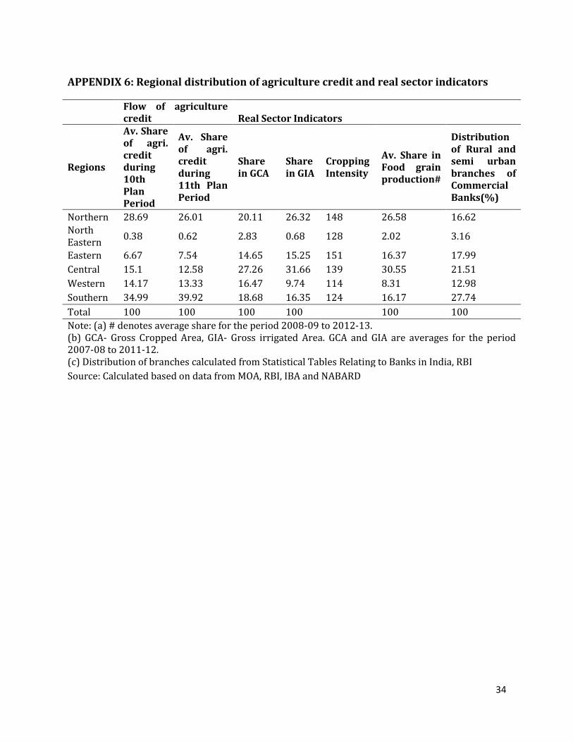
34

APPENDIX 6: Regional distribution of agriculture credit and real sector indicators

Flow of agriculture credit Real Sector Indicators

Regions

Av. Share of agri. credit during 10th Plan Period

Av. Share of agri. credit during 11th Plan Period

Share in GCA

Share in GIA

Cropping Intensity

Av. Share in Food grain production#

Distribution of Rural and semi urban branches of Commercial Banks(%)

Northern 28.69 26.01 20.11 26.32 148 26.58 16.62

North Eastern

0.38 0.62 2.83 0.68 128 2.02 3.16

Eastern 6.67 7.54 14.65 15.25 151 16.37 17.99

Central 15.1 12.58 27.26 31.66 139 30.55 21.51

Western 14.17 13.33 16.47 9.74 114 8.31 12.98

Southern 34.99 39.92 18.68 16.35 124 16.17 27.74

Total 100 100 100 100 100 100

Note: (a) # denotes average share for the period 2008-09 to 2012-13. (b) GCA- Gross Cropped Area, GIA- Gross irrigated Area. GCA and GIA are averages for the period 2007-08 to 2011-12. (c) Distribution of branches calculated from Statistical Tables Relating to Banks in India, RBI

Source: Calculated based on data from MOA, RBI, IBA and NABARD

Documents

The Productivity of Agricultural Credit in India · 2015-01-23 · The Productivity of Agricultural Credit in India ... in response to the persistent problem of indebtedness and to