NISTIR 5703

The NISTATM Network Simulator

Operation and Programming

Version 1.0

Nada GolmieAlfred KoenigDavid Su

U.S. DEPARTMENT OF COMMERCETechnology AdministrationNational Institute of Standards and TechnologyComputer Systems LaboratoryAdvanced Systems DivisionGaithersburg, MD 20899

August 1995

TABLE OF CONTENTS

Introduction . . . . . . . . . . . . . . . . . . . . . . . . . . . . . . . . . . . . . . . . . . . . . . . . . . . . 1Purpose . . . . . . . . . . . . . . . . . . . . . . . . . . . . . . . . . . . . . . . . . . . . . . . . . . . . 1Terminology in this Manual. . . . . . . . . . . . . . . . . . . . . . . . . . . . . . . . . . . . . . 2

PART 1. User’s Manual . . . . . . . . . . . . . . . . . . . . . . . . . . . . . . . . . . . . . . . . . 31.1 Objectives and Overview. . . . . . . . . . . . . . . . . . . . . . . . . . . . . . . . . . . . . 31.2 Component Descriptions. . . . . . . . . . . . . . . . . . . . . . . . . . . . . . . . . . . . . 5

1.2.1 ATM Switch.. . . . . . . . . . . . . . . . . . . . . . . . . . . . . . . . . . . . . . . 51.2.2 Broadband Terminal Equipment (B-TE).. . . . . . . . . . . . . . . . . . . . 51.2.3 ATM Application. . . . . . . . . . . . . . . . . . . . . . . . . . . . . . . . . . . . 51.2.4 Physical Link. . . . . . . . . . . . . . . . . . . . . . . . . . . . . . . . . . . . . . . 5

1.3 Executing the Program. . . . . . . . . . . . . . . . . . . . . . . . . . . . . . . . . . . . . . 61.4 The Display . . . . . . . . . . . . . . . . . . . . . . . . . . . . . . . . . . . . . . . . . . . . . . 7

1.4.1 The Network Window . . . . . . . . . . . . . . . . . . . . . . . . . . . . . . . . 71.4.2 The Text Window . . . . . . . . . . . . . . . . . . . . . . . . . . . . . . . . . . . 71.4.3 The Control Panel. . . . . . . . . . . . . . . . . . . . . . . . . . . . . . . . . . . 7

1.4.3.1 Analog Clock.. . . . . . . . . . . . . . . . . . . . . . . . . . . . . . . . 81.4.3.2 Digital Clock. . . . . . . . . . . . . . . . . . . . . . . . . . . . . . . . . 81.4.3.3 Control Buttons.. . . . . . . . . . . . . . . . . . . . . . . . . . . . . . 9

1.5 Operating the Simulator. . . . . . . . . . . . . . . . . . . . . . . . . . . . . . . . . . . . . . 111.5.1 Loading a Network Configuration. . . . . . . . . . . . . . . . . . . . . . . . 111.5.2 Creating a Network Configuration. . . . . . . . . . . . . . . . . . . . . . . . 11

1.5.2.1 Creating Components.. . . . . . . . . . . . . . . . . . . . . . . . . . 111.5.2.3 Linking Components.. . . . . . . . . . . . . . . . . . . . . . . . . . . 121.5.2.3 Creating Routes.. . . . . . . . . . . . . . . . . . . . . . . . . . . . . . 12

1.6 Operational Features. . . . . . . . . . . . . . . . . . . . . . . . . . . . . . . . . . . . . . . . 131.6.1 Displaying Information about the Network. . . . . . . . . . . . . . . . . . 13

1.6.1.1 Component Information Windows.. . . . . . . . . . . . . . . . . 131.6.1.2 Meters.. . . . . . . . . . . . . . . . . . . . . . . . . . . . . . . . . . . . . 141.6.1.3 Logging Data.. . . . . . . . . . . . . . . . . . . . . . . . . . . . . . . . 151.6.1.4 Log File Format.. . . . . . . . . . . . . . . . . . . . . . . . . . . . . . 15

1.6.2 Making Modifications. . . . . . . . . . . . . . . . . . . . . . . . . . . . . . . . . 161.6.2.1 Modifying Components.. . . . . . . . . . . . . . . . . . . . . . . . . 161.6.2.2 Deleting Components.. . . . . . . . . . . . . . . . . . . . . . . . . . 16

1.6.3 Manipulating the Network Display. . . . . . . . . . . . . . . . . . . . . . . . 161.6.3.1 Raising/Lowering Windows.. . . . . . . . . . . . . . . . . . . . . . 161.6.3.2 Moving Windows.. . . . . . . . . . . . . . . . . . . . . . . . . . . . . 161.6.3.3 Resizing Windows.. . . . . . . . . . . . . . . . . . . . . . . . . . . . 171.6.3.4 Resizing Information Windows.. . . . . . . . . . . . . . . . . . . 17

1.6.4 Saving a Network Configuration. . . . . . . . . . . . . . . . . . . . . . . . . 17

i

1.6.5 Post Simulation Analysis using the Log File. . . . . . . . . . . . . . . . . 171.7 Simulator Concepts. . . . . . . . . . . . . . . . . . . . . . . . . . . . . . . . . . . . . . . . . 19

1.7.1 Simulation Clock. . . . . . . . . . . . . . . . . . . . . . . . . . . . . . . . . . . . 191.7.2 ATM Switch . . . . . . . . . . . . . . . . . . . . . . . . . . . . . . . . . . . . . . . 191.7.3 Broadband Terminal Equipment (B-TE). . . . . . . . . . . . . . . . . . . . 191.7.4 ATM Applications . . . . . . . . . . . . . . . . . . . . . . . . . . . . . . . . . . . 201.7.5 Link Components. . . . . . . . . . . . . . . . . . . . . . . . . . . . . . . . . . . . 20

PART 2. Programmer’s Guide . . . . . . . . . . . . . . . . . . . . . . . . . . . . . . . . . . . 212.1 Objectives and Overview. . . . . . . . . . . . . . . . . . . . . . . . . . . . . . . . . . . . . 212.2 Components. . . . . . . . . . . . . . . . . . . . . . . . . . . . . . . . . . . . . . . . . . . . . . 22

2.2.1 Classes and Types. . . . . . . . . . . . . . . . . . . . . . . . . . . . . . . . . . . 222.2.2 Component Data Structures. . . . . . . . . . . . . . . . . . . . . . . . . . . . . 232.2.3 Parameters. . . . . . . . . . . . . . . . . . . . . . . . . . . . . . . . . . . . . . . . . 232.2.4 Neighbors. . . . . . . . . . . . . . . . . . . . . . . . . . . . . . . . . . . . . . . . . 272.2.5 Relationship of Data Structures. . . . . . . . . . . . . . . . . . . . . . . . . . 282.2.6 Action Routines. . . . . . . . . . . . . . . . . . . . . . . . . . . . . . . . . . . . . 29

2.3 Events. . . . . . . . . . . . . . . . . . . . . . . . . . . . . . . . . . . . . . . . . . . . . . . . . . 312.3.1 Command Set (EV_CLASS_CMD). . . . . . . . . . . . . . . . . . . . . . . 312.3.2 Regular Events (EV_CLASS_EVENT). . . . . . . . . . . . . . . . . . . . 322.3.3 Private Events. . . . . . . . . . . . . . . . . . . . . . . . . . . . . . . . . . . . . . 332.3.4 The Event Manager. . . . . . . . . . . . . . . . . . . . . . . . . . . . . . . . . . 33

2.4 ATM Network-Related Issues. . . . . . . . . . . . . . . . . . . . . . . . . . . . . . . . . . 352.4.1 ATM Cell Definition . . . . . . . . . . . . . . . . . . . . . . . . . . . . . . . . . 352.4.2 Setting Up the ATM Virtual Channel. . . . . . . . . . . . . . . . . . . . . . 36

2.5 Tools. . . . . . . . . . . . . . . . . . . . . . . . . . . . . . . . . . . . . . . . . . . . . . . . . . . 372.5.1 Lists and Queues. . . . . . . . . . . . . . . . . . . . . . . . . . . . . . . . . . . . 372.5.2 Other Tools. . . . . . . . . . . . . . . . . . . . . . . . . . . . . . . . . . . . . . . . 392.5.3 Debugging. . . . . . . . . . . . . . . . . . . . . . . . . . . . . . . . . . . . . . . . . 39

2.6 Creating New Versions. . . . . . . . . . . . . . . . . . . . . . . . . . . . . . . . . . . . . . 41

APPENDIX A: Parameter Information . . . . . . . . . . . . . . . . . . . . . . . . . . . . . . . . . 43A.1 ATM Switches. . . . . . . . . . . . . . . . . . . . . . . . . . . . . . . . . . . . . . . . . . . . 43A.2 Broadband Terminal Equipment (B-TE). . . . . . . . . . . . . . . . . . . . . . . . . . 45A.3 ATM Applications . . . . . . . . . . . . . . . . . . . . . . . . . . . . . . . . . . . . . . . . . 46

Constant Bit Rate (CBR) Information Window. . . . . . . . . . . . . . . . . . . . 47Variable Bit Rate (VBR) (Poisson) Information Window. . . . . . . . . . . . . 47Variable Bit Rate (VBR) (Batch) Information Window. . . . . . . . . . . . . . 47Available Bit Rate (ABR) (Constant) Information Window. . . . . . . . . . . 48Available Bit Rate (ABR) (Poisson) Information Window. . . . . . . . . . . . 48Available Bit Rate (ABR) (Batch) Information Window. . . . . . . . . . . . . . 48TCP/IP Information Window . . . . . . . . . . . . . . . . . . . . . . . . . . . . . . . . 49

A.4 Link Components. . . . . . . . . . . . . . . . . . . . . . . . . . . . . . . . . . . . . . . . . . 51

ii

APPENDIX B: Meter Types . . . . . . . . . . . . . . . . . . . . . . . . . . . . . . . . . . . . . . . . . 53

APPENDIX C: Configuration File Formats . . . . . . . . . . . . . . . . . . . . . . . . . . . . . . 55C.1 Format of the SAVE file. . . . . . . . . . . . . . . . . . . . . . . . . . . . . . . . . . . . . 55C.2 Format of the SNAP File.. . . . . . . . . . . . . . . . . . . . . . . . . . . . . . . . . . . . 56

iii

The NIST ATM Network Simulator

Operation and Programming

Version 1.0

ABSTRACT

An Asynchronous Transfer Mode (ATM) network simulator has been developedto provide a means for researchers and network planners to analyze the behaviorof ATM networks without the expense of building a real network. The simulatoris a tool that gives the user an interactive modeling environment with a graphicaluser interface. With this tool the user may create different network topologies,control component parameters, measure network activity, and log data fromsimulation runs. Part 1 of this document is the user’s manual for the simulator;it includes instructions for creating network configurations, specifying componentparameters, manipulating the display, logging and saving measurements, and post-processing of data. Part 2 has been prepared as a guide for the user who wishesto modify the simulator software to accommodate network components notpreviously defined or to change the behavior of components already defined.

Introduction

The ATM Network Simulator was developed at the National Institute of Standards andTechnology (NIST) to provide a flexible testbed for studying and evaluating the performance ofATM networks. The simulator is a tool that gives the user an interactive modeling environmentwith a graphical user interface. NIST has developed this tool using both C language and the XWindow System running on a UNIX platform. This tool is based on a network simulatordeveloped at MIT1 that provides support for discrete event simulation techniques and has graphicuser interface (GUI) representation capabilities.

The ATM Network Simulator allows the user to create different network topologies, set theparameters of component operation, and save/load the different simulated configurations. Whilethe simulation is running, various instantaneous performance measures can be displayed ingraphical/text form on the screen or saved to files for subsequent analysis.

Purpose

The ATM network simulator is a tool to analyze the behavior of ATM networks without theexpense of building a real network. There are two major uses for the simulator: as a tool for

1A. Heybey, "The Network Simulator,"Laboratory of Computer Science, Massachusetts Institute of Technology,October 1989.

ATM network planning and as a tool for ATM protocol performance analysis. As a planningtool, a network planner can run the simulator with various network configurations and trafficloads to obtain statistics such as utilization of network links and throughput rates of virtualcircuits. It could be used to answer questions such as: where will be the bottlenecks in theplanned network, what is the effect of changing the speed of a link, will adding a new applicationcause congestion, etc. Statistics are reported directly to the screen or logged in a data file forfurther processing.

As a protocol analysis tool, a researcher or protocol designer could study the total system effectof a particular protocol. For example, one could investigate the effectiveness of various flowcontrol mechanisms for ATM networks and address such issues as: mechanisms for fairbandwidth allocation, protocol overhead, bandwidth utilization, etc. In order to conductexperiments, an investigator must first change or add additional codes to implement the protocolto be studied. The simulator is designed in such a way that modules simulating components ofan ATM network can be easily changed, added, or deleted. Activities can be recorded on a cellby cell basis for subsequent analysis.

Terminology in this Manual

The network to be simulated consists of severalcomponentssending messages to one another.The components available includeATM Switches, Broadband Terminal Equipment (B-TE), andATM Applications. Switches and B-TE components are interconnected withPhysical Links; aPhysical Link is also considered a component. The ATM Applications are logical entities thatrun on B-TE (hosts). The Applications may be considered as traffic generators that are capableof emulating variable or constant bit rate traffic sources. ATM Applications are connected toeach other over aroute that uses a selected list of adjacent components to form an end-to-endvirtual connection.

All components are characterized by one or moreparameters. Parameters fall into twocategories, input and output; both kinds are listed ininformation windowswhich appear next tothe applicable component when the user so desires. All input parameters may be specified bythe user at the time of component creation or they may be modified later. Network activity maybe observed by openingmeter windowsto display selected parameters. There are various typesof meter windows available and they can be placed anywhere on the screen. Parameterinformation may also belogged, i.e., stored on disk in a file namedsim_log.xxxxwherexxxx isthe process ID of the simulator.

2

PART 1. User’s Manual

1.1 Objectives and Overview

This part of the document provides information for the simulator user to create networktopologies using simulated ATM switches, terminal equipment, and physical links. The manualincludes instructions for display manipulation, component linking and routing, parameter setting,data logging, and post-simulation analyses.

The user may select from a variety of applications, the behavior of which will determine the kindof traffic generated for transmission through the network. The user may control the parametersassociated with these components, define the routes, and specify many details concerning thelogging and display of performance data. The primary user interface to the simulator is throughan X Windows display screen. The screen simultaneously displays the network configuration,a control panel for running the simulation, and parameter information. The display contains atext window for user prompts which also provides a place for parameter data entry. Outputparameter values may be be displayed in numerical form in "information windows" or asgraphical "meters." Output parameter values may also be tagged for logging to a file; the datalogging frequency is determined by the user.

3

4

1.2 Component Descriptions

The following are brief, general descriptions of the major building blocks of the simulated ATMNetwork. For more detailed functional descriptions, see1.7 Simulator Conceptsand 2.2Components. A complete list of input and output parameters available for each component canbe found inAppendix A.

1.2.1 ATM Switch. This is the component used to switch or route cells over several virtualchannel links. When a switch accepts an incoming cell from a Physical Link it looks in itsrouting table to determine which outgoing link should send it. If the outgoing link is busy, theswitch will queue the cells destined for that link and not send them until free cell slots areavailable for transmission. The user may specify the processing delay time, maximum outputqueue size, and queue size thresholds. The parameters that can be monitored for a switch includethe number of cells received, number of cells in an output queue, number of cells dropped, andthe status of congestion flags.

1.2.2 Broadband Terminal Equipment (B-TE). This is a component to simulate a broadbandISDN node, e.g., host computer, workstation, etc. A B-TE component has one or more ATMApplications on one side and a physical link on the other side. Cells received from theApplication side are forwarded to the physical link; if the link is busy the cells go into a queue.The user can specify the maximum output queue size. The parameters that can be monitored arethe number of cells in an output queue and the number of cells dropped.

1.2.3 ATM Application. This is a component to emulate the behavior of an ATM applicationat the end-point of a link. It can be considered as a traffic generator, either with a constant orvariable bit rate. The user specifies the bit rate for constant bit rate (CBR) applications. Forvariable bit rate (VBR) applications the user sets the burst length, interval between bursts, andthe mean rate. For lower priority traffic, the user may create an available bit rate (ABR)application. For all of the application types, the user sets the start time and the number ofmegabytes to be sent. Other application types that can be simulated include TCP/IP applications.

1.2.4 Physical Link. This component simulates the physical medium (copper wire or opticalfiber) on which cells are transmitted. The user may choose the link speed from a list of severaldifferent standard rates. The user also specifies the length of the link. The output parameterreported by the simulator is link utilization in terms of bit rate (Mbits/s).

5

1.3 Executing the Program

To execute the ATM Network Simulator, the following is typed at the command line :

sim [-x] [-s seed] [configfile [stoptime]]

where:

-x Used for running the simulator in background mode. With this option thesimulator will not use X Windows; it will run on a machine that does not have XWindows. When using this option aconfigfile must be specified, otherwise thesimulator will have no network to simulate and will produce no meaningfulresults. Also, theconfigfile specified should be a "snapshot" that has someparameters logged to disk so that the simulator run produces some results.

-s Allows the user to specify the seed for the random number generator. If thisoption is omitted the current time (in UNIX format) is used as the seed. The seedactually used is printed at the beginning of each simulator run, and is saved as acomment in any log files produced by the simulator. Specifying a particular seedis useful if identical results are expected from successive simulator runs.

configfile A file describing the configuration of the network to simulate. Such a file isproduced by the SAVE and SNAP commands in the simulator.

stoptime Length of time (in microseconds of simulated time) for the simulator to run. Mostuseful when running non-interactively (with the-x option). When the simulatorstops, it will automatically produce a "snap" file of its current state.

6

1.4 The Display

The display is composed of three major parts:

· A network window to display ATM network configurations. This window is used bothwhile creating the configurations and to show network activity while the simulation isrunning.

· A text window for messages that will prompt the user, and to provide a place for the userto input text or parameter values.

· A control panel that consists of a clock and several control buttons, such as START,QUIT, etc..

1.4.1 The Network Window

Figure 1 is an example of the simulator screen seen by the user once a network configuration hasbeen created. The entire area not otherwise occupied by clock and control buttons is the NetworkWindow. If the program is started with noconfigfile this area is blank. The network isrepresented as a collection of components connected to each other in the desired configurations.ATM switches and broadband terminals (B-TEs) are represented by rectangular boxes while ATMApplications are represented by ellipses; both shapes contain the name of the component. ATMswitches and B-TEs are interconnected by Physical Links. The Links are also consideredcomponents and are identified by name, but they are represented on the figure by straight lines.The connection between a B-TE and an ATM Application is also represented by a line but is notconsidered a component, i.e., it is not a physical entity and has no associated parameters.

Other information (not shown on the figure) is displayed in the Network Window as required.When creating or modifying a component an information window appears beside its symbol,displaying the component’s parameters. When a virtual connection is established between ATMapplications a dotted line appears denoting the path of the information flow. When a simulationis running, one or more meters may appear on the screen to display information about selectedparameters.

1.4.2 The Text Window

The text window appears as a bar at the bottom of the screen. The text window allows theprogram to present various messages to the user. In addition, any keyboard input is displayedin the text window. The cursor does not need to be in the text window when enteringinformation with the keyboard. When entering information using the keyboard, pressing "Return"without entering any text will tell the program to accept a default value or to abort that operation.

1.4.3 The Control Panel

7

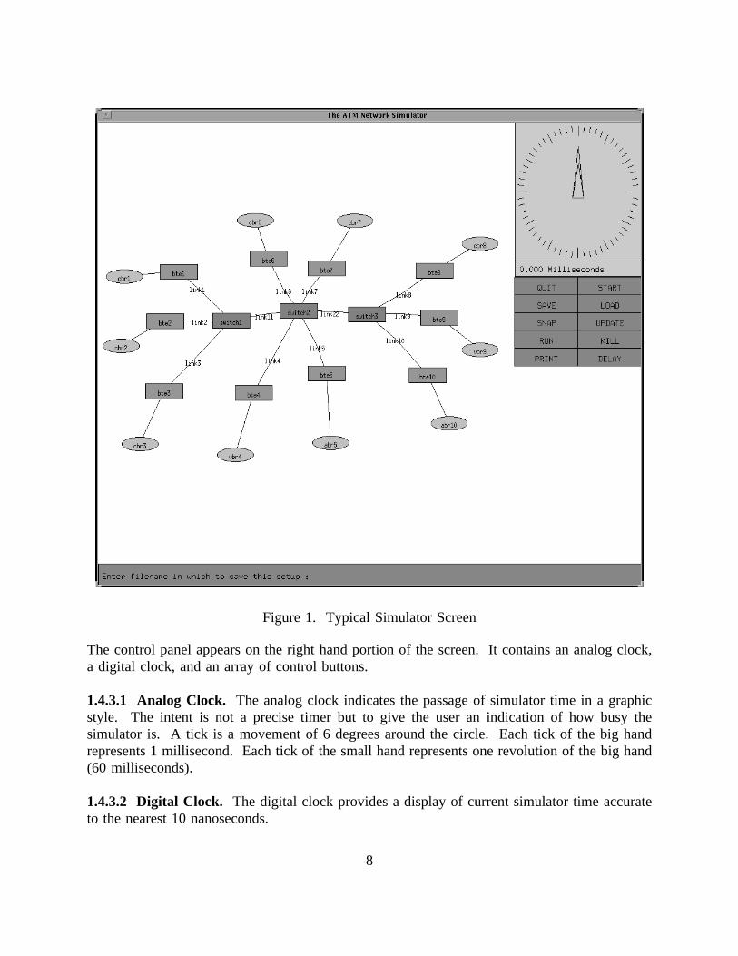
The control panel appears on the right hand portion of the screen. It contains an analog clock,

Figure 1. Typical Simulator Screen

a digital clock, and an array of control buttons.

1.4.3.1 Analog Clock. The analog clock indicates the passage of simulator time in a graphicstyle. The intent is not a precise timer but to give the user an indication of how busy thesimulator is. A tick is a movement of 6 degrees around the circle. Each tick of the big handrepresents 1 millisecond. Each tick of the small hand represents one revolution of the big hand(60 milliseconds).

1.4.3.2 Digital Clock. The digital clock provides a display of current simulator time accurateto the nearest 10 nanoseconds.

8

1.4.3.3 Control Buttons. The following is a description of the function of each control button.All of the functions are initiated by clicking with themiddle mouse button.

START Clicking on this button will start the simulation with simulated timeinitialized to zero. The simulation can be restarted as many times as theuser wishes; each click on the button will initialize the simulation.

PAUSE/RUN This button toggles between two modes. When the simulation is runningthe word PAUSE will be displayed. Clicking on the button will then stopall activity with all parameter and time information held in place. Withthe simulation stopped, the button label will change to RUN; clicking onit will cause the simulation to resume running with current settings.

DELAY This button allows the user to slow down the simulation by setting a delaybetween each event firing. The text window will appear asking for thedesired delay (in microseconds).

UPDATE Clicking on this button will toggle screen updating on or off. Thesimulation will run faster with screen updating turned off. The clock willcontinue to be displayed with updating turned off. Clicking on acomponent while updating is off will cause the parameter window for thatcomponent to appear with current data. Clicking on the component asecond time will make the window disappear.

KILL This button may be used to stop a simulation in progress or to eliminatecomponents. Clicking on the KILL button while a simulation is inprogress stops all activity. If a simulation is not running, clicking on acomponent after KILL has been clicked will delete that component. Ineither case, the QUIT button must be used to leave the KILL mode.

LOAD This button allows the user to load a network configuration. The textwindow appears asking for the name of the file to be loaded. Note thatthis erases whatever configuration was being displayed on the screen at thetime.

SAVE The SAVE control button allows the user to save the present configurationin a specially formatted text file which is readable by the simulator atLOAD time. The text window appears asking for a filename under whichto save the configuration. Present values of the components’ parametersare notsaved.

SNAP This is similar to SAVE, but in addition it saves the present arrangementof meters and information windows on the display. The text window

9

appears asking for a filename under which to save the configuration.Present values of the components’ parameters are saved.

PRINT Prints out the network topology into a postscript file.

QUIT This is the normal exit from the simulator program. Note that clicking onthe QUIT button while in KILL mode merely causes an exit from thatmode; it does notcause an exit from the program.

10

1.5 Operating the Simulator

1.5.1 Loading a Network Configuration

There are three ways to specify a network configuration for the program to simulate.

1. Specify the name of aconfigfile describing the network on the command line. Thisnetwork will be automatically loaded when the programs begins.

2. Use the LOAD command while in the simulator program. This is accomplished byclicking on the LOAD control button; a prompt will then appear in the text windowasking for a file name. After the user enters the name of the file, the networkconfiguration is loaded. Note that this erases whatever configuration was being displayedon the screen at the time.

3. Create a network while in the simulator program using the tools the program provides.Using this process, the user decides on the appropriate components, their characteristicsand interconnections.

1.5.2 Creating a Network Configuration

The process of creating a network for simulation starts with the creation of components.

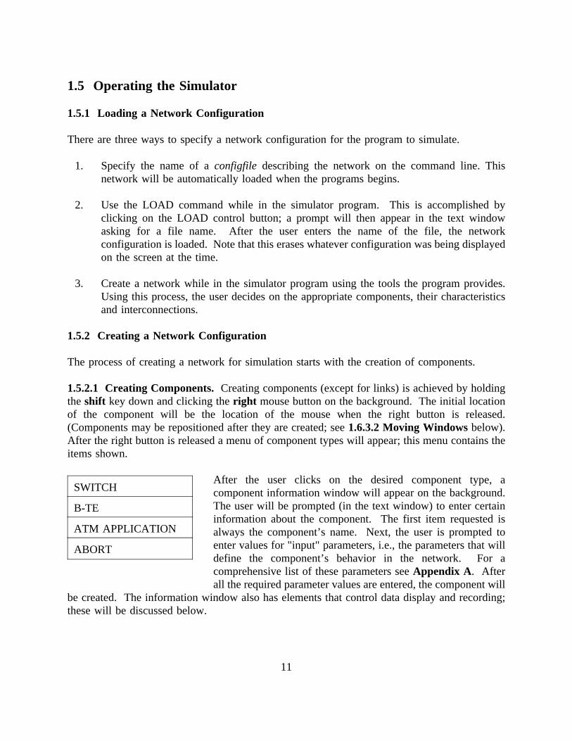
1.5.2.1 Creating Components.Creating components (except for links) is achieved by holdingtheshift key down and clicking theright mouse button on the background. The initial locationof the component will be the location of the mouse when the right button is released.(Components may be repositioned after they are created; see1.6.3.2 Moving Windowsbelow).After the right button is released a menu of component types will appear; this menu contains theitems shown.

After the user clicks on the desired component type, aSWITCH

B-TE

ATM APPLICATION

ABORT

component information window will appear on the background.The user will be prompted (in the text window) to enter certaininformation about the component. The first item requested isalways the component’s name. Next, the user is prompted toenter values for "input" parameters, i.e., the parameters that willdefine the component’s behavior in the network. For acomprehensive list of these parameters seeAppendix A. Afterall the required parameter values are entered, the component will

be created. The information window also has elements that control data display and recording;these will be discussed below.

11

1.5.2.3 Linking Components. After the ATM switches and B-TE components have beencreated they are connected into a network by creating physical links. A physical link is alsoconsidered to be a network component and has a name and parameters associated with it. A linkmay connect any two ATM switches or one switch and one B-TE. The procedure for creatinga link is as follows:

Select the first component to be linked by clicking on it with themiddle mouse buttonwhile holding down theshift key.

Select the second component to be linked by the same method. At this point a line willappear and the physical link component will be created. As with other components, aninformation window will appear and the user will be prompted to enter a name and someinput parameters.

To complete the linking process the ATM Application components must be connected to the B-TE components. The process is like creating the physical link (shift, click middle button oncomponent) but in this case only a line linking the components will appear, no informationwindow. This is because this type of connection is not considered a component.

1.5.2.3 Creating Routes.A Route is an ATM Permanent Virtual Connection, a path over whichthe cells travel through the network. In the simulator, a Route is a list of adjacent componentsbeginning and ending with ATM Applications. To create a Route, hold theshift key down andclick the left mouse button on each component in the route. A message will appear briefly inthe text window after each click to affirm (or reject) the addition of the component to the route.The first and last components in this process must be ATM Applications. When the user clickson the final Application on the path, the route is created. Only one route going out of an ATMApplication is assumed, although multiple routes may be coming in.

Performing a shift/left-click on anything other than a component aborts route creation. However,any other commands or button clicks that are not shift/left-clicks can take place at any time inthe route creation process. If the user attempts to include a component in the route which cannotbe included (perhaps because it is not a neighbor) it will not be included, but the route creationprocess will not be aborted. To abort an incomplete route creation process and start over,shift/left-click twice on the window background.

Once routes have been created they cannot be deleted. All desired routes should be created atone session, i.e., do not try to add routes to a loaded file that has been previously configured andcontains routes.

CAUTION: Any attempt to start or run a simulation before routes have been created will causea program crash.

12

1.6 Operational Features

The simulator provides several features which may be used to enhance the display of information,modify the network that was created, save existing configurations, and log data from thesimulation runs.

1.6.1 Displaying Information about the Network

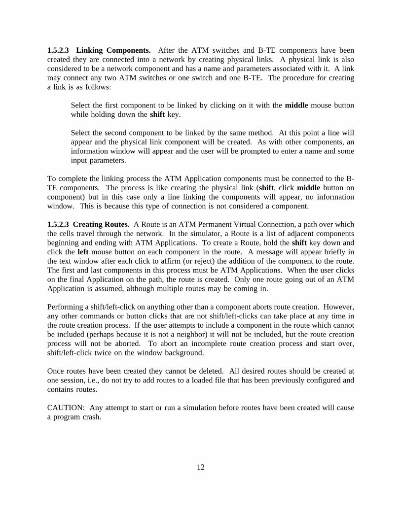
1.6.1.1 Component Information Windows. These are the same windows that appear when acomponent is created. They are used during the process of setting values of input parameters butmay also be used to modify those values, display output parameter values, and to control datalogging. The figure below is an example of an information window. The first line shows thecomponent name, the second line an input parameter. The two shaded blocks are outputparameters with current parameter values displayed. (Note: This shading does not appear on thescreen).

To bring the information window onto the screen, click themiddle mouse button on the

switch1

Max. Output Queue Size (-1=inf): -1

Link 1 output queue has 25 cells

Number of cells dropped on route = 0

component’s symbol; a window similar to the one above will appear. To the left of eachparameter’s information line are two small boxes. Clicking themiddle mouse button on theleft-hand box toggles a meter display on and off for that parameter; clicking on the right-handbox toggles data logging on and off for the parameter. The box will become white when itsfunction is turned on and revert back to its background color when it is toggled off. Theexample above shows a meter created for "Link 1 output ..." and data logging selected for"Number of cells dropped ..." Both box types are valid only for output parameters; clicking oneither box for any other parameter will have no effect.

When defining a component for the first time, a prompt will appear in the text windowautomatically, asking for the required information. Each entry is terminated by a RETURN. Noother action is possible until all requested information has been entered. To modify a parameterat any other time, click the middle mouse button on the desired line. Once again the prompt willappear in the text window and the value may be entered, terminated by a RETURN. A RETURNwith no entry will accept the current value.

To remove the information window from the screen, click the middle button on the component’ssymbol, and the information window will disappear.

13

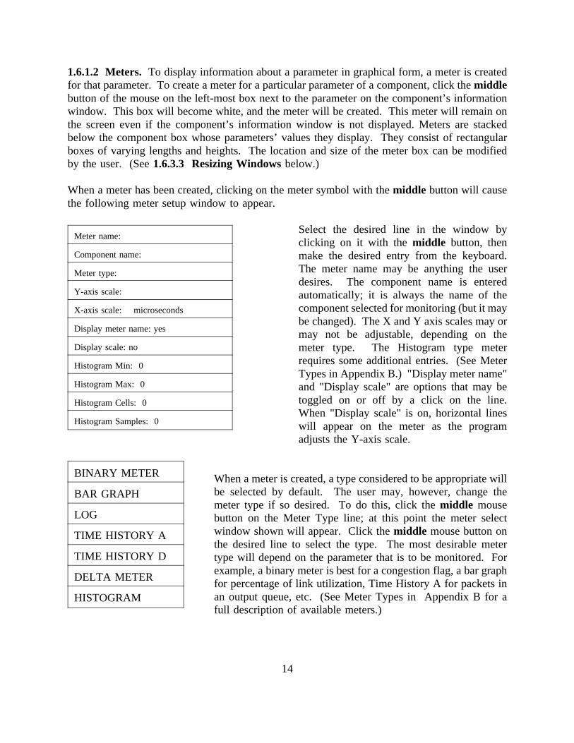
1.6.1.2 Meters. To display information about a parameter in graphical form, a meter is createdfor that parameter. To create a meter for a particular parameter of a component, click themiddlebutton of the mouse on the left-most box next to the parameter on the component’s informationwindow. This box will become white, and the meter will be created. This meter will remain onthe screen even if the component’s information window is not displayed. Meters are stackedbelow the component box whose parameters’ values they display. They consist of rectangularboxes of varying lengths and heights. The location and size of the meter box can be modifiedby the user. (See1.6.3.3 Resizing Windowsbelow.)

When a meter has been created, clicking on the meter symbol with themiddle button will causethe following meter setup window to appear.

Meter name:

Component name:

Meter type:

Y-axis scale:

X-axis scale: microseconds

Display meter name: yes

Display scale: no

Histogram Min: 0

Histogram Max: 0

Histogram Cells: 0

Histogram Samples: 0

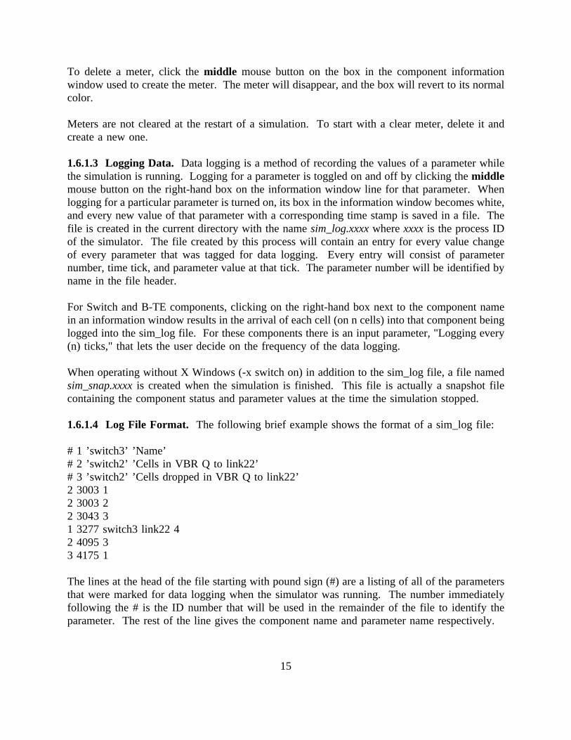
Select the desired line in the window byclicking on it with the middle button, thenmake the desired entry from the keyboard.The meter name may be anything the userdesires. The component name is enteredautomatically; it is always the name of thecomponent selected for monitoring (but it maybe changed). The X and Y axis scales may ormay not be adjustable, depending on themeter type. The Histogram type meterrequires some additional entries. (See MeterTypes in Appendix B.) "Display meter name"and "Display scale" are options that may betoggled on or off by a click on the line.When "Display scale" is on, horizontal lineswill appear on the meter as the programadjusts the Y-axis scale.

BINARY METER

BAR GRAPH

LOG

TIME HISTORY A

TIME HISTORY D

DELTA METER

HISTOGRAM

When a meter is created, a type considered to be appropriate willbe selected by default. The user may, however, change themeter type if so desired. To do this, click themiddle mousebutton on the Meter Type line; at this point the meter selectwindow shown will appear. Click themiddle mouse button onthe desired line to select the type. The most desirable metertype will depend on the parameter that is to be monitored. Forexample, a binary meter is best for a congestion flag, a bar graphfor percentage of link utilization, Time History A for packets inan output queue, etc. (See Meter Types in Appendix B for afull description of available meters.)

14

To delete a meter, click themiddle mouse button on the box in the component informationwindow used to create the meter. The meter will disappear, and the box will revert to its normalcolor.

Meters are not cleared at the restart of a simulation. To start with a clear meter, delete it andcreate a new one.

1.6.1.3 Logging Data. Data logging is a method of recording the values of a parameter whilethe simulation is running. Logging for a parameter is toggled on and off by clicking themiddlemouse button on the right-hand box on the information window line for that parameter. Whenlogging for a particular parameter is turned on, its box in the information window becomes white,and every new value of that parameter with a corresponding time stamp is saved in a file. Thefile is created in the current directory with the namesim_log.xxxxwherexxxx is the process IDof the simulator. The file created by this process will contain an entry for every value changeof every parameter that was tagged for data logging. Every entry will consist of parameternumber, time tick, and parameter value at that tick. The parameter number will be identified byname in the file header.

For Switch and B-TE components, clicking on the right-hand box next to the component namein an information window results in the arrival of each cell (on n cells) into that component beinglogged into the sim_log file. For these components there is an input parameter, "Logging every(n) ticks," that lets the user decide on the frequency of the data logging.

When operating without X Windows (-x switch on) in addition to the sim_log file, a file namedsim_snap.xxxxis created when the simulation is finished. This file is actually a snapshot filecontaining the component status and parameter values at the time the simulation stopped.

1.6.1.4 Log File Format. The following brief example shows the format of a sim_log file:

# 1 ’switch3’ ’Name’# 2 ’switch2’ ’Cells in VBR Q to link22’# 3 ’switch2’ ’Cells dropped in VBR Q to link22’2 3003 12 3003 22 3043 31 3277 switch3 link22 42 4095 33 4175 1

The lines at the head of the file starting with pound sign (#) are a listing of all of the parametersthat were marked for data logging when the simulator was running. The number immediatelyfollowing the # is the ID number that will be used in the remainder of the file to identify theparameter. The rest of the line gives the component name and parameter name respectively.

15

All lines following the ones marked with # are the actual data recorded during the simulation.The first column is the parameter ID, the second column is the time (in ticks), and the thirdcolumn is the value of the parameter at that time. A slightly different format is used for the casewhere the data logged represents cell arrival at a switch or B-TE component. (This is the loggingenabled with the box on the component’s name line.) In this case the third column is the nameof the component on which the data is collected (switch3 in the example). The fourth columnis the name of the link from where the cell arrived (link 22), and the fifth column is the routenumber.

1.6.2 Making Modifications

1.6.2.1 Modifying Components. After it is created, a component can be modified by editingits input parameters. To edit a parameter, pop up the component’s information window byclicking on the symbol with the middle mouse button, then click on the parameter to be edited.A prompt will appear in the text window, at which time the new value of the parameter can beentered.

1.6.2.2 Deleting Components.Deleting components is done with the KILL control button.After clicking on KILL, any component that the user clicks on is deleted. When finisheddeleting components, the user clicks on QUIT to get out of this mode. CAUTION: Failing toclick on QUIT after deleting can be harmful to your configuration; inadvertent deletion ofcomponents may result if the middle button is used for selection without QUITing the deletemode. Also note that clicking on QUIT while in KILL mode does notcause an exit from thesimulator program, but a second click on QUIT willend the session.

It is not possible to delete components once they have been placed in a route (an ATM Virtualchannel). Furthermore, it is not possible to delete a route, thus the user should make every effortto insure that the configuration is constructed as desired before creating the routes.

1.6.3 Manipulating the Network Display

1.6.3.1 Raising/Lowering Windows. Clicking theright mouse button on a window will raise(bring forward) that window so that nothing else on the display will obscure that window.Clicking the left mouse button on a window will lower (push back) that window so that it doesnot obscure any other windows.

1.6.3.2 Moving Windows. Any of the windows in the network display may be repositioned,including components, meters, and information windows. Even the control buttons and clockmay be moved, but only as a group. To accomplish a move, click and hold theright mousebutton on the window, drag the box outline which appears to the new location for the window,and release the mouse button.

16

1.6.3.3 Resizing Windows.It is possible to resize meter windows. To do this, click and holdthemiddle mouse button on one corner of the window. A box outline will appear which can beresized by moving the mouse with the button still depressed. When the box outline is the desiredshape and size, release the mouse button and the window will be resized.

It is also possible to resize the entire simulator window. Its initial size is the full size of thescreen. To change the size or location of the window, use the standard X Window manager(uwm). You must have the lineresizerelativein your .uwmrc file for this to work, however.

1.6.3.4 Resizing Information Windows. Clicking and holding themiddle mouse buttonanywhere inside the information window will cause its dimensions and text to get larger. Toreturn to the normal size, the information window must be closed and reopened.

1.6.4 Saving a Network Configuration

There are two ways to save a network configuration.

The SAVE command allows the user to save the present network configuration. Clickingon the SAVE control button causes the program to prompt the user for a filename underwhich to save the configuration.

The SNAP command does the same thing as SAVE except that it also saves the presentarrangement of meters and information windows on the display. The SNAP commandsaves the temporary values of the components’ parameters.

A detailed description of the formats of both these file types is given inAppendix C.

1.6.5 Post Simulation Analysis using the Log File

In many cases the user will find it desirable to have data on one or more network componentsplotted or otherwise presented for further analysis. One way of doing this is to parse the sim_logfile in order to get a data file with two columns (X, Y) that can be fed into any datasheetprogram such as Lotus 1-2-3, GnuPlot, etc.2 A "filter" program is provided with the simulatorpackage for this purpose. The usage for the filter is as follows:

filter sim_log.xxxx component_name parameter_name

2 Trade names mentioned in the text are meant only to identify typical products. Suchidentification does not imply recommendation or endorsement by the National Institute ofStandards and Technology, nor does it imply the products are necessarily the best availble forthe purpose.

17

The above line will send the filter output to the standard output device; to redirect the output toa file type;

filter sim_log.xxxx component_name parameter_name> output_file

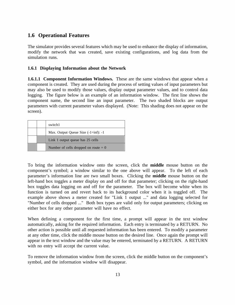
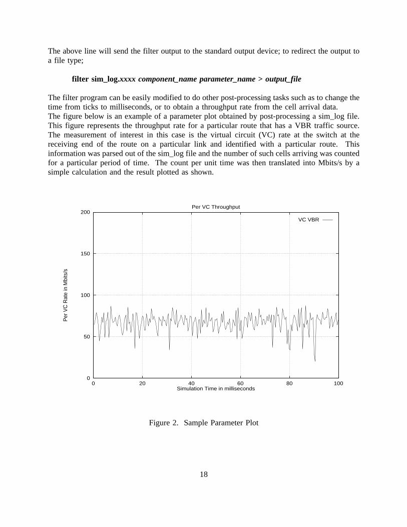
The filter program can be easily modified to do other post-processing tasks such as to change thetime from ticks to milliseconds, or to obtain a throughput rate from the cell arrival data.The figure below is an example of a parameter plot obtained by post-processing a sim_log file.This figure represents the throughput rate for a particular route that has a VBR traffic source.The measurement of interest in this case is the virtual circuit (VC) rate at the switch at thereceiving end of the route on a particular link and identified with a particular route. Thisinformation was parsed out of the sim_log file and the number of such cells arriving was countedfor a particular period of time. The count per unit time was then translated into Mbits/s by asimple calculation and the result plotted as shown.

0

50

100

150

200

0 20 40 60 80 100

Per

VC

Rat

e in

Mbi

ts/s

Simulation Time in milliseconds

Per VC Throughput

VC VBR

Figure 2. Sample Parameter Plot

18

1.7 Simulator Concepts

1.7.1 Simulation Clock

The simulator iseventdriven. Components send each other events in order to communicate andsend cells through the network. The software contains an event manager which provides ageneral facility to schedule and send or "fire" an event. An event queue is maintained in whichevents are kept sorted by time. To fire an event, the first event in the queue is removed, theglobal time is set to the time of that event and any action scheduled to take place is undertaken.Events can be scheduled at the current time or at any time in the future. Scheduling events forthe past is considered illogical. Events scheduled at the same time are not guaranteed to fire inany particular order.

Simulator time is maintained by the event manager in units ofticks. The time is maintained asan unsigned 32-bit value. The simulator time represented by one tick can be changed bysoftware modification (see section 2.3.4), but not by the simulator user. For the present, a tickrepresents 10 nanoseconds. With that value, a total of 42 seconds of simulated time is availablefor one run of the program.

1.7.2 ATM Switch

The switch is the component that switches or routes cells over several virtual channel links. Alocal routing table is provided for each switch. This table contains a route number (that is readfrom incoming cell structure and is the equivalent of the cell’s virtual channel identifier), a nextlink entry, and a next switch/next B-TE entry. Let’s consider a cell arriving at the switch froma physical link. At the next switching slot time, after some delay (set by user), the switch looksin its local routing table to determine which outgoing link it should redirect the cell to. At thispoint, if the link has an empty slot available, the switch puts the cell on the link. If a link slotis not available, the cell awaits transmission in one of the priority queues, namely, the CBR/VBRqueue or the ABR queue, depending on the type of service provided by this virtual channel.Cells in the CBR/VBR queue have priority over cells in the ABR queue, i.e., it is only when theCBR/VBR queue is empty that the ABR traffic is sent. If either queue exceeds a High Thresholdvalue set by the user, a congestion flag for that port is set to True. Both queues must be belowa Low Threshold value for the congestion flag to be reset to False. The Output Queue Size (setby the user) determines the available buffer space for each type of queue (CBR/VBR or ABR).If any queue exceeds the set limit, cells are dropped and this is recorded as a percentage of thetotal number of cells received by the switch. Also, there is a per port cell drop parameterrecorded for each queue.

1.7.3 Broadband Terminal Equipment (B-TE)

The B-TE component simulates a Broadband ISDN node, e.g., a host computer, workstation, etc.A B-TE has one or more ATM Applications at the user side and a physical link on the network

19

side. Cells received from the Application side are forwarded to the physical link. If no slot isavailable for immediate transmission a cell queued in one of two queues, a VBR/CBR queue oran ABR queue. The user can specify the maximum output queue size; if either queue exceedsthis limit cells will be dropped. The parameters that can be monitored for a B-TE are the numberof cells in an output queue and the number of cells dropped at each queue. Also, the totalnumber of cells received from the network may be monitored.

1.7.4 ATM Applications

The ATM application at the end-point of a link is a traffic generator. The traffic source emulatedby this component may be a constant bit rate (CBR) source or a variable bit rate (VBR) source.Either source type may generated at one of two priority levels: a CBR/VBR level (highestpriority) or the Available Bit Rate (ABR) level where cells are sent on the transmissionbandwidth that is available after the higher level traffic has been sent. At each priority levelthere are three types of traffic generators:

1. A constant rate traffic where the user specifies the bit rate. Cells will be generated at thespecified rate for the duration of the simulation.

2. Variable Bit Rate - Poisson. This type of traffic has an ON-OFF source. Both the burstperiod (ON) and the silence period (OFF) are drawn from an exponential distribution.The user specifies the mean burst length, the mean interval between bursts, and the bitrate at which cells are generated during the ON period.

3. Variable Bit Rate - Batch. For this traffic source the user specifies the mean number ofcells generated during a burst and the mean interval between bursts.

For all of the traffic types, the user specifies the start time and the number of megabits to besent.

Another ATM Application type that can be simulated is a TCP/IP application. See Appendix Afor a list of input and output parameters.

1.7.5 Link Components

This component simulates the physical medium (copper wire or optical fiber) on which cells aretransmitted. The user may choose the link speed from a list of several different standard rates.The user also specifies the length of the link. The output parameter reported by the simulatoris link utilization in terms of bit rate (Mbits/s). The measurement of link rate is averaged overa period of 10 cells.

20

PART 2. Programmer’s Guide

2.1 Objectives and Overview

This part of the document briefly describes the ATM Network Simulator Software and theprocedures necessary to make user modifications, such as the creation of new components or tochange the behavior of existing components. It is assumed that the reader is familiar with CLanguage programming techniques, conventions, and notations, and has the source code of theATM Network Simulator available for reference.

The simulator can simulate anything that can be modeled by a network of components that sendmessages to one another. The components schedule events for one another to cause things tohappen. The model being simulated and the action of the components is entirely determined bythe code controlling the components, not by the framework of the simulator. The person whoimplements the components can decide how they will go about having components send messagesto one another; the simulator framework only provides the means to schedule events and tocommunicate with the user.

The simulator program includes a graphical user interface which provides the user with a meansto display the topology of the network, define the parameters and connectivity of the network,log data, and to save and load the network configuration. In addition to the user interface, thesimulator has an event manager, I/O routines, and various tools that can be used to buildcomponents.

21

2.2 Components

The component is the basic building block of the simulator. There are different classes ofcomponents; examples are switches, physical links, terminal equipment, and ATM applications.Some classes allow different types within the class in order to accommodate the simulation ofa variety of implementations. For example, an ATM application may generate traffic at aconstant bit rate, or a variable bit rate that is governed by some particular distribution function.

Every component consists of an action routine and a data structure. All components of the sametype share the same action routine; this routine is called for each event that happens to acomponent. Each instance of a component has its own data structure which is used to storeinformation that characterizes the component plus some standard information required by thesimulator for every component.

2.2.1 Classes and Types

Every component has aclassand atype. A particular class of component may contain severaldifferent types of components. The following are the different classes of components currentlydefined and, in parentheses, the way the names appear in the source filecomptypes.h:

· Links (LINK_CLASS)

· ATM Switches (SWITCH_CLASS)

· Broadband Terminal Equipment (BTE_CLASS)

· ATM Applications (CONNECTION_CLASS)

For now, the Link, Switch, and B-TE classes contain only one type each. Respectively, they are(as defined incomptypes.candcomptypes.h):

· Physical Link (ATMLINK)

· ATM Switch (SWITCH)

· B-TE (BTE)

The ATM Applications class, however, contains many types; these are defined as follows:

· Constant Bit Rate (CBRCONNECTION)

· Variable Bit Rate - Poisson (VBRCONNECTION)

22

· Variable Bit Rate - Batch (BATCHCONNECTION)

· Available Bit Rate - Constant (ABRCONNECTION1)

· Available Bit Rate - Poisson (ABRCONNECTION2)

· Available Bit Rate - Batch (ABRCONNECTION3)

· TCP/IP Application (TCPCONNECTION)

When creating a new type of component,comptypes.candcomptypes.hmust be modified tocontain a new constant for the new component type, and a new entry must be made in thecomp_types[]array.

2.2.2 Component Data Structures

Each instance of a component has a data structure that is used to store any information neededby the component, as well as standard information needed by the simulator for every component.Component structures are kept in a list; the order of the list depends on the order of creation ofthe component. Each differenttypeof component has its own structure which is defined in theheader (.h) file for that type, but the beginning of every component structure is the same. Thisgeneric structure is as follows (actual listing can be found incomponent.h):

typedef struct _Component {struct _Component *co_next, *co_prev; /* Links to other components in list */short co_class; /* Class of component */short co_type; /* Type of component */char co_name[40] /* Name to appear on screen */PFP co_action /* Main function, called with each event */COMP_OBJECT co_picture; /* Graphics object to be displayed on screen */list *co_neighbors; /* Points to a list of neighbors of this component */

/* Parameters -- data that will be displayed on the screen */

short co_menu_up; /* If true, then text window is up */queue *co_params; /* Variable-length queue of parameters */

/* Any other info that a component needs to keep will vary */

} Component;

2.2.3 Parameters

Any information about a component that needs to be displayed on the screen, logged to disk, orsaved in a configuration file must be stored in aparameter. A parameter is a data structure that(besides storing a value) stores information needed to display, save, or load the parameter. The

23

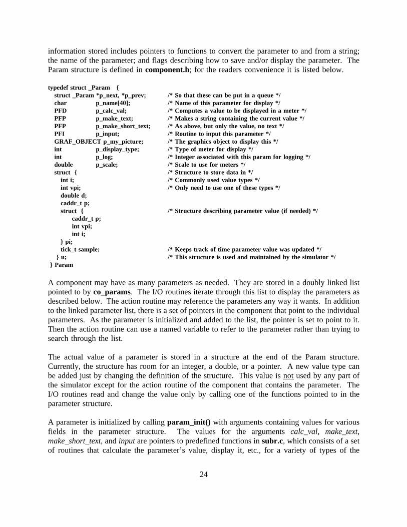
information stored includes pointers to functions to convert the parameter to and from a string;the name of the parameter; and flags describing how to save and/or display the parameter. TheParam structure is defined incomponent.h; for the readers convenience it is listed below.

typedef struct _Param {struct _Param *p_next, *p_prev; /* So that these can be put in a queue */char p_name[40]; /* Name of this parameter for display */PFD p_calc_val; /* Computes a value to be displayed in a meter */PFP p_make_text; /* Makes a string containing the current value */PFP p_make_short_text; /* As above, but only the value, no text */PFI p_input; /* Routine to input this parameter */GRAF_OBJECT p_my_picture; /* The graphics object to display this */int p_display_type; /* Type of meter for display */int p_log; /* Integer associated with this param for logging */double p_scale; /* Scale to use for meters */struct { /* Structure to store data in */

int i; /* Commonly used value types */int vpi; /* Only need to use one of these types */double d;caddr_t p;struct { /* Structure describing parameter value (if needed) */

caddr_t p;int vpi;int i;

} pi;tick_t sample; /* Keeps track of time parameter value was updated */

} u; /* This structure is used and maintained by the simulator */} Param

A component may have as many parameters as needed. They are stored in a doubly linked listpointed to byco_params. The I/O routines iterate through this list to display the parameters asdescribed below. The action routine may reference the parameters any way it wants. In additionto the linked parameter list, there is a set of pointers in the component that point to the individualparameters. As the parameter is initialized and added to the list, the pointer is set to point to it.Then the action routine can use a named variable to refer to the parameter rather than trying tosearch through the list.

The actual value of a parameter is stored in a structure at the end of the Param structure.Currently, the structure has room for an integer, a double, or a pointer. A new value type canbe added just by changing the definition of the structure. This value is notused by any part ofthe simulator except for the action routine of the component that contains the parameter. TheI/O routines read and change the value only by calling one of the functions pointed to in theparameter structure.

A parameter is initialized by callingparam_init() with arguments containing values for variousfields in the parameter structure. The values for the argumentscalc_val, make_text,make_short_text, andinput are pointers to predefined functions insubr.c, which consists of a setof routines that calculate the parameter’s value, display it, etc., for a variety of types of the

24

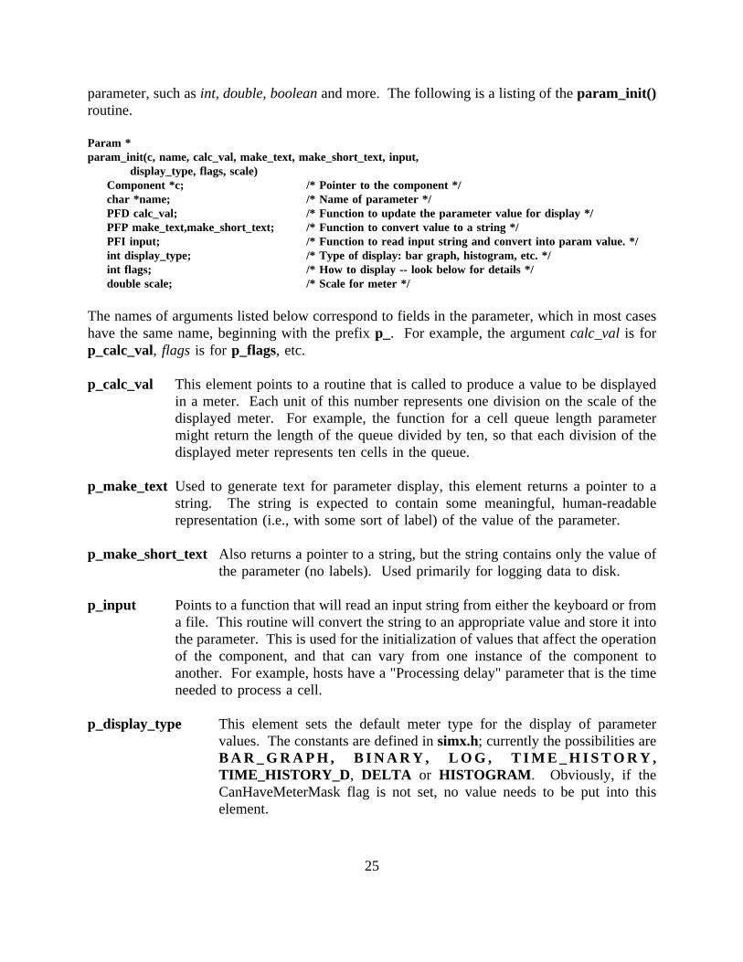
parameter, such asint, double, booleanand more. The following is a listing of theparam_init()routine.

Param *param_init(c, name, calc_val, make_text, make_short_text, input,

display_type, flags, scale)Component *c; /* Pointer to the component */char *name; /* Name of parameter */PFD calc_val; /* Function to update the parameter value for display */PFP make_text,make_short_text; /* Function to convert value to a string */PFI input; /* Function to read input string and convert into param value. */int display_type; /* Type of display: bar graph, histogram, etc. */int flags; /* How to display -- look below for details */double scale; /* Scale for meter */

The names of arguments listed below correspond to fields in the parameter, which in most caseshave the same name, beginning with the prefixp_. For example, the argumentcalc_val is forp_calc_val, flags is for p_flags, etc.

p_calc_val This element points to a routine that is called to produce a value to be displayedin a meter. Each unit of this number represents one division on the scale of thedisplayed meter. For example, the function for a cell queue length parametermight return the length of the queue divided by ten, so that each division of thedisplayed meter represents ten cells in the queue.

p_make_text Used to generate text for parameter display, this element returns a pointer to astring. The string is expected to contain some meaningful, human-readablerepresentation (i.e., with some sort of label) of the value of the parameter.

p_make_short_text Also returns a pointer to a string, but the string contains only the value ofthe parameter (no labels). Used primarily for logging data to disk.

p_input Points to a function that will read an input string from either the keyboard or froma file. This routine will convert the string to an appropriate value and store it intothe parameter. This is used for the initialization of values that affect the operationof the component, and that can vary from one instance of the component toanother. For example, hosts have a "Processing delay" parameter that is the timeneeded to process a cell.

p_display_type This element sets the default meter type for the display of parametervalues. The constants are defined insimx.h; currently the possibilities areB A R _ G R A P H , B I N A R Y , L O G , T I M E _ H I S T O R Y ,TIME_HISTORY_D , DELTA or HISTOGRAM . Obviously, if theCanHaveMeterMask flag is not set, no value needs to be put into thiselement.

25

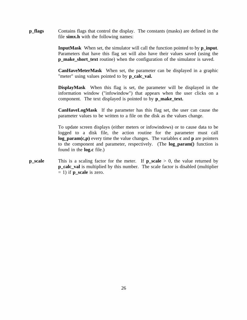
p_flags Contains flags that control the display. The constants (masks) are defined in thefile simx.h with the following names:

InputMask When set, the simulator will call the function pointed to byp_input.Parameters that have this flag set will also have their values saved (using thep_make_short_textroutine) when the configuration of the simulator is saved.

CanHaveMeterMask When set, the parameter can be displayed in a graphic"meter" using values pointed to byp_calc_val.

DisplayMask When this flag is set, the parameter will be displayed in theinformation window ("infowindow") that appears when the user clicks on acomponent. The text displayed is pointed to byp_make_text.

CanHaveLogMask If the parameter has this flag set, the user can cause theparameter values to be written to a file on the disk as the values change.

To update screen displays (either meters or infowindows) or to cause data to belogged to a disk file, the action routine for the parameter must calllog_param(c,p)every time the value changes. The variablesc andp are pointersto the component and parameter, respectively. (Thelog_param() function isfound in thelog.c file.)

p_scale This is a scaling factor for the meter. Ifp_scale> 0, the value returned byp_calc_val is multiplied by this number. The scale factor is disabled (multiplier= 1) if p_scaleis zero.

26

2.2.4 Neighbors

Neighbors are stored as a list ofNeighbor structures; this list is pointed to from componentstructures. Each neighbor structure contains a pointer to the neighboring component, a queue inwhich to store cells (if needed), a busy flag, and a pointer to a parameter to display anything thatmight be associated with the neighbor. The definition of the Neighbor structure is listed below;it can be also be found incomponent.h.

typedef struct_Neighbor {struct_Neighbor

*n_next, *n_prev; /* Links for the list */Component *n_c; /* Pointer to the neighboring component */

/* The next values will vary from network to network, and from component to component. For example, onlyswitches and hosts have queues in the current application. */

queue *n_pq; /* Queue of packets to be sent */short n_busy; /* True if neighbor is busy */double n_prev_sample; /* Previous sample time used for utilization calculation in links */Param *n_p; /* Index of parameter to display whatever */Param *n_pp; /* Index of parameter to display whatever */Param *n_ppp;list *n_vpi /* List of parameters related to vpi number of the different routes */caddr_t n_data; /* If a component wants to store arbitrary data for each neighbor, put

it here. */} Neighbor;

When a neighbor is added, the component must create and initialize a neighbor structure, and putit on its neighbors list. If there is some piece of information associated with the neighbor thatmust be displayed, a parameter structure must be allocated, initialized appropriately, and addedto the queue of parameters in the component structure. See the functionb_neighbor() in bte.cfor an example of usage. The following is defined insubr.c and can be used when writing anew routine to give it the capability to add neighbors.

Neighbor *add_neighbor(c, neighc, max_num_neighbors, num_classes)

Component *c; /* Comp to add neighbor to */Component *neighc; /* New neighbor */int max_num_neighbors; /* Max number neighbors allowed (0=infinite) */int num_classes; /* How many classes follow */

Similarly, the following is also defined insubr.c and can be used to provide a routine with thecapability to remove neighbors.

remove_neighbor(c, neighc)Component *c, *neighc;

27

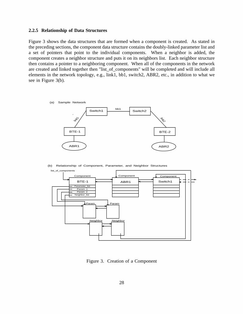
2.2.5 Relationship of Data Structures

Figure 3 shows the data structures that are formed when a component is created. As stated inthe preceding sections, the component data structure contains the doubly-linked parameter list anda set of pointers that point to the individual components. When a neighbor is added, thecomponent creates a neighbor structure and puts it on its neighbors list. Each neighbor structurethen contains a pointer to a neighboring component. When all of the components in the networkare created and linked together then "list_of_components" will be completed and will include allelements in the network topology, e.g., link1, bb1, switch2, ABR2, etc., in addition to what wesee in Figure 3(b).

NeighborNeighbor

Param Param

Neighbor_list

Param 1Param 2

Parameter_list

Component Component Component

list_of_components

BTE-1 ABR1 Switch1

(b) Relationship of Component, Parameter, and Neighbor Structures

(a) Sample Network

BTE-1

Switch1 Switch2

BTE-2

ABR2

bb1

link1 link2

ABR1

Figure 3. Creation of a Component

28

2.2.6 Action Routines

As previously stated, every component contains anaction routine. This routine is called for eachevent that happens to a component. (Events are explained in a later section of this document.)The action routine is called (usually not by the event manager, but rather by the action routinethat scheduled the event), to execute a set of commands that will give the component its uniquebehavior. The writer of a component can create components with any sort of behavior.Components can send any type of events to one another. However, in order to allow thesimulator to do various housekeeping functions, every action routine must respond to a minimum,fixed set of commands. A synopsis of the action routine and the commands it is expected toperform is as follows:

/* All of these include files may not be needed, but they are thecommon ones. */

#include <sys/types.h>#include <stdio.h>#include "sim.h"#include "log.h"#include "q.h"#include "list.h"#include "simx.h" /* X window stuff & also component.h */#include "comptypes.h" /* The types of components */#include "cell.h"#include "eventdefs.h" /* Types of events & commands defined here */#include "event.h"#include "this_component_type.h"

/* ------ Definition of some Local Events, if needed -------- */caddr_taction(src, comp, type, cell, vpi, arg)Component *src; /* Component that sent this event. Null for cmds. */Component *comp; /* Component to which this event/cmd applies. */int type; /* Type of event or cmd that is happening. */Cell *cell; /* A cell. */VPI *vpi; /* VPI number of data cell wherever it is applicable. */caddr_t arg; /* Whatever */{

/* Usually a large switch statement on the event type */}

An example of the "large switch statement" referred to in the last comment line above is shownin the code below which is extracted from the action routine for BTE (bte.c). The switchstatement contains a "case" for every type of event to which the component is expected torespond. These include the events for component creation, routing, and initialization, as well asthe basic function of giving the component the ability to pass cells. The example demonstratesthe usual way to transmit a cell, that is, to pass it with anEV_RECEIVE event to anothercomponent. The transmitting component callsev_enqueue (EV_RECEIVE, src, dest, time, rtn,ce, arg)which has as one of its parameters a pointer to the cell,ce. When the resulting event,after being queued in the event list, gets "fired," the action routine of the destination component

29

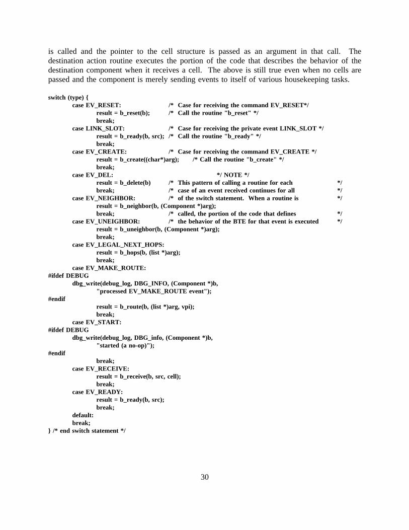
is called and the pointer to the cell structure is passed as an argument in that call. Thedestination action routine executes the portion of the code that describes the behavior of thedestination component when it receives a cell. The above is still true even when no cells arepassed and the component is merely sending events to itself of various housekeeping tasks.

switch (type) {case EV_RESET: /* Case for receiving the command EV_RESET*/

result = b_reset(b); /* Call the routine "b_reset" */break;

case LINK_SLOT: /* Case for receiving the private event LINK_SLOT */result = b_ready(b, src); /* Call the routine "b_ready" */break;

case EV_CREATE: /* Case for receiving the command EV_CREATE */result = b_create((char*)arg); /* Call the routine "b_create" */break;

case EV_DEL: */ NOTE */result = b_delete(b) /* This pattern of calling a routine for each */break; /* case of an event received continues for all */

case EV_NEIGHBOR: /* of the switch statement. When a routine is */result = b_neighbor(b, (Component *)arg);break; /* called, the portion of the code that defines */

case EV_UNEIGHBOR: /* the behavior of the BTE for that event is executed */result = b_uneighbor(b, (Component *)arg);break;

case EV_LEGAL_NEXT_HOPS:result = b_hops(b, (list *)arg);break;

case EV_MAKE_ROUTE:#ifdef DEBUG

dbg_write(debug_log, DBG_INFO, (Component *)b,"processed EV_MAKE_ROUTE event");

#endifresult = b_route(b, (list *)arg, vpi);break;

case EV_START:#ifdef DEBUG

dbg_write(debug_log, DBG_info, (Component *)b,"started (a no-op)");

#endifbreak;

case EV_RECEIVE:result = b_receive(b, src, cell);break;

case EV_READY:result = b_ready(b, src);break;

default:break;

} /* end switch statement */

30

2.3 Events

The simulator is event driven — the event queue is a queue of events kept sorted by time. Tofire an event, the first event in the queue is removed, the global time is set to the time of thatevent, and the action routine pointed to in the event structure is called. When the user clicks onthe START button, each component is sent a reset command followed by a start command, thenthe simulator enters a loop. The loop processes any X events, updates the display, then fires allthe events at the head of the event queue that have the same time.

Currently, there are three classes of events: commands, regular events, and private events.Commands and regular events are defined ineventdefs.h. Commands are those events whichperform some action such as reset, start, create, etc., while regular events are those which areconcerned with the actual running of the simulation, e.g., receive, ready, busy. Private eventsare events that components send to themselves, therefore they are defined in the source files ofthe components, rather than in a central location.

2.3.1 Command Set (EV_CLASS_CMD)

All components must accept the following commands. The component need not actually use thecommand but should respond in an orderly and predictable way when the command is received.When used in an action routine, the action routine should return NULL if an error occurs duringa command, and something that is non-NULL otherwise.

EV_CREATE Create a new instance of a component. Thecomp variable must be NULL,argpoints to the name of the new component, and the action routine returns either a pointer to a newdata structure or NULL for error. The action routine must allocate the correct amount of memoryfor the new component’s data structure, create its (empty) neighbor list, create the queue ofparameters, create any cell queues, etc. This command must also initialize all the private datain the component as necessary. The only information that need not be initialized are anyparameters with theInputMask flag set. They will be initialized by the simulator as specifiedin the Parameters section of this document.

EV_DEL Delete an instance of component. This command will detach the component from anyneighbors it has, free any storage associated with the component, including its data structure, andperform any other necessary clean-up.

EV_RESET Reset the state of the component — clear out any cell queues, forget about anycells being processed, etc. When the START button of the simulator is hit,EV_RESET is calledfirst for all components and thenEV_START.

EV_START Start operations — for example, start a cell generator sending cells. For manycomponents, this will be a no-op.

31

EV_NEIGHBOR Attach another component as a new neighbor. The component to be madea neighbor is pointed to byarg. A component should only allow legal neighbors. For example,an ATM Application will not allow an ATM Switch to be attached as a neighbor — the ATMApplication can only be connected to a B-TE (Broadband-ISDN Terminal).

EV_UNEIGHBOR Remove the neighbor pointed to byarg from the list of neighbors, and freeany memory used to keep track of the neighbor (such as a cell queue and the neighbor structureitself). If there is a parameter associated with this neighbor, it must be removed from the queueof parameters and freed. This is a no-op if the component is not a neighbor.

EV_LEGAL_NEXT_HOPS arg points to anl list (see the section 2.5.1, Lists and Queues, foran explanation of anl list) that contains a virtual channel connection being constructed (notincluding comp). The list contains only the components in the path so far.comp is thecomponent being considered as the next step in the connection. The action routine must returna new list of the components that are legal in the path aftercomp. A NULL list indicates anerror, an empty list means thatcomp is not legal for the virtual channel connection so far, thatthere is no legal next virtual channel link, or thatcomp is the end of the channel. The caller willlq_delete the returned list after it is done with it.

This command is used by the X I/O routines to allow the user to build only legal connections.The X routines know that a component of type ATM Application must be at the beginning ofa virtual channel. When the user picks an ATM Application, the X routine calls that componentaction routine with this command to find out which components are allowed to be next on thepath. As the user picks more components, the process continues until he/she picks another ATMApplication to end the path.

EV_MAKE_ROUTE This command is a no-op for some components like physical links. ATMApplications and B-TEs use it to store the route number in the VCI field of their componentstructures. The ATM Switch component creates a local routing table and stores the previous andnext component and the VCI number of the route.

2.3.2 Regular Events (EV_CLASS_EVENT)

The following events are those which are directly involved in the running of the simulation. Itis necessary to have a set of regular events that are understood by allcomponents in order tofacilitate global communication within the simulator. Additional regular events may be definedif needed. To define a new event, just put a new#define statement into theeventdefs.hfile.

EV_RECEIVE Receive a cell event.

EV_READY Component ready signal.

EV_BUSY Component busy signal.

32

2.3.3 Private Events

Private events are events that have only local significance, i.e., they are defined within actionroutine for use by that routine only. Private events are the means by which an action routine cansend events to itself.

2.3.4 The Event Manager

Components send each other events in order to communicate and send cells through the network.The event manager provides a general facility to schedule and send events. The primaryfunctions of this facility are the maintenance of simulator time and the control of event queueing.

Simulator time is maintained by the event manager in units ofticks. Currently, ONE tick is 10nanoseconds. Once a tick is defined in microseconds or in nanoseconds it is easy to convert thisvalue to seconds, milliseconds, etc. To convert from ticks to microseconds, use theTICKS_TO_USECS macro defined insim.h. To convert from microseconds to ticks, useUSECS_TO_TICKS. Analogous macros exist for nanoseconds and full seconds (representedas doubles). The current time (in ticks) is returned by the functionev_now(). The time ismaintained as an unsigned 32-bit value, so at 10 nanoseconds per tick a total of 42 seconds ofsimulated time is available for one run of the program. If longer simulation runs are requiredthe tick definition may be changed. At ten microseconds per tick, for example, the simulator canrun for almost 12 hours of simulated time. Insim.h there is atypedef called tick_t which hasthe tick definition in microseconds. For the current definition of 10 nanoseconds, the definitionline is #define USECS_PER_TICK 0.01.

The only other event-related function that a component needs to know about isev_enqueue().This function creates a new event and places it in the event queue to be fired at the proper time.ev_enqueue()returns a pointer to the newly created event. The arguments correspond to theones passed to the action routine that will receive the event. The syntax ofev_enqueue()is asfollows:

Event *ev_enqueue(type, src, dest, time, rtn, ce, vpi, arg)

int type; /* Type of event -- e.g EV_RECEIVE,EV_CREATE etc */Component *src; /* Component which issues this command */Component *dest; /* Component on which command applies */tick_t time; /* Time at which the event should be scheduled */PFP rtn; /* The action routine of the destination component */Cell *ce; /* Pointer to a cell*/VPI vpi; /* Route number if a cell is passed */caddr_t arg; /* Can be anything */

Note: PFP is a Pointer to a Function that returns a Pointer, and is defined incomponent.h; rtnis therefore the action routine to call when the event is fired. The argumentsce and arg areoptional — they may be replaced by NULL if no cell is being sent and no information needs tobe passed.

33

You may schedule events at the current time or at any future time. (Scheduling events for thepast is considered illogical.) There is no control over the order, e.g. FIFO or LIFO, of executionof events that are scheduled to fire at the same time. Hence, events scheduled at the same timeare not guaranteed to fire in any particular order.

There also exists a function tounscheduleevents, i.e., remove events from the queue. Selectionof events to be removed may be done according to source and destination components and type,or according to a particular event expiration time.

voidev_dequeue_by_comp_and_type(src, dest, type)

Component *src, *dest;Evtype type;

{/* Remove from the queue any subset of events with particular

source and destination components and type.A NULL source or destination matches all components. */

}

voidev_dequeue_by_time(t)

tick_t t;{

/* Remove from the queue all events due to expire at a particular time t. */}

Again, it should be noted that the designer of components for the simulator is free to usewhatever convention he/she desires for communication between components. The simulator justprovides the ability to send events — what the events mean is up to you. See the section onComponentsfor the conventions now used.

34

2.4 ATM Network-Related Issues

2.4.1 ATM Cell Definition

Since the simulator is designed to simulate ATM networks, acell data type has been defined.A cell constitutes a very important data type in the simulator because it contains the routenumber needed for routing by ATM switches. A cell is a data structure, defined in the filecell.h.The structure may contain different elements to tailor the cell for different applications, but mustalways contain the route number. For switching or routing purposes, an ATM switch reads offthe route number found in the cell, then looks up its routing table to forward the cell via the nextlink to the next switch (or to the next B-TE if at the end of a connection).

The cell data structure is not constrained to be any particular format. Of course, if you are onlymodifying some existing components you should not remove any elements from the structure,but if you are writing a set of components from scratch, a cell can contain anything. To changethe contents of a cell, just change the definition incell.h and recompile. The following is asimple example of a cell structure:

typedef struct_Cell { /* Define cell structure */struct _Cell *cell_next; /* Pointer for use by the queue the cells will be stored in */VPI vpi; /* Route number (virtual path identifier) */PTI pti; /* Payload type identifier */struct cell_payload { /* Structure for the payload portion */Packet *tcp_ip_info; /* The payload will */AAL5_Trailer len; /* be any one of */RM rm; /* these three types */} u; /* Structure */} Cell

An event may include a cell, and most simulation events (as opposed to housekeepingcommands) do so. Normally, cells are transmitted from one component to another by having thetransmitting component call a routine (ev_enqueue) which creates a new event and places it ina queue to be fired at the appropriate time. The receiving component must be able to processthe event in order to receive the cell. This process is explained in more detail in the Eventssection of this document.

A module to handle the allocation and deallocation of cells is provided in the package. Themodule keeps track of all the cells, so that when the simulator is reset all cells can be freed inone step. cell_alloc() returns a new cell,cell_free() frees a cell, andcell_free_all() frees allcells.

The simulator obeys the convention that all components must dispose of all cells that they receivein one way or another. In other words, a component that receives a cell must either callcell_free()on the cell orsend the cell to someone else, but not both. Furthermore, a componentthat sends a cell to someone else should no longer refer to that cell. If it wants to save the cell

35

for some reason (if the cell might be retransmitted, for example), the component must callcell_alloc() and make a copy of the cell.

2.4.2 Setting Up the ATM Virtual Channel

The simulator implements static connections. An ATM channel begins and ends with acomponent of the typeATM APPLICATION . A particular Application can have a route to onlyone other Application. When the user clicks on an ATM Application that is at the other end ofthe virtual channel (this is done while making the route), the routing table at each ATM Switchis updated and information about the next link and the next ATM Switch found on the path isstored.

The file route.c contains a couple of functions to manipulate connections. To determine whereto route a cell next, the function

Route_info *rt_lookup(some arguments)/* ..*/

can be called from an ATM Switch action routine; this should return the next link and nextswitch. The routing process starts whenio() within IO.c callsmake_route_event_handler(bevent)which is found inroute.c. The routing process involvescreating aroute_list, which is a list of components. When finally the user clicks on acomponent of typeATM APPLICATION which is at the end of a route, all switches found inroute_list call their respectiveaction_routines to update their local routing modules.

36

2.5 Tools

2.5.1 Lists and Queues

Lists (doubly-linked lists) and queues (singly-linked lists) are used extensively throughout thesimulator. Lists and queues contain variables to store the current, maximum and minimum lengthof the list/queue. A list has the following structure:

typedef struct list { /* list header */l_elt *l_head; /* first element in list */l_elt *l_tail; /* last element in list */int l_len; /* number of elements in queue */int l_max; /* maximum length */int l_min; /* minimum length */

} list;

An element in the list,l_elt, has the following structure:

typedef struct l_elt { /* list element */struct l_elt *le_next, *le_prev; /* Links */caddr_t le_data;

} l_elt;

Because both lists that were efficient and lists that were flexible were needed, there are two kindsof lists. One kind requires that the item being placed on the list contain the pointers needed tolink it into the list. This means that no extra memory is needed to put the new item into the list.However, this also means that the item being placed on the list must include room for one or twopointers at the beginning, and it can only be on one list at a time. Since the item itself containsthe pointers, the pointers for the first list will be overwritten when it is placed on a second list.This type of list we have chosen to call anle list (or aqe queue). The le stands forlist element,and it means that the items being placed in the list already have the pointers for a list elementbuilt in. As an example, the global list of components is anle list and the component structurecontains two pointers (the structure elementsco_nextandco_prev).

The other kind of list allocates a small area of memory in which to store the pointers every timea new element is added to a list. This means that adding and removing items from the list isslower, but any type of data structure (even ones that don’t have pointers at the beginning) canbe placed on any number of lists any number of times. This type of list is called anl list (or aq queue).

Functions (and macros) that start withle_ andqe_are the faster routines, and the ones that startwith l_ andq_ are the more general ones. (With one exception:l_create() serves both typesof list.) In the arguments to the functions,l andq indicate a list and a queue, respectively, andany other arguments are elements on which to operate. Here is a summary of the available listand queue commands:

37

l_create() Create a new, empty list and return it. Returns NULL on error.

l{e}_addh(l, elt) Add elt to the head of the listl. The le version does not returnanything (it is a macro); thel type returns NULL on error (couldn’tallocate memory to hold the pointers), non-NULL otherwise.

l{e}_addt(l, elt) As above, but addelt to the tail of the list l.

l{e}_remh(l) Remove the item at the head of the list and return it.

l{e}_remt(l) Remove the item at the tail of the list and return it.

l{e}_adda(l, prev, new) Add new to the list afterprev, which must already be in the list.Again, thele is a macro that doesn’t return anything, andl_adda()returns NULL on error.

l{e}_del(l, elt) Deleteelt from the list l.

l_find(l, elt) Search forelt in the list. Returns a pointer to thel_elt thatcontainselt. An l_elt is the structure that contains the pointersused to add something to anl list. Seelist.h for the definition.

lq_delete(l) This function works for both lists and queues. It also works forboth flavors of each, although the effect is slightly different. Forle lists, lq_delete() frees the list andthe elements that were storedin the list. Forl lists, the function does notfree the items storedin the list, just the list and associated extra garbage.

lq_clear(l) As with lq_delete(), this function works for both lists and queues.This function removes all the items from a list or queue. If it is ale list or qe queue, the memory for the items is also freed,otherwise they are merely removed from the list or queue.

l_obliterate() This function is only forl lists. It frees the list, thel_elts used bythe list, andthe data blocks (which must have been allocated usingmalloc() or calloc()).

The following functions perform the same actions on queues as the similarly-named functionsfor lists:

q_create()q{e}_addh(q, elt)

38

q{e}_addt(q, elt)q{e}_adda(q, prev, new)q{e}_del(q, elt)q_find(q, elt)

Finally, queues have the following operations of their own:

q{e}_deq(q) Removes and returns the item at the head of the queue.

qe_find(q, qe) Looks for the itemqe in the queue. Returnsqe if found, NULL otherwise.

qe_dela(q, prev) Removes the element afterprev in q. This operation isO(1), unlikeq{e}_del() which is O(n).

2.5.2 Other Tools

In addition to lists and queues, the simulator includes a hash table module and a module tocontrol allocation of fixed-size memory blocks. The functions for these modules are containedin hash.c, hash.h, mempool.c, andmempool.h.

The hash table is fairly straight-forward. Its functions are described in comments at thebeginning ofhash.c.

The "mempool" was originally written to try to speed up the simulator by avoidingcalloc() andfree() calls. However, no real speed advantage was noted. This module is still useful though,because it makes it possible to free all allocated memory chunks with one call. Cells and eventsare allocated using this module, and of course anyone else may use it as well. The functions ofthe mempool module are relatively easy to understand and are described at the beginning ofmempool.c.

2.5.3 Debugging

There are several ways to do debugging. There are two ways that are convenient to use with thesimulator:

· Include additional code for debugging which is enclosed between#ifdef DEBUG .....#endif DEBUG, define the flagDEBUG for the C-compiler, and set the debug-level bydbg_set_level(DBG_ERR)or dbg_set_level(DBG_INFO)to trace certain actions.

· The arrival of cells at a certain component can be recorded by callinglog_a_cell(c, p, ce)defined inlog.c. In order to properly print the contents of a cell, it might be necessaryto modify this function according to the type of cell that is displayed.

39

40

2.6 Creating New Versions

To create a new version of the simulator by adding your own component to it, all you need islibsim.a, any simulator header files that your new component needs,comptypes.c, and the sourceto your component.

In brief, you must take the following steps to create a new type of component. (It is assumed thatyou have already built the simulator librarylibsim.a and the executable with the distributedcomponents to make sure that it all works.)

1. Modify comptypes.cand comptypes.h to contain a new constant for the new type ofcomponent, a new entry in thecomponent_types[]array, and a declaration of the actionroutine.

2. Create a new component structure, putting it in its own .h file, saynewcomp.h. Theeasiest way to do this is to look at one of the existing component structures and modifyit as necessary. Be sure to readcomponent.h for a description of the commoncomponent structure that all simulator components must share. This shared part of thestructure must exist and be the same for all components. Parameters and the private partof the structure can be modified as desired.

3. Create an action routine for the component. Again, the easiest way to do this is to usethe code from an existing component as a model. Also see the descriptions in thisdocument of the various commands that an action routine must perform. If the newcomponent will interact with the components that are already written, it must deal withthe events that they will send it, and it must send them events that they are expecting.Otherwise, it can act in whatever way it wants.

4. Add an object picture (or choose one from among the object pictures provided). Whena component is created the routinecreate_component(found in edit.c) is called fromIO.c. This routine, given the typeof component to be created, will call the appropriateroutine to draw the component on the screen. To change the shape of the component, oneneeds to write the routine that will draw the component (for example, seepop_comp_windowin components.c).

5. Change theMakefile, to make sure the new components are compiled and linked into thesimulator. For a simple component, it should suffice to addnewcomp.o to theADDLOBJS macro in the makefile. In fact, the following command line should be ableto build a new simulator without modifying the Makefile:

make ADDLOBJS=newcomp.c custom_sim

If you want dependencies on header files and/or any special rules for making your newcomponent, you will have to change the makefile.

41

42

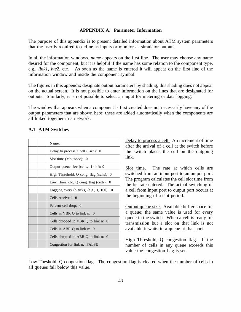
APPENDIX A: Parameter Information

The purpose of this appendix is to present detailed information about ATM system parametersthat the user is required to define as inputs or monitor as simulator outputs.

In all the information windows,nameappears on the first line. The user may choose any namedesired for the component, but it is helpful if the name has some relation to the component type,e.g., link1, bte2, etc. As soon as the name is entered it will appear on the first line of theinformation window and inside the component symbol.

The figures in this appendix designate output parameters by shading; this shading does not appearon the actual screen. It is not possible to enter information on the lines that are designated foroutputs. Similarly, it is not possible to select an input for metering or data logging.

The window that appears when a component is first created does not necessarily have any of theoutput parameters that are shown here; these are added automatically when the components areall linked together in a network.

A.1 ATM Switches

Delay to process a cell.An increment of timeName:

Delay to process a cell (usec): 0

Slot time (Mbits/sec): 0

Output queue size (cells, -1=inf): 0

High Threshold, Q cong. flag (cells): 0

Low Threshold, Q cong. flag (cells): 0

Logging every (n ticks) (e.g., 1, 100): 0

Cells received: 0

Percent cell drop: 0

Cells in VBR Q to link n: 0

Cells dropped in VBR Q to link n: 0

Cells in ABR Q to link n: 0

Cells dropped in ABR Q to link n: 0

Congestion for link n: FALSE

after the arrival of a cell at the switch beforethe switch places the cell on the outgoinglink.

Slot time. The rate at which cells areswitched from an input port to an output port.The program calculates the cell slot time fromthe bit rate entered. The actual switching ofa cell from input port to output port occurs atthe beginning of a slot period.

Output queue size.Available buffer space fora queue; the same value is used for everyqueue in the switch. When a cell is ready fortransmission but a slot on that link is notavailable it waits in a queue at that port.

High Threshold, Q congestion flag.If thenumber of cells in any queue exceeds thisvalue the congestion flag is set.

Low Theshold, Q congestion flag.The congestion flag is cleared when the number of cells inall queues fall below this value.

43

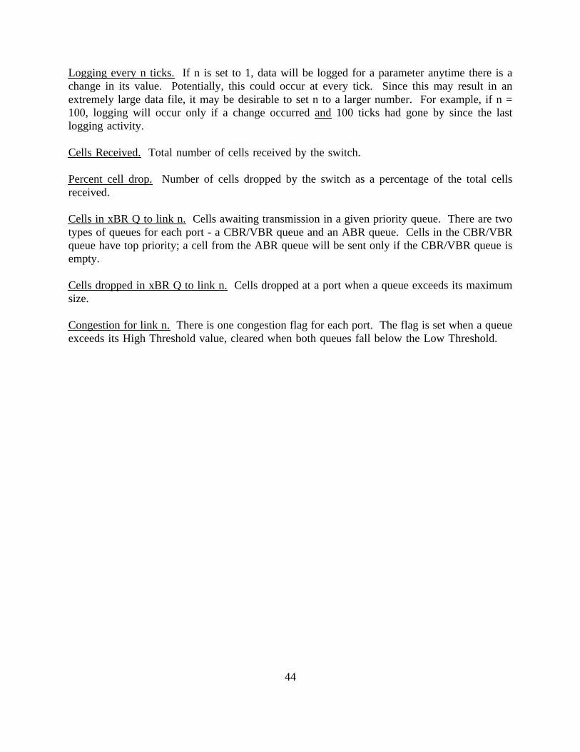
Logging every n ticks. If n is set to 1, data will be logged for a parameter anytime there is achange in its value. Potentially, this could occur at every tick. Since this may result in anextremely large data file, it may be desirable to set n to a larger number. For example, if n =100, logging will occur only if a change occurred and100 ticks had gone by since the lastlogging activity.

Cells Received.Total number of cells received by the switch.

Percent cell drop. Number of cells dropped by the switch as a percentage of the total cellsreceived.

Cells in xBR Q to link n. Cells awaiting transmission in a given priority queue. There are twotypes of queues for each port - a CBR/VBR queue and an ABR queue. Cells in the CBR/VBRqueue have top priority; a cell from the ABR queue will be sent only if the CBR/VBR queue isempty.

Cells dropped in xBR Q to link n.Cells dropped at a port when a queue exceeds its maximumsize.

Congestion for link n.There is one congestion flag for each port. The flag is set when a queueexceeds its High Threshold value, cleared when both queues fall below the Low Threshold.

44

A.2 Broadband Terminal Equipment (B-TE)

Unlike a switch, there can be only one physical link attached to a B-TE component. Cellsreceived from the Application side (there may be multiple Applications) are queued in one of twopriority queues if no link slot is available for transmission. If either queue exceeds its size limitcells will be dropped.

Maximum Output Queue Size. AvailableName:

Max. Output Queue Size (-1=inf): 0

Logging every (n ticks)(e.g., 1, 100): 0

Cells Received: 0

Cells in VBR Q to link n: 0

Cells dropped in VBR Q to link n: 0

Cells in ABR Q to link n: 0

Cells dropped in ABR Q to link n: 0

buffer space for each type of queue.

Logging every n ticks. If n is set to 1, datawill be logged for a parameter anytime thereis a change in its value. Potentially, thiscould occur at every tick. Since this mayresult in an extremely large data file, it maybe desirable to set n to a larger number. Forexample, if n = 100, logging will occur onlyif a change occurred and100 ticks had goneby since the last logging activity.

Cells Received.Total number of cells received by the B-TE.

Cells in xBR Q to link n. Cells awaiting transmission in a given priority queue. There are twotypes of queues - a CBR/VBR queue and an ABR queue. Cells in the CBR/VBR queue havetop priority; a cell from the ABR queue will be sent only if the CBR/VBR queue is empty.

Cells dropped in xBR Q to link n.Cells dropped at the network port when a queue exceeds itsmaximum size.

45

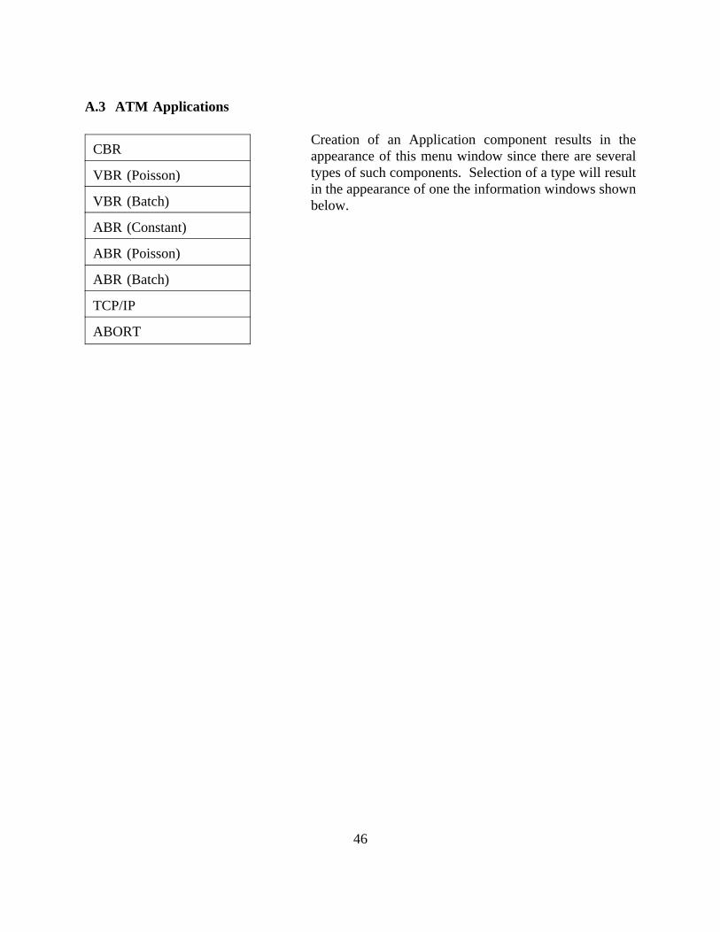
A.3 ATM Applications

Creation of an Application component results in theCBR

VBR (Poisson)

VBR (Batch)

ABR (Constant)

ABR (Poisson)

ABR (Batch)

TCP/IP

ABORT

appearance of this menu window since there are severaltypes of such components. Selection of a type will resultin the appearance of one the information windows shownbelow.

46

For these information windows, the shaded line is not an output parameter; it is the name of theATM Application at the other end of the route. The name is filled in automatically when theroute is created.

All ATM Applications have an input parameter labeledStart Time. This is the number ofmicroseconds after the program starts that the Application will begin generating cells. By settingthe start time to a different value for each Application the user can ensure that they all do notstart at once.

Constant Bit Rate (CBR) Information Window

Name:

Bit Rate (Mbits/sec): 0

Start time (usec): 0

Number of Mbits to be sent: 0

Other End Connection: Name

Cells are generated at a constant rate for theduration of the simulation.

Variable Bit Rate (VBR) (Poisson) Information Window

Name

Bit Rate (Mbits/s): 0

Mean Burst Length (usecs): 0

Mean Interval Between Bursts(usecs): 0

Start Time (usecs): 0

Number of Mbits to be sent: 0

Other End Connection: Name

Traffic is generated as an ON - OFF source.Cells are generated at the specified bit rateduring a burst. Mean burst length and meaninterval between bursts are user specified, butthe actual periods of both are drawn from anexponential distribution.

Variable Bit Rate (VBR) (Batch) Information Window

Name

Mean Number of cells generated: 0

Mean Interval Between Bursts (usec): 0

Start time (usec): 0

Number of Mbits to be sent: 0

Other End Connection: Name

The user specifies a mean number of cellsthat are to be sent in each burst and the meaninterval between bursts; the actual numbersare drawn from an exponential distribution.Bit rate is not an input; the number of cells tobe transmitted are ready to be sent as a"batch" by the time burst interval begins.

47

The input parameters for the Available Bit Rate Applications are exactly like their CBR/VBRcounterparts.

Available Bit Rate (ABR) (Constant) Information Window

Name

Bit Rate (Mbits/sec): 0

Start time (usec): 0

Number of Mbits to be sent: 0

Other End Connection: Name

Available Bit Rate (ABR) (Poisson) Information Window

Name

Bit Rate (Mbits/s): 0

Mean Burst Length (usecs): 0

Mean Interval Between Bursts(usecs): 0

Start Time (usecs): 0

Number of Mbits to be sent: 0

Other End Connection: Name

Available Bit Rate (ABR) (Batch) Information Window

Name

Mean Number of cells generated: 0

Mean Interval Between Bursts (usec): 0

Start time (usec): 0

Number of Mbits to be sent: 0

Other End Connection: Name

48

TCP/IP Information Window

The TCP/IP Application sends data inName:

Bit Rate (Mbits/sec): 0

Buffer Size (bytes): 0

Transmitter’s State: FALSE

Start Time (usec): 0

Start Random Period (sec): 0

Transmission Size (bytes): 0

Number of bytes unsent: 0

Sender sequence number logging

Sender ACK sequence number logging

Receiver sequence number logging

Mean packet processing time (usec): 0

Packet processing time variation (usec): 0

TCP open time (usec): 0

TCP close time (usec): 0

Connection Busy: FALSE

Packet input queue has 0 pkts

Max segment size (octets): 0

My Receive Window size (octets): 0

Peer Receive Window size (octets): 0

RTT (usecs): 0

RTO (usecs): 0

RTO (current): 0

Average throughput (bytes/sec): 0

Retransmission percentage: 0

Other end connection: Name

large packets. These packets must besegmented to fit into the ATM cellstructure before being put on thenetwork. A rather extensive set ofparameters are provided that give theuser flexibility in controlling andmonitoring this type of application.

Input Parameters.

Bit Rate. The bit rate for the cells onthe ATM route.

Buffer Size. The size of the user’sbuffer, large enough to hold manypackets, but a fraction of the totaltransmission size.

Transmitter’s State. A TRUE/FALSEcontrol. If FALSE, no transmission willtake place, but the Application can stillreceive.

Start Time. When this is a positivenumber, it is the number ofmicroseconds after the program startsthat the Application will begin togenerate traffic. If a negative value isplaced here the Random Start featurewill be activated (see below).

Random Start Period.If Start Time isnegative, the value entered here is themean for a random start time.

Transmission Size.The total number ofdata bytes (payload) to be sent.

Mean Packet Processing Time.The mean delay to process the packet.

49

Packet Processing Time Variation.A computation based on a random perturbation in theprocessing delay in the range [-Packet Processing Time Variation, +Packet Processing TimeVariation].

Maximum Segment Size.The maximum size of the TCP/IP packet, whether it is being sent orbeing received.

My Receive Window Size.This number determines how many packets are going to be sentwithout waiting for an acknowledgment.

Output Parameters

Number of Bytes Unsent.This is the number of bytes remaining from the total specified underTransmission Size.

Every TCP/IP packet has a sequence number, including the ACK packets. The following threeparameters let the user enable the logging of these numbers as the packets are sent or received.Note that only the logging function applies, no metering is possible.Sender Sequence Number LoggingSender ACK Sequence Number LoggingReceiver Sequence Number Logging.

TCP Open Time.The time that the first TCP packet was sent.

TCP Close Time.The end of the TCP transmission (all bytes have been sent).

Connection Busy.Activity flag for TCP processing; TRUE = busy, FALSE = not busy.

Packet input queue hasn packets.This queue contains packets waiting for TCP processing, bothfor transmission (before segmentation) and for reception (after reassembly).

Peer Receive Window Size.This is the other-end companion toMy Receive Window Size.

RTT. Round Trip Time - time from packet sent to ACK received. This is set to a default valueat the beginning of a simulation run, then actual measurements are made and Jacobson’s3

algorithm is used to "smooth" the result.

3Jacobson, V., "Congestion Avoidance and Control",Proceedings of the ACM SIGCOMM’88, August 1988.

50

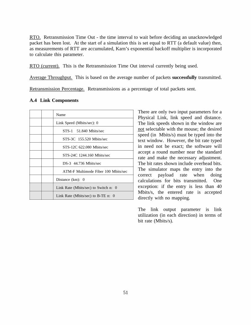
RTO. Retransmission Time Out - the time interval to wait before deciding an unacknowledgedpacket has been lost. At the start of a simulation this is set equal to RTT (a default value) then,as measurements of RTT are accumulated, Karn’s exponential backoff multiplier is incorporatedto calculate this parameter.

RTO (current). This is the Retransmission Time Out interval currently being used.

Average Throughput.This is based on the average number of packetssuccessfullytransmitted.

Retransmission Percentage.Retransmissions as a percentage of total packets sent.

A.4 Link Components

There are only two input parameters for aName

Link Speed (Mbits/sec): 0

STS-1 51.840 Mbits/sec

STS-3C 155.520 Mbits/sec

STS-12C 622.080 Mbits/sec

STS-24C 1244.160 Mbits/sec

DS-3 44.736 Mbits/sec

ATM-F Multimode Fiber 100 Mbits/sec

Distance (km): 0

Link Rate (Mbits/sec) to Switch n: 0

Link Rate (Mbits/sec) to B-TE n: 0

Physical Link, link speed and distance.The link speeds shown in the window arenot selectable with the mouse; the desiredspeed (in Mbits/s) must be typed into thetext window. However, the bit rate typedin need not be exact; the software willaccept a round number near the standardrate and make the necessary adjustment.The bit rates shown include overhead bits.The simulator maps the entry into thecorrect payload rate when doingcalculations for bits transmitted. Oneexception: if the entry is less than 40Mbits/s, the entered rate is accepteddirectly with no mapping.

The link output parameter is linkutilization (in each direction) in terms ofbit rate (Mbits/s).

51

52

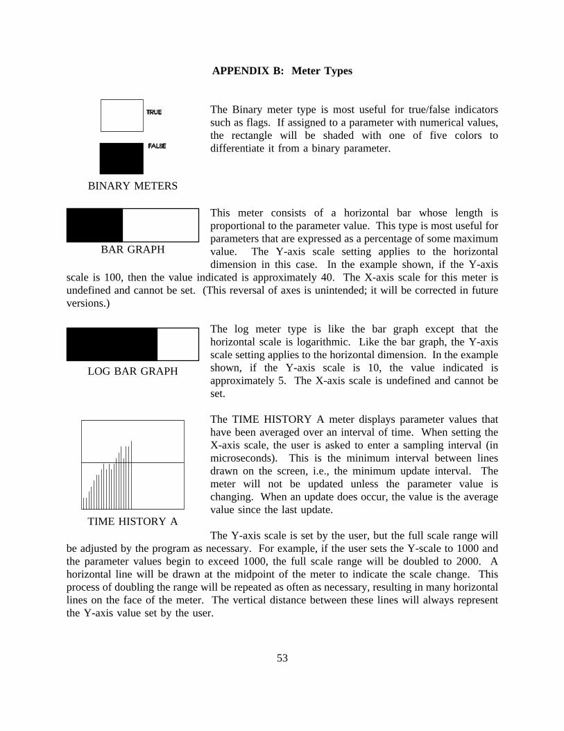
APPENDIX B: Meter Types

BINARY METERS

The Binary meter type is most useful for true/false indicatorssuch as flags. If assigned to a parameter with numerical values,the rectangle will be shaded with one of five colors todifferentiate it from a binary parameter.

This meter consists of a horizontal bar whose length is

BAR GRAPH

proportional to the parameter value. This type is most useful forparameters that are expressed as a percentage of some maximumvalue. The Y-axis scale setting applies to the horizontaldimension in this case. In the example shown, if the Y-axis

scale is 100, then the value indicated is approximately 40. The X-axis scale for this meter isundefined and cannot be set. (This reversal of axes is unintended; it will be corrected in futureversions.)

The log meter type is like the bar graph except that the

LOG BAR GRAPH

horizontal scale is logarithmic. Like the bar graph, the Y-axisscale setting applies to the horizontal dimension. In the exampleshown, if the Y-axis scale is 10, the value indicated isapproximately 5. The X-axis scale is undefined and cannot beset.

The TIME HISTORY A meter displays parameter values that

TIME HISTORY A

have been averaged over an interval of time. When setting theX-axis scale, the user is asked to enter a sampling interval (inmicroseconds). This is the minimum interval between linesdrawn on the screen, i.e., the minimum update interval. Themeter will not be updated unless the parameter value ischanging. When an update does occur, the value is the averagevalue since the last update.

The Y-axis scale is set by the user, but the full scale range willbe adjusted by the program as necessary. For example, if the user sets the Y-scale to 1000 andthe parameter values begin to exceed 1000, the full scale range will be doubled to 2000. Ahorizontal line will be drawn at the midpoint of the meter to indicate the scale change. Thisprocess of doubling the range will be repeated as often as necessary, resulting in many horizontallines on the face of the meter. The vertical distance between these lines will always representthe Y-axis value set by the user.

53

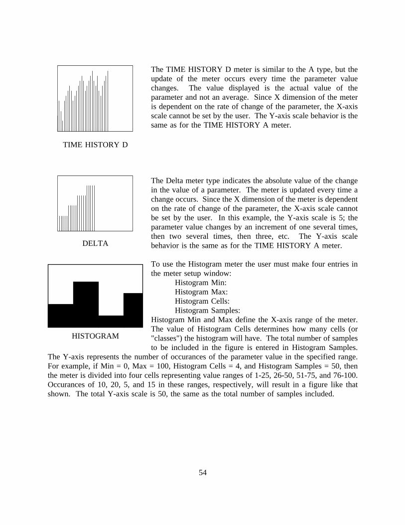
TIME HISTORY D

The TIME HISTORY D meter is similar to the A type, but theupdate of the meter occurs every time the parameter valuechanges. The value displayed is the actual value of theparameter and not an average. Since X dimension of the meteris dependent on the rate of change of the parameter, the X-axisscale cannot be set by the user. The Y-axis scale behavior is thesame as for the TIME HISTORY A meter.

DELTA

The Delta meter type indicates the absolute value of the changein the value of a parameter. The meter is updated every time achange occurs. Since the X dimension of the meter is dependenton the rate of change of the parameter, the X-axis scale cannotbe set by the user. In this example, the Y-axis scale is 5; theparameter value changes by an increment of one several times,then two several times, then three, etc. The Y-axis scalebehavior is the same as for the TIME HISTORY A meter.

To use the Histogram meter the user must make four entries in

HISTOGRAM

the meter setup window:Histogram Min:Histogram Max:Histogram Cells:Histogram Samples:

Histogram Min and Max define the X-axis range of the meter.The value of Histogram Cells determines how many cells (or"classes") the histogram will have. The total number of samplesto be included in the figure is entered in Histogram Samples.

The Y-axis represents the number of occurances of the parameter value in the specified range.For example, if Min = 0, Max = 100, Histogram Cells = 4, and Histogram Samples = 50, thenthe meter is divided into four cells representing value ranges of 1-25, 26-50, 51-75, and 76-100.Occurances of 10, 20, 5, and 15 in these ranges, respectively, will result in a figure like thatshown. The total Y-axis scale is 50, the same as the total number of samples included.

54

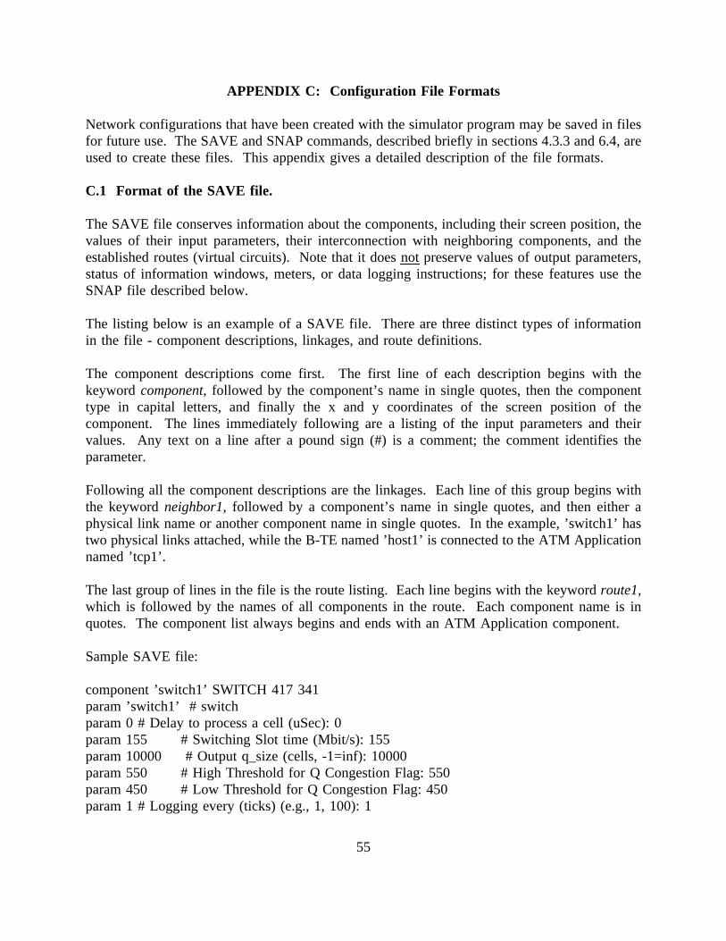
APPENDIX C: Configuration File Formats

Network configurations that have been created with the simulator program may be saved in filesfor future use. The SAVE and SNAP commands, described briefly in sections 4.3.3 and 6.4, areused to create these files. This appendix gives a detailed description of the file formats.

C.1 Format of the SAVE file.

The SAVE file conserves information about the components, including their screen position, thevalues of their input parameters, their interconnection with neighboring components, and theestablished routes (virtual circuits). Note that it does notpreserve values of output parameters,status of information windows, meters, or data logging instructions; for these features use theSNAP file described below.

The listing below is an example of a SAVE file. There are three distinct types of informationin the file - component descriptions, linkages, and route definitions.

The component descriptions come first. The first line of each description begins with thekeyword component, followed by the component’s name in single quotes, then the componenttype in capital letters, and finally the x and y coordinates of the screen position of thecomponent. The lines immediately following are a listing of the input parameters and theirvalues. Any text on a line after a pound sign (#) is a comment; the comment identifies theparameter.

Following all the component descriptions are the linkages. Each line of this group begins withthe keywordneighbor1, followed by a component’s name in single quotes, and then either aphysical link name or another component name in single quotes. In the example, ’switch1’ hastwo physical links attached, while the B-TE named ’host1’ is connected to the ATM Applicationnamed ’tcp1’.

The last group of lines in the file is the route listing. Each line begins with the keywordroute1,which is followed by the names of all components in the route. Each component name is inquotes. The component list always begins and ends with an ATM Application component.

Sample SAVE file:

component ’switch1’ SWITCH 417 341param ’switch1’ # switchparam 0 # Delay to process a cell (uSec): 0param 155 # Switching Slot time (Mbit/s): 155param 10000 # Output q_size (cells, -1=inf): 10000param 550 # High Threshold for Q Congestion Flag: 550param 450 # Low Threshold for Q Congestion Flag: 450param 1 # Logging every (ticks) (e.g., 1, 100): 1

55

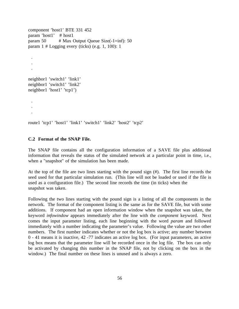
component ’host1’ BTE 331 452param ’host1’ # host1param 50 # Max Output Queue Size(-1=inf): 50param 1 # Logging every (ticks) (e.g. 1, 100): 1

.

.

.

neighbor1 ’switch1’ ’link1’neighbor1 ’switch1’ ’link2’neighbor1 ’host1’ ’tcp1’)

.

.

.

route1 ’tcp1’ ’host1’ ’link1’ ’switch1’ ’link2’ ’host2’ ’tcp2’

C.2 Format of the SNAP File.

The SNAP file contains all the configuration information of a SAVE file plus additionalinformation that reveals the status of the simulated network at a particular point in time, i.e.,when a "snapshot" of the simulation has been made.

At the top of the file are two lines starting with the pound sign (#). The first line records theseed used for that particular simulation run. (This line will not be loaded or used if the file isused as a configuration file.) The second line records the time (in ticks) when thesnapshot was taken.

Following the two lines starting with the pound sign is a listing of all the components in thenetwork. The format of the component listing is the same as for the SAVE file, but with someadditions. If component had an open information window when the snapshot was taken, thekeyword infowindow appears immediately after the line with thecomponentkeyword. Nextcomes the input parameter listing, each line beginning with the wordparam and followedimmediately with a number indicating the parameter’s value. Following the value are two othernumbers. The first number indicates whether or not the log box is active; any number between0 - 41 means it is inactive, 42 -77 indicates an active log box. (For input parameters, an activelog box means that the parameter line will be recorded once in the log file. The box can onlybe activated by changing this number in the SNAP file, not by clicking on the box in thewindow.) The final number on these lines is unused and is always a zero.

56

Following theparamlines is a list of all output parameters, each line beginning with the keywordpflags. The text on each of these lines following the pound sign is a comment that contains theparameter description and value. (Output parameter values are not used when the SNAP file isused as a configuration file.)

On each output parameter line, following thepflagskeyword, there is a 2 or a 4 with the letter’a’ or ’b’ appended. This is a code that reveals whether the output parameter has its data loggingbox in the active mode, and/or its meter window open. The different combinations are asfollows:

2a = the log box is not active, the meter window is closed.2b = the log box is active, the meter window is closed.4a = the log box is inactive, the meter window is open.4b = the log box is active, the meter window in open.

Following the above is another entry consisting of a single digit with the value of 1 through 7.This digit represents the type of meter used for the graphical display. The types are identifiedas follows:

1 = Binary meter2 = Bar graph3 = Log graph4 = time history A5 = time history D6 = Delta meter7 = Histogram

If the meter window for an output parameter is open, the coordinates of its position on the screenand its dimensions are given immediately following the meter type entry. For example, for theline pflags 2b 4 562 424 159 93, the x and y coordinates of the window are 562 and 424, and159 and 93 are the height and width, respectively.

The remainder of the SNAP file contains linkage and route definition; these are in a formatidentical to the SAVE file.

Sample SNAP file:

# Seed 776093072# Time of snapshot (ticks) 0component ’switch1’ SWITCH 417 341infowindowparam ’switch1’ 32 0 # switch1param 0 12 0 # Delay to process a cell (uSec): 0

57

param 155 12 0 # Switching Slot time (Mbit/s): 155param 10000 12 0 # Output q_size (cells, -1=inf): 10000param 550 12 0 # High Threshold for Q Congestion Flag: 550param 450 12 0 # Low Threshold for Q Congestion Flag: 450param 1 12 0 # Logging every (ticks) (e.g. 1, 100): 1pflags 2a 4 #Cells Received: 0pflags 2a 4 #Cell Drop %: 0pflags 2a 4 #Cells in VBR Q to link1: 0pflags 2a 4 #Cells dropped in VBR Q to link1: 0pflags 2a 4 #Cells in ABR Q to link1: 0pflags 2a 4 #Cells Dropped in ABR Q to link1: 0pflags 2a 1 #Congestion for Link link1: FALSEpflags 2a 4 #Cells in VBR Q to link2: 0pflags 2a 4 #Cells dropped in VBR Q to link2: 0pflags 2a 4 #Cells in ABR Q to link2: 0pflags 2a 4 #Cells Dropped in ABR Q to link2: 0pflags 2a 1 #Congestion for Link link2: FALSE

component ’host2’ BTE 562 460param ’host2’ 32 0 # host2param 50 12 0 # Max Output Queue Size(-1=inf): 50param 1 12 0 # Logging every (ticks) (e.g. 1, 100): 1pflags 2b 4 562 424 159 93 #Cells Received: 0pflags 2a 4 #Cells in VBR Q to link2: 0pflags 2a 4 #Cells dropped in VBR Q to link2: 0pflags 2a 4 #Cells in ABR Q to link2: 0pflags 4b 1 446 547 130 55 #Cells Dropped in ABR Q to link2:

58