The Mutation Game, Coxeter Graphs, andPartially Ordered Multisets

N. J. Wildberger∗

Introduction

The Mutation Game

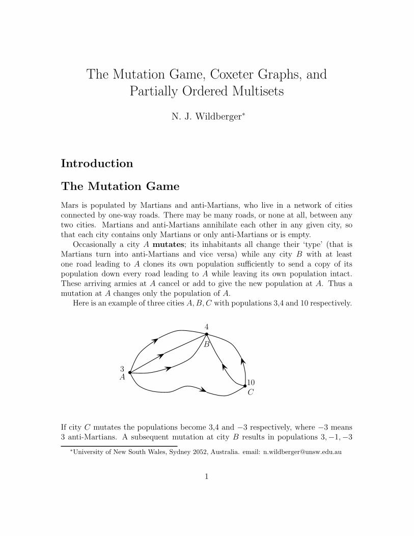
Mars is populated by Martians and anti-Martians, who live in a network of citiesconnected by one-way roads. There may be many roads, or none at all, between anytwo cities. Martians and anti-Martians annihilate each other in any given city, sothat each city contains only Martians or only anti-Martians or is empty.

Occasionally a city A mutates; its inhabitants all change their ‘type’ (that isMartians turn into anti-Martians and vice versa) while any city B with at leastone road leading to A clones its own population sufficiently to send a copy of itspopulation down every road leading to A while leaving its own population intact.These arriving armies at A cancel or add to give the new population at A. Thus amutation at A changes only the population of A.

Here is an example of three cities A,B,C with populations 3,4 and 10 respectively.

3A

•

4

B

•

10C

•

If city C mutates the populations become 3,4 and −3 respectively, where −3 means3 anti-Martians. A subsequent mutation at city B results in populations 3,−1,−3

∗University of New South Wales, Sydney 2052, Australia. email: n.wildberger@unsw.edu.au

1

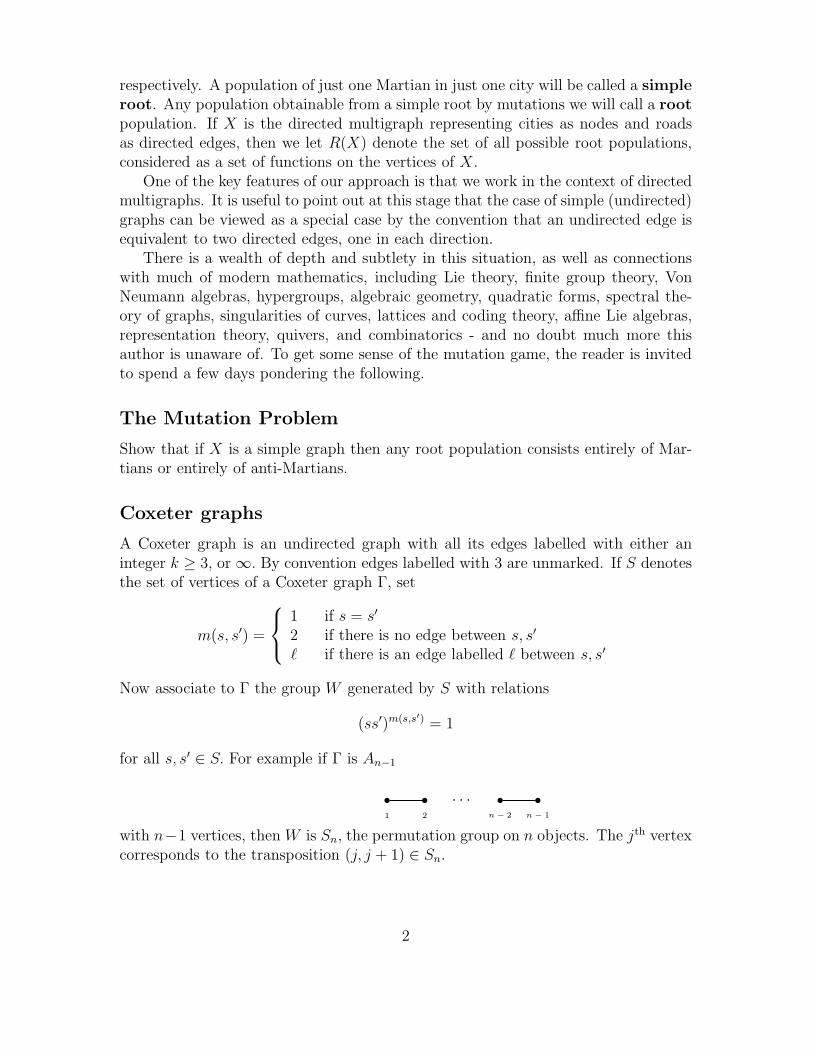
respectively. A population of just one Martian in just one city will be called a simpleroot. Any population obtainable from a simple root by mutations we will call a rootpopulation. If X is the directed multigraph representing cities as nodes and roadsas directed edges, then we let R(X) denote the set of all possible root populations,considered as a set of functions on the vertices of X.

One of the key features of our approach is that we work in the context of directedmultigraphs. It is useful to point out at this stage that the case of simple (undirected)graphs can be viewed as a special case by the convention that an undirected edge isequivalent to two directed edges, one in each direction.

There is a wealth of depth and subtlety in this situation, as well as connectionswith much of modern mathematics, including Lie theory, finite group theory, VonNeumann algebras, hypergroups, algebraic geometry, quadratic forms, spectral the-ory of graphs, singularities of curves, lattices and coding theory, affine Lie algebras,representation theory, quivers, and combinatorics - and no doubt much more thisauthor is unaware of. To get some sense of the mutation game, the reader is invitedto spend a few days pondering the following.

The Mutation Problem

Show that if X is a simple graph then any root population consists entirely of Mar-tians or entirely of anti-Martians.

Coxeter graphs

A Coxeter graph is an undirected graph with all its edges labelled with either aninteger k ≥ 3, or ∞. By convention edges labelled with 3 are unmarked. If S denotesthe set of vertices of a Coxeter graph Γ, set

m(s, s′) =

⎧⎨⎩

1 if s = s′

2 if there is no edge between s, s′

� if there is an edge labelled � between s, s′

Now associate to Γ the group W generated by S with relations

(ss′)m(s,s′) = 1

for all s, s′ ∈ S. For example if Γ is An−1

· · ·1 2 n − 2 n − 1

with n−1 vertices, then W is Sn, the permutation group on n objects. The jth vertexcorresponds to the transposition (j, j + 1) ∈ Sn.

2

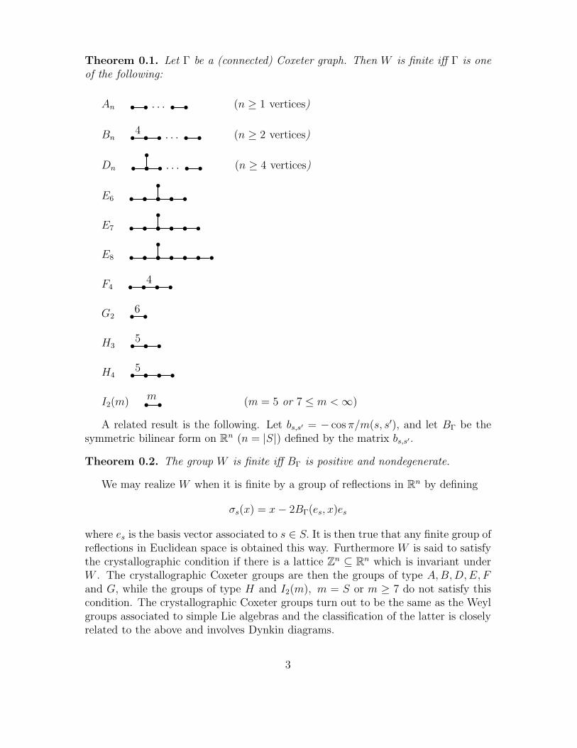
Theorem 0.1. Let Γ be a (connected) Coxeter graph. Then W is finite iff Γ is oneof the following:

An · · · (n ≥ 1 vertices)

Bn · · ·4 (n ≥ 2 vertices)

Dn · · · (n ≥ 4 vertices)

E6

E7

E8

F44

G26

H35

H45

I2(m)m

(m = 5 or 7 ≤ m <∞)

A related result is the following. Let bs,s′ = − cosπ/m(s, s′), and let BΓ be thesymmetric bilinear form on Rn (n = |S|) defined by the matrix bs,s′.

Theorem 0.2. The group W is finite iff BΓ is positive and nondegenerate.

We may realize W when it is finite by a group of reflections in Rn by defining

σs(x) = x− 2BΓ(es, x)es

where es is the basis vector associated to s ∈ S. It is then true that any finite group ofreflections in Euclidean space is obtained this way. Furthermore W is said to satisfythe crystallographic condition if there is a lattice Zn ⊆ Rn which is invariant underW . The crystallographic Coxeter groups are then the groups of type A,B,D,E, Fand G, while the groups of type H and I2(m), m = S or m ≥ 7 do not satisfy thiscondition. The crystallographic Coxeter groups turn out to be the same as the Weylgroups associated to simple Lie algebras and the classification of the latter is closelyrelated to the above and involves Dynkin diagrams.

3

Before explaining this connection, let us point out that when the Coxeter graphis of type ADE, all edges have label 3, the elements bs,s′ are either 0, 1 or −1

2, so the

form BΓ is essentially integral (by multiplying it by 2). However for the other cases

BΓ has terms like −√

22, −1+

√5

4so is not integral.

Root systems and Dynkin diagrams

Let E be a Euclidean space, by which we mean a finite dimensional real vector spacewith a Euclidean inner product (, ). A root system R ⊂ E is a subset such that

1. R is finite, 0 �∈ R and span (R) = E

2. ∀α ∈ R the reflection sα defined by

xsα = x− 2(x, α)α

(α, α)

sends R to R

3. ∀α, β ∈ R, βsα − β is an integer multiple of α.

The root system is called reduced if R ∪ Rα = {α,−α} for all α ∈ R. Theassociated Weyl group is the subgroup W of GL(E) generated by the reflectionssα, α ∈ R. The rank of R is the dimension of E.

Here are the rank 2 reduced root systems:

A1 × A1 A2

B2 G2

4

Let R be a reduced root system. Then it is always possible to find a basis S ⊂ Rof E with the property that every element of R is a linear combination of elements ofS with either all coefficients non-negative or all coefficients non-positive. Associatedto such a choice S of simple roots is the Cartan matrix (n(α, β))α,β∈S where

n(α, β) = 2(α, β)

(β, β)∈ Z,

and the Dynkin diagram constructed as follows. Draw a vertex for each s ∈ S.Connect i and j with

i) a simple edge if n(i, j) = n(j, i) = −1 ie.i j

ii) a directed double edge from j to i if 2n(i, j) = n(j, i) = −2 ie.i j

� �

iii) a directed triple edge from j to i if 3n(i, j) = n(j, i) = −3 ie.i j� �

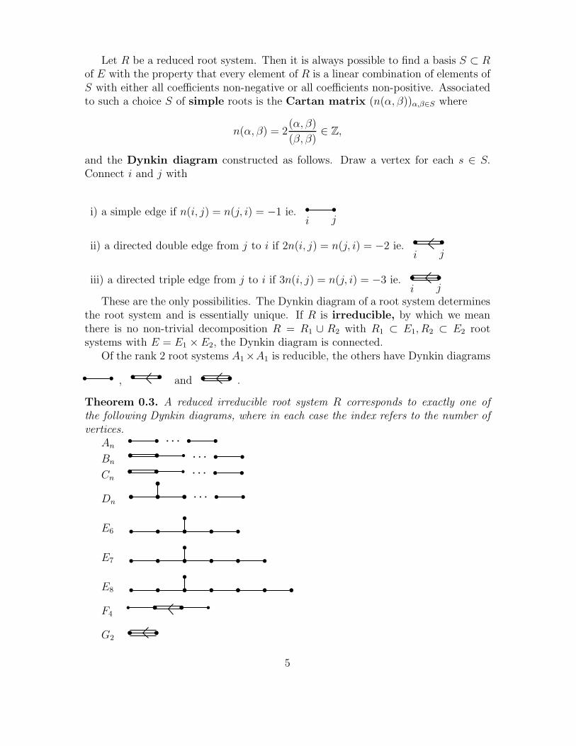
These are the only possibilities. The Dynkin diagram of a root system determinesthe root system and is essentially unique. If R is irreducible, by which we meanthere is no non-trivial decomposition R = R1 ∪ R2 with R1 ⊂ E1, R2 ⊂ E2 rootsystems with E = E1 ×E2, the Dynkin diagram is connected.

Of the rank 2 root systems A1×A1 is reducible, the others have Dynkin diagrams

,� �

and � � .

Theorem 0.3. A reduced irreducible root system R corresponds to exactly one ofthe following Dynkin diagrams, where in each case the index refers to the number ofvertices.

An� � �

Bn� �

� � �

Cn� �

� � �

Dn� �

�

� � � �

E6

E7

E8

F4� �

G2� �

5

This classification arose historically through the connection with simple Lie alge-bras. Each such Lie algebra has associated to it a root system and the above theoremis a key ingredient in showing that simple Lie algebras are classified by the same listof Dynkin diagrams.

Note that by replacing Dynkin type bonds� �

and � � with the cor-

responding Coxeter type bonds 4 , 6 we get a subset of the Coxetergraphs of Theorem ?? in fact exactly the crystallographic Coxeter graphs. This is areflection of the fact that Weyl groups and crystallographic Coxeter groups coincide.

Directed Multigraphs

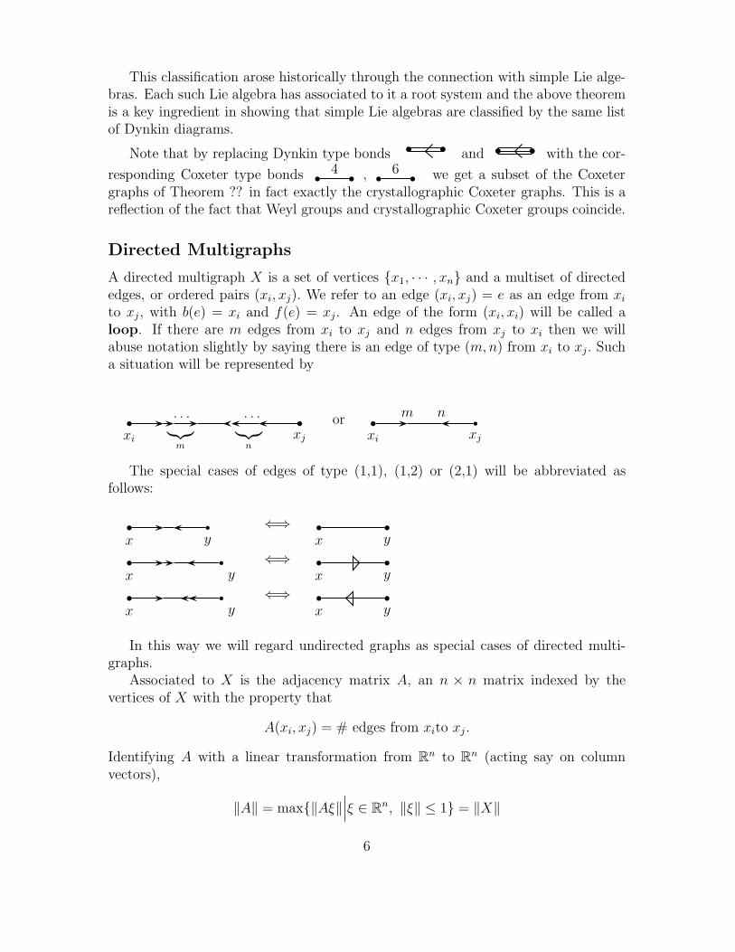
A directed multigraph X is a set of vertices {x1, · · · , xn} and a multiset of directededges, or ordered pairs (xi, xj). We refer to an edge (xi, xj) = e as an edge from xito xj , with b(e) = xi and f(e) = xj . An edge of the form (xi, xi) will be called aloop. If there are m edges from xi to xj and n edges from xj to xi then we willabuse notation slightly by saying there is an edge of type (m,n) from xi to xj . Sucha situation will be represented by

. . .

xi xj

. . .︸︷︷︸m

︸︷︷︸n

or m n

xi xj

The special cases of edges of type (1,1), (1,2) or (2,1) will be abbreviated asfollows:

x y⇐⇒

x y

x y⇐⇒

x y

x y⇐⇒

x y

In this way we will regard undirected graphs as special cases of directed multi-graphs.

Associated to X is the adjacency matrix A, an n × n matrix indexed by thevertices of X with the property that

A(xi, xj) = # edges from xito xj .

Identifying A with a linear transformation from Rn to Rn (acting say on columnvectors),

‖A‖ = max{‖Aξ‖∣∣∣ξ ∈ Rn, ‖ξ‖ ≤ 1} = ‖X‖

6

is the operator norm of A, and by definition the norm of X. If the eigenvalues of Aare λ1, · · · , λn ∈ C possibly with multiplicity, then

sp(A) = max{|λi|∣∣i = 1, · · · , n} = sp(X)

is the spectral radius of A, and by definition the spectral radius ofX. For symmetricmatrices ‖A‖ = sp(A) but in general sp(A) ≤ ‖A‖.

For undirected graphs, the classification of those X for which ‖X‖ = 2 or ‖X‖ <2 are well known (see [?]). We are here interested in the more general questionof classifying those directed multigraphs X for which sp(X) = 2 and sp(X) < 2,especially in the case when X has no loops and is bi-directed, meaning for all i, jA(xi, xj) > 0 implies A(xj , xi) > 0.

A square n×n matrix A is irreducible iff for each i, j ∈ {1, · · · , n} there exists aninteger p (depending on i and j) such that Ap(i, j) > 0. If A has non-negative entries,a Perron-Frobenious vector for A is an eigenvector ξ ∈ Rn of A with non-negativeentries. If A,B are matrices, we define A ≤ B iff B − A has non-negative entries.Here is the fundamental tool one needs in this subject.

Theorem 0.4 (Perron-Frobenius). Let A be an irreducible non-negative n × nmatrix. Then

i) a Perron-Frobenius vector ξ exists and is unique up to multiplication by a pos-itive scalar.

ii) ξ corresponds to a simple eigenvalue λ which is the spectral radius of A.

iii) if A′ is a second non-negative n × n matrix with A′ ≤ A and A′ �= A, thensp(A′) < sp(A).

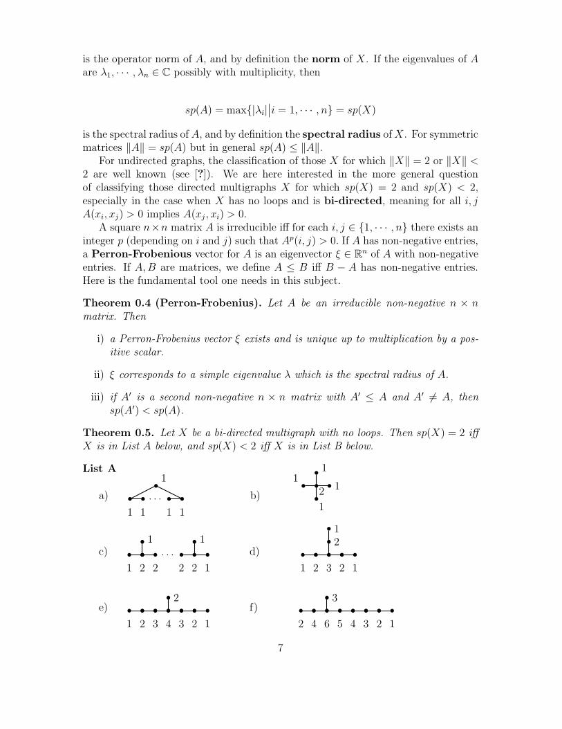
Theorem 0.5. Let X be a bi-directed multigraph with no loops. Then sp(X) = 2 iffX is in List A below, and sp(X) < 2 iff X is in List B below.

List A

a) . . .

1 1 1 1

1

b)

11

2 1

1

c) . . .

1 2 2

1 1

2 2 1

d)

1 2 3 2 1

21

e)

1 2 3 4 3 2 1

2f)

2 4 6 5 4 3 2 1

3

7

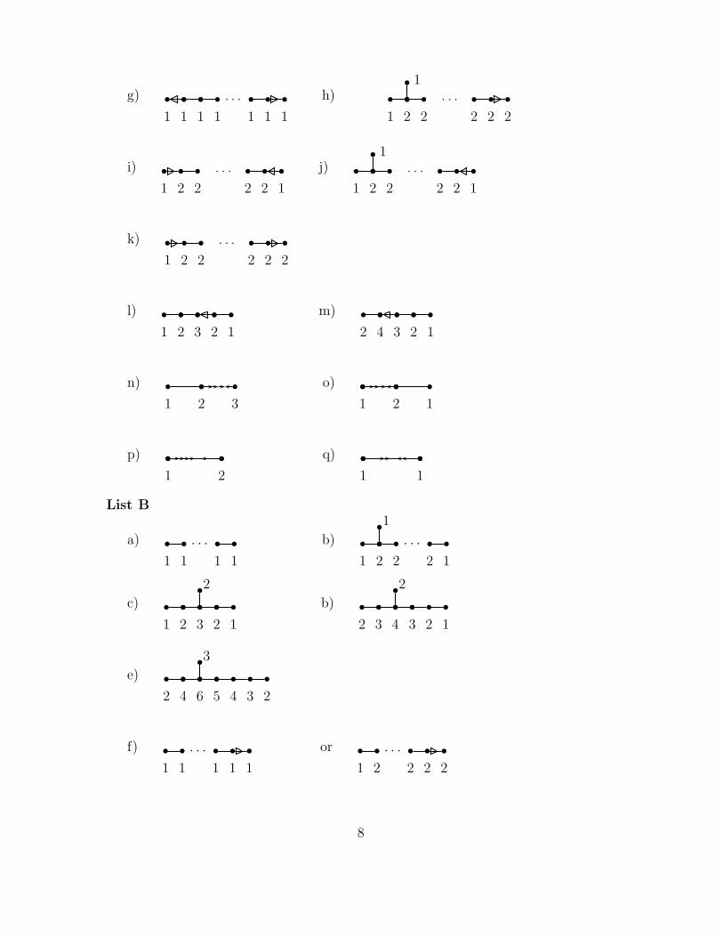
g)

1 1 1 1

. . .

1 1 1

h) . . .

2 2 21 2 2

1

i) . . .

2 2 11 2 2

j) . . .

2 2 11 2 2

1

k) . . .

2 2 21 2 2

l)

1 2 3 2 1

m)

2 4 3 2 1

n)

1 2 3

o)

1 2 1

p)

1 2

q)

1 1

List B

a) · · ·1 1 1 1

b) · · ·1 2 2 2 1

1

c)

1 2 3 2 1

2

b)

2 3 4 3 2 1

2

e)

2 4 6 5 4 3 2

3

f) · · ·1 1 1 1 1

or · · ·1 2 2 2 2

8

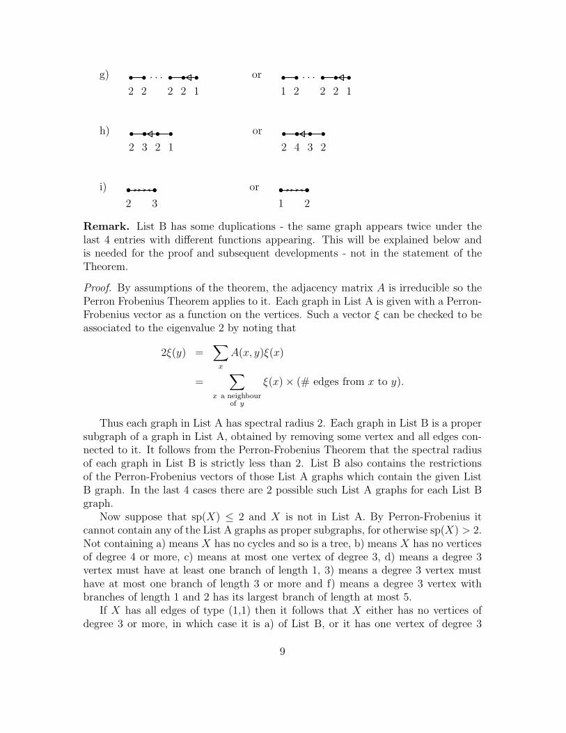
g) · · ·2 2 2 2 1

or · · ·1 2 2 2 1

h)

2 3 2 1

or

2 4 3 2

i)

2 3

or

1 2

Remark. List B has some duplications - the same graph appears twice under thelast 4 entries with different functions appearing. This will be explained below andis needed for the proof and subsequent developments - not in the statement of theTheorem.

Proof. By assumptions of the theorem, the adjacency matrix A is irreducible so thePerron Frobenius Theorem applies to it. Each graph in List A is given with a Perron-Frobenius vector as a function on the vertices. Such a vector ξ can be checked to beassociated to the eigenvalue 2 by noting that

2ξ(y) =∑x

A(x, y)ξ(x)

=∑

x a neighbourof y

ξ(x) × (# edges from x to y).

Thus each graph in List A has spectral radius 2. Each graph in List B is a propersubgraph of a graph in List A, obtained by removing some vertex and all edges con-nected to it. It follows from the Perron-Frobenius Theorem that the spectral radiusof each graph in List B is strictly less than 2. List B also contains the restrictionsof the Perron-Frobenius vectors of those List A graphs which contain the given ListB graph. In the last 4 cases there are 2 possible such List A graphs for each List Bgraph.

Now suppose that sp(X) ≤ 2 and X is not in List A. By Perron-Frobenius itcannot contain any of the List A graphs as proper subgraphs, for otherwise sp(X) > 2.Not containing a) means X has no cycles and so is a tree, b) means X has no verticesof degree 4 or more, c) means at most one vertex of degree 3, d) means a degree 3vertex must have at least one branch of length 1, 3) means a degree 3 vertex musthave at most one branch of length 3 or more and f) means a degree 3 vertex withbranches of length 1 and 2 has its largest branch of length at most 5.

If X has all edges of type (1,1) then it follows that X either has no vertices ofdegree 3 or more, in which case it is a) of List B, or it has one vertex of degree 3

9

with two branches of length 1 in which case it is b) of List B, or it has one vertex ofdegree 3 with branches of length 1 and 2 and the other of lengths 2,3 or 4, giving c)d) or e) of List B.

X can have at most one edge not of type (1,1), for otherwise we could find apath between the two edges giving a subgraph of type either g) i) or k) of List A. Sosuppose X has exactly one edge not of type (1,1), say joining x and y. Then h) andj) of List A show that X contains no vertex of degree 3 or more. Furthermore p) andq) of List A show that the edge between x and y must be of type (1,3) or (3,1) orless, and if it is of type (1,3) or (3,1) then n) and p of List A show it must be i) ofList B. If neither x and y are endpoints then l) and m) of List A show that X mustbe h) of List B. If x or y are endpoints the only remaining possibilities are f) and g)in List B.

In conclusion, X must be one of the graphs of List B, and this concludes theproof.

Corollary. If X is a bidirected multigraph with no loops and sp(X) > 2 then Xcontains a List A graph as a subgraph.

Proof. The proof of the Theorem shows that sp(X) ≤ 2 and X not in List A impliesX is in List B. But in fact the same argument shows that sp(X) > 2 and X notcontaining a List A graph implies X is in List B, which is impossible by the Theorem.

Mutation-reflections on directed multigraphs

Let X be a directed multigraph, perhaps not connected. Let P (X) denote the set ofintegral valued functions on the vertices of X, with P+(X) and P−(X) respectivelythe subsets of non-negative and non-positive functions. For each vertex x, we definea map sx : P (X) → P (X) by

(psx)(y) =

⎧⎨⎩

p(y) if y �= x

−p(x) +∑z �=x

A(z, x)p(z) if y = x

which we call the mutation, or reflection at x.

Theorem 0.6. If x and y are vertices of X then

i) s2x = identity

ii) sxsy = sysx if x and y are not neighbours

iii) sxsy has finite order greater than 2 iff the edge type of (x, y) is a) (1,1) b) (1,2)or (2,1) or c) (1,3) or (3,1) in which case sxsy has order a) 3 b) 4 or c) 6respectively.

10

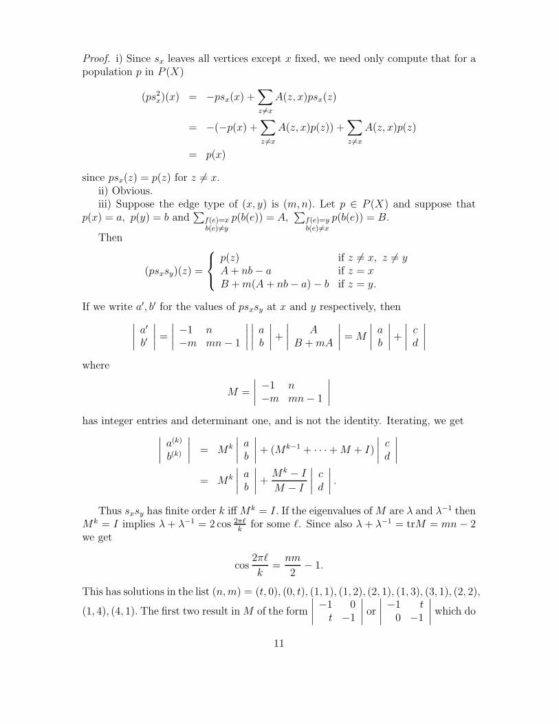
Proof. i) Since sx leaves all vertices except x fixed, we need only compute that for apopulation p in P (X)

(ps2x)(x) = −psx(x) +

∑z �=x

A(z, x)psx(z)

= −(−p(x) +∑z �=x

A(z, x)p(z)) +∑z �=x

A(z, x)p(z)

= p(x)

since psx(z) = p(z) for z �= x.ii) Obvious.iii) Suppose the edge type of (x, y) is (m,n). Let p ∈ P (X) and suppose that

p(x) = a, p(y) = b and∑

f(e)=xb(e)�=y

p(b(e)) = A,∑

f(e)=yb(e)�=x

p(b(e)) = B.

Then

(psxsy)(z) =

⎧⎨⎩

p(z) if z �= x, z �= yA+ nb− a if z = xB +m(A + nb− a) − b if z = y.

If we write a′, b′ for the values of psxsy at x and y respectively, then∣∣∣∣ a′b′∣∣∣∣ =

∣∣∣∣ −1 n−m mn− 1

∣∣∣∣∣∣∣∣ ab

∣∣∣∣ +

∣∣∣∣ AB +mA

∣∣∣∣ = M

∣∣∣∣ ab∣∣∣∣ +

∣∣∣∣ cd∣∣∣∣

where

M =

∣∣∣∣ −1 n−m mn− 1

∣∣∣∣has integer entries and determinant one, and is not the identity. Iterating, we get∣∣∣∣ a(k)

b(k)

∣∣∣∣ = Mk

∣∣∣∣ ab∣∣∣∣ + (Mk−1 + · · · +M + I)

∣∣∣∣ cd∣∣∣∣

= Mk

∣∣∣∣ ab∣∣∣∣ +

Mk − I

M − I

∣∣∣∣ cd∣∣∣∣ .

Thus sxsy has finite order k iff Mk = I. If the eigenvalues of M are λ and λ−1 thenMk = I implies λ+ λ−1 = 2 cos 2π�

kfor some �. Since also λ + λ−1 = trM = mn− 2

we get

cos2π�

k=nm

2− 1.

This has solutions in the list (n,m) = (t, 0), (0, t), (1, 1), (1, 2), (2, 1), (1, 3), (3, 1), (2, 2),

(1, 4), (4, 1). The first two result in M of the form

∣∣∣∣ −1 0t −1

∣∣∣∣ or

∣∣∣∣ −1 t0 −1

∣∣∣∣ which do

11

not have finite order, and the last three giveM to be one of

∣∣∣∣ −1 2−2 3

∣∣∣∣ ,∣∣∣∣ −1 4−1 3

∣∣∣∣ ,∣∣∣∣ −1 1−4 3

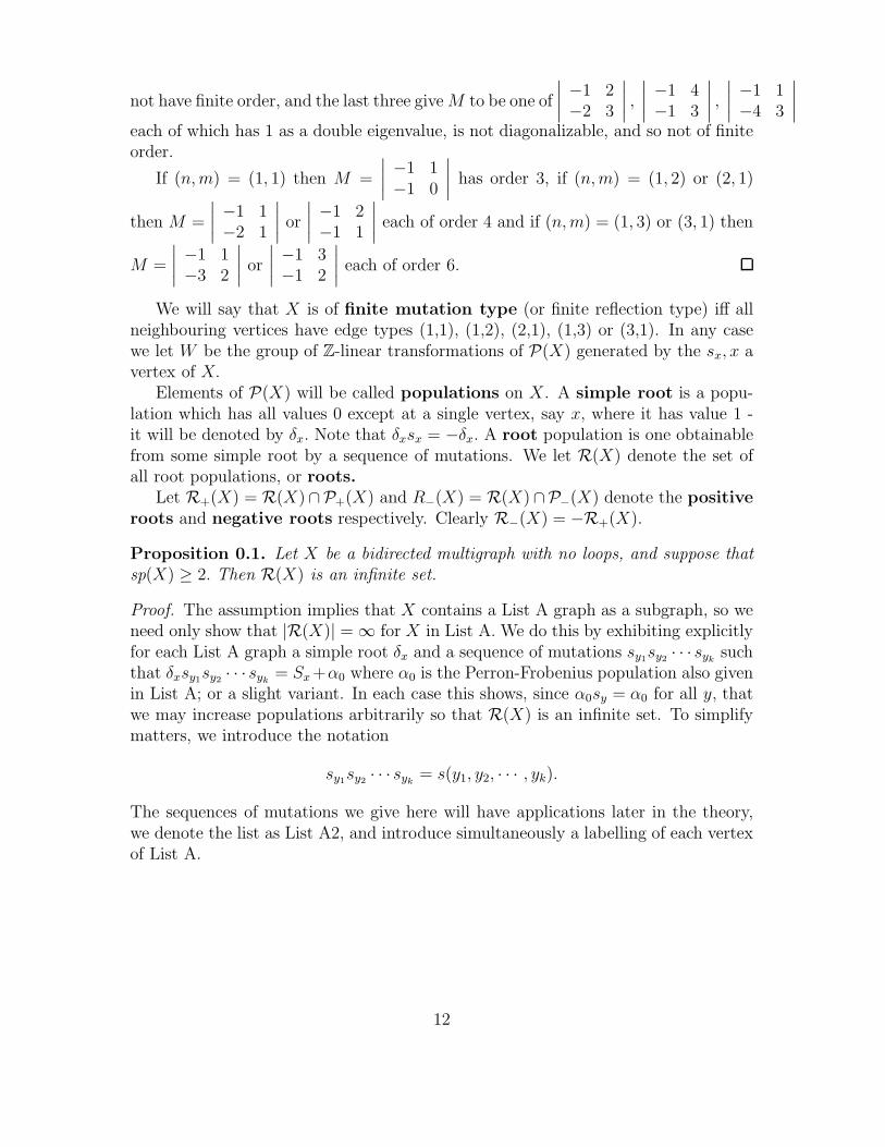
∣∣∣∣each of which has 1 as a double eigenvalue, is not diagonalizable, and so not of finiteorder.

If (n,m) = (1, 1) then M =

∣∣∣∣ −1 1−1 0

∣∣∣∣ has order 3, if (n,m) = (1, 2) or (2, 1)

then M =

∣∣∣∣ −1 1−2 1

∣∣∣∣ or

∣∣∣∣ −1 2−1 1

∣∣∣∣ each of order 4 and if (n,m) = (1, 3) or (3, 1) then

M =

∣∣∣∣ −1 1−3 2

∣∣∣∣ or

∣∣∣∣ −1 3−1 2

∣∣∣∣ each of order 6.

We will say that X is of finite mutation type (or finite reflection type) iff allneighbouring vertices have edge types (1,1), (1,2), (2,1), (1,3) or (3,1). In any casewe let W be the group of Z-linear transformations of P(X) generated by the sx, x avertex of X.

Elements of P(X) will be called populations on X. A simple root is a popu-lation which has all values 0 except at a single vertex, say x, where it has value 1 -it will be denoted by δx. Note that δxsx = −δx. A root population is one obtainablefrom some simple root by a sequence of mutations. We let R(X) denote the set ofall root populations, or roots.

Let R+(X) = R(X)∩P+(X) and R−(X) = R(X)∩P−(X) denote the positiveroots and negative roots respectively. Clearly R−(X) = −R+(X).

Proposition 0.1. Let X be a bidirected multigraph with no loops, and suppose thatsp(X) ≥ 2. Then R(X) is an infinite set.

Proof. The assumption implies that X contains a List A graph as a subgraph, so weneed only show that |R(X)| = ∞ for X in List A. We do this by exhibiting explicitlyfor each List A graph a simple root δx and a sequence of mutations sy1sy2 · · · syk

suchthat δxsy1sy2 · · · syk

= Sx+α0 where α0 is the Perron-Frobenius population also givenin List A; or a slight variant. In each case this shows, since α0sy = α0 for all y, thatwe may increase populations arbitrarily so that R(X) is an infinite set. To simplifymatters, we introduce the notation

sy1sy2 · · · syk= s(y1, y2, · · · , yk).

The sequences of mutations we give here will have applications later in the theory,we denote the list as List A2, and introduce simultaneously a labelling of each vertexof List A.

12

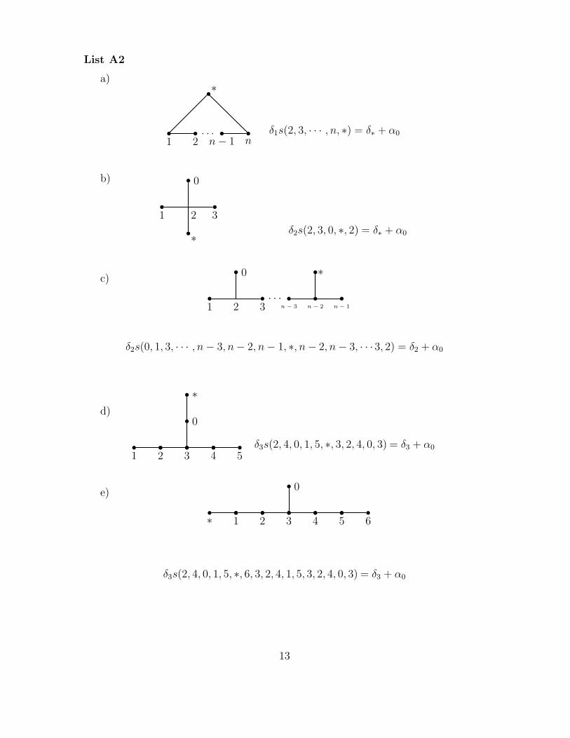
List A2

a)

. . .1 2 n− 1 n

∗

δ1s(2, 3, · · · , n, ∗) = δ∗ + α0

b) 0

31 2

∗ δ2s(2, 3, 0, ∗, 2) = δ∗ + α0

c)

1 2 3

0

· · ·n − 3 n − 2 n − 1

∗

δ2s(0, 1, 3, · · · , n− 3, n− 2, n− 1, ∗, n− 2, n− 3, · · ·3, 2) = δ2 + α0

d)

1 2 3 4 5

0

∗

δ3s(2, 4, 0, 1, 5, ∗, 3, 2, 4, 0, 3) = δ3 + α0

e)

∗ 1 2 3 4 5 6

0

δ3s(2, 4, 0, 1, 5, ∗, 6, 3, 2, 4, 1, 5, 3, 2, 4, 0, 3) = δ3 + α0

13

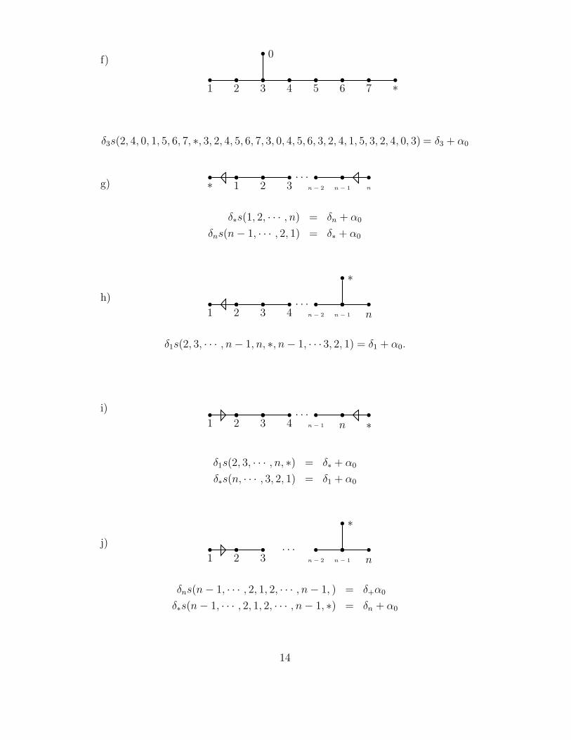
f)

1 2 3 4 5 6 7 ∗

0

δ3s(2, 4, 0, 1, 5, 6, 7, ∗, 3, 2, 4, 5, 6, 7, 3, 0, 4, 5, 6, 3, 2, 4, 1, 5, 3, 2, 4, 0, 3) = δ3 + α0

g) ∗ 1 2 3· · ·

n − 2 n − 1 n

δ∗s(1, 2, · · · , n) = δn + α0

δns(n− 1, · · · , 2, 1) = δ∗ + α0

h)

1 2 3 4· · ·

n − 2 n − 1 n

∗

δ1s(2, 3, · · · , n− 1, n, ∗, n− 1, · · · 3, 2, 1) = δ1 + α0.

i)

1 2 3 4· · ·

n − 1 n ∗

δ1s(2, 3, · · · , n, ∗) = δ∗ + α0

δ∗s(n, · · · , 3, 2, 1) = δ1 + α0

j)

1 2 3· · ·

n − 2 n − 1 n

∗

δns(n− 1, · · · , 2, 1, 2, · · · , n− 1, ) = δ+α0

δ∗s(n− 1, · · · , 2, 1, 2, · · · , n− 1, ∗) = δn + α0

14

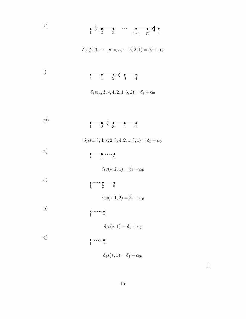
k)

1 2 3· · ·

n − 1 n ∗

δ1s(2, 3, · · · , n, ∗, n, · · ·3, 2, 1) = δ1 + α0

l)

∗ 1 2 3 4

δ2s(1, 3, ∗, 4, 2, 1, 3, 2) = δ2 + α0

m)

1 2 3 4 ∗

δ2s(1, 3, 4, ∗, 2, 3, 4, 2, 1, 3, 1) = δ2 + α0

n)

∗ 1 2

δ1s(∗, 2, 1) = δ1 + α0

o)

1 2 ∗

δ2s(∗, 1, 2) = δ2 + α0

p)

1 ∗

δ1s(∗, 1) = δ1 + α0

q)

1 ∗

δ1s(∗, 1) = δ1 + α0.

15

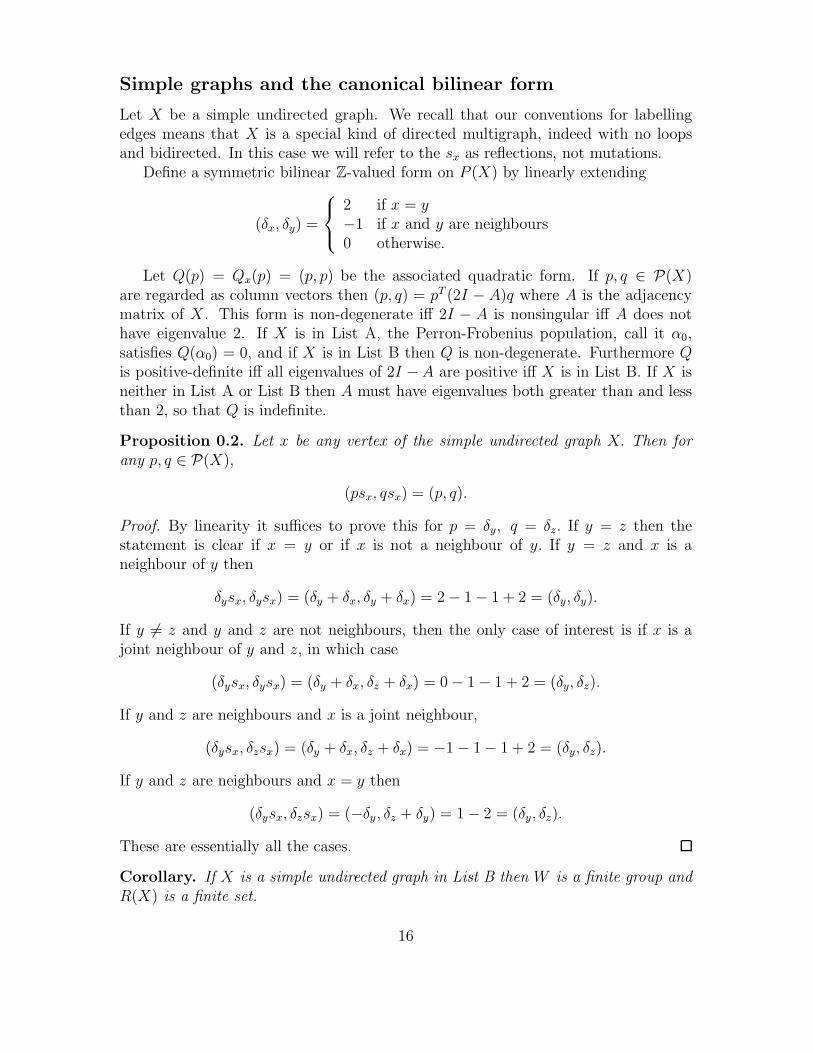
Simple graphs and the canonical bilinear form

Let X be a simple undirected graph. We recall that our conventions for labellingedges means that X is a special kind of directed multigraph, indeed with no loopsand bidirected. In this case we will refer to the sx as reflections, not mutations.

Define a symmetric bilinear Z-valued form on P (X) by linearly extending

(δx, δy) =

⎧⎨⎩

2 if x = y−1 if x and y are neighbours0 otherwise.

Let Q(p) = Qx(p) = (p, p) be the associated quadratic form. If p, q ∈ P(X)are regarded as column vectors then (p, q) = pT (2I − A)q where A is the adjacencymatrix of X. This form is non-degenerate iff 2I − A is nonsingular iff A does nothave eigenvalue 2. If X is in List A, the Perron-Frobenius population, call it α0,satisfies Q(α0) = 0, and if X is in List B then Q is non-degenerate. Furthermore Qis positive-definite iff all eigenvalues of 2I −A are positive iff X is in List B. If X isneither in List A or List B then A must have eigenvalues both greater than and lessthan 2, so that Q is indefinite.

Proposition 0.2. Let x be any vertex of the simple undirected graph X. Then forany p, q ∈ P(X),

(psx, qsx) = (p, q).

Proof. By linearity it suffices to prove this for p = δy, q = δz. If y = z then thestatement is clear if x = y or if x is not a neighbour of y. If y = z and x is aneighbour of y then

δysx, δysx) = (δy + δx, δy + δx) = 2 − 1 − 1 + 2 = (δy, δy).

If y �= z and y and z are not neighbours, then the only case of interest is if x is ajoint neighbour of y and z, in which case

(δysx, δysx) = (δy + δx, δz + δx) = 0 − 1 − 1 + 2 = (δy, δz).

If y and z are neighbours and x is a joint neighbour,

(δysx, δzsx) = (δy + δx, δz + δx) = −1 − 1 − 1 + 2 = (δy, δz).

If y and z are neighbours and x = y then

(δysx, δzsx) = (−δy, δz + δy) = 1 − 2 = (δy, δz).

These are essentially all the cases.

Corollary. If X is a simple undirected graph in List B then W is a finite group andR(X) is a finite set.

16

Proof. This follows from the discreteness of W , the fact that Q is positive definiteand that W preserves Q, and the fact that R(X) is at most a finite union of Worbits.

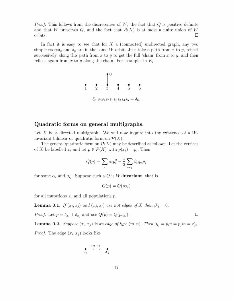
In fact it is easy to see that for X a (connected) undirected graph, any twosimple rootsδx and δy are in the same W orbit. Just take a path from x to y, reflectsuccessively along this path from x to y to get the full ‘chain’ from x to y, and thenreflect again from x to y along the chain. For example, in E7

1 2 3 4 5 6

0

δ0 s3s4s5s6s0s3s4s5 = δ6.

Quadratic forms on general multigraphs.

Let X be a directed multigraph. We will now inquire into the existence of a W -invariant bilinear or quadratic form on P(X).

The general quadratic form on P(X) may be described as follows. Let the verticesof X be labelled xi and let p ∈ P(X) with p(xi) = pi. Then

Q(p) =∑i

αip2i −

1

2

∑i�=j

βijpipj

for some αi and βij . Suppose such a Q is W -invariant, that is

Q(p) = Q(psx)

for all mutations sx and all populations p.

Lemma 0.1. If (xi, xj) and (xj , xi) are not edges of X then βij = 0.

Proof. Let p = δxi+ δxj

and use Q(p) = Q(psxi).

Lemma 0.2. Suppose (xi, xj) is an edge of type (m,n). Then βij = pin = pjm = βji.

Proof. The edge (xi, xj) looks like

xi xj

m n

17

Let p = piδxi+ pjδxj

. Then

Q(p) = αip2i + αjp

2j − βijpipj = Q(psxi

)

= Q(δxi(−pi + npj) + pjδxj

)

= αi(−pi + npj)2 + αjp

2j − βij(−pi + npj)pj

= αip2i + (αj + αin

2 − βijn)p2j − (2αin− βij)pipj

In order for this equality to hold for all pi and pj we need

αin2 − βijn = 0

and

βij = 2αin− βij ,

that is, we need βij = 2αin. Symmetrically we get βij = αjm.

A W -invariant Q is thus determined by the weights αi, which must necessarilysatisfy the equalities

αin = αjm

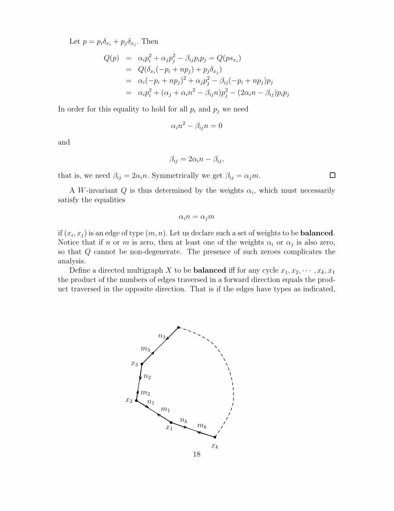
if (xi, xj) is an edge of type (m,n). Let us declare such a set of weights to be balanced.Notice that if n or m is zero, then at least one of the weights αi or αj is also zero,so that Q cannot be non-degenerate. The presence of such zeroes complicates theanalysis.

Define a directed multigraph X to be balanced iff for any cycle x1, x2, · · · , xk, x1

the product of the numbers of edges traversed in a forward direction equals the prod-uct traversed in the opposite direction. That is if the edges have types as indicated,

n3

m3

x3

n2

m2

m1

n1

x1

x2

xk

mk

nk

18

then m1m2 · · ·mk = n1n2 · · ·nk.Lemma 0.3. Let X be a bidirected multigraph with no loops. Then X has a balancedset of weights iff X is balanced.

Proof. If αi is a balanced set of weights on X then on the cycle x1, x2, · · · , xk, x1

pictured above we must have the equalities α1n1 = α2m1, α2n2 = α3m2, · · ·αknk =α1mk. Taking the product gives

α1α2 · · ·αk n1 · · ·nk = α1 · · ·αk m1 · · ·mk.

If one of the αi is zero they all are, which we don’t allow, so that n1 · · ·nk = m1 · · ·mk.Conversely given a balanced X we may assign a weight of say α1 = 1 to x1 and

then all other weights are determined by connectivity and the bidirected nature ofX. Consistency of choices is just equivalent to the above product equality around anycycle.

Note that the weight function is unique up to a constant.

Theorem 0.7. Let X be a balanced bidirected multigraph with no loops. Then P(X)has a W -invariant quadratic form, unique up to a constant.

Proof. Let X be a balanced bidirected multigraph with no loops, and let {αi} be abalanced set of weights on the vertices. For any i, j let us agree that the edge typeof (xi, xj) be (mij , nij) even if these are both zero.

Set

βij = αjmij = αinij = βji

which is well-defined by our assumption, and let

Q(p) =∑i

αip2i −

1

2

∑i�=j

βijpipj.

Fix a vertex xk. Applying sk to p changes pk to −pk+∑

� �=k nk�p� and leaves the otherpi unchanged.

Thus

Q(psk) =∑i�=k

αip2i + αk(−pk +

∑� �=k

nk�p�)2 − 1

2

∑i�=j

i�=k �=j

βijpipj

−1

2

∑j �=k

βkj(−pk +∑� �=k

nk�p�)pj

−1

2

∑i�=k

βikpi(−pk +∑� �=k

nk�p�).

19

In this expression, the coefficient of p2i , i �= k, is

αi + αkn2ki −

1

2βkinki − 1

2βiknki = αi + βkinki − βkinki

= αi.

The coefficient of p2k is αk. The coefficient of pipj for i �= k, j �= k, i �= j is

2αknkinkj − 1

2(βij + βji) − 1

2(βkjnki + βkinkj) − 1

2(βiknkj + βjknki)

= 2αknkinkj − βij − βkinkj − βkjnki

= −βij + 2αknkinkj − αknkinkj − αknkjnki

= −βij ,

which is also the coefficient of pipj in Q(p). Finally, the coefficient of pipk for i �= k is

−2αknki +1

2βki +

1

2βik = −2αknki + βki

= −αknki= −βki

which is also in agreement with Q(p). Thus Q(p) = Q(psk) and we are done.

Corollary. If X is a bidirected multigraph which is a tree, then P(X) has a W -invariant quadratic form, unique up to a constant.

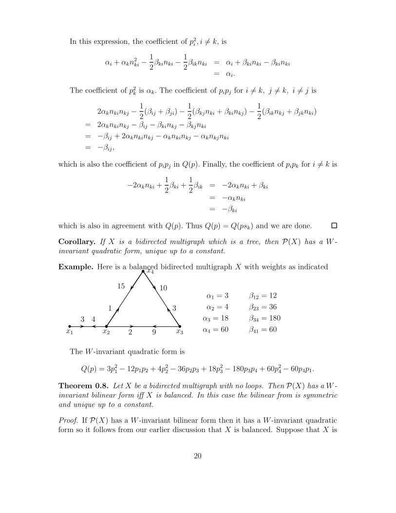
Example. Here is a balanced bidirected multigraph X with weights as indicated

x1 x2 x32 9

3 4

x4

15

1 3

10α1 = 3 β12 = 12

α2 = 4 β23 = 36

α3 = 18 β34 = 180

α4 = 60 β41 = 60

The W -invariant quadratic form is

Q(p) = 3p21 − 12p1p2 + 4p2

2 − 36p2p3 + 18p23 − 180p3p4 + 60p2

4 − 60p4p1.

Theorem 0.8. Let X be a bidirected multigraph with no loops. Then P(X) has a W -invariant bilinear form iff X is balanced. In this case the bilinear from is symmetricand unique up to a constant.

Proof. If P(X) has a W -invariant bilinear form then it has a W -invariant quadraticform so it follows from our earlier discussion that X is balanced. Suppose that X is

20

balanced with {αi} a balanced set of weights on the vertices and Q a W -invariantquadratic form. Define the symmetric bilinear form ( , ) by

(p, q) = (q, p) =1

4(Q(p+ q) −Q(p− q))

which is clearlyW -invariant. We need only show this is the only choice ofW -invariantbilinear form with associated quadratic form Q.

To this end, let 〈 , 〉 be an arbitrary such form. If (x, y) is an edge of type (m,n)then

〈δx, δy〉 = 〈δxsx, δysx〉= 〈−δx, δy + nδx〉= 〈δxsy, δysy〉= 〈δx +mδy,−δy〉

from which we deduce that

〈δx, δy〉 = −1

2nαx = −1

2mαy = 〈δy, δx〉.

Thus 〈 , 〉 is symmetric, which means it must coincide with ( , ).

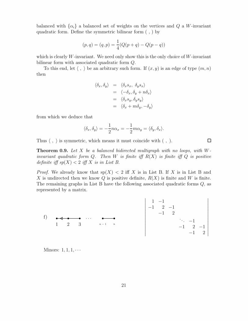
Theorem 0.9. Let X be a balanced bidirected multigraph with no loops, with W -invariant quadratic form Q. Then W is finite iff R(X) is finite iff Q is positivedefinite iff sp(X) < 2 iff X is in List B.

Proof. We already know that sp(X) < 2 iff X is in List B. If X is in List B andX is undirected then we know Q is positive definite, R(X) is finite and W is finite.The remaining graphs in List B have the following associated quadratic forms Q, asrepresented by a matrix.

f) . . .

n − 1 n1 2 3

∣∣∣∣∣∣∣∣∣∣∣∣∣

1 −1−1 2 −1

−1 2. . . −1−1 2 −1

−1 2

∣∣∣∣∣∣∣∣∣∣∣∣∣

Minors: 1, 1, 1, · · ·

21

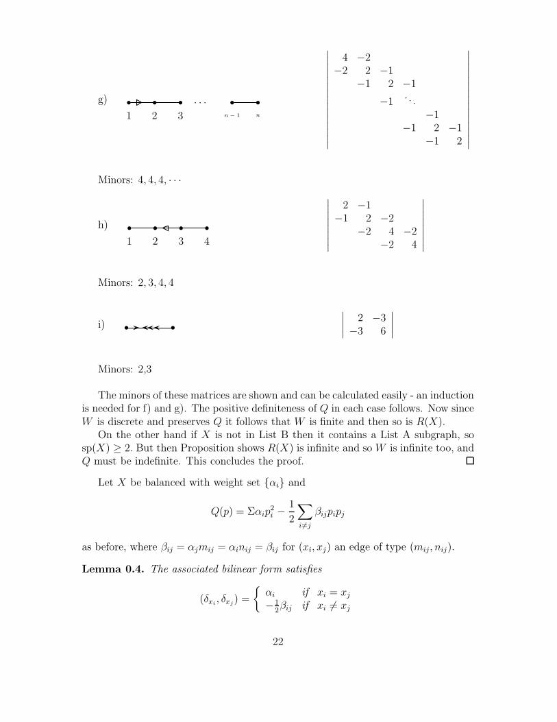
g) . . .

n − 1 n1 2 3

∣∣∣∣∣∣∣∣∣∣∣∣∣∣∣

4 −2−2 2 −1

−1 2 −1

−1. . .

−1−1 2 −1

−1 2

∣∣∣∣∣∣∣∣∣∣∣∣∣∣∣

Minors: 4, 4, 4, · · ·

h)

1 2 3 4

∣∣∣∣∣∣∣∣2 −1

−1 2 −2−2 4 −2

−2 4

∣∣∣∣∣∣∣∣

Minors: 2, 3, 4, 4

i)

∣∣∣∣ 2 −3−3 6

∣∣∣∣

Minors: 2,3

The minors of these matrices are shown and can be calculated easily - an inductionis needed for f) and g). The positive definiteness of Q in each case follows. Now sinceW is discrete and preserves Q it follows that W is finite and then so is R(X).

On the other hand if X is not in List B then it contains a List A subgraph, sosp(X) ≥ 2. But then Proposition shows R(X) is infinite and so W is infinite too, andQ must be indefinite. This concludes the proof.

Let X be balanced with weight set {αi} and

Q(p) = Σαip2i −

1

2

∑i�=j

βijpipj

as before, where βij = αjmij = αinij = βij for (xi, xj) an edge of type (mij, nij).

Lemma 0.4. The associated bilinear form satisfies

(δxi, δxj

) =

{αi if xi = xj−1

2βij if xi �= xj

22

Proof. i) If xi = xj then

(δxi, δxi

) =1

4(Q(δxi

+ δxi) −Q(δxi

− δxi)) = αi

ii) while if xi �= xj then

(δxi, δxj

) =1

4(Q(δxi

+ δxj) −Q(δxi

− δxj))

= −1

2βij.

Remark. In the list A and B graphs, the βij are even if the αi are chosen to beeven. Clearly we can choose the αi so that all the αi and βij are integers, which wehenceforth assume.

Explicit Posets of Positive Roots

Let X be a bi-directed multigraph with no loops, and R+(X) the set of positive rootsof X. Declare p ≤ q iff p(x) ≤ q(x) for all vertices x, and p ≤ q iff p ≤ q and qis obtained from q by a series of mutations that increase populations. Let R++(X)denote the set R+(X) with the partial order ≤; with the partial order ≤ we refer toR+(X).

We now list explicitly all the posets so obtained, with the infinite series beingindicated by a representative sampling - the pattern is in all cases obvious [hope-fully]. It is practical to depict the reverse Hasse diagrams of posets. Another usefulconvention is to indicate the difference between adjacent roots, necessarily a multipleof a simple root, or vertex, by a multiple edge.

23

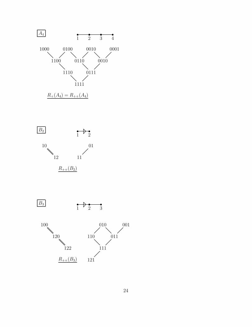
A4

1 2 3 4

1000 0100 0010 0001

1100 0110 0010

1110 0111

1111

R+(A4) = R++(A4)

B2

1 2

10 01

12 11

R++(B2)

B3

1 2 3

100

120

122

010 001

110 011

111

121R++(B3)

24

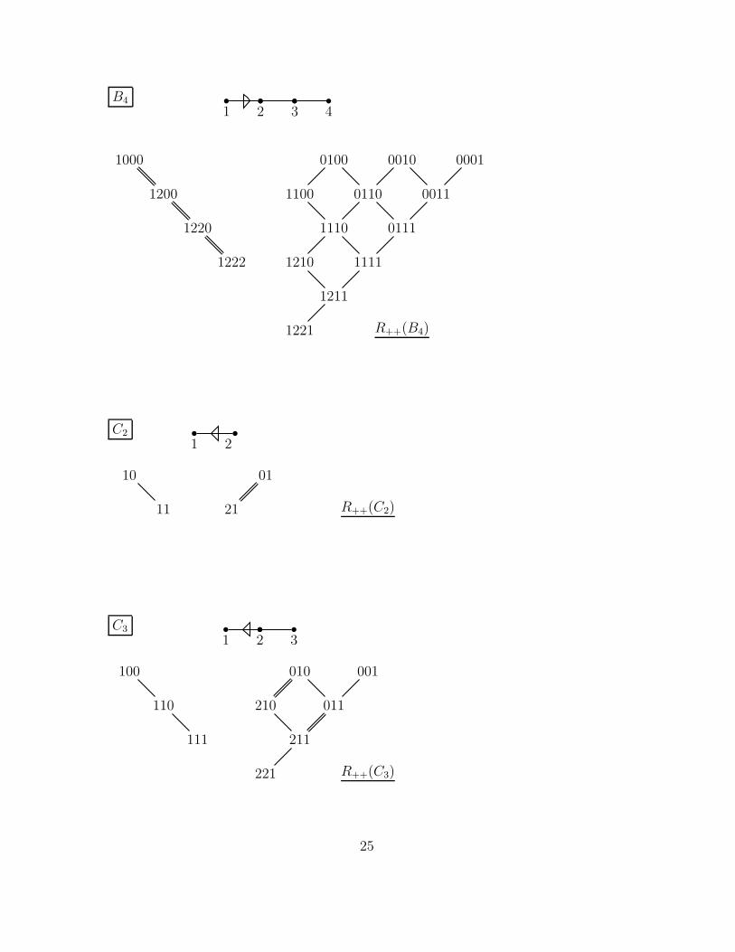
B4

1 2 3 4

1000

1200

1220

1222

0100 0010 0001

1100 0110 0011

1110 0111

1210 1111

1211

1221 R++(B4)

C2

1 2

10 01

11 21 R++(C2)

C3

1 2 3

100

110

111

010 001

210 011

211

221 R++(C3)

25

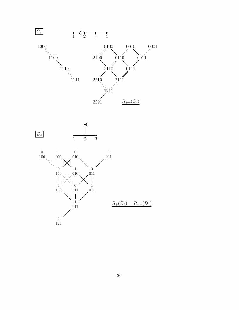
C4

1 2 3 4

1000

1100

1110

1111

0100 0010 0001

2100 0110 0011

2110 0111

2210 2111

1211

2221 R++(C4)

D4

1 2 3

0

0100

1000

0010

0001

0110

1010

0011

1110

0111

1011

1111

1121

R+(D4) = R++(D4)

26

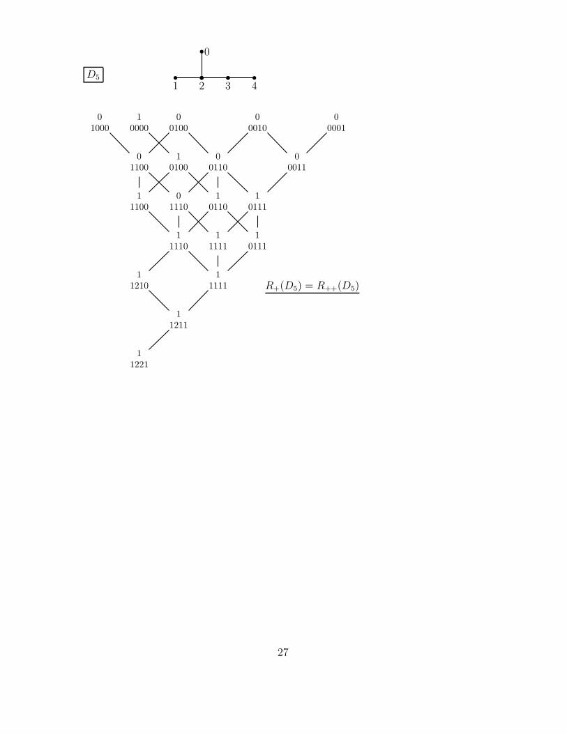
D5

1 2 3 4

0

01000

10000

00100

00010

00001

01100

10100

00110

00011

11100

01110

10110

10111

11110

11111

10111

11210

11111

11211

11221

R+(D5) = R++(D5)

27

E6

1 2 3 4 5

0

010000

000010

100000

000100

000010

000001

011000

001100

100100

000110

000011

011100

101100

001110

100110

000111

111100

011110

101110

101111

100111

111110

011111

101210

101111

111210

111111

111110

112210

111211

101221

112211

111221

112221

112321

212321

R+(E6) = R++(E6)

28

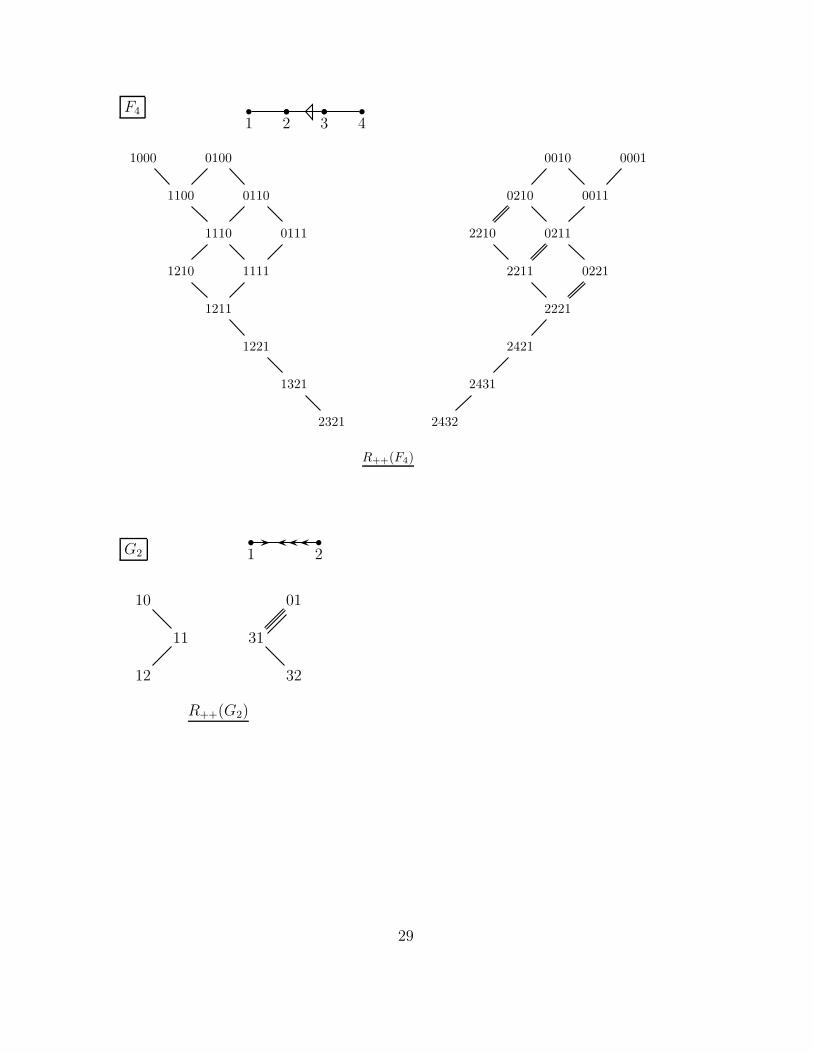
F4

1 2 3 4

1000 0100 0010 0001

1100 0110 0210 0011

1110 0111 2210 0211

1210 1111 2211 0221

1211 2221

1221 2421

1321 2431

2321 2432

R++(F4)

G2 1 2

10 01

11 31

12 32

R++(G2)

29

The Dual Mutation Game

Venus is populated by Venetians and anti-Venetians, who, like the inhabitants ofMars, live in a network of cities connected by one way roads. The only differenceis what happens when a city on Venus mutates. In this case, the city clones itselfsufficiently to send an army down every road leading away from the city while itsoriginal population all change their type.

Here is an example of three cities A,B,C with populations 12,5 and 1 respectively.

• •

•

12A

B

C1

5

A dual mutation at A results in populations of −12, 17, 13 respectively. A subsequentdual mutation at B results in populations of 22,−17 and 47 respectively. For reasonsthat will become clear shortly, we prefer to think of dual mutations as acting on anidentical but separate space of dual populations where X is the underlying directedmultigraph of cities and roads on Venus. We will denote the singleton dual populationat x by εx, and refer to it as the fundamental weight at the vertex x. Any dualpopulation obtainable from a fundamental weight by a series of dual mutations willbe called a weight and the set of all weights of X will be denoted Q(X ).

More precisely for a vertex x and a dual population q, we define the dual muta-tion/reflection rx at x by

(qrx)(y) =

{ −q(y) if y = xq(y) + A(x, y)q(x) if y �= x

Theorem 0.10. If x and y are vertices of X then

i) r2x = identity

ii) rxry = ryrx if x and y are not neighbours

iii) rxry has finite order greater than 2 iff the edge type of (x, y) is a) (1, 1) b)(1, 2) or (2, 1) or c) (1, 3) or (3, 1) in which case rxry has order a) 3 b) 4 orc) 6 respectively.

30

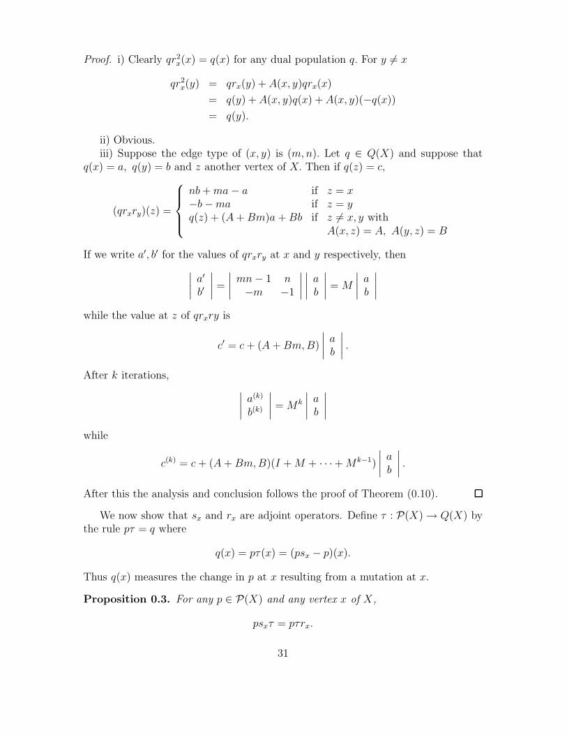
Proof. i) Clearly qr2x(x) = q(x) for any dual population q. For y �= x

qr2x(y) = qrx(y) + A(x, y)qrx(x)

= q(y) + A(x, y)q(x) + A(x, y)(−q(x))= q(y).

ii) Obvious.iii) Suppose the edge type of (x, y) is (m,n). Let q ∈ Q(X) and suppose that

q(x) = a, q(y) = b and z another vertex of X. Then if q(z) = c,

(qrxry)(z) =

⎧⎪⎪⎨⎪⎪⎩

nb+ma− a if z = x−b−ma if z = yq(z) + (A+Bm)a +Bb if z �= x, y with

A(x, z) = A, A(y, z) = B

If we write a′, b′ for the values of qrxry at x and y respectively, then∣∣∣∣ a′b′∣∣∣∣ =

∣∣∣∣ mn− 1 n−m −1

∣∣∣∣∣∣∣∣ ab

∣∣∣∣ = M

∣∣∣∣ ab∣∣∣∣

while the value at z of qrxry is

c′ = c+ (A +Bm,B)

∣∣∣∣ ab∣∣∣∣ .

After k iterations, ∣∣∣∣ a(k)

b(k)

∣∣∣∣ = Mk

∣∣∣∣ ab∣∣∣∣

while

c(k) = c + (A+Bm,B)(I +M + · · ·+Mk−1)

∣∣∣∣ ab∣∣∣∣ .

After this the analysis and conclusion follows the proof of Theorem (0.10).

We now show that sx and rx are adjoint operators. Define τ : P(X) → Q(X) bythe rule pτ = q where

q(x) = pτ(x) = (psx − p)(x).

Thus q(x) measures the change in p at x resulting from a mutation at x.

Proposition 0.3. For any p ∈ P(X) and any vertex x of X,

psxτ = pτrx.

31

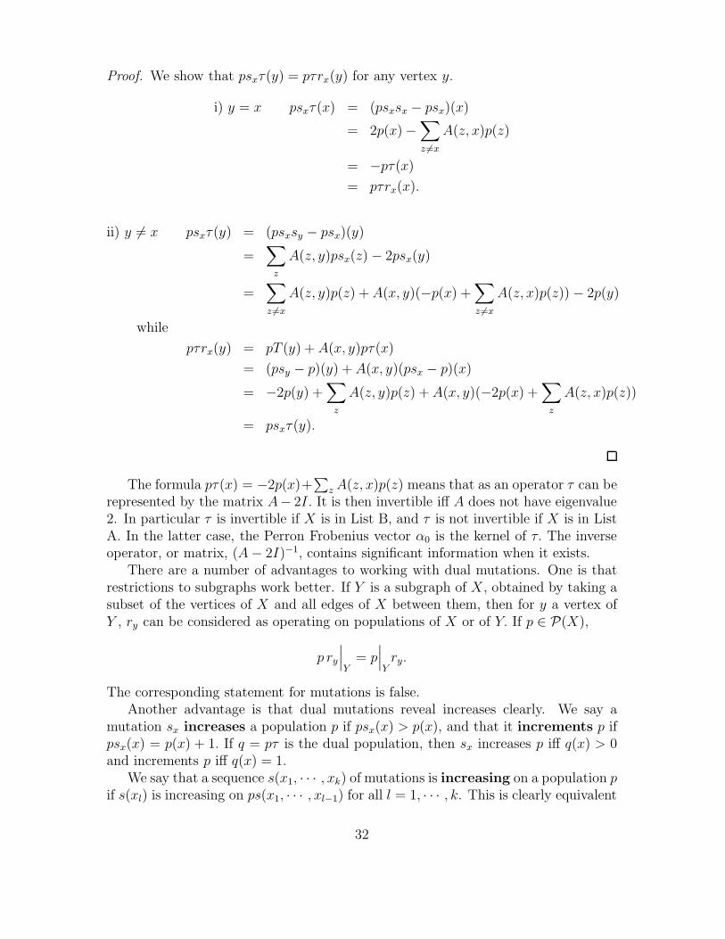
Proof. We show that psxτ(y) = pτrx(y) for any vertex y.

i) y = x psxτ(x) = (psxsx − psx)(x)

= 2p(x) −∑z �=x

A(z, x)p(z)

= −pτ(x)= pτrx(x).

ii) y �= x psxτ(y) = (psxsy − psx)(y)

=∑z

A(z, y)psx(z) − 2psx(y)

=∑z �=x

A(z, y)p(z) + A(x, y)(−p(x) +∑z �=x

A(z, x)p(z)) − 2p(y)

while

pτrx(y) = pT (y) + A(x, y)pτ(x)

= (psy − p)(y) + A(x, y)(psx − p)(x)

= −2p(y) +∑z

A(z, y)p(z) + A(x, y)(−2p(x) +∑z

A(z, x)p(z))

= psxτ(y).

The formula pτ(x) = −2p(x)+∑

z A(z, x)p(z) means that as an operator τ can berepresented by the matrix A− 2I. It is then invertible iff A does not have eigenvalue2. In particular τ is invertible if X is in List B, and τ is not invertible if X is in ListA. In the latter case, the Perron Frobenius vector α0 is the kernel of τ. The inverseoperator, or matrix, (A− 2I)−1, contains significant information when it exists.

There are a number of advantages to working with dual mutations. One is thatrestrictions to subgraphs work better. If Y is a subgraph of X, obtained by taking asubset of the vertices of X and all edges of X between them, then for y a vertex ofY , ry can be considered as operating on populations of X or of Y. If p ∈ P(X),

p ry

∣∣∣Y

= p∣∣∣Yry.

The corresponding statement for mutations is false.Another advantage is that dual mutations reveal increases clearly. We say a

mutation sx increases a population p if psx(x) > p(x), and that it increments p ifpsx(x) = p(x) + 1. If q = pτ is the dual population, then sx increases p iff q(x) > 0and increments p iff q(x) = 1.

We say that a sequence s(x1, · · · , xk) of mutations is increasing on a population pif s(xl) is increasing on ps(x1, · · · , xl−1) for all l = 1, · · · , k. This is clearly equivalent

32

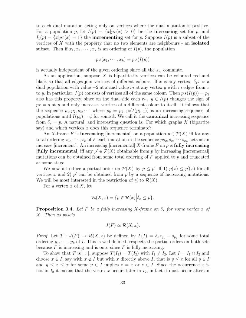
to each dual mutation acting only on vertices where the dual mutation is positive.For a population p, let I(p) = {x|pτ(x) > 0} be the increasing set for p, andI1(p) = {x|pτ(x) = 1} the incrementing set for p. Suppose I(p) is a subset of thevertices of X with the property that no two elements are neighbours - an isolatedsubset. Then if x1, x2, · · · , xk is an ordering of I(p), the population

p s(x1, · · · , xk) = p s(I(p))

is actually independent of the given ordering since all the sxicommute.

As an application, suppose X is bipartite-its vertices can be coloured red andblack so that all edges join vertices of different colours. If x is any vertex, δxτ is adual population with value −2 at x and value m at any vertex y with m edges from xto y. In particular, I(p) consists of vertices all of the same colour. Then p s(I(p)) = p2

also has this property, since on the dual side each rY , y ∈ I(p) changes the sign ofpτ = q at y and only increases vertices of a different colour to itself. It follows thatthe sequence p1, p2, p3, · · · where pk = pk−1s(I(pk−1)) is an increasing sequence ofpopulations until I(pk) = φ for some k. We call it the canonical increasing sequencefrom δx = p. A natural, and interesting question is: For which graphs X (bipartitesay) and which vertices x does this sequence terminate?

An X-frame F is increasing [incremental] on a population p ∈ P(X) iff for anytotal ordering x1, · · · , xk of F each mutation in the sequence psx1sx2 · · · sxk

acts as anincrease [increment]. An increasing [incremental] X-frame F on p is fully increasing[fully incremental] iff any p′ ∈ P(X) obtainable from p by increasing [incremental]mutations can be obtained from some total ordering of F applied to p and truncatedat some stage.

We now introduce a partial order on P(X) by p ≤ p′ iff 1) p(x) ≤ p′(x) for allvertices x and 2) p′ can be obtained from p by a sequence of increasing mutations.We will be most interested in the restriction of ≤ to R(X).

For a vertex x of X, let

R(X, x) = {p ∈ R(x)∣∣∣δx ≤ p}.

Proposition 0.4. Let F be a fully increasing X-frame on δx for some vertex x ofX. Then as posets

J(F ) � R(X, x).

Proof. Let T : J(F ) → R(X, x) be defined by T (I) = δxsy1 − sykfor some total

ordering y1, · · · , yk of I. This is well defined, respects the partial orders on both setsbecause F is increasing and is onto since F is fully increasing.

To show that T is | : |, suppose T (I1) = T (I2) with I1 �= I2. Let I = I1 ∩ I2 andchoose x ∈ I, say with x �∈ I but with x directly above I, that is y ≤ x for all y ∈ Iand y ≤ z ≤ x for some y ∈ I implies z = x or z ∈ I. Since the occurrence x isnot in I2 it means that the vertex x occurs later in I2, in fact it must occur after an

33

occurrence of some neighbouring vertex say z. That means when x does occur in I2,the correspondence mutation increases x more than does the occurrence of x in I,directly after I. It follows that δws(I)sx.

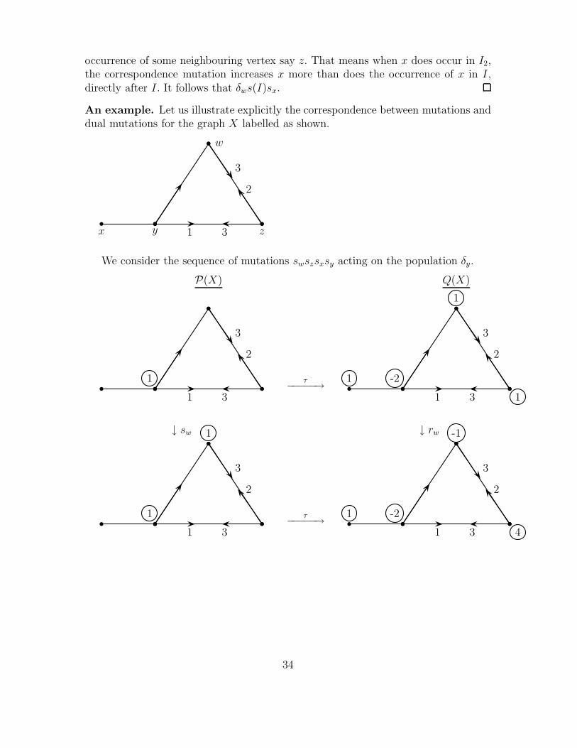
An example. Let us illustrate explicitly the correspondence between mutations anddual mutations for the graph X labelled as shown.

x y z1 3

w

2

3

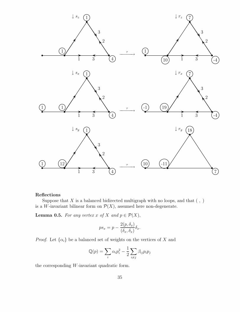
We consider the sequence of mutations swszsxsy acting on the population δy.

1 3

2

3

P(X)

1 τ−−−−−→1 3

2

3

1

1 -2

1

Q(X)

1 3

2

3

1

1

↓ sw

τ−−−−−→1 3

2

3

-1

1 -2

4

↓ rw

34

1 3

2

3

1

1

↓ sz

4

τ−−−−−→1 3

2

3

7

1

10 -4

↓ rz

1 3

2

3

1

11

↓ sx

4

τ−−−−−→1 3

2

3

7

-1 19

-4

↓ rx

1 3

2

3

1

121

↓ sy

4

τ−−−−−→

18

10 -11

7

↓ ry

ReflectionsSuppose that X is a balanced bidirected multigraph with no loops, and that ( , )

is a W -invariant bilinear form on P(X), assumed here non-degenerate.

Lemma 0.5. For any vertex x of X and p ∈ P(X),

psx = p− 2(p, δx)

(δx, δx)δx.

Proof. Let {αi} be a balanced set of weights on the vertices of X and

Q(p) =∑i

αip2i −

1

2

∑i�=j

βijpipj

the corresponding W -invariant quadratic form.

35

Then (δx, δx) = αx and

(p, δx) = p(x)αx − 1

2

∑y �=x

βyxp(y).

But βyx = αxmyx where myx = A(y, x). Thus

(p, δx) = αx(p(x) =1

2

∑y �=x

myxp(y))

and

p− 2(p, δx)

(δx, δx)δx = p− (2p(x)δx −

∑y �=x

myxp(y)δx)

= psx.

Note that this identifies sx as a legitimate reflection with respect to ( , ) on P(X).Let P�(X) denote the space of Q-valued functions on the vertices of X. The

previous Lemma motivates us to define, for any q ∈ P(X), the operator

psq = p− 2(p, q)

(q, q)q

acting on P�(X), which we call the reflection at p.

Proposition 0.5. Let p, q ∈ P(X). Then s−1q = sq and

sqsp = s−1p sqsp = spsqsp.

Proof. For any r ∈ P�(X),

r sqsp = r − 2(r, qsp)

(qsp, qsp)qsp.

Here (qsp, qsp) refers to the Q-linear extension of ( , ) to P�(X). One checks easilythat (qsp, q, sp) = (q, q). In fact for any q, q′ ∈ P(X)

(qsp, q′sp) = (q − 2

(q, p)

(p, p)p, q′ − 2

(q′, p)(p, p)

p)

= (q, q′) − 2(q, p)(p, q′)

(p, p)− 2

(q′, p)(p, q)(p, p)

+ 4(q, p)(q′, p)

(p, p)

= (q, q′).

36

Thus

rsqsp = r − 2(rs−1

p , q)

(q, q)qsp.

= (rs−1p − 2

(rs−1p , q)

(q, q)q)sp

= rs−1p sqsp.

Finally,

ps2q = psq − 2

(psq, q)

(q, q)q

= p− 2(p, q)

(q, q)q − 2

(p, q)

(q, q)q + 4

(p, q)

(q, q)

(q, q)

(q, q)q

= p

so s−1q = sq.

Corollary. For p ∈ R(X), P(X)sp = P(X).

Proof. Clearly sx takes P(X) to P(X) for any vertex x. Since any root p ∈ R(X)is obtained from a simple root by reflections, we may write p = δxsy, sy1sy2 · · · syk

forsome vertices x, y1, · · · , yk. But then

sp = syk· · · sy1sxsy1 · · · syk

so sp takes P(X) to P(X).

Let T = {sp∣∣∣p ∈ R(X)} ⊆ W. We call T the set of reflections in W . The above

shows that T consists exactly of the conjugates of S = {sx∣∣∣x a vertex of X} in W.

Proposition 0.6. The map p �→ sp establishes a bijection between R(X) and T.

Proof. If sp = sq then

psp = −p = psq = p− 2(p, q)

(q, q)q

so that 2p = 2(p, q)

(q, q)q. Thus p and q are multiples, i.e. (q, q)p = (p, q)q. But by

symmetry, (p, p)q = (q, p)p. Thus (q, q)(p, p) = (p, q)2. Suppose p is derived from thesimple root δx, and q is derived from the simple root δy. But then δxw is a multipleof δy for some w and conversely δyv is a multiple of δx for some v in W . But sinceW acts invertibly on P(X), these multiples must be 1, and p = q.

37

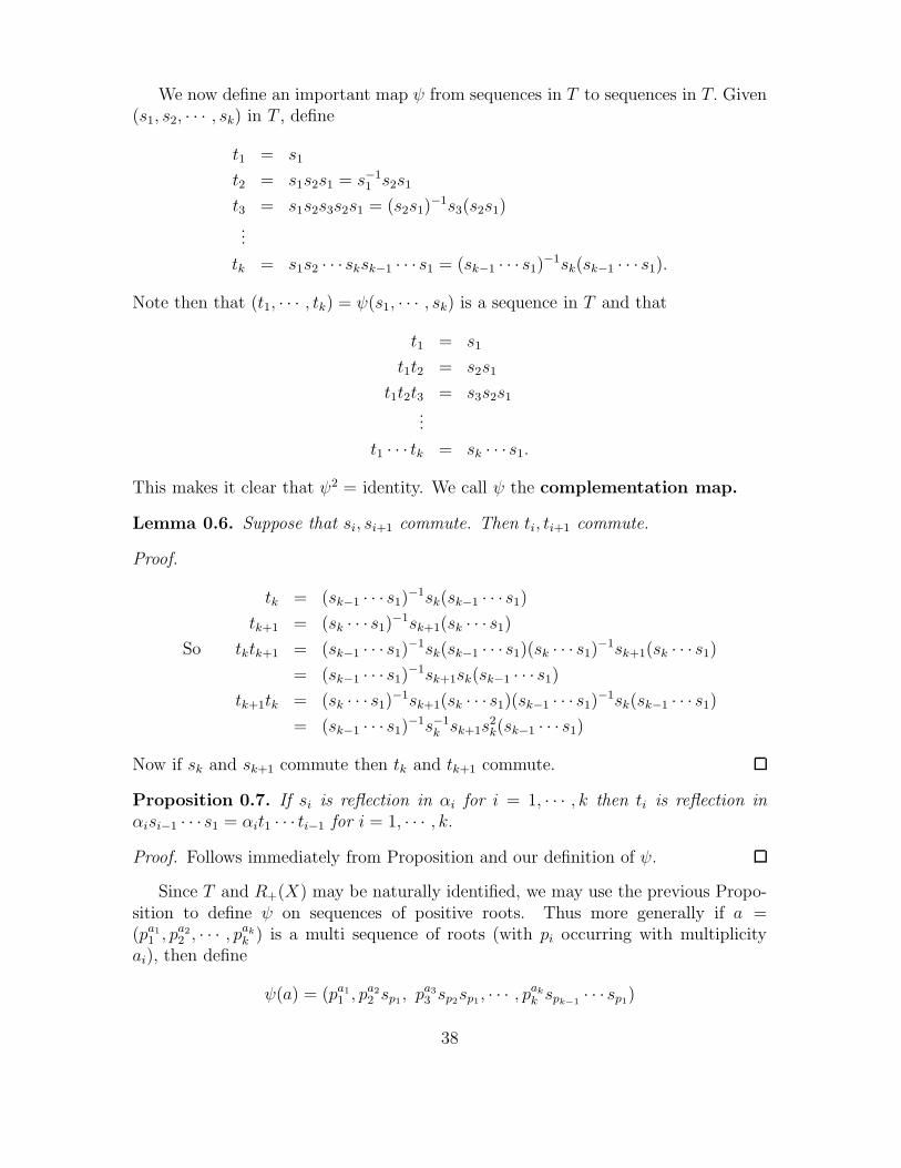
We now define an important map ψ from sequences in T to sequences in T. Given(s1, s2, · · · , sk) in T , define

t1 = s1

t2 = s1s2s1 = s−11 s2s1

t3 = s1s2s3s2s1 = (s2s1)−1s3(s2s1)

...

tk = s1s2 · · · sksk−1 · · · s1 = (sk−1 · · · s1)−1sk(sk−1 · · · s1).

Note then that (t1, · · · , tk) = ψ(s1, · · · , sk) is a sequence in T and that

t1 = s1

t1t2 = s2s1

t1t2t3 = s3s2s1

...

t1 · · · tk = sk · · · s1.

This makes it clear that ψ2 = identity. We call ψ the complementation map.

Lemma 0.6. Suppose that si, si+1 commute. Then ti, ti+1 commute.

Proof.

tk = (sk−1 · · · s1)−1sk(sk−1 · · · s1)

tk+1 = (sk · · · s1)−1sk+1(sk · · · s1)

So tktk+1 = (sk−1 · · · s1)−1sk(sk−1 · · · s1)(sk · · · s1)

−1sk+1(sk · · · s1)

= (sk−1 · · · s1)−1sk+1sk(sk−1 · · · s1)

tk+1tk = (sk · · · s1)−1sk+1(sk · · · s1)(sk−1 · · · s1)

−1sk(sk−1 · · · s1)

= (sk−1 · · · s1)−1s−1

k sk+1s2k(sk−1 · · · s1)

Now if sk and sk+1 commute then tk and tk+1 commute.

Proposition 0.7. If si is reflection in αi for i = 1, · · · , k then ti is reflection inαisi−1 · · · s1 = αit1 · · · ti−1 for i = 1, · · · , k.Proof. Follows immediately from Proposition and our definition of ψ.

Since T and R+(X) may be naturally identified, we may use the previous Propo-sition to define ψ on sequences of positive roots. Thus more generally if a =(pa11 , p

a22 , · · · , pak

k ) is a multi sequence of roots (with pi occurring with multiplicityai), then define

ψ(a) = (pa11 , pa22 sp1, p

a33 sp2sp1, · · · , pak

k spk−1· · · sp1)

38

where by convention paii spj

= (pispj)ai . Note that this is just linearity of the spj

;afterall pai

i is just a notational shorthand for aipi.We should also warn the reader that even though all the pi may be positive roots,

there is no guarantee that each element of ψ(a) is a positive root - in general it willbe only a multiple of a root.

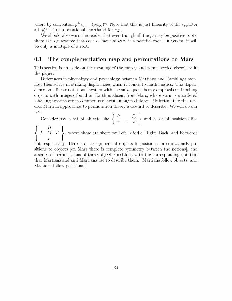
0.1 The complementation map and permutations on Mars

This section is an aside on the meaning of the map ψ and is not needed elsewhere inthe paper.

Differences in physiology and psychology between Martians and Earthlings man-ifest themselves in striking disparencies when it comes to mathematics. The depen-dence on a linear notational system with the subsequent heavy emphasis on labellingobjects with integers found on Earth is absent from Mars, where various unorderedlabelling systems are in common use, even amongst children. Unfortunately this ren-ders Martian approaches to permutation theory awkward to describe. We will do ourbest.

Consider say a set of objects like

{ � ©+ � ×

}and a set of positions like⎧⎨

⎩B

L M RF

⎫⎬⎭ , where these are short for Left, Middle, Right, Back, and Forwards

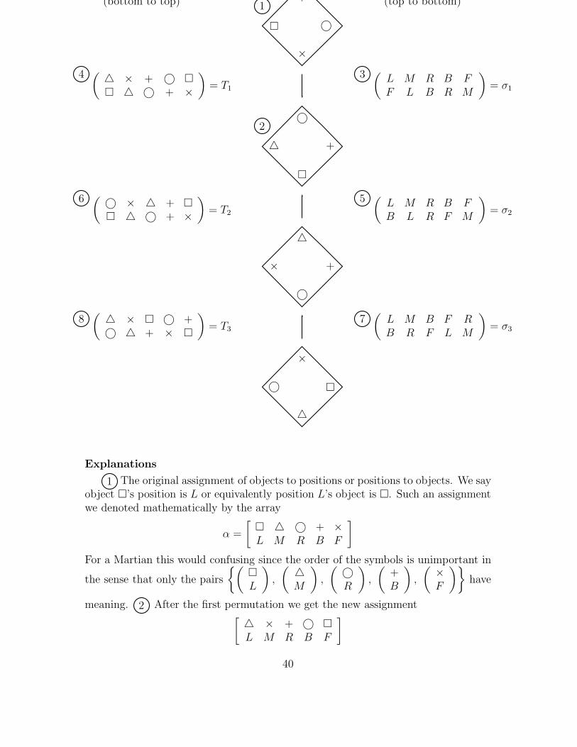
not respectively. Here is an assignment of objects to positions, or equivalently po-sitions to objects [on Mars there is complete symmetry between the notions], anda series of permutations of these objects/positions with the corresponding notationthat Martians and anti Martians use to describe them. [Martians follow objects; antiMartians follow positions.]

39

(bottom to top) (top to bottom)

4 ( � × + © �� � © + ×

)= T1

3 (L M R B FF L B R M

)= σ1

1+

×

� ©

6 ( © × � + �� � © + ×

)= T2

2©

�

� +

5 (L M R B FB L R F M

)= σ2

�

©

× +

8( � × � © +

© � + × �

)= T3

×

�

© �

7(L M B F RB R F L M

)= σ3

Explanations

1 The original assignment of objects to positions or positions to objects. We sayobject �’s position is L or equivalently position L’s object is �. Such an assignmentwe denoted mathematically by the array

α =

[� � © + ×L M R B F

]

For a Martian this would confusing since the order of the symbols is unimportant in

the sense that only the pairs

{(�L

),

( �M

),

( ©R

),

(+B

),

( ×F

)}have

meaning. 2 After the first permutation we get the new assignment[ � × + © �L M R B F

]

40

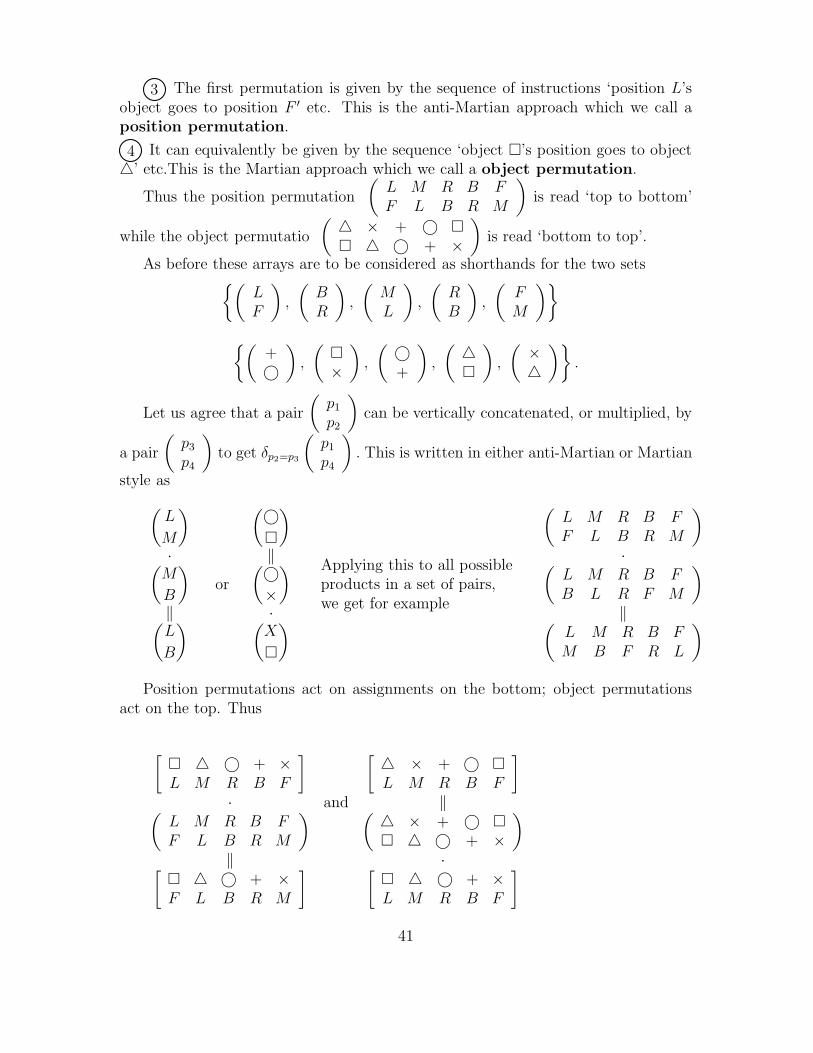
3 The first permutation is given by the sequence of instructions ‘position L’sobject goes to position F ′ etc. This is the anti-Martian approach which we call aposition permutation.

4 It can equivalently be given by the sequence ‘object �’s position goes to object�’ etc.This is the Martian approach which we call a object permutation.

Thus the position permutation

(L M R B FF L B R M

)is read ‘top to bottom’

while the object permutatio

( � × + © �� � © + ×

)is read ‘bottom to top’.

As before these arrays are to be considered as shorthands for the two sets{(LF

),

(BR

),

(ML

),

(RB

),

(FM

)}

{(+©

),

(�×

),

( ©+

),

( ��

),

( �

)}.

Let us agree that a pair

(p1

p2

)can be vertically concatenated, or multiplied, by

a pair

(p3

p4

)to get δp2=p3

(p1

p4

). This is written in either anti-Martian or Martian

style as

(L

M

)·(M

B

)‖(L

B

)or

(©�

)‖(©×

)·(X

�

)

Applying this to all possibleproducts in a set of pairs,we get for example

(L M R B FF L B R M

)·(

L M R B FB L R F M

)‖(

L M R B FM B F R L

)

Position permutations act on assignments on the bottom; object permutationsact on the top. Thus

[� � © + ×L M R B F

] [ � × + © �L M R B F

]· and ‖(

L M R B FF L B R M

) ( � × + © �� � © + ×

)‖ ·[

� � © + ×F L B R M

] [� � © + ×L M R B F

]

41

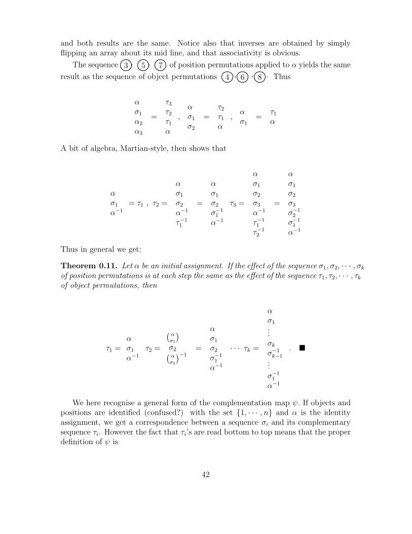
and both results are the same. Notice also that inverses are obtained by simplyflipping an array about its mid line, and that associativity is obvious.

The sequence 3 , 5 , 7 of position permutations applied to α yields the same

result as the sequence of object permutations 4 , 6 , 8 . Thus

ασ1

α2

α3

=

τ3τ2τ1α

,ασ1

σ2

=τ2τ1α

,ασ1

=τ1α

A bit of algebra, Martian-style, then shows that

ασ1

α−1

= τ1 , τ2 =

ασ1

σ2

α−1

τ−11

=

ασ1

σ2

σ−11

α−1

τ3 =

ασ1

σ2

σ3

α−1

τ−11

τ−12

=

ασ1

σ2

σ3

σ−12

σ−11

α−1

Thus in general we get:

Theorem 0.11. Let α be an initial assignment. If the effect of the sequence σ1, σ2, · · · , σkof position permutations is at each step the same as the effect of the sequence τ1, τ2, · · · , τkof object permutations, then

τ1 =ασ1

α−1

τ2 =

(ασ1

)σ2(ασ1

)−1=

ασ1

σ2

σ−11

α−1

· · · τk =

ασ1...σkσ−1k−1

...σ−1

1

α−1

. �

We here recognise a general form of the complementation map ψ. If objects andpositions are identified (confused?) with the set {1, · · · , n} and α is the identityassignment, we get a correspondence between a sequence σi and its complementarysequence τi. However the fact that τi’s are read bottom to top means that the properdefinition of ψ is

42

τ−11 = σ1

(τ1τ2)−1 = σ1σ2

(τ1τ2τ3)−1 = σ1σ2σ3

...

or

τ1 = σ−11

τ2 = σ1σ−12 σ−1

1

τ3 = σ1σ2σ−13 (σ1σ2)

−1

...

This happens to coincide with our earlier definition for reflections where each s2i = 1.

Posets, Lattices, and Generalisations

The mutation game associates to a multigraph X an interesting family of partiallyordered sets. In this section we review some necessary preliminaries, establish no-tation and discuss generalisations arising from the emphasis on multi-sets which weadopt.

Let (P,≤) be a partially ordered set, by which we mean that ≤ satisfies i)x ≤ x ii) x ≤ y and y ≤ x implies x = y iii) x ≤ y and y ≤ z implies x ≤ z. We sayy covers x iff x < y and x ≤ z < y implies z = x, and represent P by a reverseHasse diagram with elements of P as vertices and a downward line from x to y iffy covers x.

An ideal of P is a subset I such that y ∈ I, x ≤ y imply x ∈ I. A filter of Pis a subset J such that y ∈ J, y ≤ x imply x ∈ J. The set L(P ) of all ideals of P isitself a poset under inclusion.

A lattice is a poset P in which x∨y, the supremum or join of x and y, and x∧y,the infimum, or meet of x and y, are defined for all x, y. A lattice is distributiveiff for all x, y, z

x ∧ (y ∨ z) = (x ∧ y) ∨ (x ∧ z)

and modular iff for all x, y, z

x ≥ z ⇒ x ∧ (y ∨ z) = (x ∧ y) ∨ z.

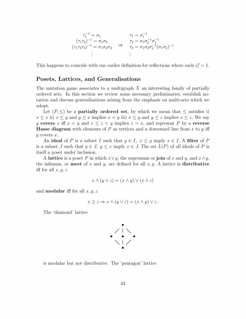
The ‘diamond’ lattice

•

• • •

•

is modular but not distributive. The ‘pentagon’ lattice

43

•

•

••

•

•

is neither modular nor distributive. [In fact any distributive lattice is modular].The standard example of a distributive lattice is a lattice of subsets of some set

under inclusion. The converse is included in this important result.

Theorem 0.12. Let L be a lattice. Then L is distributive iff one of the followingequivalent conditions hold.

i) L � L(P ) for some poset P ;

ii) L does not contain the diamond or pentagon lattices as sub-lattices.

In case L is distributive, the poset P may be identified in a natural way as theset of join-irreducible of L; those x ∈ L such that x �= 0 (in case L has a minimalelement 0, which ours do) and such that x = a∨ b implies x = a or x = b. Denote theset of join-irreducibles of L by J(L). In our situation join-irreducibles can be easilyidentified by the fact that they cover only one element. Thus L � L(JI(L)).

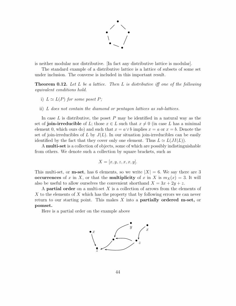
A multi-set is a collection of objects, some of which are possibly indistinguishablefrom others. We denote such a collection by square brackets, such as

X = [x, y, z, x, x, y].

This multi-set, or m-set, has 6 elements, so we write |X| = 6. We say there are 3occurrences of x in X, or that the multiplicity of x in X is mX(x) = 3. It willalso be useful to allow ourselves the convenient shorthand X = 3x+ 2y + z.

A partial order on a multi-set X is a collection of arrows from the elements ofX to the elements of X which has the property that by following errors we can neverreturn to our starting point. This makes X into a partially ordered m-set, orpomset.

Here is a partial order on the example above

•

•

x

z

• •

•x

z

•y

44

An arrow from y to x means x < y. The associated reverse Hasse diagram for thisexample is

x

y z

x x

z

We allow also the possibility of more than one arrow from y to x; this makes apomset just a special type of multi-graph. If furthermore several occurrences of anelement x are treated uniformly by a partial order, we will sometimes only indicatethe element with its multiplicity in a reverse Hasse diagram, expressed as an exponentor by circling. Hopefully the following makes this clear.

x y

z z

u w v

⇔ ⇔

x y

z2

u w v

x y

z

u w v

We adopt the convention that for small values of k, zk+1 is represented by zsurrounded by k circles.

Mutation Frames

Let X be a bidirected multigraph with no loops. We will be associating posets, calledframes, to sequences of vertices or mutations of X.

Given a sequence u = (x1, · · · , xk) of vertices of X, we refer to the xi as theoccurrences in the sequence, so that there are exactly k occurrences even if thexi’s repeat. Define two sequences u = (x1, x2, · · · , xk), u′ = (x′1, x

′2, · · · , x′k) to be

equivalent if one is obtained from the other by a finite number of switches of adjacentelements in the sequence whose corresponding vertices are not neighbours in X. Suchswitches we will call free switches.

Example.

45

1 2 3 4 5

0

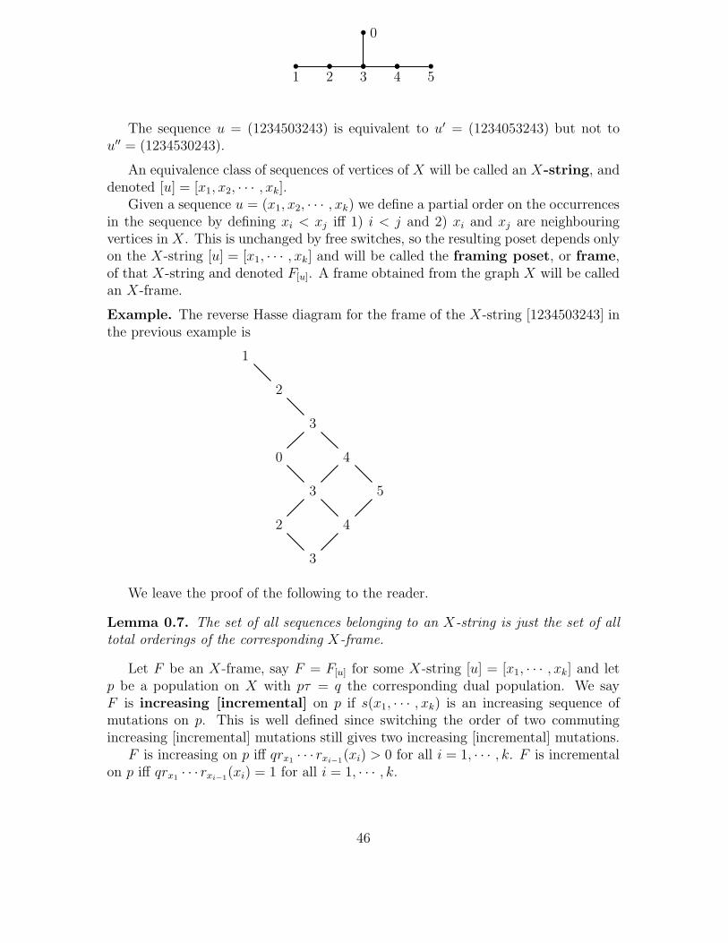
The sequence u = (1234503243) is equivalent to u′ = (1234053243) but not tou′′ = (1234530243).

An equivalence class of sequences of vertices of X will be called an X-string, anddenoted [u] = [x1, x2, · · · , xk].

Given a sequence u = (x1, x2, · · · , xk) we define a partial order on the occurrencesin the sequence by defining xi < xj iff 1) i < j and 2) xi and xj are neighbouringvertices in X. This is unchanged by free switches, so the resulting poset depends onlyon the X-string [u] = [x1, · · · , xk] and will be called the framing poset, or frame,of that X-string and denoted F[u]. A frame obtained from the graph X will be calledan X-frame.

Example. The reverse Hasse diagram for the frame of the X-string [1234503243] inthe previous example is

1

2

3

0 4

3 5

2 4

3

We leave the proof of the following to the reader.

Lemma 0.7. The set of all sequences belonging to an X-string is just the set of alltotal orderings of the corresponding X-frame.

Let F be an X-frame, say F = F[u] for some X-string [u] = [x1, · · · , xk] and letp be a population on X with pτ = q the corresponding dual population. We sayF is increasing [incremental] on p if s(x1, · · · , xk) is an increasing sequence ofmutations on p. This is well defined since switching the order of two commutingincreasing [incremental] mutations still gives two increasing [incremental] mutations.

F is increasing on p iff qrx1 · · · rxi−1(xi) > 0 for all i = 1, · · · , k. F is incremental

on p iff qrx1 · · · rxi−1(xi) = 1 for all i = 1, · · · , k.

46

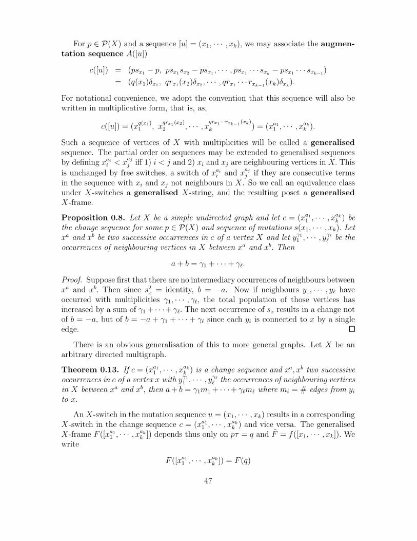
For p ∈ P(X) and a sequence [u] = (x1, · · · , xk), we may associate the augmen-tation sequence A([u])

c([u]) = (psx1 − p, psx1sx2 − psx1 , · · · , psx1 · · · sxk− psx1 · · · sxk−1

)

= (q(x1)δx1 , qrx1(x2)δx2 , · · · , qrx1 · · · rxk−1(xk)δxk

).

For notational convenience, we adopt the convention that this sequence will also bewritten in multiplicative form, that is, as,

c([u]) = (xq(x1)1 , x

qrx1 (x2)2 , · · · , xqrx1 ···rxk−1

(xk)

k ) = (xa11 , · · · , xakk ).

Such a sequence of vertices of X with multiplicities will be called a generalisedsequence. The partial order on sequences may be extended to generalised sequencesby defining xai

i < xaj

j iff 1) i < j and 2) xi and xj are neighbouring vertices in X. This

is unchanged by free switches, a switch of xaii and x

aj

j if they are consecutive termsin the sequence with xi and xj not neighbours in X. So we call an equivalence classunder X-switches a generalised X-string, and the resulting poset a generalisedX-frame.

Proposition 0.8. Let X be a simple undirected graph and let c = (xa11 , · · · , xakk ) be

the change sequence for some p ∈ P(X) and sequence of mutations s(x1, · · · , xk). Letxa and xb be two successive occurrences in c of a vertex X and let yγ11 , · · · , yγ�

� be theoccurrences of neighbouring vertices in X between xa and xb. Then

a+ b = γ1 + · · · + γ�.

Proof. Suppose first that there are no intermediary occurrences of neighbours betweenxa and xb. Then since s2

x = identity, b = −a. Now if neighbours y1, · · · , y� haveoccurred with multiplicities γ1, · · · , γ�, the total population of those vertices hasincreased by a sum of γ1 + · · ·+ γ�. The next occurrence of sx results in a change notof b = −a, but of b = −a + γ1 + · · · + γ� since each yi is connected to x by a singleedge.

There is an obvious generalisation of this to more general graphs. Let X be anarbitrary directed multigraph.

Theorem 0.13. If c = (xa11 , · · · , xakk ) is a change sequence and xa, xb two successive

occurrences in c of a vertex x with yγ11 , · · · , yγ�

� the occurrences of neighbouring verticesin X between xa and xb, then a+ b = γ1m1 + · · ·+ γ�m� where mi = # edges from yito x.

An X-switch in the mutation sequence u = (x1, · · · , xk) results in a correspondingX-switch in the change sequence c = (xa11 , · · · , xak

k ) and vice versa. The generalisedX-frame F ([xa11 , · · · , xak

k ]) depends thus only on pτ = q and F̃ = f([x1, · · · , xk]). Wewrite

F ([xa11 , · · · , xakk ]) = F (q)

47

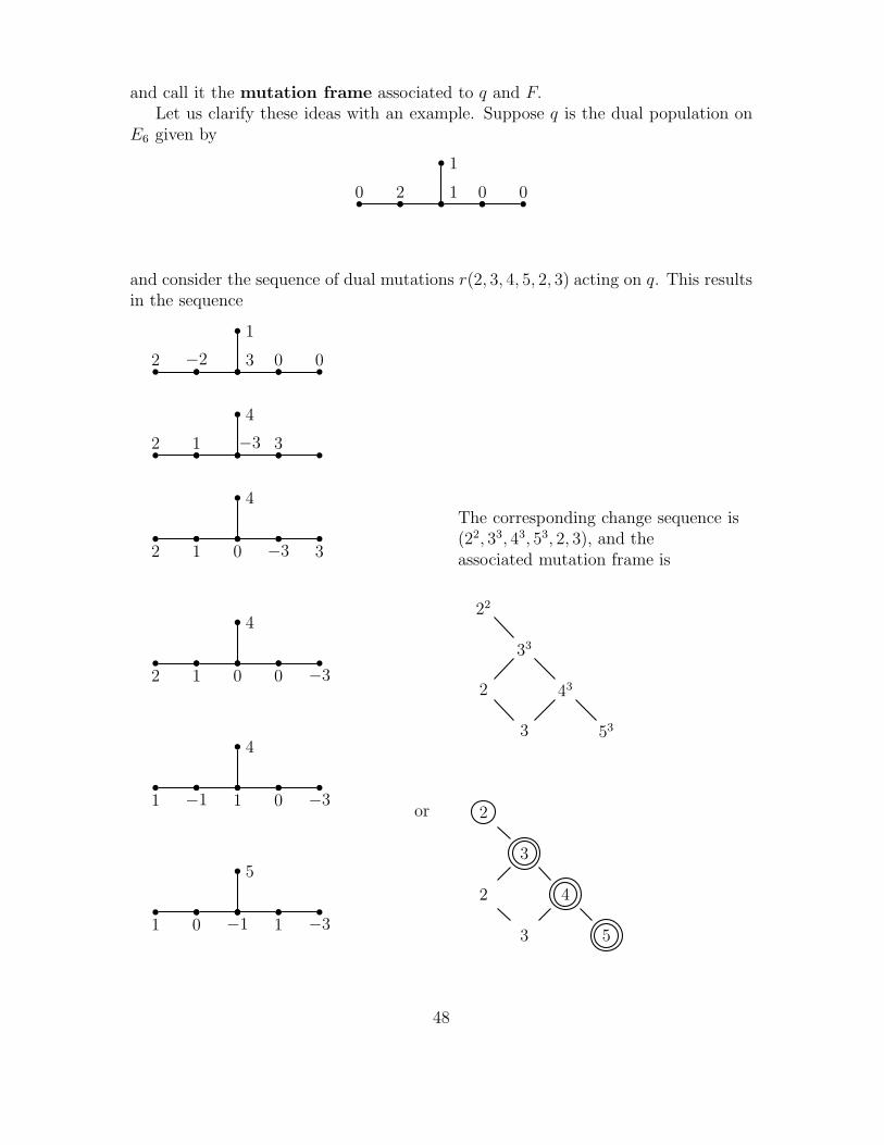
and call it the mutation frame associated to q and F.Let us clarify these ideas with an example. Suppose q is the dual population on

E6 given by

0 2 1 0 0

1

and consider the sequence of dual mutations r(2, 3, 4, 5, 2, 3) acting on q. This resultsin the sequence

2 −2 3 0 0

1

2 1 −3 3

4

2 1 0 −3 3

4

2 1 0 0 −3

4

1 −1 1 0 −3

4

1 0 −1 1 −3

5

The corresponding change sequence is(22, 33, 43, 53, 2, 3), and theassociated mutation frame is

22

33

2 43

3 53

3

2or

2 4

3 5

48

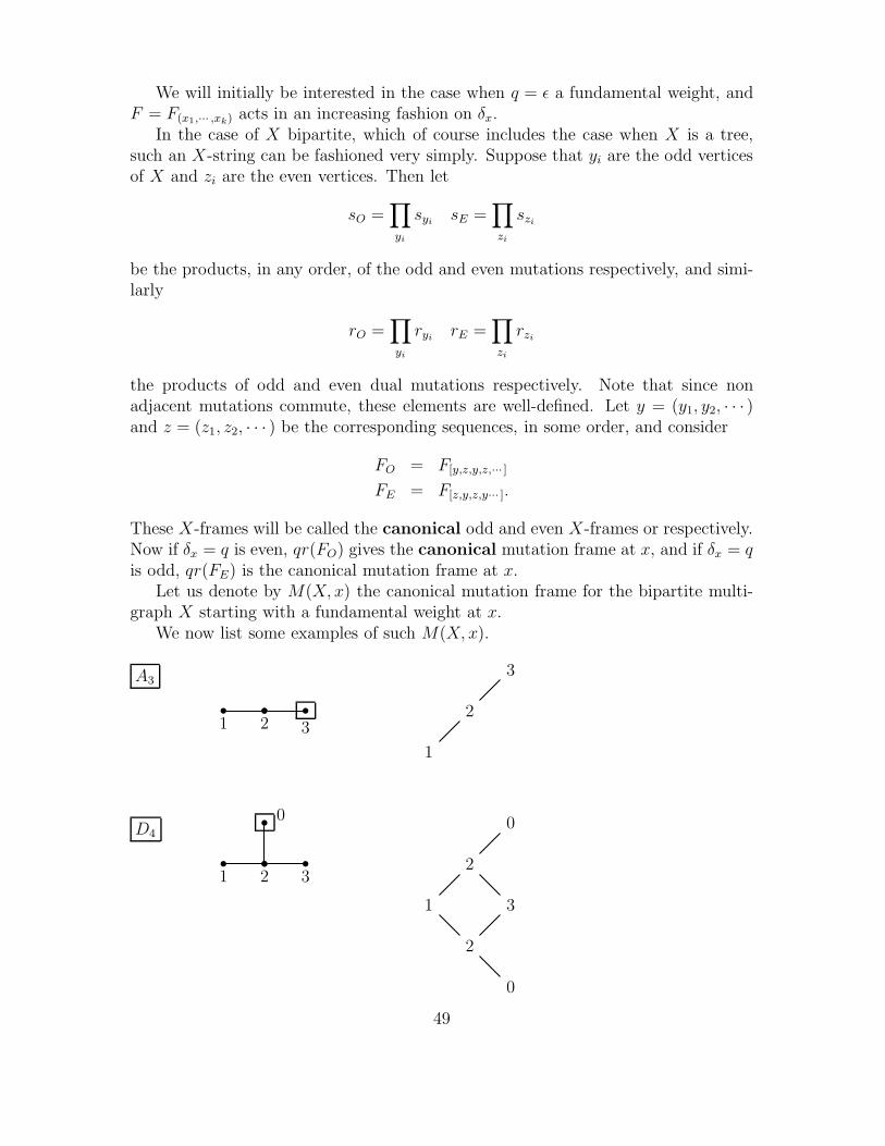
We will initially be interested in the case when q = ε a fundamental weight, andF = F(x1,··· ,xk) acts in an increasing fashion on δx.

In the case of X bipartite, which of course includes the case when X is a tree,such an X-string can be fashioned very simply. Suppose that yi are the odd verticesof X and zi are the even vertices. Then let

sO =∏yi

syisE =

∏zi

szi

be the products, in any order, of the odd and even mutations respectively, and simi-larly

rO =∏yi

ryirE =

∏zi

rzi

the products of odd and even dual mutations respectively. Note that since nonadjacent mutations commute, these elements are well-defined. Let y = (y1, y2, · · · )and z = (z1, z2, · · · ) be the corresponding sequences, in some order, and consider

FO = F[y,z,y,z,··· ]FE = F[z,y,z,y··· ].

These X-frames will be called the canonical odd and even X-frames or respectively.Now if δx = q is even, qr(FO) gives the canonical mutation frame at x, and if δx = qis odd, qr(FE) is the canonical mutation frame at x.

Let us denote by M(X, x) the canonical mutation frame for the bipartite multi-graph X starting with a fundamental weight at x.

We now list some examples of such M(X, x).

A33

2

1

1 2 3

D4

0 0

2

1 3

2

0

1 2 3

49

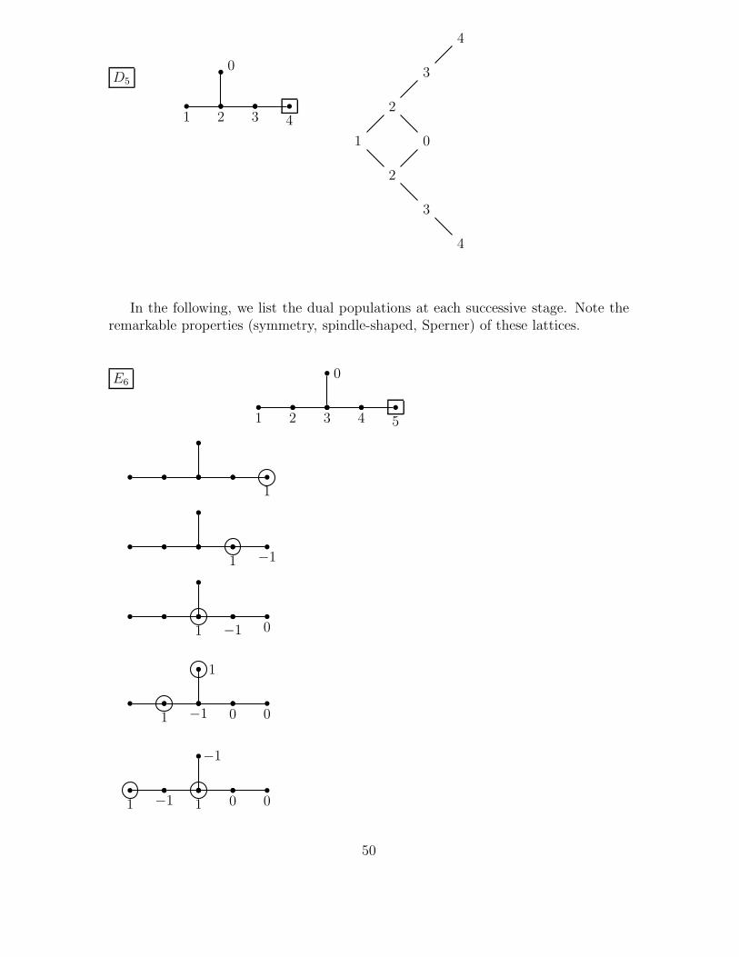
D5

0

1 2 3 4

4

3

2

1 0

2

3

4

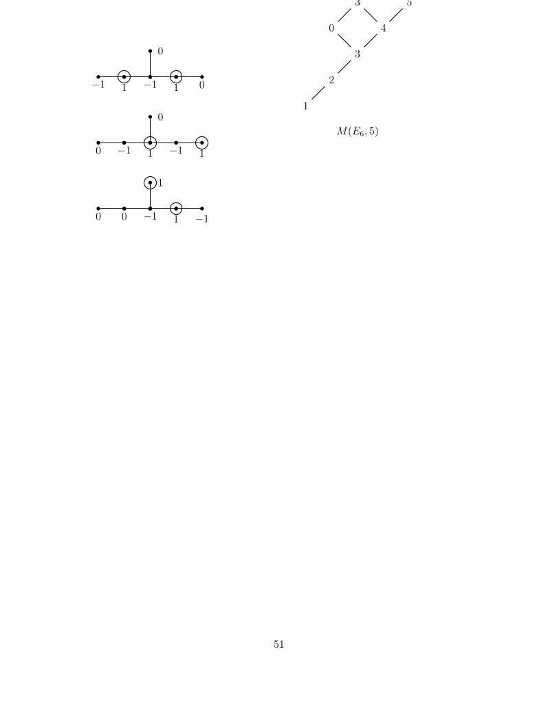
In the following, we list the dual populations at each successive stage. Note theremarkable properties (symmetry, spindle-shaped, Sperner) of these lattices.

E6

1 2 3 4 5

0

1

1 −1

−1 01

0 01

1

−1

01 0−1

−1

1

50

1−1 0−1

0

1

−10 11

0

−1

00 −1−1

1

1

3 5

0 4

3

2

1

M(E6, 5)

51

00 01

−1

−1

10 0−1

0

0

−11 00

0

0

0−1 00

0

0

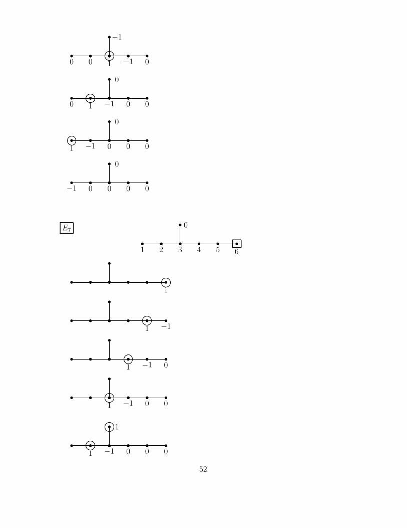
E7

1 2 3 4 5 6

0

1

1 −1

1 −1 0

1 −1 0 0

1 −1 0 0 0

1

52

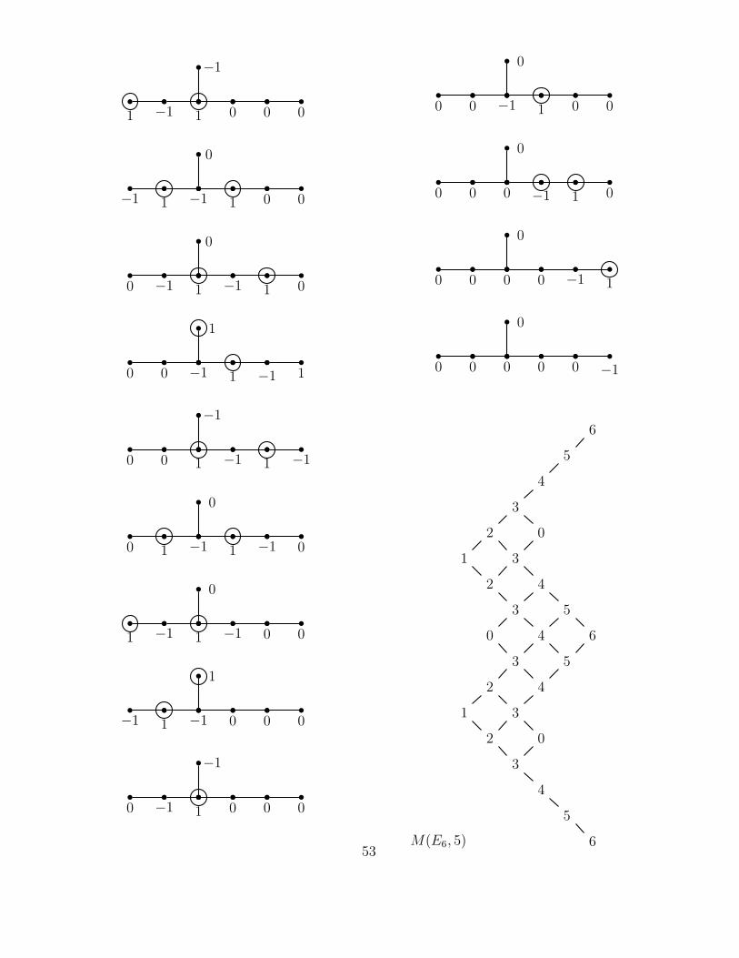
1 −1 1 0 0 0

−1

−1 1 −1 1 0 0

0

0 −1 1 −1 1 0

0

0 0 −1 1 −1 1

1

0 0 1 −1 1 −1

−1

0 1 −1 1 −1 0

0

1 −1 1 −1 0 0

0

−1 1 −1 0 0 0

1

0 −1 1 0 0 0

−1

0 0 −1 1 0 0

0

0 0 0 −1 1 0

0

0 0 0 0 −1 1

0

0 0 0 0 0 −1

0

6

5

4

3

2 0

1 3

2 4

3 5

0 4 6

3 5

2 4

1 3

2 0

3

4

5

6M(E6, 5)53

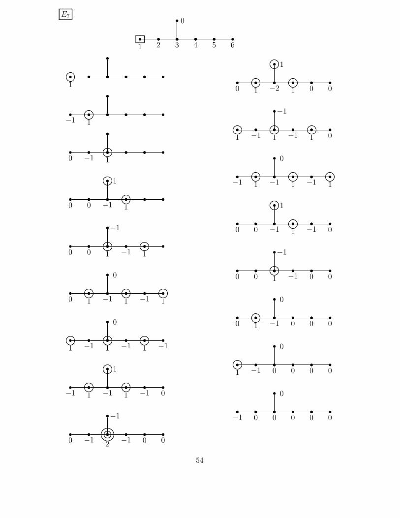
E7

1 2 3 4 5 6

0

1

−1 1

0 −1 1

0 0 −1 1

1

0 0 1 −1 1

−1

0 1 −1 1 −1 1

0

1 −1 1 −1 1 −1

0

−1 1 −1 1 −1 0

1

0 −12

−1 0 0

−1

0 1 −2 1 0 0

1

1 −1 1 −1 1 0

−1

−1 1 −1 1 −1 1

0

0 0 −1 1 −1 0

1

0 0 1 −1 0 0

−1

0 1 −1 0 0 0

0

1 −1 0 0 0 0

0

−1 0 0 0 0 0

0

54

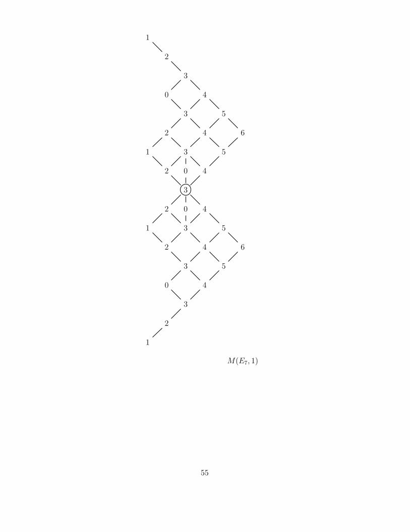
1

2

3

0 4

3 5

2 4 6

1 3 5

2 0 4

3

2 0 4

1 3 5

2 4 6

3 5

0 4

3

2

1

M(E7, 1)

55

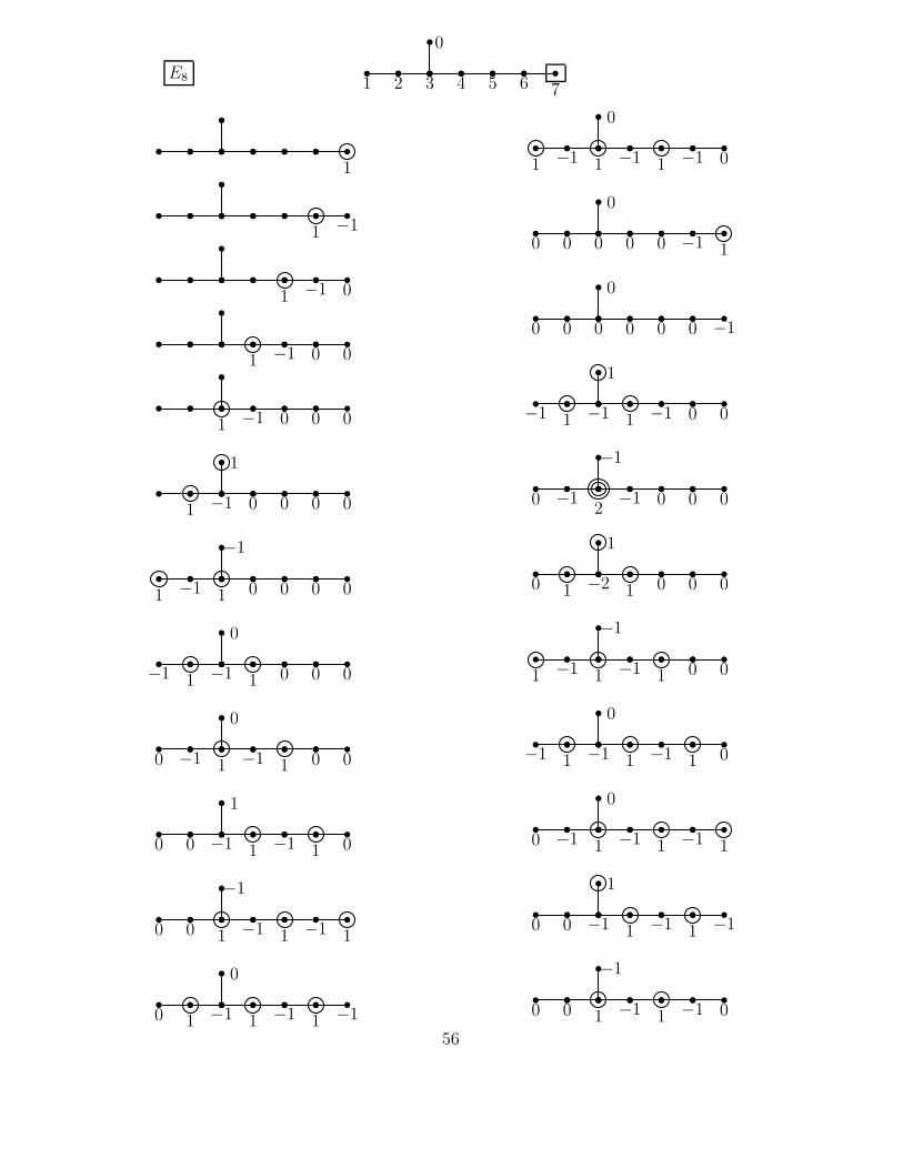
E8 1 2 3 4 5 6 7

0

1

1 −1

1 −1 0

1 −1 0 0

1 −1 0 0 0

1 −1 0 0 0 0

1

1 −1 1 0 0 0 0

−1

−1 1 −1 1 0 0 0

0

0 −1 1 −1 1 0 0

0

0 0 −1 1 −1 1 0

1

0 0 1 −1 1 −1 1

−1

0 1 −1 1 −1 1 −1

0

1 −1 1 −1 1 −1 0

0

0 0 0 0 0 −1 1

0

0 0 0 0 0 0 −1

0

−1 1 −1 1 −1 0 0

1

0 −12

−1 0 0 0

−1

0 1 −2 1 0 0 0

1

1 −1 1 −1 1 0 0

−1

−1 1 −1 1 −1 1 0

0

0 −1 1 −1 1 −1 1

0

0 0 −1 1 −1 1 −1

1

0 0 1 −1 1 −1 0

−1

56

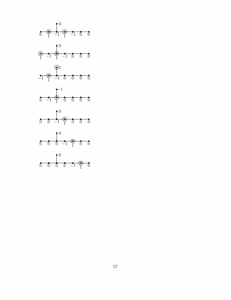
0 1 −1 1 −1 0 0

0

1 −1 1 −1 0 0 0

0

−1 1 −1 0 0 0 0

1

0 −1 1 0 0 0 0

−1

0 0 −1 1 0 0 0

0

0 0 0 −1 1 0 0

0

0 0 0 0 −1 1 0

0

57

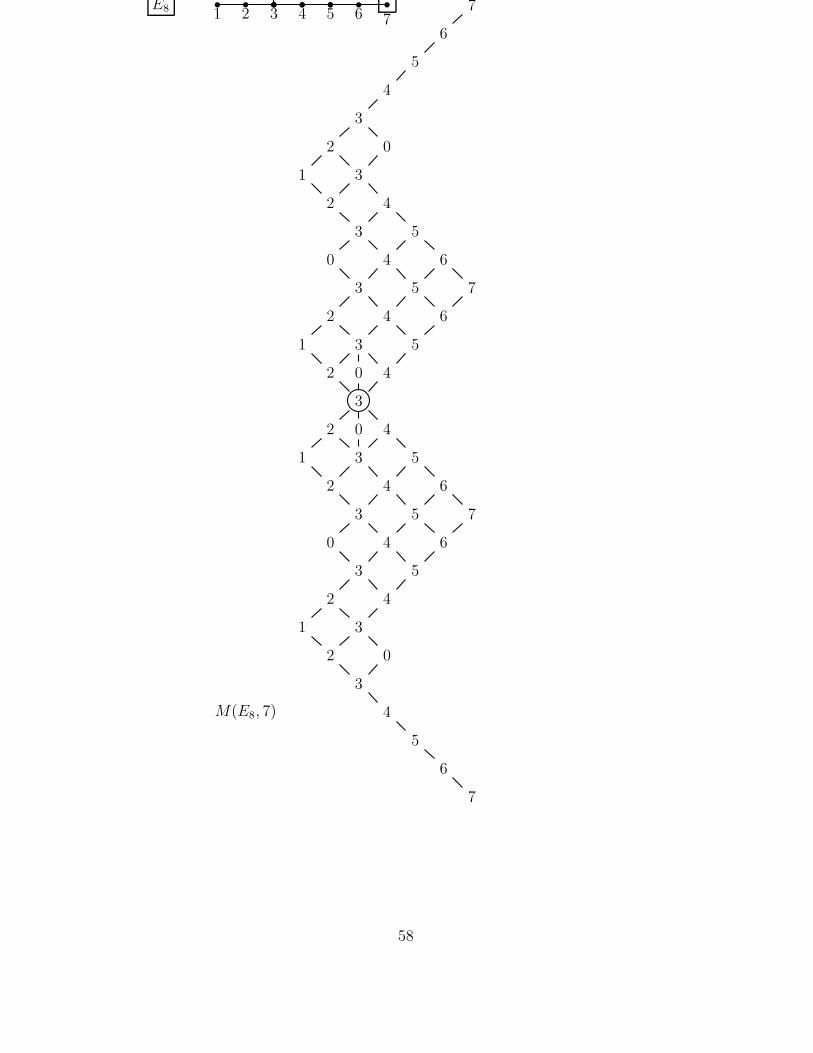
E8 1 2 3 4 5 6 77

6

5

4

3

2 0

1 3

2 4

3 5

0 4 6

3 5 7

2 4 6

1 3 5

2 0 4

3

2 0 4

1 3 5

2 4 6

3 5 7

0 4 6

3 5

2 4

1 3

2 0

3

4

5

6

7

M(E8, 7)

58

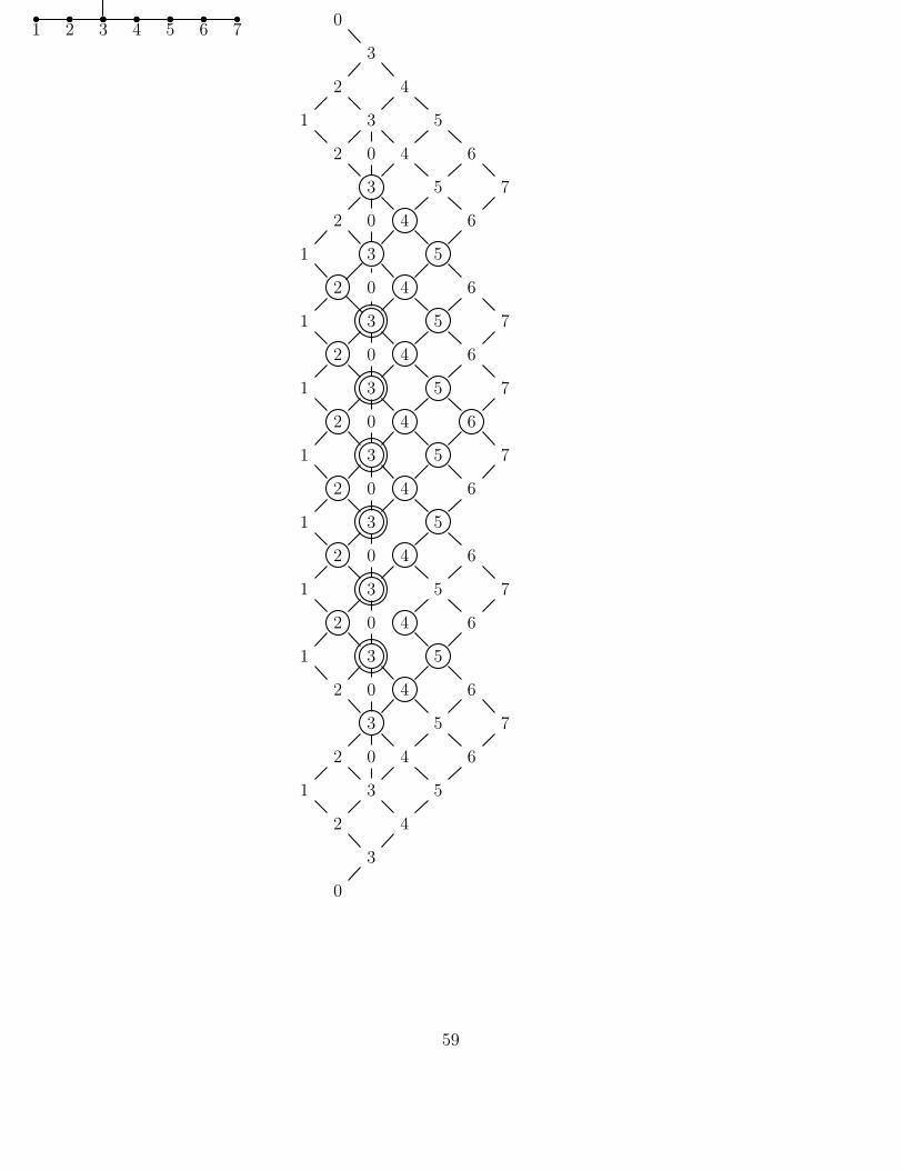
1 2 3 4 5 6 70

3

2 4

1 3 5

2 0 4 6

3 5 7

2 0 4 6

1 3 5

2 0 4 6

1 3 5 7

2 0 4 6

1 3 5 7

2 0 4 6

1 3 5 7

2 0 4 6

1 3 5

2 0 4 6

1 3 5 7

2 0 4 6

1 3 5

2 0 4 6

3 5 7

2 0 4 6

1 3 5

2 4

3

0

59

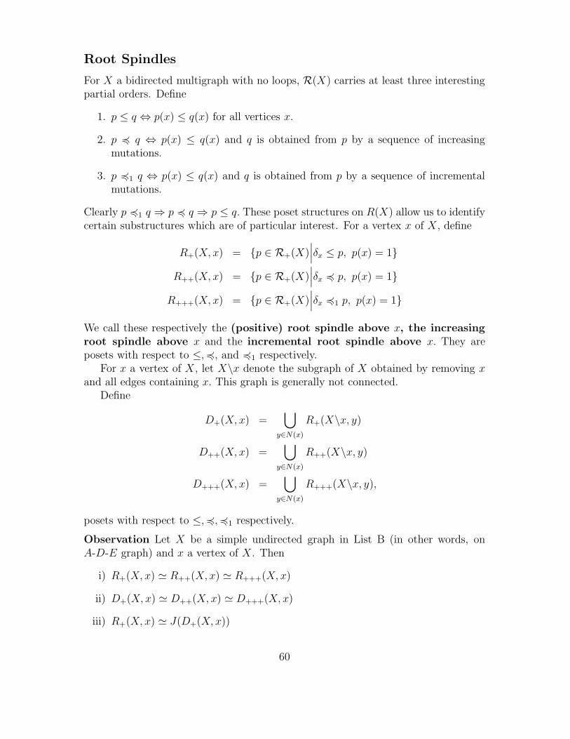
Root Spindles

For X a bidirected multigraph with no loops, R(X) carries at least three interestingpartial orders. Define

1. p ≤ q ⇔ p(x) ≤ q(x) for all vertices x.

2. p � q ⇔ p(x) ≤ q(x) and q is obtained from p by a sequence of increasingmutations.

3. p �1 q ⇔ p(x) ≤ q(x) and q is obtained from p by a sequence of incrementalmutations.

Clearly p �1 q ⇒ p � q ⇒ p ≤ q. These poset structures on R(X) allow us to identifycertain substructures which are of particular interest. For a vertex x of X, define

R+(X, x) = {p ∈ R+(X)∣∣∣δx ≤ p, p(x) = 1}

R++(X, x) = {p ∈ R+(X)∣∣∣δx � p, p(x) = 1}

R+++(X, x) = {p ∈ R+(X)∣∣∣δx �1 p, p(x) = 1}

We call these respectively the (positive) root spindle above x, the increasingroot spindle above x and the incremental root spindle above x. They areposets with respect to ≤,�, and �1 respectively.

For x a vertex of X, let X\x denote the subgraph of X obtained by removing xand all edges containing x. This graph is generally not connected.

Define

D+(X, x) =⋃

y∈N(x)

R+(X\x, y)

D++(X, x) =⋃

y∈N(x)

R++(X\x, y)

D+++(X, x) =⋃

y∈N(x)

R+++(X\x, y),

posets with respect to ≤,�,�1 respectively.

Observation Let X be a simple undirected graph in List B (in other words, onA-D-E graph) and x a vertex of X. Then

i) R+(X, x) � R++(X, x) � R+++(X, x)

ii) D+(X, x) � D++(X, x) � D+++(X, x)

iii) R+(X, x) � J(D+(X, x))

60

The graphs in the Observation are all trees and it is readily seen that since anysubgraph which is connected is also of this form, the case when x is an endpoint ofX is the crucial situation.

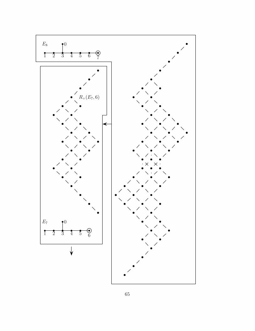
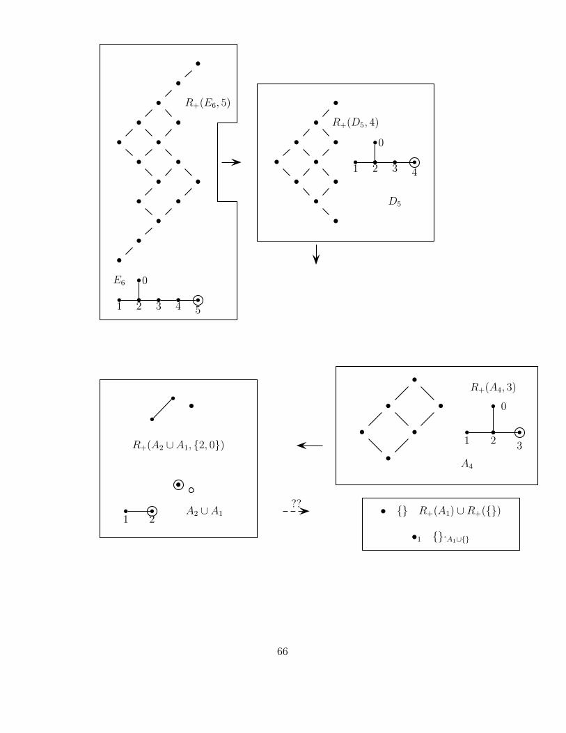
It follows that the root spindles of the A-D-E graphs exhibit a remarkable induc-tive or ‘cascading’ structure which links them all together in the following pattern.

A1

↑A2

↑A3

↑A4

↑A5

↑A6

↑A7

↑A8

↑A9

...

D4

↑D5

↑D6

↑D7

↑D8

↑D9

...

E6

↑E7

↑E8

From this diagram, the poset structures of the various root spindles can be builtup, once one understands the isomorphism in part iii) of the Observation. For thiswe need to connect root spindles to mutation frames, and the key tool is the comple-mentation map ψ. It then will be seen that the inductive cascading shown above isbut a special case of a much more general phenomenon.

61

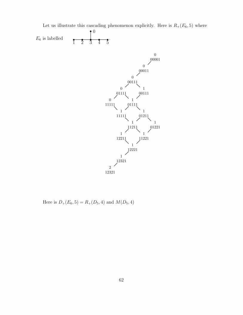
Let us illustrate this cascading phenomenon explicitly. Here is R+(E6, 5) where

E6 is labelled1 2 3 4 5

0

.

000001

000011

000111

001111

100111

011111

101111

111111

101211

111211

101221

112211

111221

112221

112321

212321

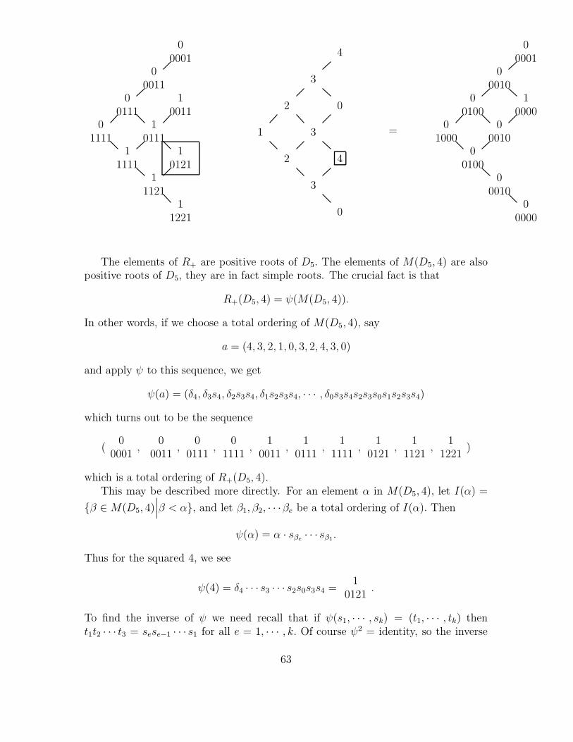
Here is D+(E6, 5) = R+(D5, 4) and M(D5, 4)

62

00001

00011

00111

10011

01111

10111

11111

10121

11121

11221

4

3

2 0

1 3

2 4

3

0

=

00001

00010

00100

10000

01000

00010

00100

00010

00000

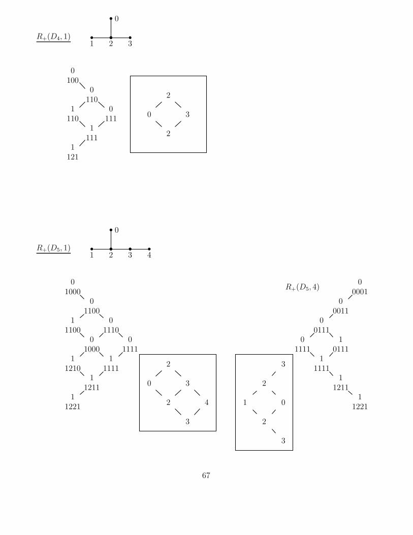
The elements of R+ are positive roots of D5. The elements of M(D5, 4) are alsopositive roots of D5, they are in fact simple roots. The crucial fact is that

R+(D5, 4) = ψ(M(D5, 4)).

In other words, if we choose a total ordering of M(D5, 4), say

a = (4, 3, 2, 1, 0, 3, 2, 4, 3, 0)

and apply ψ to this sequence, we get

ψ(a) = (δ4, δ3s4, δ2s3s4, δ1s2s3s4, · · · , δ0s3s4s2s3s0s1s2s3s4)

which turns out to be the sequence

(0

0001,

00011

,0

0111,

01111

,1

0011,

10111

,1

1111,

10121

,1

1121,

11221

)

which is a total ordering of R+(D5, 4).This may be described more directly. For an element α in M(D5, 4), let I(α) =

{β ∈M(D5, 4)∣∣∣β < α}, and let β1, β2, · · ·βe be a total ordering of I(α). Then

ψ(α) = α · sβe · · · sβ1.

Thus for the squared 4, we see

ψ(4) = δ4 · · · s3 · · · s2s0s3s4 =1

0121.

To find the inverse of ψ we need recall that if ψ(s1, · · · , sk) = (t1, · · · , tk) thent1t2 · · · t3 = sese−1 · · · s1 for all e = 1, · · · , k. Of course ψ2 = identity, so the inverse

63

of ψ is itself. Thus

ψ−1(1

0121) = ψ(

10121

) =1

0121· · · s

10111

s0

0111

s1

0011

s0

0011

s0

0001

but this formula involves non-simple reflections. Using the identity and assuming

ψ−1(γ) has been found for all γ ∈ I(1

0121), we may see that if I(

10121

) has

ordering s1, s2, · · · se, then

ψ(1

0121) =

10121

· sψ(s1)sψ(s2) · · · sψ(se).

In our case this becomes

ψ−1(1

0121) =

10121

· s4s3s2s1s3 =1

0001= .

These observations generalise.Observation Let X be a simple undirected graph in List B (an A-D-E graph) andx an extreme vertex of X. Then

i) R+(X, x) � M(X, x) and the isomorphism is given by the complementationmap ψ.

ii) If α ∈ M(X, x) and β1, · · · , βe a total ordering of the ideal I(α) = {β < α} inM(X, x) then ψ(α) = α · sβe · · · sβ1 .

iii) If γ ∈ R+(X, x) and δ1, · · · , δe a total ordering of the ideal I(γ) = {δ < γ} inR+(X, x) then

ψ(γ) = γsψ(δ1) · · · sψ(δe)

64

1 2 3 4 5 6 7

0E8 ••

••

•• •

• •• •

• •• • •

• • •• • •

• • •• • •• • •

• • •• • •

• • •• • •

• •• •

• •• •

••

••

••

••

• •• •

• •• •

• • •• •

• •• •

• ••

••

•

1 2 3 4 5 6

0E7

R+(E7, 6)

65

1 2 3 4 5

0E6

••

•• •

• •• •

• •• •

••

•

R+(E6, 5) ••

• •• •

•••

•

R+(D5, 4)

1 2 3 4

0

D5

1 2A2 ∪ A1

•

R+(A2 ∪A1, {2, 0})

•

•

•

•

•

•

•

R+(A4, 3)

0

1 2 3

A4

• {} R+(A1) ∪ R+({})

•1 {}·A1∪{}

??

66

1 2 3

0

R+(D4, 1)

0100

0110

1110

0111

1111

1121

2

0 3

2

1 2 3

0

4R+(D5, 1)

01000

01100

11100

01110

01000

01111

11210

11111

11211

11221

00001

00011

00111

01111

10111

11111

11211

11221

R+(D5, 4)

2

0 3

2 4

3

3

2

1 0

2

3

67

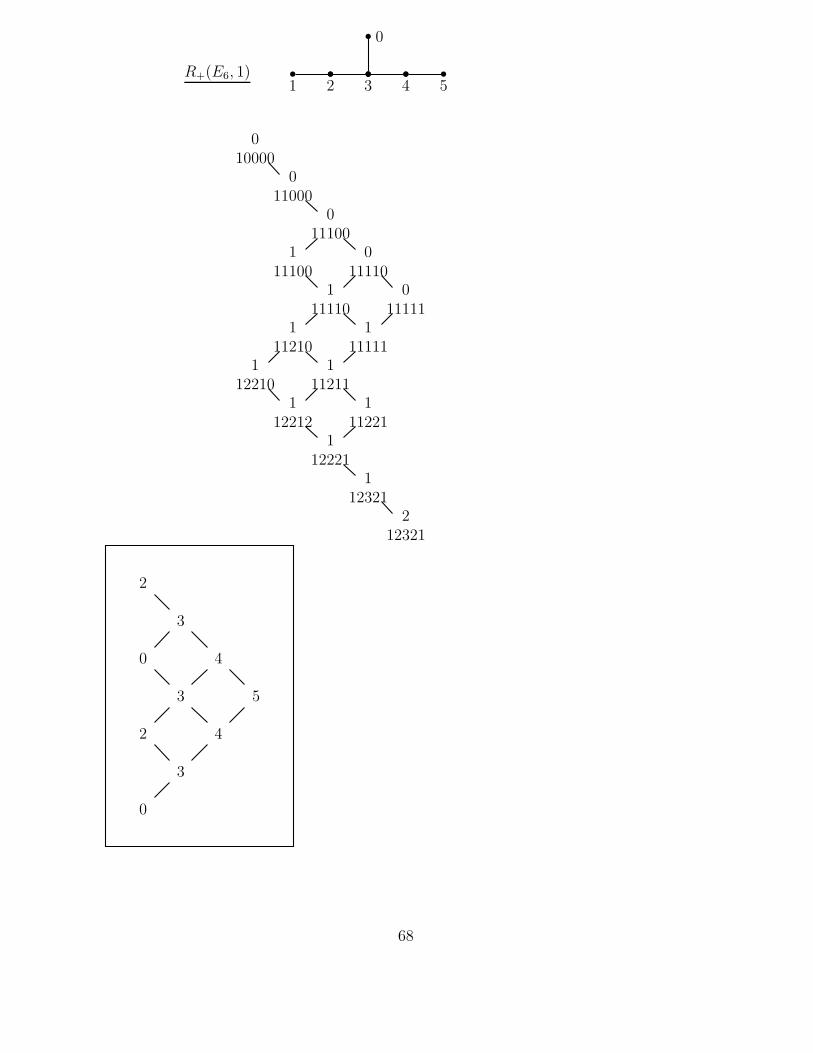
1 2 3 4 5

0

R+(E6, 1)

010000

011000

011100

111100

011110

111110

011111

111210

111111

112210

111211

112212

111221

112221

112321

212321

2

3

0 4

3 5

2 4

3

0

68

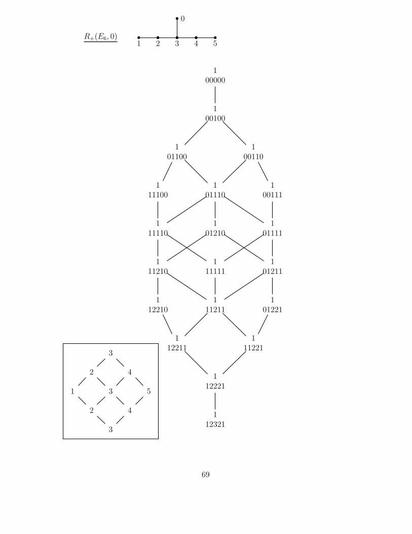
1 2 3 4 5

0

R+(E6, 0)

100000

100100

101100

100110

111100

101110

100111

111110

101210

101111

111210

111111

101211

112210

111211

101221

112211

111221

112221

112321

3

2 4

1 3 5

2 4

3

69

1 2 3 4 5 6

0R+(E7, 6)

0000001

0000011

0000111

0001111

0011111

1001111

0111111

1011111

1111111

1012111

1112111

1012211

1122111

1112211

1012221

1122211

1112221

1123211

1122221

2123211

1123221

2123221

1123321

2123321

2124321

2134321

2234321

5

4

3

2 0

1 3

2 4

3 5

0 4

3

2

1

70

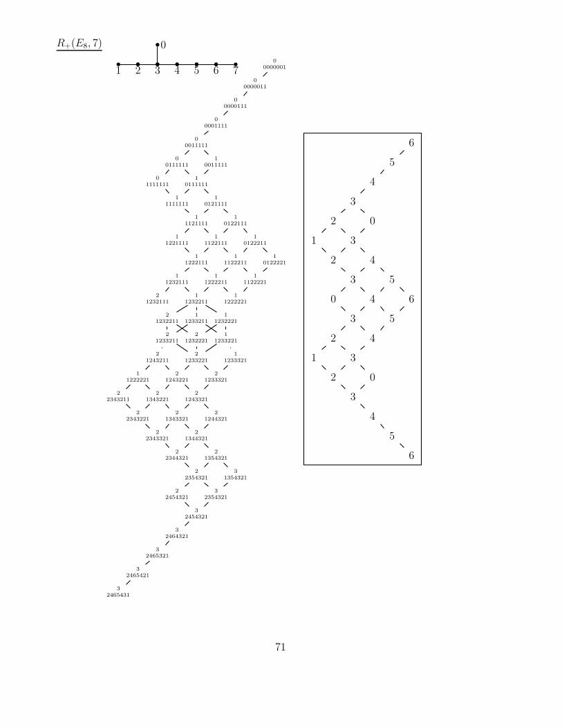
1 2 3 4 5 6 7

0R+(E8, 7)

00000001

00000011

00000111

00001111

00011111

00111111

10011111

01111111

10111111

11111111

10121111

11121111

10122111

11221111

11122111

10122211

11222111

11122211

10122221

11232111

11222211

11122221

21232111

11232211

11222221

21232211

11233211

11232221

21233211

21232221

11233221

21243211

21233221

11233321

11222221

21243221

21233321

22343211

21343221

21243321

22343221

21343321

21244321

22343321

21344321

22344321

21354321

22354321

31354321

22454321

32354321

32454321

32464321

32465321

32465421

32465431

6

5

4

3

2 0

1 3

2 4

3 5

0 4 6

3 5

2 4

1 3

2 0

3

4

5

6

71

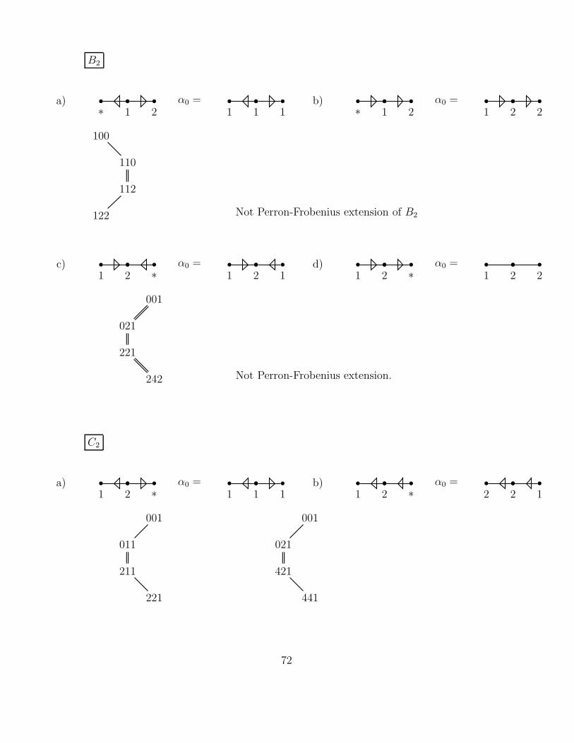
B2

∗ 1 2a)

1 1 1α0 =

∗ 1 2b)

1 2 2α0 =

100

110

112

122 Not Perron-Frobenius extension of B2

1 2 ∗c)

1 2 1α0 =

1 2 ∗d)

1 2 2α0 =

001

021

221

242 Not Perron-Frobenius extension.

C2

1 2 ∗a)

1 1 1α0 =

1 2 ∗b)

2 2 1α0 =

001

011

211

221

001

021

421

441

72

∗ 1 2c)

1 2 1α0 =

∗ 1 2d)

2 2 1α0 =

100

120

122

142

100

110

111

121

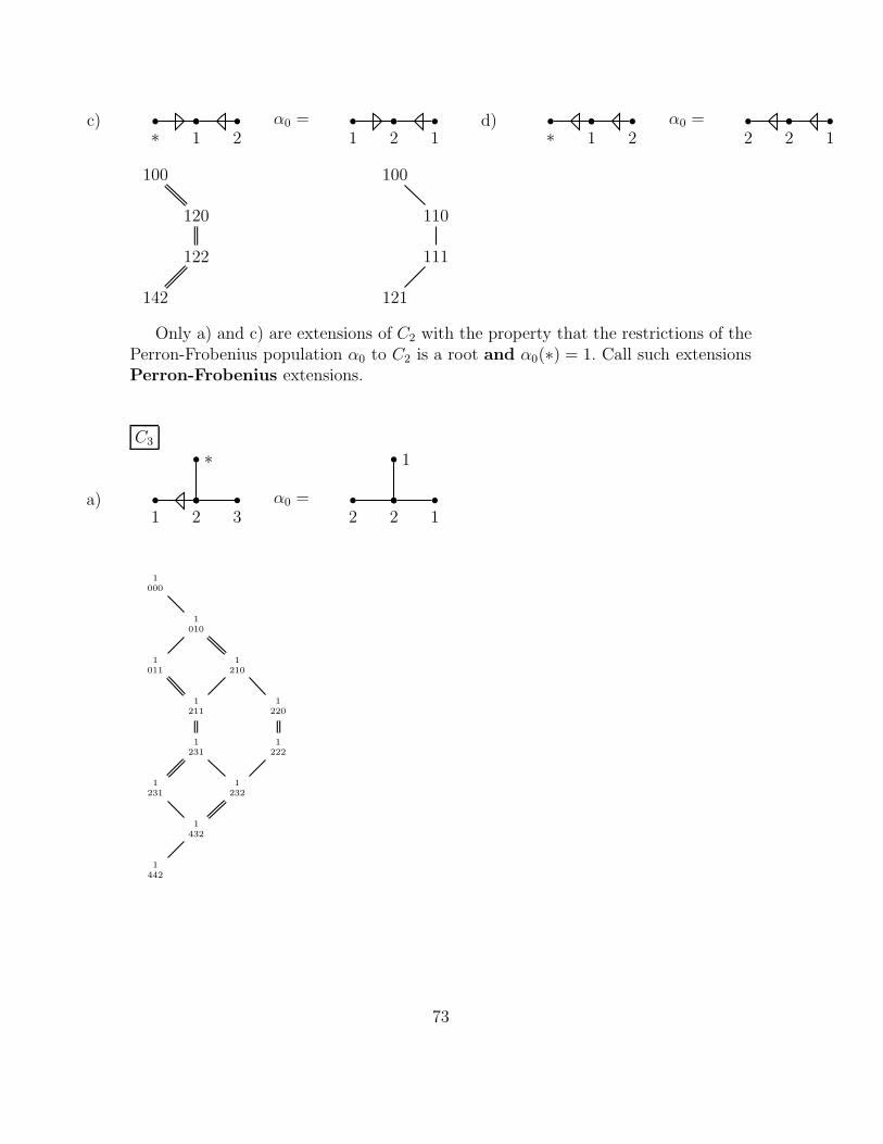
Only a) and c) are extensions of C2 with the property that the restrictions of thePerron-Frobenius population α0 to C2 is a root and α0(∗) = 1. Call such extensionsPerron-Frobenius extensions.

C3

1 2 3

∗

a)2 2 1

1

α0 =

1000

1010

1011

1210

1211

1220

1231

1222

1231

1232

1432

1442

73

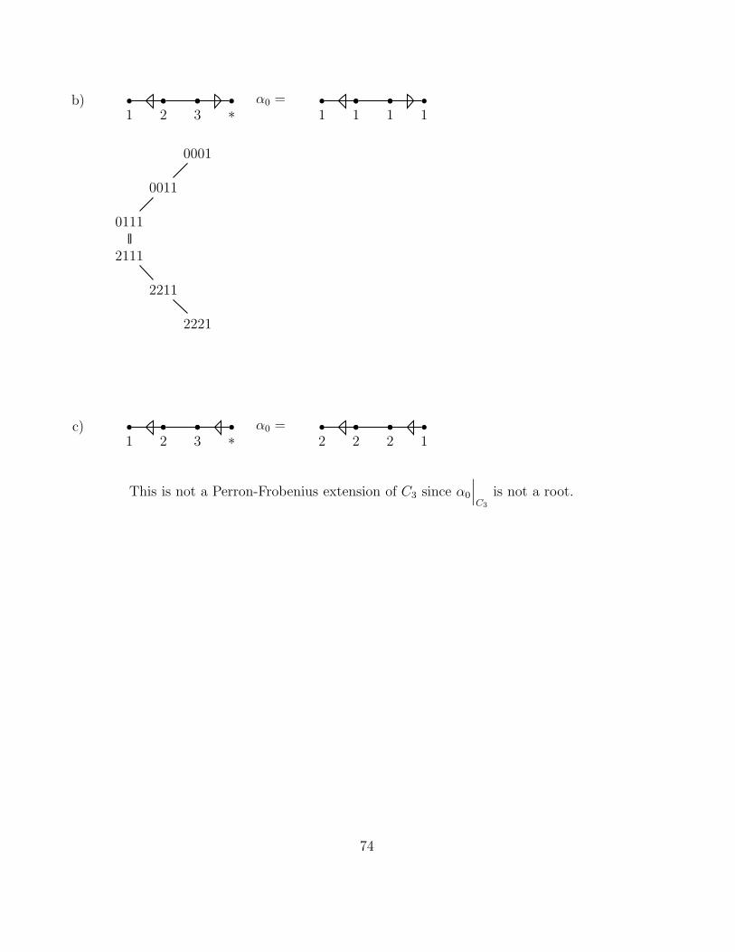
1 2 3 ∗b)

1 1 1 1α0 =

0001

0011

0111

2111

2211

2221

1 2 3 ∗c)

2 2 2 1α0 =

This is not a Perron-Frobenius extension of C3 since α0

∣∣∣C3

is not a root.

74

D4

1 2 3

0

∗1 2 1

1

1

α0 =

00001

00101

01101

10101

00111

11101

01111

10111

11201

01211

11111

10211

11221

2121 1

11311

12211

11321

21311

12311

21321

12321

22311

22321

22421

75

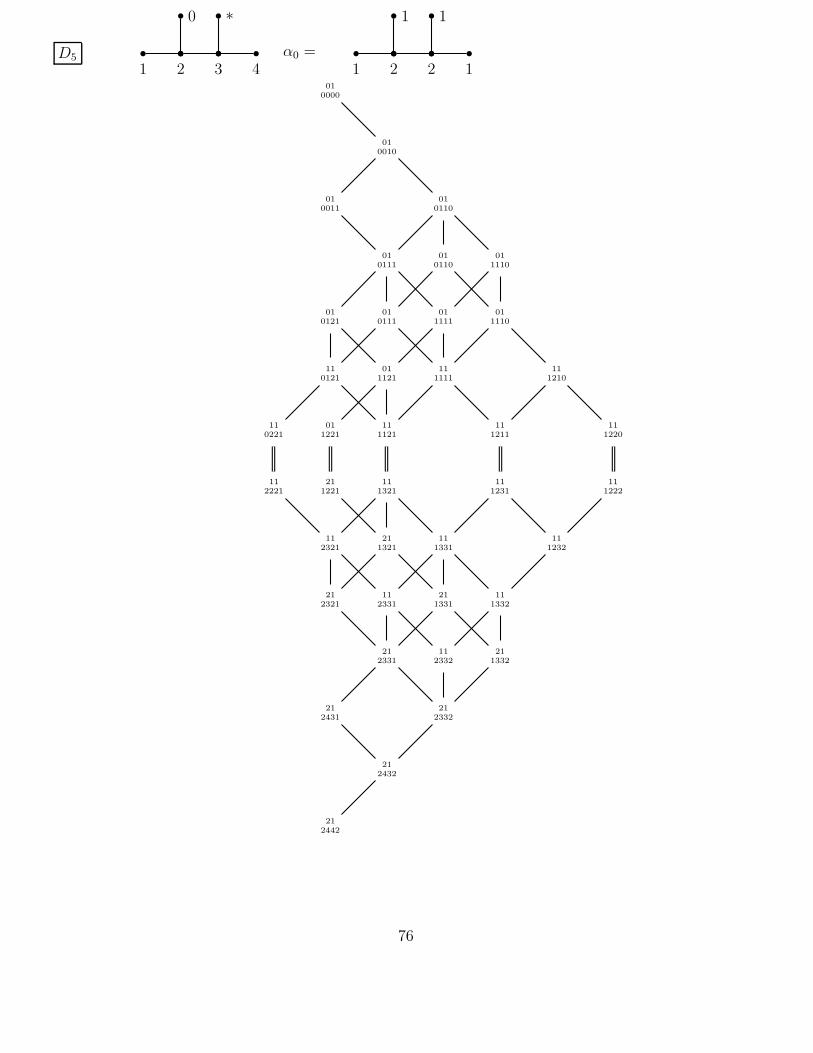
D5

1 2 3 4

0 ∗

1 2 2 1

1 1

α0 =

010000

010010

010011

010110

010111

010110

011110

010121

010111

011111

011110

110121

011121

111111

111210

110221

011221

111121

111211

111220

112221

211221

111321

111231

111222

112321

211321

111331

111232

212321

112331

211331

111332

212331

112332

211332

212431

212332

212432

212442

76

• •

•

10 0

−11 1

0−1 2

02 − 1

21 − 2

2−2 1

−23 0

3−1 − 1

−20 3

1−3 3

−32 2

13 − 3

40 − 3

−1−2 4

−14 − 2

4−3 0

−44 1

32 − 4

3−4 2

−41 4

5 5 5 5 5

0−4 5

−35 − 1

5−2 − 2

−3−1 5

05 − 4

51 − 5

2−5 4

−53 3

24 − 5

5−5 1

−56 0

6−1 − 4

−2−3 6

−26 − 3

6−4 − 1

−50 6

55

6 6 6 6 6 6

1−6 6

−65 2

43 − 6

4−6 3

−62 5

16 − 6

1 5 2 4 3 3 4 2 5

70 − 6

−1−5 7

−47 − 2

7−3 − 3

−4−2 7

−17 − 5

7−6 0

7 7 7 7 7 7 7

−77 1

62 − 7

3−7 5

−74 4

35 − 7

6−7 2

−71 7

......

......

......

...

77

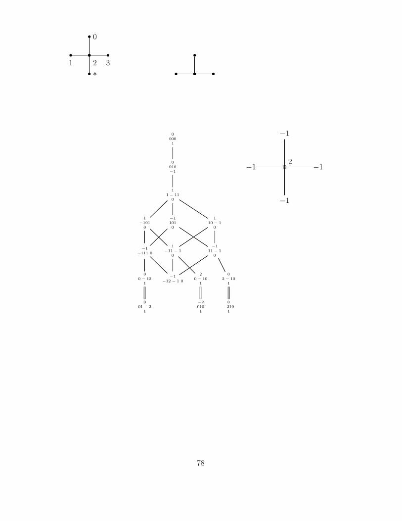
1 2 3

0

∗

00001

0010−1

11 − 11

0

1−101

0

−11010

110 − 1

0

−1−111 0

1−11 − 1

0

−111 − 1

0

00 − 12

1

−1−12 − 1 0

20 − 10

1

02 − 10

1

001 − 2

1

−20101

0−210

1

−1

−1

−1 −12

78

• •

•

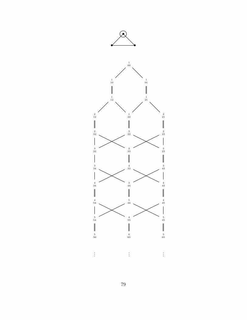
100

110

101

112

121

212

122

221

232

322

223

332

233

323

334

433

343

434

344

443

454

544

445

554

455

545

556

665

565

......

...

79