CD Tutorial 4The MODI and VAMMethods of SolvingTransportation ProblemsTutorial Outline

MODI METHOD

How to Use the MODI Method

Solving the Arizona Plumbing Problem withMODI

VOGEL’S APPROXIMATION METHOD:ANOTHER WAY TO FIND AN INITIALSOLUTION

DISCUSSION QUESTIONS

PROBLEMS

T4-2 CD TU TO R I A L 4 TH E MODI A N D VAM ME T H O D S O F SO LV I N G TR A N S P O RTAT I O N PRO B L E M S

This tutorial deals with two techniques for solving transportation problems: the MODI method andVogel’s Approximation Method (VAM).

MODI METHODThe MODI (modified distribution) method allows us to compute improvement indices quickly foreach unused square without drawing all of the closed paths. Because of this, it can often provideconsiderable time savings over other methods for solving transportation problems.

MODI provides a new means of finding the unused route with the largest negative improvementindex. Once the largest index is identified, we are required to trace only one closed path. This pathhelps determine the maximum number of units that can be shipped via the best unused route.

How to Use the MODI MethodIn applying the MODI method, we begin with an initial solution obtained by using the northwest cor-ner rule or any other rule. But now we must compute a value for each row (call the values R1, R2, R3 ifthere are three rows) and for each column (K1, K2, K3 ) in the transportation table. In general, we let

The MODI method then requires five steps:

1. To compute the values for each row and column, set

Ri + Kj = Cij

but only for those squares that are currently used or occupied. For example, if the square atthe intersection of row 2 and column 1 is occupied, we set R2 + K1 = C21.

2. After all equations have been written, set R1 = 0.3. Solve the system of equations for all R and K values.4. Compute the improvement index for each unused square by the formula improvement

index (Iij) = Cij � Ri � Kj.5. Select the largest negative index and proceed to solve the problem as you did using the

stepping-stone method.

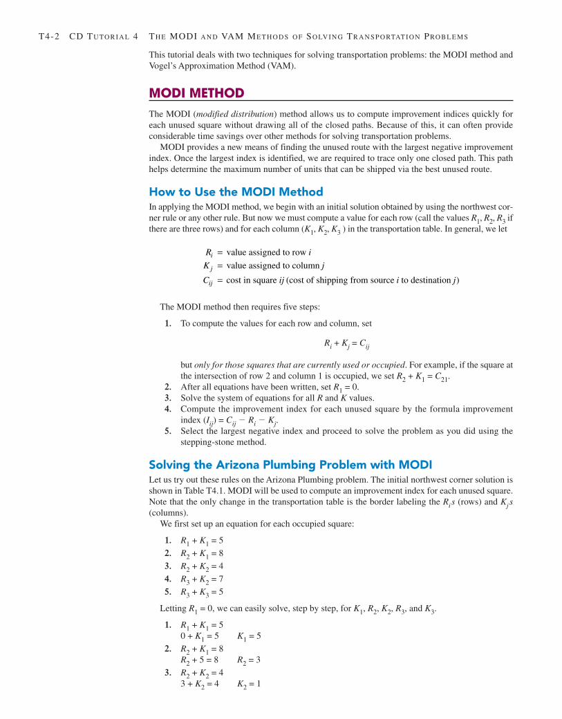
Solving the Arizona Plumbing Problem with MODILet us try out these rules on the Arizona Plumbing problem. The initial northwest corner solution isshown in Table T4.1. MODI will be used to compute an improvement index for each unused square.Note that the only change in the transportation table is the border labeling the Ris (rows) and Kjs(columns).

We first set up an equation for each occupied square:

1. R1 + K1 = 5

2. R2 + K1 = 8

3. R2 + K2 = 4

4. R3 + K2 = 7

5. R3 + K3 = 5

Letting R1 = 0, we can easily solve, step by step, for K1, R2, K2, R3, and K3.

1. R1 + K1 = 50 + K1 = 5 K1 = 5

2. R2 + K1 = 8R2 + 5 = 8 R2 = 3

3. R2 + K2 = 43 + K2 = 4 K2 = 1

R i

K j

C ij i j

i

j

ij

===

value assigned to row

value assigned to column

cost in square (cost of shipping from source to destination )

MODI ME T H O D T4-3

TABLE T4.1

Initial Solution to ArizonaPlumbing Problem in theMODI Format

FROM

TOALBUQUERQUE BOSTON CLEVELAND

FACTORYCAPACITY

DES MOINES

EVANSVILLE

FORTLAUDERDALE

WAREHOUSEREQUIREMENTS

5

8

4 3100

Kj

Ri

R1

R2

R3

K1 K2 K3

200

200 300

100

100

300

100

4 3

9 7 5

700200300 200

4. R3 + K2 = 7R2 + 1 = 7 R3 = 6

5. R3 + K3 = 56 + K3 = 5 K3 = �1

You can observe that these R and K values will not always be positive; it is common for zero and neg-ative values to occur as well. After solving for the Rs and Ks in a few practice problems, you may becomeso proficient that the calculations can be done in your head instead of by writing the equations out.

The next step is to compute the improvement index for each unused cell. That formula is

improvement index = Iij = Cij � Ri � Kj

We have:

Because one of the indices is negative, the current solution is not optimal. Now it is necessary totrace only the one closed path, for Fort Lauderdale–Albuquerque, in order to proceed with the solu-tion procedures.

The steps we follow to develop an improved solution after the improvement indices have beencomputed are outlined briefly:

1. Beginning at the square with the best improvement index (Fort Lauderdale–Albuquerque),trace a closed path back to the original square via squares that are currently being used.

2. Beginning with a plus (+) sign at the unused square, place alternate minus (�) signs andplus signs on each corner square of the closed path just traced.

3. Select the smallest quantity found in those squares containing minus signs. Add that num-ber to all squares on the closed path with plus signs; subtract the number from all squaresassigned minus signs.

4. Compute new improvement indices for this new solution using the MODI method.

Des Moines–Boston index (or

Des Moines–Cleveland index (or

Evansville–Cleveland index (or

Fort Lauderdale–Albuquerque index (or

= = − − = − −= += = − − = − − −= += = − − = − − −= += = − −

I I C R K

I I C R K

I I C R K

I I C R

DB

DC

EC

FA

12 12 1 2

13 13 1 3

23 23 2 3

31 31 3

4 0 1

3

3 0 1

4

3 3 1

1

)

$

) ( )

$

) ( )

$

) KK1 9 6 5

2

= − −= −$

T4-4 CD TU TO R I A L 4 TH E MODI A N D VAM ME T H O D S O F SO LV I N G TR A N S P O RTAT I O N PRO B L E M S

TABLE T4.2

Second Solution to theArizona PlumbingProblem FROM

TOA B C FACTORY

D

E

F

WAREHOUSE

$5

$8

$4 $3100

100

100

300

100

$4 $3300

$9 $7 $5300

700

200

200

200

200

TABLE T4.3

Third and OptimalSolution to ArizonaPlumbing Problem FROM

TOA B C FACTORY

D

E

F

WAREHOUSE

$5

$8

$4 $3100

200 100 300

200 100 300

100

$4 $3

$9 $7 $5

700200300 200

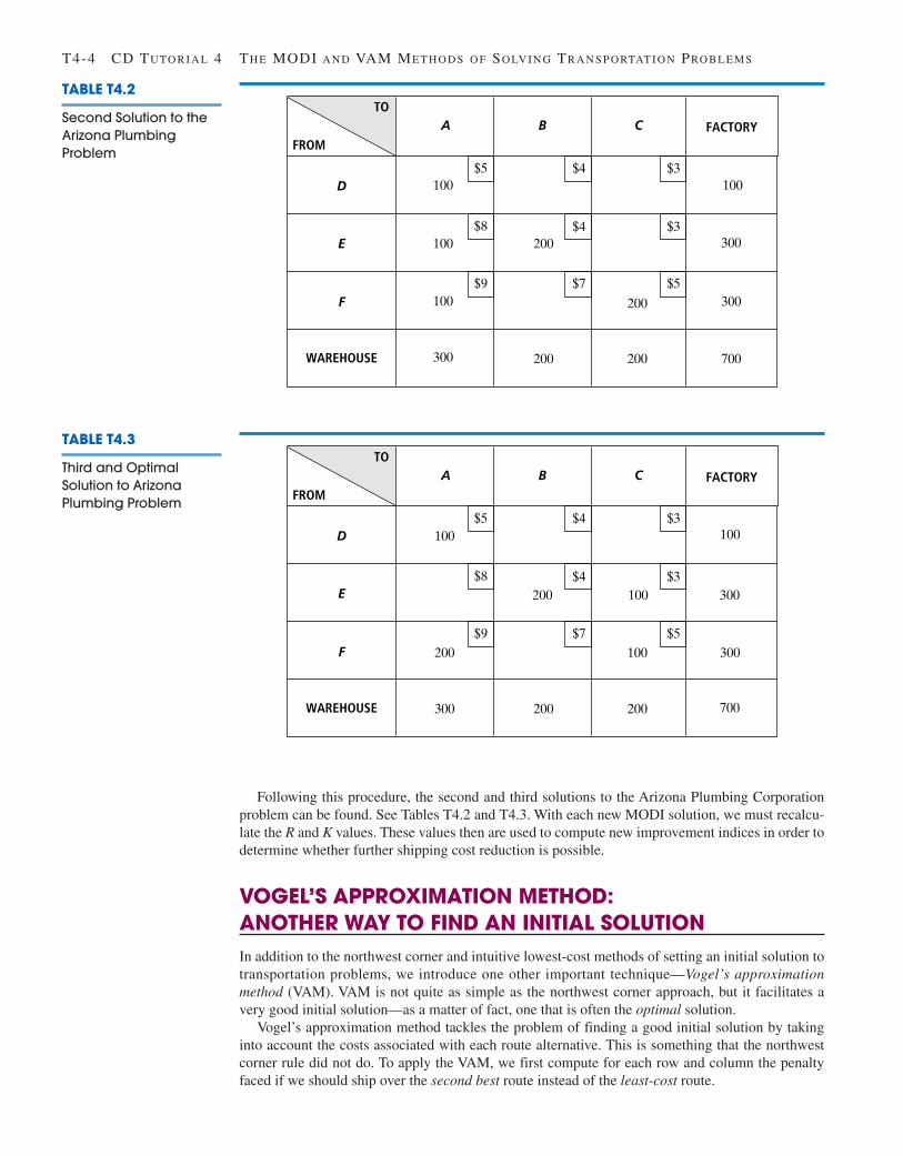
Following this procedure, the second and third solutions to the Arizona Plumbing Corporationproblem can be found. See Tables T4.2 and T4.3. With each new MODI solution, we must recalcu-late the R and K values. These values then are used to compute new improvement indices in order todetermine whether further shipping cost reduction is possible.

VOGEL’S APPROXIMATION METHOD: ANOTHER WAY TO FIND AN INITIAL SOLUTIONIn addition to the northwest corner and intuitive lowest-cost methods of setting an initial solution totransportation problems, we introduce one other important technique—Vogel’s approximationmethod (VAM). VAM is not quite as simple as the northwest corner approach, but it facilitates avery good initial solution—as a matter of fact, one that is often the optimal solution.

Vogel’s approximation method tackles the problem of finding a good initial solution by takinginto account the costs associated with each route alternative. This is something that the northwestcorner rule did not do. To apply the VAM, we first compute for each row and column the penaltyfaced if we should ship over the second best route instead of the least-cost route.

VO G E L’S AP P ROX I M AT I O N ME T H O D: AN OT H E R WAY TO FI N D A N IN I T I A L SO L U T I O N T4-5

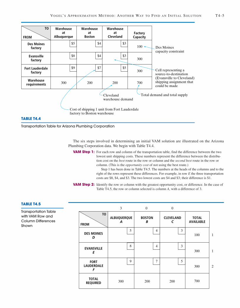
The six steps involved in determining an initial VAM solution are illustrated on the ArizonaPlumbing Corporation data. We begin with Table T4.4.

VAM Step 1: For each row and column of the transportation table, find the difference between the twolowest unit shipping costs. These numbers represent the difference between the distribu-tion cost on the best route in the row or column and the second best route in the row orcolumn. (This is the opportunity cost of not using the best route.)

Step 1 has been done in Table T4.5. The numbers at the heads of the columns and to theright of the rows represent these differences. For example, in row E the three transportationcosts are $8, $4, and $3. The two lowest costs are $4 and $3; their difference is $1.

VAM Step 2: Identify the row or column with the greatest opportunity cost, or difference. In the case ofTable T4.5, the row or column selected is column A, with a difference of 3.

TABLE T4.4

Transportation Table for Arizona Plumbing Corporation

FROM

TO

Des Moinesfactory

Warehouseat

Albuquerque

Warehouseat

Boston

Warehouseat

ClevelandFactoryCapacity

Evansvillefactory

Fort Lauderdalefactory

Warehouserequirements

$5 $4 $3100

$8

Cost of shipping 1 unit from Fort Lauderdalefactory to Boston warehouse

Clevelandwarehouse demand

Total demand and total supply

Cell representing asource-to-destination(Evansville to Cleveland)shipping assignment thatcould be made

Des Moinescapacity constraint

$4 $3300

$9 $7 $5300

700200200300

TABLE T4.5

Transportation Tablewith VAM Row andColumn DifferencesShown FROM

TOALBUQUERQUE

ABOSTON

BCLEVELAND

CTOTAL

AVAILABLE

DES MOINESD

EVANSVILLEE

FORTLAUDERDALE

F

TOTALREQUIRED

5

8

3 0 0

4 3

300

300

100

2

1

1

4 3

9 7 5

700200300 200

T4-6 CD TU TO R I A L 4 TH E MODI A N D VAM ME T H O D S O F SO LV I N G TR A N S P O RTAT I O N PRO B L E M S

TABLE T4.6

VAM Assignment with D’sRequirements Satisfied

FROM

TO

A B C TOTALAVAILABLE

D

E

F

TOTALREQUIRED

5

8

4 3

300

300

100

4 3

9 7 5

700200300

100 X X

200

2

1

1

3 1 0 3 0 2

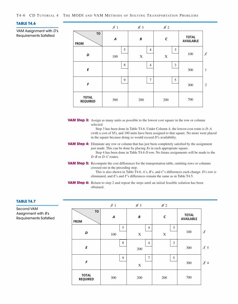
VAM Step 3: Assign as many units as possible to the lowest cost square in the row or columnselected.

Step 3 has been done in Table T4.6. Under Column A, the lowest-cost route is D–A(with a cost of $5), and 100 units have been assigned to that square. No more were placedin the square because doing so would exceed D’s availability.

VAM Step 4: Eliminate any row or column that has just been completely satisfied by the assignmentjust made. This can be done by placing Xs in each appropriate square.

Step 4 has been done in Table T4.6 D row. No future assignments will be made to theD–B or D–C routes.

VAM Step 5: Recompute the cost differences for the transportation table, omitting rows or columnscrossed out in the preceding step.

This is also shown in Table T4.6. A’s, B’s, and C’s differences each change. D’s row iseliminated, and E’s and F’s differences remain the same as in Table T4.5.

VAM Step 6: Return to step 2 and repeat the steps until an initial feasible solution has beenobtained.

TABLE T4.7

Second VAMAssignment with B’sRequirements Satisfied

FROM

TO

A B C TOTALAVAILABLE

D

E

F

TOTALREQUIRED

5

8

3 1 0 3 0 2

4 3

300

300

100

2 4

1 5

1

4 3

9 7 5

700200

200

300

100 X

X

X

200

VO G E L’S AP P ROX I M AT I O N ME T H O D: AN OT H E R WAY TO FI N D A N IN I T I A L SO L U T I O N T4-7

TABLE T4.8

Third VAM Assignmentwith C’s RequirementsSatisfied FROM

TO

A B C TOTALAVAILABLE

D

E

F

TOTALREQUIRED

5

8

4 3

300

300

100

4 3

9 7 5

700200

200 100X

300

100 X

X

X

200

In our case, column B now has the greatest difference, which is 3. We assign 200 units to the low-est-cost square in column B that has not been crossed out. This is seen to be E–B. Since B’s require-ments have now been met, we place an X in the F–B square to eliminate it. Differences are onceagain recomputed. This process is summarized in Table T4.7.

The greatest difference is now in row E. Hence, we shall assign as many units as possible to thelowest-cost square in row E, that is, E–C with a cost of $3. The maximum assignment of 100 unitsdepletes the remaining availability at E. The square E–A may therefore be crossed out. This is illus-trated in Table T4.8.

The final two allocations, at F–A and F–C, may be made by inspecting supply restrictions (in therows) and demand requirements (in the columns). We see that an assignment of 200 units to F–Aand 100 units to F–C completes the table (see Table T4.9).

The cost of this VAM assignment is = (100 units × $5) + (200 units × $4) + (100 units × $3) +(200 units × $9) + (100 units × $5) = $3,900.

It is worth noting that the use of Vogel’s approximation method on the Arizona PlumbingCorporation data produces the optimal solution to this problem. Even though VAM takes manymore calculations to find an initial solution than does the northwest corner rule, it almost alwaysproduces a much better initial solution. Hence VAM tends to minimize the total number of compu-tations needed to reach an optimal solution.

TABLE T4.9

Final Assignments toBalance Column andRow Requirements FROM

TO

A B C TOTALAVAILABLE

D

E

F

TOTALREQUIRED

5

8

4 3

300

300

100

4 3

9 7 5

700200

200 100X

300

100

200 100

X

X

X

200

�T4-8 CD TU TO R I A L 4 TH E MODI A N D VAM ME T H O D S O F SO LV I N G TR A N S P O RTAT I O N PRO B L E M S

DISCUSSION QUESTIONS

P:

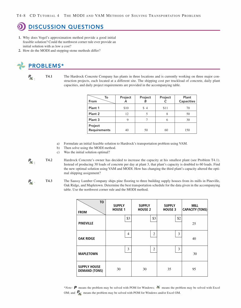
To Project Project Project PlantFrom A B C Capacities

Plant 1 $10 $ 4 $11 70

Plant 2 12 5 8 50

Plant 3 9 7 6 30

Project Requirements 40 50 60 150

P�

P .

FROM

TOSUPPLYHOUSE 1

SUPPLYHOUSE 2

SUPPLYHOUSE 3

MILLCAPACITY (TONS)

PINEVILLE

OAK RIDGE

MAPLETOWN

SUPPLY HOUSEDEMAND (TONS)

$3

25

4

$3 $2

2 3

3 2 3

3030 35

40

30

95

1. Why does Vogel’s approximation method provide a good initialfeasible solution? Could the northwest corner rule ever provide aninitial solution with as low a cost?

2. How do the MODI and stepping-stone methods differ?

PROBLEMS*

T4.1 The Hardrock Concrete Company has plants in three locations and is currently working on three major con-struction projects, each located at a different site. The shipping cost per truckload of concrete, daily plantcapacities, and daily project requirements are provided in the accompanying table.

a) Formulate an initial feasible solution to Hardrock’s transportation problem using VAM.b) Then solve using the MODI method.c) Was the initial solution optimal?

T4.2 Hardrock Concrete’s owner has decided to increase the capacity at his smallest plant (see Problem T4.1).Instead of producing 30 loads of concrete per day at plant 3, that plant’s capacity is doubled to 60 loads. Findthe new optimal solution using VAM and MODI. How has changing the third plant’s capacity altered the opti-mal shipping assignment?

T4.3 The Saussy Lumber Company ships pine flooring to three building supply houses from its mills in Pineville,Oak Ridge, and Mapletown. Determine the best transportation schedule for the data given in the accompanyingtable. Use the northwest corner rule and the MODI method.

*Note: means the problem may be solved with POM for Windows; means the problem may be solved with Excel

OM; and means the problem may be solved with POM for Windows and/or Excel OM.P

P:

PRO B L E M S T4-9

P:

T4.4 The Krampf Lines Railway Company specializes in coal handling. On Friday, April 13, Krampf had empty carsat the following towns in the quantities indicated:

Town Supply of Cars

Morgantown 35Youngstown 60Pittsburgh 25

By Monday, April 16, the following towns will need coal cars:

Town Demand for Cars

Coal Valley 30Coaltown 45Coal Junction 25Coalsburg 20

Using a railway city-to-city distance chart, the dispatcher constructs a mileage table for the preceding towns.The result is

To

From Coal Valley Coaltown Coal Junction Coalsburg

Morgantown 50 30 60 70Youngstown 20 80 10 90Pittsburgh 100 40 80 30

Minimizing total miles over which cars are moved to new locations, compute the best shipment of coal cars.Use the northwest corner rule and the MODI method.

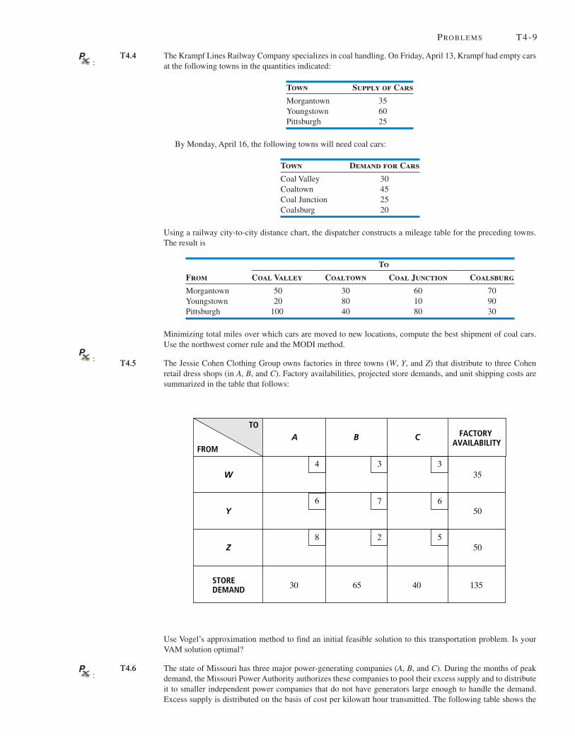
T4.5 The Jessie Cohen Clothing Group owns factories in three towns (W, Y, and Z) that distribute to three Cohenretail dress shops (in A, B, and C). Factory availabilities, projected store demands, and unit shipping costs aresummarized in the table that follows:

Use Vogel’s approximation method to find an initial feasible solution to this transportation problem. Is yourVAM solution optimal?

T4.6 The state of Missouri has three major power-generating companies (A, B, and C). During the months of peakdemand, the Missouri Power Authority authorizes these companies to pool their excess supply and to distributeit to smaller independent power companies that do not have generators large enough to handle the demand.Excess supply is distributed on the basis of cost per kilowatt hour transmitted. The following table shows the

P:

FROM

TOA B C FACTORY

AVAILABILITY

W

Y

Z

STOREDEMAND

435

50

50

6

3 3

7 6

8 2 5

6530 40 135

T4-10 CD TU TO R I A L 4 TH E MODI A N D VAM ME T H O D S O F SO LV I N G TR A N S P O RTAT I O N PRO B L E M S

To W X Y Z ExcessFrom Supply

A 12¢ 4¢ 9¢ 5¢ 55

B 8¢ 1¢ 6¢ 6¢ 45

C 1¢ 12¢ 4¢ 7¢ 30

Unfilled Power Demand 40 20 50 20

Use Vogel’s approximation method to find an initial transmission assignment of the excess power supply. Thenapply the MODI technique to find the least-cost distribution system.

demand and supply in millions of kilowatt hours and the costs per kilowatt hour of transmitting electric powerto four small companies in cities W, X, Y, and Z.