The Meteorology of Tornado Forecasting:Basic Concepts

Rich ThompsonSPC

Rich

Roger

Shut up!I wanna play the

dryline!

STPs arehigh along the warm

front

• Grew up in Houston, TX, with a life-long interest in weather

• Meteorology graduate from OU• Worked at NWSFO Houston 1992-94• Been with SELS/SPC since July 1994• Lead Forecaster with SPC since 2000• Storm chasing experience since 1985

Who am I?

Why am I here?

• Simple goal – I want to share what I’ve learned over the course of my career, before I forget everything!

• Want to help people make better forecasts for severe thunderstorms:– Appreciation for what goes into SPC forecasts– Link meteorological concepts to aspects of course work

and operational meteorology– Better storm chasing strategies

Workshop Organization

1. Observations, convective processes, and synoptic processes:

How to read weather maps and sounding diagrams “Q-G Theory”, jet streaks, fronts, cyclones

2. Severe thunderstorm ingredients: Moisture and lapse rate sources

3. Severe thunderstorm ingredients: Lift and vertical wind shear sources

4. Supercell and tornado conceptual models Reasons behind parameter development

Workshop Organization Cont’d

5. Synoptic tornado patterns 6. Convective mode 7. Tornado parameter climatology 8. Numerical models and statistical approaches 9. Forecasting exercise

Map Plots of Observed Data

• Station model plots• Contour analysis• General rules to follow with contours for

various fields– T, Td, height, wind

Surface Station Model

Wind Direction and Speed

Upper Air Station Model

Height (m above sea level)of pressure level

Temperature (C) at pressure level

Dew point (C) at pressure level

Wind direction (from) and speed (knots)

Rules for Contour Analysis

• Surface plots:– Temperature (T) limits the dew point temperature (Td)– Wind speed related to spacing of pressure contours

(pressure gradient), but wind usually crosses toward lower pressure due to friction near the ground

• Upper air plots:– Same limitations as surface with T and Td– Wind largely parallel to “geopotential height” contours– Geopotential height ≈ height above sea level of a pressure

surface

Raw SkewT-log P diagram

Constant Temp

Dry adiabat

“skew”

Constant pressure

ConstantMixing ratio

Features of note in SkewT log P

• Temperature is skewed about 90o from the dry adiabats

• Pressure decreases as a logarithm of height (faster at bottom than top)

• Mixing ratio crosses over temperature lines– It’s a function of pressure, which is why the same dew point

temperature at higher elevation contributes more to buoyancy

• One thing missing is a plot of saturated parcel ascent

Dry ascent (no clouds) –parcel cools at a rate of ~9.8 C km-1

(dry adiabatic “lapse rate”)

Saturated ascent (clouds) –parcel cools at a rate of~6.5 C km-1

(pseudo adiabatic “lapse rate”)

Lapse rates between saturated and unsaturated – “conditionally unstable”

Lifted Parcel (chunk of air)

• Begin at lifted parcel level (ground)• Rise “dry adiabatically” until saturation

– Where dry adiabat crosses mixing ratio– We call this the “lifting condensation level” or LCL– First guess at cloud base

Moist adiabat

Illustration of lifted parcel

• From LCL, rise “moist adiabatically” to “level of free convection” or LFC– “Free convection” begins where lifted parcel becomes

warmer than environment– Energy resisting lift below LFC is known as “convective

inhibition” or CIN

• From LFC, continue up to the “equilibrium level” or EL. Accumulated area (energy) from LFC to EL is known as CAPE– “Overshoot” above EL

Common Sounding Terms

• Lapse rate – change in temperature with height – Dry adiabat ≈ 9.8 C km-1

– Moist adiabat ≈ 6.5 C km-1 • Conditional instability – lapse rate between dry and

moist adiabatic• LCL – lifting condensation level• LFC – level of free convection• EL – equilibrium level• CAPE – buoyancy (positive area)• CIN – convective inhibition (negative area)

Positive area (CAPE)

Negative area (CIN)

What’s the difference between the lifted parcels?

• Virtual temperature accounts for moisture – Warmer than measured temperature– Makes most difference with tropical moisture

• Virtual temperature correction increases CAPE and reduces CIN

• Which chunk of air to lift?– Some sort of averaging is usually more representative– Surface vs. “mixed layer” or “most unstable”

Lifted parcel (virtual temp)

Lifted parcel(non-virtual)

Surface and most unstable parcel are the same

Lowest 100 mb mean parcel

Surface parcel

100 mb mean parcel

Most unstable parcel

What are we assuming?

• No mixing with environment (not true)– “entrainment” usually reduces updraft strength from

expectations based on CAPE alone

• All rain falls out instantly (not true)– Suspended rain particles reduces updraft strength– That’s why we say “pseudo” adiabatic for saturated parcel

ascent

• “Parcel Theory” is a first guess at a complicated process!

Always keep in mind what we don’t know:

• Uncertainty in observations– “Good” measurements?– Do they represent what we’re trying to forecast?

• Unknown details with lifted parcels– What is right layer to view?– What assumptions are valid, and which might be terribly

wrong?

• Lots of room for error, but the concepts are useful!

Simple vertical mixing

• Surface heating drives thermals and mixing, which take heat and moisture both upward (from surface) and downward (from aloft)

• Usually see surface dew point drop in afternoon if not offset by moisture advection (bringing in greater moisture from somewhere else)

Surface heating drives vertical mixing

“super adiabatic” contact layer – lapse rate steeper than dry adiabatic drives vertical mixing

Impact of ascent and moisture advection

• See moist layer deepen faster than you would expect with just surface heating and mixing

• “Deep” moist layer and horizontal moisture advection both combat vertical mixing driven by surface heating– Can see moist layer deepen while dew points increase

near surface

Hodograph and Vertical Wind Shear

• Hodograph is the trace connecting the ends of wind vectors with height– Shows change in wind speed/direction with height on a

simple plot

• Vertical wind shear can be calculated from the hodograph– Vector wind differences and storm-relative winds

Plot tips of vectors with height

SFC

1 km

2 km

Wind Shear from Hodograph

Shear vector SFC to 2 km

Shear vector 1 km to 9 km

Storm-relative Winds

Surface storm-relative wind vector

Storm motion

Horizontal vorticity vectors –perpendicular to hodograph

Storm-relative Winds

Storm-relative helicity – area “swept out” between storm motion and hodograph

Sounding diagrams are used for…

• Moisture and temperature profiles• Estimates of CAPE, CIN, Lifted Index, etc.

– Will storms form?

• Vertical wind shear– What kind of storms will form?

• Many of your favorite thunderstorm parameters are based in these diagrams, and subject to the same errors and concerns!

Synoptic Meteorology

• Need to understand what “weather maps” show

• Need to understand how different processes are related– Fronts and cyclogenesis– “Q-G Theory” and vertical motion

• First, make sure you understand the data plots and sources for errors!

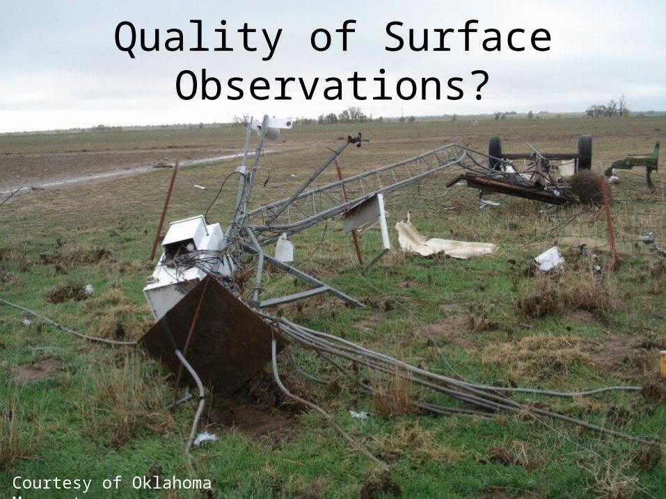
Quality of Surface Observations?

Courtesy of Oklahoma Mesonet

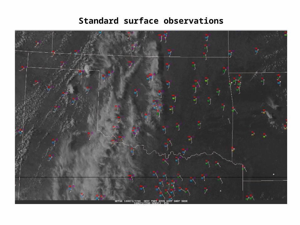
Standard surface observations

OK mesonet observations at the same time

Dew point analysis for OK mesonet observations

What do these sites have in common?

68

73

6863

Quality of Observations Aloft?

Understand the Data and Processes!

• Understanding the processes gives you a sound way to interpret weather data, and recognize errors

• If you don’t know what you’re using, how do you know if you’re using it correctly?– Must consider data quality

• Focus on observations!

The Meteorology of Tornado Forecasting:Synoptic Meteorology

Rich ThompsonSPC

Concepts in Synoptic Meteorology

• Synoptic pattern evolution:– System movement and intensity– Contributions to vertical motion and vertical wind shear

• Q-G Theory• Fronts and Jet Streaks• Vertical motion is atmosphere’s attempt to

restore “hydrostatic” and “geostrophic” balance!

Geostrophic Wind

• Pressure gradient and Coriolis forces in balance– Winds parallel to height contours aloft– Wind speeds proportional to contour spacing

• Vertical motion is the result of ageostrophic flow and imbalances in the atmosphere

• Real atmosphere more closely resembles gradient wind balance

Gradient Wind Balance

• Curvature in flow changes the balance of forces, adding centrifugal accelerations

• Flow in a trough is subgeostrophic– Results in divergence downstream from trough

• Flow in a ridge is supergeostrophic– Results in convergence downstream from ridge

Gradient Wind < Geostrophic Wind within a low/trough

Gradient Wind > Geostrophic Wind within a ridge/high

Fastest flow in ridge

Slowest flow in trough

Example

Mass Continuity

• Divergence increasing with height – same as convergence decreasing with height

Thickness and Thermal Advection

• Warming in layer results in expansion– Thickness increases around level of max warming– Density of column decreases– Height rises above, height falls below

• Cooling in a layer results in contraction– Thickness decreases around level of max cooling– Density of column increases– Height falls above, height rises below

Atmospheric Thickness

Max warming

Layer expands – thickness increases

Atmospheric Thickness

Max cooling

Layer shrinks – thickness decreases

Thermal Wind

• Not a real wind– Relationship between temperature gradient and the

change in geostrophic winds with height– Veering with height warm advection– Backing with height cold advection

• Winds increase with height above a strong temperature gradient– Jet streams/streaks associated with enhanced belts of

~horizontal temperature gradient

Edge of stronger gradient near ground

Temp gradient slopes NW with height

“Vorticity” and “Advection”

• Vorticity = tendency for “spin”– Think of paddle wheel example

• Advection = transport of an atmospheric quantity– Wind bringing air with different temperature,

moisture, or vorticity to a location

Advection Example

CVA

AVA

Quasi-Geostrophic (Q-G) Theory

• Assume mostly geostrophic flow• Only consider advection by the geostrophic

wind • Ageostrophic flow allowed as part of the

response to Q-G forcing– Very simple version of real atmosphere

Q-G Height Tendency Equation

• Height change = Term 1 + Term 2• Term 1 = geostrophic vorticity advection by the

geostrophic wind– Referred to as vorticity advection (CVA or AVA)– CVA leads to height falls

• Term 2 = Differential geostrophic thickness advection– Referred to as differential thermal advection– Height rises above level of max warm advection– Same idea as thickness change (hypsometric equation)

Q-G Height Tendency

• Height falls with CVA• Max in thermal advection

– Warm advection max leads to height falls below and height rises above

• Surface pressure falls with thickness increase above

– Cold advection max leads to height falls above and height rises below

• Surface pressure rises with thickness decrease above

Q-G “Omega” Equation

• Vertical motion = Term 1 + Term 2• Term 1 = differential advection of absolute

geostrophic vorticity by the geostrophic wind– Referred to a differential vorticity advection

• Term 2 = thermal advection• Both terms scaled by static stability

– Stronger response with steeper lapse rates

Q-G Vertical Motion

• Differential cyclonic vorticity advection (CVA)– Rising motion where CVA increases with height

• CVA increasing with height = divergence increasing with height, which is the same as ascent through mass continuity

– Sinking motion where CVA decreases with height

• Thermal advection– Rising motion with warm advection– Sinking motion with cold advection– Easy to see with “isentropic” charts

Frontogenesis

• Strengthening of temperature gradient:– Response of atmosphere is to weaken gradient

• Ascent on warm side of front (cooling)• Descent on cool side of front (warming)

• Fronts are zones where thermal advection is easily enhanced, and fronts are often preferred corridors for cyclogenesis– Cyclones tend to move along existing fronts

Jet Streaks with Straight Flow

• Explain patterns of rising and sinking motion• Divide jet streak into regions

– Entrance (upstream) and exit (downstream) regions– Left and right side of each region

• Use two physical explanations – Q-G vertical motion equation– Frontogenesis– Both give same answer, which is good!

Q-G Vorticity Explanation

AVA

AVA

CVA

CVA

Jet Streaks and Q-G Theory

• Cyclonic and anticyclonic vorticity (spin) is created on sides of jet streak

• From Q-G approach, differential CVA is the same as differential divergence = ascent

• The simple graphic only shows CVA at one level – assumes increasing with height below level of strongest jet

Frontogenesis Explanation

Air entering jet streak – sinking on cold side, rising on warm side.

Air leaving jet streak – rising on cold side, sinking on warm side.

Jet Streaks and Frontogenesis

• Jet streaks are coincident with stronger temperature gradients

• Air moving through a jet streak:– Encounters strengthening gradient entrance region– Encounters weakening gradient exit region

• Response to frontogenesis:– Weaken gradient through sinking in cold air and rising in

warm air (entrance region)– Opposite is true in exit region

Jet Streaks and Curved Flow

• Curved flow much more common• Change from 4 regions (quadrants) to 2

regions as result of along-stream ageostrophic flow (recall gradient wind balance):– Ascent focused close to jet axis, with ascent extending into

right exit region for cyclonically curved jet– Ascent tends to be stronger than with a straight jet streak

because more atmospheric adjustment necessary to restore balance

“Baroclinic” Systems

• Temperature advection and system tilt with height (upstream):– Often deepening cyclones or rapid movement– Differential advection leads to destabilization

• Warm advection corresponds to veering winds with height (thermal wind):– Large, clockwise-curved hodographs in warm sector

• Jet streaks and fronts:– Strong speed shear aloft with fronts and jet streaks

Edge of stronger gradient near ground

“Equivalent Barotropic”

• Temperature contours parallel to height contours– Little temperature advection– Usually steady or weakening cyclone

• Without large-scale temperature advection, will see little veering of winds with height– Usually weak low-level shear– Unidirectional flow in warm sector– Slow system movement

Tying it all together…

• Can explain why ascent occurs downstream from troughs, along fronts, and in exit regions of jets

• Areas of ascent are strongest where gradients are strongest

• Patterns of ascent contribute to cyclone strength and motion

• All relevant to setting the stage for severe thunderstorms!

CancunVeracruz

Brownsville

Lake CharlesTallahassee

What’s up next?

Helpful Links

• http://www2.mmm.ucar.edu/people/tomjr/files/realtime/qgomega-usersguide.pdf

• https://www.meted.ucar.edu/bom/qgoe/• http://

www.crh.noaa.gov/images/lmk/QG_Theory_Review.pdf

• http://ww2010.atmos.uiuc.edu/%28Gh%29/guides/mtr/fw/grad.rxml