The Message Delay in Mobile Ad Hoc Networkskoole/publications/2005pe/art.pdf · The Message Delay in Mobile Ad Hoc Networks ... the Netherlands. E-mail: [email protected]. 1. Routing

The Message Delay in Mobile Ad Hoc Networks

Robin Groenevelt∗ Philippe Nain∗ Ger Koole††

Abstract

A stochastic model is introduced that accurately models the message delay in mobile ad hoc networks

where nodes relay messages and the networks are sparsely populated. The model has only two input param-

eters: the number of nodes and the parameter of an exponential distribution which described the time until

two random mobiles come with communication range of one another. Closed-form expressions are obtained

for the Laplace-Stieltjes transform of the message delay, defined as the time needed to transfer a message

between a source and a destination. From this result, the first two moments of the expected message delay

are derived in closed-form as well as their asymptotic expansion for large networks. As an additional result,

the probability distribution function is obtained for the number of copies of the message at the time the

message is delivered. These calculations are carried out for two protocols: the two-hop multicopy and the

unrestricted multicopy protocols. It is shown that despite its simplicity, the model accurately predicts the

message delay for both relay strategies for a number of mobility models (the random waypoint, random

direction and the random walker mobility models).

1 Introduction

In mobile ad hoc networks (MANET), a mobile (or simply a node) can only send data to another node if both

nodes are within transmission range of one another or in contact. Two nodes are within transmission range of

one another if the distance between them does not exceed r.

The fact that two nodes are in contact is of course not enough to ensure the success of a transmission, since

many phenomena may occur during the transmission and cause it to fail (interference, physical obstacles, power

problems, etc.). Message relaying is a technique that reduces message latency by using intermediary nodes to

forward the message.∗INRIA, BP 93, 06902 Sophia Antipolis, France. E-mail: {rgroenev, nain}@sophia.inria.fr.†Vrije Universiteit, Boelelaan 1081a, 1081 HV Amsterdam, the Netherlands. E-mail: [email protected].

1

Routing protocols using relay nodes [11, 12, 19] have been proposed that increase the message delivery ratio

in mobile ad hoc networks. These protocols operate on a store-carry-forward mode to take advantage of node

mobility to improve node connectivity, and ultimately the message throughput. When information is available

(node movement, node position, etc.) these protocols may use it in a static [19] or in a dynamic [11] way. The

concept of relay nodes can also be used in the case when no information on the nodes is available [12].

Evaluating the performance of relay protocols (message delivery ratio, message latency, throughput, etc.) is

a difficult task due to the inherent complexity of mobile ad hoc networks, particularly the random nature of

both the movement of the nodes and of the demand (traffic). The performance of mobile ad hoc networks is

in general studied via lengthy and complex simulations, for a limited number of mobility models, including the

random waypoint mobility model [4, 10] or the random direction mobility model [2, 9].

In this paper we introduce a simple stochastic model to evaluate the performance of relay protocols for

MANET. The model is generic and has only two input parameters: the number of nodes in the network and

the intensity (λ) of some identical and independent Poisson processes. In particular, the model does not require

knowledge of the stationary distribution of the location of the nodes as input.

These processes model instances, called meeting times, at which any pair of nodes come within transmission

range of one another. Transmissions between two nodes can only take place at meeting times and are assumed

to be instantaneous. The latter assumption models the situation where the transmission time of a message is

very small with respect to the time needed for two nodes to meet. Therefore, the random nature of a MANET

is captured in our model through a finite number of these independent and homogeneous Poisson processes.

The selection of the intensity λ will be discussed in Sections 3 and 4.

The model is used to characterize the message delay between two arbitrary nodes—hereafter called the

source node and the destination node—for two relay protocols and for three mobility models.

The two relay protocols are the two-hop multicopy and the unrestricted multicopy protocol.

In the two-hop multicopy protocol the source node copies the message to all the nodes it meets along its

route, including of course the destination node. Any node which has received a duplicate copy of the message

from the source node may only forward it to the destination node. Note that this is different from the two-hop

relay protocol proposed in [8]: there a packet is relayed to another node (instead of being copied).

In the unrestricted multicopy protocol the source node copies the message to all the nodes it meets (as in

the two-hop multicopy protocol), but in this protocol any node that carries the message may in turn copy the

message to all the nodes it encounters, along its trajectory.

The three mobility models that we will consider in this paper are the random waypoint, the random direction,

2

and the two-dimensional random walker mobility model. All three models and their mathematical properties

will be described in Section 3.1.

The characterization of the message delay in MANET has received some attention, although explicit expres-

sions are seldomly obtained for two-dimensional mobility models. In [16] it is shown that, under the two-hop

relay protocol, the expected message delay is of the order nTp(n) for the random waypoint mobility model on a

sphere (where n is the number of nodes per unit area and Tp(n) is the transmission time of a message). With

nodes moving as independent Brownian motions on a sphere, it is shown in [17] that the expected message delay

is of the order log2(n)/σ2, where σ2 is the variance parameter of the Brownian motion. In [7] the expected

message delay under the unrestricted multicopy protocol is computed for a unidimensional network topology,

where the nodes move in adjacent segments according to independent and reflected Brownian motions.

The paper is organized as follows: the stochastic model is introduced in Section 2.1, then we compute in

Section 2.2 the Laplace-Stieltjes Transform (LST) of the message delay (Proposition 1). In this proposition,

we also obtain the distribution of the number of copies of the message at the time the message is delivered to

the destination node. In Proposition 2 we calculate the expected message delay in closed-form and also find an

asymptotic for a large number of nodes. These calculations are done for the two relay protocols.

In Section 3, the expected message delay and the distribution of the number of copies of the message found

in Section 2 are compared to results obtained by simulations. The simulations have been carried out for each

of the six combinations of the two relay protocols and the three mobility models. The simulation results are

very close to the analytical results. We observed discrepancies only when the node transmission range is large

with respect to the size of the area in which the nodes move. In addition, an explicit expression is given for

the parameter λ for the random waypoint and the random direction mobility models, and it is shown that it

behaves as a linear function of the transmission range.

The model assumptions have been validated in Section 3 in the absence of interferences (a situation that

will typically occur when the communication radius of the nodes is small with respect to the area in which the

nodes move, and the node density is also small). One way to incorporate interferences into our model is to thin

the meeting time sequences: with some (independent) probability p (resp. 1− p) a transmission occurring at a

meeting time will be a success (resp. failure). Due to the fact that a thinned Poisson process is again a Poisson

process, it is enough to replace λ by λp, with p the probability that a communication fails due to interferences.

On the other hand, we may also argue that the communication radius of the nodes must be small enough

so that interferences remain at an acceptable level. It has been shown in [8] that the transmission range of the

nodes should be of the order 1/√

N for the two-hop relay protocol, in order to maintain a constant capacity per

3

node (with N the number of nodes per unit area). In Section 4 it will be shown how our model can be used to

compute the expected message delay for the two relay protocols considered in this paper when the transmission

range is a decreasing function of N .

A word on the notation: given a function g(N), we write f(N) = O(g(N)) if |f(N)/g(N)| is bounded from

above as N →∞ and f(N) = o(g(N)) if f(N)/g(N) → 0 as N →∞.

2 The Stochastic Model

We consider a network with N +1 identical mobile nodes. There is a single message to be delivered by a source

node to a destination node. Intermediary nodes can be used as relay nodes. The goal is to determine the

distribution of the message delay and the distribution of the number of copies of the message at the time the

message is delivered to the destination node.

We first introduce the model (Section 2.1); then we use it in Section 2.2 to evaluate the performance (message

delay, number of copies) of the two-hop multicopy and the unrestricted multicopy protocols.

2.1 Definition of the Model

An analytical model that would carefully take into account the main features of a MANET (transmission range,

mobility pattern, interferences, fading, etc.) would be mathematically intractable. Instead, we propose a model

where the impact of these features are captured through a single parameter (the parameter λ, see below).

Let 0 ≤ ti,j(1) < ti,j(2) < · · · be the successive meeting times between nodes i and j (i 6= j). Define

τi,j(n) := ti,j(n + 1)− ti,j(n), the n-th inter-meeting time between nodes i and j.

Transmissions between two nodes may only take place at meeting times and are assumed to be instantaneous.

The latter assumption corresponds to the situation where the transmission time of a message between two nodes

is negligible with respect to the time it takes the two nodes to meet one another (this is the case when the

transmission radius is small with respect to the size of the area).

We assume that if a transmission takes place between node i and node j (at some meeting time ti,j(n))

then it will be successful. Assume that node i carries the message just before time ti,j(n). Under the two-hop

multicopy protocol node i will transmit (a copy of) the message to node j at time ti,j(n) if i is the source

node or if j is the destination node. Under the unrestricted multicopy protocol node i will always transmit the

message to node j at time ti,j(n) regardless of the identity of node j.

4

Throughout the paper the following assumption will hold for each relay protocol:

(A) the processes {ti,j(n), n ≥ 1}, 1 ≤ i, j ≤ N +1, i 6= j, are mutually independent and homogeneous Poisson

processes with rate1 λ > 0. Equivalently stated, the random variables (rvs) {τi,j(n)}i,j,n are mutually

independent and exponentially distributed with mean 1/λ.

We introduce:

• T2 (resp. TU ), the message delay under the two-hop (resp. unrestricted) multicopy protocol, defined as

the time needed to send the message (or a copy of the message) from the source to the destination;

• N2 ∈ {1, 2, . . . , N} (resp NU ∈ {1, 2, . . . , N}), the number of duplicate copies of the message in the

network (excluding the original message but including the message at the destination node) at the time

the message is delivered to the destination node.

For θ ≥ 0 let

T ?2 (θ) := E[e−θT2 ], T ?

U (θ) := E[e−θTU ]

be the LST of T2 and TU , respectively.

2.2 Performance of relay protocols

Proposition 1 gives, for each relay protocol, the LST of the message delay and the distribution of the number

of copies.

Proposition 1 (LST of message delay)

Under the two-hop multicopy protocol

T ?2 (θ) =

N∑i=1

i(N − 1)!(N −i)!

(λ

λN + θ

)i

(1)

and

P (N2 = i) =i

N i

(N − 1)!(N −i)!

, i = 1, . . . , N. (2)

Under the unrestricted multicopy protocol

T ?U (θ) =

1N

N∑i=1

i∏j=1

λj(N + 1− j)λj(N + 1− j) + θ

(3)

1Without restrictions we can let λ depend on the number of nodes in the network. This is discussed in Section 4.

5

and

P (NU = i) =1N

, i = 1, . . . , N, (4)

that is, the number of copies is uniformly distributed over {1, . . . , N}. �

Proof. For both the two-hop and the unrestricted multicopy protocols the proof is based on modeling the

number of copies in the network as an absorbing finite-state Markov chain. The transition rates of these Markov

chains will differ for each protocol.

For each protocol the Markov chain takes its values in {1, 2, . . . , N + 1}. The Markov chain is in state

i = 1, 2, . . . , N when there are i copies of the message in the network including the original message, and it is

in state N + 1 when the message has been delivered to the destination node. Note that states 1, 2, . . . , N are

transient states and N + 1 is an absorbing state.

We provide a separate proof for (1)-(2) and (3)-(4).

Proof of (1) and (2):

�� 1 2 3

3λ 2λ λ

2λλ 3λ

(Ν−2)λ (Ν−3)λ

(Ν−2)λ

(Ν−1)λN

(Ν−1)λ

N−1N−2

N+1

Νλ

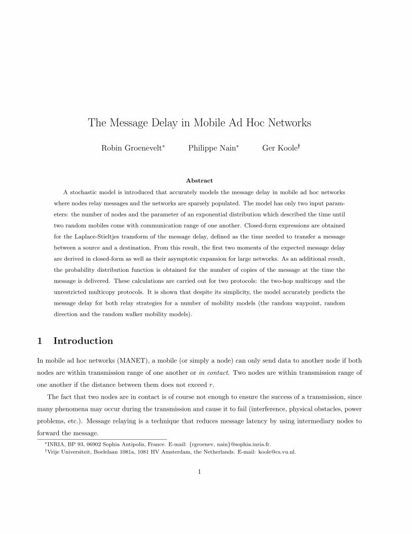
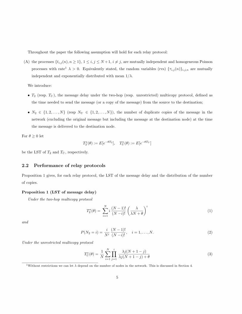
Figure 1: Two-hop multicopy protocol: transition diagram of the Markov chain for the number of copies.

The transition diagram of the Markov chain corresponding to the two-hop multicopy protocol is given in

Figure 1. Recall that under the two-hop multicopy protocol only the source node distributes copies of the

message to nodes that come within its transmission range. Therefore, when there are i copies in the network,

then either a new copy is sent to the N−i nodes which do not have a copy yet, which occurs at the rate λ(N−i)

and triggers a transition from i to i + 1, or one of these i copies reaches the destination node, which occurs at

the rate λi and triggers a transition from i to N + 1. This explains the transition diagram in Figure 1.

The transition from i to N + 1 occurs with the probability iλ/((N − i)λ + iλ) = i/N , and the transition

from i from i + 1 occurs with the complementary probability (N − i))λ/((N − i)λ + iλ) = 1− i/N .

The sojourn time Si in state i = 1, 2, . . . , N is exponentially distributed with intensity λN (the sum of

transition rates out of state i). Moreover S1, . . . , SN are mutually independent random variables.

6

By conditioning on the state of the Markov chain just before its enters state N + 1, or equivalently by

conditioning on the number of duplicate copies N2 just after the message hits its destination, we have

T ?2 (θ) =

N∑i=1

IE[e−θT2 |N2 = i]P (N2 = i) =N∑

i=1

IE[e−θ∑i

j=1 Sj |N2 = i]P (N2 = i). (5)

As mentioned earlier, 1−j/N (resp. j/N) is the probability of jumping from state j to state j +1 (resp. N +1).

Therefore,

P (N2 = i) =i

N

i−1∏j=1

(1− j

N

)=

i

N i

(N − 1)!(N −i)!

, (6)

which establishes (2).

When in state j = 1, 2, . . . , N , the Markov chain can either enter state j + 1 after a time Sj,1 that is

exponentially distributed with intensity (N + 1 − j)λ, or enter state N + 1 after a time Sj,2, independent of

Sj,1, and exponentially distributed with intensity jλ. Observe that Sj = min{Sj,1, Sj,2}. Moreover

P [Sj,1 < x |Sj,1 < Sj,2] =P [Sj,2 < x |Sj,1 > Sj,2] = P (Sj < x) = 1− exp(−λNx) (7)

as a consequence of the exponential distribution. Therefore,

IE[e−θ∑i

j=1 Sj |N2 = i] =IE[e−θ(∑i−1

j=1 Sj,1+Si,2) |Sj,1 < Sj,2, . . . , Si−1,1 < Si−1,2, Si,1 > Si,2] (8)

From (7), (8) and the fact that the rvs {Sj,k}j=1,...,N,k=1,2 are mutually independent, we readily find

IE[e−θ∑i

j=1 Sj |N2 = i] =i∏

j=1

IE[e−θSj ] =(

λN

λN + θ

)i

. (9)

Putting (5), (6) and (9) together yields

T ?2 (θ) =

N∑i=1

i(N − 1)!(N − i)!

(λ

λN + θ

)i

,

which proves (1).

Proof of (3) and (4):

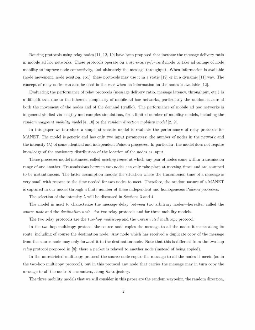
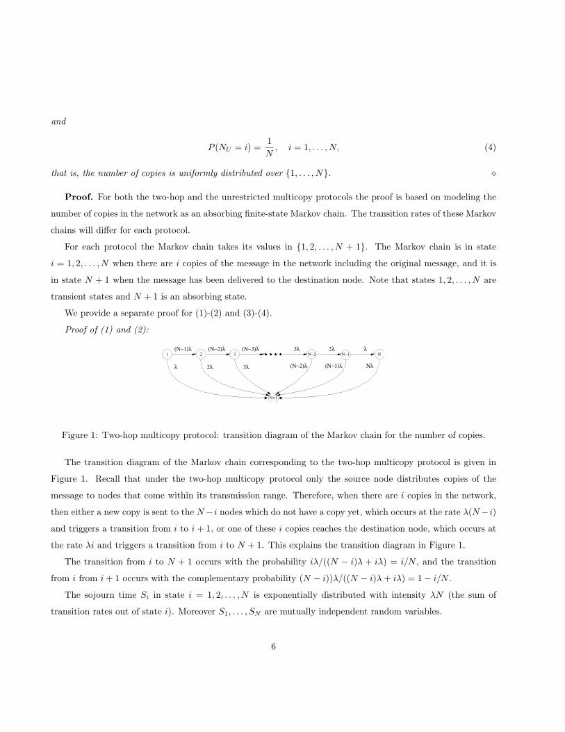
The transition diagram of the Markov chain associated with the unrestricted multicopy protocol is displayed

in Figure 2. Under this protocol, each node which has a copy of the message is allowed to distribute it to a node

which does not have a copy and which comes within its transmission range. Therefore, when there are i copies

of the message in the network a new copy is created at the rate λi(N − i) (transition from i to i+1) and one of

these i copies reaches the destination node at the rate λi (transition from i to N + 1), as depicted on Figure 2.

7

�� 1 2 3

2λλ 3λ

(Ν−1)λ 2(Ν−2)λ 3(Ν−3)λN−2 N

+1N+1

Νλ(Ν−1)λ(Ν−2)λ

N−1(Ν−1)λ(Ν−2)2λ(Ν−3)3λ

Figure 2: Unrestricted multicopy protocol: transition diagram of the Markov chain for the number of copies

The chain jumps from state i to state i + 1 with probability (N − i)/(N + 1− i) and it jumps from state i

to state N + 1 with probability 1/(N + 1− i). The sojourn time Si in state i is exponentially distributed with

intensity λi(N + 1− i) (obtained as the sum of the transition rates going out state i).

By conditioning on the number of duplicate copies NU , we have

T ?U (θ) =

N∑i=1

IE[e−θ∑i

j=1 Sj |NU = i]P (NU = i)

with

P (NU = i) =1

N + 1− i

i−1∏j=1

N − j

N + 1− j=

1N

,

which proves (4).

Similarly to (9) we have

IE[e−θ∑i

j=1 Sj |NU = i] =i∏

j=1

IE[e−θSj ] =i∏

j=1

λj(N + 1− j)λj(N + 1− j) + θ

,

so that

T ?U (θ) =

1N

N∑i=1

i∏j=1

λj(N + 1− j)λj(N + 1− j) + θ

,

which proves (3).

Proposition 2 gives an explicit expression, and an asymptotic for large N , for the expected message delay for

each relay protocol. This result shows that for each protocol the expected message delay is a linear function of

the expected inter-meeting time 1/λ, and changing the value λ does not any impact except for a time scaling.

Proposition 2 (Expected message delays)

Under the two-hop multicopy protocol, the expected message delay is given by

IE[T2] =1

λN

N∑i=1

i2(N − 1)!(N−i)!N i

=1λ

(√π

2N+O

( 1N

)). (10)

8

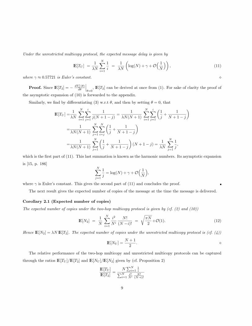
Under the unrestricted multicopy protocol, the expected message delay is given by

IE[TU ] =1

λN

N∑i=1

1i

=1

λN

(log(N) + γ +O

( 1N

)), (11)

where γ ≈ 0.57721 is Euler’s constant. �

Proof. Since IE[T2] = − dT ?2 (θ)dθ

∣∣∣θ=0

, IE[T2] can be derived at once from (1). For sake of clarity the proof of

the asymptotic expansion of (10) is forwarded to the appendix.

Similarly, we find by differentiating (3) w.r.t θ, and then by setting θ = 0, that

IE[TU ] =1

λN

N∑i=1

i∑j=1

1j(N + 1− j)

=1

λN(N + 1)

N∑i=1

i∑j=1

(1j

+1

N + 1− j

)

=1

λN(N + 1)

N∑j=1

N∑i=j

(1j

+1

N + 1− j

)

=1

λN(N + 1)

N∑j=1

(1j

+1

N + 1− j

)(N + 1− j) =

1λN

N∑j=1

1j,

which is the first part of (11). This last summation is known as the harmonic numbers. Its asymptotic expansion

is [15, p. 186]N∑

j=1

1j

= log(N) + γ +O( 1

N

),

where γ is Euler’s constant. This gives the second part of (11) and concludes the proof.

The next result gives the expected number of copies of the message at the time the message is delivered.

Corollary 2.1 (Expected number of copies)

The expected number of copies under the two-hop multicopy protocol is given by (cf. (2) and (10))

IE[N2] =1N

N∑i=1

i2

N i

N !(N −i)!

=

√πN

2+O(1). (12)

Hence IE[N2] = λN IE[T2]. The expected number of copies under the unrestricted multicopy protocol is (cf. (4))

IE[NU ] =N + 1

2. �

The relative performance of the two-hop multicopy and unrestricted multicopy protocols can be captured

through the ratios IE[TU ]/IE[T2] and IE[NU ]/IE[N2] given by (cf. Proposition 2)

IE[TU ]IE[T2]

=N

∑Ni=1

1i∑N

i=1i2

NiN !

(N−i)!

9

and (cf. Corollary 2.1)IE[NU ]IE[N2]

=N(N + 1)

2∑N

i=1i2

NiN !

(N−i)!

,

respectively. Note that both ratios are independent of λ.

By using the asymptotic expansions (10), (11) and (12), we see that

IE[TU ]IE[T2]

≈ log(N)√N

√2π

andIE[NU ]IE[N2]

≈√

N

2π,

for large N . For instance, for N = 103 then IE[TU ]/IE[T2] ≈ 0.17 and IE[NU ]/IE[N2] ≈ 12.6.

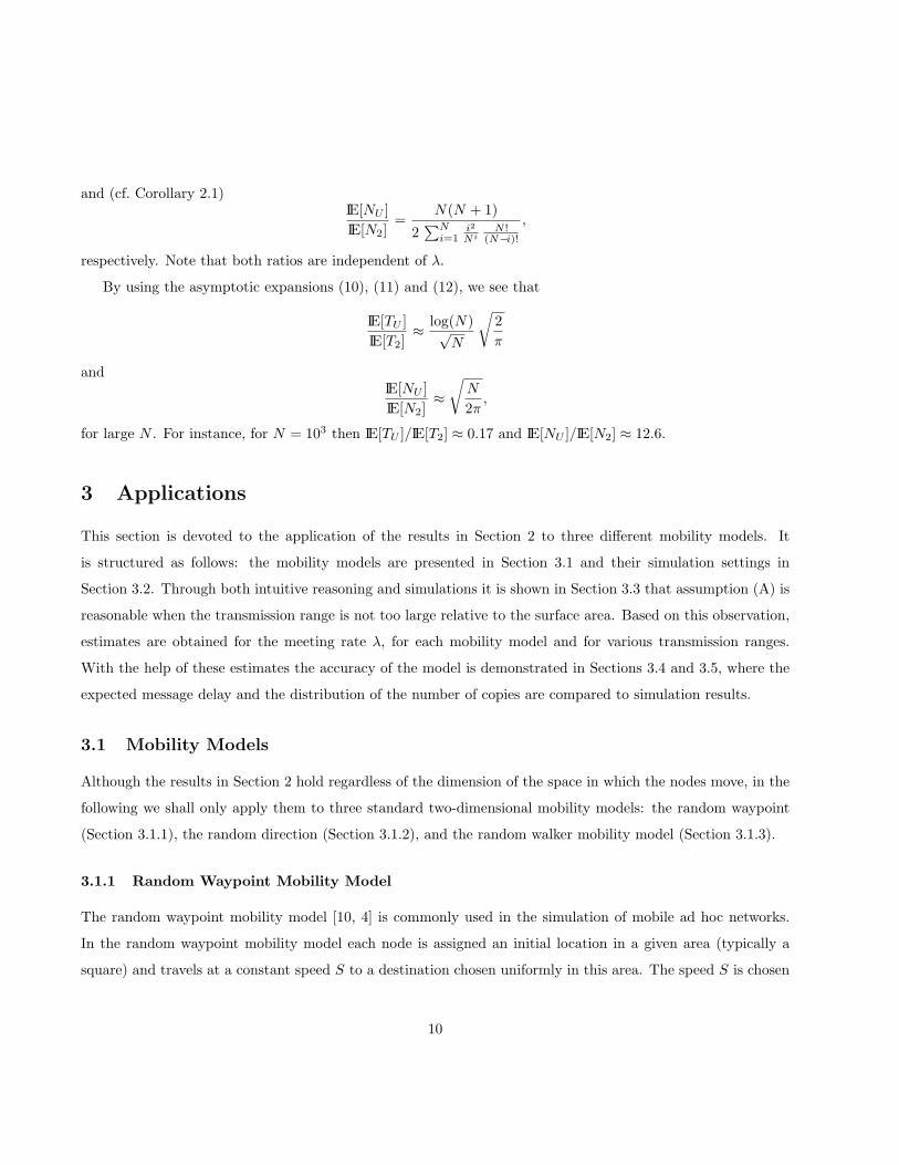
3 Applications

This section is devoted to the application of the results in Section 2 to three different mobility models. It

is structured as follows: the mobility models are presented in Section 3.1 and their simulation settings in

Section 3.2. Through both intuitive reasoning and simulations it is shown in Section 3.3 that assumption (A) is

reasonable when the transmission range is not too large relative to the surface area. Based on this observation,

estimates are obtained for the meeting rate λ, for each mobility model and for various transmission ranges.

With the help of these estimates the accuracy of the model is demonstrated in Sections 3.4 and 3.5, where the

expected message delay and the distribution of the number of copies are compared to simulation results.

3.1 Mobility Models

Although the results in Section 2 hold regardless of the dimension of the space in which the nodes move, in the

following we shall only apply them to three standard two-dimensional mobility models: the random waypoint

(Section 3.1.1), the random direction (Section 3.1.2), and the random walker mobility model (Section 3.1.3).

3.1.1 Random Waypoint Mobility Model

The random waypoint mobility model [10, 4] is commonly used in the simulation of mobile ad hoc networks.

In the random waypoint mobility model each node is assigned an initial location in a given area (typically a

square) and travels at a constant speed S to a destination chosen uniformly in this area. The speed S is chosen

10

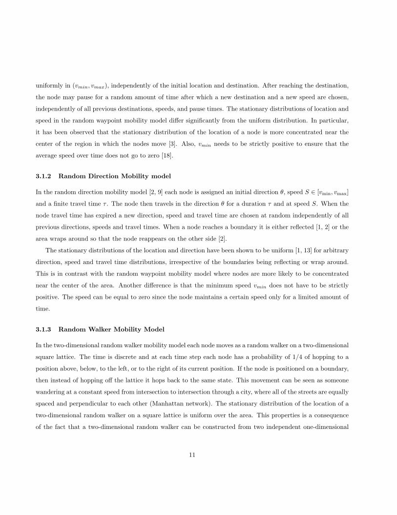
uniformly in (vmin, vmax), independently of the initial location and destination. After reaching the destination,

the node may pause for a random amount of time after which a new destination and a new speed are chosen,

independently of all previous destinations, speeds, and pause times. The stationary distributions of location and

speed in the random waypoint mobility model differ significantly from the uniform distribution. In particular,

it has been observed that the stationary distribution of the location of a node is more concentrated near the

center of the region in which the nodes move [3]. Also, vmin needs to be strictly positive to ensure that the

average speed over time does not go to zero [18].

3.1.2 Random Direction Mobility model

In the random direction mobility model [2, 9] each node is assigned an initial direction θ, speed S ∈ [vmin, vmax]

and a finite travel time τ . The node then travels in the direction θ for a duration τ and at speed S. When the

node travel time has expired a new direction, speed and travel time are chosen at random independently of all

previous directions, speeds and travel times. When a node reaches a boundary it is either reflected [1, 2] or the

area wraps around so that the node reappears on the other side [2].

The stationary distributions of the location and direction have been shown to be uniform [1, 13] for arbitrary

direction, speed and travel time distributions, irrespective of the boundaries being reflecting or wrap around.

This is in contrast with the random waypoint mobility model where nodes are more likely to be concentrated

near the center of the area. Another difference is that the minimum speed vmin does not have to be strictly

positive. The speed can be equal to zero since the node maintains a certain speed only for a limited amount of

time.

3.1.3 Random Walker Mobility Model

In the two-dimensional random walker mobility model each node moves as a random walker on a two-dimensional

square lattice. The time is discrete and at each time step each node has a probability of 1/4 of hopping to a

position above, below, to the left, or to the right of its current position. If the node is positioned on a boundary,

then instead of hopping off the lattice it hops back to the same state. This movement can be seen as someone

wandering at a constant speed from intersection to intersection through a city, where all of the streets are equally

spaced and perpendicular to each other (Manhattan network). The stationary distribution of the location of a

two-dimensional random walker on a square lattice is uniform over the area. This properties is a consequence

of the fact that a two-dimensional random walker can be constructed from two independent one-dimensional

11

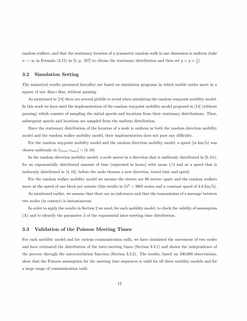
random walkers, and that the stationary location of a symmetric random walk in one dimension is uniform (take

n →∞ in Formula (3.15) in [5, p. 357] to obtain the stationary distribution and then set p = q = 12 ).

3.2 Simulation Setting

The numerical results presented hereafter are based on simulation programs in which mobile nodes move in a

square of size 4km×4km, without pausing.

As mentioned in [14] there are several pitfalls to avoid when simulating the random waypoint mobility model.

In this work we have used the implementation of the random waypoint mobility model proposed in [14] (without

pausing) which consists of sampling the initial speeds and locations from their stationary distributions. Then,

subsequent speeds and locations are sampled from the uniform distribution.

Since the stationary distribution of the location of a node is uniform in both the random direction mobility

model and the random walker mobility model, their implementation does not pose any difficulty.

For the random waypoint mobility model and the random direction mobility model, a speed (in km/h) was

chosen uniformly in [vmin, vmax] = [4, 10].

In the random direction mobility model, a node moves in a direction that is uniformly distributed in [0, 2π),

for an exponentially distributed amount of time (expressed in hours) with mean 1/4 and at a speed that is

uniformly distributed in [4, 10], before the node chooses a new direction, travel time and speed.

For the random walker mobility model we assume the streets are 80 meters apart and the random walkers

move at the speed of one block per minute (this results in 512 = 2601 states and a constant speed of 4.8 km/h).

As mentioned earlier, we assume that there are no inferences and that the transmission of a message between

two nodes (in contact) is instantaneous.

In order to apply the results in Section 2 we need, for each mobility model, to check the validity of assumption

(A) and to identify the parameter λ of the exponential inter-meeting time distribution.

3.3 Validation of the Poisson Meeting Times

For each mobility model and for various communication radii, we have simulated the movement of two nodes

and have estimated the distribution of the inter-meeting times (Section 3.3.1) and shown the independence of

the process through the autocorrelation function (Section 3.3.2). The results, based on 100,000 observations,

show that the Poisson assumption for the meeting time sequences is valid for all three mobility models and for

a large range of communication radii.

12

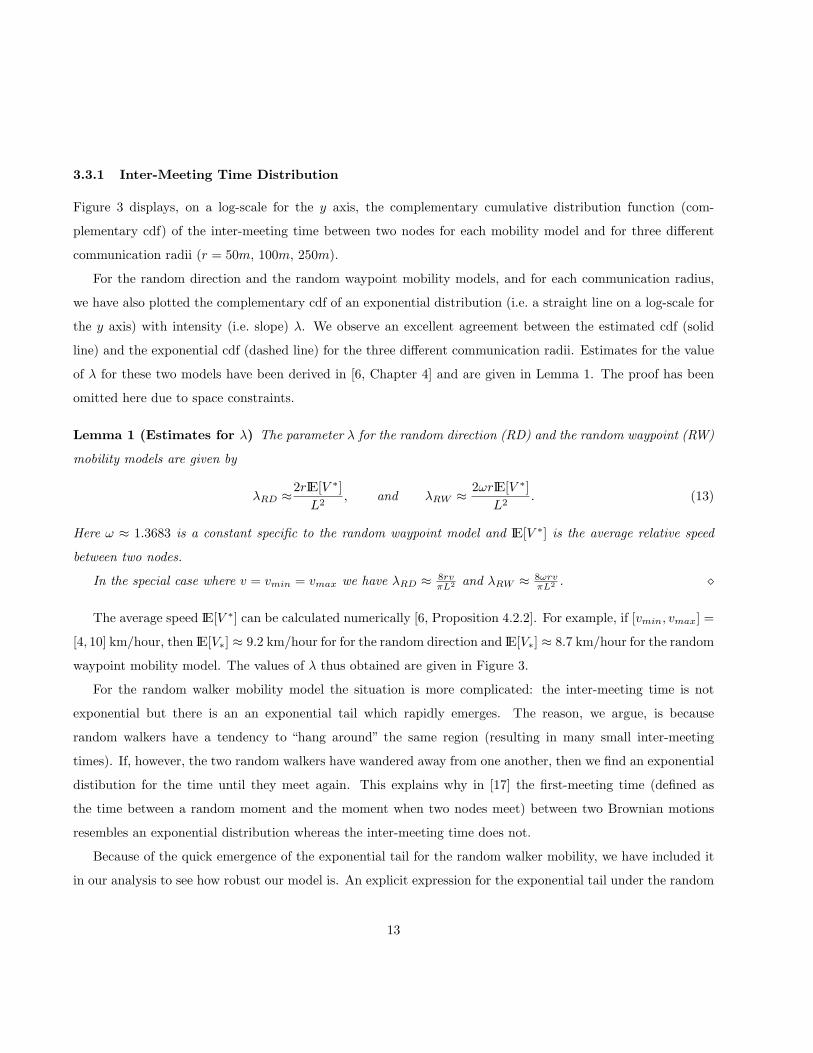
3.3.1 Inter-Meeting Time Distribution

Figure 3 displays, on a log-scale for the y axis, the complementary cumulative distribution function (com-

plementary cdf) of the inter-meeting time between two nodes for each mobility model and for three different

communication radii (r = 50m, 100m, 250m).

For the random direction and the random waypoint mobility models, and for each communication radius,

we have also plotted the complementary cdf of an exponential distribution (i.e. a straight line on a log-scale for

the y axis) with intensity (i.e. slope) λ. We observe an excellent agreement between the estimated cdf (solid

line) and the exponential cdf (dashed line) for the three different communication radii. Estimates for the value

of λ for these two models have been derived in [6, Chapter 4] and are given in Lemma 1. The proof has been

omitted here due to space constraints.

Lemma 1 (Estimates for λ) The parameter λ for the random direction (RD) and the random waypoint (RW)

mobility models are given by

λRD ≈2rIE[V ∗]L2

, and λRW ≈ 2ωrIE[V ∗]L2

. (13)

Here ω ≈ 1.3683 is a constant specific to the random waypoint model and IE[V ∗] is the average relative speed

between two nodes.

In the special case where v = vmin = vmax we have λRD ≈ 8rvπL2 and λRW ≈ 8ωrv

πL2 . �

The average speed IE[V ∗] can be calculated numerically [6, Proposition 4.2.2]. For example, if [vmin, vmax] =

[4, 10] km/hour, then IE[V∗] ≈ 9.2 km/hour for for the random direction and IE[V∗] ≈ 8.7 km/hour for the random

waypoint mobility model. The values of λ thus obtained are given in Figure 3.

For the random walker mobility model the situation is more complicated: the inter-meeting time is not

exponential but there is an an exponential tail which rapidly emerges. The reason, we argue, is because

random walkers have a tendency to “hang around” the same region (resulting in many small inter-meeting

times). If, however, the two random walkers have wandered away from one another, then we find an exponential

distibution for the time until they meet again. This explains why in [17] the first-meeting time (defined as

the time between a random moment and the moment when two nodes meet) between two Brownian motions

resembles an exponential distribution whereas the inter-meeting time does not.

Because of the quick emergence of the exponential tail for the random walker mobility, we have included it

in our analysis to see how robust our model is. An explicit expression for the exponential tail under the random

13

walker mobility model is, to the best of our knowledge, not known and it is therefore obtained numerically as

the complementary of the average first-meeting time obtained across all simulations.

The fact that, for each mobility model, the cdf of the inter-meeting distribution is well-approximated by an

exponential distribution, at least for small to moderate transmission radii (with respect to the size of the area)

finds its roots in the various independence assumptions placed on each mobility model. Indeed, nodes move

independently of each other and future directions and speeds (and therefore locations) of a node are independent

of past directions and speeds of this node. If we pick two mobile nodes at random at some stationary time,

then there is a probability q that they will meet (in the sense of being within transmission range of one another)

before the next change of direction of either node. At the next change of direction, because of the independent

assumptions recalled above, the process repeats itself and there is a probability q that these nodes will meet

before the next change of direction. This yields a geometric distribution for the number of changes of direction

before both nodes meet. The exponential distribution pops up because the number of changes of direction is

“linearly” related to the time traveled before the nodes meet.

0 20 40 60 80 100 12010

−4

10−3

10−2

10−1

100

Random WaypointMobility Model

R=0.05km λ=0.075217

Inter−meeting time (hours)

Com

plem

enta

ry c

df Random WaypointMobility Model

R=0.1km λ=0.14944


R=0.25km λ=0.39248

SimulationExp(λ)

0 20 40 60 80 100 120 140 16010

−4

10−3

10−2

10−1

100

Random DirectionMobility Model

R=0.05km λ=0.057694


Com

plem

enta

ry c

df Random DirectionMobility Model

R=0.1km λ=0.11574


R=0.25km λ=0.29869

SimulationExp(λ)

0 200 400 600 800 1000 120010

−4

10−3

10−2

10−1

100

r=0.05km

r=0.1km

r=0.25km


Com

plem

enta

ry c

df Random walker

Simulation

Figure 3: Complementary cdf of the inter-meeting time of two nodes.

3.3.2 Independence of Inter-Meeting Times

Let {τ(n)}n be the n-th inter-meeting times between two given nodes. To check the assumption that the rvs

{τ(n)}n are mutually independent rvs, we have used the following classical estimator for the autocorrelation

function of {τ(n)}n

ρm(h) =γm(h)γ0(h)

, h ≥ 0,

where

γm(h) :=1m

m−h∑n=1

(τ(n + h)− τ (m)

) (τ(n)− τ (m)

)

14

is an estimator of the autocovariance function, with τ (m) = (1/m)∑m

n=1 τ(n) the sample mean for m observa-

tions. In particular, ρm(h) = 1.

If the rvs {τ(n)}n are mutually independent then their autocorrelation function is equal to zero for all h ≥ 1.

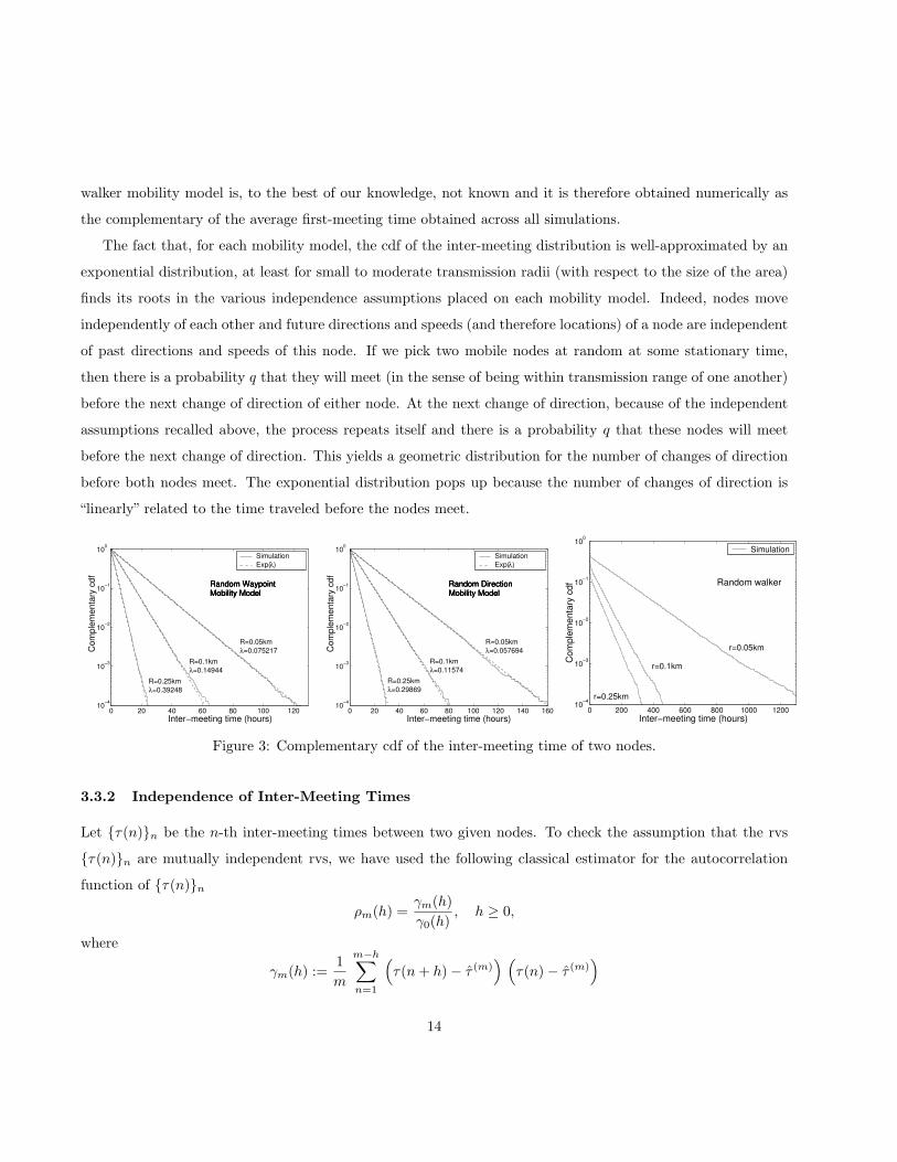
The mapping h → ρm(h) corresponding to the random waypoint mobility model is plotted in Figure 5 for

m = 100, 000 and r = 0.25km. The autocorrelation functions corresponding to other values of r (r = 0.05km,

r = 0.1km) and/or to the random direction mobility model and the random walker mobility model are not

displayed since they are identical to the results in Figure 5.

Since ρm(h) is very close to zero for all h ≥ 1 we conclude that the assumption that the inter-meeting times

between two nodes are mutually independent rvs is a reasonable assumption.

In conclusion, the results reported in Sections 3.3.1 and 3.3.2 validate the assumption that the meeting time

process between two given nodes is a Poisson process for all three mobility models and for small to moderate

communication radii (with respect to the size of the area in which the nodes move).

0 0.05 0.1 0.15 0.2 0.250

0.05

0.1

0.15

0.2

0.25

0.3

0.35

0.4

0.45

Transmission radius (km)

λ

Simulation (random waypoint)λ=1.4817RSimulation (random direction)λ=1.1546R

Figure 4: Relationship between the inter-meeting

time intensity λ and the communication radius r.

0 2 4 6 8 10

0

0.1

0.2

0.3

0.4

0.5

0.6

0.7

0.8

0.9

1

h

Aut

ocor

rela

tion

func

tion

ρ m(h

)

Figure 5: Autocorrelation function of inter-meeting

times for the random waypoint model with r = 0.25km.

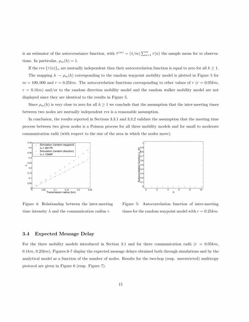
3.4 Expected Message Delay

For the three mobility models introduced in Section 3.1 and for three communication radii (r = 0.05km,

0.1km, 0.25km), Figures 6-7 display the expected message delays obtained both through simulations and by the

analytical model as a function of the number of nodes. Results for the two-hop (resp. unrestricted) multicopy

protocol are given in Figure 6 (resp. Figure 7).

15

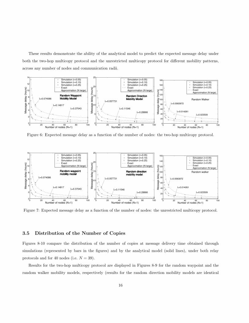
These results demonstrate the ability of the analytical model to predict the expected message delay under

both the two-hop multicopy protocol and the unrestricted multicopy protocol for different mobility patterns,

across any number of nodes and communication radii.

0 20 40 60 80 1000

2

4

6

8

10

12

14

Random WaypointMobility Model λ=0.074086Random WaypointMobility Model

λ=0.14817


λ=0.37043

Number of nodes (N+1)

Mes

sage

del

ay (h

ours

)

Simulation (r=0.05)Simulation (r=0.10)Simulation (r=0.25)ExactApproximation (N large)

0 20 40 60 80 1000

5

10

15

20

25


λ=0.057731


λ=0.11546


λ=0.28866


Mes

sage

del

ay (h

ours

)


0 20 40 60 80 1000

20

40

60

80

100

120

140

160

180

λ=0.0063972

λ=0.014261λ=0.023509


Mes

sage

del

ay (h

ours

)

Random Walker


Figure 6: Expected message delay as a function of the number of nodes: the two-hop multicopy protocol.

0 20 40 60 80 1000

2

4

6

8

10

12

14

Random waypointmobility model

λ=0.074086


λ=0.14817


λ=0.37043


Mes

sage

del

ay (h

ours

)


0 20 40 60 80 1000

5

10

15

20

25

Random directionmobility model

λ=0.057731


λ=0.11546


λ=0.28866


Mes

sage

del

ay (h

ours

)


0 20 40 60 80 1000

20

40

60

80

100

120

140

160

λ=0.0063972

λ=0.014261

λ=0.023509


Mes

sage

del

ay (h

ours

)

Random walker


Figure 7: Expected message delay as a function of the number of nodes: the unrestricted multicopy protocol.

3.5 Distribution of the Number of Copies

Figures 8-10 compare the distribution of the number of copies at message delivery time obtained through

simulations (represented by bars in the figures) and by the analytical model (solid lines), under both relay

protocols and for 40 nodes (i.e. N = 39).

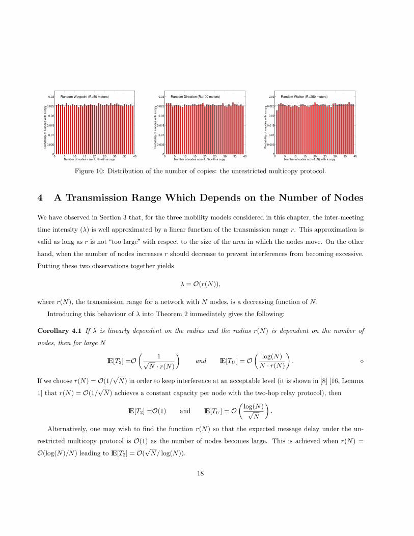
Results for the two-hop multicopy protocol are displayed in Figures 8-9 for the random waypoint and the

random walker mobility models, respectively (results for the random direction mobility models are identical

16

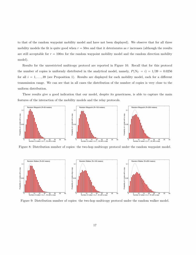
to that of the random waypoint mobility model and have not been displayed). We observe that for all three

mobility models the fit is quite good when r = 50m and that it deteriorates as r increases (although the results

are still acceptable for r = 100m for the random waypoint mobility model and the random direction mobility

model).

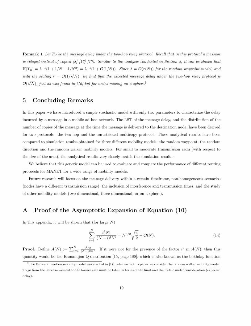
Results for the unrestricted multicopy protocol are reported in Figure 10. Recall that for this protocol

the number of copies is uniformly distributed in the analytical model, namely, P (NU = i) = 1/39 = 0.0256

for all i = 1, . . . , 39 (see Proposition 1). Results are displayed for each mobility model, each for a different

transmission range. We can see that in all cases the distribution of the number of copies is very close to the

uniform distribution.

These results give a good indication that our model, despite its genericness, is able to capture the main

features of the interaction of the mobility models and the relay protocols.

0 5 10 15 20 25 30 35 400

0.05

0.1

Number of nodes n (n=1,..,N) with a copy

Pro

babi

lity

of n

nod

es w

ith a

cop

y

Random Waypoint (R=50 meters)

0 5 10 15 20 25 30 35 400

0.05

0.1


Pro

babi

lity

of n

nod

es w

ith a

cop

y


0 5 10 15 20 25 30 35 400

0.05

0.1


Pro

babi

lity

of n

nod

es w

ith a

cop

y


Figure 8: Distribution number of copies: the two-hop multicopy protocol under the random waypoint model.

0 5 10 15 20 25 30 35 400

0.05

0.1


Pro

babi

lity

of n

nod

es w

ith a

cop

y

Random Walker (R=50 meters)

0 5 10 15 20 25 30 35 400

0.05

0.1

Number of nodes n (n=1..,N) with a copy

Pro

babi

lity

of n

nod

es w

itg a

cop

y


0 5 10 15 20 25 30 35 400

0.05

0.1

Number of nodes n (n=1..N) with a copy

Pro

babi

lity

of n

nod

es w

ith a

cop

y


Figure 9: Distribution number of copies: the two-hop multicopy protocol under the random walker model.

17

0 5 10 15 20 25 30 35 400

0.005

0.01

0.015

0.02

0.025

0.03


Pro

babi

lity

of n

nod

es w

ith a

cop

y


0 5 10 15 20 25 30 35 400

0.005

0.01

0.015

0.02

0.025

0.03

Number of nodes n (n=1..N) with a copyP

roba

bilit

y of

n n

odes

with

a c

opy

Random Direction (R=100 meters)

0 5 10 15 20 25 30 35 400

0.005

0.01

0.015

0.02

0.025

0.03


Pro

babi

lity

of n

nod

es w

ith a

cop

y


Figure 10: Distribution of the number of copies: the unrestricted multicopy protocol.

4 A Transmission Range Which Depends on the Number of Nodes

We have observed in Section 3 that, for the three mobility models considered in this chapter, the inter-meeting

time intensity (λ) is well approximated by a linear function of the transmission range r. This approximation is

valid as long as r is not “too large” with respect to the size of the area in which the nodes move. On the other

hand, when the number of nodes increases r should decrease to prevent interferences from becoming excessive.

Putting these two observations together yields

λ = O(r(N)),

where r(N), the transmission range for a network with N nodes, is a decreasing function of N .

Introducing this behaviour of λ into Theorem 2 immediately gives the following:

Corollary 4.1 If λ is linearly dependent on the radius and the radius r(N) is dependent on the number of

nodes, then for large N

IE[T2] =O(

1√N · r(N)

)and IE[TU ] = O

(log(N)

N · r(N)

). �

If we choose r(N) = O(1/√

N) in order to keep interference at an acceptable level (it is shown in [8] [16, Lemma

1] that r(N) = O(1/√

N) achieves a constant capacity per node with the two-hop relay protocol), then

IE[T2] =O(1) and IE[TU ] = O(

log(N)√N

).

Alternatively, one may wish to find the function r(N) so that the expected message delay under the un-

restricted multicopy protocol is O(1) as the number of nodes becomes large. This is achieved when r(N) =

O(log(N)/N) leading to IE[T2] = O(√

N/ log(N)).

18

Remark 1 Let TR be the message delay under the two-hop relay protocol. Recall that in this protocol a message

is relayed instead of copied [8] [16] [17]. Similar to the analysis conducted in Section 2, it can be shown that

IE[TR] = λ−1(1 + 1/N − 1/N2) = λ−1(1 +O(1/N)). Since λ = O(r(N)) for the random waypoint model, and

with the scaling r = O(1/√

N), we find that the expected message delay under the two-hop relay protocol is

O(√

N), just as was found in [16] but for nodes moving on a sphere.2

5 Concluding Remarks

In this paper we have introduced a simple stochastic model with only two parameters to characterize the delay

incurred by a message in a mobile ad hoc network. The LST of the message delay, and the distribution of the

number of copies of the message at the time the message is delivered to the destination node, have been derived

for two protocols: the two-hop and the unrestricted multicopy protocol. These analytical results have been

compared to simulation results obtained for three different mobility models: the random waypoint, the random

direction and the random walker mobility models. For small to moderate transmission radii (with respect to

the size of the area), the analytical results very closely match the simulation results.

We believe that this generic model can be used to evaluate and compare the performance of different routing

protocols for MANET for a wide range of mobility models.

Future research will focus on the message delivery within a certain timeframe, non-homogeneous scenarios

(nodes have a different transmission range), the inclusion of interference and transmission times, and the study

of other mobility models (two-dimensional, three-dimensional, or on a sphere).

A Proof of the Asymptotic Expansion of Equation (10)

In this appendix it will be shown that (for large N)

N∑i=1

i2N !(N − i)!N i

= N3/2

√π

2+O(N). (14)

Proof. Define A(N) :=∑N

i=1i2N !

(N−i)!Ni . If it were not for the presence of the factor i2 in A(N), then this

quantity would be the Ramanujan Q-distribution [15, page 188], which is also known as the birthday function

2The Brownian motion mobility model was studied in [17], whereas in this paper we consider the random walker mobility model.

To go from the latter movement to the former care must be taken in terms of the limit and the metric under consideration (expected

delay).

19

and often shows up in the analysis of algorithms.

The derivation of the approximation (14) follows that of the Ramanujan Q-distribution approximation [15,

Proposition 4.8]. We now outline it.

Let i0 := bN3/5c. This implies that i20/N →∞ as N →∞ and i0 = o(N2/3). We have

A(N) =i0∑

i=1

i2N !(N − i)!N i

+ B(N),

with B(N) :=∑N

i=i0+1i2N !

(N−i)!Ni .

B(N) is an exponentially small function of N , in the sense that B(N) is O(1/Na) for any a > 0. The proof

of this result goes as follows. It is shown in the proof of Proposition 4.8 in [15] that C(N) :=∑N

i=i0+1N !

(N−i)!Ni

is an exponentially small quantity. On the other hand, B(N) ≤ N2C(N), from which we conclude that B(N)

is exponentially small since the product of an exponentially small quantity and any polynomial in N remains

an exponentially small quantity [15, Exercice 4.10, p. 158].

Therefore,

A(N) =i0∑

i=1

i2N !(N − i)!N i

+ ∆(N),

where ∆(N) represents a function which is exponentially small.

For any integer i that is o(N2/3) it is shown in [15, Proposition 4.4] that

N !(N − i)!N i

=e−i2/(2N)

(1 +O

( i

N

)+O

( i3

N2

)). (15)

Since i = o(N2/3) whenever 1 ≤ i ≤ i0, we deduce from (15) that

A(N) =i0∑

i=1

i2e−i2/(2N)

(1 +O

( i

N

)+O

( i3

N2

))+ ∆(N).

By applying the Euler-MacLaurin summation [15, Proposition 4.2] to the functions x3e−x2/2 and x5e−x2/2 we

find that (see [15, Exercice 4.9] for similar results)

i0∑i=1

i2e−i2/(2N)O( i

N

)= O(N) and

i0∑i=1

i2e−i2/(2N)O( i3

N2

)= O(N),

respectively. Hence,

A(N) =i0∑

i=1

i2e−i2/(2N) +O(N). (16)

20

By noting that i2e−i2/(2N) is exponentially small for i > i0 we can add all terms for i > i0 into the r.h.s. of

(16), which gives

A(N) =∑i≥1

i2e−i2/(2N) +O(N). (17)

The above summation is the summation of the function Nx2e−x2/2 at regularly spaced points with step 1/√

N .

Another application of the Euler-MacLaurin formula [15, Proposition 4.2] yields∑i≥1

i2e−i2/(2N) =N3/2

∫ ∞

0

x2e−x2/2dx +O(N) = N3/2

√π

2+O(N), (18)

so that

A(N) = N3/2

√π

2+O(N)

from (17) and (18), which concludes the proof of the lemma.

References

[1] Bansal, N., and Liu, Z. Capacity, delay and mobility in wireless ad-hoc networks. In Proc. of IEEE

Infocom Conf. (San Francisco, CA, April 1-3 2003).

[2] Bettstetter, C. Mobility modeling in wireless networks: Categorization, smooth movement, and border

effects. ACM Mobile Computing and Communications Review 5, 3 (July 2001), 55–67.

[3] Bettstetter, C., and Wagner, C. The spatial node distribution of the random waypoint mobility

model. Proceedings First German Workshop Mobile Ad-Hoc Networks (WMAN) (2002), 41–58.

[4] Broch, J., A.Maltz, D., B.Johnson, D., Hu, Y.-C., and Jetcheva, J. A performance comparison

of multi-hop wireless ad hoc network routing protocols. In Proceedings of ACM International Conference

on Mobile Computing and Networks (ACM MOBICOM) (Dallas, TX, October 25-30 1998), pp. 85–97.

[5] Feller, W. An Introduction to Probability Theory and its Applications. John Wiley & Sons, Inc., 1950.

[6] Groenevelt, R. Stochastic Models for Ad Hoc Networks. PhD thesis, INRIA, April 2005. Submitted for

publication.

[7] Groenevelt, R., Altman, E., and Nain, P. Relaying in mobile ad hoc networks. In Proc. of WiOpt’04

(UK, March 2004).

21

[8] Grossglauser, M., and Tse, D. Mobility increases the capacity of ad-hoc wireless networks. ACM/IEEE

Transactions in Networking 10, 4 (August 2002), 477–486. This paper has also been published in the

Proceedings of IEEE INFOCOM 2001 where it received the best paper award.

[9] Guerin, R. Channel occupancy time distribution in a cellular radio system. IEEE Transactions on

Vehicular Technology 36 (August 1987), 89–99.

[10] Johnson, D. B., and Maltz, D. A. Dynamic source routing in ad hoc wireless networks. In Mobile

Computing, Imielinski and Korth, Eds., vol. 353. Kluwer Academic Publ., 1996.

[11] Li, Q., and Rus, D. Sending messages to mobile users in disconnected ad-hoc wireless networks. In Proc.

6th ACM MobiCom (Boston, MA, August 6-11 2000).

[12] Nain, D., Petigara, N., and Bakakrishnan, H. Integrated routing and storage for messaging appli-

cations in mobile ad hoc networks. Mobile Networks and Applications (MONET) 9, 6 (December 2004),

595–604. Also available in Proc. of WiOpt’03.

[13] Nain, P., Towsley, D., Liu, B., and Liu, Z. Properties of random direction models. In Proc. of IEEE

Infocom 2005 (Miami, FL, March 13-17 2005).

[14] Navidi, W., and Camp, T. Stationary distributions for the random waypoint mobility model. IEEE

Transactions of Mobile Computing 3, 1 (January-March 2004), 99–108.

[15] Sedgewick, R., and Flajolet, P. An Introduction to the Analysis of Algorithms. Addison-Wiley, 1996.

[16] Sharma, G., and Mazumdar, R. R. Delay and capacity trade-offs for wireless ad hoc networks with

random mobility. Submitted for publication, October 2004.

[17] Sharma, G., and Mazumdar, R. R. Scaling laws for capacity and delay in wireless ad hoc networks

with random mobility. In Proc. of ICC (Paris, France, June 20-24 2004).

[18] Yoon, J., Liu, M., and Noble, B. Random waypoint considered harmful. In Proceedings of IEEE

Infocom (San Francisco, April 1-3 2003), pp. 1312–1321.

[19] Zhao, W., and Ammar, M. Message ferrying: Proactive routing in highly-partioned wireless ad hoc

networks. In Proc. of the 9th IEEE Workshop on FTDCS’03 (San Juan, Puerto Rico, May, 28-30 2003).

22

Documents

The Message Delay in Mobile Ad Hoc Networkskoole/publications/2005pe/art.pdf · The Message Delay in Mobile Ad Hoc Networks ... the Netherlands. E-mail: [email protected]. 1. Routing