Embed Size (px)
DESCRIPTION
book
Citation preview
The Mechanics of Piezoelectric Structures
Jioshi VANG
The Mochonics of Piozooloctric Structur0s

The Mechanics of Pi0zoGl0Ctric Structures
iifUy^n-sitf/i>( Ni?tt?mik& i w»fo< {}$&
World Scientific HI-& SiHi.? " iSSKJ^a • S^SAagS* - gKi^fc - 3'J*!4S8« » 8<*N<? 8C»i* < XM*l * C^Wm
Published by
World Scientific Publishing Co. Pte. Ltd.
5 Toh Tuck Link, Singapore 596224
USA office: 27 Warren Street, Suite 401-402, Hackensack, NJ 07601
UK office: 57 Shelton Street, Covent Garden, London WC2H 9HE
British Library Cataloguing-in-Publication Data A catalogue record for this book is available from the British Library.
THE MECHANICS OF PIEZOELECTRIC STRUCTURES
Copyright © 2006 by World Scientific Publishing Co. Pte. Ltd.
All rights reserved. This book, or parts thereof, may not be reproduced in any form or by any means, electronic or mechanical, including photocopying, recording or any information storage and retrieval system now known or to be invented, without written permission from the Publisher.
For photocopying of material in this volume, please pay a copying fee through the Copyright Clearance Center, Inc., 222 Rosewood Drive, Danvers, MA 01923, USA. In this case permission to photocopy is not required from the publisher.
ISBN 981-256-701-1
Printed in Singapore by World Scientific Printers (S) Pte Ltd
Preface
This book is a natural continuation of the author's previous book, "v4w Introduction to the Theory of Piezoelectricity" (Springer, New York, 2005), which discusses the three-dimensional theory of piezoelectricity. Three-dimensional theory presents complicated mathematical problems due to the anisotropy of piezoelectric crystals and electromechanical coupling. Very few problems in piezoelectric devices can be directly analyzed by the three-dimensional theory. To obtain results useful for device applications, usually numerical methods have to be used or structural theories have to be developed to simplify the problems so that theoretical analyses are possible. These two approaches are both very effective in the modeling and design of piezoelectric devices.
For piezoelectric devices, dynamic problems are frequently encountered. This is because many piezoelectric devices are resonant devices operating at a particular resonant frequency and mode of a structure. Both surface acoustic waves (SAW) and bulk acoustic waves (BAW) are used. In the analysis of resonant piezoelectric devices, usually vibration characteristics like frequency and wave speed are of primary interest, not the stress and strain for strength and failure consideration as in traditional structural engineering.
Another rather unique feature of the analysis of resonant piezoelectric devices is that BAW devices often operate with the so-called high-frequency modes. Take a plate as an example. The high frequency modes, e.g., thickness-shear and thickness-stretch, are modes whose frequencies are determined by the plate thickness, the smallest dimension. This is in contrast to the low frequency modes of extension and flexure in traditional structural engineering, whose frequencies depend strongly on the length and/or width of the plate. Another characteristic of the high frequency modes is that for long waves their frequencies do not go to zero but have finite cutoff frequencies. This has implications in certain unique behaviors of the high frequency modes such as the useful energy trapping phenomenon.
vi Mechanics of Piezoelectric Structures
In applications to high-frequency, dynamic problems of piezoelectric devices, the accuracy of a structural theory is judged by its dispersion relation of the wave solution of the operating mode of a device in the frequency range and wave number range of interest. This is different from traditional structural engineering where, for example, the stress distribution over the cross section of a beam or plate is often of main interest.
The study of high frequency modes in piezoelectric plates by structural theories was initiated by R. D. Mindlin. Mindlin's effort in the shear deformation plate theory was mainly for the analysis of thickness-shear vibrations of crystal plates, a problem motivated by the study of piezoelectric resonators. Under the influence of the pioneering work of Cauchy, Poisson and Kirchhoff, Mindlin systematically derived equations for high-frequency vibrations of piezoelectric plates based on expansions and approximations in the variational formulation of the three-dimensional theory, and studied behaviors of the high-frequency modes using plate equations. A systematic treatment of high frequency vibrations of crystal plates was given by Mindlin in "An Introduction to the Mathematical Theory of Vibrations of Plates" (the U.S. Army Signal Corps Engineering Laboratories, Fort Monmouth, NJ, 1955), which was not formally published.
This book focuses on high-frequency, dynamic theories of piezoelectric structures for device applications. It emphasizes the development of theories and the determination of the frequency ranges and wave number ranges in which the theories are good approximations of the three-dimensional theory. Following a brief summary of the three-dimensional theories of electroelastic bodies in Chapter 1, the development of two-, one- and zero-dimensional theories for high-frequency vibrations of piezoelectric plates, shells, beams, rings and parallelepipeds is systematically presented in subsequent chapters. The range of applicability of the structural theories obtained is examined by comparing dispersion relations of simple wave solutions from the structural theories to the dispersion relations of the exact solutions of the same waves from the three-dimensional theories. In addition to linear piezoelectricity, certain nonlinear effects are also considered. As examples of applications, simple vibrations of piezoelectric plates, shells, beams and rings are analyzed. A few piezoelectric devices including resonators, actuators, a mass sensor, a fluid sensor, a transformer, a
Preface vn
gyroscope and buckling of thin structures are also studied using structural theories.
The main purpose of the book is to present a procedure systemized by Mindlin for developing structural theories, rather than collecting all theories for piezoelectric structures. It is hoped that, having read a book like this, one can develop various structural theories needed when facing different device problems.
Due to the use of quite a few stress tensors and electric fields in nonlinear electroelasticity, a list of notation is provided in Appendix 1. Material constants of some common piezoelectric materials are given in Appendix 2.
I would like to take this opportunity to thank Ms. Deborah Derrick of the College of Engineering and Technology at UNL for editing assistance with the book, and Mr. Honggang Zhou, my graduate student, for plotting Figures 2.5.2 and 2.5.3.
JSY Lincoln, NE September, 2005

Contents
Preface v
Chapter 1: Three-Dimensional Theories 1 1.1 Nonlinear Electroelasticity for Strong Fields 1 1.2 Linear Piezoelectricity for Weak Fields 7 1.3 Linear Theory for Small Fields Superposed on a Finite Bias 12 1.4 Cubic Theory for Weak Nonlinearity 19
Chapter 2: Piezoelectric Plates 22 2.1 Exact Modes in a Plate 22
2.1.1 Thickness-shear vibration of a quartz plate 22 2.1.2 Propagating waves in a plate 28
2.2 Power Series Expansion 34 2.2.1 Expansions of displacement and potential 35 2.2.2 Strains and electric fields 37 2.2.3 Constitutive relations 38 2.2.4 Equations of motion and charge 39
2.3 Zero-Order Theory for Extension 41 2.3.1 Equations for zero-order theory 41 2.3.2 Extensional and face-shear waves 47 2.3.3 Equations for ceramic plates 49 2.3.4 Radial vibration of a circular ceramic disk 54
2.4 First-Order Theory 58 2.4.1 Coupled extension, flexure and thickness-shear 58 2.4.2 Flexural and thickness-shear waves 64 2.4.3 Reduction to classical flexure 66 2.4.4 Thickness-shear approximation 69 2.4.5 Equations for ceramic plates 72 2.4.6 Shear correction factors for ceramic plates 78 2.4.7 Thickness-shear vibration of an inhomogeneous
ceramic plate 82 2.4.8 A ceramic plate piezoelectric gyroscope 91
x Contents
2.4.9 Equations for a quartz plate 96 2.4.10 A quartz piezoelectric resonator 102 2.4.11 Free vibration eigenvalue problem 104
2.5 Second-Order Theory 107 2.5.1 Equations for second-order theory 108 2.5.2 Extension, thickness-stretch and symmetric
thickness-shear 111 2.5.3 Elimination of extension 116 2.5.4 Thickness-stretch approximation 117
Chapter 3: Laminated Plates and Plates on Substrates 122 3.1 Elastic Plates with Symmetric Piezoelectric Actuators 122
3.1.1 Equations for a partially electroded piezoelectric actuator 122
3.1.2 Equations for an elastic plate 125 3.1.3 Equations for an elastic plate with symmetric
actuators 127 3.1.4 Reduction to classical flexure 130 3.1.5 Dispersion relations 131
3.2 Elastic Plates with Piezoelectric Actuators on One Side 133 3.2.1 Classical theory 133 3.2.2 Stress function formulation for static problems 138 3.2.3 A circular plate under a uniform load 140 3.2.4 A circular plate under a concentrated load 143
3.3 Laminated Piezoelectric Plates 145 3.3.1 Power series expansion 145 3.3.2 First-order theory 147
3.4 A Plate on a Substrate 150 3.4.1 A piezoelectric film on an elastic half-space 150 3.4.2 Piezoelectric surface waves guided by a thin
elastic film 162
Chapter 4: Nonlinear Effects in Electroelastic Plates 168 4.1 Plates under Biasing Fields 168
4.1.1 First-order theory 168 4.1.2 Buckling of ceramic plates 172
4.2 Large Thickness-Shear Deformations 179 4.2.1 First-order theory 180 4.2.2 Thickness-shear vibration of a quartz plate 184
Contents XI
Chapter 5: Piezoelectric Shells 189 5.1 First-Order Theory 189 5.2 Classical Theory 196 5.3 Membrane Theory 199 5.4 Vibrations of Ceramic Shells 201
5.4.1 Radial vibration of a spherical shell 201 5.4.2 Radial vibration of a circular cylindrical shell 202
5.5 A Shell on a Non-Thin Body 204 5.5.1 A piezoelectric shell on an elastic body 204 5.5.2 An elastic shell on a piezoelectric body 210 5.5.3 An elastic shell in a viscous fluid 220
Chapter 6: Piezoelectric Beams 225 6.1 Power Series Expansion 225 6.2 Zero-Order Theory For Extension 227
6.2.1 Equations for zero-order theory 228 6.2.2 Equations for ceramic beams 231 6.2.3 Extensional vibration of a ceramic beam 234
6.3 First-Order Theory 235 6.3.1 Coupled extension, flexure and shear 236 6.3.2 Reduction to classical flexure 242 6.3.3 Thickness-shear approximation 244 6.3.4 Equations for ceramic bimorphs 249 6.3.5 A transformer — free vibration analysis 252
Chapter 7: Piezoelectric Rings 262 7.1 First-Order Theory 262 7.2 Classical Theory 266 7.3 Radial Vibration of a Ceramic Ring 268
Chapter 8: Piezoelectric Parallelepipeds 270 8.1 Power Series Expansion 270 8.2 Zero-Order Equations 273 8.3 A Piezoelectric Gyroscope 274
8.3.1 Governing equations 275 8.3.2 Free vibration 277 8.3.3 Forced vibration 280
Xll Contents
8.4 A Transformer — Forced Vibration Analysis 283 8.4.1 Governing equations 284 8.4.2 Forced vibration analysis 287
References 291
Appendix 1 Notation 296
Appendix 2 Electroelastic Material Constants 298
Index 312
Chapter 1 Three-Dimensional Theories
In this chapter we summarize the three-dimensional equations of the nonlinear theory of electroelasticty for large deformations and strong fields [1,2], the linear theory of piezoelectricity for infinitesimal deformation and fields [3,4], the linear theory for small fields superposed on finite biasing or initial fields [5,6], and the theory for weak, cubic nonlinearity [7,8]. A systematic presentation of these theories can also be found in [9]. The structural theories of lower dimensions in later chapters will be derived from these three-dimensional theories. This chapter uses the two-point Cartesian tensor notation, the summation convention for repeated tensor indices, and the convention that a comma followed by an index denotes partial differentiation with respect to the coordinate associated with the index.
1.1 Nonlinear Electroelasticity for Strong Fields
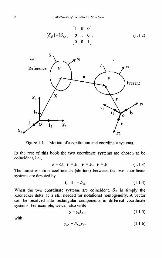
Consider a deformable continuum which, in the reference configuration at time to, occupies a region V with a boundary surface S (see Figure 1.1.1). N is the unit exterior normal of S. In this state the body is free from deformation and fields. The position of a material point in this state is denoted by a position vector X = XKlK in a rectangular coordinate system XK- XK denotes the reference or material coordinates of the material point. They are a continuous labeling of material particles so that they are identifiable. At time t, the body occupies a region v with a boundary surface s and an exterior normal n. The current position of the material point associated with X is given by y = y$k, which denotes the present or spatial coordinates of the material point.
Since the coordinate systems are othogonal,
**•»/=<*«» 1K'IL=8KL> (1-1-1)
where <5jw and 8KL are the Kronecker delta. In matrix notation,
l
2 Mechanics of Piezoelectric Structures
[8kl} = [8KL} =
"1 0 0"
0 1 0
0 0 1 (1.1.2)
to:
Reference
Present
Figure 1.1.1. Motion of a continuum and coordinate systems.
In the rest of this book the two coordinate systems are chosen to be coincident, i.e.,
o = 0, ii = I,, i2 = h, i3 = I3. (1.1.3) The transformation coefficients (shifters) between the two coordinate systems are denoted by
h-h=*kL- (1-1-4)
When the two coordinate systems are coincident, SUL is simply the Kronecker delta. It is still needed for notational homogeneity. A vector can be resolved into rectangular components in different coordinate systems. For example, we can also write
y=yKh, (1.1.5) with
yu=sulyi- (i-1-6)
Three-Dimensional Theories 3
The motion of the body is described by yt =yi(JL,t) . The equations of motion and Gauss's equation of electrostatic (the charge equation) are
KLj,L+Pofj =Po'yj: (1.1.7)
where KLj is the two-point total stress tensor, fo is the reference mass
density, fi is the mechanical body force per unit mass, and <D K is the
reference electric displacement vector. pE, a scalar (E is not an index), is the free charge density per unit reference volume, and a superimposed dot represents the material time derivative
D2yt d2yi(X,t)
yt Dtl dt2 (1.1.8) X fixed
In Equation (1.1.7), KLj and <D K are given by:
KLJ=FLj+MLj,
1 FLJ = yjjcTL MLJ = -^LME.EJ --EkEkS„), (1.1.9)
J = det(yiK), T, KL Po dy/
s7~ Et=-4>,
KL
and
<DK= e0JXKJD, = e0JC£zL + <PK,
yLKEi=-<t>K, (PK=JXK,PI
(1.1.10)
<E -Po dy/
d<Ev
where 6o is the electric permittivity of free space, Et is the electric field, Pt is the electric polarization per unit present volume, and D, is the electric displacement vector. <E K is the reference electric field vector,
and <PK is the reference electric polarization vector. <f> is the electric
potential. C]}L is the inverse of the deformation tensor, y/ = y/{SKL,cEK)
is a free energy density per unit mass, which is a function of <E K and the
4 Mechanics of Piezoelectric Structures
following finite strain tensor:
SKL={yi,Kyl,L-sKL)i2. ( l . i . i i )
From Equations (1.1.9) and (1.1.10), we have
KLJ =yj,KPoT^- + JXL,i£o(EiEj --EkEkSy), (1.1.12)
1 rr~ „ d¥ cDK=£0JC-lL<EL-p0
d<EK
With successive substitutions from Equations (1.1.9) through (1.1.11), Equation (1.1.7) can be written as four equations for the four unknowns y,(X,t) md<f>(X,t).
The free energy \j/ that determines the constitutive relations of nonlinear electroelastic materials may be written as
PQW(SKL^K)
~ „ £ SABSCD eABC^A^BC - X ^A^B
2 2 ABCD 2 2 AB
1 1 + T? SAB$CDSEF + „ * ^A^BC^DE
6 3 ABCDEF 2 1 /!BC£>£
_ 1 _ 1_ ~~ZUABCD
CEACEBSCD X '^•A'^B^'C
2 O 3 ABC
! (1.1.13)
+ "7 , ^ ^BC ^D£ ^FG 6 2 ABCDEFG
+ -a <EA<EBSCDSEF+-k <EA<EB<ECSDE 4 1 ABCDEF 6 3 /1BCD£
_ ~ Z ^A^B^C^D H '
where the material constants
2/!flCD 2 ^ B
C > * bABCD> X , (1.1.14) 3ABCDEF \ ABCDE 3 ABC
c , k , a , k , x 4ABCDEFGH 2 ABCDEFG 1 ABCDEF 3 ABCDE 4 ABCD
Three-Dimensional Theories 5
are called the second-order elastic, piezoelectric, electric susceptibility, third-order elastic, first odd electroelastic, electrostrictive, third-order electric susceptibility, fourth-order elastic, second odd electroelastic, first even electroelastic, third odd electroelastic, and fourth-order electric susceptibility, respectively. The second-order constants are responsible for linear material behaviors. The third- and higher-order material constants are related to nonlinear behaviors of materials.
For mechanical boundary conditions S is partitioned into Sy and ST, on which motion (or displacement) and traction are prescribed, respectively. Electrically S is partitioned into S^ and So with prescribed electric potential and surface free charge, respectively, and
SyvST=S,uSD=S, y f (1.1.15)
SynST=S,nSD=0.
The usual boundary value problem for an electroelastic body consists of Equation (1.1.7) and the following boundary conditions:
(1.1.16)
where y, and ^ are the prescribed boundary motion and potential, Tt is
the surface traction per unit undeformed area, and <JE is the surface free
charge per unit undeformed area. Consider the following variational functional:
y,
<t>--= y,
--$
KLkNL
<DKNK
on
on
= Tk
Sy,
S*>
on
= -aE or
Sr,
sD,
1 . .
dV (1.1.17)
+ [dt\ T,yidS-[dt\ aE<f>dS,
where
^(SKL,<EK) = -e0JEkEk =-e0JC^N<EM<EN. (1.1.18)
6 Mechanics of Piezoelectric Structures
The admissible yt and (j) for n satisfy the following initial and boundary conditions on Sy and S„>:
# , L 0 = 0, dy,\t=h = 0 in V,
yi=y, on S,, f 0 < / < / „ (1.1.19)
^ = ^ on S^, f0 < f < ^.
Then the first variation of fl is
(1.1.20)
- f dt\ {(DLNL+aE)S4dS.
Therefore the stationary condition of FT implies the following equations and natural boundary conditions:
KLk,L+Pofk=Poyk in V,
VK^PE i n V>
KlkNL=Tk on ST,
<DKNK=-vE on SD.
(1.1.21)
Denoting
KIM-WJU, fM=fjSfl4, TM=T,SiM, (1.1.22)
we can write Equation (1.1.7)i and Equation (1.1.20) as
K-iMj.+PJu=PoyM> (1.1.23)
and
< 5 n = f' dtL kKLM,L +PO/M -Poyu)^M
- f dt\ {cDLNL+aE)8(f>dS.
(1.1.24)
''0 *°D
Three-Dimensional Theories 1
1.2 Linear Piezoelectricity for Weak Fields
In linear theory, we introduce the small displacement vector u = y -X and assume infinitesimal displacement gradient and electric potential gradient. The infinitesimal strain tensor is denoted by
S»=\(MlJc+uki). (1.2.1)
The material electric field becomes
<EK=EiyitK=EiSlK->Ek. (1.2.2)
Similarly,
MLJ=0, KLJ=FLJ, <PK^Pk, <DK^Dk. (1.2.3)
Since the various stress tensors are either approximately zero (quadratic or of higher order in the infinitesimal gradients) or about the same, we use Ty to denote the stress tensor that is linear in the infinitesimal gradients. This notation follows the IEEE Standard on Piezoelectricity [3]. Our notation for the rest of the linear theory will also follow the IEEE Standard. Then
KU=FU^TV, TsKL^Tkl. (1.2.4)
For small fields the free energy density can be approximated by
p0y/{SKL,<EK)--s0JEkEk
= 2c2ABCD
S^cn-eABcZASBC
1 1 ( 2 }
—ZX cZA<EB--s<iJEkEk 2. 2 AB 2.
where
2cijklSijSkl ~eijkEiSjk ~'Z£ijEiEj ~H(Skl>Ek\
4=X +c0S„. (1.2.6) 2 ij
The superscript E in cijk, indicates that the independent electric
constitutive variable is the electric field E. The superscript S in sfj
indicates that the mechanical constitutive variable is the strain tensor S.
g Mechanics of Piezoelectric Structures
In Equation (1.2.5) we have also introduced the electric enthalpy H. The constitutive relations generated by H are:
dH E Ty - ~TZ- - CijklSkl ekijEk >
iJ (1.2.7) Di = —T7T = eiklSkl + £ikEk •
dEt
The material constants in Equation (1.2.7) have the following symmetries:
(1.2.8) cijkl -°jikl -cklij>
ekij = ekji i £ij ~ £ji •
We also assume that the elastic and dielectric material tensors are positive-definite in the following sense:
c!uSuSuZ0 for any S^Sj,,
and c J , V B = 0 => SiJ=0, ^ ^
£$EiEjZ0 for any E,,
and efjE,Ej = 0 => E,=0.
Similar to Equation (1.2.7), linear constitutive relations can also be written as [3]
T =rD,.S., -h...n. . (1.2.10)
(1.2.11)
T«-
Et-
sv
A
-rD V • ~ cijklc>kl
= ~"ikl^kl
= sijkl^kl
= "ikl^kl
-KjDk,
+ P?kDk,
+ dkijEk>
+ £lEk> and
Sij = Sijkl*kl + SkijDk '
The equations of motion and the charge equation become
A,, =Pe>
(1.2.12)
(1.2.13)
Three-Dimensional Theories 9
where p is the present mass density, and pe is the free charge density per unit present volume. The difference between p and po, and that between pE and pe are neglected in Equation (1.2.13).
In summary, the linear theory of piezoelectricity consists of the equations of motion and charge (1.2.13), the constitutive relations
*ij - Cijkl^kl ' ekijEk>
Di=eijkSjk+£,jEj,
(1.2.14)
where the superscripts in the material constants in Equation (1.2.7) have been dropped, and the strain-displacement and electric field-potential relations
With successive substitutions from Equations (1.2.14) and (1.2.15), Equation (1.2.13) can be written as four equations for u and </>:
(1.2.15)
cijkiuk,ij + eko<P,kj +ffi= pi*i>
e,klUkM~£iAu =Pe-
(1.2.16)
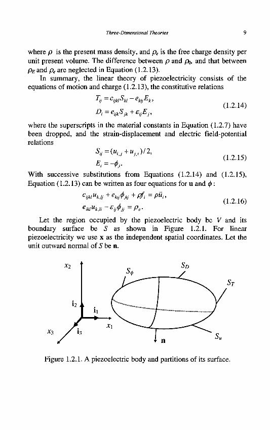
Let the region occupied by the piezoelectric body be V and its boundary surface be 5 as shown in Figure 1.2.1. For linear piezoelectricity we use x as the independent spatial coordinates. Let the unit outward normal of S be n.
*3
Figure 1.2.1. A piezoelectric body and partitions of its surface.
10 Mechanics of Piezoelectric Structures
For boundary conditions we consider the following partitions of S:
SuuST=S,uSD=S, ( i 2 i 7 )
SunST=S0nSD=O,
where Su is the part of S on which the mechanical displacement is prescribed, and ST is the part of 5 where the traction vector is prescribed.
S^ represents the part of S which is electroded where the electric
potential is no more than a function of time, and SD is the unelectroded part. We consider very thin electrodes whose mechanical effects can be neglected. For mechanical boundary conditions we have prescribed displacement ut
Uj -ui on Su, (1.2.18)
and prescribed traction tj
Tyni=tj on ST. (1.2.19)
Electrically, on the electroded portion of S,
<j> = lj> o n S , , (1.2.20)
where <j> does not vary spatially. On the unelectroded part of S, the charge condition can be written as
Djnj=-o:e on SD, (1.2.21)
where ae is the free charge density per unit surface area.
On an electrode S^ the total free electric charge Qe can be represented by
g e = f -n,DtdS. (1.2.22)
The electric current flowing out of the electrode is given by
I = -Qe. (1.2.23)
Sometimes there are two (or more) electrodes on a body that are connected to an electric circuit. In this case, circuit equation(s) will need to be considered.
The equations and boundary conditions of linear piezoelectricity can be derived from a variational principle. Consider [4]
Three-Dimensional Theories 11
-pu,u, - / / ( S , E ) + / / (M, -pj U(u,<f>)= f dt[
+ t dt f lutdS- f' <# f avfli^S'.
rfK (1.2.24)
u and 0 are variationally admissible if they are smooth enough and satisfy
du, I, = du, I, = 0 in V,
ui=ui on Su, tQ<t<tx, (1.2.25)
<^-(j> on S^, t0 <t<tx.
The first variation of fl is
m = f' dt I [(TJU +pfl-pui )dui + (Dtl - pe )5<f\dV
- p dt \ {T^j -t^Su^S- p dt f (D,n, + ae)S<f>dS. JtQ JST JtQ JSD
(1.2.26)
(1.2.27)
Therefore the stationary condition of Tl is Tjij + tfi = put in V, t0<t<tx,
Dt,i=Pe in V, t0<t<tx,
Tjinj=ii on ST, t0<t<t{,
Dini = -ae on SD, t0<t<tx.
We now introduce a compact matrix notation [3,4]. This notation consists of replacing pairs of indices ij or kl by single indices p or q, where i, j , k and I take the values of 1, 2, and 3, and p and q take the values of 1, 2, 3, 4, 5, and 6 according to
ij or kl: 11 22 33 23 or 32 31 or 13 12 or 21
porq: \ 2 3, 4 5 6
Thus T„. (1.2.29)
(1.2.28)
Cijkl ~* Cpq' e'1 e T ' i t / ' "ip' - y ' * p
For the strain tensor, we introduce Sp such that
S\=SU, S2=S22, S3=S33,
S4=2S23, S5=2S3l, S6=2Sl2. (1.2.30)
12 Mechanics of Piezoelectric Structures
The constitutive relations in Equation (1.2.7) can then be written as
Tp ~ CpqSq -ekpEk>
A eiqSq +£ikEk-
In matrix form, Equation (1.2.31) becomes
A A
f4
CE
c 3 1
'41
^51
VC61
'31
'12
'22
'32
'42
'52
-62
'12
'22
'32
'23
'33
'43
'53
' 63
= 13
'23
= 33
'14
'24
'34
'44
'54
'64
= 14
= 24
= 34
' 25
'35
'45
'55
'65
= 25
= 35
,E\ '16
-26
'36
' 46
'56
' 6 6 /
5,
= 12
= 14
\e\6
_ 16
26
3 6 .
>v s2 s, s, S5
• +
'3\
'22
= 23
= 24
= 25
= 26
M2
-.22
-32
(1.2.31)
= 32
= 33
= 34
= 35
-36 J
-13
;22
'33
(1.2.32)
1.3 Linear Theory for Small Fields Superposed on a Finite Bias
The theory of linear piezoelectricity assumes infinitesimal deviations from an ideal reference state of the material in which there are no preexisting mechanical and/or electrical fields (initial or biasing fields). The presence of biasing fields makes a material apparently behave like a different material, and renders the linear theory of piezoelectricity invalid. The behavior of electroelastic bodies under biasing fields can be described by the theory for infinitesimal incremental fields superposed on finite biasing fields [5,6], which is a consequence of the nonlinear theory of electroelasticity. This section presents the theory for small fields superposed on finite biasing fields in an electroelastic body.
Consider the following three states of an electroelastic body (see Figure 1.3.1).
Three-Dimensional Theories 13
Initial
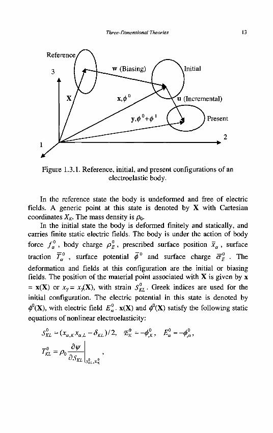
Figure 1.3.1. Reference, initial, and present configurations of an electroelastic body.
In the reference state the body is undeformed and free of electric fields. A generic point at this state is denoted by X with Cartesian coordinates XK. The mass density is p0-
In the initial state the body is deformed finitely and statically, and carries finite static electric fields. The body is under the action of body
force f£ , body charge pi, prescribed surface position xa , surface
traction T^ , surface potential ^° and surface charge a\ . The
deformation and fields at this configuration are the initial or biasing fields. The position of the material point associated with X is given by x
= x(X) or xY - x/X), with strain S^L • Greek indices are used for the initial configuration. The electric potential in this state is denoted by
0°(X), with electric field E°. x(X) and 0°(X) satisfy the following static equations of nonlinear electroelasticity:
S°KL=(xa,KxatL-SKL)/2, <E°K=-<f>°K, E°a=-£,
dy/ TKL = A)
55, KL &.&
14 Mechanics of Piezoelectric Structures
J°=det(xaK),
KL =xaA+<a, K=sQjGxKAxL<yL+<p\,
Ka = J°XK^0(EX -X-E»E»rSpa),
In the present state, time-dependent, small, incremental deformations and electric fields are applied to the deformed body at the initial state.
The body is under the action of ft , pE, yt,Tt , <f> and aE . The final position of X is given by y = y(X,/), and the final electric potential is 0(X,f). y(X,/) and 0(X,/) satisfy the dynamic equations of nonlinear electroelasticity:
So. = (y>,Kyt,L So.)12, <EK = -<t>tK, E,=-t
KLJ = yj,KTlL + MLj, CD K= £0JCK[<EL + cpK,
TKL=P<> dS KL SKL&K
(1.3.2)
MLj = JXL,i£0 (EiEj ~^EkEkSij )>
KLj,L + Pofj = Pofj . ®K,K=PE-
Let the incremental displacement be u(X,t) and the incremental potential be <l>l(X,t) (see Figure 1.3.1). u and (j)1 are assumed to be infinitesimal. We write y and (j) as
yi(X,t) = Sia[xa(X,t) + ua(X,t)], 3
Then it can be shown that the equations governing the incremental fields u and 01 are
KKa,K + Pofa = PoUa > ,. - ..
®K,K=PE>
Three-Dimensional Theories 15
where fxa and p\ are determined from
Ji ~°ia\Ja +Ja)> ,, -, <-s
o , i U - J - J ;
PE=PE+PE>
and the incremental stress tensor and electric displacement are given by the following constitutive relations:
:Lr K?„ -(jLyMauaM RMLy'EM,
K=RKLyUy,L+LKL'E[, (1.3.6)
where <ElK =-$K • Equation (1.3.6) shows that the incremental stress
tensor and electric displacement vector depend linearly on the incremental displacement gradient and potential gradient. In Equation (1.3.6),
^KaLy ~ XaM A ) aV
dSrudS,
R
>KMU°LN
+ TKL5ay+SKaLy =G
9 >
y,N
LyKa'
KLy -Po wKdsML
2
XyM + rKLy > SKL .%
LKL ~ Po 5 >
S'EK^L
+ 'KL ~ ^LK •
where
gfCaLy ~ S<)J \-EaEp(XK,pXL,y ~XK,yXL,p)
• F° F° X X ^a^y^- K,p^- L,p
r0 r 0
(1.3.7)
+ EpEr (XKaXLp - XKJ)XLja)
+ -^EpE<i(XK,rXL,a ~XK,aXL,y)\
YKLy ~£QJ (EaXK,aXL,y ~EaXK,yXL,a ~ Ey X K,aX L,a)>
(1.3.8)
'•KL ~ £<)J XKaXLa.
16 Mechanics of Piezoelectric Structures
GKaLy , RKLy , and LKL are called the effective or apparent elastic,
piezoelectric, and dielectric constants. They depend on the initial deformation x«(X) and electric potential 0°(X).
In summary, the boundary value problem for the incremental fields u and (j)1 consists of the following equations and boundary conditions:
KKaJC + Pofa = PoUa m V>
KLy = GLyMaUaM + RMLy<S>M i n V>
®\=RKLyUy,l-L^\ ™ V,
"a=Ua
?=? KlNL
<D\NK
on
on
=n =-4
Sy>
S*>
on ST,
on SD
Consider the following variational functional:
.1 . . 2 2
n(u,<l>X)=[tdt £ (-p0uaiia --GKaLyuKauLy
jrl „ , 1 , . ! / ! , „ /•! , 1 As
+ \''dt\ TxauadS-Ut\ a^dS.
(1.3.9)
•RKLy<t>Wy +-LKLP,KP,L+Pof>a-PEf)dV (1-3.10)
The admissible u and (j)1 must satisfy
ua=ua on Su, t0<t<tx, (1.3.11)
^ = ^ ' on 5 . , t0<t<tv
Three-Dimensional Theories 17
The first variation is found to be
ai(u, <p) = f' dt f [(K[aL + pX - Poua )Sua
(1.3.12) - £ d t l (K[aNL~Tx)SuadS
- f'df f {<DxKNK+ax
E)8<pdS. ' '0 "°£>
Therefore the stationary condition of the functional gives the following governing equations and boundary conditions:
Denoting
KL,K + Pofa = Po«a i n F>
®lK,K=Pl in V,
KlNL=Tx on ST,
(DlKNK=-al
E on SD.
*M =TaoaM, uM =uaoaM,
(1.3.13)
(1.3.14)
(1.3.15)
we can write Equation (1.3.12) as
<5TI(u, ) = [ dt [ [{Kluj, + pQfM - p0iiM )Suu
-£dtb {KxmNL-f^)duMdS
-£dt\ (cDxKNK+al
E)S<{>ldS.
In some applications, the biasing deformations and fields are also infinitesimal. In this case, usually only their first-order effects on the incremental fields need to be considered. Then the following energy density of a cubic polynomial is sufficient:
18 Mechanics of Piezoelectric Structures
1 _ 1 POV\^KL^K)-'ZCABCD^AB^CD ~eABC^A^BC ~~ZZAB^A^B
+ ~7C ABCDEFSAB$CDSEF
+ 'Z^ABCDE'^A^BC^DE (1.3.16)
n. "ABCD^A^B^CD f- ZABC^A^B^C'
where the subscripts indicating the orders of the material constants have been dropped. For small biasing fields it is convenient to introduce the small displacement vector w of the initial deformation (see Figure 1.3.1), given as
xa=SaKXK+wa. (1.3.17)
Then, neglecting the quadratic terms of the gradients of w and 0°, the effective material constants take the following form [5,6]:
^KaLy = CKaLy + CKaLy '
RKLy=eKLy+eKLy> (1.3.18) vKLy ~ cKLy ^cKLy>
LfCL ~ £KL + £KL '
where
(1.3.19)
CKaLy =^KL^ay +CKaLNWy,N +cKNLyWa,N
+ CKaLyAB$'AB + ^AKaLy^A >
eKLy ~eKLMWy,M ~ ^KLyAB^AB +"AKLy^A
+ e0(<E°KSLr-<EQL5Ky-<E0
MSMrSKL),
£KL =°KLABSAB + XKIA^-A + £O(SMM"KL ~2SKL),
1 KL ~CKLAB^AB ^AKL^A'
S°AB=(WA,B+WB,A)/2>
EjC =-<P,K-
In certain applications, e.g., buckling of thin structures, consideration of initial stresses without initial deformations is sufficient. Such a theory is called the initial stress theory in elasticity. It can be reduced from the theory for small fields superposed on a bias. First we set x = X. Furthermore, for buckling analysis, a quadratic expression of y/ with
Three-Dimensional Theories 19
second-order material constants only and the corresponding linear constitutive relations are sufficient. The biasing fields can be treated as infinitesimal fields. Then the effective material constants sufficient for describing the buckling phenomenon take the following simple form:
^KccLy ~ CKaLy + ^KL^ay
RKLY =eKLr+e0CE0KSLy -<E°L6Kr -<EMSMySKL), (1.3.20)
^KL = EKl'
where TKL is the initial stress and <EK is the initial electric field.
1.4 Cubic Theory for Weak Nonlinearity
By cubic theory we mean that effects of all terms up to the third power of the displacement and potential gradients or their products are included [7]. Cubic theory is an approximate theory for relatively weak nonlinearities, and can be obtained by expansions and truncations from the nonlinear theory in the first section of this chapter. The resulting equations are:
FLj=SJM x l
C UA,B+eALM<P,A+-C UK,AUK,B 2LMAB 2 2LMAB
2LKAB '"'"• " ' " 21LMABCD "r C UiA fWj H + C UA gUcD
+ eALKUM,K<t>,A ~ d UBC(j)A --bABLM<f>A<t>B
1 ABCLM 2
\_ ]_ + i £ , . UM,RUK,AUK,B + ~C UM,KUA,BUCD
2 2LRAB 2 3LKABCD 1 1
H C XI A RWJP- fXlis r) H C i 2HMABcD • • ' 6MMABCDEF
~d> ^,„UB.CUM,K<I>,A —zd UKBUKC<f>A
1 ABCLK 2 1 ABCLM
~ ^ i „ D ™ r , „ UB,CUD,E0,A ~-hABLKUM,K<l>,A<t>,B
1 1 +T« „ HC.D^.B+7^ Mate
2 1 ABCDLM 6 3 ABCLM
(1.4.1)
20 Mechanics of Piezoelectric Structures
(pL=eLBC^B,C X r,A +~ZeLBCUK,BUK,C 2 AL 2
O i , D™,- UB,CUD,E "ALCDUC,D^,A z, * LBL.DE
6 2 ZJJCDfiFG B ' C D ' £ F'G 2 MCD ' ' 'A
1 , 1 . + T ? „ , „ , , „ . UC,DUE,F<P,A + - « UD,E<P,A<P,B
2 1 ALCDEF 2 3 /fBLD£
O 4 ^BCL
(1.4.2)
^L/ = « o V # L # M _ ^ <*U #JC iW - # * # M MK,L
-<t>,K<l>MUL,K +^JMUK,K ~ W , KUK,M
+ <t>,K<f>,RUR,KSLM +-<l>,K<t>,KULM ~' ~4\R4»,««'K JC*>LM
(1.4.3)
£0JCA'EK =£o[-<f>,L + <f>,KUL,K -<f>,LUK,K +<f>,KUK,.
Y,MUL,KUKM +Y,KUM,MUL,K ~ Y,LUK,KUM,M
+ ~Zr,LUK,MUM,K ~r,MUL,KUM,K
(1.4.4)
+ <P,MUM,LUK,K ~r,MUM,KUK,L\-
A special case of cubic theory is the case of relatively large mechanical deformations and weak electric fields [8]. In this case all electrical nonlinearities can be neglected. The following energy density is sufficient:
Po¥ ~~ ~ CABCD^AB^CD eABC^A^BC ~ XAB^A^B
+ T CABCDEF $AB $CD $EF + T T CABCDEFGH $AB $CD SEF SGH • O z 4
(1.4.5)
Three-Dimensional Theories 21
Keeping the linear terms of the electric potential gradient and up to cubic terms of the displacement gradient, we obtain
K-UA ~CIMRSUR,S +eKLM<P,K
+ CLMRSKNUR,SUK,N +CLMRSKNUUR,SUK,NUI,J> (1.4.6)
where
®K-eKRSUR,S £KLY,L>
CLMRSKN - ~ \CLMRSKN + CLMNS°KR + CLNRS°KM )>
CLMRSKNU =~7CLMRSKN1J (1-4.7) O
+ T \CLMKNSJ °RI + CLNSJ °MK °RI + CLNRSIJ °MK )•
Chapter 2
Piezoelectric Plates
In this chapter we derive two-dimensional equations for a piezoelectric plate. First we examine a few exact solutions of vibration modes and propagating waves in plates from three-dimensional equations. They provide guidance in developing two-dimensional theories and serve as criteria for determining the accuracy of two-dimensional theories. Then two-dimensional plate equations are systematically derived.
2.1 Exact Modes in a Plate
The specific three-dimensional problems to be examined are the thickness-shear vibration of a quartz plate [10] and waves propagating in a plate of polarized ferroelectric ceramics [11,12].
2.1.1 Thickness-shear vibration of a quartz plate
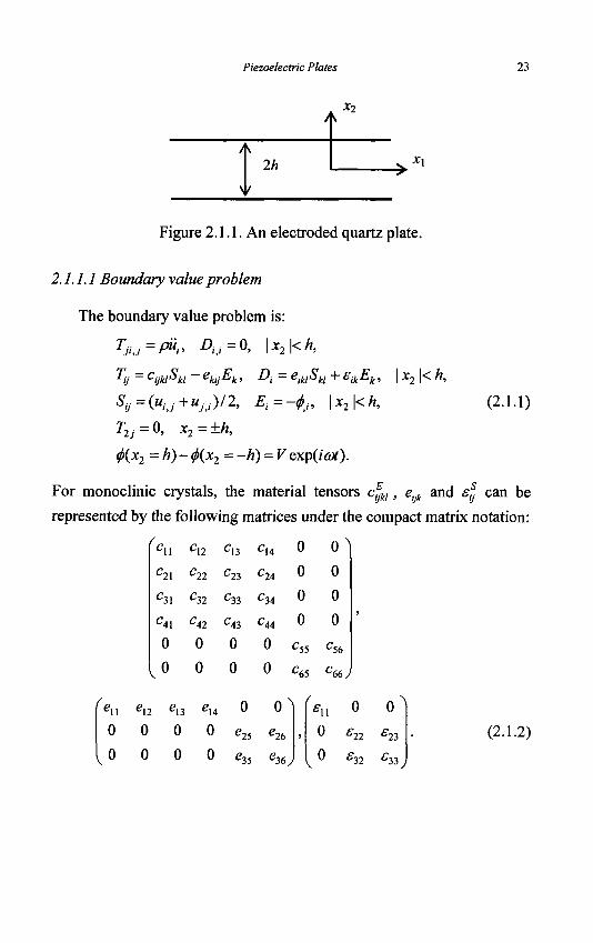
Quartz of crystal class 32 is probably the most widely used piezoelectric crystal. Plates of rotated Y-cut quartz [4] are particularly useful for thickness-shear resonators, filters, and sensors because of the existence of pure thickness-shear modes and their frequency stability. Langasite and some of its isomorphs (langanite and langatate) are emerging piezoelectric crystals which have stronger piezoelectric coupling than quartz and also belong to crystal class 32. Rotated Y-cut quartz exhibits monoclinic symmetry of class 2 (or C2) in a coordinate system (xijc2) in and normal to the plane of the plate. Consider an unbounded, rotated Y-cut quartz plate (see Figure 2.1.1). The two major surfaces are traction-free and are electroded, with a driving voltage Vexp(ia>t) across the thickness.
22
Piezoelectric Plates 23
X2
2h X\
Figure 2.1.1. An electroded quartz plate.
2.1.1.1 Boundary value problem
The boundary value problem is:
Tjij=Pui> A,/=0> l*2l<*»
Ty - cijkt^ki ~ ekij-Ek > A = eiki^ki + £tk^k > \ x i \ < n>
Sy=(uij+uj,i)/2> Ei=-<l>,i> \x2\<K
l2j 0, •±h,
0ix2 -h)-0(x2 = -h)- Vexp(ia>t).
(2.1.1)
For monoclinic crystals, die material tensors cfjkl, ejjk and efj can be
represented by the following matrices under the compact matrix notation:
'13
^21
C41
0
0
u22
C32
C42
0
0
23 C
c43
0
0
•-14
C24
C34
C44
0
0
0
0
0
0
C55
^65
0
0
0
c56
C667
0
0
0
0
c13
0 "=14
0
0
0 0}
'25
c35
c26
'367
c l l
0
0
0 0
'22
'32
'23
'33
(2.1.2)
24 Mechanics of Piezoelectric Structures
Consider the possibility of the following displacement and potential fields:
"i = ux(x2)exp(icot), U2=UT,= 0,
^ = ^(*2)exp(i<ar).
The nontrivial components of strain, electric field, stress, and electric displacement are
2Sn=ul2, E2=-<j>2, (2.1.4)
and
^31 = C56M1,2 + e25^,2> ^12 = C66M1,2 + e26r,2> ^ ,>
A> = g26Ml,2 - £22^,2> A = e36Ml,2 ~ £23#2 >
where the time-harmonic factor has been dropped. The equation of motion and the charge equation require that
^21,2 = C66W,,22 + e26^,22 = ~PG)\ , « . „
(2.1.6) -^2,2 = g26Ml,22 ~ f22r,22 = ^-
Equation (2.1.6)2 can be integrated to yield
<l> = ux+Bxx2+B2, (2.1.7) f22
where Bx and B2 are integration constants and B2 is immaterial. Substituting Equation (2.1.7) into the expressions for T2\, D2, and Equation (2.1.6)1, we obtain
^21 = C66"l,2 + e26^1> A> = - £ 2 2 5 1 » ( 2 . 1 . 8 )
^66M1,22 = _ P G , 2 " l ' ( 2 - 1 - 9 )
where
c66=c66(l + k226), &=-&-. (2.1.10)
f22C66
Piezoelectric Plates 25
The general solution to Equation (2.1.9) and the corresponding expression for the electric potential are
ux = Ax sin §c2 + A2 cos<£c2,
tf> = -^(Ax sin <!pc2 + A2 cos fy2) + Bxx2 +B2, (2.1.11)
'22
where A i and^2 are integration constants, and
?=-?-a)2. (2.1.12) C66
Then the expression for the stress component relevant to boundary conditions is
Ti\ =c6 6(4£cos£;2 - ^ s i n ^ + e ^ . (2.1.13)
The boundary conditions require that
c66A£ cos #i - c66A2^ sin & + e26Bx = 0,
c66 Ax£, cos £h + c66A2^ sin gh + e26Bx = 0, (2.1.14)
2^Axsm%h + 2Bxh = V. £22
We can also add the first two, and subtract the first two from each other:
c^A^ cos Z;h + e26Bx=0,
c 6 6 ^ s i n ^ = 0, (2.1.15)
2^-Alsin^i + 2Blh = V. £22
2.1.1.2 Free vibration solution
First, consider free vibrations with V = 0. Equation (2.1.15) decouples into two sets of equations. For symmetric modes,
c66,42£sin£/z = 0. (2.1.16)
Nontrivial solutions may exist if
sin^/? = 0, (2.1.17)
26 Mechanics of Piezoelectric Structures
or
£n)h : nn , H = 0 , 2 , 4 , 6 , (2.1.18)
which determines the following resonant frequencies:
CO ,(») nn \CLC "?J—. "-0,2,4,6, 2/z
y , * - , - r ? \ / ? (2.1.19)
Equation (2.1.17) implies that B\ = 0 and ^ = 0. The corresponding modes are
uy = cos£(n);c2, </> = -^-cos^ (n)x2, (2.1.20) '22
where « = 0 represents a rigid body mode. For anti-symmetric modes,
c ^ ^ c o s ^ + e ^ ^ O ,
2 - ^ - 4 sin #r + 2fl,/r = 0. 522
The resonance frequencies are determined by
c66^cos^h e 26 c26 sin<fjfr 522
= c66^hcos^h —— sin J;h = 0, '22
(2.1.21)
(2.1.22)
or
where
tan^ = -p- , *26
(2.1.23)
P - ^26 c26 v26
f22C66 £22C66U "*" *26 ) 1 + «; 26
(2.1.24)
Equations (2.1.23) and (2.1.21) determine the resonant frequencies and modes. If the small piezoelectric coupling for quartz is neglected in Equation (2.1.23), a set of frequencies similar to Equation (2.1.19) with n equals odd numbers can be determined for a set of modes with sine
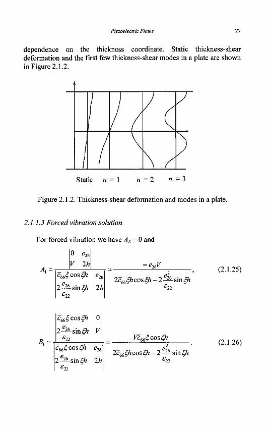
Piezoelectric Plates 27
dependence on the thickness coordinate. Static thickness-shear deformation and the first few thickness-shear modes in a plate are shown in Figure 2.1.2.
Static n = l w = 2 « = 3
Figure 2.1.2. Thickness-shear deformation and modes in a plate.
2.1.1.3 Forced vibration solution
For forced vibration we have A2 = 0 and
A =
o s26
V 2/z e26V c^cosgh e26
sin J;h 2h 2 .£26
£22
2c66£hcos£h-2^smZh £22
(2.1.25)
B,
c66 |cos#2 0
2 - ^ s i n ^ V e22
c66£cos|/z e26
sin EJi 2h 2f26 £22
Vc^cosZh
2c66^h cos Eft - 2 -22- sin h £22
(2.1.26)
28 Mechanics of Piezoelectric Structures
Hence
A 22 1 — 22 &
2h&-k£tmgi -°e, (2.1.27)
where ae is the surface free charge per unit area on the electrode at x2 = h. The capacitance per unit area is then
& V 2h
the following limits:
l imC = ^ s «26->o 2h
l i m C - * 2 2
«*-><> 2h
#-Jfc£tan#
1 = £22a-4 M
^)
1+fc 26
(2.1.28)
(2.1.29)
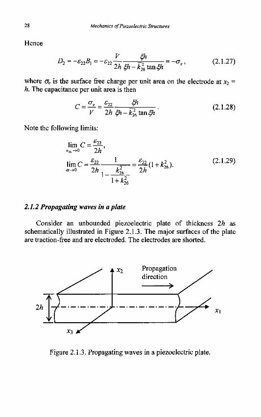
2.1.2 Propagating waves in a plate
Consider an unbounded piezoelectric plate of thickness 2h as schematically illustrated in Figure 2.1.3. The major surfaces of the plate are traction-free and are electroded. The electrodes are shorted.
x2 Propagation direction
Figure 2.1.3. Propagating waves in a piezoelectric plate.
Piezoelectric Plates 29
2.1,2.1 Eigenvalue value problem
We study straight-crested waves without x^ dependence. Then the homogeneous form of Equation (1.2.16) takes the following form:
C11M1,11 + C12M2,21 + C14W3,21 + C15M3,11 + C16VM1,21 + M 2 , l l )
+ C16M1,12 + C26M2,22 + C46M3,22 + C56M3,12 + C66VM1,22 + M2,12)
+ e i 6 ^ 1 2 + e 2 6 ^ , 2 2 = M '
C16M1,11 + C 2 6 M 2 , 2 1 + C46M3,21 + C56M3,11 + C 66V M 1,21 + W 2 , l l )
+ ei6<f>u+e26<p2i
+ CuUll2 +C22W222 + C24M3,22 + C25M3,12 + C 26V M 1,22 + M 2 , 1 2 )
+ e i 2 ^ , 1 2 + e 2 2 ^ 2 2 = / C ' " 2 '
C15M1,11 + C25M2,21 + C45W3,21 + C55M3,11 + C 56V M 1,21 + M 2 , l l )
+ e15^, l 1 + ^ 2 5 0 , 2 1
+ C14M1,12 + C24M2,22 + C44M3,22 + C45M3,12 + C46 (Ml,22 + M 2 , 1 2 )
+ e i 4 ^ , 1 2 + e 2 4 ^ , 2 2 : = / 9 " 3 '
e i l M l , l l + e i 2 M 2 , 2 1 + g 1 4 M 3 , 2 1 + e 1 5 M 3 , l l + e i 6 (Ml,21 + M 2 , l l )
- ^ 1 ^ 1 1 - ^ 1 2 ^ , 2 1
+ e2 lM l ,12 + g22M2,22 + g24M3,22 + e25M3,12 + e26VWl,22 + M2,12 )
— f 12r ,12 ~E22Y,22 = ^ -
We seek solutions representing waves propagating in the x\ direction:
"j(*,0 = exp(£??x2)exp[/(fa, -a*)] ,
^(x,/) = A4 exp(kTjx2)exp[i(kxx - <#)],
where k and ft) are the wave number in the x\ direction and the frequency, respectively. r\k is related to the wave number in the JC2 direction. Aj (j = 1, 2, 3) and As, are complex constants, representing the wave amplitude.
30 Mechanics of Piezoelectric Structures
Substitution of Equation (2.1.31) into Equation (2.1.30) leads to the following four linear algebraic equations for Aj and A*.
[pa2 + k2 (^2c66 + i2jjcl6 - c,, ) ]4
+ k2 (TJ2C26 + irjc66 + ir)ci2 - c16)A2
+ k2(TJ2C46 + i?]c56 + irjcu -cX5)A3
+ k2 (Ji2e26 + irje2X + irjeX6 - e,, )A4 = 0,
k2(rj2c26 + irjc2i + tyc* -cX6)Ax
+ [pco2+k2(jj2c22+i2T}c26 -c66)]A2
+ k2 (T]2C24 + irjc25 + irjc46 - c56 )A\
+ k2 {rfe22 + it]e26 + i?]en - eX6 )AA = 0
k2(rj2ci6 + iT]cu+irjc56 -cX5)Ax
+ k2 (rj2cu + irjc46 + ir]c2i - c56 )A2
+ [pco2 +k2(Tj2c44+ilr]c45 ~c55)]A3
+ k2 (/72e24 + iT]e25 + ir]eH - ex5 )AA = 0,
{t]2e26 + iT]e2x+irjeX6-en)Ax
+ (.n2e22 + iWin + i?1eu ~e\(,)Ai
+ (rfe24 + i?]e25 + iT]eX4 -ex5)A3 ^ ^
- ( ^ 2 2 +*2i7ff12 - c u H =0-
For nontrivial solutions ofv4y and/or A4, the determinant of the coefficient matrix of the above equations must vanish. This leads to a polynomial equation of degree eight for r\. We denote the eight roots of the equation by r\{m), and the corresponding eigenvectors by (^m),^44
(m)), m = 1, 2,
..., 8. Thus, the general wave solution to Equation (2.1.30) in the form of Equation (2.1.31) can be written as
8 _ ui = ZC(m)4 ( m ) e*P(kri{m)x2)exp[i(kxx - ox)\
mg=1 (2.1.33)
<* = SC('«)^t(m) ®cp(*»7(»,)*2)exP[*(**i ~ ** ) ! m=\
Piezoelectric Plates 31
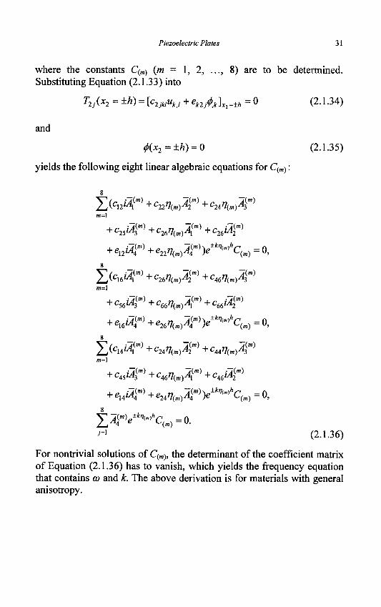
where the constants C(m) (m = 1, 2, ..., 8) are to be determined. Substituting Equation (2.1.33) into
T2J(x2 = ±h) = [c2jklukJ + ek2J£k]X2=±h = 0 (2.1.34)
and
<f>(x2=±h) = 0 (2.1.35)
yields the following eight linear algebraic equations for C(m):
8 _ _ _
2_J(cuiAl +c22rj(m)A2 + c24rj(m-)A3 m=\
-t-c25m3 -•-t-2677(m) j + c26m2
+ el2a\m) +e22r1{m)Aim))e±k^hC{m) = 0,
m=\
+ C56L^3 +C 6 6 77 ( m ) ^ , + C 6 6 M 2
-t- e 1 6 M 4 + e26T/(m)Ji4 ) e ^-(m) ~ U>
8 _ _ _
^(c14L4, +c24rj(m)A2 + c^ri^A^
+ c45iA^+c46i1{m)^+c46U<f)
+ eX4iA\m) +e24T}{m)A^)e±k^hC(m) = 0, s
7(m) ±*I7(„)A, 1 ^ * ^ c ( m ) = o . 7=1 (2.1.36)
For nontrivial solutions of Qm), the determinant of the coefficient matrix of Equation (2.1.36) has to vanish, which yields the frequency equation that contains co and k. The above derivation is for materials with general anisotropy.
32 Mechanics of Piezoelectric Structures
2.1.2.2 Numerical example
As a numerical example, consider a plate of polarized ceramics poled in the x^ direction with
0
0
h\
0
0
g31
\x C\2
Cl3
0
0
, 0
0
0
£33
C12
c l l
C13
0
0
0
0
«15
0
Cl3
^13
C33
0
0
0
£15
0
0
0 0
0 0
0 0
C44 0
0 C44
0 0
0"
0
0 ?
( «11
0
0
(O 0
0
0
0 C 66 ,
J
0 0"
*n 0 0 S33J
(2.1.37)
where c^ = (c\\ - C\2)I2. Polarized ceramics are transversely isotropic. Their linear behavior described by Equation (2.1.37) is the same as crystals of 6mm symmetry. For the above straight-crested waves, when
co I co
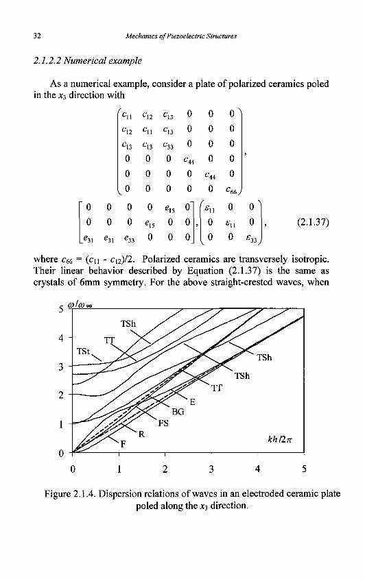
Figure 2.1.4. Dispersion relations of waves in an electroded ceramic plate poled along the x3 direction.
Piezoelectric Plates 33
the poling direction is along the x%, axis, u\ is coupled with w2, and W3 is coupled with 0, but the two groups do not couple to each other. The dispersion relations (co versus k) for PZT-5H are plotted in Figure 2.1.4.
There exist an infinite number of branches of dispersion relations. Only the first nine branches are shown. The wave frequencies are normalized by the lowest thickness-shear frequency
(2.1.38)
The dispersion relations are labeled as follows, along with the dominant displacement component at small wave numbers:
E = extension (wi),
F = flexure (w2),
FS = face-shear (z/3),
TSh = thickness-shear (u\),
TSt = thickness-stretch (1/2),
TT = thickness-twist (w3),
R = Rayleigh surface wave {u\ and u2),
BG = Bleustein-Gulyaev surface wave (W3).
In the figure, the three branches passing the origin are the so-called low frequency branches. They represent the extensional, flexural, and face-shear waves. The other six branches are high-frequency branches, which have finite intercepts with the (O axis. These intercepts are called cutoff frequencies, below which the corresponding waves cannot propagate. Cutoff frequencies are in fact the frequencies of pure thickness modes. The six high frequency branches shown represent three thickness-shear waves, one thickness-stretch wave, and two thickness-twist waves. One of the two dotted lines in the figure is the well-known Rayleigh surface wave, which can propagate over an elastic half-space and is not dispersive. The other dotted line is the well known Bleustein-Gulyaev surface wave which has only one displacement component z/3 and can propagate over a piezoelectric half-space but does not have an elastic counterpart. These two surface waves are included as references. It is seen that for short waves with larger k, the frequencies of the extensional
co„
34 Mechanics of Piezoelectric Structures
and flexural waves approach that of the Rayleigh surface wave. Similarly, for short waves, the frequencies of the face-shear wave approach that of the Bleustein-Gulyaev wave.
2.2 Power Series Expansion
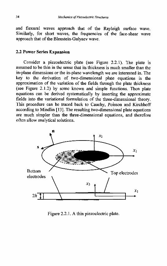
Consider a piezoelectric plate (see Figure 2.2.1). The plate is assumed to be thin in the sense that its thickness is much smaller than the in-plane dimensions or the in-plane wavelength we are interested in. The key to the derivation of two-dimensional plate equations is the approximation of the variation of the fields through the plate thickness (see Figure 2.1.2) by some known and simple functions. Then plate equations can be derived systematically by inserting the approximate fields into the variational formulation of the three-dimensional theory. This procedure can be traced back to Cauchy, Poisson and Kirchhoff according to Mindlin [13]. The resulting two-dimensional plate equations are much simpler than the three-dimensional equations, and therefore often allow analytical solutions.
Figure 2.2.1. A thin piezoelectric plate.
Piezoelectric Plates 35
2.2.1 Expansions of displacement and potential
2.2.1.1 Polynomial approximation of thickness modes
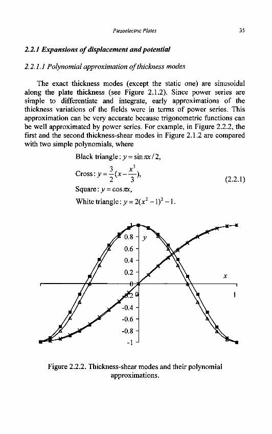
The exact thickness modes (except the static one) are sinusoidal along the plate thickness (see Figure 2.1.2). Since power series are simple to differentiate and integrate, early approximations of the thickness variations of the fields were in terms of power series. This approximation can be very accurate because trigonometric functions can be well approximated by power series. For example, in Figure 2.2.2, the first and the second thickness-shear modes in Figure 2.1.2 are compared with two simple polynomials, where
Black triangle: y = sin m 12,
3 *3
Cross: v = — (JC ), y 2V 3 (2.2.1)
Square: y = cos TDC, White triangle: y = 2(x2 -1)2 - 1 .
Figure 2.2.2. Thickness-shear modes and their polynomial approximations.
36 Mechanics of Piezoelectric Structures
2.2.1.2 Polynomial expansions
In a series of papers [14-17], Mindlin developed theories for high frequency vibrations of isotropic, anisotropic, and piezoelectric plates by power series expansions in the plate thickness coordinate. We now derive two-dimensional equations for a piezoelectric plate in the manner of [17]. First we expand the mechanical displacement and the electric potential into power series in xj,
00
"=0 (2.2.2)
Our goal is to obtain two-dimensional equations for u\n) and tf>(n). The lower order two-dimensional displacements can describe the following deformations:
Wj(0), «20) _ extension,
uf* - flexure,
u{l\u^- fundamental thickness-shear,
u^ - fundamental thickness-stretch,
wP),«22) - symmetric thickness-shear,
For piezoelectric device applications we want to derive plate equations that can describe the thickness-shear and thickness-stretch deformations well. It is important to note that these deformations have different behaviors in static and dynamic problems. For example, the first or fundamental thickness-shear mode of n = 1 in Figure 2.1.2 is sinusoidal along the plate thickness. However, the static thicken-shear deformation shown in the same figure is linearly varying along the plate thickness. Therefore the fundamental thickness-shear has different distributions along the plate thickness in static and dynamic problems. One simple expression can only approximate either the static or the dynamic deformation well, but not both.
Piezoelectric Plates 37
We are mainly interested in dynamic problems. Obviously the sinusoidal variation of the fundamental thickness-shear deformation can be well approximated by a cubic polynomial. However, we are not interested in accurately describing the field variation along the plate thickness. Our main goal is to develop plate theories than can predict the frequencies and dispersion relations of these modes accurately. For this
purpose, following Mindlin, we use a linear function x3u^\xux2,t), a = 1, 2, to approximately describe the fundamental thicken-shear motion. The main advantage of using a linear function is its simplicity. The error due to the approximation in resonant frequencies can be reduced or removed by introducing some correction factors. Overall this is a simple and accurate approach.
Shear correction factors are essentially not needed when using sinusoidal or higher-degree polynomial approximations for thickness-shear modes in the sense that the thickness-shear frequencies can be predicted exactly or accurately. This approach involves more algebra. In addition, the static thickness-shear behavior cannot be described well by a sine function or a cubic or higher-degree polynomial. Hence corrections may be needed for low frequency behaviors.
2.2.2 Strains and electric fields
From Equation (2.2.2) and the strain-displacement relation and the electric field-potential relation in Equation (1.2.15), we obtain
Sy=^Sf\ E^^E}*, (2.2.3) n n
where
W 4^"' + "V + {n +1)(<^"+1) + ^ M < " + I ) ) ] ' ( 2 . 2 4) EJn)=-</>f-(n + l)53/"
+l).
The first few orders of strains and electric fields have the following form:
e(0) _ „(0) v(0) _ (0) 9(0) _ (l)
38 Mechanics of Piezoelectric Structures
5<4,)=«g + 2«(2)
> ^ > = I4J> + 2II[2>, S ^ u g + ^ J . ( 2 '2 '6 )
e(2) _ ,.(2) r,(2) _ (2) - ( 2 ) _ ~ (3)
S f ^ a g + 3 1 ^ , 5<2>=i4J + 3a{3>, 5<a> = iig> +1^>, ( 2 ' 2 ' 7 >
E{0) = -<f>?\ E^ = -<j>f, £<°> = - / ' > , (2.2.8)
E{l) = -$\ £<» = -$>, £3(1) = - 2 ^ 2 ) , (2.2.9)
£ , ( 2 ) =-$ 2 ) . E?=-$\ £<2>=-30(3). (2.2.10)
The zero-order plate strains in Equation (2.2.5) describe homogeneous deformations of a plate element. The first-order strains in Equation (2.2.6) represent higher-order deformations of a plate element like curvature and twist, etc. Pictures of zero- and first-order deformed plate elements can be found in [13].
2.2.3 Constitutive relations
The plate resultants of various orders are defined by
7j"> = J * / ^ , A(n) = [hDiX"3dx3. (2.2.11)
Substituting the three-dimensional constitutive relations from Equation (1.2.14) into Equation (2.2.11), we obtain the plate constitutive relations as:
Iij _ Z J mn(- Ukl kl ekij£'k h
(2.2.12) D^=^Bmn(eiJkS^+evE^),
where
Bmn=\h x»x»dXiJ
2h /(« + » + lX « + » even, ^ ^ •>-* 0 . m + n odd. 0, m + n odd.
Piezoelectric Plates 39
Pictures of zero- and first-order plate resultants are given in [13]. They represent extensional and shear forces, and bending and twisting moments, etc.
2.2.4 Equations of motion and charge
We use the variational formulation in Equation (1.2.26) to derive the plate equations of motion and charge. For convenience we introduce a convention in which subscripts a and b assume 1 and 2 only but not 3. Let A be a two-dimensional area in the x\-x2 plane with a boundary curve C. Then Equation (1.2.26) can be written as
m= £ dt\A dAJ^ dx3[(Taja+ tfj-pujWj+T^&ij]
+ f dt\ dA\\ dx3[(Daa-pe)S<f> + DX3S<f,] J'; lA 7 (2.2.14)
- f dt[' dl\"dx^T^-tj)^
- f dt\ dl\h dx3(Dana + ae)S</>, J<o JCD J-h
where CT has prescribed traction and CD has prescribed surface charge. Substituting Equation (2.2.2) into Equation (2.2.14), with integration by parts with respect to x3 and time, we obtain
n ° V. m
+ Z t dt\ {D%-nDtl)+0M)5^dA Jtn JA
m)
J
SufdA
(2.2.15)
" Z \';dtj(T^na-I^)Sufdl
- Z {'dt\ (D^n^a^W dl,
40 Mechanics of Piezoelectric Structures
where the body and surface loads of various orders are defined by
Din) = K A ] - „ - \h_hPe*3dx3, (2.2.16)
^ = £ 0 * 3 * 3 . ^ B > = f / X * 3 -
For independent variations of du^n) and <5^(n), we obtain
7g-ii7g-I>+F<->=p2M") in ^
^-"r'+B^o in A ( 2 2 1 7 )
7}">»B=/;-> on Cr,
^">iiB=-a<-> on CD.
We note that electrodes in fact impose constraints on S<j)(n) [18]. This will be discussed in the next section.
In addition to power series expansions, it was pointed out in [13] that trigonometric series could also be used. Two-dimensional equations obtained from trigonometric expansions were given in [19-21]. More references on various expansions can be found in a review article [22]. In this book we mainly focus on power series expansions. We note that the following polynomial expansion of the electric potential [23]:
</> = ^(0) + x3<f>m + (x2 - h 2 ){(j)(2) + x 3 / 3 ) + • • •) (2.2.18)
has an important feature, i.e., only the first two terms do not vanish at
x^=±h. Therefore only ^(0) and tf>m are responsible for the voltage
across the plate thickness. Then in the plate equations of electrostatics only the zero- and first-order equations have surface charge terms. These will make it convenient for an electroded plate, especially for higher order equations.
Piezoelectric Plates 41
2.3 Zero-Order Theory for Extension
In this section we develop equations for extensional motions of thin plates. The propagation of extensional and face-shear waves is examined and compared with the three-dimensional solutions so that the range of applicability of the plate equations can be established. The equations are specialized to plates of polarized ceramics. As an example, the equations are used to study radial vibrations of a circular ceramic disk.
2.3.1 Equations for zero-order theory
By a zero-order theory we mean a theory for extensional motions of
a plate with w,(0) and i/<°> as the major displacements. For the electrical
behavior of the plate we are interested in what is governed by ^(0) and
$m. The approximate displacement and potential fields are
' ' 3 ' (2.3.1)
<f> = ^ + x3f\ Although we are mainly interested in w1
(0) and tip, we have included a
few other displacement components in Equation (2.3.1). Among these
additional displacements, u^ represents the thickness stretch or
contraction accompanying extension due to Poisson's effect, and must be
included, w^ describes flexure. w,(1) and u^ represent thickness-shear.
From Equation (2.2.5) it can be seen that w^0) together with u[{) and u^
contribute to thickness-shear deformations S^ and S^ , which may couple to extension due to anisotropy and should be allowed. The two-dimensional plate equations we will obtain are for the extensional
displacements w,(0) and M£0) . Other displacements will be eliminated through a stress relaxation procedure. Within the approximation in Equation (2.3.1), the strains and electric fields in Equations (2.2.5), (2.2.8) and (2.2.9) become:
e(0) _ ,.(0) o(0) _ (0) ?(0) _ (l)
o i o o i o o o (2-3"2)
O4 = I/3 2 + W2 ' "5 = ^ 3 1 ~*~ " l ' " 6 = "l 2 "** ^2 1 '
42 Mechanics of Piezoelectric Structures
E™ = -$\ 40)=-$\ E^=-f\ (2.3.3)
EF^-flK 4l) =-*$>, 4l) = 0. (2.3.4)
Higher order strains SJP are neglected.
From Equation (2.2.17)i, for 7 =1 ,2 and n = 0, we obtain
TZ+F^ = 2hpiif\ a,b = \,2, (2.3.5)
where we have truncated the right hand side by keeping the 5oo term only in the summation.
For the electrostatic equations we discuss several cases below. In the theory of piezoelectricity the electric potential is at most a function of time on an electrode. For example, if both the top and bottom surfaces of the plate are electroded, we can write
<b = VAt), x,=h, W l 3 (2.3.6) t = V2(t), x3=-h.
Since
we have
^ s ^ ( 0 ) + V ( 1 ) , (2.3.7)
Equation (2.3.8) imposes constraints in the variational formulation in Equation (2.2.15). These constraints can be systematically treated by the
method of Lagrange multipliers [18]. In our case with ^(0) and ^(1) only,
the constraints are relatively simple so we will proceed in the manner of [24,25]. We discuss four possibilities separately.
(i) An unelectroded plate
In this case S<j>^ and StfP are independent functions of x\, x2 and /.
We have the following two-dimensional equations of electrostatics:
Z><°>+JD(0)=0,
(2.3.9)
Dm-D^+Dm = o.
Piezoelectric Plates 43
(ii) A symmetrically electroded plate
In this case JC3 = ±h are both electroded. ^(0) and ^(1) are directly
determined by Equation (2.3.8) as functions of time. No differential
equations for ^(0) and ^(1) result from Equation (2.2.15) and no
differential equations are needed for determining ^(0) and ^(1).
(iii) A plate with the upper surface electroded From Equation (2.3.8)1
S<f>m + h8<f>m=0. (2.3.10)
Substituting Equation (2.3.10) into Equation (2.2.15) we obtain
- KDi0)a + Dm) + D% - D^ + Dm = 0. (2.3.11)
Since ^(0) and ^ are related by (2.3.8)1, we only need one differential
equation (2.3.11) to determine one of them. When the upper surface is electroded, D3(h) is unknown. Equation (2.3.11) can also be obtained by
eliminating D3(h) between Equations (2.3.9)i and (2.3.9)2. This procedure can also be used to treat prescribed displacement on a major surface of a plate when using two-dimensional equations [26].
(iv) A plate with the lower surface electroded From Equation (2.3.8)2
S<f>m-hS<f>m = 0. (2.3.12)
Substituting Equation (2.3.12) into Equation (2.2.15) we obtain
h(D(0) + Z )0>) ) + Z,(i) _D(o) +Dm = 0 j ( 2 . 3 . 1 3 )
which is equivalent to eliminating D3(-h) between Equations (2.3.9)i
and(2.3.9)2.
44 Mechanics of Piezoelectric Structures
For plate constitutive relations, we truncate Equation (2.2.12) by keeping the B0o and Bu terms only in the summation:
Tp = 2h(c,klSW-ekyEJ?),
D^^lhie^Sf+s^), (2.3.14)
nd) - ^ L £ £m
' ~ 3 a J '
where SJP have been neglected. Since S^0) contains w^0) and wf' ,
Equations (2.3.14) are not yet ready to be used for a theory of extension. To obtain the proper constitutive relations for extension we proceed as follows [13]. Since the plate is assumed to be very thin and for extension the dominating stress components are Tn, T& and Tn, we take the following to be approximately true:
7 j 0 ) = 0 . (2.3.15)
Equation (2.3.15) is called stress relaxation. According to the compact matrix notation, with the range of p, q as 1, 2, ... and 6, Equation (2.3.15) can be written as
rg( 0 )=0, 9 = 3,4,5. (2.3.16)
For convenience we introduce another index convention in which subscripts u, v, w take the values 3, 4, and 5 while subscripts r and s take the remaining values 1, 2, and 6. Then Equation (2.3.14)i>2 can be written as
T^=2h{crsST+CruST-ekrEf\
rv(0) = 2/*(cvA
(0) + c ^ - e ^ ) = 0, (2.3.17)
where Equation (2.3.16) has been used. From Equations (2.3.17)2 we have
%0)=-clcJir>+c2ekA°>. (2.3.18)
Piezoelectric Plates 45
Substitution of Equation (2.3.18) into Equations (2.3.17)1>3 gives
DP = 2h{WisS^ ^ijEf), ( -
where the material constants relaxed for thin plates are
Yrs ~ Crs ~ CrvCvwCws' f,S — 1,Z,0,
Wks = eh ~ tkwCvlcvs' v,w = 3,4,5, (2.3.20)
Gkj = £kj + ekvCvwejw J>* = 1>2,3.
In summary, in the case of an unelectroded plate, we have obtained
TZ+Fl0)=2hpuf\ a,b = 1,2,
D%+D^=0,
Dill-D^+Dm=0,
T^ = 2h(rrsSf) - ¥krE^\ r,s = 1,2,6,
DP = 2h(M,isSf) + Z,jEf\ (2.3.21)
C(0) _ „(0) -(0) _ (0) r.(0) _ (0) (0) "1 — "l,l > ° 2 ~~ "2,2 ' ° 6 — "1,2 + " 2 , 1 »
E[V=-$\ E^=-$\ E^ = -<f>m,
E™=-$\ E$> = -$\ ^ = 0 .
With successive substitutions from Equations (2.3.21)4.9, Equations
(2.3.21)i_3 can be written as four equations for u[°\ uf\ ^(0) and ^(1).
At the boundary of a plate with an in-plane unit exterior normal n and an in-plane unit tangent s (see Figure 2.2.1), we may prescribe
ri„0) or u™, r„f or ui°\
Di0) or </>m, D™ or f \
When electrodes are present the differential equations are fewer, and so are the boundary conditions.
46 Mechanics of Piezoelectric Structures
We note that in Equation (2.3.21) only Sf* or u[0) and u^ are
involved. The other three strain components ££0) (u = 3, 4, 5) are due to Poisson's effect for couplings among extensions in different directions, and couplings between extensions and shears in anisotropic materials.
S^ and the related displacement components u^ and w,(1) can be determined approximately from the stress relaxation condition in Equation (2.3.18) once the solution to Equation (2.3.21) has been obtained.
Compared to Poisson's effect for couplings among extensions in different directions, couplings between extensions and shears in anisotropic materials are usually weaker and do not even exist in certain crystal classes. If couplings between extensions and shears are neglected as an approximation, a simpler stress relaxation can be performed. From Equation (2.3.14)i, by setting /' =j = 3, we require
4 0 ) = 2h(cmiS^ - eki3E^) = 0 . (2.3.23)
This implies the following expression for S$ :
^33 = ( C 3 3 i A _ C3333^33 ~ ek33^k ) • ( 2 . 3 . 2 4 ) C3333
In Equation (2.3.24), S^> has been eliminated on the right hand side
because when / = j = 3, the two terms containing Sf3 cancel with each other. From Equation (2.3.24) the thickness expansion or contraction accompanying the extension of the plate due to Poisson's effect can be found if interested. Substituting Equation (2.3.24) back into Equations (2.3.14)i2, we obtain the following constitutive relations relaxed for thin plates:
7f=2/^rf-^0)), (2325)
Jf>=2*rf + V30)). where the relaxed material constants are defined by
Cijkl = Cijkl ~ Cij33C23kl ' C3333»
Ck,j = ekij ~ e*33C33y /C3333> ( 2 . 3 . 2 6 )
^ij ~ £V + e /33 e y33 ' C3333 •
Piezoelectric Plates 47
We note that the right hand sides of Equation (2.3.25) do not contain
SfJ and T ^ =0 is automatically satisfied by Equation (2.3.25). When
using Equation (2.3.25) for extension, Sf^ and S3^ are taken to be zero.
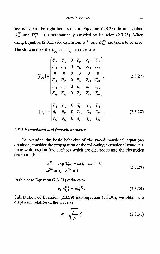
The structures of the cpq and e~jq matrices are
tcJ =
[«J =
s
/ — Cll
C21
0
C41
?S1
\C6\
"«ii g21
_?31
C12
C22
0
C42
C52
C62
g12
e12
e 32
0
0
0
0
0
0
0
0
0
C14
C24
0
C44
C54
c64
«14
e 2 4
g 34
ClS
C25
0
C45
C55
c65
% e 25
*35
^16
C26
0
S46
^56
C 6 6 ,
*16 "
e 26
« 3 « .
(2.3.27)
(2.3.28)
2.3.2 Extensional and face-shear waves
To examine the basic behavior of the two-dimensional equations obtained, consider the propagation of the following extensional wave in a plate with traction-free surfaces which are electroded and the electrodes are shorted:
M,(0) =exp/(£*i -cot),
^ » = 0 , ^ ( 1 ) =0.
In this case Equation (2.3.21) reduces to
/ l l " l , l l P"l •
i/f =0, (2.3.29)
(2.3.30)
Substitution of Equation (2.3.29) into Equation (2.3.30), we obtain the dispersion relation of the wave as
48 Mechanics of Piezoelectric Structures
Similarly, if we consider the propagation of the following wave:
,(°) ,(°) 0, u\' = exp/(^c, -cot),
0<°>=O, ^ ( 1 ) =0,
which is called a face-shear wave, Equation (2.3.21) reduces to
/66"2,11 — y"2 '
and the corresponding dispersion relation is
CO y66
(2.3.32)
(2.3.33)
(2.3.34)
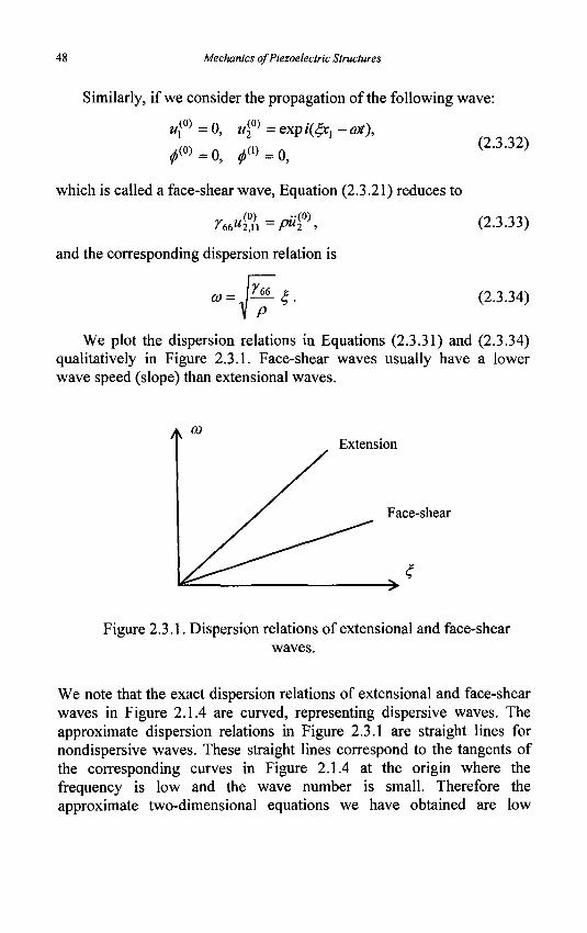
We plot the dispersion relations in Equations (2.3.31) and (2.3.34) qualitatively in Figure 2.3.1. Face-shear waves usually have a lower wave speed (slope) than extensional waves.
Extension
Face-shear
Figure 2.3.1. Dispersion relations of extensional and face-shear waves.
We note that the exact dispersion relations of extensional and face-shear waves in Figure 2.1.4 are curved, representing dispersive waves. The approximate dispersion relations in Figure 2.3.1 are straight lines for nondispersive waves. These straight lines correspond to the tangents of the corresponding curves in Figure 2.1.4 at the origin where the frequency is low and the wave number is small. Therefore the approximate two-dimensional equations we have obtained are low
Piezoelectric Plates 49
frequency, long wave approximations of the three-dimensional theory. They are valid when kh/ln « 1, or the wave length is much larger than the plate thickness. This gives a dynamic criterion of whether a plate is thin or not. It is relative to the wave length we are considering.
2.3.3 Equations for ceramic plates
We consider two cases of ceramic plates with thickness and in-plane poling.
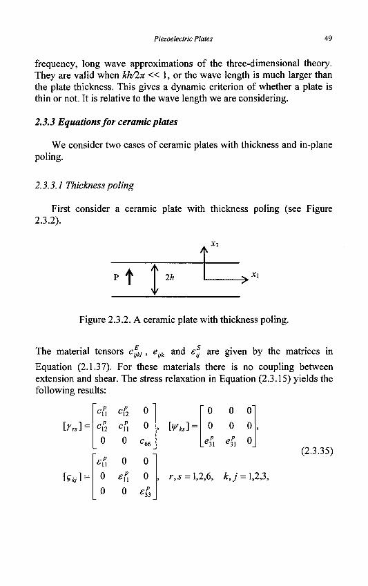
2.3.3.1 Thickness poling
First consider a ceramic plate with thickness poling (see Figure 2.3.2).
x3
t 2h X\
Figure 2.3.2. A ceramic plate with thickness poling.
The material tensors ciJkl, eijk and etj are given by the matrices in
Equation (2.1.37). For these materials there is no coupling between extension and shear. The stress relaxation in Equation (2.3.15) yields the following results:
[ / „ ] =
[?*•] =
-12
-11
0
0
0 0 c,
0
0
66
0
0 ~p ; 33
Wh\ =
0
0
e31
0
0
r,s = 1,2,6, £,./ = l,2,3,
(2.3.35)
50 Mechanics of Piezoelectric Structures
(2.3.36)
where
tfi =4 -(cf3)2/4 = *V[fan)2 "(4)2]> C12 = C 1 2 " f a n ) ' C 3 3 = _ 5 1 2 ' [ f a l l ) - ( 5 1 2 ) ]>
C66 = C66 = ^ ' , S ' 6 6 = fall ~CVl)'*->
e3\ - eZ\ ~ e 33 C 13 ' C33 = "31 ' f a l l + ^U ) '
-,P _ _S 2 I E b\\ ~ fcll ^ e 1 5 ' c44>
f 33 = ^33 + e33 ' C33 = f 33 ~~ ^"H^l.
c ^ , e? and £? are common notations for these plate material constants
[3] which clearly indicate that the constants are for a plate. The constitutive relations then take the following form:
T^=2h(c^+c{2u%-e^),
4°> = 2Kcf2uM + c1><°2) -e^Ef\ (2.3.37)
Df>=2he(xE?>,
DP-lKe&uW+e&EW), (2.3.38)
DV=-h3ent$>. (2.3.39)
Substitution of the above into the equations of motion and charge gives:
(2.3.40) rpum +c M(0) +(cp +c W0 ) +epcb{l)+ — F ( 0 ) - ou(0)
C l l " l l l + C"66M1,22 +VC12 +c66)u2,l\ + e3lr,l + „ , r \ ~ Hu\ >
2« VC12 +C66)"\,12 + C66U2,U + C l l " 2 , 2 2 + e3lV\2 + O/z _ 2 '
2«
2n
(2.3.41)
Piezoelectric Plates 51
The stress relaxation in Equation (2.3.23) yields:
P„]
v2x
0
0
0
0
[eiq} =
= 31
[*«] = 0
0
cf2 0
0 0
0 0
0 0
0 0
'31
0
0 FP
fc33
0
0
0
0
0
0 0 0 0
0 0 0 e 15
0 0
0
0
0
0 C44
0
0
0
0
0
0
C66 7
el5 0
0 0
0 0
, eu - £n - en dl5 /s 5 5 •
(2.3.42)
(2.3.43)
(2.3.44)
2.3.3.2 In-plane poling
Next consider a ceramic plate with in-plane poling along the JCI direction (see Figure 2.3.3).
2h
x3
Xi
Figure 2.3.3. A ceramic plate with in-plane poling.
In this case the material matrices can be obtained by tensor transformation or reordering rows and columns of the matrices in Equation (2.1.37) properly, with the result [9]:
52 Mechanics of Piezoelectric Structures
e 33
0
0
fc 6 33
Cl3
C 1 3
0
0
, 0
e31 e31
0 0
0 0
C13
Cll
C12
0
0
0
0
0
0
%
C12
c l l
0
0
0
0
0
«1S
0 0
0 0
0 0
^66 0
0 c44
0 0
0"
*1S
0 3
£ 3 3
0
0
o N
0
0
0
0
C 4 4 ,
5
0 0
£U 0
0 £l
(2.3.45)
where the elements of the matrices have the same meaning as those in Equation (2.1.37). For example, c33 is always the stiffness in the poling direction. The indices of the elements of the matrices in Equation (2.1.37) represent the positions of the elements in the matrices, but the indices of the elements of the matrices in Equation (2.1.45) do not. The stress relaxation in Equation (2.3.15) yields the following results:
[y»] =
[?*] =
Yu
Yn 0
£n 0
0
Yn
Yl2
0
0
*n 0
0
0
C44
0
0
^33
[Vfa] =
Vu 0
0
Yn 0
0
0
'15
r,s = 1,2,6, k,j = 1,2,3,
(2.3.46)
where
, £ \ 2 E ~E Y\\ ~ C 3 3 ~\C\i) ' C\\i Yl2~CU C12C13 /C11>
44' Yi2-C\\~\cn) ' c n » C 4 4 - C 4 4 - I / J
F 1 F F 1 F Yil = g33 _ g 31 C 13 ' C l l ' ^12 = g31 _ e 3 1 C 1 2 ' C l l '
?n = 4 + 4 ^ 11' £•11 = £• 11' ^33 _ £U + e i 5 ' C44-
(2.3.47)
Piezoelectric Plates 53
The constitutive relations then take the following form:
T^=2Kruu^+nA0}-^^0)l T2f =2h(ynu\y+y22u?l -yfuE™\ (2.3.48)
Ijf =2Mc44(<2)+*4°,))-%£n
Z)f =2M%(K,(°2) +«g )) + f n ^ 0 ) ] , (2.3.49)
D f ) = 2 ^ 3 3 ^ 0 ) ,
A ( , )=-f*3^a0). (2.3.50)
(2.3.51)
Substitution of the above into the equations of motion and charge gives:
ru«w +C44«S +(ri2 +C44)M^2)1
2n
Ol2 +C44)«U2 +C44«2°n + T ^ S
2«
^ l i r . n fci 1 ,22
+ VuKffi + e15«W + (<p12 + els )K<°>2 + -±-Dm = 0, (2.3.52) 2«
-*334i¥ " ^ +M-2C3Jm +7TT^(1) =0-
J3_
54 Mechanics of Piezoelectric Structures
The stress relaxation in Equation (2.3.23) yields:
F«] =
'11
-21
0
0
0
0
C12
C 22
0
0
0
0
0
0
0
0
0
0
0
0
0
C 66
0
0
0
0
0
0
C 44
0
0
0
0
0
0
Cu 44 J
(2.3.53)
[e,J =
eu en 0 0 0
0 0 0 0 0
0 0 0 0 e 15
;15 (2.3.54)
where
[%]: *11
0
C l l — C33 C13 ' C l l '
Ml
0
0
0 0 E 11
'12 — C13 C 12Pl3 ' C l l >
C 2 2 _ C 1 1 C 1 2 ' C 1 1 > e l l _ e 3 3 e 3 1 C 1 3 ' C l l '
e\2 ~ e3\ _ e 3 1 C 1 2 ' C l l > £U = £33 +e3l ' CW
(2.3.55)
(2.3.56)
2.3.4 Radial vibration of a circular ceramic disk
Consider a circular disk of a piezoelectric ceramic poled in the thickness direction positioned in a coordinate system as shown in Figure 2.3.4. The faces of the disk are traction-free and are completely coated with electrodes. A voltage Vexp(icof) is applied across the electrodes. We consider axi-symmetric radial vibrations [3].
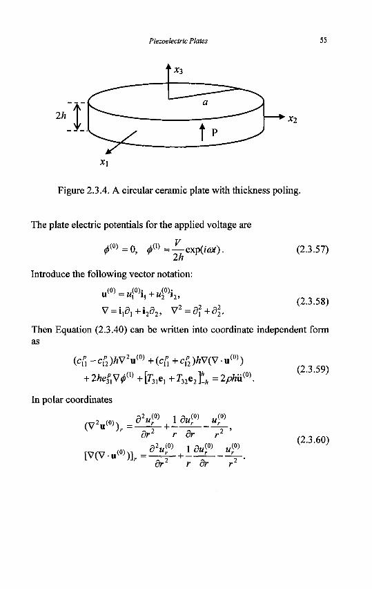
Piezoelectric Plates 55
2h x2
Figure 2.3.4. A circular ceramic plate with thickness poling.
The plate electric potentials for the applied voltage are
0(O>=O, <j>{V) =— exp(icot). 2h
Introduce the following vector notation:
V = i,S,+i2a2, V2=d2 + d22.
(2.3.57)
(2.3.58)
Then Equation (2.3.40) can be written into coordinate independent form as
(c/J -c,p2)W2u (0) +(c/; + c/2)/?V(V-u(0))
+ 2hep^<j>{X) + [r31e, + T32e2 ]th = 2phii(0).
In polar coordinates
(2.3.59)
( W ° > ) r = a2«<0) iew<°> ui0)
dr2 - + — r dr
[V(V-u(0))]r = d2«<0) 1 du™ ,«»
(2.3.60)
dr2 r dr
56 Mechanics of Piezoelectric Structures
Then for axi-symmetric motions Equation (2.3.59) becomes
+— = PU. (0)
dr2 r dr
The relevant resultants are
TP-VtcZsP+c&SW-eZEM)
= 2h(c(xiif} +c[2u(°) /r) + e&Vexp(ia*),
Df] = 2he& (u?) + 40) /r)-ef3V exp(/a*).
For steady state motions, Equation (2.3.61) reduces to
(2.3.61)
(2.3.62)
where
uf>„+^- +
2 = <0
1 ,(°) 0,
(ypf ,p\2
, (yp)=c^lp.
(2.3.63)
(2.3.64)
Equation (2.3.63) can be written as Bessel's equation of order one. For a solid disk, the motion at the origin is zero and the general solution is
u?)=BJx{Zr)extfi(ai), (2.3.65)
where J\ is the first kind Bessel function of the first order. Equation (2.3.65) is subject to the boundary condition
7-W =0, r = a,
hence Equation (2.3.66) requires that
C" dr + cp R^±---ep —
a 2« -12J
(2.3.66)
(2.3.67)
where, for convenience, the argument of the Bessel function is not written. From Equation (2.3.67) B can be expressed in terms of V as follows:
B = a -Potfa) c> 2h :
(2.3.68)
Piezoelectric Plates 57
where
dJx{x)
dx = • / „ ( * ) -
Jx{x) (2.3.69)
has been used and
• c 1 2 / c n , (2.3.70)
which may be interpreted as a planar Poisson's ratio, since the material is isotropic in a plane with a normal along x3. The total charge on the electrode at the bottom of the plate is given by
Q° = li-hD?)dA=2«\lTh
D(*)rdr- (2-3-71)
Substitution of Equation (2.3.65) into Equation (2.3.62)2 and then into Equation (2.3.71) yields
Qe = 2mPxaBJx (£a) - ne^Va212h.
Hence we obtain for the current that flows to the resonator
(2.3.72)
da dt
= 10J\
- M 2 2{kp
xYJx^a)
(l-ap)Jxtfa)-ZaJ0(Za)
£p3na2V
2h (2.3.73)
where
/M2
{K)2=^ Fp cp fc33cll
(2.3.74)
At mechanical resonance, the applied voltage can be zero, and from Equation (2.3.67),
dJ,
dr a (2.3.75)
Or, at the resonance frequency, the current goes to infinity. This condition is determined by setting the square bracketed factor in the denominator of Equation (2.3.68) equal to zero. The resulting equation is
58 Mechanics of Piezoelectric Structures
4aJ0(Za)=1_aPt ( 2 3 ? 6 )
which can be brought into the same form as (2.3.75). The antiresonance frequency results when the current goes to zero. The resulting equation is
^ i ^ l - g ' - W . ) 2 - (2-3-77)
The above results from plate equations are the same as the results in [3,9] obtained by directly making approximations in the three-dimensional equations.
2.4 First-Order Theory
In this section the first-order terms and equations are examined. A set of equations governing extension and flexure with shear deformations are obtained. These equations are probably the most widely used plate equations. The equations are specialized to the cases of ceramic and quartz plates.
2.4.1 Coupled extension, flexure and thickness-shear
By a first-order theory we mean a theory for coupled extensional
(uf\ a = 1, 2), flexural (uf^) and thickness-shear (u^) motions of a
plate. For the electrical behavior of the plate we are interested in what is
governed by ^(0) and </>m. The approximate displacement and potential
fields are
W(SM<0)+*3", (1 )+*32«, (2 ) ,
Although we are mainly interested in u\0) and u^, we have included a few additional displacement components in Equation (2.4.1). Among these additional displacements, u^ and uf) represent the thickness stretch or contraction accompanying extension and flexure due to Poisson's effect, and must be included. From Equation (2.2.6) it can be
seen that u^ together with u\2) and uf] contribute to symmetric
Piezoelectric Plates 59
thickness-shear deformations S^ and S*p, which may couple to the other first-order strains due to anisotropy and should be allowed. The two-dimensional plate equations we will obtain are for u^\ uf^ and
u^ only. Other displacements will be eliminated through stress relaxation procedures. Within the approximation in Equation (2.4.1), the strains and electric fields in Equations (2.2.5), (2.2.6), (2.2.8) and (2.2.9) become:
sf 0 )=M l<?, s<0)
" 4 ~ M3,2 + U2 '
£?>=-*?>,
EP=^f\
_„(0) - M 2 , 2 >
• " 2 , 2 »
£f =
p ( i ) •^2
e(0) _ M(D
- « ( 0 ) + » y ( 1 ) V(0) - M ( 0 > + M ( ° >
S3(1)=2Wf,
= iij),)+2ii1(2), S ^
-4°), E^=-^\
= -4>f, E?=0.
(2.4.2)
( 2.4.3)
(2.4.4)
(2.4.5)
Higher order strains S^ are neglected. From Equation (2.2.17)i, fory =
1, 2, 3 and n = 0, and fory =1 ,2 and n = 1, we obtain
TZ+Fr=2hpuf\ a,b = 1,2,
l%+F}°>=Zhpu?\ (2.4.6)
where we have truncated the right hand side by keeping the 5ooterm onty in the summation in the zero-order equations, and the Bu term only in the summation in the first-order equations. Equation (2.4.6)i is for extension, Equation (2.4.6)2 is for flexure, and Equation (2.4.6)3 is for thickness-shear. The electrostatic equations are the same as those in the zero-order theory in the previous section. We have, for an unelectroded plate:
60 Mechanics of Piezoelectric Structures
Dn+o^=o, DV-DM+D<»=O,
(2.4.7)
for a symmetrically electroded plate:
#w -hjm =V2(t),
for a plate electroded at the upper surface:
0(O)+/tf(I) =^(0,
-h(D% + Z)(0)) + Z>£ -Z><0) +Z>(1) =0,
and for a plate electroded at the lower surface:
A ( Z ) ( 0 ) + j D ( o ) ) + j D( i)_ j D(o ) + Z )( . )= 0 j
<P{0)-h</>m =V2(t).
(2.4.8)
(2.4.9)
(2.4.10)
For plate constitutive relations, we truncate Equation (2.2.12) by keeping the B0o and Bn terms only in the summation:
Tp=2h(cmSJ»-ekyEJ?),
D^^2HevkSf+svE^), (2.4.11)
1ij ~ ~ \Lijkl°kl ^kij^k h
(2.4.12)
0) where SJf* have been neglected. Since S^ contains u^l) and S
contains u'p and z/,(2), Equations (2.4.11) and (2.4.12) are not yet ready to be used for a theory of extension, flexure and thickness-shear. To obtain the proper constitutive relations we proceed as follows [13,17]. For the zero-order constitutive relations we take the following stress relaxation to be approximately true:
4 0 ) = 0 . (2.4.13)
Piezoelectric Plates 61
Then, in the manner of the derivation of Equations (2.3.23) through (2.3.26), we obtain the relaxed zero-order constitutive relations:
A(0)=2/Ke,rf+^f), (2.4.14)
where
Cijkl-Cijk! Cij33C33kl ' C3333>
ekij - ekij 'ek33C33ij ' C3333> (2.4.15)
£ij - Eij + emej33 ' C3333
Since we use a linear function x3u^ as an approximation for the fundamental thickness-shear mode in this first-order theory, which is approximate in dynamic problems where the fundamental thickness-shear displacement has a sinusoidal variation through the plate thickness, following [13,17], we introduce two shear correction factors Ki and K2 as follows. First a two-dimensional electric enthalpy can be defined based on Equation (2.4.14). Then we replace the following zero-order strains in the two-dimensional enthalpy function:
0 3 1 —> KlSn , S32 —> K2S32 .
T(0) P
(2.4.16)
This modifies cjjkl and eijk into ~c\jkl and e'yk in the zero-order
constitutive relations. Then Equation (2.4.14) takes the following form:
2h{c'nS^-e'kpE^),
The structures of the c'pq and ~e'iq matrices are
(2.4.17)
p»y-
'21
K-,C, 2 M 1
K,C 1*-51
V °61
'12
'22
KiC. 2M2
KiC. l c 5 2
'62
0
0
0
fC^Ci 2M4
IQ'sC-2^24
0 KxK2C5n
0 K2CM
K,C 11'25
K\K2Ci$
K\K\C55
K,C,
'16
'26
K-yC, 2M6
K\C l c 5 6
1C65 C 66 )
(2.4.18)
62 Mechanics of Piezoelectric Structures
F;I= «n e2i
h\
en
e22
e12
0
0
0
K2eU
K2eU
K2e14
K\e\5
K\e25
K\eii
«16
^26
*36_
(2.4.19)
The two correction factors should be determined by requiring the two fundamental thickness-shear resonant frequencies obtained from the two-dimensional plate equations to be equal to the corresponding exact frequencies predicted by the three-dimensional equations. With shear correction factors thus determined, the two-dimensional plate equations and the exact three-dimensional equations yield the same frequencies for a particular motion, i.e., the thickness-shear vibration of a plate in the two fundamental thickness-shear modes. This is particularly important to the analysis of piezoelectric devices operating with thickness-shear modes.
For the first-order constitutive relations, we set [13,17]
7;(1)=0, 9 = 3,4,5, (2.4.20)
Then, similar to the derivation of Equations (2.3.17) through (2.3.20), we obtain the relaxed first-order constitutive relations:
Tm =
D, 0)
2h3
2h3
:(») Oh {YnS\l> ~¥krEr\
(2.4.21)
m^ G^SJ"+^}U),
where
'CrvCvwCws' r>S~h^>V,
- e *H- c w c ™» V,W = 3,4,-
?kj = £kj + ekvcvwejw > . A * = 1>2,3.
/ rs rs *"rv~ VM*" ws '
Vks = eks - ekwCw\Cvs , V > W = 3 A5 '
- 1 .
(2.4.22)
Piezoelectric Plates 63
In summary, in the case of an unelectroded plate, we have obtained
r ( 0 ) 1ab,a
r ( 0 ) Ia3,a
y( l ) 1ab,a
fl(0) a,a
Dm a,a
+ ^ ( 0 )
+ /f>
r ( 0 )
+ J D ( 0 )
-Z>< 0 )
= 1hpuf,
= 2hpuf\
* 3
= 0,
+ JD(1)=0,
a,b =
-pa?..
U
i (2.4.23)
7f =2/*c^-^£f), zf>=2/<erf+^f),
sf*
sf s, (1) = £<°>
£, ( 1 )
DV=^isS<?+<;vEf),
_ M(0) o(0) _ (0) — « j j , 0 2
— "2,2 »
- w ( 0 ) + w (1) <7(0) - M (0) + jy ( I ) 9 ( 0 )
_ M(l) c(l) _ ,.(1) c(l) _ , .0) . ,.(1) ~ "l,l ' " 2 — " 2 , 2 ' ° 6 — "1,2 + " 2 , 1 '
= -<*f, ^ 0 ) = - ^ , Ef =-/*>, = - ^ , £ « = ^ « , £ 3
0 ) =0.
= 1,2,6,
- M ( 0 ) + M ( 0 ) _ " l , 2 + " 2 , 1
( 2.4.24)
(2.4.25)
With successive substitutions from Equations (2.4.24) and (2.4.25),
Equations (2.4.23) can be written as seven equations for wf), u?, ^(0)
and <j>m. At the boundary of a plate with an in-plane unit exterior normal
n and an in-plane unit tangent s (see Figure 2.2.1), we may prescribe
7 T or „<»>, T™ or u?\ T™ or uf\
& or „ « , r « or „ « , (2.4.26)
Z)<0) or <*(0), / ) « or ^ > .
64 Mechanics of Piezoelectric Structures
When electrodes are present the differential equations are fewer, and so are the boundary conditions. We note that Equations (2.4.23) through (2.4.25) do not contain Sf* and S® (w = 3, 4, 5), and the related displacement components u^ and wp^. These strain and displacements can be determined approximately from the stress relaxation conditions in Equations (2.4.13) and (2.4.20) once the solution to Equation (2.4.23) through (2.4.25) has been obtained.
2.4.2 Flexural and thickness-shear waves
To examine the basic behavior of the equations obtained, we study the special case of an isotropic, elastic plate for which
[*«]=
cu C12
c12
0
0
, 0
cn=X +
c12
<hi
C\2
0
0
0
2M, C\2 ~ "••>
C44 = ( C 1 1 —
[e, p]=
cu)/2
o,
cu
cu
0
0
0
0
0
0
C44
0
0
0
0
0
0
C44
0
(T 0
0
0
0
c 44y (2.4.27)
where X and fi are Lame constants. In this case extension is not coupled
to flexure and thickness-shear. Consider coupled flexure uf\xltt) and
thickness-shear in the JCI direction w,(1) (xl, t) . The relevant equations
reduce to
(0) .0)1 Du^-2hMK\u^+u\l>) 2h3
-pu\ (i)
(2.4.28)
Piezoelectric Plates 65
where [13]
D= 2kE2 , K = KX=K2=-^=. (2.4.29)
3(l-v2) Vl2
D is the bending stiffness of the plate. E is Young's modulus, v is Poisson's ratio. We look for simple wave solutions
M,(1) = A, exp i(£x, - cat), 1 x v ^ (2.4.30)
«30) = A3 exp /(<fptj - cot),
where ,4] and A3 are constants. Substitution of Equation (2.4.30) into Equation (2.4.28) results in two linear equations for A\ and A3. For nontrivial solutions the determinant of the coefficient matrix of the linear equations has to vanish. This yields the following equation that determines the dispersion relations for coupled flexural and thickness-shear waves:
where
x = col
-4h, n2
Ah2
n =
P
COl (!)„
?u =
)'
8
K2
1 1 - V
3Q4 -3 f i 2 -3Q 2 r u X 2 - X2a2 + yuX4 = 0, (2.4.31)
(2.4.32)
X is a dimensionless wave number. £1 is a dimensionless frequency, normalized by the exact fundamental thickness-shear frequency co*,. There are two branches of dispersion relations. For short waves with a small X, the asymptotic expressions of the two dispersion relations are
Q2^hLX\ flexure, (2.4.33)
and
Q2 ~\ + {yn+-)X2, thickness-shear. (2.4.34)
The two dispersion curves are qualitatively shown in Figure 2.4.1. With the correction factor the plate equations predict the exact cutoff frequency at Q. = 1.
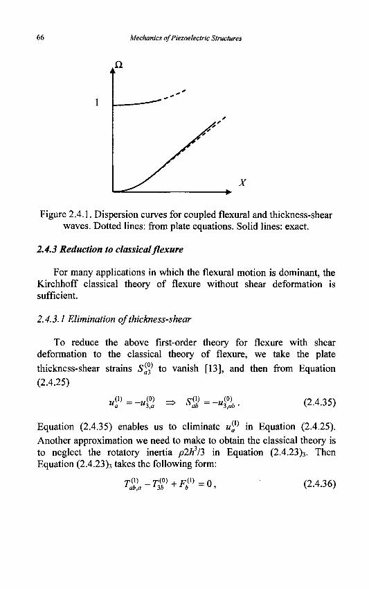
Mechanics of Piezoelectric Structures
X
Figure 2.4.1. Dispersion curves for coupled flexural and thickness-shear waves. Dotted lines: from plate equations. Solid lines: exact.
2.4.3 Reduction to classical flexure
For many applications in which the flexural motion is dominant, the Kirchhoff classical theory of flexure without shear deformation is sufficient.
2.4.3.1 Elimination of thickness-shear
To reduce the above first-order theory for flexure with shear deformation to the classical theory of flexure, we take the plate
thickness-shear strains S$ to vanish [13], and then from Equation (2.4.25)
, ( i) -u
(0) 3,a
e( l ) ^ab -u
(0) 3,ab (2.4.35)
Equation (2.4.35) enables us to eliminate u® in Equation (2.4.25). Another approximation we need to make to obtain the classical theory is to neglect the rotatory inertia p2h3/3 in Equation (2.4.23)3. Then Equation (2.4.23)3 takes the following form:
1ab,a 13b ^ r b 0. (2.4.36)
Piezoelectric Plates 67
from which we can solve for TJb0) and substitute the result into Equation
(2.4.23)2 to obtain the equation for classical flexure
r « « + F « + / ^ > = 2 ^ f > . (2.4.37)
In summary, the equations for extension and classical flexure are:
TZ+F?>=lhpu¥\ a,b = \,2,
T$a+Fr=2hpu?\
<>+£(0)=o,
D?1-DP+DV=O,
(2.4.38)
T^=2h(c'rsS^-eiE^), r,s = 1,2,6,
T^=T^.+Fbm, (2.4.39)
A0)=^-(^I(,)+^y)x
C(0) _ ,.(0) o(0) _ (0) v(0) _ (0) (0) ° 1 — "1,1 > ° 2 — " 2 , 2 > " 6 — "1,2 + " 2 , 1 »
e(l) _ _„(0)
£,(0)=^j0), E^=-^\ E^=-^l\
EV=-$\ E?=-4$\ EV=0.
With successive substitutions from Equations (2.4.39) and (2.4.40), Equations (2.4.38) can be written as five equations for u$°\ ^(0) and
<f>^'. At the boundary of a plate with an in-plane unit exterior normal n
and an in-plane unit tangent s (see Figure 2.2.1), we may prescribe
(2.4.40)
68 Mechanics of Piezoelectric Structures
7 T or „<°>, 7-W or «<»>, (2 4 411
•ln3 + i m , i ° r "3 > i nn ° r «3,« •
2.4.3.2 Dispersion curves offlexural waves
The above procedure for reduction to classical flexure is more readily seen in the special case of isotropic materials. We begin with the following equations from Equation (2.4.28) for coupled flexure and thickness-shear:
2hfiK2 (4% + wft) = 2hpuf),
2 / 3 (2.4.42) Du^-2hMK2(u^+u^)^— pu?\
First we set the rotatory inertia to zero in (2.4.42)2. This results in
Dux% - 2hnK1 (ufx + uxm ) = 0 . (2.4.43)
The elimination of 2h(/ju^x + uxm) from Equations (2.4.43) and
(2.4.42), yields
Duj$u = 2hpuf). (2.4.44)
Next we set the plate shear strain to zero
uf}+u\l)=0, (2.4.45)
with which we can express w,(1> in terms of uf^ in Equation (2.4.44)
-Duf}m=2hpuf>, (2.4.46)
which is the well-known equation for classical flexure. In Equation (2.4.46), letting
uf)=Gapi(&x-aX), (2.4.47)
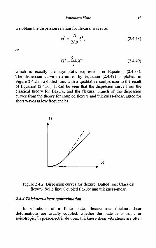
Piezoelectric Plates 69
we obtain the dispersion relation for flexural waves as
,-?• D P*
2hp (2.4.48)
or
Q 2 Tu X* (2.4.49)
which is exactly the asymptotic expression in Equation (2.4.33). The dispersion curve determined by Equation (2.4.49) is plotted in Figure 2.4.2 in a dotted line, with a qualitative comparison to the result of Equation (2.4.31). It can be seen that the dispersion curve from the classical theory for flexure, and the flexural branch of the dispersion curves from the theory for coupled flexure and thickness-shear, agree for short waves at low frequencies.
Q
X
Figure 2.4.2. Dispersion curves for flexure. Dotted line: Classical flexure. Solid line: Coupled flexure and thickness-shear.
2.4.4 Thickness-shear approximation
In vibrations of a finite plate, flexure and thickness-shear deformations are usually coupled, whether the plate is isotropic or anisotropic. In piezoelectric devices, thickness-shear vibrations are often
70 Mechanics of Piezoelectric Structures
used as the operating modes. These modes are dominated by thickness-shear deformations, with a small coupling to flexure. There is a procedure for eliminating the weak coupling to flexure from the equations for coupled flexure and thickness-shear to obtain equations for the dominating thickness-shear waves only. This procedure is called the thickness-shear approximation [27], and is particularly useful in analyzing piezoelectric devices. Thickness-shear approximation was introduced in the analysis of quartz thickness-shear piezoelectric devices [27]. The procedure can be well explained in the case of an isotropic plate, which will be presented below. We begin with the equations for coupled flexure and thickness-shear (Equation (2.4.28))
2hnK2 (B<5» + « $ ) = Ihpuf,
2 / 3 (2.4.50) Dux% -2hMK2(4°? +uV) = —piiW.
Let «!(1) = Ax exp/(£c, - cot),
M30) - ^3 eXP K&\ - <*#)•
Substituting Equation (2.4.51) into Equation (2.4.50)], we obtain
(2.4.51)
HK2{-A^2 + Axi$) = -poj2A3. (2.4.52)
For long waves we drop the term quadratic in t,. For frequencies close to the lowest thickness-shear frequency fife we set
Ah p
in Equation (2.4.52). Then Equation (2.4.52) becomes
A3=~4%, (2-4-54)
which is equivalent to the differential relation
"f =-y«S). (2-4-55)
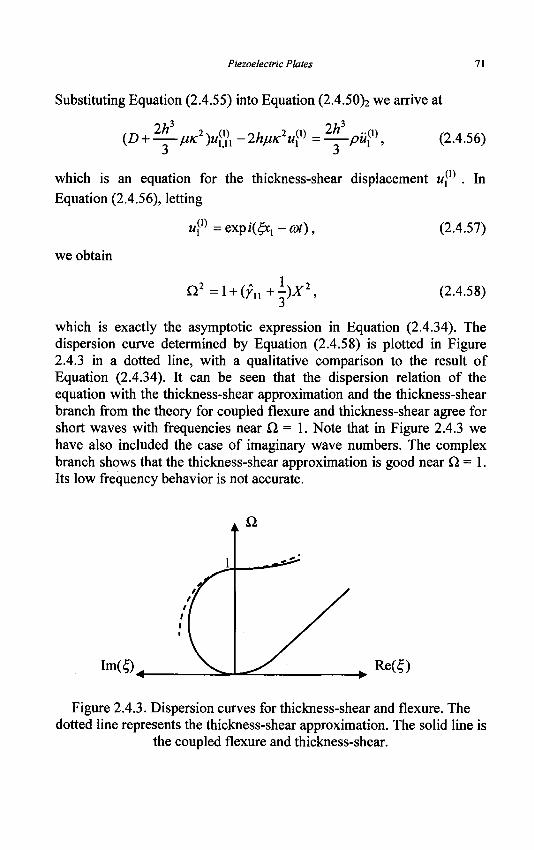
Piezoelectric Plates 71
Substituting Equation (2.4.55) into Equation (2.4.50)2 we arrive at
2k (D + HKL X n - 2h/iKzu\ (i) -2„0) - 2h3
-P«i (i) (2.4.56)
which is an equation for the thickness-shear displacement w,(1) . In Equation (2.4.56), letting
u[x) = exp /(£:, - cot), (2.4.57)
we obtain
G.2=\ + (9n+hx2, (2.4.58)
which is exactly the asymptotic expression in Equation (2.4.34). The dispersion curve determined by Equation (2.4.58) is plotted in Figure 2.4.3 in a dotted line, with a qualitative comparison to the result of Equation (2.4.34). It can be seen that the dispersion relation of the equation with the thickness-shear approximation and the thickness-shear branch from the theory for coupled flexure and thickness-shear agree for short waves with frequencies near £ 2 = 1 . Note that in Figure 2.4.3 we have also included the case of imaginary wave numbers. The complex branch shows that the thickness-shear approximation is good near £2=1. Its low frequency behavior is not accurate.
I m ( ^ Re(£)
Figure 2.4.3. Dispersion curves for thickness-shear and flexure. The dotted line represents the thickness-shear approximation. The solid line is
the coupled flexure and thickness-shear.
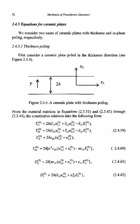
72 Mechanics of Piezoelectric Structures
2.4.5 Equations for ceramic plates
We consider two cases of ceramic plates with thickness and in-plane poling, respectively.
2.4.5.1 Thickness poling
First consider a ceramic plate poled in the thickness direction (see Figure 2.4.4).
X3
f 2h * i
Figure 2.4.4. A ceramic plate with thickness poling.
From the material matrices in Equations (2.3.35) and (2.3.42) through (2.3.44), the constitutive relations take the following form:
T<?> = 2h{cnu™+cnu™-e^),
'22 = 2"(C12M1,1 +C11M2,2
71?)=2*c66(«S>+ii<5X
T™ =2*(c12n<°> + c n t $ - e r f * ) , (2.4.59)
.(0) 0 > ) . , f d h rWi r ^ = 2 M ^ 4 4 « j + C ) - ^ 1 5 ^ r ] ( 2.4.60)
(0) j . „ 0 ) i r(Oi Dr=2/ lK 5«+^)+^^r] (2.4.61)
DW=2h(e31u%+e^), (2.4.62)
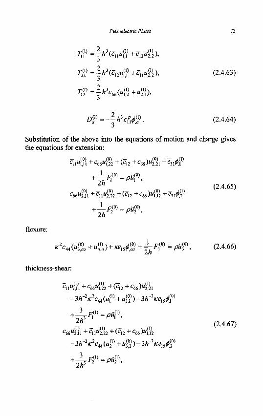
Piezoelectric Plates 73
r1?>=|A3(cI1«g>+c12iigx
4° =\h\cX24J + cni/$), (2.4.63)
^=f^66(^+^),
Substitution of the above into the equations of motion and charge gives the equations for extension:
C11M1,11 + C66M1,22 + ( C 1 2 + C 6 6 ) M 2 , 2 1 + e 31^ , l
in
+ J_/r(0)-/7w(0) + r2 - pu2 ,
in
flexure:
thickness-shear:
C11M1,11 + C 6 6 M 1 , 2 2 + ( C 1 2 + C 6 6 ) M 2 , 2 1
- 3/rVc44 (Ml(1) + «3
(y) - 3h-2ice^f)
C66M2,11 + C 1 1 M 2 , 2 2 + ( C 1 2 + C 6 6 ) M 1 , 1 2
- 3/f Vc 4 4 {uf + i/g) - 3h"2Kexs(t>[
+ — Fm-rnim
,(»)
(2.4.65)
K2C<M),a +U2>^5*S + i F 3 ( 0 ) = Pfi<°>, (2.4.66) 2«
(2.4.67)
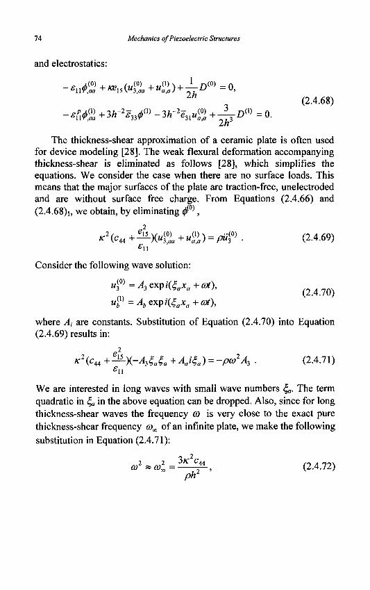
74 Mechanics of Piezoelectric Structures
and electrostatics:
(2.4.68) -s?xC +3h~%^ -3h-*e3lu% + - L i ) 0 ) = 0 .
The thickness-shear approximation of a ceramic plate is often used for device modeling [28]. The weak flexural deformation accompanying thickness-shear is eliminated as follows [28], which simplifies the equations. We consider the case when there are no surface loads. This means that the major surfaces of the plate are traction-free, unelectroded and are without surface free charge. From Equations (2.4.66) and (2.4.68)i, we obtain, by eliminating 0(o),
* 2 ( c „ + ^ X « 3 ^ + « . 0 i ) = / * j 0 ) . (2-4.69)
Consider the following wave solution:
"i0) = A, expi(£nx„ + cot), 3 3 F V*„ a h (2.4.70)
«*° =AGXPi(^axa+cot),
where At are constants. Substitution of Equation (2.4.70) into Equation (2.4.69) results in:
K2{c„+^X-MaSa+Aai$a) = -p<o1A3 . (2.4.71)
We are interested in long waves with small wave numbers £,. The term quadratic in £, in the above equation can be dropped. Also, since for long thickness-shear waves the frequency CO is very close to the exact pure thickness-shear frequency cox of an infinite plate, we make the following substitution in Equation (2.4.71):
co^colJj^L, (2.4.72) ph
Piezoelectric Plates 75
where <o„ is determined from Equation (2.4.67)i by dropping all x\ and x2 dependence as well as the surface load. The approximate version of Equation (2.4.71) is then
A = -4-0 + -^-MaK, (2-4-73) 3 cAAsn
which is equivalent to the differential relation
« 3 W = - y 0 + *,25)«2, (2A74)
where we have denoted
/ f c , 25 =-^ - . (2.4.75) C44fll
Substituting Equation (2.4.74) into Equations (2.4.67) and (2.4.68)b
neglecting the third derivatives of uam under the long wave
approximation, we obtain the following equations under the thickness-shear approximation:
ClVftl +C66"U2 +C,>2!l2 -Pat?? -^h^KB^ = fM®,
C(i6H2% + cnu%2 + cnu^}2 - pulu® - 3h-2KB^20) = puf, (2.4.76)
-*„#2+«„«« =0, where
Cll — C l l + K " C44 (1 + 15 )' (2.4.77) C12 _ C 1 2 + C66 +K c44 0 + *15/'
Under the thickness-shear approximation, we approximately have
D^=2KKB15U^+SUE^). { -
2.4.5.2 In-plane poling
Next consider the case of a ceramic plate with in-plane poling in the JCI direction (see Figure 2.4.5).
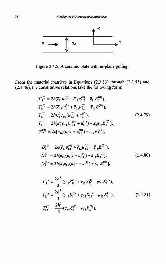
Mechanics of Piezoelectric Structures
Xi
2/i * i
Figure 2.4.5. A ceramic plate with in-plane poling.
From the material matrices in Equations (2.3.53) through (2.3.55) and (2.3.46), the constitutive relations take the following form:
T^=2h(cuu$+c22u?l-enE^),
T2f=2hK22c66(u%+u?\
T^=2h[K?c<M°l +u?)-Kle15E?)],
r/2°)^2Mc44(M<°2)+^)-e15JBf],
(2.4.79)
A(0) =2h(euuW + el2u^+euE^),
Z)f =2h[exMQl^J) + snEf\
Df=2h[KleX5{ufl+uV) + snE^l
(2.4.80)
(2.4.81)
Piezoelectric Plates 77
2h3
DP^tfiuSV+enEJP), (2.4.82)
nd) _ M_/- Em
UZ - - ^ 3 3 ^ 3 •
Substitution of the above into the equations of motion and charge gives the equations of extension:
C11M1,11 +C44M1,22 + ( C 1 2 +C44)M2,21
2h
(C12 +" c44 )M1,12 +C44M2,11 +C22M2,22
In
flexure:
thickness-shear:
(2.4.83)
K\ c44 (M3,ll + Ml,l ) + K2 C66 (M3,22 + M2,2 )
1 (2.4.84)
In
WW +C44«1% + ( T l 2 +C44)"2! 21 + ^ 1 1 ^ U
+ ej5$> -3r2[/r,2c44(<1) + M l
( V ^ 1 5 / 1 ) ]
+ -l-FU=pu?\ (2.4.85) in
(Tl2 + C 4 4 ) " U 2 +C44"2!ll + ^ 2 2 ^ 2 2 + (g15 + ^ 1 2 ¥,12
- 3 r V 22 c 6 6 « 2 ) + M f ) + - ^ ^ = ^ ,
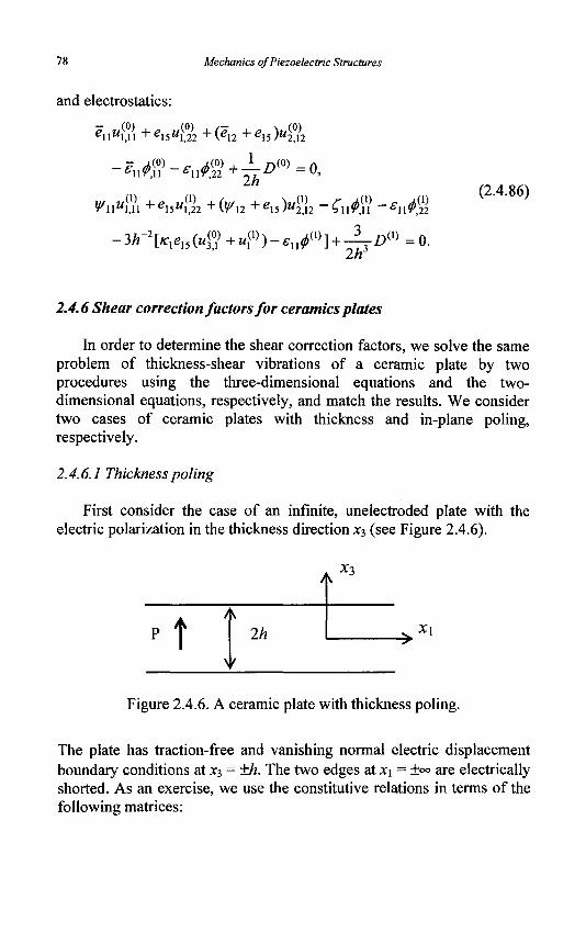
78 Mechanics of Piezoelectric Structures
and electrostatics:
(0) «ll«l,li +e15"l,22 +(£12 + e i s M . 1 2
1 F s(0)
-F dm + — nm
,(') _•_„ „(•) ±(tl, _•_„ \„o) _r /*(!)_£• Am y/uu\>x +ex%u\{2 +(y/n + eX5)u2i>n -Cu^ii - * i i $ 2
- 3 ^ [ / r i e , 5 « / + t t W ) - e i I ^ ] + Itf
(2.4.86)
2.4.6 Shear correction factors for ceramics plates
In order to determine the shear correction factors, we solve the same problem of thickness-shear vibrations of a ceramic plate by two procedures using the three-dimensional equations and the two-dimensional equations, respectively, and match the results. We consider two cases of ceramic plates with thickness and in-plane poling, respectively.
2.4.6.1 Thickness poling
First consider the case of an infinite, unelectroded plate with the electric polarization in the thickness direction x3 (see Figure 2.4.6).
x3
t Ih xi
Figure 2.4.6. A ceramic plate with thickness poling.
The plate has traction-free and vanishing normal electric displacement boundary conditions at JC3 = ±h. The two edges at x\ = +°° are electrically shorted. As an exercise, we use the constitutive relations in terms of the following matrices:

Piezoelectric Plates 79
'12 "13
'12 11 J13
M3 J13 '33
0 0
0 0
0 0
0 ^
0
0
44 0 0 0 *
0 0 0 0
0 0 0 0
0 0
f 0 0
0 0
V^31 ^31
0
0 £/,
' 33
0 </15 (fi 0 0
5 44
r„r
5 66 7
0 0
0 0
0 0 £ 33
(2.4.87)
where *66 = 1{s\\-sn )• We look for solutions in the following form:
Ux = Wj (X3 , 0 , M2 = M 3 = 0, ^ = 0 , (2.4.88)
which lead to
i J i — U i — I J T
^ = £ 2 = £ 3 = 0 ,
S4=S6=0, S5 *1,3>
T^T2=T3^T4=T6=0, T5=—uh 3 ' (2.4.89) 3 44
£>!=—w1 3 , Z>2=JD3=0.
The equation and boundary conditions to be satisfied are
1 -tt,33 = pux, •h<x3 <h,
3 44
r 3 , = 1
(2.4.90) M, 3 = 0, X3 = ±/z,
344
which allow the following simple solution for the lowest thickness-shear mode
• mT, ,• - 2 7 It
w,=sin exp(jfttf), co =coK=—z 2c 4hlpsu
(2.4.91)
80 Mechanics of Piezoelectric Structures
Note that the solution is not pure elastic because of the following nontrivial electric displacement component:
D, = ^S5 = ^LiLcos^LexpO-fl*), (2.4.92) ^44 ^44 ^C ^
which is responsible for the current flowing through the shorted edges at x\ = ±°°. To determine the correction factor K, we also consider the above thickness-shear mode from the plate theory. From Equation (2.4.67)i we have, with 3, = d2 = 0, (jf0) = 0, and <j>m = 0,
h2s ,(l) _ ~;( l ) pii\l>, (2.4.93)
44
which implies that
ft>2= 3*~ . (2.4.94) ph s 44
Comparing the frequencies in Equations (2.4.91) and (2.4.94), we determine the correction factor as
K2= — . (2.4.95) 12
The above solution is for the case when the two edges of the plate at JCJ = ±oo are shorted. If the two ends of the plate are open (which implies that Di(0) vanishes but E\-0) survives in the plate theory), then from the plate equations we have
a £ » 2 *\ . 2 , » * . 2 5 = - ^ - . (2-4-96)
2.4.6.2 In-plane poling
Next consider the case of a ceramic plate with in-plane poling in the xi direction (see Figure 2.4.7). The plate is unelectroded at its major surfaces.
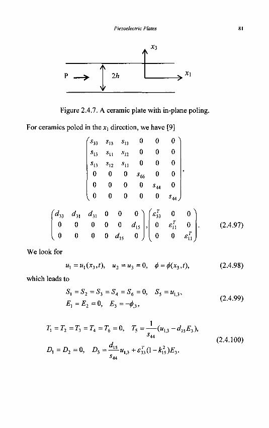
Piezoelectric Plates
*3
2h x\
Figure 2.4.7. A ceramic plate with in-plane poling.
For ceramics poled in the x\ direction, we have [9]
'33
'13
'13
0
0
0
5 1 2
0
0
0
J12
*11
0
0
0
0
0
0
0
0
0
0
0
0
S44
0
0
0
0
0
S44 7
(d. 33
0
0
"31
0 "31
0
0
0
0
0
0
0
dl5
*15
6 33
0
0
0
0 (2.4.97)
We look for
ux=ux{x3,t), u2=u3=0, $ = 0(x3,t),
which leads to
5", - iS"2 - S3
Ex=E2=0, - 0 . 3 >
(2.4.98)
(2.4.99)
T\ = T2 = T3 = T4 = ^6 = °> ^5 = ("1,3 - ^ 1 5 ^ 3 )> '44
Dx=D2=0, I>3 = — uX3 + eT33 (1 - kX5 )E3.
'44
(2.4.100)
82 Mechanics of Piezoelectric Structures
The equation and boundary conditions to be satisfied are
5—Mi33=P"i> -h<x,<h,
(2.4.101)
^31 = T~U\ 3 = 0 ' Xi= ± n ,
5 4 4 ( l -^ 25 ) U
which allow the following simple solution for the lowest thickness-shear mode
. I O C , . . . w, =sin—-exp(*6#),
2h 2 (2.4.102)
2 2 11
4^44(l-4) The corresponding plate solution can be found from Equations (2.4.85)i and (2.4.86)2 as
3K-2
co2 - — ! —. (2.4.103) ph2s44(l-k?5)
Comparing Equations (2.4.102) and (2.4.103) we obtain
If the plate is electroded at x^ = ±h and the electrodes are shorted, from the plate equations we have
n 2
< » > — — - . (2.4.105) 4ph s 44
2.4.7 Thickness-shear vibration of an inhomogeneous ceramic plate
As an application of the equations obtained, we analyze thickness-shear vibrations of an inhomogeneous ceramic plate with thickness poling (see Figure 2.4.8) [25]. The thick lines represent electrodes. The analysis is also valid for a plate of 6mm crystals with the six-fold axis along the plate thickness. This structure has various applications in piezoelectric devices operating with thickness-shear modes. When a »
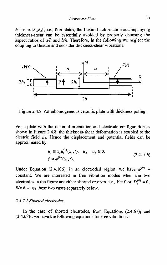
Piezoelectric Plates 83
h = max{h\,h2}, i.e., thin plates, the flexural deformation accompanying thickness-shear can be essentially avoided by properly choosing the aspect ratios of ct/h and b/h. Therefore, in the following we neglect the coupling to flexure and consider thickness-shear vibrations.
-v{t).
?/?•, + Arii t
a V y
Pf 2/?, < '
vX3
a
V
i i
s
V{t)
/ • T
X\
*
y<r 2b
Figure 2.4.8. An inhomogeneous ceramic plate with thickness poling.
For a plate with the material orientation and electrode configuration as shown in Figure 2.4.8, the thickness-shear deformation is coupled to the electric field E\. Hence the displacement and potential fields can be approximated by
Wj = x^u'p {xx,t\ u2 = w3 = 0, (2.4.106)
Under Equation (2.4.106), in an electroded region, we have ^(0) = constant. We are interested in free vibration modes when the two electrodes in the figure are either shorted or open, i.e., V= 0 or .D,(0) = 0 . We discuss these two cases separately below.
2.4.7.1 Shorted electrodes
In the case of shorted electrodes, from Equations (2.4.67)i and (2.4.68)i, we have the following equations for free vibrations:
84 Mechanics of Piezoelectric Structures
ciXft - 3VVc4 4"i ( 1 ) - 3V 2 « 1 5 ^ 0 ) = pw,(1), | x, |< a,
- su&fi + KB15U® - 0 , \xx \< a,
cuu\x}\ -3h22K2cHu{l) = pu\x), a <| xx \<b,
M,(,) (±a" ) = w,(1) (+a+), (2.4.107)
«1(i)(±a-) = «1
(i)(±a+),
^ ( 0 ) ( ± f l - ) = 0,
u?\±b) = 0,
where K2 = n2 111. Note that Equation (2.4.107)5 is of an approximate nature. In Equation (2.4.107) we directly neglected the coupling to flexure and did not use the thickness-shear approximation to eliminate flexure. Consider time-harmonic motions with a frequency co. Then Equations (2.4.107)i>3 can be written as
?„«,<?, + p(co2 - co2 )Ml(,) - 3V2**W,(,0) =0, I x, |< a,
cuu^ + p(co2 - a>\ )w,(1) =0, a<\ xx |< b, (2.4.108)
where
r2 _ 3K c44 _ K C44 „ 2 _ 3 y C44 ?T ^44 /-^ ,i i r . 0 \
^ = ^ J 7 " - 7 I I T ' ^ - - ^ — - - 7 2 - (2.4.109) 2 _ -»v ^44 _ " ^44 2 _ - , / v M 4 _ " M 4
are the pure thickness-shear frequencies of a plate of thickness 2h\ or 2/Z2 when there is no piezoelectric stiffening due to E\. Equation (2.4.107)2 can be integrated to give
^ ( 0 ) = ^ i L t t ( i ) + C i > \Xx\<a, (2.4.110)
where C\ is an integration constant. Substitution of Equation (2.4.110) into Equation (2.4.108)i yields
cuiift + p{co2 -c5x2)u^ - ^ - C , =0, I xx |< a , (2.4.111)
Piezoelectric Plates 85
where
2
ax2 = a] (1 + kx\), /fc2
5 = — i 2 - . (2.4.112) £11C44
^ is the pure thickness-shear frequency of a plate of thickness 2h\ when there is piezoelectric stiffening due to E\. The general solutions to Equation (2.4.111) and Equation (2.4.108)2 are
wP = C3 cosh axx + C4 sinh axx+yCx, \xx\< a,
uxm = C5 cosfixx + C6 sin flxx, a<xx< b, (2.4.113)
wP = C7 cos /3xx + Cg sin /2c,, - 6 < JCJ < -a ,
where C3 through C6 are integration constants, and
oc — ,
p2=P(fi?_-*bt ( 2 4 1 1 4 )
pia)2-^)^'
With Equation (2.4.113)i, Equation (2.4.110) can be integrated once more to yield
( 1 i A
(2.4.115) KB t 1 I
^(0) _ — n Q —sinh axx + C4 —coshaxx + yCxx £xx \ a a
+ Cxxx +C2, \xx \<a,
where C2 is another integration constant. Substitution of Equations (2.4.113) and (2.4.115) into the boundary and continuity conditions in Equation (2.4.107) results in a system of homogeneous equations for C\ through C6. For nontrivial solutions the determinant of the coefficient matrix has to vanish, which determines the eigenvalues or resonant frequencies. Mode shapes are determined by the eigenvectors. Because of the symmetry in Figure 2.4.8, the modes can be separated into two
86 Mechanics of Piezoelectric Structures
groups. One is called symmetric and the other anti-symmetric in xx. In applications the symmetric modes when M,(1) is an even function of JCJ are useful, especially the lowest one. For these modes we let
C2 — C4 — U, C7 — C5 , Cg -c, (2.4.116)
Then from the continuity and boundary conditions at a and b, we obtain the following equations for C\, C3, C5 and C6:
C3 cosh aa + yCx =C5 cos /3a + C6 sin /3a,
C3a sinh oca = -C5/3 sin Pa + C6/? cos/far,
KB 15 C3 —sinhaa + a I + Cxa = 0, (2.4.117)
C5cos/% + C6sin/% = 0.
The frequency equation is
7xe15 tanhaa > ^ 1 + yivu
aas, (2.4.118)
• aa tan fl(b - a)tanh aa 1 + YKBli
MI y = 0.
First consider a plate of uniform thickness ( hx =h2). In this case
cox > a>2. As a numerical example, we consider the case of hx = h2 = 1 mm, a = 22 mm, b = 30 mm, and the electrodes are shorted. Cadmium Sulfide (CdS) is used in the calculation. The material constants are given
in Appendix 2. For a>2 < a < o5x , the modes are hyperbolic (or exponential) in the unelectroded region and sinusoidal in the electroded region. The first mode of ux
m is plotted in Figure 2.4.9. The vibration is essentially in the electroded region; once it enters the unelectroded region it decays rapidly. The cause of this type of behavior is that the piezoelectric stiffening effect in the unelectroded central region makes
a>x >a>2. The corresponding ^(0) is shown in Figure 2.4.10.
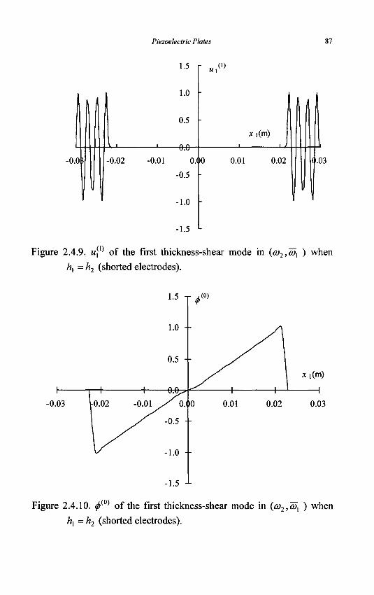
Piezoelectric Plates 87
II 0.0 (
I
ll . 1
-0.02
I
-0.01
1.5
1.0
0.5
V.K)
0.1
-0.5
-1.0
-1.5
r « . ( , )
X
i
)0 0.01
1 i(m)
0.02
1
ll i
(|.03
If Figure 2.4.9. w,(1) of the first thickness-shear mode in (co2,a)x ) when
hx = h2 (shorted electrodes).
-0.03
•1.5 J-
0.03
Figure 2.4.10. ^(0) of the first thickness-shear mode in {co2,cox ) when
hx = h2 (shorted electrodes).
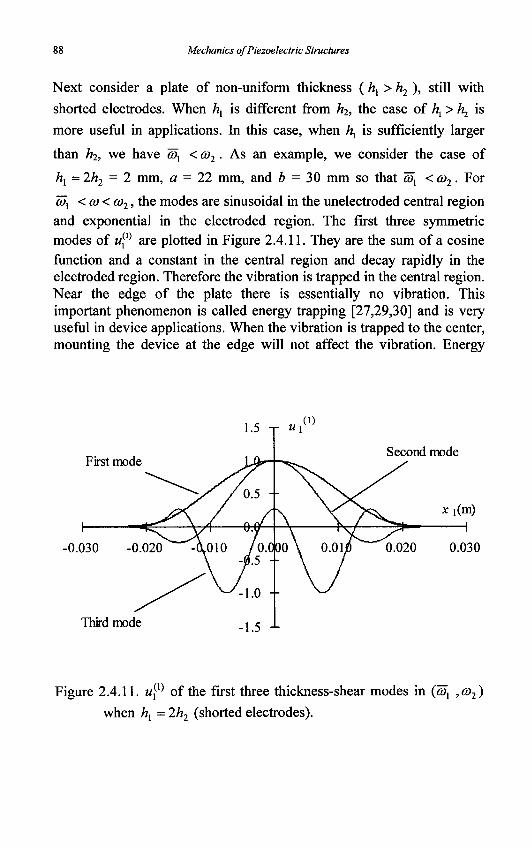
gg Mechanics of Piezoelectric Structures
Next consider a plate of non-uniform thickness (hx>h2 ), still with
shorted electrodes. When hx is different from h2, the case of \ > h2 is
more useful in applications. In this case, when \ is sufficiently larger
than h2, we have Wx < a>2 • As an example, we consider the case of
hx = 2h2 = 2 mm, a = 22 mm, and b = 30 mm so that cox <o)2. For
ftjj <a><co2, the modes are sinusoidal in the unelectroded central region and exponential in the electroded region. The first three symmetric modes of w,1' are plotted in Figure 2.4.11. They are the sum of a cosine function and a constant in the central region and decay rapidly in the electroded region. Therefore the vibration is trapped in the central region. Near the edge of the plate there is essentially no vibration. This important phenomenon is called energy trapping [27,29,30] and is very useful in device applications. When the vibration is trapped to the center, mounting the device at the edge will not affect the vibration. Energy
First mode Second mode
-0.030 -0.020
Third mode
0.020 0.030
Figure 2.4.11. uxm of the first three thickness-shear modes in (<y, ,a>2)
when hx = 2h2 (shorted electrodes).
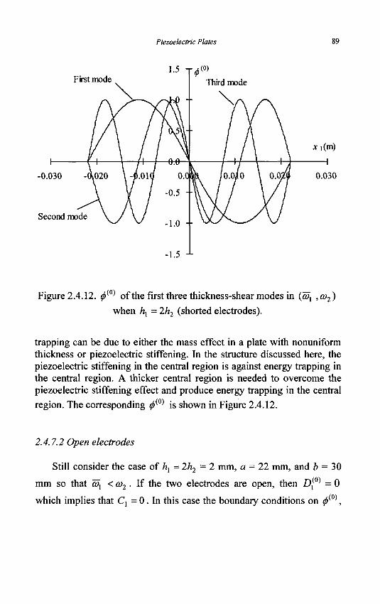
Piezoelectric Plates 89
First mode
-0.030
Second mode
1.5 Td<® Third mode
0.030
Figure 2.4.12. ^ ' ofthe first three thickness-shear modes in (&>, ,co2)
when hx = 2h2 (shorted electrodes).
trapping can be due to either the mass effect in a plate with nonuniform thickness or piezoelectric stiffening. In the structure discussed here, the piezoelectric stiffening in the central region is against energy trapping in the central region. A thicker central region is needed to overcome the piezoelectric stiffening effect and produce energy trapping in the central
region. The corresponding ^(0) is shown in Figure 2.4.12.
2.4.7.2 Open electrodes
Still consider the case of hx = 2h2 = 2 mm, a = 22 mm, and 6 = 30
mm so that ~cox <a>2 . If the two electrodes are open, then Z),(0) = 0
which implies that C, = 0. In this case the boundary conditions on ^ (0),
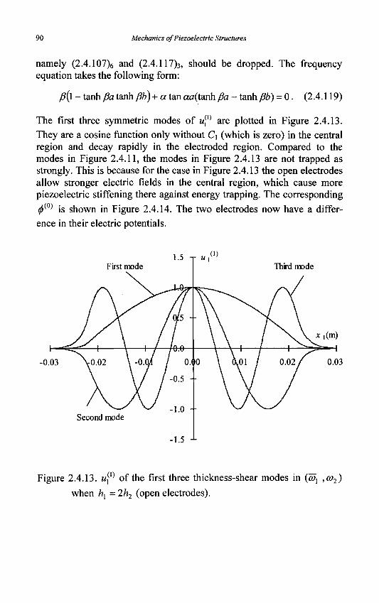
90 Mechanics of Piezoelectric Structures
namely (2.4.107)6 and (2.4.117)3, should be dropped. The frequency equation takes the following form:
fi{l - tanh Pa tanh fib) + a tan cra(tanh /3a - tanh fib) = 0. (2.4.119)
The first three symmetric modes of w,0' are plotted in Figure 2.4.13. They are a cosine function only without C\ (which is zero) in the central region and decay rapidly in the electroded region. Compared to the modes in Figure 2.4.11, the modes in Figure 2.4.13 are not trapped as strongly. This is because for the case in Figure 2.4.13 the open electrodes allow stronger electric fields in the central region, which cause more piezoelectric stiffening there against energy trapping. The corresponding
^(0) is shown in Figure 2.4.14. The two electrodes now have a difference in their electric potentials.
First mode
-0.03
Second mode
Third mode
Figure 2.4.13. w,(l) of the first three thickness-shear modes in (a>x ,a>2)
when hx = 2h2 (open electrodes).
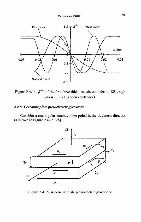
Piezoelectric Plates 91
First mode 1.5 T <j> TWrdmode
Second mode
*i(m)
0.03
-1.5 -L
Figure 2.4.14. ^(0) of the first three thickness-shear modes in (o, ,co2)
when /z, = 2/z2 (open electrodes).
2.4.8 A ceramic plate piezoelectric gyroscope
Consider a rectangular ceramic plate poled in the thickness direction as shown in Figure 2.4.15 [28].
Figure 2.4.15. A ceramic plate piezoelectric gyroscope.
92 Mechanics of Piezoelectric Structures
The plate can vibrate at the fundamental thickness-shear modes in both the x\ and the x2 directions. For a ceramic plate poled in the thickness direction ;c3, these thickness-shear modes can be excited or detected electrically by lateral electrodes on the sides at jq = ±a or x2 = ±b. Suppose a thickness-shear vibration u\ in the JCI direction is excited by a time-harmonic voltage 2Viexp(icot) applied across a pair of electrodes at x\ = ±a. If the plate is rotating about its normal with an angular rate Q, the Coriolis force F2 will excite a thickness-shear motion u2 in the x2
direction. This secondary thickness-shear will produce a voltage 2V2exp(icot) across a pair of electrodes at x2 = ±b. V2 can be shown to be proportional Q. and therefore can be used to detect O.
We are going to use an approximate procedure to analyze the gyroscope, which can be considered as a perturbation procedure [28]. For the thickness-shear motion excited by V\, the main motion is «i(1). We approximately have the following one-dimensional problem from Equation (2.4.76):
c > $ " 3C-VC4 4M, ( 1 ) - 3c-2KBl5</>f) = pu\x), I *, |< a,
^ 1 5 M U - £ ufiu = °» I X\ \< a>
r/30) = 2C{K2C^U\X) + KBu(pf ) - 0, xx = ±a,
(j>{0) = ±VX sin at, xx = ±a.
(2.4.120)
As an approximation, we neglect the piezoelectric coupling term to uxm
in the electrostatic equation in Equation (2.4.120)2. This gives an approximate solution of the driving electric potential as
^(o) ^ ^ s i n ^ ^ - ^ s i n - ^ s i n f i r f . (2.4.121) a n 2a
In Equation (2.4.121) we have approximated a linear function of x\ over [-a,a] by a sine function. It can be considered as a one-term approximation by Fourier series. This is sufficient for a qualitative study. Substituting Equation (2.4.121) into Equation (2.4.120)i, we then obtain the following expression for ux
m:
/,(1) = Bx cos—^-sincot, (2.4.122) 2a
Piezoelectric Plates 93
where
B}= 2 V J . 2
e ^ ' 2a , c o l = ^ . (2.4.123)
c44a
With M!(1) known, we have the displacement field
Wj = JC3M,(1) = Blx3 cos—-sin ^ ? (2.4.124) 2a
which leads to a Coriolis force field
/ = -2Q?3 x «,?, = ^ Q M , ^ (2.4.125)
or
f2 - -ICicoB^ cos—Lcosftrf 2a
4 TEC
s £2*05,JC3 cos erf s -2Q<aZ?,Jc3 cos—-cos&rf, n lb
(2.4.126)
where we have approximated a cosine function over [-a, a] by a constant, and similarly a constant over [-b, b] by a cosine function. With -F2 we calculate the plate resultant
n\ F 1c TCX-, Fi: = x3/jf2dx3^ p2QcoB{ cos-^-coscot. (2.4.127)
J-c 3 26 Then the boundary value problem for the thickness-shear in the x2
direction can be written as
^11^2 22 - ^ ^ ^44^2
-3c-2Kex$</>f+^jF^=pu^, \x2\<b, 2c
^is"^] - *ii#a = °> I *2 l< *» (2.4.128)
r2(30) = 2c(^2C44Mf + KBl5(/)f ) = 0, JC2 = ±b
<j>m = ±V2smwt, x2=±b,
Df = 2C(KBISU? - sn<l>f) = 0, x2 = ±b.
94 Mechanics of Piezoelectric Structures
In Equation (2.4.128) where V2 is unknown, we need some circuit condition joining the electrodes at x2 = ±b to determine V2. We consider the simple case of open circuit in which D^ or the charge, and hence the current on the electrodes, vanishes. As an approximation, we neglect the piezoelectric coupling term to 0(o) in Equation (2.4.128)]. Then, under the Coriolis force F-r*, we obtain
,0) TJX-,
B1 cos—- cos cot, 2 2b
where
B2=-2QOJ
co2-col{\ + ^ ) c^b
•Bx.
With u2m known, from Equation (2.4.128)2, we obtain
where
i (0} * • 70-7 71 . Xj <bK ' = A, sin—-coscot s — A - , —^coscot, v 2 2b 8 2 b
A.=-^B, Sexx
(2.4.129)
(2.4.130)
(2.4.131)
(2.4.132)
The mechanical boundary conditions and the open circuit condition in Equation (2.3.128) are satisfied. The electric boundary condition (2.4.128)4 gives the output voltage
v2=r\x2^b)
TZ be 15
8V3f
2Q.CO
cuc co •®«,(i + — T T )
2V3
c«b<
eX5Vx/a
c44a pc
(2.4.133)
cos cot,
Piezoelectric Plates 95
or, for voltage sensitivity
r,n 2k2-
a CD
c44b
a>„
co2-a>l(\ + ^ ) c44a
cos cot.
(2.4.134)
In Equation (2.4.133), the three pairs of brackets on the right hand side represent, from right to left, respectively, the driving of the thickness-shear motion in the x\ direction by the applied voltage V\, the driving of the thickness-shear motion in the X2 direction by the Coriolis force, and the sensing of the thickness-shear motion in the X2 direction. The roles of various material constants and geometric parameters are clearly exhibited. At resonant frequencies, the above expressions become singular. From Equation (2.4.134) it can be seen that for large voltage sensitivity, the driving frequency and the two resonant frequencies of the thickness shear motions in two directions must all be very close (double resonance). This implies that a must be very close to b and the plate is almost square. When that is the case, we can write
a>l(l + -T) = (6) + Aa)1)2,
c44a
c,,c a>l(l + -±-T) = (a> + Aco2)2,
cAib
which implies that
VXQ.
'44
-k2 b CO
2a (A<y,)(Aft)2)
(2.4.135)
(2.4.136)
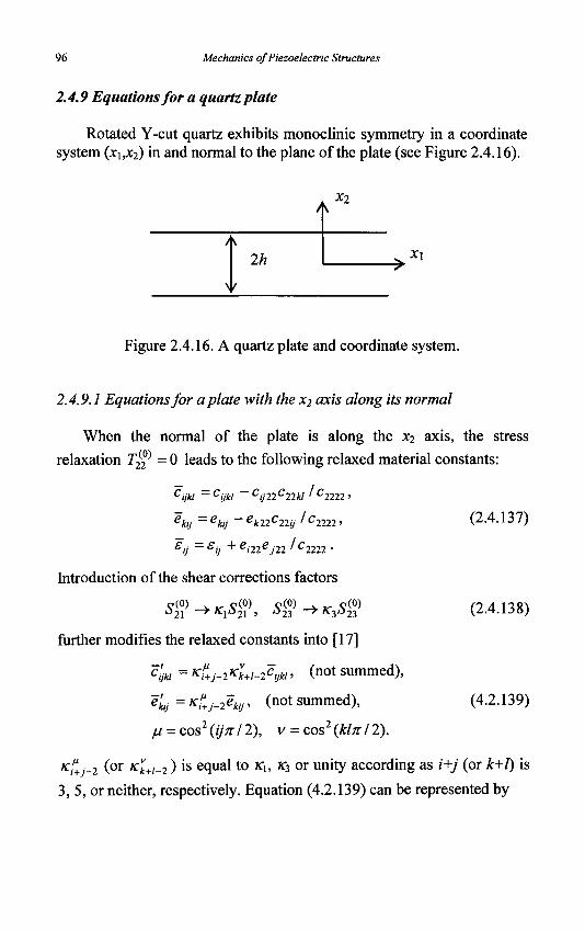
96 Mechanics of Piezoelectric Structures
2.4.9 Equations for a quartz plate
Rotated Y-cut quartz exhibits monoclinic symmetry in a coordinate system (xlrK2) in and normal to the plane of the plate (see Figure 2.4.16).
A * 2
2h • > X l
v
Figure 2.4.16. A quartz plate and coordinate system.
2.4.9.1 Equations for a plate with the X2 axis along its normal
When the normal of the plate is along the x2 axis, the stress
relaxation T^ = 0 leads to the following relaxed material constants:
Cijkl -Cijkl ~Cij22C22kl ' C2222 '
Ckij = ekij - ek22^22ij / c2222> (2.4.137)
£'j ~S'J + e'22ej22 ' C2222 •
Introduction of the shear corrections factors
S £ > - > r f , Sg>->*,Sg> (2.4.138)
further modifies the relaxed constants into [17]
c'm = K?+J_2Kvk+l_2cm' ( n o t summed),
e'ky =K?+J_2eklJ, (not summed), (4.2.139)
ju = cos2 (ijn 12), v = cos2 {kin 12).
Kilj-2 (o r Kk+i-2) is e ( l u a l t 0 Ki> K* or unity according as /'+/' (or k+I) is
3, 5, or neither, respectively. Equation (4.2.139) can be represented by
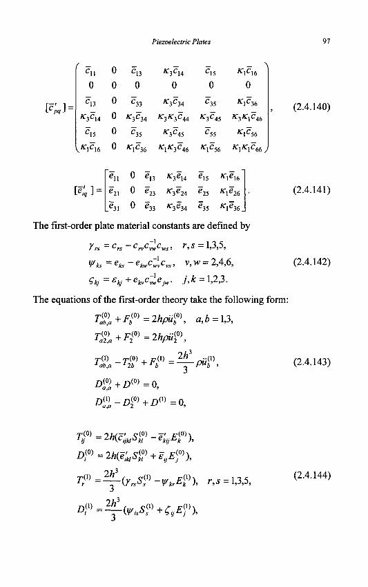
Piezoelectric Plates 97
PL1 =
Cll
0
Cis
"r3C14
^,5
v,K lC16
0
0
0
0
0
0
C13
0
C33
K'3C34
^35
K\C16
K-,C 3M4
/C,C 3"-34
/C,C 3M5
-15
'35
'55
K,C _ \ 16
K,C 1^36
R r3K '3C44 K :3C45 X r3K r iC46
lc36 K\K3CA6 K\C56 K\K\C66
(2.4.140)
\e'iqV K-,e 3C14
=21
'31 0 '23
=33
/r,e 3C24
K,e-3*=34
=15
=25
=35
K,e lc16
K\e lc26
/c,e lc36
The first-order plate material constants are defined by
-co c ** rr" mr'ws *
(2.4.141)
Yrs Crs C rvC vt»C v/s •> r>S ^ P ?
Vks = eb - C*M.C^C» > v ' w = 2'4>6, (2.4.142)
S# = £kj + eivCvweyw • 7> * = 1)2,3.
The equations of the first-order theory take the following form:
TJ&+F™=lhpuf>, a,b = \,3,
TZ+F^=2hpiif\
1ab,a~12b + r b ~
2h3
•m a)
z > £ > + / ) ( « > = a, id) l(0) D%-D?>+D™=0, id ) - 1
(2.4.143)
T(0) =2h(c' S(0) -e' Ei0)) 1ii An\ciikl°kl ekiirjk h
l (0)
'ijkl^kl
A w =2*g^+* ,£™) ,
kij^k
&=— {YrSS?-VkrE?), r,s = 1,3,5, 3
3 Aw=^-(^«+^«X
(2.4.144)
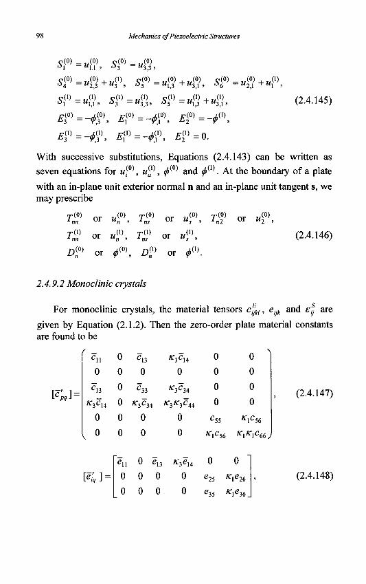
98 Mechanics of Piezoelectric Structures
S<°>
s™
sf EP
£3(1)
_ u (0) o(0) _ (0) — Mj ] , O3 — «3 3 ,
- « 2 , 3 + M 3 ' ° 5 _ " 1 , 3 + M3,1> ° 6
_ ,.(i) oO) _ „(l) c(l) _ „ 0 ) . „(l) _ " U ' ° 3 _ M 3,3> ° 5 - M 1 , 3 + M 3 , 1 '
= -^30), ^ ( 0 ) =^f . ^ f ^ - ^ , = -<Pf, Ell)=-*$\ E?=0.
= «£?+«i0)
(2.4.145)
With successive substitutions, Equations (2.4.143) can be written as
seven equations for , ^ ( 0 ) and ^ ( 1 ) . At the boundary of a plate
with an in-plane unit exterior normal n and an in-plane unit tangent s, we may prescribe
r ( 0 ) nn
nn
or u (0)
or u (i)
or ^ (0)
r ( 0 ) 1 ns
T® or u
or wo
(i)
(0) r ( 0 ) or w
(0)
or (/)
s ' (1)
(2.4.146)
2.4.9.2 Monoclinic crystals
For monoclinic crystals, the material tensors cfjkl, eijk and stj are
given by Equation (2.1.2). Then the zero-order plate material constants are found to be
P;J=
Cn
0
^13
K"3C14
0
, o
[*;]=
0
0
0 0
0
0
«ii 0
0
Cl3
0
C33
ff3C34
0
0
0
0
0
g13
0
0
K"3C14
0
^3C34
0
0
K"3e]4
0
0
0
0
0
0
C55
( )
0
0
0
K\C56
/ f ,C5 6 /C^jCgg^,
0 g25
*35
0
" : l e26
^1^36 .
?
(2.4.147)
(2.4.148)
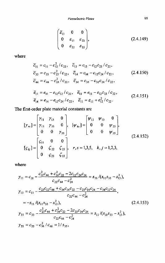
Piezoelectric Plates 99
0 0
where
0
0
C l l _ C l l C12 ' C 2 2 >
;32
'23
'33
'13 " C 12 C 23 ' C 2 2 '
-33 — C33 CyilCyy, C,A—CU C\lC2b ' C 22 »
c44 = c. 44 C24 ' C22 ' C34 — C34 C32C24 ' C22 '
e\l — eU g 1 2 C 1 2 ' C 2 2 ' g13 — g13 e 1 2 C 2 3 ' C 2 2 »
2 ?14 - g14 e 12 C 24 ' C 2 2 » Ml : £ 1 1 + e 1 2 ' C 2 2 -
The first-order plate material constants are
where
Yu ~ cn -
?M3 = C13 ~~
Y\\ Yn 0
Yn Y33 0
0 0 y55
gu 0 0
0 S 22 ^23
" ?23 ^33
[^*J: Vll ^13 0
0 0 l//25
0 0 ¥l5
r,s = 1,3,5, Ar,7 = 1,2,3,
C 12 C 44 + C 1 4 C 2 2 ^C12CUCH
C-,-,C - S33 ' v M l 5 3 3 5 1 3 ) '
22^44 '24
C 23 C 12 C 44 + C 3 4 C 1 4 C 2 2 C 23 C 14 C 24 C 34 C 12 C 24
^22^44 ^ 24
5 ] 3 / ( 5 n 5 3 3 S 1 3 ) ,
^33
^55
^ 3 3 -
2 2 C23C44 + C34C22 ' -^C23C3AC24
C22C44 C
• su /(sns33 su)>
24
: C55 C56 ' C 66 — 1 ' 5 5 5 '
(2.4.149)
(2.4.150)
(2.4.151)
(2.4.152)
(2.4.153)
100 Mechanics of Piezoelectric Structures
_ e12VC12C44 C 1 4 C 2 4 ) + g14 (C14C22 C12C2A) H I ~eU ^~2
C22C44 ~ C 2 4
= duyu+duyu,
... _„ e12(C32C44 ~ C 3 4 C 2 4 ) + e14VC34C22 ~ C 3 2 C 2 4 ) ,« . u ,N
r i 3 _ e 1 3 2 ( / . 4 . 1 3 4 )
C22C44 ~ C 2 4
= d\\Y\l + ^13^33»
^ 2 5 ~ g 2 5 — g26C56 ' C 6 6 '
^ 3 5 = g 3 6 - e 3 6 C 5 6 ' C66 = " 3 5 / 5 5 '
_ ^12C44 + e14C22 2e1 2e1 4C24 S»II _ * l l +
C22C44 C24
2 C22 =£22 +g26 /c66> (2.4.155)
«3 = £V> + e26g36 ' C66 >
^ 3 3 = £ 3 3 + e 3 6 / c 6 6 .
The constitutive relations are
Tr = 2h(cuS^ +c135<°> +* ,c I 4 Sf - e „ J f >),
rW =2/Kc1351(0) +c 3 3 ^ 0 ) + ^ c 3 4 5 f - e 1 3 ^ 0 ) ) ,
r4(0) = 2/Z(K3C14S,(0) + K3C34S3
(0) + *r32c44S<0) -K3e14El0)), (2.4.156)
7 f > = 2 / ^ ^ + K 1 C 5 6 ^ > -e25E^ -e35E^),
T^ =2h(Klc56S^ +^c6X0) ~^e26E^ -Kle36EP),
A(0) =2//(eu51(0) + e13S3
(0) +K3euS\0) +enE^),
D^ = 2h{e25Sf) + Kxe2()SfUe22E^ +s23E^\ (2.4.157)
A(0) = 2h(e35Sr) + r , ^ + **#«> + ^ X
(2.4.159)
Piezoelectric Plates 101
7 f =^-(VuSll) +7^l) -¥nE\x)\ (2.4.158)
D^=^(WnS^+¥uSfU^nEn
The equations of motion and charge take the following form:
C11M1,11 + C55M1,33 + (*"lC56 + /£ -3C14)M2,13 + (C13 "•" C55 )M3,31
+ cii^ff + e35j<g + K3CU4} + KXC56U$ (2.4.160)
2«
( f flC56 +" r3C14)M l ,13 +K\ C66M2,11 + ^ 3 C44W2,33
+ ^Cs6«3?n +^3C34"3033 + (*1«36 + K3 «14 M i ? (2.4.161)
+ r 2 c M ( 1 ) + K - 2 C w ( 1 ) + * - e M( 1 )+JLj r ( ° ) - ™ ( 0 )
2«
(C5 5 + C 1 3 ) M 1 1 3 + ^ i C 5 6 M 2 j l l + *3C34M2,33 + C55M3,11 + C33M3,33
+ (e35 + e13 #g> + J C ^ I I } ? + i ^ i / g (2.4.162)
+ e 2 5 t f ) + ^ 3 ( 0 ) = ^ ° ) , 2«
102 Mechanics of Piezoelectric Structures
e l l M l , l l + e 1 5 M l , 3 3 +\K\e16 + K3e\4 )M2,13 + (^13 + e 3 5 )M3,31
+ Kxe,6uf} + K3euu™ - enj$ + e ^ (2.4.163)
_ f f ^ ' ) + _ L Z ) ( 0 ) = o ) 23 V,3 2 ^
rn"ui +yS5«u3 +(/i3 +r55)"3!3i +^n^.iV +^35^3 - 3 /T 2
[KXC56 («<»> + «<°>) + K2XC66 («<»> + M,(1)) (2 .4 .164)
^_
2tf + Kie2J
m +Klei6<f>f] + -^JFl
m=pull\
(Tn + r5s )«1 .31 + Visual + 73iU3% + ( ^ 1 1 + ^35 ¥,13
-3h-2[K3cuu™ +K3C„U™ +K23C4M°I
+M31)) (2.4.165)
In
VllWui +^35«1(,33 + (^13 + ^ 3 s K 3 1 " f l l ^ Y " ?33^.33
- S A " 2 ^ ^ + <1))W26(t40
1) +Wl
(,)) (2.4.166)
- ^ ' ) - ^ 0 ) ] + - ^ ^ ( 1 ) = o . 2«
2.4.10 A quartz piezoelectric resonator
We now revisit the thickness-shear vibration problem of a quartz plate analyzed in the first section of this chapter using the three-dimensional equations. Consider a rotated Y-cut quartz plate as shown in Figure 2.4.17.
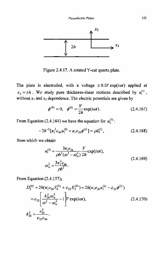
Piezoelectric Plates 103
2h
X2
X\
Figure 2.4.17. A rotated Y-cut quartz plate.
The plate is electroded, with a voltage ± 0.5V exp(i cot) applied at
x2 =±h . We study pure thickness-shear motions described by w,05 ,
without JCi and JC3 dependence. The electric potentials are given by
^ ( 0 ) = 0 , (/>m =— exp(icot). 2h
From Equation (2.4.164) we have the equation for w,(1):
-3h-2[K?c66uii)+Kle2jW] = pu?\
from which we obtain
« f ' > = - 3 y i g 2 6
ph\<ol-a>^2h exp(icot),
co„=-3K, C. 66
ph2
From Equation (2.4.157)2
£><°> =2h(Kle26S?) +s22E?)) = 2h(<Kxe26uV -s22^)
V expQcot), = £ 22 *2
26<y» _ j
*26
2 2
= 26
E-nC,
(2.4.167)
(2.4.168)
(2.4.169)
(2.4.170)
22^66
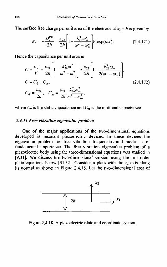
104 Mechanics of Piezoelectric Structures
The surface free charge per unit area of the electrode at x2 = h is given by
<r„ = -Z>«°> "22
2h 2h co2-col V exp(icot). (2.4.171)
Hence the capacitance per unit area is
22 c = - = £
V 2h
2 , . 2 k^co, 26 "'oo
co2-col
c = c0+cm,
C 0 = ^ 0 2h
„ g22
~ 2h
_ f22 "-26 ^ K m i i 2 2
2h co —L co„
4^ 2(co -cox)
(2.4.172)
where Co is the static capacitance and Cm is the motional capacitance.
2.4.11 Free vibration eigenvalue problem
One of the major applications of the two-dimensional equations developed is resonant piezoelectric devices. In these devices the eigenvalue problem for free vibration frequencies and modes is of fundamental importance. The free vibration eigenvalue problem of a piezoelectric body using the three-dimensional equations was studied in [9,31]- We discuss the two-dimensional version using the first-order plate equations below [31,32]. Consider a plate with the x2 axis along its normal as shown in Figure 2.4.18. Let the two-dimensional area of
X2
2h xi
Figure 2.4.18. A piezoelectric plate and coordinate system.
Piezoelectric Plates 105
the plate be A and the boundary curve of A be C, and C be partitioned as
CUUCT=C4<JCD=C,
CunCT=C^nCD=0. (2.4.173)
The eigenvalue problem for free vibrations of a piezoelectric plate by the first-order theory is
-rj°j=fl>22A/w<0) in A,
-T^b+T^=co2^-pu^ in A, ba,b la 3 H a (2.4.174)
-Dff=0 in A, -D%-DF>=0 in A,
-Sl°>+\(«%+»?2+*„«?+*„«?>) = (> in A,
-^ )+}(«S+«S) = ° in 4 (2.4.175) £ ( ° ) + ^ ° ) + ^ ( 1 ) = 0 in A,
E®+$=0 in 4
-T}»+2h(jr9US<»-e^E^O in J,
9fo3 (2.4.176) -^(,)+^-(r^«-^£C.)) = 0 in A,
D}0)-2Ke^S^+evE^) = 0 in 4
9/J (2.4.177)
106 Mechanics of Piezoelectric Structures
- " , ( 0 ) =0 , - « «
njT}P=0, nbT^=Q on CT,
- , < • > - * - , » = . o„ c (2A178)
n,D<»=0, naD^=0 on CD.
We look for values of a>2 corresponding to which nontrivial solutions exist. For convenience we introduce the following vector U:
cm cO) E-(O) Fmx
and operators A and B:
ATT _ L T ( » ) _T<U +r(°> - n<°> - n® - n^
- ^ 4 ( « 8 +«ffi). ^0)+*S0) + ^ 0 ) , ^ +#S (1)
2
(2.4.179)
7 ^ 4 - 2 ^ , ^ - ^ 0 , (2.4.180)
2h3
BU = {2hpuf\—puf,0,0,0,0,0,0,0,0,0,0}. (2.4.181)
We also define
YiA) = {U | Equation (2.4.178) is satisfied}. (2.4.182)
With the above definitions, the eigenvalue problem can be stated as: Find X = o)2 for which there exists a nontrivial U € ~L(A) such that
AU = ABU. (2.4.183)
Piezoelectric Plates 107
For two vectors U,Ve S(^4), we introduce an inner product
<U;V>= f ( w ^ + w ^ W V W V 0
+ T^Gf +T^G^+D^B^ +D®B® (2.4.184)
where U is given by Equation (2.4.180) and
p(o) c-0) r ( 0 ) r ( i )> J ij >* ba ' * - ; J * - a i •
(2.4.185)
For two vectors U,Ve E(^4), it can be shown by integration by parts that
<AU;V>=<U;AV>, (2.4.186)
<BU;V>=<U;BV>.
Therefore the operators A and B are self-adjoint. This is consistent with the self-adjointness of the three-dimensional operators [9] from which the plate equations are derived. With the above formulation in terms of the abstract vectors and operators, it can be shown in the manner of [9] that the eigenvalues are real and the eigenvectors associated with distinct
eigenvalues A(m) and ^(n) are orthogonal:
< AU(m); U(n) >= 0, < BU(m); U(n) >= 0, m*n. (2.4.187)
With the abstract formulation, in a way similar to [9], it can also be shown that the Rayleigh quotient of the variational formulation of the eigenvalue problem is
n ( U ) = < A U ; U > . (2.4.188) <BU:U> '
2.5 Second-Order Theory
In this section we explore the effects of the second-order terms in the power series expansion. A second-order theory is outlined, and several special cases of the second-order theory are examined.
108 Mechanics of Piezoelectric Structures
2.5.1 Equations for second-order theory
A second-order theory describes coupled extensional (w^0), a = 1,2),
flexural ( u^0) ), fundamental thickness-shear (i/p ), thickness-stretch
(w^) , and symmetric thickness-shear (w„2)) motions of a plate. For the
electrical behavior of the plate, we consider ^ ( 0 ) , 0m and ^ ( 2 ) . The
approximate displacement and potential fields are
(2.5.1)
We have included a few additional displacement components in Equation (2.5.1). «32) and u*p represent the thickness stretch or contraction due to Poisson's effect. From Equations (2.2.6) and (2.2.7) it can be seen that M^2) together with w^3) contribute to thickness-shear deformations S^ and IS,J2) which may couple to the other second-order strains due to anisotropy. The two-dimensional plate equations we will obtain are for u\0), u*p and u^ only. Other displacements will be eliminated through stress relaxations. Within the approximation in Equation (2.5.1), the strains and electric fields in Equations (2.2.5) through (2.2.10) become:
<?(0) _ ,.(0) o(0) _ (0) r.(0) _ (1) °1 — "1,1 ' °2 — "2,2 > ° 3 — "3 '
55°>=iA)+^>, 5<o)=^)+«p>, ^°)=«a)+«4?, (2.5.2)
Oi — Mi i , *J2 — ^ 2 2 ' 3 — 3 5 (2.5.3)
1 — ^ 1 1 > 2 — ^ 2 2 ' 3 — ^ ^ 3 ?
S<2)=ug+3i43), S<2>=i4J+3«f3), S<a>=ug) + iS ) , (2'5'4)
E<0) = -$\ 40)=-$\ Ef^-f\ (2.5.5)
Piezoelectric Plates 109
E^=-^\ E? = -$, E^ = -2^2\ (2.5.6)
E™=-$\ E? = - $ \ £3(2)=0. (2.5.7)
Higher order strains S^p are neglected. From Equation (2.2.17)i we
obtain
« ^ l ° ) = 2 ^ r + y r f )! o,6 = 1A
TZ+F^ = 2hpii?\
TZ-T^ + FP^puV, (2.5.8)
where we have truncated the right hand sides by keeping the inertial terms of the displacement components of interest only. Equation (2.5.8)i is for extension, Equation (2.5.8)2 is for flexure, Equation (2.5.8)3 is for the fundamental thickness-shear, Equation (2.5.8)4 is for the fundamental thickness-stretch, and Equation (2.5.8)5 is for the symmetric thickness-shear. For the charge equations of electrostatics we have, from Equation (2.2.17)2, for an unelectroded plate:
D^-D^+Dm=0, (2.5.9)
Zj£>-2Z#>+i)<2>=0.
The case of an electroded plate will not be examined. In fact, in higher-order theories, when electrodes are present, it is more convenient to use two-dimensional charge equations obtained by the polynomial expansion of $ in Equation (2.2.18).
110 Mechanics of Piezoelectric Structures
For plate constitutive relations we truncate Equation (2.2.12) as
(2.5.10) 7 f = 2h{cljklS^ - eklJE^) + ^(cijklS™ - ekiJE™),
A(0) = 2h(eukS$> + svEf) + f( > + s,E?),
*y - \cijkl^kl ekijEk )>
^/ -^r~(cyki^ki ~ekijEk ) + ~j~(cijkiSki ~ekijEk ) '
^2) = ( r f ^vEf^) + f(eukSf + svEf),
(2.5.11)
(2.5.12)
where SJp has been neglected. Since Syl) contains i^2) and £^2)
contains Wj2) and w((3), Equations (2.5.10) through (2.5.12) are not yet
ready to be used. To obtain the proper constitutive relations we need to make the following stress relaxations:
L (2-5.13) 7?
(2)=0, ? = 3,4,5,
from which expression of S3(1), S3
(2), S\2) and SJ2) in terms of other
strain components can be obtained to eliminate Wj2) and uf in
Equations (2.5.10) through (2.5.12). Then Equations (2.5.8) and (2.5.9)
can be written as eleven equations for w,-0), u(P , w„2), ^ ( 0 ) , ^(1) and
^(2) . In order to predict the exact cutoff frequencies for the two
fundamental thickness-shear, the fundamental thickness-stretch, and the two symmetric thickness-shear modes, five correction factors will be needed.
Piezoelectric Plates 111
2.5.2 Extension, thickness-stretch and symmetric thickness-shear
To examine the basic behaviors of the second-order equations, we study the special case of an isotropic elastic plate. In this case the second-order equations decouple into two groups. One is for coupled flexure and fundamental thickness-shear, and the other is for coupled extension, thickness-stretch, and symmetric thickness-shear. The former has been discussed in the fourth section of this chapter. We explore the latter below.
It is obvious that when a plate is in extension there is thickness stretch or contraction due to Poisson's effect. At the low frequency range this thickness deformation can be approximately determined from the stress relaxations in the zero-order theory, i.e., Equation (2.3.15) or Equation (2.3.23). When the frequency gets higher or close to the fundamental thickness-stretch frequency, resonance of the thickness-stretch vibration needs to be considered. In addition, high frequency extensional waves become dispersive (see Figure 2.1.4).
First-order, two-dimensional plate equations governing coupled extensional and thickness-stretch motions of plates are due to Kane and Mindlin [33]. This theory includes the resonance of the fundamental thickness-stretch mode and can predict the dispersion of high frequency extensional waves. The equations of the Kane-Mindlin theory can be reduced to the classical equations of extension for low frequencies and long waves [13]. However, the Kane-Mindlin theory has a serious flaw. It cannot predict a complex branch of the dispersion curve that the three-dimensional theory predicts to exist in the frequency range of interest [34]. It was also shown in [34] that in order to capture this complex branch the second order effect of symmetric thickness-shear has to be included. Equations for elastic plates in coupled extension, thickness-stretch and symmetric thickness-shear motions are due to Mindlin and Medick [34] using polynomial expansions. Two-dimensional equations containing extensional, thickness-stretch, and symmetric thickness-shear and higher-order modes were also obtained in [19] using trigonometric expansions. The equations for extensional, thickness-stretch, and symmetric thickness-shear in [19] are equivalent to the Mindlin-Medick theory in that their dispersion curves have the same geometric structure. In the following we will use the equations in [19] for which the correction factors have been determined.
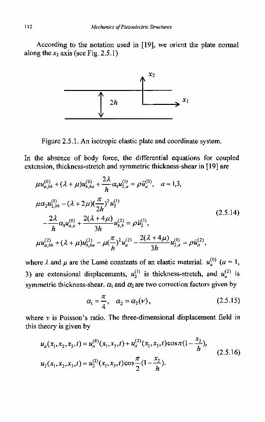
112 Mechanics of Piezoelectric Structures
According to the notation used in [19], we orient the plate normal along the x2 axis (see Fig. 2.5.1)
/\ 2h
X2
Xl
Figure 2.5.1. An isotropic elastic plate and coordinate system.
In the absence of body force, the differential equations for coupled extension, thickness-stretch and symmetric thickness-shear in [19] are
2X Mu%b + (A + Ml, + —ml>, = pu™, a = 1,3,
h
jua2u^bb-(A + 2M)(^-)2u^ in
2X ,(°) — 7 - « l « ^ + h
2(A + 4M)A2) _ (2.5.14)
3h *b,b P4\
Mua,bb +(A + M)ub,ba M T V U" Ti 2,a ~ PUa '
h 3«
where X and JU are the Lame constants of an elastic material. u(a ' (q= I,
3) are extensional displacements, U™ is thickness-stretch, and w<2) is
symmetric thickness-shear. a,\ and a2 are two correction factors given by
71 « i = 7 > <h = ch.<y)> (2.5.15)
where v is Poisson's ratio. The three-dimensional displacement field in this theory is given by
ua^,x2,x3,t) = i£0)(xi,*3,0 + K J(x„of3,Ocos^(l--f), n
.,(1)/.. „ *\~~„n ft X2-
(2.5.16)
u2(xvx2,x3,t) = u\ )(x1,x3,/)cos—(1 — - ) . 2 n
Piezoelectric Plates 113
The plate resultants are given below. Those associated with extension are
T^ = (A, + 2M)u^ + Xuf] + —4\ h
r3(30) = (A+ 2ju)4°i + Xu\y +—4l\ (2.5.17)
r1f = M4°3)+<,))-
The two self-equilibrating shear resultants T$ for thickness-stretch are
T$ = aMl+^\ (2.5.18) in
while the second-order resultants are given by
3«
T3f =(Z+2M)u™ + Xu\2) ~ u ? , (2.5.19) 3«
TS^rt-S'+«£?)• We now consider straight-crested waves propagating in the xi
direction (d /Sx3 = 0). Furthermore, we look for solutions in which M30) = «32) = 0. Then, Equations (2.5.14) reduce to
(A + 2M)uW+^arfl=pii?\ h
^a2u%-(A + 2ju)(—)2u^ 2h
2X a,u>V +—^-
3h aiUv)+m±Wu$ = piim,
(2.5.20)
Let
(A + 2M>e\ - M&u™ - ^ - ^ ' 1 = Puf\ n in
M,(0)=4(0)expi(£,-ffl0,
M}2) = 42) expi(£, - a*), (2.5.21)
4 ° = - i ^ exp/(£t, - cot),
114 Mechanics of Piezoelectric Structures
so that Equations (2.5.20) yield
h
jua2(-A?f)-(A+2M)(-?-)2A2A)
2h
+ 2AaxA^ - M ± M 4 ( ^ = .rf^ h in
(A + 2MX-Al»e)-M£f4V h
For nontrivial solutions, we have
r r - f i ' -(k-2)x -(k2-2)X k2 + a2X
2-Q.2
3TT
0
(k2 + 2)X
—(r + 2)x r r + 4 - Q ' 3^-
where we have used the notation
X = 2%h
n
A + 2ju
Q = co/(^), 2h
E p'
k2=\ = 2-v2 \-2v
(2.5.22)
- 0 , (2.5.23)
(2.5.24)
vi and V2 are the speeds of longitudinal and transverse plane waves in an unbounded, isotropic elastic body, respectively. Equation (2.5.23) determines the dispersion relations for coupled extension, thickness-stretch, and symmetric thickness-shear modes of the plate. These dispersion curves are shown in Figure 2.5.2 for v = 0.25 and a,j= 0.845.
Besides being able to describe the slope and curvature of the dispersion curve for long thickness-stretch waves at frequencies close to the first thickness-stretch frequency, Equation (2.5.23) can also predict the complex branch of the dispersion relation that was missing in the Kane-Mindlin theory. We have the following local, asymptotic
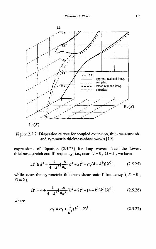
Piezoelectric Plates 115
\m{X)
Figure 2.5.2. Dispersion curves for coupled extension, thickness-stretch and symmetric thickness-shear waves [19].
expressions of Equation (2.5.23) for long waves. Near the lowest thickness-stretch cutoff frequency, i.e., near X = 0, Q = k , we have
Q2^k2 1-^[—(k2+2)2-a3(4-k2)]X2, (2.5.25) 4 -k 9n
while near the symmetric thickness-shear cutoff frequency ( X = 0 , Q = 2),
Q2 « 4 + _ L ^ _ ^ U y f c 2 + 2 ) 2 +(4-k2)k2]X2 , (2.5.26)
4-& 2 9n2
where
a 3 = a 2 + - ! r ( A : 2 - 2 ) 2 . (2.5.27)
116 Mechanics of Piezoelectric Structures
We note that Equations (2.5.25) and (2.5.26) break down when A?= 4 or v = 1/3; this represents the degenerate case when the lowest thickness-stretch frequency coincides with the symmetric thickness-shear frequency.
2.5.3 Elimination of extension
For long waves at frequencies close to the first thickness-stretch frequency Q = k , an approximation can be made to eliminate the coupling to extension [35]. Dropping the term quadratic in £, in Equation (2.5.22)! for long waves and setting Q = k , we obtain
A^=-h 2X
4>t,
which is equivalent to
,(°) h 2X
K X + 2jU
(2.5.28)
(2.5.29)
Substitution of Equation (2.5.29) into Equations (2.5.20)2;3 yields the following equations for coupled thickness-stretch and symmetric thickness-shear:
,,(') *N2..(1) . 2Q*+ 4/Q .,(2) _ «l,l ' = PU2^ fiaAl -0* + 2/iX—)z« ,J + - ^ —
2« 3«
(X + 2M)u™ - M£fU™ - ^ - ^ = Pu?\ h 3«
(2.5.30)
Now, letting
u\2) = A[2) e x p / ^ j - art),
u^ - -iA^ exp/'(£<;, - ox),
we obtain the following dispersion relation from Equation (2.5.30):
4
(2.5.31)
a3X'+k* & 3TT
(kl+2)X
—(k2+2)X k2X2+4-Q2
3n
= 0. (2.5.32)
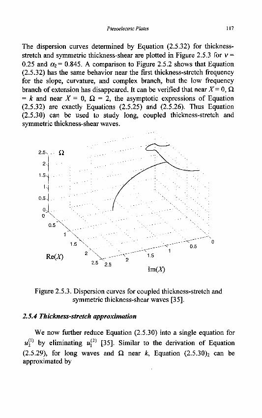
Piezoelectric Plates 117
The dispersion curves determined by Equation (2.5.32) for thickness-stretch and symmetric thickness-shear are plotted in Figure 2.5.3 for v = 0.25 and a2= 0.845. A comparison to Figure 2.5.2 shows that Equation (2.5.32) has the same behavior near the first thickness-stretch frequency for the slope, curvature, and complex branch, but the low frequency branch of extension has disappeared. It can be verified that near X= 0, Q = k and near X = 0, Q = 2, the asymptotic expressions of Equation (2.5.32) are exactly Equations (2.5.25) and (2.5.26). Thus Equation (2.5.30) can be used to study long, coupled thickness-stretch and symmetric thickness-shear waves.
2.5X a
2,.
1.5
1
0.5-
0 0 " \
0.5 ~
1.5 0.5
Re(X) 2.5 2.5
1.5
Im(J0
Figure 2.5.3. Dispersion curves for coupled thickness-stretch and symmetric thickness-shear waves [35].
2.5.4 Thickness-stretch approximation
We now further reduce Equation (2.5.30) into a single equation for
u^p by eliminating w[2) [35]. Similar to the derivation of Equation
(2.5.29), for long waves and Q. near k, Equation (2.5.30)2 can be approximated by
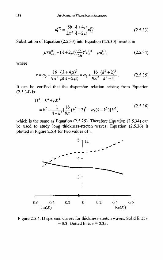
118 Mechanics of Piezoelectric Structures
(2) _ Sb X + A^i 1 ~ 3 ; r 2 / l - 2 / /
(2.5.33)
Substitution of Equation (2.5.33) into Equation (2.5.30)i results in
In
where
r = a, + 16 (A + 4{i)
-a3 + 16 (k2+2)2
3 ' 9K2 M(*-2M) ~l ' 9x2 k2-4
(2.5.34)
(2.5.35)
It can be verified that the dispersion relation arising from Equation (2.5.34) is
Q2=k2+rX2
= k2-2 l l¥-(k2
+2f-a3(4-k2)]X2, (2.5.36)
4-k2 9n
which is the same as Equation (2.5.25). Therefore Equation (2.5.34) can be used to study long thickness-stretch waves. Equation (2.5.36) is plotted in Figure 2.5.4 for two values of v.
5 -|
4 -
3 -
i 1 i I i i i
-0.6 -0.4 -0.2 0 0.2 0.4 0.6 Im(X) Re(X)
Figure 2.5.4. Dispersion curves for thickness-stretch waves. Solid line: v = 0.3. Dotted line: v = 0.35.
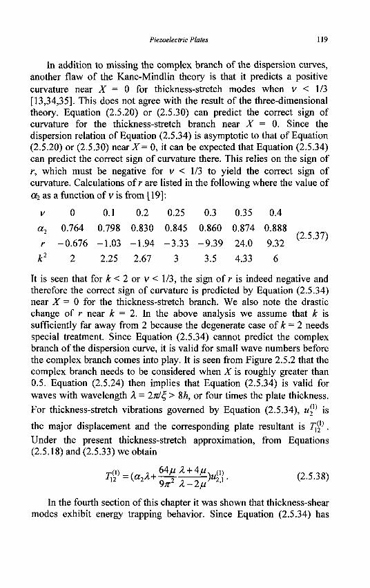
Piezoelectric Plates 119
In addition to missing the complex branch of the dispersion curves, another flaw of the Kane-Mindlin theory is that it predicts a positive curvature near X = 0 for thickness-stretch modes when v < 1/3 [13,34,35]. This does not agree with the result of the three-dimensional theory. Equation (2.5.20) or (2.5.30) can predict the correct sign of curvature for the thickness-stretch branch near X = 0. Since the dispersion relation of Equation (2.5.34) is asymptotic to that of Equation (2.5.20) or (2.5.30) near X= 0, it can be expected that Equation (2.5.34) can predict the correct sign of curvature there. This relies on the sign of r, which must be negative for v < 1/3 to yield the correct sign of curvature. Calculations of r are listed in the following where the value of Cfe as a function of v is from [19]:
v 0 0.1 0.2 0.25 0.3 0.35 0.4
a2 0.764 0.798 0.830 0.845 0.860 0.874 0.888 2 (2.5.37) r -0.676 -1.03 -1.94 -3.33 -9.39 24.0 9.32
k2 2 2.25 2.67 3 3.5 4.33 6
It is seen that for k < 2 or v < 1/3, the sign of r is indeed negative and therefore the correct sign of curvature is predicted by Equation (2.5.34) near X = 0 for the thickness-stretch branch. We also note the drastic change of r near k = 2. In the above analysis we assume that k is sufficiently far away from 2 because the degenerate case of k = 2 needs special treatment. Since Equation (2.5.34) cannot predict the complex branch of the dispersion curve, it is valid for small wave numbers before the complex branch comes into play. It is seen from Figure 2.5.2 that the complex branch needs to be considered when X is roughly greater than 0.5. Equation (2.5.24) then implies that Equation (2.5.34) is valid for waves with wavelength A = 2n/% > $h, or four times the plate thickness. For thickness-stretch vibrations governed by Equation (2.5.34), u^ is
the major displacement and the corresponding plate resultant is T$.
Under the present thickness-stretch approximation, from Equations (2.5.18) and (2.5.33) we obtain
Ty=(a2^^)u%. (2.5.38)
In the fourth section of this chapter it was shown that thickness-shear modes exhibit energy trapping behavior. Since Equation (2.5.34) has
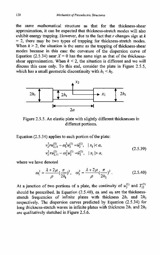
120 Mechanics of Piezoelectric Structures
the same mathematical structure as that for the thickness-shear approximation, it can be expected that thickness-stretch modes will also exhibit energy trapping. However, due to the fact that r changes sign at k = 2, there may be two types of trapping for thickness-stretch modes. When k > 2, the situation is the same as the trapping of thickness-shear modes because in this case the curvature of the dispersion curve of Equation (2.5.34) nearX= 0 has the same sign as that of the thickness-shear approximation. When k < 2, the situation is different and we will discuss this case only. To this end, consider the plate in Figure 2.5.5, which has a small geometric discontinuity with hi < h2.
2h2
i
i
t
i 2hi
k
hi T i
i
2/7
r
k-2a
-H
Figure 2.5.5. An elastic plate with slightly different thicknesses in different portions.
Equation (2.5.34) applies to each portion of the plate:
v?rc4')i - <«i2z41) =i$\ I *i |< a, •*2,11
„0) 1 2
,2„0) v2ru\;u-co2u\
*2 >
um
where we have denoted
2 X+2n, n 2
p 2\ "i CD-, X + 2y n 2
p 2h~,
(2.5.39)
(2.5.40)
At a junction of two portions of a plate, the continuity of u2l) and T$
should be prescribed. In Equation (2.5.40), a>\ and Gh are the thickness-stretch frequencies of infinite plates with thickness 2hx and 2h2
respectively. The dispersion curves predicted by Equation (2.5.34) for long thickness-stretch waves in infinite plates with thickness 2h\ and 2h2
are qualitatively sketched in Figure 2.5.6.
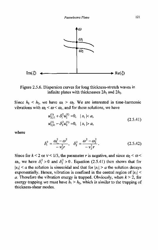
Piezoelectric Plates 121
Im($ <- - • R e ( £
Figure 2.5.6. Dispersion curves for long thickness-stretch waves in infinite plates with thicknesses 2h\ and 2h2.
Since h\ < h2, we have (0\ > (Oi- We are interested in time-harmonic vibrations with ah < <o< Oh, and for these solutions, we have
where
tt^n + sfu^ =°> I *i l< a>
u^-S^^O, \xx\>a,
2 2 2 2 o2 CO, -G) 2 0) -0)2
°\ = 1 " ' S2 = 2—
-v-,r -v-,r
(2.5.41)
(2.5.42)
Since for k < 2 or v < 1/3, the parameter r is negative, and since a>1< (0< a>\, we have £,2 >0 and 8\ > 0 . Equation (2.5.41) then shows that for 1*11 < a the solution is sinusoidal and that for |*i| > a the solution decays exponentially. Hence, vibration is confined in the central region of |*i| < a. Therefore the vibration energy is trapped. Obviously, when k > 2, for energy trapping we must have hi > h2, which is similar to the trapping of thickness-shear modes.
Chapter 3
Laminated Plates and Plates on Substrates
Piezoelectric plates are often attached to or embedded in elastic plates for various applications. These structures can be treated in general as laminated plates. In this chapter we first analyze two special structures, i.e., an elastic plate with piezoelectric layers on one or both of its major surfaces. Then a general discussion on laminated piezoelectric plates is presented, followed by the analyses of two problems of a plate on a half-space.
3.1 Elastic Plates with Symmetric Piezoelectric Actuators
In this section, we consider the simplest case of an elastic plate with piezoelectric layers (actuators) symmetrically attached to its major surfaces. In this case, bending of the elastic plate can be produced by anti-symmetric voltages applied to the piezoelectric actuators without coupling to extension. A system of two-dimensional equations for the flexural motion of the combined elastic plate with piezoelectric actuators on it are obtained from the two-dimensional equations for the piezoelectric actuators and the two-dimensional equations for the elastic plate by satisfying the plate-actuator interface mechanical and geometric continuity conditions [36-38]. The piezoelectric actuators can be partially electroded, which has an important consequence of reducing the concentration of the actuating shear stress [37].
3.1.1 Equations for a partially electroded piezoelectric actuator
Consider the thin piezoelectric ceramic plate partially electroded at its major surfaces as shown in Figure 3.1.1.
122
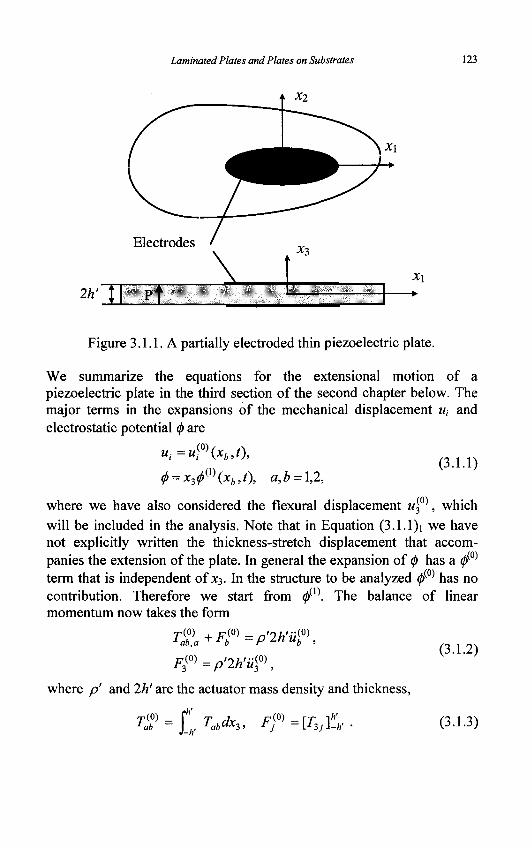
Laminated Plates and Plates on Substrates 123
2h- ::
Electrodes /
\ I i't
*3
X\
Figure 3.1.1. A partially electroded thin piezoelectric plate.
We summarize the equations for the extensional motion of a piezoelectric plate in the third section of the second chapter below. The major terms in the expansions of the mechanical displacement w, and electrostatic potential 0 are
/,(0)(**>0, • x^m(xb,t), a,b = \,2,
w, = w>
</>-. (3.1.1)
where we have also considered the flexural displacement uf^, which will be included in the analysis. Note that in Equation (3.1.1)i we have not explicitly written the thickness-stretch displacement that accompanies the extension of the plate. In general the expansion of (j) has a 0(O)
term that is independent of X3. In the structure to be analyzed 0(O) has no contribution. Therefore we start from 0(1). The balance of linear momentum now takes the form
1ab,a ^ rb
F™=p'2h'u?\.
••P'2h'ii<?\
where p' and 2h' are the actuator mass density and thickness,
Tm _ f T d 1ab - ]_ , IabaX3,
p(0) = j \T3J&
(3.1.2)
(3.1.3)
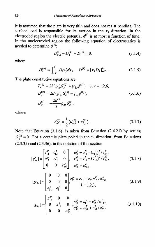
124 Mechanics of Piezoelectric Structures
It is assumed that the plate is very thin and does not resist bending. The surface load is responsible for its motion in the JC3 direction. In the electroded region the electric potential 0(1) is at most a function of time. In the unelectroded region the following equation of electrostatics is needed to determine (j>m:
D (i) •D^+Dm 0,
where
A W = £ D,x"3dx3, D^=[x,D,th,
The plate constitutive equations are
r/0)=2/>'(r;A(0)+^(1)X r,s = \,2,e,
where
A ( 0 )
Di»
= 2h'(y,i
2h'3
3
e(0) ^ab
c(0)
<;*+?
- \ ,
•Sxtm\
3
(0) , (0)x a,b + ub,a >
(3.1.4)
(3.1.5)
(3.1.6)
(3.1.7)
Note that Equation (3.1.6)3 is taken from Equation (2.4.21) by setting
SJP = 0. For a ceramic plate poled in the JC3 direction, from Equations
(2.3.35) and (2.3.36), in the notation of this section
'12
\y'n] =
WksV
[gki] =
L-12
0
0
0 0 c,
0
0
0
0
pp
e31
,p _ cE -(cE\2lcE
c l l \h3) / c 3 3 ' c i2 _ c i 2 ( C B ) ' C:
33 '
' 3 3 '
c 66=< '66 >
ei\ _ g 3 1 e33C13 ' C 3 3 '
k = 1,2,3,
0
0
0
0
FP fc33
£\\ ~ £l\ +e\5 'C44'
— £ •)-( + 633 '33 '33 . / C
(3.1.8)
(3.1.9)
(3.1.10) 33-
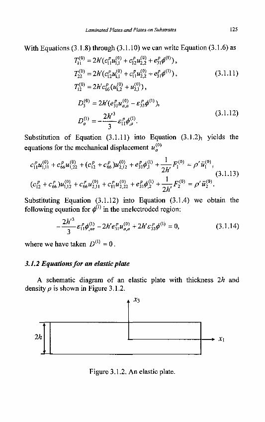
Laminated Plates and Plates on Substrates 125
With Equations (3.1.8) through (3.1.10) we can write Equation (3.1.6) as
/»„«» rPAQh D^=2h\e^a-s^),
D (i) 2h »3
PAV •*M (3.1.12)
Substitution of Equation (3.1.11) into Equation (3.1.2)i yields the
equations for the mechanical displacement w^0)
rP,A0) 4-rp?A0) + (rp + rp ~\i/0) + pp(hm +——F C\\U\,\\ + C66M1,22 + VC12 + C66>>"2,12 + ei\?,\ + Oh
1
(0) •P'u?\
(3.1.13) ;(0)
\C\2+C66)U\,\2+C66U2,\l+Cl\U2,22+ei\9,2 + ~ , , r 2 ~ P U2
Substituting Equation (3.1.12) into Equation (3.1.4) we obtain the following equation for 0(1) in the unelectroded region:
2h" •eM% -2h'ep^U2h'£&
m = 0, (3.1.14)
where we have taken Dm = 0.
3.1.2 Equations for an elastic plate
A schematic diagram of an elastic plate with thickness 2h and density p is shown in Figure 3.1.2.
A *3
2h -*• X\
Figure 3.1.2. An elastic plate.
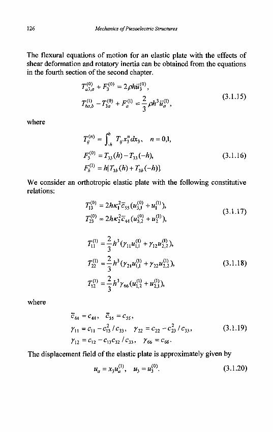
126 Mechanics of Piezoelectric Structures
The flexural equations of motion for an elastic plate with the effects of shear deformation and rotatory inertia can be obtained from the equations in the fourth section of the second chapter.
TZ-Tg+FV-lfih**?, ( 3 ' U 5 )
where
FJ0) =T33(h)-T33(-h), (3.1.16)
Fbm=h[T3b(h) + T3b(-h)\
We consider an orthotropic elastic plate with the following constitutive relations:
T$=\h\ynuV+ynu%),
(3.1.17)
T^=^h3(r2luS+r22«&\ (3-1-18)
where
c44 — C 44 ' C55 — C55 '
Y\\ =C\\ -Cu/c33, Yn =c22 -c223/c33, (3.1.19)
712 ~C\2 - C 1 3 C 3 2 'C33> ^66 = C 6 6 -
The displacement field of the elastic plate is approximately given by
ua=x3u?, «3=«30)- (3-1-20)
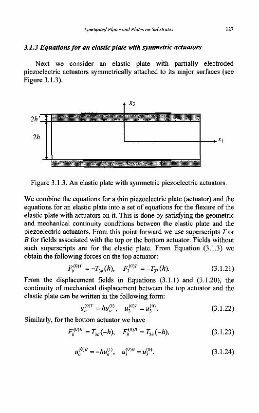
Laminated Plates and Plates on Substrates 111
3.1.3 Equations for an elastic plate with symmetric actuators
Next we consider an elastic plate with partially electroded piezoelectric actuators symmetrically attached to its major surfaces (see Figure 3.1.3).
2h'_
2h
x3
.*!
Figure 3.1.3. An elastic plate with symmetric piezoelectric actuators.
We combine the equations for a thin piezoelectric plate (actuator) and the equations for an elastic plate into a set of equations for the flexure of the elastic plate with actuators on it. This is done by satisfying the geometric and mechanical continuity conditions between the elastic plate and the piezoelectric actuators. From this point forward we use superscripts T or B for fields associated with the top or the bottom actuator. Fields without such superscripts are for the elastic plate. From Equation (3.1.3) we obtain the following forces on the top actuator:
F?)T=-T3b(h), F3mT = T33(h). (3.1.21)
From the displacement fields in Equations (3.1.1) and (3.1.20), the continuity of mechanical displacement between the top actuator and the elastic plate can be written in the following form:
(0)T = hu (i) u
(0)r _ „(0) ui
Similarly, for the bottom actuator we have
F™" =T3b(-h), F (0)8 _ T33(-h),
(3.1.22)
(3.1.23)
MB M\ u ( 0 ) * = M ( 0 ) (3.1.24)
128 Mechanics of Piezoelectric Structures
From Equations (3.1.21), (3.1.23) and (3.1.2) the equations of motion for the top and bottom actuators are
TZ-^(h) = p'2h'iir,
-T^h) = p'2h'ur,
rzB^3b(-h)=P'2h'ur, (J.1.26)
T33(-h) = p'2h'iii0)B.
For the elastic plate, from Equations (3.1.16)2>3, (3.1.25) and (3.1.26) we have
F3(0) = -p'2h'ufT -p'2h'uf)B, (3.1.27)
Fbm=KTZ -P'2h'iir -TZB+P'2h'iiri (3.1.28)
Substitution of Equations (3.1.27) and (3.1.28) into Equation (3.1.15) yields
T^=2phui0) +p'2h'u^T + p'2h'uf)B,
(TV+hTbW-hTbT\b-T^ (3.1.29)
= 2ph3uV+h[p'2h'ii«>)T -p'2h'u^B\
With the continuity conditions in Equations (3.1.22) and (3.1.24), we can write Equations (3.1.29) as
(3.1.30) f(l) _ r(0) _ K:0) V ' 1ba,b J3a ~ lua '
where f(i) _ Tm , uT(.°)T hT^B
1ba ~1ba +nlba ~nlba '
m = 2ph + 4p'h', (3.1.31)
I = -ph3 +4p'h'h2.
T^b has the clear physical meaning of total moments consisting of the
moments due to the bending of the elastic plate and the extension of
the actuators, m is the mass per unit area and / the rotatory inertia of
Laminated Plates and Plates on Substrates 129
the plate with the actuators. In the following we assume that the applied voltages on the top and bottom actuators are of equal magnitude and opposite signs and denote
^)T=_(/>mB=^)_ ( 3 1 3 2 )
Then for constitutive relations, from Equations (3.1.3l)i, (3.1.11), (3.1.18), (3.1.22) and (3.1.24) we obtain
Tg=rn»$ +W% + 4hh'e&m, (3.1.33)
where
7u = f AVii + 4h'h2cp:, yn = \h3yX2+4h'h2cp
2,
7n =\h3y12 + 4h'h2cpx, y66 = h3y66 + 4h'h2c&.
(3.1.34)
Expressions for T$ in terms of u^ and u^ are given by Equation (3.1.17). Substitution of Equations (3.1.17) and (3.1.33) into Equation (3.1.30) gives the equation for the flexural and thickness-shear motions of the whole plate including the actuators
2hK^c55 («g\ + « $ ) + Ihxlcu (w$2 + w$ ) = mu^,
ru^+rn4lx+^'he3p^
+ r66("i% +4l2)-2hK2c55{uf} + K1(1)) = /ii1
(,\ (3.1.35)
y22u{2% + ynu§2 + 4h'hep
x</>f
+ 66 ("1% +U%)-2hK2C4M°l +4)) = Iii^.
In the unelectroded portions of the actuators where ^(1) is unknown, Equation (3.1.14) is needed which now takes the following form with the use of Equation (3.1.22)i:
2h'2
-—sM% -2h'heplu^a+£
p32h'lf>
m=0. (3.1.36)
130 Mechanics of Piezoelectric Structures
At the boundary of a finite plate with a unit normal na and a unit tangent
sb we need to prescribe
naT^nb or « B \ ,
nai$>sb or i/»5fl, (3.1.37)
T$> or „<»>.
For electric boundary conditions we need to prescribe
«„Z)B0) or $>(1). (3.1.38)
Although the equations derived in this section include shear deformation and rotatory inertia and can be used in situations when the elastic plate is not very thin, the piezoelectric actuators are still assumed to be very thin compared to the elastic plate and are treated as thin films that are in extensional motions and do not resist bending.
3.1.4 Reduction to classical flexure
When the elastic plate is very thin, the effect of shear deformation and rotatory inertia can be neglected. Equations for this case were given in [37], and can be reduced from the equations derived above. For thin plates we neglect shear deformation and rotatory inertia, which results in
7 = 0, i ^ - t t j 0 ; . (3.1.39)
Then, similar to the reduction in the fourth section of the second chapter, Equation (3.1.33) and Equations (3.1.35) through (3.1.37) reduce to
iff =-yii«£?i -rn«i% +4h'he^l\
T^=-rn«i% -722^2 +4h'he(Jm, (3.1.40)
7 12 _ i 2 1 "" z / 6 6 " 3 , 1 2 '
fd) __£ u(0) _2(y +7Y W0 ) -v w(0)
1ab,ab- /11M3,1111 Z V 1 2 + Z / 6 6 JM3,1122 /22M3,2222
+ 4h'hefiW§ + +%) = miif\ (3.1.41)
- ^ s ^ % +2h'he&Z +2h'e&V = 0,
Laminated Plates and Plates on Substrates 131
where
.(1) ^ (3-1.42)
r ^ + % - or Mf,
? ; (3
0 )=7S, f « = n f l f ( g) j i . (3.1.43)
5.7.5 Dispersion relations
To see the difference between Equation (3.1.35) and Equation (3.1.41)], we consider the one-dimensional case of fully electroded actuators with shorted electrodes. Then
i41} = 0, ^(1) = 0, <?2=0. (3.1.44)
From Equation (3.1.41) we obtain
-rn«l%n=™i0)- (3-1.45)
The substitution of the wave solution uf^ =exp/'($c, - cot) into Equation (3.1.45) leads to the following dispersion relation for flexural waves:
fi>2=%£4. (3.1.46) m
Under Equation (3.1.44), from Equation (3.1.35) we have
2hK2c55{uf}x+u^) = rhuf\
ynu[l-2hKtc55(u?l+uV) = iu?\
Consider the following waves:
ui0) -Aexpi(&cx - cot), PK^ (3.1.48)
u\' = Bexpi(^xx - cot).
Substitution of Equation (3.1.48) into Equation (3.1.47) results in
2hK,2c55 {-£,2A + i£B) = -mco2 A, „ (3.1.49)
- fn^B - 2hK2c55 (i$4 + B) = -Ico2B,
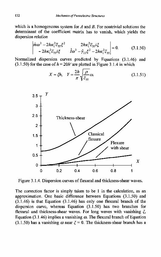
132 Mechanics of Piezoelectric Structures
which is a homogeneous system for A and B. For nontrivial solutions the determinant of the coefficient matrix has to vanish, which yields the dispersion relation
-2 -2hic?c5542
ma) 2hrcx c55i^
•2hK?c„it I<D2-yne • 2hic12c55
0. (3.1.50)
Normalized dispersion curves predicted by Equations (3.1.46) and (3.1.50) for the case ofh = 20h' are plotted in Figure 3.1.4 in which
(3.1.51)
X
0.2 0.4 0.6 0.8
Figure 3.1.4. Dispersion curves of flexural and thickness-shear waves.
The correction factor is simply taken to be 1 in the calculation, as an approximation. One basic difference between Equations (3.1.50) and (3.1.46) is that Equation (3.1.46) has only one flexural branch of the dispersion curve, whereas Equation (3.1.50) has two branches for flexural and thickness-shear waves. For long waves with vanishing £ Equation (3.1.46) implies a vanishing 0). The flexural branch of Equation (3.1.50) has a vanishing a> near £ = 0. The thickness-shear branch has a
Laminated Plates and Plates on Substrates 133
finite cutoff frequency at £ = 0. For flexural motions, Equation (3.1.46) and the flexural branch of Equation (3.1.50) agree only for very small values of £h. Since in the flexural problem of a finite plate the wave number £ is of the order of the inverse of the dimension L of the plate, Equation (3.1.46) is valid only for plates with small values of h/L, or very thin plates. When h/L is not very small, the equations with thickness-shear deformation and rotatory inertia should be used.
3.2 Elastic Plates with Piezoelectric Actuators on One Side
In some applications an elastic plate carries a piezoelectric layer only on one side, either as an actuator or a sensor. In this case the structure is sometimes called a unimorph. For unimorphs, due to the asymmetry about the middle plane of the structure, bending and extension of the middle plane are inherently coupled. This causes complications in modeling. In this section we derive two-dimensional equations for a plate piezoelectric unimorph and use the equations obtained to analyze circular disk unimorphs [39]. A unimorph is a special case of laminated plates. Two-dimensional equations for laminated piezoelectric plates can be obtained by combining equations for each layer like in the previous section. They can also be obtained directly by substituting approximate expressions of the global displacement and potential fields into the variational formulation. In the variational approach, since a laminated plate is a body with piecewise constant material parameters that do not have derivatives across an interface, the integrations in the variational formulation have to be performed layer by layer. Interface continuity conditions on traction and electric displacement are part of the stationary conditions of the variational procedure. These conditions can be satisfied exactly by three-dimensional solutions, or approximately by two-dimensional solutions. Another approach for developing equations of single-layered or laminated plates is to calculate moments of various orders of the three-dimensional equations and fields by integrating them through the plate thickness [40,41]. This is the approach we follow in this section.
3.2.1 Classical theory
Consider the two-layer plate in Figure 3.2.1, which is asymmetric about its middle surface.
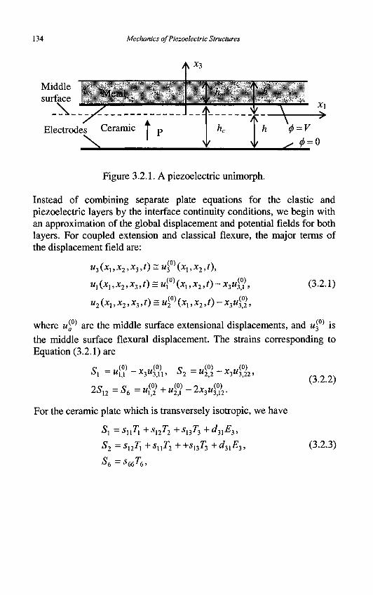
134 Mechanics of Piezoelectric Structures
A *3
Middle surface Molal
.\.^Z Electrodes Ceramic f p \ L
A h.
r > = K
^ <* = 0
Figure 3.2.1. A piezoelectric unimorph.
Instead of combining separate plate equations for the elastic and piezoelectric layers by the interface continuity conditions, we begin with an approximation of the global displacement and potential fields for both layers. For coupled extension and classical flexure, the major terms of the displacement field are:
"*3 \X\ J %2 ' "*"3 ' / = ^3 \X\,X2,t),
u](x1,x2,x3,t) = u<i0)(x1,x2,t)-x3u^, (3.2.1)
where w£0) are the middle surface extensional displacements, and «<0) is the middle surface flexural displacement. The strains corresponding to Equation (3.2.1) are
c _,.(o) • r M ( 0 ) <7 - u m - x M ( 0 )
•*3"3,11 ' ° 2 — M2,2 -*3"3 ,22 '
j«2 — O^ — ^ 1 2 ^ 2 1 £*X\U'i
(3.2.2) 2o! - ) — o f i — « i 9 -r « ? 1 - i" ,-3"3J12 •
For the ceramic plate which is transversely isotropic, we have
" 1 = ^ll-M + SU*2 "*" SV>^ + " 3 1 ^ 3 '
2 _ ^ H ^ l + 5 11^2 + + 1 $ 1 3 ^ 3 + " 3 1 - ^ 3 '
" 6 = 5 66^6>
(3.2.3)
Laminated Plates and Plates on Substrates 135
where s66 = 2(sn-si2) and £3 = -V/hc. For a thin plate we make the stress relaxation
T3 = 0. (3.2.4)
Under Equation (3.2.4), Equation (3.2.3) can be inverted to give
'\ = C 1 1 " 1 + C 1 2 0 2 — e31-^3>
T2^cxp2Sx+cx
pxS2-e^E3, (3.2.5)
^12 ~ C 6 6 ^ 6 '
where
: 5 U / A , c,^ = - 5 1 2 / A , A = sj2, - 5 ^ (3.2.6)
(3.2.7)
>12>
«31 = ^ 3 1 /(*11 +Sl2), Cl =1/S66 = (c[x -c[2)/2.
Then the relevant electric constitutive relation takes the form
D3 = d3X(Tx+T2) + e33E3
= e3p
x(Sx+S2) + £f3E3,
where
^ 3 = ^ 3 3 - 2 ^ 3 1 . (3.2.8)
Equation (3.2.7) is useful when the charge or current on the electrodes at the major surfaces of the ceramic plate needs to be calculated.
For the elastic metal layer that is isotropic, we use a hat to indicate its material parameters. Using a method similar to the derivation of Equation (3.2.5), we have
7, =c11i>1 +cl2S2,
T2=cxp
2Sx+cfxS2, (3.2.9)
^12 = C 6 6 " ^ 6 '
where
C l l ~ s\l ' &> c\2 ~ ^ 1 2 ' A , A —Jj[ SX2,
cp6=l/s66=(cp
x-cp
2)/2. (3.2.10)
136 Mechanics of Piezoelectric Structures
With Equations (3.2.5) and (3.2.9), we calculate the plate extensional resultants as
Tjf = lTndx,
- a i/0) + a »y(0) + h w ( 0 ) 4- h w ( 0 ) - h op F - " l l " l , l + " 1 2 " 2 , 2 + 0 l l "3 , l l + °12M3,22 "ce3l£'3>
l h ( 3 . 2 . 1 1 )
- a u(0)+a u(0)+h w ( 0 ) +b w ( 0 ) - h e p E _ " l 2 " l , l + " l l " 2 , 2 + °12"3,11 + 0 l l"3,22 " c ^ l " ^ '
*12 — J ^ ^ n ^
where
_ "66 l " l , 2 + "2,1 / + Z°66"3,12 '
fli i = cu Ac + Cu K, al2 = c[2 hc + c& hm,
«66 = C 6 6 ^ c +C«,K = («11 - « 1 2 ) / 2 '
*.l =|(<1 - ^ > A > .2 =|fcP2 ~ ^ K * U . (3-2"12)
b66=\(c£6-£g6)hchm=(bu-bl2)/2.
In obtaining Equation (3.2.11) we have made the usual approximation that in the thin ceramic layer the electric field E3 is essentially independent of JC3 [3]. Similarly, the plate bending and twisting moments are given by
7j, = y^T^^dx^
- _ / , ,/°)_A M(°)_v w(0) - v M(0) + / I / I P P F - °11"1,1 °12"2,2 / l l " 3 , l l /12M3,22 +"c"»i e31- c ' 3>
r22 = J_ ^22*3^3
- _A M(°) _ A „(°) _ v M(°) _ y u ( ° ) + / , /, eP F - °12"l,l °11M2,2 /12"3,11 /U"3,22 + " e " m e 3 1 £ , 3 '
- - / > f M ( 0 ) + w ( 0 ) s > - 2 v M ( 0 )
_ °66 V"l,2 + "2,1 J z / 6 6 " 3 , 1 2 '
(3.2.13)
Laminated Plates and Plates on Substrates 137
where
rn = cA(hi+3hx)+^(hi+3hX]
, p / \ zp
Yn = ^ - f e + 3 A c ^ ) + ^ - f c +3hX\ (3-2-14)
r66 = ^ f f e + 3 ^ ) + ^ - f c +3h?hm)=(ru -Yn)l2.
For the plate equations of motion for extension and flexure, instead of using the variational principle, we integrate the three-dimensional equations of motion through the plate thickness
?Z +\Tibth =(Pchc+PmhmWl0) +\iPc -Pm)hchmuf}, 2
TZ+\T*th={PcK+pmK)u?)-
The second term on the right hand side of Equation (3.2.15)j is in fact
due to the first-order displacement and is usually smaller
than the first term because it depends on the difference of the mass densities and it has a spatial derivative. The classical theory for flexure is for long waves with small wave numbers. A spatial derivative is effectively a multiplication by the small wave number. The plate moment equations are obtained by integrating the product of the three-dimensional equations of motion and x^ through the plate thickness. This
gives the plate transverse shear resultants TJ^ in terms of the moment resultants
TZ - 4 0 ) + M J - * = -\iPc -pm)KK*T • (3-2.16)
In Equation (3.2.16) the rotatory inertia has been neglected for classical flexure. The surface load in this equation is neglected below.
In summary, we have the two-dimensional equations of extension and flexure (3.2.15), constitutive relations (3.2.11) and (3.2.13), shear force-moment relation (3.2.16), and strain-displacement relations (3.2.2). With successive substitutions, Equation (3.2.15) can be written as the
following equations for uf^, uf^, and w^ :
138 Mechanics of Piezoelectric Structures
066vVo) +^^v(vV(Vz>nv(v2Mf)
h -Ke^VE.+lT^+T^]
= {pchc + Pmhm)ui0)+^pc-pm)hchmM0), (3-2.17)
-r„v2v2Mf -^v 2 (v .« (»V^A + [r33fft
= ( p A + A A ) ^ ~\{Pc -Pm)hchmV-n{«\
where u(0)=Ml
(0)i1 + 40 ) i2 , (3.2.18)
V = i,a1+i252 , V=d\+d\.
At the two-dimensional boundary of a plate with an in-plane unit exterior normal n and an in-plane unit tangent s, we may prescribe
r ( 0 ) or w(0) Tm or w(0)
r(0 . rd) o r M(0) r ( D o r M ( ° ) V • • J i«3 +1ns,s OT " 3 ' ^ n OT "3,n •
3.2.2 Stress function formulation for static problems
For static problems, it is often convenient to use a stress function for
the extensional part of the problem. Consider the case of [T3b ~\h_h = 0.
The static form of Equation (3.2.15)i becomes
7 ^ = 0 , (3.2.20)
which can be identically satisfied by the introduction of a stress function yj through
Z i f ^ . 2 2 , TM=yM, r1 20 )=-^> 1 2 . (3.2.21)
Then, from Equation (3.2.11)
i// - n um+n M ( 0 ) + / > w ( 0 ) + A w ( 0 ) -hepF
V\22 _ " l l " l , l +"12"2 ,2 + ° l l " 3 , l l + °12"3,22 " c ^ l " ^ '
V.n = «i2«i(? +*ii"w +ii2"30n + *ii«$2 - W i ^ s . (3-2-22)
- ^ 1 2 = « 6 6 ( " I( 0 2 ) + ^ 1 ) ) + 2 6 6 6 < 1
)2 -
Laminated Plates and Plates on Substrates 139
Equation (3.2.22) can be inverted for
"1,1 ~ ^ 2 ^ , 1 1 2 2 ^ , 2 2 « 1 1 - « 1 2 « 1 1 - « 1 2
fllAl ~ a 1 2 ^ 1 2 , , (0) « n ^ i 2 ~ Q l 2 ^ U „ ( 0 ) , ^ c g 3 1 F 2 2 3,11 2 2 3,22 "*" ^ 3 >
a n -a 1 2 «i i-«n an+«i2 (0) _ a l l . . . Q12
"2 ,2 _ 2 2 ^ . 1 1 2 2 ^ , 2 2 «n-«i2 on-al2
aubn -anbu _(0) OiAi~fi2*i2 „(o) , ^ce3i F 2 2 3,11 7 2 3,22 i~ c 3 '
« 1 1 - « 1 2 « 1 1 - « 1 2 « 1 1 + « 1 2
„(«)+„«») =_J_„„_2A66.1|(0)
(3.2.23)
1,2 + M2,1 _ ^ , 1 2 M3,12 " 6 6
2{bn-bn) (0) y \12 "3,12 •
a l l ~ a 1 2 a l l - « 1 2
Substituting Equation (3.2.23) into the following compatibility equation:
("l(,?),22 + («$),11 = («U + "2°,}),12 , (3-2.24)
we obtain
" i i V V - ^ i W f + ^ V2E3 = 0 , (3.2.25) « U + « 1 2
where
a n = — ~» 6u = 2 2 • (3.2.26) an-an au-an
Substitution of Equation (3.2.23) into the moment expressions in Equation (3.2.13) gives
TlP =-rn4% -fl2«3°22 -^1^,11 -bn¥,22+KKe^,
T£)=-ri2«i% -rn"i% -bx2V,n -bu¥,22+KK^E„ (3.2.27)
•M2 = — 2 ^ 6 6 M 3 1 2 — b66i//u,
140 Mechanics of Piezoelectric Structures
where
- _v au(bu+bi2)-2aububn
I\\ -J\\ 2 2 a\\
2anbnbn-}\2-/n 2 an
r a i 2 * i 2 - a i A i °\2 ~ 2 2 '
an-an
-an
an(bu 2
-au
~bn)2
ba =
+ bu) ?
K=hm
* l l - ^ 2
au-an
bU +^12
au+an
(3.2.28)
Then Equation (3.2.15)2 takes the following form:
- f „ V 4W f -bnV
4¥ + hmhce^2E, +[T,3lh = 0. (3.2.29)
In this stress function formulation the equations that govern if/ and wf
are Equations (3.2.25) and (3.2.29).
3.2.3 A circular plate under a uniform load
As an example we consider circular plates under axi-symmetric loads. For axi-symmetric problems in polar coordinates, we have
„4 d4 2 53 1 d2 Id V = — r + r-^r—r + -dr4 r 8r3 r2 dr2 r3 dr '
T(U> = • n(0) _ 1 dy_
r dr
T® = -TnuZ J-^uf) -buY,rr - % , + W ^ , (3-2.30) r r
r0) -_Zk, , (°) -v w(0) - -^ - i / / -A i// +h hpp F Iee M3,r /12"3,/r ¥ ,r °\2¥,rr+nmncenL/3'
r r j(0) _01rr Lrr 2 80
dr r
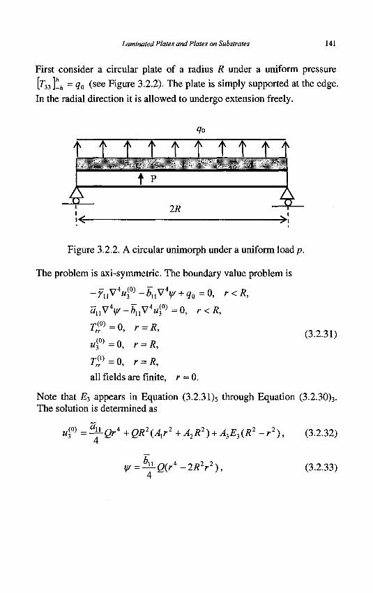
Laminated Plates and Plates on Substrates 141
First consider a circular plate of a radius R under a uniform pressure
[r33 ]h_h = <70 (see Figure 3.2.2). The plate is simply supported at the edge.
In the radial direction it is allowed to undergo extension freely.
S, A A A
t P
t Qo
A t t A A
£ • < -
2R £
(3.2.31)
Figure 3.2.2. A circular unimorph under a uniform load p.
The problem is axi-symmetric. The boundary value problem is
-ynV4uf)-bnV
4¥ + qo=0, r<R,
auV*p-bnV440) = 0, r<R,
Tr{P=0, r = R,
M(°) =0, r = i?,
7^=0, r = J R ,
all fields are finite, r = 0.
Note that £3 appears in Equation (3.2.31)5 through Equation (3.2.30)3. The solution is determined as
M(0) = ?lLQr*+QR2(Alr2+A2R
2) + A3E3(R2 -r2), (3.2.32)
An yr=-U-Q(r*-2Rir'), 4
(3.2.33)
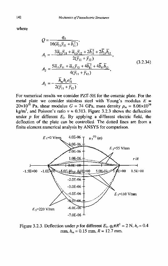
142 Mechanics of Piezoelectric Structures
where
e=—r 9o
1 6 ( 0 , ^ , ! + ^ )
_ 3aiiFn + ajifi2 + 2 5 i + 2 V12
2(Fn+Fi2)
5«iiFn + «nFi2 + 4^ii + 4*1 A 2
(3.2.34)
^ 2 =
4="
4(rn +r i 2 )
2(Fll+Fl2) '
For numerical results we consider PZT-5H for the ceramic plate. For the metal plate we consider stainless steel with Young's modulus E = 20x10'° Pa, shear modulus G = 74 GPa, mass density pm = 8.06xl010
kg/m3, and Poisson's ratio v = 0.313. Figure 3.2.3 shows the deflection under p for different £3. By applying a different electric field, the deflection of the plate can be controlled. The dotted lines are from a finite element numerical analysis by ANSYS for comparison.
£3=0V/i
£3=55 V/mm
-1.5E+00 -1.0E\00^-5JQ!
£3=220 V/mm
rlR
S.OSr.Oi^l.VE+OO 1.5E+00
/ / £3=110 V/mm
Figure 3.2.3. Deflection underp for different E3. q0irR2 = 2 N, hc= 0.4 mm, hm = 0.15 mm, R - 12.7 mm.
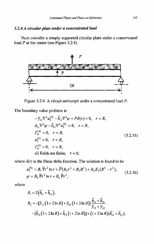
Laminated Plates and Plates on Substrates 143
3.2.4 A circular plate under a concentrated load
Next consider a simply supported circular plate under a concentrated load P at the center (see Figure 3.2.4).
£ <<-
t t P
27? £ Figure 3.2.4. A circuit unimorph under a concentrated load P.
The boundary value problem is
a n V V - * i i V 4 « l 0 ) = 0 , r<R,
7 l 0 ) =0 , r = tf,
,(») = 0, r = R, (3.2.35)
7 ^ = 0 , r = R,
all fields are finite, r = 0,
where $>) is the Dirac delta function. The solution is found to be
uf) = Bx Pr2 Inr + P(B2r2 + B3R
2) + B4E3 (R2 - r2 ),
^ = £ 5 Pr 2 l n r + 56Pr2 (3.2.36)
where
Bl=2(bli+bl2),
B2=-[ru{3 + 2]nR) + yi2(l + 2]nR)]bi^ + bn
Yu+Tn
-\bu(l + 2\nR) + bn{\ + 2hiR)\ + (\ + 2\nR)(bn+bn),
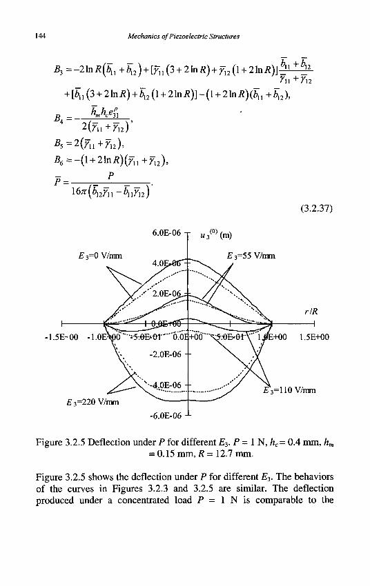
144 Mechanics of Piezoelectric Structures
B3 = -2lnR(bn + ^ 2 ) + [fu(3 + 21n^) + f12(l + 21nJ?) ]^ 1 + ^ 2
+ [^1(3 + 21ntf) + 2 ( l + 21n/?)]-(l + 2h7?)(^ 1 +6 n ) ,
B KKel\ 2(Fn+Fi2) '
^s=2(7n+yi2). 5 6 = - ( l + 21n/?)(7u+712),
P- P
I6n(bnyu-buyn)
(3.2.37)
£3=OV/mm
6.0E-06T M3TO(m)
£3=55 V/mm
-1.5E+00 -1 .OE PO '•--5-.eE'Or 0.
-2.0E-06
.-OB-Oi'V lJlE+00 1.5E+00
£VH0V/mm £3=220 V/mm
-6.0E-06
Figure 3.2.5 Deflection under P for different E3. P = 1 N, hc= 0.4 mm, hm
= 0.15 mm, R = 12.7 mm.
Figure 3.2.5 shows the deflection under P for different £3. The behaviors of the curves in Figures 3.2.3 and 3.2.5 are similar. The deflection produced under a concentrated load P = 1 N is comparable to the
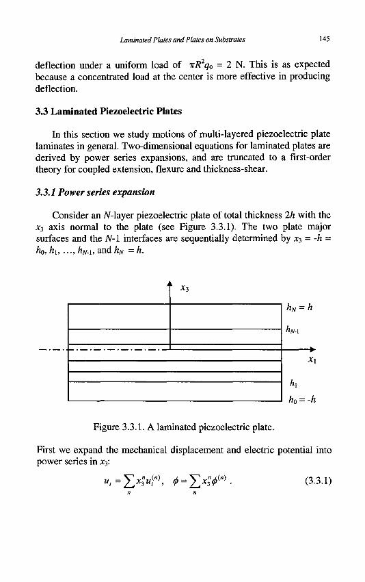
Laminated Plates and Plates on Substrates 145
deflection under a uniform load of irR2q0 = 2 N. This is as expected because a concentrated load at the center is more effective in producing deflection.
3.3 Laminated Piezoelectric Plates
In this section we study motions of multi-layered piezoelectric plate laminates in general. Two-dimensional equations for laminated plates are derived by power series expansions, and are truncated to a first-order theory for coupled extension, flexure and thickness-shear.
3.3.1 Power series expansion
Consider an Af-layer piezoelectric plate of total thickness 2h with the x3 axis normal to the plate (see Figure 3.3.1). The two plate major surfaces and the N-l interfaces are sequentially determined by x^ = -h = ho, hi, ..., hN.\, and hN = h.
4- »-
I hN = h
1 ». Xi
hi
1 h0 = -h
Figure 3.3.1. A laminated piezoelectric plate.
First we expand the mechanical displacement and electric potential into power series in X3:
K,=5>3"«<"\ ^=2> 3 y> . (3.3.D
146 Mechanics of Piezoelectric Structures
Then
S9=^Sf\ E,=^E}"K (3.3.2) n n
where
siH) 4 [M^+u%+(»+ix* f l«r}+v^ , }>]. (3 3 3) £ w = - ^ " ) - ( „ + i ) ^ 3 . ^ " + i ) .
For the two-dimensional equations of motion and charge, we multiply
TjtJ=pu„ D„=0 (3.3.4)
by x", integrate the resulting equations across the thickness of the /-th
layer from /t/.i to hi, sum over /, and make use of the interface continuity conditions of the traction vector and the normal component of the electric displacement. We then obtain the following n-th order field equations
Tv"t -nTJJ-l)+FJn) ^p^^iifK (3.3.5)
D$ -nD^ +DW =0,
where
{7j">, A(n)} = lh {Ty , D, }x"3dx3 = X £ {Tv , D, }x"3dx3,
Ff] =[x»3T3Jth, /)<"> = [x"3D3 f_h, (3-3.6)
Substitution of the three-dimensional constitutive relations of the 7-th layer
Tij = cijkiSki ~ ekijEk >
D^eJuSu+s'gEj
Laminated Plates and Plates on Substrates 147
into Equation (3.3.6)! gives the plate constitutive equations of order n as follows
1ij ~ / \ciikl °kl ekij ^k h m
^ )=E(C ,^ )-4"+" )£/ f f l ))> (3.3.8)
where
(3.3.9)
7=1 '"'-1
g*y = 2-1 L ekijX3X3 "Xi> 7=1 h/-'
7=1 * ' - '
3.3.2 First-order theory
For a first-order plate theory of coupled extensional, flexural and thickness-shear motions we make the following truncation of Equation (3.3.1):
M, =uf){xx,x2,t) + xiuf\xx,x2,t) + xlu\2){xx,x2,t),
A<°> </) = <t)K >(x1,x2,t) + x30(>(xl,x2,t), 0)/
(3.3.10)
where u^ and wj2) will be eliminated by stress relaxations. The strains
and electric fields are
Sp=Sf+X3Sf, p = l,2,-,6, 7(0)
E.sEr+x,^1, ?m (3.3.11)
where the zero- and first-order strains are
c ( 0 ) _ „ ( 0 ) o(0) _ (0) o (0) _ (1) 1 — 1 1 ' 2 — 2 2 ' 3 — " 3 '
5 , r = « i 2 , + « 2 , 5 ^ = 1 / ^ + 1 1
*2,2'
(0) _ „ (0) / I ) 5<°>= i i ^ + i i (0) (3.3.12)
148 Mechanics of Piezoelectric Structures
and
S2)=u^+2ui0)=0, S®=u®+2u{2)=0, (3.3.13)
cO) _ ,,(1) , M(l)
We note that S^ and S® are involved with u^ and w^2), which are to
be eliminated. S^ and S^ are neglected as an approximation. The zero- and first-order electric fields are given by
^ ( 0 ) = - ^ j 0 ) . E^=-<l>f, Ei0)=-*m, (3.3.14)
and
E^=-cj>f, E?=-j$\ E®=0. (3.3.15)
The zero- and first-order equations of motion and charge are
TZ +FF =±P'[{h1 -h,_xyuf> + 4 b * k ««], 7=1 L
7=1
TZ -T^+F^=±p'[^^-u^ + ^ l * M . f i « ] , (3.3.16)
Z>2+Z)(0)=0,
DS-A ( 0 )+^ ( 1 )=O.
The zero-order plate constitutive relations are
D™ =(e$Sf +e<?E<P ) + ($*« +sfEf), (3.3.17)
Laminated Plates and Plates on Substrates 149
where
I=\
1=1
and
JL h1 -h2 " h2 -h1
(1) _ y ,*I "i-l y-I (1) _ Y ("' " ^ \F'
7=1 Z 7=1 Z
N h2 h2
7=1 L
The first-order constitutive relations are
D^=(epf+e^Ef) + (e^+e^E<P),
where
N U3 U3 N U3 U3
(2) _ Y (hzhzLXr1 e
(2) - Y C1 ~ '~l)c!
ijkl - Z - A I ' 'M' k'J ~ Z-i^ -> ' k'J'-7=1 J 7=1 J
(3.3.18)
(3.3.19)
(3.3.20)
(3.3.21)
Note that in Equations (3.3.18), (3.3.19) and (3.3.21) we have used the following material constants after the simpler version of stress relaxation (see Equations (2.4.13) through (2.4.15)):
c1 - r ' - c 1 c' lr' cijkl - cijkl t//33c"33£/ ' c3333 >
ekij~ekij ek33C33ij 'C3333' ( 3 . 3 . 2 2 )
<' e1 I c 1
<33ej33 ' c3333 • En — £„ + £ /T>£ .•« /
Then u^ and u'tp will not appear in the constitutive relations in
Equations (3.3.17) and (3.3.20). A more sophisticated stress relaxation
150 Mechanics of Piezoelectric Structures
using r3(30) = 0 and Tff = 0 to eliminate S^> and SfJ (and hence w<1}
and uf) can be performed. Two shear correction factors K\ and K2 can
be introduced by replacing the following zero-order strains:
^31 ~* K\^i\ » ^32 — > K2^ii (3.3.23)
to correct the two fundamental thickness-shear resonant frequencies. In summary, we have the two-dimensional equations of motion and
charge (3.3.16), constitutive relations (3.3.17) and (3.3.20), and strains and electric fields (3.3.12) through (3.3.15). With successive
substitutions, seven equations for uf^, u^, 0(O) and 0(1) can be obtained. At the boundary of a plate with an in-plane unit exterior normal n and an in-plane unit tangent s, we may prescribe
*£0) or «<°\ rW or u?\ T^ or uf\
r « or „ « , T® or „ « , (3.3.24)
D™ or ^ \ D™ or </>m.
For a laminated plate, extension and flexure are usually coupled unless the plate is laminated symmetrically about its middle surface.
3.4 A Plate on a Substrate
A thin film on the surface of a half-space or at the interface between two half-spaces is a common structure in device applications. In this case, for long waves, the film can be modeled by the two-dimensional equations [42], and the half-space(s) by the three-dimensional equations. In this section we analyze two problems of this type.
3.4.1 A Piezoelectric film on an elastic half-space
First consider a piezoelectric film on an elastic half-space (see Figure 3.4.1) [43]. This problem is useful for understanding the behavior of piezoelectric actuators. The film is modeled by the equations for the extensional deformation of thin plates, and the substrate is governed by the equations of elasticity. The film is of ceramics with thickness poling, and is partially electroded. The thick lines represent electrodes. The substrate is isotropic.
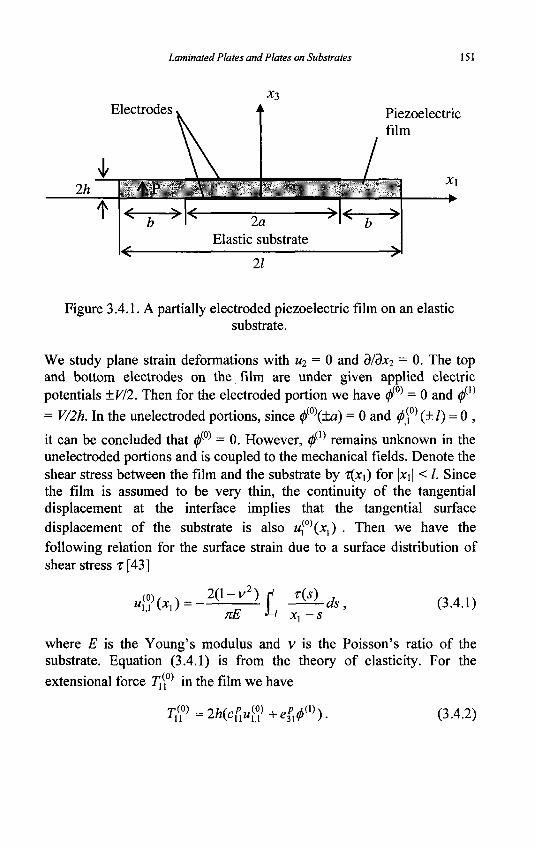
Laminated Plates and Plates on Substrates 151
*3 Electrodes
2h /fvp
Piezoelectric film
X\
-H< la Elastic substrate
• > < -
21
Figure 3.4.1. A partially electroded piezoelectric film on an elastic substrate.
We study plane strain deformations with Ui = 0 and d/dx2 = 0. The top and bottom electrodes on the film are under given applied electric potentials ±V/2. Then for the electroded portion we have 0(o) = 0 and 0(1)
= V/2h. In the unelectroded portions, since 0(O)(±a) = 0 and ^ j 0 ) (± /) = 0 ,
it can be concluded that 0(o) = 0. However, 0(1) remains unknown in the unelectroded portions and is coupled to the mechanical fields. Denote the shear stress between the film and the substrate by T(X]) for \x\\ < I. Since the film is assumed to be very thin, the continuity of the tangential displacement at the interface implies that the tangential surface displacement of the substrate is also wf'Oe,) . Then we have the following relation for the surface strain due to a surface distribution of shear stress T [ 4 3 ]
"I(.I)(X1) = -2(1- v2)
7lE r, T(S) ds (3.4.1)
where E is the Young's modulus and v is the Poisson's ratio of the substrate. Equation (3.4.1) is from the theory of elasticity. For the
in the film we have extensional force Tfp
TW-TKc&W+e&V). (3.4.2)
152 Mechanics of Piezoelectric Structures
7j, must satisfy the following edge conditions
ri(,0)(±0 = 0. (3.4.3)
The equation of motion of the film is
r = 7 $ . (3.4.4)
Integrating Equation (3.4.4) from -/ to JCI, using Equation (3.4.3), we obtain
\X'ir{s)ds = T^\xx). (3.4.5)
Substituting Equation (3.4.1) into Equation (3.4.2) and the resulting expression into Equation (3.4.5), we have the following integral equation for T:
2hc(x2{\-v2) ri T(S) n . . , 2hc(x2{\-v') ri r(s)ds + —- - ds
TJE J-/ xx-s (3.4.6)
= 2he?x<f>m(xx), \xx\<l.
For the electric potential we have
m [V I2h, I x, |< a, <j>m = \ i l l ' ( 3 _ 4 7 )
[unknown, a <\ xx \<l,
where 0(1) in the unelectroded portions is part of the unknowns and has to be obtained by solving simultaneous equations. The additional equation for determining (j)m takes the following form with the substitution of Equation (3.4.1) into Equation (3.1.14) and ^'replaced by h:
2^ 2he^2(l-v') e' r{s) I -ds KE • I " (3.4.8)
91,3
- —expx<l>fx - 2hsy{X), a <| x, |< /,
which is coupled to %. Equation (3.4.8) is an integro-differential equation to which we need to impose the following boundary conditions:
f\±d) = VI2h, $\±l) = 0. (3.4.9)
Laminated Plates and Plates on Substrates 153
We have obtained a pair of coupled integro-differential equations (3.4.6) and (3.4.8) for determining t(x\) and <j)m(x{), with boundary conditions (3.4.9). Equation (3.4.8) is over the region of the unelectroded portions of the film only, where (j)m is unknown.
3.4.1.1 Rigid substrate
First consider the special case of a fully electroded film on a rigid
substrate. We have w,(0) = 0. Because of symmetry we only consider half
of the film with 0 < JCI < /. For a fully electroded film with a = I, we have
0m=V /2h over the whole film. Equation (3.4.2) then implies that the
film extensional force T^ has a constant value of e-f, V along the film.
Then Equation (3.4.4) further implies that the shear stress T is zero under
the film. However, Equation (3.4.3) requires that 7j(,0) must vanish at
both ends of the film. This is possible only when two concentrated shear
forces of equal magnitude e%x V and opposite in direction are present at both ends of the film. Mathematically, the shear stress distribution can be represented by
t{xx) = -e!;xV[8{xx -l)-S(xx + /)] , (3.4.10)
where 8(xx) is the Dirac delta function. A slightly more general case is when a partially electroded film is on
a rigid substrate. In this case from Equations (3.4.6) and (3.4.8) we have
2h3 (3.4.11)
for which the boundary conditions in Equation (3.4.9) still apply. From Equation (3.4.11)2 and Equation (3.4.9), the following solution for 0(I)
can be obtained
,m f V/2h, 0<xx <a, <j)() =\ (3.4.12)
[G exp[-^(xx - a)] + H exp[£(x, - a)], a<xx<l,
154 Mechanics of Piezoelectric Structures
where
, 2 3 i c V h\ eft' 2h[l + exp(-2^b)Y
(3.4.13)
H-2/?[l + exp(-2#>)
exp(-2£Z>),
and b = l-a. Substitution of Equation (3.4.12) into Equation (3.4.1 l)i gives the shear stress distribution
t-<
0, 0 < xx <a,
<& {-exp[-£(*, -a] 1 + exp(-2#>)
+ exp(-2£fr)exp[£(jt, -a]}, a<xx<l.
(3.4.14)
Under the electroded portion there is no shear stress. In the unelectroded portion the shear stress decays exponentially with i(0 = 0- The important difference between Equations (3.4.14) and (3.4.10) is that one predicts a distribution of finite shear stresses while the other has a singular distribution of the delta function. This shows the advantage of partially electroded actuators in reducing stress concentration. The total shear force predicted by Equation (3.4.14) can be obtained by integrating the shear stress over the unelectroded region (a, /), which yields
Q = e$xV
1 + exp(-2#>) [-1 + 2exp(-#>) - exp(-2#>)]. (3.4.15)
For the equations of a thin film to be valid in the unelectroded portion, the length of the unelectroded portion b has to be much larger than the thickness 2h. Then it can be seen from Equation (3.4.13)i that in this case e x p ( - ^ i ) « 1. If we neglect exp(-<f#) compared to one in the above
expressions, we obtain the following simpler and physically more revealing expressions:
i(D Pl> = VI2h, 0 < xx <a,
2h exp[-^(x, - a)], a<xx <l,
(3.4.16)
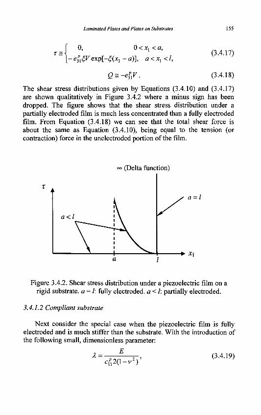
Laminated Plates and Plates on Substrates 155
T = < o, 0 < JCj < a,
• ef,i;V exp[-£(jtj - a)], a < xx < I, (3.4.17)
Q = -efiV. (3.4.18)
The shear stress distributions given by Equations (3.4.10) and (3.4.17) are shown qualitatively in Figure 3.4.2 where a minus sign has been dropped. The figure shows that the shear stress distribution under a partially electroded film is much less concentrated than a fully electroded film. From Equation (3.4.18) we can see that the total shear force is about the same as Equation (3.4.10), being equal to the tension (or contraction) force in the unelectroded portion of the film.
(Delta function)
a = I
Figure 3.4.2. Shear stress distribution under a piezoelectric film on a rigid substrate, a = I: fully electroded. a < I: partially electroded.
3.4.1.2 Compliant substrate
Next consider the special case when the piezoelectric film is fully electroded and is much stiffer than the substrate. With the introduction of the following small, dimensionless parameter:
A= „ E , , (3.4.19) cf,2(l-v2)
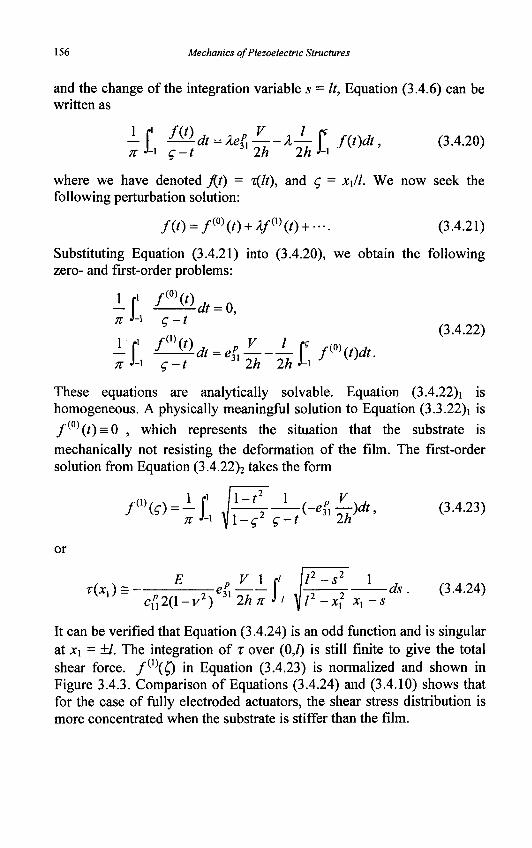
156 Mechanics of Piezoelectric Structures
and the change of the integration variable s = It, Equation (3.4.6) can be written as
-f —dt = Wx?--X±-¥ f{t)dt, (3.4.20) n J-i q -1 2h 2h J-i
where we have denoted fif) = T{li), and g = xjl. We now seek the following perturbation solution:
/ ( 0 = / ( 0 ) ( 0 + V 0 ) ( 0 + - - (3-4.21)
Substituting Equation (3.4.21) into (3.4.20), we obtain the following zero- and first-order problems:
1 r1 fm(t)
n U q~l (3.4.22)
nU g-t 3l2h 2h J-l J
These equations are analytically solvable. Equation (3.4.22)i is homogeneous. A physically meaningful solution to Equation (3.3.22)i is
/ ( 0 ) ( / ) = 0 , which represents the situation that the substrate is mechanically not resisting the deformation of the film. The first-order solution from Equation (3.4.22)2 takes the form
n J-' \ \-q q-t 2h
or
r(*,) = -^ 2 ( 1
—ef^iC & 4 - U * . (3A24) v2) n2hxS-i \l2-x2
x xx-s K '
It can be verified that Equation (3.4.24) is an odd function and is singular at JCI = ±1. The integration of T over (0,1) is still finite to give the total shear force. / ( 1 ) ( 0 m Equation (3.4.23) is normalized and shown in Figure 3.4.3. Comparison of Equations (3.4.24) and (3.4.10) shows that for the case of fully electroded actuators, the shear stress distribution is more concentrated when the substrate is stiffer than the film.
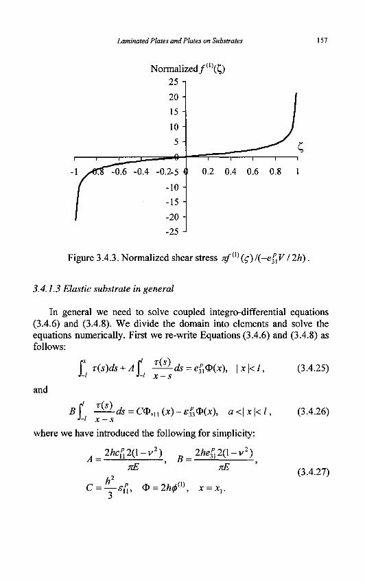
Laminated Plates and Plates on Substrates 157
Normalized/(1)(0 25
20
15
10 H
5 ^
-i 1
-0.6 -0.4 -0.2-5 4 0.2 0.4 0.6 0.8 1
•10
•15
-20 H
-25
Figure 3.4.3. Normalized shear stress ^~('(g)/(-e^V/2h).
3.4.1.3 Elastic substrate in general
In general we need to solve coupled integro-differential equations (3.4.6) and (3.4.8). We divide the domain into elements and solve the equations numerically. First we re-write Equations (3.4.6) and (3.4.8) as follows:
f z(s)ds + A$ - ^ - < & = ef,<B(jt), | J C | < / , (3.4.25) 1-1 i-l x — S
and
B( ^-ds = OJ>,u(x)-ef3(S>ix), a<\x\<l. J-' x - s
where we have introduced the following for simplicity:
. 2hc^2{\-v2) D 2he^2(l-v2) A= , B = —
KE TZE
h1
C = —e{[, <D = 2/^ ( 1 ) , x = xv
(3.4.26)
(3.4.27)
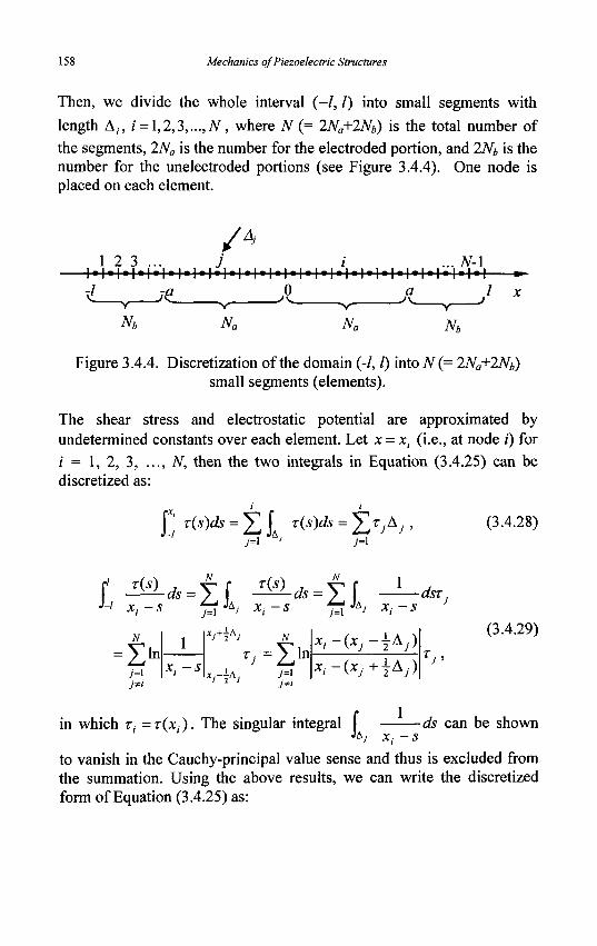
158 Mechanics of Piezoelectric Structures
Then, we divide the whole interval (-/, /) into small segments with length A;, i = 1,2,3,...,N, where N (= 2Na+2Nb) is the total number of the segments, 2Na is the number for the electroded portion, and 2Nb is the number for the unelectroded portions (see Figure 3.4.4). One node is placed on each element.
1 2 3 / '
/ .. T V - 1 , | . | . | . | . | . | . | . | . | . | . | » l ' l » l » l * l » l » l * l » l » l ' l « l » l « l « l
i_ Nb
7<L .0
Na
a I x "V
Nb
Figure 3.4.4. Discretization of the domain (-/, I) into N(= 2Na+2Nb) small segments (elements).
The shear stress and electrostatic potential are approximated by undetermined constants over each element. Let x = xt (i.e., at node i) for / = 1, 2, 3, ..., N, then the two integrals in Equation (3.4.25) can be discretized as:
j j r(s)ds = X jA T^ds = HTJAJ (3.4.28)
J-i x.-s *ri JA, v -,c *ri JA, X,-S J
xt -s
N
= I> 7=1
MJAJ X,-S
X: ~S 7 = I l n t i =
7=1 }*i
7=1 kJ X,S
XI-(XJ-\AJ)
xi-{xJ+\kJ) TJ>
(3.4.29)
f 1 in which r, =T(X ) . The singular integral ds can be shown JA , r — s
to vanish in the Cauchy-principal value sense and thus is excluded from the summation. Using the above results, we can write the discretized form of Equation (3.4.25) as:
Laminated Plates and Plates on Substrates 159
A5>;+^I l n 7=1
i = 1,2,3,..., AT,
7=1 * , - ( * , + 7 A ) -ap 'Si*,*
(3.4.30)
where <D, =0 ( JC , ) and a uniform length for all the elements has been
assumed (i.e., Ay =A , y' = l,2,3,...,Af ). Notice that 0>Nb+l =<&Nb+2
= V, as given in Equation (3.4.7). There are a total of N O Nh+2NC
equations in Equation (3.4.30). Applying the central difference scheme, we have
<-\n(*,) = <->/+!-20,+<-\_i
(3.4.31)
i=2,3,...,Nb,Nb+2Na+\,...,N-\.
Thus, the discretized form of Equation (3.4.26) is found to be
*5> 7=1 7'*'
* < - ( * ; — 2 A )
* , - (* ;+1 A)
i = 2,3,...,Nb,Nb+Na+l,...,N-l,
T V = ^ - ( < D , + 1 - 2 0 , . + < D M ) - ^ 0 , ;
(3.4.32)
in which
0> w*+i (D W*+2AT, = K. (3.4.33)
from condition (3.4.7) or (3.4.9)i should be applied. There are only 2Nb -2 equations in Equation (3.4.32). Two more equations are found by enforcing the zero-slope boundary condition in Equation (3.4.9)2
using the finite difference, that is,
<D, 0>2, Ow_! O, (3.4.34)
There are a total of N + 2Nb equations in Equations (3.4.30), (3.4.32) and (3.4.34), which are used to solve for the N unknowns r, (i = 1,2,3,..., N) and 2Nb unknowns O, , (/* = 1,2,3,..., Nb, Nb+2Na+\,..., N-l, N). Equations (3.4.30), (3.4.32) and (3.4.34) can be written in a matrix form and solved for r and O together or solved for r and <t> separately using partitioning of the whole matrix. For
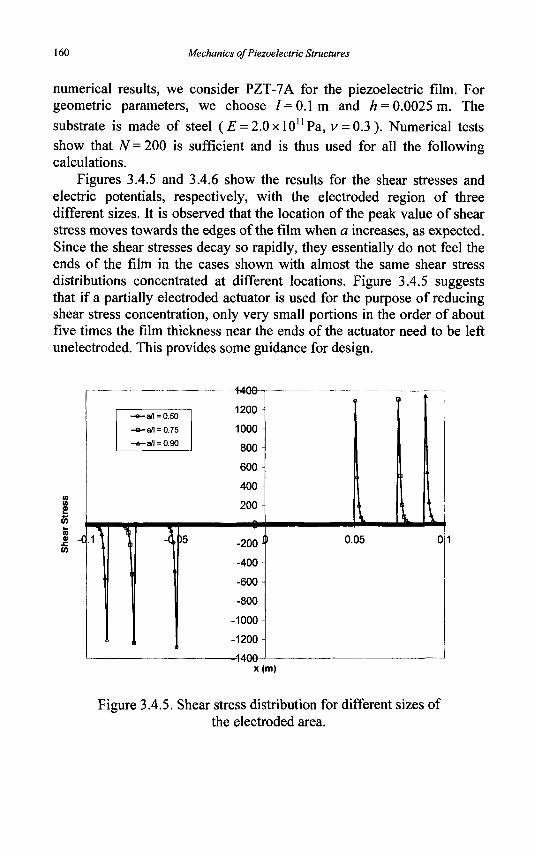
160 Mechanics of Piezoelectric Structures
numerical results, we consider PZT-7A for the piezoelectric film. For geometric parameters, we choose / = 0.1m and h = 0.0025 m. The
substrate is made of steel ( £ = 2.0xl0nPa, v = 0.3). Numerical tests show that N=200 is sufficient and is thus used for all the following calculations.
Figures 3.4.5 and 3.4.6 show the results for the shear stresses and electric potentials, respectively, with the electroded region of three different sizes. It is observed that the location of the peak value of shear stress moves towards the edges of the film when a increases, as expected. Since the shear stresses decay so rapidly, they essentially do not feel the ends of the film in the cases shown with almost the same shear stress distributions concentrated at different locations. Figure 3.4.5 suggests that if a partially electroded actuator is used for the purpose of reducing shear stress concentration, only very small portions in the order of about five times the film thickness near the ends of the actuator need to be left unelectroded. This provides some guidance for design.
-« -a f l = 0.50
-a -a f l = 0.75
- * - a f l = 0.90
.-1400
1200-
1000
800
600
400-
200-
7\ 1
i
)5 .200 *
-400-
-600-
-800
-1000
-1200
1 -4400-J
• i
I 1 \ ) 0.05 0
x(m)
Figure 3.4.5. Shear stress distribution for different sizes of the electroded area.
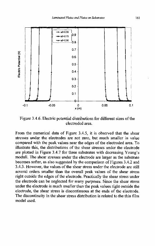
Laminated Plates and Plates on Substrates 161
J
I
1
J
1
-»-a/l=0.50
-e-a/l=0.75
-a-a/l=0.90
0.9
n n -
0.7-
0.6,
0.5-
0.4-
0.3
021 I 0.1 -
I
.
I
I
LL„ -0.1 -0.05 0 0.05 0.1
x(m)
Figure 3.4.6. Electric potential distributiosn for different sizes of the electroded area.
From the numerical data of Figure 3.4.5, it is observed that the shear stresses under the electrodes are not zero, but much smaller in value compared with the peak values near the edges of the electroded area. To illustrate this, the distributions of the shear stresses under the electrode are plotted in Figure 3.4.7 for three substrates with decreasing Young's moduli. The shear stresses under the electrode are larger as the substrate becomes softer, as also suggested by the comparison of Figures 3.4.2 and 3.4.3. However, the values of the shear stress under the electrode are still several orders smaller than the overall peak values of the shear stress right outside the edges of the electrode. Practically the shear stress under the electrode can be neglected for many purposes. Since the shear stress under the electrode is much smaller than the peak values right outside the electrode, the shear stress is discontinuous at the ends of the electrode. The discontinuity in the shear stress distribution is related to the thin film model used.
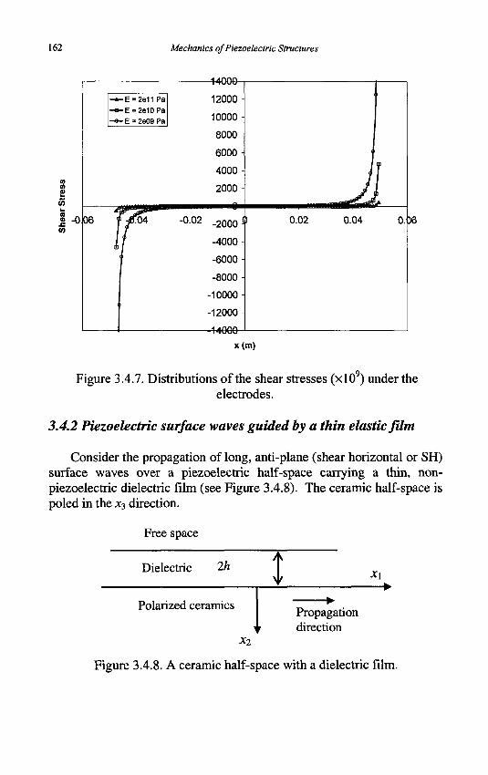
162 Mechanics of Piezoelectric Structures
J *
-E = 2e11Pa -E = 2e10Pa -E = 2e09Pa
06
14000
12000 -
10000
8000
6000
4000
2000
0
-0.02 -2000
-4000 -|
-6000
-8000
-10000
-12000
-14000
0.02 0.04 0.06
x(m)
Figure 3.4.7. Distributions of the shear stresses (xlO ) under the electrodes.
3.4.2 Piezoelectric surface waves guided by a thin elastic film
Consider the propagation of long, anti-plane (shear horizontal or SH) surface waves over a piezoelectric half-space carrying a thin, non-piezoelectric dielectric film (see Figure 3.4.8). The ceramic half-space is poled in the x3 direction.
Free space
Dielectric 2h A
Xi
Polarized ceramics Propagation direction
xi
Figure 3.4.8. A ceramic half-space with a dielectric film.
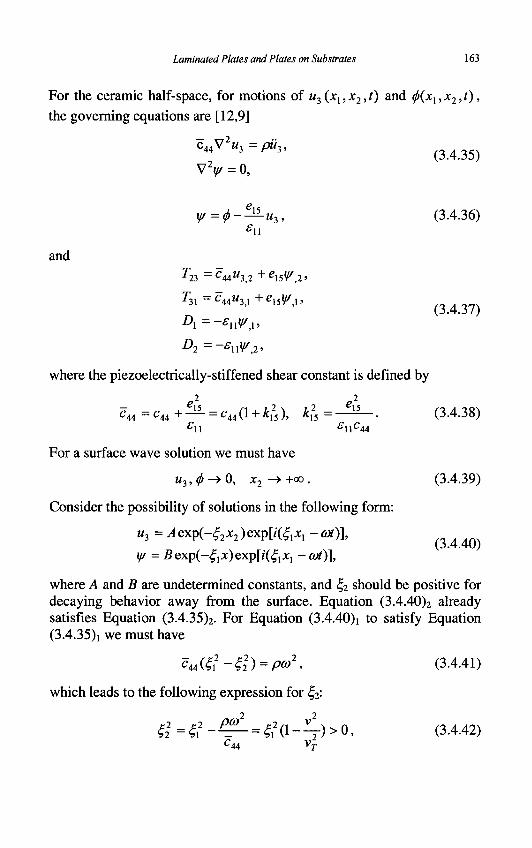
Laminated Plates and Plates on Substrates 163
For the ceramic half-space, for motions of u3(xx,x2,t) and </>{xx,x2,t), the governing equations are [12,9]
(3.4.35)
and
where the
c44V2«3 =pii3,
V:
^23 =
A = D2 =
piezoelectrically-
r> — r* 4
*11
: C44M3,2 +e\5lrY,2'
Cwuxx+ex5yx,
•-suy/a, •stiffened shear constant is
2
defined by
(3.4.36)
(3.4.37)
(3.4.38) SUCA4
For a surface wave solution we must have
w 3 ,^->0, x2-»+oo. (3.4.39)
Consider the possibility of solutions in the following form:
M3 = Aexp(-^2x2)exp[i(^xxx -°)t)]>
y/ = Bexp(-^xx)exp[i(^xxx -at)], (3.4.40)
where A and B are undetermined constants, and £2 should be positive for decaying behavior away from the surface. Equation (3.4.40)2 already satisfies Equation (3.4.35)2. For Equation (3.4.40)i to satisfy Equation (3.4.35)i we must have
cu($-g) = pa>\ (3.4.41)
which leads to the following expression for <fj2:
&=ti - - = £ a - 4 ) > ° - <3-4-42) C44 VT
164 Mechanics of Piezoelectric Structures
where
2 co V = — r
2 C. V r • =
44
P (3.4.43)
The following are needed for prescribing boundary and continuity conditions:
</> = [Bexp(-^x2) + -^-Aexp(-^2x2)]exp[i(^x: -cot)},
(3.4.44) T23 = -[.4c44£2exp(-£2x2)
+ ei5B^ exp{-%xx2)}exp[i{Zxxx -cot)],
D2 = £uB^exp(-^x2)exp[K^xx -cot)].
Electric fields can also exist in the free space of x2 < -2h = 0, which is governed by
V V = 0, x2< 0,
—00. <f> - > 0 , x 2
A surface wave solution to Equation (3.4.45) is
^ = Cexp^jCj )exp[i(£lxl - cot)],
(3.4.45)
(3.4.46)
where C is an undetermined constant. From Equation (3.4.46), in the free space
Di = -^o^iC exp(^x2 )exp[/(^1 j - cot)]. (3.4.47)
The film is assumed to be very thin in the sense that its thickness is much smaller than the wavelength of the waves we are interested in. We use a prime to indicate the elastic and dielectric constants as well as the mass density of the film. Consider a film of a cubic crystal with m3m symmetry. The elastic and dielectric constants are given by
fc'
C12
C12
0
0
0
0
0
0
u12
c 1 2
c'„ 0
0
0
0
0
0
C44
0
0
0
0
0
0
C44
0
0
0
0
c44y
fcn 0
0
0 ^
0 (3.4.48)
Laminated Plates and Plates on Substrates 165
(3.4.49)
For the film, we use the two-dimensional plate equations. This approach was used in [42]. The lowest order effects of the film are governed by the zero-order equations for extension. We have
TZ + T2b (x2 = 0) - T2b (x2 = -2h) = Ip'huf,
D™ + D2 (x2 =0)-D2 (x2 =-2h) = 0, a,b = 1,3.
The constitutive relations for the film are
y(0) _ rP c(0)
DT=4E?\ r,* = lA5,
where
(3.4.50)
cp„ = c'rs ~c'ncZXc'vs, v,w = 2,4,6. (3.4.51)
The fields in the film are
u3=Aexp[i(^xx-o)t)l
0 = Cexp[i(4iX\ - ojt)]. (3.4.52)
Equation (3.4.52) already satisfies the continuity of the mechanical displacement between the film and the ceramic half-space, and the continuity of the electric potential between the film and the free space. From Equation (3.4.50) we obtain:
= Hiefc&A exp[i(£*, - cot)], (3 4 53)
D[0) = 2he'nEl=-2he'njil
= -2he'niJ;xCQxp[i(%xxx -col)].
Substitution of Equations (3.4.44), (3.4.46), (3.4.47) and (3.4.53) into the continuity condition of the electric potential between the ceramic half-space and the film, Equation (3.4.49)i for 6 = 3, and Equation (3.4.49)2
yields
166 Mechanics of Piezoelectric Structures
B + ^-A = C,
-c^A-^-(AcMZ2+el5B^) = -p'<D2A, (3.4.54)
s^C + ^-^B^+s^Q^O, 2«
which is a system of linear, homogeneous equations for A, B and C. For nontrivial solutions the determinant of the coefficient matrix has to vanish
;15
pW-ctef-ML 2«
1
«isft
1
0 2h
£\\h\ £dh\ , r2 + EUhl 2h 2h
= 0. (3.4.55)
which determines the dispersion relation, a relation between co and £i, of the surface wave. In terms of the surface wave speed v = <»/£,, Equation (3.4.55) can be written in the following form:
VVr2
•1 ^ 2 / ^ - l -4+*, 25 c 4 4 \ v\
v15
£u £u
(3.4.56)
where Equation (3.4.42) has been used, and
,.'2 C44 T2 _ _ f l 5
— r » ''is _ -(3.4.57)
When h = 0, i.e., the dielectric film does not exist, Equation (3.4.56) reduces to
jfc4
(l + £u/£0)2
(3.4.58)
Laminated Plates and Plates on Substrates 167
which is the speed of the well-known Bleustein-Gulyaev piezoelectric
surface wave. When k^-Q, i.e., the half-space is nonpiezoelectric,
electromechanical coupling disappears and the wave is pure elastic. In this case, Equation (3.4.56) reduces to
yv'T2 1 ^ 2 / ^ - l - - = 0 , (3.4.59)
'44
which is the equation that determines the speed of Love wave (an anti-plane surface wave in an elastic half-space carrying an elastic layer) in the limit when the film is very thin compared to the wavelength (&A « 1).
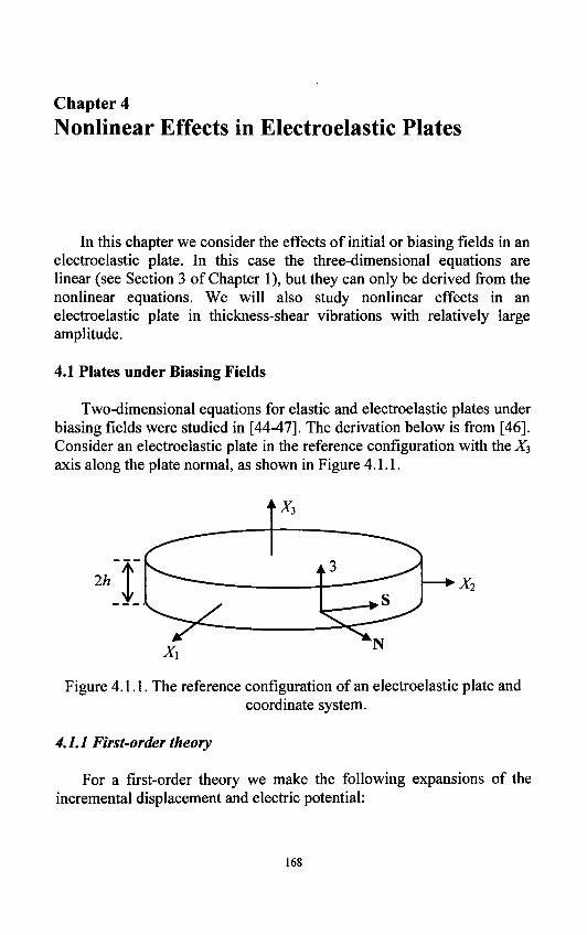
Chapter 4
Nonlinear Effects in Electroelastic Plates
In this chapter we consider the effects of initial or biasing fields in an electroelastic plate. In this case the three-dimensional equations are linear (see Section 3 of Chapter 1), but they can only be derived from the nonlinear equations. We will also study nonlinear effects in an electroelastic plate in thickness-shear vibrations with relatively large amplitude.
4.1 Plates under Biasing Fields
Two-dimensional equations for elastic and electroelastic plates under biasing fields were studied in [44-47]. The derivation below is from [46]. Consider an electroelastic plate in the reference configuration with the X3
axis along the plate normal, as shown in Figure 4.1.1.
X3
2h •X,
Figure 4.1.1. The reference configuration of an electroelastic plate and coordinate system.
4.1.1 First-order theory
For a first-order theory we make the following expansions of the incremental displacement and electric potential:
168
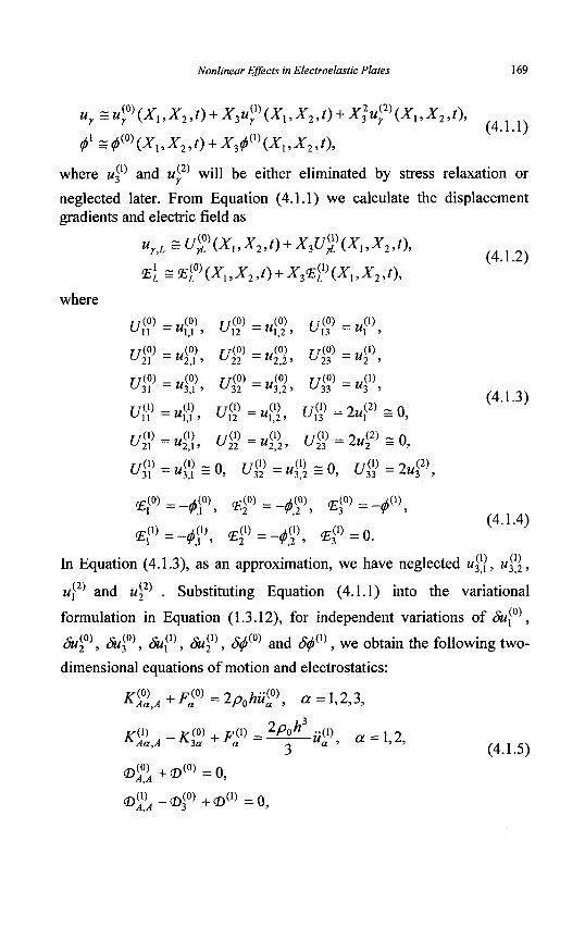
Nonlinear Effects in Electroelastic Plates 169
4>l =<pm(x,,x2 ,o + x3</>m(X,,x2,t),
where wf and w£2) will be either eliminated by stress relaxation or
neglected later. From Equation (4.1.1) we calculate the displacement gradients and electric field as
(4.1.2)
where f/(0) _ M(0) f / (0) _ (0) f / (0) (1) ^11 ~ u\,\ ' ^12 — wl,2 ' ^13 Ml 3
21 — 2 1 ' 22 — 2 2' 23 — 2 '
f/(0) _ M(0) f /(0) _ (0) f / (0) _ (1) u 3 1 — "3 ,1 » ^ 3 2 — "3,2' u 3 3 — " 3 '
21 — 2 1 ' 22 — 2 2 ' 23 — £t4y = U j
£/Jl>=i/g=o, ^ = „ ( ; ) = o , t/3(?=2«|2),
E . ^ - ^ , £f=-^(2
0), <E^=-^l\
(4.1.3)
(4.1.4) ',i >
In Equation (4.1.3), as an approximation, we have neglected u^\, u3\,
u\2) and w22) • Substituting Equation (4.1.1) into the variational
formulation in Equation (1.3.12), for independent variations of Su\°\
Su<£\ Suf\ Su\l\ Su2\ S<f>{0) and # ( 1 ) , w e obtain the following two-
dimensional equations of motion and electrostatics:
&^-K%+FV = *ȣ-u*\ a = 1,2, ( 4 L 5 )
©W + © (0)=0,
< ^ - < } + c D ( 1 ) = 0 ,
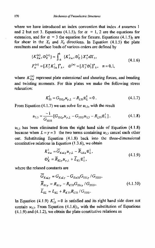
170 Mechanics of Piezoelectric Structures
where we have introduced an index convention that index A assumes 1 and 2 but not 3. Equations (4.1.5)i for a = 1, 2 are the equations for extension, and for a = 3 the equation for flexure. Equations (4.1.5)2 are for shear in the X\ and X2 directions. In Equation (4.1.5) the plate resultants and surface loads of various orders are defined by
{*£>,©£>} = f {K'Ka,cDlK}X"3dX3,
J~h (4.1.6) F^=[X"3Kla]
h_h, <DW =[X;<D\£h, 11 = 0,1,
where K^l represent plate extensional and shearing forces, and bending and twisting moments . For thin plates we make the following stress relaxation:
K\,=G„LrurL-RLilT}L=Q. (4.1.7)
From Equation (4.1.7) we can solve for W33, with the result
"3,3 = — \G^LruyL -G3333M33 -RL33ElL]. ( 4 . 1 . 8 )
^3333
M33 has been eliminated from the right hand side of Equation (4.1.8) because when L -y = 3 the two terms containing W33 cancel each other out. Substituting Equation (4.1.8) back into the three-dimensional constitutive relations in Equation (1.3.6), we obtain
(4.1.9)
where the relaxed constants are
^KccLy ~ ^KccLy ~ &Kaii^i^Ly ' ^3333»
RKLy = RKLy ~ RK33G33Lr /G3333, (4.1.10)
LftL — LKL + ^AT33^L33 ' ^3333-
In Equation (4.1.9) £33 = 0 is satisfied and its right hand side does not contain 1/3,3. From Equation (4.1.6)1, with the substitution of Equations (4.1.9) and (4.1.2), we obtain the plate constitutive relations as
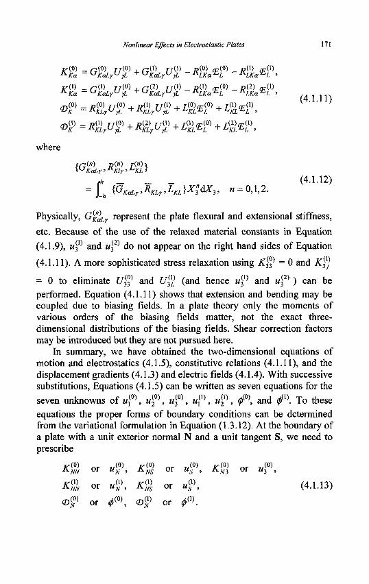
Nonlinear Effects in Electroelastic Plates 171
K(S>) _ a(f>) i-r(O) , W l ) TJ(\) _ R(0) ^ ( 0 ) _ n(l) - (1) A K a -KjKaLyUyL + {JKaLyUyL ^LKa^L ^LKa^L >
K(Xi - Gm 7/(0) , GP) TTW _ D ( D «r(0) _ D ( 2 ) C ( 1 ) ^Ka ~ UKaLyUyL + UKaLyUfi ^LKa^L ^LKa^L »
(4.1.11)
^KLywyL T ^ K L y ^ y L
where
{G&r,*g,Z<5>> ,* _ _ _ „ (4.1.12)
= lh {GKaLr,RKLy,LKL}X3"dX3, n = 0,1,2.
Physically, G j ^ represent the plate flexural and extensional stiffness,
etc. Because of the use of the relaxed material constants in Equation
(4.1.9), u® and u^ do not appear on the right hand sides of Equation
(4.1.11). A more sophisticated stress relaxation using K^* = 0 and Ky
= 0 to eliminate U$ and U^l (and hence u^ and w|2) ) can be performed. Equation (4.1.11) shows that extension and bending may be coupled due to biasing fields. In a plate theory only the moments of various orders of the biasing fields matter, not the exact three-dimensional distributions of the biasing fields. Shear correction factors may be introduced but they are not pursued here.
In summary, we have obtained the two-dimensional equations of motion and electrostatics (4.1.5), constitutive relations (4.1.11), and the displacement gradients (4.1.3) and electric fields (4.1.4). With successive substitutions, Equations (4.1.5) can be written as seven equations for the
seven unknowns of w,(0), uf^, uf*, Wj(1), u^, <f\ and 0(1). To these equations the proper forms of boundary conditions can be determined from the variational formulation in Equation (1.3.12). At the boundary of a plate with a unit exterior normal N and a unit tangent S, we need to prescribe
(4.1.13) A-NN
(D ( 0 )
or
or
or
K ( 0 ) UN >
«$>,
#<»>,
Km
(Dm
or
or
or
M ( 0 )
w(1)
"S '
<?>m.
K(0) or w(0)
" 3 »
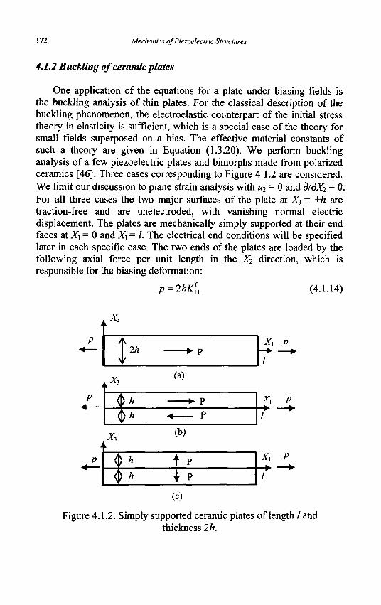
172 Mechanics of Piezoelectric Structures
4.1.2 Buckling of ceramic plates
One application of the equations for a plate under biasing fields is the buckling analysis of thin plates. For the classical description of the buckling phenomenon, the electroelastic counterpart of the initial stress theory in elasticity is sufficient, which is a special case of the theory for small fields superposed on a bias. The effective material constants of such a theory are given in Equation (1.3.20). We perform buckling analysis of a few piezoelectric plates and bimorphs made from polarized ceramics [46]. Three cases corresponding to Figure 4.1.2 are considered. We limit our discussion to plane strain analysis with u2 = 0 and d/dX2 = 0. For all three cases the two major surfaces of the plate at X3 = ±h are traction-free and are unelectroded, with vanishing normal electric displacement. The plates are mechanically simply supported at their end faces at X\ = 0 and X\ = I. The electrical end conditions will be specified later in each specific case. The two ends of the plates are loaded by the following axial force per unit length in the X2 direction, which is responsible for the biasing deformation:
p = 2hK°n. (4.1.14)
\ x i
1
> 2h
/ * P
x, (b)
Xi P
.X
$ h
tyh
(a)
A P
v /
X, P
Q h ^ h
t P I P
X, P
(c)
Figure 4.1.2. Simply supported ceramic plates of length / and thickness 2h.
Nonlinear Effects in Electroelastic Plates 173
(4.1.15)
4.1.2.1 A single-layered plate
Consider a ceramic plate poled in the X\ direction as shown in Figure 4.1.2(a). The material matrices are in Equation (2.3.45). The plate is electroded at its two end faces at X\ = 0 and X\ = I. The electrodes are shown by thick lines in the figure. When the initial load p is being applied, the end electrodes are shorted to eliminate the initial electric field E\ which otherwise would exist. Once p is already loaded, there exist initial charges on the end electrodes. The electrodes are then opened during the incremental flexural deformation and there are no incremental charges on these electrodes. Therefore for the incremental fields the electric displacement vanishes at both ends. The governing equations for the incremental fields take the form
G(0) w(0) + G(0) um +R(0)d>m = 0 "1313M3,11 + L r1331M l , l + A 3 1 3 r , l ~ u>
Offi -*«> -4W -#Wt+4^(1) -o, and the boundary conditions are
«<°>=0, X ,=0 , / ,
Ki?=G{?uuU+R^=0, Xx=0,l,
<D[0) = -Ihe^f = 0, Xx = 0, /,
0 1 « = O « - ^ V J > = 0 , Xl=0,l, where
C = 2 ^ 4 4 + p, GZ = G<?>3 = G3(?>, = 2te44,
G'ft = i h2 (2hcx + p), tf <°> = 4°> = 2te15,
RV>-lh3e rm--h3? rm-2hr (4.1.17) - " i l l _ ~ " e 3 3 ' M l - ~ - " f c 3 3 > ^ 3 3 - z " £ l l >
2 2 — _ M3 — _ ^31^31 — _ ^31 C33 _ C33 ' e 3 3 ~ e 3 3 ' £33 ~ ff33 H •
C l l C l l C l l
(4.1.16)
174 Mechanics of Piezoelectric Structures
In Equation (4.1.16)2 the bending moment K$ is coupled to
(E,(1) = -<j>^ through e33 as expected. Furthermore, for the transverse
shear force we have K$? = G^\3u^ + G^u^ + R^m which is L13
coupled to £30) =-<j)(-X) through e\5 as expected. Equations (4.1.15)3 and
(4.1.16)3 show that 0(o) is a constant which can be taken to be zero. Let
i40) = A sin £T,, Wl(1) = B cos £Y,,
^ ( 1 ) =Ccos^r„ (4.1.18)
where A, B, and C are undetermined constants and <f = id I. The boundary conditions in Equation (4.1.16) are satisfied automatically. Then the buckling load can be determined from the following equations obtained by substituting Equation (4.1.18) into Equation (4.1.15)1,2,4:
:2n(0) ;(0) ( ° ) r - 1
^ 3 % ^ + C ^ i +G3<8I)2> + tf2J?ffi +4°1)C = 0, (4.1.19)
For non-trivial solutions of 4, 5, or C, the following condition must be satisfied
<?2G(0)
h "1313
£ ^ 3
^
#7(0) S"l331
<52G(2) + G ( 0 )
S "1111 + <J3131 <52/?(2) + /? ( 0 )
£ -"ill + ^ 3 3 1
&&
*2*ffi+*Si - ( ^ + ^ )
= 0,
which can be written as
ampm2+bmpm+cm=0,
where
(4.1.20)
(4.1.21)
PiX) = 2hc
X0 - n 33
h a - A Q ,
".(» A0+-' 33
(A0+l)c44 + V l 2 5 + ( V 3 3 + e 1 5 )
£•[, +/ t0£'33
.0) - .
' 3 3 / l 0
c 44 + A i ^ i s "r AnC-i i C-i-iC , 0 c 3 3 c 3 3 i - 4 4
fu + / l 0 £ ,3 3
(4.1.22)
Nonlinear Effects in Electroelastic Plates 175
Since Xo « 1 for a thin plate, it follows from Equation (4.1.22) that (bm)2 »4amcm and bm»am for thin plates. Hence, an approximate solution to Equation (4.1.21) can be found as
p bm
f amcv)\ 1 + -
(* ( 1 ) ) 2 y (4.1.23)
Our main interest is the effect of piezoelectric coupling on the buckling load. To see this more clearly, we let c44 —> °° in Equation (4.1.23), which effectively eliminates plate shear deformations and the related piezoelectric coupling through e15. We then expand Equation (4.1.23) into a polynomial of Xo that is small. This leads to
pm*-A0(l + A0P), P=ei3/Qc33eu), (4.1.24)
where k2 may be considered as an electromechanical coupling factor.
Under our notation -Ao is the dimensionless buckling load from an elastic analysis without considering the piezoelectric effect. The second term on the right hand side of Equation (4.1.24)i represents the effect of piezoelectric coupling due to e33. This additional term is proportional to
k2, which ranges from 0.1 to 0.6 for most polarized ceramics. Since
A:2 is multiplied by Ao, which is a small number, the piezoelectric
modification on the buckling load is a small addition to the elastic buckling load. Hence an elastic analysis without considering the piezoelectric effect gives a conservative estimate of the buckling load.
4.1.2.2 A bimorph with in-plane poling
In this case we consider a ceramic bimorph as shown in Figure 4.1.2(b). The end faces are unelectroded. The governing equations for the incremental fields are
G(0) M(0) + Gm
M(1) - 0 "1313 "3,11 + ( J 1 3 3 1 " 1 , 1 _ u>
Gf&nff, + B&OS ~G3%«S> - G<?3><» =0,
4WiV-4°3V(,) = o,
176 Mechanics of Piezoelectric Structures
with the following boundary conditions:
,(°) :(2) „(D (DwlW - i ^=c?, iMy+^wr=o, *i=<w
<D (0)
w y - w j = ° . i=o,/, (4.1.26)
where the plate material constants are as in Equation (4.1.17) plus
Rm = h2e 33- (4.1.27)
In Equation (4.1.26)2 the bending moment K$ is coupled to
<£• (°) - _ M « » ^ I J through e33 as expected. We note that Equations (4.1.25)4
and (4.1.26)4 imply 0(1) = 0. Let
uf]=A sin £Yi, Ml(1) = 5 cos £r,,
/ ^ - D C O S ^ , (4.1.28)
which satisfy the boundary conditions in Equation (4.1.26) when £ = nil. Eliminating 0(O) from Equation (4.1.25)2 and Equation (4.1.25)3, and substituting Equations (4.1.28)i>2 into the resulting equation and Equation (4.1.25)i, we obtain
£2G{3V + ^ ( 3 V = 0,
&£U + {? [Gffl, + (Iff )-' tfffi2 ] + G% }B = 0.
For nontrivial solutions of y4 and 5, the following must be true:
(4.1.29)
G(o) "1331
or
£ G(0)
h "1313
S"3113 S L " l l l l + < A l J -"ill J + "3131
fl(2)^(2)2+fe(2)-(2)+c(2)=()
= 0. (4.1.30)
(4.1.31)
Nonlinear Effects in Electroelastic Plates 111
where
P(2)
",(2) -
2hc a (2) _
H)' 33
ftW=yL+ — '0 ^ -C33
3 _ 2 __j ( / l 0+l)c 4 4+-/ l 0e
33 f33 (4.1.32)
,(2)
'33
1 It ' — 2 1 •-0M4 L0 t-44o33c33°33
An approximate solution to Equation (4.1.31) is given by
„(2) (
? P ) -6<2>
1 + (6 (2 ))2
(4.1.33)
Letting C44 -^ «> in Equation (4.1.33) and expanding the resulting expression into a polynomial of Xo, we have
-M) 3 n * - ^ 0 0 + T * 3 3 )> ^33 = g33 / ( C 3 3 f 33 ) • (4.1.34)
Comparing Equation (4.1.34)! with Equation (4.1.24)l5 we notice the important difference that in Equation (4.1.34)i the piezoelectric modification on the buckling load is not multiplied by the small number Ao. This is because in Equation (4.1.15) the plate piezoelectric coefficient
(i) is R^i is proportional to h . However, in Equation (4.1.25) R\
proportional to h2 and it is the squares of the piezoelectric coefficients that appear in the buckling loads. Therefore the piezoelectric effect on the buckling load is much stronger in Case (b) than in Case (a).
4.1.2.3 A bimorph with thickness poling
The third case is a ceramic bimorph as shown in Figure 4.1.2(c). The plate is electroded at X\ = 0 and X\ = I, with shorted and grounded electrodes. The governing equations take the following form:
178 Mechanics of Piezoelectric Structures
G(0) w(0) + G(0) w(1) + Rm</>(1) - 0 Lr1313M3,ll +*J1331Ml,l +Km<P,U _ U >
C M , -G3(?uy -««,w+[*,<& - * » = ° >
The boundary conditions are
M(°>=0, X , = 0 , / ,
^n )=G1(1
2i ),«S )+A2e3^ (1)=0> X , = 0 , / ,
0<°>=O, X , = 0 , / ,
^ > = 0 , X , = 0 , / ,
(4.1.35)
(4.1.36)
G ( 2 ) ^1111
G(0)
^1331
DO) •"311
cii =
*33 =
= U2(2hcn +
_ ^ 3 1 1 3 _ ^3131
- fc2e Z(0) -" K 3 1 ' ^11
C l l _ C 1 3 ' C33>
£ 3 3 + e 3 2 3 / c 3 3 -
P), G®3
i = 2/zc44,
= 2fc44 + p,
D(D •"113
2/ , r . r(2) _
e31 = e31 -e33<
=
2 3
' 31
A 131
/ ? 3 f f u ,
/c33»
A2.15
J-(O) -^33 2hs33, (4.1.37)
In Equation (4.1.36)2 the bending moment K^ is coupled to
(E3(0) = -<j>m through e31 as expected. In this case 0(o) is zero. We let
ui0) = A sin EC., w,(1) = B cos £r, , (4.1.38)
<f>m=C sin D{u
which satisfy the boundary conditions in Equation (4.1.36). Substituting Equation (4.1.38) into Equations (4.1.35)^2,4:
^ G ^ + V + ffiC^O, tGV\3A + (Z2Gtfu + G3%)£ + £(*1
(30i - < ) C = 0, (4.1.39)
?B®A + £(*g> - < ) * - (£2Z<2> + l£> )C = 0.
Nonlinear Effects in Electroelastic Plates 179
For nontrivial solutions of A, B, or C, the following condition must be satisfied:
£ 2 G ( 0 ) ^ ( 0 )
1313 V-M331 (0) e 2 ^ ( 2 ) , r(0)
or
where
« 3
^3% ^Gfft+G3% - W ? , - ^ , )
^ 3 -^3 (1 )1-^ )
1) - ( ^ ^ + 4 ) )
a ( 3 y 3 ) 2 + i ( 3 ) - ( 3 ) + c ( 3 ) = ( ) ;
= 0, (4.1.40)
(4.1.41)
2hcn
,(3) : ^0>
(A0 + l)c44 + 3A0[A0el5+(el5-e3l) ]
,(3) A0c44 +
4 ( V n + ff33>
4(Vl l+^33)
(4.1.42)
An approximate solution to Equation (4.1.41) is found to be
p ( 3 ) « ° (3)
6(3)
^ fl(3)c(3)^ 1 +
(* ( 3 ) )2 (4.1.43)
Letting c44—» °° in Equation (4.1.43) and expanding it into a polynomial of Ao, we obtain
3 — — p0) * - A 0 (1 + - # , ) , ^ - g3
2 /(Cnff33 ) (4.1.44)
which shows the same behavior as Equation (4.1.34). Buckling analysis of circular piezoelectric plates using two-dimensional equations was performed in [47].
4.2 Large Thickness-Shear Deformations
We are interested in thickness-shear vibrations with relatively large shear deformations [48] for a plate whose reference configuration is
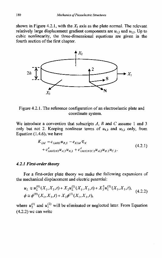
180 Mechanics of Piezoelectric Structures
shown in Figure 4.2.1, with the X-i axis as the plate normal. The relevant relatively large displacement gradient components are Mi;2 and w3>2. Up to cubic nonlinearity, the three-dimensional equations are given in the fourth section of the first chapter.
2h
X2
X1
Figure 4.2.1. The reference configuration of an electroelastic plate and coordinate system.
We introduce a convention that subscripts A, B and C assume 1 and 3 only but not 2. Keeping nonlinear terms of w^ and M3>2 only, from Equation (1.4.6)i we have
K-UA —CLMRS"R,S Up C 6 KLM^K
+ CLMA2B2UA,2UB,2 + CLMA2B2C2UA,2UB,2UC,2 •
(4.2.1)
4.2.1 First-order theory
For a first-order plate theory we make the following expansions of the mechanical displacement and electric potential:
uL = M f (X, ,X3,t) + X2uf (Xx ,X3,t) + Xlu™ (X,, X 3 , 0 ,
~ A°) </> = <l)w{Xx,X„t) + X2<l>w{Xx,X„t), 0)/ (4.2.2)
where u^ and «[2) will be eliminated or neglected later. From Equation (4.2.2) we can write
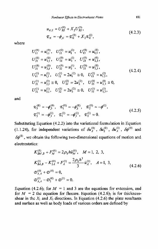
Nonlinear Effects in Electroelastic Plates 181
UR,S ~ URS + XlURS
^=-^=40 )+^41 ) (4.2.3)
where K '
iy(0) _ ,.(0) r7(0) _ (l) f /(0) _ (0) ^11 — " 1 , 1 > ^ 1 2 — "1 ' UU ~ "1,3 '
|-/(0) _ M(0) r /(0) _ (1) rr(0) _ (0) U21 — "2,1 ' u 2 2 — "2 ' u23 ~ "2,3 >
TT(0) _ M(0) r /(0) _ (1) r /(0) _ (0) u 31 — " 3 , 1 > * ^ 3 2 — "3 ' ^ 3 3 ~ "3,3 >
£ / « = « « , tfg> = ^ = 0, ^ = « g ,
£ / « = « g = 0 , ^ = 2 M < 2 ) , ^ = ^ = 0 ,
[ / « = < > , I/£>=2«<»=0, C /«=«« ,
(4.2.4)
and
-E3(1)=-^31), «E1
(1)=-^(1
1), fE«=0. (4.2.5)
Substituting Equation (4.2.2) into the variational formulation in Equation
(1.1.24), for independent variations of Su(°}, Suf\ Suf , 8<t>{0) and
S<f>m, we obtain the following two-dimensional equations of motion and
electrostatics:
'(0) . n.(0) _ryn , . . ( 0 )
KBlB-K?j+FV=lef.ii<}\ A = l,3,
<^+© ( 0 ) =0 ,
© ^ - © f + © ( , ) = 0 .
(4.2.6)
Equation (4.2.6)i for M = l and 3 are the equations for extension, and for M = 2 the equation for flexure. Equation (4.2.6)2 is for thickness-shear in the X\ and XT, directions. In Equation (4.2.6) the plate resultants and surface as well as body loads of various orders are defined by
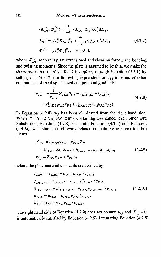
182 Mechanics of Piezoelectric Structures
{K<>>,<DP}=lh {Km,cDK)Xn2dX2,
F™ = [X"2K2M]h_h + \[h PJMXn2dX2, (4.2.7)
<DW =[X"2cD2f_h, n = 0, 1,
where K^ represent plate extensional and shearing forces, and bending and twisting moments. Since the plate is assumed to be thin, we make the stress relaxation of K22 = 0. This implies, through Equation (4.2.1) by
setting L = M = 2, the following expression for w2,2 in terms of other components of the displacement and potential gradients:
U22 = \C22RSUR,S ~C2222M2,2 ~eK22^K
c-mi (4.2.8) + C22A2B2UA,2UB,2 + C22A2B2C2UA,2UB,2UC,2>-
In Equation (4.2.8) «2,2 has been eliminated from the right hand side. When R-S = 2 the two terms containing 1/2,2 cancel each other out. Substituting Equation (4.2.8) back into Equation (4.2.1) and Equation (1.4.6)2, we obtain the following relaxed constitutive relations for thin plates:
K-LM ~CLMRSUR,S ~eKLM^K
+ CLMA2B2UA,2UB,2 + CLMA2B2C2UA,2UB,2UC,2 ' (4.2.9)
^K =eKRSUR,S +£KL<EL>
where the plate material constants are defined by
CIMRS ~ CLMRS ~CLM22C22RS ' C2222 ' — e e I CLMA2B2 ~CLMA2B2 ~ CLM22C22A2B2 ' C2222 '
CLMA2B2C2 ~ CLMA2B2C2 ~ CLM22C22A2B2C2 ' C2222 ' (4.2.10)
eKLM ~eKLM ~ CLM22eK22 ' C2222 '
£KL = EKL +eK22eL22 'C2222.-
The right hand side of Equation (4.2.9) does not contain w2,2 and K22 = 0 is automatically satisfied by Equation (4.2.9). Integrating Equation (4.2.9)
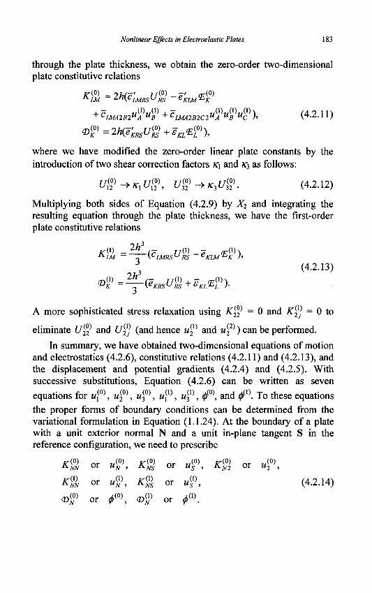
Nonlinear Effects in Electroelastic Plates 183
through the plate thickness, we obtain the zero-order two-dimensional plate constitutive relations
K(0) -2h(c' U(0) -e' <F(0)
^C1MA2B2UA UB + LIMA2B2C2UA UB "C h \?+.A.ll)
< =2h(e'KRSU$ + SKL<ET),
where we have modified the zero-order linear plate constants by the introduction of two shear correction factors K\ and KT3 as follows:
E/g>->*,£/£>, Ug-ncM*- (4-2-12)
Multiplying both sides of Equation (4.2.9) by X2 and integrating the resulting equation through the plate thickness, we have the first-order plate constitutive relations
a ) _M_(- ? / ( l ) _ - ~(1K
(4.2.13)
A more sophisticated stress relaxation using K$ = 0 and K$ = 0 to
eliminate Uf^ and Uy (and hence u^ and u^) can be performed.
In summary, we have obtained two-dimensional equations of motion and electrostatics (4.2.6), constitutive relations (4.2.11) and (4.2.13), and the displacement and potential gradients (4.2.4) and (4.2.5). With successive substitutions, Equation (4.2.6) can be written as seven
equations for w}0), w£0), uf^, u^, uf*, (ff0\ and 0(1). To these equations the proper forms of boundary conditions can be determined from the variational formulation in Equation (1.1.24). At the boundary of a plate with a unit exterior normal N and a unit in-plane tangent S in the reference configuration, we need to prescribe
(4.2.14)
K(0)
Km
<D ( 0 )
or
or
or
M ( 0 ) UN >
um
"N > ^ ) ,
A: ( 0 )
Km
<D (1 )
UN
or
or
or
M ( 0 ) US '
w ( 1 )
"S '
^ ( 1 ) .
KN2 or 4
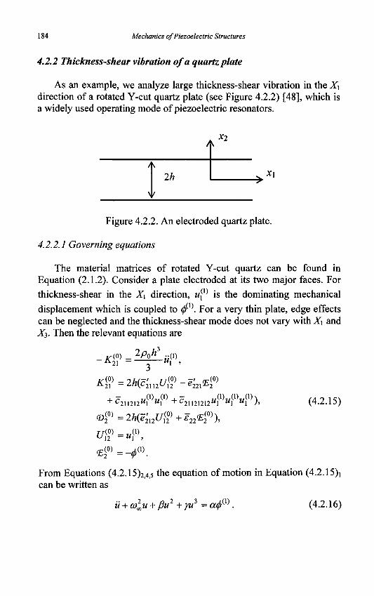
184 Mechanics of Piezoelectric Structures
4.2.2 Thickness-shear vibration of a quartz plate
As an example, we analyze large thickness-shear vibration in the Xi direction of a rotated Y-cut quartz plate (see Figure 4.2.2) [48], which is a widely used operating mode of piezoelectric resonators.
2h
X2
X\
Figure 4.2.2. An electroded quartz plate.
4.2.2.1 Governing equations
The material matrices of rotated Y-cut quartz can be found in Equation (2.1.2). Consider a plate electroded at its two major faces. For
thickness-shear in the X\ direction, M](1) is the dominating mechanical
displacement which is coupled to 0(1). For a very thin plate, edge effects can be neglected and the thickness-shear mode does not vary with X\ and X3. Then the relevant equations are
.3
• A : ( 0 )
-^-21
Ipjt ;0)
K{0) -2h(c' f/(0) -e' <E(' JS.2\ — ''K.L2U2U12 ^221-^2
(0)
+ C
,(0)
uiV+c 211212"! " 1 21121212"! 0)„0)„(Dl
w; 'u\'u i "i (4.2.15)
U<»=«?\ <E
From Equations (4.2.15)2,4,s the equation of motion in Equation (4.2.15)! can be written as
U + a>^u + j3u +yu -a</> 3 - „JSX) (4.2.16)
Nonlinear Effects in Electroelastic Plates 185
In Equation (4.2.16) we have denoted
u=u\x\ ml = 3c2ll2/(p0h2), a = -3e22i/(p0h
2),
K"l c2112' g221 ~ ""ie221'
2_K2 U26 j-2 _ (4.2.17)
12 jt en{c66+eule21)
P = 3c2U2l2/(p0h2), 7 = 3c2U2]2l2/(p0h
2),
where the thickness-shear correction factor is taken from [27]. In Equation (4.2.17), co is the fundamental thickness-shear frequency from a linear solution. We want to study free and forced vibrations near 0) .
4.2.2.2 Free vibration
For free vibrations we look for a periodic solution with undetermined frequency at and amplitude A to the homogeneous form of Equation (4.2.16). For rotated Y-cut quartz, ft = 0 and therefore the quadratic nonlinear term in Equation (4.2.16) disappears. Substituting u = Acoscot into Equation (4.2.16) (with V = 0), and neglecting the cos3c* term, we obtain
-co2A + colA+-YA3 = 0 . (4.2.18) 4
Equation (4.2.18) yields the following expression for the nonlinear resonant frequency
co=la)l+?-rA2 =ft,M(l + f - ) , (4.2.19) V 4 &ol
and the following corresponding free vibration mode
u = A c o s K ( 1 + - ^ - ) f ] . (4.2.20)
Equation (4.2.19) shows that for large amplitude vibrations the frequency becomes amplitude dependent.
4.2.2.3 Forced vibration
Next consider electrically forced vibrations under a voltage across the thickness of the plate with <p(±h) = ±0.5Fcoso*. Then Equation
186 Mechanics of Piezoelectric Structures
(4.2.2)2 implies that
0 ^ = 0 , ^ = — c o s a * . 1h
(4.2.21)
*(D With f-' from Equation (4.2.21), Equation (4.2.16) can be written as
.. 2 3 aV u + coxu + cu + yu = cos cot,
2h
(4.2.22)
where we have also introduced a damping term with a damping coefficient c = 2(Ut0£= afe/g. C is the relative damping coefficient and Q is the quality factor. We look for a solution to Equation (4.2.22) in the following form:
u = A cos(cot + y/), (4.2.23)
where A and (//are undetermined constants. Substituting Equation (4.2.23) into Equation (4.2.22), neglecting the cos3(cot+w) term, and collecting the coefficients of sine* and cosa#, we obtain
[{col, -co2)A + — yA3]cosy/-cAcosini// = , 4 2/z
[(col -co1)A + — yA^^smy/ + cAcocosiff = 0.
(4.2.24)
Multiplying Equations (4.2.24)12 by cosy/and sin wrespectively and then adding them, and multiplying (4.2.24)i2 by sin y/and cosy/respectively and then subtracting one from the other, we have
aV -cosy,
(4.2.25) (al-co2)A + \yA'
2h
aV . cAco = suw.
2h Y
Squaring both sides of Equation (4.2.25)i>2 and then adding them yields
(4.2.26) 2 „ 2 N J , ^ ,3,2 . ,„Ar*Jl _ (aV \l [(col -a>l)A + -yA*Y + (cAa>Y = (—) 4 2/z
We are interested in resonant behaviors near co<o. Therefore we denote
co-cox + Aco. Then col -co2 = -2coxA.co, and Equation (4.2.26) can be
written as
Nonlinear Effects in Electroelastic Plates 187
(Aft)-lyA1
-)2+^r=( 80^ 4
from which we can solve for Aft) :
av
aV )2
Aft) = ±— [(-8« 2lv2A&> ,4
) -c ] 2 l 2
(4.2.27)
(4.2.28)
We calculate the electric current flowing in or out of the driving electrodes, which is important to resonator design. From Equations (4.2.15)3, (4.2.17) i, and (4.2.23) we have, for the free electric charge per unit undeformed area of the electrode at X2 = h
Qe = D<0)
= -(KT1e2 6w-e2 20u) (4.2.29) 2h
- ~Ki^26u ~ -^ie26Acos(ox + y/),
where, for near resonance behavior, we have neglected the electrostatic term in the expression of Qe which is much smaller than the piezoelectric term. Then the current flows out of the electrode is
Qe =-Kle26A(osm(ox + y/) = I sin(ox + y/),
-Kxe26AC0 = -•Kxe26A(Q„ (4.2.30)
From Equations (4.2.30)2 and (4.2.28), we obtain the frequency-current amplitude relation
Aa> = 3y
8ft). + 1
2hl
— \ 2
— C
1/2
(4.2.31)
Quartz is a material with very little damping. We choose the quality factor to be Q = 105. Consider a 1 MHz fundamental mode resonator with h = 0.8273 mm. The frequency-current amplitude relation predicted by Equation (4.2.31) is plotted in Figure 4.2.3, which is typical for nonlinear resonance.
The vertices of the curves in Figure 4.2.3 fall on a parabola as predicted by an approximate analysis from the three-dimensional equations [49]. The Equation for the corresponding parabola predicted by the two-dimensional equations here is Equation (4.2.31), without the last term en the right hand side. In Figure 4.2.4 we plot the two parabolas from the two- and three-dimensional solutions as a comparison. It can be seen that the two parabolas are very close to each other.
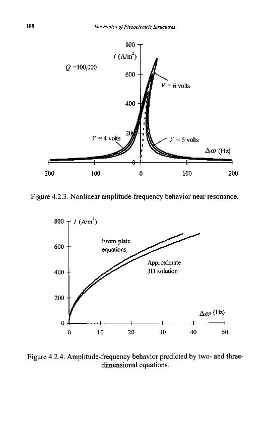
188 Mechanics of Piezoelectric Structures
Q =100,000
800-r
/ (A/m2)
600--
400
V = 6 volts
V = 4 volts 20d
F = 5 volts Aft> (Hz)
-200 -100 100 200
Figure 4.2.3. Nonlinear amplitude-frequency behavior near resonance.
800 T / (A/m )
600 --
400 --
200 --
10 20 30 40 50
Figure 4.2.4. Amplitude-frequency behavior predicted by two- and three-dimensional equations.
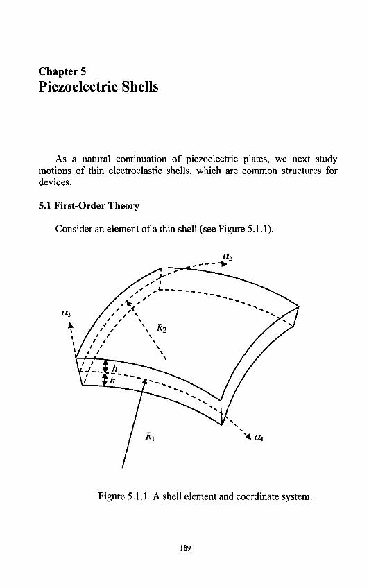
Chapter 5
Piezoelectric Shells
As a natural continuation of piezoelectric plates, we next study motions of thin electroelastic shells, which are common structures for devices.
5.1 First-Order Theory
Consider an element of a thin shell (see Figure 5.1.1).
Figure 5.1.1. A shell element and coordinate system.
189
190 Mechanics of Piezoelectric Structures
(X\ and a2 are the middle surface principal coordinates, and a3 is the thickness coordinate. (a^o^Cfe) is an orthogonal curvilinear coordinate system. The thickness of the shell, 2/z, is much smaller than the radii of curvature R\ and R2 of the middle surface. Let Ax and A2 be the Lame coefficients corresponding to ot,\ and a2 at the middle surface. The metric in {a\,a2,(Xj) is given by Ai(l-a3/R{), A2{\-a3IR2), and 1, which determines the tensor operations in (a\,a2,a3). The strain-displacement relations take the following form [50]:
Su=-1
«, 4(1 + ^ )
du}
da, l- +
R
S22 - • 1
a, M1 + -?)
du-
da1
2 +
«2 94 , Afo 1
y42 9«2 Rx
u, 8A2 A2u3 1
A[ da, R2
5
0 _ 8U3 ' 3 3 - a
oa3
(5.1.1)
a, 2S23=^2(1 + — ) ~ R-, da-,
2S3l = 4 ( 1 + - ) : a
a,
i?, 5a3 40 + )
+ <9w,
4 ( 1 + ^ - ) ^ ' &
*,
du-i
a,
2Sn -w+f)
a?
4(.+-)
a, Mi+-r) + •
R2 d
Mi**-) R,
(5.1.2)
The electric field-potential relation can be obtained from the gradient operation on a scalar in curvilinear coordinates
Piezoelectric Shells 191
E x = -d</>
Ml + ^)dai E2=~
d(j)
R ^ ( l + ^ . ) 9 « 2
R, (5.1.3)
£ , = -dtj>
da,
The charge equation of electrostatics is given by the divergence operation on a vector in curvilinear coordinates
V D 1
+ -
4(1+«L)4(1 + 3L) i ^ 1 V 2 R2
a,
a, A-,
da-, (5.1.4)
+ -da, Ad+^HO+^)A ^ &
For thin shells, if the dependence of Ax(\- a3lRx) and A2{\- a3/R2) on a3 is neglected after their derivatives in the above formulas with respect to a3
have been carried out, Equations (5.1.1) through (5.1.4) reduce to
1 du,
da, i , »2 dAi , 4 M 3
^42 5 « 2 A,
j 2 2
dw
5a, 2 , "l ^ 2 , 4 « 3
Ax dax R,
_ du3 '33
da,
2S. 23 _ du2
da-, R, - + •
2 * , = - 4 5 '12 ^42 da2
1 dw3
^2 S a 2
A2 d
2S-31 - + -1 du, dux
da3 Rx Ax dax
Ax dax A,
(5.1.5)
El=-1 d<j>
Ax dax E2=-
1 d</>
A2 da2 E3=-
d<j>
da, (5.1.6)
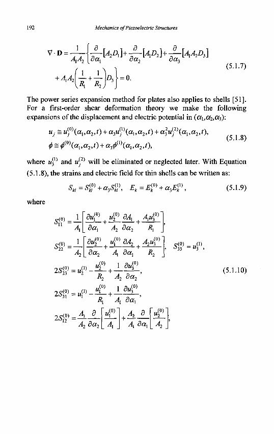
192 Mechanics of Piezoelectric Structures
V D AA
8 kA]+-/-kA]+^-tW>3] da, da-, da-,
+ AXA2 1 1
• + •
(5.1.7)
V*> R A =°-• 2 /
The power series expansion method for plates also applies to shells [51]. For a first-order shear deformation theory we make the following expansions of the displacement and electric potential in {a\,a2,a^):
Uj = u(f\al ,a2,t) + ajjlf (ax ,a2,t) + a%uf* (ax, a2, t),
0 = 0(O)tei,a2»O + a30(1)(ai,a2,O»
where u^ and «j2) will be eliminated or neglected later. With Equation
(5.1.8), the strains and electric field for thin shells can be written as:
(5.1.8)
Su=W + a3s2\ Ek=Et» + a3E?\ (5.1.9)
where
4P--L du[0) | i40) 3AX ^ A,u\
dal
(0) 3
C(0) _ °22 -
1
A2 da2 R
di / f u\u> dA2
——+ — - + da2 Ax da,
i/°) 1 d j / 0 )
vi
R,
AW(°)
R, A2 da2
iy(°) 1 r)nm
" 3 3 — M 3 '
25w=A_L 42 d«2
,(°) + 4 a ^i 5a,
«£0)
(5.1.10)
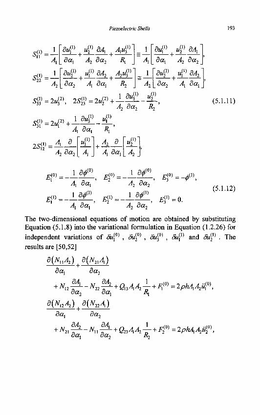
Piezoelectric Shells 193
5ff
e ( i ) _ °22 -
M y , «41} a * , ^ 9a, -42 9or2 i?,
9wl W, ——+ da-,
1 ^ * 2 , ^ 2 M 3
yi, 9 ^ & : 4
9w,(1) M: —— + da,
_£>94 A2 da2
du?
da-,
,(!)
+ -dA,
Ax dax
S^=2uf\ 2S$ = 2u™+ 1 ^ A2 da2
(5.1.11)
5,iI1> = 2 t t [ 2 ) + 1
A
i c ( D _ 4 5
12 — J 2 3a2
9«« dax
k ( 1 ) l .4.
Wl(1)
A2 9
4, 9a,
4, 9a,
ft") - * 9<*(1)
. F.m=-
_A2_ ?
1 9<*(0)
v42 9 a 2
1 9 0<*>
£f -r, (5.1.12)
Ax dax A2 da2
E{1)=0.
The two-dimensional equations of motion are obtained by substituting Equation (5.1.8) into the variational formulation in Equation (1.2.26) for
independent variations of Suxm , <5w2
0) , duf^ , Suxm and Su^ . The
results are [50,52]
3 ( t f n 4) + _a ( t f 2 1 4)
da, da,
+ Nn^-N22^ + QuAxA2±- + Fr =2PhAxA2u?\ da2 dax /?,
d{NX2A2) + d(N22Ax)
da, da-,
dA dA + N2X-±-Nxx-± + Q23AxA2 — + F2m =2phAxA2u?)
da, da R,
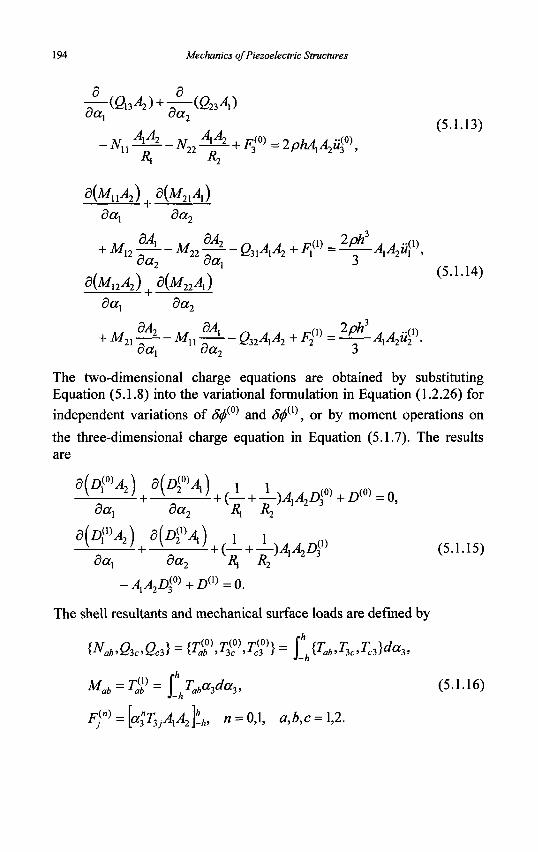
194 Mechanics of Piezoelectric Structures
8 (Q34)+-A(&34) da, oa7 2 (5.1.13)
-Nn^-N22^ + F^ =2PhAxA2uf\
d(MuA2) f d{M2lAx)
dax da2
+ Mn %L _ M22 ^ - Q3lAA2 + F{" = ^-AXA2^\ oa7 da, 3
(5 1 14) 5(M,2^2) | d{M22Ax)
9a, 9a2
+ M21 %L - Mn P- - Q3lAA2 + F" = ^AXA2$\ aax da2 3
The two-dimensional charge equations are obtained by substituting Equation (5.1.8) into the variational formulation in Equation (1.2.26) for
independent variations of 8<j>^ and Stf>m, or by moment operations on
the three-dimensional charge equation in Equation (5.1.7). The results are
d(E&0)A,) d(D^A) 1 1
dax da2 i?, R2
d(D^A2) d(D?A) 1 1 V 2 > + V 1/ + (_L + _L)j i^Zj(i) (5.1.15) da, 9a2 /?] i?2
-AA2D^+D^=0.
The shell resultants and mechanical surface loads are defined by
W*.03o0C3} = { ^ M c W ) = ?h{Tab,T3c,Tc3}da3,
Mab=TV = \h_hTaba3da3, (5.1.16)
^j"> = [ 0 ^ , 4 4 ] ^ , /i = 0,1, a,b,c = \,2.
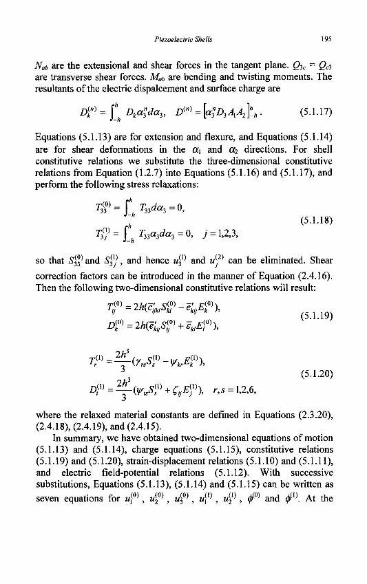
Piezoelectric Shells 195
Nab are the extensional and shear forces in the tangent plane. Q^c = Qc3
are transverse shear forces. Mab are bending and twisting moments. The resultants of the electric dispalcement and surface charge are
DP = \[h Dka"3da3, Dw = \a"3D3AxA^h • (5-1-17)
Equations (5.1.13) are for extension and flexure, and Equations (5.1.14) are for shear deformations in the a,\ and a-i directions. For shell constitutive relations we substitute the three-dimensional constitutive relations from Equation (1.2.7) into Equations (5.1.16) and (5.1.17), and perform the following stress relaxations:
*%-t T33da3 = 0, * (5.1.18)
TV=L T33a3da3 = 0, 7 = 1,2,3,
so that S$ and Sy , and hence u3l) and u^p can be eliminated. Shear
correction factors can be introduced in the manner of Equation (2.4.16). Then the following two-dimensional constitutive relations will result:
T^=2h(crklSJ»-e^\
D^ = 2Ke'kijS^ + sklE^), (5.1.19)
DV^iy^+^Ef), r,s = 1,2,6,
(5.1.20)
where the relaxed material constants are defined in Equations (2.3.20), (2.4.18), (2.4.19), and (2.4.15).
In summary, we have obtained two-dimensional equations of motion (5.1.13) and (5.1.14), charge equations (5.1.15), constitutive relations (5.1.19) and (5.1.20), strain-displacement relations (5.1.10) and (5.1.11), and electric field-potential relations (5.1.12). With successive substitutions, Equations (5.1.13), (5.1.14) and (5.1.15) can be written as
seven equations for w,(0) , u^ , w<0) , w,(1) , u(? , (jf0) and 0(1). At the
196 Mechanics of Piezoelectric Structures
Nm
Mnn
£(0)
or
or
or
w(0)
u?, ^ 0 \
Nns
Mm
D?
or
or
or
M(0) "s '
"s '
f\
boundary of a shell with a unit exterior normal n and a unit tangent s, we may prescribe
Q% or <>,
(5.1.21)
Equations for laminated piezoelectric shells can be found in [53]. Equations for electroelastic shells under biasing fields can be found in [54,55] along with buckling analysis [55]. Nonlinear equations for electroelastic shells in large thickness-shear deformations can be found in [56].
5.2 Classical Theory
For the classical theory of a shell in coupled extension and flexure without shear deformations, we set the relevant shear strains to zero:
R, A, da, 1 ' ' (5.2.1)
R2 A2 da2
This allows us to express w,(1) and u^ in terms of the zero-order displacements for extension and flexure. Furthermore, we ignore the rotatory inertia in Equation (5.1.14) and obtain
d(MuA2) ( 3 ( M 2 1 4 )
dax da2
+ Mn^-M12^-Q,XAA1+FV=Q, oa2 oax
d(Ml2A2) ( d(M22Ax)
dax da2
+ M2l^-Mu-^-Q32AA2+F2V=0, oax oa2
(5.2.2)
Piezoelectric Shells 197
which yields expressions for transverse shear forces Q3i and Q32 in terms of the bending and twisting moments. In summary, the equations for the classical theory are
d(NnA2) | d{N2XAx)
dax da2
+ *l2P-N22f^ + QUAXA2±- + Fr = 2phAxA2^\ oa2 oax Rx
d(NX2A2) ( d(N22Ax)
dax da2
^N2X^--Nn^ + Q23AXA2 - L + F? > = 2 p W , ^ 0 ) ,
/-(a34)+^-(fi23^.) a«! oa2
_ JVU M . _ M . + F3(°) = 2pfe4^ii! ,(0)
Kx K2
where
d(p^A2) t d(p^Ax)
dax da2
d(pfl2) | 2d{D?Ax)
dax da2
Hj + y)AA2pV-AxA2pM+pV=0,
N^ =2h{c'rsS^-e'krEf\
Pf^lKelS^+EyEf), r,s = 1,2,6,
(5.2.3)
(5.2.4)
(5.2.5)
Mechanics of Piezoelectric Structures
W-lyiV^ + Stfh r,* = 1A6, (5.2.6)
QiAAi „ MnA) , 9 (^2 i4 ) 5«,
+ M, 94
- M , 12 - J " 2 2 0 « T da,
da-,
+Fii\
n A A d(MuA) , d(Mzt4) 9a, 9a,
+ ^21 -r-^—Af,,—!- + F?\ dax oa2
(5.2.7)
*K du[0) Mf 94 4«f
e(0) _ 1 j 22
9a, ^2 da2 ^1
"&40) », ( 0 )9^2 , ^ i 4 0 ) ' 9a, J, 9a, &
42 9a2
,/o)
4 + A2 9
v4, 9a ,
./»)
(5.2.8)
sff -
c(l) -^22 "
c ( l ) . 0,2 -
1
''A 1
= J 2
~9w,(1) M21} 9 4 "
9a , 42 da2
~du(2l) u^ dA2
da2 Ax dax
_AX 9
^42 9a 2
~uf A
5
5
+ A d Ax dax
"i41)"
4
(5.2.9)
Piezoelectric Shells 199
,.(0) i a,.(0) ( 1 ) _ W, 1 OU3
U\ — ,
(1) *40) 1 du{0)
« 2 = •
(5.2.10)
R2 A2 da2
*(°> ... 1 ^ < ° )
*f».~I$£. *?>—L*£. »=o. -4 da, A2 da2
.0)
(5.2.11)
With successive substitutions, Equations (5.2.3) and (5.2.4) can be written as five equations for w[0) , w2
0) , u^ , 0(O) and </>m. At the boundary of a shell with unit exterior normal n and unit tangent s, we may prescribe
TV or w(0) iV or «(0)
Q^ + M^ or uf\ M„„ or «g>, (5.2.12)
Z>(°> or ^(0), 0<'> or <*(1).
5.3 Membrane Theory
A thin piezoelectric shell can sometimes be treated as a membrane that does not resist bending, without bending moments and transverse shear forces. In this case we have the following membrane theory:
aax oa2 oa2 oax
oax oa2 oax da2
-Nu±-N*+F}<»=2phu?\
200 Mechanics of Piezoelectric Structures
d(D^A2) d(D^Ax) , i - -i—ii + _Li_ii + (_L + _L)^2 j D(o) +jD(0) = 0,
dax da2 I\ R2
d(D^A2) dlD^AA ! !
da, - + - 6a-, ^ ^ 2
- 4 ^ 0 ) + Z ) ( 1 ) = 0 ,
(5.3.2)
D ^ / ^ S ^ + ^ ' X r,s = 1,2,6, (5.3.3)
Dl id) 2/*3 <i) s E(}
bij^j ' (5.3.4)
«P=i o(0) _ J _ °22 ~ ^
2S|20 )
a»,(0) i4°> 54 M0)
da, A2 da2
XL + 3 " 3
ft
d»f + t^_a4+£2Mf da2 Ax dax R2
Ax d
A2 da2
" M l( 0 > " A2 d
Ax dax
(5.3.5)
E } 0 ) = -
£?>=•
,(°) 1 dtp
Ax dax
1 d<f>m
Ax dax
E™
E$>
1 d ^
42 5 a 2
1 <ty(1)
J 2 3 a 2
E^ = -f\
&=0.
(5.3.6)
With successive substitutions, Equations (5.3.1) and (5.3.2) can be
written as five equations for w,(0) , w20) , u\0) , <jf0) and <jfl\ At the
boundary of a shell with a unit exterior normal n and a unit tangent s, we
may prescribe
,/°) i,(°) N or u ' N or u(
iv m u i un , jy m u i us ,
a (0) or <F\, E%> or ^ ,(i) A(D
(5.3.7)
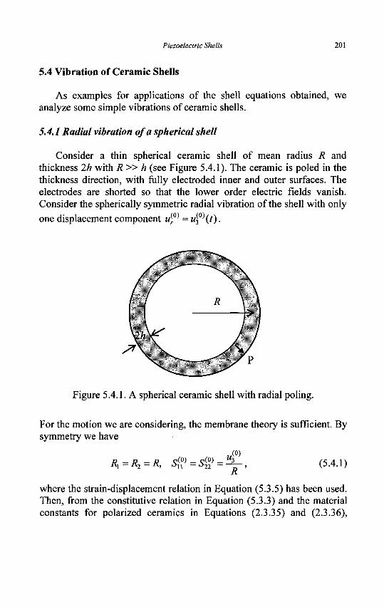
Piezoelectric Shells 201
5.4 Vibration of Ceramic Shells
As examples for applications of the shell equations obtained, we analyze some simple vibrations of ceramic shells.
5.4.1 Radial vibration of a spherical shell
Consider a thin spherical ceramic shell of mean radius R and thickness 2h with R» h (see Figure 5.4.1). The ceramic is poled in the thickness direction, with fully electroded inner and outer surfaces. The electrodes are shorted so that the lower order electric fields vanish. Consider the spherically symmetric radial vibration of the shell with only
one displacement component M£0) = u^°\t).
Figure 5.4.1. A spherical ceramic shell with radial poling.
For the motion we are considering, the membrane theory is sufficient. By symmetry we have
„(0)
R^R2=R, 5<»>=5g>=fi- , (5-4.1) R
where the strain-displacement relation in Equation (5.3.5) has been used. Then, from the constitutive relation in Equation (5.3.3) and the material constants for polarized ceramics in Equations (2.3.35) and (2.3.36),
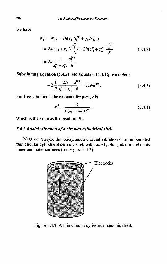
202 Mechanics of Piezoelectric Structures
we have
Nn=Nn=2h(rnS<» + r12S$>)
M ( 0 ) 7 i ( 0 )
= 2h 1 ,/°) 4+4 R
Substituting Equation (5.4.2) into Equation (5.3.1)3, we obtain
R4+4 R p 3 • For free vibrations, the resonant frequency is
2 2 (° = V U 1~>
P(5f,+4)i?2
which is the same as the result in [9].
5.4.2 Radial vibration of a circular cylindrical shell
(5.4.2)
(5.4.3)
(5.4.4)
Next we analyze the axi-symmetric radial vibration of an unbounded thin circular cylindrical ceramic shell with radial poling, electroded on its inner and outer surfaces (see Figure 5.4.2).
* 2
Electrodes
Figure 5.4.2. A thin circular cylindrical ceramic shell.
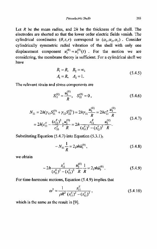
Piezoelectric Shells 203
Let R be the mean radius, and 2h be the thickness of the shell. The electrodes are shorted so that the lower order electric fields vanish. The cylindrical coordinates (6,z,r) correspond to (aua2,a3) . Consider cylindrically symmetric radial vibration of the shell with only one displacement component (f) . For the motion we are considering, the membrane theory is sufficient. For a cylindrical shell we have
AX=R, A2 = \.
The relevant strain and stress components are
M(0) w ( 0 )
(cEf um sE w (0 )
33 R (^)2-(4)2 & - 2h\cE - K UJ 1 3 - 2/z
Substituting Equation (5.4.7) into Equation (5.3.1)3
we obtain
For time-harmonic motions, Equation (5.4.9) implies that
, 2 = 1
pR2(sW-(S?2f which is the same as the result in [9].
(5.4.5)
•C=4r ' ^ } =0 , (5.4.6) K
(5.4.7)
-Nnj = 2pMf\ (5.4.8)
-^MA^If2^' (5A9) c^ii) - ( ^ i 2 ) •« ^
® - - S T ^ T T T ' (5-4-10>
204 Mechanics of Piezoelectric Structures
5.5 A Shell on a Non-Thin Body
In some applications, we have a thin layer of one material on the surface of a body of another material. Such a structure can be modeled as a two-dimensional shell on a three-dimensional body with interface continuity conditions.
5.5.1 A piezoelectric shell on an elastic body
Consider static deformations of an elastic body coated with a thin piezoelectric film [57].
5.5.1.1 Governing equations
The piezoelectric shell has the following material matrices under the compact matrix notation:
e2i e22
_ei\ e32
As special cases, the matrices in Equation (5.5.1) include piezoelectric ceramics poled in the 1, 2, or 3 directions. The shell is assumed to be very thin so that the membrane theory is sufficient. The membrane tensile and shear forces and electric displacements are given by the following constitutive relations:
M2
Cl3
0
0
0
°12
C22
C23
0
0
0
•-13
C23
C33
0
0
0
0 0 0 0
0 C44
0
0
0
0
C55
0^ 0 0
0
0 c66y
-23 c24
c15
c25
c16
c26 512 '22 "23 (5.5.1)
c33 "34 c36_ = 13 '23 533
Piezoelectric Shells 205
Nxx = NX = 2h(c[xSxw + c(A0) ~ e£A0)),
N22 = N2 = 2h{cxp
2S\Q) + cp22S
{2
0) - ep2E^\
Nu=N6=2h(c66Si0)-ek6Ei0)),
D™ = 2h{e^ + ep2S^ + eufl> - epE™),
(5.5.2)
where
c l l = c l l _ C 1 3 ' C 3 3 5 C12 = c12 _ C 1 3 C 3 2 ' C 3 3 '
C22 = C 2 2 _ C 2 3 ' C 3 3 > g i l ~ ek\ ~C\3ek3' C33' ( 5 . 5 . 3 )
ek2 = ek2 ~ C23ek3 ' C 33 ' £kl = £kl ~ ek3el3 ' C33 •
The membrane equations of equilibrium and electrostatics take the form
d (A2Nx) + ^-(AxN6)
h
dax da2
BA BA
oa2 oax "
-^(A2N6) + ^-(AxN2) oax oa2
BA BA h + N2-Ni+AlA2(2phf2+T32\
hh) = 0, (5.5.4)
oax Ba2 "
- ^ - N 2 ^ + 2phf3+Ti3\h_h=0,
Kx K2
9 (A2DX^) + ^(AXD^) 8ax 8a2
+ (± + l-)AxA2D^ + AxA2Dlh=0. Rx R2
With successive substitutions from Equations (5.5.2), (5.3.5) and (5.3.6), Equations (5.5.4)j.3 can be written in the following compact form:
Lp{v?>Jw,P>) + 2pkffi+t+fi-rfi=0, (5.5.5)
206 Mechanics of Piezoelectric Structures
where Lp are linear differential operators, and t% = T3 „ (±h) are the
traction vectors at the major faces of the film. /? = 1, 2, 3 is associated with the shell principle coordinates (a.\, a2, a^). At every point of the shell, there exists a set of transformation coefficients 3$ between the local shell principal coordinates and the global Cartesian coordinates. Multiplying Equation (5.5.5) by the transformation coefficients, we have
Z,(u<V W 2 p & / , +t! -t~ = 0. (5.5.6)
The elastic body is governed by the equations of linear elasticity.
5.5.1.2 Boundary integral equation formulation
Since the film interacts with the body through the surface of the body, we use the boundary integral equation (BIE) formulation and its numerical solution technique - the boundary element method. The displacement u and surface traction t of the elastic body (in a domain Q with boundary T) satisfy the following boundary integral equation:
C(J>0)u(/>0) + f T(7»,/>0)u(iW/»)
f - f - ( 5 - 5 J )
= V(P,PQ)t(P)aT(P) + j V(P,P0)b(P)dQ(P), •T •'£2
where Cy = 6y/2 for a smooth boundary, b is the body force vector of the elastic body, U and T are known second rank tensors and are related to the fundamental solution of the Navier operator in elasticity. They can be found in a book on boundary element method in elasticity. P is the source point and P0 is the field point. The traction vector t on the surface of the elastic body is related to the traction on one of the faces of the film
by t = -t~ . Therefore, from Equations (5.5.6) and (5.5.7), we obtain [57]
Cu+ f JuaT = - \ ti(L + 2phf + t+)dT+ f UbrfQ, (5.5.8) Jr Jr Jn
where the displacement continuity conditions between the body and the film have been used. Equation (5.5.8) is a system of boundary integral-differential equations because of the differential operator L. If the body is only partially coated with a film, then BIE (5.5.7) applies to the non-coated portion of the surface.
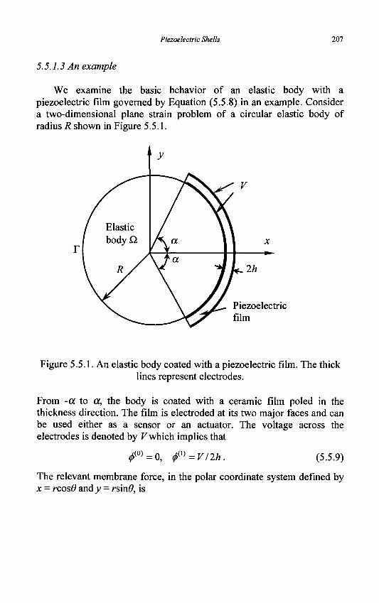
Piezoelectric Shells 207
5.5.1.3 An example
We examine the basic behavior of an elastic body with a piezoelectric film governed by Equation (5.5.8) in an example. Consider a two-dimensional plane strain problem of a circular elastic body of radius R shown in Figure 5.5.1.
Figure 5.5.1. An elastic body coated with a piezoelectric film. The thick lines represent electrodes.
From -a to a, the body is coated with a ceramic film poled in the thickness direction. The film is electroded at its two major faces and can be used either as a sensor or an actuator. The voltage across the electrodes is denoted by V which implies that
/°>=0, f^Vllh. (5.5.9)
The relevant membrane force, in the polar coordinate system defined by x = rcosO and y - rsin#, is
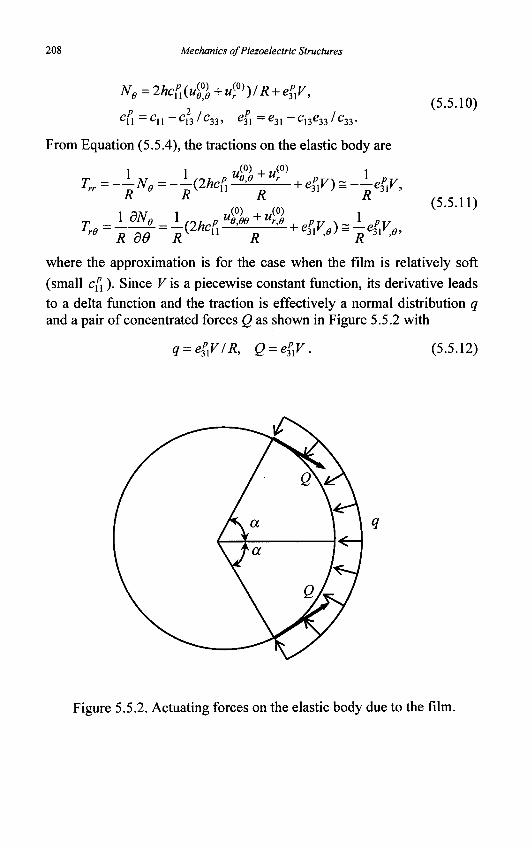
208 Mechanics of Piezoelectric Structures
Ng=2hc?l(u™+u<?))IR + e*xV,
C, i = C\ i — C n / C->\, &w = 6-11 — C\\(Z%% I C%
(5.5.10) -"13 ' ^ 3 3 ' c31 c31 - 1 3 c 3 3 ' u 3 3 -
From Equation (5.5.4), the tractions on the elastic body are
i i „4V"0 )
^ 0 ^ v i i R + ep
lV) = ~epiV,
K
lr6 R dd
1 —(2hrp Ue'ee ^-£- + ppV \^—PPV R\AnCU „ +e3V,e)- R
e3V,6>
(5.5.11)
where the approximation is for the case when the film is relatively soft (small cxl). Since V is a piecewise constant function, its derivative leads to a delta function and the traction is effectively a normal distribution q and a pair of concentrated forces Q as shown in Figure 5.5.2 with
q = epxV/R, Q = ep
xV (5.5.12)
Figure 5.5.2. Actuating forces on the elastic body due to the film.
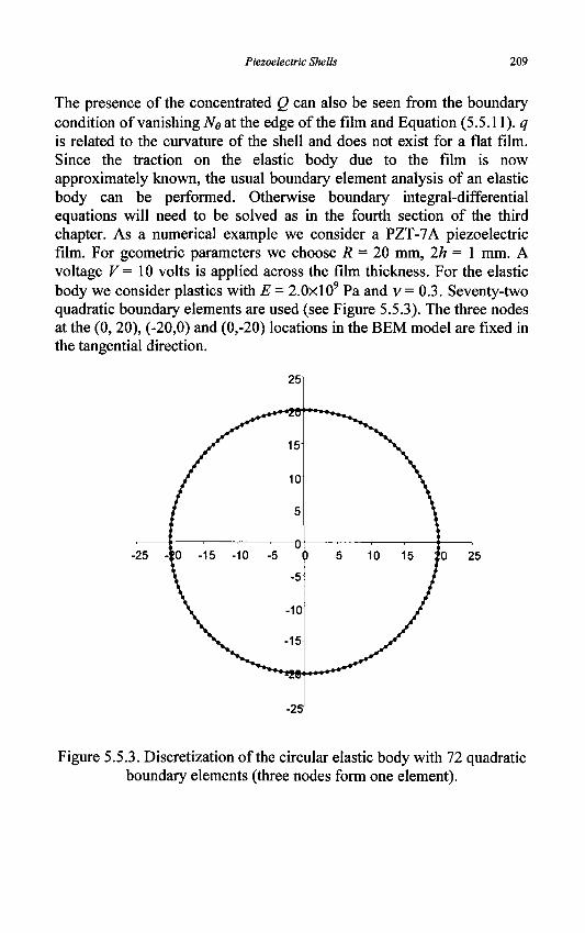
Piezoelectric Shells 209
The presence of the concentrated Q can also be seen from the boundary condition of vanishing Ne at the edge of the film and Equation (5.5.11). # is related to the curvature of the shell and does not exist for a flat film. Since the traction on the elastic body due to the film is now approximately known, the usual boundary element analysis of an elastic body can be performed. Otherwise boundary integral-differential equations will need to be solved as in the fourth section of the third chapter. As a numerical example we consider a PZT-7A piezoelectric film. For geometric parameters we choose R = 20 mm, 2h = 1 mm. A voltage V = 10 volts is applied across the film thickness. For the elastic body we consider plastics with E = 2.0x10⁹ Pa and v = 0.3. Seventy-two quadratic boundary elements are used (see Figure 5.5.3). The three nodes at the (0, 20), (-20,0) and (0,-20) locations in the BEM model are fixed in the tangential direction.
Figure 5.5.3. Discretization of the circular elastic body with 72 quadratic boundary elements (three nodes form one element).
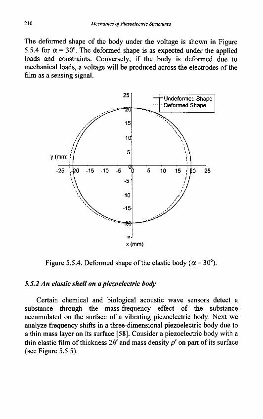
210 Mechanics of Piezoelectric Structures
The deformed shape of the body under the voltage is shown in Figure 5.5.4 for a = 30°. The deformed shape is as expected under the applied loads and constraints. Conversely, if the body is deformed due to mechanical loads, a voltage will be produced across the electrodes of the film as a sensing signal.
x(mm)
Figure 5.5.4. Deformed shape of the elastic body (a = 30°).
5.5.2 An elastic shell on a piezoelectric body
Certain chemical and biological acoustic wave sensors detect a substance through the mass-frequency effect of the substance accumulated on the surface of a vibrating piezoelectric body. Next we analyze frequency shifts in a three-dimensional piezoelectric body due to a thin mass layer on its surface [58]. Consider a piezoelectric body with a thin elastic film of thickness 2h' and mass density p ' on part of its surface (see Figure 5.5.5).
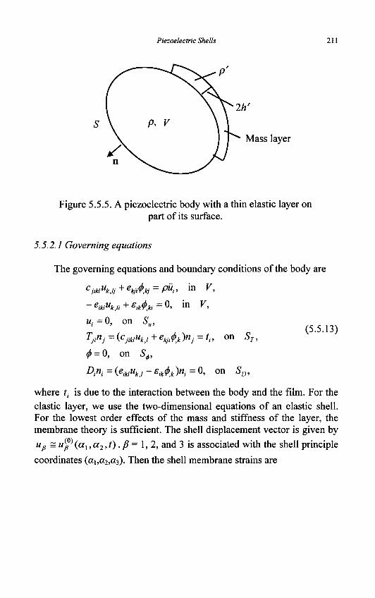
Piezoelectric Shells 211
Figure 5.5.5. A piezoelectric body with a thin elastic layer on part of its surface.
5.5.2.1 Governing equations
The governing equations and boundary conditions of the body are
cjikiukjj + ekAkj = pUi, in V,
-eikiuk,ii+eik<t>M=^ i n F ' w,=0, on Su, Tjinj = (cjikiuk,i + ekAk )nj = *„ o n ST .
<j> = 0, on Sp
where ^ is due to the interaction between the body and the film. For the elastic layer, we use the two-dimensional equations of an elastic shell. For the lowest order effects of the mass and stiffness of the layer, the membrane theory is sufficient. The shell displacement vector is given by
Up = u^P(al,a2,t). p = 1,2, and 3 is associated with the shell principle
coordinates {a\,a2,a^). Then the shell membrane strains are
(5.5.13)
212 Mechanics of Piezoelectric Structures
rf0) _ l du^ t » f dAx | 1 ^
, , ,=±Mi + j f ^ + ±„<.> (5 .5 ,4) -42 9a2 V4,Y42 9a, R2
AO) _iA ( i ! ) + AA ( f 4 9a, At A-, da-, A,
The membrane stress resultants are given by the following constitutive relations:
N^lhXrnS^ + rnS^),
N2=2h'(ruSl0) + riA0)), (5.5.15)
N6=2h'y66Sf).
The membrane equations of motion are
9 (A2Nx) + ^-(AxN6) dax da2
+ N ^ - N 2 ^ + AxA2fx = AxA22pWu?\ oa2 oax
-^-(A2N6) + ^-(AxN2) (5.5.16) oax oa2
+ N6^-Nx^- + AxA2f2 = AxA22p'h'uf\ oax oa2
-jNx-j-N2 + f3 = 2p'h'u<?\
where / is the load per unit middle surface area of the shell. With successive substitutions, Equation (5.5.16) can be written in the following compact form
-LfS(u(0)) + fp=2p'h'uf, (5.5.17)
where Lp are linear differential operators. Multiplying Equation (5.5.17) by the transformation coefficients S,p between the local shell principal coordinates and the global Cartesian coordinates, we have
-A(n ( 0 ) ) + // =p'h'ufK (5.5.18)
Piezoelectric Shells 213
We note that the /, in Equation (5.5.13)4 and the ft in Equation (5.5.18) are actions and reactions, equal in magnitude and opposite in direction (ft = -'/)• Substituting Equation (5.5.18) into Equation (5.5.13)4, for time-harmonic motions with an exp(zorf) time dependence, the eigenvalue problem for the free vibration of the body with the film can be written as
-cjikiuk,ij-ekAkj=pAun i n V,
-eikiukji+£ik^ki=0, in V,
ut=0, on Su,
TPnJ = (cjikiuk,i + ekjih>j (5.5.19)
= £[2p'h'/luj-Lj(u)], on ST,
<f> = 0, on Sj,
A",=(eikiuk,i - ^ , * H = 0 , on SD,
where we have denoted X = a>2. e is a small parameter introduced to formally show the smallness of the effect of the film. The real physical problem corresponds to e = 1. Because of the continuity between the
layer and the body, the displacement of the layer u(0) is the same as the displacement u of the piezoelectric body at its surface S. Equation (5.5.19) can be written in a more compact form as
AU = ABU, in V,
ut=0, on Su,
TJi(VynJ=e[2p'h'*ul-Li(u)]„ on ST, (5.5.20)
^ = 0, on S+,
0,(11)71, =0, on 5-D,
where U = {uk,<p} is a 4-vector. The differential operators A and B are defined by
AU = {-cJikluklj-ekjl<f>kJ-eiklukli+£Ul<f>ki}, (5.5.21)
BV = {pui,0}.
7},(U) and A(U) are the stress tensor and electric displacement vector in terms of the 4-vector.
214 Mechanics of Piezoelectric Structures
5.5.2.2 Perturbation analysis
We look for a perturbation solution to Equation (5.5.20). Consider the following expansions:
= U(0) + £U(1),
where and ^(0) are the frequency and modes when the elastic layer is not present. Beginning from Equation (5.5.22), for the rest of this section, the superscripts will be for perturbation orders, not for orders of shell displacements. Substituting Equation (5.5.22) into Equation (5.5.20), collecting terms of equal powers of e, we obtain a series of perturbation problems of successive orders. We are interested in the lowest order effect of the layer. Therefore we collect coefficients of terms with powers of e° and e1 only. The zero-order problem is
-cm$l-eJ$=p&W, in V, - e « « ^ + ^ 0 ) = 0 , in V,
«,(0) = 0, on Su,
(cJiklu<i!>] + ekJi^)nJ=0, on ST,
^(0) = 0, on S+,
(e^J-eJ^yn^O, on SD.
(5.5.23)
This represents free vibrations of the body without the surface mass layer. The solution to the zero-order problem, A(0) and U(0), is assumed known as usual in a perturbation analysis. The first-order problem below is to be solved:
Piezoelectric Shells 215
- c « 4 ! ) / + ^ ) = 0 , in K,
w,(1)=0, on Su, (5 5 24)
(c^«i1j + ^J ))n>=[2p%U ( 0 ) i |W-Z I . (nW)], on ST,
<*(1)=0, on S,,
( « a / 4 ! K ^ ( * ) K = 0 , on 5-D.
The differential equations for the first-order problem, Equations (5.5.24)12, can be written as
AU(1) = A(0)BU(1) + A(I)BU(0). (5.5.25)
Multiplying both sides of Equation (5.5.25) by U(0) and integrating the resulting equation over V, we have
<AU (1);U (0)>
= I [(-CjiAl ~^i<r§)^0) H - e ^ + e ^ ^ W (5-5.26)
- A(0) < BU(1);U(0) > +Am < BU(0);U(0) >,
where, for simplicity, we have used < ; > to represent the product of two 4-vectors and the integration over V. With integration by parts, it can be shown that
<AU (0);U (1)>
= - J [Tj, (U(0) )njuf) + D, (U(0) )n^m ]dS . S (5.5.27)
+ £ [Tkl(Vm)n,u^+Dk(V^)nk^]dS
+ <U (0 );AU (1 )>.
With the boundary conditions in Equations (5.5.23)3.6 and (5.5.24)3.6, Equation (5.5.27) becomes
<AU (0);U (1)>
= J [Ip'h'^u^ - Lk(um)]u(
k0)dS+ < U(0); AU ( 1 ) > (5.5.28)
(5.5.29)
216 Mechanics of Piezoelectric Structures
Substituting Equation (5.5.28) into Equation (5.5.26),
< AU(0);U(1) > - f [2p'h'X%^ - 4(u ( 0 ) ) ]4 0 ) ^
= X0) < BU(,);U(0) > +Am < BU(0);U(0) >,
which can be further written as
<AU ( 0 ) - i 0 ) BU ( 0 ) ;U ( 1 ) >
- J [2p%'A(0)«f)-Z t(u(0))]«f)dS (5.5.30)
= ^ 1 ) <BU ( 0 ) ;U ( 0 ) >.
With Equations (5.5.23)i2, we obtain, from Equation (5.5.30)
i(l) _ _ JST
<BU<°>;U<°>> (5.5.31)
Ipuf^dV
The above expression is for the eigenvalue A, = a1. For a> we make the following expansion:
ca = (o(0)+E(Dm. (5.5.32)
Then
Hence
sa>m 1
(5.5.33)
«<»> ~ 2(comf B&>
1 -sJS f [2p'h'^u^-Lk(u
m)]uk0)dS (5-5-34)
JST
2(«(0))2 \pu™u™dV
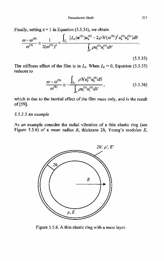
Piezoelectric Shells 217
Finally, setting e= 1 in Equation (5.5.34), we obtain
a-d* 1 is [4(«(0))40)-2^V0))240)40)]^ a>m ~2(a/ 0 ) ) 2 \vP^dV
(5.5.35)
The stiffness effect of the film is in Lk. When Lk = 0, Equation (5.5.35) reduces to
0)-C0 (0)
CO ,<°)
J p'h'uf^dS
)vPu^dV ^ (5.5.36)
which is due to the inertial effect of the film mass only, and is the result of [59].
5.5.2.3 An example
As an example consider the radial vibration of a thin elastic ring (see Figure 5.5.6) of a mean radius R, thickness 2h, Young's modulus E,
2h',p',E'
Figure 5.5.6. A thin elastic ring with a mass layer.
218 Mechanics of Piezoelectric Structures
Poisson's ratio v, and mass density p. The mass layer has a thickness 2h\ Young's modulus E' and mass density p'.
A ring can be considered as a circular cylindrical shell with the axial extensional force Nz = 0. When the mass layer is not present, in cylindrical coordinates, the lowest radial mode is given by ([9] or Equation (7.3.6) of the present book)
t«»v> (*>w) *v .,«» = C, .,«» = 0, , ( ° > - c
(5.5.37)
= -v—z = 0, R
where C is an arbitrary constant. u™ is due to Poisson's effect, which is relatively small and is neglected as an approximation. For the layer, the equation of motion in the radial direction is
2h'E'
R2 -ur+fr = 2p'h'ur.
Hence
400 = 2h'E'
R2 ur, Le(u) = 0, 4 ( u ) = 0.
(5.5.38)
(5.5.39)
Substituting Equations (5.5.37) and (5.5.39) into the perturbation integral in Equation (5.5.35), we obtain the frequency shift due to the mass layer as
co-co ,("> 1 1 CO
(0) -2(com)22ph
1 1
2h'E'
R2 -2p'h'(o){0))2
2(co{0))2 ph
2h\E
(h'E' Py E
R' R2p, (5.5.40)
P_
PJ
Equation (5.5.40) shows that the inertial effect of the mass layer lowers the frequency, and the stiffness of the mass layer raises the frequency as expected. The result of Equation (5.5.40) and the result from [59] considering the inertial effect of mass only (which is the special case of
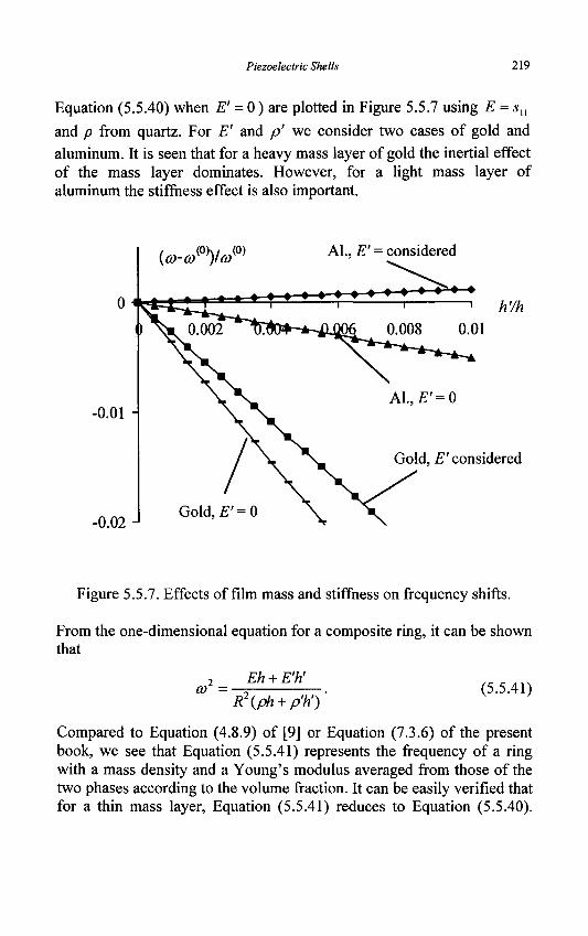
Piezoelectric Shells 219
Equation (5.5.40) when E' = 0) are plotted in Figure 5.5.7 using E = su
and p from quartz. For E' and p' we consider two cases of gold and
aluminum. It is seen that for a heavy mass layer of gold the inertial effect of the mass layer dominates. However, for a light mass layer of aluminum the stiffness effect is also important.
Figure 5.5.7. Effects of film mass and stiffness on frequency shifts.
From the one-dimensional equation for a composite ring, it can be shown that
2 Eh + E'h' ,ecAK GO =—-z . (5.5.41)
R2{ph + p'h') Compared to Equation (4.8.9) of [9] or Equation (7.3.6) of the present book, we see that Equation (5.5.41) represents the frequency of a ring with a mass density and a Young's modulus averaged from those of the two phases according to the volume fraction. It can be easily verified that for a thin mass layer, Equation (5.5.41) reduces to Equation (5.5.40).
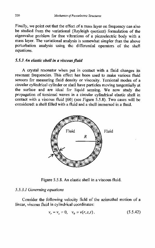
220 Mechanics of Piezoelectric Structures
Finally, we point out that the effect of a mass layer on frequency can also be studied from the variational (Rayleigh quotient) formulation of the eigenvalue problem for free vibrations of a piezoelectric body with a mass layer. The variational analysis is somewhat simpler than the above perturbation analysis using the differential operators of the shell equations.
5.5.3 An elastic shell in a viscous fluid
A crystal resonator when put in contact with a fluid changes its resonant frequencies. This effect has been used to make various fluid sensors for measuring fluid density or viscosity. Torsional modes of a circular cylindrical cylinder or shell have particles moving tangentially at the surface and are ideal for liquid sensing. We now study the propagation of torsional waves in a circular cylindrical elastic shell in contact with a viscous fluid [60] (see Figure 5.5.8). Two cases will be considered: a shell filled with a fluid and a shell immersed in a fluid.
Figure 5.5.8. An elastic shell in a viscous fluid.
5.5.3.1 Governing equations
Consider the following velocity field of the azimuthal motion of a linear, viscous fluid in cylindrical coordinates:
vr = v z =0, ve = v(r,z,t). (5.5.42)
Piezoelectric Shells 221
The nontrivial stress components are [61]
or
dfv^
\rJ Trz = M—.
oz (5.5.43)
where n is the viscosity of the fluid. The relevant equation of motion is [57J
A-H dt
M 1 o v Idv
+ — + M <L1 dz2
(5.5.44) ^drz r dr
where p' is the fluid density. We look for a wave solution in the form
v = V(r) sin kzexp(icot), (5.5.45)
where k is the wave number and co is the frequency. Substitution of Equation (5.5.45) into Equation (5.5.44) results in the following equation forF:
d2V 1 dV
d? <rs<r i+
i v = o.
where
M
(5.5.46)
(5.5.47)
Equation (5.5.46) is the modified Bessel equation of order one. Its general solution is a linear combination of I\(Xr) and K\(Xr), the first order modified Bessel functions of the first and second kind. Hence
v = \CxIx(fo) + CjK^Ar^sinkzexpiioX), (5.5.48)
where C\ and C2 are undetermined constants. Consider torsional motions of a circular cylindrical shell with
thickness 1h and middle surface radius R. The membrane theory is sufficient. Let the middle surface displacement field be
« i u, ,(0)
u
,(0) 1
, ( 0 ) _ M ( 0 )
(0) _ ,,(0) _ uy =u,
u(z,t),
0,
0.
(5.5.49)
222 Mechanics of Piezoelectric Structures
From Equation (5.3.1)! the equation that governs u is
plhu = G 2 A | 4 +TrB (R+) -Trd (R~), dz
(5.5.50)
where n is the mass density and G is the shear modulus of the shelL TrB(R+) and Trd(R~) are the shear stress components at the outer and inner surfaces of the shell. They are due to the interaction with the fluid.
Substituting Equation (5.5.43) into Equation (5.5.50) we have
p2hii = G2h— + 'dz2
JM (5.5.51)
Differentiating Equation (5.5.51) with respect to time once, using the continuity of velocity (non-slip condition) between the shell and the fluid, we obtain
p2hv\R = G2h— dz +
R+ L
jjr 3 fvA dr \ r MR-
(5.5.52)
5.5.3.2 Interior problem
First consider a circular cylindrical shell filled with a fluid (interior problem). In this case, for the fluid region, since K^O) is unbounded, we must have C2 = 0 in Equation (5.5.48). Substituting the remaining C\ term into Equation (5.5.52), we obtain
2 2 , 2 • r103
a> =cTk +i- n plhR
XRI0(XR) - 2 (5.5.53)
where c\=GIp is the torsional wave speed of the elastic shell when the fluid is not present. Equation (5.5.53) shows the effect of the fluid on the wave behavior, and hence the potential of measuring fluid properties through the wave frequency or speed. In the special case of a light fluid with a low density, from Equation (5.5.47) we have
X = k+ imp
2/jk (5.5.54)
Piezoelectric Shells 223
Then
I0(AR) = I0(kR) + r0(kR)^-,
, (5.5.55)
2/JK
Substituting Equations (5.5.54) and (5.5.55) into Equation (5.5.53), to the lowest order effect of the fluid mass density, we obtain
a> 2
klh p :cjk2+ia-^-, (5.5.56)
plhR
where
a_kRI0(kR) 2
Ix{kR) '
kR[I?(kR) - IpjkR)] + 2/0 (kR)^ (kR)
2lf(kR)
(5.5.57)
In Equation (5.5.56) the effects of the fluid mass and viscosity become explicit. If we denote
a> = ct)0+Aco, a)Q=cTk, (5.5.58)
where m0 is the frequency when the fluid is not present, from Equation (5.5.56) we obtain
^.s-J-£ + i - ^ - . (5.5.59) a>0 Akh p 4a>QphR
Equation (5.5.59) shows that p' causes frequency shifts and fx causes dissipation, as expected.
5.5.3.3 Exterior problem
Next consider a circular cylindrical shell immersed in an unbounded fluid (exterior problem). In this case, since ^(oo) is unbounded, we must
224 Mechanics of Piezoelectric Structures
have C\ = 0 in Equation (5.5.48). Substituting the remaining C2 term into Equation (5.5.52), we obtain
^ARK0(AR) 2 2/2 • M® co =Cfk +i- ^ plhR K^AR)
• + 2 (5.5.60)
Approximations similar to Equations (5.5.54) through (5.5.59) can also be made to Equation (5.5.60).
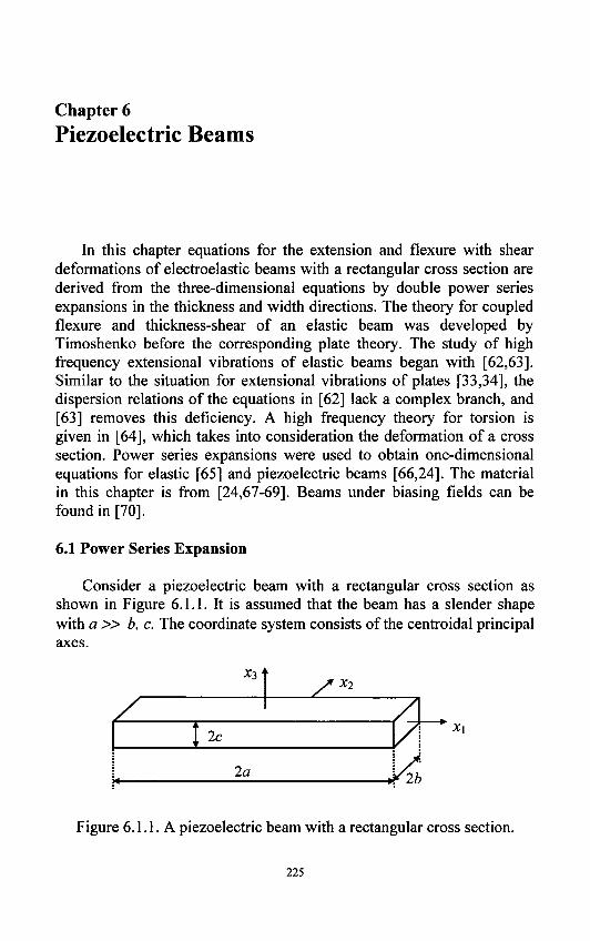
Chapter 6 Piezoelectric Beams
In this chapter equations for the extension and flexure with shear deformations of electroelastic beams with a rectangular cross section are derived from the three-dimensional equations by double power series expansions in the thickness and width directions. The theory for coupled flexure and thickness-shear of an elastic beam was developed by Timoshenko before the corresponding plate theory. The study of high frequency extensional vibrations of elastic beams began with [62,63]. Similar to the situation for extensional vibrations of plates [33,34], the dispersion relations of the equations in [62] lack a complex branch, and [63] removes this deficiency. A high frequency theory for torsion is given in [64], which takes into consideration the deformation of a cross section. Power series expansions were used to obtain one-dimensional equations for elastic [65] and piezoelectric beams [66,24]. The material in this chapter is from [24,67-69]. Beams under biasing fields can be found in [70].
6.1 Power Series Expansion
Consider a piezoelectric beam with a rectangular cross section as shown in Figure 6.1.1. It is assumed that the beam has a slender shape with a » b, c. The coordinate system consists of the centroidal principal axes.
*3
X ^L x2
2c
2a
0 2b
X\
Figure 6.1.1. A piezoelectric beam with a rectangular cross section.
225
226 Mechanics of Piezoelectric Structures
To develop a one-dimensional theory, we make the following expansions of the mechanical displacement vector and the electrostatic potential:
uJ=fjX^x"3u^"\x1,t), </>= j r ^ y ^ , / ) . (6.1.1) m,n=0 m,n=0
Then the strains and the electric field can be written as
S„ = |>2"*3"S<""">, E, = Y**ZxlE\m*\ (6.1.2) m,n=0 m,n=0
where the strains and the electric field of various orders are as follows:
$<"•"> = I[Mg-"> + u^m/n) +(m + l)(Si2u\m+hn) + SJ2ujm+l'n))
+ (n + l)(Snu^"+1) +SJ3u<»^)l (6.1.3)
£<"•"> = -$"•"> - 5I2 (m + l)^(m+1'n) - Sa in + l)^(m'n+1).
The one-dimensional equations of motion and electrostatics are obtained from the variational principle in Equation (1.2.26)
00
1lj,\ ml2j nlij +rj ~ H 2-t mnrs J ' r,s=0 (6.1.4)
A(J'n) -mDf-™ -nD\m'"-x)+D{m'n) = 0,
where the stress and the electric displacement of various orders are defined by
7 f •"> = f Tyx"x"3dA, A (6.1.5)
Df-n) = \ DrfxIdA.
A = Abe is the cross sectional area. The surface traction, surface charge and body force of various orders are
Ff*> =bm £ [ r 2 ; ( 6 ) - ( - i ) m r 2 ; ( - 6 ) K ^ 3
+ c"fb[Ty(c)-(-l)"T3j(-c)]x^dx2 + jA pf^xldA ,
Piezoelectric Beams 227
6 "C (6.1-6) + c" J [D,(c)-{-\)"D3{-c)^dx2.
-b
Bmms is a geometric quantity given by
Dmnrs ~ J^ -*2 * 3 a A .m+r „n+5
•r+m+1 s+n+1 46r+m+ics+n+1 (6.1.7) , w + r, w + s even, (r + w +1)(« + n +1)
0, else.
The one-dimensional constitutive relations take the following form: 00
y(».») _ V « (r K^'^ -e F^^h 1ij — £Jnmnrs\cijkl^kl ^kij^k h
r,s=0 (6.1.8)
D ^ = Y , B m n r s ^ i k l S ^ + S i k E ^ ) .
r,s=0
Or, with the compressed matrix notation, for p, q = 1- 6 00
i p - Z-i mnrs(-CP<l 1 eipt'i ) ' r,s=0
D^ = ±Bmnrs(eipS^+slkE^).
(6.1.9)
r,s=0
The above constitutive relations are not ready to be used. Important adjustments are necessary which will be performed later. Since piezoelectric materials are anisotropic, couplings among extension, flexure and torsion may occur due to anisotropy. For anisotropic beams, although various types of deformations may couple, usually there still exist modes which are essentially extensional or essentially flexural, which are the modes we are interested in. The essentially torsional modes will not be treated in this book.
6.2 Zero-Order Theory for Extension
First we extract a zero-order theory for extension from the general expansions.
228 Mechanics of Piezoelectric Structures
6.2.1 Equations for zero-order theory
For a zero-order theory we make the truncation
uj = uffi\xl,t) + x2uf-0)(xl,t) + x3uf-l\xi,t),
(f> = </>(m (*,, 0 + X2</>{10} (JC, , 0 + x3^°'n (xx ,t),
where u^ a nd uf» are needed to describe Poisson's effects during extension. They cannot be directly set to zero, but will be eliminated later by stress relaxations. An equation for the extensional displacement w,(0,0)
will be obtained. From Equations (6.1.3) and (6.2.1), the zero-order strains and the electric fields to be considered are
where
(0,0)
Sy
Ek
-u
~ c(0,0) - aij >
= Ei0fi)+x.
,(0,0) v(0) . 1,1 ' °22 •
rd.o)
= u™
+X340A..
C(0) _ ' °33 -
)
III0-1)
(6.2.2)
Sl°fi)=2S™=u™+u?-°\ jS(o,o)=2iS(o,o)=M(o,o)+M(o,i);
c(0,0) _ 9 o ( 0 , 0 ) _ , . (0 ,0) (1,0) ° 6 ~~ Z ° 1 2 — "2,1 i~ " l '
(6.2.3)
E^ = - ^ , E^0) = -2^ ( 2 '0 ) = 0, E™ = - ^ ( u ) = 0, (6.2.4)
E™ = -</>f», E™ = -<*(U) = 0, E™ = -2^2) = 0.
From Equation (6.1.4) the equation for extension and electrostatics are
T<-W+Ff0fi)=4pbcu[0fi), (6.2.5)
z )(i,o )_Z)(o,o )+Z)(1 ,o )=0 j ( 6 2 6 )
/ ) ( « . ! ) _ 2,(0.0)+ ^(0.1) = Q
Piezoelectric Beams 229
If there are electrodes present, some of the equations in Equation (6.2.6) need to be dropped or adjusted, as in the third section of the second chapter. The zero-order constitutive relations are obtained from Equation (6.1.9) by setting m = n = 0 and r = s = 0
A(o'o)=4M^r+44°-o)). Equation (6.2.7) should be adjusted by setting the following zero-order stresses to zero
T(0fi) = T(o,o) = ^(0.0) = ^(0,0) = ^(0,0) = 0 _ ( 6 2 8 )
In this case it is more convenient to re-derive the beam constitutive relations from the following three-dimensional constitutive relations:
Sp =SpqTq +dkp-Ek, (6.2.9)
D^d^ + slEj.
Within the approximation we are interested in, from Equation (6.2.2)
sr=v,+dkp(Er+XlEr+^D, D,=dJq+el(Ef»+X2E™+x,Ef»).
Integrating Equation (6.2.10) over the cross section of the beam, we obtain
D^=diqT^+AbcslEf0) (6.2.11)
= djt0fiU4bcelEf°\ From Equation (6.2.1 l)i, for/? = 1
AbcSffi) = suT{0fi) + 4bcdkiEi°'0), (6-2.12)
which can be inverted to give the mechanical constitutive relation for extension
*n (6.2.13)
= 4bc(cnSr)-ekiEr),
230 Mechanics of Piezoelectric Structures
where
c „ = — , 2*,= — . (6.2.14) y n
Substitution of Equation (6.2.13) into Equation (6.2.11)2 results in the following electric constitutive relations:
D^ =dnT^ +AbcsTuE^
= dn^{Sr}-dklEr) + 4bc4E?» Ml (6.2.15)
where
•Ml 'Ml
= 4bc(enSr)+ZikEri
~ „ r " i l " * l « - ) i / : \ % = f * • (6.2.16)
Mi The first-order constitutive relations needed are approximated by
or = 4Er\ or = f^r. (6.2.17) In summary, we have
T$f>+F?fi)=4pbcu\m , (6.2.18)
D$0)+DW=O,
Z)^ 0 ) -Df 0 ) +Z) ( 1 - 0 ) =0, (6.2.19)
A W ) _ Z ) ( o . o ) + j D W ) = 0 )
r/°-0) = 4bc(cuSl°'0) - eklEl°'0)), (6.2.20)
A(°'0) = 46c(2'jl51(0'0) + sikEffi)) , (6.2.21)
Aa-°)=iy£^r), A ^ — ^ ^ r , (6-2.22)
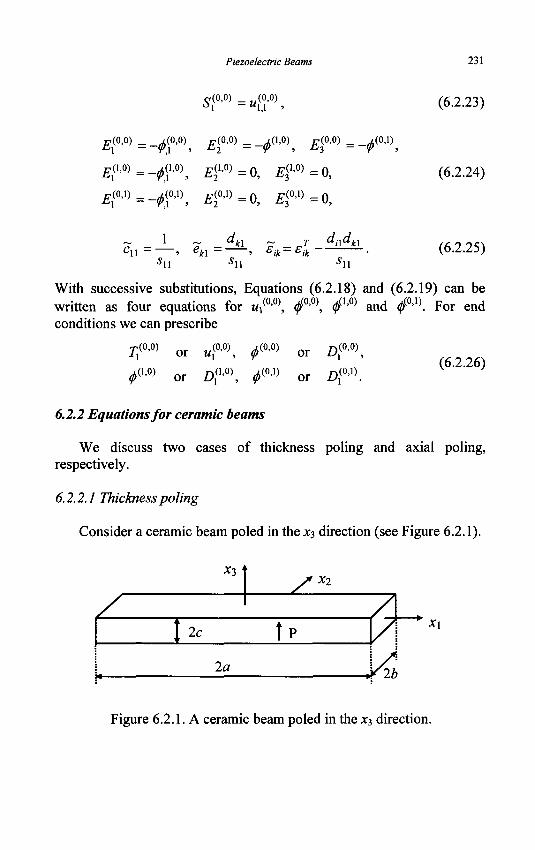
Piezoelectric Beams 231
c(0,0) _ (0,0) (6.2.23)
,(0,0)
(1,0)
(0,1)
Cll
= -*?'°\ E?fi)=-^°\ E?fi)=-= -tf-°\ ^0 )=o, £f'0)=o, = -*?», ^ w ) = 0 , £3
(0-1>=0,
_ 1 _ rftl ? _ r rf,,dM - » e i : l - > bik~bik
A(O,D
(6.2.24)
(6.2.25)
With successive substitutions, Equations (6.2.18) and (6.2.19) can be written as four equations for Wi(0'0), (jf°'°\ 0(I'O) and 0(O,1). For end conditions we can prescribe
"(0,0)
A0.O)
or u (0,0) J ( 0 , 0 )
<FW or A > (0,0)
>0.o) ^(0,1) (0,1) (6.2.26)
or A > ^ , u or A
6.2.2 Equations for ceramic beams
We discuss two cases of thickness poling and axial poling, respectively.
6.2.2.1 Thickness poling
Consider a ceramic beam poled in the x?, direction (see Figure 6.2.1).
*3
X ^L X2
2c fp Xi
2o J/2b
Figure 6.2.1. A ceramic beam poled in the x3 direction.
232 Mechanics of Piezoelectric Structures
The material matrices are given in Equation (2.4.87). Then from Equation (6.2.14) we have
~ _ 1 ~ ~ n ~ <^31 C l l = ' e l l = e2\ = 05
e31 = (6.2.27)
[**]=
rsn 0 0 A
0 en 0
33
E\\~ £W>
6 3 3 - fc33
The constitutive relations needed are
rr)=4te(c11<°>+e31^),
D^=-4bcsu^°\
(6.2.28)
(6.2.29)
(6.2.30)
£(1,0) = 4 b c „s AhQ)
A1 (0,1) _ 46c3
^ / • u \ D ^ = Z ) 3I W = 0 ,
•efo™, D™ =D™ =0.
The equations of motion and charge are
4bc(cuu^ +e^f'l)) + F^0)=4pbcul0fi)
-4bcsu^0)
+D^=0,
4b3c
3
4bc3
e^i0)+4bcsu^
0)+D^=0,
e^V -4bc(enu§0) -e33*l°A)) + D™ = 0.
(6.2.31)
(6.2.32)
(6.2.33)
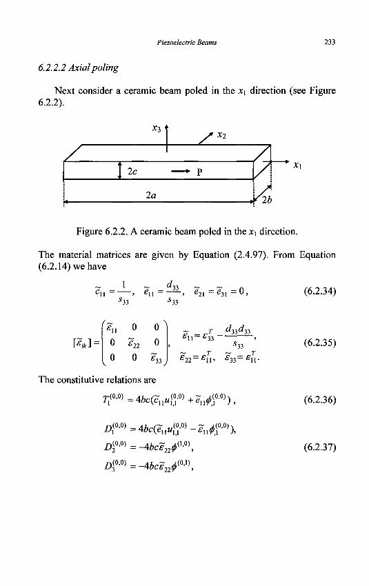
Piezoelectric Beams 233
6.2.2.2 Axial poling
Next consider a ceramic beam poled in the X\ direction (see Figure 6.2.2).
x3
z. ^L X2
2c x\
2a 2b
Figure 6.2.2. A ceramic beam poled in the jti direction.
The material matrices are given by Equation (2.4.97). From Equation (6.2.14) we have
1 c , , = • -, eH e,, =•
'33 e,i -e,, = 0, , ^21 - c31 '33 >33
(6.2.34)
[%] =
rsu 0 0 A
0 e„ 0 22
0 0 £ 33
~ _ _r ^33^33 *l l _ f c 33 '
*33 ~ _ T ~ _ 7" f 2 2 _ £ n > e33—^11-
The constitutive relations are
r/0-0>=4fe(cu«S-0)+el I tf-0)),
(6.2.35)
(6.2.36)
A ( 0 , 0 ) = ^ ^ 2 2 ^ ( 0 , 1 ) .
(6.2.37)
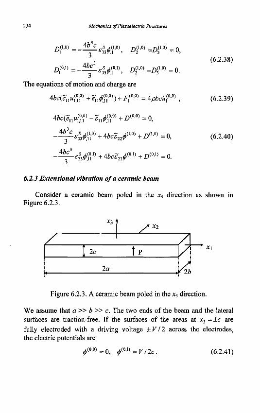
234 Mechanics of Piezoelectric Structures
(1,0) A1
n(0.D
4b3c
4bc3
• 4 # 0 4 \ ^1>0)=A(1'0)=o.
The equations of motion and charge are
4AC(eI1«gf>-giI^r+^(0-0)=0,
_ i ^ 4 ^ . » +4^2^(0-1) + # " = o.
(6.2.38)
(6.2.39)
(6.2.40)
6.2.3 Extensional vibration of a ceramic beam
Consider a ceramic beam poled in the x^ direction as shown in Figure 6.2.3.
*3
^L X2
2c fp
2a
Figure 6.2.3. A ceramic beam poled in the x$ direction.
We assume that a » b » c. The two ends of the beam and the lateral surfaces are traction-free. If the surfaces of the areas at x3 = ±c are fully electroded with a driving voltage ± V12 across the electrodes, the electric potentials are
^ • 0 ) = 0 , </P»=VI2c. (6.2.41)
Piezoelectric Beams 235
From Equations (6.2.32) and (6.2.29) we have the following boundary value problem:
cuu^ = pui°'°\ -a<xx<a, U 1 (6.2.42)
7i(0'0) =Abc{cuu\Y) + e 3 / ° ' 1 ) ) = 0, xx=±a. Equation (6.2.42) shows that the applied voltage effectively acts like two extensional end forces on the beam. For free vibrations, V = 0 and the electrodes are shorted. We look for free vibration solutions in the form
u{m (*i, 0 = w, (*!) exp(HHf). (6.2.43)
Then the eigenvalue problem is
u,,, +p<y2snM, =0, - a< j c , <a, i.ii ^ ii i ' i (6.2.44)
wt j = 0 , Xj = ± a .
The solution of co= 0 and w = constant represents a rigid body mode. For the rest of the modes we try u = sin&C]. Then, from Equation (6.2.44)i,
k = co.yjpsu . To satisfy Equation (6.2.44)2 we must have
cosAa = 0, => &(n)a = — , n = 1,3,5, •••, (6.2.45)
or
/w n a = —-, fl)(n) = = = , /i = l,3,5,--. (6.2.46) 2 2aV/»ii
Similarly, by considering w = cosfcci, the following frequencies can be determined:
co{n) = ™ , » = 2,4,6,- . (6.2.47) 2aylpsu
The frequencies in Equations (6.2.46) and (6.2.47) are integral multiples of a>m and are called harmonics. o(1) is called the fundamental and the rest are called the overtones. These results are the same as those in [9].
6.3 First-Order Theory
Next we truncate the general expansions to obtain a first-order theory for coupled extension, flexure, thickness-shear and width-shear [24].
236 Mechanics of Piezoelectric Structures
6.3.1 Coupled extension, flexure and shear
For a first-order theory, to include all first-order strains, we make the following truncations:
J J *• J J J *• J *• J J J J / r -j -I \
where u2'0), u(
2'0), u\0,1) and uf'1^ are needed to describe Poisson's
effects accompanying extension and flexure. They cannot be directly set to zero, but will be eliminated later by stress relaxations. Equations for
the extensional displacement uf'^ , flexural displacements uf'0) and
uf'0) , and thickness-shear and width-shear displacements w,(1'0) and
wj0'1* will be obtained. From Equations (6.1.3) and (6.3.1), the strains and electric fields are
c ~ e(°,0) c,(i,0) o,(0,i)
Ek^E?»+x2Er+x,Er,
where the zero-order strains are given by
(6.3.2)
£(0,0)
£(0,0)
£(0,0)
£(0,0)
- u{0'0)
_ 9 c(0,0) - Z l 323
= 2 < 0 )
= 2Sl°2'0)
the first-order strains, <
c(0) _ °22 ~
- w ( 0 '0 )
_ " 3 , 1 - u{m
,.0.0) c(0) "2 ' °33
+ «3°'°).
+ « , ( , U ) ,
+ Wl(1'0).
= «i°J ) ,
anly the following expressions are
sr = s™ =
"1,1 '
'"iT-
(6.3.3)
needed:
(6.3
(6.3
•4)
.5)
The rest of the first-order strains will be eliminated by stress relaxations. The relevant electric fields are
Piezoelectric Beams 237
E?fi)=-j$fi\ E^0)=-2^2fi)=0, E?fi)=-j™=0, (6.3.6)
£<<>•» = -<t>f», E<?-1) = - ^ = 0, E?» = -2^ ( 0 '2 ) = 0.
We keep the equations of motion corresponding to the extension Wi(0'0), flexure M2(°'0) and W3(0'0), and shear deformations wi(1'0) and «i(0,1):
T^UF^=pAuffi\
TQf+F}0-0)=Mul°fi\ (6-3.7)
T^-T^+F^^pAr2u^\
Tw)-T(0fi)+Fm=pAr2iimt
where
A = Abc, r2=c2/3, r2=b2/3. (6.3.8)
ri and r^ are the radii of gyration of the cross section about the Xj and *3 axes. For electrostatics we keep the equations for (/f0'°\ 0 , 0(O1)
A(,r+0(o-o)=o, z)(i>o)_jD(o>o)+jD(i,o)=0j ( 6 _ 3 9 )
z?(o,i)_Z)(o,o)+D(o,i) ;=0
For the zero-order mechanical constitutive relations we have, from Equation (6.1.8)1, for m = n = 0,
7 f 0 ) = 4 ^ c „ S ? - 0 > - ^ ° > ) . (6.3.10)
Equation (6.3.10) should be adjusted by setting the following zero-order contour stresses to zero [65]
r2(0 '0)=:r3 (0-0)=r4
(0-0)=o, (6.3.11)
which permits the free development of the corresponding zero-order
contour strains. Equation (6.3.11) will be used to eliminate Sf'0^, S^0'0^
and S?fi) from Equation (6.3.10). In view of the conditions in Equation (6.3.11), we now introduce an index convention which will be of
238 Mechanics of Piezoelectric Structures
(6.3.12)
considerable use to us in the sequel. The convention is that we let the subscripts oc, /3 take the values 1, 5, 6 and A, fi, v take the remaining values 2, 3, 4. Then Equation (6.3.10) can be written as
nm=4bc(Ca^p+Ca^r -e^rh Tr^bc(cx^r+cXfJsr-eaEr).
With this convention Equation (6.3.11) can be written as
7 f ' 0 ) = 0 , (6.3.13)
which implies, with Equation (6.3.12)2, that
AbcS^ = -4bccic0Sf» + 4bccZelMEW, (6.3.14)
where c~x is the matrix inverse of cX/J:
cZC^=S».v (6-3-15) Substitution of Equation (6.3.14) into Equation (6.3.12)i yields the relaxed zero-order mechanical constitutive relations
^ • 0 ) = 4 M ^ 4 0 ' 0 ) - ^ ^ ( 0 ' 0 ) ) , (6-3.16) where
Cap =Cafi ~CaXCXftCnP> eia = eia ~ eifiCfUcA.a- (6.3.17)
For the zero-order electric constitutive relations we begin with Equation (6.1.8)2 for m = n = 0
= 4bcielaSr^aSr+8lkED.
Substituting Equation (6.3.14) into Equation (6.3.18), we obtain
Dr^Abcie^Us^r), (6.3.19)
where
£ik=£ik+eac~xlek,f (6.3.20)
Piezoelectric Beams 239
If two shear correction factors K2 and K3 are introduced by the replacement of the following thickness-shear and width-shear strains in the strain energy:
4° ' 0 ) -* *2£l(2'0). SU0) -+ "IS™' (6-3-21)
the zero-order constitutive relations will be modified into
Tr)=*bc{d'apSp-~e'iaEr)),
Dr^tbcielpSp+e^r). (6.3.22)
Equation (6.3.22) depends on the strains S\m, S?fi) and Sf'0), which are related to the extensional, flexural and shear displacements.
For the first-order mechanical constitutive relations from Equation (6.1.8)1 we obtain, by setting m = 1 and n = 0,
T™ ~<P„SW-e¥E?*>). (6.3.23)
Equation (6.3.23) should be adjusted by setting the following first-order beam stresses to zero:
7f°> = T?fi) = 7f0) = 7f0) = 7f0) = 0, (6.3.24)
which permits the free development of the corresponding first-order
strains. Equation (6.3.24) can be used to eliminate S$fi), S$fi) S%'0),
S^l'0) and S£'0) from Equation (6.3.23). In this case we re-derive the beam constitutive relations from the following three-dimensional constitutive relations:
Sn -snaTa
+dknEk, (6.3.25)
D^d^ + e'yEj.
Within the approximation we are interested in, from Equation (6.3.2)
S™+x2S™+X3S™
= spqTq +dkp(E?» + x2E™ +x3Ei°»), (6.3.26)
Dl^dlqTq+eT
yiEf^+x2E^+x3E^).
240 Mechanics of Piezoelectric Structures
Integrating the product of Equation (6.3.26) with x2 over the cross section of the beam, we obtain
- v r ( i -Q) • 4 b c d E-0.0)
D r = d i j r + ^ £ T E r
(6.3.27)
From Equation (6.3.27)i, forp = 1
4bcsr=snTr^dk:Er, (6.3.28) n l 1 x 1 s\
which can be inverted to give
r f t o ) = J . 4 ^ £ ( W )_ a.0))
sn 3
4b3c (6.3.29)
(crf^^D-Substitution of Equation (6.3.29) into Equation (6.3.27)2 results in the electric constitutive relation
A ( ,-0)=M°-0)+^W )
Su 5 5
= 463c dn a o ) 46jc r _^Aa_)E(.i,o) 3 1 ?y \ IK ' K
The above first-order constitutive relation is for flexure in the x2 direction. Similarly, for flexure in the JC3 direction,
(6.3.30)
Piezoelectric Beams 241
rr ~(cusr-enEn 3 (6.3.31)
In Equations (6.3.29) through (6.3.31) only the shear strains 5,(1'0) and
S^ appear, which depend on the shear displacements. In summary, we have obtained
Ttff+F{W=4pbcut0fi\
T$P+F^=4pbcuffi\
T$P+F?fi)=4pbcu¥fi\ (6.3.32)
T™ -T™ +F™ =±pb3cu?fi\
T$? - 4 ° ' 0 ) +^1(0'1) = -pbc3u™,
D(o,o)+Z)(o,o)=0;
D$0)-Dl0fi)+DQfi)=0, (6.3.33)
T^fi) = *bc{c'apsp -e'iaEr]), a,fi = 1,5,6,
Tr}=^(cusr-eklEri
(6.3.34)
(6.3.35)
242 Mechanics of Piezoelectric Structures
?(0,0) _ „(0,0) > 1 - " 1 , 1 '
C i i = • , ckx - , 0jk- aik
(6.3.36)
6.3.37)
^• 0 )=M l(7, ^ - " f f , (6.3.38)
£(o,o) = _^(o,o)5 £(o,o) = _^(i,o)) £(o,o) = _^(o,D5
^ ' ^ f , £2°'0)=0, E™=0, (6.3.39)
Ca/3 =Cap ~CaXCXfiCfifi' eia ~eia ~einC^CXa>
£ik = £tk + eacZeku» «> /? = ^5,6, A,fi,v = 2,3,4, (6.3.40)
With successive substitutions, Equations (6.3.32) and (6.3.33) can be written as eight equations for Ml
(0'0), M2(0'0), W3
(0,0\ u{m, Ul™\ f'°\ f'0)
and 0(O1). For end conditions we can prescribe
7;(0'0) or Ml(0'0), 7f-0) or u?'°\ 7f0 ) or uf'°\
7f0) or Ml(1'0), T™ or u™, (6.3.41)
(o,o) o r A(o,o)j ^(i,o) o r (1,0) (o,i) o r A(o,i)_
6.3.2 Reduction to classical flexure
For the theory of elementary flexure without shear deformations, we set the rotatory inertia terms in Equations (6.3.32)45 to zero:
Piezoelectric Beams 243
r (Y)_ r (o .o)+ Fd,o)= 0
' (6.3.42) r ( 0 , l ) r ( 0 , 0 ) F ( 0 , l ) _ n
V
111,1 Y31 + M ~ U>
which can be used to solve for r2i(0'0) and 73i(0'0). Substitute the resulting
expressions into Equations (6.3.32)2,3
r(1.0> + F d . 0 ) + F ( 0 , 0 ) = ^ ( 0 , 0 ) ii.li 1,1 2 A- 2 (6.3.43)
which are the equations for elementary flexure. We also need to set the zero-order shear strains to zero
5f0)=i4°-0)+«1(1'0)=0,
so that the first-order flexural strains can be represented by .(0,0 *3,11
T^ =Abc(c'uS[ofi) -e'nE?-0)),
D^=4bc(e'nSl0fi)+£lkEl0>0)),
TT(O.O) _ T ( l , 0 ) , 1^(1,0) i 2 1 -• '11,1 + Y 1 >
r ( 0 , 0 ) _ r ( 0 , l ) - (0 ,1) "*31 - • '11 ,1 i " - r l >
(6.3.44)
51(1-0)=-4°f?), S f ' ^ - i ^ j 0 . (6.3.45)
The equations for the classical theory are
ri(o,o)+Fi(o,o)=4p^(o,o)5
T<?f + F2(0'0) = 4pbcii?<0), (6.3.46)
T$f+FW=4pbcul0fi\
/ ) ( ' . " )_ ^(0.0 + / j ( i . o ) = 0 j ( 6 _3_ 4 7 )
Z)(o.i)_Z)(o,o)+jD(o,i)=0)
(6.3.48)
(6.3.49)
244 Mechanics of Piezoelectric Structures
Dr~ensr+z*EP),
(6.3.50)
(6.3.51)
Sf0) = u$°\ Sf°> = -«£•?>, S™ = -ui°», (6.3.52)
£(°-°) = -^f°>, £ f °> = -^0.0) j ^(o.o) = _^(o,i)
^•°)=-^j1-°) , i ^ ^ O , ^ ° ) = 0 , (6.3.53)
E ^ = - ^ \ £ M = 0 j £(o.i) = 0 .
With successive substitutions, Equations (6.3.46) and (6.3.47) can be written as six equations for Wl
(0'0), uffi\ uffi), f'°\ ffi) and f». For end conditions we can prescribe
r / ° - 0 ) or Wl(0-0), r6
(0-0) or u\' \ T$ '° or u^' \ r,(I-0) or u%f\ T™ or uff, (6.3.54) ^(0,0) o r A ( 0 , 0 ) ; ^(1.0) ^ A ( l , 0 ) 5 ^(0,1) Q r £,(0,1) _
6.5.5 Thickness-shear approximation
Consider the beam in Figure 6.3.1. The material of the beam is of general anisotropy.
6.3.3.1 Equations for coupled flexure and thickness-shear
We study motions dominated by coupled thickness-shear w,(01) and
flexure uf'0^. The major mechanical resultants are the shear force T^
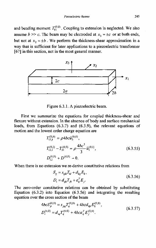
Piezoelectric Beams 245
and bending moment T^'X). Coupling to extension is neglected. We also assume b » c. The beam may be electroded at x3 = ±c or at both ends, but not at x2=±b . We perform the thickness-shear approximation in a way that is sufficient for later applications to a piezoelectric transformer [67] in this section, not in the most general manner.
*3
2c
2a
Z. X2
71 r2b
Xi
Figure 6.3.1. A piezoelectric beam.
First we summarize the equations for coupled thickness-shear and flexure without extension. In the absence of body and surface mechanical loads, from Equations (6.3.7) and (6.3.9), the relevant equations of motion and the lowest order charge equation are
r (0 ,0) ^ 13,1
T(0U Ml,l "
n(0.0) •^1,1
xtensic s„ A
= pAbcuf'°\
-rr=P4bf> + Z)(0-0)=0.
MI we re-derive c(
= sijld^kl +"kijEjc>
= dijkTjk+slEj.
:;(0,1) (6.3.55)
(6.3.56)
The zero-order constitutive relations can be obtained by substituting Equation (6.3.2) into Equation (6.3.56) and integrating the resulting equation over the cross section of the beam
(6.3.57) AbcSf0) = spqT^+AbcdkpEl
D (0,0) = J r (0 ,0)
uiq1q + AbcsljEj (0,0)
246 Mechanics of Piezoelectric Structures
We keep the dominating shear force 7,5(0,0) and make the following stress
relaxation:
7 f 0 ) = 0 , ? = 1,2,3,4,6. (6.3.58)
Then, for/? = 5, Equation (6.3.57) becomes
AbcSf* =sssT™U*bcdk5E?m, (6.3.59)
D^=dl5T^+4bc^Effi\ K }
Equation (6.3.59) can be inverted as
T?» =^{K2S?» -Kdk5E?»\ 555 (6.3.60)
D\W =Abc&KS?V +euEfn\
where rc(= KX) is a shear correction factor, and
~ T "i5"j5 ttil aw £u=£y — • (6.3.61)
Integrating the product of Equation (6.3.56)i with x3 over the cross section, we obtain
^fs™ = v r +^fdkpEr- (6-3.62)
For flexure, j / 0 ' ^ is the dominating resultant. We make the following stress relaxation:
T f ' ^ 0 , 9 = 2,3,4,5,6. (6.3.63)
Then, for/? = 1, Equation (6.3.62) becomes
^Sr='nli°»+^fdHEr, (6-3-64)
which can be inverted as
r(o,D = i*£l(5(o,i) -duE{°»). (6.3.65) 3*ii
Piezoelectric Beams 247
The relevant strains and electric fields are c(0,0) _ (0,0) (0,1) o(0,l) _ (0,1) ^ 5 - M3,l + U\ > ^1 ~ Ml,l '
With successive substitutions, Equation (6.3.55) can be written as three equations for w3
(0'0) and well as the electrostatic potential 0(O'O)
*55
—(-W + ^ n ^ 1 ) ) - ^ - [ ^ 2 « ) +«,(°-,)) c2555 (6.3.67)
+ «/15^0-0)+M/35^0 '1)] = piiI(0-,),
^ ^ f ) +«™)-*n*<r - ^ r +7rD(0,0) =0' s55 Abe
where Ef'^ has been dropped in view of the ceramic piezoelectric transformer we are going to analyze later using these equations. The expression for D3
(00) in Equation (6.3.60)3 is not used in Equation (6.3.67), but it is useful for determining the electric charge on an electrode when a beam is electroded at JC3 = ±c. For a beam electroded at JC3 = ±c, 0(O'O) is no more than a function of time and Equation (6.3.67)3 is not needed. For an unelectroded beam, Equation (6.3.67)3 is needed to determine 0(O'O).
6.3.3.2 Thickness-shear approximation
Next we study the thickness-shear approximation. When the beam is vibrating essentially at thickness-shear modes, the coupling to flexural motion is weak and can be eliminated by the thickness-shear approximation. For this simplification we proceed as follows. Consider the following simple wave solution:
L(0,0) (0,1) .(0.0) -(0,1)1
t"3 ' Ml ' * ; * > (6.3.68) = {A, B, C, £>}exp[i(£i + A*)].
248 Mechanics of Piezoelectric Structures
Substituting Equation (6.3.68) into (6.3.67)i yields the following relation:
— [ K 2 (-£2A + i£B) - Kdl5£2C + Kd35i£D] = -pco2A. (6.3.69)
For long waves, the wave number % is small. Hence we drop the quadratic terms of E, in Equation (6.3.69). Furthermore, since we consider vibrations at frequencies very close to the lowest thickness-shear frequency ax^of an infinite beam, we set of ~ a}„ in Equation (6.3.69). We then obtain the following approximation of Equation (6.3.69):
A = 1 (K2i@ + Kd35i$D), (6.3.70)
which is equivalent to the following differential relation:
«f°> = ^ 2 < ] ) + xd^r). (6-3.71)
Substituting Equation (6.3.71) into Equation (6.3.67)2, we obtain the following equation for long thickness-shear waves:
,2 1 jyW) 3 g „(<U)
~TU,\\ "~2 U\ Su C S55
+ ^ 1 L ^ ) _ 3^.^(0.1) _ M i ^ ( o , o ) =pfi(o.D j
su c s55 c s55
(6.3.72)
where
1 _ 1 , 3y4 d*n _ du 3K3d35 — = + 2 2 2 ' - ^ ~ + 2 2 2 " (6.3.73)
For the electric potential we drop the second derivative term of M 3( ° ' 0 ) in
Equation (6.3.67)3, which is small for long waves, and obtain
^ u ™ -ent?{0) -e13tf» + — Z)(0'0) =0. (6.3.74) Sec ^rOC
Thus we have eliminated the flexural displacement «3°'0) and obtained two equations, Equations (6.3.72) and (6.3.74), for the shear displacement uf'1^ and the electric potential <ff°'°\ Under the above thickness-shear approximation, the resultants are approximated by dropping second derivative terms
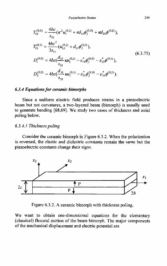
Piezoelectric Beams 249
7,(0,0) -M3
n (0,1)
Abe
4bc3
3s,,
(K2U^+Kdl5<t>?fi)+KCti5^),
(U\y>+dufr) (0,1) >
A(°-°) =4bc&-KU™ -slj?fi) - 4 * ( ( M ) ) , (6.3.75)
5 55
z)(°-°) = ^ ( ^ L / a ^ - 4 ^ ° - 0 ) -4* ( 0 > 1 ) ) . '55
6.J.4 Equations for ceramic bimorphs
Since a uniform electric field produces strains in a piezoelectric beam but not curvatures, a two-layered beam (bimorph) is usually used to generate bending [68,69]. We study two cases of thickness and axial poling below.
6.3.4.1 Thickness poling
Consider the ceramic bimorph in Figure 6.3.2. When the polarization is reversed, the elastic and dielectric constants remain the same but the piezoelectric constants change their signs.
*3
2c
X2
^L TF 1
Xi
— •
2b
Figure 6.3.2. A ceramic bimorph with thickness poling.
We want to obtain one-dimensional equations for the elementary (classical) flexural motion of the beam bimorph. The major components of the mechanical displacement and electric potential are
250 Mechanics of Piezoelectric Structures
UX(*!,X2,X3,t) = -X2uff](Xj,0 - *3l4j ,0)(*,,t),
u2 (x, ,x2,x3,t) = ui°'0) (x,, t), (6.3.76)
W3 (X\, JC2 J 3 J • ) = M3 ' (*i j 0»
where the thickness- and width-stretch displacements u2'0) and uf,l)
are not explicitly given, but they are not zero. ^(0'0) is responsible for
the axial electric field in the x\ direction, ^ (10) and ^°'l) are related to
the lateral electric fields in the x2 and JC3 directions. Equation (6.3.76)
implies S, = x2S[x'0) + x3S^,l) and the following beam strains and
electric fields:
S,™ =-«£?>, Si0" =-"%?, (6-3.77)
E{W=-4f-°\ Ef'0)=-^°\ £f0)=-^°.». (6.3.78)
5'1(1'0) and 5'1
(0'1) represent bending curvatures in the x2 and JC3 directions. We are only interested in the zero-order electric field. The equations of flexure and electrostatics are
T™+Fft0)+F™=4pbcuQfi\ ' (6.3.79)
Ttf$ + + ^3(°'0) = */*"*¥ •0),
Z )(o,o ) + Z )(o,o)= 0 ; ( 6 3 8 0 )
where the equations corresponding to ^(1'0) and ^ (01) are not included. 7,
1(110) and T^ are the bending moments in the x2 and ;e3 directions.
For long and thin beams, since T22 = T2z = 0 at x2 = ±b and 733 = T32 = 0 at X3 = ±c, these stress components are also very small inside the beam and are approximately zero everywhere. When the beam is not in pure bending, there are shear stresses Tu and Txi related to bending which are responsible for the shear resultants ri2
00) and 7,13°'0). For ceramics, shear
and extension are not coupled. Therefore, in calculating the bending strains, the only stress component that needs to be considered is Tu.
Piezoelectric Beams 251
^.(1,0) = f, Tux2dA=\ —(Sx -dklEk)x2dA JA JA .v..
With the compact notation, Tx=sxx(Sx -dkXEk) and the bending
moment in the x2 direction is
_i JA " " JA s,
2 3 (6-3.81) = 50.0)f ^ _ £ ( ° . ° ) f x ^ L d 4 = i*£ 5 0,o) >
•M sxx >* sxx 3sxx
which is not coupled to the electric field considered as expected. Similarly, the bending moment in the x3 direction can be written as
T™ = f Tnx3dA=\ —(Sx -dkXEk)x3dA JA JA c.. •A Su
= 5(o.i)f *LdA-E?fi~>\ x3^dA (6.3.82) JA M.. JA v.. JA sn
JA sxx
Abe1 (0>i) 2c2bd3X F ( 0 0 )
3 s n o n
which is electrically coupled to ^(01) as expected. The electric
constitutive relation of interest is found to be
Z)f0) = I D3dA= I (d3pTp+e3JEj)dA
= £ (d3xTx+e3jE^dA
= \A [ < W ( S i -dkXEk) + s3jEj]dA ( 6-3-8 3 )
2c2bd, ^sr+*bcZ*E, (0,0)
£ >
where S = x2iS,,(10) + x3Sx
0'^ has been used and
£ik=sJk-dndkl/sxx. (6.3.84) Within the classical theory, the transverse shearing forces in the beam are related to bending moments by
T(0,0) _ r ( l ,0 ) c-0,0) •M2 — -Mil ~l~-rl '
(6.3.85) r(0,0) _ r (0 , l ) F(0,\) V ' -M3 — -* 11.1 1
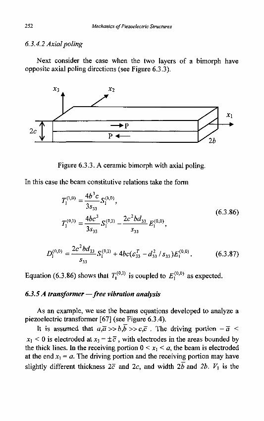
252 Mechanics of Piezoelectric Structures
6.3.4.2 Axial poling
Next consider the case when the two layers of a bimorph have opposite axial poling directions (see Figure 6.3.3).
2c J
*3 X2
— •
2b
Figure 6.3.3. A ceramic bimorph with axial poling.
In this case the beam constitutive relations take the form
4b3c j(l,0)
j(0,l)
3s - ^ • 0 ) ,
33
4fo Q(O,I) 2c bd33 p(o,o) 3s
(6.3.86)
33 5 33
Dl0fi) = 2c2bd-33 o(0,l)
S?»+Abc{ei3-di3lsi3)E, (0,0) (6.3.87)
'33
Equation (6.3.86) shows that r/0'1' is coupled to E,(0'0) as expected.
6.3.5 A transformer—free vibration analysis
As an example, we use the beams equations developed to analyze a piezoelectric transformer [67] (see Figure 6.3.4).
It is assumed that a,a »b,b »c,c . The driving portion -a <
x\ < 0 is electroded at x^ = ±c , with electrodes in the areas bounded by the thick lines. In the receiving portion 0 < x\< a, the beam is electroded at the end *i = a. The driving portion and the receiving portion may have
slightly different thickness 2c and 2c, and width 2b and 2b. V\ is the
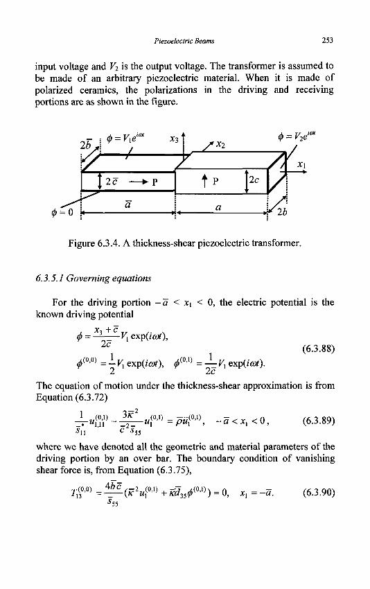
Piezoelectric Beams 253
input voltage and V2 is the output voltage. The transformer is assumed to be made of an arbitrary piezoelectric material. When it is made of polarized ceramics, the polarizations in the driving and receiving portions are as shown in the figure.
0 = V2e"
Figure 6.3.4. A thickness-shear piezoelectric transformer.
6.3.5.1 Governing equations
For the driving portion -a < x\ < 0, the electric potential is the known driving potential
x3 +c f= VyexpQa*),
0<°-°> = 1 F , exp(icot), 0(o'1) =-^=Vi exp(ia*). 2 2c
(6.3.88)
The equation of motion under the thickness-shear approximation is from Equation (6.3.72)
1 „(<U) 3*~ ,.(0.1) _ niiW) 3 T w l 11 ~ _ 2 _ u\ ~ Pu\ > - M ^ * I S,, ' C S
a < xx < 0 , (6.3.89) Ml w °55
where we have denoted all the geometric and material parameters of the driving portion by an over bar. The boundary condition of vanishing shear force is, from Equation (6.3.75),
r(o.o) = i 5 £ ( j f 2 (o,i) + ^ ^ ( 0 . 1 ) ) = o, Xl= -a. (6.3.90) *55
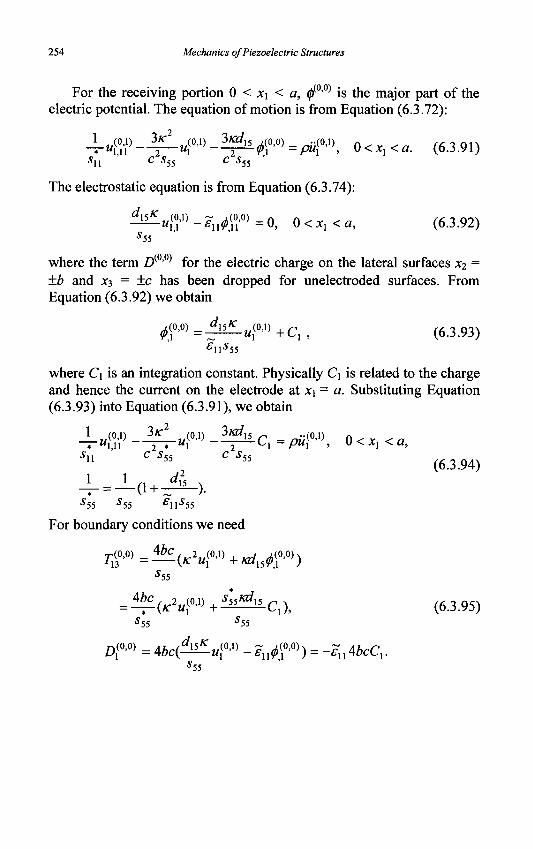
254 Mechanics of Piezoelectric Structures
For the receiving portion 0 < x\ < a, 0(OO) is the major part of the electric potential. The equation of motion is from Equation (6.3.72):
4-H&" - ^ « , ( ( U ) - ^ 4 ° ' 0 ) = p%°-l\ 0< xx < a. (6.3.91) 11 55 55
The electrostatic equation is from Equation (6.3.74):
— " f t 0 - *n*(ii,0) =0, 0 < xx < a, (6.3.92)
where the term Z)(00) for the electric charge on the lateral surfaces x2 = ±b and X3 = ±c has been dropped for unelectroded surfaces. From Equation (6.3.92) we obtain
^ ( o . o ) = ^ £ . (0 , i ) + c ( 6 3 9 3 )
where C\ is an integration constant. Physically C\ is related to the charge and hence the current on the electrode at x\ = a. Substituting Equation (6.3.93) into Equation (6.3.91), we obtain
1 (o,i) 3/r (on JKM] ~^rMi,n 2 sn c s
(o;i) __i!L_„(o,i) -""*is n _ ^,"(0,1) 1,11 2 »
11 C 5 55
u\i\ —T^~u\"' —TALQ\ = M ' ° < *i < a> (6.3.94)
4,_L 0 +JSL.) .
For boundary conditions we need
7;(o.o) = 46£(/l.2I/(o,i)+K/i^(o.o))
= ^£ (^M(o, i) + 4 ^ H C l ) , (6.3.95)
*55
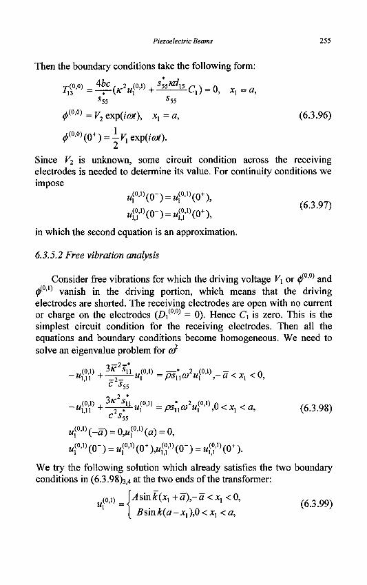
Piezoelectric Beams 255
Then the boundary conditions take the following form:
40.0) = i?£(^Ml«U> +^A-CX) = 0, xx=a,
^(0'0) = V2 exp(zfttf), JC, = a, (6.3.96)
^°-°)(0+) = iF1expO^).
Since F2 is unknown, some circuit condition across the receiving electrodes is needed to determine its value. For continuity conditions we impose
«{0-1)(0-) = u1(0'1)(0+),
(6.3.97) «S",)(o-)=i«S-,)(o+),
in which the second equation is an approximation.
6.3.5.2 Free vibration analysis
Consider free vibrations for which the driving voltage V\ or 0(O'O) and (f'1^ vanish in the driving portion, which means that the driving electrodes are shorted. The receiving electrodes are open with no current or charge on the electrodes (A(0'0) = 0). Hence C\ is zero. This is the simplest circuit condition for the receiving electrodes. Then all the equations and boundary conditions become homogeneous. We need to solve an eigenvalue problem for GJ2
_tt(o.i) + ^ L „ 1 ^ =psWu\»'x\-a <xx <0, c s55
_„(o.i) + ^ i M i W ) = ^ y w . O <xx<a, (6.3.98) c s55
ur\-a) = 0,ur\a) = 0,
«ri)(o-)=»1(o>i)(o+),<i)(o-)=<i)(o+).
We try the following solution which already satisfies the two boundary conditions in (6.3.98)34 at the two ends of the transformer:
M(o,D = Usmk(Xl + a)-a<xl<0, ^ ^
I 5sin k(a - xx ),0 < xx < a,
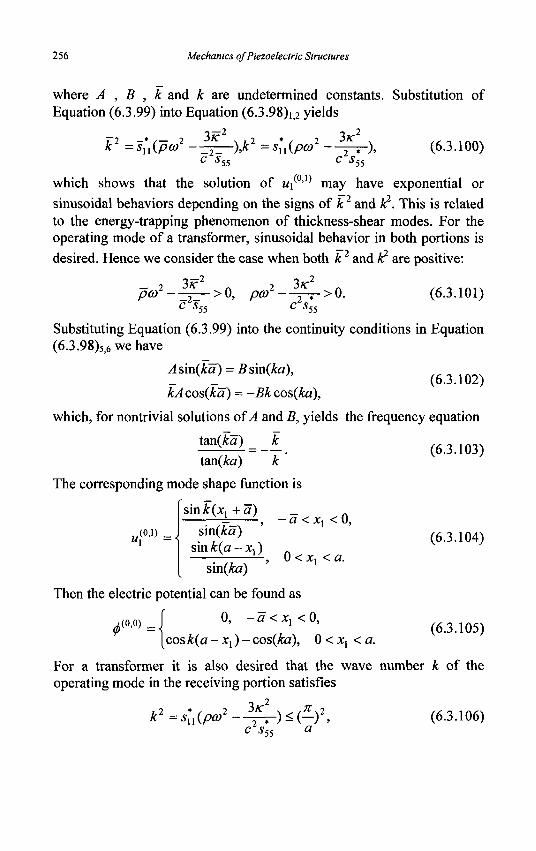
256 Mechanics of Piezoelectric Structures
where A , B , k and k are undetermined constants. Substitution of Equation (6.3.99) into Equation (6.3.98)12 yields
T~2 —• /— 2 3/C \ I 2 * r 2
k = su(pco -—yZ—)>k = su(P<» 3K
c2s 55 c s - ) , (6.3.100) 55
which shows that the solution of w/0'^ may have exponential or
sinusoidal behaviors depending on the signs of k2 and k2. This is related to the energy-trapping phenomenon of thickness-shear modes. For the operating mode of a transformer, sinusoidal behavior in both portions is
desired. Hence we consider the case when both k2 and k2 are positive:
- 2 I* A 2 pco - _2_ > 0, pa> c s
3K2
.2 * >0.
55 c s (6.3.101)
55
Substituting Equation (6.3.99) into the continuity conditions in Equation (6.3.98)5>6wehave
Asin(ka) = Bs'm(ka),
kAcos(ka) = -Bkcos(ka),
which, for nontrivial solutions of A and B, yields the frequency equation
tan(&a) _ k
tan(ka) k
The corresponding mode shape function is
sinA:^ +a)
(6.3.102)
(6.3.103)
«< W ) = sm(ka) sin k(a -xx)
- a < JC, < 0,
0 < xx <a.
(6.3.104)
sm(ka)
Then the electric potential can be found as
t(o.o) _ J 0» -a<x{<0 f I cosk{a-xx)-cos{ka), 0<xx <a.
(6.3.105)
For a transformer it is also desired that the wave number k of the operating mode in the receiving portion satisfies
k2 =s*u(pa>2 3K 2T-)±{-)\
c s 55 a (6.3.106)
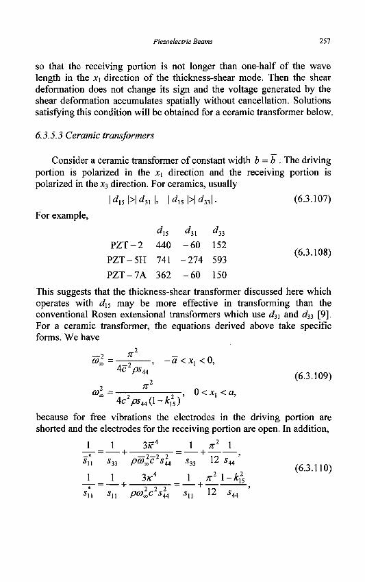
Piezoelectric Beams 257
so that the receiving portion is not longer than one-half of the wave length in the x\ direction of the thickness-shear mode. Then the shear deformation does not change its sign and the voltage generated by the shear deformation accumulates spatially without cancellation. Solutions satisfying this condition will be obtained for a ceramic transformer below.
6.3.5.3 Ceramic transformers
Consider a ceramic transformer of constant width b = b . The driving portion is polarized in the JCI direction and the receiving portion is polarized in the x^ direction. For ceramics, usually
(6.3.107)
(6.3.108)
This suggests that the thickness-shear transformer discussed here which operates with d\5 may be more effective in transforming than the conventional Rosen extensional transformers which use diX and d^ [9]. For a ceramic transformer, the equations derived above take specific forms. We have
- 2 * ' -
®«>=—; , -a<xx<0,
4c ps44
a<° = 771 7—TTT' ° < *i < a '
For example,
1 dXi |>| d3l
PZT-2 PZT-5H PZT-7A
|, \dl5\>\d33\.
"15 "31 "33
440 - 6 0 152
741 -274 593
362 - 6 0 150
(6.3.109)
4 c > 4 4 ( l - ^ 5 )
because for free vibrations the electrodes in the driving portion are shorted and the electrodes for the receiving portion are open. In addition,
_L = J_ 3/c4 _ 1 ^__\_ sn £33 pa>xc 5 4 4 S33 12 5 4 4
(6.3.110) _L = J_ 3y4 _ 1 n1 \-k?5
* ~ + 2 2 2 _ "** n ' SU S\i P«><oC 5 4 4 SU 12 Su
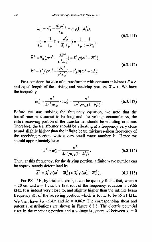
258 Mechanics of Piezoelectric Structures
£u - £n - £u(l - kl5),
(6.3.111)
\-ki '55 J 44 C 11 J 44 J 4 4 l ^15
7"2 —» / 2 3K" \ —* / 2 2 \
k =su(pa) -—2 ) = sup(o) -6>K),
• s 2 3 / f . » 2 2% s n ( / ™ — 2 - ? - ) = *iiP(<y -<» . ) .
c s,
(6.3.112)
'55
First consider the case of a transformer with constant thickness c - c and equal length of the driving and receiving portions a-a. We have the inequality
®i = — ? «& = A2 n
n , 2 • (6.3.113)
Before we start solving the frequency equation, we note that the transformer is assumed to be long and, for voltage accumulation, the entire receiving portion of the transformer should be vibrating in phase. Therefore, the transformer should be vibrating at a frequency very close to and slightly higher than the infinite beam thickness-shear frequency of the receiving portion, with a very small wave number k. Hence we should approximately have
4c> 4 4 ( l -4) Then, at this frequency, for the driving portion, a finite wave number can be approximately determined by
P =s;iP(o)2 -al)«fxxp(a>l -ml). (6.3.115)
For PZT-5H, by trial and error, it can be quickly found that, when a = 20 cm and c = 1 cm, the first root of the frequency equation is 59.66 kHz. It is indeed very close to, and slightly higher than the infinite beam frequency GL, of the receiving portion, which is found to be 59.31 kHz. We then have ka = 5.4TT and ka = 0.86TT. The corresponding shear and potential distributions are shown in Figure 6.3.5. The electric potential rises in the receiving portion and a voltage is generated between x\ = 0
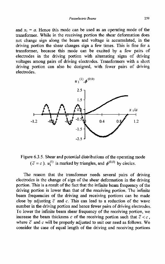
Piezoelectric Beams 259
and x\ = a. Hence this mode can be used as an operating mode of the transformer. While in the receiving portion the shear deformation does not change sign along the beam and voltage is accumulated, in the driving portion the shear changes sign a few times. This is fine for a transformer, because this mode can be excited by a few pairs of electrodes in the driving portion with alternating signs of driving voltages among pairs of driving electrodes. Transformers with a short driving portion can also be designed, with fewer pairs of driving electrodes.
„ (i) -(o,o)
Figure 6.3.5. Shear and potential distributions of the operating mode
{c =c). M,(1) is marked by triangles, and ^(0'0) by circles.
The reason that the transformer needs several pairs of driving electrodes is the change of sign of the shear deformation in the driving portion. This is a result of the fact that the infinite beam frequency of the driving portion is lower than that of the receiving portion. The infinite beam frequencies of the driving and receiving portions can be made close by adjusting c and c. This can lead to a reduction of the wave number in the driving portion and hence fewer pairs of driving electrodes. To lower the infinite beam shear frequency of the receiving portion, we increase the beam thickness c of the receiving portion such that c <c, where c and c will be properly adjusted to suit our need as follows. We consider the case of equal length of the driving and receiving portions
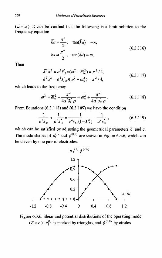
260 Mechanics of Piezoelectric Structures
(a = a). It can be verified that the following is a limit solution to the frequency equation
K ka - — , tan(ka) = -oo,
(6.3.116) K
ka = — , tan(ka) = oo.
Then
k2a2 = a2s^p(co2-co2) = 7r2/4,
k2a2 = a2s'up(o)2 -a2D) = n2l\,
which leads to the frequency 2 2
2 2 ft 1 ft G> =0)x+ r ^ — = G)„ + —
4 o S\\P 4a snp
From Equations (6.3.118) and (6.3.109) we have the condition
1 1 1 • + •
1
c 544 a 5U c 544(1-Ar15) a sn
(6.3.117)
(6.3.118)
(6.3.119)
which can be satisfied by adjusting the geometrical parameters c and c.
The mode shapes of Wj(1) and ^ ( 0 0 ) are shown in Figure 6.3.6, which can
be driven by one pair of electrodes.
„ (i) M(o,o)
-1.2 -0.8 -0.4 0.4 0.8
JC Ja
1.2
Figure 6.3.6. Shear and potential distributions of the operating mode
( c < c ) . M](1) is marked by triangles, and ^(0'0) by circles.
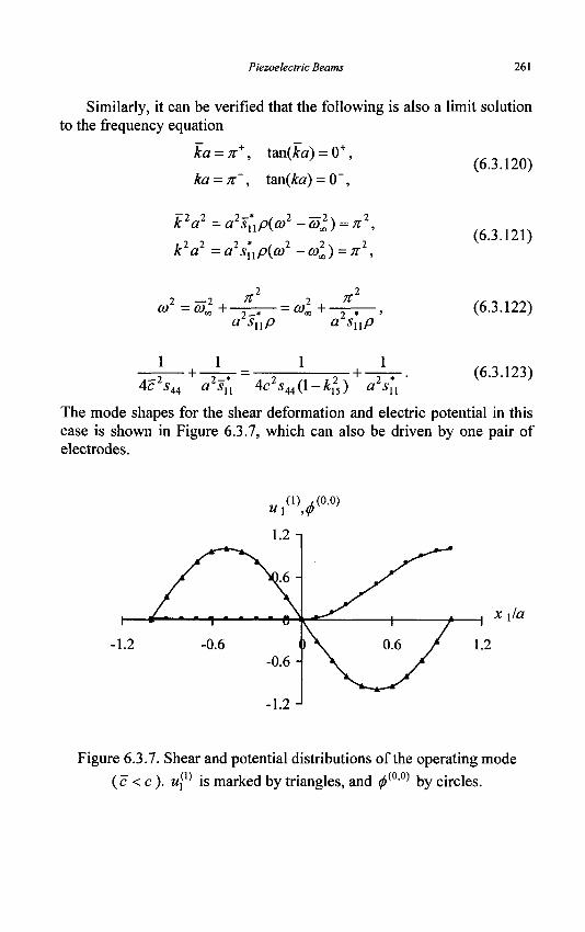
Piezoelectric Beams 261
Similarly, it can be verified that the following is also a limit solution to the frequency equation
ka = n+, tan(£a) = 0+ ,
ka = x~, tan(£a) = 0~, (6.3.120)
k a =a snp{a> -<a^) = K ,
k a =a snp(a> -cox) = n , (6.3.121)
2 —2 #" 2 - * = co„ +-
#
a 5„/7 (6.3.122)
1 1 • + •
1 1
4cz544 als*n 4 : ^44(1 — Ar,25) a2s'u
The mode shapes for the shear deformation and electric potential in this case is shown in Figure 6.3.7, which can also be driven by one pair of electrodes.
„ (i) AOfi) U\ ,(/>
x \la
Figure 6.3.7. Shear and potential distributions of the operating mode
(c <c). w,(1) is marked by triangles, and ^ ( 0 0 ) by circles.
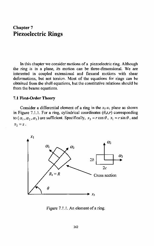
Chapter 7
Piezoelectric Rings
In this chapter we consider motions of a piezoelectric ring. Although the ring is in a plane, its motion can be three-dimensional. We are interested in coupled extensional and flexural motions with shear deformations, but not torsion. Most of the equations for rings can be obtained from the shell equations, but the constitutive relations should be from the beams equations.
7.1 First-Order Theory
Consider a differential element of a ring in the x$-x\ plane as shown in Figure 7.1.1. For a ring, cylindrical coordinates (6^,r) corresponding to ( ax, a2, «3) are sufficient. Specifically, x3 =r cos 0, xx = r sin 0, and
i , « 2
«3
2c
Cross section
* 3
Figure 7.1.1. An element of a ring.
262
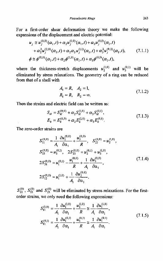
Piezoelectric Rings 263
For a first-order shear deformation theory we make the following expansions of the displacement and electric potential:
Uj s uf0) (a i ,0 + a2uf0) (ax,/) + a3ufA) (a,,t)
+ aluf0) (a,, 0 + a 2 « 3 MJU) («,, /) + a2i/}°-2) (a,, /), (7.1.1)
^ s <*(0'0) (a,, 0 + «2^(1-0) ( a , ,0 + a3^(0',) (a,, /) ,
where the thickness-stretch displacements u2'0^ and Wj0' will be
eliminated by stress relaxations. The geometry of a ring can be reduced from that of a shell with
Ax =R, A2= 1,
Rx =R, R2 = oo.
Then the strains and electric field can be written as:
Ski-Ski' + aiSki' +aiSkt' ,
Ek=E?»+a2Er+a3Er.
The zero-order strains are
(7.1.2)
(7.1.3)
1 duf ,(0,0) , ,(0,0) ~(0,0) _ 1 « ^ 1 « 3 0,(0,0) _ (1,0)
4, oa, R C(0,0) _ (0,1) 9 r,(0,0) _ (0,1) (1,0)
33 — 3 ' ^ 2 3 — 2 3 '
,,(0,0) i a,.(0,0) (7.1.4) 2^(0,0) = M(o,i) _Jf\ +
i au3 \<•'•-*> R Ax da,
Ax da,
Sf2 , S$ and Sf$ will be eliminated by stress relaxations. For the first-order strains, we only need the following expressions:
r _ i dur, 4» = i dur t Ax dax R Ax dax
.m i dur *r„ i r (7'L5) «ii — _ — : — i — z — = • Ax dax R Ax da
264 Mechanics of Piezoelectric Structures
The rest of the first-order strains will be eliminated by stress relaxations. The relevant electric fields are
£(0,0) = _ i _ ^ _ ; £(o,o) = ^(i,o) ^ ^(0,0) = _^(o,i) s
Ax dax
£ ( , , 0 ) = _ _ l _ M ! l j Eil-0)=0, E™=0, (7.1.6) Ax dax
E\ W ) = _ J _ ^ _ , £ f i ) = o, £|0-1>=0. Ax dax
The equations of motion and the charge equations are
R
and
1
A l
A l
dtfii dax
8Ql2 dax
dQn
+ F^=Apbcu^\ (7.1.7)
-Nxx- + F^=Apbcuffi\ Ax dax
u R 3 H 3
_ L ^ r _ e i 2 + F ( , o ) = i ^ , a . o ) ;
^ 5a, 3
J, 5a, ^13 ' 3 ' '
1 5A(0'0) 1 ] _ + ±/)(o,o)+jD(o,o)=() ; Ax dax R
1 SA(1>0) 1 ^ 5a, i?
_ 1 _ S ^ + 1 (o.i) _ ^(0.0) +jD(o,D = 0 j
4 3a, i?
(7.1.8)
] _ + i.Z)0.o) _^(o.o) +Z)0,o) = 0 ; ( 7 j 9 )
Piezoelectric Rings 265
where the resultants are defined by
{Nn,Qn,Qn} = {T$\T$\T^}=\TijdA,
M{m,n) =T(m,n) = f J ^ " ^ (7.1.10) JA
Df* = lAD,a;a;dA.
A = Abe is the cross sectional area. The surface and body loads are
Fjm-n) =bm [c[T2J(b)-(-lTT2j(-b)]a?da3
+ cn £b[T3j(c)-(-iyT3j(-c)]a?da2
+ £ pfrfa^dA, (7.1.11)
/)<»•»>=&» [[D2(b)-(-l)mD2(-b)]a^a3
+ c" £ [D3 (c) - (-1)" D3 (-c)]a?da2.
The constitutive relations are the same as those in the first-order theory of beams
T™ = AbcdS'^S^ --e'^rh a,p = 1,5,6,
Tr=^(cusr-ekAmx
Tr=^f(cnsr-enEr),
(7.1.13)
(7.1.14)
266 Mechanics of Piezoelectric Structures
Ca0~Caf) CaXClftCftfi' eia~eia ei/jCfdCAa>
*ik = £,k + e u c l i % » <x>P = !>5>6> ^ /">v = 23,4, (7.1.15)
_ _ ] _ _ e ^ _ _ T dndkX '-ll ~ ' eil _ ' bik~ bik
With successive substitutions, Equations (7.1.7) through (7.1.9) can be written as eight equations for Ml
(0-0), uJQfi\ uf'°\ Ml(1'0), u^\ f'°\ f'0)
and 0((U). For end conditions we can prescribe
7;(0'0) or Ml(0'0), 7f'0) or uf'°\ 7f°> or uf'°\
T™ or M,(,'0), T™ or u™, (7.1.16) (o.o) o r A(o.o)5 ^o.o) o r Dp.o)> ^(o,D o r A(o,i)_
7.2 Classical Theory
The classical theory for flexure can be obtained from the first-order theory by two approximations, i.e., dropping the rotatory inertia and making the shear strains vanish. The resulting equations are
_ L ^ i L + a I + F/o.o) =4pbcii[0'°\ Ax dax *u R ' H !
1 M2+F(o,o)=4pbcUio,o)^ ( 7 2 1 )
Ax dax
I ^ L _ J V I + F M =4p6c«<0-0>,
1 9A(0'0) 1 M 3
Ax dax R +-z>r)+z)(0'0)=o,
LdD?'0) + 1/jO.o) _^(0.0) + ^(1.0) = 0> ( ? 2 2 )
Ax dax R
_LdD?'l) + I/)(0.1) _ D(0.0) + £(0,1) = Qj
.4, 9a, /?
Piezoelectric Rings 267
T^ =Abc{c[xS[0fi) -e'aEffi)\
A(0'0)=4M?^r0)+44°'0))>
Tr=^(cnsr-ekiEr),
^=^f(cusr-enErx
1 d,A0^ iA°'0) e(0,0) _ l ou\ , «3
" 1 1 — — : <
Ax dax R
CO.O) „ X ° " l o(0,l) ^ 1 C"l t j j j = , i 3 j , =
Al da, Ax da,
(7.2.3)
(7.2.4)
(7.2.5)
1 / W ( 1 , 0 ) 1 r)MW)
Qn=^r-^-^r, Qn-y-^-^r, (7.2.6) Y4, oa, .4, oa,
(7.2.7)
M(i.o) = _ _ L ^ 1 _ 5 (o.i) = _ J_^^ + ii_ ( 7 2 8 )
4, 5a, yij 5a, i?
With successive substitutions, Equations (7.2.1) and (7.2.2) can be written as six equations for Ml
(0'0), u2m, uffi), f'°\ f'0) and f». For
end conditions we can prescribe
7f-0) or Ml(0-0), 4°-0) or uf°\ T^0) or Mf0),
fl,.(0,0) = (0,0)
70 .0 ) o r ^ 2 _ 9 ^(0,1) Q r ^ _ ( 7 2 8 )
3a, 9a, 0<o.o) o r A (o > 0 ) ) 0(i;o) o r A ( . , o ) ; 0(0,1) o r A(o,i) _
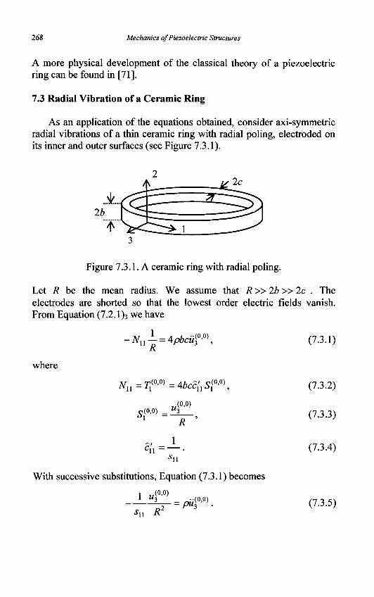
268 Mechanics of Piezoelectric Structures
A more physical development of the classical theory of a piezoelectric ring can be found in [71].
7.3 Radial Vibration of a Ceramic Ring
As an application of the equations obtained, consider axi-symmetric radial vibrations of a thin ceramic ring with radial poling, electroded on its inner and outer surfaces (see Figure 7.3.1).
Figure 7.3.1. A ceramic ring with radial poling.
Let R be the mean radius. We assume that R»2b»2c . The electrodes are shorted so that the lowest order electric fields vanish. From Equation (7.2.1)3 we have
where
1 (0,0) -Nu — = 4pbcu3
Ni^TW^tbcc^S™,
£(0,0) .(0,0) h
R
(7.3.1)
(7.3.2)
(7.3.3)
(7.3.4)
With successive substitutions, Equation (7.3.1) becomes
1 7/°>0)
>n IT (7.3.5)
Piezoelectric Rings
For time-harmonic motions, the frequency is given by
psuR2
which is the same as the result given in [9].
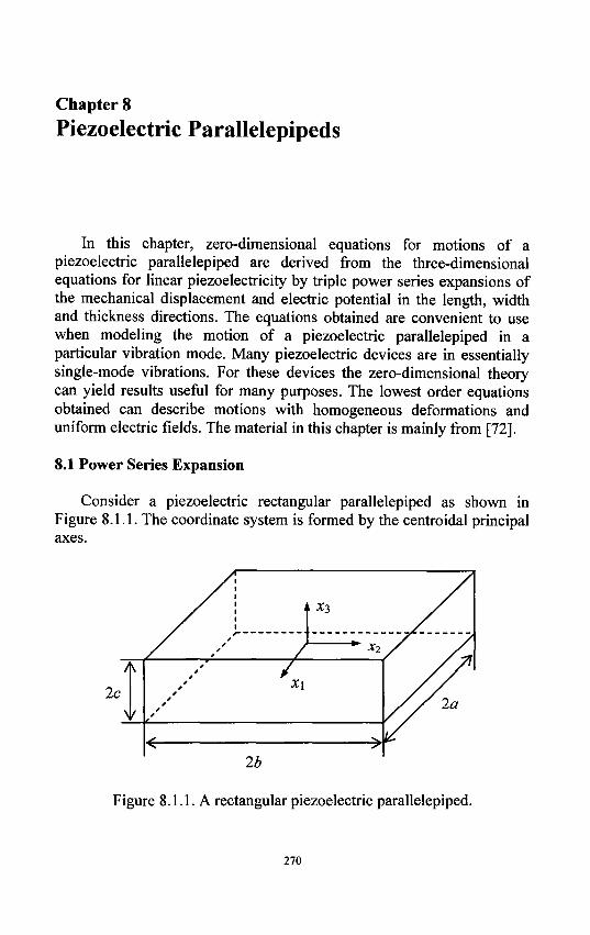
Chapter 8
Piezoelectric Parallelepipeds
In this chapter, zero-dimensional equations for motions of a piezoelectric parallelepiped are derived from the three-dimensional equations for linear piezoelectricity by triple power series expansions of the mechanical displacement and electric potential in the length, width and thickness directions. The equations obtained are convenient to use when modeling the motion of a piezoelectric parallelepiped in a particular vibration mode. Many piezoelectric devices are in essentially single-mode vibrations. For these devices the zero-dimensional theory can yield results useful for many purposes. The lowest order equations obtained can describe motions with homogeneous deformations and uniform electric fields. The material in this chapter is mainly from [72].
8.1 Power Series Expansion
Consider a piezoelectric rectangular parallelepiped as shown in Figure 8.1.1. The coordinate system is formed by the centroidal principal axes.
Figure 8.1.1. A rectangular piezoelectric parallelepiped.
270
Piezoelectric Parallelepipeds 271
To develop a zero-dimensional theory, we make the following expansions of the mechanical displacement vector and the electrostatic potential:
uj (*, ,x2,x3,t) = £ x[x^xn,ufm'n) (0, l,m,n=0
</>(Xi, x2 ,x3, t) = ]T xix^xn3^'-m'n) (t).
I,m,n=0
Then the strains and the electric field can be written as
C _ V v ' v « v " c(',m,n)
l,m,n=0
where
l,m,n=0
sy**) =I[(/+i)(^ lMy+i'm>" )+snu\M>m>n))
Ef'm'n) =-Sn{l + \)f+x'm-n)
- Si2 (m + l)^(/'m+1'") - Sa (n + X)^"^.
(8.1.1)
(8.1.2)
+ (m + l)(Snufm+l'n) + SJ2u«-m+1-n)) (8.1.3)
(8.1.4)
Substituting Equation (8.1.1) into the variational formulation of linear piezoelectricity in Equation (1.2.26), with integration by parts, for
independent variations of Sufm,n) and S0(-''m,n), we obtain the following
zero-dimensional equations of motion and electrostatics:
_lT(l-\,m,n) _mTV,»-l,n) _nTV*>*-*>
+ F?'m* = P £ * / + m , « + ^ W ) > (8-1-5) p,q,r=0
_lD(l-Um,n) _mDV*-U) _nD(l,n>,n-\) +D(.l,m,n) = ^
272 Mechanics of Piezoelectric Structures
where the stress and the electric displacement of various orders are defined by
2j'-"-"> = I TijX[x^x"3dV,
(8.1.6)
V = Sabc is the volume of the parallelepiped. Surface traction, surface charge and body force of various orders have the following expressions:
p(l,m,n) _ j(l,m,n) + ~f(l,m,n)
Tj''m'n) = Ldx2 £«k 3 Pi , (* i = « ) - ( - ! ) % ( * . =-a)]a'x!?x"3
+ J[ dxx £dx3[T2J (x2 =b)- (-l)m T2J (x2 = -b)]bmx[x"z (8.1.7)
+ [jx, lbdx2[Ty{x, = c ) - ( - l ) % ( x 3 = -c)]cnx[x'2n,
/,<'•"•"> = I ffjtexSdV,
DU,m,n) = j * <fe2 £ <&3[D,(JC, =a)-(-Y)'Dl(xl =-a)]a'jc2mx3"
+ f * i f ^ 3 [^2(^2 =6)-(-l)",-D2(-3c2 =-A)]*"^'*" (8.1.8)
+ f A , [* <k2[Z>3(*3 =c ) - ( - l ) "D 3 (x 3 = -c)]c"*1'*2". J-a J-b
Bi+P,m+q,n+r is a geometric quantity defined by
D _ f rl+Pr
m+ix"+rdV
nl+p,m+q,n+r~ ]y x\ x2 x3 a v
Sa'+p+1b'n+',+lc"+r+l , (8.1.9)
(l + p + \)(m+q + \)(n + r + \) 0, else.
, 1 + p,m + q,n + r even,
Piezoelectric Parallelepipeds 273
The zero-dimensional constitutive relations are 00
T(l,m,n) _ " V D / „ v(p,q,r) f(P,qs)\ 1ij - / .•Dl+D.m+a.n+r\ciikli:>kl ekijnk h
P,q,r=0
00
/ ) ( ' • '»• '")_ V 1 D /> c(P,?,'-) , «, F<.P.<l.r)\ u i ~ / 1
J}l+p.m+a.n+r\eiklc>kl + bik£'k )> P,q,r=0
or, with the compact matrix notation, for M, N = 1, 2, ..., 6 00
T(l,m,n) _ V"1 R , a(p,q,r) p<.P,9,r)\
1M ~ J£Jnl+p,m+q,n+r\cMNL3N ^kM^k h
p,q,r=o
(8.1.10)
(8.1.11)
- ^ i _ / .Dl+Djn+gjn+r\eiNAN +EiktLk )•
p,q,r=o
With successive substitutions, these equations can be written as ordinary differential equations for the mechanical displacements and electric potentials of various orders.
8.2 Zero-Order Equations
We keep u<°- °'0), W?-0-°\ Mf'-0>, a f 0 ^ , ^°-°>, ^ W , and ^ w \
and neglect all higher order displacements and potentials. For (l,m,n) = (0,0,0), (1,0,0), (0,1,0) and (0,0,1), we have the following equations of motion and electrostatics:
F™ = p$abcu?>°'°\ £(0.0.0) = 0 >
(8.2.1)
. j(o,o,o) + ^0,0,0) _ 8a be „(1A0) ly y 3 J' ' (8.2.2)
_n(o.o.o)+ 2)0.0.0) = Q '\
_r(OAO)+F(o,i,o)= 8a^£„(0,1.o) 7 v 3 J ' (8.2.3)
-£>f°-0)+Z)(0-1-0)=0,
274 Mechanics of Piezoelectric Structures
_r(o,o,o) E,(O,O,I) = %abc (0>0il) 3) j 3 7 '
_Z)(o,o,o)+£)(o,o,i)=0
The constitutive relations for the above equations are
Drfi)=Sabc(eiNSr'0)+eikEr'0)),
in which the zero-order strains and electric fields are given by
^(0 ,0 ,0) _ M(l,0,0) £,(0,0,0) _ M(0,0,l) + M(0,l ,0)
£•(0,0,0) _ M(0,l,0) £,(0,0,0) _ M(l,0,0) + u (0 ,0 , l )
0(0,0,0) _ (0,0,1) o(0,0,0) _ (0,1,0) (1,0,0)
i 3 3 — M3 , i 3 6 — Wj + M 2 >
£(o,o,o) = _ (i,o,o) 5 £(o,o,o) = _ (o,i,o) £(o,o,0) = _ (o,o,i) _ ( 8 2 J )
These equations can be written as equations for uj°'°'0), uf'0,0^, «j0 '1,0),
M(o,o,i) (i,o,o) (o,i,o) a n d 0(o,o,i) w h i c h g o v e m t h e r i g i d b o d y m o t i o n 5
homogeneous stretching and shearing deformations of the parallelepiped and uniform electric fields.
8.3 A Piezoelectric Gyroscope
As an application of the zero-dimensional theory developed above, we revisit the thickness-shear ceramic plate piezoelectric gyroscope analyzed in the fourth section of the second chapter. Consider the rectangular ceramic plate shown in Figure 8.3.1.
The plate is poled in the thickness direction. A driving voltage V\ is applied across the lateral electrodes at x\ = ±a to excite the plate into thickness-shear motion u\ in the x\ direction. When the plate is rotating about the x3 axis, the Coriolis force F2 causes a thickness-shear motion u2
in the x2 direction. This shear in the x2 direction generates a voltage V2
between x2 = ±b, which can be used to detect the angular rate Q.
(8.2.4)
(8.2.5)
(8.2.6)
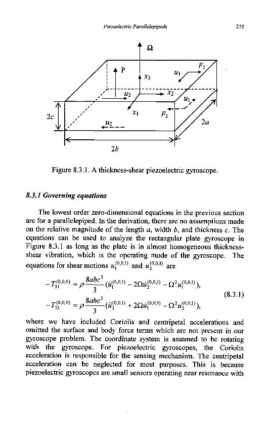
Piezoelectric Parallelepipeds 275
Figure 8.3.1. A thickness-shear piezoelectric gyroscope.
8.3.1 Governing equations
The lowest order zero-dimensional equations in the previous section are for a parallelepiped. In the derivation, there are no assumptions made on the relative magnitude of the length a, width b, and thickness c. The equations can be used to analyze the rectangular plate gyroscope in Figure 8.3.1 as long as the plate is in almost homogeneous thickness-shear vibration, which is the operating mode of the gyroscope. The equations for shear motions u[°'QX> and uf'0^ are
_7-3(0.0.0) = p 8 a ^ ( „ ( 0 > 0 , 1 ) _ 2 Q j i (o ,o , i ) _ Q 2 W ( O , O , I ) X
3 3 (8-3.1)
-^o.o.o) =/,8a6c_(„(0,o,1) +2Qti(o,o,D _Q2M(o,o,i)x
where we have included Coriolis and centripetal accelerations and omitted the surface and body force terms which are not present in our gyroscope problem. The coordinate system is assumed to be rotating with the gyroscope. For piezoelectric gyroscopes, the Coriolis acceleration is responsible for the sensing mechanism. The centripetal acceleration can be neglected for most purposes. This is because piezoelectric gyroscopes are small sensors operating near resonance with
276 Mechanics of Piezoelectric Structures
high frequencies. Usually Q, is much smaller than the operating frequency. Therefore the centripetal acceleration, the third terms on the right hand sides of Equation (8.3.1)i2, which are quadratic in Q, are small compared with the Corioils acceleration, the second terms of the equations. The relevant constitutive relations take the following form:
r3r-o)=*abc(c4ysr-o) - e15KEro)),
Dr0)^abc(el5KSr'0)+euErfi)),
Z)f°-0) =Sabc(el5KS<0fifi) + * 1 1 £ 2m o ) ) .
In Equations (8.3.2) and (8.3.3) we have introduced a thickness-shear correction factor K to compensate for the error caused by truncating the
series. For a ceramic plate we have K2 = n2 /12 when the plate is poled in the thickness direction. For convenience we introduce the notation
Then
u{0M=U„ u2°M=U2,
^°'0)=Vl/2a, <f>(0X0)=V2/2b.
s?-°v=u2, sfA0)=uu E™=-Vx/2a, E^0fi)=-V2/2b.
With successive substitutions, we obtain
-CAAK2UX -eX5KVx /2a = p—(Ul -2QU2 - Q 2 ^ ) .
c 2 -C44K
2U2 -e15KV2 I2b = p—{U2 + 2QC/, -Q2U2),
(8.3.4)
(8.3.5)
(8.3.6)
(8.3.7) Df'm = %abc(el5KUx -enVx 12a),
D?A0) =Sabc(el5nU2 -enV2 12b).
The total electric charge on the electrodes at x\ = a or xi = b and the electric currents flowing out of them are given by
ft = -A(°'°'0) «2a), Q2 = -Drfi) H2b), ( 8 3 8 )
/ , = - & , I2=-Q2.
Piezoelectric Parallelepipeds 277
The driving voltage V\ is usually considered known and is time-harmonic. The sensing electrodes at x2 = ±b are usually connected by an output circuit with impedance Z for harmonic motions. In the special cases when Z = 0 or oo, we have short or open output circuit with V2 = 0 or I2 = 0. In general, neither V2 nor I2 is known and a circuit equation is needed. Let the known time-harmonic driving voltage be Vx = iVx exp(/6rf) . Introducing the complex notation
Ux = iUx expQwt), U2 = U2 exp(ioX),
I2 = I2 exp(/6rf), V2 = V2 exp(ia>t),
we can write the circuit condition as
I2=V2/Z. (8.3.10)
From Equations (8.3.7)2, (8.3.8)2,4 and (8.3.10), we obtain
4acico(el5tdJ2 -euV2 /2b) = V2/Z. (8.3.11)
Then we have the following equations:
-C4 4K-2£/, -eXiKVx 12a
c2 — — — = p—{-(Q2UX -2QcoU2 -Q2UX),
-C44K2U2 -eX5KV2 12b (8.3.12)
r2 — — — = p—(-co2U2 -2Qo>Ux -n2U2),
4ac<a(el5KU2 -sxxV2 12b) = V2 /iZ(co).
Equation (8.3.12) represent three linear algebraic equations for Ux, U2
and V2 in which Vx is the inhomogeneous driving term. In general Z is a
function of a>. The specific form of this function depends on the structure of the load circuit.
8.3.2 Free vibration
For free vibrations we set Vx = 0 , which physically means that the driving electrodes are shorted. Then Equation (8.3.12) reduces to a system of homogeneous equations for Ux, U2 and V2. For nontrivial
278 Mechanics of Piezoelectric Structures
solutions, the determinant of the coefficient matrix must vanish, which leads to the following frequency equation:
A(o)) = (G)2 +Q2 -col)2
- 4Q2co2 - X((D)CDI {a1 + Q2 - <y2) = 0, (8.3.13)
where we have denoted
2 3 c 4 4 y 3 / - , \ _ *T5
pc 1 + Z2(CO)/Z(G))
2 (8.3.14)
lr2 __fi5__ 7 _ 1 - _£n4ac £uc44 i<yC2 2o
<yw is the lowest thickness-shear resonant frequency of an elastic plate with shear constant c44, mass density p, and thickness 2c. The correction factor K makes this frequency to be the same as that obtained from the three-dimensional equations. k2
5 is an electro-mechanical coupling factor that represents the strength of this coupling of the material. Cj is a static capacitance. Equation (8.3.13) can be written in the following form:
co2 = ( 1 - 4 ^ + 0 ' ±Uco2xJl + ^ ^ - • (8.3.15)
2 2 \ X coK
Strictly speaking, Equation (8.3.15) is not a frequency solution to Equation (8.3.13) because, in general, A is a function of co. In the special case of shorted output electrodes we have Z = 0, A = 0. Then Equation (8.3.15) reduces to
co = (oa,±n, (8.3.16)
which is a frequency solution. When the output electrodes are open we have Z = °°, A = k2
5. In this case Equation (8.3.15) also represents a frequency solution. Piezoelectric gyroscopes usually operate under the condition that Q « cox. From Equation (8.3.15) we can see that, for small Q, and open output electrodes, the effect of Q on co is quadratic. This is different from the special case of shorted output electrodes as shown by Equation (8.3.16). If the load circuit is essentially capacitive with a capacitance C, we have Z = \l{icoC) and Z2IZ = C/C2 which is independent of CO. Then Equation (8.3.15) represents a frequency solution.
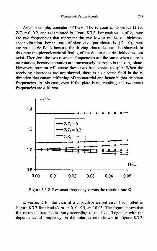
Piezoelectric Parallelepipeds 279
As an example, consider PZT-5H. The relation of ft) versus Q, for Z/Z2 = 0, 0.2, and °° is plotted in Figure 8.3.2. For each value of Z, there are two frequencies that represent the two lowest modes of thickness-shear vibration. For the case of shorted output electrodes (Z = 0), there are no electric fields because the driving electrodes are also shorted. In this case the piezoelectric stiffening effect due to electric fields does not exist. Therefore the two resonant frequencies are the same when there is no rotation, because ceramics are transversely isotropic in the X\-X2 plane. However, rotation will cause these two frequencies to split. When the receiving electrodes are not shorted, there is an electric field in the x2
direction that causes stiffening of the material and hence higher resonant frequencies. In this case, even if the plate is not rotating, the two shear frequencies are different.
1.4
1.2
0.8
co/a>a
— Z/Z2 = 0
-*-ZIZ2 = 0.2
—~Z/Z2 = °°
QJa>«
0.00 0.01 0.02 0.03 0.04 0.05
Figure 8.3.2. Resonant frequency versus the rotation rate Q.
0) versus Z for the case of a capacitive output circuit is plotted in Figure 8.3.3 for fixed Q/mx = 0, 0.025, and 0.05. The figure shows that the resonant frequencies vary according to the load. Together with the dependence of frequency on the rotation rate shown in Figure 8.3.2,
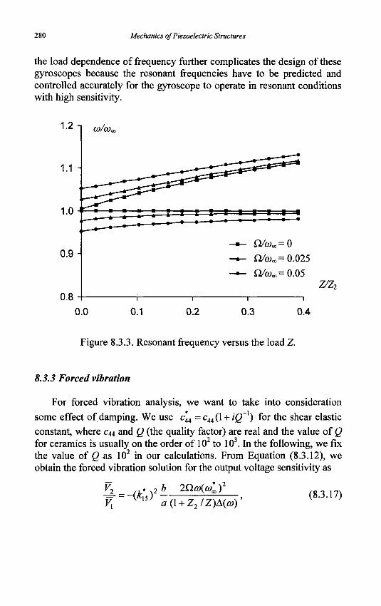
280 Mechanics of Piezoelectric Structures
the load dependence of frequency further complicates the design of these gyroscopes because the resonant frequencies have to be predicted and controlled accurately for the gyroscope to operate in resonant conditions with high sensitivity.
1.2
1.1
1.0
0.9
0.8
CO/COa,
j , * * -—* *' —« • » »
I
1 1 - I — 1 1 1 _ • » » • « •
- * - n/coM=o - • - Q/(ox= 0.025
- ^ Q/com= 0.05
i i
ZJZr
0.0 0.1 0.2 0.3 0.4
Figure 8.3.3. Resonant frequency versus the load Z.
8.3.3 Forced vibration
For forced vibration analysis, we want to take into consideration
some effect of damping. We use c*44 = c44(l + iQ~x) for the shear elastic
constant, where c44 and Q (the quality factor) are real and the value of Q for ceramics is usually on the order of 102 to 103. In the following, we fix the value of Q as 102 in our calculations. From Equation (8.3.12), we obtain the forced vibration solution for the output voltage sensitivity as
-=- = -(*15) ' b 2Q^(^M)2
a(\ + Z2/Z)A(<0) (8.3.17)
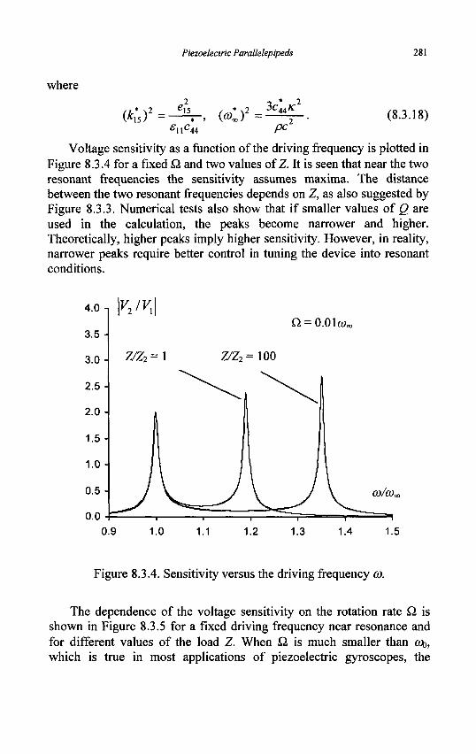
Piezoelectric Parallelepipeds 281
where
(*i5)2=-= 15
£,,c ll t '44
, * \2 3 C 44 y
PC (8.3.18)
Voltage sensitivity as a function of the driving frequency is plotted in Figure 8.3.4 for a fixed Q. and two values of Z. It is seen that near the two resonant frequencies the sensitivity assumes maxima. The distance between the two resonant frequencies depends on Z, as also suggested by Figure 8.3.3. Numerical tests also show that if smaller values of Q are used in the calculation, the peaks become narrower and higher. Theoretically, higher peaks imply higher sensitivity. However, in reality, narrower peaks require better control in tuning the device into resonant conditions.
Q = 0.01cya
Figure 8.3.4. Sensitivity versus the driving frequency (O.
The dependence of the voltage sensitivity on the rotation rate Q is shown in Figure 8.3.5 for a fixed driving frequency near resonance and for different values of the load Z. When Q. is much smaller than a>o, which is true in most applications of piezoelectric gyroscopes, the
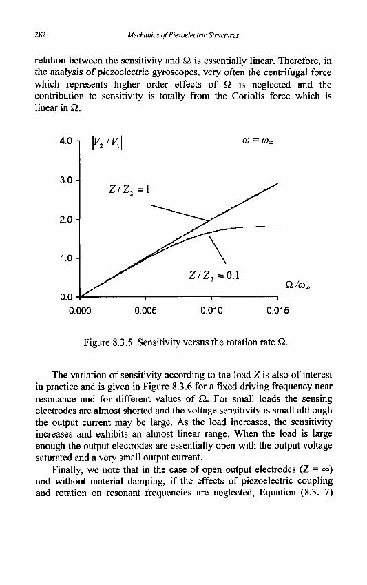
282 Mechanics of Piezoelectric Structures
relation between the sensitivity and Q is essentially linear. Therefore, in the analysis of piezoelectric gyroscopes, very often the centrifugal force which represents higher order effects of Q is neglected and the contribution to sensitivity is totally from the Coriolis force which is linear in Q,.
4.0 -i
3.0-
2.0 -
1.0-
0.0-
\v iv\ V 2 ' y\\
ZIZ2 = 1
1
CO = OJoo
Z/Z2 =0.1
1 1
Q/a>a
0.000 0.005 0.010 0.015
Figure 8.3.5. Sensitivity versus the rotation rate Q.
The variation of sensitivity according to the load Z is also of interest in practice and is given in Figure 8.3.6 for a fixed driving frequency near resonance and for different values of Q.. For small loads the sensing electrodes are almost shorted and the voltage sensitivity is small although the output current may be large. As the load increases, the sensitivity increases and exhibits an almost linear range. When the load is large enough the output electrodes are essentially open with the output voltage saturated and a very small output current.
Finally, we note that in the case of open output electrodes (Z = °°) and without material damping, if the effects of piezoelectric coupling and rotation on resonant frequencies are neglected, Equation (8.3.17)
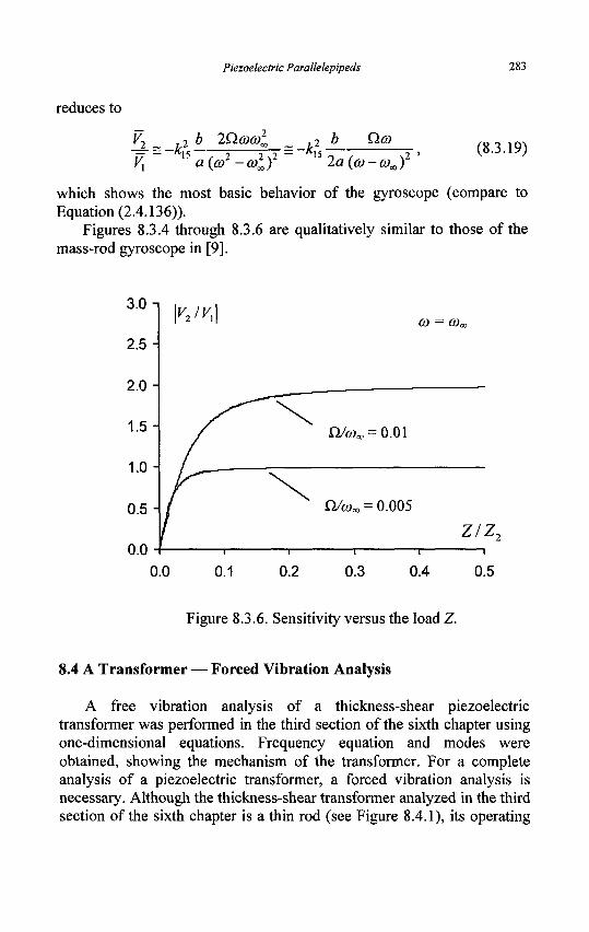
Piezoelectric Parallelepipeds 283
reduces to
S^A4^^_4±_^L_, (8.3.19) Vx
i5 a(co2-coif X52a(co-wJ
which shows the most basic behavior of the gyroscope (compare to Equation (2.4.136)).
Figures 8.3.4 through 8.3.6 are qualitatively similar to those of the mass-rod gyroscope in [9].
3.0-
2 .5 -
2.0-
1.5
1.0
0.5
0.0
0.0 0.1 0.2 0.3 0.4 0.5
Figure 8.3.6. Sensitivity versus the load Z.
8.4 A Transformer — Forced Vibration Analysis
A free vibration analysis of a thickness-shear piezoelectric transformer was performed in the third section of the sixth chapter using one-dimensional equations. Frequency equation and modes were obtained, showing the mechanism of the transformer. For a complete analysis of a piezoelectric transformer, a forced vibration analysis is necessary. Although the thickness-shear transformer analyzed in the third section of the sixth chapter is a thin rod (see Figure 8.4.1), its operating
co = co„
Q/eOo, = 0.005
ZIZ,
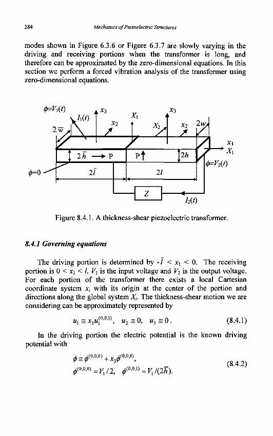
284 Mechanics of Piezoelectric Structures
modes shown in Figure 6.3.6 or Figure 6.3.7 are slowly varying in the driving and receiving portions when the transformer is long, and therefore can be approximated by the zero-dimensional equations. In this section we perform a forced vibration analysis of the transformer using zero-dimensional equations.
0=^(0
Figure 8.4.1. A thickness-shear piezoelectric transformer.
8.4.1 Governing equations
The driving portion is determined by -/ < jti < 0. The receiving portion is 0 < x\ < I. V\ is the input voltage and V-i is the output voltage. For each portion of the transformer there exists a local Cartesian coordinate system JC, with its origin at the center of the portion and directions along the global system Xt. The thickness-shear motion we are considering can be approximately represented by
.x3ux
(0,0,1) u2 = 0, w3 = 0. (8.4.1)
In the driving portion the electric potential is the known driving potential with
0(o.o,o) =vl2f ^o.o.i) =v/(2hy (8.4.2)
Piezoelectric Parallelepipeds 285
From Equation (8.2.4)i, setting j = 1, we obtain the equation of motion as
. ^ 0 . 0 . 0 ) + ^(0,0,.) = p ^ g ( 0 A i ) ; (g.4.3)
where
(0.0.1) = r f Tn{x = 0-)X3dX2dX3. (8.4.4) J-w J-h
(8.4.5)
Relevant constitutive relations are taken from Equation (8.2.5)
T$fifi) =mh{c„K2S?fi>0) -e15K£3(0A0)),
In Equation (8.4.5) we have introduced a thickness-shear correction factor K. For a ceramic parallelepiped we can use K2 = n21\2 as an approximation. For the charge and current on the electrode at X^ = h, we have
Q,=-D?^l(2h), /,=-e,. (8.4.6)
In the receiving portion, the electric potential can be written as
<f>(0A0) = V2/2, <?>iW)=V2/(2l), (8.4.7)
2 ' *-> r ~'i>
where V2 is unknown. The equation of motion is
_T(0A0)+F(0M=p^Lu(0M^ ( 8 4 8 )
where eh
F](o,o,.) T f -Tu(X,=V)X,dX2dX,. (8.4.9) J-w J-h
(8.4.10)
Relevant constitutive relations are
T ™ =&lwh(cuK2S^°-0) -e15KEr>0)),
The electric charge on the electrode at X\ - 21 and the electric current flows out of the electrode are given by
Q2=-Drfi)K2l), I2=-Q2. (8.4.11)
286 Mechanics of Piezoelectric Structures
In deriving the above we have assumed that there is no body force and made use of the traction-free boundary conditions at X\ = 21, X2 = ±w, andX3 = ±/j.
Substituting Equation (8.4.10)i into Equation (8.4.8), and Equation (8.4.5)i into Equation (8.4.3), adding the resulting equations and making use of the continuity conditions
F1(0 '°'I)(^1=0-) = -F1
(0-0 '1)(^1=0+),
M 1 ( Z 1 = 0 - ) = W I ( ^ 1 = 0 + ) ,
we obtain
(8.4.12)
= ^p(hvh3+Jwh3yul0Al).
-&wh(cA4K2S?m -ei5KE?A0)) (8.4.13)
3 '
Under the known time-harmonic driving voltage Vx = Vx exp(icot), for
time-harmonic solutions we employ the complex notation and write the unknowns as
u[0A1) = u exp(/fttf), V2 = V2 exp(/<s#), (8 4 14)
Ix = 7, exp(/6#), Ii - h exp(ifijf).
The receiving electrodes are connected by an output circuit which, when the motion is time-harmonic, has an impedance ZL. We have the following circuit condition
I2=V2/ZL. (8.4.15)
With successive substitutions, we obtain the following two equations for u and V2, driven by Vx
- &lwh(c44K2u + eX5K—) - Slwh(c44K
2u + e15ic—L) 21 2h
= --ptfwh3 +lwh3)(D2u, (8.4.16)
_ V V 4whico(el5KU - sn -M = -*-.
11 LL
Piezoelectric Parallelepipeds 287
Once u and V2 are obtained, the currents are given by
I2 = Awhia>{eX5m -exx — ) , ^ (8.4.17)
Ix = 4lwico(eX5Ku -sxx —^=). 1h
8.4.2 Forced vibration analysis
We consider the case oi 1 = 1 and w = w . Solving Equations (8.4.16) for u and V2, we obtain the transforming ratio and normalized input and output currents as
v2 £ =l Vx (\ + h/h)(\ + Z2/ZL)(o)2leol-Y)-kx\hlh h'
I k2 I 12 _ "15 '
(Vx/Z2) (l + h/h)(l + ZL/Z2)(co2Ico2 -\)-kx\hZLl{hZ2) h
/, = 1 _ k{5(l + Z2/ZL) (Vx/Zx) ' {\ + hlh){\ + Z2IZL){oi210)1-1)-^/^
(8.4.18) where
4 j _ 3A:2C44
fnc44 p(h-hh+h)
Zx=-L., Cx = £-A, (8.4.19)
ityC, 2/?
7 - _ ! _ r - f i i 4 ^ iccC2 21
In Equation (8.4.19), a>x is the thickness-shear resonant frequency for shorted receiving electrodes (ZL = 0) as predicted by the zero-dimensional theory, C\ and C2 are the static capacitance of the driving and receiving portions, and Z\ and Z2 are the impedance of the two portions. As a numerical example, we consider PZT-5H. Material damping is included by allowing cpq to assume complex values. c44 is
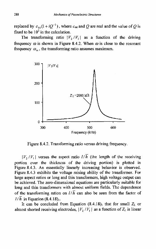
288 Mechanics of Piezoelectric Structures
replaced by c44(1 + iQ x), where c44 and Q are real and the value of Q is fixed to be 102 in the calculation.
The transforming ratio \V2IVX\ as a function of the driving frequency 0) is shown in Figure 8.4.2. When 0) is close to the resonant frequency &>x, the transforming ratio assumes maximum.
300
200
100
IK2/F1
— 1 1
400 500 Frequency (kHz)
300 600
Figure 8.4.2. Transforming ratio versus driving frequency.
\V2IV1\ versus the aspect ratio II h (the length of the receiving portion over the thickness of the driving portion) is plotted in Figure 8.4.3. An essentially linearly increasing behavior is observed. Figure 8.4.3 exhibits the voltage raising ability of the transformer. For large aspect ratios or long and thin transformers, high voltage output can be achieved. The zero-dimensional equations are particularly suitable for long and thin transformers with almost uniform fields. The dependence of the transforming ration on llh can also be seen from the factor of IIh in Equation (8.4.18)1.
It can be concluded from Equation (8.4.18)1 that for small ZL or almost shorted receiving electrodes, V2IVX as a function of ZL is linear
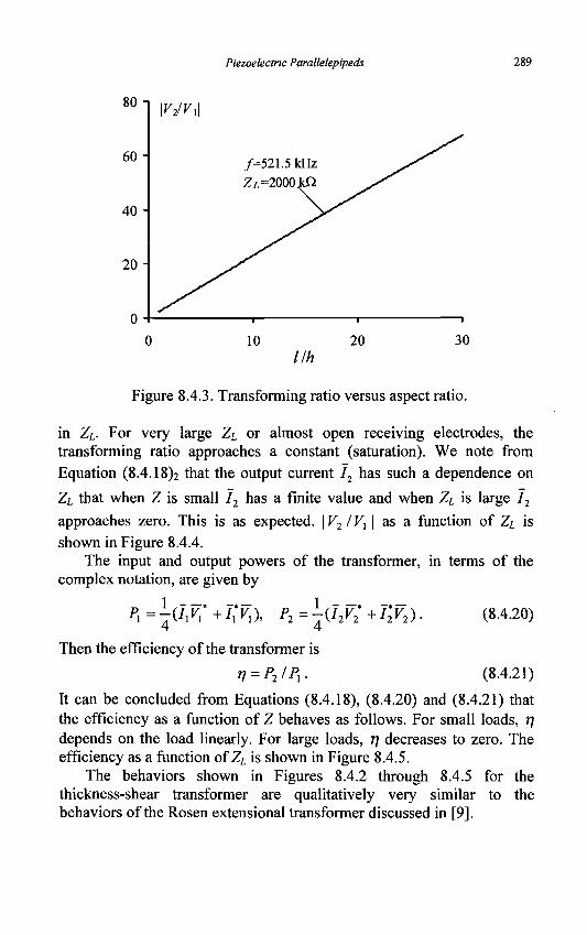
Piezoelectric Parallelepipeds 289
80
60
40
20
\v2ivx\
/=521.5 kHz ZL =2000 J
10
— i —
20
—i
30 llh
Figure 8.4.3. Transforming ratio versus aspect ratio.
in ZL. For very large ZL or almost open receiving electrodes, the transforming ratio approaches a constant (saturation). We note from Equation (8.4.18)2 that the output current I2 has such a dependence on ZL that when Z is small 72 has a finite value and when ZL is large I2
approaches zero. This is as expected. \V2/V] | as a function of ZL is shown in Figure 8.4.4.
The input and output powers of the transformer, in terms of the complex notation, are given by
Px=\(hV'+ixVx\ P2=\(I2V;+r2V2). (8.4.20)
Then the efficiency of the transformer is
r] = P2/Pl. (8.4.21)
It can be concluded from Equations (8.4.18), (8.4.20) and (8.4.21) that the efficiency as a function of Z behaves as follows. For small loads, r\ depends on the load linearly. For large loads, r\ decreases to zero. The efficiency as a function of ZL is shown in Figure 8.4.5.
The behaviors shown in Figures 8.4.2 through 8.4.5 for the thickness-shear transformer are qualitatively very similar to the behaviors of the Rosen extensional transformer discussed in [9].
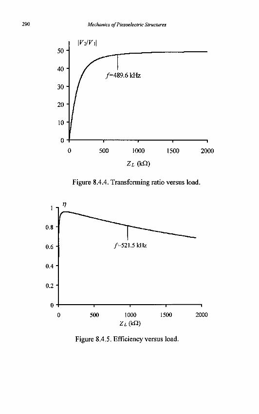
290 Mechanics of Piezoelectric Structures
2000
Figure 8.4.4. Transforming ratio versus load.
1
0.8
0.6 i
0.4
0.2
/=521.5kHz
0
500 1000
ZL (kQ)
1500 2000
Figure 8.4.5. Efficiency versus load.
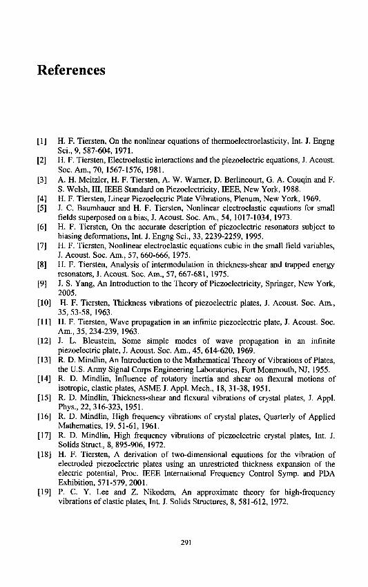
References
[I] H. F. Tiersten, On the nonlinear equations of thermoelectroelasticity, Int. J. Engng Sci., 9, 587-604,1971.
[2] H. F. Tiersten, Electroelastic interactions and the piezoelectric equations, J. Acoust. Soc.Am., 70, 1567-1576, 1981.
[3] A. H. Meitzler, H. F. Tiersten, A. W. Warner, D. Berlincourt, G. A. Couqin and F. S. Welsh, III, IEEE Standard on Piezoelectricity, IEEE, New York, 1988.
[4] H. F. Tiersten, Linear Piezoelectric Plate Vibrations, Plenum, New York, 1969. [5] J. C. Baumhauer and H. F. Tiersten, Nonlinear electroelastic equations for small
fields superposed on a bias, J. Acoust. Soc. Am., 54, 1017-1034,1973. [6] H. F. Tiersten, On the accurate description of piezoelectric resonators subject to
biasing deformations, Int. J. Engng Sci., 33, 2239-2259, 1995. [7] H. F. Tiersten, Nonlinear electroelastic equations cubic in the small field variables,
J. Acoust. Soc. Am., 57, 660-666, 1975. [8] H. F. Tiersten, Analysis of intermodulation in thickness-shear and trapped energy
resonators, J. Acoust. Soc. Am., 57, 667-681, 1975. [9] J. S. Yang, An Introduction to the Theory of Piezoelectricity, Springer, New York,
2005. [10] H. F. Tiersten, Thickness vibrations of piezoelectric plates, J. Acoust. Soc. Am,
35, 53-58, 1963. [II] H. F. Tiersten, Wave propagation in an infinite piezoelectric plate, J. Acoust. Soc.
Am., 35, 234-239,1963. [12] J. L. Bleustein, Some simple modes of wave propagation in an infinite
piezoelectric plate, J. Acoust. Soc. Am., 45, 614-620,1969. [13] R. D. Mindlin, An Introduction to the Mathematical Theory of Vibrations of Plates,
the U.S. Army Signal Corps Engineering Laboratories, Fort Monmouth, NJ, 1955. [14] R. D. Mindlin, Influence of rotatory inertia and shear on flexural motions of
isotropic, elastic plates, ASME J. Appl. Mech., 18, 31-38,1951. [15] R. D. Mindlin, Thickness-shear and flexural vibrations of crystal plates, J. Appl.
Phys., 22, 316-323, 1951. [16] R. D. Mindlin, High frequency vibrations of crystal plates, Quarterly of Applied
Mathematics, 19, 51-61, 1961. [17] R. D. Mindlin, High frequency vibrations of piezoelectric crystal plates, Int. J.
Solids Struct., 8, 895-906, 1972. [18] H. F. Tiersten, A derivation of two-dimensional equations for the vibration of
electroded piezoelectric plates using an unrestricted thickness expansion of the electric potential, Proc. IEEE International Frequency Control Symp. and PDA Exhibition, 571-579,2001.
[19] P. C. Y. Lee and Z. Nikodem, An approximate theory for high-frequency vibrations of elastic plates, Int. J. Solids Structures, 8, 581-612, 1972.
291
292 References
[20] N. Bugdayci and D. B. Bogy, A two-dimensional theory for piezoelectric layers used in electro-mechanical transducers, Int. J. Solids Struct., 17, 1159-1178,1981.
[21] P. C. Y. Lee, S. Syngellakis and J. P. Hou, A two-dimensional theory for high-frequency vibrations of piezoelectric crystal plates with or without electrodes, J. Appl. Phys., 61, 1249-1262, 1987.
[22] J. Wang and J. S. Yang, Higher-order theories of piezoelectric plates and applications, Applied Mechanics Reviews, 53, 87-99, 2000.
[23] H. F. Tiersten, Equations for the extension and flexure of relatively thin electrostatic plates undergoing larger electric fields, Mechanics of Electromagnetic Materials and Structures, J. S. Lee, G. A. Maugin and Y. Shindo, ed., AMD Vol. 161, MD Vol. 42, ASME, New York, 21-34,1993.
[24] J. S. Yang, Equations for the extension and flexure of a piezoelectric beam with rectangular cross section and applications, Int. J. of Appl. Electromagnetics and Mechanics, 9, 409-420, 1998.
[25] J. S. Yang, H. G. Zhou and Z. Y. Wang, Vibrations of an asymmetrically electroded piezoelectric plate, IEEE Trans, on Ultrasonics, Ferroelectrics, and Frequency Control, 52, 2031-2038, 2005.
[26] S. Krishnaswamy and J. S. Yang, On a special class of boundary-value problems in the theory of shells and plates, Thin-Walled Structures, 35, 139-152, 1999.
[27] J. L. Bleustein and H. F. Tiersten, Forced thickness-shear vibrations of discontinuously plated piezoelectric plates, J. Acoust. Soc. Am., 43, 1311-1318, 1968.
[28] J. S. Yang, Analysis of ceramic thickness shear piezoelectric gyroscopes, J. Acoust. Soc. Am., 102, 3542-3548, 1997.
[29] R. D. Mindlin, Bechmann's number for harmonic overtones of thickness/twist vibrations of rotated Y-cut quartz plates, J. Acoust. Soc. Am., 41, 969-973,1967.
[30] R. D. Mindlin and P. C. Y. Lee, Thickness-shear and flexural vibrations of partially plated, crystal plates, Int. J. Solids Struct., 2, 125-139, 1966.
[31] J. S. Yang and R. C. Batra, Free vibrations of a piezoelectric body, Journal of Elasticity, 34, 239-254, 1994.
[32] J. S. Yang, Variational formulations for the vibration of a piezoelectric plate, Arch. Mech., 45, 639-651, 1993.
[33] T. R. Kane and R. D. Mindlin, High-frequency extensional vibrations of plates, ASME J. Appl. Mech., 23, 277-283,1956.
[34] R. D. Mindlin and M. A. Medick, Extensional vibrations of elastic plates, ASME J. Appl. Mech., 26, 561-569, 1959.
[35] J. S. Yang and S. Krishnaswamy, An approximate analysis of thickness-stretch waves in an elastic plate, Wave Motion, 30, 291-301, 1999.
[36] R. D. Mindlin, High frequency vibrations of plated, crystal plates, Progress in Applied Mechanics, Macmillan, New York, 73-84,1963.
[37] H. F. Tiersten, Equations for the control of the flexural vibrations of composite plates by partially electroded piezoelectric actuators, Active Materials and Smart Structures, G. L. Anderson and D. C. Lagoudas, ed., SPIE Proc. Series, Vol. 2427, 326-342, 1994.
[38] J. S. Yang, Equations for elastic plates with partially electroded piezoelectric actuators in flexure with shear deformation and rotary inertia, Journal of Intelligent Material Systems and Structures, 8, 444-451, 1997.
References 293
[39] J. S. Yang, H. G. Zhou and S. X. Dong, Analysis of plate piezoelectric unimorphs, IEEE Trans, on Ultrasonics, Ferroelectrics, and Frequency Control, accepted.
[40] J. S. Yang and J. D. Yu, Equations for a laminated piezoelectric plate, Arch. Mech., 45, 653-664, 1993.
[41] J. S. Yang, X. M. Yang and J. A. Turner, Amplification of acoustic waves in laminated piezoelectric semiconductor plates, Archive of Applied Mechanics, 74, 288-298, 2004.
[42] H. F. Tiersten, Surface waves guided by thin films, J. Appl. Phys., 40, 770-789, 1969.
[43] Y. J. Liu, H. Fan and J. S. Yang, Analysis of the shear stress transferred from a partially electroded piezoelectric actuator to an elastic substrate, Smart Materials and Structures, 9, 248-254, 2000.
[44] P. C. Y. Lee, Y. S. Wang and X. Markenscoff, High frequency vibrations of crystal plates under initial stresses, J. Acoust. Soc. Am., 57, 95-105,1975.
[45] M. C. Dokmeci, Vibration of piezoelectric disks under initial stresses, Proc. 39th
Annual Symp. on Frequency Control, 431-435, 1985. [46] Y. T. Hu, J. S. Yang and Q. Jiang, A model of electroelastic plates under biasing
fields with applications in buckling analysis, Int. J. of Solids and Structures, 39, 2629-2642, 2002.
[47] Y. T. Hu, C. Chen, G. Li, J. S. Yang and Q. Jiang, Basic curvilinear coordinate equations of electroelastic plates under biasing fields with applications in buckling analysis, Acta Mechanica Solida Sinica, 15, 189-200, 2002.
[48] J. S. Yang, X. M. Yang, J. A. Turner, J. A. Kosinski and R. A. Pastore, Jr., Two-dimensional equations for electroelastic plates with relatively large shear deformations, IEEE Trans, on Ultrasonics, Ferroelectrics, and Frequency Control, 50, 765-772, 2003.
[49] J. J. Gagnepain and R. Besson, Nonlinear effects in piezoelectric quartz crystals, Physical Acoustics, vol. XI, W. P. Mason and R. N. Thurston, ed., Academic Press, New York, 1975.
[50] H. Kraus, Thin Elastic Shells, John Wiley and Sons, New York, 1967. [51] M. C. Dokmeci, On the higher order theory of piezoelectric crystal surfaces, J.
Mathematical Physics, 15, 2248-2252, 1974. [52] H. S. Tzou, Piezoelectric Shells, Kluwer, Dordrecht, the Netherlands, 1993. [53] J. S. Yang, X. M. Yang and J. A. Turner, Amplification of acoustic waves in
piezoelectric semiconductor shells, Journal of Intelligent Material Systems and Structures, 16, 613-621, 2005.
[54] M. C. Dokmeci, Shell theory for vibrations of piezoceramics under a bias, IEEE Trans, on Ultrasonics, Ferroelectrics, and Frequency Control, 37, 369-385,1990.
[55] Y. T. Hu, J. S. Yang and Q. Jiang, On modeling of extension and flexure response of electroelastic shells under biasing fields, Acta Mechanica, 156, 163-178, 2002.
[56] J. S. Yang, X. M. Yang and J. A. Turner, Nonlinear vibrations of electroelastic shells with relatively large shear deformations, Proc. of the International Conference on Heterogeneous Material Mechanics, Chongqing, China, 6/21-26, 314-317,2004.
[57] J. S. Yang and Y. J. Liu, Boundary formulation and numerical analysis of elastic bodies with surface bounded piezoelectric films, Smart Materials and Structures, 11,308-311,2002.
294 References
J. S. Yang and S. H. Guo, Frequency shifts in a piezoelectric body due to a surface mass layer with consideration of the layer stiffness, IEEE Trans, on Ultrasonics, Ferroelectrics, and Frequency Control, 52, 1200-1203, 2005. J. S. Yang, Frequency shifts in a piezoelectric body due to small amounts of additional mass on its surface, IEEE Trans, on Ultrasonics, Ferroelectrics, and Frequency Control, 51, 1199-1202, 2004. J. S. Yang and S. H. Guo, Torsional waves in a circular cylindrical shell in contact with a viscous fluid, unpublished. R. L. Panton, Incompressible Flow, John Wiley & Sons, New York, 1984. R. D. Mindlin and G. Herrmann, A one-dimensional theory of compressional waves in an elastic rod, Proc of the 1st US National Congress in Applied Mechanics, 187-191,1950. R. D. Mindlin and H. D. McNiven, Axially symmetric waves in elastic rods, ASME J. Appl. Mech., 27, 145-151, 1960. J. L. Bleustein and R. M. Stanley, A dynamical theory of torsion, Int. J. Solids Struct., 6, 569-586, 1970. R. D. Mindlin, Low frequency vibrations of elastic bars, Int. J. Solids Struct., 16, 27-49, 1976. M. C. Dokmeci, A theory of high frequency vibrations of piezoelectric crystal bars, Int. J. Solids Struct., 10, 401-409, 1974. J. S. Yang and W. Zhang, A thickness-shear high voltage piezoelectric transformer, Int. J. of Applied Electromagnetics and Mechanics, 10,105-121, 1999. J. S. Yang, H. Y. Fang and Q. Jiang, Analysis of a ceramic bimorph piezoelectric gyroscope, Int. J. of Applied Electromagnetics and Mechanics, 10,459-473, 1999. J. S. Yang, H. Y. Fang and Q. Jiang, Analysis of a few piezoelectric gyroscopes, Proc. IEEE Frequency Control Symposium, 79-86, 2000. Y. T. Hu, J. S. Yang and Q. Jiang, Characterization of electroelastic beams under biasing fields with applications in buckling analysis, Archive of Applied Mechanics, 72, 439-450, 2002. J. S. Yang, H. Y. Fang and Q. Jiang, One-dimensional equations for a piezoelectric ring and applications in a gyroscope, IEEE Trans, on Ultrasonics, Ferroelectrics, and Frequency Control, 48, 1275-1282,2001. J. S. Yang, H. Y. Fang and Q. Jiang, Equations for a piezoelectric parallelepiped and applications in a gyroscope, Int. J. of Applied Electromagnetics and Mechanics, 10, 337-350,1999. J. S. Yang and X. Zhang, Analysis of a thickness-shear piezoelectric transformer, Int. J. of Applied Electromagnetics and Mechanics, 21,131-141, 2005. B. A. Auld, Acoustic Fields and Waves in Solids, vol. 1, John Wiley and Sons, New York, 1973. H. Jaffe and D. A. Berlincourt, Piezoelectric transducer materials, Proc. of IEEE, 53,1372-1386, 1965. R. Bechmann, Elastic and piezoelectric constants of alpha-quartz, Phys. Rev., 110, 1060-1061,1958. B. K. Sinha and H. F. Tiersten, First temperature derivatives of the fundamental elastic constants of quartz, J. Appl. Phys., 50, 2732-2739,1979. R. N. Thurston, H. J. McSkimin and P. Andreatch, Jr., Third-order elastic constants of quartz, J. Appl. Phys., 37, 267-275, 1966.
References 295
[79] D. F. Nelson, Electric, Optic and Acoustic Interactions in Crystals, John Wiley and Sons, New York, 1979.
[80] B. P. Sorokin, P. P. Turchin, S. I. Burkov, D. A. Glushkov and K. S. Alexandrov, Influence of static electric field, mechanical pressure and temperature on the propagation of acoustic waves in La3Ga5SiOi4 piezoelectric single crystals, Proc. IEEE Int. Frequency Control Symp., 161-169,1996.
[81] A. W. Warner, M. Onoe and G. A. Couqin, Determination of elastic and piezoelectric constants for crystals in class (3m), J. Acoust. Soc. Am., 42, 1223-1231,1967.
[82] Y. Cho and K. Yamanouchi, Nonlinear, elastic, piezoelectric, electrostrictive, and dielectric constants of lithium niobate, J. Appl. Phys., 61, 875-887, 1987.
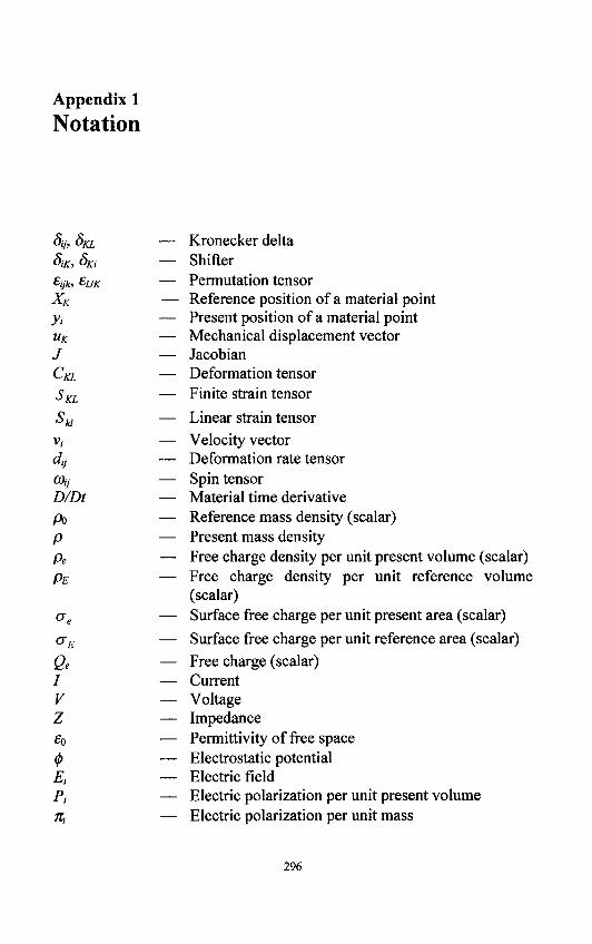
Kronecker delta Shifter Permutation tensor Reference position of a material point Present position of a material point Mechanical displacement vector Jacobian Deformation tensor Finite strain tensor
Linear strain tensor Velocity vector Deformation rate tensor Spin tensor Material time derivative Reference mass density (scalar) Present mass density Free charge density per unit present volume (scalar) Free charge density per unit reference volume (scalar) Surface free charge per unit present area (scalar)
Surface free charge per unit reference area (scalar) Free charge (scalar) Current Voltage Impedance Permittivity of free space Electrostatic potential Electric field Electric polarization per unit present volume Electric polarization per unit mass
296
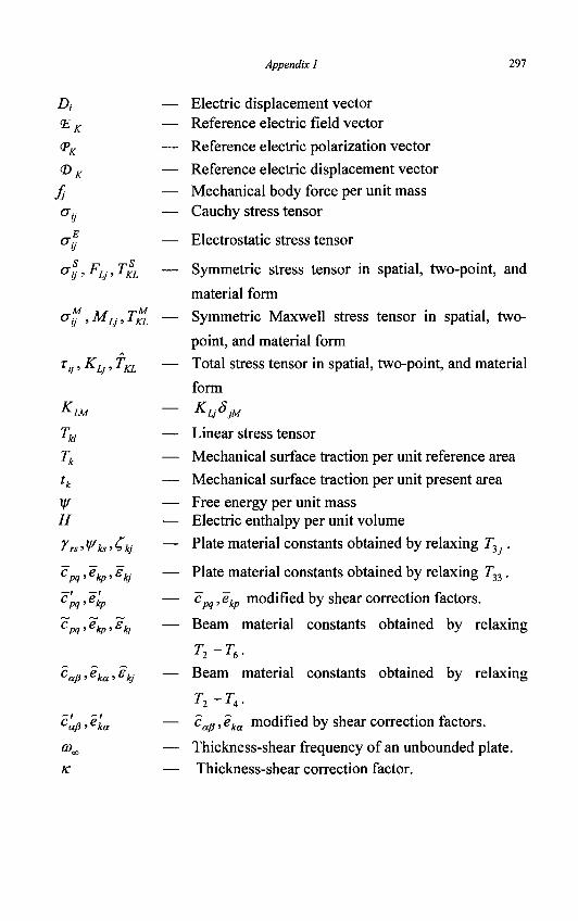
Appendix 1 297
Dt — Electric displacement vector — Reference electric field vector
— Reference electric polarization vector
— Reference electric displacement vector — Mechanical body force per unit mass — Cauchy stress tensor
— Electrostatic stress tensor
— Symmetric stress tensor in spatial, two-point, and
material form
— Symmetric Maxwell stress tensor in spatial, two-
point, and material form
— Total stress tensor in spatial, two-point, and material
form
— KUSJM
— Linear stress tensor
— Mechanical surface traction per unit reference area
— Mechanical surface traction per unit present area
— Free energy per unit mass — Electric enthalpy per unit volume
— Plate material constants obtained by relaxing T3j .
— Plate material constants obtained by relaxing T33.
— ^pq-^kp modified by shear correction factors.
— Beam material constants obtained by relaxing
T2~T6. — Beam material constants obtained by relaxing
T2~T4.
— cap»^ica modified by shear correction factors.
— Thickness-shear frequency of an unbounded plate. — Thickness-shear correction factor.
*K
VK
(DK
fj °V
-1 *!•
<
TV>
Fw-rrrS
<2KL
>MLJJKL
KLj>
KIM
Tu
Tk
h ¥ H
/rs>
Cpq.
c' cpq: Cpq-
Cap
CaP
a* K
Vks,
>ekp'
>ekp
>ekp'
>eka
>eka
TKL
<Qkj
Ekj
£kj
>£kj
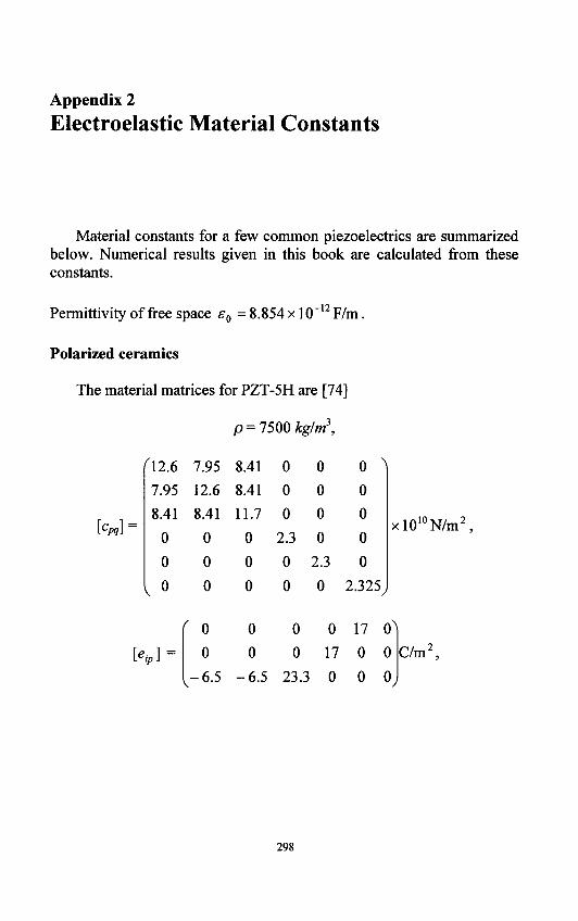
Appendix 2
Electroelastic Material Constants
Material constants for a few common piezoelectrics are summarized below. Numerical results given in this book are calculated from these constants.
Permittivity of free space sQ - 8.854 x 10~12 F/m.
Polarized ceramics
The material matrices for PZT-5H are [74]
p = 7500 kg/m\
Kg]
'12.6
7.95
8.41
0
0
, 0
7.95
12.6
8.41
0
0
0
8.41
8.41
11.7
0
0
0
0
0
0
2.3
0
0
0
0
0
0
2.3
0
0
0
0
0
0
2.325
xl010N/m2 .
KJ 0
0
-6.5
0 0
0 0
-6.5 23.3
0 17 0^
17 0 0
0 0 0,
C/m2,
298
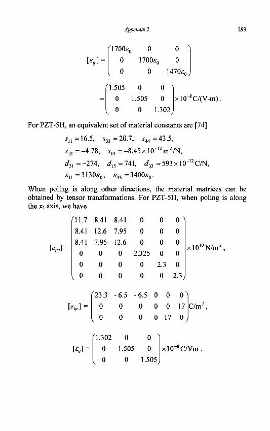
Appendix 2 299
[**] = noos, 0
0
v 0
'1.505
0
0
0
1700ff0
0
0
0
1470f, oy
0
1.505
0
0
0
1.302
xlO"8C/(V-m).
For PZT-5H, an equivalent set of material constants are [74]
•sn=16.5, $33=20.7, $44=43.5,
'12 = -4.78, sl3 = -8.45 x 10~" m'/N,
d3X = -21 A, dl5 = 741, d33 = 593 x 10-12 C/N,
£-,! = 3130f0, E33 = 3400£0.
When poling is along other directions, the material matrices can be obtained by tensor transformations. For PZT-5H, when poling is along the x\ axis, we have
[Cpq] =
'11.7
8.41
8.41
0
0
v 0
K]
8.41 8.41
12.6 7.95
7.95 12.6
0 0
0
0
'23.3
0
0
0
0
•6.5
0
0
0
0
0
2.325
0
0
0
0
0
0
2.3
0
0 ^
0
0
0
0
2.3
xl0 l uN/m'
6.5 0 0 0
0 0 0 17
0 0 17 0
C/m'
[£//] =
'1.302 0
0 1.505
V 0
0
0
0 1.505
xl0~8C/Vm
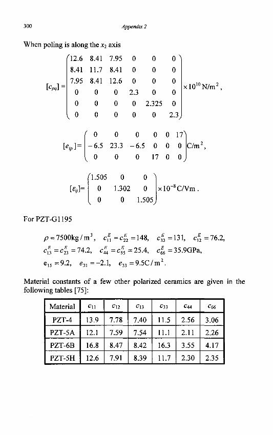
300 Appendix 2
When poling is along the xj axis
M
12.6 8.41
8.41
7.95
0
0
0
11.7
8.41
0
0
0
7.95
8.41
12.6
0
0
0
0
0
0
2.3
0
0
0
0
0
0
2.325
0
0
0
0
0
2.3
\V> xl0 l uN/m J
[**] =
0 0
-6 .5 23.3
0 0
0
-6.5
0
0 0 17N
0 0 0
17 0 0
C/m2,
[%]=
("1.505
0
0
0 0
1.302 0
0 1.505
xlO"8C/Vm
For PZT-G1195
p = 7500kg /m3 E E C\\ = C 22 = 148, '33 : 131, cf2= 76.2,
'23 : 74.2, '44 = 4=25.4, c,
'15 -9 .2 , =31 = -2.1, -33
66-35.9GPa,
= 9.5C/m2.
Material constants of a few other polarized ceramics are given in the following tables [75]:
Material
PZT-4
PZT-5A
PZT-6B
PZT-5H
Cl l
13.9
12.1
16.8
12.6
C12
7.78
7.59
8.47
7.91
Cl3
7.40
7.54
8.42
8.39
C33
11.5
11.1
16.3
11.7
c44
2.56
2.11
3.55
2.30
C66
3.06
2.26
4.17
2.35
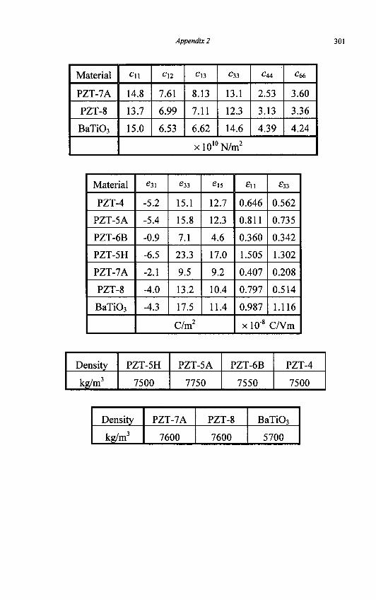
Appendix 2 301
Material
PZT-7A
PZT-8
BaTi03
C\\
14.8
13.7
15.0
Cl2
7.61
6.99
6.53
C\i
8.13
7.11
6.62
C33
13.1
12.3
14.6
c44
2.53
3.13
4.39
C66
3.60
3.36
4.24
xl010N/m2
Material
PZT-4
PZT-5A
PZT-6B
PZT-5H
PZT-7A
PZT-8
BaTi03
C31
-5.2
-5.4
-0.9
-6.5
-2.1
-4.0
-4.3
£33
15.1
15.8
7.1
23.3
9.5
13.2
17.5
e\s
12.7
12.3
4.6
17.0
9.2
10.4
11.4
C/m2
d i
0.646
0.811
0.360
1.505
0.407
0.797
0.987
£33
0.562
0.735
0.342
1.302
0.208
0.514
1.116
x 10"8 C/Vm
Density
kg/m3
PZT-5H
7500
PZT-5A
7750
PZT-6B
7550
PZT-4
7500
Density
kg/m3
PZT-7A
7600
PZT-8
7600
BaTi03
5700
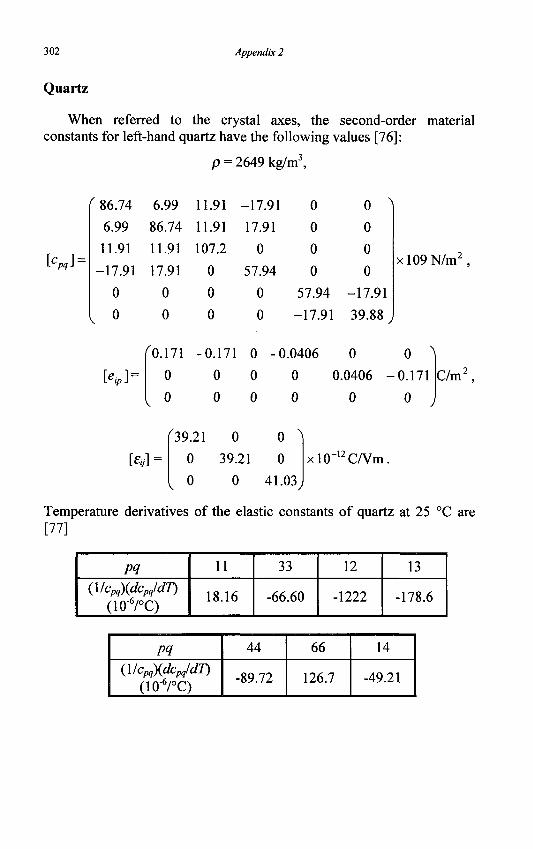
302 Appendix 2
Quartz
When referred to the crystal axes, the second-order material constants for left-hand quartz have the following values [76]:
p = 2649 kg/m3,
['«] = m
( 86.74
6.99
11.91
-17.91
0
0
6.99
86.74
11.91
17.91
0
0
11.91
11.91
107.2
0
0
0
-17.91
17.91
0
57.94
0
0
0
0
0
0
57.94
-17.91
0
0
0
0
-17.91
39.88
xl09N/m2
[*»] =
'0.171 -0.171 0
0 0 0
0 0 0
0.0406 0 0 "
0 0.0406 -0.171 C/m2
0 0 0 ,
w = 39.21 0
0
0
0
39.21 0
0 41.03
xl0~"C/Vm.
Temperature derivatives of the elastic constants of quartz at 25 °C are [77]
pq {\lcpq){dcpqldT)
(10-6/°C)
11
18.16
33
-66.60
12
-1222
13
-178.6
M (\lcpq)(dcpqldT)
(10-6/°C)
44
-89.72
66
126.7
14
-49.21
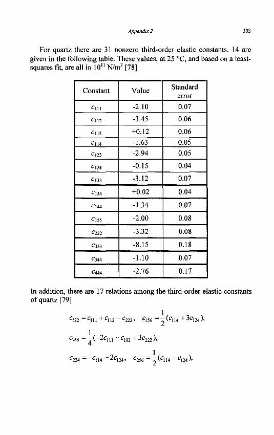
Appendix 2 303
For quartz there are 31 nonzero third-order elastic constants. 14 are given in the following table. These values, at 25 °C, and based on a least-squares fit, are all in 10u N/m2 [78]
Constant
C m
Cm
ClB
Cll4
Cl23
Cm
Cm
Cl34
C144
Cl55
cm
C333
C344
C444
Value
-2.10
-3.45
+0.12
-1.63
-2.94
-0.15
-3.12
+0.02
-1.34
-2.00
-3.32
-8.15
-1.10
-2.76
Standard error
0.07
0.06
0.06
0.05
0.05
0.04
0.07
0.04
0.07
0.08
0.08
0.18
0.07
0.17
In addition, there are 17 relations among the third-order elastic constants of quartz [79]
_ 1
C122 _ C 111 + C112 C222' C156- (ClH+3CUii),
C166 ~ T ( — 2 C n , — C H 2 +3c222h
C224 = ~C\ 14 _ ^C124, C256 = —(Cj 14 - C124 ) ,
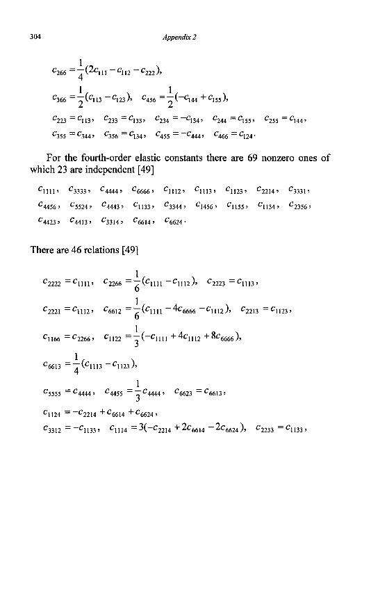
304 Appendix 2
C266 ~ S^C\\\ C\ 12 C222)>
C366 _ ~VC113 C 1 2 3 / ' C456 ~ ~\ C144 + C155.)>
C 2 2 3 = C 1 1 3 > C 2 3 3 = C 1 3 3 > C 2 3 4 = _ C 1 3 4 > C 2 4 4 ~ C 1 5 5 ' C 2 5 5 = C 1 4 4 >
C355 ~ C 3 4 4 ' C 3 5 6 = C 1 3 4 > C 4 5 5 = _ C 4 4 4 > C 4 6 6 ~ C 1 2 4 -
For the fourth-order elastic constants there are 69 nonzero ones of which 23 are independent [49]
C 1 1 U ' C3333> C4444> C 6 6 6 6 ' C 1112 ' C1113> C 1 1 2 3 ' C 2 2 1 4 ' C3331»
C 4 4 5 6 ' C5524> C4443 > C 1133 ' C3344 > C1456 > C 1 1 5 5 ' C1134> C 2 3 5 6 '
C4423> C4413> C 3 3 1 4 ' C6614 > C6624 •
There are 46 relations [49]
C2222 _ C 1 1 1 1 > C2266 _ , VC1111 c \ m h C 2 2 2 3 _ C 1 1 1 3 '
C2221 = C 1 1 1 2 ' C6612 = T ( C 1 1 1 1 _ 4 C 6 6 6 6 - C 1 1 1 2 ) , C 2 2 1 3 = C 1 1 2 3 , O
C1166 = C2266> C1122 = TT ( — C l 111 + 4C1112 + °C6666 )»
_ 1 , _ x C6613 - . VC1113 C1123 J»
_1 C5555 _ C4444 ' C4455 _ - C4444 » C6623 ~~ C6613 >
C1124 - _ C 2 2 1 4 + C6614 + C6624 '
C3312 = _ C 1 1 3 3 » C1114 = A _ C 2 2 1 4 +^C66U _ ^ C 6 6 2 4 ) , C 2 2 3 3 = C 1 1 3 3 ,
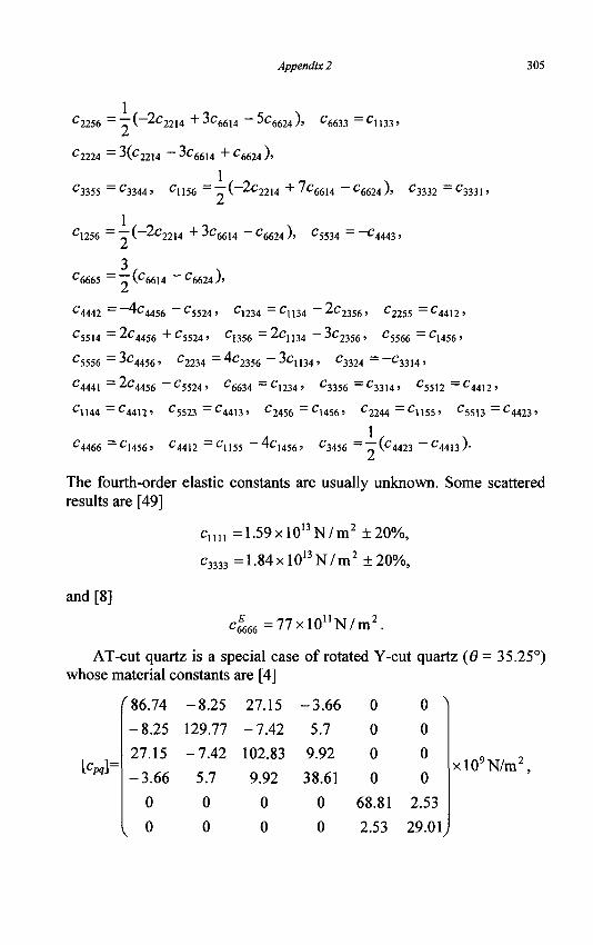
Appendix 2 305
2256 — „ ( 2C2 2i4 + 3 C 6 6 1 4 5C 6 6 2 4 ) , Cfi633 — C U 3 3 , c
C2224 -AC2214 "" ' 6614 + C, 6624 )'
C3355 - C 3344' '1156 2 : „ ( 2c2214 + 7c6 6 H c6624), '3332 ' 3 3 3 1 '
'1256 _ « ( 2 c 2 2 1 4 + 3C 6 6 1 4 C6 6 2 4 ) , C5 5 3 4 --C
C6665 _ „ (C6614 C6624 )>
4442 ~ ^ C 4456
5514 — 2 C 4 4 5 6 + C 5 5 2 4 ,
C5524» C1234 _ C 1 1 3 4
C
-2c 2356'
4443'
'2255 = C 4412'
1356 - 2 C U 3 4 3 C 2 3 5 6 , C5566 ~ C 1456'
5556 - 3 C 4 4 5 6 , C2234 _ 4 C 2 3 5 6 3C, 134' C3324 _ C 3314'
c4441 _ 2 C 4 4 5 6
'1144 ' 4 4 1 2 '
' 5524 '
'5523
'6634
' 4 4 1 3 '
'1234 '
'2456
'3356
'1456 '
" ^ 3 3 1 4 ' '5512
'2244 1155'
" ' ' 4 4 1 2 '
'5513 4423'
C4466 ~C 1456' '4412 = C, 155 4 ^ 1 4 5 6 ' C3456 _ - (C4423 C4413 )•
The fourth-order elastic constants are usually unknown. Some scattered results are [49]
' m i = 1.59xl01 3N/m2+20%,
c3333 =1.84xl01 3N/m2 ±20%,
and [8]
'6666 : 77x lO n N/m 2 .
AT-cut quartz is a special case of rotated Y-cut quartz (G = 35.25°) whose material constants are [4]
^86.74 -8.25 27.15
-8.25 129.77 -7.42
27.15 -7.42 102.83
-3.66 5.7 9.92
0 0 0
0 0 0
[c„]=
-3.66
5.7
9.92
38.61
0
0
0
0
0
0
68.81
2.53
0 N
0
0
0
2.53
29.01;
xl09N/m2
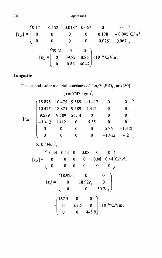
306 Appendix 2
K] 171 -0.152 •
0 0
0 0
[«*] =
'39.21
0
, o
•0.0187
0
0
0
39.82
0.86
0.067 0 0
0 0.108 -0.095
0 -0.0761 0.067
0 ^
0.86
40.42
xlO-12C/Vm.
C/m'
Langasite
The second-order material constants of La3Ga5SiOi4 are [80]
p = 5743 kg/m3,
10.475 9.589 -1.412 0 0
18.875 9.589 1.412 0 0
9.589 26.14 0 0 0
1.412 0 5.35 0 0
0 0 0 5.35 -1.412
0 0 0 -1.412 4.2
[Cpq]
O 8.875
10.475
9.589
-1.412
0
0
\
V
xl010N/m2
J
K]= .0.44 0.44 0
0
0
[<%] =
0
0
18.92^
0
0
o
v
067.5
0
V 0
-0.08
0
0
0
18.92f0
0
0 0 A
0.08 0.44
0 0
0
0
50.7s,
C/nV
oy
0 0
167.5 0
0 448.9
xlO~12C/Vm.
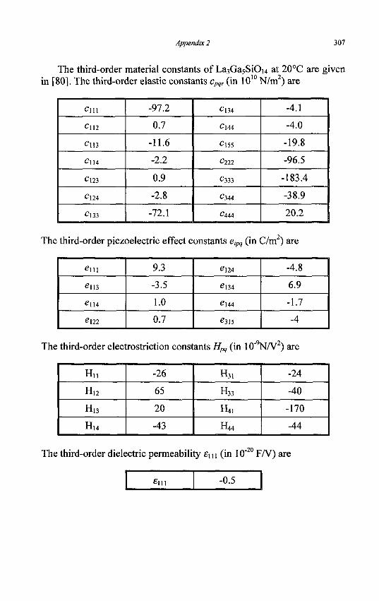
Appendix 2 307
The third-order material constants of La3Ga5SiOi4 at 20°C are given in [80]. The third-order elastic constants cpqr (in 1010 N/m2) are
C\\\
Cm
C\U
Cll4
cm
C\U
cm
-97.2
0.7
-11.6
-2.2
0.9
-2.8
-72.1
Cl34
Cj44
Cl55
C222
C333
C344
C444
-4.1
-4.0
-19.8
-96.5
-183.4
-38.9
20.2
The third-order piezoelectric effect constants eipq (in C/m2) are
em
em
e\u
^122
9.3 I e124
-3.5
1.0
0.7
^134
e i44
^315
-4.8
6.9
-1.7
-4
The third-order electrostriction constants Hpq (in lO'^/V2) are
H„ H,2
HI3
H14
-26
65
20
-43
H31
H33
H41
H44
-24
-40
-170
-44
The third-order dielectric permeability em (in 10" F/V) are
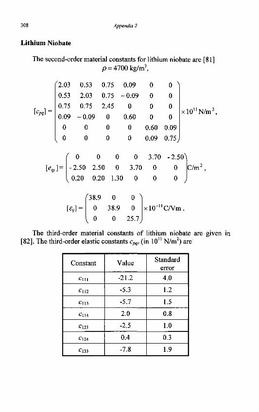
308 Appendix 2
Lithium Niobate
The second-order material constants for lithium niobate are [81] p = 4700kg/m3,
'2.03
0.53
M =
0.53
2.03
0.75 0.75
0.09 -0.09
0
0
KY-
0
0
0.75
0.75
2.45
0
0
0
0.09
-0.09
0
0.60
0
0
f 0 0
2.50 2.50 (
V
0
0
0.20 0.20 1.30
0
0
0
0
0 ^
0
0
0
0.60 0.09
0.09 0.75
x l0 u N/m :
0 3.70
3.70 0
0 0
J
• 2.50^
0
0 j
C/m'
[£(,]
'38.9 0
0 38.9
\
0 0
0
0
25.7
xl0-uC/Vm
The third-order material constants of lithium niobate are given in [82]. The third-order elastic constants cpqr (in 10u N/m2) are
Constant
Cm
Cm
Cl l3
Cl l4
cm
C\24
cm
Value
-21.2
-5.3
-5.7
2.0
-2.5
0.4
-7.8
Standard error
4.0
1.2
1.5
0.8
1.0
0.3
1.9
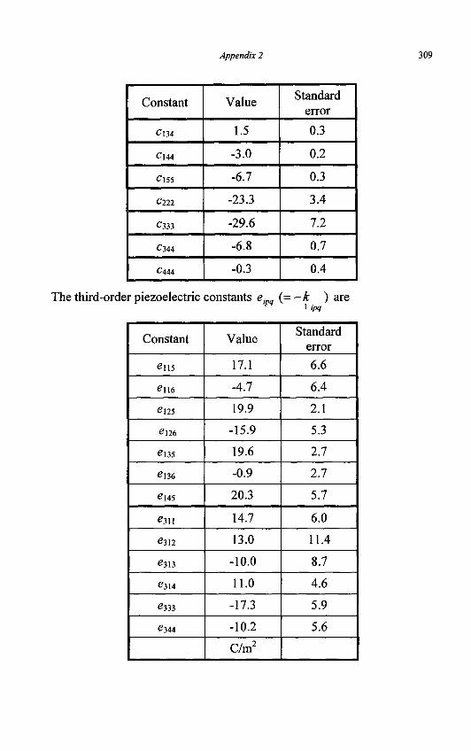
Appendix 2 309
Constant
Cm
C144
Cl55
Cm
cm
C344
C444
Value
1.5
-3.0
-6.7
-23.3
-29.6
-6.8
-0.3
Standard error
0.3
0.2
0.3
3.4
7.2
0.7
0.4
The third-order piezoelectric constants e( (=-k ) are 1 ipq
Constant
ens
e\\6
C\2%
C\2(,
£135
e i36
^145
^311
^312
^313
^314
<?333
^344
Value
17.1
-4.7
19.9
-15.9
19.6
-0.9
20.3
14.7
13.0
-10.0
11.0
-17.3
-10.2
C/m2
Standard error
6.6
6.4
2.1
5.3
2.7
2.7
5.7
6.0
11.4
8.7
4.6
5.9
5.6
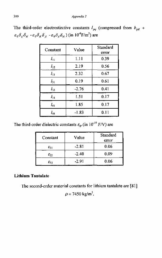
310 Appendix 2
The third-order electrostirctive constants lpq (compressed from bijkl +
£odij$ki -£<>SikSji -s0S,,Skl)(mW9F/m2)are
Constant
hi
hi
In
hi
hi
hn
hi
hn
Value
1.11
2.19
2.32
0.19
-2.76
1.51
1.85
-1.83
Standard error
0.39
0.56
0.67
0.61
0.41
0.17
0.17
0.11
The third-order dielectric constants eip (in 10" F/V) are
Constant
£31
1 £22
£33
Value
-2.81
-2.40
-2.91
Standard error
0.06
0.09
0.06
Lithium Tantalate
The second-order material constants for lithium tantalate are [81]
p = 7450kg/m3,
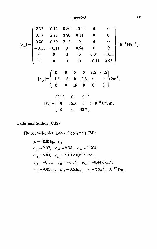
Appendix 2
[Cpq]
f 2.33
0.47
0.80
-0.11
0
0
0.47
2.33
0.80
-0.11
0
0
0.80
0.80
2.45
0
0
0
-0.11
0.11
0
0.94
0
0
0
0
0
0
0.94
-0.11
0
0
0
0
-0.11
0.93
xlO1
KJ =
f 0 0 0 0 2.6 -1.6A
1.6 1.6 0 2.6 0 0
0 0 1.9 0 0 0
C/m2,
[%]
V
36.3 0 0 ^
0 36.3 0
0 0 38.2y
xlO_uC/Vm.
Cadmium Sulfide (CdS)
The second-order material constants [74]:
/> = 4820kg/m3,
c n =9.07 , c33=9.38, c44 =1.504,
c,2=5.81, c1 3=5.10xl01 0N/m2 ,
-0.21, = 31 -0.24, e3 3=-0.44 C/m3
su =9.02£0, £33 =9.53^0, e0 =8.854 xl0~12F/m.
Index
actuator 122, 133,150, 207 antiresonance 58 apparent material constant 16 beam 225 Bessel function 56, 221 bias 12, 168 bimorph 172, 249 Bleustein-Gulyaev wave 33, 167 boundary element 157, 206 boundary integral equation 206 buckling 172 cadmium sulfide 86, 311 capacitance 28, 104, 278, 287 Cauchy 34 ceramic 32, 49, 72, 78, 82, 91, 172, 201,
231,234,249,268,298 charge 10, 57 charge equation 3 circuit condition 10, 94, 255, 277, 286 classical flexure 66, 130, 133, 196, 242,
266 Coriolis 93, 275 correction factor 37, 61, 78, 96, 183,
239 cubic 19, 179 current 10, 57 cutoff frequency 33 cylindrical coordinates 203, 218, 262 damping coefficient 186 degeneracy 116 Dirac delta function 153 dispersion relation 33, 48, 66, 115, 117,
118,121,132,166,222,224 double resonance 95 effective material constant 16 efficiency 289 eigenvalue problem 104,235, 255 electromechanical coupling factor 175,
278 energy trapping 88, 120
enthalpy 8 extension 33,47, 228 face-shear 33, 47 finite difference 159 finite element 142 first-order theory 58, 127, 147, 168,
180, 189,235,262 flexure
classical (see classical flexure) shear deformation 64,132
forced vibration 27, 185, 280, 283 four-vector213 free energy 3, 7, 18,20 free vibration 25, 82, 104, 185, 201,
235, 252, 268, 277 frequency split 279 Gauss's equation 3 gyroscope 91, 274 half-space 150 harmonic 235 initial fields (see bias) initial stress theory 18, 172 integral-differential equation 152, 206 isotropic 64, 68, 70,112, 135 Kane-Mindlin theory 111 Kirchhoff34, 36 Kronecker delta 1, 2 Lam6 coefficient 190 Lame constant 64,112 laminate 145 langasite 22, 306 lithium niobate 308 lithium tantalate 310 Love wave 167 matrix notation 11 membrane theory 199, 204, 211 Mindlin-Medick theory 111 monoclinic crystal 23, 98 motional capacitance 104 nonlinear 1, 19, 168
312
Index 313
non-slip condition 222 orthogonality 107 overtone 235 parallelepiped 270 permittivity 3, 298 perturbation 214 piezoelectric stiffening 86, 279 plate 22 Poisson 34 Poisson's effect 41, 58, 236 Poisson's ratio 65, 142 polar coordinates 55, 140, 217 positive-definite 8 potential 3 quality factor 186, 280, 288 quartz 22, 96, 102, 184,302 Rayleigh
quotient 107, 220 wave 33
relaxed material constants for plates 45, 46, 182
resonance 26, 57 resonator 102 ring 217, 262 Rosen transformer 289 saturation 282, 289 second-order theory 107 self-adjoint 107 sensor
angular rate 91, 274 fluid 220 mass 210
shell 189 shifter 2 spherical coordinates 201 strain
finite 4 infinitesimal 9
stress concentration 154 stress function 138 stress relaxation 44, 46, 62, 96, 110,
170, 182,229,237,246
substrate 150 surface wave 162 thickness-shear
approximation 69, 74, 244 correction factor 78, 96, 183, 239 nonlinear 179 static deformation 27 vibration 22, 184 wave 33
thickness-stretch approximation 117 deformation 111 wave 33
thickness-twist 33 torsion 220 transformer 252, 283 transverse isotropy 32 unimorph 133 variation5, 11, 16, 107 vibration
beam 234 circular disk 54 cylindrical shell 202 ring 268 spherical shell 201
viscosity 221 wave
extension 33,47 face-shear 33, 47 flexure 33, 64 high-frequency 33 low-frequency 33 straight-crested 29, 113 surface 33,162 thickness-shear 33, 64, 132 thickness-stretch 33, 115, 117, 118 thickness-twist 33 torsional 220
width-shear 235 zero-order theory 41, 228, 273
The Mechanics of Piezoelectric Structures
A continuation of the author's previous book "An Introduction
to the Theory of Piezoelectricity" (Springer, New York, 2005)
on the three-dimensional theory of piezoelectricity, this volume
covers lower dimensional theories for various piezoelectric structures
and device applications. The development of two-, one- and zero-
dimensional theories for high frequency vibrations of piezoelectric
plates, shells, beams, rings and parallelepipeds is systematically
presented. In addition to linear piezoelectricity, certain nonlinear
effects are also considered and examples for device applications
are provided.
The material emphasizes dynamic theories and high frequency
motions as well as device applications as there are relatively few
books on piezoelectric structures, especially for high frequency
theories. The volume is destined to be one of the most systematic
and comprehensive books on piezoelectric structures.
v;J 'orld Scientific
YEARS OF PUftl ISHIN< 1 - 2 0 0 1
9 "789812 5670171
v.worldscientific.com