Embed Size (px)
Citation preview

The Material Point Method for SimulatingContinuum Materials
Chenfanfu Jiang∗1, Craig Schroeder†2, Joseph Teran‡1,3,Alexey Stomakhin§3, and Andrew Selle¶3
1Department of Mathematics, University of California, Los Angeles2Department of Computer Science, University of California, Riverside
3Walt Disney Animation Studios
SIGGRAPH 2016 Course Notes Version 1 (May 2016)
Permission to make digital or hard copies of part or all of this work for personal orclassroom use is granted without fee provided that copies are not made or distributedfor profit or commercial advantage and that copies bear this notice and the full cita-tion on the first page. Copyrights for third-party components of this work must behonored. For all other uses, contact the Owner/Author. Copyright is held by the own-er/author(s).SIGGRAPH ’16 Courses, July 24-28, 2016, Anaheim, CA,ACM 978-1-4503-4289-6/16/07.http://dx.doi.org/10.1145/2897826.2927348
∗ [email protected]† [email protected]‡ [email protected]§ [email protected]¶ [email protected]
1

2
abstract
Simulating the physical behaviors of deformable objects and fluids has been an impor-tant topic in computer graphics. While the Lagrangian Finite Element Method (FEM) iswidely used for elasto-plastic solids, it usually requires additional computational compo-nents in the case of large deformation, mesh distortion, fracture, self-collision and cou-pling between materials. Often, special solvers and strategies need to be developed fora particular problem. Recently, the hybrid Eulerian/Lagrangian Material Point Method(MPM) was introduced to the graphics community. It uses a continuum description ofthe governing equations and utilizes user-controllable elasto-plastic constitutive models.The hybrid nature of MPM allows using a regular Cartesian grid to automate treatmentof self-collision and fracture. Like other particle methods such as Smoothed ParticleHydrodynamics (SPH), topology change is easy due to the lack of explicit connectivitybetween Lagrangian particles. Furthermore, MPM allows a grid-based implicit integra-tion scheme that has conditioning independent of the number of Lagrangian particles.MPM also provides a unified particle simulation framework similar to Position BasedDynamics (PBD) for easy coupling of different materials. The power of MPM has beendemonstrated in a number of recent papers for simulating various materials includingelastic objects, snow, lava, sand and viscoelastic fluids. It is also highly integrated into theproduction framework of Walt Disney Animation Studios and has been used in featuredanimations including Frozen, Big Hero 6 and Zootopia.
Contents 3
contents1 About the Lecturers 5
2 Syllabus 7
2.1 Intended Audience . . . . . . . . . . . . . . . . . . . . . . . . . . . . . . . . . 7
2.2 Prerequisites . . . . . . . . . . . . . . . . . . . . . . . . . . . . . . . . . . . . . 7
2.3 Level of Difficulty . . . . . . . . . . . . . . . . . . . . . . . . . . . . . . . . . . 7
2.4 Tentative Schedule . . . . . . . . . . . . . . . . . . . . . . . . . . . . . . . . . 7
3 Introduction 9
4 MPM in Production 10
5 Kinematics Theory 10
5.1 Continuum Motion . . . . . . . . . . . . . . . . . . . . . . . . . . . . . . . . . 11
5.2 Deformation . . . . . . . . . . . . . . . . . . . . . . . . . . . . . . . . . . . . . 12
5.3 Push Forward and Pull Back . . . . . . . . . . . . . . . . . . . . . . . . . . . . 13
5.4 Material Derivative . . . . . . . . . . . . . . . . . . . . . . . . . . . . . . . . . 15
5.5 Volume and Area Change . . . . . . . . . . . . . . . . . . . . . . . . . . . . . 16
6 Hyperelasticity 17
6.1 First Piola-Kirchoff Stress . . . . . . . . . . . . . . . . . . . . . . . . . . . . . 18
6.2 Neo-Hookean . . . . . . . . . . . . . . . . . . . . . . . . . . . . . . . . . . . . 19
6.3 Fixed Corotated Constitutive Model . . . . . . . . . . . . . . . . . . . . . . . 19
6.4 A Practical Differentiation Strategy for Isotropic Elasticity . . . . . . . . . . 21
6.5 Snow Plasticity . . . . . . . . . . . . . . . . . . . . . . . . . . . . . . . . . . . 25
7 Governing Equations 27
7.1 Conservation of Mass . . . . . . . . . . . . . . . . . . . . . . . . . . . . . . . . 28
7.2 Conservation of Momentum . . . . . . . . . . . . . . . . . . . . . . . . . . . . 29
7.3 Weak Form . . . . . . . . . . . . . . . . . . . . . . . . . . . . . . . . . . . . . . 30
8 Material Particles 31
8.1 Eulerian Interpolating Functions . . . . . . . . . . . . . . . . . . . . . . . . . 32
8.2 Eulerian/Lagrangian Mass . . . . . . . . . . . . . . . . . . . . . . . . . . . . . 33
8.3 Eulerian/Lagrangian Momentum . . . . . . . . . . . . . . . . . . . . . . . . . 34
8.4 Eulerian to Lagrangian Transfer . . . . . . . . . . . . . . . . . . . . . . . . . . 35
9 Discretization 35
9.1 Discrete Time . . . . . . . . . . . . . . . . . . . . . . . . . . . . . . . . . . . . 35
9.2 Discrete Space . . . . . . . . . . . . . . . . . . . . . . . . . . . . . . . . . . . . 36
9.3 Estimating the Volume . . . . . . . . . . . . . . . . . . . . . . . . . . . . . . . 38
9.4 Deformation Gradient Evolution . . . . . . . . . . . . . . . . . . . . . . . . . 38
9.5 Forces as Energy Gradient . . . . . . . . . . . . . . . . . . . . . . . . . . . . . 39
10 Explicit Time Integration 41
10.1 APIC Transfers . . . . . . . . . . . . . . . . . . . . . . . . . . . . . . . . . . . . 41
10.2 Deformation Gradient Update . . . . . . . . . . . . . . . . . . . . . . . . . . . 42
10.3 State Update . . . . . . . . . . . . . . . . . . . . . . . . . . . . . . . . . . . . . 43
10.4 Forces . . . . . . . . . . . . . . . . . . . . . . . . . . . . . . . . . . . . . . . . . 43

Contents 4
10.5 MPM Scheme: Full Algorithm . . . . . . . . . . . . . . . . . . . . . . . . . . . 44
11 Implicit Time Integration 45
11.1 Force Derivative . . . . . . . . . . . . . . . . . . . . . . . . . . . . . . . . . . . 45
11.2 Backward Euler System . . . . . . . . . . . . . . . . . . . . . . . . . . . . . . 46
11.3 Newton’s Method . . . . . . . . . . . . . . . . . . . . . . . . . . . . . . . . . . 47
11.4 Linearized Force . . . . . . . . . . . . . . . . . . . . . . . . . . . . . . . . . . . 47
11.5 Optimization based Integrator . . . . . . . . . . . . . . . . . . . . . . . . . . . 48
12 More Topics 49
12.1 Collision Objects . . . . . . . . . . . . . . . . . . . . . . . . . . . . . . . . . . . 49
12.2 Lagrangian Forces . . . . . . . . . . . . . . . . . . . . . . . . . . . . . . . . . . 50
Bibliography 51

about the lecturers 5
1 about the lecturers
Chenfanfu JiangMathematics DepartmentUniversity of California, Los [email protected]
Chenfanfu Jiang received his Ph.D. in Computer Science at UCLA in 2015, awardedUCLA Engineering School Edward K. Rice Outstanding Doctoral Student. He is currentlya postdoctoral researcher at UCLA, jointly appointed to the departments of Mathematicsand Computer Science. His primary research interests include solid/fluid mechanics,physics based simulation and their applications to medical simulation and scene under-standing. He actively collaborates with Walt Disney Animation Studios and Center forAdvanced Surgical and Interventional Technology (CASIT).
Craig SchroederComputer Science DepartmentUniversity of California, [email protected]
Craig Schroeder is currently an assistant professor in computer science at University ofCalifornia Riverside. He received his Ph.D. in computer science from Stanford Universityin 2011, followed by a postdoc at University of California Los Angeles, where he receivedthe Chancellor’s Award for Postdoctoral Research in 2013, recognizing research impactand value to the UCLA community. He actively publishes in both computer graphics andcomputational physics. His primary areas of interest are solid mechanics and computa-tional fluid dynamics and their applications to physically based animation for computergraphics. He began collaborating with Pixar Animation Studios during his Ph.D. andlater collaborated with Walt Disney Animation Studios during his postdoctoral studies.For his research contributions he received screen credits in Pixar’s "Up" and Disney’s"Frozen."
Joseph TeranMathematics DepartmentUniversity of California, Los [email protected]
about the lecturers 6
Joseph Teran is a professor of applied mathematics at UCLA. His research focuses onnumerical methods for partial differential equations in classical physics, including com-putational solids and fluids, multi-material interactions, fracture dynamics and compu-tational biomechanics. He also works with Walt Disney Animation applying scientificcomputing techniques to simulate the dynamics of virtual materials like skin/soft tissue,water, smoke and recently, snow for the movie “Frozen". Teran received a 2011 Presi-dential Early Career Award for Scientists and Engineers (PECASE) and a 2010 YoungInvestigator award from the Office of Naval Research.
Alexey StomakhinWalt Disney Animation [email protected]
Alexey Stomakhin is a Senior Software Engineer at Walt Disney Animation Studios. Heis responsible for developing tools for simulation of environmental effects. He is thelead developer of the Disney in-house Material Point Method engine (a.k.a. Matterhorn)which was used extensively for snow simulation in Frozen (2013), and also in Big Hero 6
(2014) and Zootopia (2016). He also does research and works extensively on the simula-tion of fluids, multi-material interactions and parallel/distributed computing. He holdsa Ph.D. degree in Mathematics from University of California, Los Angeles (2013).
Andrew SelleWalt Disney Animation [email protected]
Andrew Selle, Principal Software Engineer, is responsible for developing tools and tech-niques for simulation and rendering at Walt Disney Animation Studios. He focusedon fluid simulation techniques in "Tangled", rigid bodies and volumetric rendering on"Wreck-It-Ralph" and Snow simulation and rendering on "Frozen." He also was a majordeveloper on Disney’s Hyperion Renderer used in Big Hero 6, Feast, Zootopia, and allupcoming Disney Animation Films. As part of his work he has contributed to the opensource community by releasing and maintaining the SeExpr and Partio libraries. Besidesdevelopment, he remains active in research oriented publication, continuing to publisharticles in refereed journals and conferences. Prior to his current position, he was a Re-search and Development Software Engineer at Industrial Light + Magic. He holds a B.S.in Mathematics in Computer Science from the University of Wisconsin Madison and aM.S. and Ph.D. in Computer Science from Stanford University.

syllabus 7
2 syllabus
2.1 Intended Audience
These notes are intended for industry professionals and academic researchers interestedin recent advances in the Material Point Method for simulating various materials forcomputer animation and visual effects.
2.2 Prerequisites
This course requires minimal concepts of continuum mechanics. Familiarity with mul-tivariable calculus, linear algebra and common numerical algorithms is assumed. Noexperience of MPM is required. Some previous knowledge and experience with theFinite Element Method (FEM) and continuum mechanics would benefit.
2.3 Level of Difficulty
Easy/Intermediate.
2.4 Tentative Schedule
1. Introduction and Welcome (All speakers) (5 min)
• Introduction of Speakers
• Course overview
• MPM introduction: advantages and limitations
• Research demos, Disney production clips
2. MPM in Disney (Alexey Stomakhin, Andrew Selle) (35 min)
3. Continuum Mechanics Concepts (Joseph Teran) (15 min)
• Continuum description of material motion
• Kinematics, deformation gradient, strain
• Stress and hyperelasticity
• Governing equations, conservation of mass/momentum
4. MPM Algorithm (Explicit integration) (Chenfanfu Jiang) (15 min)
• Particle-Grid transfers

syllabus 8
• Deformation gradient update
• Force computations
• Symplectic Euler time integration
• The full MPM algorithm
5. MPM Algorithm (Implicit integration) (Craig Schroeder) (15 min)
• Force derivative computations
• Backward Euler time integration
• Force linearization
• Newton’s method for MPM
6. Conclusion (Joseph Teran) (5 min)
• Difficulties and workarounds
• Open problems, interesting research directions
• Conclusion, Q&A

introduction 9
3 introduction
Simulating natural phenomena for virtual worlds and characters is an important appli-cation that remains extremely challenging. An artist’s need to manipulate and compre-hend physical simulations imposes a significant constraint, all but requiring simulationmethods to involve Lagrangian particles. In addition, the need for computational ef-ficiency, topology change and numerical stability has led engineers toward hybrid La-grangian/Eulerian methods. In this course, we focus on the Material Point Method(MPM), which rises as the generalization of Particle In Cell (PIC) and Fluid Implicit Par-ticle Method (FLIP) to solid mechanics [Sulsky et al., 1995]. MPM methods combineLagrangian material particles (points) with Eulerian Cartesian grids. Notably, there is noinherent need for Lagrangian mesh connectivity.
Many researchers in graphics have experimented with hybrid grid and particle methods.While FLIP has been known in graphics community as a useful liquid simulation methodfor a while [Zhu and Bridson, 2005; Bridson, 2008; Ando and Tsuruno, 2011], MPM is onlyintroduced and studied recently.
MPM has been shown to be a very effective hybrid particle/grid method for simulatingvarious solid materials in computer graphics. Stomakhin et al. [2013] and Disney’s Frozenuse MPM to simulate snow. Hegemann et al. [2013] uses impulses derived from MPM toresolve colliding embedded deformable object pieces. Stomakhin et al. [2014] augmentsMPM for simulating incompressible materials and melting/freezing. Ram et al. [2015]and Yue et al. [2015] show that MPM is also suitable for complex fluids. Gast et al. [2015]presents an optimization based integrator to accelerate the nonlinear MPM solver. Jianget al. [2015]; Jiang [2015]; Jiang et al. [2016] propose a stable and angular momentumconserving scheme to improve the particle/grid transfers in MPM. Klar et al. [2016] andDaviet and Bertails-Descoubes [2016] use MPM to discretize the engineering favoredDrucker-Prager elastoplastity to simulate sand dynamics.
As with PIC/FLIP, MPM implicitly handles self-collision and fracture with the use ofthe background Eulerian grid. As a hybrid Lagrangian/Eulerian approach, MPM hasthe following advantages when compared with traditional Lagrangian methods (such asFEM solids) and Eulerian methods (such as grid-based fluids):
• Just like Lagrangian FEM, MPM can be derived from the weak form of conservationof momentum, allowing for physically accurate discretization of physical laws.• Boundary conditions, solid wall collisions and external forces can be easily applied
on the grid and particles.• Automatic self collision/contact due to the fact that particle movements are inter-
polated from undistortable nodal movement on a grid.• Automatic splitting and merging behaviors because of particle based material rep-
resentation. This is remarkably useful for fluids and granular materials.

mpm in production 10
• Automatic multi-material and multiphase coupling can be easily done solely bygiving particles different material properties or constitutive models.• MPM can also be used to simulate mesh-based Lagrangian forces without loosing
its advantages. (See Section 12.2.) This provides the opportunity of coupling pointbased objects and mesh based objects with a single solve on the grid that handlescollisions automatically.
More rigorously speaking, MPM is a Lagrangian method, but with an Eulerian gridused for computing derivatives. This alleviates the need for a Lagrangian mesh (forderivative computation) that would get tangled when the material is highly deformedfrom its original configuration. This lets you simulate a wider class of materials thanwith a purely Lagrangian method. The Eulerian aspects allow for natural treatment oftopological changes and collisions (self and with external objects). There is a sacrifice ofsome accuracy in doing this though and materials like e.g. hyperelasticity are not goingto be simulated as effectively. On the other hand, you get self collisions and topologychanges for free.
4 mpm in production
MPM is adopted in Walt Disney Animation Studios for simulating various materialsincluding most of the dynamic snow in Frozen. It is also highly integrated into theproduction framework of Big Hero 6 and Zootopia.
5 kinematics theory
The contents in this section mostly follow [Bonet and Wood, 2008]. We summarize theimportant concepts that are helpful for understanding the essence of MPM.
First and foremost, MPM particles are not individual particles, molecules, atoms or littlespheres as one may naturally think when seeing a “particle” method. Each MPM par-ticle actually represents a continuous piece of material, or really a subset of the wholesimulated material domain. For those familiar with FEM style weak forms of equations,material points can be thought of as quadrature points for the discretization of spatialstress derivatives (we will talk about the discretization in Section 9).
Such a view is very common in computational mechanics. When we talk about contin-uum bodies or continuum mechanics, we have adopted the continuum assumption. Thismeans the studied material (either solid, liquid or gas) is treated as continuous pieces ofmatter. Such a view is very practical in engineering and graphics applications (as wellas in everyday life) where it is really not necessary to deal with the microscopic inter-

kinematics theory 11
actions between molecules and atoms. Note that a continuum assumption can be madefor almost all solids and fluids that are extensively simulated for graphics, including de-formable (elastic and plastic) objects, muscle, flesh, cloth, hair, liquids, smoke, gas andgranular materials (sand, snow, mud, soil etc.). A continuum body defines quantitiessuch as density, velocity, and force as continuous functions of position. Equations ofmotion are solved in the spatial domain, and evolved in time to simulate the behaviorsof the simulated materials.
5.1 Continuum Motion
Kinematics refers to the study of motion occurred in continuum materials. The mainfocus is the change of shape, or the deformation, either locally or globally in differentcoordinate systems of interest. Describing the motion qualitatively and quantitatively isvery essential for deriving governing equations of dynamics and mechanical responses.Luckily in most cases, we can describe kinematics without introducing the meaning offorce, stress or even mass.
In continuum mechanics, the deformation is usually represented with the material (orundeformed) space X, the world (or deformed) space x and a deformation map φ(X, t).You can simply treat X as the “initial position” and x as the “current position” for anypoint in the simulated material. In particular, at time t = 0, X and x have the same value.
Here is a more detailed definition. We consider the motion of material to be determinedby a mapping φ(·, t) : Ω0 → Ωt for Ω0,Ωt ⊂ Rd where d = 2 or 3 is the dimension of thesimulated problem (or domain). The mapping φ is sometimes called the flow map or thedeformation map. Points in the set Ω0 are referred to as material points and are denotedas X. Points in Ωt represent the location of material points at time t. They are referredto as x. In other words, φ describes the motion of each material point X ∈ Ω0 over time
x = x(X, t) = φ(X, t). (1)
For example, if our object is moving with a constant speed v along direction n, then wehave
x = X+ tvn. (2)
If an object went through some rigid motion after time t (compared to time 0), we willhave
x = RX+b, (3)
where R is a rotation matrix, b is some translation. R and b will probably be somefunction with respect to time t and initial position X, depending on the actual motion.

kinematics theory 12
This mapping can be used to quantify the relevant continuum based physics. For exam-ple, the velocity of a given material point X at time t is
V(X, t) =∂φ
∂t(X, t) (4)
also the acceleration is
A(X, t) =∂2φ
∂t2(X, t) =
∂V
∂t(X, t). (5)
I.e. V(·, t) : Ω0 → Rd and A(·, t) : Ω0 → Rd.
The velocity V and acceleration A defined above are based on the “Lagrangian view”,where they are functions of the material configuration X and time t. Physically, thismeans we are measuring them on a fixed particle. This particle has its mass and occupiessome volume since the beginning. This is an important concept, because soon we willencounter the “Eulerian view”, where we are sitting at a fixed position in the spaceand measuring the velocity of whichever particle that is passing by that position. Forexample, the flow velocity in a grid based fluid simulation is a typical Eulerian viewedquantity. For solid simulation and continuum mechanics, it is often more natural (butnot necessary) to start from the Lagrangian view for deriving stuff.
5.2 Deformation
Now we have X and x being material coordinates and world coordinates, and they belongto domain Ω0 and Ωt respectively. For any point X in Ω0, we also have Φ to map it toΩt for a given time t via x = Φ(X, t).
The Jacobian of the deformation map φ is useful for a number of reasons described below.E.g. the physics of elasticity is naturally described in terms of this Jacobian. It is standardnotation to use F to refer to the Jacobian of the deformation mapping
F(X, t) =∂φ
∂X(X, t) =
∂x
∂X(X, t). (6)
F is often simply called the deformation gradient. Discretely it is often a small 2 × 2or 3× 3 matrix. One special case is for a cloth/thin shell in 3D, F is 3× 2 because thematerial space is really just 2D. It can be thought of as F(·, t) : Ω0 → Rd×d. In otherwords, for every material point X, F(X, t) is the Rd×d matrix describing the deformationJacobian of the material at time t. We can also use the index notation
Fij =∂φi∂Xj
=∂xi∂Xj
, i, j = 1, . . . ,d. (7)
Now we can compute the deformation gradient of the deformation map in Equation2. The result is the identity matrix. For the one in Equation 3 we get F = R. In both
kinematics theory 13
b
b
x01
x02
Ω0
b
b
x1
x2
Ω
F
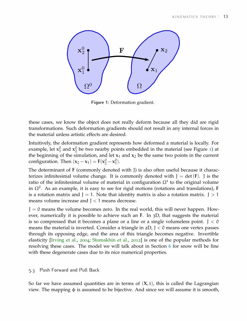
Figure 1: Deformation gradient.
these cases, we know the object does not really deform because all they did are rigidtransformations. Such deformation gradients should not result in any internal forces inthe material unless artistic effects are desired.
Intuitively, the deformation gradient represents how deformed a material is locally. Forexample, let x01 and x02 be two nearby points embedded in the material (see Figure 1) atthe beginning of the simulation, and let x1 and x2 be the same two points in the currentconfiguration. Then (x2 − x1) = F(x
02 − x
01).
The determinant of F (commonly denoted with J) is also often useful because it charac-terizes infinitesimal volume change. It is commonly denoted with J = det (F). J is theratio of the infinitesimal volume of material in configuration Ωt to the original volumein Ω0. As an example, it is easy to see for rigid motions (rotations and translations), Fis a rotation matrix and J = 1. Note that identity matrix is also a rotation matrix. J > 1means volume increase and J < 1 means decrease.
J = 0 means the volume becomes zero. In the real world, this will never happen. How-ever, numerically it is possible to achieve such an F. In 3D, that suggests the materialis so compressed that it becomes a plane or a line or a single volumeless point. J < 0
means the material is inverted. Consider a triangle in 2D, J < 0 means one vertex passesthrough its opposing edge, and the area of this triangle becomes negative. Invertibleelasticity [Irving et al., 2004; Stomakhin et al., 2012] is one of the popular methods forresolving these cases. The model we will talk about in Section 6 for snow will be finewith these degenerate cases due to its nice numerical properties.
5.3 Push Forward and Pull Back
So far we have assumed quantities are in terms of (X, t), this is called the Lagrangianview. The mapping φ is assumed to be bijective. And since we will assume it is smooth,

kinematics theory 14
this means that the sets Ω0 and Ωt are homeomorphic/diffeomorphic under φ. This isassociated with the assumption that no two different particles of material ever occupy thesame space at the same time. This means that ∀x ∈ Ωt, ∃!X ∈ Ω0 such that φ(X, t) = x.In other words, there exist an inverse mapping φ−1(·, t) : Ωt → Ω0. This means thatany function over one set can naturally be thought of as a function over the other setby means of change of variables. We denote this interchange of independent variableas either push forward (taking a function defined over Ω0 and defining a counterpartover Ωt) or vice versa (pull back). For example, given G : Ω0 → R the push forwardg(·, t) : Ωt → R is defined as g(x, t) = G(φ−1(x, t)). Similarly, the pull back of g isG(X) = g(φ(X, t), t) which can be seen to be exactly G(X) by definition of the inversemapping.
The push forward of a function is sometimes referred to as Eulerian (a function of x)and the pull back function is sometimes referred to as Lagrangian (a function of X).As previously defined in Equation 4 and 5, the velocity and acceleration functions areLagrangian. Let’s rewrite them here:
V(X, t) =∂φ
∂t(X, t) (8)
A(X, t) =∂2φ
∂t2(X, t) =
∂V
∂t(X, t). (9)
It is also useful to define Eulerian counterparts. That is, using push forward,
v(x, t) = V(φ−1(x, t), t), (10)
a(x, t) = A(φ−1(x, t), t). (11)
With this, we can also see that the pull back formula are
V(X, t) = v(φ(X, t), t), (12)A(X, t) = a(φ(X, t), t). (13)
With this notion of a and v we can see that (using chain rule)
A(X, t) =∂
∂tV(X, t) =
∂v
∂t(φ(X, t), t) +
∂v
∂x(φ(X, t), t)
∂φ
∂t(X, t). (14)
Using index notation, this can be written as
Ai(X, t) =∂
∂tVi(X, t) =
∂vi∂t
(φ(X, t), t) +∂vi∂xj
(φ(X, t), t)∂φj
∂t(X, t). (15)
where summation is implied on the repeated index j.
Combining Equation 8 and 10, we have
vj(x, t) =∂φj
∂t(φ−1(x, t), t). (16)

kinematics theory 15
Combining Equation 11 and 15, we have
ai(x, t) = Ai(φ−1(x, t), t) =∂vi∂t
(x, t) +∂vi∂xj
(x, t)vj(x, t) (17)
where we used x = φ(φ−1(x, t), t) (by definition).
We thus get a seemingly non-intuitive result:
ai(x, t) 6= ∂vi∂t
(x, t). (18)
5.4 Material Derivative
Although the relationship between the Eulerian a and v is not simply via partial differ-entiation with respect to time, the relationship is a common one and it is often called thematerial derivative. The notation
D
Dtvi(x, t) =
∂vi∂t
(x, t) +∂vi∂xj
(x, t)vj(x, t) (19)
is often introduced so thata =
D
Dtv. (20)
For a general Eulerian function f(·, t) : Ωt → R, we use this same notation to mean
D
Dtf(x, t) =
∂f
∂t(x, t) +
∂f
∂xj(x, t)vj(x, t). (21)
Note that DDtf(x, t) is the push forward of ∂
∂tF where F is a Lagrangian function withF(·, t) : Ω0 → R. F is the pull back of f. This rule of pushing forward ∂
∂tF(X, t) to DDtf(x, t)
is very useful, and should always be kept in mind.
The deformation gradient is usually thought of as Lagrangian. That is, most of the timewhen this comes up in the physics of a material, the Lagrangian view is the dominant one.There is however a useful evolution of the Eulerian (push forward) of F(·, t) : Ω0 → Rd×d.Let f(·, t) : Ωt → Rd×d be the push forward of F, then
D
Dtf =
∂v
∂xf or
D
Dtfij =
∂vi∂xk
fkj (22)
with summation implied on the repeated index k. We can see this because
∂
∂tFij(X, t) =
∂
∂t
∂φi∂Xj
(X, t) =∂Vi∂Xj
(X, t) =∂vi∂xk
(φ(X, t), t)∂φk∂Xj
(X, t), (23)

kinematics theory 16
where the last equality comes from differentiating Equation 12. In some literature (in-cluding [Bonet and Wood, 2008] and [Klar et al., 2016]), Equation 22 is written usingsymbol F instead of f as
F = (∇v)F orDF
Dt= (∇v)F, (24)
while the formula F = ∂∂X
(∂φ∂t
)also appears. When written in such ways, F and f are
undistinguished and F is used for both time derivatives in the two spaces. It is fine to doso as long as F = F(X, t) or F = F(x, t) is clearly specified in the context. Otherwise, weprefer to keep using F to denote the Lagrangian one, and f for the Eulerian one to avoidconfusion.
Equation 23 will play an important role in deriving the discretized F update on eachMPM particle (Section 9.4).
5.5 Volume and Area Change
Assume there is a tiny volume dV at the material space, what is the corresponding valueof dv in the world space? Consider dV being defined over the standard basis vectorse1,e2,e3 with dV = dL1e1 · (dL2e2 × dL3e3), where dLi are tiny numbers, dLi = dLiei.Then we have
dV = dL1dL2dL3. (25)
The corresponding deformed vectors in the world space are
dli = FdLi. (26)
It can be shown that dl1dl2dl3 = JdL1dL2dL3 or dv = JdV where J = det(F).
Given this property, for any function G(X) or g(x, t), it is very common to use the pushforward/pull back when changing variables for integrals defined over subsets of eitherΩ0 or Ωt. That is ∫
Btg(x)dx =
∫B0G(X)J(X, t)dX, (27)
where Bt is an arbitrary subset of Ωt, B0 is the pre-image of Bt under φ(·, t), G is the pullback of g and J(X, t) is the deformation gradient determinant.
Similar analysis can be done for areas. Consider an arbitrary tiny area dS in Ω0, denotethe corresponding area in Ωt with ds. Assuming their normals are N and n respectively,
dS = (dS)N, (28)ds = (ds)n. (29)

hyperelasticity 17
Consider another tiny vector dL (with corresponding deformed version dl) that deter-mines a tiny volume when combined with dS (ds), we have
dV = dS · dL, (30)dv = ds · dl. (31)
Combining this with the previous result dv = JdV , we get
JdS · dL = ds · (FdL), (32)
where we have used dl = FdL. Equation 32 needs to be true for any dL. That results inthe relationship
ds = F−T JdS, (33)
ornds = F−T JNdS. (34)
We can then use this relation ship to write the surface integrals as∫∂Bth(x, t) ·n(x)ds(x) =
∫∂B0H(X) · F−T (X, t)N(X)J(X, t)dS(X) (35)
where H : Ω0 → Rd is the pull back of h : Ωt → Rd, n(x) is the unit outward normal of∂Bt at x and N(X) is the unit outward normal of ∂B0 at X. These relationships are veryuseful when deriving the equations of motion.
6 hyperelasticity
It is more natural to introduce the physical meaning of stress when deriving the gov-erning equations (conservation of momentum) in Section 7. For now we simply in-troduce the fact that stress is related to strain (or deformation gradient in our case)through some “constitutive relationship”. The stress is a field that exists in the wholedomain. There are multiple stress definitions available. For example, the Cauchy stressis σ(·, t) : Ωt → Rd×d. Discretely stress is a small tensor (matrix) at each evaluated point.
A constitutive model relating the state (such as deformation gradient F) to the stress isneeded for governing the material responses under deformations. For perfectly hyper-elastic materials the constitutive relation is defined through the potential energy, whichincreases with non-rigid deformation from the initial state.
In this section we focus on elastic materials as well as an inexact but practically easy-to-use plastic model. The models described below have been successfully used for elasticobjects, sand, snow, lava and many other materials in the MPM publications and movies.

hyperelasticity 18
6.1 First Piola-Kirchoff Stress
For traditional solids, we prefer to express strain stress relationship using deformationgradient and first Piola-Kirchoff stress because they are more naturally expressed in thematerial space. Hyperelastic materials are those elastic solids whose first Piola-Kirchoffstress P can be derived from an strain energy density function Ψ(F) via
P =∂Ψ
∂F. (36)
With index notation, this means
Pij =∂Ψ
∂Fij. (37)
ψ(F) is the elastic energy density function (a scalar function) designed to penalize non-rigid F. P is discretely a small matrix with the same dimensions as F.
Note that it is easy to relate P to the Cauchy stress σ which is sometimes more commonin the engineering literature via
σ =1
JPFT =
1
det(F)∂ψ
∂FFT . (38)
The material behavior is defined via the interaction of φ and the stress σ or P. Forhyperelastic materials, the stress is a function of the change in shape, as expressed viathe deformation gradient. Note that the motion of the material is rigid if
φ(X, t) = R(t)X+ t(t) (39)
where RTR = I, det(R) = 1 and t : [0,∞) → Rd. I.e. R is the rotation and t is thetranslation. Note that in this case, F = R. Hyperelastic materials penalize deformationvia stress that arises from an energy that penalizes deviation of F from orthogonal. Thiscan be written as
P =∂Ψ
∂F, Ψ(F) = Ψ(FTF). (40)
In other words, the energy does not change (and has a minimum) if F is orthogonal.FTF is often denoted with C (right Cauchy-Green tensor). If the material is isotropic(meaning that response to deformation is material direction independent), then we canfurther simplify the energy by writing it as a function of the invariants of C:
Ψ = Ψ(I1, I2, I3) (41)
where Ii are the coefficients of the characteristic polynomial of FTF (often called theisotropic invariants) as
I1 = tr(C), (42)I2 = tr(CC), (43)
I3 = det(C) = J2. (44)

hyperelasticity 19
In graphics, it has been convenient to further write this as
Ψ(F) = Ψ(Σ(F)) (45)
where F = UΣVT is the graphics/mechanics favored “Polar SVD” [Irving et al., 2004;McAdams et al., 2011; Gast et al., 2016] (where both [McAdams et al., 2011] and [Gastet al., 2016] release open source code for rapidly computing it). It is called “Polar SVD”for historical reasons. Mainly, U and V are rotations, and the Polar decomposition F =
RS can be reconstructed via R = UVT and S = VΣVT , where R is the closest rotation toF [Gast et al., 2016] and S is symmetric.
The isotropic invariants can be written in terms of the singular values so this is alwayspossible. This construction of the constitutive response to deformation can be done intu-itively in terms of Σ(F), however it does require differentiating the singular values as afunction of F to get the stress (and stress derivatives) and this requires careful derivation.
6.2 Neo-Hookean
Neo-Hookean is one of the most common nonlinear hyperelastic models for predictinglarge deformations of elastic materials. The energy density function for this model is
Ψ(F) =µ
2
(tr(FTF) − d
)− µ log(J) +
λ
2log2(J), (46)
where d = 2 or 3 denotes the problem dimension, µ and λ are related to Young’s modulusE and Poisson’s ratio ν via
µ =E
2(1+ ν), λ =
Eν
(1+ ν)(1− 2ν). (47)
It is easy to see that when F is a rotation, Ψ(F) = 0. For a non-inverted F (meaningJ > 0), Ψ(F) > 0. The energy density function is adequate to describe a hyperelasticsolid. For force computations, Equation 36 is needed to provide P as a function of F. ForNeo-Hookean, the result is
P = µ(F− F−T ) + λ log(J)F−T . (48)
Note that ∂P∂F is further needed for implicit integration. We provide in Section 6.4 a
practical way to do so.
6.3 Fixed Corotated Constitutive Model
Another simple and widely used model that is defined from the Singular Value Decom-position (SVD) is the so called fixed corotated model. This is called “fixed" because it is a

hyperelasticity 20
small modification to a commonly used model called corotated linear elasticity commonin the computer graphics literature. Assuming the polar SVD F = UΣVT , the energy forfixed corotated model is
Ψ(F) = Ψ(Σ(F)) = µ
d∑i=1
(σi − 1)2 +
λ
2(J− 1)2 (49)
where of course J =∏di=1 σi. Expanding the µ term in the formula we have
µ
d∑i=1
(σi − 1)2 = µ
(d∑i=1
σ2i − 2
d∑i=1
σi + d
). (50)
It can be shown that
∂
∂F
d∑i=1
σ2i = 2F and∂
∂F
d∑i=1
σi = R (51)
where F = RS is the polar decomposition of F (R a rotation matrix and S symmetric).This can of course be defined from the SVD of F as F = UVTVΣVT . I.e. R = UVT andS = VΣVT . Combining all of this, we have
P(F) =∂ψ
∂F(F) = 2µ (F−R) + λ(J− 1)JF−T . (52)
The second derivatives require a bit more care but can be computed relatively easily.
We first do it by computing differentials (which will results in δP). This will be usefulfor a matrix free implementation of the implicit solver.
∂2Ψ
∂F∂F: δF = δ
(∂Ψ
∂F
)(53)
= δ(2µ(F−R) + λ(J− 1)JF−T ) (54)= 2µδF− 2µδR+ λJF−TδJ+ λ(J− 1)δ(JF−T ) (55)= 2µδF− 2µδR+ λJF−T (JF−T : δF) + λ(J− 1)δ(JF−T ) (56)
Since JF−T is a matrix whose entries are polynomials in the entries of F, δ(JF−T ) =∂∂F(JF
−T ) : δF can readily be computed directly. That leaves the task of computing δR.
δF = δRS+RδS (57)RTδF = (RTδR)S+ δS (58)
RTδF− δFTR = (RTδR)S+S(RTδR) (59)
Here we have taken advantage of the symmetry of δS and the skew symmetry of RTδR.There are three independent components of RTδR, which we can solve for directly. Theequation is linear in these components, so RTδR can be computed by solving a 3 × 3system. Finally, δR = R(RTδR).

hyperelasticity 21
6.4 A Practical Differentiation Strategy for Isotropic Elasticity
Here we provide a practical way (originated from [Stomakhin et al., 2012]) to compute Pand ∂P
∂F (either the tensor or the differential δP) for any general isotropic elastic material.This method will utilize a symbolic software package. We will discuss the Mathematicaimplementation. A Maple or any other version is straightforward to produce followingthe same logic. For a more thorough discussion on implementing derivative computa-tions that happen a lot in computer graphics applications, we refer to [Schroeder, 2016].
It is worth noting that this strategy can be used for computing other derivatives in diag-onal space that looks similar to ∂P
∂F . For example in some models, the Kirchoff stress τ(instead of first Piola-Kirchoff stress P) is used:
τ = UτUT , (60)
where τ is a diagonal stress measure with each entry being a function of Σ. To compute∂τ∂F , almost exactly the same method discussed below for computing ∂P
∂F can be used.
6.4.1 Computing P
Let’s start with P. For an isotropic material, stress can be computed as
F = UΣVT , (61)
Ψ(F) = Ψ(Σ), (62)
P = UPVT . (63)
Here, P is diagonal with entries ∂Ψ∂σi
.
Here is the proof for P in diagonal space (Equation 63): First, we want to show P(RF) =
RP(F) for any rotation R. Consider any model (doesn’t even need to be isotropic), rota-tion after deformation shouldn’t change the energy. This means Ψ(F) = Ψ(RF). Take thedifferentials to this equation, we get
δΨ =∂Ψ
∂F(F) : δF =
∂Ψ
∂F(RF) : δ(RF)
(P(F)) : (δF) = (P(RF)) : δ(RF)
(P(F)) : (δF) = (P(RF))ijRikδFkj
(P(F)) : (δF) = (RTP(RF)) : δF
P(F) = RTP(RF)
RP(F) = P(RF)
Similar, if we assume an isotropic material, we can use Ψ(FR) = Ψ(F) to prove P(FR) =P(F)R for any rotation R. Using these two qualities for P, we have
P(F) = P(UΣVT ) = UP(Σ)VT = UPVT . (64)

hyperelasticity 22
6.4.2 Computing ∂P/∂F or δP
The idea is similar to the one for P. Take any two rotations R and Q, use the result for P,we have
P(F) = P(RRTFQQT ) = RP(RTFQ)QT . (65)
Call K = RTFQ, we haveP(F) = RP(K)QT (66)
Now take the differential (and keep in mind that R and Q should be treat as constants):
δP = R
[∂P
∂F(K) : δ(K)
]QT (67)
= R
[∂P
∂F(K) : (RTδFQ)
]QT . (68)
Since R and Q are freely chosen, we choose R = U and Q = V, then K = Σ. The formulathen becomes
δP = U
[∂P
∂F(Σ) : (UTδFV)
]VT . (69)
This gives us δP. For the tensor ∂P/∂F, we adopt the index notation:
(δP)ij = Uik
(∂P
∂F(Σ)
)klmn
UrmδFrsVsnVjl (70)
(δP)ij =
(∂P
∂F(F)
)ijrs
δFrs (71)
These two equations need to hold for any δF, revealing(∂P
∂F(F)
)ijrs
=
(∂P
∂F(Σ)
)klmn
UikUrmVsnVjl (72)
So the remaining problem is computing ∂P∂F (Σ). We show how to do it in 3D.
First, we need to use Rodrigues’ rotation formula. It says any rotation matrix can bewritten in terms of a unit vector k and an rotation angle θ:
R = I+ sin(θ)K+ (1− cos(θ))K2, (73)
where K is the skew-symmetric cross-product matrix of k. This means every rotation ma-trix has only 3 degree of freedoms r1, r2, r3, then k = r
|r|, θ = |r|. So, we can parametrize
rotation matrix U and V with 3 numbers for each.
Now we have the following code for defining F in terms of s1, s2, s3,u1,u2,u3, v1, v2, v3,where U and V are defined by ui and vi with Rodrigues’ rotation formula, si are thesingular values from Σ.

hyperelasticity 23
1 id=I d e n t i t y M a t r i x [ 3 ] ;2 var = s1 , s2 , s3 , u1 , u2 , u3 , v1 , v2 , v3 ;3 Sigma=DiagonalMatrix [ s1 , s2 , s3 ] ;4 cp [ k1_ , k2_ , k3_ ]=0 , −k3 , k2 , k3 ,0 ,−k1 , −k2 , k1 , 0 ;5 vV=v1 , v2 , v3 ;6 vU=u1 , u2 , u3 ;7 nv=Sqrt [ Dot [vV , vV ] ] ;8 nu=Sqrt [ Dot [vU, vU ] ] ;9 UU=cp [ u1 , u2 , u3 ]/nu ;
10 VV=cp [ v1 , v2 , v3 ]/nv ;11 U=id+Sin [ nu ]∗UU+(1−Cos [ nu ] ) ∗UU.UU;12 V=id+Sin [ nv ]∗VV+(1−Cos [ nv ] ) ∗VV.VV;13 F=U. Sigma . Transpose [V ] ;
where cp is a function for generating the cross-product matrix (corresponding to com-puting K in Equation 73).
From now on, we write the 3× 3× 3× 3 tensor ∂P∂F (Σ) and any other such tensors to 9× 9matrices. That means each 3× 3 matrix is now a size-9 vector. It is easy to see the old∂Pij∂Fkl
is now∂P3(i−1)+j∂F3(k−1)+l
. We further call vector S = s1, s2, s3,u1,u2,u3, v1, v2, v3 being theparametrization of F. Then we can apply the chain rule
∂P
∂F(Σ) =
∂P
∂S(Σ)
∂S
∂F(Σ) (74)
Here are the Mathematica code for computing them. Note that we achieve F = Σ bytaking the limit u1,u2,u3, v1, v2, v3 = +ε, which correspond to nearly zero rotations.
1 dFdS=D[ F l a t t e n [ F ] , var ] ;2 dFdS0=dFdS / . u1−>e , u2−>e , u3−>e , v1−>e , v2−>e , v3−>e ;3 dFdS1=Limit [ dFdS0 , e−>0 , Direc t ion −>−1];4 dSdF0=Inverse [ dFdS1 ] ;5 Phat=DiagonalMatrix [ t1 [ s1 , s2 , s3 ] , t 2 [ s1 , s2 , s3 ] , t 3 [ s1 , s2 , s3 ] ] ;6 P=U. Phat . Transpose [V ] ;7 dPdS=D[ F l a t t e n [ P ] , var ] ;8 dPdS0=dPdS / . u1−>e , u2−>e , u3−>e , v1−>e , v2−>e , v3−>e ;9 dPdS1=Limit [ dPdS0 , e−>0 , Direc t ion −>−1];
10 dPdF=Simpl i fy [ dPdS1 . dSdF0 ] ;
Note ’Direction->-1’ in Mathematica means taking the limit from large values to thesmall limit value. The Mathematica computation result will be given in terms of thesingular values and P. One can then take the formula for implementing them in the code.[Stomakhin et al., 2012] gives the result where ∂P/∂F (size 9× 9 matrix) is permuted tobe a block diagonal matrix with diagonal blocks A3×3,B2×212 ,B2×213 ,B2×223 , where
A =
ψ,σ1σ1 ψ,σ1σ2 ψ,σ1σ3ψ,σ2σ1 ψ,σ2σ2 ψ,σ2σ3ψ,σ3σ1 ψ,σ3σ2 ψ,σ3σ3
(75)

hyperelasticity 24
and
Bij =1
σ2i − σ2j
(σiψ,σi − σjψ,σj σjψ,σi − σiψ,σjσjψ,σi − σiψ,σj σiψ,σi − σjψ,σj
). (76)
The division by σ2i − σ2j is problematic when two singular values are nearly equal or
when two singular values nearly sum to zero. The latter is possible with a conventionfor permitting negative singular values (as in invertible elasticity [Irving et al., 2004;Stomakhin et al., 2012]).
Expanding Bij in terms of partial fractions yields the useful decomposition
Bij =1
2
ψ,σi − ψ,σj
σi − σj
(1 1
1 1
)+1
2
ψ,σi + ψ,σj
σi + σj
(1 −1
−1 1
). (77)
Note that if ψ is invariant under permutation of the singular values, then ψ,σi → ψ,σj asσi → σj. Thus, the first term can normally be computed robustly for an isotropic modelif implemented carefully. The other fraction has deeper implications. This term can becomputed robustly if ψ,σi + ψ,σj → 0 as σi + σj → 0. This property is unfavorable, as itmeans the constitutive model will have difficulty recovering from many inverted configu-rations. Since we are usually interested in models with robust behavior under inversion,this term will necessarily be unbounded under some circumstances. We address this byclamping the magnitude of the denominator to not be smaller than 10−6 before divisionto bound the derivatives.
For 2D, a rotation matrix is now simply paremetrized with a single θ where the recon-struction is
R =
(cos θ − sin θsin θ cos θ
).
The 2D version of the whole Mathematica code is
1 id=I d e n t i t y M a t r i x [ 2 ] ;2 var = s1 , s2 , u1 , v1 ;3 S=DiagonalMatrix [ s1 , s2 ] ;4 U= Cos [ u1 ] ,− Sin [ u1 ] , Sin [ u1 ] , Cos [ u1 ] ;5 V= Cos [ v1 ] ,− Sin [ v1 ] , Sin [ v1 ] , Cos [ v1 ] ;6 F=U. S . Transpose [V ] ;7 dFdS=D[ F l a t t e n [ F ] , var ] ;8 dFdS0=dFdS / . u1−>e , v1−>e ;9 dFdS1=Limit [ dFdS0 , e−>0 , Direc t ion −>−1];
10 dSdF0=Inverse [ dFdS1 ] ;11 Phat=DiagonalMatrix [ t1 [ s1 , s2 ] , t 2 [ s1 , s2 ] ] ;12 P=U. Phat . Transpose [V ] ;13 dPdS=D[ F l a t t e n [ P ] , var ] ;14 dPdS0=dPdS / . u1−>e , v1−>e ;15 dPdS1=Limit [ dPdS0 , e−>0 , Direc t ion −>−1];16 dPdF=Simpl i fy [ dPdS1 . dSdF0 ] ;

hyperelasticity 25
original rest shape
new rest shape
current shape
FP
FE
F
Figure 2: Multiplicative decomposition of the deformation gradient.
6.5 Snow Plasticity
Snow constitutive behavior depends on a very wide range of complex factors. There aremany different models used depending on the conditions of interest. Much of the dy-namic behavior can be approximated with a relatively simple elasto-plastic assumption.We will use a simple large-strain plastic flow model combined with a hardening effect.
We represent plasticity by factoring deformation gradient into elastic and plastic parts as
F = FEFP. (78)
The deformation gradient is a measure of how a material has locally rotated and de-formed due to its motion. By factoring the deformation gradient in this way, we dividethis deformation history into two pieces. The plastic part, FP, represents the portion ofthe material’s history that has been forgotten. If a metal rod is bent into a coiled spring,the rod forgets that it used to be straight; the coiled spring behaves as though it was al-ways coiled (see Figure 2). The twisting and bending involved in this operation is storedin FP. If the spring is compressed slightly, the spring will feel strain (deformation). Thisis elastic deformation, which is stored in FE. The spring remembers this deformation. Inresponse, the material exerts stress to try to restore itself to its coiled shape. In this way,we see that only FE should be used to compute stress. The full history of the metal rodconsists of being bent into a spring shape (FP) and then being compressed (FE).
The elastic response is only a function of FE. Intuitively, this states that the deformationin the local transition to FP is permanent. In a sense, Fp comes to represent a new lo-cal rest state of the material. This transition to permanent deformation is typically inresponse to large deformation. A simple example of this would be denting an aluminumcan. Once dented, all elastic response will be to displacement from the dented config-uration. Most models define the decomposition in response to a stress based condition.However, for our case it will be more intuitive to think of the constraint as defined on the

hyperelasticity 26
singular values of F itself. This will give us more visual control over the plasticity effect.Specifically, we will enforce that the singular values σEi of FE are in [1− θc, 1+ θs] forsome small constants θc and θs. This will be done with the following procedure. Given
Fn = FnEFnP , (79)
(where the singular values σnEi of FnE satisfy the constraint of lying in [1− θc, 1+ θs]) anda new Fn+1, we will first assume that all new deformation introduced in the transitionfrom Fn to Fn+1 was elastic. That is we will first assume that given a new Fn+1, it can bedecomposed as
Fn+1 = Fn+1E FnP . (80)
In so doing, this defines Fn+1E as
Fn+1E = Fn+1 (FnP)−1 . (81)
In practice it is often more convenient to store FE and FP instead of storing the full F. Thetentative update of F can then be applied to FE directly to give Fn+1E . The next step is toenforce the constraint that the singular values σn+1Ei of Fn+1E satisfy the constraint of lyingin [1− θc, 1+ θs]. That is, we define
σn+1Ei = clamp(σn+1Ei , 1− θc, 1+ θs), i = 1, . . . ,d (82)
Now, assuming the singular value decomposition of Fn+1E is
Fn+1E = Un+1E ΣEVn+1E
T, (83)
we can define Fn+1E from the clamped singular values Σn+1E as
Fn+1E = Un+1E Σn+1E Vn+1E
T. (84)
Of course with this definition of Fn+1E we still need to maintain the same decompositionof F so we would need to determine a new Fn+1P such that
Fn+1 = Fn+1E Fn+1P . (85)
But of course, given that we know Fn+1 and Fn+1E , the new plastic component of thedeformation gradient is
Fn+1P =(Fn+1E
)−1Fn+1. (86)
Snow will tend to get more rigid under compression. This phenomenon is often calledhardening. We use a simple modification to our constitutive model to add this effect.Specifically, we let the Lame coefficients µ and λ increase under compression and de-crease under extension. The reduction in material strength under extension facilitatesbreak-up and fracture of the snow. This is an important property for a wide range ofvisual phenomena. We quantify this hardening effect as
µ(FP) = µ0eξ(1−JP), λ(FP) = λ0eξ(1−JP) (87)

governing equations 27
where µ0 and λ0 are the Lame parameters as set from the original Young’s modulus andPoisson ratio. ξ is a hardening parameter that we typically use something between 3 and10. Also, JP = det (FP). It is also important to include some safeguards to prevent µ andλ becoming too large. This can be simply done by requiring a numerical clamping boundon ξ(1− JP).
It can also be seen from the derivation that instead of storing Fp, keeping track of Jp isenough as long as we know how to get Fn+1E from the time n quantities. For MPM this isindeed the case.
This hardening model is designed with the intuition that when snow is stretched, itbecomes softer (to allow fracture). When it is compressed, it becomes stiffer like packinga snow ball. The rule in Equation 87 is just an empirical formula. Being creative on therules will help produce more versatile and artistic material behaviors.
A more rigorously derived plasticity model needs to obey the second law of thermody-namics as well as enforcing JP = 1 (plasticity deformation should not change the materialvolume). We refer to the technical document of [Klar et al., 2016] for a more thoroughdiscussion on this matter.
7 governing equations
The governing equations of interest are conservation of mass and conservation of mo-mentum. We’ll list the result below and provide their derivations in Section 7.1 and 7.2.We further derive the weak form of the force balance in Section 7.3. The weak form isessential for deriving the final temporal and spatial discretization of the equations inSection 9. It is recommended to review Section 5 before looking into the derivations.
Letting V(X, t) = ∂Φ(X,t)∂t =
∂x(X,t)∂t be the velocity defined over X, the Lagrangian view of
the equations are [Gonzalez and Stuart, 2008]
R(X, t)J(X, t) = R(X, 0) Conservation of mass, (88)
R(X, 0)∂V
∂t= ∇X ·P+ R(X, 0)g Conservation of momentum, (89)
where X ∈ Ω0,t > 0. Here R is the Lagrangian mass density which is related to the morecommonly used Eulerian mass density ρ as R(X, t) = ρ(Φ(X, t), t). Note that the massconservation can also be written as ∂
∂t (R(X, t)J(X, t)) = 0.
In Eulerian view, the governing equations are
D
Dtρ(x, t) + ρ(x, t)∇x · v(x, t) = 0 Conservation of mass, (90)
ρ(x, t)Dv
Dt= ∇x ·σ+ ρ(x, t)g Conservation of momentum, (91)

governing equations 28
where v = v(x, t) is the Eulerian velocity, DDt =
∂∂t + v · ∇
x is the material derivative.
As shown in the conservation of momentum, it is more convenient to use the first Piola-Kirchoff stress P in the Lagrangian view, and the Cauchy stress σ in the Eulerian view.
7.1 Conservation of Mass
Let ρ(x, t) be the Eulerian mass density and let R(X, t) be the Lagrangian counterpart(pull back), we have the relationship
R(X, t) = ρ(φ(X, t), t) (92)
ρ(x, t) = R(φ−1(x, t), t). (93)
We can think of ρ to be naturally defined over Ωt as
ρ(x, t) = limε→+0
mass(Btε)∫Btεdx
(94)
where Btε is the ball of radius ε surrounding an arbitrary x ∈ Ωt. This is arguablya natural definition since mass(Btε) should be a measurable quantity. Conservation ofmass can be expressed as
mass(Btε) =∫Btε
ρ(x, t)dx =∫B0ε
R(X, t)JdX =
∫B0ε
R(X, 0)dX = mass(B0ε) (95)
for all Btε ⊂ Ωt (as before, B0ε is the pre-image of Btε under φ(·, t)). The second equalitycomes from using the change of variable result from Section 5.5.
This just says that the mass in Btε (as expressed via an integral of the mass density) shouldnot change with time. This set is associated with a subset of the material at time t and asit evolves in the flow, the material will take up more or less space, but there will neverbe more or less material in the set. Since Btε is arbitrary, it must be true that
R(X, t)J(X, t) = R(X, 0), ∀X ∈ Ω0, t > 0. (96)
Note that J(X, 0) = 1. Alternatively, mass conservation can be written as
∂
∂t(R(X, t)J(X, t)) = 0. (97)
To switch to the Eulerian view, we first notice that
∂
∂t(RJ) =
∂R
∂tJ+ R
∂J
∂t. (98)
Also,∂J
∂t=∂J
∂Fij
∂Fij
∂t= JF−1ji
∂Vi∂Xj
= JF−1ji∂vi∂xk
Fkj = Jδik∂vi∂xk
= J∂vi∂xi
, (99)

governing equations 29
where we have used the determinant differentiation rule
∂J
∂F= JF−T . (100)
Combining Equation 97, 98 and 99, we get
∂R
∂tJ+ RJ
∂vi∂xi
= 0. (101)
Pushing forward on both sides result in the Eulerian view of conservation of mass:
D
Dtρ(x, t) + ρ(x, t)∇ · v(x, t) = 0, ∀x ∈ Ωt, t > 0. (102)
7.2 Conservation of Momentum
Continuum forces are classified as either body forces (e.g. gravity) or surface forces(stress-based). Stress-based forces are first defined via a traction field whose existencewe will assume. The force per area (or traction) field t(·,n, t) : Ωt → Rd is defined viathe relation
forceS(Btε) =∫∂Btε
t(x,n(x))ds(x) (103)
where forceS(Btε) is the net force on an arbitrary Btε exerted from material on the otherside of ∂Btε on material inside Btε. That is, t(x,n, t) is the force per unit area(d =
3)/length(d = 2) that material in the n+ side of the material at the point x exerts onmaterial on the n− side. It can be shown that this implies the existence of a stress field(Cauchy stress) σ(·, t) : Ωt → Rd×d with
t(x,n, t) = σ(x, t)n. (104)
Let v be the Eulerian velocity (with Lagrangian counterpart V). Then conservation ofmomentum is expressed as
d
dt
∫Btε
ρ(x, t)v(x, t)dx =d
dt
∫B0ε
R(X, t)V(X, t)JdX =
∫B0ε
R(X, 0)A(X, t)dX
=
∫∂Btε
σnds(x) +
∫Btε
fextdx (105)
for all Btε ⊂ Ωt in the time t configuration of the material. Here we have added thecontribution of external body force (such as gravity) fext to the change of momentum.fext represents the external body force per unit volume. Therefore the rate of change ofthe momentum in Btε is equal to the net force on Btε as expressed via the Cauchy stressfield plus the external force. It can also be shown that σ(x, t) must be symmetric forconservation of angular momentum [Bonet and Wood, 2008].

governing equations 30
The last equality of Equation 105 can also be written as∫B0ε
R(X, t)J(x, t)A(X, t)dX =
∫∂Btε
σnds(x) +
∫Btε
fext(x, t)dx. (106)
Pushing forward the volume integral on the left side of Equation 106 results in both sidesover Btε:∫
Btε
ρ(x, t)a(x, t)dx =∫∂Btε
σnds(x) +
∫Btε
fextdx =
∫Btε
∇x · σdx+∫Btε
fextdx, (107)
or
ρa = ∇x · σ+ fext, ∀x ∈ Ωt, t > 0. (108)
Alternatively, we can also choose to pull back the right side of Equation 106 using∫∂Btε
σ(x, t)nds(x) =∫∂B0ε
J(X, t)σ(φ(X, t), t)F−T (X, t)Nds(X). (109)
Recall the first Piola Kirchoff stress is related to the Cauchy stress as P = JσF−T , we get∫∂Btε
σ(x, t)nds(x) =∫∂B0ε
P(X, t)Nds(X) =∫B0ε
∇x ·P(X, t)dX. (110)
Compare this with Equation 106 we get the Lagrangian form of conservation of momen-tum: ∫
B0ε
R(X, 0)A(X, t)dX =
∫B0ε
∇x ·P(X, t)dX+
∫B0ε
FextJ(X, t)dX (111)
orR(X, 0)A(X, t) = ∇x ·P(X, t) + Fext(X, t)J(X, t), ∀X ∈ Ω0, t > 0 (112)
where Fext is the pull back of the Eulerian body force per unit volume fext.
7.3 Weak Form
MPM is like the FEM discretization of the stress based forces over the Eulerian grid. Ittherefore uses the weak form of force balance. We can think of it as Lagrangian. Let’signore the external force for simplicity. We can start with the conservation of momentum
R(X, 0)A(X, t) = ∇x ·P(X, t),∀X, t, (113)
orR0Ai = Pij,j, ∀X, t, (114)

material particles 31
where R0 = R(X, 0). So for an arbitrary function Q(·, t) : Ω0 → Rd, let’s compute the dotproduct to Equation 113 and integrate over Ω0 to generate the weak form:∫
Ω0Qi(X, t)R(X, 0)Ai(X, t)dX =
∫Ω0Qi(X, t)Pij,j(X, t)dX (115)
=
∫Ω0
((Qi(X, t)Pij(X, t)
),j −Qi,j(X, t)Pij(X, t)
)dX (116)
=
∫∂Ω0
Qi(X, t)Pij(X, t)Nj(X, t)ds(X)
−
∫Ω0Qi,j(X, t)Pij(X, t)dX. (117)
The quantity PijNj would be specified as a boundary condition. If we let T (X, t) be theboundary force per unit reference area with Ti = PijNj, then we can say that force balanceimplies that ∀Q(·, t) : Ω0 → Rd∫
Ω0Qi(X, t)R(X, 0)Ai(X, t)dX =
∫∂Ω0
QiTids(X) −
∫Ω0Qi,jPijdX . (118)
For MPM, the stress derivatives will be discretized in the current configuration, so wecan push the stress involving integrals to the Eulerian view. Let q be the push forwardof Q with Q(X, t) = q(φ(X, t), t) and q(x, t) = Q(φ−1(x, t), t), we have
Qi,j =∂Qi∂Xj
=∂qi∂xk
∂xk∂Xj
= qi,kFkj. (119)
Further more, recall that
σik =1
JPijFkj,
and define t to be the external force per unit area in the Eulerian configuration (t is thepush forward of T ), Equation 118 becomes∫
Ωtqi(x, t)ρ(x, t)ai(x, t)dx =
∫∂Ωt
qitids(x) −
∫Ωtqi,kσikdx , (120)
where we have pushed forward the volume and surface integrals using the rules de-scribed in Section 5.5. Force balance implies the above holds for an arbitrary q(·, t) :
Ωt → Rd. We call Equation 120 the weak form of force balance in the Eulerian view. TheMPM discretization on the grid will be based on this equation.
8 material particles
Before discretizing the weak form of the force balance (Equation 120), let’s first introducethe material particles (or material points, Lagrangian particles, etc. ) that represents thematerial simulated with MPM.

material particles 32
Recall that the material point method is Lagrangian in the sense that we track actualparticles of material. That is we keep track of mass (mp), velocity (vp) and position (xp)for a collection of material particles p. However, all stress based forces are computed onthe Eulerian grid, so we have to transfer the material state to the Eulerian configurationto incorporate the effects of material forces. Then, we transfer these effects back to thematerial particles and move them in the normal Lagrangian way. The Lagrangian naturemakes advection very trivial compared to pure Eulerian methods (such as grid-basedfluid simulation).
Just like any other PIC/FLIP solvers, MPM solves the governing equation on a back-ground Eulerian grid. The grid acts as a scratch pad. It can be destroyed after each solveand reinitialized in the beginning of the next time step. In practice, it is easy to just usea fixed Cartesian grid.
8.1 Eulerian Interpolating Functions
In each time step of MPM, particles transfer their mass and momentum to the grid nodes.After the grid solve, velocities are transferred back to particles for them to perform the ad-vection step. Both transfers require interpolation functions. Taking a Finite Element view,the Eulerian grid is the essential computational mesh while particles act as quadraturepoints. Therefore, instead of thinking of the interpolation function as a particle ‘kernel’as in SPH, it is more natural (but not necessarily) to let the interpolation functions bedefined over grid nodes.
We can denote the interpolation function at grid node i with Ni(x). Note that i is boldhere because it is usually a multi-index for grid nodes. Specifically, i = (i, j) in 2D,i = (i, j,k) in 3D. When Ni(x) is evaluated at a particle location xp, a shorter notationNi(xp) = wip is often used instead. Intuitively, we are associating with each particlep and grid node i a weight wip which determines how strongly the particle and nodeinteract. If the particle and grid node are close together, the weight should be large. Ifthe particle and node are farther apart, the weight should be small.
We use dyadic products of one-dimensional interpolation functions as our grid basisfunctions as in [Steffen et al., 2008]
Ni(xp) = N(1
h(xp − xi))N(
1
h(yp − yi))N(
1
h(zp − zi)), (121)
where i = (i, j,k) is the grid index, xp = (xp,yp, zp) is the evaluation position, h is thegrid spacing, xi = (xi,yi, zi) is the grid node position. For more compact notation, wewill use wip = Ni(xp) and ∇wip = ∇Ni(xp). While writing them like these, one shouldkeep in mind both Ni and ∇Ni are still functions of arbitrary x. When writing with w, itmeans these functions are evaluated at x = xp.
Choosing a kernel N leads to trade offs with respect to smoothness, computational effi-ciency, and the width of the stencil. We prefer tensor product splines for their compu-

material particles 33
tational efficiency, as they are relatively inexpensive to compute, differentiate, and store.The multi-linear kernel typically employed for FLIP fluid solvers is the simplest of theseoptions, but it is not suitable here. There are two reasons for this (see [Steffen et al.,2008]). The first is that ∇wip would be discontinuous and produce discontinuous forces.The second is that∇wip may be far from zero when wip ≈ 0, leading to large forces beingapplied to grid nodes with tiny weights. MPM typically requires C1 continuity of theinterpolation function to prevent the so called cell-crossing instability. In practice, eitherquadratic B splines or cubic B splines may be used. Quadratic B splines is more compu-tational efficient and memory saving due to a smaller transfer stencil. Cubic B splines onthe other hand, is more expensive but provides wider coverage, therefore less sensitiveto numerical errors such as numerical fracture when they are not desired artistic effects.The cubic kernel is defined with
N(x) =
12 |x|
3 − |x|2 + 23 0 6 |x| < 1
16(2− |x|)3 1 6 |x| < 2
0 2 6 |x|
(122)
where h is the grid spacing. The quadratic kernel is also useful:
N(x) =
34 − |x|2 0 6 |x| < 1
2
12
(32 − |x|
)2 12 6 |x| < 3
2
0 32 6 |x|
(123)
The quadratic and cubic kernels are shown in Figure 3. Though theoretically unstable,linear interpolation functions may still work for certain applications in practice. It is
N(x) =
1− |x| 0 6 |x| < 1
0 1 6 |x|(124)
Computing the gradient is done similarly by differentiating the one dimensional func-tions:
∇Ni(xp) =
1hN′( 1h(xp − xi))N( 1h(yp − yi))N( 1h(zp − zi))
N( 1h(xp − xi))1hN′( 1h(yp − yi))N( 1h(zp − zi))
N( 1h(xp − xi))N( 1h(yp − yi))1hN′( 1h(zp − zi))
where N ′(x) is the derivative of N(x).
8.2 Eulerian/Lagrangian Mass
When representing our material as a finite collection of points, we can assign each pointa subset (B0∆x,p ⊂ Ω0) of the total material. In this way, we can define the mass of thatparticle to be
mnp =
∫Btn∆x,p
ρ(x, tn)dx. (125)

material particles 34
N(x)
Figure 3: Cubic (blue) and quadratic (red) splines used for computing interpolation weights.
With this convention, we can define the following conservative process for transferringmass and momentum (and then velocity) to the nodes of the Eulerian grid. Define
mi =∑p
mpNi(xp) (126)
as the mass of Eulerian grid node i. With this convention, we have∑i
mi =∑i
∑p
mpNi(xp) =∑p
mp
∑i
Ni(xp) =∑p
mp (127)
by the partition of unity assumption on the Ni.
8.3 Eulerian/Lagrangian Momentum
Similarly, we can transfer particle momentum mpvp as (note that we will eventually usea different transfer called APIC described in Section 10.1)
(mv)i =∑p
mpvpNi(xp) (128)
and we can show that ∑i
(mv)i =∑p
mpvp (129)
by the same partition of unity logic. The Eulerian velocity vi is defined as
vi =(mv)imi
. (130)
Note that in this case, the repeated index does not imply summation.

discretization 35
8.4 Eulerian to Lagrangian Transfer
The transfer from Eulerian variables to Lagrangian variables is similar. However, wenever need to transfer mass from the grid to the particles since Lagrangian particle massnever changes. Velocity is simply interpolated as
vp =∑i
viNi(xp). (131)
It is easily verified that this conserves momentum as∑p
mpvp =∑p
mp
∑i
viNi(xp) =∑i
vi∑p
mpNi(xp) =∑i
mivi. (132)
9 discretization
9.1 Discrete Time
We will start by assuming we are at time tn. Recall that the weak forms of the forcebalance equation (Equation 118 and 120) imply∫
Ω0QiR0AidX =
∫∂Ωt
nqitids(x) −
∫Ωtnqi,kσikdx (133)
for all q(x, tn) (or Q(X, tn)). We start by replacing the Lagrangian acceleration Ai(X, tn)with 1
∆t
(Vn+1i − Vni
). We can then push the left hand side forward from Ω0 to Ωt
nto
obtain1
∆t
∫Ωtnqi(x, tn)ρ(x, tn)
(vn+1i (x) − vni (x)
)dx
=
∫∂Ωt
nqi(x, tn)ti(x, tn)ds(x) −
∫Ωtnqi,k(x, tn)σik(x, tn)dx. (134)
Note that with this notation vn : Ωtn → Rd, vn+1 : Ωt
n → Rd (both of them are definedfor x ∈ Ωtn). Therefore vn+1i (x) = Vi(φ
−1(x, tn), tn+1) and vni (x) = Vi(φ−1(x, tn), tn).
We should keep in mind that all the i and k subscripts in Equation 134 are componentindex for dimensions. I.e., i = 1, 2, 3 for 3D and i = 1, 2 for 2D. When we are goingdiscrete in space, we probably want to use indices like i, j,k to denote a grid node. Toavoid confusion, from now on, we can require Greek letters like α,β,γ to denote thecomponent index. This results in rewriting Equation 134 as
1
∆t
∫Ωtnqα(x, tn)ρ(x, tn)
(vn+1α (x) − vnα(x)
)dx
=
∫∂Ωt
nqα(x, tn)tα(x, tn)ds(x) −
∫Ωtnqα,β(x, tn)σαβ(x, tn)dx, (135)

discretization 36
where α,β = 1, 2, ..,d and d is the problem dimension (2 or 3). Now qiα means the αcomponent of the vector quantity q that is stored at node i. Also, qα(x, t) means the αcomponent of the field q(x, t).
9.2 Discrete Space
We can do an FEM style discretization of the spatial terms by replacing qα, vnα and vn+1α
with grid based interpolants as
qα(x, tn) =∑i
qiα(tn)Ni(x), (136)
vnα(x) =∑j
vnjαNj(x), (137)
vn+1α (x) =∑j
vn+1jα Nj(x) (138)
orqnα = qniαNi, v
nα = vnjαNj, v
n+1α = vn+1jα Nj (139)
for short where summation is implied on the repeated index. Force balance (Equation135) can then be viewed as
1
∆t
∫ΩtnqniαNi(x)ρ(x, tn)vn+1jα Nj(x)dx−
1
∆t
∫ΩtnqniαNi(x)ρ(x, tn)vnjαNj(x)dx
=
∫∂Ωt
nqniαNi(x)tα(x, tn)ds(x) −
∫ΩtnqniαNi,β(x)σαβ(x, tn)dx. (140)
for all qiα. This can also be expressed as
qniαδαβmnij
∆tvn+1jβ − qniαδαβ
mnij
∆tvnjβ
=
∫∂Ωt
nqniαNitαds(x) −
∫ΩtnqniαNi,βσαβdx. (141)
where
mnij =
∫ΩtnNi(x)ρ(x, tn)Nj(x)dx (142)
defines the mass matrix. We can pull it back to the material space to get
mnij =
∫Ω0Ni(x(X))R(X, 0)Nj(x(X))dX ≈
∑p
mpNi(xp)Nj(xp). (143)
It is symmetric positive semi-definite because it can be written as BBT (mij =∑p BipBjp)
where Bip =√mpNip so that zTMz > 0 for any z. In practice we can not use this

discretization 37
mass matrix because it may be singular. We’ll see below a “mass lumping” strategy toapproximate the mass matrix with a diagonal and positive definite matrix while keepingconsistent with the particle-grid transfers.
Equation 141 must be true for all choices of qniα. So if we choose them to be
qniα =
1, α = α and i = i0, otherwise
then ∑j
mij
∆t
(vn+1jα − vnjα
)=
∫∂Ωt
nNitαds(x) −
∫ΩtnNi,βσαβdx. (144)
This can be seen as a discrete force balance equation for the i, α degree of freedom onthe grid. We will next show that it can be used as an explicit update rule for the Eulerianmomentum and that the right hand side can be thought of as the αth component of theforce on the ith Eulerian grid node.
As we just mentioned, it is often convenient (though less accurate) to use a mass lumpingsimplification. It is done by replacing the rows in mij with the corresponding row sum,thus making it a diagonal matrix. The row sums (let’s call it mi for row i) are
mi =∑j
∫ΩtnNi(x)ρ(x, tn)Nj(x)dx =
∫ΩtnNi(x)ρ(x, tn)
∑j
Nj(x)dx
=
∫ΩtnNi(x)ρ(x, tn)(x)dx. (145)
We can also use the following approximation (similarly to what we did in Equation 143)∫ΩtnNi(x)ρ(x, tn)dx =
∫Ω0Ni(x(X))R(X, 0)dX ≈
∑p
Ni(xp)mp (146)
since mp ≈ V0pR(Xp, 0). In other words mi can naturally be approximated as mi.
Rewriting mivni as the momentum (mv)ni , we can summarize the discretization as((mv)n+1iα − (mv)niα
)∆t
=
∫∂Ωt
nNi(x)tα(x, tn)ds(x) −
∫ΩtnNi,β(x)σαβ(x, tn)dx . (147)
In other words, since the left hand side is the change in momentum, the right hand sideis approximately the force. Here we have assumed that we have an estimate of the stressσnp ≈ σ(xnp , tn) at each Lagrangian particle xnp , thus∫
ΩtnNi,β(x)σαβ(x, tn)dx ≈
∑p
σpnαβNi,β(x
np)V
np (148)
where Vnp is the volume of Btn
∆x,p, or the volume particle p occupies at time tn.

discretization 38
9.3 Estimating the Volume
We can estimate Vnp with two ways. First, recall that
mp ≈ R(Xp, 0)V0p ≈ ρ(xnp , tn)Vnp . (149)
We can then approximate ρ(xnp , tn) from mni as
ρni =mni
∆xd, (150)
ρ(xnp , tn) ≈∑i
ρni Ni(xnp). (151)
Therefore
Vnp ≈mp∑
imni∆xdNi(xnp)
=mp∆x
d∑im
ni Ni(x
np)
. (152)
Another approach is given as follows. If we have an approximation of the deformationat each Lagrangian particle: Fnp ≈ F(Xp, tn) (which we will usually need for an elasticmaterial), then you can approximate Vnp using Jnp = det(Fnp). Specifically, if we assumewe know the initial volume V0p =
∫B0∆x,p
dx, then
Vnp ≈ V0pJnp . (153)
If we use the formula for the first Piola Kirchoff stress σ = 1JPF
T then we can furtherrewrite Equation 147 and 148 in terms of P instead of σ:∑
p
σpnαβNi,β(x
np)V
np =∑p
1
JnpPnpαγF
npβγ
Ni,β(xnp)V
0pJnp =∑p
PnpαγFnpβγ
Ni,β(xnp)V
0p. (154)
This is the formula that will be more useful in practice because most of our constitutivemodels are expressed in terms of P. Now,(
(mv)n+1iα − (mv)niα
)∆t
=
∫∂Ωt
nNi(x)tα(x, tn)ds(x) −
∑p
PnpαγFnpβγ
Ni,β(xnp)V
0p . (155)
We will next discuss how to approximate the deformation gradient (Fnp) at each La-grangian point (xnp).
9.4 Deformation Gradient Evolution
In order to continue the discussion of time stepping schemes, we need to consider theconstitutive model. So far, the results hold independent of the type of material. We

discretization 39
will generally consider models where the stress depends primarily on the change ofshape in the material as expressed via the deformation gradient (this includes all modelsdiscussed in Section 6). Next, we will discuss how this can be computed in the MPMcontext. The deformation gradient is more difficult to compute for Eulerian methods (orLagrangian methods where there is no mesh, e.g. particle methods). However, we canuse the equation (recall the result from Section 5.4)
∂
∂tF(X, t) =
∂v
∂x(φ(X, t), t)F(X, t) (156)
to update (or evolve) a deformation gradient on each material particle by discretizing ∂v∂x
over the Eulerian grid.
Now let’s reformulate a similar rule discretely. We assume we have the velocity (de-fined over Ωt
n) at time tn+1 as a a function of x only. Specifically, we consider the
function vn+1 : Ωtn → Rd defined as vn+1(x) = V(φ−1(x, tn), tn+1) and also of course
vn+1(φ(X, tn)) = V(X, tn+1). (We have used the same definition in Section 9.1.) With thiswe have
∂
∂tF(X, tn+1) =
∂V
∂X(X, tn+1) =
∂vn+1
∂x(φ(X, tn))F(X, tn). (157)
This is useful because if we further use the approximation
∂
∂tF(Xp, tn+1) ≈
Fn+1p − Fnp∆t
(158)
then
Fn+1p = Fnp +∆t∂vn+1
∂x(xnp)F
np =
(I+∆t
∂vn+1
∂x(xnp)
)Fnp (159)
and of course if we use the grid based interpolation formula for vn+1, i.e.,
vn+1(x) =∑i
vn+1i Ni(x), (160)
∂vn+1
∂x(x) =
∑i
vn+1i
(∂Ni∂x
(x)
)T, (161)
then we have
Fn+1p =
(I+∆t
∑i
vn+1i
(∂Ni∂x
(xnp)
)T)Fnp (162)
as the update rule for Fn+1p given the vn+1i and Fnp .
9.5 Forces as Energy Gradient
The elastic response can be shown to arise from an elastic potential energy. This is truefor both the continuous and discrete cases. For the discrete case, consider xi defined to

discretization 40
be the nodes of the Eulerian grid when xi = xi. In other words, consider temporarilythat we have allowed the nodes of the Eulerian grid to move with a variable defined asxi denoting the imaginary moved node position. We can then temporarily think of thesexi as new Lagrangian degrees of freedom. It is like saying that we switched from havingthe Xp as our Lagrangian particles and switched over to Xi = φ−1(xi, tn) as our newLagrangian particles and with this we say that xn+1i = φ(Xi, tn+1) = xi defines the newconfiguration of our material. If we keep this idea in mind, we can show that the forcesderived in Section 9.2 are related to a discrete potential energy in the case of a certainclass of elastic materials. For hyperelastic materials where the first Piola Kirchoff stressis related to an elastic potential energy density ψ via
P(F) =∂ψ
∂F(F) (163)
as we saw in Section 6, we can define the total potential energy (as a function of themoved node positions x as
e(x) =∑p
ψ(Fp(x))V0p (164)
where x is the full (assembled) vector of all Eulerian xi. Here we think of the deformationgradient as a function of x. This is because we are temporarily thinking of the motionof the material as defined in terms of the Xi = φ−1(xi, tn) and xi. Really, this is anequivalent notion to letting motion be defined via the vn+1i . Specifically we can think ofthem defined as
vn+1i =xi − xi∆t
or xi = xi +∆tvn+1i . (165)
This leads to the particle wise deformation gradient formula of
Fpβγ(x) = Fnpβγ
+∆t∑j
(xjβ − xjβ∆t
)∑τ
Nj,τ(xnp)F
npτγ
. (166)
If we differentiate the energy with respect to xiα (the αth component of xi) we get
∂e
∂xiα(x) =
∑p
∑β,γ
Pβγ(Fp(x))∂Fpβγ
∂xiα(x)V0p. (167)
From the formula for the deformation gradient above, we can see that
∂Fpβγ
∂xiα(x) = δαβ
∑τ
Ni,τ(xnp)F
npτγ
(168)
and if we plug this into Equation 167 we get
∂e
∂xiα(x) =
∑p
Pαγ(Fp(x))FnpτγNi,τ(x
np)V
0p. (169)

explicit time integration 41
Therefore, comparing with the result in Section 9.3, we can see that the force on theEulerian grid node i is
−∂e
∂xiα
x = x0x1...
. (170)
In other words, we can write the momentum update as
(mv)n+1iα = (mv)niα −∆t∂e
∂xiα
x = x0x1...
+∆t
∫∂Ωt
nNi(x)tα(x, tn)ds(x) . (171)
10 explicit time integration
In this section we describe the easiest implementation of MPM with Symplectic Eulertime integration. Most of the formulas in this section are derived in previous sessions.They are restated here to provide a more concise and practitioner friendly reference forimplementing MPM. We first discuss some separate modules and then state the full MPMalgorithm.
10.1 APIC Transfers
The Affine Particle-In-Cell (APIC) method [Jiang et al., 2015] is recommended for particle-grid transfers due to its nice numerical properties. We ignore the time superscripts herefor notation simplicity.
The transfer from particles to grid is
mi =∑p
wipmp, (172)
mivi =∑p
wipmp(vp +Bp(Dp)−1(xi − xp)), (173)
where Bp is a matrix quantity stored at each particle (just like mass, position and velocity),Dp is given by
Dp =∑i
wip(xi − xp)(xi − xp)T (174)

explicit time integration 42
and is derived by preserving affine motion during the transfers. The correspondingtransfer from the grid back to particles is
vp =∑i
wipvi, (175)
Bp =∑i
wipvi(xi − xp)T . (176)
Conveniently, Dp takes on a surprisingly simple form in the case of the quadratic (Dp =14∆x
2I) and cubic (Dp = 13∆x
2I) interpolation stencils commonly used for MPM. Notethat for these interpolating stencils, multiplying by (Dp)
−1 amounts to a constant scalingfactor.
If (though not recommended) linear spline is used for the interpolation function, to pre-vent singular Dp, an alternative formulation of APIC particle to grid is given as
mi =∑p
wipmp, (177)
mivi =∑p
wipmp(vp + Cp(xi − xp)), (178)
and the grid to particle transfer is
vp =∑i
wipvi, (179)
Cp =∑i
vi
(∂Ni∂x
(xp)
)T. (180)
Note that in this case, Cp is just the Eulerian velocity gradient evaluated at xp, which wehave already computed for evolving Fp.
10.2 Deformation Gradient Update
In the beginning of each time step, the grid node locations are always on a undeformedregular grid. Let’s call them xni . The sup-script n is not necessary if we use the samegrid all the time but we’ll keep it here for notation convention. The deformation gradientof each particle can be updated following the motion of the grid. If we assume a gridvelocity field vn+1i , it can be shown that the update rule for F is
Fn+1p =
(I+∆t
∑i
vn+1i (∇wnip)T
)Fnp . (181)

explicit time integration 43
10.3 State Update
Symplectic Euler time integration on the grid implies
xn+1i = xni +∆tvn+1i , (182)
vn+1i = vni +∆tfi(xni )/mi. (183)
One way of thinking about the grid motion is
x = x(v), (184)
i.e. the grid node positions are simply a function of grid node velocities via Equation 182.Therefore
fni = fi(xni ) = fi(x(0)), (185)
i.e., the explicit force is simply the force assuming zero grid motion. Using Equation 182,we can rewrite Equation 181 as
Fp(x) =
(I+∑i
(xi − xni )(∇w
nip)
T
)Fnp , (186)
so that Fp is a function of grid node locations x.
10.4 Forces
MPM Forces are defined on grid nodes. As we’ve seen earlier, for hyperelastic solids, theforce can be derived either from the weak form of momentum equation or as the gradientof total potential energy. The later is simpler and often used as long as there is a welldefined potential energy. Here we focus on hyperelastic solids.
As mentioned before, we assume a deformation gradient based hyperelastic energy den-sity. The total elastic potential energy is then
e =∑p
V0pΨp(Fp), (187)
where V0p is the material space volume of particle p.
Nodal elastic force is the negative gradient of the total potential energy evaluated atnodal positions. Using Equation 186, the MPM spatial discretization of the stress-basedforces is given as
fi(x) = −∂e
∂xi(x) = −
∑p
V0p
(∂Ψp
∂F(Fp(x))
)(Fnp)
T∇wnip. (188)

explicit time integration 44
This is the force acting on grid node i resulting from elastic stresses of its nearby particles.In the case of Symplectic Euler, the force is easily written as
fni = fi(xni ) = −
∑p
V0p
(∂Ψp
∂F(Fnp)
)(Fnp)
T∇wnip, (189)
which fully depends on the existing particle/grid weights and particle attributes. Al-ternatively if we don’t have the energy density, the force can also be written using theCauchy stress,
fni = fi(xni ) = −
∑p
Vnpσnp∇wnip, (190)
this comes from the weak form.
10.5 MPM Scheme: Full Algorithm
Here we outline the full update scheme for Symplectic Euler MPM. The particles areassumed to have already been initialized (i.e. each particle has a mass mp, volumeV0p, initial position xp, initial velocity vp, affine matrix Bp and their material-relatedparameters (such as µ and λ in the case of Neo-Hookean).
1. Particle to grid transfer (P2G). Using the APIC formula from Section 10.1, the firststep is to transfer particle quantities to the grid. In particular, this step computesgrid mass and momentum.
2. Compute grid velocities. vi =mivimi
. For nodes with mass equals to 0, mi and viare manually reset to 0. One would traditionally think this requires a floating pointthreshold when implementing this step. However in practice directly comparingagainst 0.0f will not produce any unstable behavior or overflow. This is becauseeven though you may get large forces on small mass nodes, the effect is scaledby the weight again when transferrring back to particles. In fact, hard coding athreshold will cause various problems such as drifting of total momentum.
3. Identify grid degree of freedoms. This step is important for implementation effi-ciency. We label the grid nodes with nonzero masses to be the actually degree offreedoms. All other nodes will remain static and are not considered being part ofthe solver unknowns.
4. Compute explicit grid forces fni using Equation 189.
5. Grid velocity update using Equation 183. This step should take the boundaryconditions or collision objects into account. In the case of explicit integration, eachnodal velocity can be independently set to the desired value due to Dirichlet bound-ary conditions or rigid object collisions. See Section 12.1 for more details on how todeal with collision objects.
implicit time integration 45
6. Update particle deformation gradient using Equation 181. Note that we neveractually moved the grid or computed any new grid x. The motion is imaginary andonly velocities are explicitly stored.
7. Grid to particle transfer (G2P). This step computes new particle velocities vn+1p
and affine matrices Bn+1p with the scheme given in Section 10.1.
8. Particle advection. Finally particles are advected with their new velocities: xn+1p =
xnp +∆tvn+1p . Note that this is only true when APIC is used. In a FLIP or FLIP-PIC-
blending transfer scheme, xn+1p =∑i xn+1i wip should be used instead (note that
these two formulas are equivalent in the PIC or APIC case).
11 implicit time integration
For implicit time integration, the main difference from explicit is the grid velocity updatestep in the MPM algorithm.
11.1 Force Derivative
Recall that the total elastic potential energy can be expressed in terms of the energydensity Ψ as ∫
Ω0Ψ(F(X))dX, (191)
where Ω0 is the undeformed configuration of the material. The MPM spatial discretiza-tion of the stress-based forces is equivalent to differentiation of a discrete approximationof this energy with respect to the Eulerian grid node material positions. However, wedo not actually deform the Eulerian grid so we can think of the change in the grid nodelocations as being determined by the grid node velocities. That is, if xi is the position ofgrid node i, then xi = xi +∆tvi would be the deformed location of that grid node giventhe current velocity vi of the node. If we refer to the vector of all grid nodes xi as x, thenthe MPM approximation to the total elastic potential can be written as
e(x) =∑p
V0pΨ(Fp(x)), (192)
where V0p is the volume of material originally occupied by particle p, and FEp is relatedto x as
Fp(x) =
(I+∑i
(xi − xi)(∇wnip)T
)Fnp . (193)
implicit time integration 46
With this convention, the MPM spatial discretization of the stress-based forces is givenas
−fi(x) =∂e
∂xi(x) =
∑p
V0p∂Ψ
∂F(Fp(x))(F
np)T∇wnip. (194)
That is, fi(x) is the force on grid node i resulting from elastic stresses. This can also bewritten in terms of the Cauchy stressσp =
1Jnp
∂Ψ∂F (Fp(x))(F
np)T as
fi(x) = −∑p
Vnpσp∇wnip, (195)
where Vnp = JnpV0p is the volume of the material occupied by particle p at time tn.
We highlight this relation of the MPM spatial discretization to the elastic potential be-cause we would like to evolve our grid velocities vi implicitly in time. With this conven-tion, we can take an implicit step on the elastic part of the update by utilizing the Hessianof the potential with respect to x. The action of this Hessian on an arbitrary incrementδu can be expressed as
−δfi =∑j
∂2e
∂xi∂xj(x)δuj =
∑p
V0pAp(Fnp)T∇wnip, (196)
where
Ap =∂2Ψ
∂F∂F(Fp(x)) :
∑j
δuj(∇wnjp)TFnp
(197)
and the notation A = C : D is taken to mean Aij = CijklDkl with summation implied onindices kl.
We can also derive this with the index notation. Recall the force is already written asa function of x in Equation 188, differentiating with implicitly summed index notationsgives
∂e
∂xiα∂xjτ= −
∂fiα∂xjτ
=∑p
V0p∂2Ψ
∂Fαβ∂Fτσ(∇wnjp)ω(∇w
nip)γ(F
np)ωσ(F
np)γβ, (198)
where ∂2Ψ∂F2
can be derived from Ψ(F).
11.2 Backward Euler System
Backward Euler time integration replaces vn+1i = vni +∆tfi(xni )/mi (Equation 183) with
vn+1i = vni +∆tfi(xn+1i )/mi, (199)

implicit time integration 47
i.e. the force is implicitly dependent on grid motion. This allows for larger time stepsand more stable behaviors.
Rearranging the equations of motion reveals a nonlinear system of equations of grid nodevelocities:
h(vn+1) =Mvn+1 −∆tf(xn +∆tvn+1) −Mvn = 0. (200)
11.3 Newton’s Method
Solving Equation 200 can be done with a traditional Newton-Raphson solver. One startswith an initial guess v(0), such as zero or the previous velocity vn. Then the solution isiteratively improved with
v(i+1) = v(i) −
(∂h
∂v(v(i))
)−1
h(v(i)), (201)
where each step the linear system is solved with a Krylov solver such as MINRES. Notethat in each Newton iteration, Fp needs to be updated according to the velocity, an oldstate Fnp needs to be stored for each new Fp evaluation as well as the final Fp update afterthe Newton solve.
In many cases only one iteration of Newton step is taken to already allow time stepsorders of magnitude higher than explicit methods. This is almost equivalent to the socalled semi-implicit MPM integration.
11.4 Linearized Force
We think of the elasto-plastic response as defined from the material positions of theEulerian grid nodes xi = xi + ∆tvi. However, as noted before, we never deform thisgrid. Therefore, we can think of x = x(v) as defined by v. With this in mind, we use thefollowing notation fni = fi(x(0)), fn+1i = fi(x(v
n+1)) and ∂2en
∂xi∂xj= −
∂fni∂xj
= − ∂fi∂xj
(x(0)).
Using these derivatives, we form our implicit update using vn+1i = vni + ∆tm−1i ((1 −
β)fni + βfn+1i ) ≈ vni + ∆tm
−1i (fni + β∆t
∑j∂fni∂xjvn+1j ). This leads to a (mass) symmetric
system to solve for vn+1i ∑j
(Iδij +β∆t
2m−1i
∂2en
∂xi∂xj
)vn+1j = v?i , (202)
where the right hand side isv?i = v
ni +∆tm
−1i f
ni (203)

implicit time integration 48
654
2
91
Particlestates
Particlevolumes
Grid velocities and mass
Grid forces Grid velocities(RHS)
Collidedgrid velocities
Implicitly solved
velocities
3
only
onc
e
Material PointMethod Overview
1098
Updated deformationgradients
Particle velocities Collided particles Updated positions
7
Grid View (Eulerian)
Particle Domain (Lagrangian)
Figure 4: An overview of the implicit time integration MPM scheme.
and β chooses between explicit (β = 0), trapezoidal (β = 12 ), and backward Euler (β = 1).
It can be shown this scheme is equivalent to taking one step of Newton’s method witha zero velocity initial guess. It requires solving one linear system in each time step. Anoverview of the semi-implicit time integration MPM scheme is shown in Figure 4.
11.5 Optimization based Integrator
The traditional Newton-Raphson solver leads to a significant time step improvementover more standard explicit treatments, but still requires a small time step in practice toremain stable.
In fact, when the forces are derived from a potential energy function (which is true formost cases), it is possible to let Newton’s method converge reliably under arbitrary ∆t onthe order of CFL condition by recasting the equation solving problem as an optimizationproblem, for which robust and efficient methods exist.
We will show that solving
h(vn+1) =Mvn+1 −∆tf(xn +∆tvn+1) −Mvn = 0 (204)
is equivalent to minimizing the following objective function:
E(vi) =∑i
1
2mi ‖vi − vni ‖
2 + e(xni +∆tvi). (205)
Using this formulating, it is possible to take significantly larger time steps, providinga significant computational savings with minimal modification to the original approach.We refer to [Gast et al., 2015] for more details on implementing this integrator.

more topics 49
12 more topics
12.1 Collision Objects
We process collisions against collision on the grid velocity vi immediately after forcesare applied to grid velocities. In the case of semi-implicit integration, this contributes tothe right hand side of the linear system, and degrees of freedom corresponding to thecolliding grid nodes are projected out during the solve. The collision treatments can beapplied once more to particle velocities vn+1p just before updating positions to account forthe minor discrepancies between particle and grid velocities due to interpolation. In eachcase, collision processing is performed the same way. All of our collisions are inelastic.Note that the particle based collision will introduce inconsistency in the deformationgradients on particles. It may produce artifacts for certain simulations and should onlybe turned on if necessary.
Collision objects are represented as level sets, which makes collision detection (φ 60) trivial. In case of a collision the local normal n = ∇φ and object velocity vco arecomputed. First, the particle/grid velocity v is transformed into the reference frame ofthe collision object, vrel = v− vco. If the bodies are separating (vn = vrel ·n > 0), then nocollision is applied. Let vt = vrel − nvn be the tangential portion of the relative velocity.If a sticking impulse is required (‖vt‖ 6 −µvn), then we simply let v ′rel = 0, wherethe prime indicates that the collision has been applied. Otherwise, we apply dynamicfriction, and v ′rel = vt + µvnvt/‖vt‖, where µ is the coefficient of friction. Finally, wetransform the collided relative velocity back into world coordinates with v ′ = v ′rel + vco.
We used two types of collision objects: rigid and deforming. In the rigid case, we storea stationary level set and a potentially time-varying rigid transform, which we can useto compute φ, n, and vco at any point. In the deforming case, we load level set keyframes and interpolate them using φ(x, t+ γ∆t) = (1− γ)φ(x− γ∆tvco, t) + γφ(x+ (1−
γ)∆tvco, t+ ∆t), except we compute the velocity as vco = (1− γ)v(x, t) + γv(x, t+ ∆t)instead of the average velocity.
Finally, we utilize a sort of sticky collision in situations where we want the material tostick to vertical or under-hanging surfaces. In this case, Coulomb friction is insufficientsince the normal relative velocity would be zero (vertical) or positive (under-hangingand separating due to gravity). We achieve this effect by setting v ′rel = 0 uncondition-ally for collisions against these surfaces. Dirichlet boundary condition on grid nodes isequivalent to sticky collision.

more topics 50
12.2 Lagrangian Forces
In a traditional MPM simulation, forces are computed using we compute forces as inEquation 188. Letting each particle to store a deformation gradient has the advantagesof a mesh-free method, such as effortless topology change. When MPM is used for simu-lating traditional rubber-like elastic solids, it makes more sense to have the connectivityinformation as in mesh-based FEM solvers because a mesh can provide more accuratedeformation gradient computations and easier rendering. Here we show that for objectsthat are not intended to undergo topology change, a meshed approach is also availableand can be easily integrated into the MPM framework.
In this case, we can use any Lagrangian force model (springs, finite elements, etc.) forwhich we can write down total potential energy W(xp). Corresponding to this La-grangian force model, we compute forces fp = − ∂W
∂xp. We also assume that given any vec-
tor δuq on particles we can multiply by force derivatives ∂fp∂xq
to obtain δfp =∑q∂fp∂xqδuq.
Since these force-related constructs are purely Lagrangian and are computed in the usualway, we will not elaborate on them here.
Although we have defined our mesh-based forces as Lagrangian forces, we must stillapply them through the grid. We must describe how particle positions xp relate to our(conceptually) moving grid nodes xi so that forces can be evaluated. Then, we mustcompute fi from fp and find a means of computing δfi given δui. Doing this allows usto use Lagrangian forces as Eulerian forces. Comparing our update rules for xp and xiwe find xp =
∑iw
nipxi. Using the chain rule,
fi =∑p
wnipfp δfi =∑p,q,j
wnip∂fp
∂xqwnjqδuj. (206)
Although this formula is written with three nested summations, the computation canbe done efficiently by computing the summations consecutively. Since these forces areapplied to the grid, both the MPM and Lagrangian approaches can be employed in thesame simulation. Each particle is labeled as an MPM particle or a meshed particle. Notethat the deformation gradient Fnp stored on meshed particles is never used, since for thoseparticles this quantity is computed using the mesh. This provides an effective means ofcoupling MPM with mesh-based approaches. This gives the precise surface tracking ofLagrangian techniques coupled with the automatic collision handling of Eulerian grids.

references 51
references
Ando, R. and Tsuruno, R. (2011). A particle-based method for preserving fluid sheets. InProc ACM SIGGRAPH/Eurograph Symp Comp Anim, SCA ’11, pages 7–16.
Bonet, J. and Wood, R. (2008). Nonlinear continuum mechanics for finite element analysis.Cambridge University Press.
Bridson, R. (2008). Fluid simulation for computer graphics. Taylor & Francis.
Daviet, G. and Bertails-Descoubes, F. (2016). A semi-implicit material point method forthe continuum simulation of granular materials. ACM Trans Graph, 35(4).
Gast, T., Fu, C., Jiang, C., and Teran, J. (2016). Implicit-shifted symmetric qr singularvalue decomposition of 3x3 matrices. Technical report, University of California LosAngeles.
Gast, T., Schroeder, C., Stomakhin, A., Jiang, C., and Teran, J. (2015). Optimizationintegrator for large time steps. IEEE Trans Vis Comp Graph, 21(10):1103–1115.
Gonzalez, O. and Stuart, A. (2008). A first course in continuum mechanics. CambridgeUniversity Press.
Hegemann, J., Jiang, C., Schroeder, C., and Teran, J. M. (2013). A level set method forductile fracture. In Proc ACM SIGGRAPH/Eurograp Symp Comp Anim, pages 193–201.
Irving, G., Teran, J., and Fedkiw, R. (2004). Invertible finite elements for robust simulationof large deformation. In Proc ACM SIGGRAPH/Eurograph Symp Comp Anim, pages 131–140.
Jiang, C. (2015). The material point method for the physics-based simulation of solids and fluids.PhD thesis, University of California, Los Angeles.
Jiang, C., Schroeder, C., Selle, A., Teran, J., and Stomakhin, A. (2015). The affine particle-in-cell method. ACM Trans Graph, 34(4):51:1–51:10.
Jiang, C., Schroeder, C., and Teran, J. (2016). An Angular Momentum Conserving Affine-Particle-In-Cell Method. ArXiv e-prints.
Klar, G., Gast, T., Pradhana, A., Fu, C., Schroeder, C., Jiang, C., and Teran, J. (2016).Drucker-prager elastoplasticity for sand animation. ACM Trans Graph, 35(4).
McAdams, A., Selle, A., Tamstorf, R., Teran, J., and Sifakis, E. (2011). Computing thesingular value decomposition of 3× 3 matrices with minimal branching and elementaryfloating point operations. Technical report, University of Wisconsin-Madison.

references 52
Ram, D., Gast, T., Jiang, C., Schroeder, C., Stomakhin, A., Teran, J., and Kavehpour, P.(2015). A material point method for viscoelastic fluids, foams and sponges. In ProcACM SIGGRAPH/Eurograph Symp Comp Anim, pages 157–163.
Schroeder, C. (2016). Practical notes on implementing derivatives. ArXiv e-prints.
Steffen, M., Kirby, R. M., and Berzins, M. (2008). Analysis and reduction of quadratureerrors in the material point method (MPM). Int J Numer Meth Eng, 76(6):922–948.
Stomakhin, A., Howes, R., Schroeder, C., and Teran, J. (2012). Energetically consistentinvertible elasticity. In Proc Symp Comp Anim, pages 25–32.
Stomakhin, A., Schroeder, C., Chai, L., Teran, J., and Selle, A. (2013). A material pointmethod for snow simulation. ACM Trans Graph, 32(4):102:1–102:10.
Stomakhin, A., Schroeder, C., Jiang, C., Chai, L., Teran, J., and Selle, A. (2014). Aug-mented MPM for phase-change and varied materials. ACM Trans Graph, 33(4):138:1–138:11.
Sulsky, D., Zhou, S., and Schreyer, H. (1995). Application of a particle-in-cell method tosolid mechanics. Comp Phys Comm, 87(1):236–252.
Yue, Y., Smith, B., Batty, C., Zheng, C., and Grinspun, E. (2015). Continuum foam: a ma-terial point method for shear-dependent flows. ACM Trans Graph, 34(5):160:1–160:20.
Zhu, Y. and Bridson, R. (2005). Animating sand as a fluid. ACM Trans Graph, 24(3):965–972.