Embed Size (px)
Citation preview
9 THE LAPLACE TRANSFORM
9.0 INTRODUCTION
654
In the preceding chapters, we have seen that the tools of Fourier analysis are extremely useful in the study of many problems of practical importance involving signals and LTI systems. This is due in large part to the fact that broad classes of signals can be represented as linear combinations of periodic complex exponentials and that complex exponentials are eigenfunctions of LTI systems. The continuous-time Fourier transform provides us with a representation for signals as linear combinations of complex exponentials of the form est with s = jw. However the eigenfunction property introduced in Section 3.2 and many of its consequences apply as well for arbitrary values of s and not only those values that are purely imaginary. This observation leads to a generalization of the continuous-time Fourier transform, known as the Laplace transform, which we develop in this chapter. In the next chapter we develop the corresponding discrete-time generalization known as the z-transform.
As we will see, the Laplace and z-transforms have many of the properties that make Fourier analysis so useful. Moreover, not only do these transforms provide additional tools and insights for signals and systems that can be analyzed using the Fourier transform, but they also can be applied in some very important contexts in which Fourier transforms cannot. For example Laplace and z-transforms can be applied to the analysis of many unstable systems and consequently play an important role in the investigation of the stability or instability of systems. This fact, combined with the algebraic properties that Laplace and z-transforms share with Fourier transforms, leads to a very important set of tools for system analysis and in particular for the analysis of feedback systems, which we develop in Chapter 11.

Sec. 9.1 The Laplace Transform 655
9.1 THE lAPlACE TRANSFORM
In Chapter 3, we saw that the response of a linear time-invariant system with impulse response h(t) to a complex exponential input of the form est is
y(t) = H(s)est, (9.1)
where
H(s) = I:oo h(t)e-st dt. (9.2)
For s imaginary (i.e., s = jw ), the integral in eq. (9.2) corresponds to the Fourier transform of h(t). For general values of the complex variables, it is referred to as the Laplace transform of the impulse response h(t).
The Laplace transform of a general signal x(t) is defined as 1
I +oo
X(s) ~ -oo x(t)e-st dt, (9.3)
and we note in particular that it is a function of the independent variable s corresponding to the complex variable in the exponent of e-st. The complex variables can be written as s = (j' + jw, with (j' and w the real and imaginary parts, respectively. For convenience, we will sometimes denote the Laplace transform in operator form as cC{x(t)} and denote the transform relationship between x(t) and X(s) as
oC x(t) ~ X(s). (9.4)
Whens jw, eq. (9.3) becomes
I +oo
X(jw) = -oo x(t)e- jwt dt, (9.5)
which corresponds to the Fourier transform of x(t); that is,
X(s)ls= jw = 5={x(t)}. (9.6)
The Laplace transform also bears a straightforward relationship to the Fourier transform when the complex variables is not purely imaginary. To see this relationship, consider X(s) as specified in eq. (9.3) with s expressed ass = (j' + jw, so that
I +oo
X((J + jw) = -oo x(t)e-(O"+ jw)t dt, (9.7)
1 The transform defined by eq. (9.3) is often called the bilateral Laplace transform, to distinguish it from the unilateral Laplace transform, which we discuss in Section 9.9. The bilateral transform in eq. (9.3) involves an integration from -oo to +oc, while the unilateral transform has a form similar to that in eq. (9.3), but with limits of integration from 0 to +oo. As we are primarily concerned with the bilateral transform, we will omit the word "bilateral," except where it is needed in Section 9.9 to avoid ambiguity.

656 The Laplace Transform Chap.9
or
f+x
X(u + jw) = -oo [x(t)e-(]'1]e- jwt dt. (9.8)
We recognize the right-hand side of eq. (9.8) as the Fourier transform of x(t)e-(]'1; that is, the Laplace transform of x(t) can be interpreted as the Fourier transform of x(t) after multiplication by a real exponential signal. The real exponential e-m may be decaying or growing in time, depending on whether u is positive or negative.
To illustrate the Laplace transform and its relationship to the Fourier transform, let us consider the following example:
Example 9.1
Let the signal x(t) = e-aru(t). From Example 4.1, the Fourier transform X(jw) converges for a > 0 and is given by
a> 0. (9.9)
From eq. (9.3), the Laplace transform is
X(s) = J"" e-aru(t)e-s1dt = ("" e-<s + a)tdt, -x Jo
(9.10)
or, withs = u + jw,
X(u + jw) = L"' e-(a+a)te-jwt dt. (9.11)
By comparison with eq. (9.9) we recognize eq. (9.11) as the Fourier transform of e -(a+a)t u(t), and thus,
X(u + jw) = u +a> 0, (u +a)+ jw'
or equivalently, since s = u + jw and u = (Jl.e{s},
That is,
1 X(s) = --, (Jl.e{s} > -a.
s+a
.c 1 e-aru(t) ~ --, CRe{s} >-a.
s+a
(9.12)
(9.13)
(9.14)
For example, for a (Jl.e{s} > 0.
0, x(t) is the unit step with Laplace transform X(s) = lis,
We note, in particular, that just as the Fourier transform does not converge for all signals, the Laplace transform may converge for some values of CRe{s} and not for others. In eq. (9.13), the Laplace transform converges only for u = ffi-e{s} > -a. If a is positive,

Sec. 9.1 The Laplace Transform 657
then X(s) can be evaluated at u = 0 to obtain
X(O+jw)= jw +a'
1 (9.15)
As indicated in eq. (9.6), for u = 0 the Laplace transform is equal to the Fourier transform, as is evident in the preceding example by comparing eqs. (9.9) and (9.15). If a is negative or zero, the Laplace transform still exists, but the Fourier transform does not.
Example 9.2
For comparison with Example 9.1, let us consider as a second example the signal
Then
or
x(t) = -e-at u( -t).
X(s) = - J:oo e-ate-stu(-t)dt
= - J:oo e-(s+a)t dt,
1 X(s) = --.
s+a
(9.16)
(9.17)
(9.18)
For convergence in this example, we require that ffi-e{s +a} < 0, or ffi-e{s} < -a; that is,
J3 1 -e-atu(-t) ~ --,
s+a ffi-e{s} < -a. (9.19)
Comparing eqs. (9.14) and (9.19), we see that the algebraic expression for the Laplace transform is identical for both of the signals considered in Examples 9.1 and 9 .2. However, from the same equations, we also see that the set of values of s for which the expression is valid is very different in the two examples. This serves to illustrate the fact that, in specifying the Laplace transform of a signal, both the algebraic expression and the range of values of s for which this expression is valid are required. In general, the range of values of s for which the integral in eq.(9.3) converges is referred to as the region of convergence (which we abbreviate as ROC) of the Laplace transform. That is, the ROC consists of those values of s = u + jw for which the Fourier transform of x(t)e-ut converges. We will have more to say about the ROC as we develop some insight into the properties of the Laplace transform.
A convenient way to display the ROC is shown in Figure 9 .1. The variable s is a complex number, and in the figure we display the complex plane, generally referred to as the s-plane, associated with this complex variable. The coordinate axes are ffi-e{s} along the horizontal axis and dm{s} along the vertical axis. The horizontal and vertical axes are sometimes referred to as the u-axis and the jw-axis, respectively. The shaded region in Figure 9.1 (a) represents the set of points in the s-plane corresponding to the region of convergence for Example 9 .1. The shaded region in Figure 9.1 (b) indicates the region of convergence for Example 9 .2.

658 The Laplace Transform Chap.9
9m 9m
s-plane s-plane
-a 1 ffi-e ,-a ffi-e I I I I I I I I I I I I I I
(a) (b)
Figure 9.1 (a) ROC for Example 9.1; (b) ROC for Example 9.2.
Example 9.3
In this example, we consider a signal that is the sum of two real exponentials:
(9.20)
The algebraic expression for the Laplace transform is then
X(s) = I~x [3e- 21 u(t)- 2e- 1u(t)]e-I1 dt (9.21)
= 3 J:x e-'2te- 11 U(t)dt- 2 J:"' e- 1e-11 u(t)dt.
Each of the integrals in eq. (9.21) is of the same form as the integral in eq. (9.10), and consequently, we can use the result in Example 9.1 to obtain
3 2 X(s) = -- -- --.
s+2 s+l (9.22)
To determine the ROC we note that x(t) is a sum of two real exponentials, and from eq. (9.21) we see that X(s) is the sum of the Laplace transforms of each of the individual terms. The first term is the Laplace transform of 3e- 21 u(t) and the second term the Laplace transform of -2e- 1u(t). From Example 9.1, we know that
£ 1 e-r u(t) ~ --1'
s+ 1 £ 1
e--1u(t) ~ --s + 2'
ffi-e{s} > -1,
ffi-e{s} > -2.
The set of values of ffi-e{s} for which the Laplace transforms of both terms converge is ffi-e{s} > -1, and thus, combining the two terms on the right-hand side of eq. (9.22), we obtain
£ s- 1 3e- 21 u(t)-2e- 1 u(t)~
1 3 2. ffi£{s}>-l. (9.23)
s- + _ s +

Sec. 9.1 The Laplace Transform 659
Example 9.4
In this example, we consider a signal that is the sum of a real and a complex exponential:
x(t) = e-21 u(t) + e-1(cos 3t)u(t). (9.24)
Using Euler's relation, we can write
x(t) = [e-2t + ~e-(l-3j)l + ~e-(1+3j)t] u(t),
and the Laplace transform of x(t) then can be expressed as
+ - e-0 - 31)1 u(t)e-st dt 1 Joo . 2 -00
(9.25)
+- e-(1+31l1u(t)e-s1 dt. 1 Joo . 2 -00
Each of the integrals in eq. (9.25) represents a Laplace transform of the type encountered in Example 9.1. It follows that
J3 1 e-21 u(t) ~ s +
2, CRe{s} > -2, (9.26)
e-0-3jltu(t) ~ 1 CRe{s} > -1,
s + (1- 3j)' (9.27)
e-(1+3jltu(t) ~ 1 CRe{s} > -1.
s + (1 + 3j)' (9.28)
For all three Laplace transforms to converge simultaneously, we must have CRe{s} > -1. Consequently, the Laplace transform of x(t) is
1 1( 1 ) 1( 1 ) s + 2 + 2 s + ( 1 - 3 j) + 2 s + ( 1 + 3 j) '
CRe{s} > -1, (9.29)
or, with terms combined over a common denominator,
-21 -t £ 2s2 + 5s + 12 ro e u(t) + e (cos 3t)u(t) ~ (s2 + 25 + 10)(s + 2)' IJ\-e{s} > -1. (9.30)
In each of the four preceding examples, the Laplace transform is rational, i.e., it is a ratio of polynomials in the complex variables, so that
N(s) X(s) = D(s)' (9.31)
where N(s) and D(s) are the numerator polynomial and denominator polynomial, respectively. As suggested by Examples 9.3 and 9.4, X(s) will be rational whenever x(t) is a linear combination of real or complex exponentials. As we will see in Section 9.7, rational

660 The Laplace Transform Chap.9
transforms also arise when we consider LTI systems specified in terms of linear constantcoefficient differential equations. Except for a scale factor, the numerator and denominator polynomials in a rational Laplace transform can be specified by their roots; thus, marking the locations of the roots of N(s) and D(s) in the s-plane and indicating the ROC provides a convenient pictorial way of describing the Laplace transform. For example, in Figure 9.2(a) we show the s-plane representation of the Laplace transform of Example 9.3, with the location of each root of the denominator polynomial in eq. (9.23) indicated with "X" and the location of the root of the numerator polynomial in eq. (9.23) indicated with "o." The corresponding plot of the roots of the numerator and denominator polynomials for the Laplace transform in Example 9.4 is given in Figure 9.2(b). The region of convergence for each of these examples is shaded in the corresponding plot.
I I I I I I I
)( ~ -2 -11
I I I I I I
* ol I I I I I
-2 -11 I I I
01 I
)I( I
!Jm
(a)
!Jm
(b)
s-plane
s-plane
Figure 9.2 s-plane representation ffi-e of the Laplace transforms for (a) Ex
ample 9.3 and (b) Example 9.4. Each x in these figures marks the location of a pole of the corresponding Laplace transform-i.e., a root of the denominator. Similarly, each o marks a zeroi.e., a root of the the numerator. The shaded regions indicate the ROCs.
For rational Laplace transforms, the roots of the numerator polynomial are commonly referred to as the zeros of X(s), since, for those values of s, X(s) = 0. The roots of the denominator polynomial are referred to as the poles of X(s), and for those values of s, X(s) is infinite. The poles and zeros of X(s) in the finite s-plane completely characterize the algebraic expression for X(s) to within a scale factor. The representation of X(s) through its poles and zeros in the s-plane is referred to as the pole-zero plot of X(s).

Sec. 9.1 The Laplace Transform 661
However, as we saw in Examples 9.1 and 9 .2, know ledge of the algebraic form of X (s) does not by itself identify the ROC for the Laplace transform. That is, a complete specification, to within a scale factor, of a rational Laplace transform consists of the pole-zero plot of the transform, together with its ROC (which is commonly shown as a shaded region in the s-plane, as in Figures 9.1 and 9.2).
Also, while they are not needed to specify the algebraic form of a rational transform X(s), it is sometimes convenient to refer to poles or zeros of X(s) at infinity. Specifically, if the order of the denominator polynomial is greater than the order of the numerator polynomial, then X(s) will become zero ass approaches infinity. Conversely, if the order of the numerator polynomial is greater than the order of the denominator, then X(s) will become unbounded as s approaches infinity. This behavior can be interpreted as zeros or poles at infinity. For example, the Laplace transform in eq. (9.23) has a denominator of order 2 and a numerator of order only 1, so in this case X(s) has one zero at infinity. The same is true for the transform in eq. (9.30), in which the numerator is of order 2 and the denominator is of order 3. In general, if the order of the denominator exceeds the order of the numerator by k, X(s) will have k zeros at infinity. Similarly, if the order of the numerator exceeds the order of the denominator by k, X(s) will have k poles at infinity.
Example 9.5
Let
(9.32)
The Laplace transform of the second and third terms on the right-hand side of eq. (9.32) can be evaluated from Example 9.1. The Laplace transform of the unit impulse can be evaluated directly as
(9.33)
which is valid for any value of s. That is, the ROC of £{8(t)} is the entire s-plane. Using this result, together with the Laplace transforms of the other two terms in eq. (9.32), we obtain
4 1 1 1 X ( s) = 1 - 3 s + 1 + 3 s - 2, ffi-e{ s} > 2, (9.34)
or
X (s- 1)2 (s) = (s + l)(s- 2)' ffi-e{s} > 2, (9.35)
where the ROC is the set of values of s for which the Laplace transforms of all three terms in x(t) converge. The pole-zero plot for this example is shown in Figure 9.3, together with the ROC. Also, since the degrees of the numerator and denominator of X(s) are equal, X(s) has neither poles nor zeros at infinity.

662 The Laplace Transform Chap.9
9m
s-plane
I I I I
X X I
(Jl.e -1 +1 +2 I I I I I I I I I
Figure 9.3 Pole-zero plot and ROC for Example 9.5.
Recall from eq. (9.6) that, for s = jw, the Laplace transform corresponds to the Fourier transform. However, if the ROC of the Laplace transform does not include the jw-axis, (i.e., if CRe{s} = 0), then the Fourier transform does not converge. As we see from Figure 9.3, this, in fact, is the case for Example 9.5, which is consistent with the fact that the term (1/3)e2
t u(t) in x(t) does not have a Fourier transform. Note also in this example that the two zeros in eq. (9.35) occur at the same value of s. In general, we will refer to the order of a pole or zero as the number of times it is repeated at a given location. In Example 9.5 there is a second-order zero at s = 1 and two first-order poles, one at s = - 1, the other at s = 2. In this example the ROC lies to the right of the rightmost pole. In general, for rational Laplace transforms, there is a close relationship between the locations of the poles and the possible ROCs that can be associated with a given pole-zero plot. Specific constraints on the ROC are closely associated with time-domain properties of x(t). In the next section, we explore some of these constraints and properties.
9.2 THE REGION OF CONVERGENCE FOR lAPlACE TRANSFORMS
In the preceding section, we saw that a complete specification of the Laplace transform requires not only the algebraic expression for X(s), but also the associated region of convergence. As evidenced by Examples 9.1 and 9 .2, two very different signals can have identical algebraic expressions for X(s), so that their Laplace transforms are distinguishable only by the region of convergence. In this section, we explore some specific constraints on the ROC for various classes of signals. As we will see, an understanding of these constraints often permits us to specify implicitly or to reconstruct the ROC from knowledge of only the algebraic expression for X(s) and certain general characteristics of x(t) in the time domain.
Property 1: The ROC of X(s) consists of strips parallel to the jw-axis in the s-plane.
The validity of this property stems from the fact that the ROC of X(s) consists of those values of s = (J' + jw for which the Fourier transform of x(t)e-at converges. That

Sec. 9.2 The Region of Convergence for Laplace Transforms 663
is, the ROC of the Laplace transform of x(t) consists ofthose values of s for which x(t)e-crt
is absolutely integrable:2
r: lx(t)le -m dt < 00. (9.36)
Property 1 then follows, since this condition depends only on a, the real part of s.
Property 2: For rational Laplace transforms, the ROC does not contain any poles.
Property 2 is easily observed in all the examples studied thus far. Since X (s) is infinite at a pole, the integral in eq. (9.3) clearly does not converge at a pole, and thus the ROC cannot contain values of s that are poles.
Property 3: If x(t) is of finite duration and is absolutely integrable, then the ROC is the entire s-plane.
The intuition behind this result is suggested in Figures 9.4 and 9.5. Specifically, a finite-duration signal has the property that it is zero outside an interval of finite duration, as illustrated in Figure 9.4. In Figure 9.5(a), we have shown x(t) of Figure 9.4 multiplied by a decaying exponential, and in Figure 9.5(b) the same signal multiplied by a growing
Figure 9.4 Finite-duration signal.
""./Decaying exponential
'-
'~ ......
----=-=-
Growing exponential
(a) (b)
Figure 9.5 (a) Finite-duration signal of Figure 9.4 multiplied by a decaying exponential; (b) finite-duration signal of Figure 9.4 multiplied by a growing exponential.
2For a more thorough and formal treatment of Laplace transforms and their mathematical properties, including convergence, see E. D. Rainville, The Laplace Transform: An Introduction (New York: Macmillan, 1963), and R. V. Churchill and J. W. Brown, Complex Variables and Applications (5th ed.) (New York: McGraw-Hill, 1990). Note that the condition of absolute integrability is one of the Dirichlet conditions introduced in Section 4.1 in the context of our discussion of the convergence of Fourier transforms.

664 The Laplace Transform Chap.9
exponential. Since the interval over which x(t) is nonzero is finite, the exponential weighting is never unbounded, and consequently, it is reasonable that the integrability of x(t) not be destroyed by this exponential weighting.
A more formal verification of Property 3 is as follows: Suppose that x(t) is absolutely integrable, so that
ITo
/x(t)/ dt < oo. Tl
(9.37)
For s = if + jw to be in the ROC, we require that x(t)e-crt be absolutely integrable, i.e.,
ITo
/x(t)/e -crt dt < oo. Tl
(9.38)
Eq. (9.37) verifies that sis in the ROC when ffi-e{s} = if = 0. For if > 0, the maximum value of e-(rt over the interval on which x(t) is nonzero is e-aT1 , and thus we can write
(9.39)
Since the right-hand side of eq.(9.39) is bounded, so is the left-hand side; therefore, the s-plane for ffi-e{s} > 0 must also be in the ROC. By a similar argument, if if < 0, then
JTo JTo -/x(t)/e-m dt < e-aT2 -/x(t)/ dt,
Tl Tl
(9.40)
and again, x(t)e-crt is absolutely integrable. Thus, the ROC includes the entire s-plane.
Example 9.6
Let
x(t) = { e-at, 0 < t < T
0, otherwise (9.41)
Then
X(s) = (Te-at e-st dt = _I_ [1 - e-(s+a)T].
Jo s +a (9.42)
Since in this example x(t) is of finite length, it follows from Property 3 that the ROC is the entire s-plane. In the form of eq. (9.42), X(s) would appear to have a pole at s = -a, which, from Property 2, would be inconsistent with an ROC that consists of the entire s-plane. In fact, however, in the algebraic expression in eq. (9.42), both numerator and denominator are zero at s = -a, and thus, to determine X(s) at s = -a, we can use L'hopital's rule to obtain
[
!L(l - e-(s+a)T) l lim X(s) = lim ds = lim Te-aT e-sT,
\'->-a s->-a !L(s +a) s->-a ds
so that
X(-a) = T. (9.43)

Sec. 9.2 The Region of Convergence for Laplace Transforms 665
It is important to recognize that, to ensure that the exponential weighting is bounded over the interval in which x(t) is nonzero, the preceding discussion relies heavily on the fact that x(t) is of finite duration. In the next two properties, we consider modifications of the result in Property 3 when x(t) is of finite extent in only the positive-time or negativetime direction.
Property 4: If x(t) is right sided, and if the line CR-€{s} = cr0 is in the ROC, then all values of s for which CR-€{s} > cr0 will also be in the ROC.
A right-sided signal is a signal for which x(t) = 0 prior to some finite time T1, as illustrated in Figure 9.6. It is possible that, for such a signal, there is no value of s for which the Laplace transform will converge. One example is the signal x(t) = et
2 u(t). However,
suppose that the Laplace transform converges for some value of cr, which we denote by cro. Then
(9.44)
or equivalently, since x(t) is right sided,
(9.45)
x(t)
Figure 9.6 Right-sided signal.
Then if cr 1 > cr0 , it must also be true that x(t)e-a1t is absolutely integrable, since e-a1t decays faster than e-aot as t ~ +oo, as illustrated in Figure 9.7. Formally, we can say that with c:TJ > cro,
f'YJ lx(t)le-att dt = f'YJ lx(t)le-aote-(at-ao)t dt
Tt Tt (9.46)
:::::; e-(at-ao)Tt f'YJ lx(t)le-aot dt. Tt
Since T1 is finite, it follows from eq. (9.45) that the right side of the inequality in eq. (9.46) is finite, and hence, x(t)e-a 1t is absolutely integrable.
Note that in the preceding argument we explicitly rely on the fact that x(t) is right sided, so that, although with cr1 > cr0 , e-a 1t diverges faster than e-aot as t ~ -oo, x(t)e-a 1t cannot grow without bound in the negative-time direction, since x(t) = 0 for

666 The Laplace Transform Chap.9
Figure 9.7 If x(t) is right sided and x(t)e-'rot is absolutely integrable, then x(t)e-'r1t, u1 > u0, will also be absolutely integrable.
t < T1• Also, in this case, if a points is in the ROC, then all the points to the right of s, i.e., all points with larger real parts, are in the ROC. For this reason, the ROC in this case is commonly referred to as a right-half plane.
Property 5: If x(t) is left sided, and if the line CRe{s} = u 0 is in the ROC, then all values of s for which CRe{s} < u 0 will also be in the ROC.
A left-sided signal is a signal for which x(t) = 0 after some finite time T2, as illustrated in Figure 9.8. The argument and intuition behind this property are exactly analogous to the argument and intuition behind Property 4. Also, for a left-sided signal, the ROC is commonly referred to as a left-half plane, as if a point s is in the ROC, then all points to the left of s are in the ROC.
x(t)
T2 Figure 9.8 Left-sided signal.
Property 6: If x(t) is two sided, and if the line ffi-£{s} = u 0 is in the ROC, then the ROC will consist of a strip in the s-plane that includes the line ffi-£{s} = u 0 .
A two-sided signal is a signal that is of infinite extent for both t > 0 and t < 0, as illustrated in Figure 9.9(a). For such a signal, the ROC can be examined by choosing an arbitrary time To and dividing x(t) into the sum of a right-sided signal xR(t) and a leftsided signal XL(t), as indicated in Figures 9.9(b) and 9.9(c). The Laplace transform of x(t) converges for values of s for which the transforms of both XR(t) and XL(t) converge. From Property 4, the ROC of £{xR(t)} consists of a half-plane ffi-£{s} > uR for some value uR, and from Property 5, the ROC of £{xL(t)} consists of a half-plane ffi-£{s} < uL for some value uL. The ROC of £{x(t)} is then the overlap of these two half-planes, as indicated in Figure 9.1 0. This assumes, of course, that u R < u L, so that there is some overlap. If this is not the case, then even if the Laplace transforms of XR(t) and xL(t) individually exist, the Laplace transform of x(t) does not.

Sec. 9.2 The Region of Convergence for Laplace Transforms
x(t)
"----(a)
""'----- J (b) (c)
Figure 9. 9 Two-sided signal divided into the sum of a right-sided and left-sided signal: (a) two-sided signal x{t); (b) the right-sided signal equal to x{t) for t > To and equal to 0 for t < T0; (c) the left-sided signal equal to x{t) for t < To and equal to 0 for t >To.
9m
<TRI ffi..e I I I I I I I
(a)
9m 9m
I al ffi..e aRI <TL ffi..e I I I I I I I I I I I I I I
(b) (c)
Figure 9.10 (a) ROC for xR(t) in Figure 9.9; (b) ROC for xL(t) in Figure 9.9; (c) the ROC for x(t) = xR(t) + xL(t), assuming that the ROCs in (a) and (b) overlap.
667

668 The Laplace Transform Chap.9
Example 9.7
Let
(9.47)
as illustrated in Figure 9.11 for both b > 0 and b < 0. Since this is a two-sided signal, let us divide it into the sum of a right-sided and left-sided signal; that is,
Figure 9.11 Signal x(t) = e-bltl for both b > 0 and b < 0.
From Example 9.1,
and from Example 9.2,
.c 1 e-br u(t) ~ s + b' CRe{s} > -b,
.c -1 e+b1u(-t) ~ --, CRe{s} <+b.
s-b
(9.48)
(9.49)
(9.50)
Although the Laplace transforms of each of the individual terms in eq. (9.48) have a region of convergence, there is no common region of convergence if b s; 0, and thus, for those values of b, x(t) has no Laplace transform. If b > 0, the Laplace transform of x(t) is
-bltl .c 1 1 -2b e ~ s + b - s- b = s2- b2' -b < (Jl.e{s} < +b. (9.51)
The corresponding pole-zero plot is shown in Figure 9.12, with the shading indicating the ROC.

Sec. 9.2 The Region of Convergence for Laplace Transforms 669
9m I I
: : s-plane I I I I I I I I ----X----+----¥------b: I b CR-e I I I I I I I I I I
Figure 9.12 Pole-zero plot and ROC for Example 9.7.
A signal either does not have a Laplace transform or falls into one of the four categories covered by Properties 3 through 6. Thus, for any signal with a Laplace transform, the ROC must be the entire s-plane (for finite-length signals), a left-half plane (for leftsided signals), a right-half plane (for right-sided signals), or a single strip (for two-sided signals). In all the examples that we have considered, the ROC has the additional property that in each direction (i.e., CR-e{s} increasing and CR-e{s} decreasing) it is bounded by poles or extends to infinity. In fact, this is always true for rational Laplace transforms:
Property 7: If the Laplace transform X(s) of x(t) is rational, then its ROC is bounded by poles or extends to infinity. In addition, no poles of X(s) are contained in the ROC.
A formal argument establishing this property is somewhat involved, but its validity is essentially a consequence of the facts that a signal with a rational Laplace transform consists of a linear combination of exponentials and, from Examples 9.1 and 9.2, that the ROC for the transform of individual terms in this linear combination must have the property. As a consequence of Property 7, together with Properties 4 and 5, we have
Property 8: If the Laplace transform X(s) of x(t) is rational, then if x(t) is right sided, the ROC is the region in the s-plane to the right of the rightmost pole. If x(t) is left sided, the ROC is the region in the s-plane to the left of the leftmost pole.
To illustrate how different ROCs can be associated with the same pole-zero pattern, let us consider the following example:
Example 9.8
Let
1 X(s) = (s + l)(s + 2)' (9.52)
with the associated pole-zero pattern in Figure 9.13(a). As indicated in Figures 9.13(b)( d), there are three possible ROCs that can be associated with this algebraic expression, corresponding to three distinct signals. The signal associated with the pole-zero pattern in Figure 9.13(b) is right sided. Since the ROC includes the jw-axis, the Fourier

670
9m
s-plane
---x-x~--ffi-£
(a)
9m
s-plane
I
--~-X-+---ffi-£
I I I I
(c)
The Laplace Transform
I I I I I
9m
s-plane
---x-x~--------ffi--£
I I I I
I I
(b)
9m
s-plane
--x-x~------1 I ffi£ I I I I I I I I
(d)
Chap.9
Figure 9.13 (a) Pole-zero pattern for Example 9.8; (b) ROC corresponding to a right-sided sequence; (c) ROC corresponding to a left-sided sequence; (d) ROC corresponding to a two-sided sequence.
transform of this signal converges. Figure 9 .13( c) corresponds to a left -sided signal and Figure 9.13(d) to a two-sided signal. Neither of these two signals have Fourier transforms, since their ROCs do not include the jw-axis.
9.3 THE INVERSE LAPLACE TRANSFORM
In Section 9.1 we discussed the interpretation of the Laplace transform of a signal as the Fourier transform of an exponentially weighted version of the signal; that is, with s expressed ass = u + jw, the Laplace transform of a signal x(t) is
X(<T + jw) = :J{x(l)e -m) = [,, x(t)e -me- Jwt dt (9.53)
for values of s = u + jw in the ROC. We can invert this relationship using the inverse Fourier transform as given in eq. (4.9). We have
x(t)e-m = ~- 1 {X(u + jw)} = - X(u + jw)e1w 1 dw, 1 f +x .
27T -X
(9.54)
or, multiplying both sides by em, we obtain
x(t) = - X(u + jw )e(if+ ;w)t dw. 1 f +oc .
27T -X
(9.55)

Sec. 9.3 The Inverse Laplace Transform 671
That is, we can recover x(t) from its Laplace transform evaluated for a set of values of s = u + jw in the ROC, with u fixed and w varying from -oo to +oo. We can highlight this and gain additional insight into recovering x(t) from X(s) by changing the variable of integration in eq. (9.55) from w to sand using the fact that u is constant, so that ds = j dw. The result is the basic inverse Laplace transform equation:
1 fer+ jx x(t) = -
2 . X(s)est ds.
11') cr-j':fj (9.56)
This equation states that x(t) can be represented as a weighted integral of complex exponentials. The contour of integration in eq. (9.56) is the straight line in the s-plane corresponding to all points s satisfying CRc{s} = u. This line is parallel to the jw-axis. Furthermore, we can choose any such line in the ROC-i.e., we can choose any value of u such that X(u + jw) converges. The formal evaluation of the integral for a general X(s) requires the use of contour integration in the complex plane, a topic that we will not consider here. However, for the class of rational transforms, the inverse Laplace transform can be determined without directly evaluating eq. (9.56) by using the technique of partialfraction expansion in a manner similar to that used in Chapter 4 to determine the inverse Fourier transform. Basically, the procedure consists of expanding the rational algebraic expression into a linear combination of lower order terms.
For example, assuming no multiple-order poles, and assuming that the order of the denominator polynomial is greater than the order of the numerator polynomial, we can expand X(s) in the form
m A· X(s) = L,-1
-.
i=l s + ai (9.57)
From the ROC of X(s), the ROC of each of the individual terms in eq. (9.57) can be inferred, and then, from Examples 9.1 and 9 .2, the inverse Laplace transform of each of these terms can be determined. There are two possible choices for the inverse transform of each term AJ(s + ai) in the equation. If the ROC is to the right of the pole at s = - ai, then the inverse transform of this term is Aie-aJ u(t), a right-sided signal. If the ROC is to the left of the pole at s = -ai, then the inverse transform of the term is -Aie-aJu(-t), a left-sided signal. Adding the inverse transforms of the individual terms in eq. (9.57) then yields the inverse transform of X(s). The details of this procedure are best presented through a number of examples.
Example 9.9
Let
1 X(s) = (s + 1)(s + 2)' CRe{s} > -1. (9.58)
To obtain the inverse Laplace transform, we first perform a partial-fraction expansion to obtain
1 X(s) = (s + l)(s + 2)
A B --+--. s+l s+2
(9.59)

672 The Laplace Transform Chap.9
As discussed in the appendix, we can evaluate the coefficients A and B by multiplying both sides of eq. (9.59) by (s + 1)(s + 2) and then equating coefficients of equal powers of son both sides. Alternatively, we can use the relation
A = [(s + l)X(s)lls= -I = 1,
B = [(s + 2)X(s)]l.l·= -2 = -1.
Thus, the partial-fraction expansion for X(s) is
1 1 X(s) = --1 - --2.
s + s +
(9.60)
(9.61)
(9.62)
From Examples 9.1 and 9.2, we know that there are two possible inverse transforms for a transform of the form ll(s + a), depending on whether the ROC is to the left or the right of the pole. Consequently, we need to determine which ROC to associate with each of the individual first-order terms in eq. (9.62). This is done by reference to the properties of the ROC developed in Section 9.2. Since the ROC for X(s) is CRe{s} > -1, the ROC for the individual terms in the partial-fraction expansion of eq. (9.62) includes (Jl.e{s} > -1. The ROC for each term can then be extended to the left or right (or both) to be bounded by a pole or infinity. This is illustrated in Figure 9.14. Figure 9.14(a) shows the pole-zero plot and ROC for X(s), as specified in eq. (9.58). Figure 9.14(b) and 9.14(c) represent the individual terms in the partial-fraction expansion in eq. (9.62). The ROC for the sum is indicated with lighter shading. For the term represented by Figure 9.14(c), the ROC for the sum can be extended to the left as shown, so that it is bounded by a pole.
I I I I I I
s-plane
-X-X--+-----
9m I
-2 -1 I I I I I
(a)
I I I
s-plane
I I
---x--~-------1
I
(b)
I I I I I
s-plane
->k---+-----2
I I I I
(c)
Figure 9.14 Construction of the ROCs for the individual terms in the partial-fraction expansion of X(s) in Example 9.8: (a) pole-zero plot and ROC for X(s); (b) pole at s = -1 and its ROC; (c) pole at s = -2 and its ROC.

Sec. 9.3 The Inverse Laplace Transform 673
Since the ROC is to the right of both poles, the same is true for each of the individual terms, as can be seen in Figures 9.14(b) and (c). Consequently, from Property 8 in the preceding section, we know that each of these terms corresponds to a right-sided signal. The inverse transform of the individual terms in eq. (9.62) can then be obtained by reference to Example 9.1:
We thus obtain
£ 1 e-tu(t) ~ --1,
s+ £ 1
e- 21 u(t) ~ -s + 2'
CRe{s} > -1,
CR.e{s} > -2.
-t -21 £ 1 [e - e ]u(t) ~ (s + 1)(s + 2)' (R.e{s} > -1.
(9.63)
(9.64)
(9.65)
Example 9.10
Let us now suppose that the algebraic expression for X(s) is again given by eq. (9.58), but that the ROC is now the left-half plane ffi-e{s} < -2. The partial-fraction expansion for X(s) relates only to the algebraic expression, so eq. (9.62) is still valid. With this new ROC, however, the ROC is to the left of both poles and thus, the same must be true for each of the two terms in the equation. That is, the ROC for the term corresponding to the pole at s = -1 is ffi-e{s} < -1, while the ROC for the term with pole at s = -2 is ffi-e{s} < -2. Then, from Example 9.2,
I £ 1 -e- u( -t) ~ s +
1, ffi-e{s} < -1, (9.66)
£ 1 -e- 21 u( -t) ~ s +
2, ffi-e{s} < -2, (9.67)
so that
£ 1 x(t) = [ -e-1 + e- 21 ]u( -t) ~ (s +
1)(s +
2), ffi-e{s} < -2. (9.68)
Example 9. 1 1
Finally, suppose that the ROC of X(s) in eq. (9.58) is -2 < ffi-e{s} < -1. In this case, the ROC is to the left of the pole at s = -1 so that this term corresponds to the left-sided signal in eq. (9.66), while the ROC is to the right of the pole at s = -2 so that this term corresponds to the right-sided signal in eq. (9.64). Combining these, we find that
£ 1 x(t) = -e-1 u( -t)- e- 21 u(t) ~ (s +
1)(s +
2), -2 < ffi-e{s} < -1. (9.69)
As discussed in the appendix, when X(s) has multiple-order poles, or when the denominator is not of higher degree than the numerator, the partial-fraction expansion of X(s) will include other terms in addition to the first-order terms considered in Examples 9.9-9 .11. In Section 9.5, after discussing properties of the Laplace transform, we develop some other Laplace transform pairs that, in conjunction with the properties, allow us to extend the inverse transform method outlined in Example 9.9 to arbitrary rational transforms.

674 The Laplace Transform Chap.9
9.4 GEOMETRIC EVALUATION OF THE FOURIER TRANSFORM FROM THE POLE-ZERO PLOT
As we saw in Section 9.1, the Fourier transform of a signal is the Laplace transform evaluated on the jw-axis. In this section we discuss a procedure for geometrically evaluating the Fourier transform and, more generally, the Laplace transform at any set of values from the pole-zero pattern associated with a rational Laplace transform. To develop the procedure, let us first consider a Laplace transform with a single zero [i.e., X(s) = s - a], which we evaluate at a specific value of s, say, s = s1• The algebraic expression s 1 - a is the sum of two complex numbers, s1 and -a, each of which can be represented as a vector in the complex plane, as illustrated in Figure 9.15. The vector representing the complex number s1 -a is then the vector sum of s1 and -a, which we see in the figure to be a vector from the zero at s = a to the point s1• The value of X(s1) then has a magnitude that is the length of this vector and an angle that is the angle of the vector relative to the real axis. If X(s) instead has a single pole at s = a [i.e., X(s) = 1/(s- a)], then the denominator would be represented by the same vector sum of s1 and -a, and the value of X(st) would have a magnitude that is the reciprocal of the length of the vector from the pole to s = s 1 and an angle that is the negative of the angle of the vector with the real axis.
s-plane
a ffi-£
Figure 9.15 Complex plane representation of the vectors s1, a, and s1 - a representing the complex numbers St, a, and St - a, respectively.
A more general rational Laplace transform consists of a product of pole and zero terms of the form discussed in the preceding paragraph; that is, it can be factored into the form
(9.70)
To evaluate X(s) at s = s1, each term in the product is represented by a vector from the zero or pole to the point s1• The magnitude of X(st) is then the magnitude of the scale factor M, times the product of the lengths of the zero vectors (i.e., the vectors from the zeros to s1) divided by the product of the lengths of the pole vectors (i.e., the vectors from the poles to s1 ). The angle of the complex number X (s1) is the sum of the angles of the zero vectors minus the sum of the angles of the pole vectors. If the scale factor Min eq. (9.70) is negative, an additional angle of 1T would be included. If X(s) has a multiple pole or zero

Sec. 9.4 Geometric Evaluation of the Fourier Transform from the Pole-Zero Plot 675
(or both), corresponding to some of the a /s being equal to each other or some of the {3/s being equal to each other (or both), the lengths and angles of the vectors from each of these poles or zeros must be included a number of times equal to the order of the pole or zero.
Example 9.12
Let
1 X(s) = --,
s+! 2
1 ffi-e{s} > - 2. (9.71)
The Fourier transform is X(s)ls= jw. For this example, then, the Fourier transform is
X(jw) = jw ~ 112 (9.72)
The pole-zero plot for X(s) is shown in Figure 9.16. To determine the Fourier transform graphically, we construct the pole vector as indicated. The magnitude of the Fourier transform at frequency w is the reciprocal of the length of the vector from the pole to the point jw on the imaginary axis. The phase of the Fourier transform is the negative of the angle of the vector. Geometrically, from Figure 9.16, we can write
and
<f:X(jw) = -tan -I 2w.
jw +j_ 2
w
s-plane
(9.73)
(9.74)
Figure 9.16 Pole-zero plot for Example 9.12. IX(jw)l is the reciprocal of the length of the vector shown, and <r:X(jw) is the negative of the angle of the vector.
Often, part of the value of the geometric determination of the Fourier transform lies in its usefulness in obtaining an approximate view of the overall characteristics of the transform. For example, in Figure 9 .16, it is readily evident that the length of the pole vector monotonically increases with increasing w, and thus, the magnitude of the Fourier

676 The Laplace Transform Chap.9
transform will monotonically decrease with increasing w. The ability to draw general conelusions about the behavior of the Fourier transform from the pole-zero plot is further illustrated by a consideration of general first- and second-order systems.
9 .4. 1 First-Order Systems
As a generalization of Example 9.12, let us consider the class of first-order systems that was discussed in some detail in Section 6.5.1. The impulse response for such a system is
1 -h(t) = -e tiT u(t), (9.75)
and its Laplace transform is
H(s) = -ST + 1'
T
1 ffi-e{s} > --.
T (9.76)
The pole-zero plot is shown in Figure 9.17. Note from the figure that the length of the pole vector is minimal for w = 0 and increases monotonically as w increases. Also, the angle of the pole in~reases monotonically from 0 to 7r/2 as w increases from 0 to oo.
w
_1 T
s-plane
Figure 9.17 Pole-zero plot for firstorder system of eq. (9.76).
From the behavior of the pole vector as w varies, it is clear that the magnitude of the frequency response H(jw) monotonically decreases as w increases, while <t.H(jw) monotonically decreases from 0 to -'TT'/2, as shown in the Bode plots for this system in Figure 9.18. Note also that when w = liT, the real and imaginary parts of the pole vector are equal, yielding a value of the magnitude of the frequency response that is reduced by a factor of J2, or approximately 3 dB, from its maximum at w = 0 and a value of 7r/4 for the angle of the frequency response. This is consistent with our examination of first-order systems in Section 6.5.1, where we noted that w = liT is often referred to as the 3-dB point or the break frequency-i.e., the frequency at which the straight-line approximation of the Bode plot of IH (jw )I has a break in its slope. As we also saw in Section 6.5 .1, the time constant T controls the speed of response of first-order systems, and we now see that

20
0 dB ]: I
0 -20 ci) .2 0 C\J -40
-60
7T/4
0
3 -7T/4 :C
>.f
-7T/2
-37T/4
Sec. 9.4 Geometric Evaluation of the Fourier Transform from the Pole-Zero Plot 677
3 dB
_i .... Asymptotic ~approximation
0.1/T 1/T 1 0/T 100/T
w
0.1/T 1/T 10/T 100/T Figure 9.18 Frequency response w for a first-order system.
the pole of such a system at s = -liT is on the negative real axis, at a distance to the origin that is the reciprocal of the time constant.
From our graphical interpretation, we can also see how changing the time constant or, equivalently, the position of the pole of H(s) changes the characteristics of a first-order system. In particular, as the pole moves farther into the left-halfplane, the break frequency and, hence, the effective cutoff frequency of the system increases. Also, from eq. (9.75) and from Figure 6.19, we see that this same movement of the pole to the left corresponds to a decrease in the time constant T, resulting in a faster decay of the impulse response and a correspondingly faster rise time in the step response. This relationship between the real part of the pole locations and the speed of the system response holds more generally; that is, poles farther away from the jw-axis are associated with faster response terms in the impulse response.
9.4.2 Second-Order Systems
Let us next consider the class of second-order systems, which was discussed in some detail in Section 6.5.2. The impulse response and frequency response for the system, originally

678
given in eqs. (6.37) and (6.33), respectively, are
where
and
h(t) = M[ec 1 t - ec2']u(t),
Ct = -{wn + Wn~,
c2 = -{wn-Wn~' M = __ w_n __ 2~'
The Laplace Transform
w~ H(jw) = (jw)2 + 2{wn(jw) + wr
The Laplace transform of the impulse response is
Chap.9
(9.77)
(9.78)
(9.79)
For { > 1, c1 and c2 are real and thus both poles lie on the real axis, as indicated in Figure 9.19(a). The case of { > 1 is essentially a product of two first-order terms, as in Section 9.4.1. Consequently, in this case iH(jw)i decreases monotonically as lwl increases, while <r:H(jw) varies from 0 at w = 0 to -7r as w ~ oo. This can be verified from Figure 9.19(a) by observing that the length of the vector from each of the two poles to the points = jw increases monotonically as w increases from 0, and the angle of each of these vectors increases from 0 to 7T/2 as w increases from 0 to oo. Note also that as { increases, one pole moves closer to the jw-axis, indicative of a term in the impulse response that decays more slowly, and the other pole moves farther into the left-half plane, indicative of a term in the impulse response that decays more rapidly. Thus, for large values of{, it is the pole close to the jw-axis that dominates the system response for large time. Similarly, from a consideration of the pole vectors for { >> 1, as indicated in Figure 9.19(b), for low frequencies the length and angle of the vector for the pole close to the jw-axis are much more sensitive to changes in w than the length and angle of the vector for the pole far from the jw-axis. Hence, we see that for low frequencies, the characteristics of the frequency response are influenced principally by the pole close to the jw-axis.
For 0 < { < 1, c1 and c2 are complex, so that the pole-zero plot is that shown in Figure 9.19(c). Correspondingly, the impulse response and step response have oscillatory parts. We note that the two poles occur in complex conjugate locations. In fact, as we discuss in Section 9.5.5, the complex poles (and zeros) for a real-valued signal always occur in complex conjugate pairs. From the figure-partiJularly when { is small, so that the poles are close to the jw-axis-as w approaches Wn 1 - {2 , the behavior of the frequency response is dominated by the pole vector in the second quadrant, and in
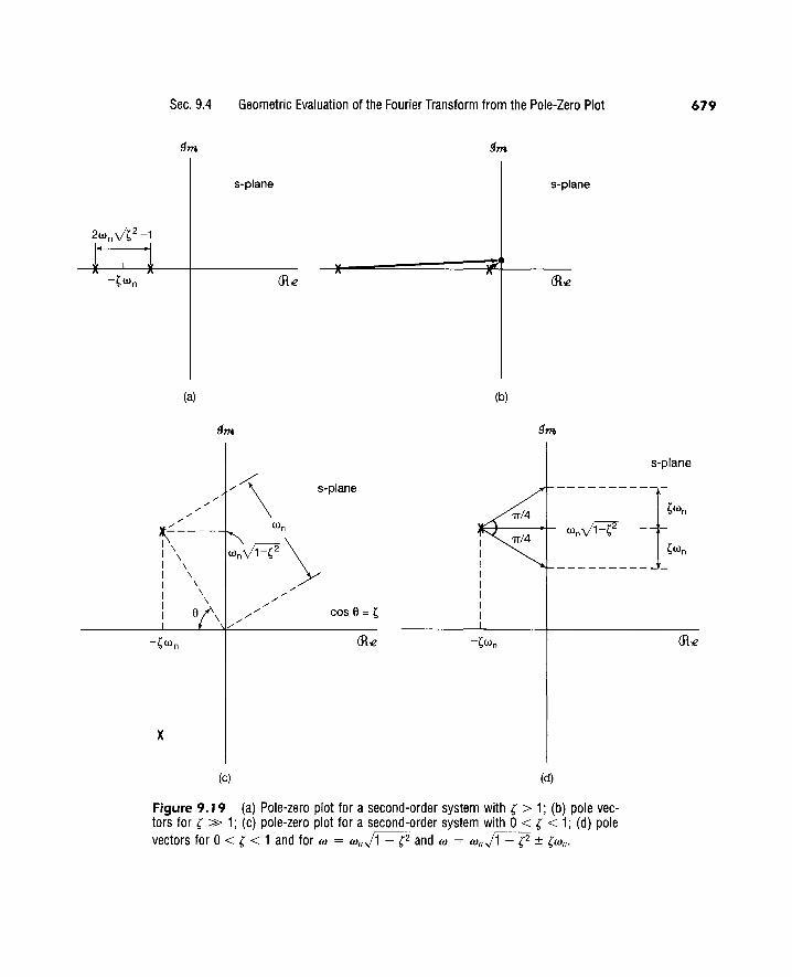
Sec. 9.4 Geometric Evaluation of the Fourier Transform from the Pole-Zero Plot
gm gm
s-plane s-plane
(a) (b)
gm gm
cos e = ~
X
(c) (d)
Figure 9.19 (a) Pole-zero plot for a second-order system with ( > 1; (b) pole vectors for ( >> 1; (c) pole-zero plot for a second-order system with 0 < ( < 1; (d) pole vectors for 0 < ( < 1 and for w = wn~ and w = wn~ :±: (wn.
679
s-plane

680 The Laplace Transform Chap.9
particular, the length of that pole vector has a minimum at w = wn~· Thus, qualitatively, we would expect the magnitude of the frequency response to exhibit a peak in the vicinity of that frequency. Because of the presence of the other pole, the peak will occur not exactly at w = Wn~, but at a frequency slightly less than this. A careful sketch of the magnitude of the frequency response is shown in Figure 9.20(a) for w n = 1 and several values of ( where the expected behavior in the vicinity of the poles is clearly evident. This is consistent with our analysis of second-order systems in Section 6.5.2.
JH(jw)l
-1 w
(a)
<l:H(jw)
w
(b)
Figure 9.20 (a) Magnitude and (b) phase of the frequency response for a second-order system with 0 < ~ < 1.

Sec. 9.4 Geometric Evaluation of the Fourier Transform from the Pole-Zero Plot 681
Thus, for 0 < ( < 1, the second-order system is a nonideal bandpass filter, with the parameter ( controlling the sharpness and width of the peak in the frequency response. In particular, from the geometry in Figure 9 .19( d), we see that the length of the pole vector from the second-quadrant pole increases by a factor of j2 from its minimum at w = w n ~when w increases or decreases from this value by ( w n. Consequently, for small (,and neglecting the effect of the distant third-quadrant pole, IH(jw )I is within a factor of J2 of its peak value over the frequency range
Wn~- (wn < W < Wn~ + (wn.
If we define the relative bandwidth Bas the length of this frequency interval divided by the undamped natural frequency w n, we see that
B = 2(.
Thus, the closer ( is to zero, the sharper and narrower the peak in the frequency response is. Note also that B is the reciprocal of the quality measure Q for second-order systems defined in Section 6.5.2. Thus, as the quality increases, the relative bandwidth decreases and the filter becomes increasingly frequency selective.
An analogous picture can be developed for <r:H ( w ), which is plotted in Figure 9 .20(b) for wn = 1 and several values of(. As can be seen from Figure 9.19(d), the angle of the second-quadrant pole vector changes from -11'14 to 0 to 11'14 as w changes from Wn~- (wn toWn~ toWn~+ (wn. For small values of(, the angle for the third-quadrant pole changes very little over this frequency interval, resulting in a rapid change in <r:H(jw) of approximately 71'/2 over the interval, as captured in the figure.
Varying wn with ( fixed only changes the frequency scale in the preceding discussion-i.e., IH(w)l and <r:H(w) depend only on wlwn. From Figure 9.19(c), we also can readily determine how the poles and system characteristics change as we vary (, keeping w n constant. Since cos (} = (, the poles move along a semicircle with fixed radius w n. For ( = 0, the two poles are on the imaginary axis. Correspondingly, in the time domain, the impulse response is sinusoidal with no damping. As ( increases from 0 to 1, the two poles remain complex and move into the left-half plane, and the vectors from the origin to the poles maintain a constant overall magnitude w n. As the real part of the poles becomes more negative, the associated time response will decay more quickly as t ~ oo. Also, as we have seen, as (increases from 0 toward 1, the relative bandwidth of the frequency response increases, and the frequency response becomes less sharp and less frequency selective.
9.4.3 All-Pass Systems
As a final illustration of the geometric evaluation of the frequency response, let us consider a system for which the Laplace transform of the impulse response has the pole-zero plot shown in Figure 9.21(a). From this figure, it is evident that for any point along the jw-axis, the pole and zero vectors have equal length, and consequently, the magnitude of the frequency response is constant and independent of frequency. Such a system is com-

682 The Laplace Transform
s-plane
w
-a a
(a)
<tH(jw)
IH(jw)l
w
(b)
Figure 9.21 (a) Pole-zero plot for an all-pass system; (b) magnitude and phase of an all-pass frequency response.
Chap.9
monly referred to as an all-pass system, since it passes all frequencies with equal gain (or attenuation). The phase of the frequency response is 8 I - 82, or, since 8 I = 7T - 82,
1:H(jw) = 7T- 282. (9.80)
From Figure 9.21(a), 82 = tan- 1 (wla), and thus,
-1-H(jw) = 7r- 2tan- 1 (~). (9.81)
The magnitude and phase of H(jw) are illustrated in Figure 9.2l(b).
9.5 PROPERTIES OF THE LAPLACE TRANSFORM
In exploiting the Fourier transform, we relied heavily on the set of properties developed in Section 4.3. In the current section, we consider the corresponding set of properties for

Sec. 9.5 Properties of the Laplace Transform 683
the Laplace transform. The derivations of many of these results are analogous to those of the corresponding properties for the Fourier transform. Consequently, we will not present the derivations in detail, some of which are left as exercises at the end of the chapter. (See Problems 9.52-9.54.)
9.5.1 Linearity of the laplace Transform
If
and
then
with a region of convergence that will be denoted as R1
x2(s) with a region of convergence that
will be denoted as R2,
£ ax1 (t) + bx2(t) ~ aX1 (s) + bX2(s), with ROC
containing R 1 n R 2. (9.82)
As indicated, the region of convergence of X(s) is at least the intersection of R1 and R2,
which could be empty, in which case X(s) has no region of convergence-i.e., x(t) has no Laplace transform. For example, for x(t) as in eq. (9.47) of Example 9.7, with b > 0 the ROC for X(s) is the intersection of the ROCs for the two terms in the sum. If b < 0, there are no common points in R1 and R2 ; that is, the intersection is empty, and thus, x(t) has no Laplace transform. The ROC can also be larger than the intersection. As a simple example, for x1 (t) = x2(t) and a = -bin eq. (9.82), x(t) = 0, and thus, X(s) = 0. The ROC of X(s) is then the entire s-plane.
The ROC associated with a linear combination of terms can always be constructed by using the properties of the ROC developed in Section 9 .2. Specifically, from the intersection of the ROCs for the individual terms (assuming that it is not empty), we can find a line or strip that is in the ROC of the linear combination. We then extend this to the right ((Re{s} increasing) and to the left (ffi-e{s} decreasing) to the nearest poles (which may be at infinity).
Example 9. 1 3
In this example, we illustrate the fact that the ROC for the Laplace transform of a linear combination of signals can sometimes extend beyond the intersection of the ROCs for the individual terms. Consider
X(t) = Xt (t) - X2(t), (9.83)

684 The Laplace Transform Chap.9
where the Laplace transforms of x 1 (t) and x 2(t) are, respectively,
1 X,(s) = s + 1' CRe{s} > -1, (9.84)
and
1 X2(s) = (s + 1)(s + 2)' CR..e{s} > -1. (9.85)
The pole-zero plot, including the ROCs for X1 (s) and X2(s), is shown in Figures 9.22(a) and (b). From eq. (9.82),
1 1 X(s) = -s -+-1 - -(s_+_1_)-(s_+_2_)
s + 1 (9.86)
(s + l)(s + 2) - s + 2 ·
Thus, in the linear combination of x 1 (t) and x 2(t), the pole at s = -1 is canceled by a zero at s = -1. The pole-zero plot for X(s) = X1 (s)- X2(s) is shown in Figure 9.22(c). The intersection of the ROCs for X1 (s) and X2(s) is ffi-e{s} > -1. However, since the ROC is always bounded by a pole or infinity, for this example the ROC for X(s) can be extended to the left to be bounded by the pole at s = -2, as a result of the pole-zero cancellation at s = - 1.
!1m !1m !1m
I I I I s-plane I s-plane I I
R1 I
f\ I R I I I
I I I I I I
-~ -X-X -~ ffi-e -2 -1 ffi-e I I I I I I I I I I I I I I I
(a) (b) (c)
Figure 9.22 Pole-zero plots and ROCs for Example 9.13: (a) X1(s); (b) X2(s); (c) X1 (s) - X2(s). The ROC for X1 (s) - X2(s) includes the intersection of R1 and R2, which can then be extended to be bounded by the pole at s = -2.
s-plane
ffi-e
9.5.2 Time Shifting
If
.c x(t) ~ X(s), withROC = R,
then
.c x(t- to) ~ e-stox(s), with ROC = R. (9.87)

Sec. 9.5 Properties of the Laplace Transform
9.5.3 Shifting in the s-Domain
If
£ x(t) ~ X(s),
then
with ROC= R,
£ esot x(t) ~ X(s - s0), with ROC = R + CRe{so}.
685
(9.88)
That is, the ROC associated with X(s- s0) is that of X(s), shifted by CRe{s0}. Thus, for any values that is in R, the values + CR.e{s0} will be in R1. This is illustrated in Figure 9.23. Note that if X(s) has a pole or zero at s = a, thenX(s-s0) has a pole or zero ats-s0 = ai.e., s = a + so.
An important special case of eq. (9.88) is when s0 = jw0-i.e., when a signal x(t) is used to modulate a periodic complex exponential ejwot. In this case, eq. (9.88) becomes
. £ eJwot x(t) ~ X(s - jw0 ), with ROC = R. (9.89)
The right-hand side of eq. (9.89) can be interpreted as a shift in the s-plane parallel to the jw-axis. That is, if the Laplace transform of x(t) has a pole or zero at s = a, then the Laplace transform of ejwot x(t) has a pole or zero at s = a+ jw0 .
9.5.4 Time Scaling
If
l
£ x(t) ~ X(s),
1 s-plane
Rl I I
l r1 I I l I I 1
(a)
withROC = R,
I I
r2 + CR-e (so) I I I I I
(b)
I I s-plane I I I l
Figure 9.23 Effect on the ROC of shifting in the s-domain: (a) the ROC of X(s); (b) the ROC of X(s- s0).

686 The Laplace Transform Chap.9
then
x(at) ....:.._. 1!
1x(n with ROC R1 ~ aR. (9.90)
That is, for any value s in R [which is illustrated in Figure 9.24(a)], the value a/s will be in Rt. as illustrated in Figure 9.24(b) for a positive value of a < 1. Note that, for 0 <a< 1, there is a compression in the size of the ROC of X(s) by a factor of a, as depicted in Figure 9.24(b), while for a> 1, the ROC is expanded by a factor of a. Also, eq. (9.90) implies that if a is negative, the ROC undergoes a reversal plus a scaling. In particular, as depicted in Figure 9.24(c), the ROC of lliaiX(sla) for 0 >a > -1 involves
s-plane
R
(a)
9m
~ ~ a a
(c)
.!1 a
(b)
s-plane
s-plane
~ a
Figure 9.24 Effect on the ROC of time scaling: (a) ROC of X(s); (b) ROC of (1/lai}X(s/a) for 0 <a< 1; (c) ROC of (1/lai}X(s/a) for 0 >a> -1.

Sec. 9.5 Properties of the Laplace Transform 687
a reversal about the jw-axis, together with a change in the size of the ROC by a factor of lal· Thus, time reversal of x(t) results in a reversal of the ROC. That is,
9.5.5 Conjugation
If
then
Therefore,
£ x(-t) ~ X(-s), with ROC= -R.
£ x(t) ~ X(s), with ROC = R,
* £ * * x (t) ~ X (s ), with ROC = R.
X(s) = X*(s*) when x(t) is real.
(9.91)
(9.92)
(9.93)
(9.94)
Consequently, if x(t) is real and if X(s) has a pole or zero at s = s0 (i.e., if X(s) is unbounded or zero at s = s0), then X(s) also has a pole or zero at the complex conjugate points = s~. For example, the transform X(s) for the real signal x(t) in Example 9.4 has poles at s = 1 ± 3j and zeros at s = ( -5 ± .ifil)/2.
9. 5. 6 Convolution Property
If
and
then
with ROC = R1,
with ROC = R2,
(9.95)
In a manner similar to the linearity property set forth in Section 9.5.1, the ROC of X1 (s)X2(s) includes the intersection of the ROCs of X1 (s) and X2(s) and may be larger if pole-zero cancellation occurs in the product. For example, if
s + 1 XJ(S) = s + 2' CR-t:?{s} > -2, (9.96)

688
and
s+2 X2(s) = s + 1,
The Laplace Transform
CRe{s} > -1,
then X1 (s)X2(s) = 1, and its ROC is the entire s-plane.
Chap. 9
(9.97)
As we saw in Chapter 4, the convolution property in the context of the Fourier transform plays an important role in the analysis of linear time-invariant systems. In Sections 9.7 and 9.8 we will exploit in some detail the convolution property for Laplace transforms for the analysis of LTI systems in general and, more specifically, for the class of systems represented by linear constant-coefficient differential equations.
9.5.7 Differentiation in the Time Domain
If
then
dx(t)
dt
£ x(t) ~ X(s),
£ ~ sX(s),
with ROC= R,
with ROC containing R. (9.98)
This property follows by differentiating both sides of the inverse Laplace transform as expressed in equation (9.56). Specifically, let
1 f<T+ jx x(t) = -. X(s)est ds.
21T 1 (T- joo
Then
dx(t) 1 J<T+joo -- - -
2 . sX(s)e5tds.
dt 1T 1 (T- joo (9.99)
Consequently, dx(t)ldt is the inverse Laplace transform of sX(s). The ROC of sX(s) includes the ROC of X(s) and may be larger if X(s) has a first-order pole at s = 0 that is canceled by the multiplication by s. For example, if x(t) = u(t), then X(s) = 1/s, with an ROC that is CRe{s} > 0. The derivative of x(t) is an impulse with an associated Laplace transform that is unity and an ROC that is the entire s-plane.
9.5.8 Differentiation in the s-Domain
Differentiating both sides of the Laplace transform equation (9.3), i.e.,
we obtain
X(s) ~ r~x x(t)e-"dt,
dX(s) ds r
+oo
-oo (-t)x(t)e-stdt.

Sec. 9.5 Properties of the Laplace Transform
Consequently, if
£ x(t) ~ X(s), with ROC= R,
then
£ dX(s) -tx(t) ~
' withROC = R.
ds
The next two examples illustrate the use of this property.
Example 9.14
Let us find the Laplace transform of
x(t) = te-at u(t).
Since
s +a' CRe{s} > -a,
it follows from eq. (9.100) that
te-atu(t) ~ _!!__ [-1-] = __ 1_, . ds s +a (s + a)2
CRe{s} >-a.
In fact, by repeated application of eq. (9.100), we obtain
t2 -e-at u(t) 2
£ 1 ~---
(s+a)3' CRe{s} >-a,
and, more generally,
tn-I
(n- 1)! e-at u(t) (s+a)n' ffi-e{s} > -a.
689
(9.100)
(9.101)
(9.102)
(9.103)
(9.104)
As the next example illustrates, this specific Laplace transform pair is particularly useful when applying partial-fraction expansion to the determination of the inverse Laplace transform of a rational function with multiple-order poles.
Example 9. 1 5
Consider the Laplace transform
2s2 + 5s + 5 X(s) = (s + 1)2(s + 2)' ffi-e{s} > -1.
Applying the partial-fraction expansion method described in the appendix, we can write
2 1 3 X(s) = (s + 1)2 - (s + 1) + s + 2' ffi-e{s} > -1. (9.105)

690 The Laplace Transform Chap.9
Since the ROC is to the right of the poles at s = -1 and -2, the inverse transform of each of the terms is a right-sided signal, and, applying eqs. (9.14) and (9.104), we obtain the inverse transform
9.5.9 Integration in the Time Domain
If £
x(t) ~ X(s), with ROC= R,
then
L x(T)dT 1 -X(s), with ROC containing s R n {(Re{s} > 0}.
(9.106)
This property is the inverse of the differentiation property set forth in Section 9.5. 7. It can be derived using the convolution property presented in Section 9.5.6. Specifically,
fx x( T)dT = u(t) * x(t). (9.107)
From Example 9.1, with a = 0,
u(t) £ ~
s'
and thus, from the convolution property,
£ u(t) * x(t) ~
ffi-e{s} > 0,
1 -X(s), s
(9.108)
(9.109)
with an ROC that contains the intersection of the ROC of X(s) and the ROC of the Laplace transform of u(t) in eq. (9.108), which results in the ROC given in eq. (9.106).
9.5.1 0 The Initial- and Final-Value Theorems
Under the specific constraints that x(t) = 0 for t < 0 and that x(t) contains no impulses or higher order singularities at the origin, one can directly calculate, from the Laplace transform, the initial value x(O+)-i.e., x(t) as t approaches zero from positive values of t. Specifically the initial-value theorem states that
x(O+) = lim sX(s), (9.110) s~x
Also, if x(t) = 0 fort< 0 and, in addition, x(t) has a finite limit as t ~ x, then the final-
value theorem says that lim x(t) = lim sX(s). (9.111) t---+x s---->0
The derivation of these results is considered in Problem 9.53.

Sec. 9.5 Properties of the Laplace Transform 691
Example 9.16
The initial- and final-value theorems can be useful in checking the correctness of the Laplace transform calculations for a signal. For example, consider the signal x(t) in Example 9.4. From eq. (9.24), we see that x(O+) = 2. Also, using eq. (9.29), we find that
. . 2s3 + 5s2 + 12s hm sX(s) = hm
3 4 2 14 20 = 2,
S->OC S-->00 S + S + S +
which is consistent with the initial-value theorem in eq. (9.110).
9.5.11 Table of Properties
In Table 9.1, we summarize the properties developed in this section. In Section 9. 7, many of these properties are used in applying the Laplace transform to the analysis and characterization of linear time-invariant systems. As we have illustrated in several examples, the various properties of Laplace transforms and their ROCs can provide us with
TABLE 9.1 PROPERTIES OF THE LAPLACE TRANSFORM
Laplace Section Property Signal Transform ROC
x(t) X(s) R x, (t) X1(s) R, x2(t) X2(s) R2
---------- ----------- ------------------9.5.1 Linearity ax1 (t) + bx2(t) aX1 (s) + bX2(s) At least R1 n R2 9.5.2 Time shifting x(t- to) e-sto X(s) R 9.5.3 Shifting in the s-Domain esot x(t) X(s- s0 ) Shifted version of R (i.e., s is
in the ROC if s - s0 is in R)
x(at) 1 x(s) Scaled ROC (i.e., s is in the Ia! a ROC if s/a is in R) 9.5.4 Time scaling
9.5.5 Conjugation x*(t) X*(s*) R 9.5.6 Convolution x 1 (t) * x2(t) X1(s)X2(s) At least R1 n R2
d At least R dix(t) sX(s) 9.5. 7 Differentiation in the
Time Domain
-tx(t) d dsX(s) R 9.5.8 Differentiation in the
s-Domain
foo X(T)d(T) 1
At least R n {<Re{s} > 0} -X(s) s
9.5.9 Integration in the Time Domain
Initial- and Final-Value Theorems 9.5.1 0 If x(t) = 0 for t < 0 and x(t) contains no impulses or higher-order singularities at t = 0, then
x(O+) = lim sX(s) s~oo
If x(t) = 0 fort< 0 and x(t) has a finite limit as t -7 oc, then lim x(t) = lim sX(s)
1-+-:xo S--t-:xo

692 The Laplace Transform Chap.9
considerable information about a signal and its transform that can be useful either in characterizing the signal or in checking a calculation. In Sections 9.7 and 9.8 and in some of the problems at the end of this chapter, we give several other examples of the uses of these properties.
9.6 SOME LAPLACE TRANSFORM PAIRS
As we indicated in Section 9.3, the inverse Laplace transform can often be easily evaluated by decomposing X (s) into a linear combination of simpler terms, the inverse transform of each of which can be recognized. Listed in Table 9.2 are a number of useful Laplace
TABLE 9.2 LAPLACE TRANSFORMS OF ELEMENTARY FUNCTIONS
Transform pair Signal Transform ROC
1 8(t) 1 Ails
2 u(t) 1
ffi-c{s} > 0 -
s
3 -u( -t) 1
ffi-c{s} < 0 -s
4 rn-1 1
ffi-c{s} > 0 (n- 1)! u(t) -sn
5 fn-1 1
ffi-c{s} < 0 - (n- 1)! u(-t) -sn
6 e-at u(t) 1 ffi-c{s} > -a --
s+a
7 -e-a1u(-t) 1
ffi-c{s} < -a --s+a
fn-1 1 ffi-c{s} > -a 8 (n- 1)! e-atu(t) ---
(s + a)n
9 fn-1 1
ffi-c{s} < -a -at ( ) - (n _ 1)! e u -t ---(s + a)n
10 8(t- T) e-sT Ails
11 [cosw0 t]u(t) s
ffi-c{s} > 0 --s2 + w5
12 [sin w0 t]u(t) Wo
ffi-c{s} > 0 s2 + w5
13 [e-at coswot]u(t) s+a
ffi-c{s} > -a (s+a)2 +w5
14 [e-at sinwot]u(t) wo ffi-c{s} > -a
(s+a)2 +w5
15 u (t) = dno(t) n dtn
sn All s
16 U-n(t) = u(t) * · · · * u(t) 1
ffi-c{s} > 0 -
'--.r----1 sn
n times
Sec. 9.7 Analysis And Characterization of LTI Systems Using the Laplace Transform 693
transform pairs. Transform pair 1 follows directly from eq. (9.3). Transform pairs 2 and 6 follow directly from Example 9.1 with a = 0 and a = a, respectively. Transform pair 4 was developed in Example 9.14 using the differentiation property. Transform pair 8 follows from transform pair 4 using the property set forth in Section 9.5.3. Transform pairs 3, 5, 7, and 9 are based on transform pairs 2, 4, 6 and 8, respectively, together with the timescaling property of section 9.5.4 with a = -1. Similarly, transform pairs 10 through 16 can all be obtained from earlier ones in the table using appropriate properties in Table 9.1 (see Problem 9.55).
9.7 ANALYSIS AND CHARACTERIZATION OF LTI SYSTEMS USING THE LAPLACE TRANSFORM
One of the important applications of the Laplace transform is in the analysis and characterization of LTI systems. Its role for this class of systems stems directly from the convolution property (Section 9.5.6). Specifically, the Laplace transforms of the input and output of an LTI system are related through multiplication by the Laplace transform of the impulse response of the system. Thus,
Y(s) = H(s )X(s ). (9.112)
where X(s), Y(s), and H(s) are the Laplace transforms of the input, output, and impulse response of the system, respectively. Equation (9 .112) is the counterpart, in the context of Laplace transforms, of eq. (4.56) for Fourier transform. Also, from our discussion in Section 3.2 on the response of LTI systems to complex exponentials, if the input to an LTI system is x(t) = es1
, with sin the ROC of H(s), then the output will be H(s)est; i.e., est is an eigenfunction of the system with eigenvalue equal to the Laplace transform of the impulse response.
If the ROC of H(s) includes the imaginary axis, then for s = jw, H(s) is the frequency response of the LTI system. In the broader context of the Laplace transform, H(s) is commonly referred to as the system function or, alternatively, the transfer function. Many properties of LTI systems can be closely associated with the characteristics of the system function in the s-plane. We illustrate this next by examining several important properties and classes of systems.
9. 7. 1 Causality
For a causal LTI system, the impulse response is zero for t < 0 and thus is right sided. Consequently, from the discussion in Section 9.2, we see that
The ROC associated with the system function for a causal system is a right-half plane.
It should be stressed, however, that the converse of this statement is not necessarily true. That is, as illustrated in Example 9.19 to follow, an ROC to the right of the rightmost

694 The Laplace Transform Chap.9
pole does not guarantee that a system is causal; rather, it guarantees only that the impulse response is right sided. However, if H (s) is rational, then, as illustrated in Examples 9.17 and 9.18 to follow, we can determine whether the system is causal simply by checking to see if its ROC is a right-half plane. Specifically,
For a system with a rational system function, causality of the system is equivalent to the ROC being the right-half plane to the right of the rightmost pole.
Example 9. 1 7
Consider a system with impulse response
h(t) = e-tu(t). (9.113)
Since h(t) = 0 fort < 0, this system is causal. Also, the system function can be obtained from Example 9.1:
H(s) = s + 1' CRe{s} > -1. (9.114)
In this case, the system function is rational and the ROC in eq. (9 .114) is to the right of the rightmost pole, consistent with our statement that causality for systems with rational system functions is equivalent to the ROC being to the right of the rightmost pole.
Example 9. 1 8
Consider a system with impulse response
Since h(t) =I= 0 fort < 0, this system is not causal. Also, from Example 9.7, the system function is
-2 H(s) = s
2 _
1, -1 < CRe{s} < +1.
Thus, H(s) is rational and has an ROC that is not to the right of the the rightmost pole, consistent with the fact that the system is not causal.
Example 9.19
Consider the system function
es H(s) = s + 1' CRe{s} > -1. (9.115)
For this system, the ROC is to the right of the rightmost pole. Therefore, the impulse response must be right sided. To determine the impulse response, we first use the result

Sec. 9.7 Analysis And Characterization of LTI Systems Using the Laplace Transform 695
of Example 9.1:
e-r u(t) s + 1'
CRe{s} > -1. (9.116)
Next, from the time-shifting property of Section 9.5.2 [eq. (9.87)], the factor e' in eq. (9.115) can be accounted for by a shift in the time function in eq. (9.116). Then
CRe{s} > -1, (9.117)
so that the impulse response associated with the system is
h(t) = e-u+ 1 )u(t + 1), (9.118)
which is nonzero for - 1 < t < 0. Hence, the system is not causal. This example serves as a reminder that causality implies that the ROC is to the right of the rightmost pole, but the converse is not in general true, unless the system function is rational.
In an exactly analogous manner, we can deal with the concept of anticausality. A system is anticausal if its impulse response h(t) = 0 for t > 0. Since in that case h(t) would be left sided, we know from Section 9.2 that the ROC of the system function H(s) would have to be a left-half plane. Again, in general, the converse is not true. That is, if the ROC of H(s) is a left-half plane, all we know is that h(t) is left sided. However, if H(s) is rational, then having an ROC to the left of the leftmost pole is equivalent to the system being anticausal.
9.7.2 Stability
The ROC of H(s) can also be related to the stability of a system. As mentioned in Section 2.3.7, the stability of an LTI system is equivalent to its impulse response being absolutely integrable, in which case (Section 4.4) the Fourier transform ofthe impulse response converges. Since the Fourier transform of a signal equals the Laplace transform evaluated along the jw-axis, we have the following:
An LTI system is stable if and only if the ROC of its system function H(s) includes the entire jw-axis [i.e., ~e(s) = 0].
Example 9.20
Let us consider an LTI system with system function
s - 1 H (s) = -(s_+_1 )-(s---2-) (9.119)
Since the ROC has not been specified, we know from our discussion in Section 9.2 that there are several different ROCs and, consequently, several different system impulse responses that can be associated with the algebraic expression for H(s) given in eq. (9.119).

696 The Laplace Transform Chap.9
If, however. we have information about the causality or stability of the system, the appropriate ROC can be identified. For example, if the system is known to be causal, the ROC will be that indicated in Figure 9.25(a), with impulse response
(2 1 ,., ) lz(t) = 3 e r + 3 e-r u(t). (9.120)
Note that this particular choice of ROC does not include the jw-axis, and consequently, the corresponding system is unstable (as can be checked by observing that h(t) is not absolutely integrable). On the other hand, if the system is known to be stable, the ROC is that given in Figure 9.25(b). and the corresponding impulse response is
2 . 1 ,., lz(t) = -e -ru(t)- -
3e-1u(-t),
3
which is absolutely integrable. Finally, for the ROC in Figure 9.25(c), the system is anticausal and unstable, with
9m 9m
I I I s-plane I s-plane I
I I I I I I I I
X X X X -1 2 <R-c -1 2
I I I
I I I I I I I I I I I I I I I
(a) (b)
9m
I I s-plane I I I I x X ~1 2 <R-c
(c)
Figure 9.25 Possible ROCs for the system function of Example 9.20 with poles at s = -1 and s = 2 and a zero at s = 1: (a) causal, unstable system; (b) noncausal, stable system; (c) anticausal, unstable system.
<R-c

Sec. 9.7 Analysis And Characterization of LTI Systems Using the Laplace Transform 697
It is perfectly possible, of course, for a system to be stable (or unstable) and have a system function that is not rational. For example, the system function in eq. (9.115) is not rational, and its impulse response in eq. (9 .118) is absolutely integrable, indicating that the system is stable. However, for systems with rational system functions, stability is easily interpreted in terms of the poles of the system. For example, for the pole-zero plot in Figure 9.25, stability corresponds to the choice of an ROC that is between the two poles, so that the jw-axis is contained in the ROC.
For one particular and very important class of systems, stability can be characterized very simply in terms of the locations of the poles. Specifically, consider a causal LTI system with a rational system function H(s). Since the system is causal, the ROC is to the right of the rightmost pole. Consequently, for this system to be stable (i.e., for the ROC to include the jw-axis), the rightmost pole of H(s) must be to the left of the jw-axis. That is,
A causal system with rational system function H(s) is stable if and only if all of the poles of H(s) lie in the left-half of the s-plane-i.e., all of the poles have negative real parts.
Example 9.21
Consider again the causal system in Example 9.17. The impulse response in eq. (9 .113) is absolutely integrable, and thus the system is stable. Consistent with this, we see that the pole of H(s) in eq. (9.114) is at s = -1, which is in the left-half of the s-plane. In contrast, the causal system with impulse response
h(t) = e21 u(t)
is unstable, since h(t) is not absolutely integrable. Also, in this case
1 H(s) = --,
s-2 ffi-R{s} > 2,
so the system has a pole at s = 2 in the right half of the s-plane.
Example 9.22
Let us consider the class of causal second-order systems previously discussed in Sections 9.4.2 and 6.5.2. The impulse response and system function are, respectively,
and
where
CJ = -~wn +wn~•
C2 = -~wn - Wn~' M = Wn
2~·
(9.121)
(9.122)
(9.123)
(9.124)
(9.125)

698
9m
I I I I I
~ I I I I I I I
The Laplace Transform
s-plane
Figure 9.26 Pole locations and ROC for a causal second-order system with?< 0.
Chap. 9
In Figure 9.19, we illustrated the pole locations for ( > 0. In Figure 9.26, we illustrate the pole locations for ( < 0. As is evident from the latter figure and from eqs. (9.124) and (9.125), for ( < 0 both poles have positive real parts. Consequently, for ( < 0, the causal second-order system cannot be stable. This is also evident in eq. (9.121), since, with (Jl.e{c 1} > 0 and <Re{c2} > 0, each term grows exponentially as t increases, and thus h(t) cannot be absolutely integrable.
9. 7.3 LTI Systems Characterized by Linear Constant-Coefficient
Differential Equations
In Section 4. 7, we discussed the use of the Fourier transform to obtain the frequency response of an LTI system characterized by a linear constant -coefficient differential equation without first obtaining the impulse response or time-domain solution. In an exactly analogous manner, the properties of the Laplace transform can be exploited to directly obtain the system function for an LTI system characterized by a linear constant-coefficient differential equation. We illustrate this procedure in the next example.
Example 9.23
Consider an LTI system for which the input x(t) and output y(t) satisfy the linear constant -coefficient differential equation
dy(t) -----;[( + 3y(t) = x(t). (9.126)

Sec. 9.7 Analysis and Characterization of LTI Systems Using the Laplace Transform 699
Applying the Laplace transform to both sides of eq. (9.126), and using the linearity and differentiation properties set forth in Sections 9.5.1 and 9.5.7, respectively [(eqs. (9.82) and (9.98)], we obtain the algebraic equation
sY(s) + 3Y(s) = X(s). (9.127)
Since, from eq. (9.112), the system function is
H( ) = Y(s) s X(s)'
we obtain, for this system,
H(s) = s + 3" (9.128)
This, then, provides the algebraic expression for the system function, but not the region of convergence. In fact, as we discussed in Section 2.4, the differential equation itself is not a complete specification of the LTI system, and there are, in general, different impulse responses, all consistent with the differential equation. If, in addition to the differential equation, we know that the system is causal, then the ROC can be inferred to be to the right of the rightmost pole, which in this case corresponds to CRe{s} > -3. If the system were known to be anticausal, then the ROC associated with H(s) would be (Jl.e{s} < -3. The corresponding impulse response in the causal case is
h(t) = e-3r u(t), (9.129)
whereas in the anticausal case it is
h(t) = -e-3t u( -t). (9.130)
The same procedure used to obtain H (s) from the differential equation in Example 9.23 can be applied more generally. Consider a general linear constant-coefficient differential equation of the form
~ dky(t) _ ~ b dk x(t) Lak-dk - L k-dk · k=O t k=O t
(9.131)
Applying the Laplace transform to both sides and using the linearity and differentiation properties repeatedly, we obtain
(9.132)
or
H(s) = (9.133)
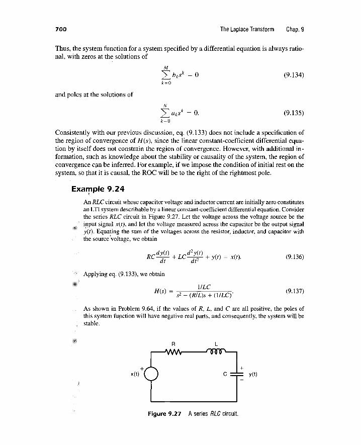
700 The Laplace Transform Chap.9
Thus, the system function for a system specified by a differential equation is always rational, with zeros at the solutions of
(9.134)
and poles at the solutions of
(9.135)
Consistently with our previous discussion, eq. (9.133) does not include a specification of the region of convergence of H(s), since the linear constant-coefficient differential equation by itself does not constrain the region of convergence. However, with additional information, such as know ledge about the stability or causality of the system, the region of convergtmce can be inferred. For example, if we impose the condition of initial rest on the system, so that it is causal, the ROC will be to the right of the rightmost pole.
Example 9.24 t
An RLC circuit whose capacitor voltage and inductor current are initially zero constitutes an LTI system describable by a linear constant-coefficient differential equation. Consider the series RLC circuit in Figure 9.27. Let the voltage across the voltage source be the input signal x(t), and let the voltage measured across the capacitor be the output signal y(t). Equating the sum of the voltages across the resistor, inductor, and capacitor with the source 'voltage, we obtain
Rc dy(t) LCd2y(t) () = ()
dt + dt2 + y t X t .
Applying eq. (9.133), we obtain
l!LC H(s) = s2 + (RIL)s + (1/LC)'
(9.136)
(9.137)
As shown in Problem 9.64, if the values of R, L, and C are all positive, the poles of this system fupction will have negative real parts, and consequently, the system will be stable.
R L
Figure 9.27 A series RLC circuit.

Sec. 9.7 Analysis and Characterization of LTI Systems Using the Laplace Transform 701
9.7.4 Examples Relating System Behavior to the System Function
As we have seen, system properties such as causality and stability can be directly related to the system function and its characteristics. In fact, each of the properties of Laplace transforms that we have described can be used in this way to relate the behavior of the system to the system function. In this section, we give several examples illustrating this.
Example 9.25
Suppose we know that if the input to an LTI system is
x(t) = e-3' u(t),
then the output is
As we now show, from this knowledge we can determine the system function for this system and from this can immediately deduce a number of other properties of the system.
and
Taking Laplace transforms of x(t) and y(t), we get
1 X(s) = --
3,
s+
1 Y(s) = (s + l)(s + 2)'
ffi-e{s} > -3,
ffi-e{s} > -1.
From eq. (9.112), we can then conclude that
H(s) = Y(s) = s + 3 X(s) (s + l)(s + 2)
s+3 s2 + 3s + 2·
Furthermore, we can also determine the ROC for this system. In particular, we know from the convolution property set forth in Section 9.5.6 that the ROC of Y(s) must include at least the intersections of the ROCs of X(s) and H(s). Examining the three possible choices for the ROC of H(s) (i.e., to the left of the pole at s = -2, between the poles at -2 and -1, and to the right of the pole at s = -1), we see that the only choice that is consistent with the ROCs of X(s) and Y(s) is ffi-e{s} > -1. Since this is to the right of the rightmost pole of H (s ), we conclude that H (s) is causal, and since both poles of H(s) have negative real parts, it follows that the system is stable. Moreover, from the relationship between eqs. (9.131) and (9.133), we can specify the differential equation that, together with the condition of initial rest, characterizes the system:
d 2y(t) 3
dy(t) 2 () _ dx(t) 3 () d ? + d + yt- d + xt. t- t t
Example 9.26
Suppose that we are given the following information about an LTI system:
1. The system is causal.
2. The system function is rational and has only two poles, at s = -2 and s = 4.

702 The Laplace Transform Chap.9
3. If x(t) = 1, then y(t) = 0.
4. The value of the impulse response at t = o+ is 4.
From this information we would like to determine the system function of the system. From the first two facts, we know that the system is unstable (since it is causal and
has a pole at s = 4 with positive real part) and that the system function is of the form
p(s) H(s) = (s + 2)(s- 4)
p(s)
s2 - 2s- 8'
where p(s) is a polynomial ins. Because the response y(t) to the input x(t) = 1 = e0·r
must equal H(O) · e0'' = H(O), we conclude, from fact 3, that p(O) = 0-i.e., that p(s) must have a root at s = 0 and thus is of the form
p(s) = sq(s),
where q(s) is another polynomial ins. Finally, from fact 4 and the initial-value theorem in Section 9.5.10, we see that
1' H( 1' s2q(s) 4 s~ s s) = s~ s2 - 2s- 8 = · (9.138)
Ass ~ oo, the terms of highest power ins in both the numerator and the denominator of sH(s) dominate and thus are the only ones of importance in evaluating eq. (9.138). Furthermore, if the numerator has higher degree than the denominator, the limit will diverge. Consequently, we can obtain a finite nonzero value for the limit only if the degree of the numerator of sH(s) is the same as the degree of the denominator. Since the degree of the denominator is 2, we conclude that, for eq. (9.138) to hold, q(s) must be a constant-i.e., q(s) = K. We can evaluate this constant by evaluating
Equating eqs. (9.138) and (9.139), we see that K = 4, and thus,
4s H(s) = (s + 2)(s- 4)
Example 9.27
(9.139)
Consider a stable and causal system with impulse response h(t) and system function H(s). Suppose H(s) is rational, contains a pole at s = -2, and does not have a zero at the origin. The location of all other poles and zeros is unknown. For each of the following statements let us determine whether we can definitely say that it is true, whether we can definitely say that it is false, or whether there is insufficient information to ascertain the statement's truth:
(a) ~ { h(t)e3'} converges.
(b) L+: h(t) dt = o. (c) th(t) is the impulse response of a causal and stable system.

Sec. 9.7 Analysis and Characterization of LTI Systems Using the Laplace Transform
(d) d h(t)ldt contains at least one pole in its Laplace transform.
(e) h(t) has finite duration.
(f) H(s) = H( -s).
(g) lim.1 _,x H(s) = 2.
703
Statement (a) is false, since ty{h(t)e3t} corresponds to the value of the Laplace transform of h(t) at s = -3. If this converges, it implies that s = -3 is in the ROC. A causal and stable system must always have its ROC to the right of all of its poles. However, s = -3 is not to the right of the pole at s = -2.
Statement (b) is false, because it is equivalent to stating that H(O) = 0. This contradicts the fact that H(s) does not have a zero at the origin.
Statement (c) is true. According to Table 9.1, the property set forth in Section 9.5.8, the Laplace transform of th(t) has the same ROC as that of H(s). This ROC includes the jw-axis, and therefore, the corresponding system is stable. Also, h(t) = 0 fort < 0 implies that th(t) = 0 fort < 0. Thus, th(t) represents the impulse response of a causal system.
Statement (d) is true. According to Table 9.1, dh(t)ldt has the Laplace transform sH(s). The multiplication by s does not eliminate the pole at s = -2.
Statement (e) is false. If h(t) is of finite duration, then if its Laplace transform has any points in its ROC, the ROC must be the entire s-plane. However, this is not consistent with H(s) having a pole at s = -2.
Statement (f) is false. If it were true, then, since H(s) has a pole at s = -2, it must also have a pole at s = 2. This is inconsistent with the fact that all the poles of a causal and stable system must be in the left half of the s-plane.
The truth of statement (g) cannot be ascertained with the information given. The statement requires that the degree of the numerator and denominator of H(s) be equal, and we have insufficient information about H(s) to determine whether this is the case.
9. 7. 5 Butterworth Filters
In Example 6.3 we briefly introduced the widely-used class of LTI systems known as Butterworth filters. The filters in this class have a number of properties, including the characteristics of the magnitude of the frequency response of each of these filters in the passband, that make them attractive for practical implementation. As a further illustration of the usefulness of Laplace transforms, in this section we use Laplace transform techniques to determine the system function of a Butterworth filter from the specification of its frequency response magnitude.
An Nth-order lowpass Butterworth filter has a frequency response the square of whose magnitude is given by
1 + (jwl jwc)2N' (9.140)
where N is the order of the filter. From eq. (9.140), we would like to determine the system function B(s) that gives rise to IB(Jw )1 2. We first note that, by definition,
IB(Jw )1 2 = B(jw )B*(jw ). (9.141)

704 The Laplace Transform Chap.9
If we restrict the impulse response of the Butterworth filter to be real, then from the property of conjugate symmetry for Fourier transforms,
B*(jw) = B(- jw),
so that
1 B(jw )B(- jw) = 1 + (jwl jwc)2N.
Next, we note that B(s)ls=jw = B(jw), and consequently, from eq. (9.143),
1 B(s)B( -s) = 1 ( I . )2N. + S ]We
(9.142)
(9.143)
(9.144)
The roots of the denominator polynomial corresponding to the combined poles of B(s)B( -s) are at
s = ( -1)112N (jwc).
Equation (9 .145) is satisfied for any value s = s P for which
lspl = We
and
7T(2k + 1) 7T <.sp = 2N + 2' k an integer;
that is,
(. [7T(2k + 1) ]) s P = w c exp 1
2N + 7T 12 .
(9.145)
(9.146)
(9.147)
(9.148)
In Figure 9.28 we illustrate the positions of the poles of B(s)B( -s) for N 1, 2, 3, and 6. In general, the following observations can be made about these poles:
1. There are 2N poles equally spaced in angle on a circle of radius We in the s-plane.
2. A pole never lies on the jw-axis and occurs on the 0'-axis for N odd, but not for N even.
3. The angular spacing between the poles of B(s)B( -s) is 7T/N radians.
To determine the poles of B(s) given the poles of B(s)B( -s), we observe that the poles of B(s)B( -s) occur in pairs, so that if there is a pole at s = sp, then there is also a pole at s = -sp. Consequently, to construct B(s), we choose one pole from each pair. If we restrict the system to be stable and causal, then the poles that we associate with B(s) are the poles along the semicircle in the left-half plane. The pole locations specify B(s) only to within a scale factor. However, from eq. (9.144), we see that B2(s)ls=O = 1, or equivalently, from eq. (9 .140), the scale factor is chosen so that the square of the magnitude of the frequency response has unity gain at w = 0.
To illustrate the determination of B(s), let us consider the cases N = 1, N = 2, and N = 3. In Figure 9.28 we showed the poles of B(s)B( -s), as obtained from eq. (9.148).

Sec. 9.7 Analysis and Characterization of LTI Systems Using the Laplace Transform 705
9m
N=1
.... .....
" ' / \ I \
----X X------\ 'W \ I c
' "/ ..... _ ....
9m
Figure 9.28 Position of the poles of B(s)B( -s) for N = 1, 2, 3, and 6.
In Figure 9.29 we show the poles associated with B(s) for each of these values of N. The corresponding transfer functions are:
N = 1: B(s) =
N = 2:
N = 3:
We .
S +We'
(s + wc)(s2 + wcs + w~) w~
(9.149)
(9.150)
(9.151)
Based on the discussion in Section 9.7.3, from B(s) we can determine the associated linear constant-coefficient differential equation. Specifically, for the foregoing three values

706 The Laplace Transform
I I
; ,. iwc /
N=1
--X--+------
N=2
- we\ CRo£ -we\ CRo£
' ' ....
I
x- iwc /
\ X
----*--r----------wc \ CRo£ \
'x_
.. ....
Figure 9.29 Position of the poles of B(s) for N = 1, 2, and 3.
of N, the corresponding differential equations are:
N = 1:
N = 2:
N = 3:
9.8 SYSTEM FUNCTION ALGEBRA AND BLOCK DIAGRAM REPRESENTATIONS
Chap. 9
(9.152)
(9.153)
The use of the Laplace transform allows us to replace time-domain operations such as differentiation, convolution, time shifting, and so on, with algebraic operations. We have already seen many of the benefits of this in terms of analyzing LTI systems, and in this section we take a look at another important use of system function algebra, namely, in analyzing interconnections of LTI systems and synthesizing systems as interconnections of elementary system building blocks.

Sec. 9.8 System Function Algebra and Block Diagram Representations 707
9.8.1 System Functions for Interconnections of LTI Systems
Consider the parallel interconnection of two systems, as shown in Figure 9.30(a). The impulse response of the overall system is
(9.155)
and from the linearity of the Laplace transform,
H(s) = H1 (s) + H2(s). (9.156)
Similarly, the impulse response of the series interconnection in Figure 9 .30(b) is
and the associated system function is
(a)
(b)
(9.157)
(9.158)
Figure 9.30 (a) Parallel interconnection of two LTI systems; (b) series combination of two LTI systems.
The utility of the Laplace transform in representing combinations of linear systems through algebraic operations extends to far more complex interconnections than the simple parallel and series combinations in Figure 9.30. To illustrate this, consider the feedback interconnection of two systems, as indicated in Figure 9 .31. The design, applications, and analysis of such interconnections are treated in detail in Chapter 11. While analysis of the system in the time domain is not particularly simple, determining the overall system function from input x(t) to output y(t) is a straightforward algebraic manipulation. Specifically, from Figure 9.31,
Y(s) = H 1 (s)E(s),
E(s) = X(s) - Z(s),
(9.159)
(9.160)

708
+ x(t)--~ 1---------.... y(t)
and
Z(s) = H2(s)Y(s),
The Laplace Transform Chap.9
Figure 9.31 Feedback interconnection of two LTI systems.
(9.161)
from which we obtain the relation
Y(s) = H1 (s)[X(s) - H2(s)Y(s)], (9.162)
or
Y(s) = H(s) = H 1 (s) X(s) 1 + H1 (s)H2(s) ·
(9.163)
9.8.2 Block Diagram Representations for Causal LTI Systems Described by Differential Equations and Rational System Functions
In Section 2.4.3, we illustrated the block diagram representation of an LTI system described by a first-order differential equation using the basic operations of addition, multiplication by a coefficient, and integration. These same three operations can also be used to build block diagrams for higher order systems, and in this section we illustrate this in several examples.
Example 9.28
Consider the causal LTI system with system function
1 H(s) = --.
s+3
From Section 9.7.3, we know that this system can also be described by the differential equation
dy(t) ---;[( + 3y(t) = x(t),
together with the condition of initial rest. In Section 2.4.3 we constructed a block diagram representation, shown in Figure 2.32, for a first-order system such as this. An equivalent block diagram (corresponding to Figure 2.32 with a = 3 and b = 1) is shown in

Sec. 9.8 System Function Algebra and Block Diagram Representations
x(t) 1----....... -~ y(t)
(a)
(b)
Figure 9.32 (a) Block diagram representation of the causal LTI system in Example 9.28; (b) equivalent block diagram representation.
709
Figure 9.32(a). Here, lis is the system function of a system with impulse response u(t), i.e., it is the system function of an integrator. Also, the system function -3 in the feedback path in Figure 9.32(a) corresponds to multiplication by the coefficient -3. The block diagram in the figure involves a feedback loop much as we considered in the previous subsection and as pictured in Figure 9.31, the sole difference being that the two signals that are the inputs to the adder in Figure 9.32(a) are added, rather than subtracted as in Figure 9.31. However, as illustrated in Figure 9.32(b), by changing the sign of the coefficient in the multiplication in the feedback path, we obtain a block diagram representation of exactly the same form as Figure 9.31. Consequently, we can apply eq. (9.163) to verify that
lis H(s) = 1 + 3/s s + 3'
Example 9.29
Consider now the causal LTI system with system function
H(s) = -- = -- (s + 2). s+2 ( 1 ) s+3 s+3
(9.164)
As suggested by eq. (9.164), this system can be thought of as a cascade of a system with system function ll(s + 3) followed by a system with system functions + 2, and

710 The Laplace Transform Chap. 9
we have illustrated this in Figure 9.33(a), in which we have used the block diagram in Figure 9.32(a) to represent 1/(s + 3).
It is also possible to obtain an alternative block diagram representation for the system in eq. (9.164). Using the linearity and differentiation properties of the Laplace transform, we know that y(t) and z(t) in Figure 9.33 (a) are related by
dz(t) y(t) = --;[( + 2z(t).
However, the input e(t) to the integrator is exactly the derivative of the output z(t), so that
y(t) = e(t) + 2z(t),
which leads directly to the alternative block diagram representation shown in Figure 9.33(b). Note that the block diagram in Figure 9.33(a) requires the differentiation of z(t), since
dz(t) y(t) = --;[( + 2z(t)
In contrast, the block diagram in Figure 9.33(b) does not involve the explicit differentiation of any signal.
r---------------------------------------1
_x_(t.-) ---~ + 1----e(;..;.t)_-+-1
__ x(-t)--!~ + l---e(;..;.t) ........... __ -+-1
(a)
(b)
I I I z(t)
r---........ y(t}
Figure 9.33 (a) Block diagram representations for the system in Example 9.29; (b) equivalent block diagram representation.
y(t)

Sec. 9.8 System Function Algebra and Block Diagram Representations 711
Example 9.30
Consider next a causal second-order system with system function
1 H(s) = (s + 1)(s + 2) s2 + 3s + 2·
(9.165)
The input x(t) and output y(t) for this system satisfy the differential equation
d2y(t) 3dy(t) 2 ()- ()
d'"' + d + yt -xt.
t~ t (9.166)
By employing similar ideas to those used in the preceding examples, we obtain the block diagram representation for this system shown in Figure 9.34(a). Specifically, since the
(a)
x(t)
t ·~ ·t ·~ (b)
x(t)
(c)
Figure 9.34 Block diagram representations for the system in Example 9.30: (a) direct form; (b) cascade form; (c) parallel form.
y(t)
y(t)
y(t)

712 The Laplace Transform Chap. 9
input to an integrator is the derivative of the output of the integrator, the signals in the block diagram are related by
f(t) = d;~t),
e(t) = df(t) dt
Also, eq. (9.166) can be rewritten as
dy(t) -3----;[t - 2y(t) + x(t),
or
e(t) = -3f(t)- 2y(t) + x(t),
which is exactly what is represented in Figure 9.34(a). The block diagram in this figure is sometimes referred to as a direct-form repre
sentation, since the coefficients appearing in the diagram can be directly identified with the coefficients appearing in the system function or, equivalently, the differential equation. Other block diagram representations of practical importance also can be obtained after a modest amount of system function algebra. Specifically, H(s) in eq. (9.165) can be rewritten as
H(s) ~ (s ~ 1 )(s ~ 2). which suggests that this system can be represented as the cascade of two first-order systems. The cascade-form representation corresponding to H (s) is shown in Figure 9 .34(b ).
Alternatively, by performing a partial-fraction expansion of H(s), we obtain
1 1 H(s) = --1 - --2,
s + s +
which leads to the parallel-form representation depicted in Figure 9.34(c).
Example 9.31
As a final example, consider the system function
H(s) = 2s2
+ 4s- 6. s2 + 3s + 2
(9.167)
Once again, using system function algebra, we can write H(s) in several different forms, each of which suggests a block diagram representation. In particular, we can write
H(s) ~ (sz + !s + 2 )(2s2 + 4s- 6),
which suggests the representation of H(s) as the cascade of the system depicted in Figure 9.34(a) and the system with system function 2s2 + 4s- 6. However, exactly as we

Sec. 9.8 System Function Algebra and Block Diagram Representations 713
did in Example 9.29, we can extract the derivatives required for this second system by "tapping" the signals appearing as the inputs to the integrators in the first system. The details qf this construction are examined in Problem 9.36, and the result is the directform block diagram shown in Figure 9.35. Once again, in the direct-form representation the coefficients appearing in the block diagram can be determined by inspection from the coefficients in the system function in eq. (9.167).
or
x(t)
Figure 9.35 Direct-form representation for the system in Example 9.31.
Alternatively, we can write H(s) in the form
H(s) = (2(s- 1))(~) s+2 s+1
6 8 H(s) = 2+ -----.
s+2 s+1
y(t)
(9.168)
(9.169)
The first of these suggests a cascade-form representation, while the second leads to a parallel-form block diagram. These are also considered in Problem 9.36.
The methods for constructing block diagram representations for causal LTI systems described by differential equations and rational system functions can be applied equally well to higher order systems. In addition, there is often considerable flexibility in how this is done. For example, by reversing the numerators in eq. (9.168), we can write
H(s) = (~)(2(s ~ 1) ), s+2 s+2
which suggests a different cascade form. Also, as illustrated in Problem 9.38, a fourthorder system function can be written as the product of two second-order system functions, each of which can be represented in a number of ways (e.g., direct form, cascade, or parallel), and it can also be written as the sum of lower order terms, each of which has several different representations. In this way, simple low-order systems can serve as building blocks for the implementation of more complex, higher order systems.

714 The Laplace Transform Chap.9
9.9 THE UNilATERAl lAPlACE TRANSFORM
In the preceding sections of this chapter, we have dealt with what is commonly called the bilateral Laplace transform. In this section, we introduce and examine a somewhat different transform, the unilateral Laplace transform, which is of considerable value in analyzing causal systems and, particularly, systems specified by linear constant-coefficient differential equations with nonzero initial conditions (i.e., systems that are not initially at rest).
The unilateral Laplace transform of a continuous-time signal x(t) is defined as
~(s) ~ r(IO x(t)e-st dt, Jo- (9.170)
where the lower limit of integration, o-, signifies that we include in the interval of integration any impulses or higher order singularity functions concentrated at t = 0. Once again we adopt a convenient shorthand notation for a signal and its unilateral Laplace transform:
'U£ x(t) ~ ~(s) = 11£{ x(t)}. (9.171)
Comparing eqs. (9.170) and (9.3), we see that the difference in the definitions of the unilateral and bilateral Laplace transform lies in the lower limit on the integral. The bilateral transform depends on the entire signal from t = -oo tot = +oo, whereas the unilateral transform depends only on the signal from t = o- to oo. Consequently, two signals that differ for t < 0, but that are identical for t ~ 0, will have different bilateral Laplace transforms, but identical unilateral transforms. Similarly, any signal that is identically zero fort < 0 has identical bilateral and unilateral transforms.
Since the unilateral transform of x(t) is identical to the bilateral transform of the signal obtained from x(t) by setting its value to 0 for all t < 0, many of the insights, concepts, and results pertaining to bilateral transforms can be directly adapted to the unilateral case. For example, using Property 4 in Section 9.2 for right-sided signals, we see that the ROC for eq. (9.170) is always a right-half plane. The evaluation of the inverse unilateral Laplace transforms is also the same as for bilateral transforms, with the constraint that the ROC for a unilateral transform must always be a right-half plane.
9. 9. 1 Examples of Unilateral Laplace Transforms
To illustrate the unilateral Laplace transform, let us consider the following examples:
Example 9. 32
Consider the signal
t"-1 x(t) = (n _ l)! e-ar u(t). (9.172)

Sec. 9.9 The Unilateral Laplace Transform 715
Since x(t) = 0 fort < 0, the unilateral and bilateral transforms are identical. Thus, from Table 9.2,
X(s) = (s + ar' (Jl.e{s} > -a. (9.173)
Example 9.33
Consider next
x(t) = e-a(t+ l)u(t + 1). (9.174)
The bilateral transform X (s) for this example can be obtained from Example 9.1 and the time-shifting property (Section 9.5.2):
es X(s) = --,
s+a
By contrast, the unilateral transform is
(Jl.e{s} >-a.
X(s) = L~ e-a(l+ l)u(t + 1)e-s1 dt
-a 1 = e s +a' ffic{s} > -a.
(9.175)
(9.176)
Thus, in this example, the unilateral and bilateral Laplace transforms are clearly different. In fact, we should recognize X(s) as the bilateral transform not of x(t), but of x(t)u(t), consistent with our earlier comment that the unilateral transform is the bilateral transform of a signal whose values for t < o- have been set to zero.
Example 9.34
Consider the signal
x(t) = o(t) + 2u1 (t) + e1 u(t). (9.177)
Since x(t) = 0 for t < 0, and since singularities at the origin are included in the interval of integration, the unilateral transform for x(t) is the same as the bilateral transform. Specifically, using the fact (transform pair 15 in Table 9.2) that the bilateral transform of Un(t) is sn, we have
1 X(s) = X(s) = 1 + 2s + s _
1
Example 9.35
Consider the unilateral Laplace transform
s(2s- 1)
s- 1 '
X - 1 (s) - (s + 1)(s + 2)
ffic{s} > 1. (9.178)
(9.179)

716 The Laplace Transform Chap.9
In Example 9.9, we considered the inverse transform for a bilateral Laplace transform of the exact form as that in eq. (9.179) and for several ROCs. For the unilateral transform, the ROC must be the right-half plane to the right of the rightmost pole of X(s); i.e., in this case, the ROC consists of all points s with CR.e{s} > -1. We can then invert this unilateral transform exactly as in Example 9.9 to obtain
x(t) = [e-t- e-2t]u(t) for t > o-, (9.180)
where we have emphasized the fact that unilateral Laplace transforms provide us with information about signals only for t > o-.
Example 9.36
Consider the unilateral transform
s2 - 3 X(s) = --.
s+2 (9.181)
Since the degree of the numerator of X(s) is not strictly less than the degree of the denominator, we expand X(s) as
c X(s) = A + Bs + --
2.
s+
Equating eqs. (9.181) and (9.182), and clearing denominators, we obtain
s2- 3 = (A+ Bs)(s + 2) + C,
and equating coefficients for each power of s yields
1 X(s) = -2 + s + --
2,
s+
with an ROC of CRe{s} > -2. Taking inverse transforms of each term results in
X(t) = -28(t) + UJ(t) + e-Ztu(t) for t > 0-.
(9.182)
(9.183)
(9.184)
(9.185)
9.9.2 Properties of the Unilateral Laplace Transform
As with the bilateral Laplace transform, the unilateral Laplace transform has a number of important properties, many of which are the same as their bilateral counterparts and several of which differ in significant ways. Table 9.3 summarizes these properties. Note that we have not included a column explicitly identifying the ROC for the unilateral Laplace transform for each signal, since the ROC of any unilateral Laplace transform is always a right-half plane. For example the ROC for a rational unilateral Laplace transform is always to the right of the rightmost pole.
Contrasting Table 9.3 with Table 9.1 for the bilateral transform, we see that, with the caveat that ROCs for unilateral Laplace transforms are always right-half planes, the linearity, s-domain shifting, time-scaling, conjugation and differentiation in the s-domain

Sec. 9.9 The Unilateral Laplace Transform
TABLE 9.3 PROPERTIES OF THE UNILATERAL LAPLACE TRANSFORM
Property Signal Unilateral Laplace Transform
x(t) a::(s) x,(t) a::,(s) X2(t) a::2 (s)
---------------- ----------- ------------------Linearity ax1 (t) + bx2(t) aa::,(s) + ha::2(s)
Shifting in the s-domain esot x(t) a::cs - so)
Time scaling x(at), a>O ~a:(~) Conjugation X* (t) x * (s)
Convolution (assuming X1 (t) * X2(t) a:, (s) a::z(s) that x 1 (t) and x 2(t)
are identically zero for t < 0)
Differentiation in the time d
s a::cs) - xco-) dt x(t) domain
d Differentiation in the -tx(t) ds a:(s)
s-domain
L- X(T)dT 1
Integration in the time - a::(s) domain s
---------------- ------------------------------
Initial- and Final-Value Theorems
If x(t) contains no impulses or higher-order singularities at t = 0, then
x(O+) = E ... n:!sa::(s)
limx(t) = limsa::(s) f~'X· s~o
717
properties are identical to their bilateral counterparts. Similarly, the initial- and final-value theorems stated in Section 9.5.10 also hold for unilateral Laplace transforms.3 The derivation of each of these properties is identical to that of its bilateral counterpart.
The convolution property for unilateral transforms also is quite similar to the corresponding property for bilateral transforms. This property states that if
Xt (t) = x2(t) = 0 for all t < 0, (9.186)
3In fact, the initial- and final-value theorems are basically unilateral transform properties, as they apply only to signals x(t) that are identically 0 fort < 0.

718 The Laplace Transform Chap.9
then
(9.187)
Equation (9 .187) follows immediately from the bilateral convolution property, since, under the conditions of eq. (9 .186), the unilateral and bilateral transforms are identical for each of the signals x 1 (t) and x2(t). Thus, the system analysis tools and system function algebra developed and used in this chapter apply without change to unilateral transforms, as long as we deal with causal LTI systems (for which the system function is both the bilateral and the unilateral transform of the impulse response) with inputs that are identically zero fort< 0. An example of this is the integration property in Table 9.3: If x(t) = 0 fort< 0, then
it V£ 1
x(T) dT = x(t) * u(t) ~ X(s)'U(s) = -X(s) o- s
(9.188)
As a second case in point, consider the following example:
Example 9.37
Suppose a causal LTI system is described by the differential equation
d 2 v(t) d v(t) _. - + 3 _._ + 2 (t) = (t) dt2 dt )' X '
(9.189)
together with the condition of initial rest. Using eq. (9.133), we find that the system function for this system is
J{(s) = ----=----s2 + 3s + 2'
(9.190)
Let the input to this system be x(t) = a u(t). In this case, the unilateral (and bilateral) Laplace transform of the output y(t) is
'Y(s) = J{(s) X(s) = t 2 s(s + )(s + )
a/2 a a/2 = ----+--.
s s+1 s+2
Applying Example 9.32 to each term ofeq. (9.191) yields
y(t) =a[~- e-1 + ~e- 21 ]u(t).
(9.191)
(9.192)
It is important to note that the convolution property for unilateral Laplace transforms applies only if the signals x 1 (t) and x2(t) in eq. (9.187) are both zero fort < 0. That is, while we have seen that the bilateral Laplace transform of x 1 (t) * x2(t) always equals the product of the bilateral transforms of x 1 (t) and x2(t), the unilateral transform of x 1 (t)*x2(t) in general does not equal the product of the unilateral transforms if either x 1 (t) or x2(t) is nonzero fort< 0. (See, for example, Problem 9.39).

Sec. 9.9 The Unilateral Laplace Transform 719
A particularly important difference between the properties of the unilateral and bilateral transforms is the differentiation property. Consider a signal x(t) with unilateral Laplace transform ~(s). Then, integrating by parts, we find that the unilateral transform of dx(t)ldt is given by
--e-st dt = x(t)e-st + s x(t)e-st dt J, oo d x(t) loo J, oo
0- dt 0- o- (9.193)
= s~(s) - x(O-).
Similarly, a second application of this would yield the unilateral Laplace transform of d2 x(t)ldt2 , i.e.,
(9.194)
where x'(O-) denotes the derivative of x(t) evaluated at t = o-. Clearly, we can continue the procedure to obtain the unilateral transform of higher derivatives.
9. 9. 3 Solving Differential Equations Using the Unilateral laplace Transform
A primary use of the unilateral Laplace transform is in obtaining the solution of linear constant-coefficient differential equations with nonzero initial conditions. We illustrate this in the following example:
Example 9.38
Consider the system characterized by the differential equation (9.189) with initial conditions
(9.195)
Let x(t) = au(t). Then, applying the unilateral transform to both sides of eq. (9.189), we obtain
or
s2'Y(s) - f3s - y + 3s'Y(s) - 3{3 + 2'Y(s) = ~. s
C)'( ) {3(s + 3) y a vS = + +-----
(s + 1)(s + 2) (s + 1)(s + 2) s(s + 1)(s + 2)'
where 'Y(s) is the unilateral Laplace transform of y(t).
(9.196)
(9.197)
Referring to Example 9.37 and, in particular, to eq. (9.191), we see that the last term on the right-hand side of eq. (9.197) is precisely the unilateral Laplace transform of the response of the system when the initial conditions in eq. (9.195) are both zero ({3 = y = 0). That is, the last term represents the response of the causal LTI system described by eq. (9.189) and the condition of initial rest. This response is often referred

720
9.10 SUMMARY
The Laplace Transform Chap.9
to as the zero-state response-i.e., the response when the initial state (the set of initial conditions in eq. (9.195)) is zero.
An analogous interpretation applies to the first two terms on the right-hand side of eq. (9.197). These terms represent the unilateral transform of the response of the system when the input is zero (a = 0). This response is commonly referred to as the zeroinput response. Note that the zero-input response is a linear function of the values of the initial conditions (e.g., doubling the values of both f3 andy doubles the zero-input response). Furthermore, eq. (9.197) illustrates an important fact about the solution of linear constant-coefficient differential equations with nonzero initial conditions, namely, that the overall response is simply the superposition of the zero-state and the zero-input responses. The zero-state response is the response obtained by setting the initial conditions to zero-i.e., it is the response of an LTI system defined by the differential equation and the condition of initial rest. The zero-input response is the response to the initial conditions with the input set to zero. Other examples illustrating this can be found in Problems 9.20, 9.40, and 9.66.
Finally, for any values of a, {3, andy, we can, of course, expand 'Y(s) in eq. (9.197) in a partial-fraction expansion and invert to obtain y(t). For example, if a = 2, f3 = 3, andy = -5, then performing a partial-fraction expansion for eq. (9.197) we find that
1 1 3 'Y(s) = - - -- + --.
s s+1 s+2
Applying Example 9.32 to each term then yields
y(t) = [1 - e- 1 + 3e- 21 ]u(t) for t > 0.
(9.198)
(9.199)
In this chapter, we have developed and studied the Laplace transform, which can be viewed as a generalization of the Fourier transform. It is particularly useful as an analytical tool in the analysis and study ofLTI systems. Because of the properties of Laplace transforms, LTI systems, including those represented by linear constant -coefficient differential equations, can be characterized and analyzed in the transform domain by algebraic manipulations. In addition, system function algebra provides a convenient tool both for analyzing interconnections of LTI systems and for constructing block diagram representations of LTI systems described by differential equations.
For signals and systems with rational Laplace transforms, the transform is often conveniently represented in the complex plane (s-plane) by marking the locations of the poles and zeros and indicating the region of convergence. From the pole-zero plot, the Fourier transform can be geometrically obtained, within a scaling factor. Causality, stability, and other characteristics are also easily identified from knowledge of the pole locations and the region of convergence.
In this chapter, we have been concerned primarily with the bilateral Laplace transform. However, we also introduced a somewhat different form of the Laplace transform known as the unilateral Laplace transform. The unilateral transform can be interpreted as the bilateral transform of a signal whose values prior to t = o- have been set to zero. This form of the Laplace transform is especially useful for analyzing systems described by linear constant-coefficient differential equations with nonzero initial conditions.

Chap.9 Problems 721
Chapter 9 Problems
The first section of problems belongs to the basic category, and the answers are provided in the back of the book. The remaining three sections contain problems belonging to the basic, advanced, and extension categories, respectively.
BASIC PROBLEMS WITH ANSWERS
9.1. For each of the following integrals, specify the values of the real parameter u which ensure that the integral converges: (a) Jooo e-5t e-(a+ jw)t dt (b) J ~ooe-5t e-(a+ jw)t dt
(c) J ~5e-5t e-(a+ jw)t dt (d) J ~ooe-5t e-(a+ jw)t dt
(e) J -ooooe-5ltle-(a+ jw)t dt (f) J ~ooe-51tle-(a+ jw)t dt
9.2. Consider the signal
x(t) = e-5tu(t -1),
and denote its Laplace transform by X(s). (a) Using eq. (9.3), evaluate X(s) and specify its region of convergence. (b) Determine the values of the finite numbers A and to such that the Laplace trans
form G(s) of
g(t) = Ae-51u(-t-to)
has the same algebraic form as X(s). What is the region of convergence corresponding to G(s)?
9.3. Consider the signal
x(t) = e- 51 u(t)+e-f31u(t),
and denote its Laplace transform by X(s). What are the constraints placed on the real and imaginary parts of {3 if the region of convergence of X(s) is CRe{s} > - 3?
9.4. For the Laplace transform of
x(t) = { et sin 2t, 0,
t :::; 0 t>O'
indicate the location of its poles and its region of convergence.
9.5. For each of the following algebraic expressions for the Laplace transform of a signal, determine the number of zeros located in the finite s-plane and the number of zeros located at infinity:
1 1 (a) s + 1 + s + 3
s + 1 (b)--
s2- 1 s3 - 1
(c) s2 + s + 1

722 The Laplace Transform Chap.9
9.6. An absolutely integrable signal x(t) is known to have a pole at s = 2. Answer the following questions: (a) Could x(t) be of finite duration? (b) Could x(t) be left sided? (c) Could x(t) be right sided? (d) Could x(t) be two sided?
9.7. How many signals have a Laplace transform that may be expressed as
(s- 1)
(s + 2)(s + 3)(s2 + s + 1)
in its region of convergence?
9.8. Let x(t) be a signal that has a rational Laplace transform with exactly two poles, located at s = -1 and s = -3. If g(t) = e2
t x(t) and G(jw) [the Fourier transform of g(t)] converges, determine whether x(t) is left sided, right sided, or two sided.
9.9. Given that
oC 1 e-atu(t) ~ --,
s+a ffi-e{ s} > ffi-e{- a},
determine the inverse Laplace transform of
2(s + 2) X(s) = 2 7 12' s + s +
ffi-e{s} > -3.
9.10. Using geometric evaluation of the magnitude of the Fourier transform from the corresponding pole-zero plot, determine, for each of the following Laplace transforms, whether the magnitude of the corresponding Fourier transform is approximately lowpass, highpass, or bandpass:
1 (a) H 1 (s) = (s + 1)(s + 3), ffi-e{s} > -1
(b) H 2(s) = s2 +: + 1, ffi-e{s} > - i s2
(c) H 3(s) = s2 + 2
s + 1, ffi-e{s} > -1
9.11. Use geometric evaluation from the pole-zero plot to determine the magnitude of the Fourier transform of the signal whose Laplace transform is specified as
s2 - s + 1 1 X(s) =
2 1, ffi-e{s} > --
2.
s + s + 9.12. Suppose we are given the following three facts about the signal x(t):
1. x(t) = 0 for t < 0. 2. x(k/80) = 0 fork = 1, 2, 3, .... 3. x(l/160) = e- 120 .
Let X(s) denote the Laplace transform of x(t), and determine which of the following statements is consistent with the given information about x(t): (a) X(s) has only one pole in the finites-plane. (b) X(s) has only two poles in the finites-plane. (c) X(s) has more than two poles in the finites-plane.

Chap.9 Problems
9.13. Let
g(t) = x(t) +ax( -t),
where
x(t) = {3 e -t u(t)
and the Laplace transform of g(t) is
s G(s) = s2- 1' -1 < (ft..e{s} < 1.
Determine the values of the constants a and {3.
723
9.14. Suppose the following facts are given about the signal x(t) with Laplace transform X(s): 1. x(t) is real and even. 2. X(s) has four poles and no zeros in the finites-plane. 3. X(s) has a pole at s = (112)ej7T/4 .
4. f ~CX)x(t) dt = 4. Determine X(s) and its ROC.
9.15. Consider two right-sided signals x(t) and y(t) related through the differential equations
dx(t) ---;[[ = -2y(t) + 8(t)
and
d~;t) = 2x(t).
Determine Y(s) and X(s), along with their regions of convergence.
9.16. A causal LTI systemS with impulse response h(t) has its input x(t) and output y(t) related through a linear constant -coefficient differential equation of the form
(a) If
dh(t) g(t) = ---;[[ + h(t),
how many poles does G(s) have? (b) For what real values of the parameter a is S guaranteed to be stable?
9.17. A causal LTI system S has the block diagram representation shown in Figure P9 .17. Determine a differential equation relating the input x(t) to the output y(t) of this system.

724 The Laplace Transform Chap.9
Figure P9.17
9.18. Consider the causal LTI system represented by the RLC circuit examined in Problem 3.20. (a) Determine H(s) and specify its region of convergence. Your answer should be
consistent with the fact that the system is causal and stable. (b) Using the pole-zero plot of H(s) and geometric evaluation of the magnitude of
the Fourier transform, determine whether the magnitude of the corresponding Fourier transform has an approximately lowpass, highpass, or bandpass characteristic.
(c) If the value of R is now changed to 10-3 n, determine H(s) and specify its region of convergence.
(d) Using the pole-zero plot of H(s) obtained in part (c) and geometric evaluation of the magnitude of the Fourier transform, determine whether the magnitude of the corresponding Fourier transform has an approximately lowpass, highpass, or bandpass characteristic.
9.19. Determine the unilateral Laplace transform of each of the following signals, and specify the corresponding regions of convergence: (a) x(t) = e- 21 u(t + 1) (b) x(t) = o(t + 1) + o(t) + e-2
(1+3lu(t + 1)
(c) x(t) = e- 21 u(t) + e-41 u(t)
9.20. Consider the RL circuit of Problem 3.19. (a) Determine the zero-state response of this circuit when the input current is
x(t) = e- 21 u(t). (b) Determine the zero-input response of the circuit fort > o-, given that
y(O-) = 1.
(c) Determine the output of the circuit when the input current is x(t) = e- 21 u(t) and the initial condition is the same as the one specified in part (b).
BASIC PROBLEMS
9.21. Determine the Laplace transform and the associated region of convergence and polezero plot for each of the following functions of time: (a) x(t) = e- 21 u(t) + e- 31 u(t) (b) x(t) = e-41 u(t) + e-51(sin5t)u(t) (c) x(t) = e21u(-t)+e31 u(-t) (d) x(t) = te-21tl

Chap.9 Problems 725
(e) x(t) = ltle-2ltl (0 x(t) = ltle2t u( -t)
{1 O:St:S
(g) x(t) = o: elsewhere {t 0:St:S1
(h) x(t) = 2 - t, 1 :S t :S 2
(i) x(t) = o(t) + u(t) (j) x(t) = o(3t) + u(3t)
9.22. Determine the function of time, x(t), for each of the following Laplace transforms and their associated regions of convergence: (a) s2~9' (Jl.e{s} > 0
(b) s2·:9 , CJk{s} < 0
( ) s+ I
C (s+ 1)2+9'
(d) s+2 s2 +7s+ 12'
(e) s+ I s2 +5s+6'
(0 s~~}l2
1' (g) s2 -s+l
(s+ 1)2 '
CRe{s} < -1
-4 < CR.e{s} < -3
-3 < CRe{s} < -2
(Re{s} > 4 CRe{s} > -1
9.23. For each of the following statements about x(t), and for each of the four pole-zero plots in Figure P9.23, determine the corresponding constraint on the ROC: 1. x(t)e- 3
t is absolutely integrable. 2. x(t) * (e-t u(t)) is absolutely integrable. 3. x(t) = 0, t > 1. 4. x(t) = 0, t < -1.
X 2j X X 2j 0
-2 2 CRe -2 2 CRe
X -2j X X -2j 0
0 2j X 0 2j 0
-2 -2 2 CRe
0 -2j X 0 -2j 0 Figure P9.23

726 The Laplace Transform Chap. 9
9.24. Throughout this problem, we will consider the region of convergence of the Laplace transforms always to include the jw-axis. (a) Consider a signal x(t) with Fourier transform X(jw) and Laplace transform
X(s) = s + 112. Draw the pole-zero plot for X(s). Also, draw the vector whose length represents IX(jw )I and whose angle with respect to the real axis represents <r_X(jw) for a given w.
(b) By examining the pole-zero plot and vector diagram in part (a), determine a different Laplace transform X1 (s) corresponding to the function of time, x 1 (t), so that
but
x 1 (t) =I= x(t).
Show the pole-zero plot and associated vectors that represent X1 (jw ). (c) For your answer in part (b), determine, again by examining the related vector
diagrams, the relationship between <r.X(jw) and 1:X1 (jw ). (d) Determine a Laplace transform X2(s) such that
but x2(t) is not proportional to x(t). Show the pole-zero plot for X2(s) and the associated vectors that represent X2(jw ).
(e) For your answer in part (d), determine the relationship between IX2(jw )I and IX(jw)l.
(f) Consider a signal x(t) with Laplace transform X(s) for which the pole-zero plot is shown in Figure P9.24. Determine X1 (s) such that IX(jw )I = IX1 (jw )I and all poles and zeros of X1 (s) are in the left-half of the s-plane [i.e., CRe{s} < 0]. Also, determine X2(s) such that <r.X(jw) = <r.X2(jw) and all poles and zeros of X2(s) are in the left-half of the s-plane.
--x----~---+~·~x-----------2 -1 1 1
2 CRe
Figure P9.24
9.25. By considering the geometric determination of the Fourier transform, as developed in Section 9.4, sketch, for each of the pole-zero plots in Figure P9.25, the magnitude of the associated Fourier transform.
Chap.9 Problems
!1m !1m
--X--+------(Jl.e
0 -iwo X -jw 0
(a) (b)
!1m !1m
--X--o-~------ --X-X--+----(:r--c>-----b -a a b
(c) (d)
!1m !1m
0 iwo
--X--+----<>----
0 -jw 0
(e) (f)
Figure P9.25
9.26. Consider a signal y(t) which is related to two signals x 1 (t) and x 2 (t) by
y( t) = X 1 (t - 2) * X 2 (- t + 3)
where
x, (t) = e-2t u(t) and
727

728
Given that
The Laplace Transform
.r 1 e-ar u(t) ~ --, (Jl.e{s} >a,
s+a
Chap.9
use properties of the Laplace transform to determine the Laplace transform Y(s) of y(t).
9.27. We are given the following five facts about a real signal x(t) with Laplace transform X(s): 1. X(s) has exactly two poles. 2. X (s) has no zeros in the finite s-plane. 3. X(s) has a pole at s = -1 + j. 4. e2' x(t) is not absolutely integrable. 5. X(O) = 8. Determine X(s) and specify its region of convergence.
9.28. Consider an LTI system for which the system function H(s) has the pole-zero pattern shown in Figure P9.28.
--x--x--~----x---<r----- 2 - 1 + 1 + 2 ffi-e
Figure P9.28
(a) Indicate all possible ROCs that can be associated with this pole-zero pattern. (b) For each ROC identified in part (a), specify whether the associated system is
stable and/or causal.
9.29. Consider an LTI system with input x(t) = e-t u(t) and impulse response h(t) = e-2t u(t).
(a) Determine the Laplace transforms of x(t) and h(t). (b) Using the convolution property, determine the Laplace transform Y(s) of the
output y(t). (c) From the Laplace transform of y(t) as obtained in part (b), determine y(t). (d) Verify your result in part (c) by explicitly convolving x(t) and h(t).
9.30. A pressure gauge that can be modeled as an LTI system has a time response to a unit step input given by (1 - e-r - te-t)u(t). For a certain input x(t), the output is observed to be (2 - 3e-r + e-3')u(t).
For this observed measurement, determine the true pressure input to the gauge as a function of time.

Chap.9 Problems 729
9.31. Consider a continuous-time LTI system for which the input x(t) and output y(t) are related by the differential equation
d2y(t) - dy(t) - 2 ( ) = ( )
dt2 dt y t X t.
Let X(s) and Y(s) denote Laplace transforms of x(t) and y(t), respectively, and let H(s) denote the Laplace transform of h(t), the system impulse response. (a) Determine H(s) as a ratio of two polynomials ins. Sketch the pole-zero pattern
of H(s). (b) Determine h(t) for each of the following cases:
1. The system is stable. 2. The system is causal. 3. The system is neither stable nor causal.
9.32. A causal LTI system with impulse response h(t) has the following properties: 1. When the input to the system is x(t) = e2t for all t, the output is y(t) = (116)e2t
for all t. 2. The impulse response h(t) satisfies the differential equation
dh(t) . 4 --;[( + 2h(t) = (e- t)u(t) + bu(t),
where b is an unknown constant. Determine the system function H (s) of the system, consistent with the information above. There should be no unknown constants in your answer; that is, the constant b should not appear in the answer.
9.33. The system function of a causal LTI system is
s + 1 H(s) = 2 2 2. s + s +
Determine and sketch the response y(t) when the input is
-00 < t < oo.
9.34. Suppose we are given the following information about a causal and stable LTI systemS with impulse response h(t) and a rational system function H(s): 1. H(l) = 0.2. 2. When the input is u(t), the output is absolutely integrable. 3. When the input is tu(t), the output is not absolutely integrable. 4. The signal d2h(t)ldt2 + 2 dh(t)ldt + 2h(t) is of finite duration. 5. H(s) has exactly one zero at infinity. Determine H (s) and its region of convergence.
9.35. The input x(t) and output y(t) of a causal LTI system are related through the blockdiagram representation shown in Figure P9.35. (a) Determine a differential equation relating y(t) and x(t). (b) Is this system stable?

730 The Laplace Transform Chap.9
- ........ --{ + ,___...,.._r-_.....,._----1 + )---....... --x(t) y(t)
Figure P9.35
9.36. In this problem, we consider the construction of various types of block diagram representations for a causal LTI systemS with input x(t), output y(t), and system function
H(s) = 2s2 + 4s- 6.
s2 + 3s + 2
To derive the direct-form block diagram representation of S, we first consider a causal LTI system S1 that has the same input x(t) asS, but whose system function is
1 HI(s) = s2 + 3s + 2'
With the output of S1 denoted by y 1 (t), the direct-form block diagram representation of S1 is shown in Figure P9.36. The signals e(t) and f(t) indicated in the figure represent respective inputs into the two integrators. (a) Express y(t) (the output of S) as a linear combination of y1 (t), dy1 (t)ldt, and
d 2yl (t)ldt2 .
(b) How is dy1 (t)ldt related to f(t)? (c) How is d 2y 1 (t)ldt2 related to e(t)? (d) Express y(t) as a linear combination of e(t), f(t), and y1 (t).
f(t)
x(t)
Figure P9.36

Chap. 9 Problems 731
(e) Use the result from the previous part to extend the direct-form block diagram representation of S I and create a block diagram representation of S.
(0 Observing that
H(s) = (2(s - 1) )(~), s+2 s+l
draw a block diagram representation for S as a cascade combination of two subsystems.
(g) Observing that
6 8 H(s) = 2 + -- - -
s+2 s+l'
draw a block-diagram representation for S as a parallel combination of three subsystems.
9.37. Draw a direct-form representation for the causal LTI systems with the following system functions: ( ) H ( ) s+ I (b) H ( ) s
2-5s+6 s a I s = s2+5s+6 2 s = s2+ 7s+ 10 (c) H3(s) = (s+2)2
9.38. Consider a fourth-order causal LTI systemS whose system function is specified as
1 H(s) = (s2 - s + l)(s2 + 2s + 1) ·
(a) Show that a block diagram representation for S consisting of a cascade of four first -order sections will contain multiplications by coefficients that are not purely real.
(b) Draw a block diagram representation for S as a cascade interconnection of two second-order systems, each of which is represented in direct form. There should be no multiplications by nonreal coefficients in the resulting block diagram.
(c) Draw a block diagram representation for S as a parallel interconnection of two second-order systems, each of which is represented in direct form. There should be no multiplications by nonreal coefficients in the resulting block diagram.
9.39. Let
XJ (t) = e-2t u(t) and x2(t) = e-3(t+I)u(t + 1).
(a) Determine the unilateral Laplace transform XI (s) and the bilateral Laplace transform XI (s) for the signal x1 (t).
(b) Determine the unilateral Laplace transform X 2(s) and the bilateral Laplace transform X2(s) for the signal x2(t).
(c) Take the inverse bilateral Laplace transform of the product X 1 (s)X2(s) to determine the signal g(t) = x1 (t) * x2(t).
(d) Show that the inverse unilateral Laplace transform of the product X 1 (s)X2(s) is not the same as g(t) fort> o-.
9.40. Consider the systemS characterized by the differential equation
d3
y(t) 6d2
y(t) 11 dy(t) 6 () = () dt3 + dt2 + dt + )' t X t .

732 The Laplace Transform Chap.9
(a) Determine the zero-state response of this system for the input x(t) = e-4t u(t).
(b) Determine the zero-input response of the system fort > o-, given that
dy(t) I = -1 dt t=O- ,
d2y(t) I = 1 dt2 •
t=O-
(c) Determine t4e output of S when the input is x(t) = e-4t u(t) and the initial con
ditions are the same as those specified in part (b).
ADVANCED PROBLEMS
9.41. (a) Show that, if x(t) is an even function, so that x(t) = x( -t), then X(s) = X( -s). (b) Show that, if x(t) is an odd function, so that x(t) = - x( -t), then X(s) =
-X(-s). (c) Determine which, if any, ofthe pole-zero plots in Figure P9.41 could correspond
to an even f4nction of time. For those that could, indicate the required ROC.
----x--~~--x-------1 1
(a) (b)
----X ------1f----X------ ----X----+------<->--------1 1 -1
-j
(c) (d)
Figure P9.41

Chap.9 Problems 733
9.42. Determine whether each of the following statements is true or false. If a statement is true, construct a convincing argument for it. If it is false, give a counterexample. (a) The Laplace transform of t2u(t) does not converge anywhere on the s-plane. (b) The Laplace transform of et
2 u(t) does not converge anywhere on the s-plane.
(c) The Laplace transform of ejwot does not converge anywhere on the s-plane. (d) The Laplace transform of ejwot u(t) does not converge anywhere on the s-plane. (e) The Laplace transform of ltl does not converge anywhere on the s-plane.
9.43. Let h(t) be the impulse response of a causal and stable LTI system with a rational system function. (a) Is the system with impulse response dh(t)ldt guaranteed to be causal and stable? (b) Is the system with impulse response f~oc h(T)dT guaranteed to be causal and
unstable?
9.44. Let x(t) be the sampled signal specified as
x(t) = Le-nT 8(t - nT), n=O
where T > 0. (a) Determine X(s), including its region of convergence. (b) Sketch the pole-zero plot for X(s). (c) Use geometric interpretation of the pole-zero plot to argue that X(jw) is peri
odic.
9.45. Consider the LTI system shown in Figure P9.45(a) for which we are given the following information:
and
s+2 X(s) = s- 2'
x(t) = 0, t > 0,
[See Figure P9.45(b ).]
(a) Determine H(s) and its region of convergence. (b) Determine h(t).
___.._~ x(t)~y(t)
(a)
Figure P9.45
y(t)
(b)

734 The Laplace Transform Chap. 9
(c) Using the system function H(s) found in part (a), determine the output y(t) if the input is
-oo < t < +oo.
9.46. Let H(s) represent the system function for a causal, stable system. The input to the system consists of the sum of three terms, one of which is an impulse 8(t) and another a complex exponential of the form esot, where s0 is a complex constant. The output is
y(t) = -6e-t u(t) + 3: e4t cos 3t + ~! e4t sin 3t + 8(t).
Determine H(s), consistently with this information.
9.47. The signal
y(t) = e-2t u(t)
is the output of a causal all-pass system for which the system function is
s- 1 H(s) = s + 1'
(a) Find and sketch at least two possible inputs x(t) that could produce y(t). (b) What is the input x(t) if it is known that
roo lx(tll dt < oo?
(c) What is the input x(t) if it is known that a stable (but not necessarily causal) system exists that will have x(t) as an output if y(t) is the input? Find the impulse response h(t) of this filter, and show by direct convolution that it has the property claimed [i.e., that y(t) * h(t) = x(t)].
9.48. The inverse of an LTI system H(s) is defined as a system that, when cascaded with H(s), results in an overall transfer function of unity or, equivalently, an overall impulse response that is an impulse. (a) If H 1 (s) denotes the transfer function of an inverse system for H(s), determine
the general algebraic relationship between H(s) and H1 (s). (b) Shown in Figure P9.48 is the pole-zero plot for a stable, causal system H(s).
Determine the pole-zero plot for the associated inverse system.
!1m
-------X----r-~----------
-1 1 2
Figure P9.48

Chap. 9 Problems 735
9.49. A class of systems, referred to as minimum-delay or minimum-phase systems, is sometimes defined through the statement that these systems are causal and stable and that the inverse systems are also causal and stable.
Based on the preceding definition, develop an argument to demonstrate that all poles and zeros of the transfer function of a minimum-delay system must be in the left half of the s-plane [i.e., CRc{s} < 0].
9.50. Determine whether or not each of the following statements about LTI systems is true. If a statement is true, construct a convincing argument for it. If it is false, give a counterexample. (a) A stable continuous-time system must have all its poles in the left half of the
s-plane [i.e., CRc{s} < 0]. (b) If a system function has more poles than zeros, and the system is causal, the
step response will be continuous at t = 0. (c) If a system function has more poles than zeros, and the system is not restricted
to be causal, the step response can be discontinuous at t = 0. (d) A stable, causal system must have all its poles and zeros in the left half of the
s-plane.
9.51. Consider a stable and causal system with a real impulse response h(t) and system function H(s). It is known that H(s) is rational, one of its poles is at -1 + j, one of its zeros is at 3 + j, and it has exactly two zeros at infinity. For each of the following statements, determine whether it is true, whether it is false, or whether there is insufficient information to determine the statement's truth. (a) h(t)e- 3t is absolutely integrable. (b) The ROC for H(s) is ffi,c{s} > -1. (c) The differential equation relating inputs x(t) and outputs y(t) for S may be writ-
ten in a form having only real coefficients. (d) lim.1·~ryoH(s) = 1. (e) H(s) does not have fewer than four poles. (f) H(jw) = 0 for at least one finite value of w. (g) If the input to Sis e3t sin t, the output is e3t cost.
9.52. As indicated in Section 9.5, many of the properties of the Laplace transform and their derivation are analogous to corresponding properties of the Fourier transform and their derivation, as developed in Chapter 4. In this problem, you are asked to outline the derivation of a number of the Laplace transform properties.
Observing the derivation for the corresponding property in Chapter 4 for the Fourier transform, derive each of the following Laplace transform properties. Your derivation must include a consideration of the region of convergence. (a) Time shifting (Section 9.5.2) (b) Shifting in the s-domain (Section 9.5.3) (c) Time scaling (Section 9.5.4) (d) Convolution property (Section 9.5.6)
9.53. As presented in Section 9.5.10, the initial-value theorem states that, for a signal x(t) with Laplace transform X(s) and for which x(t) = 0 fort < 0, the initial value of x(t) [i.e., x(O+ )] can be obtained from X(s) through the relation
x(O+) = lim sX(s). [eq. (9.11 0)] s~x

736 The Laplace Transform Chap.9
First, we note that, since x(t) = 0 for t < 0, x(t) = x(t)u(t). Next, expanding x(t) as a Taylor series at t = 0+, we obtain
x(t) = [ x(O+) + x(ll(O+ )I+ · · · + x<n)(O+) :~ + .. ·] u(t), (P9.53-1)
where x(n)(O+) denotes the nth derivative of x(t) evaluated at t = 0+. (a) Determine the Laplace transform of an arbitrary term x(n)(O+ )(tn/n!)u(t) on the
right-hand side of eq. (P9.53-1). (You may find it helpful to review Example 9.14.)
(b) From your result in part (a) and the expansion in eq. (P9.53-1), show that X(s) can be expressed as
00 1 X(s) = ~ x(n)(O+)-. L sn+I
n=O
(c) Demonstrate that eq. (9.110) follows from the result of part (b). (d) By first determining x(t), verify the initial-value theorem for each of the fol
lowing examples: (1) X(s) = - 1
s+2
(2) X(s) = (s+~;~+ 3) (e) A more general form of the initial-value theorem states that if x(n)(O+) = 0 for
n < N, then x(N)(O+) = lims~oosN+I X(s). Demonstrate that this more general statement also follows from the result in part (b).
9.54. Consider a real-valued signal x(t) with Laplace transform X(s). (a) By applying complex conjugation to both sides of eq. (9.56), show that X(s) =
X*(s*). (b) From your result in (a), show that if X(s) has a pole (zero) at s = s0 , it must
also have a pole (zero) at s = s0; i.e., for x(t) real, the poles and zeros of X(s) that are not on the real axis must occur in complex conjugate pairs.
9.55. In Section 9.6, Table 9.2, we listed a number of Laplace transform pairs, and we indicated specifically how transform pairs 1 through 9 follow from Examples 9.1 and 9.14, together with various properties from Table 9.1.
By exploiting properties from Table 9.1, show how transform pairs 10 through 16 follow from transform pairs 1 through 9 in Table 9.2.
9.56. The Laplace transform is said to exist for a specific complex s if the magnitude of the transform is finite-that is, if IX(s)l < oo.
Show that a sufficient condition for the existence of the transform X(s) at s =
so = o-o + }wo is that
J +oo
-oo lx(t)ie-O"ot dt < oo.

Chap.9 Problems 737
In other words, show that x(t) exponentially weighted by e-CYot is absolutely integrable. You will need to use the result that, for a complex function f(t),
1
r f(t)dtl ~ r /J(t)/ dt. (P9.56-l)
Without rigorously proving eq. (P9.56-1), argue its plausibility.
9.57. The Laplace transform X(s) of a signal x(t) has four poles and an unknown number of zeros. The signal x(t) is known to have an impulse at t = 0. Determine what information, if any, this provides about the number of zeros and their locations.
9.58. Let h(t) be the impulse response of a causal and stable LTI system with rational system function H(s). Show that g(t) = CRe{h(t)} is also the impulse response of a causal and stable system.
9.59. IfX(s) denotes the unilateral Laplace transform of x(t), determine, in terms ofX(s), the unilateral Laplace transform of: (a) x(t - 1) (b) x(t + 1)
(c) J _:x( r) dr (d) dd;~t)
EXTENSION PROBLEMS
9.60. In long-distance telephone communication, an echo is sometimes encountered due to the transmitted signal being reflected at the receiver, sent back down the line, reflected again at the transmitter, and returned to the receiver. The impulse response for a system that models this effect is shown in Figure P9.60, where we have assumed that only one echo is received. The parameter T corresponds to the one-way travel time along the communication channel, and the parameter a represents the attenuation in amplitude between transmitter and receiver.
h(t)
I
a a3
t 1 0 T 3T Figure P9.60
(a) Determine the system function H(s) and associated region of convergence for the system.
(b) From your result in part (a), you should observe that H(s) does not consist of a ratio of polynomials. Nevertheless, it is useful to represent it in terms of poles and zeros, where, as usual, the zeros are the values of s for which H (s) = 0

738 The Laplace Transform Chap.9
and the poles are the values of s for which 11 H (s) = 0. For the system function found in part (a), determine the zeros and demonstrate that there are no poles.
(c) From your result in part (b), sketch the pole-zero plot for H(s). (d) By considering the appropriate vectors in the s-plane, sketch the magnitude of
the frequency response of the system.
9.61. The autocorrelation function of a signal x(t) is defined as
cf>xx(T) = J:oo X(t)x(t+T)dt.
(a) Determine, in terms of x(t), the impulse response h(t) of an LTI system for which, when the input is x(t), the output is cf>xAt) [Figure P9.61(a)].
(b) From your answer in part (a), determine <l>xx(s), the Laplace transform of cf>xA T) in terms of X(s). Also, express <l>xxUw), the Fourier transform of cf>xx(T), in terms of X(jw ).
(c) If X(s) has the pole-zero pattern and ROC shown in Figure P9.61(b), sketch the pole-zero pattern and indicate the ROC for <I> xx<s).
9m
I I I I I
--X~X+----------3 -2 -~ ffi€ x(t)-a-. <!>,(!)
(a)
Figure P9.61
(b)
9.62. In a number of applications in signal design and analysis, the class of signals
cf>n(t) = e -t/2 Ln(t)u(t), n = 0, 1, 2, ... , (P9.62-1)
where
et dn ( n -t) Ln(t) = -
1 -d t e ,
n. tn (P9.62-2)
is encountered. (a) The functions Ln(t) are referred to as Laguerre polynomials. To verify that they
in fact have the form of polynomials, determine Lo(t), L1 (t), and L2(t) explicitly. (b) Using the properties of the Laplace transform in Table 9.1 and Laplace trans
form pairs in Table 9.2, determine the Laplace transform <l>n(s) of cf>n(t). (c) The set of signals cf>n(t) can be generated by exciting a network of the form in
Figure P9.62 with an impulse. From your result in part (b), determine H 1 (s) and H2(s) so that the impulse responses along the cascade chain are the signals cf>n(t) as indicated.

Chap. 9 Problems 739
8(t) ···-Br··· </>i(t)
Figure P9.62
9.63. In filter design, it is often possible and convenient to transform a lowpass filter to a high pass filter and vice versa. With H (s) denoting the transfer function of the original filter and G(s) that of the transformed filter, one such commonly used transformation consists of replacing s by 11 s; that is,
G(s) = HG). (a) For H(s) = 11(s + 112), sketch IH(jw )I and IG(jw )1. (b) Determine the linear constant-coefficient differential equation associated with
H(s) and with G(s). (c) Now consider a more general case in which H(s) is the transfer function asso
ciated with the linear constant -coefficient differential equation in the general form
~ dky(t) _ ~ b dkx(t) Lak-dk -L k-dk. k=O t k=O t
(P9.63-l)
Without any loss of generality, we have assumed that the number of derivatives N is the same on both sides of the equation, although in any particular case, some of the coefficients may be zero. Determine H(s) and G(s).
(d) From your result in part (c), determine, in terms of the coefficients in eq. (P9.63-l), the linear constant-coefficient differential equation associated with G(s).
9.64. Consider the RLC circuit shown in Figure 9.27 with input x(t) and output y(t). (a) Show that if R, L, and Care all positive, then this LTI system is stable. (b) How should R, L, and C be related to each other so that the system represents a
second-order Butterworth filter?
9.65. (a) Determine the differential equation relating vi(t) and v0 (t) for the RLC circuit of Figure P9.65.
3!1 1h
v0(0+) = 1
dvo(t) I= 2 dt t = 0+ Figure P9.65
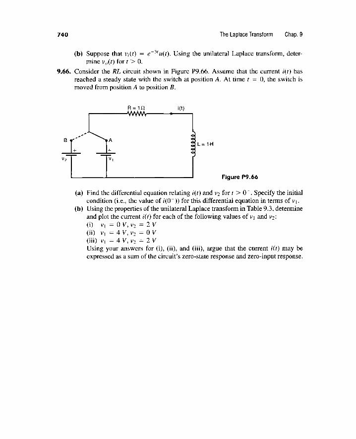
740 The Laplace Transform Chap.9
(b) Suppose that v;(t) = e- 31 u(t). Using the unilateral Laplace transform, determine v0 (t) fort > 0.
9.66. Consider the RL circuit shown in Figure P9.66. Assume that the current i(t) has reached a steady state with the switch at position A. At time t = 0, the switch is moved from position A to position B.
i(t)
L=1H
Figure P9 .66
(a) Find the differential equation relating i(t) and V2 fort > o-. Specify the initial condition (i.e., the value of i(O-)) for this differential equation in terms of v1•
(b) Using the properties of the unilateral Laplace transform in Table 9.3, determine and plot the current i(t) for each of the following values of VJ and v2: (i) v1 = 0 V, v2 = 2 V (ii) v1 = 4 V, v2 = 0 V (iii) v1 = 4 V, v2 = 2 V Using your answers for (i), (ii), and (iii), argue that the current i(t) may be expressed as a sum of the circuit's zero-state response and zero-input response.