The JPEG Image Code Format - Massey Universitymjjohnso/notes/59731/presentations/jpeg.pdf · JPEG Image Code Format 140.429 ... Conversion to the Frequency Domain 10 ... Silicon Graphics

JPEG Image Code Format 140.429

Neeraj Kashyap Page 1 Jitesh Modi

INDEX

Introduction 2 What Is an Image, Anyway? 3 Transparency 3 File Formats 4 Bandwidth and Transmission 5 An Introduction to Image Compression 5 Information Theory 7 Compression Summary 7 The JPEG Algorithm 7 Phase One: Divide the Image 8 Phase Two: Conversion to the Frequency Domain 10 Phase Three: Quantization 11 Phase Four: Entropy Coding 13 Other JPEG Information 15 Color Images 15 Decompression 16 Sources of Loss in an Image 16 Progressive JPEG Images 18 Running Time 18 Variants of the JPEG Algorithm 19 JFIF (JPEG file interchange format) 19 JBIG Compression 19 JTIP (JPEG Tiled Image Pyramid) 19 JPEG 2000 19 Conclusion 20 References 21



Introduction Multimedia images have become a vital and ubiquitous component of everyday life. The amount of information encoded in an image is quite large. Even with the advances in bandwidth and storage capabilities, if images were not compressed many applications would be too costly. The following research project attempts to answer the following questions: What are the basic principles of image compression? When is JPEG the best image compression algorithm? How does JPEG work? What are the alternatives to JPEG? Do they have any advantages or disadvantages? Finally, what is JPEG2000?

As applications developed that needed high quality imaging, compression techniques were developed to satisfy the needs of the application. Development of these compression techniques took time and the various methods were not compatible with one another. While the number of applications increased dramatically, so did the need for an image compression format that was versatile enough to compress for all of the applications. Also, due to the nature of the human eye, certain aspects of images can be taken into account to achieve an even higher level of compression. These same aspects also allow images to be compressed in ways that adapt to their transmission.

One of the most widely used applications for digital imaging is distribution on the Internet. With its growing popularity, there is more need than ever to have a way to send large amounts of image data over small bandwidth. The JPEG compression is especially useful for this task. JPEG compression is able to take advantage of the eyes lack of sensitivity to high frequency changes in the intensity of an image. Furthermore, it can compress the high frequency changes in the color information even further with close to no visible difference to the human eye, while taking up much less space. An optional extension to the JPEG standard allows for JPEG images to be encoded in a way such that as the image is transmitted over a slow connection, the image can be displayed in increasing detail. This allows the user to view several passes over the image as the image is downloaded with the image gaining detail with each pass.

Throughout the course of this document, it is hoped that it will provide a clear understanding of how JPEG compression works. Each step of the JPEG compression process will be explained and implemented.



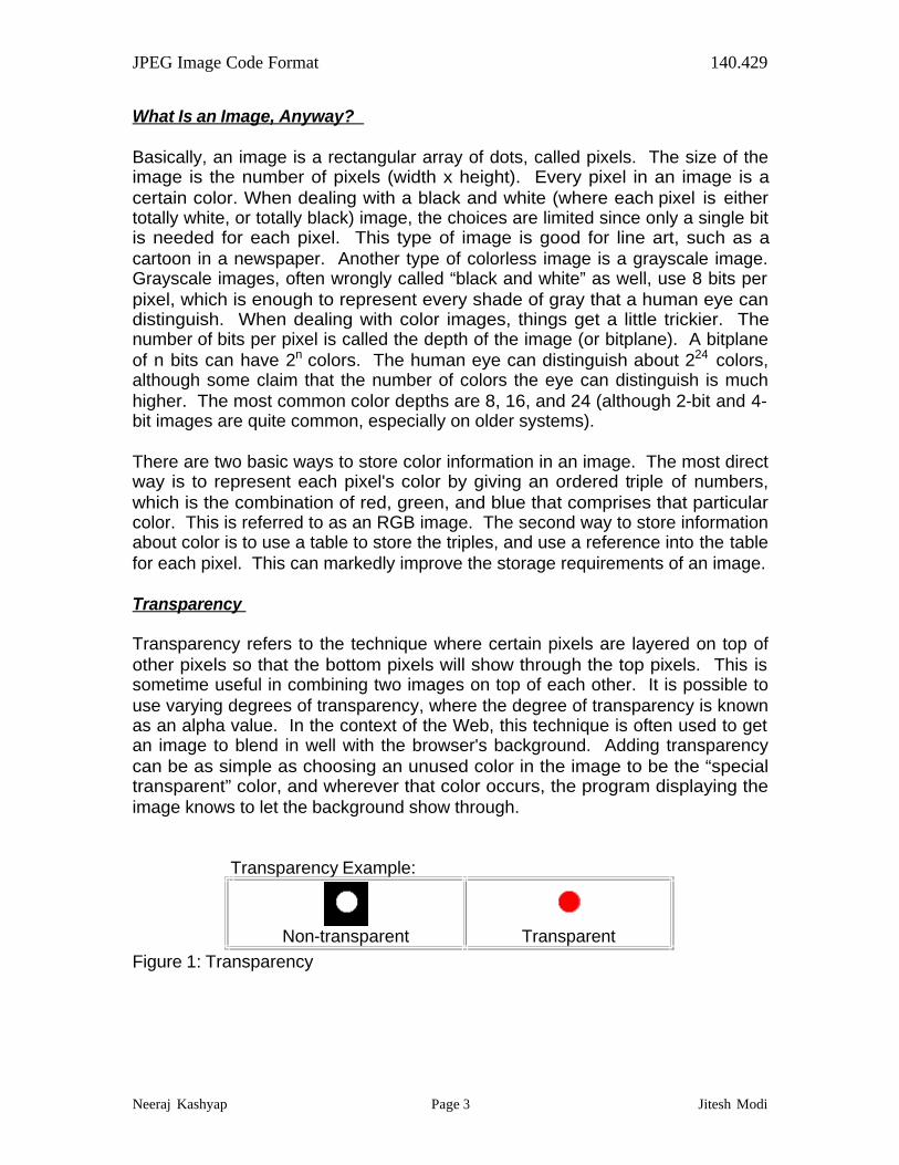
What Is an Image, Anyway? Basically, an image is a rectangular array of dots, called pixels. The size of the image is the number of pixels (width x height). Every pixel in an image is a certain color. When dealing with a black and white (where each pixel is either totally white, or totally black) image, the choices are limited since only a single bit is needed for each pixel. This type of image is good for line art, such as a cartoon in a newspaper. Another type of colorless image is a grayscale image. Grayscale images, often wrongly called “black and white” as well, use 8 bits per pixel, which is enough to represent every shade of gray that a human eye can distinguish. When dealing with color images, things get a little trickier. The number of bits per pixel is called the depth of the image (or bitplane). A bitplane of n bits can have 2n colors. The human eye can distinguish about 224 colors, although some claim that the number of colors the eye can distinguish is much higher. The most common color depths are 8, 16, and 24 (although 2-bit and 4-bit images are quite common, especially on older systems). There are two basic ways to store color information in an image. The most direct way is to represent each pixel's color by giving an ordered triple of numbers, which is the combination of red, green, and blue that comprises that particular color. This is referred to as an RGB image. The second way to store information about color is to use a table to store the triples, and use a reference into the table for each pixel. This can markedly improve the storage requirements of an image. Transparency Transparency refers to the technique where certain pixels are layered on top of other pixels so that the bottom pixels will show through the top pixels. This is sometime useful in combining two images on top of each other. It is possible to use varying degrees of transparency, where the degree of transparency is known as an alpha value. In the context of the Web, this technique is often used to get an image to blend in well with the browser's background. Adding transparency can be as simple as choosing an unused color in the image to be the “special transparent” color, and wherever that color occurs, the program displaying the image knows to let the background show through.

Transparency Example:

Non-transparent

Transparent

Figure 1: Transparency



File Formats There are a large number of file formats (hundreds) used to represent an image, some more common then others. Among the most popular are: GIF (Graphics Interchange Format) The most common image format on the Web. Stores 1 to 8-bit color or grayscale images. TIFF (Tagged Image File Format) The standard image format found in most paint, imaging, and desktop publishing programs. Supports 1- to 24- bit images and several different compression schemes. SGI Image Silicon Graphics' native image file format. Stores data in 24-bit RGB color. Sun Raster Sun's native image file format; produced by many programs that run on Sun workstations. PICT Macintosh's native image file format; produced by many programs that run on Macs. Stores up to 24-bit color. BMP (Microsoft Windows Bitmap) Main format supported by Microsoft Windows. Stores 1-, 4-, 8-, and 24-bit images. XBM (X Bitmap) A format for monochrome (1-bit) images common in the X Windows system. JPEG File Interchange Format Developed by the Joint Photographic Experts Group, sometimes simply called the JPEG file format. It can store up to 24-bits of color. Some Web browsers can display JPEG images inline (in particular, Netscape can), but this feature is not a part of the HTML standard.



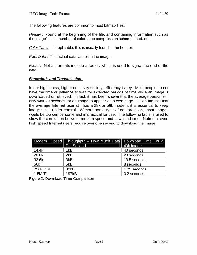
The following features are common to most bitmap files: Header : Found at the beginning of the file, and containing information such as the image's size, number of colors, the compression scheme used, etc. Color Table : If applicable, this is usually found in the header. Pixel Data : The actual data values in the image. Footer : Not all formats include a footer, which is used to signal the end of the data. Bandwidth and Transmission In our high stress, high productivity society, efficiency is key. Most people do not have the time or patience to wait for extended periods of time while an image is downloaded or retrieved. In fact, it has been shown that the average person will only wait 20 seconds for an image to appear on a web page. Given the fact that the average Internet user still has a 28k or 56k modem, it is essential to keep image sizes under control. Without some type of compression, most images would be too cumbersome and impractical for use. The following table is used to show the correlation between modem speed and download time. Note that even high speed Internet users require over one second to download the image.

Modem Speed

Throughput – How Much Data Per Second

Download Time For a 40k Image

14.4k 1kB 40 seconds 28.8k 2kB 20 seconds 33.6k 3kB 13.5 seconds 56k 5kB 8 seconds 256k DSL 32kB 1.25 seconds 1.5M T1 197kB 0.2 seconds

Figure 2: Download Time Comparison



An Introduction to Image Compression Image compression is the process of reducing the amount of data required to represent a digital image. Removing all redundant or unnecessary information does this. An uncompressed image requires an enormous amount of data to represent it. As an example, a standard 8.5" by 11" sheet of paper scanned at 100 dpi and restricted to black and white requires more then 100k bytes to represent. Another example is the 276-pixel by 110-pixel banner that appears at the top of Google.com. Uncompressed, it requires 728k of space. Image compression is thus essential for the efficient storage, retrieval and transmission of images. In general, there are two main categories of compression. Lossless compression involves the preservation of the image as is (with no information and thus no detail lost). Lossy compression on the other hand, allows less then perfect reproductions of the original image. The advantage being that, with a lossy algorithm, one can achieve higher levels of compression because less information is needed. Various amounts of data may be used to represent the same amount of information. Some representations may be less efficient than others, depending on the amount of redundancy eliminated from the data. When talking about images there are three main sources of redundant information: Coding Redundancy - This refers to the binary code used to represent gray values. Interpixel Redundancy - This refers to the correlation between adjacent pixels in an image. Psychovisual Redundancy - This refers to the unequal sensitivity of the human eye to different visual information. In comparing how much compression one algorithm achieves verses another, many people talk about a compression ratio. A higher compression ratio indicates that one algorithm removes more redundancy then another (and thus is more efficient). If n1 and n2 are the number of bits in two datasets that represent the same image, the relative redundancy of the first dataset is defined as: Rd=1/CR, where CR (the compression ratio) =n1/n2 The benefits of compression are immense. If an image is compressed at a ratio of 100:1, it may be transmitted in one hundredth of the time, or transmitted at the same speed through a channel of one-hundredth the bandwidth (ignoring the compression/decompression overhead). Since images have become so commonplace and so essential to the function of computers, it is hard to see how we would function without them.



Compression Summary Image compression is achieved by removing (or reducing) redundant information. In order to effectively do this, patterns in the data must be identified and utilized. The theoretical basis for this is founded in Information theory, which assigns probabilities to the likelihood of the occurrence of each symbol in the input. Symbols with a high probability of occurring are represented with shorter bit strings (or code words). Conversely, symbols with a low probability of occurring are represented with longer code words. In this way, the average length of code words is decreased, and redundancy is reduced. How efficient an algorithm can be, depends in part on how the probability of the symbols is distributed, with maximum efficiency occurring when the distribution is equal over all input symbols.



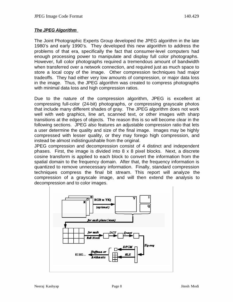
The JPEG Algorithm The Joint Photographic Experts Group developed the JPEG algorithm in the late 1980’s and early 1990’s. They developed this new algorithm to address the problems of that era, specifically the fact that consumer-level computers had enough processing power to manipulate and display full color photographs. However, full color photographs required a tremendous amount of bandwidth when transferred over a network connection, and required just as much space to store a local copy of the image. Other compression techniques had major tradeoffs. They had either very low amounts of compression, or major data loss in the image. Thus, the JPEG algorithm was created to compress photographs with minimal data loss and high compression ratios. Due to the nature of the compression algorithm, JPEG is excellent at compressing full-color (24-bit) photographs, or compressing grayscale photos that include many different shades of gray. The JPEG algorithm does not work well with web graphics, line art, scanned text, or other images with sharp transitions at the edges of objects. The reason this is so will become clear in the following sections. JPEG also features an adjustable compression ratio that lets a user determine the quality and size of the final image. Images may be highly compressed with lesser quality, or they may forego high compression, and instead be almost indistinguishable from the original. JPEG compression and decompression consist of 4 distinct and independent phases. First, the image is divided into 8 x 8 pixel blocks. Next, a discrete cosine transform is applied to each block to convert the information from the spatial domain to the frequency domain. After that, the frequency information is quantized to remove unnecessary information. Finally, standard compression techniques compress the final bit stream. This report will analyze the compression of a grayscale image, and will then extend the analysis to decompression and to color images.



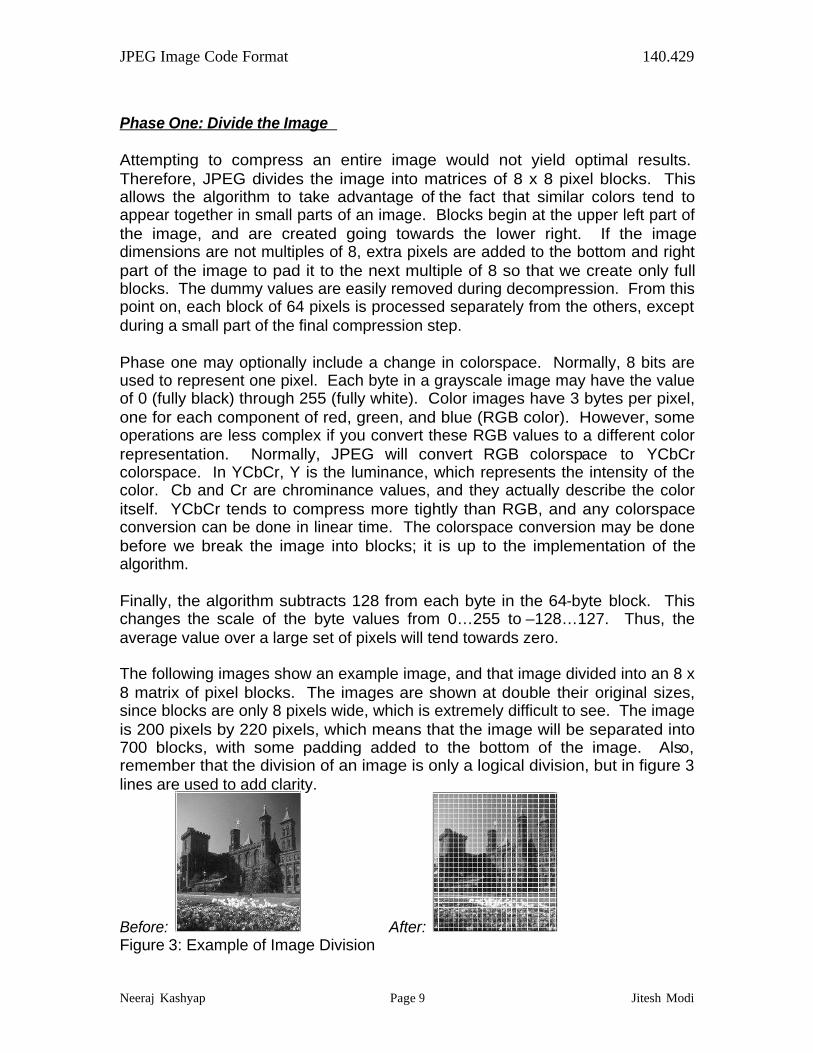
Phase One: Divide the Image Attempting to compress an entire image would not yield optimal results. Therefore, JPEG divides the image into matrices of 8 x 8 pixel blocks. This allows the algorithm to take advantage of the fact that similar colors tend to appear together in small parts of an image. Blocks begin at the upper left part of the image, and are created going towards the lower right. If the image dimensions are not multiples of 8, extra pixels are added to the bottom and right part of the image to pad it to the next multiple of 8 so that we create only full blocks. The dummy values are easily removed during decompression. From this point on, each block of 64 pixels is processed separately from the others, except during a small part of the final compression step. Phase one may optionally include a change in colorspace. Normally, 8 bits are used to represent one pixel. Each byte in a grayscale image may have the value of 0 (fully black) through 255 (fully white). Color images have 3 bytes per pixel, one for each component of red, green, and blue (RGB color). However, some operations are less complex if you convert these RGB values to a different color representation. Normally, JPEG will convert RGB colorspace to YCbCr colorspace. In YCbCr, Y is the luminance, which represents the intensity of the color. Cb and Cr are chrominance values, and they actually describe the color itself. YCbCr tends to compress more tightly than RGB, and any colorspace conversion can be done in linear time. The colorspace conversion may be done before we break the image into blocks; it is up to the implementation of the algorithm. Finally, the algorithm subtracts 128 from each byte in the 64-byte block. This changes the scale of the byte values from 0…255 to –128…127. Thus, the average value over a large set of pixels will tend towards zero. The following images show an example image, and that image divided into an 8 x 8 matrix of pixel blocks. The images are shown at double their original sizes, since blocks are only 8 pixels wide, which is extremely difficult to see. The image is 200 pixels by 220 pixels, which means that the image will be separated into 700 blocks, with some padding added to the bottom of the image. Also, remember that the division of an image is only a logical division, but in figure 3 lines are used to add clarity.

Before: After: Figure 3: Example of Image Division



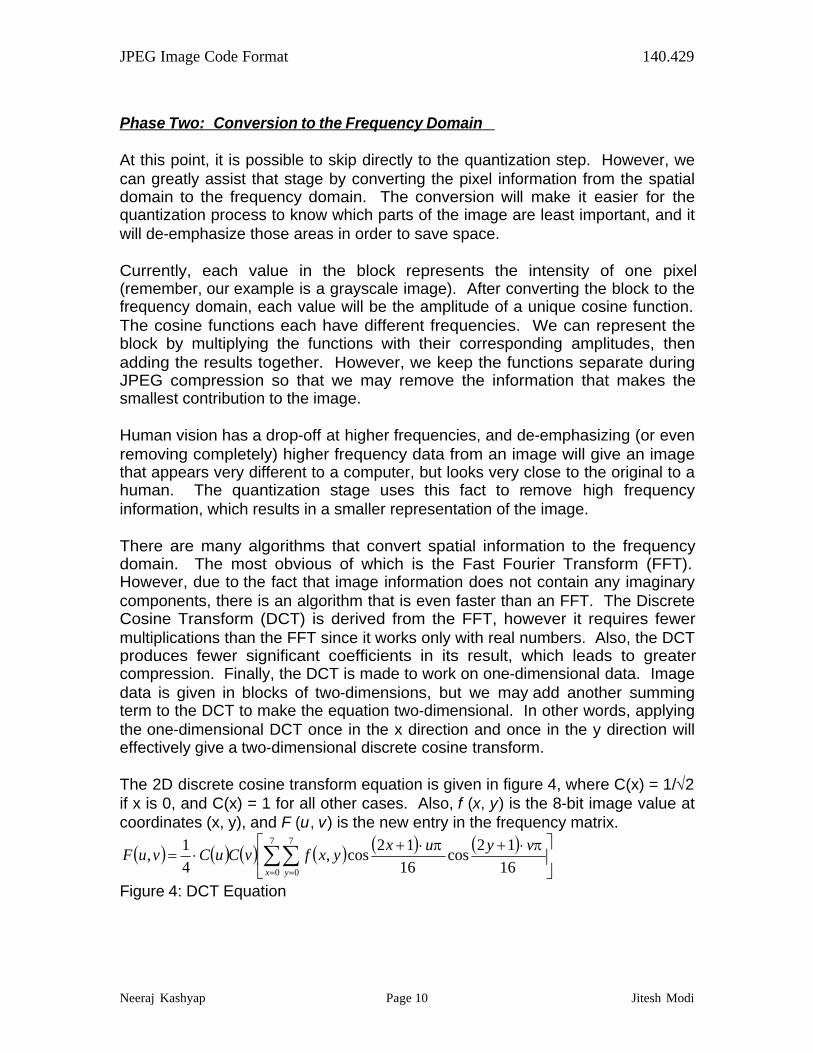
Phase Two: Conversion to the Frequency Domain At this point, it is possible to skip directly to the quantization step. However, we can greatly assist that stage by converting the pixel information from the spatial domain to the frequency domain. The conversion will make it easier for the quantization process to know which parts of the image are least important, and it will de-emphasize those areas in order to save space. Currently, each value in the block represents the intensity of one pixel (remember, our example is a grayscale image). After converting the block to the frequency domain, each value will be the amplitude of a unique cosine function. The cosine functions each have different frequencies. We can represent the block by multiplying the functions with their corresponding amplitudes, then adding the results together. However, we keep the functions separate during JPEG compression so that we may remove the information that makes the smallest contribution to the image. Human vision has a drop-off at higher frequencies, and de-emphasizing (or even removing completely) higher frequency data from an image will give an image that appears very different to a computer, but looks very close to the original to a human. The quantization stage uses this fact to remove high frequency information, which results in a smaller representation of the image. There are many algorithms that convert spatial information to the frequency domain. The most obvious of which is the Fast Fourier Transform (FFT). However, due to the fact that image information does not contain any imaginary components, there is an algorithm that is even faster than an FFT. The Discrete Cosine Transform (DCT) is derived from the FFT, however it requires fewer multiplications than the FFT since it works only with real numbers. Also, the DCT produces fewer significant coefficients in its result, which leads to greater compression. Finally, the DCT is made to work on one-dimensional data. Image data is given in blocks of two-dimensions, but we may add another summing term to the DCT to make the equation two-dimensional. In other words, applying the one-dimensional DCT once in the x direction and once in the y direction will effectively give a two-dimensional discrete cosine transform. The 2D discrete cosine transform equation is given in figure 4, where C(x) = 1/Ö2 if x is 0, and C(x) = 1 for all other cases. Also, f (x, y) is the 8-bit image value at coordinates (x, y), and F (u, v) is the new entry in the frequency matrix.

( ) ( ) ( ) ( ) ( ) ( )úû

ùêë

é ×+×+×= åå

= =

7

0

7

0 16

12cos

16

12cos,

4

1,

x y

vyuxyxfvCuCvuF

pp

Figure 4: DCT Equation



We begin examining this formula by realizing that only constants come before the brackets. Next, we realize that only 16 different cosine terms will be needed for each different pair of (u, v) values, so we may compute these ahead of time and then multiply the correct pair of cosine terms to the spatial-domain value for that pixel. There will be 64 additions in the two summations, one per pixel. Finally, we multiply the sum by the 3 constants to get the final value in the frequency matrix. This continues for all (u, v) pairs in the frequency matrix. Since u and v may be any value from 0…7, the frequency domain matrix is just as large as the spatial domain matrix. The frequency domain matrix contains values from -1024…1023. The upper-left entry, also known as the DC value, is the average of the entire block, and is the lowest frequency cosine coefficient. As you move right the coefficients represent cosine functions in the vertical direction that increase in frequency. Likewise, as you move down, the coefficients belong to increasing frequency cosine functions in the horizontal direction. The highest frequency values occur at the lower-right part of the matrix. The higher frequency values also have a natural tendency to be significantly smaller than the low frequency coefficients since they contribute much less to the image. Typically the entire lower-right half of the matrix is factored out after quantization. This essentially removes half of the data per block, which is one reason why JPEG is so efficient at compression. Computing the DCT is the most time-consuming part of JPEG compression. Thus, it determines the worst-case running time of the algorithm. The running time of the algorithm is discussed in detail later. However, there are many different implementations of the discrete cosine transform. Finding the most efficient one for the programmer’s situation is key. There are implementations that can replace all multiplications with shift instructions and additions. Doing so can give dramatic speedups, however it often approximates values, and thus leads to a lower quality output image. There are also debates on how accurately certain DCT algorithms compute the cosine coefficients, and whether or not the resulting values have adequate precision for their situations. So any programmer should use caution when choosing an algorithm for computing a DCT, and should be aware of every trade-off that the algorithm has.



Phase Three: Quantization Having the data in the frequency domain allows the algorithm to discard the least significant parts of the image. The JPEG algorithm does this by dividing each cosine coefficient in the data matrix by some predetermined constant, and then rounding up or down to the closest integer value. The constant values that are used in the division may be arbitrary, although research has determined some very good typical values. However, since the algorithm may use any values it wishes, and since this is the step that introduces the most loss in the image, it is a good place to allow users to specify their desires for quality versus size. Obviously, dividing by a high constant value can introduce more error in the rounding process, but high constant values have another effect. As the constant gets larger the result of the division approaches zero. This is especially true for the high frequency coefficients, since they tend to be the smallest values in the matrix. Thus, many of the frequency values become zero. Phase four takes advantage of this fact to further compress the data. The algorithm uses the specified final image quality level to determine the constant values that are used to divide the frequencies. A constant of 1 signifies no loss. On the other hand, a constant of 255 is the maximum amount of loss for that coefficient. The constants are calculated according to the user’s wishes and the heuristic values that are known to result in the best quality final images. The constants are then entered into another 8 x 8 matrix, called the quantization matrix. Each entry in the quantization matrix corresponds to exactly one entry in the frequency matrix. Simply coordinates determine correspondence; the entry at (3, 5) in the quantization matrix corresponds to entry (3, 5) in the frequency matrix. A typical quantization matrix will be symmetrical about the diagonal, and will have lower values in the upper left and higher values in the lower right. Since any arbitrary values could be used during quantization, the entire quantization matrix is stored in the final JPEG file so that the decompression routine will know the values that were used to divide each coefficient.



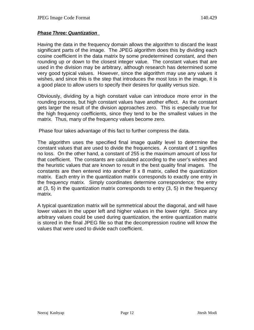
Figure 5 shows an example of a quantization matrix.

Figure 5: Sample Quantization Matrix

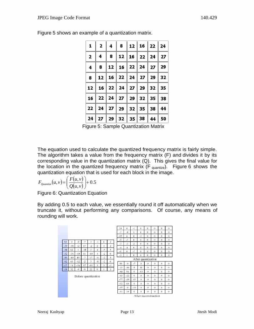
The equation used to calculate the quantized frequency matrix is fairly simple. The algorithm takes a value from the frequency matrix (F) and divides it by its corresponding value in the quantization matrix (Q). This gives the final value for the location in the quantized frequency matrix (F quantize). Figure 6 shows the quantization equation that is used for each block in the image.

( ) ( )( )

5.0,

,, +÷÷

ø

öççè

æ=

vuQ

vuFvuFQuantize

Figure 6: Quantization Equation By adding 0.5 to each value, we essentially round it off automatically when we truncate it, without performing any comparisons. Of course, any means of rounding will work.



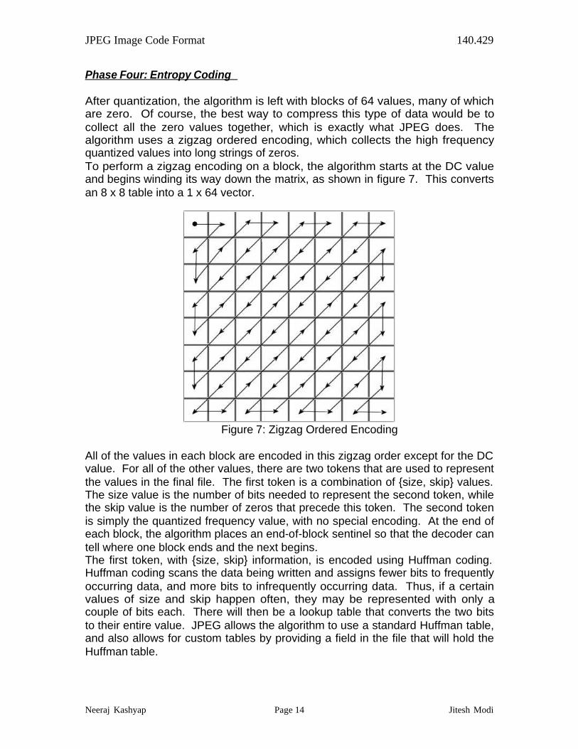
Phase Four: Entropy Coding After quantization, the algorithm is left with blocks of 64 values, many of which are zero. Of course, the best way to compress this type of data would be to collect all the zero values together, which is exactly what JPEG does. The algorithm uses a zigzag ordered encoding, which collects the high frequency quantized values into long strings of zeros. To perform a zigzag encoding on a block, the algorithm starts at the DC value and begins winding its way down the matrix, as shown in figure 7. This converts an 8 x 8 table into a 1 x 64 vector.

Figure 7: Zigzag Ordered Encoding

All of the values in each block are encoded in this zigzag order except for the DC value. For all of the other values, there are two tokens that are used to represent the values in the final file. The first token is a combination of {size, skip} values. The size value is the number of bits needed to represent the second token, while the skip value is the number of zeros that precede this token. The second token is simply the quantized frequency value, with no special encoding. At the end of each block, the algorithm places an end-of-block sentinel so that the decoder can tell where one block ends and the next begins. The first token, with {size, skip} information, is encoded using Huffman coding. Huffman coding scans the data being written and assigns fewer bits to frequently occurring data, and more bits to infrequently occurring data. Thus, if a certain values of size and skip happen often, they may be represented with only a couple of bits each. There will then be a lookup table that converts the two bits to their entire value. JPEG allows the algorithm to use a standard Huffman table, and also allows for custom tables by providing a field in the file that will hold the Huffman table.



DC values use delta encoding, which means that each DC value is compared to the previous value, in zigzag order. Note that comparing DC values is done on a block-by-block basis, and does not consider any other data within a block. This is the only instance where blocks are not treated independently from each other. The difference between the current DC value and the previous value is all that is included in the file. When storing the DC values, JPEG includes a size field and then the actual DC delta value. So if the difference between two adjacent DC values is –4, JPEG will store the size 3, since -4 requires 3 bits. Then, the actual binary value 100 is stored. The size field for DC values is included in the Huffman coding for the other size values, so that JPEG can achieve even higher compression of the data. Other JPEG Information There are other facts about JPEG that are not covered in the compression of a grayscale image. The following sections describe other parts of the JPEG algorithm, such as decompression, progressive JPEG encoding, and the algorithm’s running time. Color Images Color images are usually encoded in RGB colorspace, where each pixel has an 8-bit value for each of the three composite colors. Thus, a color image is three times as large as a grayscale image, and each of the components of a color image can be considered its own grayscale representation of that particular color. In fact, JPEG treats a color image as 3 separate grayscale images, and compresses each component in the same way it compresses a grayscale image. However, most color JPEG files are not three times larger than a grayscale image, since there is usually one color component that does not occur as often as the others, in which case it will be highly compressed. Also, the Huffman coding steps will have the opportunity to compress more values, since there are more possible values to compress.



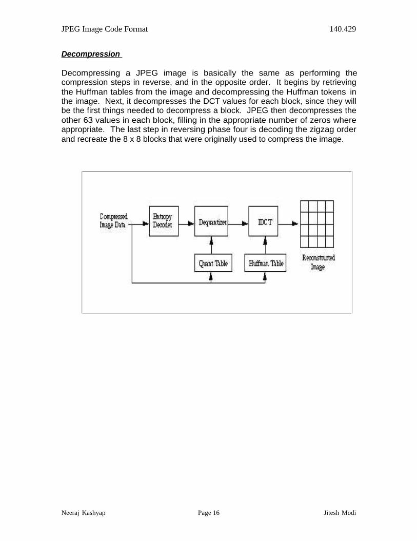
Decompression Decompressing a JPEG image is basically the same as performing the compression steps in reverse, and in the opposite order. It begins by retrieving the Huffman tables from the image and decompressing the Huffman tokens in the image. Next, it decompresses the DCT values for each block, since they will be the first things needed to decompress a block. JPEG then decompresses the other 63 values in each block, filling in the appropriate number of zeros where appropriate. The last step in reversing phase four is decoding the zigzag order and recreate the 8 x 8 blocks that were originally used to compress the image.



Sources of Loss in an Image JPEG is a lossy algorithm. Compressing an image with this algorithm will almost guarantee that the decompressed version of the image will not match the original source image. Loss of information happens in phases two and three of the algorithm. In phase two, the discrete cosine transformation introduces some error into the image, however this error is very slight. The error is due to imprecision in multiplication, rounding, and significant error is possible if the DCT implementation chosen by the programmer is designed to trade off quality for speed. Any errors introduced in this phase can affect any values in the image with equal probability. It does not limit its error to any particular section of the image. Phase three, on the other hand, is designed to eliminate data that does not contribute much to the image. In fact, most of the loss in JPEG compression occurs during this phase. Quantization divides each frequency value by a constant, and rounds the result. Therefore, higher constants cause higher amounts of loss in the frequency matrix, since the rounding error will be higher. As stated before, the algorithm is designed in this way, since the higher constants are concentrated around the highest frequencies, and human vision is not very sensitive to those frequencies. Also, the quantization matrix is adjustable, so a user may adjust the amount of error introduced into the compressed image. Obviously, as the algorithm becomes less lossy, the image size increases. Applications that allow the creation of JPEG images usually allow a user to specify some value between 1 and 100, where 100 is the least lossy. By most standards, anything over 90 or 95 does not make the picture any better to the human eye, but it does increase the file size dramatically. Alternatively, very low values will create extremely small files, but the files will have a blocky effect. In fact, some graphics artists use JPEG at very low quality settings (under 5) to create stylized effects in their photos.



Progressive JPEG Images A newer version of JPEG allows images to be encoded as progressive JPEG images. A progressive image, when downloaded, will show the major features of the image very quickly, and will then slowly become clearer as the rest of the image is received. Normally, an image is displayed at full clarity, and is shown from top to bottom as it is received and decoded. Progressive JPEG files are useful for slow connections, since a user can get a good idea what the picture will be well before it finishes downloading. Note that progressive JPEG is simply a rearrangement of data onto a more complicated order, and does not actually change any major aspects of the JPEG format. Also, a progressive JPEG file will be the same size as a standard JPEG file. Finally, displaying progressive JPEG images is more computationally intense than displaying a standard JPEG, since some extra processing is needed to make the image fade into view. There are two main ways to implement a progressive JPEG. The first, and easiest, is to simply display the DC values as they are received. The DC values, being the average value of the 8 x 8 block, are used to represent the entire block. Thus, the progressive image will appear as a blocky image while the other values are received, but since the blocks are so small, a fairly adequate representation of the image will be shown using just the DC values. The alternative method is to begin by displaying just the DC information, as detailed above. But then, as the data is received, it will begin to add some higher frequency values into the image. This makes the image appear to gain sharpness until the final image is displayed. To implement this, JPEG first encodes the image so that certain lower frequencies will be received very quickly. The lower frequency values are displayed as they are received, and as more bits of each frequency value are received they are shifted into place and the image is updated.



Variants of the JPEG Algorithm Quite a few algorithms are based on JPEG. They were created for more specific purposes than the more general JPEG algorithm. This section will discuss variations on JPEG. Also, since the output stream from the JPEG algorithm must be saved to disk, we discuss the most common JPEG file format. 1. JFIF (JPEG file interchange format) 2. JBIG Compression 3. JTIP (JPEG Tiled Image Pyramid) 4. JPEG 2000 JPEG 2000 JPEG 2000 is the “next big thing” in image compression. It is designed to overcome many of the drawbacks that JPEG had, such as the amount of loss introduced into computer-generated art and bi-level images. Unfortunately, the final standard is not complete, but some general information about JPEG 2000 is available, and it is presented here. This algorithm relies on wavelets to convert the image from the spatial domain to the frequency domain. Wavelets are much better at representing local features in a function, and thus create less loss in the image. In fact, JPEG 2000 has a loss less compression mode that is able to compress an image much better than JPEG’s loss less mode. Another benefit of using wavelets is that a wavelet can examine the image at multiple resolutions, and determine exactly how to process the image. Another benefit of JPEG 2000 is that it considers an entire image at once, instead of splitting the image into blocks. Also, JPEG 2000 scales very well, and can provide good quality images at low bit rates. This will be important, since devices like cellular phones are now capable of displaying images. Finally, JPEG 2000 is much better at compressing an image while maintaining high quality. Given a source image, if one compares a JPEG image with a JPEG 2000 image (assuming both are compressed to the same final size), the JPEG 2000 image will be much clearer, and will never have the blocky look that JPEG can sometimes introduce into an image.



Conclusion The JPEG algorithm was created to compress photographic images, and it does this very well, with high compression ratios. It also allows a user to choose between high quality output images, or very small output images. The algorithm compresses images in 4 distinct phases, and does so in ( )( )nn log2O time, or

better. It also inspired many other algorithms that compress images and video, and do so in a fashion very similar to JPEG. Most of the variants of JPEG take the basic concepts of the JPEG algorithm and apply them to more specific problems. Due to the immense number of JPEG images that exist, this algorithm will probably be in use for at least 10 more years. This is despite the fact that better algorithms for compressing images exist, and even better ones than those will be ready in the near future.



References 1. http://www.jpeg.org 2. www.faqs.org/faqs/ jpeg-faq/part1 3. http://www.faqs.org/faqs/compression -faq/ 4. http://www.fu zzymonkey.org/projects/ece472_jpeg_encoding/

http://www.jpeg.org/

http://www.faqs.org/faqs/jpeg-faq/part1




http://www.faqs.org/faqs/compression-faq/



Documents

The JPEG Image Code Format - Massey Universitymjjohnso/notes/59731/presentations/jpeg.pdf · JPEG Image Code Format 140.429 ... Conversion to the Frequency Domain 10 ... Silicon Graphics