Embed Size (px)
Citation preview

The Join Calculus:a Language for Distributed Mobile Programming
Cedric Fournet1 and Georges Gonthier2?
1 Microsoft Research2 INRIA Rocquencourt
Abstract In these notes, we give an overview of the join calculus, itssemantics, and its equational theory. The join calculus is a language thatmodels distributed and mobile programming. It is characterized by anexplicit notion of locality, a strict adherence to local synchronization, anda direct embedding of the ML programming language. The join calculus isused as the basis for several distributed languages and implementations,such as JoCaml and functional nets.Local synchronization means that messages always travel to a set des-tination, and can interact only after they reach that destination; thisis required for an efficient implementation. Specifically, the join calcu-lus uses ML’s function bindings and pattern-matching on messages toprogram these synchronizations in a declarative manner.Formally, the language owes much to concurrency theory, which providesa strong basis for stating and proving the properties of asynchronousprograms. Because of several remarkable identities, the theory of processequivalences admits simplifications when applied to the join calculus.We prove several of these identities, and argue that equivalences for thejoin calculus can be rationally organized into a five-tiered hierarchy, withsome trade-off between expressiveness and proof techniques.We describe the mobility extensions of the core calculus, which allow theprogramming of agent creation and migration. We briefly present howthe calculus has been extended to model distributed failures on the onehand, and cryptographic protocols on the other.
? This work is partly supported by the RNRT project MARVEL 98S0347
Applied Semantics Summer School (Caminha, 9–15 September 2000)Draft 7/01, pp. 1–66,

Contents
The Join Calculus: a Language for Distributed Mobile Programming . . . . . . . . . . 1Cedric Fournet, Georges Gonthier
1 The core join calculus . . . . . . . . . . . . . . . . . . . . . . . . . . . . . . . . . . . . . . . . . . . . . . . . 51.1 Concurrent functional programming . . . . . . . . . . . . . . . . . . . . . . . . . . . . . . . 51.2 Synchronization by pattern-matching . . . . . . . . . . . . . . . . . . . . . . . . . . . . . . 71.3 The asynchronous core . . . . . . . . . . . . . . . . . . . . . . . . . . . . . . . . . . . . . . . . . . 121.4 Operational semantics . . . . . . . . . . . . . . . . . . . . . . . . . . . . . . . . . . . . . . . . . . . 141.5 The reflexive chemical abstract machine . . . . . . . . . . . . . . . . . . . . . . . . . . . 16
2 Basic equivalences . . . . . . . . . . . . . . . . . . . . . . . . . . . . . . . . . . . . . . . . . . . . . . . . . . . 202.1 May testing equivalence . . . . . . . . . . . . . . . . . . . . . . . . . . . . . . . . . . . . . . . . . 212.2 Trace observation . . . . . . . . . . . . . . . . . . . . . . . . . . . . . . . . . . . . . . . . . . . . . . . 242.3 Simulation and coinduction . . . . . . . . . . . . . . . . . . . . . . . . . . . . . . . . . . . . . . 262.4 Bisimilarity equivalence . . . . . . . . . . . . . . . . . . . . . . . . . . . . . . . . . . . . . . . . . . 292.5 Bisimulation proof techniques . . . . . . . . . . . . . . . . . . . . . . . . . . . . . . . . . . . . 30
3 A hierarchy of equivalences . . . . . . . . . . . . . . . . . . . . . . . . . . . . . . . . . . . . . . . . . . . 333.1 Too many equivalences? . . . . . . . . . . . . . . . . . . . . . . . . . . . . . . . . . . . . . . . . . 333.2 Fair testing . . . . . . . . . . . . . . . . . . . . . . . . . . . . . . . . . . . . . . . . . . . . . . . . . . . . 363.3 Coupled Simulations . . . . . . . . . . . . . . . . . . . . . . . . . . . . . . . . . . . . . . . . . . . . 373.4 Two notions of congruence . . . . . . . . . . . . . . . . . . . . . . . . . . . . . . . . . . . . . . . 413.5 Summary: a hierarchy of equivalences . . . . . . . . . . . . . . . . . . . . . . . . . . . . . 44
4 Labeled semantics . . . . . . . . . . . . . . . . . . . . . . . . . . . . . . . . . . . . . . . . . . . . . . . . . . . 454.1 Open syntax and chemistry . . . . . . . . . . . . . . . . . . . . . . . . . . . . . . . . . . . . . . 454.2 Observational equivalences on open terms . . . . . . . . . . . . . . . . . . . . . . . . . . 484.3 Labeled bisimulation . . . . . . . . . . . . . . . . . . . . . . . . . . . . . . . . . . . . . . . . . . . . 494.4 Asynchronous bisimulation . . . . . . . . . . . . . . . . . . . . . . . . . . . . . . . . . . . . . . . 504.5 The discriminating power of name comparison . . . . . . . . . . . . . . . . . . . . . . 52
5 Distribution and mobility . . . . . . . . . . . . . . . . . . . . . . . . . . . . . . . . . . . . . . . . . . . . . 545.1 Distributed mobile programming. . . . . . . . . . . . . . . . . . . . . . . . . . . . . . . . . . 545.2 Computing with locations . . . . . . . . . . . . . . . . . . . . . . . . . . . . . . . . . . . . . . . . 575.3 Attaching some meaning to locations . . . . . . . . . . . . . . . . . . . . . . . . . . . . . . 62

The Join Calculus: a Language for Distributed Mobile Programming 3
Introduction
Wide-area distributed systems have become an important part of modern pro-gramming, yet most distributed programs are still written using traditional lan-guages, designed for sequential architectures. Distribution issues are typicallyrelegated to libraries and informal design patterns, with little support in thelanguage for asynchrony and concurrency. Conversely, distributed constructs areinfluenced by the local programming model, with for instance a natural bias to-wards RPCs or RMIs rather than asynchronous message passing.
Needless to say, distributed programs are usually hard to write, much harderto understand and to relate to their specifications, and almost impossible todebug. This is due to essential difficulties, such as asynchrony or partial failures.Nonetheless, it should be possible to provide some high-level language supportto address these issues.
The join calculus is an attempt to provide language support for asynchronous,distributed, and mobile programming. While it is clearly not the only approach,it has a simple and well-defined model, which has been used as the basis forseveral language implementations and also as a specification language for study-ing the properties of such programs. These notes give an overview of the model,with an emphasis on its operational semantics and its equational theory.
JoCaml [27] is the latest implementation of the join calculus; it is a dis-tributed extension of Objective Caml [29], a typed high-level programming lan-guage with a mix of functional, object-oriented, and imperative features. OCamlalready provides native-code and bytecode compilers, which is convenient formobile code. The JoCaml language extends OCaml, in the sense that OCamlprograms and libraries are just a special kind of JoCaml programs and libraries.JoCaml also implements strong mobility and provides support for distributedexecution, including a dynamic linker and a garbage collector. The languagedocumentation includes extensive tutorials; they can be seen as a concrete coun-terpart for the material presented in these notes (Sections 1 and 5) with largerprogramming examples.
In these notes, we present a core calculus, rather than a full-fledged lan-guage. This minimalist approach enables us to focus on the essential featuresof the language, and to develop a simple theory: the calculus provides a precisedescription of how the distributed implementation should behave and, at thesame time, it yields a formal model that is very close to the actual programminglanguage. Thus, one can directly study the correctness of distributed programs,considering them as executable specifications. Ideally, the model should providestrong guiding principles for language design and, conversely, the model shouldreflect the implementation constraints.
The join calculus started out as an attempt to take the models and methodsdeveloped by concurrency theory, and to adapt and apply them to the program-ming of systems distributed over a wide area network. The plan was to startfrom Milner’s pi calculus [31,30,41], extend it with constructs for locality andmobility, and bring to bear the considerable body of work on process calculiand their equivalences on the problem of programming mobile agents. During
4 Applied Semantics Summer School, Draft 7/01
the course of this work, the implementation constraints of asynchronous systemssuggested changing the pi calculus’s CCS-based communication model. The ideawas that the model had to stick to what all basic protocol suites do, and decoupletransmission from synchronization, so that synchronization issues can always beresolved locally.
To us, the natural primitives for doing this in a higher-order setting weremessage passing, function call, and pattern-matching, and these suggested astrong link with the programming language ML. This connection allowed us toreuse a significant portion of the ML programming technology—notably the MLtype system—for the “programming” part of our project. Thus the join calculuswas born out of the synergy between asynchronous process calculi and ML.
Many of the ideas that we adapted from either source took new meaningin the location-sensitive, asynchronous framework of the join calculus. The con-nection with ML illuminates the interaction between functional and imperativefeatures, down to their implications for typing. The highly abstract chemical ab-stract machine of Berry and Boudol [7] yields a much more operational instancefor the join calculus. The intricate lattice of equivalences for synchronous andasynchronous calculi [19] simplifies remarkably in the pure asynchronous settingof the join calculus, to the point that we can reasonably concentrate on a singlefive-tiered hierarchy of equivalences, where each tier can be clearly argued for.These lecture notes contains a summary of these results, as well as much of therationale that joins them into a coherent whole.
These notes are organized as follows. In Section 1, we gradually introduce thejoin calculus as a concurrent extension of ML, describe common synchronizationpatterns, and give its chemical semantics. In Section 2, we define and motivateour main notions of observational equivalences, and illustrate the main prooftechniques for establishing equivalences between processes. In Section 3, we refineour framework for reasoning about processes. We introduce intermediate notionsof equivalence that account for fairness and gradual commitment, and organizeall our equivalences in a hierarchy, according to their discriminating power. InSection 4, we supplement this framework with labeled semantics, and discusstheir relation. In Section 5, we finally refine the programming model to accountfor locality information and agent migration.

The Join Calculus: a Language for Distributed Mobile Programming 5
1 The core join calculus
Although the join calculus was designed as a process calculus for distributedand mobile computation, it turned out to be a close match to ML-style (impure)functional programming. In these notes we will use this connection to motivateand explain the computational core of the calculus.
First we will introduce the primitives of the join calculus by showing howthey mesh in a typical ‘mini-ML’ lambda-like calculus. At a more concrete level,there is a similar introduction to the JoCaml language as an extension of theOCaml programming language [27].
We will then show how a variety of synchronization primitives can be easilyencoded in the join calculus and argue that the general join calculus itself canbe encoded by its “asynchronous” fragment, i.e., that function calls are just aform of message-passing. This allows us to limit the formal semantics of the joincalculus to its asynchronous core.
We conclude the section by exposing the computational model that underliesthe formal semantics of the join calculus. This simple model guarantees thatdistributed computation can be faithfully represented in the join calculus.
1.1 Concurrent functional programming
Our starting point is a small ML-like syntax for the call-by-value polyadic lambdacalculus:
E,F ::= expressionsx, y, f variable
|| f(E) function call|| let x = E in F local value definition|| let f(x) = E in F local recursive function definition
The notation x stands for a possibly empty comma-separated tuple x1, x2, . . . , xnof variables; similarly E is a tuple of expressions. We casually assume that theusual Hindley-Milner type system ensures that functions are always called withthe proper number of arguments.
We depart from the lambda calculus by taking the ML-style function defi-nition as primitive, rather than λ-expressions, which can be trivially recoveredas λx.E def= let f(x) = E in f . This choice is consistent with the usual MLprogramming practice, and will allow us to integrate smoothly primitives withside effects, such as the join calculus primitives, because the let provides a syn-tactic “place” for the state of the function. An immediate benefit, however, isthat values in this calculus consist only of names: (globally) free variables, orlet-defined function names. This allows us to omit altogether curried functioncalls from our syntax, since the function variable in a call can only be replacedby a function name in a call-by-value computation.
We are going to present the join calculus as an extension of this functionalcalculus with concurrency. The most straightforward way of doing this would

6 Applied Semantics Summer School, Draft 7/01
be to add a new run E primitive that returns immediately after starting aconcurrent evaluation of E. However, we want to get a model in which we canreason about concurrent behavior, not just a programming language design. Inorder to develop an operational semantics, we also need a syntax that describesthe situation after run E returns, and the evaluation of E and the evaluationof the expression F that contained the run E proceed concurrently. It wouldbe quite awkward to use run for this, since it would force us to treat E and Fasymmetrically.
It is much more natural to denote the concurrent computation of E and F byE | F , using a parallel composition operator ‘|’. However, we must immediatelyrealize the E | F cannot be an “expression”, since an expression denotes acomputation that returns a result, and there is no natural way of defining aunique “result” for E | F . Therefore we need to extend our calculus with asecond sort for processes, i.e., computations that aren’t expected to produce aresult (and hence, don’t terminate). In fact, the operands E and F of E | Fshould also be processes, rather than expressions, since they aren’t expected toreturn a result either. Thus, ‘|’ will simply be an operation on processes.
We will use the letters P,Q,R for processes. We still need the run P primitiveto launch a process from an expression; conversely, we allow let constructs inprocesses, so that processes can evaluate expressions.
P,Q,R ::= processeslet x = E in P compute expression
|| let f(x) = E in P local recursive function definition|| P |Q parallel composition|| 0 inert process
E,F ::= expressions. . .
|| run P spawn process
In this minimal syntax, invoking an abstraction for a process P is quiteawkward, since it involves computing an expression that calls a function whosebody will execute run P . To avoid this, we add a “process abstraction” constructto mirror the function abstraction construct; we use a different keyword ‘def’ anddifferent call brackets ‘〈 〉’ to enforce the separation of expressions and processes.
P,Q,R ::= processes. . .
|| p〈E〉 execute abstract process|| def p〈x〉 . P in Q process abstraction
E,F ::= expressions. . .
|| def p〈x〉 . P in E process abstraction
Operationally, “executing” an abstract process really means computing its pa-rameters and shipping their values to the ‘def’, where a new copy of the process

The Join Calculus: a Language for Distributed Mobile Programming 7
body can be started. Hence, we will use the term channel for the “abstractprocess” defined by a def, and message send for a “process call” p〈E〉.
Our calculus allows the body E of a function f to contain a subprocess P .From P ’s point of view, returning the value for f ’s computation is just sendingdata away on a special “channel”; we extend our calculus with a return primitiveto do just that. Since messages carry a tuple of values, the return primitive alsogives us a notation for returning several values from a function; we just need toextend the let so it can bind a tuple of variables to the result of such tuple-valued functions.
P,Q,R ::= processes. . .
|| return E to f return value(s) to function call|| let x = E in P compute expression
E,F ::= expressions. . .
|| let x = E in F local definition(s)
Note that the tuple may be empty, for functions that only perform side effects;we write the matching let statement E;P (or E;F ) rather than let = E in P .Also, we will omit the to part for returns that return to the closest lexicallyenclosing function.
With the E;P and return statements, it is now more convenient to writefunction bodies as processes rather than expressions. We therefore extend thedef construct to allow for the direct definition of functions with processes.
P,Q,R ::= processes. . .
|| def f(x) . P in Q recursive function definition
E,F ::= expressions. . .
|| def f(x) . P in E recursive function definition
Hence def f(x) . P is equivalent to let f(x) = run P . Conversely, let f(x) = Eis equivalent to def f(x) . return E, so, in preparation for the next section,we take the def form as primitive, and treat the let f(x) = . . . form as anabbreviation for a def.
1.2 Synchronization by pattern-matching
Despite its formal elegance, the formalism we have developed so far has limitedexpressiveness. While it allows for the generation of concurrent computation, itprovides no means for joining together the results of two such computations, orfor having any kind of interaction between them, for that matter. Once spawned,a process will be essentially oblivious to its environment.

8 Applied Semantics Summer School, Draft 7/01
A whole slew of stateful primitives have been proposed for encapsulating vari-ous forms of inter-process interaction: concurrent variables, semaphores, message-passing, futures, rendez-vous, monitors, . . . just to name a few. The join cal-culus distinguishes itself by using that basic staple of ML programming, pattern-matching, to provide a declarative means for specifying inter-process synchro-nization, thus leaving state inside processes, where it rightfully belongs.
Concretely, this is done by allowing the joint definition of several functionsand/or channels by matching concurrent call and message patterns; in a nutshell,by allowing the ’|’ operator on the left of the ‘B’ definition symbol. The syntaxfor doing this is a bit more complex, partly because we also want to allow formultiple patterns, so we create new categories for definitions and join patterns.
P,Q,R ::= processes. . .
|| def D in P process/function definition
E,F ::= expressions. . .
|| def D in E process/function definition
D ::= definitionsJ . P execution rule
|| D ∧ D′ alternative definitions|| > empty definition
J ::= join patternsx〈y〉 message send pattern
|| x(y) function call pattern|| J | J ′ synchronization
Definitions whose join pattern consists of a single message pattern (or a singlecall pattern) correspond to the abstract processes (or functions) presented above.More interestingly, the meaning of a joint definition p〈x〉 |q〈y〉 . P is that, eachtime messages are concurrently sent on both the p and q channels, the process Pis run with the parameters x and y set to the contents of the p and q messages,respectively. For instance, this two-message pattern may be used to join theresults of two concurrent computations:
def jointCall(f1, f2, t) .def p〈x〉 |q〈y〉 . return x, y inp〈f1(t)〉 | q〈f2(t)〉 in
let x, y = jointCall(cos, sin, 0.1) in . . .
In this example, each call to jointCall(f1, f2, t) starts two processes p〈f1(t)〉 andq〈f2(t)〉 that compute f1(t) and f2(t) in parallel and send their values on thelocal channels p and q, respectively. When both messages have been sent, the

The Join Calculus: a Language for Distributed Mobile Programming 9
inner def rule joins the two messages and triggers the return process, whichreturns the pair f1(t), f2(t) to the caller of jointCall(f1, f2, t).
If there is at least a function call in the pattern J of a rule J . P , then theprocess body P may contain a return for that call, as in the functional core.We can thus code an asynchronous pi calculus “channel” x as follows
def x〈v〉 |x() . return v in. . . x〈E〉 . . . | let u = x() in P
Since a pi calculus channel x supports two different operations, sending andreceiving, we need two join calculus names to implement it: a channel name xfor sending, and a function name x for receiving a value. The meaning of the jointdefinition is that a call to x() returns a value v that was sent on an x〈〉 message.Note that the pi calculus term x〈v〉, which denotes a primitive “send” operationon a channel x, gets encoded as x〈v〉, which sends a message on the (ordinary)channel name x in the join calculus. The primitive pi calculus reception processx(u).P , which runs Pv/u after receiving a single x〈v〉 message, gets encodedas let u = x() in P .
In the example above, u will be thus bound to the value of E for the executionof P—if there are no other x() calls or x〈v〉 messages around. If there are, thenthe behavior is not deterministic: the join calculus semantics does ensure thateach x() call grabs at most one x〈v〉 message, and that each x〈v〉 message fulfillsat most one x() call (the def rule consumes its join pattern), but it does notspecify how the available x() and x〈v〉 are paired. Any leftover calls or messages(there cannot be both1) simply wait for further messages or calls to complete;however the calculus makes no guarantee as to the order in which they willcomplete. To summarize, running
x〈1〉 | x〈2〉 | x〈3〉 | (print(x()); print(x());0)
can print 1 2 and stop with a leftover x〈3〉 message, or print 3 2 and stop witha leftover x〈1〉 message, etc. The join calculus semantics allows any of thesepossibilities. On the other hand,
x〈1〉 |(print(x()); (x〈2〉 | print(x());0)
)can only print 1 2, as the x〈2〉 message is sent only after the first x() call hascompleted.
We can use higher-order constructs to encapsulate this encoding in a singlenewChannel function that creates a new channel and returns its interface:
def newChannel() .def send〈v〉 | receive() . return v inreturn send , receive in
let x, x = newChannel() inlet y, y = newChannel() in . . .
1 Under the fairness assumptions usually provided by implementations, and impliedby most process equivalences (see Section 3.2).
10 Applied Semantics Summer School, Draft 7/01
(Because the join calculus has no data structures, we encode the channel “ob-jects” by the tuple of join calculus names send , receive that implement theiroperations. In JoCaml, we would return a record.)
This kind of higher-order abstraction allows us to return only some of thenames that define an object’s behavior, so that the other names remain private.An especially common idiom is to keep the state of a concurrent object in asingle private message, and to use function names for the methods. Since thestate remains private, it is trivial to ensure that there is always exactly one statemessage available. For example, here is the join calculus encoding of a “sharedvariable” object.
def newVar(v0) .def put(w) | val〈v〉 . val〈w〉 | return∧ get() | val〈v〉 . val〈v〉 | return v in
val〈v0〉 | return put , get in . . .
The inner definition has two rules that define three names—two functions putand get , and a channel val . The val name remains private and always carries asingle state message with the current value; it initially carries the value v0 passedas a parameter when the shared variable is created. Note that since the statemust be joined with a call to run a method, it is easy to ensure that at most onemethod runs at a time, by reissuing the state message only when the methodcompletes. This is the classical monitor construct (also known as a synchronizedobject).
It is often natural to use different channel names to denote different synchro-nization states of an object. Compare, for instance, the encoding for a sharedvariable above with the encoding for a one-place buffer:
def newBuf () .def put(v) | empty〈〉 . full〈v〉 | return∧ get() | full〈v〉 . empty〈〉 | return v in
empty〈〉 | return put , get in . . .
The join calculus gives us considerably more flexibility for describing thesynchronization behavior of the object. For instance, the state may at timesbe divided among several concurrent asynchronous state messages, and methodcalls may be joined with several of these messages. In short, we may use a Petrinet rather than a finite state machine to describe the synchronization behavior.For example, a concurrent two-place buffer might be coded as
def newBuf2 () .def put(v) | emptyTail〈〉 . fullTail〈v〉 | return∧ emptyHead〈〉 | fullTail〈v〉 . fullHead〈v〉 | emptyTail〈〉∧ get() | fullHead〈v〉 . emptyHead〈〉 | return v in
emptyHead〈〉 | emptyTail〈〉 | return put , get in . . .
Note that these concurrent objects are just a programming idiom; there isnothing specific to them in the join calculus, which can accomodate other pro-gramming models equally well. For instance, we get the actors model if we make

The Join Calculus: a Language for Distributed Mobile Programming 11
the “methods” asynchronous, and put the methods’ code inside the state, i.e.,the state contains a function that processes the method message and returns afunction for processing the next message:
def newActor(initBehavior) .def request〈v〉 | state〈behavior〉 . state〈behavior(v)〉 instate〈initBehavior〉 | return request in . . .
We can also synchronize several calls, to model for instance the CCS syn-chronous channels. (In this case, we have to specify to which calls the returnstatements return).
def newCCSchan() .def send(v) | receive() . return to send | return v to receive in
return send , receive in. . .
The Ada rendez-vous can be modeled similarly; in this case, the “acceptor”task sends a message-processing function, and the function result is returned tothe “caller” task:
def newRendezVous() .def call(v) | accept(f) .
let r = f(v) in (return r to call | return to accept) inreturn call , accept in . . .
The let ensures that the acceptor is suspended until the rendez-vous process-ing has completed, so that the message-processing “function” can freely accessthe acceptor’s imperative variables without race conditions. An accept e(x) doE end Ada statement would thus be modeled as accepte(λx.E).
In theory, adding any of the above constructs—even the imperative variable—to the concurrent lambda calculus of Section 1.1 gives a formalism equivalentto the join calculus in terms of expressiveness. What are, then, the advantagesof the join pattern construct? If a specific synchronization device is taken asprimitive (say, the one-place buffer), other devices must be coded in terms of thatprimitive. These encodings are usually abstracted as functions (often the onlyavailable form of abstraction). This means that the synchronization behaviorof an application that relies mostly on non-primitive devices is mostly hiddenin the side effects of functions. On the contrary, the join calculus encodings wehave presented above make the synchronization behavior of the encoding devicesexplicit. The join calculus gives us a general language for writing synchronizationdevices; devices are just common idioms in that language. This makes it mucheasier to turn from one type of device to another, to use several kinds of devices,or even to combine devices, e.g., provide method rendez-vous for a synchronizedobject.
Also, the join calculus syntax favors statically binding code to a synchro-nization event. This increases the “referential transparency”2 of join calculus2 A misnomer, of course, since a language with synchronization must have side effects.

12 Applied Semantics Summer School, Draft 7/01
programs, because this code is easily found by a lexical lookup of the functionsand channels involved in the event. In other words, this code gives a first ap-proximation of what happens when the corresponding functions are called, andthe corresponding messages are sent. The longer the code in the definition, thebetter the approximation. It should be noted that for most of the devices wehave presented here this static code is very short. The pi calculus asynchronouschannel encoding is probably a worst case. It only says “a value sent on x canbe returned by an x() call”, so that any other properties of the channel have tobe inferred from the dynamic configuration of the program.
Finally—and this was actually the main motivation for the join calculusdesign—the join calculus synchronization can always be performed locally. Anycontention between messages and/or calls is resolved at the site that holds theirjoint definition. The transmission of messages, calls, and returns, on the otherhand, can never cause contention. As we will see in section 4, this property isrequired if the calculus is to be used for modeling distributed systems, and afortiori mobility.
This property is the reason for which the CCS (or pi calculus) “externalchoice” operator is conspicuously absent from our list of encodings : this devicecan express an atomic choice between communication offers on arbitrary chan-nels, and thus intrinsically creates non-local contention. Its join calculus encodingwould necessarily include some rather cumbersome mechanism for resolving thiscontention (see [35]). We should however point out that global atomic choice isa rarely needed device, and that the join calculus provides versatile local choicein the form of alternative rules.
Even without choice, the pi calculus does not enjoy the locality property(unlike many other models, such as monitors or actors, which do exhibit locality).This is because the contention between senders on one hand, and receivers onthe other hand, cannot be both resolved simultaneously and locally at a senderor at a receiver site. The join calculus encoding introduces an explicit “channeldefinition” site in which the resolution can take place.
1.3 The asynchronous core
In spite of some simplifications at the end of Section 1.1, the syntax of the generaljoin calculus is rather large and complex. It would be preferable to carry out a fewother simplifications before trying to formulate a precise operational semanticsfor the calculus. In particular, the semantics of rendez-vous type definitions,where two calls are synchronized, is going to be painful to describe formally.
A standard trick in operational semantics is to use QE/f(v) to denotea state where Q is computing an expression E for the function call f(v). Thisneatly averts the need for a new syntax for such states, but clearly does not workif E is run by a rendez-vous between two calls f(v) and g(w); we would need newsyntax for that. For that matter, we would also need new syntax for the casewhere E has forked off a separate process P that contains some return F to fprimitives. We would also need special rules to allow messages (and possiblydefinitions) to move in and out of such “inner processes”.

The Join Calculus: a Language for Distributed Mobile Programming 13
Fortunately, we can avoid these complications by defining function calls bya message protocol. We will take literally the analogy we used to introducethe return primitive, and actually implement the return with a message sendon a continuation channel. The function call will be implemented by a messagecarrying both the arguments and the continuation channel. The precise “wiring”of the continuations will specify exactly the evaluation order.
We assume that, for each function name f , we have a fresh channel name κffor the return channel of f (we will reuse the function name f for the callchannel). Then the continuation-passing style (CPS) encoding of function callsin the join calculus can be specified by the equations:
f(x) def= f〈x, κf 〉 (in join patterns J)return E to f
def= κf 〈E〉p〈E1, . . . , En〉
def= let v1 = E1 in...let vn = En in p〈v1, . . . , vn〉(when at least one Ei is not a variable)
let v = u in Pdef= Pu/v
let x = f(E) in P def= def κ〈x〉 . P in f〈E, κ〉let x = def D in E in P
def= def D in let x = E in P
let x = let y = F in E in Pdef= let y = F in let x = E in P
let = run P in Qdef= P | Q
The equations above make the general assumption that there are no spuriousvariable captures : the names κ and v1, . . . , vn are fresh, and the names definedby D or bound by y are not free in P in the let-def and let-let equations.Expanded repeatedly, these definitions translate up to alpha-conversion any fulljoin calculus process into an equivalent asynchronous join calculus process—onethat does not involve function calls or let, return, or run primitives.
In addition to choosing an evaluation order, the translation assigns a “con-tinuation capture” semantics to multiple returns: if several returns are executedfor the same function call, then the calling context will be executed several timeswith different return values. While this feature may be useful for implementing,e.g., a fail-retry construct, it is not really compatible with the stack implemen-tation of function calls, so JoCaml for instance puts severe syntactic restrictionson the use of return statements to rule out multiple returns.
We could apply further internal encodings to remove other “complex” fea-tures from the join calculus: alternative definitions, n-way join patterns for n 6= 2,n-ary messages for n 6= 1, even 0. . . However, none of these “simplifications”would really simplify the operational semantics, and the behavior of the encod-ing would be significantly more complex than behavior of the encoded term. Thisis not the case for the CPS encoding presented above; we are simply providing,within the asynchronous join calculus, the “extra syntax” that was called for atthe top of this section.

14 Applied Semantics Summer School, Draft 7/01
P, Q, R ::= processesx〈y〉 asynchronous message
|| def D in P local definition|| P | Q parallel composition|| 0 inert process
D ::= definitionsJ . P reaction rule
|| D ∧ D′ composition|| > void definition
J ::= join patternsx〈y〉 message pattern
|| J | J ′ synchronization
Figure 1. Syntax for the core join calculus
1.4 Operational semantics
Since in the asynchronous join calculus the only expressions are variables, we canaltogether do away with the “expressions” syntactic class. The remaining syntax,summarized in Figure 1, is quite regular: messages and parallel composition inboth processes and patterns, plus definitions in processes.
The precise binding rules for the asynchronous join calculus are those ofmutually-recursive functions in ML:
(i) A rule x1〈y1〉 | · · · | xv〈yn〉 . P binds the formal parameters y1, . . . , yn withscope P ; the variables in each tuple yi must be distinct, and the tuples mustbe pairwise disjoint. Also, the rule defines the channel names x1, . . . , xn.
(ii) A definition def J1 . P1 ∧ . . . ∧ Jn . Pn in Q recursively binds inQ,P1, . . . , Pn all the channel names defined in J1 . P1, . . . , Jn . Pn.
We will denote rv(J) the set of variables bound by a join-pattern J in (i),and dv(D) the set of channel names defined by a definition D in (ii). We willdenote fv(P ) the set of free names or variables in a process P . Similarly, fv(D)will denote the set of free variables in a definition D; by convention we takedv(D) ⊆ fv(D). The inductive definition for rv(J), dv(D), fv(D), and fv(P )appears in Figure 5 page 47.
Since we have eliminated all the synchronous primitives by internal transla-tion, our operational semantics only needs to define two operations:
(a) sending a message on a channel name(b) triggering a definition rule whose join pattern has been fulfilled.
Operation (a) means moving the message from its sending site to its definitionsite. This operation is not quite as trivial as it might first appear to be, becausethis move might conflict with the scoping rules of the join calculus: some of themessage’s arguments might be locally defined channel names, as in
def p〈x〉 . P in (def q〈y〉 . Q in p〈q〉)

The Join Calculus: a Language for Distributed Mobile Programming 15
In the lambda calculus, this problem is solved by combining the sendingand triggering operations, and directly replacing p〈q〉 by Pq/x in the processabove. This solution does not work for the join calculus in general, however,since a rule might need several messages from several sites to trigger, as in
def p〈x〉 | p′〈x′〉 . P in (def q〈y〉 . Q in p〈q〉) | (def q〈y〉 . Q′ in p′〈q〉)
The solution, which was first discovered for the pi calculus [32], lies in doingthings the other way around: rather than moving the contents of the outer defi-nition inside the inner one, we extend the scope of the argument’s definition toinclude that of the message’s channel. This operation is called a scope extrusion.This is a fairly complex operation, since it involves doing preliminary alpha-conversion to avoid name captures, and moving a full definition, along with allthe messages associated with it.
In contrast, the trigger operation (b) means selecting a particular rule J . P ,assembling a group M of messages that match the rule’s join pattern J , andsimply replacing M with an appropriate instance of P (with the argumentsof M substituted for the parameters rv(J) of the rule).
Although it might seem much simpler, only operation (b) has real computa-tional contents in the core join calculus (for the distributed join calculus, movinga message across sites does impact computation in subtle ways—see Section 5).Operation (a) only rearranges the order of subterms in a way that preserves allbindings. The selecting and assembling steps of operation (b) can also be viewedas similar rearrangements. Finally, we note that such rearrangements never takeplace in guarded subterms (subterms of a process P that appears on the righthand side of a definition rule J . P ).
Thus, if we denote by P ≡ Q the structural equivalence relation “P and Q arethe same up to alpha-conversion and rearrangement of unguarded subterms thatpreserve bindings”, then the entire operational semantics of the join calculus canbe expressed by a single rule:
R ≡ def J . P ∧ D in Jρ | QR′ ≡ def J . P ∧ D in Pρ | Q
ρ maps variables in rv(J) to channel namesR −→ R′
where the process R is decomposed as follows: J . P is the active rule, Jρ are themessages being consumed, andD and Q collect all other rules and processes of R.The ‘≡’ in the second premise could be replaced by ‘=’ since it is only necessaryto shift messages and definitions around before the trigger step. However, this ‘≡’gives us additional flexibility in writing series of reduction steps, since it allowsus to keep the syntactic shape of the term by undoing the “rule selection” steps,and moving back the process Pρ to the original place of one of the triggeringmessages.

16 Applied Semantics Summer School, Draft 7/01
The structural equivalence relation ≡ itself is easily (but tediously) axioma-tized as the least equivalence relation such that:
P ≡ P ′ if P and P ′ are alpha-equivalentD ≡ D′ if D and D′ are alpha-equivalent
P | Q ≡ P ′ | Q′ if P ≡ P ′ and Q ≡ Q′
def D in P ≡ def D′ in P ′ if D ≡ D′ and P ≡ P ′
D1 ∧ D2 ≡ D′1 ∧ D′
2 if D1 ≡ D′1 and D2 ≡ D′
2
P | 0 ≡ PP | (Q | R) ≡ (Q | P ) | R
D ∧ > ≡ DD1 ∧ (D2 ∧ D3) ≡ (D2 ∧ D1) ∧ D3
def > in P ≡ P(def D in P ) | Q ≡ def D in (P | Q) provided dv(D) ∩ fv(Q) = ∅
def D1 in def D2 in P ≡ def D1 ∧ D2 in P provided dv(D2) ∩ fv(D1) = ∅
1.5 The reflexive chemical abstract machine
The operational semantics we just described may be technically sound and conve-nient to manipulate, but it does not quite give an intuitively satisfying accountof the execution of processes. The reason is that, in order to simplify the ex-position, we have lumped together and hidden in the “trivial rearrangements”equivalence ‘≡’ a number of operations that must occur in a real implementation:
1. Programmed parallelism (the ‘|’ operator) must be turned into runtime par-allelism (multiple kernel or virtual machine threads) and, conversely, threadsmust terminate with either the null process 0 or with a message send.
2. The alpha-conversions required for scope extrusion are usually implementedby dynamically allocating a new data structure for the names of each localdefinition.
3. The selection of the definition containing the next rule to be triggered isdone by thread scheduling.
4. The selection of the actual rule within the definition is done by a finitestate automaton that tracks the names of messages that have arrived. Thisautomaton also enables the scheduling of the definition in 3.
5. Messages must be routed to their definition, where they are sorted by nameand queued.
All this should concern us, because there might be some other implementationissue that is hidden in the use of ‘≡’ and that could not be resolved like the above.For instance, the asynchronous pi calculus has an equivalence-based semanticsthat is very similar to that of the join calculus. It has a a single reduction rule,up to unguarded contexts and ‘≡’:
x〈v〉 | x(y).P −→ Pv/y

The Join Calculus: a Language for Distributed Mobile Programming 17
As we have seen in Section 1.2, despite the similarities with the join calculus,this semantics does not possess the important locality property for communi-cations on channel x and, in fact, cannot be implemented without global syn-chronization. Term-based operational semantics may mask such implementationconcerns, because by essence they can only describe global computation steps.
In this section, we address this issue by exhibiting a computational modelfor the join calculus, called the reflexive chemical abstract machine (rcham),which can be refined into an efficient implementation. Later, we will also use thercham and its extensions to explicitly describe distributed computations. Ourmodel addresses issues 1 and 2 directly, and resorts to structural (actually, de-notational) equivalence for issues 3–5, which are too implementation-dependentto be described convincingly in a high-level model: issue 3 would require a modelof thread scheduling, and issue 5 would require a model of the data structuresused to organize threads; without 3 and 5, issue 4 is meaningless. However, wewill show that the structural properties of the rcham ensure that issues 3–5 canbe properly resolved by an actual implementation.
The state of the rcham tracks the various threads that execute a join cal-culus program. As is apparent from the discussion of 1–5, the rcham shouldcontain two kinds of (virtual) threads:
– process threads that create new channels and end by sending a message;they will be represented by join calculus processes P .
– definition threads that monitor queued messages and trigger reaction rules;they will be represented by join calculus definitions D.
We do not specify the data structures used to organize those terms; instead, wejust let the rcham state consist of a pair of multisets, one for definition threads,one for process threads.
Definition 1 (Chemical Solutions). A chemical solution S is a pair D ` Pof a multiset D = |D1, . . . , Dm| of join calculus definitions, and a multisetP = |P1, . . . , Pn| of join calculus processes.
The intrinsic reordering of multiset elements is the only structural equivalencewe will need to deal with issues 3–5. The operational semantics of the rchamis defined up to this reordering. Chemical solutions and the rcham derive theirnames from the close parallel between this operational semantics and the reactionrules of molecular chemistry. This chemical metaphor, first coined in [7], can becarried out quite far:
– a message M = x〈v1, . . . , vn〉 is an atom, its channel name x is its valence.– a parallel composition M1 | · · · |Mn of atoms is a simple molecule; any other
process P is a complex molecule.– a definition rule J . P is a reaction rule that specifies how a simple molecule
may react and turn into a new, complex molecule. The rule actually specifiesa reaction pattern, based solely on the valences of the reaction molecule.(And of course, in this virtual world, there is no conservation of mass, andP may be arbitrarily large or small.)

18 Applied Semantics Summer School, Draft 7/01
– the multisets composing the rcham state are chemical solutions; multisetreordering is “Brownian motion”.
The rcham is “reflexive” because its state contains not only a solution ofmolecules that can interact, but also the multiset of the rules that define thoseinteractions; furthermore, this multiset can be dynamically extended with newrules for new valences (however, the rules for a given set of valences cannot beinspected, changed, or extended).
Computation on the rcham is compactly specified by the six rules givenin Figure 2. By convention, the rule for a computation step shows only theprocesses and definitions that are involved in the step; the rest of the solution,which remains unchanged, is implicit. Rule Str-Def is a bit of an exception: itsside condition formally means that σ(dv(D))∩(fv(D)∪ fv(P)) = ∅, where D ` Pis the global state of the rcham. (There are several ways to make this a localoperation, such as address space partitioning or random number generation, andit would be ludicrous to hard code a specific implementation in the rcham.)
Figure 2 defines two different kinds of computation steps:
– reduction steps ‘→’ describe actual “chemical” interactions, and correspondto join calculus reduction steps;
– heating steps ‘’ describe how molecules interact with the solution itself, andcorrespond in part to join calculus structural equivalence. Heating is alwaysreversible; the converse ‘’ steps are called cooling steps; the Str-rules inFigure 2 define both kinds of steps simultaneously, hence the ‘’ symbol.
There is not a direct correspondence between ‘’ and ‘≡’: while scope extrusionis obviously linked to Str-Def, commutativity-associativity of parallel com-position is rather a consequence of the multiset reordering. Unlike structuralequivalence, heating rules have a direct operational interpretation:
– Str-Par and Str-Null
correspond to forking and ending process threads (issue 1).– Str-Def
corresponds to allocating a new address for a definition (issue 2), andforking a new definition thread there.
– Str-And and Str-Top
correspond to entering rules in the synchronization automa-ton of a definition (issue 4 in part).
With one exception, cooling steps do not have a similar operational inter-pretation; rather, they are used to tie back the rcham computation to the joincalculus syntax. The exception is for Str-Par
steps that aggregate simple moleculeswhose names all appear in the same join pattern; there Str-Par
steps model thequeuing and sorting performed by the synchronization automaton of the defini-tion in which that pattern appears (again, issue 4 in part). We will denote suchsteps by Join
.These observations, and the connection with the direct join calculus opera-
tional semantics are supported by the following theorem (where the reflexive-transitive closure of a relation R is writtten R∗, as usual).

The Join Calculus: a Language for Distributed Mobile Programming 19
Str-Null ` 0 `Str-Par ` P |P ′ ` P, P ′
Str-Top > ` `Str-And D ∧ D′ ` D, D′ `Str-Def ` def D in P Dσ ` Pσ
React J . P ` Jρ → J . P ` Pρ
Side conditions:in Str-Def, σ substitutes distinct fresh names for the defined names dv(D);in React, ρ substitutes names for the formal parameters rv(J).
Figure 2. The reflexive chemical abstract machine (rcham)
Theorem 2. Let P, P ′ and S,S ′ be join calculus processes and rcham solu-tions, respectively. Then
1. P ≡ P ′ if and only if ` P ∗ ` P ′
2. P → P ′ if and only if ` P ∗→∗ ` P ′
3. S ∗ S ′ if and only if S ∗∗ S ′
4. S ∗→∗ S ′ if and only if S ∗ Join
∗→∗ S ′
Corollary 3. If P0 → P1 → · · · → Pn is a join calculus computation sequence,then there exist chemical solutions S1, . . . ,Sn such that
` P0 ∗ Join ∗→ S1 ∗ Join
∗→ · · · ∗ Join ∗→ Sn
with Si ∗ ` Pi for 1 ≤ i ≤ n.
We still have to examine issues 3–5, which we have deliberately abstracted.The rcham, and chemical machines in general, assumes that the atoms thatinteract are brought together by random motion. This is fine for theory, but areal implementation cannot be based only on chance. In our case, by Theorem 2,an rcham computation relies on this “magical mixing” only for Join
and React→steps. In both cases, we can show that no magic needs to be invoked:
– Join steps only brings together atoms that have been routed to the definition oftheir valence, and then only if these valences match one of the finite numberof join patterns of that definition.
– React→ simply selects one matching in the finite set of completed matches thathave been assembled at that definition.
Because synchronization decisions for a definition are always based on a finitefixed set of valences, they can be compiled into a finite state automaton; this isthe compilation approach used in JoCaml—see [28] for an extensive discussionof this implementation issue.
To keep up with the chemical metaphor, definitions are very much like theenzymes of biochemistry: they enable reactions in a sparse solution, by providing

20 Applied Semantics Summer School, Draft 7/01
a fixed reaction site on which reactants can assemble. It is interesting to notethat the chemical machine for the pi calculus, which is in many aspects verysimilar to the rcham, fails the locality property on exactly this count: it reliessolely on multiset reordering to assemble senders and receivers on a channel.
2 Basic equivalences
So far, the join calculus is a calculus only by name. We have argued that it isa faithful and elegant model for concurrent programming. A true calculus im-plies the ability to do equational reasoning—i.e., to calculate. To achieve thiswe must equip the join calculus with a proper notion of “equality”; since joincalculus expressions model concurrent programs, this “equality” will be a formof program equivalence. Unfortunately, finding the “right” equivalence for con-current programs is a tall order:
1. Two programs P and Q should be equivalent only when they have exactlythe same properties; in particular it should always be possible to replace onewith the other in a system, without affecting the system’s behavior in anyvisible way. This is a prerequisite, for instance, to justify the optimizationsand other program transformations performed by a compiler.
2. Conversely, if P and Q are not equivalent, it should always be possible toexhibit a system for which replacing P by Q results in a perceivable changeof behavior.
3. The equivalence should be technically tractable; at least, we need effectiveproof techniques for establishing identities, and these techniques should alsobe reasonably complete.
4. The equivalence should generate a rich set of identities, otherwise there won’tbe much to “calculate” with. We would at least expect some identities thataccount for asynchrony, as well as some counterpart of the lambda calculusbeta equivalence.
Unfortunately, these goals are contradictory. Taken literally, goal 1 would allbut force us to use syntactic equality, which certainly fails goal 4. We must thuscompromise. We give top priority to goal 4, because it wouldn’t make much senseto have a “calculus” without equations. Goal 3 is our next priority, because acalculus which requires an inordinate amount of efforts to establish basic identi-ties wouldn’t be too useful. Furthermore, few interesting program equivalencescan be proven from equational reasoning alone, even with a reasonable set ofidentities; so it is important that reasoning from first principles be tractable.
Goal 1 thus only comes in third position, which means that we must com-promise on soundness. Thus we will consider equivalences that do not preserveall observable properties, i.e., that only work at a certain level of abstraction.Common examples of such abstractions, for sequential programs, are observingruntime only up to a constant factor (O(·) complexity), not observing runtimeat all (only termination), or even observing only return values (partial correct-ness). Obviously, we must very carefully spell out the set of properties that are
The Join Calculus: a Language for Distributed Mobile Programming 21
preserved, for it determines how the equations of calculus (and to some extent,the calculus itself) can be used.
Even though it comes last on our priority list, we should not neglect goal 2.Because of the abstractions it involves, a correctness proof based on a formalmodel provides only a relative guarantee. Hence such a proof is often moreuseful when if fails, because this allows one to find errors in the system. Goal 2is to make sure that all such failures can be traced to actual errors, and not tosome odd technical property of the equivalence that is used. The reason goal 2comes last is that the proof process has to be tractable in the first place for this“debugging” approach to make any practical sense.3
The priorities we have set are not absolute, and therefore it makes sense toconsider several equivalences, that strike different compromises between goals1–4. We will study two of them in subsections 2.1 and 2.4: may testing, whichoptimizes goals 4 and 2, at the expense of goals 1 and 3, and bisimilarity equiv-alence (which we will often simplify to bisimilarity in the following), which sac-rifices goal 2 to get a better balance between the other goals. May testing is infact coarser than bisimilarity, so that in practice one can attempt to prove abisimilarity, and in case of failure “degrade” to may testing to try to get a goodcounterexample. In sections 3 and 4 we will study three other equivalences; thecomplete hierarchy is summarized in Figure 3 on page 45.
2.1 May testing equivalence
The first equivalence we consider follows rigidly from the priorities we set above:it is the coarsest equivalence that reasonably preserves observations, and it alsoturns out to have reasonable proof techniques, which we will present in sub-sections 2.2 and 2.3. Moreover, may testing fulfills goal 2: when may testingequivalence fails, one can always exhibit a finite counter-example trace.
May testing is the equivalence that preserves all the properties that can bedescribed in terms of a finite number of interactions (message exchanges in thecase of the join calculus), otherwise known as safety properties. This restrictionmay seem severe, but it follows rather directly from the choice of the syntax andsemantics of the join calculus. As we noted in Section 1.5, we deliberately choseto abstract away the scheduling algorithm. In the absence of any hypothesison scheduling, it is in practice impossible to decide most complexity, termina-tion, or even progress properties. Moreover, such liveness properties are justabstractions of the timing properties which the system really needs to satisfy;and timing properties can be obtained fairly reliably by measuring the actualimplementation. So, it makes practical sense for now to exclude liveness proper-ties; but we will reconsider this decision in sections 2.4 and 3.2, using abstractscheduling assumptions.
The “testing” in may testing refers to the way safety properties are charac-terized in the formal definition of the may testing equivalence. We represent a
3 Also, a clear successful proof will identify the features that actually make the systemwork, and often point out simplifications that could be made safely.
22 Applied Semantics Summer School, Draft 7/01
safety property P by a test T (·), such that a process P has property P if andonly if T (P ) succeeds. Hence, P and Q will be equivalent if, for any test T , T (P )succeeds iff T (Q) succeeds.
To make all this formal, we need to fix a formal syntax for tests, and aformal semantics for “succeeds”. We restricted ourselves to properties that canbe described in terms of finite message exchanges, which can certainly be carriedout by join calculus programs, or rather contexts. Since the join calculus containsthe lambda calculus, we can boldly invoke Church’s thesis and assume that atest T (·) can always be represented by a pair (C[·], x) of a join calculus evaluationcontext, and channel name x, which C[·] uses to signal success: T (P ) succeedsiff C[P ] may send an x〈. . . 〉 message.
Evaluation contexts Evaluation contexts are simply join calculus processeswith a “hole” [·]S that is not inside a definition (not guarded)—they are calledstatic contexts in [30]. They are defined by the following grammar:
C[·]S ::= evaluation contexts[·]S hole
|| P | C[·]S left parallel composition|| C[·]S | P right parallel composition|| def D in C[·]S process/function definition
Formally, a context and its hole are sorted with a set S of captured names.If P is any process, C[P ]S is the process obtained by replacing the hole in C[·]Sby P , after alpha converting bound names not in S of C[·]S that clash with fv(P ).Provided S contains enough channel names, for example all the channel namesbound in C[·]S , or all the channel names free in P , this means replacing [·]S by Pwithout any conversion whatsoever. We will often drop the S subscript in thiscommon case.
The structural equivalence and reduction relations are extended to con-texts C[·]S of the same sort S, with the proviso that alpha conversion of namesin S is not allowed. The substitution relation is similarly extended to contexts:C[C ′[·]S′ ]S is a context of type S′.
By convention, we only allow ourselves to write a reduction C[P ]S → C ′[P ′]S′when the identity of the hole is preserved—that is, when in fact we have
C[P | [·]S∩S′ ]S → C ′[P ′ | [·]S∩S′ ]S′
Similarly, C[P ]→ C ′[P ′] really means that C[P ]S → C ′[P ′]S′ for some suitablylarge sets S and S′.
Evaluation contexts are a special case of program contexts P [·], which aresimply process terms with a (possibly guarded) hole. An equivalence relationR such that Q R Q′ implies P [Q] R P [Q′] for any program context P [·] iscalled a congruence; if R is only a preorder then it is called a precongruence.A congruence can be used to describe equations between subprograms. All ofour equivalences are congruences for evaluation contexts, which means they candescribe equations between subsystems, and most are in fact congruences (theexception only occurs for an extension of the join calculus with name testing).

The Join Calculus: a Language for Distributed Mobile Programming 23
Output observation The success of a test is signaled by the output of a specificmessage; this event can be defined syntactically.
Definition 4 (Output predicates). Let P be a join calculus process and x bea channel name.
– P ↓x iff P = C[x〈v〉]S for some tuple v of names and some evaluationcontext C[·]S that does not capture x—that is, such that x 6∈ S.
– P ⇓x iff P →∗ P ′ for some P ′ such that P ′ ↓x .
The predicate ↓x tests syntactically for immediate output on x, and is called thestrong barb on x. The (weak) barb on x predicate ⇓x only tests for the possibilityof output.
The strong barb can also be defined using structural equivalence, as P ↓x ifand only if P ≡ def D in Q | x〈v〉 for some D,Q, v such that x 6∈ dv(D).
We say that a relation R preserves barbs when, for all x, P R Q and P ⇓ximplies Q ⇓x . By the above, structural equivalence preserves barbs.
May testing With the preceding definitions, we can easily define may testing:
Definition 5 (May testing preorder and equivalence). Let P,Q be joincalculus processes, and let C[·]S range over evaluation contexts.
– P vmay Q when, for any C[·]S and x, C[P ]S ⇓x implies C[Q]S ⇓x .– P 'may Q when, for any C[·]S and x, C[P ]S ⇓x iff C[Q]S ⇓x .
The preorder vmay is called the may testing preorder, and the equivalence 'may
is called the may testing equivalence.
The may testing preorder P vmay Q indicates that P ’s behaviors are includedin those of Q, and can thus be used to formalize “P implements Q”. Clearly, theequivalence 'may = vmay ∩ wmay is the largest symmetric subrelation of vmay.
As an easy example of may testing, we note that structural equivalence is finerthan may testing equivalence: P ≡ Q implies C[P ]S ≡ C[Q]S , and ≡ preservesbarbs. By the same token, we note that we can drop the S sorts in the definitionof 'may: C[·]S , x, C ′[·]S , x test the same property if C[·]S ≡ C ′[·]S , so it is enoughto consider contexts where no alpha conversion is needed to substitute P or Q.
As a first non-trivial example, let us show a simple case of beta conversion:
def x〈y〉 . P in C[x〈u〉]u 'may def x〈y〉 . P in C[Pu/y]u
For any test C ′[·]S , t we let S′ = S ∪ x, u and define
C ′′[·]S′def= C ′[def x〈y〉 . P in C[[·]S′ ]u]S
then we show that C ′′[x〈u〉]S′ ⇓t iff C ′′[Pu/y]S′ ⇓t . The “if” is obvious, sinceC ′′[x〈u〉]S′ → C ′′[Pu/y]S′ . (More generally, we have → ⊂ wmay.) For theconverse, suppose that C ′′[x〈u〉]S′ →∗ Q ↓t . If the reduction does not involve

24 Applied Semantics Summer School, Draft 7/01
the x〈u〉 message, then C ′′[R]S′ ⇓t for any R—including R = Pu/y. Otherwise,the definition that uses x〈u〉 can only be x〈y〉 . P , hence we have
C ′′[x〈u〉]S′ →∗ C ′′′[x〈u〉]S′ → C ′′′[Pu/y]S′ →∗ Q ↓t
whence we also have C ′′[Pu/y]→∗ C ′′′[Pu/y]S′ ⇓t .The same proof can be carried out if x〈u〉 appears in a general context
Q[x〈u〉], using the notion of general context reduction from Section 2.3. Thisgives strong beta equivalence, for we have
let f(x) = E in Q[let z = f(u) in R]def= let f(x) = E in Q[def κ〈z〉 . R in f〈u, κ〉]'may let f(x) = E in Q[def κ〈z〉 . R in let v = Eu/x in κ〈v〉]'may let f(x) = E in Q[def κ〈z〉 . R in let v = Eu/x in Rv/z]≡ let f(x) = E in Q[(def κ〈z〉 . R in 0) | let z = Eu/x in R]'may let f(x) = E in Q[let z = Eu/x in R]
since obviously def D in 0 'may 0 for any D.
2.2 Trace observation
We defined may testing in terms of evaluation contexts and barbs. This allowedus to stay as close as possible to our intuitive description, and exhibit compliancewith goals 4 and 1. However, this style of definition does not really suit our othertwo goals.
In general, proving that P vmay Q can be quite intricate, because it involvesreasoning about C[P ]S ⇓x—an arbitrary long reduction in an arbitrarily largecontext. This double quantification may not be much of an issue for showingsimple, general reduction laws such as the above, but it can quickly becomeunmanageable if one wants to show, say, the correctness of a given finite-stateprotocol. Moreover it all but precludes the use of automated model-checkingtools.
If P vmay Q fails, then there must be a test C[·]S , x that witnesses thisfailure. However the existence of this C[·]S , x only partly fulfills goal 2, becauseit illustrates the problem with the programs P and Q only indirectly, by themeans of a third, unrelated program. Moreover, the definition of vmay gives noclue for deriving this witness from a failing proof attempt.
In this section we present an alternative characterization of vmay and 'may
that mitigates the proof problem, and largely solves the counter-example prob-lem. This characterization formalizes the fact, stated in Section 2.1, that 'may
preserves properties based on finite interaction sequences. We formalize such se-quences as traces, define the trace-set of a process P , and then show that vmay
corresponds to the inclusion of trace-sets, and 'may to their equality.Informally, a trace is simply an input/output sequence; however we must
account for the higher-order nature of the join calculus, and this makes thedefinition more involved.

The Join Calculus: a Language for Distributed Mobile Programming 25
Definition 6 (Traces). A trace T is a finite sequence J0 . M0, . . . , Jn . Mn
such that
1. For each element Ji . Mi of the trace, Mi is a single message xi〈yi1, . . . , yili〉,and Ji is either 0 or a join pattern.
2. The variables yik and in rv(Jj) are all pairwise distinct.3. Each channel name defined by Jj is a yik for some i < j (hence, J0 = 0).4. Dually, xi 6= yjk for any j, k, and xi 6∈ rv(Jj) for any j > i.
We set TI(i) = yjk | 0 ≤ j < i, 1 ≤ k ≤ lj, so that condition 3 can be statedas dv(Ji) ⊆ TI(i).
Intuitively, to each element Ji . Mi of a trace should correspond a reductionthat behaves (roughly) as the join definition Ji . Mi: that is, the reductionshould input Ji and output Mi. The names in the TI(i) and the rv(Ji) areformally bound in the trace. In matching a process run, the rv(Ji) names shouldbe substituted by fresh names, and the yjk by the arguments of the actualoutputs.
Definition 7 (Trace sets). A trace T = J0 . M0, . . . , Jn . Mn is allowed bya process P (notation P |= T ), if there is a substitution σ that maps names inthe rv(Ji) to distinct names not in fv(P ), and names in the TI(i) to channelnames, and a sequence Ci[·]Si of evaluation contexts of sort Si = σ(TI(i)), suchthat P = C0[0]∅ and
Ci[Jiσ]Si→∗ Ci+1[Miσ]Si+1
for each i, 0 ≤ i ≤ n. Note that according to the convention we set in 2.1, thisnotation implies that the identity of the hole is preserved during the reduction.
The trace-set Tr(P ) of P is the set of all its allowed traces.
Tr(P ) = T | P |= T
The main motivation for this rather complex set of definitions is the followingresult
Theorem 8 (Trace equivalence). For any two processes P and Q, we haveP vmay Q if and only if Tr(P ) ⊆ Tr(Q), and consequently P 'may Q if and onlyif Tr(P ) = Tr(Q).
This theorem allows us to reach goal 2: if P vmay Q fails, then there must besome finite input/output trace that is allowed by P but that is barred by Q. Inprinciple, we can look for this trace by enumerating all the traces of P and Q.This search can also be turned into a proof technique for P vmay Q that doesnot involve trying out arbitrary large contexts, and may be more amenable tomodel-checking. Note, however, that the technique still involves arbitrary longtraces, and in that sense fails to meet goal 3.
As an application, let us prove the correctness of the compilation of a three-way join into two two-way joins:
def x〈〉 | y〈〉 . t〈〉 ∧ t〈〉 | z〈〉 . u〈〉 in v〈x, y, z〉'may def x〈〉 | y〈〉 | z〈〉 . u〈〉 in v〈x, y, z〉

26 Applied Semantics Summer School, Draft 7/01
For either terms, a trace must start with 0 . v〈x, y, z〉, and thereafter consistof outputs of u〈〉 after inputs of x〈〉, y〈〉, z〈〉. In either case, there must be atleast n x〈〉s, y〈〉s, and z〈〉s in J1, . . . , Jn, so both terms have exactly the sameset of traces.
2.3 Simulation and coinduction
While in many respects an improvement over the basic definition of 'may, thetrace sets do not really help with the real difficulty of 'may proofs—the quan-tification over arbitrary long reduction sequences that is hidden in the definitionof barbs ⇓x . Because the shape of a term changes during a reduction step, it isvery hard to reason on the effect of several successive reduction steps. The kindof offhand argument we used for our first examples often turn out to be incorrectin more complex cases.
To do a rigorous equivalence proof, it is necessary to analyze reduction stepsone case at a time. In many calculi this analysis is based on structural inductionon the syntax, but in the join calculus this would be inappropriate because ofstructural equivalence. Hence we base our analysis on the triggered rule and theset of messages that match its pattern, since those are invariant under structuralequivalence.
In this section we will present yet another characterization of may testing,which this time will be appropriate for step-by-step analysis. To avoid the com-plexity of higher-order traces, we will revert to modeling interaction with arbi-trary evaluation contexts; those barely add to the overall complexity of a proofbecause interaction with them can be highly stylized, as Theorem 8 shows.
In order to formulate our new characterization, we turn to the techniqueof coinductive definition, which has been the power horse of most concurrentprogram equivalences. This simply means that we invoke Tarski’s theorem todefine an equivalence E as the greatest fixed point of a monotonic functional F .The beauty of this definition is that it immediately gives us a generic methodfor proving P E Q: P E Q iff we can find some subfixpoint relation R such thatP R Q, and that for any P ′, Q′, P ′ R Q′ implies P ′ F(R) Q′.
To get a monotonic F , we rely on definitions of the form “P F(R) Q iffP(P,Q,R)” whereR appears only in positive P ′ R Q′ subformulas in P(P,Q,R).In this case a relation R is a subfixpoint of F iff P R Q implies P(P,Q,R), aproperty which we will denote by P∗(R). As ·∗ distributes over conjunction, wewill generally define our equivalences by a conjunction of such properties: “Eis the coarsest relation such that P∗1 (E) and . . . and P∗n(E)”. In fact, we havealready encountered such P∗i s:1. Barb preservation: “if P R Q then for any x, P ⇓x implies Q ⇓x”.2. Symmetry: “if P R Q then Q R P”.3. Precongruence for evaluation contexts:
“if P R Q then for any C[·]S , C[P ]S R C[Q]S”.
From this observation, we get our first coinductive definition of 'may: it is thegreatest symmetric relation that preserves barbs and is a congruence for evalu-ation contexts. Note that property 1 really means that R is contained in a fixed

The Join Calculus: a Language for Distributed Mobile Programming 27
relation, in this case the barb inclusion relation v⇓ , defined by “P v⇓ Q iff forany x P ⇓x implies Q ⇓x”.
This first characterization of 'may merely rephrases Definition 5. To improveon this, it will prove extremely convenient to introduce diagrammatic notation.To describe a property P∗, we lay out the relations occurring in P∗ in a two-dimensional diagram. We indicate negatively occurring, universally-quantifiedrelations by solid lines, and positively occurring, existentially quantified relationsby dashed lines. For instance, property 3 is expressed by the diagram
PR
Q
CS [P ] RCS [Q]
The main property that we are interested in is commutation with the reductionrelation →∗, which is called simulation.
Definition 9 (Simulation). A relation R between join calculus terms is a sim-ulation if for any P, P ′, Q, if P →∗ P ′ and P R Q, there is a term Q′ such thatQ→∗ Q′ and P ′ R Q′. In a diagram:
P
∗
RQ
∗
P ′ RQ′
What we call here simulation is often called weak simulation in the literature, asimulation being a relation that commutes with single-step reductions. Countingsteps makes no sense in the abstract, asynchronous setting of the join calculus,so we simply drop the “weak” adjective in the rest of these notes.
Let us say that a relationR preserves immediate barbs if P R Q and P ↓x im-plies Q ⇓x . We can now use the simulation property to replace barb preservationby immediate barb preservation in the coinductive characterization of vmay.
Theorem 10. May testing preorder is a simulation, hence it is also the great-est simulation that is an evaluation context precongruence and that preservesimmediate barbs.
This is an improvement, since to consider immediate barbs it is not neces-sary to consider reduction steps. It would appear that we have only pushed theproblem over to the simulation property, but this is not the case, as by a simpletiling argument we have
Theorem 11. A relation R is a simulation iff
P
RQ
∗
P ′ ≡RQ′

28 Applied Semantics Summer School, Draft 7/01
We consider a single step, rather than a series of steps on the left. The ‘≡’ allowsus to study reductions only up to structural equivalence. To illustrate the powerof this new characterization, let us show that
Theorem 12. May testing preorder is a precongruence, and may-testing equiv-alence is a (full) congruence.
We begin with the following lemma
Lemma 13. For any (well-typed) P , x, y, and any tuple v of distinct variablesthat matches the arity of both x and y, we have:
def x〈v〉 . y〈v〉 in P 'may Py/x
Hence, both 'may and vmay are closed under substitution.
The conclusion of lemma 13 also holds without the arity assumption, but witha more involved proof. Here, we just take a candidate relation S consisting ofall pairs of processes structurally equivalent to C[def x〈v〉 . y〈v〉 in P ]S orC[Py/x]S , for some P, x, y, v satisfying the hypotheses of the lemma. Now Sis obviously a congruence for evaluation contexts. It trivially preserves strongbarbs ↓z in C[·]S or even in P if z 6= x, and if Py/x ↓y because P ↓x , then(def x〈v〉 . y〈v〉 in P ) ⇓y .
To show that S is a simulation, consider a reduction C[def x〈v〉 . y〈v〉 inP ]S → Q; we must have Q ≡ C ′[def x〈v〉 . y〈v〉 in P ′]S′ . If the rule used isx〈v〉 . y〈v〉, then C ′[P ′y/x]S′ = C[Py/x]S , else C[Py/x]S → C ′[P ′y/x]S′ .Conversely, if C[Py/x]S → Q, and we are not in the first case above, then itcan only be because the rule used matches some ys that have replaced xs. Butthen the x〈v〉 . y〈v〉 can be used to perform these replacements, and bring usback to the first case. Thus S ⊆ 'may, from which we deduce lemma 13.
To establish theorem 12, we need a careful definition of a multi-holed generalcontext. A general context P [·]S of sort S is a term which may contain severalholes [·]σ, where σ is a substitution with domain S; different holes may havedifferent σs. Bindings, alpha conversion, structural equivalence, and reductionare extended to general contexts, by taking fv([·]σ) = σ(S). The term P [Q]Sis obtained by replacing every hole [·]σ in P [·]S by Qσ, after alpha convertingbound names in P [·]S to avoid capturing names in fv(Q) \ S.
Consider the candidate relation
R def= (P [Q]S , R) | Q vmay Q′ and P [Q′]S vmay R
R is trivially closed under evaluation contexts. Let P ′[·]S be obtained by replac-ing all unguarded holes [·]σ in P [·]S with Qσ, and similarly P ′′[·]S be obtainedby replacing [·]σ with Q′σ. Then P ′[Q′]S vmay P ′′[Q′]S = P [Q′]S by severalapplications of Lemma 13, hence P ′[Q′]S vmay R.
If P [Q]S = P ′[Q]S ↓x , the x〈· · · 〉 is in P ′[·]S , so P ′[Q′]S ↓x , hence R ⇓x .Similarly, any reduction step in P ′[Q]S must actually take place in P ′[·]S , i.e.,it must be a P ′[Q]S → P ′′′[Q]S step with P ′[·]S → P ′′′[·]S . Thus we haveP ′[Q′]S → P ′′′[Q′]S , hence R →∗ R′ for some R′ such that P ′′′[Q′]S vmay R
′,hence such that P ′′′[Q]S R R′. So R is also a simulation, hence R ⊂ vmay.

The Join Calculus: a Language for Distributed Mobile Programming 29
2.4 Bisimilarity equivalence
Despite our success with the proofs of Lemma 13 and Theorem 12, in generalthe coinductive approach will not always allow us to avoid reasoning aboutarbitrarily long traces. This line of reasoning has only been hidden under theasymmetry of the simulation condition. This condition allows us to prove thatP vmay Q with the candidate relation R = (P ′, Q) | P →∗ P ′, which isa simulation iff P vmay Q. But of course, proving that R is a simulation isno easier than proving that P vmay Q—it requires reasoning at once aboutall sequence P →∗ P ′. So to really attain goal 3 we need to use a differentequivalence.
There is, however, a more fundamental reason to be dissatisfied with 'may: itonly passes goal 1 for a very restrictive notion of soundness, by ignoring any sortof liveness properties. Thus it can label as “correct” programs that are grosslyerroneous. For example, one can define in the join calculus an “internal choice”process
⊕i∈I Pi between different processes Pi, by
def∧i∈I(τ〈〉 . Pi) in τ〈〉
Let us also write P1 ⊕ P2 for⊕2
i=1 Pi. Then we have the following for any P :
P ⊕ 0 'may P
This equation states that a program that randomly decides whether to work atall or not is equivalent to one that always works! In this example, the “error” isobvious; however, may testing similarly ignores a large class of quite subtle andmalign errors called deadlock errors. Deadlocks occur when a subset of compo-nents of a system stop working altogether, because each is waiting for input fromanother before proceeding. This type of error is rather easy to commit, hard todetect by testing, and often has catastrophic consequences.
For nondeterministic sequential system, this problem is dealt with by com-plementing may testing with a must testing, which adds a “must” predicate tothe barbs:
P ↓xdef= if P →∗ P ′ 6→ , then P ′ ↓x
However, must testing is not very interesting for asynchronous concurrent com-putations, because it confuses all diverging behaviors. We refer to [26] for adetailed study of may and must testing in the join calculus.
It turns out that there is a technical solution to both of these problems, ifone is willing to compromise on goal 2: simply require symmetry and simulationtogether.
Definition 14. A bisimulation is a simulation R whose converse R−1 is alsoa simulation.
The coarsest bisimulation that respects (immediate) barbs is denoted.≈.
The coarsest bisimulation that respects (immediate) barbs and is also a con-gruence for evaluation context is called bisimilarity equivalence, and denoted ≈.
30 Applied Semantics Summer School, Draft 7/01
When no confusion arises, we will simply refer to ≈ as “bisimilarity”. Thedefinition of bisimilarity avoids dummy simulation candidates : since R−1 is alsoa simulation, P R Q implies that P and Q must advance in lockstep, makingexactly the same choices at the same time. The erroneous P ⊕ 0 ≈ P is avoidedin a similar way. This equation can only hold if P →∗ Q ≈ 0, that is, if P isalready a program that may not work at all.
In fact, we will show in Section 3.2 that under a very strong assumption ofscheduling fairness, ≈ preserves liveness properties, so we meet goal 1 fairly well.However there are still classes of errors that we miss entirely, notably livelocks,i.e., situations where components careen endlessly sending useless messages tothemselves, rather than producing useful output. However, we do detect livelockswhere the components can only send useless messages to themselves, and in thecases where they could send useful output, randomized scheduling usually willavoid such livelocks.
Unfortunately, the previously perfect situation with respect to goals 4 and 2 isnow compromised. While all of the example equations we have seen so far are stillvalid for ≈, the three-way to two-way join compilation of Section 2.2 now failsto check if we add arguments to the x, y, and z messages, and use several suchmessages with different values. The three-way join cannot emulate the decisionof the two-way merger to group two x and y values, without deciding which zvalue will go with them. Nonetheless the compilation is intuitively correct, anddoes preserve all liveness properties; but ≈ fails, and the reasons for the failureare only technical.
2.5 Bisimulation proof techniques
The basic definition of bisimulation give only a rough idea of how to prove abisimilarity equation. There are a number of now well-established techniques forshowing bisimilarity, notably to deal with contexts and captures, and to “close”large diagrams.
First of all, let us consider the problem of quantifying over arbitrary contexts.In Section 4 we present an extension of the join calculus, and a new equivalence,that avoid the need to consider arbitrary contexts altogether. For the time being,let us show that they are really not much of an issue. Suppose we want to showP ≈ Q; then we should have (P,Q) in our candidate relation, as well as allterms (C[P ], C[Q]). Now, as soon as P (and Q) starts exchanging messageswith C[·], C[·] and P will become intermingled. However, if we use structuralequivalence to decompose C[·], P , and Q, it becomes clear that the situation isnot so intricate : we can take C[·] ≡ def DC in (MC | [·]), P ≡ def DP inMP ,Q ≡ def DQ inMQ, where MC , MP , MQ are parallel compositions of messages,and all bound names are fresh, except that DC may define some free names ofP and Q. With those notations, we see that elements of R will have the shape
(def DC ∧ DP in (MC |MP ), def DC ∧ DQ in (MC |MQ))
To allow for extrusions from P to C[·], we simply allow DC and MC to containchannel names that have been exported by P and Q, and are thus defined in

The Join Calculus: a Language for Distributed Mobile Programming 31
both DP and DQ; this may require applying different substitutions σP and σQto DC and MC , to account for different names in P and Q.
It should also be clear that in this setting, the reduction step analysis is notespecially complicated by the presence of the arbitrary context. We can classifyreduction steps in four categories:
1. reductions that use an unknown rule in DC , with only unknown messagesin MC .
2. reductions that use an unknown rule in DC , with some messages in MP .3. reductions that use a known rule in DP , but with some unknown messages
in MCσP .4. reductions that use a known rule in DP , with only known messages in MP .
The first two cases are easy, since a syntactically similar reduction must beperformed by the right hand term. In the second case the messages in MP mustbe matched by messages in MQ, possibly after some internal computation usingknown rules in DQ and other known messages in MQ. Cases 3 and 4 may beharder, since Q need not match the reduction precisely. In case 3, the exactnumber and valence of the “unknown” messages is determined by the knownrule and messages, and those messages are similarly available to Q.
Note that cases 2, 3, and 4 correspond directly to output, input, and internalsteps in a trace or labeled semantics. Hence, the extra work required for those“arbitrary contexts” amounts to two generic placeholders DC and MC in thedescription of the candidate bisimulation, and one extra trivial case. . . that is,not very much. Furthermore, we can often simplify the relation by hiding partscommon to DP and DQ, or MP and MQ, inside DC or MC , respectively. Thisis equivalent to the “up to context” labeled bisimulation proof technique.
There is one final wrinkle to this proof technique : to be an evaluation contextcongruence, a relation R of the shape above should contain all alpha variants ofdef DP in MP and def DQ in MQ, to avoid clashes with the components of anew context C ′[·] that is being added. This is easily handled by completing Rwith all pairs (C[P ]ρ,C[Q]ρ) for all injective renamings ρ. Reduction diagramsestablished for R also hold for the extended R, and we can use the renamingsto avoid name clashes with C ′[·]. In fact, we can further use the renamings toreserve a set of private bound names for the DP and DQ definitions.
The second technique we explore facilitates the diagram proof part, andmakes it possible to meet the bisimulation requirement with a smaller relation.The general idea is to use equational reasoning to “close off” these diagrams,as we did in the proof of theorem 12. Unfortunately, the unrestricted use of ≈in simulation diagrams is unsound: let P = def x〈〉 . y〈〉 in x〈〉, and considerthe singleton relation (P,0). If P → Q then Q ≡ def x〈〉 . y〈〉 in y〈〉, soQ ≈ P by the analog of lemma 13. So (P,0) is a simulation up to ≈, and italso preserves immediate barbs (there are none). But (P,0) does not preservebarbs (P ⇓y but 0 6⇓y), so it certainly is not a simulation.
To allow some measure of equational reasoning, we define a more restrictivenotion of simulation, following [40]. This notion does not really have a validsemantic interpretation (it does step counting), but it is a convenient technical

32 Applied Semantics Summer School, Draft 7/01
expedient that allows the use of several important equations inside simulationdiagrams, the most important of which is beta reduction.
Definition 15 (Tight simulations). A relation R is a tight simulation when
P
=
RQ
=
P ′ RQ′
where P →= P ′ means P → P ′ or P = P ′.
Definition 16 (Expansion). An expansion is a simulation whose converse,called a compression, is a tight simulation. The coarsest expansion that respectsthe barbs is denoted .
A tight bisimulation is a tight simulation whose converse is a tight simula-tion. The coarsest tight bisimulation that respects the barbs is denoted .
These technical definitions find their use with the following reformulations:
Theorem 17 (Simulations up to).A relation R is a tight bisimulation when
P
RQ
=
P ′(∪R)∗
Q′
P
=
RQ
P ′
(∪R)∗
Q′
A relation R is an expansion when
P
RQ
∗
P ′ RQ′
P
=
RQ
P ′
(∪R)∗
Q′
A relation R is a bisimulation when
P
RQ
∗
P ′ R≈Q′
P
∗
RQ
P ′ ≈R
Q′
Most of the equations established with 'may are in fact valid compressions,and so can be used to close diagrams in bisimulation proofs. In particular, betareduction is a compression.
Theorem 18 (Beta compression). If Q[·]S is a general context that does notcapture f or any names free in E (S ∩ (f ∪ fv(E)) = ∅), then
let f(x) = E in Q[let z = f(u) in R]S let f(x) = E in Q[let z = Eu/x in R]S
The Join Calculus: a Language for Distributed Mobile Programming 33
3 A hierarchy of equivalences
In this section and the next one, we continue our comparative survey of equiv-alences and their proof techniques. We provide useful intermediate equivalencesbetween may-testing and bisimilarity. We give finer labeled semantics with purelycoinductive proofs of equivalence. We also discuss the trade-off between differentdefinitions of these equivalences. At the end of this section, we summarize ourresults as a hierarchy of equivalences ordered by inclusion.
Although we develop this hierarchy for establishing the properties of pro-grams written in the join calculus, most of these equivalences and techniquesare not specific to the join calculus. In principle, they can be applied to anycalculus with a small-step reduction-based semantics, evaluation contexts, andsome notion of observation. They provide a flexible framework when consideringnew calculi, or variants of existing calculi (see for instance [15,1,17]).
3.1 Too many equivalences?
In concurrency theory, there is a frightening diversity of calculi and equiva-lences (see, for instance, Glabbeek’s classification of weak equivalences [19]).Even in our restricted setting—asynchronous concurrent programs—there areseveral natural choices in the definition of process equivalence, and for many ofthese choices there is a record of previous works that exclusively rely on eachresulting equivalence.
In Section 2, we detailed the (largely contradictory) goals for the “right”equivalences. Before introducing useful variants, we now highlight some of thetechnical choices in their definitions. In order to choose the variant best adaptedto the problem at hand, we need to understand the significance of such choices.For example, different styles of definition may yield the same equivalence and stillprovide different proof techniques. Conversely, some slight changes in a definitionmay in fact strongly affect the resulting equivalence and invalidate its expectedproperties.
Context closures As illustrated in the previous section, one may be interestedin several classes of contexts. Evaluation contexts are easy to interpret in a test-ing scenario, but more general context-closure properties may also be useful inlemmas (e.g., beta compression). Technically, the main novelty of general con-texts is that different free variables appearing under a guard may be instantiatedto the same name. In the join calculus, this is inessential because relays fromone name to another have the same effect, as expressed in Lemma 13 for maytesting, but this is not the case in extensions of the join calculus considered inSection 4.5.
Conversely, it may be convenient to consider smaller classes of contexts toestablish context closure. For instance, one may constrain the names that appearin the context, considering only contexts with a few, chosen free variables, orcontexts whose local names never clash with those of the processes at hand, orcontexts with a single, “flat” definition.

34 Applied Semantics Summer School, Draft 7/01
In the following discussion, we write R for the congruence of relation R,defined as P R Q iff ∀C[·], C[P ] R C[Q]. As our usual equivalences are allclosed by application of evaluation contexts, we use plain relation symbols (',≈,. . . ) for them, and “dotted” relation symbols for the sibling relations definedwithout a context-closure requirement (
.',.≈,. . . ).
Primitive Observations The notion of basic observation is largely arbitrary.So far, we have been using the output predicates of Definition 4, given as thesyntactic presence of particular messages on free names in evaluation contexts.Moreover, in our definitions of equivalences, we use a distinct predicate ↓x forevery channel name, and we don’t discriminate according to the content of mes-sage. Another, very detailed observation predicate of Section 2 is given by Def-inition 7, as one can test whether a particular execution trace is allowed by aprocess. Other, natural alternatives are considered below.
Fortunately, the details of observation often become irrelevant when consid-ering relations that are (at least) closed by application of evaluation contexts.Indeed, as soon as we can use a primitive observation predicate to separate twoprocesses, then any other “reasonable” notion of observation should be express-ible using a particular context that observes it, then conveys the result of thisinternal observation by reducing to either of these two processes.
Existential Predicates. In the initial paper on barbed equivalences [33], and inmost definitions of testing equivalences, a single predicate is used instead of anindexed family. Either there is a single observable action, often written ω, orthere is a single, “existential” predicate that collectively tests the presence ofany message on a free name. Accordingly, for every family of predicates such as⇓x , we may define an existential predicate P ⇓def= ∃x.P ⇓x , and obtain existentialvariants for any observation-based equivalence. For instance, we let '∃may be thelargest relation closed by application of evaluation contexts that refines P ⇓. Assuggested above, existential equivalences coincide with their basic equivalencewhen they are context-closed. For instance, one can specifically detect ⇓x bytesting ⇓ in a context that restricts all other free names of the process beingtested, and one can test for ⇓ as a the conjunction of all predicates ⇓x , hence'∃may = 'may. In the following, we will consider equivalences whose existentialvariant is much weaker.
Transient Observations. In the join calculus, strong barbs ↓x appear as messageson free names, which are names meant to be defined by the context. Due to thelocality property, these messages are preserved by internal reductions, hence thestrong barbs are stable: if P ↓x and P →∗ P ′, then also P ′ ↓x ).
This is usually not the case in process calculi such as CCS or the pi cal-culus, where messages on free names can disappear as the result of internalcommunication. For instance, the reduction x〈〉 |x() → 0 erases the barb ↓x .Transient barbs may be harder to interpret in terms of observation scenarios,and they complicate the hierarchy of equivalence [15]. However, one can enforce

The Join Calculus: a Language for Distributed Mobile Programming 35
the permanency of barbs using a derived committed message predicate P ↓↓xdef=
if Ps→∗ P ′ then P ′ ↓x , instead of the predicate ↓x in every definition. One canalso rely on the congruence property (when available) to turn transient barbsinto permanent ones. In the pi calculus for instance, we let Tx[·]
def= νx.(x().t〈〉|[·])and, for any process P where t is fresh, we have Tx[P ]→∗↓↓t iff P ⇓x .
Relations between internal states So far, we considered a “pure” testingsemantics 'may and a much finer bisimulation-based semantics ≈ that requiresan exact correspondence between internal states. The appearance of bisimulationraises two questions:
Can we use a coarser correspondence between internal states? This is an im-portant concern in our setting, because asynchronous algorithms typically usea series of local messages to simulate an atomic “distributed” state transition.Since these messages are received independently, there is a gradual commitmentto this state transition, which introduces transient states. Hence, the two pro-cesses do not advance in lockstep, and they are not bisimilar. In Section 3.3, weexplain how we can retain some benefits of coinductive definitions in such cases.
Should this correspondence depend on the context? In the previous section, wedefined ≈ all at once, as the largest ⇓x -preserving bisimulation that is also closedby application of evaluation contexts. This style of equivalence definition was firstproposed for the ν-calculus in [21,23,22].
However, there is another, more traditional definition for CCS and for thepi calculus [33,38,41]. First, define the largest barbed bisimulation (written
.≈);
then, take the largest subrelation of.≈ that is closed by application of evalu-
ation contexts (written.≈). We believe that this original, two-stage definition
has several drawbacks: the bare bisimulation.≈ is very sensitive to the choice
of observation predicates, and the correspondence between internal states maydepend on the context.
The two diagrams below detail the situation: once a context has been ap-plied on the left, the stable relation is a bisimulation, and not a congruence.Conversely, the bisimulation-and-congruence relation on the right retains thecongruence property after matching reductions, and allows repeated applicationof contexts after reductions.
P.≈
Q
C[P ]
.≈
C[Q]∗
T
.≈
T ′
is coarser than P≈
Q
C[P ]
≈C[Q]
∗
T≈
T ′
From the two definitions, we obtain the simple inclusion ≈ ⊆.≈, but the
converse.≈ ⊆ ≈ is far from obvious: the latter inclusion holds if and only if
.≈
is itself a bisimulation. In Section 3.4, we will sketch a proof that.≈ ⊆ ≈ in the

36 Applied Semantics Summer School, Draft 7/01
join calculus. Conversely, we will show that this is not the case for some simplevariants of
.≈.
Even if the two definitions yield the same equivalence, they induce distinctproof techniques. In our experience, ≈ often leads to simpler proofs, becauseinteraction with the context is more abstract: after reduction, the context maychange, but remains in the class being considered in the candidate bisimulation-and-congruence.
3.2 Fair testing
We are now ready to revisit our definition of testing equivalences. May testing ismost useful for guaranteeing safety properties but, as illustrated by the equationP ⊕ 0 'may P , it does not actually guarantee that anything useful happens.
As we argued in subsection 2.4, for concurrent programs it is not desirable tosupplement may testing with must testing in order to capture liveness properties.We briefly considered the usual must predicate ↓x , but dismissed it becausethe predicate always failed on processes with infinite behavior (cf. page 29).
Instead, we use a stronger predicate that incorporates a notion of “abstractfairness”. The fair-must predicate ⇓x detects whether a process always retainsthe possibility of emitting on x:
P ⇓xdef= if P →∗ P ′, then P ′ →∗ P ′′ ↓x
Hence, ⇓x tests for “permanent weak barbs”. For all processes P , the testP ⇓x implies P ⇓x and P ↓x . Conversely, (1) if all reductions from P aredeterministic, then ⇓x and ⇓x coincide; (2) if there is no infinite computation,then ↓x and ⇓x coincide.
Much like weak barbs, fair-must predicates induces a contextual equivalence:
Definition 19 (Fair testing equivalence). We have P vmay Q when, for anyevaluation context C[·] and channel name x, C[P ] ⇓x if and only if C[Q] ⇓x .
That is, fair testing is the largest congruence that respects all fair-must predi-cates. Similar definitions appear in [9,34,10]. Fair testing detects deadlocks: wehave x〈〉 ⊕ (x〈〉 ⊕ 0) 'fair x〈〉 ⊕ 0, but x〈〉 ⊕ 0 6'fair x〈〉 and x〈〉 ⊕ 0 6'fair 0.
The particular notion of fairness embedded in fair testing deserves furtherexplanations: both may and fair-must predicates state the existence of reductionsleading to a particular message, but they don’t provide a reduction strategy.Nonetheless, we can interpret P ⇓x as a successful observation “P eventuallyemits the message x〈〉”. As we do so, we consider only infinite traces that emiton x and we disregard any other infinite trace. Intuitively, the model is the setof barbs present on finite and infinite fair traces, for a very strong notion offairness. For example, we have the fair testing equivalence:
def t〈〉 . x〈〉 ∧ t〈〉 . t〈〉 in t〈〉 'fair x〈〉
where the first process provides two alternatives in the definition of t: eitherthe message x〈〉 is emitted, or the message t〈〉 is re-emitted, which reverts the

The Join Calculus: a Language for Distributed Mobile Programming 37
process to its initial state. It is possible to always select the second, stutteringbranch of the alternative, and thus there are infinite computations that neveremit x〈〉. Nonetheless, the possibility of emitting on x always remains, and anyfair evaluation strategy should eventually select the first branch.
Fair testing may seem unrelated to may testing; at least, these relations aredifferent, as can be seen using x〈〉 ⊕ 0 and x〈〉. Actually, fair testing is strictlyfiner: 'fair ⊂ 'may. Said otherwise, fair testing is also the largest congruencerelation that refines both may- and fair-must predicates.
To prove that 'fair also preserves weak barbs ⇓x , we use the congruenceproperty with non-deterministic contexts of the form
C[·] def= def r〈z〉 | once〈〉 . z〈〉 in(r〈y〉 | once〈〉 | def x〈〉 . r〈x〉 in [·]
)and establish that P ⇓x iff C[P ] 6⇓y . This property of fair testing also holds inCCS, in the pi calculus, and for Actors, where a similar equivalence is proposedas the main semantics [5].
As regards discriminating power, fair testing is an appealing equivalence fordistributed systems: it is stronger than may-testing, detects deadlocks, but re-mains insensitive to termination and livelocks. Note, however, that “abstractfairness” is much stronger than the liveness properties that are typically guar-anteed in implementations (cf. the restrictive scheduling policy in JoCaml).
Fair testing suffers from another drawback: direct proofs of equivalence arevery difficult because they involve nested inductions for all quantifiers in thedefinition of fair-must tests in evaluation context. As we will see in the nextsection, the redeeming feature of fair testing is that it is coarser than bisimilarityequivalence (≈ ⊆ 'fair). Thus, many equations of interest can be established ina coinductive manner, then interpreted in terms of may and fair testing scenarios.Precisely, we are going to establish an tighter characterization of fair testing interms of coupled simulations.
3.3 Coupled Simulations
The relation between fair testing and bisimulations has been initially studiedin CCS; in [9,34] for instance, the authors introduce the notion of fair testing(actually should testing in their terminology), and remark that weak bisimula-tion equivalences incorporates a particular notion of fairness; they identify theproblem of gradual commitment, and in general of sensitivity to the branchingstructure, as an undesirable property of bisimulation; finally, they establish thatobservational equivalence is finer than fair testing and propose a simulation-based sufficient condition to establish fair testing.
Independently, coupled simulations have been proposed to address similarissues [36]; this coarse simulation-based equivalence does not require an exactcorrespondence between the internal choices of processes, and is thus less sen-sitive than bisimulation to their branching structure. In our setting, we use abarbed counterpart of weakly-coupled simulations [37] that is not sensitive to di-vergence. A similar equivalence appears in the asynchronous pi calculus, whereit is used to establish the correctness of the encoding of the choice operator [35].

38 Applied Semantics Summer School, Draft 7/01
Definition 20. A pair of relations 6,1 are coupled simulations when 6 and1−1 are two simulations that satisfy the coupling conditions 6 ⊆ 1←∗ and1 ⊆ →∗6.
A barbed coupled-simulations relation is an intersection 6 ∩ 1 for somepair 6,1 such that 6 and 1−1 preserve the barbs.
The coarsest barbed coupled-simulation relation is denoted.≶. The coarsest
barbed coupled-simulation obtained from simulations that are also precongruencesfor evaluation contexts is called coupled-similarity equivalence, and denoted ≶.
The definition can be stated in a more readable manner using diagrams forall simulation and coupling requirements:
Sim
6qqqqqq
qqqqqq
∗
∗
6
Cpl
6qqqqqq
qqqqqq
∗
1
&&
Sim
∗
1MMM
MMM
MMMMMM
1 ∗
Cpl∗
1MMM
MMM
MMMMMM
6
When we also have 6 = 1, the coupling diagrams are trivially verified,and the coupled-simulation relation is in fact a bisimulation—in particular, weimmediately obtain the inclusions
.≈ ⊆
.≶ and ≈ ⊆ ≶.
Typically, the discrepancy between 6 and 1 is used to describe processesthat are in a transient state, bisimilar neither to the initial state nor to any finalstate. For instance, using our derived internal choice operator ⊕, we have thediagram
(P ⊕Q)⊕R≶
P ⊕ (Q⊕R)
P ⊕Q
6ppppppppppppp
1
P≶
P
The precise relation between fair testing and coupled simulations is intrigu-ing. These equivalences have been applied to the same problems, typically theanalyses of distributed protocols where high-level atomic steps are implementedas a negotiation between distributed components, with several steps that per-form a gradual commitment. Yet, their definitions are very different, and theyboth have their advantages: fair-testing is arguably more natural than coupledsimulations, while coupled simulations can be established by coinduction.
It is not too hard to establish that barbed coupled-simulation relations alsopreserve fair-must barbs. The proof uses simulations in both directions, whichsomehow reflects the alternation of quantifiers in the definition of fair-mustbarbs.

The Join Calculus: a Language for Distributed Mobile Programming 39
Lemma 21. Let 6,1 be barbed coupled simulations. If P 1 Q and P ⇓x , thenalso Q ⇓x .
Proof. If Q→∗ Q′, these reductions can be simulated by P →∗ P ′ 1 Q′. Usingthe coupling condition, we also have P ′ →∗ P ′′ 6 Q′. By definition of P ⇓x ,we have P ′′ ⇓x . Finally, 6 preserves weak barbs, and thus Q′ ⇓x .
As is the case for weak bisimulation, we can either add precongruence re-quirements to the definition of barbed coupled simulations and obtain a barbedcoupled-simulations congruence (≶) or take the largest congruence that is con-tained in the largest barbed coupled-simulation relation (written
.≶).
From these definitions and the previous lemma, we obtain the inclusions≶ ⊆
.≶ ⊆ 'fair. Conversely, the congruence relation
.≶ is not a coupled-
simulation relation, and thus ≶ is strictly finer than.≶. The difference appears
as soon as internal choices are spawned between visible actions. The counter-example is especially simple in asynchronous CCS, where we have:
a.b⊕ a.c 6≶ a.(b⊕ c)a.b⊕ a.c
.≶ a.(b⊕ c)
In these processes, the outcome of the internal choice becomes visible only aftercommunication on a, but the choice can be immediately performed on the leftonly, e.g. a.b ⊕ a.c → a.b. If the context is applied once for all, then we knowwhether that context can provide a message on a. If this is the case, then wesimulate the step above by getting that message, communicating on a, and re-ducing b⊕ c to b on the right. Otherwise, we simulate the step by doing nothing,because both processes are inert. In contrast, if the reduction occurs on the leftbefore the context is chosen, then we cannot simulate it on the right in a uniformmanner. A similar counter-example holds in the join calculus [13].
Our next theorem relates fair testing and barbed coupled similarities; it relieson the preceding remarks, plus the surprising inclusion 'fair ⊆
.≶, whose proof
is detailed below.
Theorem 22. 'fair =.≶ ⊂ ≶.
To prove 'fair ⊆.≶, we develop a semantic model of coupled simulations.
We first consider a family of processes whose behavior is especially simple. Wesay that a process P is committed when, for all x, we have P ⇓x iff P ⇓x .Then, no internal reduction may visibly affect P : let S be the set of names
Sdef= x | P ⇓x = x | P ⇓x
For all P ′ such that P →∗ P ′, P ′ is still committed to S. In a sense, P hasconverged to S, which determines its outcome.
To every process P , we now associate the semantics P [ ∈ P(P(N )) thatcollects these sets of names for all the committed derivatives of P :
P [def=
S ⊆ N | ∃P ′ . P →∗ P ′ and S = x |P ′ ⇓x = x |P ′ ⇓x

40 Applied Semantics Summer School, Draft 7/01
For example, 0[ is the singleton ∅ and (x〈〉⊕y〈〉)[ is the pairx, y
. As is
the case for weak barbs, P [ decreases by reduction. The predicates ⇓x and ⇓xcan be recovered as follows: we have P ⇓x if and only if x ∈
⋃P [, and P ⇓x
if and only if x ∈⋂P [.
Let ⊆[ be the preorder defined as P ⊆[ Qdef= P [ ⊆ Q[. By definition of
may testing and fair testing preorders, we immediately obtain ⊆[ ⊆ vmay and⊆[ ⊆ v−1
fair. Actually, the last two preorders coincide.
Lemma 23. ⊆[ = v−1fair.
Proof. For any finite sets of names S and N such that S ⊆ N and t 6∈ N , wedefine the context
TNS [·] def= def once〈〉 . t〈〉 ∧ once〈〉|∏x∈S x〈〉 . 0 ∧
∧x∈N\S
x〈〉 . t〈〉 in once〈〉 | [·]
and we show that TNS [·] fair-tests exactly one set of names in our semantics: forall P such that fv(P ) ⊆ N , we have TNS [P ] ⇓t if and only if S 6∈ P [.
The first two clauses of the definition compete for the single message once〈〉,hence at most one of the two may be triggered. The first clause (once〈〉 . t〈〉) canbe immediately triggered. The second clause can preempt this reduction only byconsuming a message for each name in S. The third clause detects the presenceof any message on a name in N \ S. The predicate TNS [P ] ⇓t holds iff all thederivatives of P keep one of the two possibilities to emit the message t〈〉, namelyeither don’t have messages on some of the names in S, or can always produce amessage on a name outside of S.
Let P v−1fair Q. We let N = fv(P ) ∪ fv(Q) to establish P [ ⊆ Q[. For every
set of names S ⊆ N , we have S ∈ P [ iff TNS [P ] 6⇓t ; this entails TNS [Q] 6⇓tand S ∈ Q[. For every other set of names S, neither P [ nor Q[ may contain Sanyway. Thus v−1
fair ⊆ ⊆[, by context-closure for fair-testing v−1fair ⊆ ⊆[
, and,since the converse inclusion follows from the characterization of fair barbs givenabove, ⊆[ = v−1
fair.
The next lemma will be used to relate ⊆[ to.≶:
Lemma 24. P [ 6= ∅
Proof. For every process P , consider the series of processes P ′0, P
′1, . . . , P
′n such
that P = P ′0 →∗ P ′
1 →∗ · · · →∗ P ′n and such that x | P ′
i ⇓x strictly increaseswith i. There is a least one such series (P ), and the length of any series isbounded by the number of names free in P , hence there is at least a series thatis maximal for prefix-inclusion.
To conclude, we remark that S ∈ P [ iff there is a maximal series of processesending at P ′
n such that S = x | P ′n ⇓x.
We now establish that our semantics refines barbed coupled similarity.
Lemma 25. (⊆[,⊇[) are coupled barbed simulations, and thus ⊆[ ∩ ⊇[ ⊆.≶.

The Join Calculus: a Language for Distributed Mobile Programming 41
Proof. We successively check that ⊆[ preserves the barbs, is a simulation, andmeets the coupling diagram. Assume P ⊆[ Q.
1. The barbs can be recovered from the semantics: P ⇓x iff x ∈⋃P [, and if
P ⊆[ Q then also x ∈⋃Q[ and Q ⇓x . hence P ⇓x implies Q ⇓x .
2. Weak simulation trivially holds: by definition, P [ decreases with reductions,and is stable iff P [ is a singleton; for every reduction P → P ′, P ′ ⊆[ P ⊆[ Q,and thus reductions in P are simulated by the absence of reduction in Q.
3. P [ is not empty, so let S ∈ P [. By hypothesis, S ∈ Q[ and thus for someprocess Q′
S we have Q →∗ Q′S and Q′
S[ = S ⊆ P [, which provides the
coupling condition from ⊆[ to ⊇[.
By composing Lemmas 23 and 25, we obtain 'fair =.≶ (Theorem 22).
The proof technique associated with this characterization retains some of thestructure of the purely coinductive technique for the stronger relation ≶, so itis usually an improvement over the triple induction implied by the definitionof 'fair (but not always, as was pointed out in subsection 2.4 for coinductivemay-testing proofs).
3.4 Two notions of congruence
We finally discuss the relation between the equivalences ≈ and.≈, which de-
pend on the choice of observables. To this end, we consider bisimulations weakerthan
.≈, obtained by considering only a finite number of observation predicates.
Let single-barbed bisimilarity.≈∃ be the largest weak bisimulation that refines
the barb ⇓, i.e. that detects the ability to send a message on any free name.
– The equivalence.≈∃ partitions join calculus processes into three classes char-
acterized by the predicates ⇓, 6⇓, and ⇓ ∧ 6⇓. Hence, the congruenceof single-barbed bisimilarity is just fair testing equivalence:
.≈∃ = 'fair.
This characterization implies yet another proof technique for 'fair, but thetechnique implied by Theorem 22 is usually better.
– In contrast, both ≈∃ and ≈ are congruences and weak bisimulations. More-over, using the existential contexts given above, we can check that ≈∃ pre-serves nominal barbs ⇓x and that ≈ preserves existential barbs ⇓. Thisestablishes ≈∃ = ≈.
We thus obtain a pair of distinct “bisimulation congruences”.≈∃ 6= ≈∃.
While there is a big difference between one and several observation predicates,it turns out that two predicates are as good as an infinite number of them, evenfor the weaker notion of bisimulation congruence. In the following, we fix twonullary names x and y, and write
.≈2 for the bisimilarity that refines ⇓x and ⇓y .
This technical equivalence is essential to prove ≈ =.≈, Precisely, we are going
to establish
Theorem 26..≈2 = ≈

42 Applied Semantics Summer School, Draft 7/01
Since we clearly have ≈ ⊆.≈ ⊆
.≈2, we obtain ≈ =
.≈ as a corollary.
We first build a family of processes that are not.≈2-equivalent and retain
this property by reduction. Informally, this show that there are infinitely manyways to hesitate between two messages in a branching semantics. We define anoperator S(·) that maps every finite set of processes to the set of its (strict,partial) internal sums:
S(P) def=⊕
P∈P′ P | P ′ ⊆ P and |P ′| ≥ 2
Lemma 27. Let R be a weak bisimulation and P be a set of processes such that,for all P,Q ∈ P, the relation P →∗R Q implies P = Q. Then we have:
1. The set S(P) retains this property.2. The set
⋃n≥0 Sn(P) that collects the iterated results of S(·) contains only
processes that are not related by R.
Proof. We first show that (0) if P →∗R Q for some Q ∈ S(P), then P 6∈ P.Since Q has at least two summands, it must have a summand Q′ 6= P . But thenP →∗R Q′ since R is a bisimulation, and since Q′ ∈ P we cannot have P ∈ P.
We then deduce (1) of the lemma. Let P,Q be two processes in S(P) suchthat P →∗R Q. Let Q′ be a summand of Q; we must have P →∗R Q′ since Ris a bisimulation, and in fact P → P ′ →∗R Q′ (since Q′ ∈ P, Q′ R P wouldbreak (0)); but P ′, Q′ ∈ P, so P ′ = Q′ and Q′ is also a summand of P . Now wemust in fact have P R Q since P → P ′ →∗R Q would imply P ′ ∈ P and thuscontradict (0). Hence by symmetry any summand of P is also a summand of Q,so P = Q.
To prove (2), let P ∈ Sn(P) and Q ∈ Sn+k(P) such that P R Q. Byinduction and (1), if k = 0 then P = Q; and we must have k = 0, since otherwisewe have Q→∗ Q′ for some Q′ ∈ Sn+1(P), hence P →∗R Q′, which breaks (0).
As a direct consequence, the bisimilarity.≈2 separates numerous processes
with a finite behavior. We build an infinite set of processes as follows:
P0def= 0, x〈〉, y〈〉 Pn+1
def= S(Pn) Pωdef=
⋃n≥0 Pn
The size of each layer Pn grows exponentially. Thus, Pω contains infinitely manyprocesses that are not related by
.≈2: if P ∈ Pn and Q ∈ Pn+m, then we have
Q →m Q′ for some Q′ ∈ Pn \ P, and by construction at rank n this series ofreduction cannot be matched by any series reductions starting from P .
This construction captures only processes with finite behaviors up to ourbisimilarity, whereas
.≈2 has many more classes than those exhibited here (e.g.
classes of processes that can reach an infinite number of classes in Pω).Note that the same construction applies for single-barb bisimilarity, but
quickly converges. Starting from the set 0, x〈〉, we obtain a third, unrelatedprocess 0⊕ x〈〉 at rank 1, then the construction stops.
The next lemma states that a process can effectively communicate any integerto the environment by hesitating between two exclusive barbs ⇓x and ⇓y , thanksto the discriminating power of bisimulation.

The Join Calculus: a Language for Distributed Mobile Programming 43
In the following, we rely on encodings for booleans and for integers a laChurch inside the join calculus. To every integer n ∈ N, we associate the rep-resentation n; we also assume that our integers come with operations is zero〈·〉and and pred〈·〉.
To every integer, we associate a particular equivalence class of.≈2 in the
hierarchy of processes Pω, then we write a process that receives an integer andconveys that integer by evolving to its characteristic class. Intuitively, the contextN [·] transforms integer-indexed barbs int〈n〉 (where int is a regular name of thejoin calculus) into the two barbs ⇓x and ⇓y .
Lemma 28. There is an evaluation context N [·] such that, for any integers nand m, the three following statements are equivalent:
1. n = m2. N [int〈n〉]
.≈2N [int〈m〉]
3. N [int〈n〉]→∗ .≈2N [int〈m〉]
To establish the lemma, we program the evaluation context N [·] as follows,and we locate the derivatives of N [int〈n〉] in the hierarchy of processes (Pn)n.
N [·] def=
def int〈n〉|once〈〉 .def c〈n, x, y, z〉 .if is zero〈n〉 then z〈〉else c〈pred〈n〉, z, x, y〉 ⊕ c〈pred〈n〉, y, z, x〉 in
def z〈〉 . 0 inc〈n, x, y, z〉 ⊕ c〈n, y, z, x〉 ⊕ c〈n, z, x, y〉
in once〈〉|[·]
In N [·], the name z is used to encode the process 0; hence the three processesin P0 are made symmetric, and we can use permutations of the names x, y,and z to represent them. Each integer n is associated with a ternary sum ofnested binary sums in the n+ 1 layer of P: when an encoded integer is receivedas int〈n〉, a reduction triggers the definition of int and yields the initial ternarysum; at the same time this reduction consumes the single message once〈〉, hencethe definition of int becomes inert.
The next lemma uses this result to restrict the class of contexts being con-sidered in congruence properties to contexts with at most two free (nullary)variables.
Lemma 29. Let S be a finite set of names. There is an evaluation context C2[·]such that, for any processes P and Q with free variables in S, we have P
.≈Q iff
C2[P ].≈2C2[Q].
In order to establish that.≈2 is a bisimulation, we need to retain the con-
gruence property after matching reduction steps. Since we can apply only onecontext before applying the bisimulation hypothesis, this single context mustbe able to emulate the behavior of any other context, to be selected after the

44 Applied Semantics Summer School, Draft 7/01
reductions. We call such a context a “universal context”. The details of theconstruction appear in [13].
The first step is to define an integer representation for every process P , writ-ten [[P ]], and to build an interpreter De that takes (1) an integer representation[[P ]] ∈ N and (2) the encoding of an evaluation environment ρ that binds allthe free names fv(P ). The next lemma relates the source process P to its inter-preted representation; this result is not surprising, inasmuch as the join calculushas well enough expressive power. Some care is required to restrict the types thatmay appear at P ’s interface. The lemma is established using a labeled bisimu-lation, as defined in Section 4. We omit the details of the encoding and of theinterpreter.
Lemma 30. Let Σ be a finite set of types closed by decomposition. There is adefinition De such that, for every process P whose free variables can be typedin Σ and such that fv(P ) ∩ e, ρ = ∅, and for every environment ρ such that∀x ∈ fv(P ), ρ([[x]]) = x, we have def De in e〈[[P ]], ρ〉 ≈ P .
The second step is to reduce quantification over all contexts first to quantifi-cation over all processes (using a specific context that forwards the messages),then to quantification over all integers (substituting the interpreter for the pro-cess). Finally, the universal context uses internal choice to select any integer,then either manifest this choice using integer barbs, or run the interpreter onthis input with an environment ρ that manifests every barb using integer barbs.At each stage, the disappearance of specific integer barbs allows the bisimulationto keep track of the behavior of the context.
Lemma 31 (Universal Context). Let S be a finite set of names There is anevaluation context US [·] such that, for all processes P and Q with fv(P )∪fv(Q) ⊆S, we have US [P ]
.≈2US [Q] implies P ≈ Q
Combining these encodings, we eventually obtain the difficult bisimulation prop-erty of
.≈2, hence
.≈2 = ≈ and finally
.≈ = ≈.
3.5 Summary: a hierarchy of equivalences
Anticipating on the labeled semantics in the next section, we summarize ourresults on equivalences in Figure 3. Each tier in the hierarchy correspond toa notion of equivalence finer than the lower tiers. When stating and provingequational properties in a reduction-based setting, this hierarchy provides someguidance. For instance, the same proof may involve lemmas expressed as equiv-alences much finer (and easier to establish) than the final result. Conversely, acounter-example may be easier to exhibit at a tier lower than required.
The reader may be interested in applications of these techniques to establishmore challenging equations. For detailed applications, we refer for instance to [1]for a detailed proof of the security of a distributed, cryptographic implementationof the join calculus, to [13] for a series of fully abstract encodings between variantsof the join calculus, and to [17] for the correctness proof of an implementationof Ambients in JoCaml using coupled simulations.
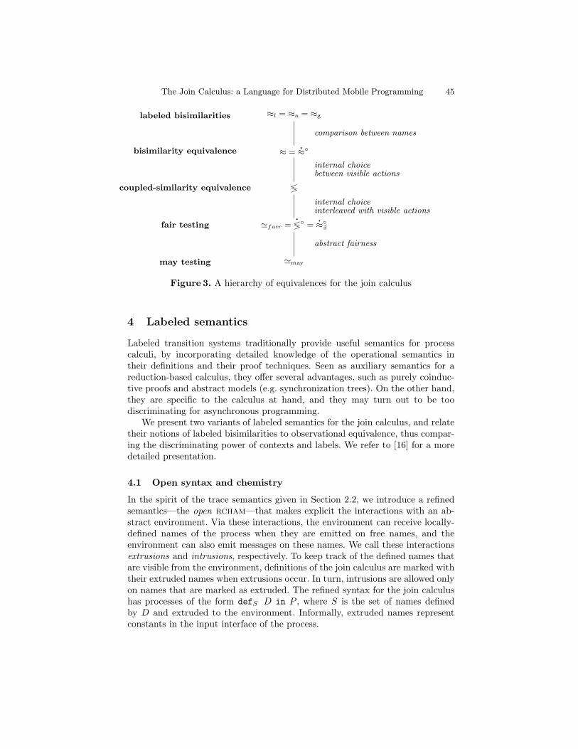
The Join Calculus: a Language for Distributed Mobile Programming 45
labeled bisimilarities ≈l = ≈a = ≈g
comparison between names
bisimilarity equivalence ≈ =.≈
internal choicebetween visible actions
coupled-similarity equivalence ≶
internal choiceinterleaved with visible actions
fair testing 'fair =.≶ =
.≈∃
abstract fairness
may testing 'may
Figure 3. A hierarchy of equivalences for the join calculus
4 Labeled semantics
Labeled transition systems traditionally provide useful semantics for processcalculi, by incorporating detailed knowledge of the operational semantics intheir definitions and their proof techniques. Seen as auxiliary semantics for areduction-based calculus, they offer several advantages, such as purely coinduc-tive proofs and abstract models (e.g. synchronization trees). On the other hand,they are specific to the calculus at hand, and they may turn out to be toodiscriminating for asynchronous programming.
We present two variants of labeled semantics for the join calculus, and relatetheir notions of labeled bisimilarities to observational equivalence, thus compar-ing the discriminating power of contexts and labels. We refer to [16] for a moredetailed presentation.
4.1 Open syntax and chemistry
In the spirit of the trace semantics given in Section 2.2, we introduce a refinedsemantics—the open rcham—that makes explicit the interactions with an ab-stract environment. Via these interactions, the environment can receive locally-defined names of the process when they are emitted on free names, and theenvironment can also emit messages on these names. We call these interactionsextrusions and intrusions, respectively. To keep track of the defined names thatare visible from the environment, definitions of the join calculus are marked withtheir extruded names when extrusions occur. In turn, intrusions are allowed onlyon names that are marked as extruded. The refined syntax for the join calculushas processes of the form defS D in P , where S is the set of names definedby D and extruded to the environment. Informally, extruded names representconstants in the input interface of the process.

46 Applied Semantics Summer School, Draft 7/01
A, B ::= open processesP plain process
|| defS D in P open definition|| A |B parallel composition
Figure 4. Syntax for the open join calculus
As a first example, consider the process def∅ x〈〉 . y〈〉 in z〈x〉. The interfacecontains no extruded name and two free names y, z. The message z〈x〉 can beconsumed by the environment, thus exporting x:
def∅ x〈〉 . y〈〉 in z〈x〉xz〈x〉−−−−−→ defx x〈〉 . y〈〉 in 0
Once x is known by the environment, it cannot be considered local anymore—theenvironment can emit on x—, but it is not free either—the environment cannotmodify or extend its definition. A new transition is enabled:
defx x〈〉 . y〈〉 in 0x〈〉−−→ defx x〈〉 . y〈〉 in x〈〉
Now the process can input more messages on x, and also perform the two tran-sitions below to consume the message on x and emit a message on y:
defx x〈〉 . y〈〉 in x〈〉 → defx x〈〉 . y〈〉 in y〈〉y〈〉−−−→ defx x〈〉 . y〈〉 in 0
We now extend the rcham of [14] with extrusions, intrusions, and explicit book-keeping of extruded names.
Definition 32. Open chemical solutions, ranged over by S, T , . . ., are triples(D, S,A), written D `S A, where D is a multiset of definitions, S is a subset ofthe names defined in D, and A is a multiset of open processes with disjoint setsof extruded names that are not defined in D.
The interface of an open solution S consists of two disjoint sets of free namesfv(S) and extruded names xv(S), defined in Figure 5. Functions dv(·), fv(·), andxv(·) are extended to multisets of terms by taking unions for all terms in themultisets.
The chemical rules for the open rcham are given in Figure 6; they definefamilies of transitions between open solutions , →, and α−→ where α rangesover labels of the form Sx〈v〉 and x〈v〉.
The structural rules and rule React are unchanged, but they now apply toopen solutions. Rule Str-Def performs the bookkeeping of exported names, andotherwise enforces a lexical scoping discipline with scope-extrusion for any namethat is not exported. When applied to open solutions, these structural rulescapture the intended meaning of extruded names: messages sent on extruded

The Join Calculus: a Language for Distributed Mobile Programming 47
In join patterns:rv(x〈v〉) = u ∈ v dv(x〈v〉) = xrv(J | J ′) = rv(J) ] rv(J ′) dv(J | J ′) = dv(J) ] dv(J ′)
In definitions:dv(J . P ) = dv(J) fv(J . P ) = dv(J) ∪ (fv(P )\rv(J))dv(D ∧ D′) = dv(D) ∪ dv(D′) fv(D ∧ D′) = fv(D) ∪ fv(D′)
In processes:fv(A |A′) = (fv(A) ∪ fv(A′)) \ (xv(A) ] xv(A′)) fv(0) = ∅xv(A |A′) = xv(A) ] xv(A′) xv(0) = ∅fv(defS D inA) = (fv(D) ∪ fv(A)) \ (dv(D) ] xv(A)) fv(x〈v〉) = x, vxv(defS D inA) = S ] xv(A) xv(x〈v〉) = ∅
In chemical solutions:fv(D `S A) = (fv(D) ∪ fv(A)) \ (dv(D) ] xv(A))xv(D `S A) = S ] xv(A)
Figure 5. Scopes in the open join calculus
Str-Null `S 0 `S
Str-Par `S A | A′ `S A, A′
Str-Top > `S `S
Str-And D ∧ D′ `S D, D′ `S
Str-Def `S defS′ D in A Dσ `S]S′ Aσ
React J . P `S Jρ → J . P `S Pρ
Ext `S x〈y〉 S′x〈y〉−−−−→ `S∪S′
Int `S∪xx〈y〉−−−→ `S∪x x〈y〉
Side conditions on the reacting solution S = (D `S A):in Str-Def, σ substitutes distinct fresh names for dv(D) \ S′;in React, ρ substitutes names for rv(J);in Ext, the name x is free, and S′ = y ∩ (dv(D) \ S);in Int, the names y are either free, or fresh, or extruded.
Figure 6. The open rcham

48 Applied Semantics Summer School, Draft 7/01
names can be moved inside or outside their defining process. For instance, wehave the structural rearrangement
`S x〈v〉 | defS′ D in A `S defS′ D in (x〈v〉 |A)
for any extruded name x, and as long as the names in v are not captured by D(v ∩ dv(D) ⊆ S′).
In addition, rules Ext and Int model interaction with the context. Accordingto rule Ext, messages emitted on free names can be received by the environment;these messages export any defined name that was not previously known to theenvironment, thus causing the scope of its definition to be opened. This is made
explicit by the set S′ in the label of the transitionS′x〈v〉−−−−→. Names in S′ must
be distinct from any name that appears in the interface before the transition;once these names have been extruded, they cannot be α-converted anymore, andbehave like constants. Our rule resembles the Open rule for restriction in thepi calculus [32], with an important constraint due to locality: messages are eitheremitted on free names, to be consumed by Ext, or on names defined in the opensolution, to be consumed by React.
The rule Int enables the intrusion of messages on exported names names. Itcan be viewed as a disciplined version of one of the two Input rules proposed byHonda and Tokoro for the asynchronous pi calculus, which enables the intrusionof any message [21]. The side condition of Int requires that intruded messagesdo not clash with local names of processes. (More implicitly, we may instead relyon the silent α-conversion on those local names; this is the original meaning of“intrusion” in [32].)
4.2 Observational equivalences on open terms
The notions of reduction-based equivalence defined in sections 2 and 3 are easilyextended to open processes, with the same definitions and the additional require-ment that related processes have the same exported names. (Indeed, it makeslittle sense to compare processes with incompatible interfaces such as 0 and theopen deadlocked solution defy x〈〉 | y〈〉 .in 0.) Context-closure properties arealso easily extended to take into account open contexts. Note that, whenever weapply a context, we implicitly assume that the resulting open process is well-formed. Finally, extrusions and strong barbs are in direct correspondence—we
have A ↓x if and only if ASx〈v〉−−−−→ A′ for any S,v, and A′.
In fact, the open syntax provides convenient notations to give selective giveaccess to some defined names in the processes being compared, but it does notintroduce any interesting new equation. Consider for instance bisimilarity equiv-alence on open terms:
Lemma 33. For all processes P1, P2 and definitions D1, D2, let x be a tupleof names defined in both D1 and D2, and let plug be a fresh name. The threefollowing statements are equivalent:
1. defx D1 in P1 ≈ defx D2 in P2

The Join Calculus: a Language for Distributed Mobile Programming 49
2. def D1 in P1 | plug〈x〉 ≈ def D2 in P2 | plug〈x〉3. for all D and P such that fv(def D in P ) ∩ (dv(D1) ∪ dv(D2)) ⊆ x and
dv(D)∩ (dv(D1)∪ dv(D2)) = ∅, we have def D ∧ D1 in P |P1 ≈ def D ∧D2 in P |P2.
The first formulation is the most compact; it relies on open terms. Instead, thesecond formulation makes explicit the communication of extruded names to theenvironment using a message on a fresh name plug; the third formulation isclosed by application of evaluation contexts, and is often used in direct proofsof bisimilarity equivalence (see for instance, [1]).
4.3 Labeled bisimulation
By design, the open join calculus can also be equipped with the standard notionof labeled bisimilarity:
Definition 34. A relation R on open processes is a labeled simulation if, when-ever A R B, we have
1. if A→ A′ then B →∗ B′ and A′ R B′;2. if A α−→ A′ then B →∗ α−→→∗ B′ and A′ R B′,
for all labels α of shape x〈v〉 or Sx〈v〉 such that fv(B) ∩ S = ∅.
A relation R is a labeled bisimulation when both R and R−1 are labeledsimulations. Labeled bisimilarity ≈l is the largest labeled bisimulation.
The simulation clause for intrusions makes weak bisimulation sensitive toinput interfaces: A ≈l B implies xv(A) = xv(B). The simulation clause for ex-trusion does not consider labels whose set of extruded names S clashes withthe free names of B, inasmuch as these transitions can never be simulated; thisstandard technicality does not affect the intuitive discriminating power of bisim-ulation, because names in S can be α-converted before the extrusion.
As opposed to contextual equivalences, it is possible to tell whether two pro-cesses are weakly bisimilar by comparing their labeled synchronization trees,rather than reasoning on their possible contexts. For example, x〈u〉 6≈l x〈v〉 be-cause each process performs an extrusion with distinct labels. Likewise, x〈y〉 6≈ldef z〈u〉 . y〈u〉 in x〈z〉 because the first process emits a free name (label x〈y〉)while the latter emits a local name that gets extruded (label zx〈z〉).
Besides, a whole range of “up to proof techniques” is available to reduce thesize of the relation to exhibit when proving labeled bisimilarities [30,33,39,41].For instance, one can reason up to other bisimilarities, or up to the restrictionof the input interface.
While its definition does not mention contexts, labeled bisimilarity is closedby application of any context:
Theorem 35. Weak bisimilarity is a congruence.

50 Applied Semantics Summer School, Draft 7/01
The proof is almost generic to mobile process calculi in the absence of externalchoice (see, e.g., [21,6] for the asynchronous pi calculus); it relies on two simplerclosure properties: ≈l is closed by application of evaluation contexts, and ≈l isclosed by renamings. We refer to [16] for the details.
As an immediate corollary, we can place labeled bisimilarity in our hierarchyof equivalence, and justify its use as an auxiliary proof technique for observationalequivalence: we have that ≈l is a reduction-based bisimulation that respectsall barbs and that is closed by application of contexts, hence ≈l ⊆ ≈. Thisinclusion is strict, as can be seen from the paradigmatic example of bisimilarityequivalence:
x〈z〉 ≈ def u〈v〉 . z〈v〉 in x〈u〉
That is, emitting a free name z is the same as emitting a bound name u thatforwards all the messages it receives to z, because the extra internal move forevery use of u is not observable. On the contrary, labeled bisimilarity separatesthese two processes because their respective extrusion labels reveal that z is freeand u is extruded. Since the contexts of the open join calculus cannot identifynames in messages, more powerful contexts are required to reconcile the twosemantics (see Section 4.5).
4.4 Asynchronous bisimulation
In order to prove that two processes are bisimilar, a large candidate bisimula-tion can be a nuisance, as it requires the analysis of numerous transition cases.Although they are not necessarily context-closed, labeled bisimulations on openchemical solutions are typically rather large. For example, a process with anextruded name has infinitely many derivatives even if no “real” computation isever performed. Consider the equivalence:
def x〈u〉 | y〈v〉 . P in z〈x〉 ≈l def x〈u〉 | y〈v〉 . Q in z〈x〉
These two processes are bisimilar because their join-pattern cannot be triggered,regardless of the messages the environment may send on x. Still, one is confrontedwith infinite models on both sides, with a distinct chemical solution for everymultiset of messages that have been intruded on x so far. This problem withlabeled bisimulation motivates an alternative formulation of labeled equivalence.
The join open rcham We modify the open rcham by allowing inputs onlywhen they immediately trigger a guarded process. For example, the two processesabove become inert after an extrusion xz〈x〉, hence trivially bisimilar. If weapplied this refinement with the same labels for input as before, however, wewould obtain a dubious result. The solution x〈〉 | y〈〉 | z〈〉 . P `x,y z〈〉 canprogress by first inputing two messages x〈〉 and y〈〉, then performing a silent stepthat consumes these two messages together with the local message z〈〉 alreadyin the solution. Yet, neither x〈〉 nor y〈〉 alone can trigger the process P , and

The Join Calculus: a Language for Distributed Mobile Programming 51
React-Int J . P `S MM′−−→ J . P `S Pρ
Side conditions:ρ substitute names for rv(J), Jρ ≡ M |M ′, and dv(M ′) ⊆ S.
The rules Str-(Null,Par,And,Def) and Ext are the same as in Figure 6.
Figure 7. The join open rcham
therefore this solution would become inert, too. This suggests the use of join-inputs on x and y in transitions such as
x〈〉 | y〈〉 | z〈〉 . P `x,y z〈〉x〈〉 | y〈〉−−−−−→ x〈〉 | y〈〉 | z〈〉 . P `x,y P
On the other hand, the solution x〈〉 | y〈〉 | z〈〉 . P `x z〈〉 is truly inert, sincethe environment has no access to y, and thus cannot trigger P . In this case, ourrefinement suppresses all input transitions.
The join open rcham is defined in Figure 7 as a replacement for the intrusionrule. In contrast with rule Int of Figure 6, the new rule React-Int permits theintrusion of messages only if these messages are immediately used to trigger aprocess. This is formalized by allowing labels M ′ that are parallel compositionsof messages. If the solution contains a complementary process M such thatthe combination M |M ′ matches the join-pattern of a reaction rule, then thetransition occurs and triggers this reaction rule. As for Int, we restrict intrusionsin M ′ to messages on extruded names.
We identify intrusions in the case M ′ = 0 with silent steps; the rule Reactis thus omitted from the new chemical machine. Nonetheless, we maintain thedistinction between internal moves and proper input moves in the discussion. Inthe sequel, we shall keep the symbol α−→ for the open rcham and use α−→J for thejoin open rcham; we may drop the subscript J when no ambiguity can arise.
Each open process now has two different models: for instance, the processdefx x〈〉 | y〈〉 . P in 0 has no transition in the join open rcham, while it has
infinite series of transitionsx〈〉−−→ x〈〉−−→ x〈〉−−→ · · · in the open rcham. A comparison
between the two transition systems yields the following correspondence betweentheir intrusions:
Proposition 36. Let A be an open process.
1. If Ax1〈v1〉 |··· | xn〈vn〉−−−−−−−−−−−→J B, then A
x1〈v1〉−−−−→ · · · xn〈vn〉−−−−→→ B.2. If A |x〈u〉 M−→J B and x ∈ xv(A), then
(a) either A M−→J A′ with A′ |x〈u〉 ≡ B;
(b) or AM | x〈u〉−−−−−→J B.
Accordingly, we adapt the definition of labeled bisimulation (Definition 34)to the new join open rcham. Consider the two processes:
Pdef= def x〈〉 . a〈〉 ∧ a〈〉 | y〈〉 . R in z〈x, y〉
Qdef= def x〈〉 | y〈〉 . R in z〈x, y〉

52 Applied Semantics Summer School, Draft 7/01
and assume a /∈ fv(R). With the initial open rcham, the processes P and Qare weakly bisimilar. With the new join open rcham and the same definitionof weak bisimulation, this does not hold because P can input x〈〉 after emittingon z while Q cannot. But if we consider the bisimulation that uses join-inputlabels instead of single ones, Q can input x〈〉 | y〈〉 while P cannot, and P and Qare still separated. It turns out that labeled bisimulation discriminates too muchin the join open rcham.
In order to retain an asynchronous semantics, labeled bisimulation must berelaxed, so that a process may simulate a React-Int transition even if it doesnot immediately consume all its messages. This leads us to the following defini-tion:
Definition 37. A relation R is an asynchronous simulation if, whenever A RB, we have
1. if ASx〈v〉−−−−→ A′ then B →∗ Sx〈v〉−−−−→→∗ B′ and A′ R B′
for all labels Sx〈v〉 such that fv(B) ∩ S = ∅;2. if A M−→ A′, then B | M →∗ B′ and A′ R B′;3. xv(A) = xv(B).
A relation R is an asynchronous bisimulation when both R and R−1 are asyn-chronous simulations. Asynchronous bisimilarity ≈a is the largest asynchronousbisimulation.
In the definition above, the usual clause for silent steps is omitted (it issubsumed by the clause for intrusions with M = 0). On the other hand, a clauseexplicitly requires that related solutions have the same extruded names.
Asynchronous bisimilarity and labeled bisimilarity do coincide. This validatesasynchronous bisimulation as an efficient proof technique.
Theorem 38. ≈a = ≈l.
To conclude our discussion on variants of labeled bisimulations, let us men-tion ground bisimulation, which is obtained by restricting the intrusions to labelsthat convey fresh names. As first observed in the pi calculus [21,6,8], asynchronybrings another interesting property as regards the number of transitions to con-sider: the ground variant of bisimilarities coincide with the basic one. This prop-erty also holds in the join calculus, thus providing proof techniques with, forevery chemical solution, exactly one intrusion per extruded name when usinglabeled bisimulation, and one intrusion per “active” partial join-pattern whenusing asynchronous bisimulation.
4.5 The discriminating power of name comparison
Labeled bisimilarity is finer than (reduction-based, barbed) bisimilarity equiva-lence and, as in other process calculi, these two semantics coincide only if we add

The Join Calculus: a Language for Distributed Mobile Programming 53
an operator for name comparisons [23,6]. In this section, we extend the syntaxof the join calculus accordingly, in the same style as [32].
Adef= . . . | [x=y]A P
def= . . . | [x=y]P
We also extend our chemical machines with a new reduction rule.
Compare `S [x=x]A → ` A
A technical drawback of this extension is that renamings do not preserve bisim-ilarity anymore. For instance, 0 ≈l [x=y]x〈〉, while after applying the renamingx/y, 0 6≈l [x=x]x〈〉. Accordingly, labeled bisimilarity is not a congruence any-more. For instance, the context C[·] def= def z〈x, y〉 . [·] in z〈u, u〉 separates 0and [x=y]x〈〉. We consider equivalences that are closed only by application ofevaluation contexts.
In the presence of comparisons, we still have:
Lemma 39. Labeled bisimilarity is closed by application of evaluation contexts
As regards observational equivalence, we let bisimilarity equivalence ≈be bethe largest barb-preserving bisimulation in the open join calculus with namecomparison that is closed by application of plain evaluation contexts. Bisimilarityequivalence now separates x〈z〉 from def u〈v〉 . z〈v〉 in x〈u〉 by using the contextdef x〈y〉 . [y=z] a〈〉 in [·], and labeled bisimilarity clearly remains finer thanbisimilarity equivalence. More interestingly, the converse inclusion also holds:
Theorem 40. With name comparison, we have ≈be = ≈l.
To establish the theorem, it suffices to show that, for every label, there is anevaluation context that specifically “captures” the label. Intrusions are very easy,since it suffices to use the parallel context x〈y〉 |[·]. Extrusions are more delicate,inasmuch as a context of the join calculus must define a name in order to detectan output transition on that name; this case is handled by creating a permanentrelay for all other messages on that name. Without additional care, this relaycan be detected by name matching, so we use instead a family of contexts thatseparate two aspects of a name. For every name x ∈ N , we let
Rx[·]def= def x〈y〉 . x′〈y〉 in vx〈x〉 |[·]
where the length of y matches the arity of x. Assuming x ∈ fv(A), the processRx[A] uses x′ as a free name instead of x, and forwards all messages from xto x′. The context should still be able to discriminate whether the process sendsthe name x or not by using name matching; this extra capability is suppliedin an auxiliary message vx〈x〉. The next lemma captures the essential propertyof Rx[·]:
Lemma 41 (Accommodating the extrusions). For all open processes Aand B such that x 6∈ xv(A) ∪ xv(B) and x′, vx are not in the interface of A andB, we have A ≈be B if and only if Rx[A] ≈be Rx[B].
54 Applied Semantics Summer School, Draft 7/01
Informally, the contexts Rx[·] are the residuals of contexts that test for labelsof the form Sx〈y〉. Once we have a context for every label, we easily provethat ≈be is a labeled bisimulation. Remark that the proof of the theorem wouldbe much harder if we were using the other notion of bisimilarity equivalence (seeSection 3.1), because we would have to characterize the whole synchronizationtree at once in a single context, instead of characterizing every label in isolation.This explains why many similar results in the literature apply only to processeswith image-finite transitions.
5 Distribution and mobility
Although distributed programming is the main purpose of the join calculus,the distribution of resources has been kept implicit so far. As we described itssemantics, we just argued that the join calculus had enough built-in locality tobe implemented in a distributed, asynchronous manner.
This section gives a more explicit account of distributed programming. Weextend the join calculus with locations and primitives for mobility. The resultingcalculus allows us to express mobile agents that can move between physical sites.Agents are not only programs but core images of running processes with theircommunication capabilities and their internal state. Inevitably, the resultingdistributed join calculus is a bit more complex than the core calculus of Section 1.
Intuitively, a location resides on a physical site, and contains a group ofprocesses and definitions. We can move atomically a location to another site.We represent mobile agents by locations. Agents can contain mobile sub-agentsrepresented by nested locations. Agents move as a whole with all their currentsub-agents, thereby locations have a dynamic tree structure. Our calculus treatslocation names as first class values with lexical scopes, as is the case for channelnames; the scope of every name may extend over several locations, and maybe dynamically extended as the result of message passing or agent mobility. Alocation controls its own moves, and can move towards another location by pro-viding the name of the target location, which would typically be communicatedonly to selected processes.
Since we use the distributed join calculus as the core of a programming lan-guage (as opposed to a specification language), the design for mobility is stronglyinfluenced by implementation issues. Our definition of atomic reduction stepsattempts to strike some balance between expressiveness and realistic concerns.Except for the (partial) reliable detection of physical failures, the refined opera-tional semantics has been faithfully implemented [18,12]. In these notes, however,we omit any specific discussion of these implementations.
5.1 Distributed mobile programming
We introduce the language with a few examples that assume the same approachto runtime distribution as in JoCaml. Execution occurs among several machines,

The Join Calculus: a Language for Distributed Mobile Programming 55
which may dynamically join or quit the computation; the runtime support con-sists of several system-level processes that communicate using TCP/IP. Processesand definitions can migrate from one machine to another but, at any given point,every process and definition of the language is running at a single machine.
From an asynchronous viewpoint, and in the absence of partial failures, lo-cality is transparent. Programs can be written independently of their runtimedistribution, and their visible results do not depend on their localization. In-deed, it is “equivalent” to run processes P and Q at different machines, or torun the compound process P |Q at a single machine. In particular, the scopes forchannel names and other values do not depend on their localization: whenever achannel appears in a process, it can be used to form messages (using the nameeither as the address, or as the message contents) without knowing whether thischannel is locally- or remotely-defined.
Of course, locality matters in some circumstances: side effects such as printingvalues on the local terminal depend on the current machine; besides, efficiencycan be affected as message-sending over the network takes much longer thanlocal calls; finally, the termination of some underlying runtime will affect allits local processes. For all these reasons, locality is explicitly controlled in thelanguage; this locality can be adjusted using migration. In contrast, resourcessuch as definitions and processes are not silently relocated or replicated by thesystem.
In JoCaml, programs being run on different machines do not initially shareany channel name; therefore, they would normally not be able to interact withone another. To bootstrap a distributed computation, it is necessary to exchangea few names; this is achieved using a built-in library called the name server. Oncethis is done, these names can be used to communicate some more names and tobuild more complex communication patterns. The interface of the name serverconsists of two functions to register and look up arbitrary values in a “globaltable” indexed by plain strings (JoCaml actually performs some dynamic typechecking at this stage). For instance, the process on the left below defines a localname cos and registers it to the name server:
def cos(x) = 1− x2/2 inNS.register(”cos”, cos)
def cos = NS.lookup(“cos′′) inprint(cos(0.1)); . . .
Using the same key “cos”, a remote program (such as the one on the right) canobtain the name cos then perform remote calls. The computation takes place onthe machine that defines cos (in the example, the machine hosting the programon the left).
More explicitly, the program defining cos may define a named location thatwraps this function definition, and may also export the location name under thekey “here”:
def here[cos(x) = 1− x2/2 :NS.register(“cos′′, cos); . . . ] in
NS.register(“here′′, here); . . .

56 Applied Semantics Summer School, Draft 7/01
The location definition does not affect cos, which can still be called locally or re-motely. In addition to remote access to cos, another program can now obtain thelocation name here, create locally a mobile sub-location—its “agent”—and relo-cate this agent to here. This makes sense, for instance, if the agent implementsprocesses that often call cos. The code on the client program may be:
def f(machine) .agent[
go machine;def cos = NS.lookup(”cos”) indef sum(s, n) = if n = 0 then s else sum(s+ cos(n), n− 1) inreturn sum(0, 10) ]
print(f(NS.lookup(”here”))); . . .
The new statement “go location;P” causes the enclosing location to migrate asa whole towards location’s machine before executing the following process P . Inthe program above, location agent migrates with its running process towardsthe machine that hosts here and cos, locally retrieves cos using the name serverand runs some computation, then eventually returns a single result to f ’s calleron the client machine.
A more complex example is an “applet server” that provides a function tocreate new instances of a library at a remote location provided by the caller. Tothis end, the server creates a mobile agent that wraps the instance of the library,migrates to the target location, and delivers the library interface once there. Forinstance, the code below implements a “one-place-buffer” library with some logmechanism:
def newOnePlaceBuffer(there) .def log(s) = print(”the buffer is ” + s) indef applet [
go there;def put(v) | empty〈〉 . log(”full”); (full〈v〉 | return)∧ get() | full〈v〉 . log(”empty”); (empty〈〉 | return v) in
empty〈〉 | return put , get to newBuf ] inlog(”created”); in
NS.register(”applet”, newOneP laceBuffer); . . .
A simple applet client may be:
def newBuf = NS.lookup(”newBuffer”) indef here[
def put , get = newBuf (here) input(1); . . . ] in . . .
In contrast with plain code mobility, the new applet can keep static access tochannels located at the applet server; in our case, every call to the one-placebuffer is local to the applet client, but also causes a remote log message to besent to the applet server.

The Join Calculus: a Language for Distributed Mobile Programming 57
5.2 Computing with locations
We now model locations and migrations as a refinement of the rcham. Weproceed in two steps. First, we partition processes and definitions into severallocal chemical solutions. This flat model suffices for representing both local com-putation on different sites and global communication between them. Then, weintroduce some more structure to account for the creation and the mobility oflocal solutions: we attach location names to solutions, and we organize them asa tree of nested locations. The refined syntax and chemical semantics appear infigures 8 and 9.
Distributed machines A distributed reflexive chemical machine (drcham) isa multiset of rchams. We write the global state of a drcham as several localsolutions D `α P connected by a commutative-associative operator ‖ thatrepresents distributed composition. Each local solution has a distinct label α—we will detail below the role of these labels.
Locally, every solution D `α P within a drcham evolves as before, accordingto the chemical rules given for the join calculus in Figure 2. Technically, thechemical context law is extended to enable computation in any local solution, andthe side condition in Str-Def requires that globally-fresh names be substitutedfor locally-defined names.
Two solutions can interact by using a new rule Comm that models globalcommunication. This rule states that a message emitted in a given solution α ona channel name x that is remotely defined can be forwarded to the solution βthat contains the definition of x. Later on, this message can be used within β toassemble a pattern of messages and to consume it locally, using a local Reactstep. This two-step decomposition of communication reflects the separation ofmessage transport and message processing in actual implementations.
In the following, we consider only drchams where every name is defined inat most one local solution. This condition is preserved by the chemical semantics,and simplifies the usage of rule Comm: for every message, the rule applies atmost once, and delivers the message to a unique receiving location. The actualmapping from channel names to their defining locations is static; it is maintainedby the implementation. (In contrast, some recent models of distributed systemsdetail the explicit routing of messages in the calculus [20,11]. From a languagedesign viewpoint, we believe that the bookkeeping of routing information is alow-level activity that is best handled at the implementation level. At least inthe distributed join calculus, the locality property makes routing informationsimple enough to be safely omitted from the language.)
Remote message passing To illustrate the use of several local solutions, wemodel a simplistic “print spooler” that matches available printers and job re-quests. The spooler can be described by the rule
Ddef= ready〈printer〉|job〈file〉 . printer〈file〉

58 Applied Semantics Summer School, Draft 7/01
A, B ::= configurationsD `ϕ P local solution (with path ϕ and contents D and P )
|| A ‖ B parallel composition
P, Q, R ::= processesx〈y〉 asynchronous message
|| go a; P migration request|| def D in P local definition|| P | Q parallel composition|| 0 inert process
D ::= join calculus definitionJ . P reaction rule
|| a [D : P ] sub-location (named a, with contents D and P )|| D ∧ D′ composition|| > void definition
J ::= join patternx〈y〉 message pattern
|| J | J ′ synchronization
Figure 8. Syntax for the distributed join calculus
Comm `α x〈y〉 ‖ D `β → `α ‖ D `β x〈y〉
Go `αa ‖ `βb go a; P → `αa ‖ `αab P
Str-Loc a[D : P ] `α D `αa P ‖ `α
Side conditions:in Comm, x ∈ dv(D);in Go, b does not occur in any other path;in Str-Loc, a does not occur in any other pathand D, P is the only content of solution αa.
The local rules are unchanged (cf. figure 2)distributed parallel composition ‖ is associate-commutative.
Figure 9. The distributed rcham

The Join Calculus: a Language for Distributed Mobile Programming 59
We assume that there are three machines: a user machine u that issues someprint request, a server machine s that hosts the spooler D, and a laser printer pthat registers to the spooler. We let P represent the printer code. We have theseries of chemical steps:
`u job〈1〉 ‖ D `s ‖ laser〈f〉 . P `p ready〈laser〉Comm→ `u ‖ D `s job〈1〉 ‖ laser〈f〉 . P `p ready〈laser〉Comm→ `u ‖ D `s job〈1〉, ready〈laser〉 ‖ laser〈f〉 . P `pReact→ `u ‖ D `s laser〈1〉 ‖ laser〈f〉 . P `pComm→ `u ‖ D `s ‖ laser〈f〉 . P `p laser〈1〉
The first step forwards the message job〈1〉 from the user machine u to the ma-chine that defines job, here the spooler s. Likewise, the second step forwards themessage ready〈laser〉 to the spooler. Next, synchronization occurs within thespooler between these two messages as a local reduction step. As a result, a newmessage on the spooler is sent to the laser printer, where it can be forwardedthen processed.
From this example, we can also illustrates global lexical scope. To model thatlaser is initially private to the printer machine p, we can use a preliminary local,structural step on machine p:
`p def laser〈f〉 . P in ready〈laser〉Str-def
laser〈f〉 . P `p ready〈laser〉
Then, the second Comm step in the series above extends the scope of laser tothe server, which gains the ability to send messages to the printer. In contrast,the scoping rules guarantees that no other process may send such messages atthis stage.
Nested locations Assuming that every location is mapped to its host machine,agent migration is naturally represented as an update of this mapping fromlocations to machines. For instance, a location that contains the running code ofa mobile agent may migrate to the machine that hosts another location providinga particular service.
Our model of locality is hierarchical, locations being attached to a parent lo-cation rather than a machine. A migration request is expressed using the processgo(a);P where a is the name of the target location and P is a guarded processtriggered after completing the migration. The migration is subjective, inasmuchas it applies to the location that runs the process go(a);P and its sublocations.
As regards distributed programming, there are many situations where sev-eral levels of moving resources are useful. For example, the server itself maysometimes move from one machine to another to continue the service while amachine goes down, and the termination of a machine and of all its locations canbe modeled using the same mechanisms as a migration. Also, some agents nat-urally make use of sub-agents, e.g., to spawn some parts of the computation toother machines. When a mobile agent returns to its client machine, for instance,

60 Applied Semantics Summer School, Draft 7/01
it may contain running processes and other resources; logically, the contents ofthe agent should be integrated with the client: later on, if the client moves, orfails, this contents should be carried away or discarded accordingly.
From the implementor’s viewpoint, the hierarchical model can be imple-mented as efficiently as the flat model, because each machine only has to keeptrack of its own local hierarchy of locations. Nonetheless, the model provides ad-ditional expressiveness to the programmer, who can assemble groups of resourcesthat move from one machine to another as a whole. This may explain why mostimplementations of mobile objects provide a rich dynamic structure for control-ling migration, for instance by allowing objects to be temporarily attached toone another (cf. [25,24]).
Consider for instance the case of concurrent migrations: a client creates anagent to go and get some information on a server; in parallel, the server goes toanother machine.
– With a flat location structure, the migration from the client to the servermust be dynamically resolved to a migration to a particular machine, e.g. themachine that currently hosts the server. In the case the server moves afterthe arrival of the agent, the agent is left behind. That is, the mapping fromlocations to machines depends on the scheduling of the different migrations,and the migration to the server yields no guarantee of being on the samemachine as the server.
– With a hierarchical structure, the ordering of nested migrations becomesirrelevant, and the agent is guaranteed to remain with the server as long asthe agent does not explicitly request another migration, even as the servermoves.
Relating locations to local chemical solutions We must represent locationsboth as syntactic definitions (when considered as a sublocation, or in a guardedprocess) and as local chemical solutions (when they interact with one another).We rely on location names to relate the two structures. We assume given acountable set of location names a, b, . . . ∈ L. We also write α, β, ab, αb, . . . ∈L∗ for finite strings of location names, or paths. Location names are first-classvalues. Much as channel names, they can be created locally, sent and received inmessages, and they have a lexical scope. To introduce new locations, we extendthe syntax of definitions with a new location constructor:
Ddef= . . . | a [D′ :P ]
where D′ gathers the definitions of the location, where P is the code running inthe location, and where a is a new name for the location. As regards the scopes,a [D′ :P ] defines the name a and the names defined in D′.
Informally, the definition a [D′ :P ] corresponds to the local solution D′ `βaP , where β is the path of D’s local solution. We say that `α is a sublocation of`β when β is a prefix of α. In the following, drchams are multisets of solutionslabeled with paths α that are all distinct, prefix-closed, and uniquely identified

The Join Calculus: a Language for Distributed Mobile Programming 61
by their rightmost location name, if any. These conditions ensure that solutionsordered by the sublocation relation form a tree.
The new structural rule Str-Loc relates the two representations of loca-tions. From left to right, the rule takes a sublocation definition and creates arunning location that initially contains a single definition D and a single runningprocess P . From right to left, Str-loc has a “freezing” effect on location a andall its sublocations. The rule has a side condition that requires that there is nosolution of the form `ψaφ in the implicit chemical context for any ψ, φ in L∗; incontrast, the definition D may contain sublocations. The side condition guaran-tees that D syntactically captures the whole subtree of sublocations in location awhen the rule applies. Note that the rule Str-def and its side condition alsoapply to defined location names. This guarantees that newly-defined locationsare given fresh names, and also that locations that are folded back into definingprocesses do not leave any running sublocation behind.
In well-formed drchams, we have required that all reaction rules defininga given channel name belong to a single local solution, and that all local solu-tions have distinct paths. With the addition of frozen locations in solution, wealso require that locations in solution all have distinct location names that donot appear in the path of any local solution. We constrain the syntax of defini-tions accordingly: in a well-formed definition, for all conjunctions D ∧ D′, werequire that dv(D) ∩ dv(D′) contain only port names that are not defined ina sublocation of D or D′. For instance, the definitions a [> :0] ∧ a [> :0] anda [x〈〉 . P ∧ b [x〈〉 . Q :0] :0] are ruled out.
As an example of nested locations, we describe a series of structural rear-rangements that enable some actual reduction steps. We assume that a does notoccur in Pc or Q.
` def c[x〈u〉 . Q ∧ a [Da :Pa] : Pc
]in y〈c, x〉|x〈a〉
Str-Def
c[x〈u〉 . Q ∧ a [Da :Pa] : Pc
]` y〈c, x〉|x〈a〉
Str-Loc
x〈u〉 . Q ∧ a [Da :Pa] `c Pc ` y〈c, x〉|x〈a〉Str-Def,Par
x〈u〉 . Q, a [Da :Pa] `c Pc ` y〈c, x〉, x〈a〉Str-loc
Da `ca Pa x〈u〉 . Q `c Pc ` y〈c, x〉, x〈a〉Comm→ Da `ca Pa x〈u〉 . Q `c Pc, x〈a〉 ` y〈c, x〉React→ Da `ca Pa x〈u〉 . Q `c Pc, Qa/u ` y〈c, x〉 ` def c
[x〈u〉 . Q : Pc|def a [Da :Pa] in Qa/u
]in y〈c, x〉
Now that the bookkeeping of the location tree is handled as a special case ofstructural rearrangement, we can express migration as the relocation of a branchin the location tree. We extend distributed chemical semantics with a secondreduction rule that operates on two chemical solutions (rule Go). Informally,location b moves from its current position βb in the tree to a new position αabjust under the location name a passed to the migration request. The targetsolution `αa is identified by its name a. Once b arrives, the guarded process P is

62 Applied Semantics Summer School, Draft 7/01
triggered. The side condition forces the preliminary application of rule Str-Locto fold any sublocation of a, and thus guarantees that the branch moves as awhole.
5.3 Attaching some meaning to locations
In the machine above, the locality structure is mostly descriptive: the distributedsemantics keeps track of locality information, but the location of a particular pro-cess or definition does not affect the result of the computation, at least for theobservables studied in Section 2. Formally, we can erase any locality informa-tion and relate the simple semantics to the distributed semantics. (Some care isrequired to rule out migration attempts towards one’s own sublocation, whichmay delay or block some processes.)
To conclude, we briefly present two refined models where locality has animpact on the computation and can be partially observed.
Partial failure and failure-detection Our calculus can be extended witha simple “fail-stop” model of failure, where the crash of a physical site causesthe permanent failure of its processes and definitions. In the extended model, alocation can halt with all its sublocations. The failure of a location can also beasynchronously detected at any other running location, allowing programmableerror recovery.
We supplement the syntax of distributed processes with constructs for failureand asynchronous failure detection:
P,Q,R ::= processes. . . (as in Figure 8)
|| halt local failure|| fail a;P remote failure detection
We also put an optional “has failed” marker Ω in front of every location namein paths, and add a side condition “the path does not contain Ω” in front ofevery chemical reduction rule (that is, a failed location and its sub-locationscannot migrate, communicate, or perform local steps). In addition, we providetwo chemical rules for the new constructs:
Halt `αa halt → `αΩa
Detect `αa ‖ `βb fail a;P → `αa ‖ `βb P
with side conditions: in Halt, a does not occur in any other path and themarker Ω does not occur in α; in Go, the marker Ω occurs in α but not in β.
Inasmuch as the only reported failures are permanent location failures, theprogramming model remains relatively simple4. For instance, the single delivery4 In addition, timeouts are pragmatically useful, but they are trivially modeled in
an asynchronous setting—they are ordinary non-deterministic reduction steps—andthey do not provide any negative guarantee.

The Join Calculus: a Language for Distributed Mobile Programming 63
of every message is guaranteed unless the sender fails, and thus the program-mer can consider larger units of failure. Besides, failure-detection provides usefulnegative information: once a location failure is detected, no other location mayinteract with it, hence its task may be taken over by another location without in-terfering with the failed location. The model of failure is only partially supportedin JoCaml (some failures may never be reported).
Authentication and Secrecy Interpreting locations as security boundaries,or “principals”, we have also developed a model of authentication for a variantof the join calculus [4]. In this variants, we consider only a flat and static parallelcomposition of locations.
As in the distributed join calculus, every name “belongs” to the single loca-tion that defines it, hence only that location can receive messages sent on thatname, while other locations cannot even detect those messages. In addition, ev-ery message carries a mandatory first parameter that contains a location name,meant to be the name of the sending location, and used by the receiver to au-thenticate the sender. These properties are both enforced by a modified Commrule:
Secure-Comm `a x〈c, y〉 ‖ Dx `b → `a ‖ Dx `b x〈a, y〉
where x is (uniquely) defined in Dx. Remark that the first parameter c is over-written with the correct sender identity a, much as in Modula 3’s secure networkobjects [42].
These secrecy and authenticity properties provide a strong, abstract ba-sis for reasoning on the security of distributed programs, but their semanticsdepends on global chemical conditions that are not necessarily met in practi-cal implementations—when communicating with an untrusted remote machine,there is no way to check that it is running a correct implementation. This deli-cate implementation is actually the main issue in [4], where we show that thosestrong properties can be faithfully implemented using standard cryptographicprimitives, with much weaker assumptions on the network. This result is ex-pressed in terms of bisimilarity equivalences.
Acknowledgements
These lecture notes are partly derived from previous works in collaborationwith Martın Abadi, Sylvain Conchon, Cosimo Laneve, Fabrice Le Fessant, Jean-Jacques Levy, Luc Maranget, Didier Remy, and Alan Schmitt.
References
1. M. Abadi, C. Fournet, and G. Gonthier. Secure implementation of channel abstrac-tions. Manuscript, on the Web at http://research.microsoft.com/~fournet;subsumes [2] and [3].

64 Applied Semantics Summer School, Draft 7/01
2. M. Abadi, C. Fournet, and G. Gonthier. Secure implementation of channel ab-stractions. In Proceedings of LICS ’98, pages 105–116. IEEE, June 1998.
3. M. Abadi, C. Fournet, and G. Gonthier. Secure communications processing fordistributed languages. In Proceedings of the 1999 IEEE Symposium on Securityand Privacy, pages 74–88, May 1999.
4. M. Abadi, C. Fournet, and G. Gonthier. Authentication primitives and their com-pilation. In Proceedings of POPL’00, pages 302–315. ACM, Jan. 2000.
5. G. Agha, I. Mason, S. Smith, and C. L. Talcott. A foundation for actor computa-tion. Journal of Functional Programming, 7(1):1–72, Jan. 1997.
6. R. M. Amadio, I. Castellani, and D. Sangiorgi. On bisimulations for the asyn-chronous π-calculus. Theoretical Computer Science, 195(2):291–324, 1998.
7. G. Berry and G. Boudol. The chemical abstract machine. Theoretical ComputerScience, 96:217–248, 1992.
8. M. Boreale and D. Sangiorgi. Some congruence properties for π-calculus bisimilar-ities. Theoretical Computer Science, 198(1–2):159–176, 1998.
9. E. Brinksma, A. Rensink, and W. Vogler. Fair testing. In I. Lee and S. A. Smolka,editors, 6th International Conference on Concurrency Theory (CONCUR’95), vol-ume 962 of LNCS, pages 313–327. Springer-Verlag, 1995.
10. E. Brinksma, A. Rensink, and W. Vogler. Applications of fair testing. InR. Gotzhein and J. Bredereke, editors, Formal Description Techniques IX: Theory,Applications and Tools, volume IX. Chapman and Hall, 1996.
11. L. Cardelli and A. Gordon. Mobile ambients. In Proceedings of FoSSaCS’98,volume 1378 of LNCS, pages 140–155. Springer-Verlag, 1998.
12. S. Conchon and F. Le Fessant. Jocaml: Mobile agents for objective-caml. InASA/MA’99, pages 22–29. IEEE Computer Society, Oct. 1999.
13. C. Fournet. The Join-Calculus: a Calculus for Distributed Mobile Programming.PhD thesis, Ecole Polytechnique, Palaiseau, Nov. 1998. INRIA TU-0556. Alsoavailable from http://research.microsoft.com/~fournet.
14. C. Fournet and G. Gonthier. The reflexive chemical abstract machine and thejoin-calculus. In Proceedings of POPL’96, pages 372–385. ACM, Jan. 1996.
15. C. Fournet and G. Gonthier. A hierarchy of equivalences for asynchronous calculi(extended abstract). In K. Larsen, S. Skyum, and G. Winskel, editors, Proceedingsof the 25th International Colloquium on Automata, Languages and Programming(ICALP ’98), volume 1443 of LNCS, pages 844–855, Aalborg, Denmark, July 1998.Springer-Verlag.
16. C. Fournet and C. Laneve. Bisimulations in the join-calculus. To appear in TCS,available from http://research.microsoft.com/~fournet, Oct. 2000.
17. C. Fournet, J.-J. Levy, and A. Schmitt. An asynchronous, distributed implementa-tion of mobile ambients. In J. van Leeuwen, O. Watanabe, M. Hagiya, P. Mosses,and T. Ito, editors, Proceedings of IFIP TCS 2000, volume 1872 of LNCS, Sendai,Japan, 17–19 Aug. 2000. IFIP TC1, Springer-Verlag. An extended report is avail-able from http://research.microsoft.com/~fournet.
18. C. Fournet and L. Maranget. The join-calculus language (version 1.03 beta).Source distribution and documentation available from http://join.inria.fr/,June 1997.
19. R. Glabbeek. The linear time—branching time spectrum II; the semantics of se-quential systems with silent moves (extended abstract). In E. Best, editor, 4thInternational Conference on Concurrency Theory (CONCUR’93), volume 715 ofLNCS, pages 66–81. Springer-Verlag, 1993. Also Manuscript, preliminary versionavailable at ftp://Boole.stanford.edu/pub/spectrum.ps.gz.
The Join Calculus: a Language for Distributed Mobile Programming 65
20. M. Hennessy and J. Riely. A typed language for distributed mobile processes. InProceedings of POPL ’98, pages 378–390. ACM, Jan. 1998.
21. K. Honda and M. Tokoro. On asynchronous communication semantics. In P. Weg-ner, M. Tokoro, and O. Nierstrasz, editors, Proceedings of the ECOOP’91 Work-shop on Object-Based Concurrent Computing, volume 612 of LNCS, pages 21–51.Springer-Verlag, 1992.
22. K. Honda and N. Yoshida. Combinatory representation of mobile processes. InProceedings of POPL ’94, pages 348–360, 1994.
23. K. Honda and N. Yoshida. On reduction-based process semantics. TheoreticalComputer Science, 152(2):437–486, 1995.
24. E. Jul. Migration of light-weight processes in emerald. IEEE Operating Sys. Tech-nical Committee Newsletter, Special Issue on Process Migration, 3(1):20, 1989.
25. E. Jul, H. Levy, N. Hutchinson, and A. Black. Fine-grained mobility in the emer-ald system. In Proceedings of the 11th ACM Symposium on Operating SystemsPrinciples, pages 62–74, November 1987.
26. C. Laneve. May and must testing in the join-calculus. Technical Report UBLCS96-04, University of Bologna, Mar. 1996. Revised: May 1996.
27. F. Le Fessant. The JoCAML system prototype (beta). Software and documentationavailable from http://pauillac.inria.fr/jocaml, 1998.
28. F. Le Fessant and L. Maranget. Compiling join-patterns. In U. Nestmann andB. C. Pierce, editors, HLCL ’98: High-Level Concurrent Languages, volume 16(3)of Electronic Notes in Theoretical Computer Science, Nice, France, Sept. 1998.Elsevier Science Publishers. To appear.
29. X. Leroy and al. The Objective CAML system 3.01. Software and documentationavailable from http://caml.inria.fr.
30. R. Milner. Communication and Concurrency. Prentice Hall, New York, 1989.31. R. Milner. Communication and Mobile Systems: the π-Calculus. Cambridge Uni-
versity Press, Cambridge, 1999.32. R. Milner, J. Parrow, and D. Walker. A calculus of mobile processes, parts I and
II. Information and Computation, 100:1–40 and 41–77, Sept. 1992.33. R. Milner and D. Sangiorgi. Barbed bisimulation. In W. Kuich, editor, Proceedings
of ICALP’92, volume 623 of LNCS, pages 685–695. Springer-Verlag, 1992.34. V. Natarajan and R. Cleaveland. Divergence and fair testing. In Proceedings of
ICALP ’95, volume 944 of LNCS. Springer-Verlag, 1995.35. U. Nestmann and B. C. Pierce. Decoding choice encodings. In U. Montanari and
V. Sassone, editors, 7th International Conference on Concurrency Theory (CON-CUR’96), volume 1119 of LNCS, pages 179–194. Springer-Verlag, Aug. 1996. Re-vised full version as report ERCIM-10/97-R051, 1997.
36. J. Parrow and P. Sjodin. Multiway synchronization verified with coupled simula-tion. In R. Cleaveland, editor, Third International Conference on ConcurrencyTheory (CONCUR’92), volume 630 of LNCS, pages 518–533. Springer-Verlag,1992.
37. J. Parrow and P. Sjodin. The complete axiomatization of cs-congruence. In P. En-jalbert, E. W. Mayr, and K. W. Wagner, editors, Proceedings of STACS’94, volume775 of LNCS, pages 557–568. Springer-Verlag, 1994.
38. D. Sangiorgi. Expressing Mobility in Process Algebras: First-Order and Higher-Order Paradigms. Ph.D. thesis, University of Edinburgh, May 1993.
39. D. Sangiorgi. On the bisimulation proof method. Revised version of TechnicalReport ECS–LFCS–94–299, University of Edinburgh, 1994. An extended abstractappears in Proc. of MFCS’95, LNCS 969, 1994.

66 Applied Semantics Summer School, Draft 7/01
40. D. Sangiorgi and R. Milner. The problem of “weak bisimulation up to”. In W. R.Cleaveland, editor, Proceedings of CONCUR’92, volume 630 of LNCS, pages 32–46.Springer-Verlag, 1992.
41. D. Sangiorgi and D. Walker. The Pi-calculus: a Theory of Mobile Processes. Cam-bridge University Press, July 2001. ISBN 0521781779.
42. L. van Doorn, M. Abadi, M. Burrows, and E. Wobber. Secure network objects. InProceedings of the 1996 IEEE Symposium on Security and Privacy, pages 211–221,May 1996.