The influence of macroeconomic developments on Austrian banks

BIS Papers No 1 91

The influence of macroeconomic developments on Austrian banks:implications for banking supervision

Markus Arpa, Irene Giulini, Andreas Ittner, Franz Pauer1

This paper aims to assess the effects of macroeconomic developments on risk provisions andearnings of Austrian banks for the 1990s. It seeks to detect economic indicators of potential instabilityin the banking system. The underlying theory is that bank earnings are to some extent directly (eg viainterest rates) and indirectly (eg via their customers) dependent on the state of the economy.

The main findings for the 1990s in Austria are as follows. Austrian banks increase risk provisions intimes of falling real GDP growth rates and in times of rising bank operating income or operatingresults. Net interest income appears to be uncorrelated with real GDP growth and interest ratedevelopments, with the exception that at very low interest rate levels net interest income shrinks. Forthe Austrian banking sector as a whole, falling short-term and long-term interest rates, along withrising real estate prices and/or inflation, push up bank operating income, and vice versa, which is inline with expectations. When breaking down the Austrian banking sector by peer groups, theexplanatory power of short-term interest rates becomes notably lower for most of the individual peergroups of the Austrian banking industry. The operating result of Austrian banks can be explained byand large by the same variables that explain their bank operating income. However, short-term interestrate developments are insignificant for the operating result, which suggests that - at least as far asdirect implications are concerned - monetary policy has been of minor significance for Austrian banksduring the last decade.

Overall, some macroeconomic variables such as interest rates, real estate and consumer prices canbe used to explain the income side, profitability and financial stability of Austrian banks. Structuralchanges, such as increased competition, joining the single market and the opening up of easternEuropean markets, have certainly also had a strong impact on Austrian banks. Furthermore, we drawthe conclusion that microeconomics, especially sound and prudent bank management - at least duringnormal (bank) business cycles - probably plays the major role in banking and supervision.

1.1 MotivationDuring the past two decades, many countries have experienced severe banking crises. Episodes ofprofound banking system distress have occurred not only in emerging and transition countries, butalso in advanced industrialised economies, such as the United States, the Nordic countries and morerecently Japan.2 In all cases, banking sector calamities have resulted in large losses of wealth and ledto disturbances in the credit supply to the economy. Resolving the crises has frequently imposed alarge burden on public funds.

The serious consequences mentioned above underline the value of indicators that signal a risingprobability of banking sector problems before such problems actually occur. They would provide auseful service for the purpose of banking supervision and financial market surveillance.

It is obvious that indicators relating directly to the soundness of the banking system are ideal for theprediction of banking crises. Items from banks’ balance sheets or profit and loss accounts shouldmake sufficiently clear when problems are becoming increasingly likely. There is no doubt that banks’earnings performance and the probability of banking system distress mainly depend on the conduct ofbusiness within banks, ie on micro factors. Inadequate accounting and auditing practices, insufficientinternal controls and poor management are the main causes for bank problems. In other words, bankcrises are mainly the result of bad banking. Adverse macroeconomic developments should not causesevere banking problems if the bank management acts farsightedly and reflects the cyclical nature of

1 The authors are at the Oesterreichische Nationalbank. We thank J Brockmeijer and W Waschiczek for valuable writtencomments as well as those colleagues at the Oesterreichische Nationalbank who commented in an internal discussionforum.

2 Austria has not experienced any systemic banking crises since the end of World War II.

92 BIS Papers No 1

the economy in its decisions. As this is not always the case, and because cyclical fluctuations aresometimes unexpectedly extreme, macroeconomic variables might well deliver good indicators for thelikelihood of mounting stress within the banking system.

1.2 How do macroeconomic developments influence the stability of the banking system?Although banking crises are mainly caused by microeconomic factors, disturbances anywhere in theeconomy are likely to have repercussions on the banking system. Due to the nature of their business,banks are exposed to many potential sources of distress rooted in cyclical developments. The mostdangerous characteristics in this respect are banks’ above average reliance on creditors’ funds(ie deposits) and their low capital ratio when compared to the corporate sector, their risky claims ondifferent sectors of the economy, and the fact that their assets are in effect longer-term and less liquidthan their liabilities. Banks’ health reflects to a large extent the health of their borrowers, which in turnreflects the health of the economy as a whole.

A useful way to analyse the macroeconomic determinants of banks’ health is to look at the main risksof banks: market risk (risk that values of underlying assets will decline), interest rate risk, exchangerate risk, default or credit risk (risk that debtors will be unable to repay their debts) and liquidity risk. Allthese risks are, at least partly, influenced by macroeconomic developments and policies.

An additional argument in favour of monitoring macroeconomic indicators for macroprudentialpurposes is the fact that the probability of systemic crises is greater when unsoundness is due tocyclical factors, because all banks are more or less exposed to the same conditions.

The evidence of past crises shows that certain macroeconomic variables typically display a distinctivepattern (boom and bust pattern) both before a banking crisis emerges and while it is unfolding. Ingeneral, the pattern is that of a rapid end to a boom: after rising rapidly, real GDP and domesticdemand decline; an acceleration in inflation is suddenly reversed; credit from the banking system tothe private sector builds up rapidly, peaks, and then contracts; real interest rates increase steadily, etc.

1.3 Development of production and domestic demand (cyclical indicators)Overall macroeconomic data on production and domestic demand provide information about the stateof the business cycle. The position of the cycle determines the earnings power of the public andprivate sectors and hence influences their debt servicing capability. When nourished by excessiveborrowing, buoyant production and demand growth can turn out to be the first phase of a boom-bustcycle, whose second phase is a sharp downturn which often causes debt servicing problems forborrowers. In the boom phase, debt servicing problems are comparatively rare due to the exceptionalearnings quality which tempts loan officers and bank managements to underestimate the riskiness oftheir business and reduce the margins of safety. Buoyant economic growth in combination withdeclining interest rate spreads gives a strong hint that such risky (mis)behaviour is widespread.

A swift and sharp decline in production, investment and consumption growth weakens the debtservicing capability of borrowers due to the declining financial surpluses of firms and reduced incomegrowth of households. In addition, the value of collateral (equity and real estate) usually fallsconsiderably in an economic slump, thus diminishing borrowers’ secondary means of servicing theirdebt. The accompanying fall in the value of collateral may aggravate the problems of adverseselection and moral hazard.3

Indicators selected

• Rate of growth in real GDP

− Exceptional growth rates may indicate a boom preceding a bust (indicator with a longlead).

3 Borrowers with low net worth constitute greater moral hazard to lenders, as they have less to lose at default. The less aborrower has to lose, the more he is inclined to engage in risky investments financed by bank loans.

BIS Papers No 1 93

− Sharply decelerating or negative growth rates point to an increased likelihood ofapproaching debt servicing problems.

• Rate of growth in nominal GDP

− As price developments often play a prominent or even dominant role in economicexcesses, changes in nominal GDP can provide additional information about changes inreal GDP.

• Rate of growth in real domestic demand

− Exceptional growth rates may indicate a boom (overinvestment and overconsumption)preceding a burst of the investment bubble and the consumption euphoria.

− Sharply decelerating or negative growth rates may point to beginning debt servicingproblems for companies and households.

• Rate of growth in nominal domestic demand

In this analysis we worked with real GDP and real domestic demand growth rates. Since themicroeconomic bank data in our analysis are always relative data (eg operating income relative to totalassets or risk provisions relative to total outstanding loans), we did not use nominal cyclical indicators.

1.4 Debt burden and leverage (financial fragility indicators)The soundness of the banking system crucially depends on the sustainability of the level of corporateand personal debt. If the private sector accumulates debt relative to assets beyond a critical level andshifts from borrowing adequately covered by cash flow to borrowing not covered, its debt servicingcapacity is likely to be impaired under worsening economic conditions. In addition to the increasedlikelihood of debt servicing problems, declining net worth of borrowers is also regarded (under thetheory of asymmetric information) as an incentive to moral hazard and adverse selection.

Whether and when borrowers with a high debt burden run into debt servicing problems essentiallydepends on the development of both interest payments and income. An increase in income gearing(interest payments as a proportion of income) caused either by declining earnings or rising interestpayments (due to rising interest rates and/or growing debt ratios) reduces the borrowers’ scope toservice their debt.

Indicators selectedThis type of indicator is not incorporated in this paper, since it is only available on an annual basis inAustria.

1.5 Excessive asset price developmentsPrices of certain assets can be very volatile, which makes the financing of their purchase or productiona risky business, sometimes involving heavy losses. The main reasons for the high volatility of certainasset prices are strong cyclical demand fluctuations (eg commodities), hog cycles due to longgestation periods (eg real estate) and speculative activity (eg shares). Inflated asset prices often leadbanks to make lending decisions based on asset values which are unsustainable in the long run. Inaddition, prudent creditors are likely to be driven into herding behaviour under such circumstances, asthey are undercut by those market participants disregarding the long-term risk involved in the loanfinancing of such assets.

Asset price slumps following excessive price hikes affect banks in various ways: first, they increaseborrowers’ indebtedness relative to their assets. This enhances the danger that borrowers may defaulton their payment obligations. Second, they reduce the value of banks’ own securities and real estateportfolios, which leads to capital losses. Third, due to negative wealth effects, the demand fromhouseholds and corporates may decline and hence accelerate the economic downturn.

94 BIS Papers No 1

Indicators selected

• Austrian and European share price indices

• Vienna real estate price index

− Due to myopic behaviour of (some) investors, a strong increase in real estate pricesattracts much more investment in new buildings than will be demanded at this high priceonce the bulk of the new property enters the market. This overinvestment tends to causethe price bubble to burst at some point and (all) real estate assets to decline in value,potentially leading to negative net worth of the property and debt servicing problems.

1.6 Monetary and financial conditionsBanking soundness to an important extent depends on the general monetary and financial conditions.Experience shows that banking crises often tend to be systemic when they are caused by deterioratingmonetary and financial conditions. The increase in (real) short-term interest rates has proved to be amajor source of systemic banking problems.

Indicators selected

• Monetary aggregates (M1 and M3)

− Accelerating money supply growth points to a potential overheating of the economy, whilesharply decelerating money supply growth can be, amongst other things, triggered by arecession and perhaps by deflationary effects in the economy, and/or it can be the resultof a restrictive monetary policy stance.

• Nominal and real short-term interest rates (three-month money market rate)

− High and rising short-term interest rates point to restrictive monetary policies, motivatedperhaps by an attempt to bring inflation under control. This imposes higher funding costs,while interest income cannot be increased equivalently as the interest rate for the stock ofloans is usually fixed for a longer period. Furthermore, high short-term interest rates arelikely to hurt banks even if they can be passed on to borrowers in the form of high lendingrates. The reason is the tendency for adverse selection, which can increase theproportion of non-performing loans in the medium and long run.

• Nominal and real long-term interest rates (five-year benchmark government bond)

− Investment project decisions depend on the long-term interest rate. Normally, an internalrate of return is used to test whether investment projects are worth undertaking. Risinglong-term interest rates may push projects with an initial positive value towards a negativevalue on account of the new internal rate of return.

− Besides the credit risk, the long-term interest rate affects the return on bank securities,and therefore it also imposes a market risk on the sector.

• Overall interest rate margin (average interest rate on banks’ assets minus average interestrate on banks’ liabilities)

− Competition may cause banks to make inadequate provisions for detrimental events suchas asset price collapses or cyclical downturns, because banks that make adequateprovisions are undercut by those disregarding such possibilities for reasons of ignoranceor competitive advantage.

• Rate of inflation (consumer price index)

− High inflation rates usually go hand in hand with high nominal interest rates and willeventually lead to high real interest rates, which reduce the profitability of credit-financedinvestment projects and increases income gearing in real terms. However, rising inflationmay temporarily reduce the real value of (fixed) interest payments by firms, thusincreasing profitability for a certain period of time. Generally, a high and volatile nominalinterest rate associated with high inflation makes it difficult for banks to perform maturity

BIS Papers No 1 95

transformation. High rates of inflation may proxy for macroeconomic mismanagement,which adversely affects the economy and the banking sector through various channels.

1.7 Bank dataThe micro bank data used for this paper are taken from the monthly raw balance sheet and thequarterly income statement which Austrian banks have to report to the supervisory authority and thecentral bank. These data are delivered on an unconsolidated basis, ie including domestic branchoffices and branch offices abroad, but excluding bank and other subsidiaries.

Risk provisions are calculated as total provisions for loans granted to banks and non-banks as apercentage of total loans plus total provisions for loans. This ratio is not taken from audited financialstatements (which are available only on an annual basis), since this would not have generated enoughobservations for our statistical analysis. Therefore, these figures are taken from the monthly rawbalance sheets. This implies, as the name already suggests, that the extent of provisions as auditedby external auditors at the end of the year might deviate from the figures used for this analysis.

As regards income figures, we based our analysis on the following breakdown:

Interest income– Interest expense= NET INTEREST INCOME+ income from securities+ net income from fees and commissions+ net profit (loss) on financial operations+ other operating income= OPERATING INCOME– operating expenses= OPERATING RESULT– RISK PROVISIONS– taxes+/– extraordinary items= PROFIT

Income from securities includes income from shares and other variable yield securities, income fromparticipating interests and income from shares in affiliated companies.

Operating expenses include personnel and other administrative expenses, value adjustments onintangible and tangible fixed assets (such as land and buildings), but exclude value adjustments forloans and securities. Therefore, both operating income and the operating result do not includeprovisions for loan losses or for losses on securities.

Our analysis is based on net quarterly data, ie data on the second quarter do not include data from thefirst quarter in any given year.

For the purpose of supervisory analysis, Austrian banks are grouped into peer groups, according tothe structure of their assets. Some banks, due to their special status, had to be classified in specialgroups heuristically (ie by conceptual assumption) a priori.

− All large banks with total assets exceeding EUR 2 billion were placed in Peer Group 1. Thetotal assets of this peer group amount to nearly three quarters of the total assets of allAustrian banks.

− All foreign banks (foreign assets of more than 30% of total assets) that do not come underthe group of large banks constitute Peer Group 2.

− All specialised banks (those of the special purpose bank sector, including building and loanassociations, etc) were grouped into Peer Group 3.

− The remaining banks were classified according to their balance sheet structure. Theliabilities side of the balance sheet proved too blunt an instrument for differentiation; notablybecause savings deposits tend to correlate strongly with the balance sheet total, thisbreakdown would have been too close to the total asset criterion. Therefore, it was decidedto use the assets side as a grouping criterion. Except for off-balance sheet business, theassets side reflects a bank’s risk potential fairly accurately. The relation between domestic

96 BIS Papers No 1

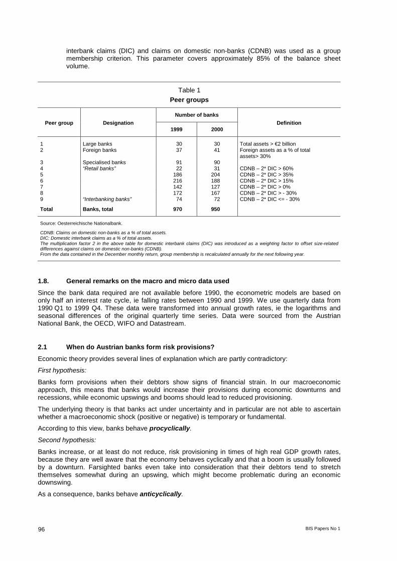
interbank claims (DIC) and claims on domestic non-banks (CDNB) was used as a groupmembership criterion. This parameter covers approximately 85% of the balance sheetvolume.

Table 1Peer groups

Number of banksPeer group Designation

1999 2000Definition

1 Large banks 30 30 Total assets > €2 billion2 Foreign banks 37 41 Foreign assets as a % of total

assets> 30%3 Specialised banks 91 904 “Retail banks” 22 31 CDNB – 2* DIC > 60%5 186 204 CDNB – 2* DIC > 35%6 216 188 CDNB – 2* DIC > 15%7 142 127 CDNB – 2* DIC > 0%8 172 167 CDNB – 2* DIC > - 30%9 “Interbanking banks” 74 72 CDNB – 2* DIC <= - 30%

Total Banks, total 970 950

Source: Oesterreichische Nationalbank.

CDNB: Claims on domestic non-banks as a % of total assets.DIC: Domestic interbank claims as a % of total assets.The multiplication factor 2 in the above table for domestic interbank claims (DIC) was introduced as a weighting factor to offset size-relateddifferences against claims on domestic non-banks (CDNB).From the data contained in the December monthly return, group membership is recalculated annually for the next following year.

1.8. General remarks on the macro and micro data usedSince the bank data required are not available before 1990, the econometric models are based ononly half an interest rate cycle, ie falling rates between 1990 and 1999. We use quarterly data from1990 Q1 to 1999 Q4. These data were transformed into annual growth rates, ie the logarithms andseasonal differences of the original quarterly time series. Data were sourced from the AustrianNational Bank, the OECD, WIFO and Datastream.

2.1 When do Austrian banks form risk provisions?Economic theory provides several lines of explanation which are partly contradictory:

First hypothesis:

Banks form provisions when their debtors show signs of financial strain. In our macroeconomicapproach, this means that banks would increase their provisions during economic downturns andrecessions, while economic upswings and booms should lead to reduced provisioning.

The underlying theory is that banks act under uncertainty and in particular are not able to ascertainwhether a macroeconomic shock (positive or negative) is temporary or fundamental.

According to this view, banks behave procyclically.

Second hypothesis:

Banks increase, or at least do not reduce, risk provisioning in times of high real GDP growth rates,because they are well aware that the economy behaves cyclically and that a boom is usually followedby a downturn. Farsighted banks even take into consideration that their debtors tend to stretchthemselves somewhat during an upswing, which might become problematic during an economicdownswing.

As a consequence, banks behave anticyclically.

BIS Papers No 1 97

Third hypothesis:

Banks increase risk provisions when they engage in riskier business. This might well be correlatedwith higher returns, ie increased operating income for banks, since riskier business should lead tohigher returns on average.

Fourth hypothesis:

Banks increase risk provisions in times of rising operating returns. This behaviour is partly connectedto the behaviour described under hypothesis three, since operating return is defined as operatingincome minus operating expenses and therefore depends to some extent on returns.

Another argument for this type of behaviour is the attempt of banks to reduce the income tax burdenby evening out profits and losses over time. Another, somewhat similar, reasoning is that banks wantto produce a constant income stream, perhaps in order to generate trust among the public. Therefore,banks generally aim to reduce the volatility of their net income.

However, some banks might increase risk provisions simply when they can “afford” to do so,depending amongst other things on accounting standards and supervisory rules.

Econometric models:

We tested different multiple regression models to assess which of the above-mentioned explanationscomes closest to the behaviour of Austrian banks.

In our models, risk provisions are defined as a percentage of total outstanding loans. For1995 Q4-1996 Q3, a dummy variable (D96) has been used, due to a change in the definition of riskprovisions in per cent of total outstanding loans by December 1995.

Test of the first hypothesis:

First, we formulated a multiple regression model in the form of (all variables in log and seasonallyadjusted)

Provisions = c + b1 * GDP(r) + b2 * RealEstateLag2Q + b3 * RealInterestRate3M + b4 * D96.

Changes in risk provisions relative to total loans depend on real GDP growth rates, real estate pricedevelopments (lagged by two quarters), the development of real interest rates (three-month moneymarket rate minus annual inflation rate) and the dummy variable. Asset prices, like real estate prices,obviously play a role in risk provisions, since the underlying assets are often used as mortgage. Sincereal estate price developments and their possible implications for loan provisioning become visibleonly with a certain time lag, we lagged this time series by two quarters.

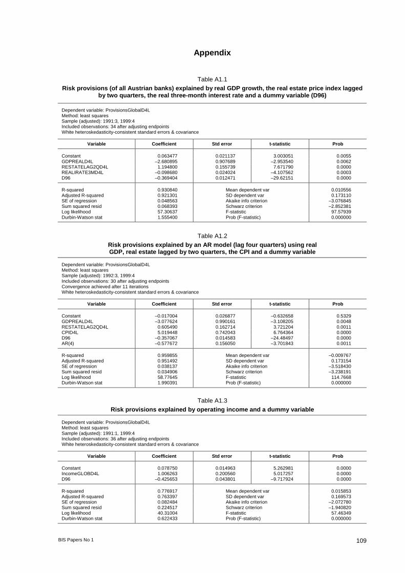
This model delivers a good proxy. All variables are highly significant, the explanatory power of themodel is very high (adjusted R² of 0.92), and we experience only low positive autocorrelation(Durbin-Watson: 1.6). According to this model, risk provisions rise when real GDP growth declines(procyclical behaviour), they rise when real estate prices rise (anticyclical behaviour), and theyrise when real interest rates fall (see Table A1.14).

Since risk provisions of all Austrian banks significantly depend negatively on real GDP growth,Austrian banks behave procyclically when it comes to forming risk provisions.

The sign of the first independent variable (real GDP growth) confirms the first hypothesis mentionedabove, but the sign of the second independent variable, real estate prices, is questionable. Whenreal estate prices rise, banks should be relieved as the value of mortgages rises, because this shouldreduce the likelihood of loan losses and therefore provisioning for real estate loans. Conversely,declining real estate prices should set bells ringing at banks, as the value of their mortgages declinesand the chance that they may suffer a loss in the case of debt service problems of borrowers rises.However, it cannot be ruled out - even though we regard it as less likely - that banks behave“anticyclically” when it comes to real estate developments. In general, we are somewhat hesitant toaccept that the Vienna real estate price index should have such a significant influence on riskprovisions.

4 Table numbers prefixed by an A can be found in the Appendix.

98 BIS Papers No 1

Rising real interest rates should indicate growing financial strains in an economy. Rising real interestrates tend to increase financial fragility via an increase in the interest service burden for debtors, whichshould be reflected in banks’ risk provisions. On the other hand, rising real interest rates are typical fortimes of (prolonged) strong economic growth, while falling real interest rates are typical for the earlystages of an economic trough and during recessions.

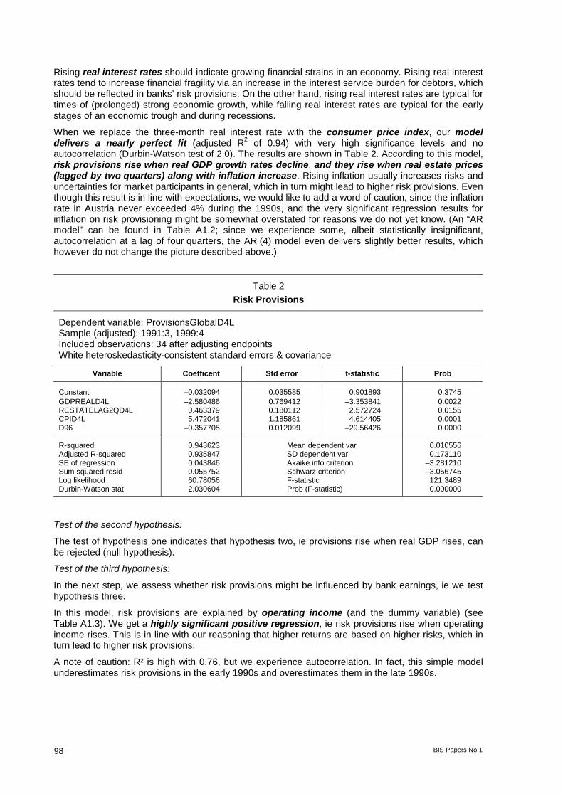
When we replace the three-month real interest rate with the consumer price index, our modeldelivers a nearly perfect fit (adjusted R2 of 0.94) with very high significance levels and noautocorrelation (Durbin-Watson test of 2.0). The results are shown in Table 2. According to this model,risk provisions rise when real GDP growth rates decline, and they rise when real estate prices(lagged by two quarters) along with inflation increase. Rising inflation usually increases risks anduncertainties for market participants in general, which in turn might lead to higher risk provisions. Eventhough this result is in line with expectations, we would like to add a word of caution, since the inflationrate in Austria never exceeded 4% during the 1990s, and the very significant regression results forinflation on risk provisioning might be somewhat overstated for reasons we do not yet know. (An “ARmodel” can be found in Table A1.2; since we experience some, albeit statistically insignificant,autocorrelation at a lag of four quarters, the AR (4) model even delivers slightly better results, whichhowever do not change the picture described above.)

Table 2Risk Provisions

Dependent variable: ProvisionsGlobalD4LSample (adjusted): 1991:3, 1999:4Included observations: 34 after adjusting endpointsWhite heteroskedasticity-consistent standard errors & covariance

Variable Coefficent Std error t-statistic Prob

Constant –0.032094 0.035585 0.901893 0.3745GDPREALD4L –2.580486 0.769412 –3.353841 0.0022RESTATELAG2QD4L 0.463379 0.180112 2.572724 0.0155CPID4L 5.472041 1.185861 4.614405 0.0001D96 –0.357705 0.012099 –29.56426 0.0000

R-squared 0.943623 Mean dependent var 0.010556Adjusted R-squared 0.935847 SD dependent var 0.173110SE of regression 0.043846 Akaike info criterion –3.281210Sum squared resid 0.055752 Schwarz criterion –3.056745Log likelihood 60.78056 F-statistic 121.3489Durbin-Watson stat 2.030604 Prob (F-statistic) 0.000000

Test of the second hypothesis:

The test of hypothesis one indicates that hypothesis two, ie provisions rise when real GDP rises, canbe rejected (null hypothesis).

Test of the third hypothesis:

In the next step, we assess whether risk provisions might be influenced by bank earnings, ie we testhypothesis three.

In this model, risk provisions are explained by operating income (and the dummy variable) (seeTable A1.3). We get a highly significant positive regression, ie risk provisions rise when operatingincome rises. This is in line with our reasoning that higher returns are based on higher risks, which inturn lead to higher risk provisions.

A note of caution: R² is high with 0.76, but we experience autocorrelation. In fact, this simple modelunderestimates risk provisions in the early 1990s and overestimates them in the late 1990s.

BIS Papers No 1 99

Test of the fourth hypothesis:

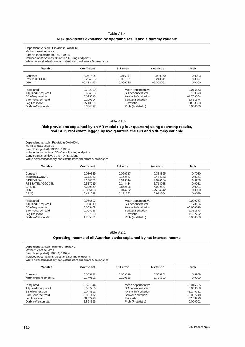
Now we explain risk provisions by operating result (see Table A1.4). Again, we find a significantpositive link. Since the operating result is defined as operating income minus operating expenses, itis not surprising that the significant positive link of operating income with risk provisions is also foundin this model.

Because the explanatory power of the operating result is somewhat less significant (andautocorrelation even higher), we are inclined to argue that risk provisions can be explained better byoperating income than by the operating result. However, it cannot be ruled out that banks tend toincrease their risk provisions in “good times”, ie because the bank operating result is high. Whetherthis type of behaviour is mainly triggered by tax or by confidence considerations, or perhapssomething else, is difficult to assess.

To summarise these results, Austrian banks appear to behave procyclically, ie they increase riskprovisions in times of declining real GDP growth rates. In addition, Austrian banks form risk provisionswhen their operating income rises. It cannot be ruled out that banks form risk provisions because theoperating result rises. The model also delivers the result that rising inflation and rising real estateprices lead to higher risk provisions. While the first result is in line with expectations, even though it issomewhat astonishing that relatively moderate inflation rates have such a significant impact on riskprovisioning, the latter result is not in line with expectations.

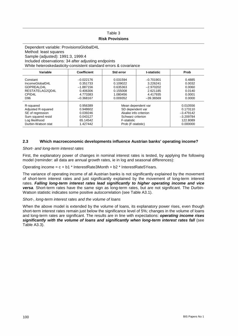
Putting the above findings in a single model delivers the expected result; see Table 3 and Figure 1.The statistical tests highlight that the explanatory power of this model with an adjusted R² of 0.95 andvery high significance levels is exceptionally high (see table and corresponding Figure below). (TheDurbin-Watson statistic indicates autocorrelation; however a close analysis of the residuals comes tothe conclusion that the autocorrelation of the residuals is statistically not significant (probabilityvalues ≥ 0.15) and therefore does not pose a problem. Nevertheless, for an AR(4) model which dealswith this insignificant autocorrelation, see Table A1.5.)

2.2 What determines net interest income?Austrian banks’ operating income (still) very much depends on net interest income. This is alsoconfirmed by a simple regression analysis, where operating income is very well explained by netinterest income (see Table A2.1).

According to our multiple regression analysis, net interest income is not well explained by marketshort- and long-term interest rate developments and appears to be uncorrelated with real GDPgrowth (see Table A2.2; very much the same holds if net interest income is lagged by one year versusinterest rate developments). However, we cannot rule out that net interest income reacts to interestrate developments with a very long time lag of perhaps three or four years. Since our data cover only10 years, a time lag of that magnitude leads to serious econometric problems and could not be testedby us.

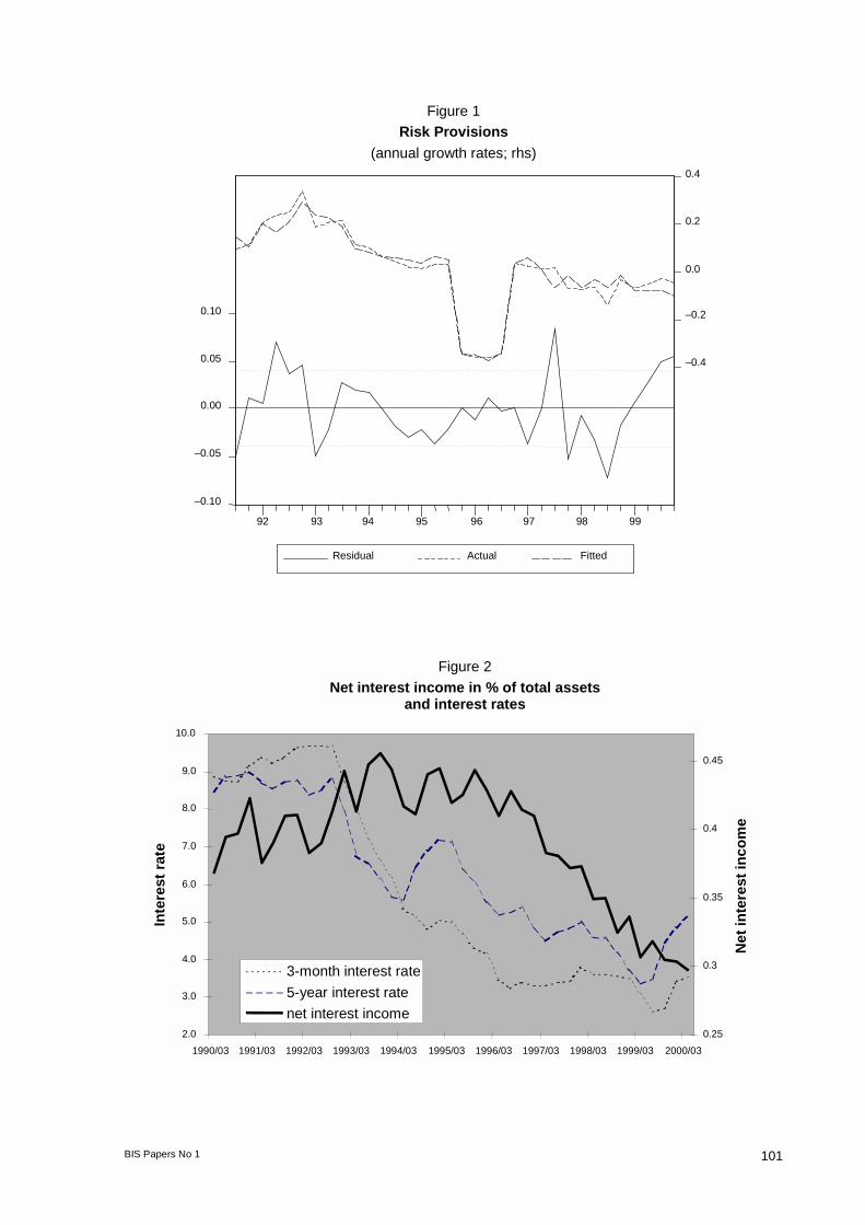
Anecdotal evidence as well as a graphic analysis of recent net interest developments in Austria leadus to the conclusion that the level of interest rates most likely has some influence on net interestincome (see Figure 2). When short-term interest rates (three-month money market rates) hoveredaround or below 3.5%, and long-term interest rates (five-year government bonds) fell below 5%, netinterest income started to fall (with a certain time lag). This might be explained by the fact that interestrates for customer deposits reached a point where they could not fall much further (eg in the case ofretail overnight deposits), and/or customers started to move to other, higher-yield forms of investment(eg mutual funds). In the latter case, banks had to refinance themselves in other, usually moreexpensive ways (eg via money markets and bonds). On the other side of the balance sheet, interestrates for loans still had room to go down further and low rates were attractive for debtors. This causedthe spread between active and passive interest rates to narrow.

100 BIS Papers No 1

Table 3Risk Provisions

Dependent variable: ProvisionsGlobalD4LMethod: least squaresSample (adjusted): 1991:3, 1999:4Included observations: 34 after adjusting endpointsWhite heteroskedasticity-consistent standard errors & covariance

Variable Coefficient Std error t-statistic Prob

Constant –0.022176 0.031594 –0.701901 0.4885IncomeGlobalD4L 0.351733 0.109022 3.226241 0.0032GDPREALD4L –1.887156 0.635363 –2.970202 0.0060RESTATELAG2QD4L 0.406306 0.155008 2.621185 0.0140CPID4L 4.773383 1.080456 4.417935 0.0001D96 –0.368167 0.009352 –39.36569 0.0000


2.3 Which macroeconomic developments influence Austrian banks’ operating income?Short- and long-term interest rates

First, the explanatory power of changes in nominal interest rates is tested, by applying the followingmodel (reminder: all data are annual growth rates, ie in log and seasonal differences):

Operating income = c + b1 * InterestRate3Month + b2 * InterestRate5Years.

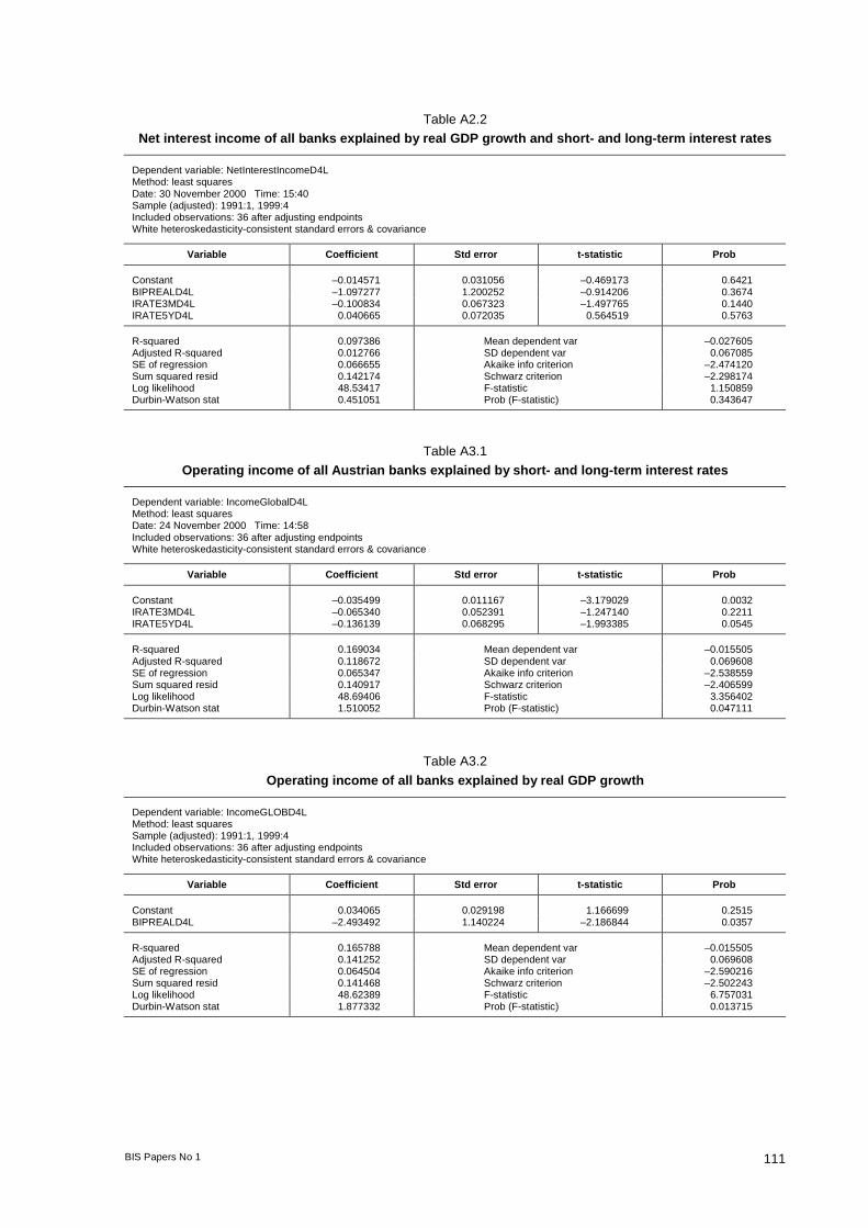
The variance of operating income of all Austrian banks is not significantly explained by the movementof short-term interest rates and just significantly explained by the movement of long-term interestrates. Falling long-term interest rates lead significantly to higher operating income and viceversa. Short-term rates have the same sign as long-term rates, but are not significant. The Durbin-Watson statistic indicates some positive autocorrelation (see Table A3.1).

Short-, long-term interest rates and the volume of loans

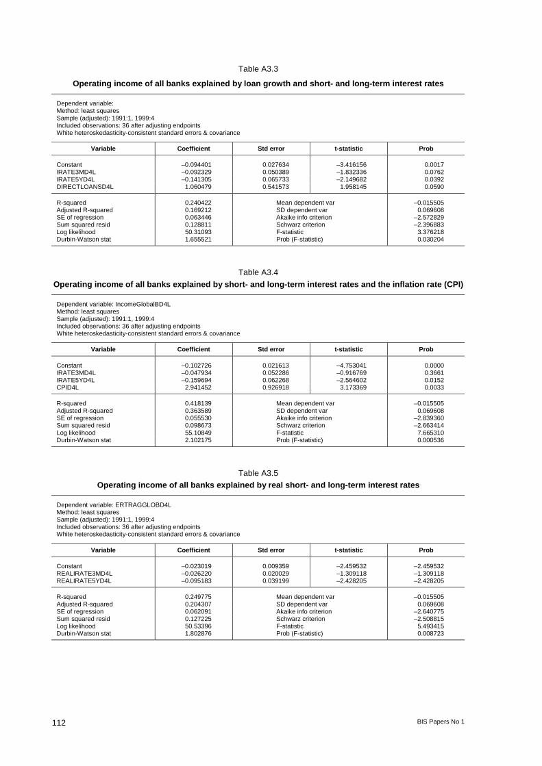
When the above model is extended by the volume of loans, its explanatory power rises, even thoughshort-term interest rates remain just below the significance level of 5%; changes in the volume of loansand long-term rates are significant. The results are in line with expectations: operating income risessignificantly with the volume of loans and significantly when long-term interest rates fall (seeTable A3.3).

BIS Papers No 1 101

Figure 1Risk Provisions

(annual growth rates; rhs)

–0.10

–0.05

0.00

0.05

0.10

–0.4

–0.2

0.0

0.2

0.4

92 93 94 95 96 97 98 99

Residual Actual Fitted

Figure 2Net interest income in % of total assets

and interest rates

2.0

3.0

4.0

5.0

6.0

7.0

8.0

9.0

10.0

1990/03 1991/03 1992/03 1993/03 1994/03 1995/03 1996/03 1997/03 1998/03 1999/03 2000/03

Inte

rest

rate

0.25

0.3

0.35

0.4

0.45

Net

inte

rest

inco

me

3-month interest rate5-year interest ratenet interest income

102 BIS Papers No 1

Short-, long-term interest rates and real estate prices

In this model we use real estate prices in Vienna, lagged by two quarters, as one of the explanatoryvariables. A lag of two quarters is introduced, since it certainly takes time before real estate pricedevelopments and their effects on customers (loans, etc) show up in bank income. Lagging this realestate index by four quarters leads to similar but somewhat less significant results.

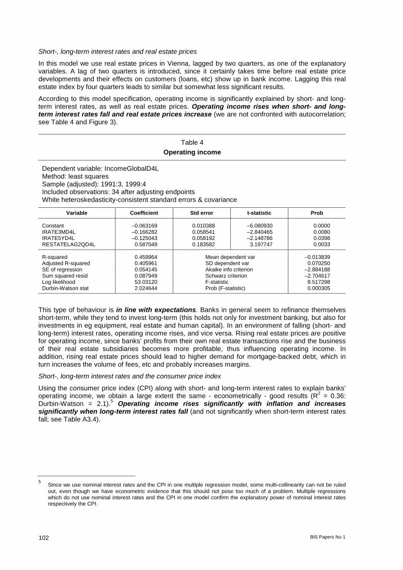
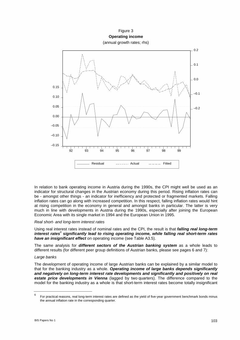
According to this model specification, operating income is significantly explained by short- and long-term interest rates, as well as real estate prices. Operating income rises when short- and long-term interest rates fall and real estate prices increase (we are not confronted with autocorrelation;see Table 4 and Figure 3).

Table 4Operating income

Dependent variable: IncomeGlobalD4LMethod: least squaresSample (adjusted): 1991:3, 1999:4Included observations: 34 after adjusting endpointsWhite heteroskedasticity-consistent standard errors & covariance


Constant –0.063169 0.010388 –6.080930 0.0000IRATE3MD4L –0.166282 0.058541 –2.840465 0.0080IRATE5YD4L –0.125043 0.058192 –2.148786 0.0398RESTATELAG2QD4L 0.587049 0.183582 3.197747 0.0033

R-squared 0.459964 Mean dependent var –0.013839Adjusted R-squared 0.405961 SD dependent var 0.070250SE of regression 0.054145 Akaike info criterion –2.884188Sum squared resid 0.087949 Schwarz criterion –2.704617Log likelihood 53.03120 F-statistic 8.517298Durbin-Watson stat 2.024644 Prob (F-statistic) 0.000305

This type of behaviour is in line with expectations. Banks in general seem to refinance themselvesshort-term, while they tend to invest long-term (this holds not only for investment banking, but also forinvestments in eg equipment, real estate and human capital). In an environment of falling (short- andlong-term) interest rates, operating income rises, and vice versa. Rising real estate prices are positivefor operating income, since banks’ profits from their own real estate transactions rise and the businessof their real estate subsidiaries becomes more profitable, thus influencing operating income. Inaddition, rising real estate prices should lead to higher demand for mortgage-backed debt, which inturn increases the volume of fees, etc and probably increases margins.

Short-, long-term interest rates and the consumer price index

Using the consumer price index (CPI) along with short- and long-term interest rates to explain banks’operating income, we obtain a large extent the same - econometrically - good results (R2 = 0.36:Durbin-Watson = 2.1).5 Operating income rises significantly with inflation and increasessignificantly when long-term interest rates fall (and not significantly when short-term interest ratesfall; see Table A3.4).

5 Since we use nominal interest rates and the CPI in one multiple regression model, some multi-collinearity can not be ruledout, even though we have econometric evidence that this should not pose too much of a problem. Multiple regressionswhich do not use nominal interest rates and the CPI in one model confirm the explanatory power of nominal interest ratesrespectively the CPI.

BIS Papers No 1 103

Figure 3Operating income

(annual growth rates; rhs)

–0.15

–0.10

–0.05

0.00

0.05

0.10

0.15

–0.2

–0.1

0.0

0.1

0.2

92 93 94 95 96 97 98 99

Residual Actual Fitted

In relation to bank operating income in Austria during the 1990s, the CPI might well be used as anindicator for structural changes in the Austrian economy during this period. Rising inflation rates canbe - amongst other things - an indicator for inefficiency and protected or fragmented markets. Fallinginflation rates can go along with increased competition. In this respect, falling inflation rates would hintat rising competition in the economy in general and amongst banks in particular. The latter is verymuch in line with developments in Austria during the 1990s, especially after joining the EuropeanEconomic Area with its single market in 1994 and the European Union in 1995.

Real short- and long-term interest rates

Using real interest rates instead of nominal rates and the CPI, the result is that falling real long-terminterest rates6 significantly lead to rising operating income, while falling real short-term rateshave an insignificant effect on operating income (see Table A3.5).

The same analysis for different sectors of the Austrian banking system as a whole leads todifferent results (for different peer group definitions of Austrian banks, please see pages 6 and 7):

Large banks

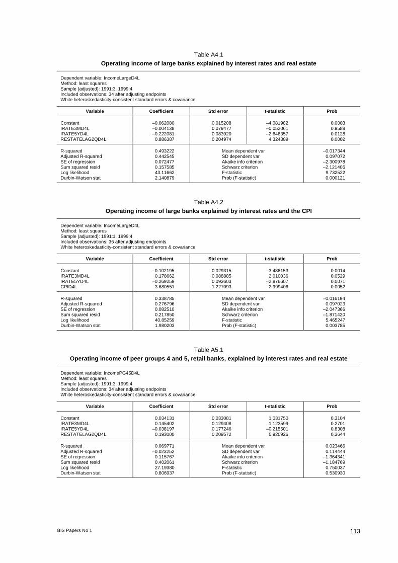
The development of operating income of large Austrian banks can be explained by a similar model tothat for the banking industry as a whole. Operating income of large banks depends significantlyand negatively on long-term interest rate developments and significantly and positively on realestate price developments in Vienna (lagged by two quarters). The difference compared to themodel for the banking industry as a whole is that short-term interest rates become totally insignificant

6 For practical reasons, real long-term interest rates are defined as the yield of five-year government benchmark bonds minusthe annual inflation rate in the corresponding quarter.

104 BIS Papers No 1

(see Table A4.1). Nevertheless, the explanatory power of this model remains high (adjusted R²: 0.44;Durbin-Watson test: 2.1). Viennese real estate prices become even more significant, which fits wellwith expectations. The largest Austrian banks are based in Vienna and are usually very active in theViennese real estate sector.

Substituting the CPI for real estate prices brings, to some extent, the same results: The operatingincome of large banks depends significantly and negatively on long-term interest ratedevelopments and significantly and positively on CPI developments (R²: 0.28; no autocorrelation;see Table A4.2). Short-term interest rate developments fall slightly short of being significant, ie remainslightly above the probability level of 5%, but, unlike the results so far, correlate positively withoperating income.

Using real interest rates instead of nominal rates and the CPI, the result is that falling real long-terminterest rates significantly lead to rising operating income, while rising real short-term rates havean insignificant effect on operating income.

Retail banks (peer group 4 and 5)

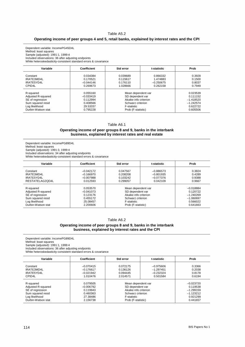
Applying the model with interest rates and real estate prices as the explanatory variables to “peergroups 4 and 5”, ie retail banks, does not explain operating income developments (see Table A5.1).Neither interest rate nor real estate price developments in Vienna have a significant influence on theoperating income of retail banks. This is not surprising, since small retail banks are mainly involved inthe customer deposits and lending business, which is in general, according to our analysis of netinterest income, not well explained by interest rate developments. The fact that real estate pricedevelopments in Vienna do not explain the operating income of small retail banks is reasonable. Smallretail banks are usually not based in Vienna and in general do not have significant real estateoperations in Vienna.

Substituting the CPI for real estate prices leads to very much the same results. Consumer pricedevelopments and - according to our interpretation of CPI developments during the 1990s - increasedcompetition appear to have no significant effect on the operating income of small retail banks (seeTable A5.2).

Banks specialising in interbank business

The operating income of - relatively small - banks operating mainly in the interbank area (peer group 8and 9) cannot be explained by interest rates and real estate prices. Changes in real estate pricesand long-term interest rates do not have any explanatory power; moreover, short-term interestrates are insignificantly (negatively) correlated with operating income. Inflation does notsignificantly explain the operating income of this banking sector, either (see Tables A6.1 and A6.2).

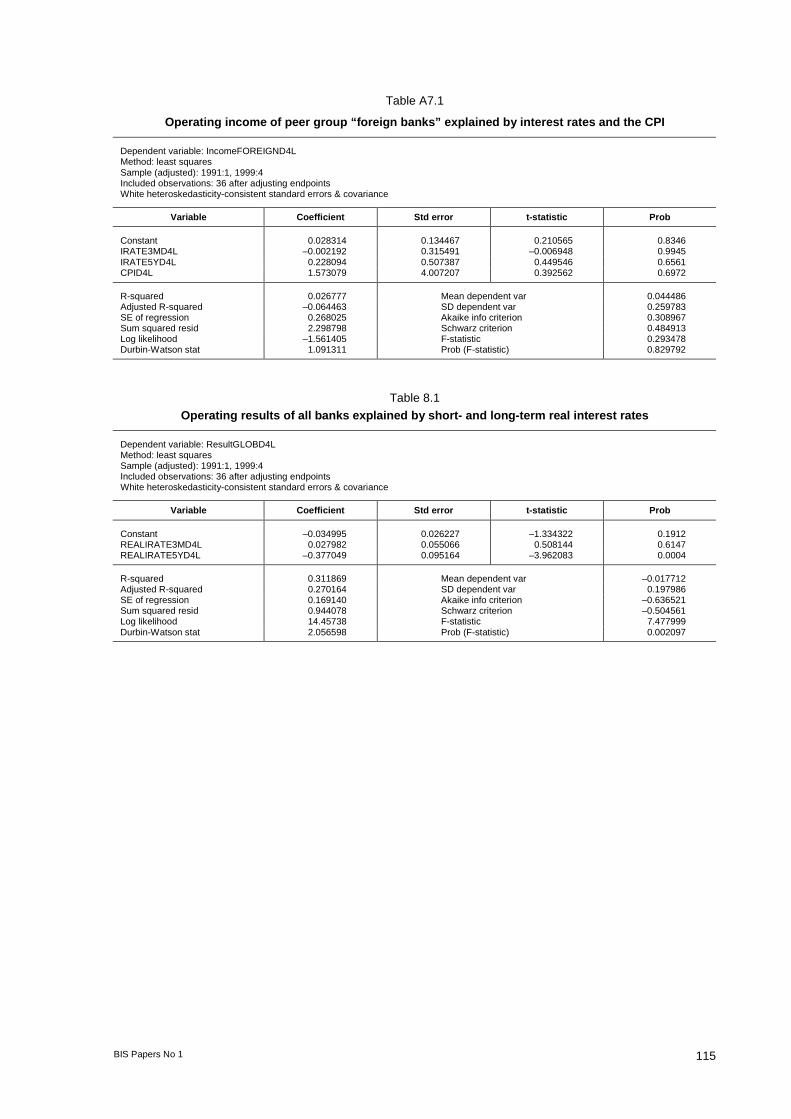
Foreign banks

Foreign banks’ operating income, ie the operating income of relatively small Austrian banks withsizeable operations abroad, does not have any significant regressions with real estatedevelopments in Vienna and with interest rates, which is by and large in line with expectations. CPIdevelopments in Austria have no significant effect on the operating income of small Austrian banksoperating abroad, either (see Table A7.1).

In conclusion, for the banking industry as a whole, developments in short-term interest rates andlong-term interest rates, along with real estate and/or the inflation rate, appear to have a significantinfluence on operating income. But this can be traced mainly to the behaviour of large banks, eventhough the influence of short-term interest rates on the operating income of large banks becomesinsignificant or difficult to interpret. Small retail banks, (smaller) foreign banks and (smaller) banks inthe interbank business seem to be unaffected not only by real estate price developments in Vienna(which is in line with expectations), but also by consumer prices and interest rate developments.

2.4 Real fundamentals, monetary aggregates and financial market dataReal GDP

In a simple regression model, real GDP growth rates correlate significantly negatively with theoperating income of both the Austrian banking sector as a whole and that of most peer groups, whichis contrary to expectations (see Table A3.2). However, in multiple regression models real GDP growthrates usually do not explain operating income significantly.

BIS Papers No 1 105

These results are even more astonishing, as we found strong seasonal patterns in operating income,similar to the ones for GDP; ie the first quarter - in absolute terms - is usually the weakest, and thefourth quarter usually the strongest of the year. The latter might have to do with the fact that bankstend to charge their annual service fees, interest due, etc at the end of the year, ie in the fourthquarter.

Real domestic demand

Real domestic demand growth as an explanatory variable for operating income of Austrian banksleads very much to the same results as for real GDP.

M3 and loans

We found some positive correlations between M3 growth or loan growth with operating income,which are usually not significant (apart from Table A3.3). The positive relationship is in line withexpectations, since growing monetary aggregates should lead to higher income volumes and probablyhigher margins.

Stock markets

Stock market developments seem to have no significant explanatory power for the operatingincome of Austrian banks.7 This is in line with expectations, since stocks play only a minor role in theAustrian economy. Austrian investors and Austrian banks are not known to be - relative to their size -big players on stock markets (with the exception of eastern European stock markets).

Yield curve

Apart from using short- and long-term interest rates, we also tested how the dynamics of the yieldcurve might explain operating income. In general, no convincing regressions were found.

2.5 Banks’ operating result and macroeconomic developmentsThe operating result is operating income minus operating expenses. Operating expenses aremainly influenced by microeconomic-related costs. Given this definition of the operating result, onemight expect models similar to those which explain the operating income to also explain, to someextent, the operating result of Austrian banks.

Short-, long-term interest rates and real estate prices

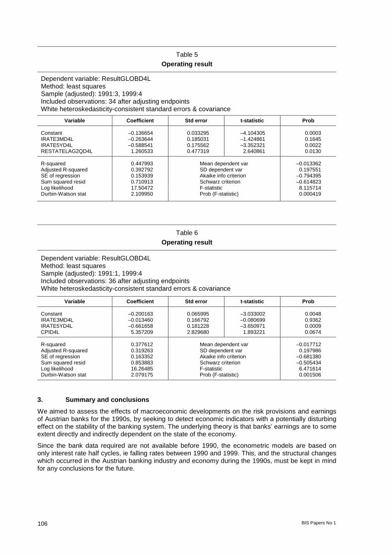
First, we explain the operating result of the global Austrian banking industry by short- and long-terminterest rates, as well as by the Viennese real estate price index lagged by two quarters; see Table 5.The results are largely in line with those achieved with the model for operating income. Falling long-term interest rates and rising real estate prices lagged by two quarters significantly lead to arising operating result, while short-term interest rates insignificantly explain the operating result.

Short-, long-term interest rates and the consumer price index

Substituting the consumer price index for the real estate price index decreases the explanatory valueof the model somewhat; see Table 6. Long-term interest rates are highly significant, and the CPIfalls slightly short of being significant in explaining the operating result, while short-term interestrates are totally insignificant. Falling long-term interest rates lead to a higher operating result.

Real short- and long-term interest rates

Using real short- and long-term interest rates instead of nominal interest rates and the CPI leads to thefollowing result: real long-term interest rates have a significant negative correlation with theoperating result, while real short-term interest rates have no explanatory power (see Table A8.1).

From the above results, we draw the conclusion that short-term interest rates, or monetary policy,had a minor influence on bank’s operating results during the 1990s.

7 We used the Austrian Traded Index (ATX) and Datastream’s EU Market Index.

106 BIS Papers No 1

Table 5Operating result

Dependent variable: ResultGLOBD4LMethod: least squaresSample (adjusted): 1991:3, 1999:4Included observations: 34 after adjusting endpointsWhite heteroskedasticity-consistent standard errors & covariance




Table 6Operating result



Constant –0.200163 0.065995 –3.033002 0.0048IRATE3MD4L –0.013460 0.166792 –0.080699 0.9362IRATE5YD4L –0.661658 0.181228 –3.650971 0.0009CPID4L 5.357209 2.829680 1.893221 0.0674


3. Summary and conclusionsWe aimed to assess the effects of macroeconomic developments on the risk provisions and earningsof Austrian banks for the 1990s, by seeking to detect economic indicators with a potentially disturbingeffect on the stability of the banking system. The underlying theory is that banks’ earnings are to someextent directly and indirectly dependent on the state of the economy.

Since the bank data required are not available before 1990, the econometric models are based ononly interest rate half cycles, ie falling rates between 1990 and 1999. This, and the structural changeswhich occurred in the Austrian banking industry and economy during the 1990s, must be kept in mindfor any conclusions for the future.

BIS Papers No 1 107

The main findingsRisk provisions

We found evidence that Austrian banks behave procyclically, ie banks increase their risk provisionsin times of declining real GDP growth rates. They also raise their risk provisions when theiroperating income increases. It cannot be ruled out that banks form risk provisions because theiroperating result rises, with the aim of smoothing their operating results over time, perhaps due tocredibility and/or tax considerations.

That banks should increase their risk provisioning in times of rising operating income is in the interestof supervisors, because higher return or income goes with higher risks, for which risk provisionsshould be expanded accordingly. However, if banks increase their risk provisions because of a risingoperating result, several questions arise. Is this behaviour triggered by the aim of evening out theoperating result (and thereby profits) over time, in order to generate trust among the public? has itsomething to do with tax considerations? or do some individual banks increase risk provisions simplywhen they can afford to do so?

The model also delivers the unexpected and somewhat curious result that rising real estate prices leadto higher risk provisions. Generally in line with expectations is the result that falling inflation depressesrisk provisions.

Net interest income

Net interest income appears to be uncorrelated with real GDP growth. Difficult to interpret is thebehaviour of net interest income in relation to short- and long-term interest rate developments. Itappears that net interest income is by and large uncorrelated with interest rate developments, eventhough we cannot yet rule out that net interest income reacts to interest rate developments with verylong time lags of perhaps up to four years.

However, we believe that very low interest rate levels lead to declining net interest income. Atvery low interest rate levels, interest rates for retail deposits reach a point where they cannot fall muchfurther (eg in the case of overnight deposits), and/or customers start to move to other, higher-yieldforms of investment (eg mutual funds), while interest rates on loans still have room left to decline andbecome even more attractive for debtors.

Bank operating income

When it comes to explaining the development of the operating income of the Austrian bankingindustry as a whole, short- and long-term interest rates as well as real estate and/or inflation have asignificant influence. Falling interest rates and rising real estate prices, as well as rising inflation,lead to higher operating income and vice versa.

In an environment of falling interest rates, operating income rises and vice versa. This type ofbehaviour is in line with expectations. Banks in general appear to refinance themselves short-term,while they invest long-term (this holds not only for investment banking, but also for investments ineg equipment, real estate and human capital).

Rising real estate prices have a positive impact on the operating income of banks, since their ownreal estate transactions and those of their real estate subsidiaries become more profitable. In addition,rising real estate prices should lead to higher demand for mortgage-backed debt, which in turnincreases the volume of commissions, fees, etc and probably margins.

In relation to bank operating income, the consumer price index might well be used as an indicator forstructural changes and especially for competition during the 1990s in Austria. High inflation or risinginflation rates could - amongst other things - be an indicator for inefficiency and protected orfragmented markets. Low inflation or falling inflation rates could be associated with increasedcompetition. The latter is very much in line with developments in Austria during the 1990s, especiallyafter accession to the European Economic Area, and shortly afterwards to the European Union in1995.

When the Austrian banking sector is broken down into peer groups, the individual peer groupresults deviate from the overall conclusion: The influence of real estate and the CPI on the operatingincome of the whole banking sector can be traced solely to large banks. (Small) retail banks, (small)foreign banks and (small) banks specialising in interbank business appear to be unaffected not only bythe CPI and real estate price developments in Vienna, but also by short- and long-term interest ratedevelopments. Along with the inflation rate and/or retail prices, long-term interest rates appear to be

108 BIS Papers No 1

significant for the development of the operating income of large banks, which represent nearly threequarters of all Austrian banks in terms of total assets. The influence of short-term interest rates on theoperating income of large banks becomes insignificant or difficult to interpret.

Depending on the model specification, real GDP growth appears to have no significant explanatoryvalue for the income development of the Austrian banking sector. This result is somewhat astonishing,as we have found strong seasonal patterns in operating income, similar to the ones for GDP ordomestic demand; ie the first quarter is - in absolute terms - the weakest, the fourth quarter usually thestrongest.

Bank operating result

By and large, similar conclusions to those for bank operating income can be drawn for thedevelopment of the operating result of Austrian banks. In particular, declining real estate, but alsodeclining inflation, ie rising competition in Austria during the 1990s, appears to have a negative impacton the operating result of Austrian banks. However, short-term interest rates seem to have nosignificant influence on banks’ operating results.

Real long-term interest rates have a significant negative correlation with the operating result, realshort-term interest rate are completely insignificant.

The fact that short-term interest rates had no significant influence on banks’ operating results duringthe 1990s leads us to the conclusion that monetary policy appears to have played a minor role inexplaining the operating result of the Austrian banking industry.

Possible implications for banking supervision and some general, tentative conclusions

Austrian banks seem to behave procyclically, ie they increase risk provisions in times of decliningreal GDP growth rates. In addition, they form risk provisions when operating income rises. It cannot beruled out that banks form risk provisions because their operating result rises. From a supervisor’s pointof view, a less procyclical stance, ie the forming of risk provisions in economic “good times” (rising orhigh real GDP growth rates), should be encouraged; the expected loan losses should includeexpected losses due to the business cycle. From a European perspective, further harmonisationefforts in the area of accounting standards, provisioning and taxation should possibly be envisaged toachieve a level playing field.

Overall, some macroeconomic variables like interest rates, real estate and consumer prices, but notreal GDP or domestic demand growth rates, can be used to explain the risk provisions, operatingincome and operating results of Austrian banks during the 1990s.8 Consequently, the macroeconomicdimension must not be neglected by supervisory authorities. However, macroeconomic developmentsalone cannot explain the development of microeconomic bank data in a sufficient way. Other factorsapart from macroeconomics obviously play a major role in banking.

Microeconomics, especially sound and prudent bank management - at least during normal (bank)business cycles - probably plays the major role for individual banks. For supervisors, the “bottomup” approach, ie standard banking supervision, remains most relevant.

Structural changes, such as increased competition, accession to the single market and the openingup of eastern European markets, have certainly also been influencing Austrian banks strongly andmust be monitored by market participants and the relevant authorities.

8 However, we regard it as likely that more pronounced business cycles than Austria has experienced during the 1990s mighthave an impact on bank data.

BIS Papers No 1 109

Appendix

Table A1.1Risk provisions (of all Austrian banks) explained by real GDP growth, the real estate price index lagged

by two quarters, the real three-month interest rate and a dummy variable (D96)



Constant 0.063477 0.021137 3.003051 0.0055GDPREALD4L –2.680895 0.907689 –2.953540 0.0062RESTATELAG2QD4L 1.194800 0.155739 7.671790 0.0000REALIRATE3MD4L –0.098680 0.024024 –4.107562 0.0003D96 –0.369404 0.012471 –29.62151 0.0000


Table A1.2Risk provisions explained by an AR model (lag four quarters) using realGDP, real estate lagged by two quarters, the CPI and a dummy variable

Dependent variable: ProvisionsGlobalD4LMethod: least squaresSample (adjusted): 1992:3, 1999:4Included observations: 30 after adjusting endpointsConvergence achieved after 11 iterationsWhite heteroskedasticity-consistent standard errors & covariance


Constant –0.017004 0.026877 –0.632658 0.5329GDPREALD4L –3.077624 0.990161 –3.108205 0.0048RESTATELAG2QD4L 0.605490 0.162714 3.721204 0.0011CPID4L 5.019448 0.742043 6.764364 0.0000D96 –0.357067 0.014583 –24.48497 0.0000AR(4) –0.577672 0.156050 –3.701843 0.0011


Table A1.3Risk provisions explained by operating income and a dummy variable



Constant 0.078750 0.014963 5.262981 0.0000IncomeGLOBD4L 1.006263 0.200560 5.017257 0.0000D96 –0.425653 0.043801 –9.717924 0.0000


110 BIS Papers No 1

Table A1.4Risk provisions explained by operating result and a dummy variable



Constant 0.067594 0.016941 3.989960 0.0003ResultGLOBD4L 0.264865 0.081501 3.249841 0.0027D96 –0.423443 0.050626 –8.364081 0.0000


Table A1.5Risk provisions explained by an AR model (lag four quarters) using operating results,

real GDP, real estate lagged by two quarters, the CPI and a dummy variable

Dependent variable: ProvisionsGlobalD4LMethod: least squaresSample (adjusted): 1992:3, 1999:4Included observations: 30 after adjusting endpointsConvergence achieved after 14 iterationsWhite heteroskedasticity-consistent standard errors & covariance


Constant –0.010389 0.026717 –0.388865 0.7010IncomeGLOBD4L 0.372042 0.152837 2.434233 0.0231BIPREALD4L –2.150079 0.916814 –2.345164 0.0280RESTATELAG2QD4L 0.537019 0.144434 3.718088 0.0011CPID4L 4.229359 0.862626 4.902887 0.0001D96 –0.365138 0.014292 –25.54842 0.0000AR(4) –0.451055 0.151922 –2.968994 0.0069


Table A2.1Operating income of all Austrian banks explained by net interest income

Dependent variable: IncomeGlobalD4LMethod: least squaresSample (adjusted): 1991:1, 1999:4Included observations: 36 after adjusting endpointsWhite heteroskedasticity-consistent standard errors & covariance


Constant 0.005177 0.009619 0.538202 0.5939NetInterestIncomeD4L 0.749191 0.130168 5.755593 0.0000


BIS Papers No 1 111

Table A2.2Net interest income of all banks explained by real GDP growth and short- and long-term interest rates

Dependent variable: NetInterestIncomeD4LMethod: least squaresDate: 30 November 2000 Time: 15:40Sample (adjusted): 1991:1, 1999:4Included observations: 36 after adjusting endpointsWhite heteroskedasticity-consistent standard errors & covariance


Constant –0.014571 0.031056 –0.469173 0.6421BIPREALD4L –1.097277 1.200252 –0.914206 0.3674IRATE3MD4L –0.100834 0.067323 –1.497765 0.1440IRATE5YD4L 0.040665 0.072035 0.564519 0.5763


Table A3.1Operating income of all Austrian banks explained by short- and long-term interest rates

Dependent variable: IncomeGlobalD4LMethod: least squaresDate: 24 November 2000 Time: 14:58Included observations: 36 after adjusting endpointsWhite heteroskedasticity-consistent standard errors & covariance


Constant –0.035499 0.011167 –3.179029 0.0032IRATE3MD4L –0.065340 0.052391 –1.247140 0.2211IRATE5YD4L –0.136139 0.068295 –1.993385 0.0545


Table A3.2Operating income of all banks explained by real GDP growth

Dependent variable: IncomeGLOBD4LMethod: least squaresSample (adjusted): 1991:1, 1999:4Included observations: 36 after adjusting endpointsWhite heteroskedasticity-consistent standard errors & covariance


Constant 0.034065 0.029198 1.166699 0.2515BIPREALD4L –2.493492 1.140224 –2.186844 0.0357


112 BIS Papers No 1

Table A3.3

Operating income of all banks explained by loan growth and short- and long-term interest rates

Dependent variable:Method: least squaresSample (adjusted): 1991:1, 1999:4Included observations: 36 after adjusting endpointsWhite heteroskedasticity-consistent standard errors & covariance


Constant –0.094401 0.027634 –3.416156 0.0017IRATE3MD4L –0.092329 0.050389 –1.832336 0.0762IRATE5YD4L –0.141305 0.065733 –2.149682 0.0392DIRECTLOANSD4L 1.060479 0.541573 1.958145 0.0590


Table A3.4Operating income of all banks explained by short- and long-term interest rates and the inflation rate (CPI)

Dependent variable: IncomeGlobalBD4LMethod: least squaresSample (adjusted): 1991:1, 1999:4Included observations: 36 after adjusting endpointsWhite heteroskedasticity-consistent standard errors & covariance




Table A3.5Operating income of all banks explained by real short- and long-term interest rates

Dependent variable: ERTRAGGLOBD4LMethod: least squaresSample (adjusted): 1991:1, 1999:4Included observations: 36 after adjusting endpointsWhite heteroskedasticity-consistent standard errors & covariance


Constant –0.023019 0.009359 –2.459532 –2.459532REALIRATE3MD4L –0.026220 0.020029 –1.309118 –1.309118REALIRATE5YD4L –0.095183 0.039199 –2.428205 –2.428205


BIS Papers No 1 113

Table A4.1Operating income of large banks explained by interest rates and real estate

Dependent variable: IncomeLargeD4LMethod: least squaresSample (adjusted): 1991:3, 1999:4Included observations: 34 after adjusting endpointsWhite heteroskedasticity-consistent standard errors & covariance




Table A4.2Operating income of large banks explained by interest rates and the CPI

Dependent variable: IncomeLargeD4LMethod: least squaresSample (adjusted): 1991:1, 1999:4Included observations: 36 after adjusting endpointsWhite heteroskedasticity-consistent standard errors & covariance


Constant –0.102195 0.029315 –3.486153 0.0014IRATE3MD4L 0.178662 0.088885 2.010036 0.0529IRATE5YD4L –0.269259 0.093603 –2.876607 0.0071CPID4L 3.680551 1.227093 2.999406 0.0052


Table A5.1Operating income of peer groups 4 and 5, retail banks, explained by interest rates and real estate

Dependent variable: IncomePG45D4LMethod: least squaresSample (adjusted): 1991:3, 1999:4Included observations: 34 after adjusting endpointsWhite heteroskedasticity-consistent standard errors & covariance


Constant 0.034131 0.033081 1.031750 0.3104IRATE3MD4L 0.145402 0.129408 1.123599 0.2701IRATE5YD4L –0.038197 0.177246 –0.215501 0.8308RESTATELAG2QD4L 0.193000 0.209572 0.920926 0.3644

R-squared 0.069771 Mean dependent var 0.023466Adjusted R-squared –0.023252 SD dependent var 0.114444SE of regression 0.115767 Akaike info criterion –1.364341Sum squared resid 0.402061 Schwarz criterion –1.184769Log likelihood 27.19380 F-statistic 0.750037Durbin-Watson stat 0.806937 Prob (F-statistic) 0.530930

114 BIS Papers No 1

Table A5.2Operating income of peer groups 4 and 5, retail banks, explained by interest rates and the CPI



Constant 0.034384 0.039689 0.866332 0.3928IRATE3MD4L 0.170521 0.115617 1.474883 0.1500IRATE5YD4L –0.044146 0.176110 –0.250675 0.8037CPID4L 0.269673 1.028666 0.262158 0.7949

R-squared 0.055160 Mean dependent var 0.023539Adjusted R-squared –0.033419 SD dependent var 0.111152SE of regression 0.112994 Akaike info criterion –1.418520Sum squared resid 0.408566 Schwarz criterion –1.242574Log likelihood 29.53337 F-statistic 0.622722Durbin-Watson stat 0.795228 Prob (F-statistic) 0.605506

Table A6.1Operating income of peer groups 8 and 9, banks in the interbank

business, explained by interest rates and real estate




R-squared 0.053570 Mean dependent var –0.018884Adjusted R-squared –0.041073 SD dependent var 0.120722SE of regression 0.123176 Akaike info criterion –1.240269Sum squared resid 0.455172 Schwarz criterion –1.060697Log likelihood 25.08457 F-statistic 0.566022Durbin-Watson stat 2.200606 Prob (F-statistic) 0.641663

Table A6.2Operating income of peer groups 8 and 9, banks in the interbank

business, explained by interest rates and the CPI




R-squared 0.079505 Mean dependent var –0.023720Adjusted R-squared –0.006792 SD dependent var 0.119538SE of regression 0.119943 Akaike info criterion –1.299159Sum squared resid 0.460363 Schwarz criterion –1.123212Log likelihood 27.38486 F-statistic 0.921299Durbin-Watson stat 2.156738 Prob (F-statistic) 0.441657

BIS Papers No 1 115

Table A7.1

Operating income of peer group “foreign banks” explained by interest rates and the CPI

Dependent variable: IncomeFOREIGND4LMethod: least squaresSample (adjusted): 1991:1, 1999:4Included observations: 36 after adjusting endpointsWhite heteroskedasticity-consistent standard errors & covariance


Constant 0.028314 0.134467 0.210565 0.8346IRATE3MD4L –0.002192 0.315491 –0.006948 0.9945IRATE5YD4L 0.228094 0.507387 0.449546 0.6561CPID4L 1.573079 4.007207 0.392562 0.6972

R-squared 0.026777 Mean dependent var 0.044486Adjusted R-squared –0.064463 SD dependent var 0.259783SE of regression 0.268025 Akaike info criterion 0.308967Sum squared resid 2.298798 Schwarz criterion 0.484913Log likelihood –1.561405 F-statistic 0.293478Durbin-Watson stat 1.091311 Prob (F-statistic) 0.829792

Table 8.1Operating results of all banks explained by short- and long-term real interest rates



Constant –0.034995 0.026227 –1.334322 0.1912REALIRATE3MD4L 0.027982 0.055066 0.508144 0.6147REALIRATE5YD4L –0.377049 0.095164 –3.962083 0.0004


116 BIS Papers No 1

References

Blejer, M I, E V Feldman and A Feltenstein (1997): “Exogenous Shocks, Deposit Runs and BankSoundness: A Macroeconomic Framework”, IMF Working Paper, 97/91.

Caprio, G and D Klingebiel (1996): “Bank Insolvency, Bad Luck, Bad Policy or Bad Banking?”, AnnualWorld Bank Conference on Development 1996, IBRD, Washington DC.

Crockett, A (1997): “The Theory and Practice of Financial Stability”, Essays in International Finance,Princeton University.

Davis, E P (1995a): “Debt, Financial Fragility and Systemic Risk (revised and extended version)”,Oxford University Press.

Davis, E P (1995b): “Financial Fragility in the Early 1990s. What can be Learnt from InternationalExperience?”, LSE Financial Markets Group Special Paper No 76.

Demirguc-Kunt, A and E Detragiache (1998): “The Determinants of Banking Crises in Developing andDeveloped countries”, IMF Staff Papers, 45, pp 81-109.

Gavin and Hausman (1995): “The Roots of Banking Crises. The Macroeconomic Context”,Washington DC.

Gonzáles-Hermosillo, B (1999): “Determinants of Ex-Ante Banking System Distress: A Macro-MicroEmpirical Exploration of Some Recent Episodes”, IMF Working Paper, 99/33.

Gorton, G (1988): “Banking Panics and Business Cycles”, Oxford Economic Papers, 40, pp 751-81.

Hardy, D C and C Pazarbasioglu (1998): “Leading Indicators of Banking Crises. Was Asia different?”,IMF Working Paper, 98/91.

IMF (1999): “Macro-Prudential Indicators and Data Dissemination”, IMF Consultative Document,September 1999.

Kaminsky, G L (1999): “Currency and Banking Crises: The Early Warning of Distress”, Paperpresented at the IMF Institute course on “An Early Warning System for Financial Crises”, May 1999.

Lindgren, C J, G Garcia and M I Saal (1996): “Bank Soundness and Macroeconomic Policy”, IMF,Washington DC.

Mishkin, F S (1994): “Preventing Financial Crises. An International Perspective”, NBER WorkingPaper, 4636.

OECD (1992): “Banks Under Stress”, Paris.

Peek, J, E S Rosengreen and G M B Tootell (1999): “Using Bank Supervisory Data to ImproveMacroeconomic Forecasts”, New England Economic Review, Federal Reserve Bank of BostonSep/Oct 1999, pp 21-32.

Sharma, S (1999): “The Challenge of Predicting Economic Crises”, Finance & Development, June1999, pp 40-42.

Turner, J (1999): “The Austrian Supervisory Risk Assessment System”, in Focus on Austria 1/2000,Oesterreichische Nationalbank, pp 50-60.

Vihriälä, V (1997): “Banks and the Finnish Credit Cycle 1986-1995”, Bank of Finland Studies E:7.

Documents

The influence of macroeconomic developments on Austrian banks