3

The industrial-organization approach to international trade ("new trade theory") has

incorporated features of increasing returns to scale, imperfect competition, and product

differentiation into traditional general-equilibrium trade models. These new models offer rich

predictions about the direction and volume of trade between two countries as functions of

industry characteristics (factor intensities, scale economies, product differentiation) interacting

with country characteristics (relative size differences, relative endowment differences, and trade

costs).

However, an awkward empirical problem is that most of the firms and industries

motivated by the IO approach to trade are multinational firms, while most of the theory has been

about single-plant national firms. More recent theoretical developments have incorporated

multinational firms, which maintain facilities in more than one country. These multinationals are

often broken down into "horizontal" firms, which produce the same goods and services in multiple

countries, and "vertical" firms, which geographically fragment production by stages. An early

example of a model with vertical multinationals is in Helpman (1984) while an early model of

horizontal multinationals is in Markusen (1984).

Subsequent theoretical work has focused on horizontal firms because they seem to be

more prevalent in the world. Examples include Horstmann and Markusen (1987, 1992), Brainard

(1993a), and Markusen and Venables (1996, 1997, 1998). These models have since been

subjected to empirical tests, especially by Brainard (1993b, 1997) and Ekholm (1995, 1997a,b,

1998). Results give good support to the theoretical predictions of the "horizontal" models:

multinational activity should be concentrated among countries that are relatively similar in both

size and in relative endowments (or per capita incomes).

4

Theoretical models combining both horizontal and vertical motives for direct investment

are analytically difficult. Helpman's original model of vertical multinationals relied on the

assumption of no trade costs, but in that case there is no motive for horizontal multinationals

(given plant-level scale economies). For analytical tractability, the early models of horizontal

firms assumed that different activities (e.g., headquarters services and plant production) use

factors in the same proportion or that there is only one factor of production. However, this

permits no factor-price motive for vertical fragmentation across countries.

Two recent models exist in which both vertical and horizontal firms can arise

endogenously due to the simultaneous existence of trade costs and different factor intensities

across industries. Analytical difficulties, however, imply that most results are derived from

numerical simulations (Markusen (1997), Markusen, et al (1996)). These simulations generate a

number of testable implications, relating direct investment to country characteristics.

The purpose of this paper is therefore to take the theoretical predictions of recent theory

and subject them to econometric test. We begin by reviewing this newer theory and discussing its

theoretical predictions. The theory explains the volume of production of foreign affiliates of one

country’s firms in another country as a function of the characteristics of both countries. For

example, production by affiliates of the parent-country firms in the host country will be high if the

countries are similar in size and trade costs are high, in which case affiliates are horizontal.

Production will also be high if the parent country is small and skilled-labor abundant relative to

the host nation and trade costs are low, in which case affiliates are vertical.

Next we translate these predictions into a tractable empirical specification. The theory

predicts that many relationships are interactive or non-linear. For one example, an increase in

5

trade costs will increase production by affiliates if the countries are similar (direct investment is

horizontal) but may decrease investment if the countries are different in relative endowments

(direct investment is vertical). For another, the effect of an increase in the parent country’s GNP

level on production by affiliates of its firms abroad is non-monotonic. It increases if the parent

country is small but decreases if the size of the parent country exceeds the size of the host

country. Further, the effect of an increase in the parent country relative endowment of skilled

labor on production by its firms’ affiliates are positive and large if trade costs are small (vertical

investment is encouraged) but are smaller if trade costs are large. Finally, the volume of affiliate

production is highest when the parent country is both skilled-labor abundant and small relative to

the host country.

Results of our estimations are closely consistent with the theory. The volume of affiliate

sales follows the theoretical predictions based on characteristics of both parent and host countries.

Both vertical and horizontal investments are important and related to country characteristics as

the model predicts.

2. The Theoretical Model

We now present a theoretical model drawn from Markusen (1997) and Markusen,

Venables, Konan and Zhang (1996). First, we present a broad outline of the model, and then

discuss crucial assumptions about the level and composition of fixed costs. The model assumes

the existence of two homogeneous goods (X and Y), two countries (h and f), and two

homogeneous factors, unskilled labor (L) and skilled labor (S), which are internationally

immobile. Good Y is labor-intensive and produced under constant returns to scale in a

6

competitive industry. Good X is skilled-labor-intensive overall, exhibits increasing returns to

scale, and is subject to Cournot competition with free entry and exit. In this good headquarters

services and plant facilities may be geographically separated and a firm may have plants in one or

both countries.

With this structure, there are six firm types, with free entry and exit into and out of firm

types. Regime denotes a set of firm types active in equilibrium. Firm types are as follows:

Type mh - horizontal multinationals that maintain plants in both countries with

headquarters located in country h.

Type mf - horizontal multinationals that maintain plants in both countries with

headquarters located in country f.

Type nh - national firms that maintain a single plant and headquarters in country h;

they may or may not export to country f.

Type nf - national firms that maintain a single plant and headquarters in country f;

they may or may not export to country h.

Type vh - vertical multinationals that maintain a single plant in country f and

headquarters in country h; they may or may not export to country h.

Type vf - vertical multinationals that maintain a single plant in country h and

headquarters in country f; they may or may not export to country f.

In the model, national markets for goods are segmented and transport costs use unskilled

labor. Type-v firms incur a small cost penalty relative to type-n firms as a "transactions cost" of

geographically separating plant and headquarters.

Assumptions about the size and composition of fixed costs are crucial to the predictions of

7

the model.1 First, we assume the existence of multi-plant economies of scale (relevant to type-m

firms) due to a joint-input property of knowledge capital. Headquarters service (blueprints,

manuals, formulas, procedures, etc.) can be supplied to additional plants at low marginal cost.

Thus, in good X the total fixed costs of headquarters and two plants is less than the double the

total fixed costs of a single-plant firm (the joint-input property of knowledge capital).

Second, it is assumed that headquarters services are more skilled-labor-intensive than

production. Somewhat more controversial is our assumption that plant-level production is more

skilled-labor-intensive than the composite rest of the economy. Thus, we stipulate that the

ranking of skilled-labor intensity of activities is [headquarters only] > [integrated X] > [plant

only] > [Y].

Finally, we assume that two-plant type-m firms are more skilled-labor-intensive than either

type-n or type-v firms. The hypothesis is that type-m firms use additional skilled labor both at

home and in the host country in managing and operating the second plant. Type-n and type-v

firms use additional unskilled labor in transport costs in serving the foreign market.2 Thus, the

skilled-labor- intensity ranking of firm types is [type-m firms] > [type-v and type-n firms] .

The full set of equations and inequalities characterizing equilibrium in the model is given in

Markusen (1997) and in Markusen, et al (1996) and we will not repeat that exercise here. In the

next section, we link the assumptions about technology to country characteristics in order to

1 The following assumptions draw empirical support from a large number of studies, including Aitken et al(1995), Blomstrom et al (1997), Caves (1996), Ekholm (1995, 1997a, 1997b), Feenstra and Hanson (1997), Lipseyet al (1995), Slaughter (1999), and UNCTAD (1993). Data drawn from some of these sources are presented inMarkusen (1997).

2 This particular assumption does not play a significant role in this paper but does lead to interesting factor-marketeffects from investment liberalization, such as the relative wage of skilled labor can rise in both countries(Markusen, 1997).

8

generate predictions about multinational actively as a function of those country characteristics.

3. Active Firm Types and Country Characteristics

We explain country characteristics that favor various firm types producing or maintaining

headquarters in country h. Analogous comments apply to firms in country f. Consider first

factors that favor national firms headquartered in country H and also producing there.

Assumptions of the model developed above suggest that type nh firms will be the dominant type

active in h if: (1) h is both large and skilled-labor abundant; (2) h and f are similar in size and

relative endowments and transport costs are low (type nf will sell in h); or (3) foreign investment

barriers in f are high (type nf may sell in h).3

Country h being large supports production there while skilled-labor abundance favors

locating headquarters in h as well. Thus, an integrated type-nh firm has a cost advantage over a

type-vh or vf firm. A type-nh firm also has an advantage over a type-mh firm, which must locate

costly capacity in the small f market unless trade costs are high. Type-n firms should also be

dominant when the countries are similar and trade costs are small. If countries are perfectly

symmetric, for example, there is no motive for type-v firms given the assumption of a small cost

penalty to separating activities. Small trade costs favor type-n firms over two-plant type-m firms.

Type-mh firms will be the dominant type active in country h if the nations are similar in

size and relative endowments and transport costs are high (type mf will also produce in h). Thus,

horizontal multinationals firms should be associated with similarities between countries in both

size and in relative factor endowments. The intuition behind is that if countries are dissimilar in

3 The word “dominant” means that the number of firms of this type is larger than the number of firms of any other

9

either size or relative endowments, one country will be "favored" as a site of production and/or

headquarters. For example, if the countries are similar in relative endowments but of different

sizes, then national firms located in the large country will be favored because they avoid costly

capacity in the smaller market. If the countries are different in relative endowments but of similar

size, then there is an incentive to concentrate headquarters in the skilled-labor-abundant country

and production in the skilled-labor-scarce country. Thus vertical firms headquartered in the

skilled-labor-abundant countries are favored unless trade costs are high.

From this analysis two predictions about vertical multinationals follow directly. First,

type-vh firms will be dominant in h if country h is small, skilled-labor abundant, and transport

costs are not excessive. Second, type-vf firms will be dominant in h if country h is large, skilled-

labor scarce, and transport costs are not excessive.

4. Simulation Results

Data exist on the volume of production in host countries by affiliates of firms in parent

countries, but not on the number of firms of various types. Accordingly, we need to develop

predictions about affiliate production, rather than the numbers of firms of various types. In this

section, we solve the model numerically in order to generate such predictions on the relationship

between affiliate sales and country characteristics.4

A preliminary issue is to define "affiliate production" in the model in a way that relates

type in the associated equilibrium.4 The full model, consisting of 41 non-linear inequalities, is solved as a complementarity problem usingRutherford’s (1995) solver MPS/GE, a subsystem of GAMS. See Markusen (1997) and Markusen, et al (1996) for

10

sensibly to data on affiliate sales. Parents and affiliates in the data are essentially defined in terms

of ownership location. Thus, in our model we assume that the country in which a firm's

headquarters are located is the parent country. Given that assumption, the production of affiliates

of country-h firms in country f is the output of plants in country f "owned" by type-mh and type-vh

firms. Similarly, the volume of production by country-h affiliates of country f firms is the

production in country-h plants owned by type-mf and type-vf firms.

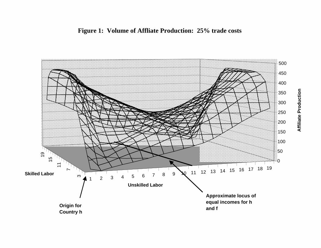
Simulation results are demonstrated with a series of world Edgeworth box diagrams in

Figures 1-5, with the total world endowment of skilled labor on the "Y" axis and the total world

endowment of unskilled labor on the "X" axis. The origin for country h is at the southwest (SW)

corner of the box and the origin for country f is at the northeast (NE) corner. Along the SW-NE

diagonal, the countries have identical relative endowments but differ in size. The locus along

which the countries have equal incomes but differ in relative endowments is steeper than the

diagonal and is not quite linear. The approximate locus along which the countries have equal

incomes is given by the line drawn on the floor of the box in Figure 1. Country h is smaller than

country f to the left of this locus and is larger to the right.

Figure 1 shows simulation outcomes at high trade costs, with affiliate production being the

sum of the outputs of both countries' affiliated plants. Note that Figure 1 contains a classic

saddle. Affiliate sales are at a minimum when the two countries are similar in relative

endowments but different in size, in which case national firms headquartered in the large country

dominate X production. Moving along the SW-NE diagonal (relative endowments identical),

total affiliate sales reach a maximum at the mid-point where the countries are identical. At this

the full set of equations and inequalities.

11

point, all firms are type-m and exactly half of all world production of X is affiliate production.

The other half is output of the domestic plants of type-m firms.

A somewhat surprising result in Figure 1 is that total affiliate production is highest when

one country is both small (but not too small!) and skilled-labor abundant. In such a situation,

type-v firms located in that country are the dominant firm-type. Note that if only type-v firms

were active in equilibrium, then all of the world production of X is affiliate sales. Conversely,

affiliate activity is lowest when the skilled-labor-abundant country is large, in which case all

production of X is by national firms headquartered in that country.

The non-linearities in Figure 1 present a challenge for testing. For example, the effect of

differences in country size on affiliate sales depends on whether the countries are similar in

relative endowments and, if they are different in size, on whether the small country is the skilled-

labor abundant country.

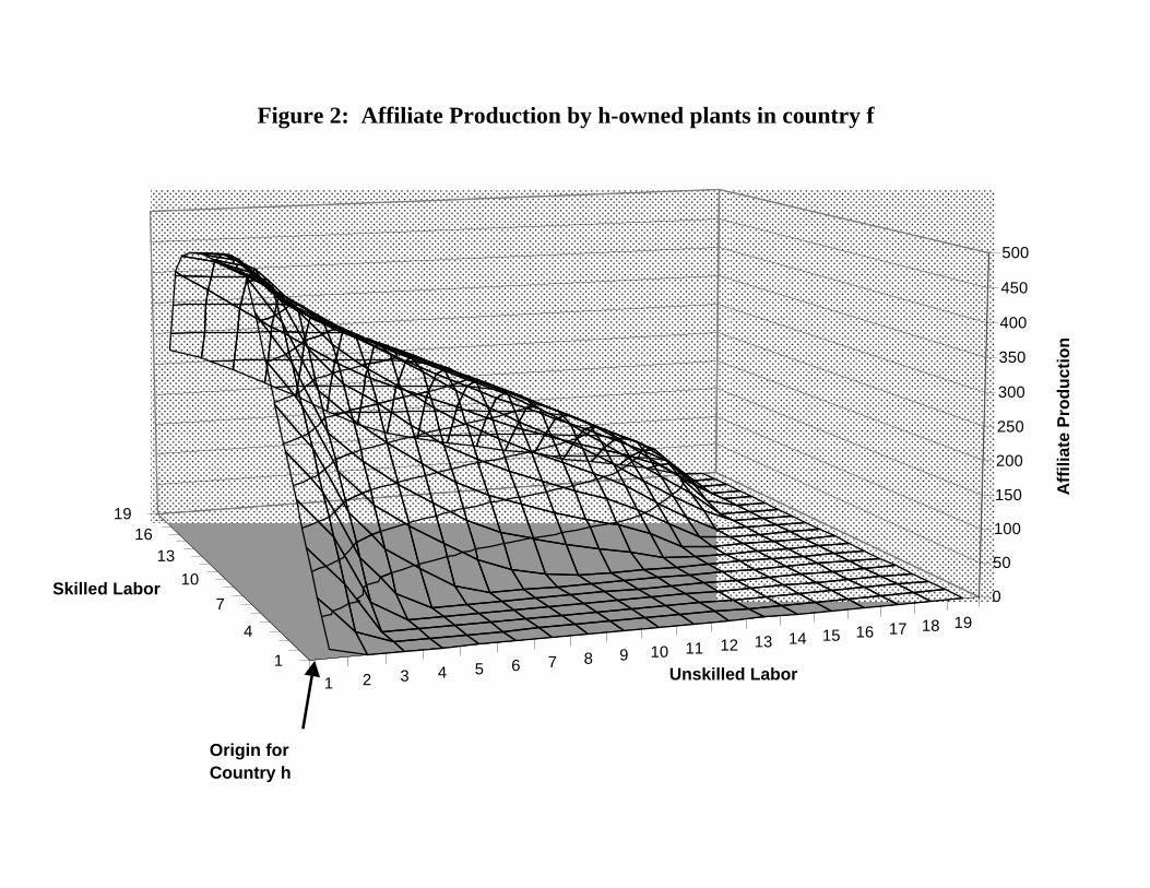
Figure 2 plots only the production by h-owned plants in country f. Here again, we see the

inverted u-shaped curve of production along the SW-NE diagonal, but affiliate production is

highest when country h is moderately small and highly skilled-labor abundant. The latter situation

is especially reminiscent of Sweden, Switzerland, and The Netherlands, which are small, skilled-

labor-abundant countries and important parent countries for multinationals.

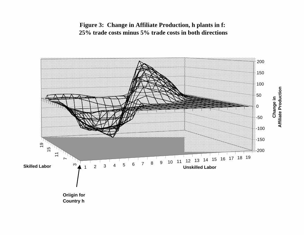
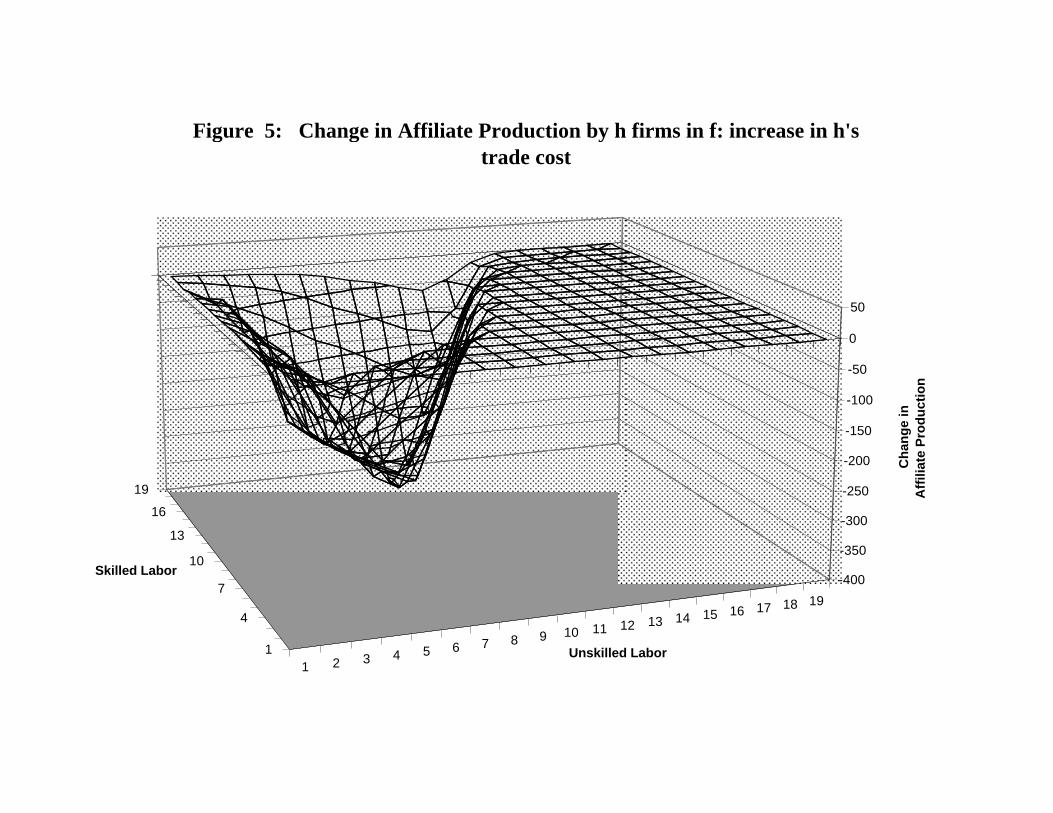
Figures 3 through 5 present results concerning the effects of trade costs, assumed here to

be symmetric in both directions, on production by h-owned plants in country f. On the vertical

axes of these diagrams is affiliate sales with 25% trade costs minus affiliate sales with 5% trade

costs. Again, we see that the results are highly non-linear. Figure 3 demonstrates that higher

trade costs increase total affiliate sales if the countries are relatively similar in size and in relative

12

endowments. Similarity favors horizontal multinationals and, as we noted earlier, horizontal

production is encouraged by higher trade costs. Higher trade costs, however, reduce total

affiliate sales when there is a moderate difference in relative endowments and the skilled-labor-

abundant country is somewhat smaller. These are regions with type-v firms headquartered in the

skilled-labor-abundant country and with a correspondingly large volume of X trade. Higher trade

costs "bring some plants back home" to the skilled-labor abundant country. In the NW region of

negative change in Figure 3, for example, higher trade costs lead to a substitution of some type-nh

firms for some type-vh firms, thereby reducing the volume of affiliate production. Parenthetically,

these are regions in which trade and affiliate sales are complements, in that higher trade costs

reduce both.

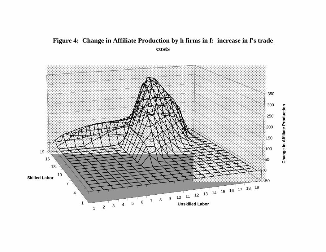
The results in Figure 3 are derived for an equal increase in trade costs in both directions.

This is not a very useful experiment to take to the data. Fortunately, the results break down

nicely into the effects of trade costs in the host country f and the trade costs to enter the parent

country h. These results are shown in Figures 4 and 5. Figure 4 shows that one effect of higher

trade costs in country f is to increase production of affiliates of country h firms in f if the countries

are relatively similar (horizontal investments). Figure 5 shows that the effect of increased trade

costs into the parent-country h is to discourage vertical investments in which the output of the

plant in country f is shipped back to country h. This impact occurs when h is relatively small and

skilled-labor abundant.

These various results lead us to specify the following central equation for estimation

purposes:

13

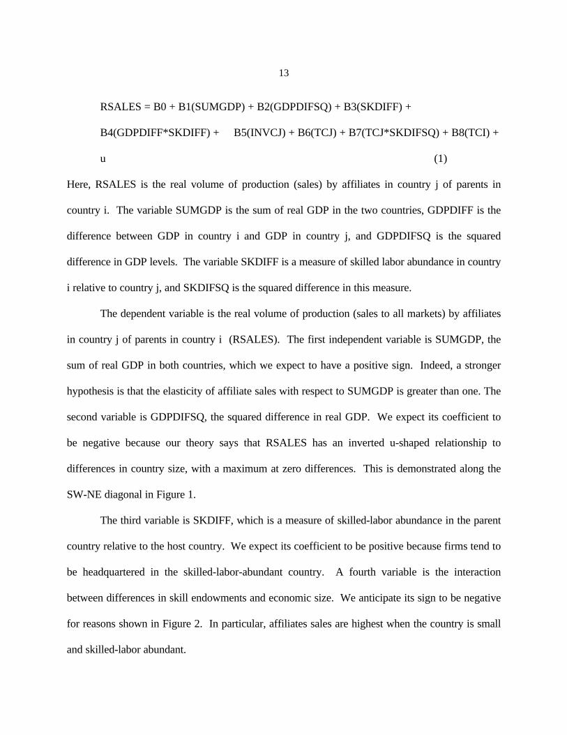
RSALES = B0 + B1(SUMGDP) + B2(GDPDIFSQ) + B3(SKDIFF) +

B4(GDPDIFF*SKDIFF) + B5(INVCJ) + B6(TCJ) + B7(TCJ*SKDIFSQ) + B8(TCI) +

u (1)

Here, RSALES is the real volume of production (sales) by affiliates in country j of parents in

country i. The variable SUMGDP is the sum of real GDP in the two countries, GDPDIFF is the

difference between GDP in country i and GDP in country j, and GDPDIFSQ is the squared

difference in GDP levels. The variable SKDIFF is a measure of skilled labor abundance in country

i relative to country j, and SKDIFSQ is the squared difference in this measure.

The dependent variable is the real volume of production (sales to all markets) by affiliates

in country j of parents in country i (RSALES). The first independent variable is SUMGDP, the

sum of real GDP in both countries, which we expect to have a positive sign. Indeed, a stronger

hypothesis is that the elasticity of affiliate sales with respect to SUMGDP is greater than one. The

second variable is GDPDIFSQ, the squared difference in real GDP. We expect its coefficient to

be negative because our theory says that RSALES has an inverted u-shaped relationship to

differences in country size, with a maximum at zero differences. This is demonstrated along the

SW-NE diagonal in Figure 1.

The third variable is SKDIFF, which is a measure of skilled-labor abundance in the parent

country relative to the host country. We expect its coefficient to be positive because firms tend to

be headquartered in the skilled-labor-abundant country. A fourth variable is the interaction

between differences in skill endowments and economic size. We anticipate its sign to be negative

for reasons shown in Figure 2. In particular, affiliates sales are highest when the country is small

and skilled-labor abundant.

14

The fifth and sixth variables, INVCJ and TCJ, respectively measure costs of investing in,

and exporting to, the host country. We expect the investment-cost coefficient to be negative and

the trade-cost coefficient to be positive. The interaction term between trade costs and squared

endowment differences is designed to capture the fact that trade costs may encourage horizontal

investment but not vertical investment and that horizontal investment is most important when

relative endowments are similar. The coefficient should therefore be negative, weakening the

direct effect of host-country trade costs. The results in Figure 4, however, show that the effect of

the host-country trade costs is not symmetric around the SW-NE diagonal and is actually highest

when the parent country is moderately skilled-labor abundant. Thus, this is not a theoretically

sharp hypothesis and, indeed, empirical support for this term is weak, as we shall see.

The final regressor is TCI, or trade costs in exporting to the parent country. The

coefficient should be negative because trade costs diminish the incentive to locate plants abroad

for shipment back to the home market, as shown in Figure 5. Figure 5 also indicates that TCI

should be interacted with SKDIFF, but the resulting variable is highly collinear with SKDIFF

because skilled-labor-scarce countries have high trade-cost indexes.5 Thus, we exclude this

interaction variable in the estimates provided here. Finally, in some versions of the econometric

model we add geographic distance, DIST, as an independent variable. The sign of this variable is

ambiguous in theory, because distance is an element in both export costs and investment and

monitoring costs. We specify the regression as linear in levels, with quadratic and interaction

terms included.

We may consider the sense of the interactive terms in more detail by writing the implied

5 The partial correlation coefficient between them is –0.96.

15

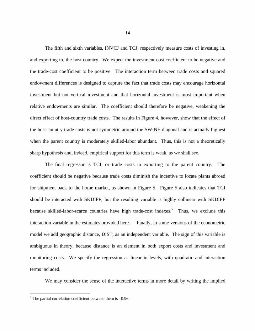
partial derivatives from equation (1). The derivative of RSALES with respect to TCJ has two

terms:

) SKDIFSQ( B + B = TCJ

RSALES 76

∂∂

Because B6 is greater than zero, this derivative is expected to be positive when relative endowments

are similar, reflecting the fact that host-country trade costs encourage horizontal direct investment. But

it should be smaller when relative endowments differ, in which case horizontal investment is less

important. This implies that the expected sign of B7 is negative.

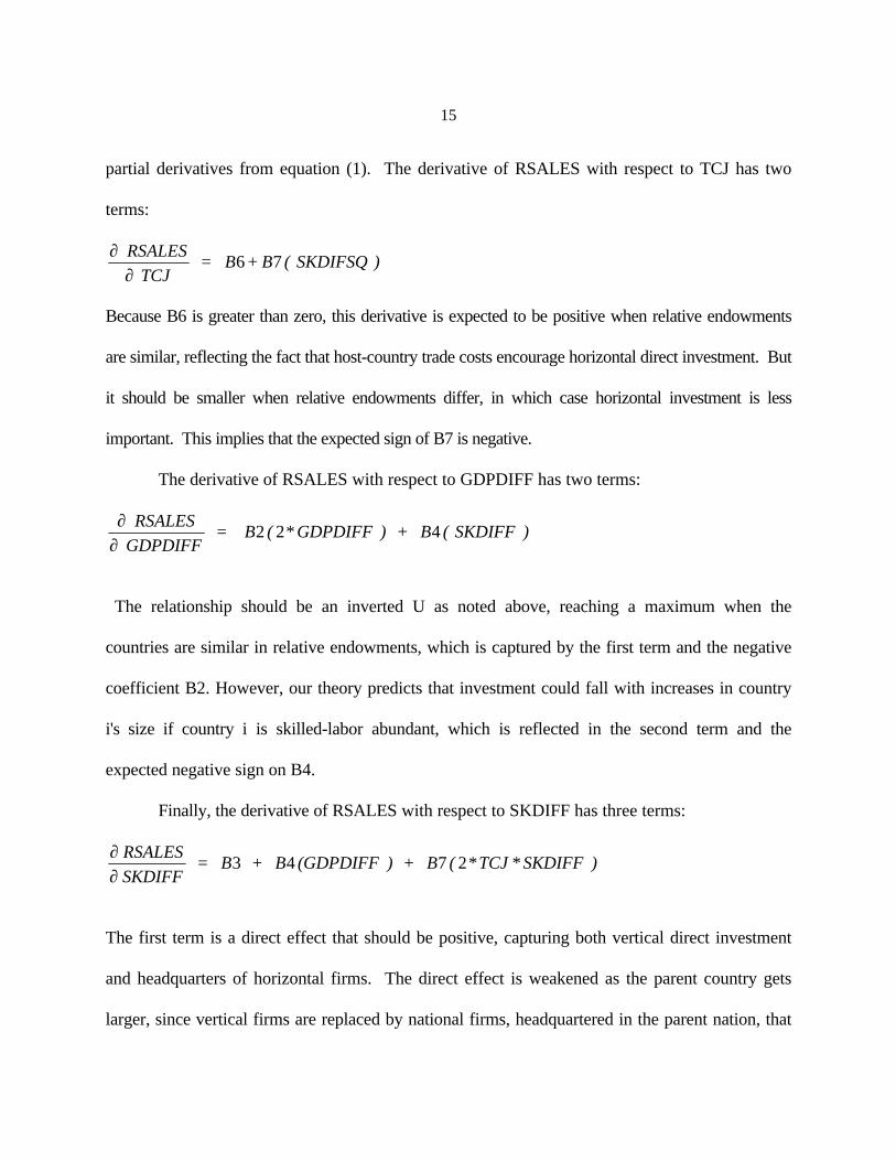
The derivative of RSALES with respect to GDPDIFF has two terms:

) SKDIFF( B + ) GDPDIFF ( B = GDPDIFF

RSALES 4*22

∂∂

The relationship should be an inverted U as noted above, reaching a maximum when the

countries are similar in relative endowments, which is captured by the first term and the negative

coefficient B2. However, our theory predicts that investment could fall with increases in country

i's size if country i is skilled-labor abundant, which is reflected in the second term and the

expected negative sign on B4.

Finally, the derivative of RSALES with respect to SKDIFF has three terms:

) SKDIFFTCJ ( B + ) (GDPDIFF B + B = SKDIFF

RSALES **2743

∂∂

The first term is a direct effect that should be positive, capturing both vertical direct investment

and headquarters of horizontal firms. The direct effect is weakened as the parent country gets

larger, since vertical firms are replaced by national firms, headquartered in the parent nation, that

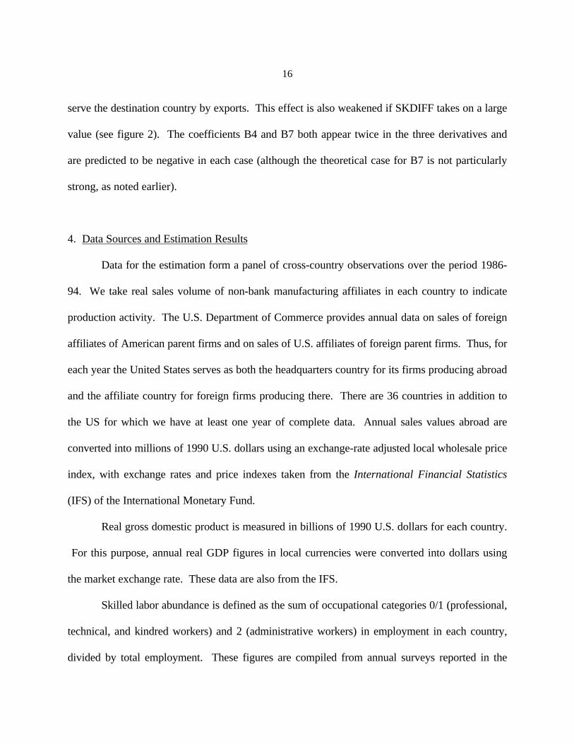
16

serve the destination country by exports. This effect is also weakened if SKDIFF takes on a large

value (see figure 2). The coefficients B4 and B7 both appear twice in the three derivatives and

are predicted to be negative in each case (although the theoretical case for B7 is not particularly

strong, as noted earlier).

4. Data Sources and Estimation Results

Data for the estimation form a panel of cross-country observations over the period 1986-

94. We take real sales volume of non-bank manufacturing affiliates in each country to indicate

production activity. The U.S. Department of Commerce provides annual data on sales of foreign

affiliates of American parent firms and on sales of U.S. affiliates of foreign parent firms. Thus, for

each year the United States serves as both the headquarters country for its firms producing abroad

and the affiliate country for foreign firms producing there. There are 36 countries in addition to

the US for which we have at least one year of complete data. Annual sales values abroad are

converted into millions of 1990 U.S. dollars using an exchange-rate adjusted local wholesale price

index, with exchange rates and price indexes taken from the International Financial Statistics

(IFS) of the International Monetary Fund.

Real gross domestic product is measured in billions of 1990 U.S. dollars for each country.

For this purpose, annual real GDP figures in local currencies were converted into dollars using

the market exchange rate. These data are also from the IFS.

Skilled labor abundance is defined as the sum of occupational categories 0/1 (professional,

technical, and kindred workers) and 2 (administrative workers) in employment in each country,

divided by total employment. These figures are compiled from annual surveys reported in the

17

Yearbook of Labor Statistics published by the International Labor Organization. In cases where

some annual figures were missing, the skilled-labor ratios were taken to equal the period averages

for each country. The variable SKDIFF is then simply the difference between the relative skill

endowment of the parent country and that of the affiliate country.

The cost of investing in the affiliate country is a simple average of several indexes of

impediments to investment, reported in the World Competitiveness Report of the World

Economic Forum.6 The indexes include restrictions on ability to acquire control in a domestic

company, limitations on the ability to employ foreign skilled labor, restraints on negotiating joint

ventures, strict controls on hiring and firing practices, market dominance by a small number of

enterprises, an absence of fair administration of justice, difficulties in acquiring local bank credit,

restrictions on access to local and foreign capital markets, and inadequate protection of

intellectual property. These indexes are computed on a scale from 0 to 100, with a higher number

indicating higher investment costs.

A trade cost index is taken from the same source and is defined as a measure of national

protectionism, or efforts to prevent importation of competitive products. It also runs from 0 to

100, with 100 being the highest trade costs. All of these indexes are based on extensive surveys

of multinational enterprises. We also incorporate a measure of distance, which is simply the

number of kilometers of each country's capital city from Washington, DC. It is unclear whether

this variable captures trade costs or investment costs, since both should rise with distance.

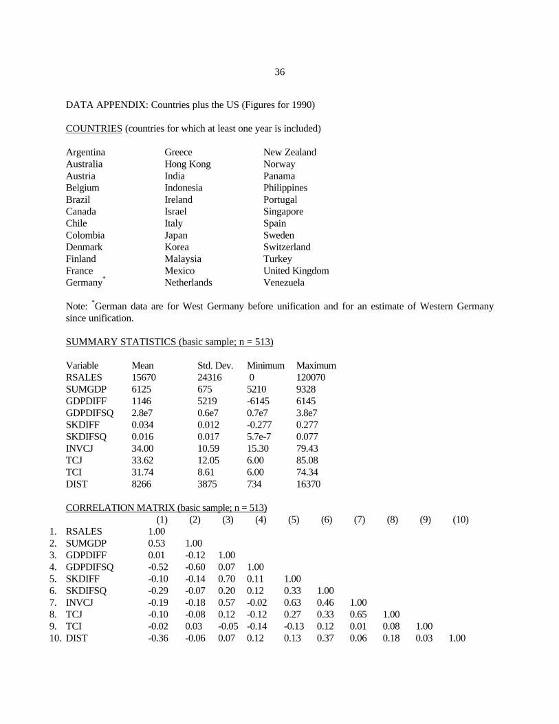
The Appendix lists the countries for which we have at least one complete yearly set of

6 Some of these data were kindly provided by staff of the United States International Trade Commission, whoused them in their report on trade liberalization (USITC, 1997).

18

observations, along with summary statistics. The final data set, after eliminating any row with

missing variables, contains 509 observations. An additional 119 observations are complete except

that no foreign affiliate sales are listed in the Commerce Department data. On examination, these

countries in all cases are relatively poor and generally small. Thus, we conjecture that the missing

observations are in fact zeros. We then perform alternative estimations using a Tobit procedure,

adding these cases to the data set for a total of 628 observations.

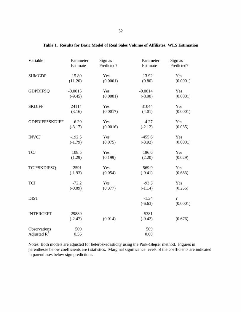
Results for the central-case regressions, excluding and including distance, are shown in

Tables 1 and 2. The regressions in Table 1 are estimated with a weighted least-squares

procedure, employing a Park-Glejser correction for heteroskedasticity. The first four variables

capture the relationships shown in Figures 1-3. All of the coefficients on these variables have the

hypothesized signs and are highly significant. Moreover, their magnitudes are relatively

insensitive to the inclusion of the distance variable in the second regression.

The next four variables involve the trade and investment cost measures. All signs are

consistent with the theory, although TCJ and TCI are insignificant in the first regression. Note

that adding distance, which in itself has a highly significant and negative impact on affiliate sales,

markedly raises the magnitude and significance of the investment-cost variable in the host country,

with a similar but smaller impact on the trade-cost variable.7 Thus, controlling for distance, the

decisions of multinational enterprises in setting output levels of affiliates are responsive to

perceived costs of investing in the country and the strength of import protection. This outcome is

sensible given our measures of investment costs and trade costs, which are indexes of perceived

7 It is not clear theoretically what the sign of the distance effect should be because distance may lead to a“substitution” effect toward investment and away from exports, but also generate a “scale” effect that decreasesboth trade and investment. The negative impact here is consistent with the finding of Brainard (1997).

19

costs and protectionism developed from surveys of multinational managers. The survey questions

do not ask about geographical distance, implying that the respondents do not factor it into their

answers. Thus, we have conceptually distinctive measures of distance and costs, although the

measures are correlated, as noted in the Appendix.

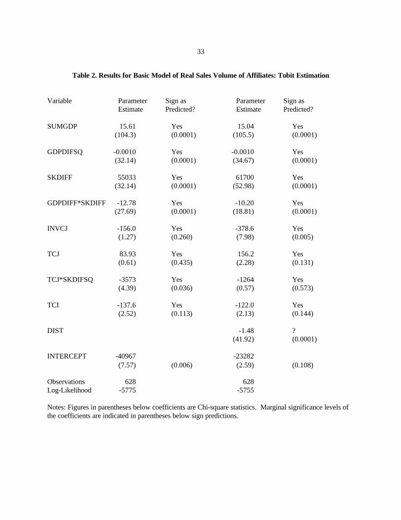
Results of the Tobit estimation are given in Table 2. Adding the cases with real sales

values of zero (ie, no affiliate activity) has virtually no impact on the SUMGDP and GDPDIFSQ

coefficients, but markedly increases the magnitudes of those on SKDIFF and GDPDIFF*SKDIFF,

while all four variables remain highly significant. The impact on the variables incorporating

differences in skilled-labor endowments is sensible because the zero-RSALES observations are

overwhelmingly cases where the potential parent nation is skilled-labor-scarce and smaller than

the potential affiliate nation (the United States). Excluding them from the WLS estimation in

Table 1 likely biases downward the role of skilled labor. This impact is seen also in the interaction

term between trade costs and squared skill differences, comparing the first columns of Tables 1

and 2. Finally, including distance in the Tobit regression has similar effects on the variables

incorporating trade costs and investment costs as it did in the WLS regression.

Overall, we believe the results in Tables 1 and 2 provide strong support to the knowledge-

capital model of foreign direct investment. Affiliate sales are strongly sensitive to bilateral

aggregate economic activity, squared differences in GDP, differences in skilled labor endowments,

and the interaction between size and endowment differences. The evidence suggests more weakly

that affiliate activity depends on investment costs and trade costs in the hypothesized directions.

We wish to use these results to characterize the various direct and indirect impacts more fully,

which is the next task.

20

5. Interpreting the coefficients

In this section, we interpret the magnitude of the coefficients and interpret the partial

derivatives discussed above. For this purpose, we employ the coefficients from the distance-

inclusive model in Table 1 and apply them to average data values from the year 1991.

First, consider increases in trade costs as measured by the index TCJ. It is clear from the

estimation that trade costs increase affiliate production when countries have identical relative

endowments of skilled labor (SKDIFF = 0). This is consistent with horizontal investment. How

large does the difference in relative endowments of skilled labor have to be in order to reverse the

sign of the derivative, so that an increase in TCJ leads to a fall in affiliate production (vertical

investment)? Recall that the variable SKDIFF is the difference between the proportion of the

labor force that is skilled in the parent country minus the proportion that is skilled in the affiliate

country. So a value of SKDIFF = 0.20, for example, could occur if country i has a skill ratio of

0.30 and country j has a skill ratio of 0.10. Results from Table 1 support the following

computation.

) SKDIFSQ( B + B = TCJ

RSALES 76

∂∂

(2)

= 196.6 – 569.9*SKDIFSQ > 0 iff SKDIFF < 0.587

In the data, no recorded difference in skill ratios exceeded this critical value. We can therefore state the

following empirical conclusion.

Result 1: An increase in the host-country's trade costs will raise production by affiliates of parent

country firms in all cases.

21

This result states that higher host-country trade costs always lead to more affiliate production

in that country, although large differences in relative endowments weaken the result. This finding is

thus roughly consistent with Figure 4, although in that diagram there are large areas in which the host-

country trade cost has no effect.

Second, consider an increase in country i's GDP, holding total world GPD constant (i.e,

country j's GPD change is the negative of country i's change). When countries have identical

relative endowments, this derivative is positive with GDPDIFF < 0, zero at GDPDIFF = 0, and

negative with GDPDIFF > 0. With country i more skilled-labor abundant than country j, the

theory and simulations predicted that this derivative switches sign, from positive to negative, at a

lower value of GDPDIFF (see Figure 2). Results from Table 1 (distance included) give us the

following results.

) SKDIFF( B + ) GDPDIFF (B = GDPDIFF

RSALES 4*22

∂∂

(3)

= - 0.0014*2*(GDPDIFF) - 4.3*(SKDIFF)

An increase in a country's GDP will increase its affiliate sales abroad only if it is small and/or

skilled-labor scarce.8

One interesting interpretation of these results involves the convergence in income between

the United States and its trading partners, holding total "world" income constant (SUMGDP is

constant). Using values of SKDIFF from the data, it turns out that the contribution of the last

term in Equation (3) is small and is always dominated by the first term. Note that GDPDIFF is

8 There are 66 country pairs (i,j observations) with positive affiliate sales from i to j in 1991. Fifty-nine of thesehave complete data for this exercise. Thirty-six of the 59 are affiliate sales of US firms in some country j and 23are country i affiliate sales in the US.

22

always positive if the US is country i and negative if the US is country j.

Result 2: A convergence in income (GDP) between the United States and country j (holding the

sum of their incomes constant) increases affiliate sales in both directions.

This result is connected to the theory in Figure 6, which plots affiliate production along the

SW-NE diagonal of the factor box (countries differ in size but have identical relative endowments)

from Figure 1. Affiliate production by h-owned firms in f (see Figure 2) and f-owned firms in h are

plotted separately in Figure 6. The larger country always has a larger share of total affiliate sales

except when the countries are extremely different in size.9 Note that there are regions of relative size,

ranging from 0.25 to 0.40 and from 0.60 to 0.75, where a convergence in country size toward the

center of the box increases affiliate sales in both directions. This occurs when the difference in country

size is "moderately large but not too large". Our empirical results emphasize the relevance of this

result.

Third, consider an increase in the skilled-labor abundance of country i relative to country j.

Our results in Table 1 indicate that this derivative is generally positive for similar countries, but

its (absolute) value is reduced by a higher relative endowment difference or a larger GPD

difference.

) SKDIFFTCJ( B7 + ) (GDPDIFF B + B = SKDIFF

RSALES **243

∂∂

(4)

= 31044 – 4.3*(GDPDIFF) – 569.9*2*(TCJ*SKDIFF)

9 When the countries are extremely different in size, all production is in the large country, most of which is bysingle-plant national firms headquartered in the large country. But this situation leaves the price of skilled laborlow in the small country, inducing a few firms to place headquarters there. Thus, production abroad is affiliatesales of small-country firms in the large country.

23

Large values of SKDIFF and GDPDIFF weaken the effects of an increase in skilled-labor

abundance on outward affiliate sales.

Inserting values for SKDIFF, TCJ and GDPDIFF for the 1991 data, these results imply the

following.

Result 3: An increase in the parent country's skilled labor abundance relative to the host country

increases affiliate sales from the parent to the host except when the US is parent and the host is India,

Indonesia, Republic of Korea, Malaysia, or Philippines.

These exceptions are cases where the US (the parent) is highly skilled-labor abundant relative

to the host. This result connects to the theory as shown in Figure 7, which graphs affiliate sales by h-

owned firms in country f, as country h's share of world skilled labor varies, holding each country's share

of unskilled labor at one-half (i.e., this represents the cells above column “10” of Figure 2). At low

levels of skilled labor, country h has no affiliate sales. These eventually become positive, but then

finally fall as country f becomes very skilled-labor scarce. Even the modest skilled-labor requirements

in plant fixed costs become too expensive in country f and both production and headquarters are

concentrated in country h. The developing- country exceptions to the outcome in Result 3 are

consistent with the right-hand end of Figure 7, where further increases in country h's skilled-labor

abundance lead to a fall in affiliate sales.

As a final point, we note that the theory suggests a sharper hypothesis on the coefficient of

SUMGDP than that it is simply positive. Higher total income should lead to some shifting from

national firms, which are high marginal-cost suppliers to foreign markets, to horizontal

multinationals, which are high fixed-cost suppliers (Markusen and Venables, 1998). In regions of

parameter space in which regime shifting does not occur, affiliate production should rise in

24

proportion to total world income. Overall, this suggests that affiliate sales should be elastic with

respect to world income. We therefore used the results to calculate the implied elasticity of total

affiliate sales (RSALES) with respect to total income (SUMGDP) for 1991 in the data. The

result is an elasticity of 5.35: an increase of world real income of 1% results in an estimated

5.35% increase in affiliate sales, other things equal. This finding further supports the underlying

theory.

6. Further Econometrics

The results presented above are from a panel data set and it is of interest to decompose

them into cross-section and time-series effects. Before discussing this, we emphasize that the

theoretical results apply equally well to time-series and cross-section processes. That is, the

theory should correctly characterize both the time-path of the interactions between two countries

and the interactions among countries in a single year. For example, as two countries grow in total

GDP and become more similar in size over time, direct investment between them should grow in

the manner suggested by the theory. Among a set of countries in a given year, the same bilateral

relationships should apply.

One way to isolate the cross-section contribution to the results is to use single-year

regressions or to average the years for each variable. We have done the latter, but the procedure

generates a severe multicollinearity problem due to the bilateral nature of the data, with the

United States always being one of the two countries in each data point (the same problem would

occur for individual years). The resulting data set has only 63 observations.

The principal difficulty is that SUMGDP and GDPDIFSQ are highly collinear: they have a

25

correlation coefficient of 0.995 in our cross section. The time-series variation in U.S. GDP is

vital to identifying the separate contributions of these two variables and this information is

discarded in the averaging procedure (or in the use of a single year). We can partially reduce this

problem by using the non-U.S. country’s GDP (NGDP) in place of SUMGDP and that country’s

squared GDP (GDPNSQ) in place of GDPDIFSQ (regardless of whether the United States is the

source or host country). Then the U.S. GDP in each observation is blended into the constant

term. Since the United States is always the larger country, the theory tells us that the coefficient

on GDPN should be positive, regardless of whether country N is the source or host nation

(catching up to the United States increases investment in both directions). The hypothesized

negative coefficient on GDPNSQ is the diminishing effect of increasing country N’s GDP (the

theory says that eventually further increases in GDPN will reduce investment in both directions).

A second problem is that there is far less independent information than would appear with

63 observations. The variable TCI has the same value for all U.S. outward investments and TCJ

and INVCJ have the same values for all investments in the United States. The three variables

GDPN, GDPNSQ, and GDPDIFF*SKDIFF have the same values for U.S. investments in country

N and country N investments in the United States. The variables GDPN and GDPNSQ still have

a correlation of 0.93. Despite these difficulties, we report results for the averaged cross-section in

Table 3, with the distance variable included. This regression corresponds to the second one in

Table 1, except that the coefficients on GDPN, GDPNSQ, and the intercept in Table 3 cannot be

compared to those on SUMGDP, GDPDIFSQ, and the intercept in the former table.

Not surprisingly, the standard errors are large, given the problems just mentioned. The

coefficients on TCJ, TCI, and GDPDIFF*SKDIFF are insignificant, as is the coefficient on

26

TCJ*SKDIFSQ. However, only the coefficient on TCJ*SKDIFSQ has the wrong sign.

Statistical significance aside, the magnitude of the coefficients for SKDIFF, and INVCJ are not

much different in the two tables.

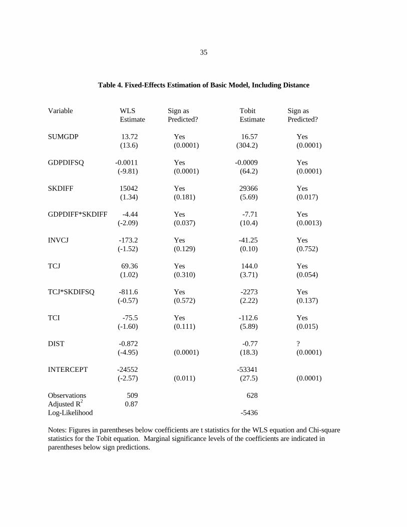
To distinguish the time-series contributions to the results we employ country fixed effects.

Table 4 lists results where the equation contains a dummy variable for each country (regardless if

it is the source or recipient country in a given observation) except the United States. The first

regression employs WLS and the second is the related Tobit estimation. We do not report the

coefficients of the country dummies, but most are significant.10

The results are qualitatively similar to those in Table 1 for the first group of four variables,

except that the coefficient on SKDIFF is reduced by half. The magnitudes of the coefficients on

INVCJ and TCJ are considerably smaller in Table 4 as well and both have lower significance

levels. Thus, although the sign pattern is robust to the inclusion of country fixed effects, it is

difficult to identify confidently the contribution of trade costs and investment costs to

multinational production.

The Tobit results also show a smaller coefficient for SKDIFF with the country dummies

added. The variables measuring perceived trade costs are significant in this specification in the

hypothesized directions, but the investment-cost variable is not. Overall, it appears that the

addition of country fixed effects does not change the results qualitatively, but a smaller role for

endowment differences is predicted.11 It is noteworthy that in the Tobit specification, which

10 Results are available on request. We also tried country-pair dummies but with the United States as a partner ineach case this procedure could not well distinguish individual country effects.11 Most of the countries in the sample are less skilled-labor-abundant than the United States. It may be that thecountry dummies are capturing some of this effect that should be correctly attributed to endowment differences, asit is in the panel and in the cross-section.

27

incorporates many more developing countries with zero reported affiliate sales, the magnitudes

and significance levels of trade costs in both host and parent countries are expanded, as are those

of relative endowment differences. This result provides some support for the notion that

horizontal and vertical FDI respond differently to host-country and parent-country trade

protection.

7. Summary

The knowledge-capital approach to the multinational enterprise as outlined in this paper is

operational and yields clear, testable hypotheses. It this sense, it is more useful that some other

theories of FDI, such as the "transactions cost" approach to multinational enterprises.

In this paper, we test hypotheses regarding the importance of multinational activity

between countries as a function of certain characteristics of those countries, particularly size, size

differences, relative endowment differences, trade and investment costs, and certain interactions

among these variables as predicted by the theory. In our view, the model fits well and gives

considerable support to the theory. The panel estimates in Tables 1 and 2 yield correct signs and

strong statistical significance (when distance is included) for the central variables SUMGPD,

GDPDIFSQ, SKDIFF, GDPDIFF*SKDIFF, INVCJ, and TCJ. Other variables (TCI and

TCJ*SKDIFSQ) have correct signs but display weak statistical significance. Our efforts to separate

the panel results into cross-section and time-series impacts are made problematic by multicollinearity in

the cross-section data. Because of the bilateral nature of these data, the time-series variation in the

U.S. observations is critical to identification of the contributions of several variables. Estimation with

28

country fixed effects produced results consistent with the panel approach.12

According to our findings, outward investment from a source country to affiliates in a host

country is increasing in the sum of their economic sizes, their similarity in size, the relative skilled-labor

abundance of the parent nation, and the interaction between size and relative endowment differences.

Some of these findings are consistent with earlier results, particularly those of Brainard (1993) and

Ekholm (1997b). But the precise formulations here are different and closely tied to one particular

model. This model allows for simultaneous horizontal and vertical motives for direct investment and

emphasizes certain interactions, such as that between size and endowment differences. We should also

note that the theoretical model fully endogenizes trade flows in its calculations, allowing direct

predictions on affiliate sales without requiring us to worry about questions of trade versus investment.

Trade, like factor and commodity prices, is endogenous in generating the predictions of the model.

Subsequent to the estimation, we interpreted the estimates in the language of comparative-

statics questions about the world economy. Results indicate first that increases in host-country trade

costs will increase inward affiliate production, second that a convergence in country size between the

US and country i will increase affiliate sales in both directions, and third that an increase in a country's

skilled-labor abundance will increase outward affiliate sales for almost all country pairs.

In summary, we are enthusiastic about the results, and hope that the model will therefore prove

useful in future policy analysis.

12 For comparison purposes, we ran a simple gravity equation on the panel data set, with log real affiliate salesregressed on log real GDP in host and parent countries and log distance. The gravity equation displayed aconsiderably lower adjusted R2 (0.46) than the panel equation based on the theoretical model (0.60).

29

REFERENCES

Aitken, Brian, Ann Harrison, and Robert E. Lipsey (1995), "Wages and Foreign Ownership: AComparative Study of Mexico, Venezuela, and the United States", NBER working paper5102.

Blomstrom, Magnus, Gunnar Fors, and Robert E. Lipsey, "Foreign Direct Investment andEmployment: Home Country Experience in the United States and Sweden", NBERworking paper 6205, 1997.

Brainard, S. Lael, "A Simple Theory of Multinational Corporations and Trade with a Trade-offbetween Proximity and Concentration", NBER Working Paper No. 4269, February 1993a.

Brainard, S. Lael, "An Empirical Assessment of the Factor Proportions Explanation ofMultinationals Sales", NBER Working Paper No. 4580, December 1993b.

Brainard, S. Lael, "An Empirical Assessment of the Proximity-Concentration Tradeoff betweenMultinational Sales and Trade", American Economic Review,1997, 87, 520-544.

Braunerhjelm, Pontus and Karolina Ekholm (editors), The Geography of Multinational Firms.Boston: Kluwer Academic Publishers. 1998.

Caves, Richard E., Multinational Enterprise and Economic Analysis. London: CambridgeUniversity Press. 1996, second edition.

Ekhlom, Karolina, Multinational Production and Trade in Technological Knowledge, LundEconomic Studies, number 58, 1995.

Ekholm, Karolina, "Headquarter Services and Revealed Factor Abundance", Review ofInternational Economics, 1997a.

Ekholm, Karolina, "Factor Endowments and the Pattern of Affiliate Production by MultinationalEnterprises", CREDIT working paper no. 97/19, University of Nottingham, 1997b.

Ekholm, Karolina, "Proximity Advantages, Scale Economies, and the Location of Production", inBraunerhjelm and Ekholm (editors), The Geography of Multinational Firms. Boston:Kluwer Academic Publishers. 1998.

Feenstra, Robert C. and Gordon H. Hanson, "Foreign Direct Investment and Relative Wages:Evidence from Mexico's Maquiladoras", Journal of International Economics 1997, 42,371-393.

Helpman, Elhanan, "A Simple Theory of Trade with Multinational Corporations", Journal of

30

Political Economy, 1984, 92, 451-471.

Helpman, Elhanan, "Multinational Corporations and Trade Structure", Review of EconomicStudies, 1985, 52, 443-458.

Horstmann, Ignatius J. and James R. Markusen, "Strategic Investments and the Development ofMultinationals," International Economic Review, 1987, 28, 109-121.

Horstmann, Ignatius J. and James R. Markusen, "Endogenous Market Structures in InternationalTrade," Journal of International Economics, 1992, 32, 109-129.

Lipsey, Robert E., Magnus Blomstrom and Eric Ramstetter, "Internationalized Production inWorld Output", NBER working paper 5385, 1995.

Markusen, James R., "Multinationals, Multi-Plant Economies, and the Gains from Trade", Journalof International Economics 1984, 16, 205-226.

Markusen, James R., "The Boundaries of Multinational Firms and the Theory of InternationalTrade", Journal of Economic Perspectives 1995, 9, 169-189.

Markusen, James R., "Trade versus Investment Liberalization", NBER working paper 6231,1997.

Markusen, James R. and Anthony J. Venables, "The Increased Importance of Multinationals inNorth American Economic Relationships: A Convergence Hypothesis", in Canzoneri,Matthew W.,Wilfred J. Ethier, and Vitoria Grilli (editors), The New TransatlanticEconomy, London: Cambridge University Press, 1996.

Markusen, James R. and Anthony J. Venables, "The Role of Multinational Firms in the Wage-GapDebate", Review of International Economics 1997, 5, 435-451.

Markusen, James R. and Anthony J. Venables, "Multinational Firms and the New Trade Theory",Journal of International Economics 1998 forthcoming.

Markusen, James R., Anthony J. Venables, Denise Eby Konan, and Kevin Zhang, "A UnifiedTreatment of Horizontal Direct Investment, Vertical Direct Investment, and the Pattern ofTrade in Goods and Services", NBER working paper 5696, 1996.

Rutherford, Thomas F., "Applied General-Equilibrium Modelling with MPS/GE as a GAMSSubsystem" 1995a.

Rutherford, Thomas F., "Extensions of GAMS for Complementarity Problems Arising in AppliedEconomics", Journal of Economic Dynamics and Control 1995b.

31

Slaughter, Matthew J., "Multinational Corporations, Outsourcing, and American Relative WageDivergence", Journal of International Economics 1999 forthcoming.

UNCTAD, World Investment Report, 1993.

32

Table 1. Results for Basic Model of Real Sales Volume of Affiliates: WLS Estimation

Variable Parameter Sign as Parameter Sign asEstimate Predicted? Estimate Predicted?

SUMGDP 15.80 Yes 13.92 Yes(11.20) (0.0001) (9.80) (0.0001)

GDPDIFSQ -0.0015 Yes -0.0014 Yes(-9.45) (0.0001) (-8.90) (0.0001)

SKDIFF 24114 Yes 31044 Yes(3.16) (0.0017) (4.01) (0.0001)

GDPDIFF*SKDIFF -6.20 Yes -4.27 Yes(-3.17) (0.0016) (-2.12) (0.035)

INVCJ -192.5 Yes -455.6 Yes(-1.79) (0.075) (-3.92) (0.0001)

TCJ 108.5 Yes 196.6 Yes(1.29) (0.199) (2.20) (0.029)

TCJ*SKDIFSQ -2591 Yes -569.9 Yes(-1.93) (0.054) (-0.41) (0.683)

TCI -72.2 Yes -93.3 Yes(-0.89) (0.377) (-1.14) (0.256)

DIST -1.34 ?(-6.63) (0.0001)

INTERCEPT -29889 -5381(-2.47) (0.014) (-0.42) (0.676)

Observations 509 509Adjusted R2 0.56 0.60

Notes: Both models are adjusted for heteroskedasticity using the Park-Glejser method. Figures inparentheses below coefficients are t statistics. Marginal significance levels of the coefficients are indicatedin parentheses below sign predictions.

33

Table 2. Results for Basic Model of Real Sales Volume of Affiliates: Tobit Estimation

Variable Parameter Sign as Parameter Sign asEstimate Predicted? Estimate Predicted?

SUMGDP 15.61 Yes 15.04 Yes(104.3) (0.0001) (105.5) (0.0001)

GDPDIFSQ -0.0010 Yes -0.0010 Yes(32.14) (0.0001) (34.67) (0.0001)

SKDIFF 55033 Yes 61700 Yes(32.14) (0.0001) (52.98) (0.0001)

GDPDIFF*SKDIFF -12.78 Yes -10.20 Yes(27.69) (0.0001) (18.81) (0.0001)

INVCJ -156.0 Yes -378.6 Yes(1.27) (0.260) (7.98) (0.005)

TCJ 83.93 Yes 156.2 Yes(0.61) (0.435) (2.28) (0.131)

TCJ*SKDIFSQ -3573 Yes -1264 Yes(4.39) (0.036) (0.57) (0.573)

TCI -137.6 Yes -122.0 Yes(2.52) (0.113) (2.13) (0.144)

DIST -1.48 ?(41.92) (0.0001)

INTERCEPT -40967 -23282(7.57) (0.006) (2.59) (0.108)

Observations 628 628Log-Likelihood -5775 -5755

Notes: Figures in parentheses below coefficients are Chi-square statistics. Marginal significance levels ofthe coefficients are indicated in parentheses below sign predictions.

34

Table 3. Cross-Section Estimation of Basic Model, Including Distance

Variable WLS Sign as Tobit Sign as Estimate Predicted? Estimate Predicted?

GDPN 65.51 Yes 66.38 Yes(5.74) (0.0001) (46.7) (0.0001)

GDPNSQ -0.018 Yes -0.018 Yes(-3.72) (0.0001) (24.1) (0.0001)

SKDIFF 27176 Yes 49834 Yes(1.29) (0.204) (5.17) (0.023)

GDPDIFF*SKDIFF -2.41 Yes -8.42 Yes (-0.39) (0.702) (1.65) (0.199)

INVCJ -462.3 Yes -526.5 Yes(-1.23) (0.223) (1.83) (0.176)

TCJ 4.11 Yes -48.5 No(0.01) (0.990) (0.02) (0.891)

TCJ*SKDIFSQ 1085 No 2375 No(0.24) (0.812) (0.26) (0.616)

TCI -125.5 Yes -95.2 Yes(-0.54) (0.595) (0.16) (0.689)

DIST -0.55 ? -0.65 ?(-1.02) (0.314) (1.29) (0.256)

INTERCEPT 21861 25862(1.54) (0.130) (3.29) (0.070)

Observations 63 70Adjusted R2 0.60Log-Likelihood -687.0

Notes: Model uses average observations for each country pair. WLS equation is adjusted forheteroskedasticity using the Park-Glejser method. Figures in parentheses below coefficients are t- statisticsfor the WLS equation and Chi-square statistics for the Tobit equation. Marginal significance levels of thecoefficients are indicated in parentheses below sign predictions.

35

Table 4. Fixed-Effects Estimation of Basic Model, Including Distance

Variable WLS Sign as Tobit Sign asEstimate Predicted? Estimate Predicted?

SUMGDP 13.72 Yes 16.57 Yes(13.6) (0.0001) (304.2) (0.0001)

GDPDIFSQ -0.0011 Yes -0.0009 Yes(-9.81) (0.0001) (64.2) (0.0001)

SKDIFF 15042 Yes 29366 Yes(1.34) (0.181) (5.69) (0.017)

GDPDIFF*SKDIFF -4.44 Yes -7.71 Yes(-2.09) (0.037) (10.4) (0.0013)

INVCJ -173.2 Yes -41.25 Yes(-1.52) (0.129) (0.10) (0.752)

TCJ 69.36 Yes 144.0 Yes(1.02) (0.310) (3.71) (0.054)

TCJ*SKDIFSQ -811.6 Yes -2273 Yes(-0.57) (0.572) (2.22) (0.137)

TCI -75.5 Yes -112.6 Yes(-1.60) (0.111) (5.89) (0.015)

DIST -0.872 -0.77 ?(-4.95) (0.0001) (18.3) (0.0001)

INTERCEPT -24552 -53341(-2.57) (0.011) (27.5) (0.0001)

Observations 509 628Adjusted R2 0.87Log-Likelihood -5436

Notes: Figures in parentheses below coefficients are t statistics for the WLS equation and Chi-squarestatistics for the Tobit equation. Marginal significance levels of the coefficients are indicated inparentheses below sign predictions.

36

DATA APPENDIX: Countries plus the US (Figures for 1990)

COUNTRIES (countries for which at least one year is included)

Argentina Greece New ZealandAustralia Hong Kong NorwayAustria India PanamaBelgium Indonesia PhilippinesBrazil Ireland PortugalCanada Israel SingaporeChile Italy SpainColombia Japan SwedenDenmark Korea SwitzerlandFinland Malaysia TurkeyFrance Mexico United KingdomGermany* Netherlands Venezuela

Note: *German data are for West Germany before unification and for an estimate of Western Germanysince unification.

SUMMARY STATISTICS (basic sample; n = 513)

Variable Mean Std. Dev. Minimum MaximumRSALES 15670 24316 0 120070SUMGDP 6125 675 5210 9328GDPDIFF 1146 5219 -6145 6145GDPDIFSQ 2.8e7 0.6e7 0.7e7 3.8e7SKDIFF 0.034 0.012 -0.277 0.277SKDIFSQ 0.016 0.017 5.7e-7 0.077INVCJ 34.00 10.59 15.30 79.43TCJ 33.62 12.05 6.00 85.08TCI 31.74 8.61 6.00 74.34DIST 8266 3875 734 16370

CORRELATION MATRIX (basic sample; n = 513)(1) (2) (3) (4) (5) (6) (7) (8) (9) (10)

1. RSALES 1.002. SUMGDP 0.53 1.003. GDPDIFF 0.01 -0.12 1.004. GDPDIFSQ -0.52 -0.60 0.07 1.005. SKDIFF -0.10 -0.14 0.70 0.11 1.006. SKDIFSQ -0.29 -0.07 0.20 0.12 0.33 1.007. INVCJ -0.19 -0.18 0.57 -0.02 0.63 0.46 1.008. TCJ -0.10 -0.08 0.12 -0.12 0.27 0.33 0.65 1.009. TCI -0.02 0.03 -0.05 -0.14 -0.13 0.12 0.01 0.08 1.0010. DIST -0.36 -0.06 0.07 0.12 0.13 0.37 0.06 0.18 0.03 1.00

1 2 3 4 5 6 7 8 9 10 11 12 13 14 15 16 17 18 19

19

15

11

7

3

0

50

100

150

200

250

300

350

400

450

500

Aff

iliat

e P

rod

uct

ion

Unskilled Labor

Skilled Labor

Figure 1: Volume of Affliate Production: 25% trade costs

Origin for Country h

Approximate locus of equal incomes for h and f

1 2 3 4 5 6 7 8 9 10 11 12 13 14 15 16 17 18 19

1916

13

10

7

4

1

0

50

100

150

200

250

300

350

400

450

500

Aff

iliat

e P

rod

uct

ion

Unskilled Labor

Skilled Labor

Figure 2: Affiliate Production by h-owned plants in country f

Origin for Country h

1 2 3 4 5 6 7 8 9 10 11 12 13 14 15 16 17 18 19

19

15

11

7

3

-200

-150

-100

-50

0

50

100

150

200

Ch

ang

e in

A

ffili

ate

Pro

du

ctio

n

Unskilled LaborSkilled Labor

Figure 3: Change in Affiliate Production, h plants in f: 25% trade costs minus 5% trade costs in both directions

Oriigin for Country h

1 2 3 4 5 6 7 8 9 10 11 12 13 14 15 16 17 18 19

19

16

13

10

7

4

1

-50

0

50

100

150

200

250

300

350

Ch

ang

e in

Aff

iliat

e P

rod

uct

ion

Unskilled Labor

Skilled Labor

Figure 4: Change in Affiliate Production by h firms in f: increase in f's trade costs

1 2 3 4 5 6 7 8 9 10 11 12 13 14 15 16 17 18 19

19

16

13

10

7

4

1

-400

-350

-300

-250

-200

-150

-100

-50

0

50

Ch

ang

e in

A

ffili

ate

Pro

du

ctio

n

Unskilled Labor

Skilled Labor

Figure 5: Change in Affiliate Production by h firms in f: increase in h's trade cost

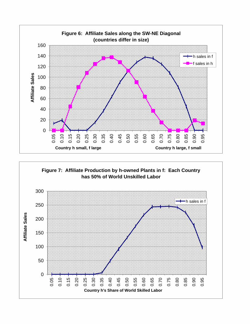
Figure 6: Affiliate Sales along the SW-NE Diagonal (countries differ in size)

0

20

40

60

80

100

120

140

160

0.05

0.10

0.15

0.20

0.25

0.30

0.35

0.40

0.45

0.50

0.55

0.60

0.65

0.70

0.75

0.80

0.85

0.90

0.95

Country h small, f large Country h large, f small

Aff

iliat

e S

ales

h sales in f

f sales in h

Figure 7: Affiliate Production by h-owned Plants in f: Each Country has 50% of World Unskilled Labor

0

50

100

150

200

250

300

0.05

0.10

0.15

0.20

0.25

0.30

0.35

0.40

0.45

0.50

0.55

0.60

0.65

0.70

0.75

0.80

0.85

0.90

0.95

Country h's Share of World Skilled Labor

Aff

iliat

e S

ales

h sales in f

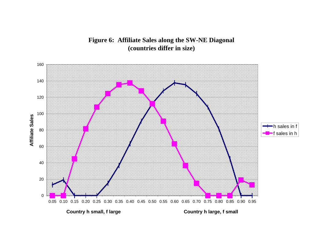
Figure 6: Affiliate Sales along the SW-NE Diagonal (countries differ in size)

0

20

40

60

80

100

120

140

160

0.05 0.10 0.15 0.20 0.25 0.30 0.35 0.40 0.45 0.50 0.55 0.60 0.65 0.70 0.75 0.80 0.85 0.90 0.95

Country h small, f large Country h large, f small

Aff

iliat

e S

ales

h sales in ff sales in h