The Incidence of Social SecurityContributions: Evidence from German

Administrative Data

Michael Neumann

German Institute for Economic Research (DIW Berlin)

mneumann@diw.de

February 15, 2013

Preliminary - comments welcome

Abstract

This paper applies a test for the incidence of social security contributions based on

the reaction of gross wages in response to a variation in social security contributions.

Exploiting an increase of the East German taxable maximum of health insurance, a

difference-in-differences approach is used to estimate its effects on yearly changes in

gross wages. It is shown that employees earning somewhat less than the taxable maxi-

mum represent a valid control goup. Based on the resulting confidence interval bounds

of burden shifting supported by the data are calculated. I find that considerable shifting

in any direction can be rejected.

1

1 Introduction

Especially in Germany social security contributions (SSC) represent a large share of to-

tal taxation, thus playing an important role in financing government spending. In 2010,

SSCs amounted to 15.8 percent of German GDP and 40 percent of total tax revenues 1.

A special feature of SSCs in Germany and many other countries is that the burden is

statutorily shared between employers and employees. Particularly the employer’s share

is often accused to be detrimental to employment by raising the cost of labour. This

was a major motivation of several reforms in Germany aiming to relieve employers in

order to boost employment. In 2005, the equal share between employers and employees

was abolished by introducing a contribution of 0.9 percentage points which has to be

exclusively paid by employees. Furthermore, childless employees had to pay additional

0.25 percentage points. These reforms implicitly assumed that it matters who formally

bears the burden of SSCs. However, economic theory often finds or assumes that the

formal organisiation of a tax does not play a role (invariance of incidence proposition).

This paper empirically analyses the question of who is economically made worse off by

an increase of SSCs.

To do that, a test for the incidence based on gross wages is applied. Assume SSCs

are equally increased for employees and employers. Ceteris paribus, labour costs (gross

wages + employers’ SSCs) increase, gross wages are not affected and net wages (gross

wages - employees’ SSCs) decrease. The economic burden of this increase in SSC can

then be shifted to the respective other party by adjusting the gross hourly wage. An

increase of gross hourly wages would attentuate the depressing effect on net wages at

the cost of even higher labour costs. Thus, the burden would (partly) be shifted to the

employer. Similarly, by decreasing the hourly gross wage the burden is shifted to the

employee. Thus, the reaction of gross wages (which are usually included in economic

data sets) in response to a variation in SSCs can serve as a test for their incidence.

As downwardly rigid gross wages might prevent such an adjustment, the reaction of

yearly increases of nominal gross wages is analysed. If the rise of SSCs results in higher

(lower) increases of hourly gross wages the burden is shifted to employers (employees).

1 Source: Eurostat

2

Is there no effect the burden is shared equally, that is economic and statutory burden

coincide. Given that an exogenous variation in SSC is exploited to estimate its effect on

gross wage increases, the confidence interval can be used to calculate bounds of burden

shifting supported by the data.

This paper exploits a reform in 2001 which strongly increased the East German taxable

maximum of health insurance. A difference-in-differences (DD) approach is estimated

using employees earning more than the taxable maximum as treatment group and em-

ployees earning somewhat less as control group. My contributions to the literature are

twofold. First, theoretical predictions of the incidence of SSC are ambiguous which

is why it is rather an empirical question. However, empirical evidence is very mixed

as well and not so frequent for SSC as for example in comparison to the income tax1. Additionally, most studies are conducted for Anglo-Saxon or Nordic countries while

there is hardly any evidence for the Germany. Daveri and Tabellini (2000) showed that

effects of labour taxes might be quite different in continental Europe. Thus, findings

of existing studies can not be easily transferred. One reason for the limited number of

studies might be that there is usually little variation in SSC rates and/or rarely a valid

control group to estimate counterfactual outcomes. I argue that the increase of the East

German taxable maximum offers both. This paper therefore contributes to close this

gap by providing evidence for the incidence of SSC in Germany. Second, the effect of

increasing the taxable maximum is interesting in itself as it would be a feasible policy

to increase revenues or to generate revenues more fairly. It is particularly interesting in

the case of the health insurance because contributions are not directly linked to benefits2.

The paper is organised as follows. Section 2 discusses the existing literature, sections 3

and 4 present the German social security system and the data. Section 5 discusses the

identification strategy, section 6 the results and section 7 concludes.

1 For a more detailed discussion of the literature, see section 2.2 However, such a reform would be complicated by the private insurance system which is discussed indetail in section 3.

3

2 Literature

This study relates to the large strand of literature on tax incidence. Particularly relevant

is the literature about effects of labour taxes on wages (and employment) which has

been analyzed both, theoretically and empirically. As this paper belongs to the latter

category, the following - far from exhausting - overview concentrates on the empirical

literature only.

The early empirical literature about the incidence of SSC was mainly based on cross-

country or national account data (see for example OECD (1990), Brittain (1971) and

Vroman (1974)). These estimations frequently based on CES production functions and

usually found that labour taxes are completely shifted to workers.

Since then, most empirical studies exploited micro-data. With respect to methodology,

these studies can roughly be classified into two groups. First, some studies estimated

simple structural models or reduced-form wage equations. These studies mostly found

that increases in payroll tax rates are just partly shifted to wages. Holmlund (1983)

for example concluded for Sweden that one percent increase of statutory wage costs led

to an increase of actual wage costs by half a percent. While Hamermesh (1979) and

Neubig (1981) found slightly less shifting with American data, Johansen and Klette

(1998) concluded that in Norway "large parts" of payroll tax changes are shifted to

wages.

Second, as in this study, exogenous variation generated by reforms are exploited in a

reduced-form fashion. These studies mostly exploited changes of SSC which differed for

specific groups such that control groups were available making it feasible to approximate

counterfactual outcomes. Gruber (1997) for example estimated the effect of a shift

from employer to employee SSC and general funding in Chile. By exploiting variation

between firms as well as blue- and white-collar workers he found full shifting of payroll

taxes to wages. Consistently, no employment effects could be found. Fatima (2012)

came to the same result by analyzing a Pakistani reform which reduced the minimal

firm size that induced mandatory payroll taxes from ten to five using even smaller

firms as control observations. Only small wage effects are found by Skedinger (2012)

who analysed a Swedish reform that reduced payroll taxes for young employees. Several

studies used regionally differentiated reforms in order to estimate wage and employment

4

effects of changes of SSC. Bohm and Lind (1993) exploited a regionally restricted 10

percentage point reduction in the payroll tax introduced in 1984 in Sweden in order to

analyse potential employment effects of changes in SSC. Control regions are chosen with

respect to the general situation on the labour market and the possibilities of obtaining

other types of regional subsidies. Additionally Bohm and Lind (1993) used a matching

approach where firms were matched with respect to firm age, firm size and industry.

They do not find any employment effects. A similar Swedish reform in 2002 is exploited

by Bennmarker, Mellander and Öckert (2009) also applying a difference-in-differences

approach. They find that on average 1/4 of the payroll tax reduction is shifted to

employees. Employment effects are not found. The problem that the treated regions

are not chosen by chance is overcome by estimating on industry-level and by using only

firms in adjoining regions as control observations. Korkeamäki and Uusitalo (2009)

exploited a temporary reduction in payroll taxes of on average 4.1 percentage points in

Northern Finland. Firms in the treated regions are matched to control firms in similar

regions among others with respect to industry, number of employees and gross wage bill.

The wage effects differed between sectors. While 60 % of the tax reduction was shifted

to employees in the service sector, no robust results were found for the manufacturing

sector. Furthermore, no employment effects are found.

Only few studies exploited the discontinuity induced by the taxable maximum. A

study by Lang (2003) exploited three significant increases of the taxable maximum

of the American Federal Insurance Contribution Act (FICA) between 1968 and 1979.

He compared the yearly wage change of employees earning more than the post-reform

taxable maximum in the year before it was increased with wage changes of a similarly

defined group between years which do not feature a change in the taxable maximum.

Wage changes are calculated in two different ways. First, average median wage changes

are used. Second, Lang (2003) controlled for changes in the composition of the labour

force by regressing the wage change on socio-demographic characteristics and year fixed

effects using the estimate of the latter as the wage change. He found that earnings of

treated individuals rose consistently stronger in years the taxable maximum increased.

Based on that, he rejected full shifting to wages but could not reject full shifting to

firms.

5

Liang, Kubik and Engelhardt (2004) just exploited the increase of the taxable maximum

of the FICA in 1979. They found that gross wages were not significantly affected by the

increase in tax liability suggesting that employees and employers share the tax burden.

Consistent with that, they find a negative employment effect. Liang et al. (2004)

basically estimated a difference-in-differences-in-differences model by using occupation-

by-region-by-time variation. The two control groups were low-skilled occupations and

regions with lower average wages.

One rather recent study chose a quite different approach. Alvaredo and Saez (2007)

used the cross-sectional wage distribution around the taxable maximum in order to

learn something about the incidence of payroll taxes. They found no discontinuity of

the gross wage distribution at the taxable maximum implying that the statutory and

economic burden of SSC coincides. That is, SSC are shared equally between employers

and employees.

German studies are rare. The reason for this might be the lack of policy changes which

are both, significant in size and exploitable by researchers. One exception is the study

by Bauer and Riphahn (1998) analyzing the effect of payroll taxes on unemployment.

They used 18 years of industry level data to estimate a system of five interdependent

dynamic factor demand equations. They found very small employment effects of SSC.

3 Institutions

The German social security system consists of pension, health, unemployment, and long-

term care insurance. It is financed by flat contribution rates with daily gross wages as

tax base. The burden of SSC is formally shared between employees and employers.

Until 2004 this split was equal. Since then, 0.9 pp. are exclusively paid by employees 1

and an additional fee of 0.25 pp. if an employee is childless. The contribution rates are

summarized in table 1. With 19.3 % and 13.6 %2, pension and health insurance were

the most important branches. In total, contribution rates amounted to 41.1 % in 2000.

Taxable maximums put a cap on SSCs by releasing the part of the income which exceeds

1 Note that there are specific rules for Saxony.2 Until 2006, SSC rates for health insurance varied between health insurance companies and the givennumbers are averages.

6

them from contributions. The taxable maximums differ between pension (and unem-

ployment) insurance and health (and long-term care) insurance1 as well as between East

and West Germany. In 2000, the yearly taxable maximums for pension and unemploy-

ment insurance were 52,765 e in West and 43,562 e in East Germany; for health and

long-term care insurance 39,574 e in West and 32,672 e in East Germany (see table 1).

The development over time is plotted in figure 1. The taxable maximums are adjusted

every year which is why they have been increasing steadily. However, there are only

very few considerable increases. This paper is concerned with the strong increase of

the East German taxable maximum in 2001. Unfortunately, the comparable jumps in

the taxable maximums of pension insurance in 2003 cannot be analysed because gross

wages in my data set are censored at these maximums 2.

Figure 1: Development of yearly taxable maximums over time

1 Until 2002, the taxable maximum of health insurance was 3/4 of the respective one of pension insurance.2 This feature is discussed in more detail in sections 4 and 5.

7

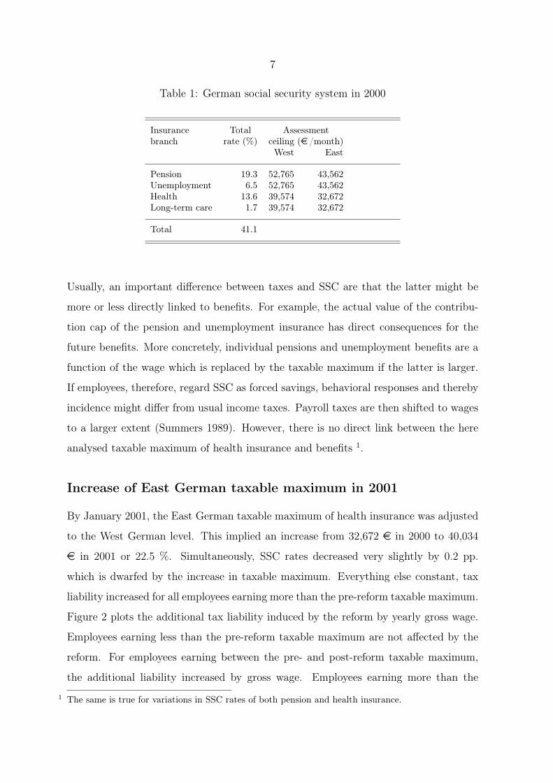
Table 1: German social security system in 2000

Insurance Total Assessmentbranch rate (%) ceiling (e /month)

West East

Pension 19.3 52,765 43,562Unemployment 6.5 52,765 43,562Health 13.6 39,574 32,672Long-term care 1.7 39,574 32,672

Total 41.1

Usually, an important difference between taxes and SSC are that the latter might be

more or less directly linked to benefits. For example, the actual value of the contribu-

tion cap of the pension and unemployment insurance has direct consequences for the

future benefits. More concretely, individual pensions and unemployment benefits are a

function of the wage which is replaced by the taxable maximum if the latter is larger.

If employees, therefore, regard SSC as forced savings, behavioral responses and thereby

incidence might differ from usual income taxes. Payroll taxes are then shifted to wages

to a larger extent (Summers 1989). However, there is no direct link between the here

analysed taxable maximum of health insurance and benefits 1.

Increase of East German taxable maximum in 2001

By January 2001, the East German taxable maximum of health insurance was adjusted

to the West German level. This implied an increase from 32,672 e in 2000 to 40,034

e in 2001 or 22.5 %. Simultaneously, SSC rates decreased very slightly by 0.2 pp.

which is dwarfed by the increase in taxable maximum. Everything else constant, tax

liability increased for all employees earning more than the pre-reform taxable maximum.

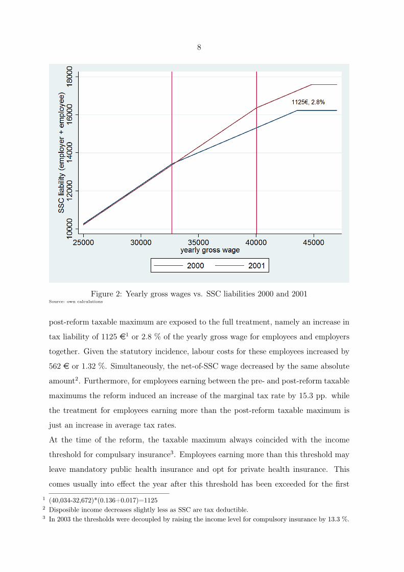
Figure 2 plots the additional tax liability induced by the reform by yearly gross wage.

Employees earning less than the pre-reform taxable maximum are not affected by the

reform. For employees earning between the pre- and post-reform taxable maximum,

the additional liability increased by gross wage. Employees earning more than the

1 The same is true for variations in SSC rates of both pension and health insurance.

8

Figure 2: Yearly gross wages vs. SSC liabilities 2000 and 2001Source: own calculations

post-reform taxable maximum are exposed to the full treatment, namely an increase in

tax liability of 1125 e1 or 2.8 % of the yearly gross wage for employees and employers

together. Given the statutory incidence, labour costs for these employees increased by

562 e or 1.32 %. Simultaneously, the net-of-SSC wage decreased by the same absolute

amount2. Furthermore, for employees earning between the pre- and post-reform taxable

maximums the reform induced an increase of the marginal tax rate by 15.3 pp. while

the treatment for employees earning more than the post-reform taxable maximum is

just an increase in average tax rates.

At the time of the reform, the taxable maximum always coincided with the income

threshold for compulsary insurance3. Employees earning more than this threshold may

leave mandatory public health insurance and opt for private health insurance. This

comes usually into effect the year after this threshold has been exceeded for the first

1 (40,034-32,672)*(0.136+0.017)=11252 Disposible income decreases slightly less as SSC are tax deductible.3 In 2003 the thresholds were decoupled by raising the income level for compulsory insurance by 13.3 %.

9

time. Therefore, most treated employees were exempted from compulsary insurance and

could be privately insured before the reform. This complicates the analysis since the

actual treatment is not known exactly for privately insured employees. The employee’s

contribution rate does not depend on wage but on individual characteristics implying

that the taxable maximum and its increase is irrelevant. The employer has to pay an

obligatory contribution which amounts to 50 % of an employee’s contributions up to

an upper threshold which is equal to an employer’s contribution for an publicly insured

employee earning the taxable maximum. Thus, if contributions of the private health

insurance are high enough, the reform had a similar effect on employer’s contributions

as in the case of public health insurance.

Further, the income threshold for compulsary insurance in East Germany increased as

well resulting in sudden compulsary insurance for employees earning between the pre-

and post-reform taxable maximums. Although an exception rule allowed this group of

employees to apply for being permanently exempted from compulsary insurance, there

might be an incentive for employees to switch from private to public health insurance.

For the employee this might increased or decreased her share depending on the actual

rates. By contrast, the employer’s part increased definately. If the pre-reform taxable

maximum was reached before the reform it increased as much as if the employee had

been publicly insured all along. If not it increased even more.

With the data set used so far privately and publicly insured employees cannot be dif-

ferentiated. However, an alternative data set, the employment panel of the Institute

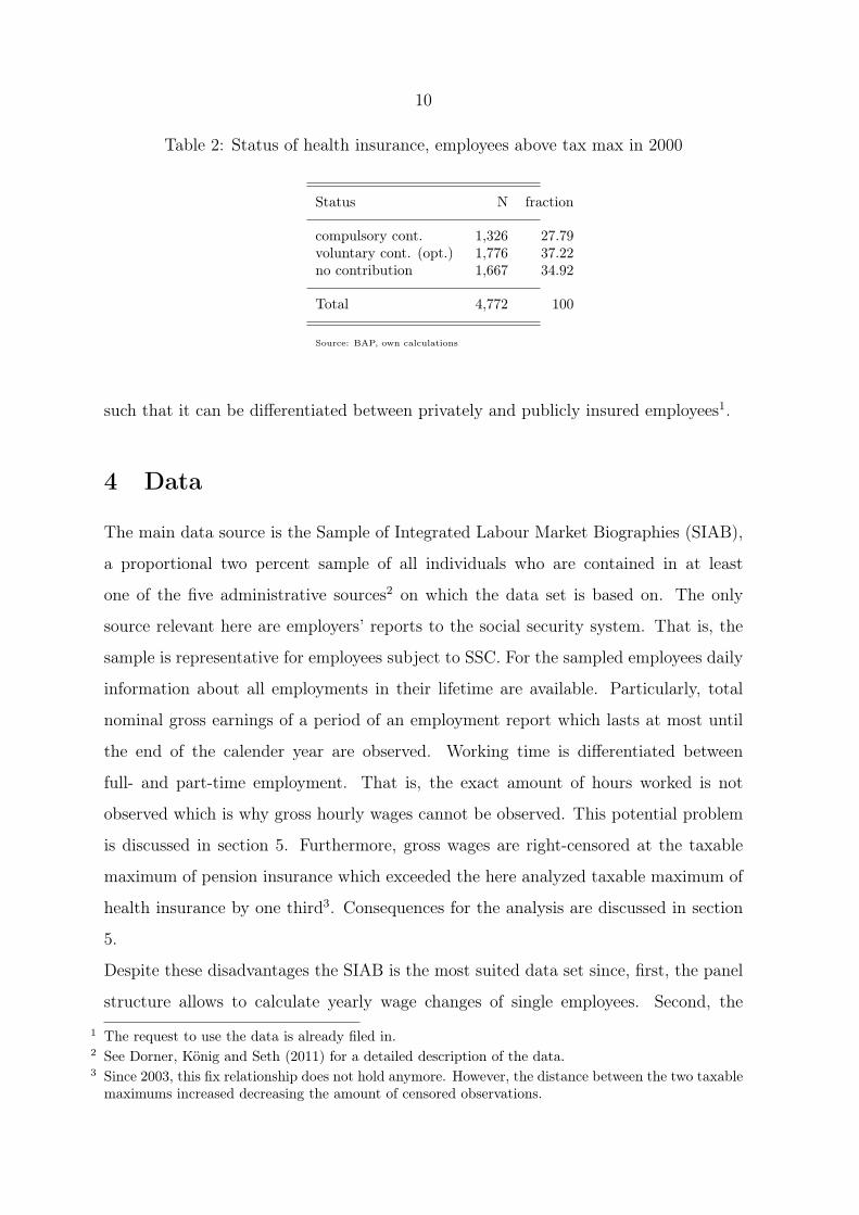
for Employment Research (IAB), includes the health insurance status. Table 2 shows

the distribution of this status within the treatment group. Roughly one third seems to

be privately insured ("no contribution"). Another one third are compulsory publicly

insured. They might have exceeded the threshold for the first time in 2000. Another

one third is voluntarily publicly insured. However, the latter declaration is voluntary

and it just includes voluntarily publicly insured employees whose employers transfer the

contributions directly. If that does not apply employees are coded as privately insured.

Hence, the amount of privately insured stated in table 2 (35 %) represents an upper

limit. Although 1/3 is not negligible, the problem seem to be smaller than one could

expect. Furthermore, in future the employment panel will be used for the whole analysis

10

Table 2: Status of health insurance, employees above tax max in 2000

Status N fraction

compulsory cont. 1,326 27.79voluntary cont. (opt.) 1,776 37.22no contribution 1,667 34.92

Total 4,772 100

Source: BAP, own calculations

such that it can be differentiated between privately and publicly insured employees1.

4 Data

The main data source is the Sample of Integrated Labour Market Biographies (SIAB),

a proportional two percent sample of all individuals who are contained in at least

one of the five administrative sources2 on which the data set is based on. The only

source relevant here are employers’ reports to the social security system. That is, the

sample is representative for employees subject to SSC. For the sampled employees daily

information about all employments in their lifetime are available. Particularly, total

nominal gross earnings of a period of an employment report which lasts at most until

the end of the calender year are observed. Working time is differentiated between

full- and part-time employment. That is, the exact amount of hours worked is not

observed which is why gross hourly wages cannot be observed. This potential problem

is discussed in section 5. Furthermore, gross wages are right-censored at the taxable

maximum of pension insurance which exceeded the here analyzed taxable maximum of

health insurance by one third3. Consequences for the analysis are discussed in section

5.

Despite these disadvantages the SIAB is the most suited data set since, first, the panel

structure allows to calculate yearly wage changes of single employees. Second, the

1 The request to use the data is already filed in.2 See Dorner, König and Seth (2011) for a detailed description of the data.3 Since 2003, this fix relationship does not hold anymore. However, the distance between the two taxablemaximums increased decreasing the amount of censored observations.

11

information about wages is very accurate due to the administrative character of the

data. Third, the sample size is comparatively large such that enough East German

employees are contained who earn between the taxable maximums of health and pension

insurance. And fourth, most factors important for wage dynamics are observed. On

individual level this includes particularly age, sex, occupation and education. Further,

experience and tenure can be derived due to the panel structure. On firm level, industry

sector1, size and wage structure are especially noteworthy. Furthermore, district of

workplace is included which allows for assigning a regional unemployment rate. Other

possible datasets lack in either exact wage information (German microcensus), panel

structure (FAST) or sample size (SOEP).

The sample is restricted in the following way. Only full-time employments are included

because they typically have smaller labour supply elasticities. In addition it is unlikely

for part-time workers to earn more than the taxable maximum anyway. Spells with

daily gross earnings below three euros or which last less than 14 days are assumed to

be measurement errors and dropped2. Employment reports handed in due to "miscel-

laneous reasons" are dropped as they comprise among others one-time payments which

do not represent a true employment spell3. Firm and job position changes are dropped

as well as employments which do not last the whole year. If an individual has two

parallel employment spells, the plausibility is checked. Two full-time employments are

assumed to be implausible as well as two employments in the same firm. In these

cases the employment with less earnings is assumed to be a measurement error and

dropped. Possible plausible combinations are two part-time employments or one full-

time emploment and a part-time employment as a side job. As we restrict the sample

to full-time employees, the first combination is dropped anyway. However, a possible

side job is used to assess if an employee earns more than the taxable maximum since

all labour earnings together are relevant. As the education variable is not necessary

for the administrative process, the quality is not as good as of most other variables

1 Aggregated into 16 groups.2 The actual threshold hardly influences the results as this study is mainly concerned with high earningemployees.

3 Usually such special payments are handed in with the usual employment reports; a specific report isjust used in special cases. In the weakly anonymized version of the data set one-time payments can beisolated exactly making it possible to treat them as the authorities do by adding them to the normalwage in the same period. This will be implemented.

12

(Dorner et al. 2011). Therefore, it is improved by an imputation procedure proposed

by Fitzenberger, Osikominu and Völter (2006)1. Moreover, the data is restricted to the

years 1994 to 2007.

5 Methodology

In order to isolate a causal effect of the reform on gross wages a difference-in-differences

approach is used. Due to potential downward rigiditiy of nominal wages, existing con-

tracts might mainly be affected by a change in wage dynamics. Therefore, yearly

changes in gross wages are used as outcome variable. Following Lang (2003), the wage

change between 2000 and 2001 is compared to wage changes of pairs of years which do

not feature a significant change in tax liability.

The Treatment Group

An issue is how to define the treatment group, that is how to identify employees which

are actually affected by the reform. Theoretically, all employees who would have earned

more than the pre-reform taxable maximum in 2001 in the absence of the reform are

directly affected. As this counterfactual outcome cannot be observed, there are two

alternative approaches to approximate the treatment group (Lang 2003).

First, it can be defined as employees earning more than the pre-reform taxable maximum

in 2000. By doing this, employees who would have earned less than the pre-reform

maximum in 2001 anyway are misclassified as they are not affected by the reform.

Similarly, employees who cross the taxable maximum in the reform year are classified

as not affected although they are. While employees of the latter group can be identified,

employees of the first group might pose a problem. Second, employees earning more

than the pre-reform taxable maximum in 2001 could serve as the treatment group.

Here, employees whose earnings decrease below the maximum due to the reform are

omitted. However, a decrease of earnings below the pre-reform cap would most likely

be driven by labour supply reactions instead of a here relevant decrease in hourly wages

as the latter would imply shifting of more than 100 %. The probability of such strong

1 The first procedure proposed is used as it is shown to perform the best .

13

labour supply reactions are discussed in section 5. So far, just the latter approximation

is implemented.

Another issue is if all employees above the pre-reform taxable maximum should be used.

Lang (2003) for example just used employees above the post-reform taxable maximum

as treatment group while Liang et al. (2004) used all employees above the pre-reform

taxable maximum. The disadvantage of the latter approach is that some employees

are exposed to a change in both, marginal and average tax rates potentially inducing

income and substitution effects. Additionally, the concrete treatment is heterogenous

and depends on how much earnings would exceed the pre-reform taxable maximum in

the absence of the reform. However, the loss of sample size by dropping these employees

might be even more problematic, particularly because the censoring threshold is only

approximately 5000 e higher than the post-reform taxable maximum in 2001. Here,

both approaches are used.

The Control Group

Two groups of employees offer themselves as control groups in order to control for

economy wide shocks or (potentially) shocks on industry level. First, West German

employees are not affected by the reform as their taxable maximum increased only

slightly by 1.2 %. The main advantage of this group is that employees earning more

than the West German taxable maximum can be used such that the pre-reform status is

comparable to the treatment group with respect to the reduced marginal and average tax

rates. However, relative to the median wage1, the taxable maximum is much higher in

East Germany. In 2000 it corresponded to 160 % of the median wage while the respective

West German value was just 135 %. Thus, the West German group is considerably

different to their East German counterpart with respect to its position in the wage

distribution. Simultaneously, defining the groups based on that position in the wage

distribution is not feasible as the upper threshold would be in the censored range2.

1 With respect to the data set resulting after the modifications discussed in section 4.2 An alternative would be to use the absolute values of the East German taxable maximum to isolatecontrol observations such that they are for example exposed to the same income tax rates as the treatedobservations. The disadvantage is that control observations then are exposed to a high marginal taxrate in both points in time.

14

The second natural control group are East German employees earning less than the

taxable maximum. The reasoning here is that - in comparison to a West German

control group - it also controls for regional shocks. The obvious disadvantages are the

different position in the wage distribution and a high marginal tax rate before and after

the reform. Thus, examples when the trend in wage changes might differ include for

example rising income inequality or reversion to the mean. A parameter to vary is the

lower earnings threshold. The choice represents a trade-off between comparability and

sample size. So far, it is chosen such that the sample size of treatment and control group

is roughly equal. Control observations, thus, feature yearly gross earnings between

27924 e and 32671 e. The validity of these two potential controls groups are discussed

in section 6.

Econometric Model

The following regression equation is estimated by OLS:

∆Yist = αs + γt + βDst + δXist + εist (1)

The outcome variable ∆Yist states the yearly log wage change of individual i in group s

in year t, αs are fixed effects for treatment and control group, γt are year fixed effects1,

Dst is the policy dummy which is one for observations in the treatment group in 2001,

Xist are potentially time-varying covariates on the individual, firm or regional level and

εist is an individual error term. The relevant coefficient is β which measures the part

of the difference in wage changes between treatment and control group in 2001, which

cannot be explained by the respective differences in other years (conditional on Xist).

Complications

Right-censoring of Wages

A complication is the right-censoring of wages in the data set at the taxable maximum

of the pension insurance as wage changes of censored observations are underreported.

1 Years 1995 to 2007 are included where the outcome variable in for example 1995 states the wage changebetween 1994 and 1995

15

If an employee earns below the taxable maximum only in the first (second) period

the wage decrease (increase) is underestimated. I solve this problem by imitating this

censoring for the control group. Thereby, the upper threshold of the control group is

treated as the counterpart of the taxable maximum. Observations with earnings above

a threshold in the second period do not belong to the respective group since the second

period is relevant for group allocation. Hence, treated observations which are censored

in the second period are dropped. Treated observations which are censored in the first

period but not in the second are counterparts to control observations which feature

earnings above the upper threshold in the first period and below in the second period.

In order to prevent underestimation, these observations are dropped for both, treatment

group and control group.

Other Reforms

A potential confounding factor for analyzing the increase of the taxable maximum in

2001 is the third step of a major tax reform in the same year. In November 1998, the

government published a draft of the tax reform whose three steps should have been

introduced in 1999, 2000 and 2002. Every step involved, among others, an increase

in the basic tax allowance and decreases of the tax rates. Thereby, the tax allowance

increased gradually by approximately 14 % from about 13,000 German Marks to about

14,000. The starting (highest) tax rate decreased overall from 25.9 to 19.9 % (53 to 48.5

%). In December 1998, the first step was decided upon by law. The second and third

step followed in March 1999. In July 2000, it was decided that the third step, originally

planned for 2002, will be introduced already by January of 2001. That is, simultaneous

to the reform analyzed in this article, the starting income tax rate decreased from 22.9

% to 19.9 %, the highest income tax rate from 51 % to 48.5 % and the basic tax

allowance increased from 13,500 German Marks to 14,000. Thus, the tax reform had

the potential to partly counteract the increase of the taxable maximum. Some points

should be noted here to alleviate the problem. First, by contrast to SSC, income taxes

are soley paid by employees. Depending on how important the formal organization is for

economic incidence, the tax reform might or might not have the potential to confound

the analysis. Second, as the tax reform potentially partly reverses the effects of the

16

analysed reform, the estimated effects not adjusted for the tax reform, are if anything

underestimated. Third and most important, while the tax reform decreased the income

tax similarly for the whole wage distribution and both German regions, the increase

of the taxable maximum just applied for East German employees earning above the

taxable maximum. Hence, both possible control groups are similarly affected by the

tax reform and should therefore control for its impact.

Labour supply effects

As already mentioned actual working time is not observed apart from the discreet

differentiation between part-time and full-time which is why hourly wages cannot be

calculated. Thus, an observed change in gross wages might be driven by a change

in hourly wages or by a change in actually hours worked. As this paper is about

incidence, the latter represents a source of bias. Furthermore, strong labour supply

reactions might be problematic if employees are assigned to the treatment group based

on earnings in 2001. Employees might adjust their labour supply in response to the

increase in marginal tax rate as leisure becomes relatively more attractiv (substitution

effect) or in response to the increase in average tax rate because the previous income

can just be realized by working more (income effect).

What might attentuate the problem is the finding of some studies that labour supply

elasticities of well earning, full-time employees are relatively small. For example, Al-

varedo and Saez (2007) and Saez (2010) do not find any labour supply reactions to the

existence of the taxable maximum in Spain and the US. By means of a classic labour

supply model, Saez (2010) predicts that a concave kink in the budget set, generated

by the drop in the marginal tax rate at the taxable maximum, leads to a gap in the

distribution1. According to the model, the dimension of the gap is directly linked to the

labour supply elasticity with respect to the net-of-tax rate. His reasoning is as follows:

The maximization of an iso-elastic utility function results in z = n(1− t)e with n being

a skill index, t the marginal tax rate, z gross earnings and e the elasticity of earnings

with respect to one minus the tax rate. If there is no tax, gross wages will equal the skill

1 As SSC are also paid by employers, their hiring behaviour might have similar consequences as discussedin Chetty, Friedman, Olsen and Pistaferri (2009).

17

index which is why n can be interpreted as potential earnings which are depressed by

a tax. The cumulative distribution function of earnings given a constant marginal tax

rate t0 is H0(z) = Pr(n(1− t0)e ≤ z) = F (z/(1− t0)

e) with F (n) being the cumulative

density function of the skill level. Thus, h0(z) = f( z(1−t0)e

)/(1 − t0)e. If now a taxable

maximum is introduced at z*, earnings above z* are not distorted anymore, implying

z = n. Hence, the new density above the cap is h(z) = f(n) = h0(z(1− t0)e) ∗ (1− t0)

e,

while below the cap it does not change, implying h(z) = h0(z). Thus, the limits of both

sides of the cap are:

h(z) =

h0(z∗) if z < z∗

h0(z∗(1 − t0)

e) ∗ (1 − t0)e if z ≥ z∗

(2)

That is, if potential earnings are above z∗, they will be realized. But if potential earnings

are below z∗, they are further distorted because employees choose to work less in order

to locate farther away from the taxable maximum. This leaves a gap left of the taxable

maximum1. Due to that gap the left value of h(z) will rather be h0(z∗(1 − t0)e) which

is the first value which can occur. On the right side of the gap, the density is decreased

by the factor of (1 − t0)e as the parts of the incomes are not exposed to redistribution,

leaving the density of earnings less concentrated and therefore lower at a given earnings

level. Figure [to be included] shows the East German wage distribution around the

taxable maximum of health insurance generated with the SIAB. The distribution seems

to be quite smooth around the taxable maximum implying that the predicted features

are not present. Given the underlying model is a good approximation, this suggests

that the labour supply elasiticity of employees above the taxable maximum is close to

zero. This is consistent with the above mentioned findings of Alvaredo and Saez (2007)

and Saez (2010) for Spanish and US data.

1 Given that employees cannot adjust their earnings perfectly, there rather will be a trough.

18

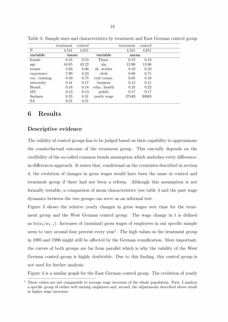
Table 3: Sample sizes and characteristics by treatment and East German control grouptreatment control treatment control

N 4,541 4,651 4,541 4,651variable mean variable meanfemale 0.45 0.54 Thuer. 0.15 0.18age 44.65 43.22 alq 13.90 13.86tenure 5.63 6.06 sk. worker 0.10 0.23experience 7.90 8.23 clerk 0.86 0.71voc. training 0.50 0.75 traf/comm. 0.05 0.10university 0.41 0.17 business 0.15 0.11Brand. 0.16 0.18 educ./health 0.25 0.22MV 0.13 0.13 public 0.17 0.17Sachsen 0.35 0.31 yearly wage 37449 30363SA 0.21 0.21

6 Results

Descriptive evidence

The validity of control groups has to be judged based on their capability to approximate

the counterfactual outcome of the treatment group. This curcially depends on the

credibility of the so-called common trends assumption which underlies every difference-

in-differences approach. It states that, conditional on the covariates described in section

4, the evolution of changes in gross wages would have been the same in control and

treatment group if there had not been a reform. Although this assumption is not

formally testable, a comparison of mean characteristics (see table 3 and the past wage

dynamics between the two groups can serve as an informal test.

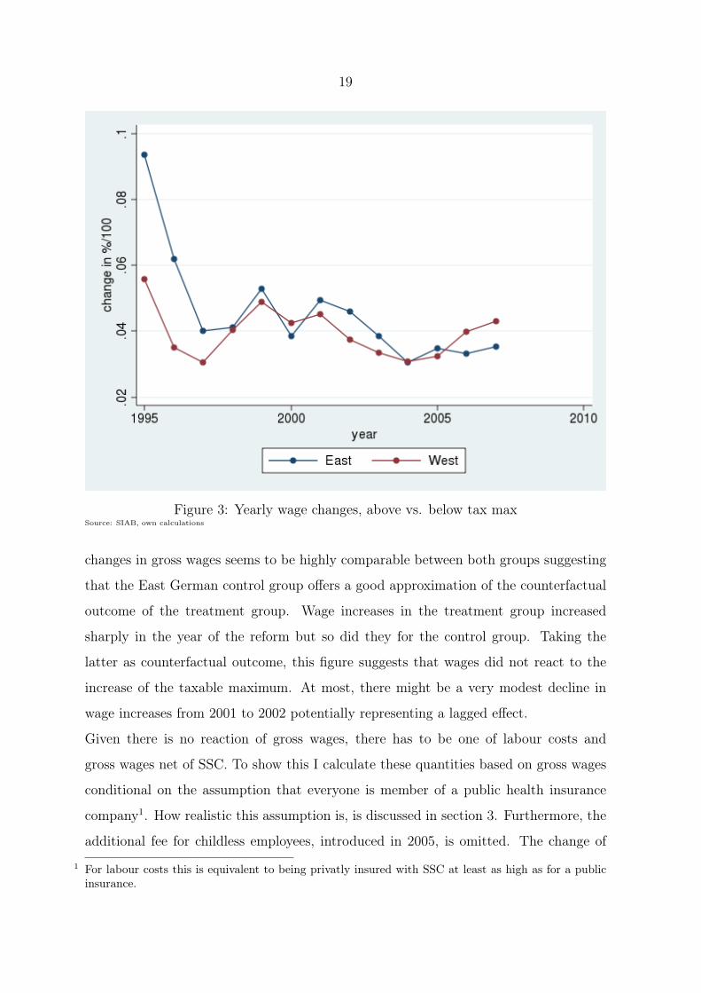
Figure 3 shows the relative yearly changes in gross wages over time for the treat-

ment group and the West German control group. The wage change in t is defined

as ln(wt/wt−1). Increases of (nominal) gross wages of employees in our specific sample

seem to vary around four percent every year1. The high values in the treatment group

in 1995 and 1996 might still be affected by the German reunification. More important,

the curves of both groups are far from parallel which is why the validity of the West

German control group is highly doubtable. Due to this finding, this control group is

not used for further analysis.

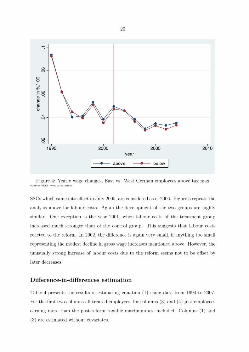
Figure 4 is a similar graph for the East German control group. The evolution of yearly

1 These values are not comparable to average wage increases of the whole pupulation. First, I analyzea specific group of rather well earning employees and, second, the adjustments described above resultin higher wage increases.

19

Figure 3: Yearly wage changes, above vs. below tax maxSource: SIAB, own calculations

changes in gross wages seems to be highly comparable between both groups suggesting

that the East German control group offers a good approximation of the counterfactual

outcome of the treatment group. Wage increases in the treatment group increased

sharply in the year of the reform but so did they for the control group. Taking the

latter as counterfactual outcome, this figure suggests that wages did not react to the

increase of the taxable maximum. At most, there might be a very modest decline in

wage increases from 2001 to 2002 potentially representing a lagged effect.

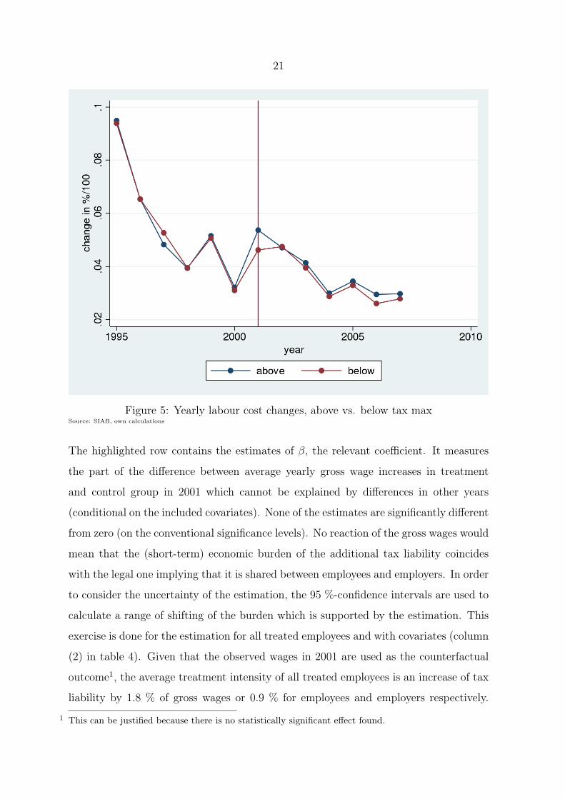
Given there is no reaction of gross wages, there has to be one of labour costs and

gross wages net of SSC. To show this I calculate these quantities based on gross wages

conditional on the assumption that everyone is member of a public health insurance

company1. How realistic this assumption is, is discussed in section 3. Furthermore, the

additional fee for childless employees, introduced in 2005, is omitted. The change of

1 For labour costs this is equivalent to being privatly insured with SSC at least as high as for a publicinsurance.

20

Figure 4: Yearly wage changes, East vs. West German employees above tax maxSource: SIAB, own calculations

SSCs which came into effect in July 2005, are considered as of 2006. Figure 5 repeats the

analysis above for labour costs. Again the development of the two groups are highly

similar. One exception is the year 2001, when labour costs of the treatment group

increased much stronger than of the control group. This suggests that labour costs

reacted to the reform. In 2002, the difference is again very small, if anything too small

representing the modest decline in gross wage increases mentioned above. However, the

unusually strong increase of labour costs due to the reform seems not to be offset by

later decreases.

Difference-in-differences estimation

Table 4 presents the results of estimating equation (1) using data from 1994 to 2007.

For the first two columns all treated employees, for columns (3) and (4) just employees

earning more than the post-reform taxable maximum are included. Columns (1) and

(3) are estimated without covariates.

21

Figure 5: Yearly labour cost changes, above vs. below tax maxSource: SIAB, own calculations

The highlighted row contains the estimates of β, the relevant coefficient. It measures

the part of the difference between average yearly gross wage increases in treatment

and control group in 2001 which cannot be explained by differences in other years

(conditional on the included covariates). None of the estimates are significantly different

from zero (on the conventional significance levels). No reaction of the gross wages would

mean that the (short-term) economic burden of the additional tax liability coincides

with the legal one implying that it is shared between employees and employers. In order

to consider the uncertainty of the estimation, the 95 %-confidence intervals are used to

calculate a range of shifting of the burden which is supported by the estimation. This

exercise is done for the estimation for all treated employees and with covariates (column

(2) in table 4). Given that the observed wages in 2001 are used as the counterfactual

outcome1, the average treatment intensity of all treated employees is an increase of tax

liability by 1.8 % of gross wages or 0.9 % for employees and employers respectively.

1 This can be justified because there is no statistically significant effect found.

22

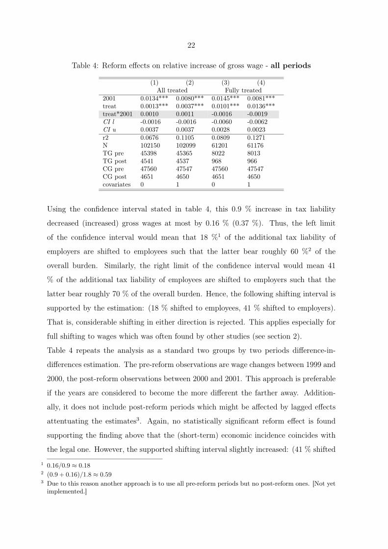
Table 4: Reform effects on relative increase of gross wage - all periods

(1) (2) (3) (4)All treated Fully treated

2001 0.0134*** 0.0080*** 0.0145*** 0.0081***treat 0.0013*** 0.0037*** 0.0101*** 0.0136***treat*2001 0.0010 0.0011 -0.0016 -0.0019CI l -0.0016 -0.0016 -0.0060 -0.0062CI u 0.0037 0.0037 0.0028 0.0023r2 0.0676 0.1105 0.0809 0.1271N 102150 102099 61201 61176TG pre 45398 45365 8022 8013TG post 4541 4537 968 966CG pre 47560 47547 47560 47547CG post 4651 4650 4651 4650covariates 0 1 0 1

Using the confidence interval stated in table 4, this 0.9 % increase in tax liability

decreased (increased) gross wages at most by 0.16 % (0.37 %). Thus, the left limit

of the confidence interval would mean that 18 %1 of the additional tax liability of

employers are shifted to employees such that the latter bear roughly 60 %2 of the

overall burden. Similarly, the right limit of the confidence interval would mean 41

% of the additional tax liability of employees are shifted to employers such that the

latter bear roughly 70 % of the overall burden. Hence, the following shifting interval is

supported by the estimation: (18 % shifted to employees, 41 % shifted to employers).

That is, considerable shifting in either direction is rejected. This applies especially for

full shifting to wages which was often found by other studies (see section 2).

Table 4 repeats the analysis as a standard two groups by two periods difference-in-

differences estimation. The pre-reform observations are wage changes between 1999 and

2000, the post-reform observations between 2000 and 2001. This approach is preferable

if the years are considered to become the more different the farther away. Addition-

ally, it does not include post-reform periods which might be affected by lagged effects

attentuating the estimates3. Again, no statistically significant reform effect is found

supporting the finding above that the (short-term) economic incidence coincides with

the legal one. However, the supported shifting interval slightly increased: (41 % shifted

1 0.16/0.9 ≈ 0.182 (0.9 + 0.16)/1.8 ≈ 0.593 Due to this reason another approach is to use all pre-reform periods but no post-reform ones. [Not yetimplemented.]

23

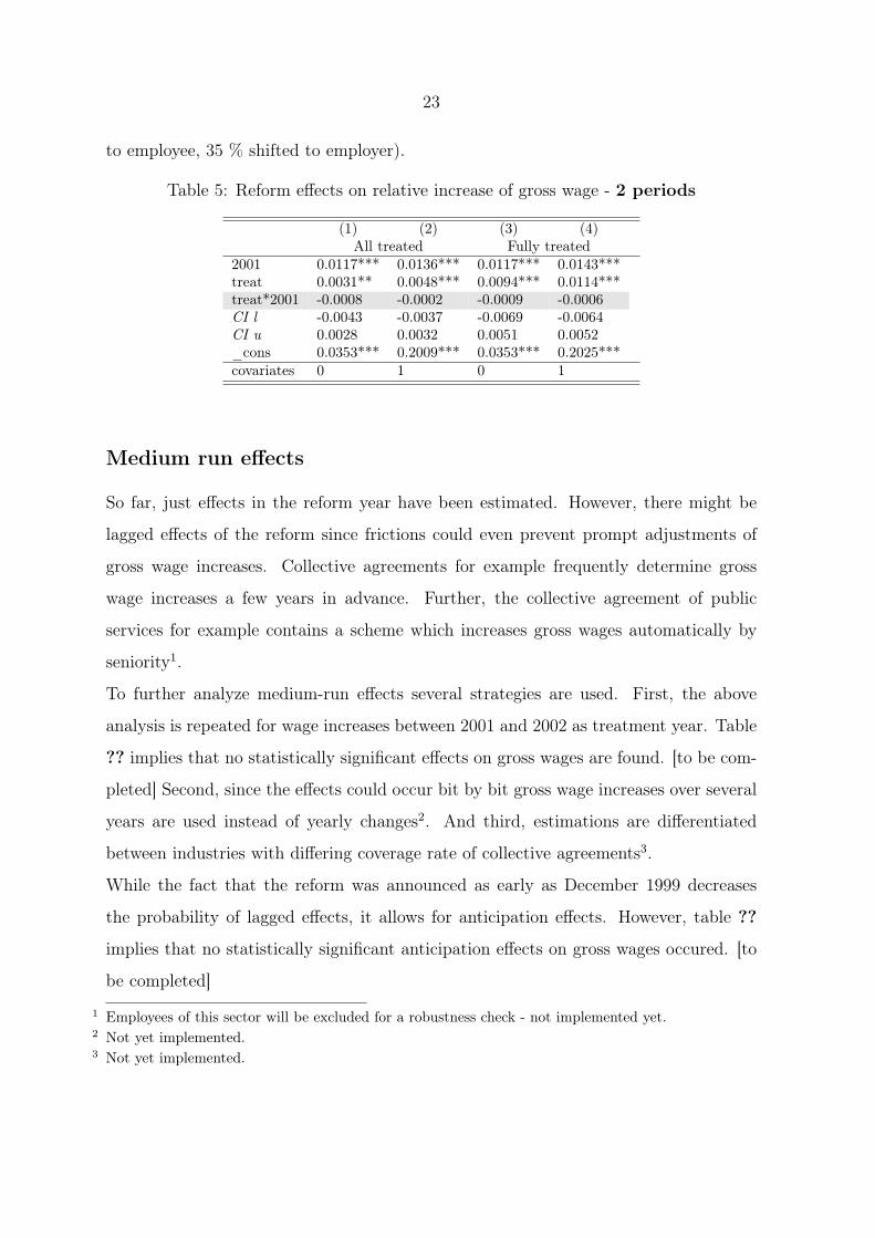
to employee, 35 % shifted to employer).

Table 5: Reform effects on relative increase of gross wage - 2 periods

(1) (2) (3) (4)All treated Fully treated

2001 0.0117*** 0.0136*** 0.0117*** 0.0143***treat 0.0031** 0.0048*** 0.0094*** 0.0114***treat*2001 -0.0008 -0.0002 -0.0009 -0.0006CI l -0.0043 -0.0037 -0.0069 -0.0064CI u 0.0028 0.0032 0.0051 0.0052_cons 0.0353*** 0.2009*** 0.0353*** 0.2025***covariates 0 1 0 1

Medium run effects

So far, just effects in the reform year have been estimated. However, there might be

lagged effects of the reform since frictions could even prevent prompt adjustments of

gross wage increases. Collective agreements for example frequently determine gross

wage increases a few years in advance. Further, the collective agreement of public

services for example contains a scheme which increases gross wages automatically by

seniority1.

To further analyze medium-run effects several strategies are used. First, the above

analysis is repeated for wage increases between 2001 and 2002 as treatment year. Table

?? implies that no statistically significant effects on gross wages are found. [to be com-

pleted] Second, since the effects could occur bit by bit gross wage increases over several

years are used instead of yearly changes2. And third, estimations are differentiated

between industries with differing coverage rate of collective agreements3.

While the fact that the reform was announced as early as December 1999 decreases

the probability of lagged effects, it allows for anticipation effects. However, table ??

implies that no statistically significant anticipation effects on gross wages occured. [to

be completed]

1 Employees of this sector will be excluded for a robustness check - not implemented yet.2 Not yet implemented.3 Not yet implemented.

24

Table 6: Reform effects on relative increase of gross wage - 2000 and 2002

(1) (2) (3) (4)All treated Fully treated

2000*treat 0.0019 0.0019 -0.0006 -0.0010CI l -0.0007 -0.0007 -0.0052 -0.0054CI u 0.0045 0.0045 0.0040 0.00352002*treat -0.0015 -0.0020 0.0024 0.0013CI l -0.0044 -0.0049 -0.0024 -0.0035CI u 0.0014 0.0009 0.0073 0.0060

7 Conclusion

This paper uses a test for the incidence of SSC solely based on yearly gross wage in-

creases and applies it to the increase of the East German taxable maximum of health

insurance. It is shown that East German employees earning somewhat less than the

taxable maximum is a valid control group. By conducting difference-in-differences es-

timations I find that neither employers nor employees seem to be able to shift more

than 50 % of the additional tax liability to the respective other. Particularly, it rejects

the frequently used assumption that the burden is usually shifted completely to wages.

Rather, it seems that employers and employees seem to share the burden equally. This

might be either due to a specific constellation of preferences or, more probably, the

formal split of SSC plays a strong role for their incidence. The latter implies that the

invariance of incidence proposition does not seem to hold for German SSC.

[to be completed]

25

References

Alvaredo, Facundo and Emmanuel Saez, “The Effects of Payroll Taxes on Earn-

ings: Evidence from Spanish Administrative Data,” Technical Report 2007.

Bauer, Thomas and Regina T. Riphahn, “Employment Effects of Payroll Taxes

- An Empirical Test for Germany,” IZA Discussion Papers 11, Institute for the

Study of Labor (IZA) June 1998.

Bennmarker, Helge, Erik Mellander, and Björn Öckert, “Do regional payroll

tax reductions boost employment?,” Labour Economics, 2009, 16 (5), 480 – 489.

Bohm, Peter and Hans Lind, “Policy evaluation quality: A quasi-experimental

study of regional employment subsidies in Sweden,” Regional Science and Urban

Economics, 1993, 23 (1), 51 – 65.

Brittain, John A, “The Incidence of Social Security Payroll Taxes,” American Eco-

nomic Review, March 1971, 61 (1), 110–25.

Chetty, Raj, John N. Friedman, Tore Olsen, and Luigi Pistaferri, “Adjustment

Costs, Firm Responses, and Micro vs. Macro Labor Supply Elasticities: Evidence

from Danish Tax Records,” NBER Working Papers 15617, National Bureau of

Economic Research, Inc December 2009.

Daveri, Francesco and Guido Tabellini, “Unemployment, growth and taxation in

industrial countries,” Economic Policy, 04 2000, 15 (30), 47–104.

Dorner, Matthias, Marion König, and Stefan Seth, “Stichprobe der Integri-

erten Arbeitsmarktbiografien. Regionalfile 1975-2008 (SIAB-R 7508),” FDZ Daten-

report. Documentation on Labour Market Data 201107, Institut für Arbeitsmarkt-

und Berufsforschung (IAB), Nürnberg [Institute for Employment Research, Nurem-

berg, Germany] October 2011.

Fatima, Freeha, “The Incidence of Payroll Taxes in Pakistan: Evidence from a Firm-

size-contingent Policy Change,” Technical Report 2012.

26

Fitzenberger, Bernd, Aderonke Osikominu, and Robert Völter, “Imputation

Rules to Improve the Education Variable in the IAB Employment Subsample,”

Schmollers Jahrbuch : Journal of Applied Social Science Studies / Zeitschrift für

Wirtschafts- und Sozialwissenschaften, 2006, 126 (3), 405–436.

Gruber, Jonathan, “The Incidence of Payroll Taxation: Evidence from Chile,” Jour-

nal of Labor Economics, July 1997, 15 (3), S72–101.

Hamermesh, Daniel S., “New Estimates of the Incidence of the Payroll Tax,” South-

ern Economic Journal, 1979, 45 (4), pp. 1208–1219.

Holmlund, Bertil, “Payroll Taxes and Wage Inflation: The Swedish Experience,”

Scandinavian Journal of Economics, 1983, 85 (1), 1–15.

Johansen, F. and T.J. Klette, “Wage and Employment Effects of Payroll Taxes

and Investment Subsidies,” Memorandum 27/1998, Oslo University, Department

of Economics 1998.

Korkeamäki, Ossi and Roope Uusitalo, “Employment and wage effects of a payroll-

tax cut—evidence from a regional experiment,” International Tax and Public Fi-

nance, December 2009, 16 (6), 753–772.

Lang, Kevin, “The Effect of the Payroll Tax on Earnings: A Test of Competing

Models of Wage Determination,” NBER Working Papers 9537, National Bureau

of Economic Research, Inc March 2003.

Liang, Xiaoli, Jeffrey Kubik, and Gary Engelhardt, “The Incidence of the Social

Security Payroll Tax: Evidence from the 1977 Amendments to the Social Security

Act,” Technical Report 2004.

Neubig, Thomas, “The Social Security Payroll Tax Effect on Wage Growth,” Pro-

ceedings of the National Tax Association, 1981, pp. 196–201.

OECD, “OECD Employment Output: EMPLOYER VERSUS EMPLOYEE TAXA-

TION: THE IMPACT ON EMPLOYMENT,” Technical Report, OECD 1990.

27

Saez, Emmanuel, “Do Taxpayers Bunch at Kink Points?,” American Economic Jour-

nal: Economic Policy, August 2010, 2 (3), 180–212.

Skedinger, Per, “Effects of Payroll Tax Cuts for Young Workers: Evidence from

Swedish Retail,” Technical Report, Research Institute of Industrial Economics

2012.

Summers, Lawrence H, “Some Simple Economics of Mandated Benefits,” American

Economic Review, May 1989, 79 (2), 177–83.

Vroman, Wayne, “Employer Payroll Tax Incidence: Empirical Tests with Cross-

Country Data,” Public Finance = Finances publiques, 1974, 29 (2), 184–200.