Embed Size (px)
Citation preview
The Impact of the Macroeconomic Environment
on Microfinance Sustainability: Measuring the Effects of Inflation, Interest Rates, Unemployment and
Per Capita GDP on MFI Profitability and Repayment Rates
By: Jordan van Rijn
Master of Pacific and International Affairs Candidate, 2008
Graduate School of International and Pacific Studies
University of California, San Diego
Abstract:
Microfinance has recently gained prestige as an effective way of combating poverty in the
developing world. Recently, attention has focused on making microfinance a sustainable endeavor,
thereby enabling practitioners to reach millions of new clients without having to rely on subsidies.
However, some argue that the volatile macro-economic climate in developing countries precludes
this objective. This paper uses a Random Effects regression model to examine the impact of the
macro-economic climate (using inflation, unemployment rates, interest rates and per-capita GDP
as causal variables) on MFI sustainability (measured by repayment rates and ROE). We find that
per-capita GDP is a highly significant determinant of MFI profitability. Particularly in high-income
developing nations, a higher average income appears conducive to greater MFI profits. However,
the macro-economic climate has no impact on repayment rates. Overall, it appears that—except
for the income effect— the macro-economic climate has little impact on MFI sustainability.
1
I. Introduction
Since the late 1970s and early 1980s, microfinance has expanded all across the developing
world, adapting and changing to each new culture and situation, and everywhere raising eyebrows
because of its amazing ability to combat poverty. It is estimated that microfinance institutions (MFIs)
currently reach 80 million families worldwide.1 Basically, the idea of microfinance is simple: provide
small loans—often less than $100US—and other financial services to people who ordinarily would be
left out of the banking sector because of “poor-credit worthiness” or lack of collateral. Despite its
simplicity, however, microfinance practitioners are currently grappling with an enormous challenge:
sustainability. How are MFIs to reach the millions of potential borrowers if they are constantly in need of
grants and donations to fund their operations? The Grameen Bank—arguably the most successful and
far-reaching MFI—has received millions in subsidies since its inception and continues to rely on outside
support.2 Indeed, sustainability has proven to be a difficult goal, especially when working in developing
countries where inflation and interest rates are often quite high, unemployment rates erratic and income
very low. Many argue that the volatile nature of developing countries makes financial investment a risky
business.3 Others, like most commercial banks, posit that low incomes and small loan sizes do not
allow high enough margins to cover the costs involved in operating MFIs.4 Yet, how important are
macro-economic indicators—like inflation and per-capita GDP—for microfinance sustainability? Clearly,
the answer to this question has major implications for the future expansion of the microfinance sector.
Hence, this paper analyzes the effects of macro-level economic indicators on two measures of
microfinance sustainability: return on equity (ROE) and repayment rates.
1 Japanonica, p. 1
2 Morduch & Armendáriz de Aghion, p. 235-6
3 For one example, see Ilan Goldfajn & Roberto Rigobon’s “Hard Currency and Financial Development.”
Department of Economics, PUC-Rio (Brazil). (Dec. 2000). 4 Yunus, p. 52
2
Several papers have already examined the impact of macro-economic indicators on financial
development and MFIs. Goldfajn and Rigobon (2000), for example, show that macro-economic
stability—determined by stable inflation and real interest rates—is crucial for development of the
financial sector. Similarly, Vander Weele and Markovich (2001) provide case studies of Opportunity
International’s experience in Russia and Bulgaria that illustrate the devastating effects of inflation and
hyperinflation on MFIs. On a somewhat different note, McGuire and Conroy (1998) have explored the
impact of the Asian Financial Crisis on the microfinance sector in Southeast Asia; they tentatively
conclude that countries with the greatest concentrations of poverty have been little affected by the
crisis.
To my knowledge, however, the most recent, comprehensive study of the impact of the macro-
economic environment on MFIs has been the study by Annabel Vanroose (2006) on the uneven
development of microfinance in Latin America. Vanroose uses regression analysis to test the impact of
various factors on microfinance outreach (defined as the percentage of the population served by
microfinance institutions in 2001). Using this as her dependent variable, she explores the impact of
various causal variables including inflation rate, GNI per capita, population density, literacy rate, aid per
capita, foreign assets per capita, industry value added and a dummy for whether the MFI is located in a
country with a special regulatory framework. Interestingly, Vanroose finds that microfinance is more
developed in economically instable countries, showing a positive correlation between inflation rates and
microfinance outreach (significant at the 5% level). She justifies this finding by arguing that higher
inflation renders people more familiar with the high interest rates common to MFIs. Vanroose did not
find that GNI per capita was a statistically significant determinant of microfinance outreach.
Although Vanroose’s efforts are laudable, her paper has a couple of major faults. The first is
that the data she uses is a cross-section of Latin American countries in 2001; clearly, data from only
one year will not enable her model to control for country-specific fixed effects or spurious correlation.
3
Furthermore, microfinance outreach is not necessarily the best proxy for understanding development of
the microfinance sector. Surely, international development organizations may specifically target
countries that are less economically stable because these also tend to be the countries with the highest
rates of poverty. Furthermore, some MFIs may put forth much more effort towards expansion than
others. Also, some countries may only have a few MFIs that are very profitable and sustainable, while
other countries may have a plethora of MFIs that are unprofitable and inefficient but are being
supported by foreign aid.
My analysis, then, uses panel data of 85 MFIs from 1999 to 2005 and uses repayment rates
and return on equity (ROE) as measures of MFI performance and sustainability. I hope to answer the
following questions: What is the impact of the macro-economic environment—measured by inflation,
interest rates, unemployment rates and per capita GDP—on MFI repayment rates and profitability?
Does this impact depend on the type of MFI, the region where it is located and whether the MFI is
regulated? What are the implications of these findings for organizations hoping to establish sustainable
MFIs?
II. Data
The microfinance-specific data I use is from The Mix Market (www.mixmarket.org). Although
there is data from over 900 MFIs available in the database, I only found 85 with the information I
needed to perform my analysis. My criterion for selecting MFIs was that they had to have continuous
data from years 1999-2005 including ROE, return on assets (ROA), number of borrowers, average loan
size, portfolio at risk, percentage of female borrowers and total assets. The macro-economic data is
from the online United Nations Statistics Division (http://unstats.un.org/unsd/default.htm) and includes
country-specific data of total unemployment for men and women, unemployment rates for men and
4
women, total unemployment rates, consumer price indices, per capita GDP and interest rates (banks’
prime lending). The data was analyzed using Stata.
I performed regressions with two main models, using the following dependent variables:
Table 1: Dependent Variables Dependent Variable (w/Stata names in parentheses)
Description
Return on Equity (ROE) Measure of profitability of MFI: Net Operating Income Less Taxes / Average Annual Equity
Portfolio at Risk (Risk) Measure of borrower repayment: Portfolio at Risk > 30 days / Gross Loan Portfolio
*Note: ROE, not ROA, was used as a proxy for profitability given the specific characteristics of MFIs. This is consistent with other similar research papers.5 Regardless, the two measures give similar results and are highly correlated (pwcorr=0.72).
For a complete list of independent variables, including my control variables and main causal
variables, see Table 2.
III. Empirical Methodology
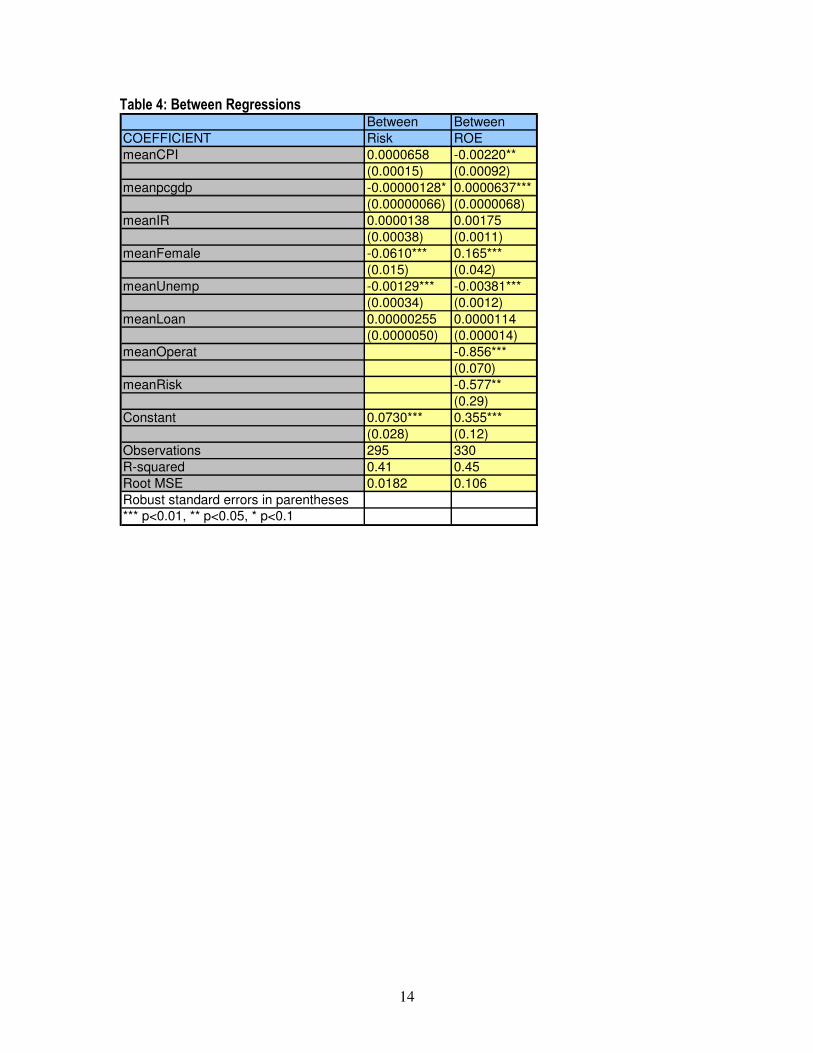
I began my analysis by running a “between estimator” and Pooled OLS regression for each of
the two models using “robust” standard errors and weighting by number of borrowers (see Tables 3 &
4). The between regressions seem to indicate that, in the cross-section, high Risk is usually
accompanied by low unemployment and more male borrowers. In the ROE model, high ROE is found
with high per-capita GDP, more female borrowers, less unemployment, few operating expenses and
low Risk. However, since the between estimator only measures cross-sectional variation and Pooled
OLS assumes that nothing differs across MFIs that is unobservable (an unlikely assumption), I decided
to move more towards “within” analysis.
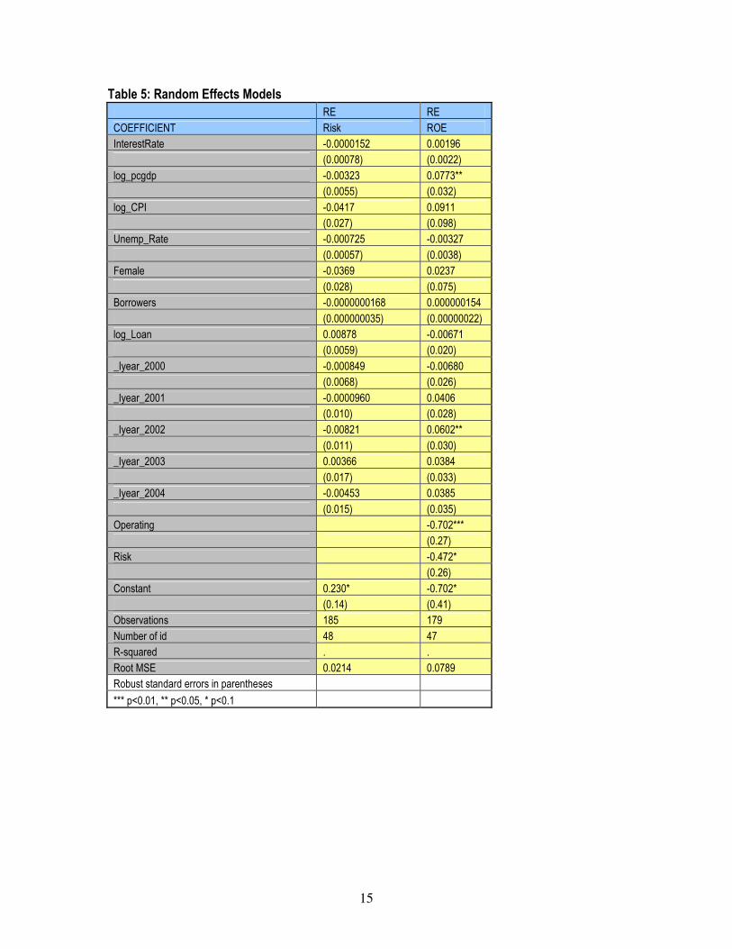
After logging CPI, pcgdp and Loan to account for large differences in proportions, I ran Fixed
Effects (FE) and Random Effects (RE) regressions for each model. This was followed by a Hausman
test to check whether the difference in FE and RE coefficients was systematic. In both models, the
5 For examples, see Japanoica’s “Microfinance for Profit” or Krauss and Walters “Can Microfinance Reduce
Portfolio Volatility.”
5
difference was not systematic. Therefore, I elected to use the RE model since it is both efficient and
unbiased. This model will partially demean the data to correct for the correlation between the time
variant and time invariant errors and then use Pooled OLS for the data that is not correlated (see Table
5 for regression outputs). Note: Because Stata does not allow use of weighting commands in an RE
model, I added Borrowers as a control variable to account for the different sizes of MFIs.
My two estimating equations are as follows:
1. Repayment Model:
� Risk = β0 + β1InterestRate + β2 log_pcgdp + β3log_CPI + β4Unemp_Rate +
� β5Female + β6log_loan + β7Borrowers + ∑δyear + αi uit
2. Profitability Model:
� ROE = β0 + β1InterestRate + β2 log_pcgdp + β3 Operating + β4log_CPI +
� β5Unemp_Rate + β6 Risk + β7Female + β8log_loan + β9Borrowers + ∑δyear + αi uit
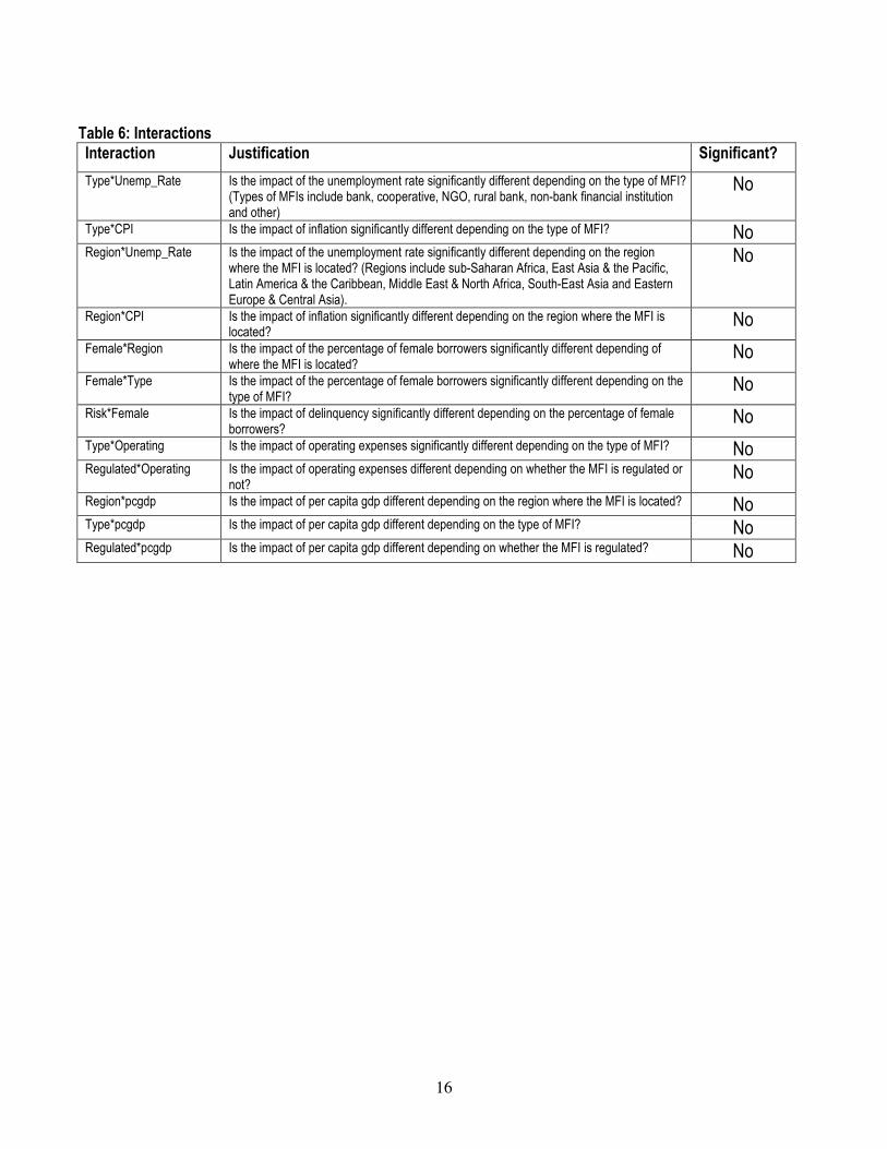
Interactions: None of the interactions I attempted proved to be statistically significant (see Table 6).
Therefore, I will retain the above models.
IV. Results
Interestingly, the Repayment Model shows no statistically significant independent variables.
This was the case even after attempting various interactions. It would appear, then, that none of the
macro-economic indicators have a significant impact on repayment rates. Also interesting is the fact
that Female—although clearly an endogenous variable—also showed no statistical significance. This
appears to counter the oft-cited argument that women make better borrowers than men.

6
In the Profitability Model, we find that operating expenses and per-capita GDP are statistically
significant determinants of ROE. The impact of operating expenses is not terribly surprising, since
having higher operating expenses is obviously going to decrease ROE (as the negative sign on the
coefficient indicates). The positive coefficient on per-capita GDP is a bit less mechanical. Some might
argue that higher incomes lead to a higher loan size which is shown to increase MFI profits;6 but the
Grameen Bank has amply demonstrated that MFIs in low-income nations can also be sustainable and
profitable, even while lending to the poorest of the poor.7
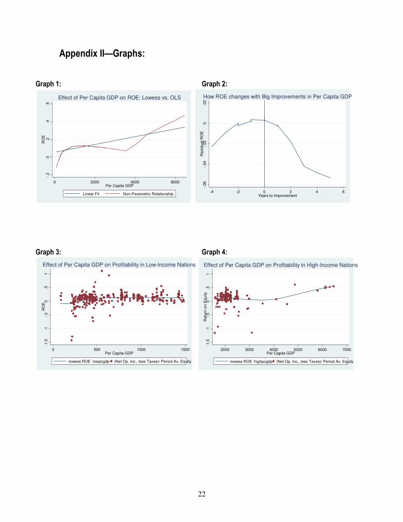
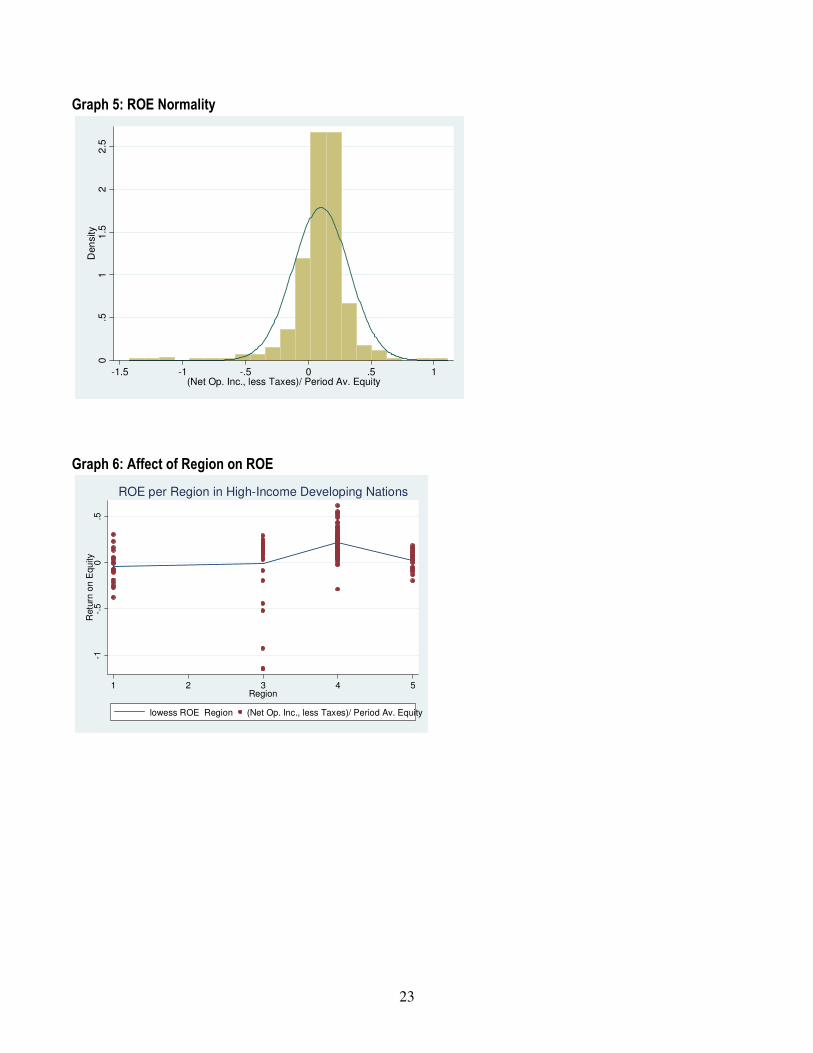
When comparing the OLS regression to a lowess non-parametric fit, it is obvious that the linear
regression does not provide a very accurate estimate of the impact of per-capita GDP on ROE (see
Graph 1). At times ROE appears to increase with GDP per-capita and at other times it appears to
decrease. Using the year that each country experienced its greatest improvement in per-capita GDP as
a proxy for a treatment, I attempted to analyze the effects of a big jump in per-capita GDP on ROE
(Graph 2). As you can see, ROE increases until directly after the treatment, when it sharply declines.
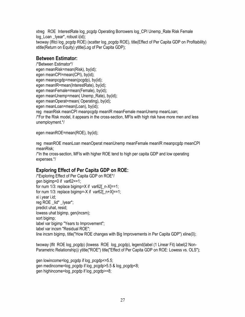
Based on Graph 1, I decided to create two new variables to further analyze the impact of per-
capita GDP on ROE: I created a lowincome variable for nations with a per-capita GDP of under
$1500US and a highincome variable for nations with a per-capita GDP of $1500US and higher. Now,
we can clearly see that per-capita GDP has no impact on low-income developing nations (see Graph
3), but it does have a highly significant impact in high-income developing nations (see Graph 4 and
Table 7). However, this result appears to be driven by one outlier, Banco Compartamos in Mexico,
where the per-capita GDP and ROE are among the highest (see Graph 4). Yet, when removing this
MFI from the regression, per-capita GDP is still statistically significant at the 90% level.
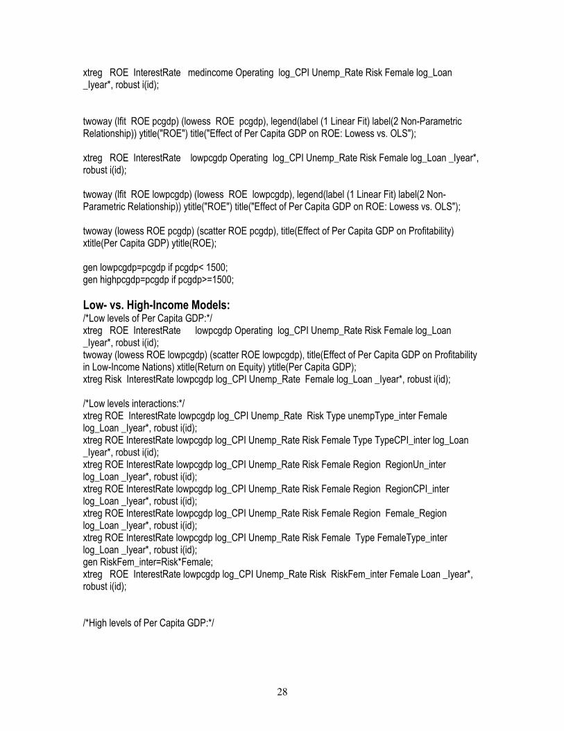
Another interesting outcome of splitting the data into low- and high-income developing country
models is that, when adding Region, we find that it is now highly significant in the high-income model.
6 Morduch & de Aghion, p. 263
7 For the story of the Grameen Bank, see Muhammad Yunus’ Banker to the Poor.
7
However, this impact appears to be specific to Latin America, where there is a huge jump in ROE
compared to other regions (see Graph 6).
V. Potential Problems
In this section I will discuss some of the potential problems with these models and whether this
limits my overall findings:
1. Data:
Firstly, it should be stated that the data used for these models is not ideal. Although it is panel
data—a definite advantage over cross-sectional data—the final models only have 185 and 179
observations, respectively; this does not provide an optimal number of degrees of freedom and the
ROE model is only somewhat close to normality (see Graph 5 for a picture of ROE normality test).
Furthermore, since I was limited to using data from MFIs that voluntarily provided their information to
the Mix Market, there is a definite risk of selection bias; one can imagine that the MFIs that contribute to
the Mix Market are the more established, better managed and larger MFIs, which means that my data
is probably leaving out many of the smaller, more grassroots organizations. Also, since the data only
covers six years, it is difficult to find long-term trends. Ultimately, however, microfinance is still a
relatively new field and this is likely to be among the best data that is currently available.
2. Endogeneity:
Although endogeneity (also known as “reverse causality”) is difficult to test for, we can certainly
think logically about its potential influence. All of the macro-economic variables—unemployment rates,
inflation, per-capita GDP and interest rates—are fairly exogenous variables; it is difficult to imagine that
repayment rates or MFI profitability would have any impact on these indicators. However, it is certainly
possible that an international development organization might choose to establish an MFI in a country
8
because of that country’s macro-economic environment. Yet, we know that the majority of MFIs are
currently managed by non-profit organizations in the business of helping people, not earning profits.
Therefore, they go to developing countries where unemployment rates are low, inflation and interest
rates are likely to be unstable and per-capita GDP is low. (This is probably why Vanroose finds greater
MFI outreach in countries with high inflation.) However, since our results show that per-capita GDP
increases MFI profitability, this is almost surely an exogenous relationship; it is difficult to imagine that
higher MFI profits cause GDP per-capita to rise, or that international development organizations
specifically target countries where per-capita GDP is high or increasing. As stated, the reverse is more
likely to be the case.
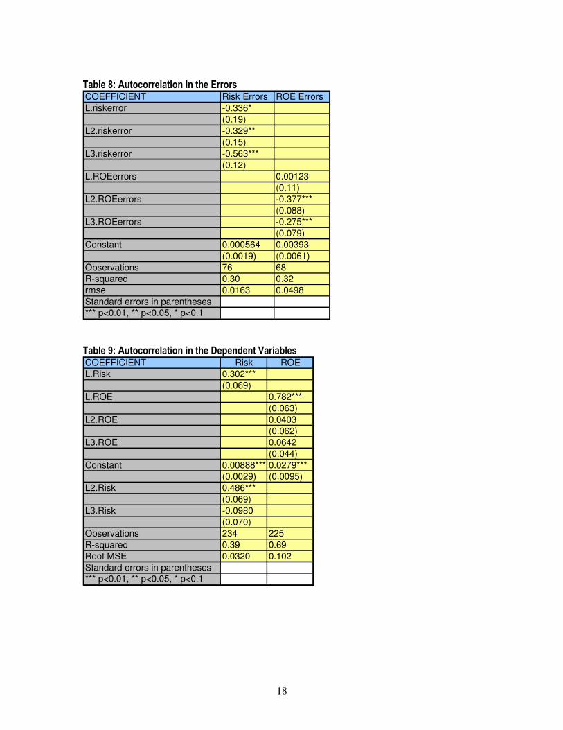
3. Autocorrelation:
For both the Repayment and Profitability Models, autocorrelation in the errors is a problem;
however, it is not highly significant. When regressing the errors on their own lags, we find that the first
lag in the Repayment Model is significant, but only at the 90% confidence level. The first lag in the ROE
model is not significant. However, in both models, the second and third lags are highly significant, at
the 95% and 99% levels (see Table 8).
When testing for autocorrelation in the dependent variables by regressing these variables on
their own lags, we find highly significant first lags in both models (See Table 9). This indicates a serious
autocorrelation problem. Fortunately, this will not bias my coefficients; however, it means that my
standard errors will be too small, causing my confidence intervals to be overestimated.
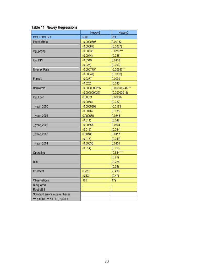
To attempt to fix the autocorrelation problems in the dependent variables and the errors, I ran
“newey” regressions on both models. In the repayment model, all of the independent variables remain
insignificant. In the profitability model, per-capita GDP becomes even more significant and unemp_Rate
and Borrowers both reach statistical significance at the 95% and 99% levels, respectively.
9
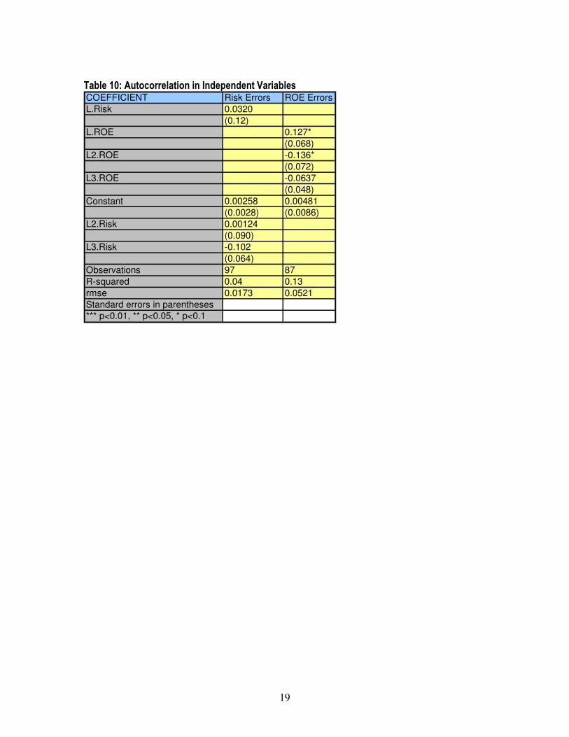
A test for autocorrelation in the independent variables shows no statistically significant lags at
the 95% level or higher (see Table 10). Therefore, there does not appear to be autocorrelation in the
independent variables.
4. Random Effects Assumption:
For the Random Effects model to be accurate, we must assume that the unobservable fixed
effects (αi) are orthogonal to the independent variables (Xit). This is a somewhat difficult assumption to
make. For example, an unobserved fixed effect in an MFI—like “management experience” or
“management performance”—could definitely be correlated with the explanatory variables. However,
the Hausman Test indicates that the coefficients in the Random Effects model are not significantly
different than in the Fixed Effects Model; therefore, the model should not be terribly biased.
5. Omitted Variable Bias:
Considering the various economic, social and cultural factors that can affect repayment rates
and MFI profitability, it is doubtful that my models incorporate all of the variables influencing the data.
However, in view of the large number of controls used, any remaining omitted variables are not likely to
significantly impact the results. Furthermore, use of the Random Effects model should capture many of
the unobservable characteristics of the microfinance organizations.
VI. Conclusion
In the Repayment Model, there are no statistically significant explanatory variables. This
appears to indicate that the macroeconomic environment has no impact on MFI repayment rates.
Strangely, the percentage of female borrowers also seems to have no impact on repayment. Although
10
further research with larger, randomly selected data-sets is required to corroborate these findings, there
does appear to be a strong indication that MFIs will achieve similar repayment rates no matter the
macro-economic environment in which they are located.
In the Profitability Model, things are not as straightforward. The initial model shows a strong
positive impact of per-capita GDP on ROE. However, this regression is misleading, as Graph 1
illustrates. It is more meaningful to separate the model into low- and high-income developing nation
models. In this case, we can clearly see that income has no impact on ROE in low-income developing
countries, although it does have a significant impact in high-income developing counties. Indeed,
among high-income developing nations, a $1000US increase in per-capita GDP causes more than a
7% increase in the ROE of microfinance organizations. Therefore, coupled with our earlier findings, we
would expect that MFIs would find the highest ROEs in Latin America, where the per-capita GDP is the
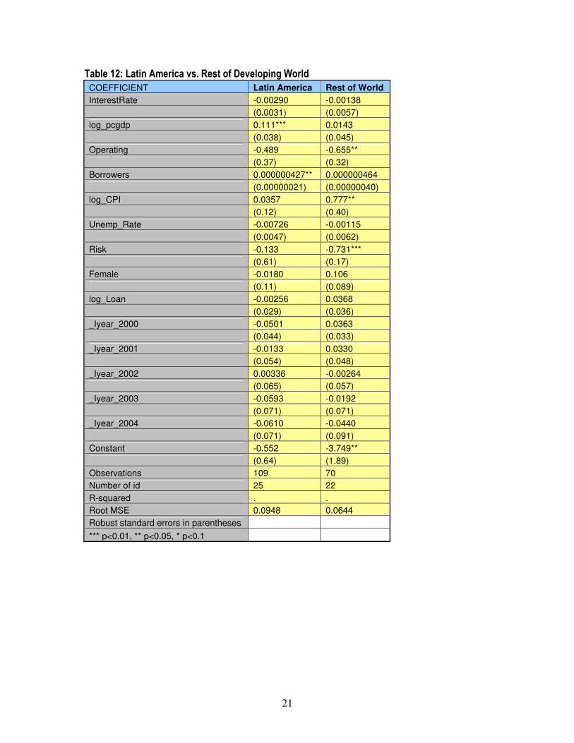
highest. And we do indeed find this to be the case. In fact, a glance at the Profitability Model using only
Latin America countries shows a highly significant positive relationship between income and ROE;
whereas, a regression with the rest of the developing world shows no significant relationship (see Table
12). However, before you run to Latin America to start an MFI, it should be borne in mind that this
region also has the most established and experienced MFIs in the world. Therefore, it could very well
be that my model is simply picking up the strength and depth of the microfinance sector in Latin
America. (Interestingly, the “Rest of the World” regression in Table 12 shows a statistically significant
relationship between inflation and ROE, and a highly significant negative relationship between Risk and
ROE. However, it should be borne in mind that this regression only includes 70 observations).
Another interesting yet inconclusive aspect of this study is the fall in ROE after big jumps in
per-capita GDP (see Graph 2). Although there are really too few years to properly analyze this type of
trend, the discontinuous impact is striking. The fall in ROE might be caused by the fact that, as income
rises, people become less dependent on microfinance institutions and begin to borrow less, thereby
11
causing the decrease in ROE. This has fascinating implications considering the fact that MFIs are
attempting to combat poverty by increasing income, all the while this increasing income could in fact be
contributing to their own falling profits. But, again, further research is needed with a larger and
randomly selected data-set.
Aside from this, however, one conclusive finding is that in both models (including the low- and
high-income ROE models) we find that inflation was not statistically significant. So, although Vanroose
found that there is greater microfinance outreach in countries with high inflation, this is probably
because international organizations are specifically targeting those countries; not because high inflation
rates themselves are having an impact on MFI performance.
12
Appendix I—Tables:
Table 2: Independent Variables Independent Variable (w/stata name in parentheses)
Description Justification for Inclusion / Exclusion
Consumer Price Index (log_CPI)
Log of consumer price index. Proxy for inflation.
Main causal variable: see above discussion.
Interest Rate (InterestRate)
Banks prime lending rates. Proxy for country-wide interest rates.
Main causal variable: see above discussion
Per Capita GDP (log_pcgdp)
Log of Per Capita GDP. Main causal variable: see above description
Unemployment Rate (Unemp_Rate)
Total unemployment rate. Main causal variable: see above description
Female (Female)
Percentage of female borrowers in MFI. Control for effects of gender on MFI success
Loan (Loan)
Log of Average Loan Size Control for effects of loan size on success of MFIs.
Operating Expenses (Operating)
Operating Expenses / Average Total Assets
Control for effects of operating expenses on MFI profitability. Note: Only used in ROE model.
Portfolio at Risk (Risk) Measure of borrower repayment: Portfolio at Risk > 30 days / Gross Loan Portfolio
Control for effects of delinquency on ROE. Note: Only used in ROE model.
Borrowers (Borrowers) Number of borrowers in MFI. Control for size of MFI in random effects model (cannot use pweights).
Established (Established) Year MFI was established Had little or no impact: Not used in models. Type of MFI (Type) Type of MFI (ie: bank, cooperative, non-
bank financial institution, NGO, rural bank or other)
Had little or no impact: Not used in models.
Region (Region) Region where the MFI is located (ie: Sub-Saharan Africa, East Asia & the Pacific, Eastern Europe and Central Asia, Latin America and the Caribbean, Middle East and North Africa and South Asia).
Used in high-income profitability model.
13
Table 3: Pooled OLS POLS POLS
COEFFICIENT ROE Risk
InterestRate -0.000499 0.000442
(0.0016) (0.00068)
pcgdp 0.0000703*** -0.00000128
(0.0000063) (0.0000015)
Operating -0.524***
(0.17)
CPI -0.00132*** -0.0000667
(0.00045) (0.00011)
Unemp_Rate -0.00634*** -0.000953**
(0.0019) (0.00039)
Female 0.00271 -0.0361*
(0.062) (0.019)
Loan 0.00000598 0.0000102
(0.000022) (0.0000074)
Risk -0.945***
(0.35)
_Iyear_2000 -0.00843 0.000708
(0.044) (0.0095)
_Iyear_2001 0.0418 0.00162
(0.043) (0.010)
_Iyear_2002 0.0551 -0.00643
(0.044) (0.0099)
_Iyear_2003 0.0393 -0.00387
(0.047) (0.012)
_Iyear_2004 0.0631 -0.00259
(0.049) (0.012)
Constant 0.367*** 0.0582*
(0.098) (0.029)
Observations 179 185
R-squared 0.74 0.34
Root MSE 0.0937 0.0220
Robust standard errors in parentheses
*** p<0.01, ** p<0.05, * p<0.1
14
Table 4: Between Regressions Between Between
COEFFICIENT Risk ROE
meanCPI 0.0000658 -0.00220**
(0.00015) (0.00092)
meanpcgdp -0.00000128* 0.0000637***
(0.00000066) (0.0000068)
meanIR 0.0000138 0.00175
(0.00038) (0.0011)
meanFemale -0.0610*** 0.165***
(0.015) (0.042)
meanUnemp -0.00129*** -0.00381***
(0.00034) (0.0012)
meanLoan 0.00000255 0.0000114
(0.0000050) (0.000014)
meanOperat -0.856***
(0.070)
meanRisk -0.577**
(0.29)
Constant 0.0730*** 0.355***
(0.028) (0.12)
Observations 295 330
R-squared 0.41 0.45
Root MSE 0.0182 0.106
Robust standard errors in parentheses
*** p<0.01, ** p<0.05, * p<0.1
15
Table 5: Random Effects Models
RE RE
COEFFICIENT Risk ROE
InterestRate -0.0000152 0.00196
(0.00078) (0.0022)
log_pcgdp -0.00323 0.0773**
(0.0055) (0.032)
log_CPI -0.0417 0.0911
(0.027) (0.098)
Unemp_Rate -0.000725 -0.00327
(0.00057) (0.0038)
Female -0.0369 0.0237
(0.028) (0.075)
Borrowers -0.0000000168 0.000000154
(0.000000035) (0.00000022)
log_Loan 0.00878 -0.00671
(0.0059) (0.020)
_Iyear_2000 -0.000849 -0.00680
(0.0068) (0.026)
_Iyear_2001 -0.0000960 0.0406
(0.010) (0.028)
_Iyear_2002 -0.00821 0.0602**
(0.011) (0.030)
_Iyear_2003 0.00366 0.0384
(0.017) (0.033)
_Iyear_2004 -0.00453 0.0385
(0.015) (0.035)
Operating -0.702***
(0.27)
Risk -0.472*
(0.26)
Constant 0.230* -0.702*
(0.14) (0.41)
Observations 185 179
Number of id 48 47
R-squared . .
Root MSE 0.0214 0.0789
Robust standard errors in parentheses
*** p<0.01, ** p<0.05, * p<0.1
16
Table 6: Interactions
Interaction Justification Significant?
Type*Unemp_Rate Is the impact of the unemployment rate significantly different depending on the type of MFI? (Types of MFIs include bank, cooperative, NGO, rural bank, non-bank financial institution and other)
No
Type*CPI Is the impact of inflation significantly different depending on the type of MFI? No Region*Unemp_Rate Is the impact of the unemployment rate significantly different depending on the region
where the MFI is located? (Regions include sub-Saharan Africa, East Asia & the Pacific, Latin America & the Caribbean, Middle East & North Africa, South-East Asia and Eastern Europe & Central Asia).
No
Region*CPI Is the impact of inflation significantly different depending on the region where the MFI is located?
No
Female*Region Is the impact of the percentage of female borrowers significantly different depending of where the MFI is located?
No
Female*Type Is the impact of the percentage of female borrowers significantly different depending on the type of MFI?
No
Risk*Female Is the impact of delinquency significantly different depending on the percentage of female borrowers?
No
Type*Operating Is the impact of operating expenses significantly different depending on the type of MFI? No Regulated*Operating Is the impact of operating expenses different depending on whether the MFI is regulated or
not? No
Region*pcgdp Is the impact of per capita gdp different depending on the region where the MFI is located? No Type*pcgdp Is the impact of per capita gdp different depending on the type of MFI? No Regulated*pcgdp Is the impact of per capita gdp different depending on whether the MFI is regulated? No
17
Table 7: Low-Income vs. High Income ROE Models Low-Income High-Income
COEFFICIENT ROE ROE
lowpcgdp -0.0000111
(0.000047)
InterestRate -0.00213 0.00802*
(0.0022) (0.0048)
log_CPI 0.0665 -0.129
(0.083) (0.11)
Unemp_Rate 0.00602 0.00274
(0.0058) (0.0057)
Borrowers 0.000000770* 0.000000176
(0.00000045) (0.00000021)
Risk -0.482** -1.133
(0.23) (0.81)
Female -0.158 -0.0674
(0.10) (0.11)
log_Loan -0.000634 0.0600
(0.027) (0.039)
_Iyear_2000 0.0143 -0.0189
(0.025) (0.069)
_Iyear_2001 0.0415 0.0987*
(0.027) (0.055)
_Iyear_2002 0.0561* 0.112
(0.033) (0.069)
_Iyear_2003 0.0298 0.0907
(0.034) (0.079)
_Iyear_2004 0.0104 0.0895
(0.044) (0.083)
highpcgdp 0.0000908***
(0.000020)
Region 0.140***
(0.035)
Constant -0.169 -0.510
(0.40) (0.71)
Observations 99 80
Number of id 33 18
R-squared . .
Root MSE 0.0668 0.0853
Robust standard errors in parentheses
*** p<0.01, ** p<0.05, * p<0.1
18
Table 8: Autocorrelation in the Errors COEFFICIENT Risk Errors ROE Errors
L.riskerror -0.336*
(0.19)
L2.riskerror -0.329**
(0.15)
L3.riskerror -0.563***
(0.12)
L.ROEerrors 0.00123
(0.11)
L2.ROEerrors -0.377***
(0.088)
L3.ROEerrors -0.275***
(0.079)
Constant 0.000564 0.00393
(0.0019) (0.0061)
Observations 76 68
R-squared 0.30 0.32
rmse 0.0163 0.0498
Standard errors in parentheses
*** p<0.01, ** p<0.05, * p<0.1
Table 9: Autocorrelation in the Dependent Variables COEFFICIENT Risk ROE
L.Risk 0.302***
(0.069)
L.ROE 0.782***
(0.063)
L2.ROE 0.0403
(0.062)
L3.ROE 0.0642
(0.044)
Constant 0.00888*** 0.0279***
(0.0029) (0.0095)
L2.Risk 0.486***
(0.069)
L3.Risk -0.0980
(0.070)
Observations 234 225
R-squared 0.39 0.69
Root MSE 0.0320 0.102
Standard errors in parentheses
*** p<0.01, ** p<0.05, * p<0.1
19
Table 10: Autocorrelation in Independent Variables COEFFICIENT Risk Errors ROE Errors
L.Risk 0.0320
(0.12)
L.ROE 0.127*
(0.068)
L2.ROE -0.136*
(0.072)
L3.ROE -0.0637
(0.048)
Constant 0.00258 0.00481
(0.0028) (0.0086)
L2.Risk 0.00124
(0.090)
L3.Risk -0.102
(0.064)
Observations 97 87
R-squared 0.04 0.13
rmse 0.0173 0.0521
Standard errors in parentheses
*** p<0.01, ** p<0.05, * p<0.1
20
Table 11: Newey Regressions
Newey2 Newey2
COEFFICIENT Risk ROE
InterestRate -0.0000307 0.00132
(0.00087) (0.0027)
log_pcgdp -0.00535 0.0786***
(0.0044) (0.028)
log_CPI -0.0349 0.0133
(0.025) (0.093)
Unemp_Rate -0.000775* -0.00687**
(0.00047) (0.0032)
Female -0.0277 0.0999
(0.023) (0.080)
Borrowers -0.0000000255 0.000000746***
(0.000000039) (0.00000014)
log_Loan 0.00671 0.00296
(0.0058) (0.022)
_Iyear_2000 -0.0000899 -0.0173
(0.0076) (0.035)
_Iyear_2001 0.000650 0.0345
(0.011) (0.042)
_Iyear_2002 -0.00857 0.0604
(0.012) (0.044)
_Iyear_2003 0.00180 0.0117
(0.017) (0.049)
_Iyear_2004 -0.00538 0.0151
(0.014) (0.053)
Operating -0.634***
(0.21)
Risk -0.226
(0.39)
Constant 0.220* -0.438
(0.13) (0.47)
Observations 185 179
R-squared . .
Root MSE . .
Standard errors in parentheses
*** p<0.01, ** p<0.05, * p<0.1
21
Table 12: Latin America vs. Rest of Developing World
COEFFICIENT Latin America Rest of World
InterestRate -0.00290 -0.00138
(0.0031) (0.0057)
log_pcgdp 0.111*** 0.0143
(0.038) (0.045)
Operating -0.489 -0.655**
(0.37) (0.32)
Borrowers 0.000000427** 0.000000464
(0.00000021) (0.00000040)
log_CPI 0.0357 0.777**
(0.12) (0.40)
Unemp_Rate -0.00726 -0.00115
(0.0047) (0.0062)
Risk -0.133 -0.731***
(0.61) (0.17)
Female -0.0180 0.106
(0.11) (0.089)
log_Loan -0.00256 0.0368
(0.029) (0.036)
_Iyear_2000 -0.0501 0.0363
(0.044) (0.033)
_Iyear_2001 -0.0133 0.0330
(0.054) (0.048)
_Iyear_2002 0.00336 -0.00264
(0.065) (0.057)
_Iyear_2003 -0.0593 -0.0192
(0.071) (0.071)
_Iyear_2004 -0.0610 -0.0440
(0.071) (0.091)
Constant -0.552 -3.749**
(0.64) (1.89)
Observations 109 70
Number of id 25 22
R-squared . .
Root MSE 0.0948 0.0644
Robust standard errors in parentheses
*** p<0.01, ** p<0.05, * p<0.1
22
Appendix II—Graphs:
Graph 1: Graph 2:
-.2
0.2
.4.6
RO
E
0 2000 4000 6000Per Capita GDP
Linear Fit Non-Parametric Relationship
Effect of Per Capita GDP on ROE: Lowess vs. OLS
-.
06
-.0
4-.
02
0.0
2R
esid
ual R
OE
-4 -2 0 2 4 6Years to Improvement
How ROE changes with Big Improvements in Per Capita GDP
Graph 3: Graph 4:
-1.5
-1-.
50
.51
RO
E
0 500 1000 1500Per Capita GDP
lowess ROE lowpcgdp (Net Op. Inc., less Taxes)/ Period Av. Equity
Effect of Per Capita GDP on Profitability in Low-Income Nations
-1.5
-1-.
50
.51
Retu
rn o
n E
qu
ity
2000 3000 4000 5000 6000 7000Per Capita GDP
lowess ROE highpcgdp (Net Op. Inc., less Taxes)/ Period Av. Equity
Effect of Per Capita GDP on Profitability in High-Income Nations
23
Graph 5: ROE Normality 0
.51
1.5
22
.5D
en
sity
-1.5 -1 -.5 0 .5 1(Net Op. Inc., less Taxes)/ Period Av. Equity
Graph 6: Affect of Region on ROE
-1-.
50
.5R
etu
rn o
n E
qu
ity
1 2 3 4 5Region
lowess ROE Region (Net Op. Inc., less Taxes)/ Period Av. Equity
ROE per Region in High-Income Developing Nations

24
Appendix III—.do file:
Start-up: #delimit; pause on; clear; set mem 15m; set more off; log using MFI1, replace; cd "C:\data\QM2"; use MFIFinal6.dta;
encode MFI, gen(id); tsset id year, yearly; xi i.year;
Trying different controls: /*POLS */ reg Risk InterestRate pcgdp CPI Unemp_Rate Loan _Iyear*; reg Risk InterestRate pcgdp CPI Unemp_Rate Female Loan _Iyear*; hettest; reg Risk InterestRate pcgdp CPI Unemp_Rate Female Loan _Iyear* [pweight=Borrowers]; reg Risk InterestRate pcgdp Operating CPI Unemp_Rate Female Loan _Iyear* [pweight=Borrowers]; reg ROA InterestRate pcgdp CPI Unemp_Rate Risk Loan _Iyear*; reg ROA InterestRate pcgdp CPI Unemp_Rate Female Loan _Iyear*; hettest; reg ROE InterestRate pcgdp CPI Unemp_Rate Risk Loan _Iyear*; reg ROE InterestRate pcgdp CPI Unemp_Rate Female Loan _Iyear*; hettest; reg ROE InterestRate pcgdp CPI Unemp_Rate Female Loan _Iyear* [pweight=Borrowers]; reg ROE InterestRate pcgdp Operating CPI Unemp_Rate Female Risk Loan _Iyear* [pweight=Borrowers];
POLS: reg Risk InterestRate pcgdp Operating CPI Unemp_Rate Female Loan _Iyear* [pweight=Borrowers]; reg ROE InterestRate pcgdp Operating CPI Unemp_Rate Female Risk Loan _Iyear* [pweight=Borrowers];
FE vs. RE: /*Risk - FE vs. RE*/ xtreg Risk InterestRate pcgdp CPI Unemp_Rate Female Loan Borrowers _Iyear*, robust i(id) fe; est store fe; xtreg Risk InterestRate pcgdp CPI Unemp_Rate Female Loan Borrowers _Iyear*, robust i(id); hausman fe; gen log_CPI=ln(CPI);

25
gen log_Loan=ln(Loan); gen log_pcgdp=ln(pcgdp); /*Need to try with logs:*/ xtreg Risk InterestRate log_pcgdp log_CPI Unemp_Rate Female log_Loan Borrowers _Iyear*, robust i(id) fe; est store fe; xtreg Risk InterestRate log_pcgdp log_CPI Unemp_Rate Female log_Loan Borrowers _Iyear*, robust i(id); hausman fe; /*We accept the null hypothesis of no difference between the coefficients, so we should use the RE estimator since it is both efficient and unbiased.*/ /*ROE - FE vs. RE*/ xtreg ROE InterestRate log_pcgdp Operating log_CPI Unemp_Rate Risk Female Borrowers log_Loan _Iyear*, robust i(id) fe; est store fe; xtreg ROE InterestRate log_pcgdp Operating log_CPI Unemp_Rate Risk Female Borrowers log_Loan _Iyear*, robust i(id); hausman fe; /*Want to use RE model*/
Non-Parametric Tests: /*Risk Non-parametric tests*/ gen unempType_inter= Type* Unemp_Rate; xtreg Risk InterestRate log_pcgdp log_CPI Unemp_Rate Type unemp Type_inter Female log_Loan _Iyear*, robust i(id); gen TypeCPI_inter=Type* log_CPI; xtreg Risk InterestRate log_pcgdp log_CPI Unemp_Rate Female Type TypeCPI_inter log_Loan _Iyear*, robust i(id); gen RegionUn_inter=Region* Unemp_Rate; xtreg Risk InterestRate log_pcgdp log_CPI Unemp_Rate Female Region RegionUn_inter log_Loan _Iyear*, robust i(id); gen RegionCPI_inter=Region* log_CPI; xtreg Risk InterestRate log_pcgdp log_CPI Unemp_Rate Female Region RegionCPI_inter log_Loan _Iyear*, robust i(id); gen Female_Region=Female*Region; xtreg Risk InterestRate log_pcgdp log_CPI Unemp_Rate Female Region Female_Region log_Loan _Iyear*, robust i(id); gen FemaleType_inter=Female*Type; xtreg Risk InterestRate log_pcgdp log_CPI Unemp_Rate Female Type FemaleType_inter log_Loan _Iyear*, robust i(id); /*ROE Non-parametric tests*/ xtreg ROE InterestRate log_pcgdp log_CPI Unemp_Rate Risk Type unempType_inter Female log_Loan _Iyear*, robust i(id);

26
xtreg ROE InterestRate log_pcgdp log_CPI Unemp_Rate Risk Female Type TypeCPI_inter log_Loan _Iyear*, robust i(id); xtreg ROE InterestRate log_pcgdp log_CPI Unemp_Rate Risk Female Region RegionUn_inter log_Loan _Iyear*, robust i(id); xtreg ROE InterestRate log_pcgdp log_CPI Unemp_Rate Risk Female Region RegionCPI_inter log_Loan _Iyear*, robust i(id); xtreg ROE InterestRate log_pcgdp log_CPI Unemp_Rate Risk Female Region Female_Region log_Loan _Iyear*, robust i(id); xtreg ROE InterestRate log_pcgdp log_CPI Unemp_Rate Risk Female Type FemaleType_inter log_Loan _Iyear*, robust i(id); gen RiskFem_inter=Risk*Female; xtreg ROE InterestRate log_pcgdp log_CPI Unemp_Rate Risk RiskFem_inter Female Loan _Iyear*, robust i(id); /*Operating Expenses*/ xtreg ROE InterestRate log_pcgdp log_CPI Operating Unemp_Rate Risk Female Loan _Iyear*, robust i(id); pwcorr Operating Female ROE Risk; gen oper_type= Type* Operating; xtreg ROE InterestRate log_pcgdp log_CPI Operating oper_type Type Unemp_Rate Risk Female Loan _Iyear*, robust i(id); gen Reg_oper=Regulated*Operating; xtreg ROE InterestRate log_pcgdp log_CPI Operating Reg_oper Regulated Unemp_Rate Risk Female Loan _Iyear*, robust i(id); */More interactions:*/ gen gdpReg_inter=pcgdp*Region; gen gdpType_inter=pcgdp*Type; gen gdpRegu_inter=pcgdp*Regulated; xtreg ROE InterestRate pcgdp Region gdpReg_inter Operating log_CPI Unemp_Rate Risk Female log_Loan _Iyear*, robust i(id); xtreg ROE InterestRate pcgdp Type gdpType_inter Operating log_CPI Unemp_Rate Risk Female log_Loan _Iyear*, robust i(id); xtreg ROE InterestRate pcgdp Regulated gdpRegu_inter Operating log_CPI Unemp_Rate Risk Female log_Loan _Iyear*, robust i(id); /*Although it appeared that more women lead to fewer profits, this was only because of the OMV of operating expenses. Apparently, Female was picking up the effects of Operating Expenses, since banks with a higher percentage of women tend to have higher operating expenses.*/
Final Models: /*Risk Model:*/ xtreg Risk InterestRate log_pcgdp log_CPI Unemp_Rate Female Borrowers log_Loan _Iyear*, robust i(id); /*Profitability Model:*/
27
xtreg ROE InterestRate log_pcgdp Operating Borrowers log_CPI Unemp_Rate Risk Female log_Loan _Iyear*, robust i(id); twoway (lfitci log_pcgdp ROE) (scatter log_pcgdp ROE), title(Effect of Per Capita GDP on Profitability) xtitle(Return on Equity) ytitle(Log of Per Capita GDP);
Between Estimator: /*Between Estimator*/ egen meanRisk=mean(Risk), by(id); egen meanCPI=mean(CPI), by(id); egen meanpcgdp=mean(pcgdp), by(id); egen meanIR=mean(InterestRate), by(id); egen meanFemale=mean(Female), by(id); egen meanUnemp=mean( Unemp_Rate), by(id); egen meanOperat=mean( Operating), by(id); egen meanLoan=mean(Loan), by(id); reg meanRisk meanCPI meanpcgdp meanIR meanFemale meanUnemp meanLoan; /*For the Risk model, it appears in the cross-section, MFIs with high risk have more men and less unemployment.*/ egen meanROE=mean(ROE), by(id); reg meanROE meanLoan meanOperat meanUnemp meanFemale meanIR meanpcgdp meanCPI meanRisk; /*In the cross-section, MFIs with higher ROE tend to high per capita GDP and low operating expenses.*/
Exploring Effect of Per Capita GDP on ROE: /*Exploring Effect of Per Capita GDP on ROE*/ gen bigimp=0 if var62==1; for num 1/3: replace bigimp=X if var62[_n-X]==1; for num 1/3: replace bigimp=-X if var62[_n+X]==1; xi i.year i.id; reg ROE _Iid* _Iyear*; predict uhat, resid; lowess uhat bigimp, gen(incsm); sort bigimp; label var bigimp "Years to Improvement"; label var incsm "Residual ROE"; line incsm bigimp, title("How ROE changes with Big Improvements in Per Capita GDP") xline(0); twoway (lfit ROE log_pcgdp) (lowess ROE log_pcgdp), legend(label (1 Linear Fit) label(2 Non-Parametric Relationship)) ytitle("ROE") title("Effect of Per Capita GDP on ROE: Lowess vs. OLS"); gen lowincome=log_pcgdp if log_pcgdp<=5.5; gen medincome=log_pcgdp if log_pcgdp>5.5 & log_pcgdp<8; gen highincome=log_pcgdp if log_pcgdp>=8;
28
xtreg ROE InterestRate medincome Operating log_CPI Unemp_Rate Risk Female log_Loan _Iyear*, robust i(id); twoway (lfit ROE pcgdp) (lowess ROE pcgdp), legend(label (1 Linear Fit) label(2 Non-Parametric Relationship)) ytitle("ROE") title("Effect of Per Capita GDP on ROE: Lowess vs. OLS"); xtreg ROE InterestRate lowpcgdp Operating log_CPI Unemp_Rate Risk Female log_Loan _Iyear*, robust i(id); twoway (lfit ROE lowpcgdp) (lowess ROE lowpcgdp), legend(label (1 Linear Fit) label(2 Non-Parametric Relationship)) ytitle("ROE") title("Effect of Per Capita GDP on ROE: Lowess vs. OLS"); twoway (lowess ROE pcgdp) (scatter ROE pcgdp), title(Effect of Per Capita GDP on Profitability) xtitle(Per Capita GDP) ytitle(ROE); gen lowpcgdp=pcgdp if pcgdp< 1500; gen highpcgdp=pcgdp if pcgdp>=1500;
Low- vs. High-Income Models: /*Low levels of Per Capita GDP:*/ xtreg ROE InterestRate lowpcgdp Operating log_CPI Unemp_Rate Risk Female log_Loan _Iyear*, robust i(id); twoway (lowess ROE lowpcgdp) (scatter ROE lowpcgdp), title(Effect of Per Capita GDP on Profitability in Low-Income Nations) xtitle(Return on Equity) ytitle(Per Capita GDP); xtreg Risk InterestRate lowpcgdp log_CPI Unemp_Rate Female log_Loan _Iyear*, robust i(id); /*Low levels interactions:*/ xtreg ROE InterestRate lowpcgdp log_CPI Unemp_Rate Risk Type unempType_inter Female log_Loan _Iyear*, robust i(id); xtreg ROE InterestRate lowpcgdp log_CPI Unemp_Rate Risk Female Type TypeCPI_inter log_Loan _Iyear*, robust i(id); xtreg ROE InterestRate lowpcgdp log_CPI Unemp_Rate Risk Female Region RegionUn_inter log_Loan _Iyear*, robust i(id); xtreg ROE InterestRate lowpcgdp log_CPI Unemp_Rate Risk Female Region RegionCPI_inter log_Loan _Iyear*, robust i(id); xtreg ROE InterestRate lowpcgdp log_CPI Unemp_Rate Risk Female Region Female_Region log_Loan _Iyear*, robust i(id); xtreg ROE InterestRate lowpcgdp log_CPI Unemp_Rate Risk Female Type FemaleType_inter log_Loan _Iyear*, robust i(id); gen RiskFem_inter=Risk*Female; xtreg ROE InterestRate lowpcgdp log_CPI Unemp_Rate Risk RiskFem_inter Female Loan _Iyear*, robust i(id); /*High levels of Per Capita GDP:*/

29
xtreg ROE highpcgdp Region Operating log_CPI Unemp_Rate Risk log_Loan _Iyear*, robust i(id); twoway (lowess ROE highpcgdp) (scatter ROE highpcgdp), title(Effect of Per Capita GDP on Profitability in High-Income Nations) xtitle(Return on Equity) ytitle(Per Capita GDP); xtreg Risk InterestRate highpcgdp log_CPI Unemp_Rate Female log_Loan _Iyear*, robust i(id); xtreg ROE InterestRate highpcgdp log_CPI Unemp_Rate Risk Type unempType_inter Female log_Loan _Iyear*, robust i(id); xtreg ROE InterestRate highpcgdp log_CPI Unemp_Rate Risk Female Type TypeCPI_inter log_Loan _Iyear*, robust i(id); xtreg ROE InterestRate highpcgdp log_CPI Unemp_Rate Risk Female Region RegionUn_inter log_Loan _Iyear*, robust i(id); xtreg ROE InterestRate highpcgdp log_CPI Unemp_Rate Risk Female Region RegionCPI_inter log_Loan _Iyear*, robust i(id); xtreg ROE InterestRate highpcgdp log_CPI Unemp_Rate Risk Female Region Female_Region log_Loan _Iyear*, robust i(id); xtreg ROE InterestRate highpcgdp log_CPI Unemp_Rate Risk Female Type FemaleType_inter log_Loan _Iyear*, robust i(id); gen RiskFem_inter=Risk*Female; xtreg ROE InterestRate highpcgdp log_CPI Unemp_Rate Risk RiskFem_inter Female Loan _Iyear*, robust i(id); /*Region statistically significant in higher income nations:*/ xtreg ROE InterestRate highpcgdp log_CPI Unemp_Rate Risk Region Female Loan _Iyear*, robust i(id); twoway (lowess ROE Region) (scatter ROE Region) if pcgdp>=1500, title(ROE per Region in High-Income Developing Nations) xtitle(Region) ytitle(Return on Equity);
Quadratic Time Check: /*Checking for quadratic time trend.*/ gen tsq=year^2; xi i.id; reg Risk InterestRate log_pcgdp log_CPI Unemp_Rate Female log_Loan year tsq _Iid*, robust; reg ROE InterestRate log_pcgdp Operating log_CPI Unemp_Rate Risk Female log_Loan year tsq _Iid*, robust;
Autocorrelation: /*Autocorrelation in Risk errors:*/ xtreg Risk InterestRate log_pcgdp log_CPI Unemp_Rate Female log_Loan _Iyear*, robust i(id); predict riskerror, e; reg riskerror L.riskerror L2.riskerror L3.riskerror; /*Lags 2 & 3 significant.*/

30
/*Autocorrelation in ROE errors*/ xtreg ROE InterestRate log_pcgdp Operating log_CPI Unemp_Rate Risk Female log_Loan _Iyear*, robust i(id); predict ROEerrors, e; reg ROEerror L.ROEerror L2.ROEerror L3.ROEerror; /*Lags 2 & 3 significant*/ /*Autocorrelation in Dependent variables:*/ reg Risk L.Risk L2.Risk L3.Risk; /*1st two lags significant.*/ reg ROE L.ROE L2.ROE L3.ROE; /*Only 1st lag significant (but highly significant).*/ /*Autocorrelation in independent variables.*/ xtreg Risk InterestRate log_pcgdp log_CPI Unemp_Rate Female log_Loan _Iyear*, robust i(id); regress riskerror L.Risk L2.Risk L3.Risk; /*Nothing significant*/ reg ROEerrors L.ROE L2.ROE L3.ROE; /*Nothing significant.*/
Newey Regressions: xi3: newey2 Risk InterestRate log_pcgdp log_CPI Unemp_Rate Female Borrowers log_Loan i.year, force lag(2); xi3: newey2 ROE InterestRate log_pcgdp Operating Borrowers log_CPI Unemp_Rate Risk Female log_Loan i.year, force lag(2); xi3: newey2 ROE InterestRate log_pcgdp Operating Borrowers log_CPI Unemp_Rate Risk Female log_Loan i.year, force lag(3);
Substantive Effects: estsimp reg ROE InterestRate highpcgdp Operating Borrowers log_CPI Unemp_Rate Risk Female log_Loan _Iyear*; setx mean; setx highpcgdp max; simqi; setx mean; simqi; sum ROE; setx mean; simqi; sum highpcgdp; setx highpcgdp 3295.426; simqi;
31
Latin America vs. Rest of Developing World:
xtreg ROE InterestRate log_pcgdp Operating Borrowers log_CPI Unemp_Rate Risk Female log_Loan _Iyear* if Region==4, robust i(id);

32
Appendix IV—Bibliography:
-- Armendáriz de Aghion, Beatriz & Morduch, Jonathan. The Economics of Microfinance. (2005): Massachusetts Institute of Technology. Cambridge, Massachusetts. -- Crabb, Peter. “Foreign Exchange Risk Management Practices of Microfinance Institutions.” Journal of Microfinance. (Winter, 2004). Retrieved from: http://marriottschool.byu.edu/esrreview/articles/article108.pdf -- Goldfajn, Ilan & Rigobon, Roberto. “Hard Currency and Financial Development.” Department of Economics, PUC-Rio (Brazil). (Dec. 2000). Retrieved from: http://econpapers.repec.org/paper/riotexdis/438.htm -- Japonica Intersect. “Microfinance for Profit.” (Feb. 2005). Retrieved from: www.japonicaintersectoral.com/PDF%20Files/MF.pdf -- Ledgerwood, Joanna. Microfinance Handbook: An Institutional and Financial Perspective. (1999): The World Bank. Washington D.C. -- Mcguire, Paul & Conroy, John D. “Effects on Microfinance of the 1997-1998 Asian Financial Crisis.” Banking with the Poor Newsletter. (June 1998), No 11. Retrieved from: http://www.bwtp.org/publications/pub/effects_on_microfinance.pdf -- Vander Weele, Ken & Markovich, Patricia. “Managing High and Hyper-Inflation in Microfinance: Opportunity International’s Experiences in Bulgaria and Russia.” (Aug. 2001). Retrieved from: http://www.microlinks.org/ev_en.php?ID=7412_201&ID2=DO_TOPIC -- Vanroose, Annabel. “The uneven development of microfinance: A Latin-American perspective.” Working Papers CEB from Université Libre de Bruxelles, Solvay Business School, Centre Emile Bernheim (CEB). (Oct. 2006). Retrieved from: http://econpapers.repec.org/paper/solwpaper/06-021.htm -- Walter, Ingo and Krauss, Nicolas A., "Can Microfinance Reduce Portfolio Volatility?" (November 9, 2006). Retrieved from: http://ssrn.com/abstract=943786 -- Yunus, Muhammad. Banker to the Poor. (2003): PublicAffairs. New York, NY.