The ICDAR/GREC 2013 Music Scores Competitionon Staff Removal

V.C Kieu∗†, Alicia Fornes ‡, Muriel Visani†, Nicholas Journet∗, and Anjan Dutta‡∗Laboratoire Bordelais de Recherche en Informatique - LaBRI, University of Bordeaux I, Bordeaux, France†Laboratoire Informatique, Image et Interaction - L3i, University of La Rochelle, La Rochelle, France

‡Computer Vision Center - Dept. of Computer Science. Universitat Autonoma de Barcelona, Ed.O, 08193, Bellaterra, SpainEmail: {vkieu, journet}@labri.fr, {afornes, adutta}@cvc.uab.es, muriel.visani@univ-lr.fr

Abstract—The first competition on music scores that wasorganized at ICDAR and GREC in 2011 awoke the interest ofresearchers, who participated both at staff removal and writeridentification tasks. In this second edition, we propose a staffremoval competition where we simulate old music scores. Thus,we have created a new set of images, which contain noise and 3Ddistortions. This paper describes the distortion methods, metrics,the participant’s methods and the obtained results.

Keywords—Competition, Music scores, Staff Removal.

I. INTRODUCTION

Optical Music Recognition (OMR) has been an activeresearch field for years. Many staff removal algorithms havebeen proposed [1], [2] as a first step in the OMR systems.However, there is still room for research, especially in the caseof degraded music scores. At ICDAR [3] and GREC 2011, weorganized the first edition of the music scores competition.For the staff removal task, we created several sets of distortedimages (each set corresponding to a different kind of distor-tion) and compared the robustness of the participants’ methods.After GREC 2011, we extended the staff removal competition[4] by generating a new set of images combining differentdistortions at different levels. The results demonstrated thatmost methods significantly decrease the performance whencoping with a combination of distortions.

In this second edition of the competition, we have gener-ated new images that emulate typical degradations appearing inold handwritten documents. Two types of degradations (localnoise and 3D distortions) have been applied on the 1000images from the original CVC-MUSCIMA database [5].

The rest of the paper is organized as follows. Firstly, wedescribe the degradation models and the dataset used for thecompetition. Secondly, we present the participants’ methods,the evaluation metrics, and we analyze the results.

II. ICDAR/GREC 2013 DATABASE

For comparing the robustness of the different participants’staff removal algorithms, we have applied the 3D distortionand the local noise degradation models described hereafter tothe original CVC-MUSCIMA database [5], which consists of1000 music sheets written by 50 different musicians.

A. Degradation Models

1) 3D Degradation Model: This degradation model aimsat mimicking some challenging distortions for staff removal

algorithms, such as skews, curvatures and rotations. Differingfrom the 2D model used for GREC 2011, our new 3D model[6] generates much more realistic images containing dents,small folds, torns. . . This 3D degradation model can distort thestaff lines, making their detection and removal more difficult. Itis based on 3D meshes and texture coordinate generation. Themain idea is that we get multiple 3D meshes of old documentpages using real ancient documents and a 3D scanner. Then,we wrap any 2D image on these meshes using some wrappingfunctions which are specifically adapted to document images.

2) Local Noise Model: Some old documents’ defects suchas ink splotches and white specks or streaks might lead forinstance to disconnections of the staff lines or to the additionof dark specks connected to a staff line which can be confusedwith musical symbols. In order to simulate such degradations,which are very challenging for staff removal algorithms, weapply our local noise model described in [7]. It consists inthree main steps. Firstly, the ”seed-points” (i.e. the centres oflocal noise regions) are selected so that they are more likely toappear near the foreground pixels (obtained by binarizing theinput grayscale image). Then, we add arbitrary shaped grey-level specks (in our case, the shape is an ellipse). The grey-level values of the pixels inside the noise regions are modifiedso as to obtain realistic looking bright and dark specks.

B. ICDAR/GREC 2013 Degraded Database

For the ICDAR/GREC 2013 staff removal competition,we generate a semi-synthetic database by applying the twodegradation models presented above to the 1000 images fromthe original CVC-MUSCIMA database. The obtained degradeddatabase consists in 6000 images: 4000 images for training and2000 images for testing the staff removal algorithms.

1) Training Set: The training set consists in 4000 semi-synthetic images generated from 667 out of the 1000 originalimages in the CVC-MUSCIMA database. This training set issplit into three subsets corresponding to different degradationtypes and levels of degradation, as described hereafter:

TrainingSubset1 contains 1000 images generated using the3D distortion model (c.f. sub-section II-A1) and two differentmeshes. The first mesh contains essentially a perspectivedistortion due to the scanning of a thick and bound page, whilethe second mesh has many small curves, folds and concaves.Both meshes are applied to the 667 original images. Then,1000 images (500 images per mesh) are randomly selectedfrom those 2× 667 = 1334 degraded images.

TrainingSubset2 contains 1000 images generated with threedifferent levels (i.e low, medium, and high levels) of localnoise. The different levels of noise are obtained by varyingthe number of seed-points and the average size of the noiseregions (see sub-section II-A2).

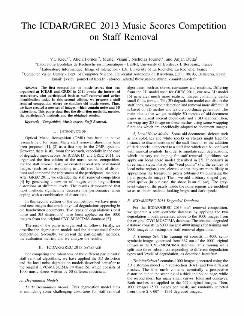
TrainingSubset3 (see Fig. 1) contains 2000 images gener-ated using both the 3D distortion and the local noise model.We obtain six different levels of degradation (the two meshesused for TrainingSubset1 × the three levels of distortion usedfor TrainingSubset2).

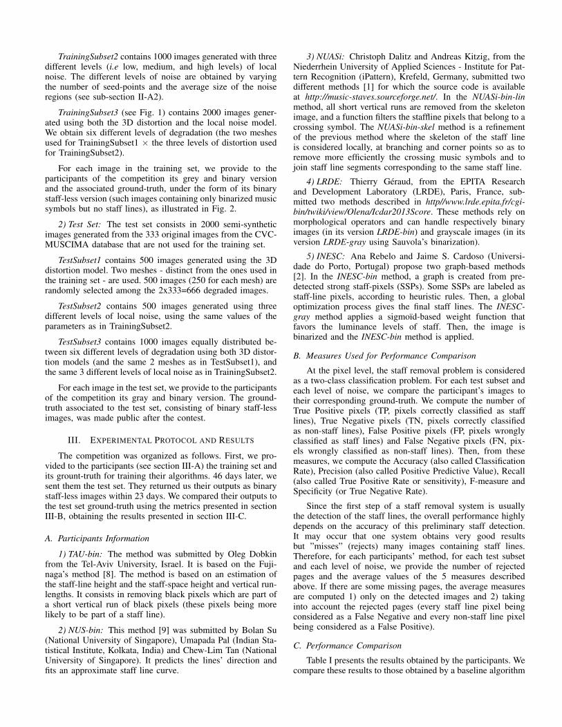
For each image in the training set, we provide to theparticipants of the competition its grey and binary versionand the associated ground-truth, under the form of its binarystaff-less version (such images containing only binarized musicsymbols but no staff lines), as illustrated in Fig. 2.

2) Test Set: The test set consists in 2000 semi-syntheticimages generated from the 333 original images from the CVC-MUSCIMA database that are not used for the training set.

TestSubset1 contains 500 images generated using the 3Ddistortion model. Two meshes - distinct from the ones used inthe training set - are used. 500 images (250 for each mesh) arerandomly selected among the 2x333=666 degraded images.

TestSubset2 contains 500 images generated using threedifferent levels of local noise, using the same values of theparameters as in TrainingSubset2.

TestSubset3 contains 1000 images equally distributed be-tween six different levels of degradation using both 3D distor-tion models (and the same 2 meshes as in TestSubset1), andthe same 3 different levels of local noise as in TrainingSubset2.

For each image in the test set, we provide to the participantsof the competition its gray and binary version. The ground-truth associated to the test set, consisting of binary staff-lessimages, was made public after the contest.

III. EXPERIMENTAL PROTOCOL AND RESULTS

The competition was organized as follows. First, we pro-vided to the participants (see section III-A) the training set andits grount-truth for training their algorithms. 46 days later, wesent them the test set. They returned us their outputs as binarystaff-less images within 23 days. We compared their outputs tothe test set ground-truth using the metrics presented in sectionIII-B, obtaining the results presented in section III-C.

A. Participants Information

1) TAU-bin: The method was submitted by Oleg Dobkinfrom the Tel-Aviv University, Israel. It is based on the Fuji-naga’s method [8]. The method is based on an estimation ofthe staff-line height and the staff-space height and vertical run-lengths. It consists in removing black pixels which are part ofa short vertical run of black pixels (these pixels being morelikely to be part of a staff line).

2) NUS-bin: This method [9] was submitted by Bolan Su(National University of Singapore), Umapada Pal (Indian Sta-tistical Institute, Kolkata, India) and Chew-Lim Tan (NationalUniversity of Singapore). It predicts the lines’ direction andfits an approximate staff line curve.

3) NUASi: Christoph Dalitz and Andreas Kitzig, from theNiederrhein University of Applied Sciences - Institute for Pat-tern Recognition (iPattern), Krefeld, Germany, submitted twodifferent methods [1] for which the source code is availableat http://music-staves.sourceforge.net/. In the NUASi-bin-linmethod, all short vertical runs are removed from the skeletonimage, and a function filters the staffline pixels that belong to acrossing symbol. The NUASi-bin-skel method is a refinementof the previous method where the skeleton of the staff lineis considered locally, at branching and corner points so as toremove more efficiently the crossing music symbols and tojoin staff line segments corresponding to the same staff line.

4) LRDE: Thierry Geraud, from the EPITA Researchand Development Laboratory (LRDE), Paris, France, sub-mitted two methods described in http//www.lrde.epita.fr/cgi-bin/twiki/view/Olena/Icdar2013Score. These methods rely onmorphological operators and can handle respectively binaryimages (in its version LRDE-bin) and grayscale images (in itsversion LRDE-gray using Sauvola’s binarization).

5) INESC: Ana Rebelo and Jaime S. Cardoso (Universi-dade do Porto, Portugal) propose two graph-based methods[2]. In the INESC-bin method, a graph is created from pre-detected strong staff-pixels (SSPs). Some SSPs are labeled asstaff-line pixels, according to heuristic rules. Then, a globaloptimization process gives the final staff lines. The INESC-gray method applies a sigmoıd-based weight function thatfavors the luminance levels of staff. Then, the image isbinarized and the INESC-bin method is applied.

B. Measures Used for Performance Comparison

At the pixel level, the staff removal problem is consideredas a two-class classification problem. For each test subset andeach level of noise, we compare the participant’s images totheir corresponding ground-truth. We compute the number ofTrue Positive pixels (TP, pixels correctly classified as stafflines), True Negative pixels (TN, pixels correctly classifiedas non-staff lines), False Positive pixels (FP, pixels wronglyclassified as staff lines) and False Negative pixels (FN, pix-els wrongly classified as non-staff lines). Then, from thesemeasures, we compute the Accuracy (also called ClassificationRate), Precision (also called Positive Predictive Value), Recall(also called True Positive Rate or sensitivity), F-measure andSpecificity (or True Negative Rate).

Since the first step of a staff removal system is usuallythe detection of the staff lines, the overall performance highlydepends on the accuracy of this preliminary staff detection.It may occur that one system obtains very good resultsbut ”misses” (rejects) many images containing staff lines.Therefore, for each participants’ method, for each test subsetand each level of noise, we provide the number of rejectedpages and the average values of the 5 measures describedabove. If there are some missing pages, the average measuresare computed 1) only on the detected images and 2) takinginto account the rejected pages (every staff line pixel beingconsidered as a False Negative and every non-staff line pixelbeing considered as a False Positive).

C. Performance Comparison

Table I presents the results obtained by the participants. Wecompare these results to those obtained by a baseline algorithm

Fig. 1. From left to right: original image from the CVC-MUSCIMA database, and two images from TrainingSubset3 of the ICDAR/GREC 2013 databasegenerated using a high level of local noise and (respectively) mesh#1 and mesh#2.

Fig. 2. From left to right: an image from TrainingSubset3, its binary version and its binary staff-less version (ground-truth)

proposed by Dutta et al. [10] and based on the analysis ofneighboring components. For each line, the best method isin bold. Since the Precision is higher in some methods butwith a lower Recall, we select the winners according to theAccuracy and F-measure metrics. INESC-bin is the winner onthe TestSubset2 containing local noise, while LRDE-bin is thewinner on the TestSubsets 1 and 3, containing respectively3D distortions and a combination of 3D distortions and localnoise. It must also be noticed that most methods (includingthe baseline method) obtain quite similar performances.

We can also analyze the scores according to the kind andlevel of degradations. Concerning the 3D distortion (TestSub-set1), most methods seem less robust to perspective deforma-tion defects (Mesh 1) than to the presence of small curvesand folds (Mesh 2). In addition, the precision scores of everyparticipants decrease (on average of 13%) when the local noisein TestSubset2 is getting higher. Therefore, all the participants’methods are sensitive to the local noise degradation. Thetests carried out with images from TestSubset3, generated bycombining local noise and 3D distortions confirm that theresults decrease when the level of degradation is important.

IV. CONCLUSION

The second music scores competition on staff removalheld in ICDAR and GREC 2013 has raised a great interestfrom the research community, with 8 participant methods.The submitted methods have obtained very satisfying per-formance, although most methods significantly decrease theirperformance when dealing with a higher level of degradation.The presence of both sources of degradation (3D distortion +local noise) is especially challenging. We hope that our semi-synthetic database will become a benchmark for the researchon handwritten music scores in the near future.

ACKNOWLEDGEMENTS

This research was partially funded by the French NationalResearch Agency (ANR) via the DIGIDOC project, and the

spanish projects TIN2009-14633-C03-03 and TIN2012-37475-C02-02. We would also like to thank Anjan Dutta for providingthe baseline results.

REFERENCES

[1] C. Dalitz, M. Droettboom, B. Pranzas, and I. Fujinaga, “A ComparativeStudy of Staff Removal Algorithms,” Pattern Analysis and MachineIntelligence, IEEE Transactions on, vol. 30, no. 5, pp. 753–766, 2008.

[2] J. dos Santos Cardoso, A. Capela, A. Rebelo, C. Guedes, and J. Pinto daCosta, “Staff Detection with Stable Paths,” Pattern Analysis and Ma-chine Intelligence, IEEE Transactions on, vol. 31, no. 6, pp. 1134–1139,2009.

[3] A. Fornes, A. Dutta, A. Gordo, and J. Llados, “The ICDAR 2011Music Scores Competition: Staff Removal and Writer Identification,”in Document Analysis and Recognition (ICDAR), 2011 InternationalConference on. Beijing, China: IEEE, Sep. 2011, pp. 1511–1515.

[4] ——, “The 2012 Music Scores Competitions: Staff Removal and WriterIdentification,” in Graphics Recognition. New Trends and Challenges.Lecture Notes in Computer Science, Y.-B. Kwon and J.-M. Ogier, Eds.Springer, 2013, vol. 7423, pp. 173–186.

[5] ——, “CVC-MUSCIMA: A Ground Truth of Handwritten Music ScoreImages for Writer Identification and Staff Removal,” InternationalJournal on Document Analysis and Recognition (IJDAR), vol. 15, no. 3,pp. 243–251, 2012.

[6] V. Kieu, N. Journet, M. Visani, R. Mullot, and J. Domenger, “Semi-synthetic Document Image Generation Using Texture Mapping onScanned 3D Document Shapes,” in Accepted for publication in Docu-ment Analysis and Recognition (ICDAR), 2013 International Conferenceon, Washington, DC, USA, 2013.

[7] V. Kieu, M. Visani, N. Journet, J. P. Domenger, and R. Mullot,“A Character Degradation Model for Grayscale Ancient DocumentImages,” in Proc. of the ICPR, Tsukuba Science City, Japan, Nov. 2012,pp. 685–688.

[8] I. Fujinaga, “Adaptive Optical Music Recognition,” PhD Thesis, McGillUniversity, 1996.

[9] B. Su, S. Lu, U. Pal, and C. L. Tan, “An Effective Staff Detection andRemoval Technique for Musical Documents,” in Document AnalysisSystems (DAS), 2012 10th IAPR International Workshop on. GoldCoast, Queensland, Australia: IEEE, Mar. 2012, pp. 160–164.

[10] A. Dutta, U. Pal, A. Fornes, and J. Llados, “An Efficient Staff RemovalApproach from Printed Musical Documents,” in Proc. of the ICPR,Istanbul, Turkey, Aug. 2010, pp. 1965–1968.

TABLE I. COMPETITION RESULTS FOR THE 5 MEASURES (IN %) FOR EACH TEST SUBSET AND EACH DEGRADATION LEVEL. WHEN NEEDED, WE GIVETHE NUMBER # OF REJECTED IMAGES, AND THE VALUES OF THE MEASURES COMPUTED WITH AND WITHOUT REJECTION.

Deformation Level Measure TAU-bin NUS-bin NUASi-bin-lin NUASi-bin-skel LRDEbin

LRDEgray

INESCbin

INESCgray Baseline

TestSubset1:3D

distortion

Mesh 1(M1)

Precision 75.51 98.75 99.05 98.58 98.89 87.26 99.76 32.50 98.62

Recall 96.32 52.80#2

89.90(89.77)

#390.26(90.03)

96.19 98.41 85.41 50.91 79.86

F-Measure 84.65 68.81 94.25(94.18) 94.24(94.11) 97.52 92.50 92.03 39.67 88.26Specificity 98.81 99.97 99.96(99.96) 99.95(99.95) 97.52 99.45 99.99 95.97 99.95Accuracy 98.721 98.25 99.60(99.60) 99.60(99.60) 99.82 99.42 99.46 94.32 99.22

Mesh 2(M2)

Precision 82.22 99.50 99.70 99.39 99.52 86.59 99.90 34.36 99.29

Recall 91.90 55.05#4

92.07(91.38)

#289.63(89.36)

96.39 97.76 76.33 40.85 75.47

F-Measure 86.79 70.88 95.73(95.36) 94.26(94.11) 97.93 91.83 86.54 37.33 85.76Specificity 99.26 99.99 99.98(99.99) 99.97(99.97) 99.98 99.44 99.99 97.12 99.98Accuracy 99.01 98.39 99.71(99.68) 99.61(99.60) 99.86 99.38 99.16 95.12 99.10

TestSubset2:Local Noise

High(H)

Precision 65.71 95.37 98.41 97.28 95.54 53.22 97.63 38.81 95.65Recall 97.01 92.27 90.81 89.35 96.65 98.58 96.62 79.35 96.53F-Measure 78.35 93.79 94.46 93.15 96.09 69.12 97.13 52.13 96.09Specificity 98.59 99.87 99.95 99.93 99.87 97.58 99.93 96.51 99.87Accuracy 98.55 99.67 99.71 99.64 99.79 97.61 99.85 96.05 99.78

Medium(M)

Precision 69.30 97.82 99.24 98.38 97.50 68.10 98.95 39.61 97.26

Recall 97.34 96.97#3

91.94(91.41)

#490.56(89.80)

97.13 98.77 97.19 74.83 97.10

F-Measure 80.96 97.39 95.45(95.16) 94.31(93.90) 97.32 80.62 98.07 51.81 97.18Specificity 98.71 99.93 99.97(99.97) 99.95(99.95) 99.92 98.61 99.96 96.58 99.91Accuracy 98.67 99.85 99.75(99.73) 99.68(99.66) 99.84 98.62 99.89 95.96 99.83

Low(L)

Precision 77.07 98.56 99.25 98.07 97.89 80.65 99.42 40.13 98.52Recall 96.88 96.58 90.48 90.17 96.47 98.47 96.52 75.48 96.45F-Measure 85.85 97.56 94.66 93.95 97.17 88.67 97.95 52.40 97.47Specificity 99.12 99.95 99.97 99.94 99.93 99.28 99.98 96.59 99.95Accuracy 99.06 99.86 99.70 99.66 99.84 99.26 99.88 95.98 99.85

TestSubset3:3D

distortion+

Local Noise

H + M1

Precision 66.01 94.31 96.88 96.37 96.14 56.19 97.63 31.70 96.41

Recall 96.35 50.00 88.03 87.93 96.13 98.59 85.79#17

55.21(50.48)85.98

F-Measure 78.34 65.35 92.25 91.96 96.14 71.58 91.33 40.27(38.94) 90.90Specificity 98.30 99.89 99.90 99.88 99.86 97.37 99.92 95.93(96.27) 99.89Accuracy 98.24 98.25 99.51 99.49 99.74 97.41 99.46 94.58(94.76) 99.43

H + M2

Precision 73.40 97.50 98.55 98.07 97.61 57.18 98.35 33.11 97.62

Recall 92.42 53.56#4

90.99(90.32)

#389.15(88.68)

96.66 98.00 75.17#12

42.15(39.19)81.26

F-Measure 81.82 69.14 94.62(94.25) 93.40(93.14) 97.13 72.22 85.22 37.09(35.90) 88.69Specificity 98.86 99.95 99.95(99.95) 99.94(99.94) 99.92 97.51 99.95 97.11(97.31) 99.93Accuracy 98.65 98.43 99.66(99.64) 99.59(99.57) 99.81 97.53 99.14 95.31(95.41) 99.32

M + M1

Precision 69.26 95.45 97.52 96.93 97.11 67.44 98.51 32.34 97.29

Recall 96.44 49.07 89.15 87.98 95.98 98.46 85.63#16

53.52(48.76)85.96

F-Measure 80.62 64.81 93.15 92.24 96.54 80.05 91.62 40.31(38.88) 91.27Specificity 98.47 99.91 99.91 99.90 99.89 98.30 99.95 96.01(96.36) 99.91Accuracy 98.406 98.168 99.549 99.491 99.763 98.312 99.461 94.556(94.730) 99.43

M + M2

Precision 77.50 98.39 99.02 98.53 98.42 68.09 99.06 33.76 98.35

Recall 91.83 53.47#4

91.57(90.85)

#388.43(87.94)

96.52 97.92 75.21#10

41.64(39.13)81.08

F-Measure 84.05 69.29 95.15(94.76) 93.20(92.93) 97.46 80.27 85.50 37.29(36.25) 88.88Specificity 99.06 99.96 99.96(99.96) 99.95(99.95) 99.94 98.38 99.97 97.12(97.30) 99.95Accuracy 98.87 98.39 99.68(99.66) 99.56(99.54) 99.83 98.37 99.13 95.24(95.32) 99.31

L + M1

Precision 73.28 96.75 98.06 97.50 97.92 79.32 99.14 32.77 97.96

Recall 96.38 50.22 88.96 88.74 95.92 98.38 85.48#17

53.83(48.83)85.23

F-Measure 83.26 66.12 93.29 92.92 96.91 87.83 91.80 40.74(39.22) 91.15Specificity 98.70 99.93 99.93 99.91 99.92 99.05 99.97 95.93(96.30) 99.93Accuracy 98.62 98.17 99.55 99.52 99.78 99.03 99.46 94.44(94.62) 99.41

L + M2

Precision 80.17 99.00 99.39 98.94 99.02 78.81 99.53 34.31 98.84

Recall 91.98 54.01#4

91.97(91.22)

#389.14(88.63)

96.46 97.85 75.18#8

41.34(39.08)80.14

F-Measure 85.67 69.89 95.54(95.13) 93.78(93.50) 97.72 87.30 85.66 37.50(36.54) 88.52Specificity 99.17 99.98 99.97(99.98) 99.96(99.96) 99.96 99.04 99.98 97.13(97.28) 99.96Accuracy 98.92 98.37 99.70(99.67) 99.59(99.57) 99.84 99.01 99.12 95.18(95.25) 99.27

Total rejected images #0 #0 #21 #18 #0 #0 #0 #80 #0