Embed Size (px)
Citation preview
The Holgate-Crain 20 Step Workflow
Dorian Holgate, P. Geol.
Principal Consulting Petrophysicist
April 2016
Client Handout
© 2016 Aptian Technical Ltd., All Rights Reserved Slide 2 of 57
Index Introduction Holgate and Crain’s 20 Step Petrophysical Workflow
1) Data Inventory 2) Quality Checks 3) Identify Intervals with Questionable Data 4) Volume Shale 5) Calculate Kerogen Weight Fraction and Convert to Volume Fraction 6) Identify Gas Intervals 7) Identify Coal, Salt and Anhydrite Intervals 8) Total Porosity 9) Effective Porosity 10) Lithology 11) Water Saturation 12) Permeability Index 13) Net Pay 14) Free Gas Or Oil In Place 15) Adsorbed Gas In Place 16) Reconstruct Sonic and Density Log Curves 17) Calculate Dynamic Mechanical Rock Properties 18) Compare Mechanical Properties to Other Models 19) Estimate Static Mechanical Properties 20) Calculate and Calibrate Closure Stress
Examples Conclusions
© 2016 Aptian Technical Ltd., All Rights Reserved Slide 3 of 57
Introduction Completion success depends upon accurate parameters determined from
petrophysical analysis. Many stimulation designs are faulty because of poor quality sonic and
density data. Raw log data are often inadequate due to rough borehole conditions and
light hydrocarbon effect. • Stimulation design software expects data for the water filled case.
In some unconventional reservoirs, the presence of kerogen confounds standard log analysis models. • Kerogen looks a lot like porosity to most porosity-indicating logs. • A single log, or any combination of them, will give highly optimistic porosity and
free-gas or oil saturations. o a kerogen correction is required
This tutorial explains how to deal with poor quality sonic and density data, for the purpose of calculating mechanical rock properties, for input to hydraulic frac software modeling packages (GOHFER, FRACPRO and MFrac).
Complications tied to kerogen rich reservoirs are also examined. The shale-kerogen-corrected model is presented as a solution.
© 2016 Aptian Technical Ltd., All Rights Reserved Slide 4 of 57
Step 1: Data Inventory
LAS (Log ASCII Standard) files must be reviewed. • curve availability • define type (key) wells
A three well minimum is recommended for projects. • Rarely will the subject well have all required data needed to complete a
calibrated petrophysical analysis. • Offset wells should always be reviewed and used to put together the best
data set possible. • The accuracy of the petrophysical model improves with an increased
number of wells reviewed. A cored well should always be included (if possible). A text editor (Notepad, Wordpad) can be used to open LAS files to
review curve data and borehole parameters. Measured depth logs should always be loaded, along with a
deviation survey. • allows reference between MD, TVD, and TVDSS
© 2016 Aptian Technical Ltd., All Rights Reserved Slide 5 of 57
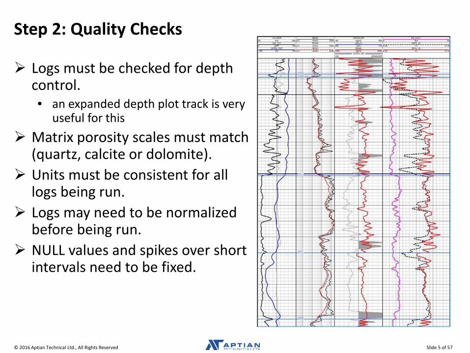
Step 2: Quality Checks
Logs must be checked for depth control. • an expanded depth plot track is very
useful for this Matrix porosity scales must match
(quartz, calcite or dolomite). Units must be consistent for all
logs being run. Logs may need to be normalized
before being run. NULL values and spikes over short
intervals need to be fixed.
© 2016 Aptian Technical Ltd., All Rights Reserved Slide 6 of 57
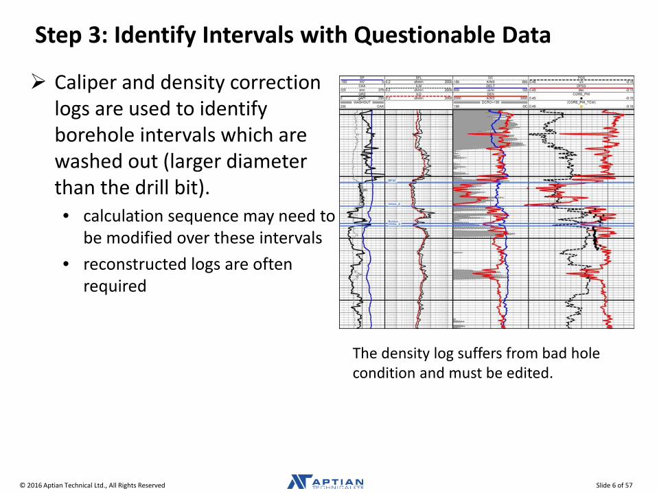
Step 3: Identify Intervals with Questionable Data
Caliper and density correction logs are used to identify borehole intervals which are washed out (larger diameter than the drill bit). • calculation sequence may need to
be modified over these intervals • reconstructed logs are often
required
The density log suffers from bad hole condition and must be edited.
© 2016 Aptian Technical Ltd., All Rights Reserved Slide 7 of 57
Step 4: Calculate Volume Shale
Petrophysicists define volume shale as the bulk volume of the rock composed of clay minerals and clay bound water.
Gamma ray log is typically used to calculate shale volume. • A non-linear relationship between shale and clean endpoints is required for
radioactive intervals (Clavier, etc.). A spectral gamma ray log is the most useful for determining shale volume
over radioactive intervals. • thorium, potassium and uranium
o thorium is associated with clay o potassium is associated with feldspar o uranium is associated with organics
Volume shale can also be calculated from the SP log, resistivity log, and separation between neutron and density logs.
Results should be calibrated to core or cutting data whenever possible. • clay volume from XRD
© 2016 Aptian Technical Ltd., All Rights Reserved Slide 8 of 57
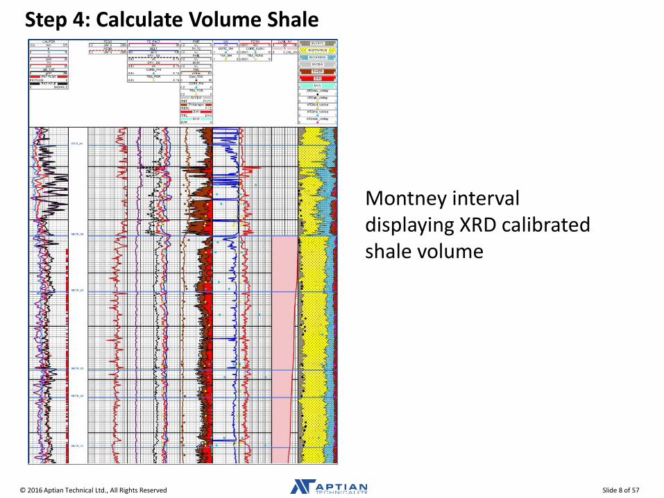
Step 4: Calculate Volume Shale
Montney interval displaying XRD calibrated shale volume
© 2016 Aptian Technical Ltd., All Rights Reserved Slide 9 of 57
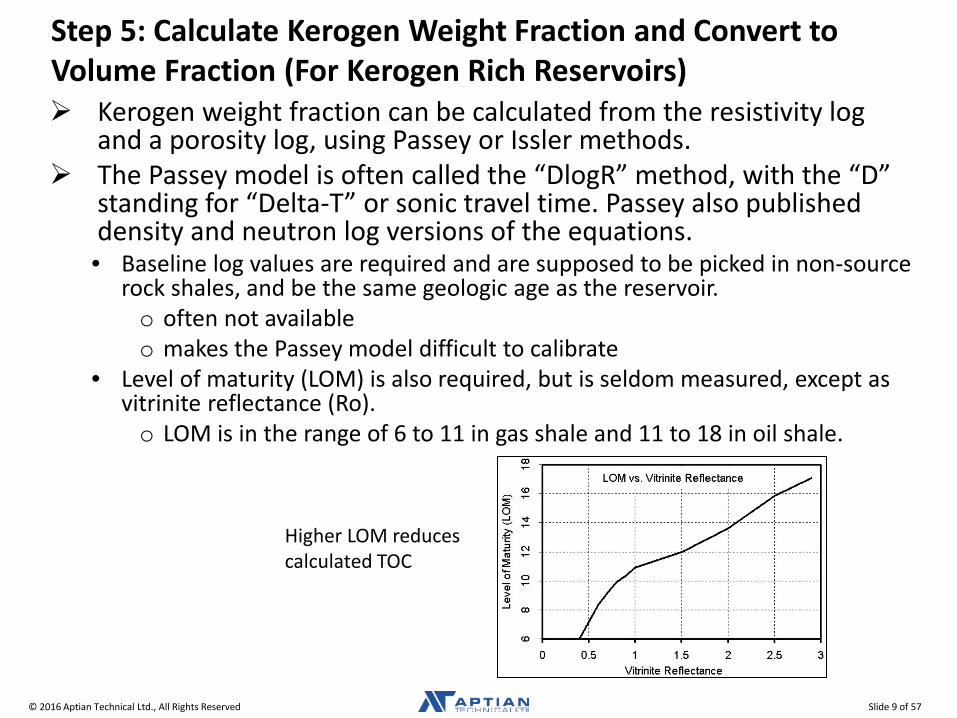
Step 5: Calculate Kerogen Weight Fraction and Convert to Volume Fraction (For Kerogen Rich Reservoirs) Kerogen weight fraction can be calculated from the resistivity log
and a porosity log, using Passey or Issler methods. The Passey model is often called the “DlogR” method, with the “D”
standing for “Delta-T” or sonic travel time. Passey also published density and neutron log versions of the equations. • Baseline log values are required and are supposed to be picked in non-source
rock shales, and be the same geologic age as the reservoir. o often not available o makes the Passey model difficult to calibrate
• Level of maturity (LOM) is also required, but is seldom measured, except as vitrinite reflectance (Ro). o LOM is in the range of 6 to 11 in gas shale and 11 to 18 in oil shale.
Higher LOM reduces calculated TOC
© 2016 Aptian Technical Ltd., All Rights Reserved Slide 10 of 57
Step 5: Calculate Kerogen Weight Fraction and Convert to Volume Fraction (For Kerogen Rich Reservoirs)
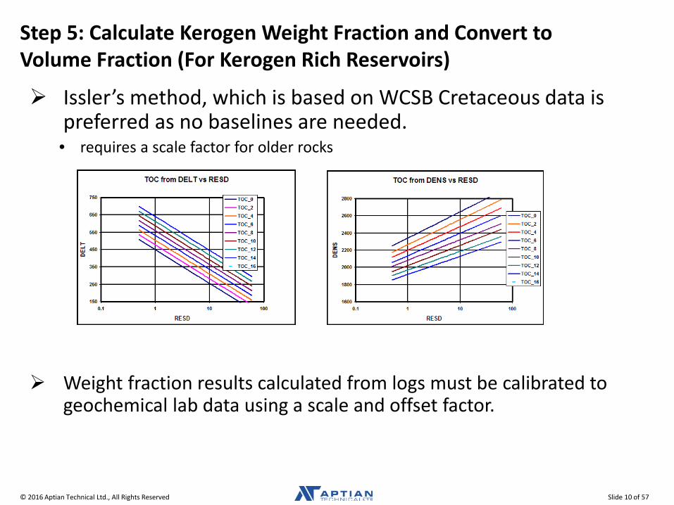
Issler’s method, which is based on WCSB Cretaceous data is preferred as no baselines are needed. • requires a scale factor for older rocks
Weight fraction results calculated from logs must be calibrated to geochemical lab data using a scale and offset factor.
© 2016 Aptian Technical Ltd., All Rights Reserved Slide 11 of 57
Step 5: Calculate Kerogen Weight Fraction and Convert to Volume Fraction (For Kerogen Rich Reservoirs)
Kerogen volume is calculated by converting TOC weight fraction. • lab TOC measures only the carbon content in the kerogen
o kerogen also contains oxygen, nitrogen, sulphur, etc. • conversion factor is the ratio of carbon weight to total kerogen weight
o typical range is from 0.68 to 0.95, with most common near 0.80
Kerogen mass fraction is then converted to volume fraction using a density in the range of 1200 to 1400 kg/m3.
© 2016 Aptian Technical Ltd., All Rights Reserved Slide 12 of 57
Step 5: Calculate Kerogen Weight Fraction and Convert to Volume Fraction (For Kerogen Rich Reservoirs)
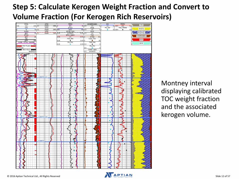
Montney interval displaying calibrated TOC weight fraction and the associated kerogen volume.
© 2016 Aptian Technical Ltd., All Rights Reserved Slide 13 of 57
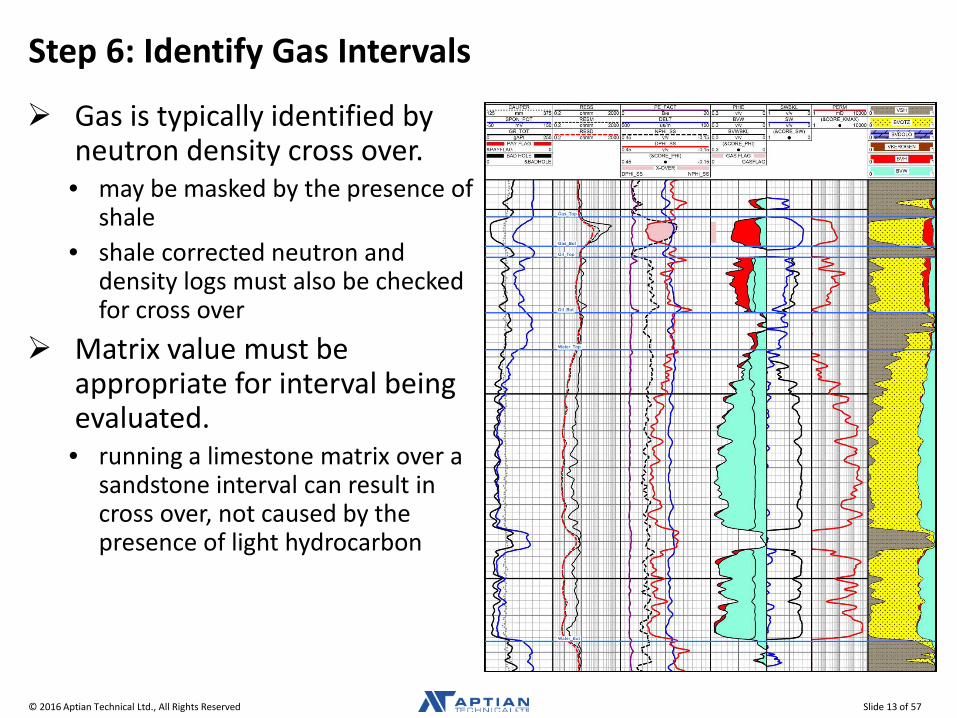
Step 6: Identify Gas Intervals
Gas is typically identified by neutron density cross over. • may be masked by the presence of
shale • shale corrected neutron and
density logs must also be checked for cross over
Matrix value must be appropriate for interval being evaluated. • running a limestone matrix over a
sandstone interval can result in cross over, not caused by the presence of light hydrocarbon
© 2016 Aptian Technical Ltd., All Rights Reserved Slide 14 of 57
Step 7: Identify Coal, Salt and Anhydrite Intervals
Coal intervals are identified by high neutron and density porosity log readings. • usually have fairly low GR reading, but not always • usually washed out
Salt is identified by low GR readings, along with a bulk density reading close to 2000 kg/m3, and a neutron porosity close to zero. • sonic log will read 220 us/m over salt intervals
Anhydrite is identified by low GR readings, along with a bulk density reading close to 2980 kg/m3, and a neutron porosity value close to zero.
© 2016 Aptian Technical Ltd., All Rights Reserved Slide 15 of 57
Step 8: Calculate Total Porosity
Total porosity includes clay bound water (CBW). • kerogen will also look like porosity to conventional logs
Porosity from the neutron density cross plot method is the preferred approach. • relatively independent of grain density changes
Other porosity models may also be used. • neutron sonic cross plot (less sensitive to bad bore hole conditions) • density only (very sensitive to changes in grain density and bore hole
conditions) • sonic only (very sensitive to changes in matrix travel time) • neutron only (not recommended, a last resort)
© 2016 Aptian Technical Ltd., All Rights Reserved Slide 16 of 57
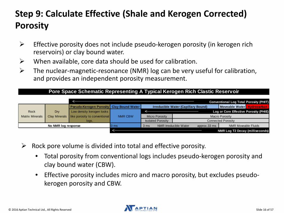
Step 9: Calculate Effective (Shale and Kerogen Corrected) Porosity
Effective porosity does not include pseudo-kerogen porosity (in kerogen rich reservoirs) or clay bound water.
When available, core data should be used for calibration. The nuclear-magnetic-resonance (NMR) log can be very useful for calibration,
and provides an independent porosity measurement.
Rock pore volume is divided into total and effective porosity. • Total porosity from conventional logs includes pseudo-kerogen porosity and
clay bound water (CBW). • Effective porosity includes micro and macro porosity, but excludes pseudo-
kerogen porosity and CBW.
Pseudo-Kerogen Porosity Clay Bound Water Moveable Water HydrocarbonRock Dry Low density kerogen looks
Matrix Minerals Clay Minerals like porosity to conventional NMR CBWlogs.
0 ms 3 ms approx.33 ms
Pore Space Schematic Representing A Typical Kerogen Rich Clastic Reservoir
NMR Log T2 Decay (milliseconds)
Conventional Log Total Porosity (PHIT)
No NMR log response
Irreducible Water (Capillary Bound)
Macro PorosityConnected Porosity
NMR Moveable FluidsNMR Irreducible Water
Micro PorosityIsolated Porosity
Log or Core Effective Porosity (PHIE)
© 2016 Aptian Technical Ltd., All Rights Reserved Slide 17 of 57
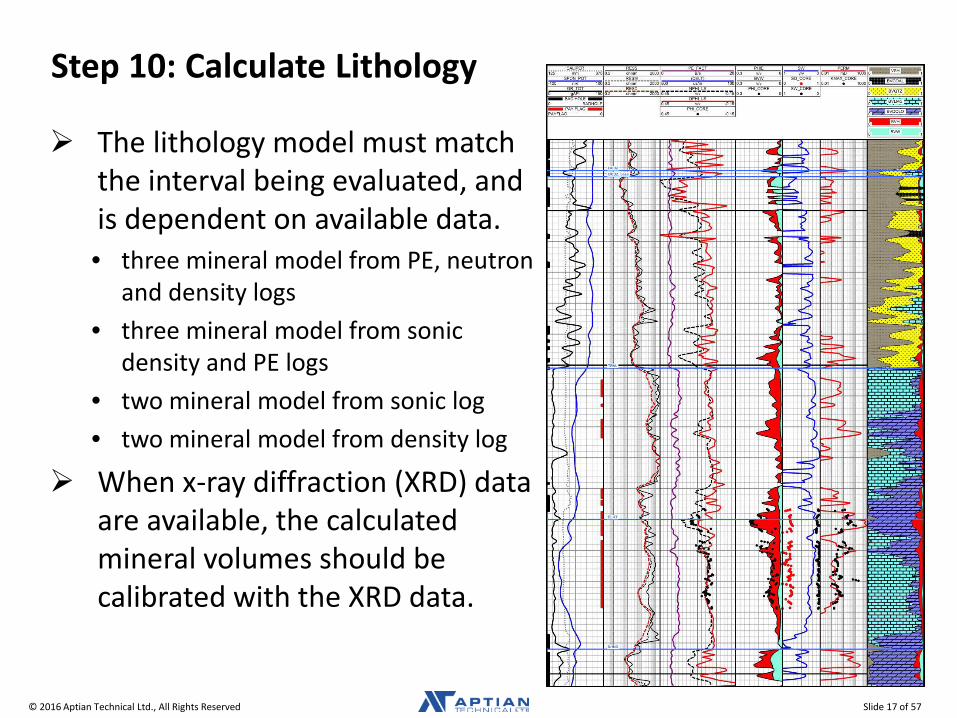
Step 10: Calculate Lithology
The lithology model must match the interval being evaluated, and is dependent on available data. • three mineral model from PE, neutron
and density logs • three mineral model from sonic
density and PE logs • two mineral model from sonic log • two mineral model from density log
When x-ray diffraction (XRD) data are available, the calculated mineral volumes should be calibrated with the XRD data.
© 2016 Aptian Technical Ltd., All Rights Reserved Slide 18 of 57
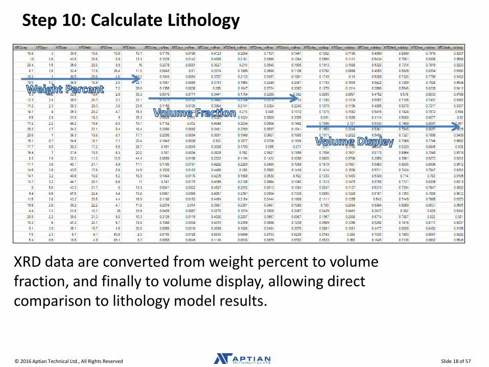
Step 10: Calculate Lithology
XRD data are converted from weight percent to volume fraction, and finally to volume display, allowing direct comparison to lithology model results.
© 2016 Aptian Technical Ltd., All Rights Reserved Slide 19 of 57
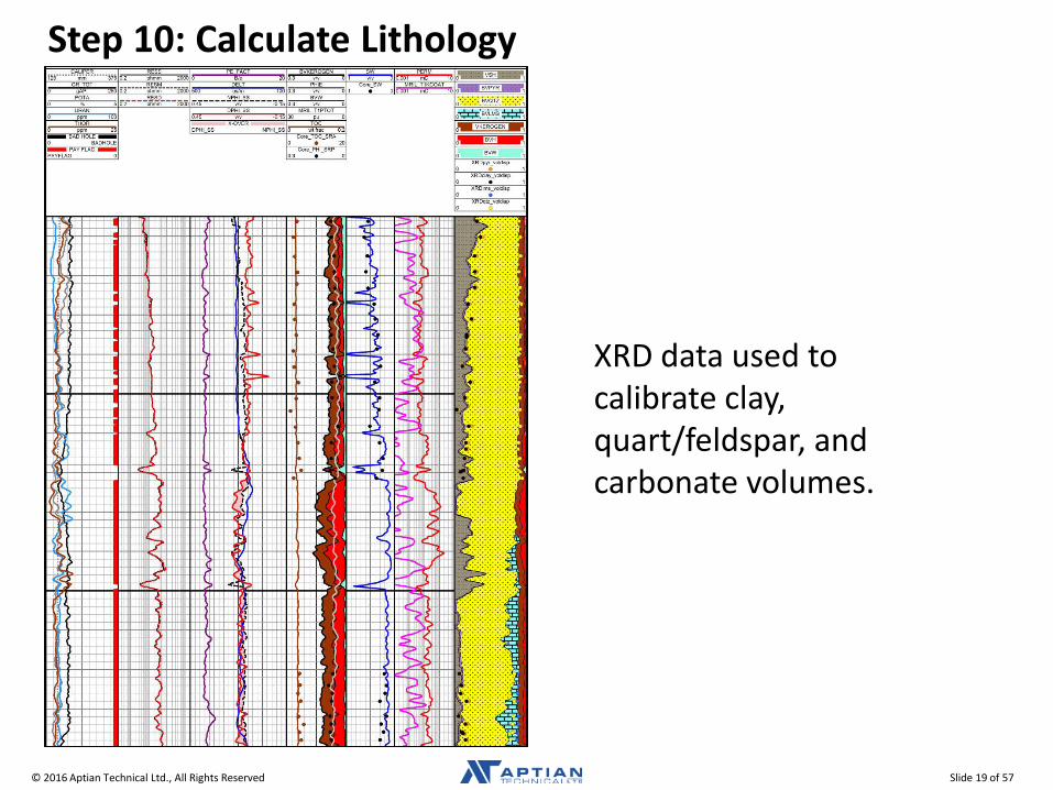
Step 10: Calculate Lithology
XRD data used to calibrate clay, quart/feldspar, and carbonate volumes.
© 2016 Aptian Technical Ltd., All Rights Reserved Slide 20 of 57
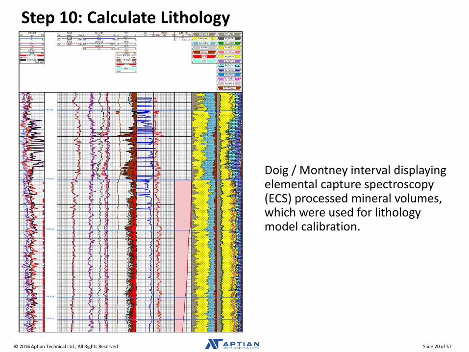
Step 10: Calculate Lithology
Doig / Montney interval displaying elemental capture spectroscopy (ECS) processed mineral volumes, which were used for lithology model calibration.
© 2016 Aptian Technical Ltd., All Rights Reserved Slide 21 of 57
Step 11: Calculate Water Saturation
The modified Simandoux equation works well for most situations. • accounts for low resistivity shale • reduces to the Archie equation when volume shale equals zero • better behaved in low porosity than most other models
o Dual water models may also work, but may give silly results when volume shale is high or porosity is very low.
Tortuosity, cementation and saturation exponents (a, m and n) are required inputs.
• In many cases electrical properties must be varied from world averages to get SW to match lab data. o A = 1.0 o M = N = 1.5 to 1.8 o lab measurement of electrical properties is essential
Rw at reference temperature is required and must be corrected to formation temperature.
• shale resistivity is required • A deep resistivity log reading and accurate porosity are also required.
Calibration can be done with core SW or capillary pressure data. • Both pose problems in unconventional reservoirs, especially reservoirs with thin
porosity laminations. • common sense may have to prevail over “facts”
© 2016 Aptian Technical Ltd., All Rights Reserved Slide 22 of 57
Step 12: Calculate Permeability Index The Wylie-Rose equation works well in low porosity reservoirs.
• calibration constant can range between 100,000 to 150,000 and beyond o adjusted to get a good match to conventional core permeability data
• generally assume the calculated SW is also the irreducible SW o this assumption may not always be correct
An exponential equation derived from regression of core permeability against core porosity may also work well. • Perm = 10^(A1*PHIE+A2)
o typical values for A1 and A2 are 20.0 and -3.0 respectively o High perm data caused by micro or macro fractures should be eliminated
before performing the regression. Other permeability models are often used.
• Coates-Denoo • power law model • Lucia rock fabric model
These models match conventional core permeability quite well, but will not match permeability derived from crushed samples using the GRI protocol.
Permeability index must be corrected to in-situ conditions. • flow capacity from a well test can be used for calibration
© 2016 Aptian Technical Ltd., All Rights Reserved Slide 23 of 57
Step 13: Net Reservoir and Net Pay
In many shale gas and some shale oil plays, typical porosity cutoffs for net reservoir are very low. • 2 or 3% for those with an optimistic view • 4 or 5% for the pessimistic view
The water saturation cutoff for net pay is quite variable. • Some unconventional reservoirs have very little water in the free
porosity so the SW cutoff is not too important. • Others have higher apparent water saturation than might be expected
for a productive reservoir. However, they do produce, so the SW cutoff must be quite liberal.
• SW cutoffs between 50 and 80% are common
Shale volume cutoffs are usually quite liberal for unconventional reservoirs, and are usually set above the 50% mark. • Multiple cutoff sets help assess the sensitivity to arbitrary choices
• gives an indication of the risk or variability in OGIP or OOIP
© 2016 Aptian Technical Ltd., All Rights Reserved Slide 24 of 57
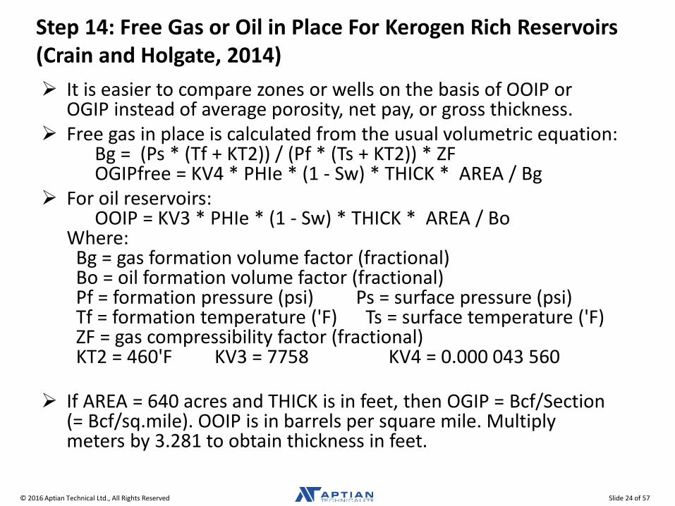
Step 14: Free Gas or Oil in Place For Kerogen Rich Reservoirs (Crain and Holgate, 2014) It is easier to compare zones or wells on the basis of OOIP or
OGIP instead of average porosity, net pay, or gross thickness. Free gas in place is calculated from the usual volumetric equation:
Bg = (Ps * (Tf + KT2)) / (Pf * (Ts + KT2)) * ZF OGIPfree = KV4 * PHIe * (1 - Sw) * THICK * AREA / Bg
For oil reservoirs: OOIP = KV3 * PHIe * (1 - Sw) * THICK * AREA / Bo Where: Bg = gas formation volume factor (fractional) Bo = oil formation volume factor (fractional) Pf = formation pressure (psi) Ps = surface pressure (psi) Tf = formation temperature ('F) Ts = surface temperature ('F) ZF = gas compressibility factor (fractional) KT2 = 460'F KV3 = 7758 KV4 = 0.000 043 560
If AREA = 640 acres and THICK is in feet, then OGIP = Bcf/Section (= Bcf/sq.mile). OOIP is in barrels per square mile. Multiply meters by 3.281 to obtain thickness in feet.
© 2016 Aptian Technical Ltd., All Rights Reserved Slide 25 of 57
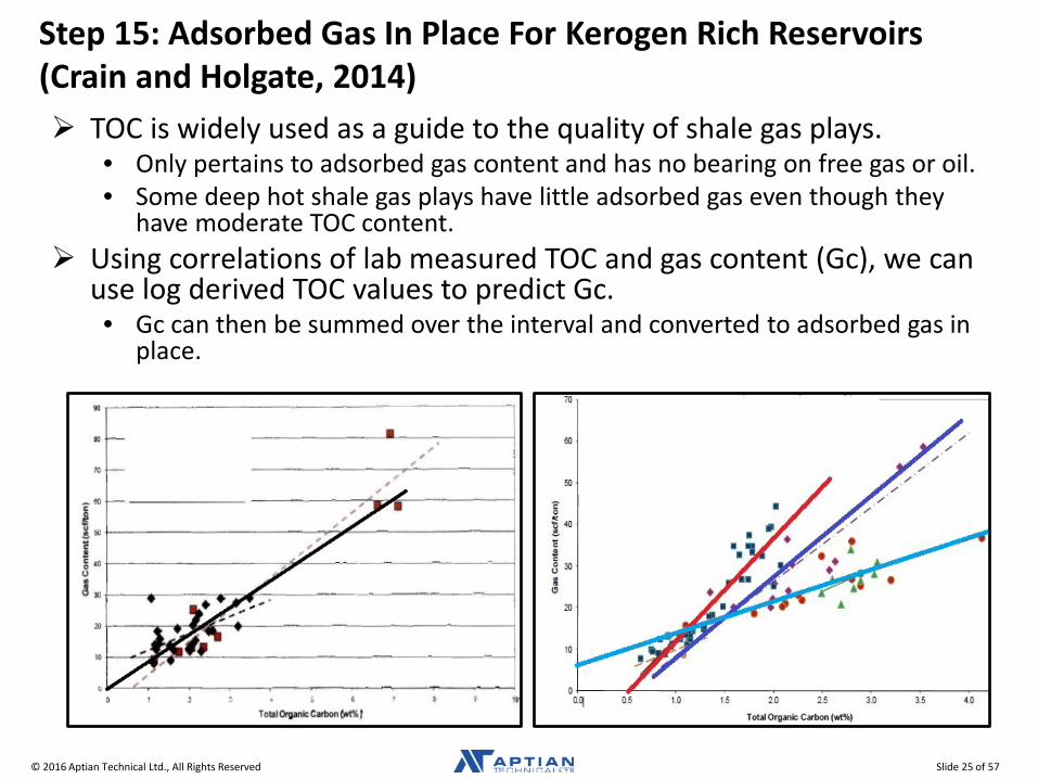
Step 15: Adsorbed Gas In Place For Kerogen Rich Reservoirs (Crain and Holgate, 2014) TOC is widely used as a guide to the quality of shale gas plays.
• Only pertains to adsorbed gas content and has no bearing on free gas or oil. • Some deep hot shale gas plays have little adsorbed gas even though they
have moderate TOC content. Using correlations of lab measured TOC and gas content (Gc), we can
use log derived TOC values to predict Gc. • Gc can then be summed over the interval and converted to adsorbed gas in
place.
© 2016 Aptian Technical Ltd., All Rights Reserved Slide 26 of 57
Step 16: Reconstruct Sonic and Density Log Curves (Crain and Holgate, 2013)
For stimulation design modeling, the logs should represent a water filled reservoir. • Since logs read the invaded zone, light hydrocarbons (light oil or gas) make the
density log read too low and the sonic log read too high, compared to the water filled case.
Sonic data are also affected by one or several of the following: • fractures, laminations • TOC • external stress and temperature • borehole conditions • pore pressure
Rock mechanical properties are calculated based on reconstructed logs derived from the petrophysical analysis. • for use in stimulation design programs
The reconstructed logs eliminate gas effect (if any) and low quality data caused by rough borehole.
© 2016 Aptian Technical Ltd., All Rights Reserved Slide 27 of 57
Step 16: Reconstruct Sonic and Density Log Curves
( ) ( )[ ] ( ) txoffptvhoffptvvobtvc EPDPDDP σεγαγαγν
ν+++++−
−=
1
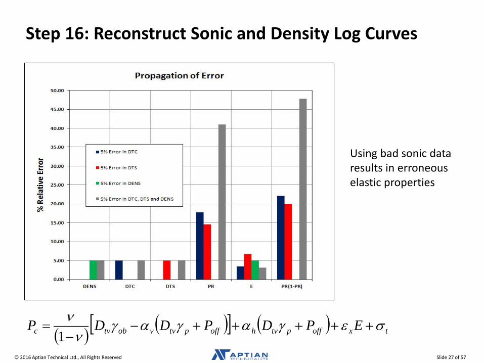
Using bad sonic data results in erroneous elastic properties
© 2016 Aptian Technical Ltd., All Rights Reserved Slide 28 of 57
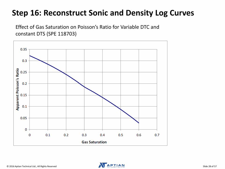
Effect of Gas Saturation on Poisson’s Ratio for Variable DTC and constant DTS (SPE 118703)
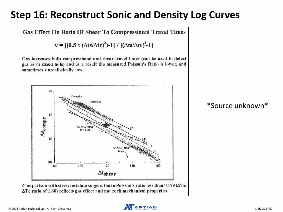
Step 16: Reconstruct Sonic and Density Log Curves
© 2016 Aptian Technical Ltd., All Rights Reserved Slide 29 of 57
Step 16: Reconstruct Sonic and Density Log Curves
*Source unknown*
© 2016 Aptian Technical Ltd., All Rights Reserved Slide 30 of 57
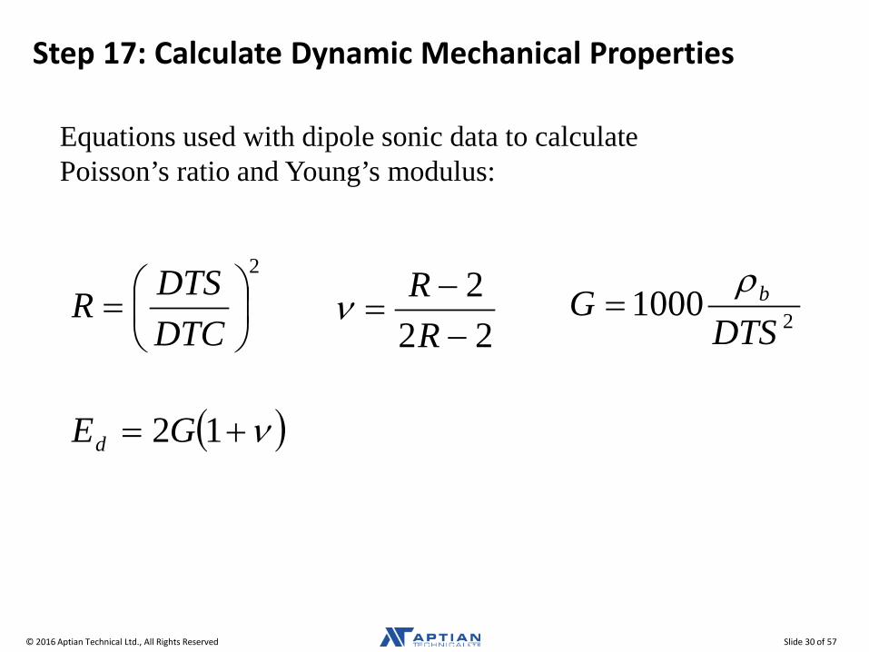
Equations used with dipole sonic data to calculate Poisson’s ratio and Young’s modulus:
2
=
DTCDTSR
222−−
=R
Rν 21000DTS
G bρ=
( )ν+= 12GEd
Step 17: Calculate Dynamic Mechanical Properties
© 2016 Aptian Technical Ltd., All Rights Reserved Slide 31 of 57
Step 17: Calculate Dynamic Mechanical Properties
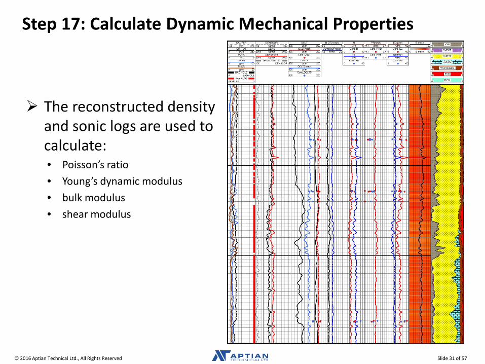
The reconstructed density and sonic logs are used to calculate: • Poisson’s ratio • Young’s dynamic modulus • bulk modulus • shear modulus
© 2016 Aptian Technical Ltd., All Rights Reserved Slide 32 of 57
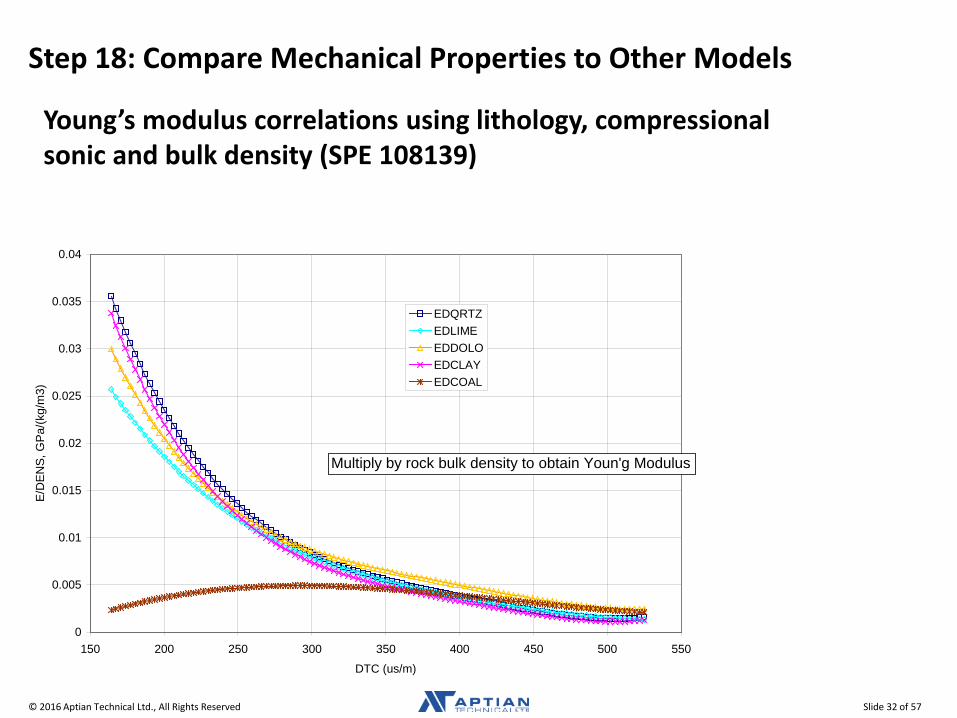
Young’s modulus correlations using lithology, compressional sonic and bulk density (SPE 108139)
0
0.005
0.01
0.015
0.02
0.025
0.03
0.035
0.04
150 200 250 300 350 400 450 500 550
DTC (us/m)
E/D
ENS,
GPa
/(kg/
m3)
EDQRTZEDLIMEEDDOLOEDCLAYEDCOAL
Multiply by rock bulk density to obtain Youn'g Modulus
Step 18: Compare Mechanical Properties to Other Models
© 2016 Aptian Technical Ltd., All Rights Reserved Slide 33 of 57
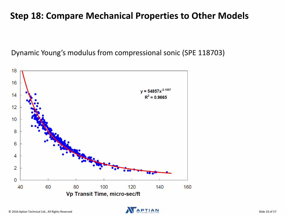
Step 18: Compare Mechanical Properties to Other Models
Dynamic Young’s modulus from compressional sonic (SPE 118703)
© 2016 Aptian Technical Ltd., All Rights Reserved Slide 34 of 57
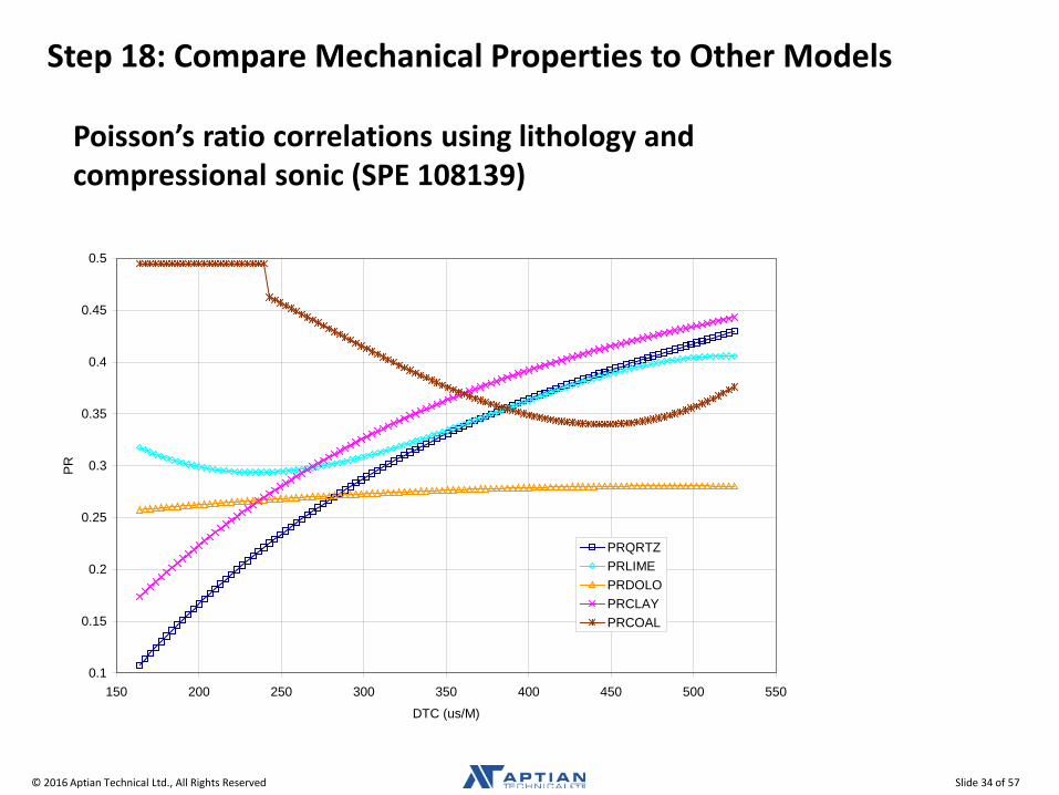
Poisson’s ratio correlations using lithology and compressional sonic (SPE 108139)
0.1
0.15
0.2
0.25
0.3
0.35
0.4
0.45
0.5
150 200 250 300 350 400 450 500 550
DTC (us/M)
PR
PRQRTZPRLIMEPRDOLOPRCLAYPRCOAL
Step 18: Compare Mechanical Properties to Other Models
© 2016 Aptian Technical Ltd., All Rights Reserved Slide 35 of 57
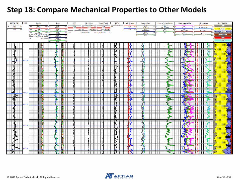
Step 18: Compare Mechanical Properties to Other Models
© 2016 Aptian Technical Ltd., All Rights Reserved Slide 36 of 57
Step 18: Compare Mechanical Properties to Other Models empirically developed rock tables (SPE 86989) Mutilinear regression models can also be used with corrected
log data. • ED(GR, RHOB, NPHI, …) • PR(GR, RHOB, NPHI, …)
Simple linear relationships may work well in clastic intervals. • ED(VSH) • PR(VSH)
Neural Network models may also work with corrected log data.

© 2016 Aptian Technical Ltd., All Rights Reserved Slide 37 of 57
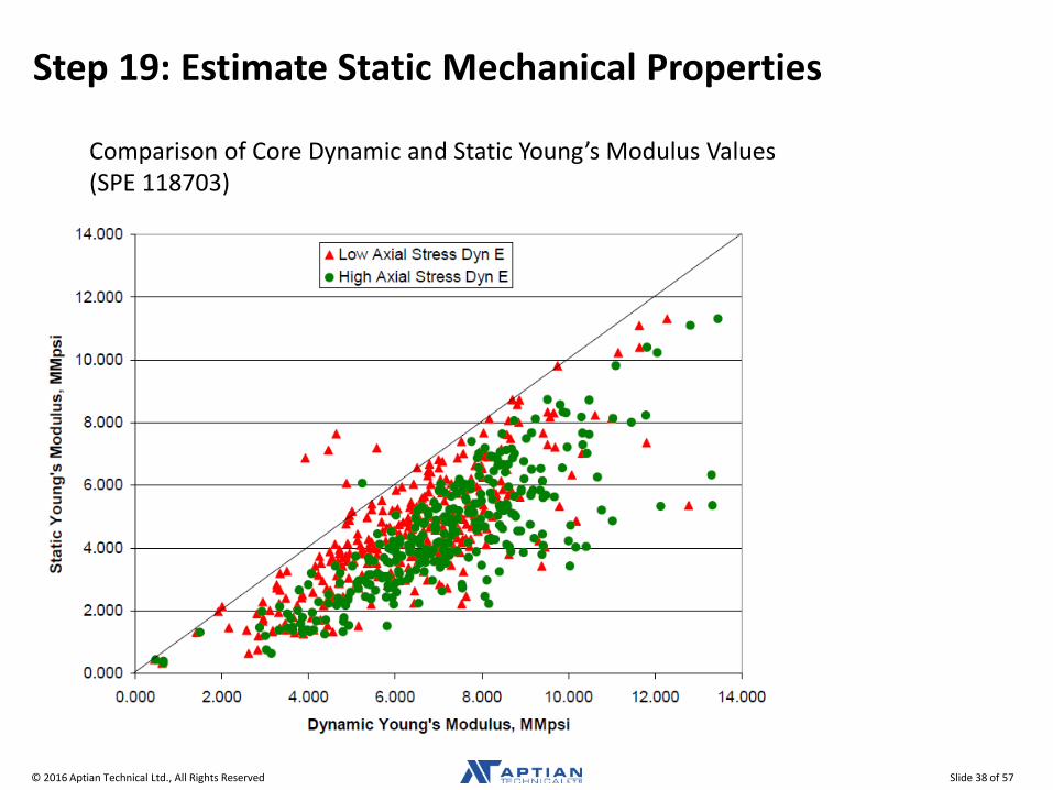
Step 19: Estimate Static Mechanical Properties Static values differ from dynamic values because strain and strain
rate are dependent on the measurement method. • dynamic: acoustic wave propagation is a phenomenon of small strain at a
large strain rate • static (triaxial): large strain at small strain rate
Rocks appear stiffer in response to an elastic wave, compared to a rock mechanics laboratory (triaxial) test. • the weaker the rock, the larger the difference • accounts for the difference between dynamic and static Young’s moduli
The difference between dynamic and static Poisson’s ratio is very small, and is generally not considered.
Static mechanical rock properties are needed as input for hydraulic fracture simulation work. • Static values more closely represent the strain and strain rate created
during hydraulic frac stimulation treatments. • many transforms have been published
© 2016 Aptian Technical Ltd., All Rights Reserved Slide 38 of 57
Step 19: Estimate Static Mechanical Properties
Comparison of Core Dynamic and Static Young’s Modulus Values (SPE 118703)
© 2016 Aptian Technical Ltd., All Rights Reserved Slide 39 of 57
Step 19: Estimate Static Mechanical Properties
Lacy’s equations also work well for estimating static modulus from dynamic modulus (SPE 38716).
• The lithology dependent correlations can be combined using bulk volumes from petrophysical analysis.
Brittleness index • dependent on static Young’s modulus and Poisson’s ratio (rock stiffness) • SPE 115258 works well
© 2016 Aptian Technical Ltd., All Rights Reserved Slide 40 of 57
Step 20: Calculate and Calibrate Closure Stress
( ) ( )[ ] ( ) txoffptvhoffptvvobtvc EPDPDDP σεγαγαγν
ν+++++−
−=
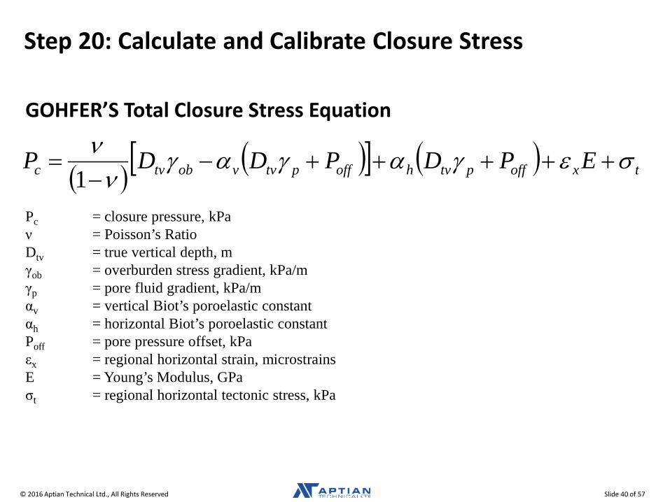
1Pc = closure pressure, kPa ν = Poisson’s Ratio Dtv = true vertical depth, m γob = overburden stress gradient, kPa/m γp = pore fluid gradient, kPa/m αv = vertical Biot’s poroelastic constant αh = horizontal Biot’s poroelastic constant Poff = pore pressure offset, kPa εx = regional horizontal strain, microstrains E = Young’s Modulus, GPa σt = regional horizontal tectonic stress, kPa
GOHFER’S Total Closure Stress Equation
© 2016 Aptian Technical Ltd., All Rights Reserved Slide 41 of 57
Closure stress is calculated using GOHFER’S Total Stress equation and must be calibrated to local field conditions with a strain or stress correction factor.
In tectonically active areas, the closure stress calculated from logs will be too low and will need to be increased. • εx= regional horizontal strain • σt = regional horizontal tectonic stress • generally, the strain offset approach is favoured
The best way to calibrate closure stress is to review fracturing work, or perform a minifrac.
If possible, this step should be completed by the completion engineer (the person running the hydraulic frac simulation software).
Step 20: Calculate and Calibrate Closure Stress
© 2016 Aptian Technical Ltd., All Rights Reserved Slide 42 of 57
Step 20: Calculate and Calibrate Closure Stress
The density log is used to calculate overburden stress. Before the density log can be used, abnormally low data caused by bad hole, coal, etc. must be removed.
The easiest way to calculate overburden stress is by determining the average bulk density above treatment depth. • Bad density data are first eliminated by running a discriminator.
o caliper and density correction logs are typically used • With the discriminator applied, the average bulk density is calculated and then
used to calculate overburden stress. The more complicated approach requires integration of the bulk density
log. • This approach requires a synthetic density log to be created. The synthetic log
is then integrated from treatment depth to shallowest log reading. o still requires a bulk density value to be assigned from surface to
shallowest log reading The averaging method has proven to work very well, as long as the bad
quality density data are removed.
Overburden Stress
© 2016 Aptian Technical Ltd., All Rights Reserved Slide 43 of 57
Step 20: Calculate and Calibrate Closure Stress
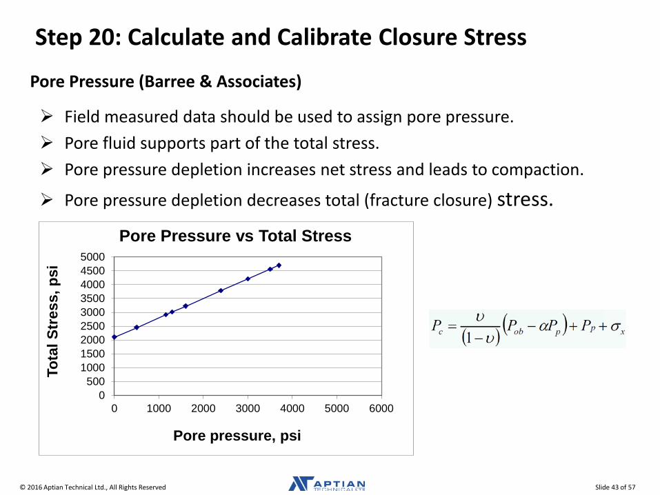
Field measured data should be used to assign pore pressure. Pore fluid supports part of the total stress. Pore pressure depletion increases net stress and leads to compaction.
Pore pressure depletion decreases total (fracture closure) stress.
Pore Pressure (Barree & Associates)
0500
100015002000250030003500400045005000
0 1000 2000 3000 4000 5000 6000
Tota
l Str
ess,
psi
Pore pressure, psi
Pore Pressure vs Total Stress
© 2016 Aptian Technical Ltd., All Rights Reserved Slide 44 of 57
Step 20: Calculate and Calibrate Closure Stress
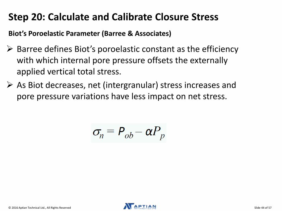
Barree defines Biot’s poroelastic constant as the efficiency with which internal pore pressure offsets the externally applied vertical total stress.
As Biot decreases, net (intergranular) stress increases and pore pressure variations have less impact on net stress.
Biot’s Poroelastic Parameter (Barree & Associates)
© 2016 Aptian Technical Ltd., All Rights Reserved Slide 45 of 57
0
0.1
0.2
0.3
0.4
0.5
0.6
0.7
0.8
0.9
1
0 0.05 0.1 0.15 0.2 0.25 0.3 0.35 0.4
Effective Porosity, fraction
Biot
's P
oroe
last
ic C
onst
ant
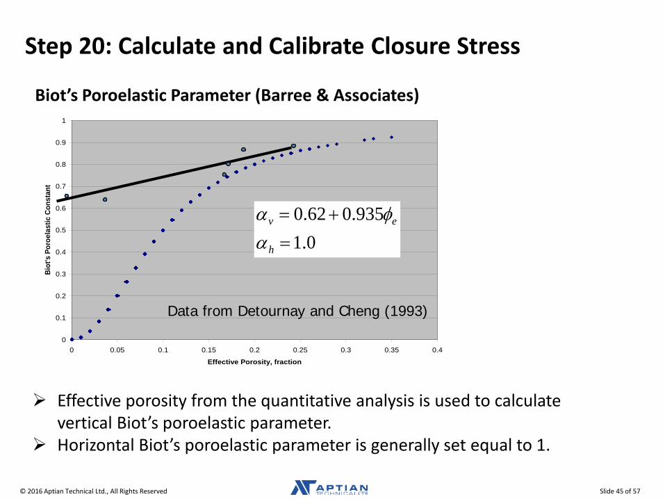
Data from Detournay and Cheng (1993)
0.1935.062.0
=+=
h
ev
αφα
Step 20: Calculate and Calibrate Closure Stress
Effective porosity from the quantitative analysis is used to calculate vertical Biot’s poroelastic parameter.
Horizontal Biot’s poroelastic parameter is generally set equal to 1.
Biot’s Poroelastic Parameter (Barree & Associates)
© 2016 Aptian Technical Ltd., All Rights Reserved Slide 46 of 57
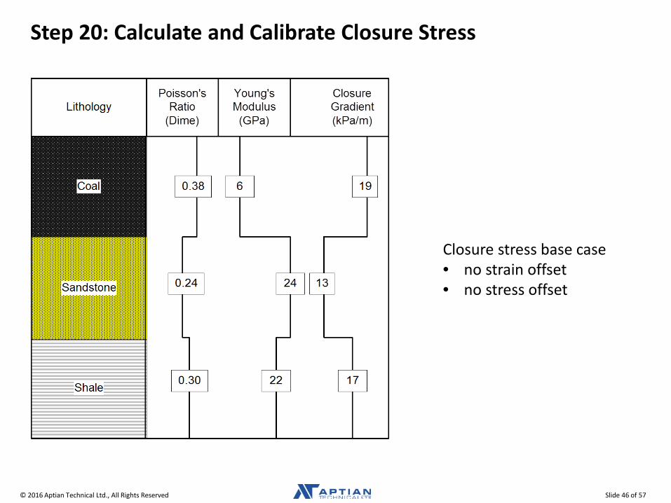
Step 20: Calculate and Calibrate Closure Stress
Closure stress base case • no strain offset • no stress offset
© 2016 Aptian Technical Ltd., All Rights Reserved Slide 47 of 57
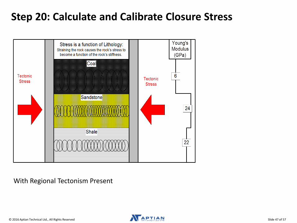
Step 20: Calculate and Calibrate Closure Stress
With Regional Tectonism Present
© 2016 Aptian Technical Ltd., All Rights Reserved Slide 48 of 57
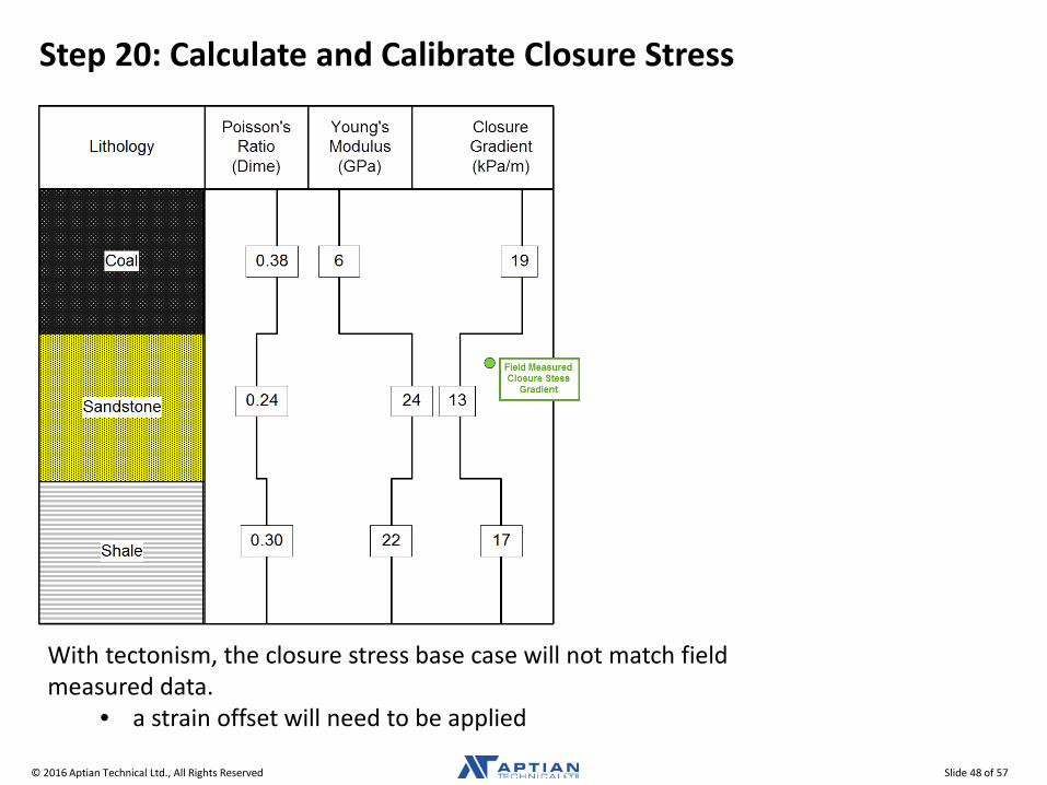
Step 20: Calculate and Calibrate Closure Stress
With tectonism, the closure stress base case will not match field measured data.
• a strain offset will need to be applied
© 2016 Aptian Technical Ltd., All Rights Reserved Slide 49 of 57
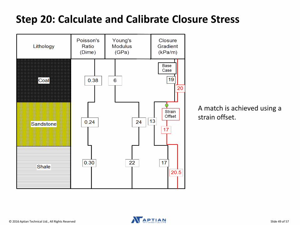
Step 20: Calculate and Calibrate Closure Stress
A match is achieved using a strain offset.
© 2016 Aptian Technical Ltd., All Rights Reserved Slide 50 of 57
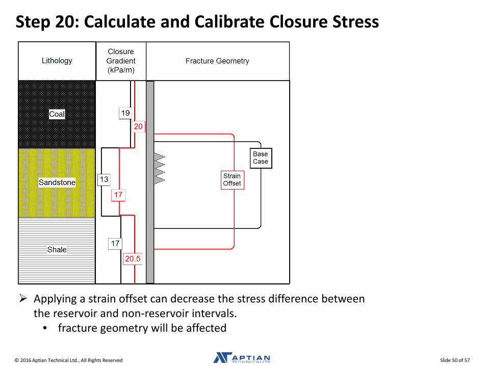
Step 20: Calculate and Calibrate Closure Stress
Applying a strain offset can decrease the stress difference between the reservoir and non-reservoir intervals.
• fracture geometry will be affected
© 2016 Aptian Technical Ltd., All Rights Reserved Slide 51 of 57
Examples
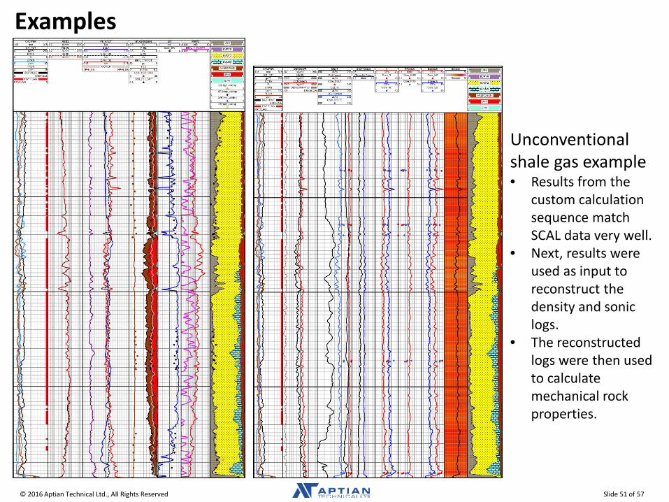
Unconventional shale gas example • Results from the
custom calculation sequence match SCAL data very well.
• Next, results were used as input to reconstruct the density and sonic logs.
• The reconstructed logs were then used to calculate mechanical rock properties.
© 2016 Aptian Technical Ltd., All Rights Reserved Slide 52 of 57
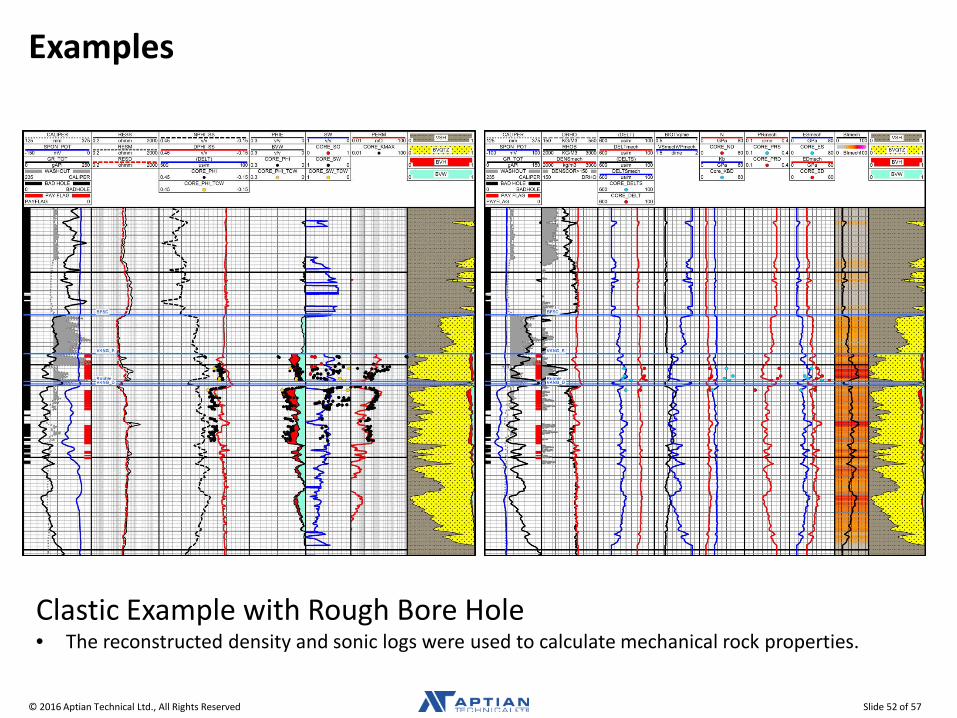
Examples
Clastic Example with Rough Bore Hole • The reconstructed density and sonic logs were used to calculate mechanical rock properties.
© 2016 Aptian Technical Ltd., All Rights Reserved Slide 53 of 57
Conclusions A three well minimum is recommended for all projects.
• Rarely will the subject well have all required data needed to complete a calibrated petrophysical analysis.
• Offset wells should always be reviewed and used to put together the best data set possible.
• The accuracy of the petrophysical model improves with an increased number of wells reviewed.
Trying to perform a petrophysical analysis with hydraulic frac simulation software is not recommended. • Robust petrophysical software and an experienced petrophysicist are required to
generate accurate mechanical rock properties. Closure stress calculation and calibration should, if possible, be carried out by
an experienced completion engineer. This step should be run within the hydraulic frac simulation software. • field data must be reviewed and used for calibration
o pore pressure o closure pressure
© 2016 Aptian Technical Ltd., All Rights Reserved Slide 54 of 57
Conclusions
Holgate and Crain’s 20 step petrophysical workflow has proven successful in many challenging reservoir environments, worldwide.
Sufficient time and talent should be allowed by management for the process.
The reconstruction step is particularly important for sonic and density logs. • small input errors amplify to become surprisingly large • Reconstructed logs should be used to calculate Young’s modulus and Poisson’s
ratio. o essential input to stimulation design software packages
A full suite of TOC and XRD mineralogy from samples, along with core porosity and saturation data, are needed to calibrate results from any petrophysical analysis of unconventional reservoirs. • bulk clay and TOC are the two critical lab measurements
© 2016 Aptian Technical Ltd., All Rights Reserved Slide 55 of 57
Conclusions Without valid calibration data, petrophysical analysis will have possible error
bars too large to allow meaningful financial decisions. Holgate and Crain’s deterministic workflow allows all available empirical data
to be used in a logical and consistent manner at each step to calibrate and refine results.
Petrophysical analysis results travel well beyond the initial need to know porosity and water saturation. • oil and gas in place • reservoir stimulation • placement of horizontal wells • financial reports
The cost of the full analysis and reconstruction is trivial compared to the cost of completion, or worse, an unsuccessful completion design.

© 2016 Aptian Technical Ltd., All Rights Reserved Slide 56 of 57
About The Authors
E. R. (Ross) Crain, P.Eng. is a Consulting Petrophysicist and Professional Engineer, with over 50 years of experience in reservoir description, petrophysical analysis, and management. He is a specialist in the integration of well log analysis and petrophysics with geophysical, geological, engineering, stimulation, and simulation phases of the oil and gas industry, with widespread Canadian and Overseas experience. He has authored more than 60 articles and technical papers. His online shareware textbook, Crain's Petrophysical Handbook, is widely used as a reference for practical petrophysical analysis methods. Mr. Crain is an Honorary Member and Past President of the Canadian Well Logging Society (CWLS), a Member of SPWLA, and a Registered Professional Engineer with APEGA. [email protected]
Dorian Holgate, P. Geol. is the principal consultant of Aptian Technical Limited, an independent petrophysical consulting practice. He graduated from the University of Calgary with a B.Sc. in Geology in 2000 and completed the Applied Geostatistics Citation program from the University of Alberta in 2007. After graduation, he began working in the field for BJ Services (now Baker Hughes) and completed BJ’s Associate Engineer Program. Later, he joined BJ’s Reservoir Services Group, applying the analysis of well logs to rock mechanics to optimize hydraulic fracturing programs. In 2005, Dorian joined Husky Energy as a Petrophysicist and progressed to an Area Geologist role. He completed a number of petrophysical studies and built 3-D geological models for carbonate and clastic reservoirs. Dorian is a Member of CSPG, SPE, SPWLA, CWLS, and a Registered Professional Geologist with APEGA. [email protected]
© 2016 Aptian Technical Ltd., All Rights Reserved Slide 57 of 57
References Barree, R.D., Gilbert, J.V. and Conway, M.W.”Stress and Rock Property Profiling for Unconventional
Reservoir Stimulation,” paper SPE 118703 presented at the 2009 SPE Hydraulic Fracturing Technology Conference held in the Woodlands, Texas, USA, 19-21 January 2009.
Crain, E.R., “Crain’s Petrophysical Handbook.”, at http://www.spec2000.net, Rocky Mountain House, Alberta, Canada, 2013.
Crain, E.R., and Holgate, Dorian. “Synthetic Log Curves: An Essential Ingredient For Successful Stimulation Design.” CSPG Reservoir Volume 40, Issue 5, May 2013: 19-24.
Crain, E.R., and Holgate, Dorian. “A 12 Step Program to Reduce Uncertainty in Kerogen-Rich Reservoirs: Part 1 – Getting the Right Porosity.” CSPG Reservoir Volume 41, Issue 3, March 2014: 19-23.
Crain, E.R., and Holgate, Dorian. “A 12 Step Program to Reduce Uncertainty in Kerogen-Rich Reservoirs: Part 2 – Getting the Right Hydrocarbon Volume.” CSPG Reservoir Volume 41, Issue 4, April 2014: 34-38.
Crain, E.R., and Holgate, Dorian. “Digital Log Data To Mechanical Rock Properties For Stimulation Design,” presented at the GeoConvention Conference held in Calgary, Alberta, Canada, 12-16 May 2014.
Lacy, L.L., “Dynamic Rock Mechanics Testing for Optimized Fracture Designs,” paper SPE 38716. Leshchyshyn, T.H., et. al., “Using Empirically Developed Rock Tables to Predict and History Match Fracture
Stimulations,” paper SPE 86989. Mullen, Mike., Roundtree, Russel., Barree, R.D., “A Composite Determination of Mechanical Rock
Properties for Stimulation Design (What To Do When You Don’t Have a Sonic Log),” paper SPE 108139. Rickman, Rick., and Mullen, Mike., et. al., “A Practical Use of Shale Petrophysics for Stimulation Design
Optimization: All Shale Plays Are Not Clones of the Barnett Shale,” paper SPE 115258.