Embed Size (px)
Citation preview
Linear Algebra and its Applications 424 (2007) 240–281www.elsevier.com/locate/laa
The higher-order derivatives of spectral functions �
Hristo S. Sendov
Department of Mathematics and Statistics, 50 Stone Road East, University of Guelph,Guelph, Ont., Canada N1G 2W1
Received 14 July 2006; accepted 20 December 2006Available online 19 January 2007
Submitted by R.A. Brualdi
Dedicated to Professor Roger Horn on the occasion of his 65th birthday
Abstract
We are interested in higher-order derivatives of functions of the eigenvalues of real symmetric matriceswith respect to the matrix argument. We describe a formula for the kth derivative of such functions in twogeneral cases.
The first case concerns the derivatives of the composition of an arbitrary (not necessarily symmetric)k-times differentiable function with the eigenvalues of symmetric matrices at a symmetric matrix with distincteigenvalues.
The second case describes the derivatives of the composition of a k-times differentiable separable sym-metric function with the eigenvalues of symmetric matrices at an arbitrary symmetric matrix. We showthat the formula significantly simplifies when the separable symmetric function is k-times continuouslydifferentiable.
As an application of the developed techniques, we re-derive the formula for the Hessian of a generalspectral function at an arbitrary symmetric matrix. The new tools lead to a shorter, cleaner derivation thanthe original one.
To make the exposition as self contained as possible, we have included the necessary background resultsand definitions. Proofs of the intermediate technical results are collected in the appendices.© 2007 Elsevier Inc. All rights reserved.
AMS classification: 49R50; 47A75
Keywords: Spectral function; Differentiable; Twice differentiable; Higher-order derivative; Eigenvalue optimization;Symmetric function; Perturbation theory; Tensor analysis; Hadamard product
� Research supported by NSERC.E-mail address: [email protected]
0024-3795/$ - see front matter ( 2007 Elsevier Inc. All rights reserved.doi:10.1016/j.laa.2006.12.013

H.S. Sendov / Linear Algebra and its Applications 424 (2007) 240–281 241
1. Introduction
We say that a real-valued function F of a real symmetric matrix argument is spectral if
F(UXUT) = F(X)
for every real symmetric matrix X in its domain and every orthogonal matrix U . That is, F(X) =F(Y ) if X and Y are symmetric and similar. The restriction of F to the subspace of diagonal matri-ces defines a function f (x) = F(Diag x) on a vector argument x ∈ Rn. The function f : Rn → R
is symmetric, that is, has the property
f (x) = f (Px) for any permutation matrix P and any x in the domain of f,
and in addition, F(X) = (f ◦ λ)(X), in which the eigenvalue map
λ(X) = (λ1(X), . . . , λn(X))
is the vector of eigenvalues of X arranged in non-increasing order.What smoothness properties of the symmetric function f are inherited by F ? The eigenvalue
map λ(X) is continuous but not always differentiable with respect to X. Even in domains whereλ(X) is differentiable, it is difficult to organize the differentiation process so that one arrives atan elegant formula for the higher-order derivatives of (f ◦ λ)(X).
An important subclass of spectral functions is obtained when f (x) = g(x1) + · · · + g(xn)
for some function g of one real variable. We call such symmetric functions separable; theircorresponding spectral functions are called separable spectral functions.
In [13] there is an explicit formulae for the gradient of the spectral function F in terms of thederivatives of the symmetric function f :
∇(f ◦ λ)(X) = V (Diag ∇f (λ(X)))V T, (1)
where V is any orthogonal matrix such that X = V (Diag λ(X))V T is the ordered spectral decom-position of X. In [17] a formula for the Hessian of F was given, whose structure appeared quitedifferent from the one for the gradient. Calculating the third and higher-order derivatives of F
becomes unmanageable without an appropriate language for describing them.In this work we generalize the work in [13,17] by proving, in two general cases, the following
formula for the kth derivative of a spectral function
∇k(f ◦ λ)(X) = V
⎛⎝∑σ∈P k
DiagσAσ (λ(X))
⎞⎠V T, (2)
where again X = V (Diag λ(X))V T. The sum is taken over all permutations on k elements, whichare a convenient tool for enumerating the maps Aσ (x). The precise meanings of the operatorsDiagσ and the conjugation by the orthogonal matrix V are explained in the next section; see (6)and (9) respectively. The maps Aσ (x) depend only on the partial derivatives of f (x) up to orderk, and do not depend on the eigenvalues; they reveal how the higher-order derivatives depend onthe eigenvalue map λ(X). Formula (2) depends on the eigenvalues only through the compositionsAσ (λ(X)) and conjugation by the orthogonal matrix V .
We show that (2) is valid (a) when f is a k-times (continuously) differentiable function,not necessarily symmetric, and X is a matrix with distinct eigenvalues, and (b) when f is ak-times (continuously) differentiable separable symmetric function and X is an arbitrary sym-metric matrix. We give a recipe for computing the maps Aσ (x) in these two cases.

242 H.S. Sendov / Linear Algebra and its Applications 424 (2007) 240–281
Our results for separable spectral functions imply those of [5,4] for one-parameter families ofsymmetric matrices; see also the monographs [9,10]. More precisely, when restricted to the spaceof real symmetric matrices, the Daleckii–Krein formulae describe the kth order derivative of thefunction t → F(X(t)), where X(t) is a k-times continuously differentiable curve of symmetricmatrices and F = f ◦ λ is a separable spectral function with f being k-times continuously dif-ferentiable. We describe the higher-order derivatives of X → F(X) from which one can obtainthe derivatives of t → F(X(t)) by applying the chain rule.
Our results also capture and extend those in [21] when specialized to symmetric matrices. (Thegradients of separable spectral functions are the functions considered in [21] when restricted tothe space of symmetric matrices.) For example, Theorem 4.1 in [21] shows that if the separablefunction f is k-times continuously differentiable and t ∈ R �→ X(t) is a k-times differentiablecurve of symmetric matrices, then F(X(t)) is k-times differentiable, where F = f ◦ λ. Thus,Theorem 4.1 in [21] strengthens the Daleckii–Krein result by dispensing with the requirement
that �k
�tkX(t) be continuous. In Theorem 6.1 we assume only that f is k-times differentiable to
obtain that F(X) is k-times differentiable with respect to the symmetric matrix variable X. In thatcase, one can again use the chain rule to obtain the derivatives of F(X(t)). In addition, Theorem6.9 shows that if f is k-times continuously differentiable then F(X) is also k-times continuouslydifferentiable with respect to the variable X.
If f is a k-times continuously differentiable separable symmetric function, (2) can be signif-icantly simplified. In that case, if σ1 and σ2 are two permutations on k elements with one cyclein their cycle decomposition then Aσ1(x) = Aσ2(x) and these maps allow a simple determinantdescription. If σ has more than one cycle, then Aσ (x) ≡ 0.
In Section 7, we re-derive the formula for the Hessian of a general spectral function at anarbitrary symmetric matrix. The techniques developed here lead to a shorter, more streamlinedderivation than the original derivation in [17].
The language that we use, based on the generalized Hadamard product, allows us to differentiate(2) just as one would expect: writing the differential quotient and taking the limit as the perturbationgoes to zero. This gives a clear view of where the different pieces in the differential come fromand gives the process a routine calculus-like flavour.
In the next section, we give the necessary notation, definitions, and background results. Proofsof the technical tools are in the appendices.
2. Notation and background results
By Rn we denote the standard n-dimensional Euclidean space of n-tuples of real numberswith standard inner product and norm. By Sn, On, and P n we denote the sets of all n × n
real symmetric, orthogonal, and permutation matrices, respectively. By Mn we denote the realEuclidean space of all n × n matrices with inner product 〈X, Y 〉 = tr(XY T) and correspondingnorm ‖X‖ = √〈X, X〉. For A ∈ Sn, λ(A) = (λ1(A), . . . , λn(A)) is the vector of its eigenvaluesarranged in non-increasing order:
λ1(A) � λ2(A) � · · · � λn(A).
By Nk we denote the set {1, 2, . . . , k}. For any vector x in Rn, Diagx denotes the diagonalmatrix with the entries of vector x on the main diagonal, and diag: Mn → Rn denotes its adjointoperator, defined by diag(X) = (x11, . . . , xnn). By Rn↓ we denote the cone of all vectors x in Rn
such that x1 � x2 � · · · � xn. Denote the standard orthonormal basis in Rn by e1, e2, . . . , en. Fora permutation matrix P ∈ P n we say that σ : Nn → Nn is its corresponding permutation map

H.S. Sendov / Linear Algebra and its Applications 424 (2007) 240–281 243
if for any h ∈ Rn we have Ph = (hσ(1), . . . , hσ(n))T, that is, P Tei = eσ(i) for all i = 1, . . . , n.
The symbol δij denotes the Kroneker delta. It is equal to one if i = j and zero otherwise.Any vector μ ∈ Rn defines a partition of Nn into disjoint blocks, where integers i and j are in
the same block if and only if μi = μj . In general, the blocks that μ determines need not containconsecutive integers. We agree that the block containing the integer 1 is the first block, I1, theblock containing the smallest integer that is not in I1 is the second block, I2, and so on. By r wedenote the number of blocks in the partition. For any two integers, i, j ∈ Nn we say that theyare equivalent (with respect to μ) and write i ∼ j (or i ∼μ j ) if μi = μj , that is, if they are inthe same block. Two k-indices (i1, . . . , ik) and (j1, . . . , jk) are called equivalent if il ∼ jl for alll = 1, 2, . . . , k, and we write (i1, . . . , ik) ∼ (j1, . . . , jk) (or (i1, . . . , ik) ∼μ (j1, . . . , jk)).
A k-tensor on a linear space is a real-valued function of k arguments from the linear space thatis linear in each argument separately. Denote the set of all k-tensors on Rn by T k,n. The value ofthe k-tensor at (h1, . . . , hk) is denoted by T [h1, . . . , hk]. For any (i1, . . . , ik), a k-tuple of integersfrom Nn, we denote by T i1...ik the value T [ei1 , . . . , eik ]. Matrices from Mn are viewed as 2-tensorson Rn, with respect to the fixed basis, and for an M ∈ Mn we have Mij = M[ei, ej ] :=〈ei, Mej 〉.
The following lemma motivates the following definitions. It is an application of the chain ruleto the equality f (μ) = f (Pμ).
Lemma 2.1. Let f : Rn → R be a symmetric function that is k-times differentiable at the pointμ ∈ Rn, and let P be a permutation matrix such that Pμ = μ. Then
(i) ∇f (μ) = P T∇f (μ),
(ii) ∇2f (μ) = P T∇2f (μ)P, and(iii) ∇sf (μ)[h1, . . . , hs] = ∇sf (μ)[Ph1, . . . , Phs], for any h1, . . . , hs ∈ Rn, and s ∈ Nk.
Definition 2.2. A tensor T ∈ T k,n is called symmetric if
T [hσ(1), . . . , hσ(k)] = T [h1, . . . , hk]for any permutation σ on Nk and any h1, . . . , hk ∈ Rn.
Definition 2.3. (i) Given a vector μ ∈ Rn, a tensor T ∈ T k,n is called point symmetric with respectto μ if for any permutation P ∈ P n such that Pμ = μ we have
T [Ph1, . . . , Phk] = T [h1, . . . , hk]for any h1, . . . , hk ∈ Rn.
(ii) A k-tensor-valued map μ ∈ Rn → F(μ) ∈ T k,n is point symmetric if for every μ ∈ Rn
and every permutation matrix P ∈ P n we have
F(Pμ)[Ph1, . . . , Phk] = F(μ)[h1, . . . , hk]for any h1, . . . , hk ∈ Rn.
If the map μ ∈ Rn → F(μ) ∈ T k,n is point symmetric then the tensor F(μ) is point sym-metric with respect to μ, for every μ ∈ Rn.
Definition 2.4. (i) A tensor T ∈ T k,n is called block constant with respect to μ if T i1...ik = T j1...jk
whenever (i1, . . . , ik) ∼μ (j1, . . . , jk).(ii) A k-tensor-valued map μ ∈ Rn → F(μ) ∈ T k,n is block constant if F(μ) is block con-
stant with respect to μ for every μ ∈ Rn.

244 H.S. Sendov / Linear Algebra and its Applications 424 (2007) 240–281
Every tensor that is block constant with respect to μ is point symmetric with respect to μ.By Lemma 2.1, for any differentiable symmetric function f : Rn → R the mapping μ ∈ Rn →∇f (μ) ∈ Rn is a point-symmetric, block-constant, 1-tensor-valued mapping. In general, for everys ∈ Nk the mapping (when it exists) μ ∈ Rn → ∇sf (μ) is a point-symmetric, s-tensor-valuedmap. In addition, if the mapping μ ∈ Rn → ∇sf (μ) is continuous, then the tensor ∇sf (μ) issymmetric.
By T [h] we denote the (k − 1)-tensor on Rn given by T [·, . . . , ·, h].
Lemma 2.5. If a k-tensor-valued map μ ∈ Rn → T (μ) ∈ T k,n is point symmetric and differen-tiable, then its derivative μ ∈ Rn → ∇T (μ) ∈ T k+1,n is a point-symmetric map.
Proof. We use the formula for the first-order Taylor expansion. Let vectors h1, . . . , hk, h be givenand let {vm} be any sequence of vectors in Rn approaching zero such that vm/‖vm‖ approachesh as m → ∞
T (μ + vm)[h1, . . . , hk] = T (μ)[h1, . . . , hk] + ∇T (μ)[h1, . . . , hk, vm] + o(‖vm‖).On the other hand, for any permutation P we have
T (μ + vm)[h1, . . . , hk]= T (Pμ + Pvm)[Ph1, . . . , Phk]= T (Pμ)[Ph1, . . . , Phk] + ∇T (Pμ)[Ph1, . . . , Phk, P vm] + o(‖Pvm‖)= T (μ)[h1, . . . , hk] + ∇T (Pμ)[Ph1, . . . , Phk, P vm] + o(‖vm‖).
Subtracting the two equalities, dividing by ‖vm‖ and letting m go to infinity, we get
∇T (Pμ)[Ph1, . . . , Phk, Ph] = T (μ)[h1, . . . , hk, h].The result follows. �
For any given fixed vector μ ∈ Rn we define a linear operation on matrices: M ∈ Mn → Min ∈Mn, as follows
Mij
in ={Mij , if i ∼μ j,
0, otherwise,(3)
and
Mout = M − Min. (4)
Even though in Min and Mout we omit the dependence on μ, no confusion will arise since theμ will be clear from the context.
2.1. Generalized Hadamard product
The Hadamard product of two matrices H1 = [Hij
1 ] and H = [Hij
2 ] of the same size is the
matrix of their element-wise product H1 ◦ H2 = [Hij
1 Hij
2 ]. The standard basis on the space Mn
is given by the set {Hpq ∈ Mn|Hijpq = δipδjq for all i, j ∈ Nn}.
For each permutation σ on Nk , we define the σ -Hadamard product of k matrices to be ak-tensor on Rn as follows. Given any k basic matrices Hp1q1 , Hp2q2 , . . . , Hpkqk
(Hp1q1 ◦σ Hp2q2 ◦σ · · · ◦σ Hpkqk)i1i2...ik =
{1, if is = ps = qσ(s), ∀s = 1, . . . , k,
0, otherwise.
H.S. Sendov / Linear Algebra and its Applications 424 (2007) 240–281 245
Extend this product to a multi-linear map on k matrix arguments:
(H1 ◦σ H2 ◦σ · · · ◦σ Hk)i1i2...ik = H
i1iσ−1(1)
1 · · · Hikiσ−1(k)
k . (5)
For example, when k = 1 there is just one permutation on N1, namely the identity σ = (1),and ◦(1)H = diag H . When k = 2 there are two permutations on N2: the identity (1)(2) and thetransposition (12). The two corresponding σ -Hadamard products of two matrices are
H1 ◦(1)(2) H2 = (diag H1)(diag H2)T,
H1 ◦(12) H2 = H1 ◦ HT2 .
Let T be an arbitrary k-tensor on Rn and let σ be a permutation on Nk . Let Diagσ T be the2k-tensor on Rn defined by
(Diagσ T )i1 ...ikj1 ...jk =
{T i1...ik , if is = jσ(s), ∀s = 1, . . . , k,
0, otherwise.(6)
When k = 1 we have Diag(1)x = Diag x for any x ∈ Rn. Any 2k-tensor T on Rn can be viewedas a k-tensor on the linear space of 2-tensors in the following way
T [H1, . . . , Hk] :=n∑
p1,q1=1
· · ·n∑
pk,qk=1
Tp1 ...pkq1 ...qk H
p1q11 · · · Hpkqk
k . (7)
It can be shown that the right-hand side of (7) is invariant under orthonormal changes of the basisin Rn. If T is a 2k-tensor on Rn and H ∈ Mn then by T [H ] we denote the 2(k − 1)-tensor on Rn
defined by
(T [H ])i1 ...ik−1j1 ...jk−1 :=
n,n∑p,q=1
Ti1 ...ik−1p
j1 ...jk−1q Hpq. (8)
Define the dot product of two tensors in T k,n in the usual way
〈T1, T2〉 =n∑
p1,...,pk=1
Tp1...pk
1 Tp1...pk
2 ;
the corresponding norm is ‖T ‖ = √〈T , T 〉. We define an action (called conjugation) of theorthogonal group On on the space of all k-tensors on Rn. For any k-tensor T and any U ∈ On
this action is denoted by UT UT ∈ T k,n:
(UT UT)i1...ik =n∑
p1=1
· · ·n∑
pk=1
(T p1...pkUi1p1 · · · Uikpk ). (9)
This action is norm preserving and associative, that is,
‖V XV T‖ = ‖X‖ and V (UT UT)V T = (V U)T (V U)T
for all U, V ∈ On; see [22, Lemma 4.1].The Diagσ operator, the σ -Hadamard product, and conjugation by an orthogonal matrix are
connected by the following multi-linear duality relation; see [22, Theorem 4.3].
Theorem 2.6. For any k-tensor T ∈ T k,n, any matrices H1, . . . , Hk, any orthogonal matrix V,
and any permutation σ in P k we have
246 H.S. Sendov / Linear Algebra and its Applications 424 (2007) 240–281
〈T , H1 ◦σ · · · ◦σ Hk〉 = (V (Diagσ T )V T)[H1, . . . , Hk], (10)
where Hi = V THiV , i = 1, . . . , k.
We also need the following two lemmas from [22].
Lemma 2.7. Let T be a k-tensor on Rn, and H be a matrix in Mn. Let Hi1j1 , . . . , Hik−1jk−1 bebasic matrices in Mn, and let σ be a permutation on Nk.
(i) If σ−1(k) = k, then
〈T , Hi1j1 ◦σ · · · ◦σ Hik−1jk−1 ◦σ H 〉 =(
k−1∏t=1
δit jσ(t)
)n∑
t=1
T i1...ik−1tH tt .
(ii) If σ−1(k) = l, where l /= k, then
〈T , Hi1j1 ◦σ · · · ◦σ Hik−1jk−1 ◦σ H 〉 =⎛⎜⎝k−1∏
t=1t /=l
δit jσ (t)
⎞⎟⎠ T i1...ik−1jσ(k)Hjσ(k)iσ−1(k) .
Lemma 2.8. Let T be any 2k-tensor on Rn, V ∈ On, and let H be any matrix. Then
V (T [V THV ])V T = (V T V T)[H ].
2.2. Operations with tensors
For a fixed vector μ ∈ Rn and any l ∈ Nk define the linear map
T ∈ T k,n → T(l)out ∈ T k+1,n
as follows:
(T(l)out)
i1...ik ik+1 ={
0, if il ∼μ ik+1,T i1 ...il−1ik+1il+1 ...ik −T i1 ...il−1il il+1 ...ik
μik+1−μil, if il �μ ik+1.
(11)
If T is a block-constant tensor with respect to μ, then so is T(l)
out for each l ∈ Nk . If x ∈ Rn →T (x) ∈ T k,n is a k-tensor-valued map, then x ∈ Rn → T (x)
(l)out ∈ T k+1,n is a (k + 1)-tensor-
valued map, defined for each x by (11) with μ :=x. The maps defined by (11) are linear, that is,for any two tensors T1, T2 ∈ T k,n and α, β ∈ R we have
(αT1 + βT2)(l)out = α(T1)
(l)out + β(T2)
(l)out for all l = 1, . . . , k. (12)
One can iterate this definition: on the space T k+1,n define k + 1 linear maps into T k+2,n, andso on.
Given a permutation σ on Nk , we can view it as a permutation on Nk+1 that fixes the last ele-ment. Let τl be the transposition (l, k + 1), for all l = 1, . . . , k, k + 1. Define k + 1 permutationson Nk+1 as follows:
σ(l) = στl for l = 1, . . . , k, k + 1. (13)
Given the cycle decomposition of σ , we obtain σ(l) for each l = 1, . . . , k by inserting the elementk + 1 immediately after the element l; when l = k + 1, we obtain the permutation σ(k+1) by
H.S. Sendov / Linear Algebra and its Applications 424 (2007) 240–281 247
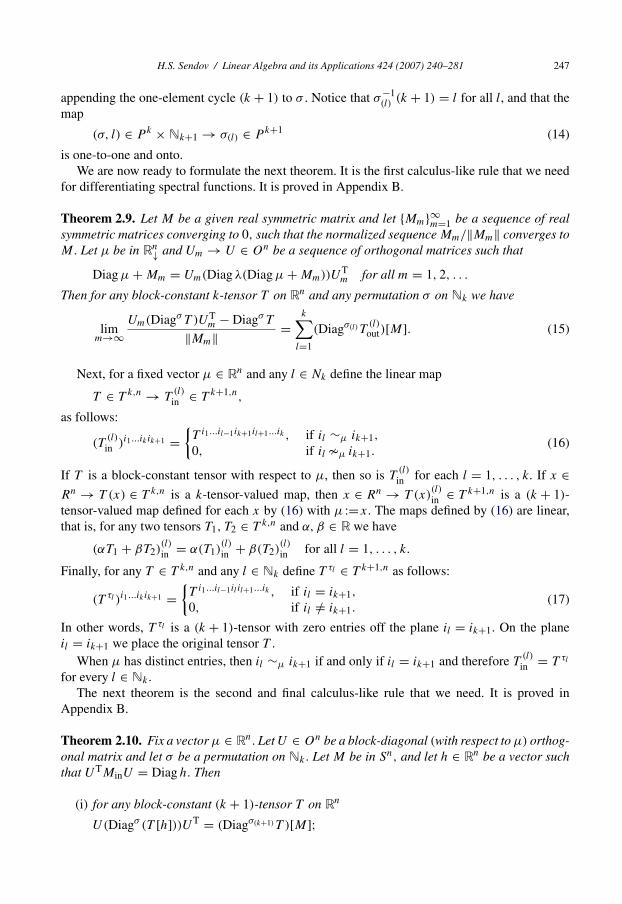
appending the one-element cycle (k + 1) to σ . Notice that σ−1(l) (k + 1) = l for all l, and that the
map
(σ, l) ∈ P k × Nk+1 → σ(l) ∈ P k+1 (14)
is one-to-one and onto.We are now ready to formulate the next theorem. It is the first calculus-like rule that we need
for differentiating spectral functions. It is proved in Appendix B.
Theorem 2.9. Let M be a given real symmetric matrix and let {Mm}∞m=1 be a sequence of realsymmetric matrices converging to 0, such that the normalized sequence Mm/‖Mm‖ converges toM. Let μ be in Rn↓ and Um → U ∈ On be a sequence of orthogonal matrices such that
Diag μ + Mm = Um(Diag λ(Diag μ + Mm))UTm for all m = 1, 2, . . .
Then for any block-constant k-tensor T on Rn and any permutation σ on Nk we have
limm→∞
Um(Diagσ T )UTm − Diagσ T
‖Mm‖ =k∑
l=1
(Diagσ(l)T(l)
out)[M]. (15)
Next, for a fixed vector μ ∈ Rn and any l ∈ Nk define the linear map
T ∈ T k,n → T(l)in ∈ T k+1,n,
as follows:
(T(l)in )i1...ik ik+1 =
{T i1...il−1ik+1il+1...ik , if il ∼μ ik+1,
0, if il �μ ik+1.(16)
If T is a block-constant tensor with respect to μ, then so is T(l)
in for each l = 1, . . . , k. If x ∈Rn → T (x) ∈ T k,n is a k-tensor-valued map, then x ∈ Rn → T (x)
(l)in ∈ T k+1,n is a (k + 1)-
tensor-valued map defined for each x by (16) with μ :=x. The maps defined by (16) are linear,that is, for any two tensors T1, T2 ∈ T k,n and α, β ∈ R we have
(αT1 + βT2)(l)in = α(T1)
(l)in + β(T2)
(l)in for all l = 1, . . . , k.
Finally, for any T ∈ T k,n and any l ∈ Nk define T τl ∈ T k+1,n as follows:
(T τl )i1...ik ik+1 ={T i1...il−1il il+1...ik , if il = ik+1,
0, if il /= ik+1.(17)
In other words, T τl is a (k + 1)-tensor with zero entries off the plane il = ik+1. On the planeil = ik+1 we place the original tensor T .
When μ has distinct entries, then il ∼μ ik+1 if and only if il = ik+1 and therefore T(l)
in = T τl
for every l ∈ Nk .The next theorem is the second and final calculus-like rule that we need. It is proved in
Appendix B.
Theorem 2.10. Fix a vector μ ∈ Rn. Let U ∈ On be a block-diagonal (with respect to μ) orthog-onal matrix and let σ be a permutation on Nk. Let M be in Sn, and let h ∈ Rn be a vector suchthat UTMinU = Diag h. Then
(i) for any block-constant (k + 1)-tensor T on Rn
U(Diagσ (T [h]))UT = (Diagσ(k+1)T )[M];

248 H.S. Sendov / Linear Algebra and its Applications 424 (2007) 240–281
(ii) for any block-constant k-tensor T on Rn
U(Diagσ (T τl [h]))UT = (Diagσ(1)T(l)in )[M] for all l = 1, . . . , k,
where the permutations σ(1), for l ∈ Nk, are defined by (13).
3. Several standing assumptions
Suppose f : Rn → R is a k-times differentiable symmetric function. For any integer s ∈ [1, k),in order to obtain the (s + 1)th derivative ∇s+1(f ◦ λ)(X) of the composition f ◦ λ, we differenti-ate ∇s(f ◦ λ)(X) and use the tensorial language presented in Section 2 to simplify the calculation.More precisely, for each σ ∈ P s we define a s-tensor-valued map Aσ : Rn → T s,n, dependingonly on the function f and its partial derivatives, such that
∇s(f ◦ λ)(X) = V
(∑σ∈P s
DiagσAσ (λ(X))
)V T, (18)
where X = V (Diag λ(X))V T.By [22, Section 5] it is enough to prove (18) only when X is an ordered diagonal matrix. That
is, X = Diag μ for some vector μ ∈ Rn↓.That (18) holds when s = 1 was shown in [13], see also Subsection 5.2.Let {Mm}∞m=1 be any sequence of real symmetric matrices converging to 0. In order to show
that
limm→∞
∇s(f ◦ λ)(X + Mm) − ∇s(f ◦ λ)(X) − ∇s+1(f ◦ λ)(X)[Mm]‖Mm‖ = 0
for s = 1, . . . , k − 1, we may assume without loss of generality that Mm/‖Mm‖ converges toa symmetric matrix M . Thus, we assume throughout that {Mm}∞m=1 is any sequence of realsymmetric matrices converging to 0 with Mm/‖Mm‖ converging to M ∈ Sn and show inductivelythat
limm→∞
∇s(f ◦ λ)(X + Mm) − ∇s(f ◦ λ)(X)
‖Mm‖= ∇s+1(f ◦ λ)(X)[M], for s = 1, . . . , k − 1. (19)
Finally, we denote by {Um}∞m=1 a sequence of orthogonal matrices in On, converging to U ∈ On
and such that
Diag μ + Mm = Um(Diag λ(Diag μ + Mm))UTm for all m = 1, 2, . . . (20)
The next lemma combines [14, Lemma 5.10] and [7, Theorem 3.12].
Lemma 3.1. For any μ ∈ Rn↓ and any sequence of real symmetric matrices Mm → 0 we have
λ(Diag μ + Mm)T = μT + (λ(XT1 MmX1)
T, . . . , λ(XTr MmXr)
T)T + o(‖Mm‖), (21)
where Xl :=[ei |i ∈ Il] for all l = 1, . . . , r .
We denote
hm := (λ(XT1 MmX1)
T, . . . , λ(XTr MmXr)
T)T. (22)
H.S. Sendov / Linear Algebra and its Applications 424 (2007) 240–281 249
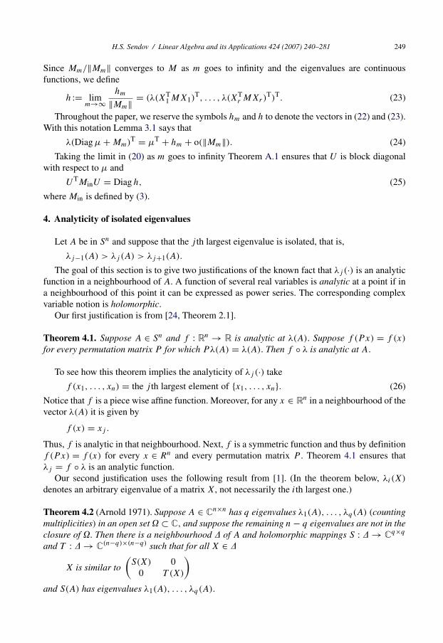
Since Mm/‖Mm‖ converges to M as m goes to infinity and the eigenvalues are continuousfunctions, we define
h := limm→∞
hm
‖Mm‖ = (λ(XT1 MX1)
T, . . . , λ(XTr MXr)
T)T. (23)
Throughout the paper, we reserve the symbols hm and h to denote the vectors in (22) and (23).With this notation Lemma 3.1 says that
λ(Diag μ + Mm)T = μT + hm + o(‖Mm‖). (24)
Taking the limit in (20) as m goes to infinity Theorem A.1 ensures that U is block diagonalwith respect to μ and
UTMinU = Diag h, (25)
where Min is defined by (3).
4. Analyticity of isolated eigenvalues
Let A be in Sn and suppose that the j th largest eigenvalue is isolated, that is,
λj−1(A) > λj (A) > λj+1(A).
The goal of this section is to give two justifications of the known fact that λj (·) is an analyticfunction in a neighbourhood of A. A function of several real variables is analytic at a point if ina neighbourhood of this point it can be expressed as power series. The corresponding complexvariable notion is holomorphic.
Our first justification is from [24, Theorem 2.1].
Theorem 4.1. Suppose A ∈ Sn and f : Rn → R is analytic at λ(A). Suppose f (Px) = f (x)
for every permutation matrix P for which Pλ(A) = λ(A). Then f ◦ λ is analytic at A.
To see how this theorem implies the analyticity of λj (·) take
f (x1, . . . , xn) = the j th largest element of {x1, . . . , xn}. (26)
Notice that f is a piece wise affine function. Moreover, for any x ∈ Rn in a neighbourhood of thevector λ(A) it is given by
f (x) = xj .
Thus, f is analytic in that neighbourhood. Next, f is a symmetric function and thus by definitionf (Px) = f (x) for every x ∈ Rn and every permutation matrix P . Theorem 4.1 ensures thatλj = f ◦ λ is an analytic function.
Our second justification uses the following result from [1]. (In the theorem below, λi(X)
denotes an arbitrary eigenvalue of a matrix X, not necessarily the ith largest one.)
Theorem 4.2 (Arnold 1971). Suppose A ∈ Cn×n has q eigenvalues λ1(A), . . . , λq(A) (countingmultiplicities) in an open set � ⊂ C, and suppose the remaining n − q eigenvalues are not in theclosure of �. Then there is a neighbourhood � of A and holomorphic mappings S : � → Cq×q
and T : � → C(n−q)×(n−q) such that for all X ∈ �
X is similar to
(S(X) 0
0 T (X)
)and S(A) has eigenvalues λ1(A), . . . , λq(A).
250 H.S. Sendov / Linear Algebra and its Applications 424 (2007) 240–281
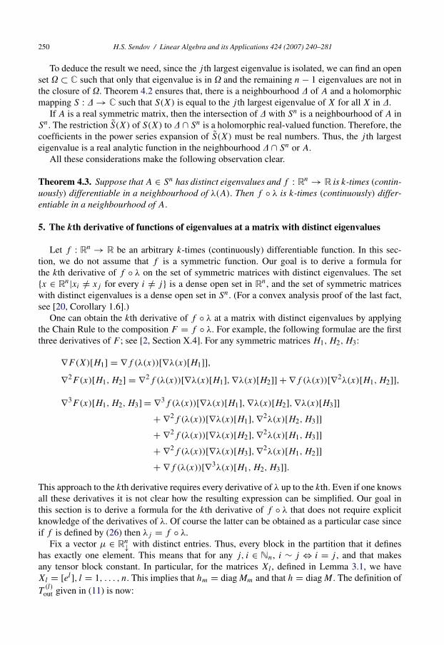
To deduce the result we need, since the j th largest eigenvalue is isolated, we can find an openset � ⊂ C such that only that eigenvalue is in � and the remaining n − 1 eigenvalues are not inthe closure of �. Theorem 4.2 ensures that, there is a neighbourhood � of A and a holomorphicmapping S : � → C such that S(X) is equal to the j th largest eigenvalue of X for all X in �.
If A is a real symmetric matrix, then the intersection of � with Sn is a neighbourhood of A inSn. The restriction S(X) of S(X) to � ∩ Sn is a holomorphic real-valued function. Therefore, thecoefficients in the power series expansion of S(X) must be real numbers. Thus, the j th largesteigenvalue is a real analytic function in the neighbourhood � ∩ Sn or A.
All these considerations make the following observation clear.
Theorem 4.3. Suppose that A ∈ Sn has distinct eigenvalues and f : Rn → R is k-times (contin-uously) differentiable in a neighbourhood of λ(A). Then f ◦ λ is k-times (continuously) differ-entiable in a neighbourhood of A.
5. The kth derivative of functions of eigenvalues at a matrix with distinct eigenvalues
Let f : Rn → R be an arbitrary k-times (continuously) differentiable function. In this sec-tion, we do not assume that f is a symmetric function. Our goal is to derive a formula forthe kth derivative of f ◦ λ on the set of symmetric matrices with distinct eigenvalues. The set{x ∈ Rn|xi /= xj for every i /= j} is a dense open set in Rn, and the set of symmetric matriceswith distinct eigenvalues is a dense open set in Sn. (For a convex analysis proof of the last fact,see [20, Corollary 1.6].)
One can obtain the kth derivative of f ◦ λ at a matrix with distinct eigenvalues by applyingthe Chain Rule to the composition F = f ◦ λ. For example, the following formulae are the firstthree derivatives of F ; see [2, Section X.4]. For any symmetric matrices H1, H2, H3:
∇F(X)[H1] = ∇f (λ(x))[∇λ(x)[H1]],∇2F(x)[H1, H2] = ∇2f (λ(x))[∇λ(x)[H1], ∇λ(x)[H2]] + ∇f (λ(x))[∇2λ(x)[H1, H2]],
∇3F(x)[H1, H2, H3] = ∇3f (λ(x))[∇λ(x)[H1], ∇λ(x)[H2], ∇λ(x)[H3]]+ ∇2f (λ(x))[∇λ(x)[H1], ∇2λ(x)[H2, H3]]+ ∇2f (λ(x))[∇λ(x)[H2], ∇2λ(x)[H1, H3]]+ ∇2f (λ(x))[∇λ(x)[H3], ∇2λ(x)[H1, H2]]+ ∇f (λ(x))[∇3λ(x)[H1, H2, H3]].
This approach to the kth derivative requires every derivative of λ up to the kth. Even if one knowsall these derivatives it is not clear how the resulting expression can be simplified. Our goal inthis section is to derive a formula for the kth derivative of f ◦ λ that does not require explicitknowledge of the derivatives of λ. Of course the latter can be obtained as a particular case sinceif f is defined by (26) then λj = f ◦ λ.
Fix a vector μ ∈ Rn↓ with distinct entries. Thus, every block in the partition that it defineshas exactly one element. This means that for any j, i ∈ Nn, i ∼ j ⇔ i = j , and that makesany tensor block constant. In particular, for the matrices Xl , defined in Lemma 3.1, we haveXl = [el], l = 1, . . . , n. This implies that hm = diag Mm and that h = diag M . The definition ofT
(l)out given in (11) is now:

H.S. Sendov / Linear Algebra and its Applications 424 (2007) 240–281 251
(T(l)out)
i1...ik ik+1 ={
0, if il = ik+1,T i1 ...il−1ik+1il+1 ...ik −T i1 ...il−1il il+1 ...ik
μik+1−μil, if il /= ik+1.
(27)
We derive (18) by induction on the order of the derivative.
5.1. Description of the kth derivative
Let f : Rn → R be k-times (continuously) differentiable function defined on the set
� :={x ∈ Rn|xi /= xj for every i /= j}.For every s ∈ Nk and every σ ∈ P s we define an s-tensor-valued map Aσ : � ⊂ Rn → T s,n
inductively, as follows. For s = 1 and σ = (1) we define
A(1)(x) :=∇f (x).
Assuming that the maps Aσ (x) have been defined for each σ ∈ P s with s ∈ [1, k) we define
Aσ(1)(x) := (Aσ (x))
(l)out for all l ∈ Ns , and
Aσ(s+1)(x) :=∇Aσ (x). (28)
We are now ready to formulate our first main theorem.
Theorem 5.1. Let X be a symmetric matrix with distinct eigenvalues. Let f be a function definedon a neighbourhood of λ(X). Then the spectral function F = f ◦ λ is k-times (continuously)differentiable at X if and only if f is k-times (continuously) differentiable at λ(X). Moreover,
∇kF (X) = V
⎛⎝∑σ∈P k
DiagσAσ (λ(X))
⎞⎠V T, (29)
where V is any orthogonal matrix such that X = V (Diag λ(X))V T.
The proof proceeds by induction and is presented in the next two subsections.
5.2. Proof of Theorem 5.1: the gradient
Using (24) we compute
limm→∞
(f ◦ λ)(Diag μ + Mm) − (f ◦ λ)(Diag μ)
‖Mm‖= lim
m→∞f (μ + hm + o(‖Mm‖)) − f (μ)
‖Mm‖= lim
m→∞f (μ) + ∇f (μ)[hm] + o(‖Mm‖) − f (μ)
‖Mm‖= ∇f (μ)[h]= 〈∇f (μ), diag M〉= (Diag ∇f (μ))[M].

252 H.S. Sendov / Linear Algebra and its Applications 424 (2007) 240–281
This shows that ∇(f ◦ λ)(Diag μ) = Diag(1)∇f (μ). One can see now that
∇(f ◦ λ)(X) = V (Diag(1)∇f (λ(X)))V T = V
⎛⎝∑σ∈P 1
DiagσAσ (λ(X))
⎞⎠V T, (30)
where X = V (Diag λ(X))V T and A(1)(x) = ∇f (x). If f is k-times (continuously) differentia-ble, then A(1)(x) = ∇f (x) is (k − 1)-times (continuously) differentiable.
If the eigenvalues of X are not distinct and f is a symmetric function, calculation of the gradientof f ◦ λ is almost identical and leads to the same final formula. Indeed, using (25) we get
∇f (μ)[h] = 〈∇f (μ), diag (UTMinU)〉 = (U(Diag ∇f (μ))UT)[M] = (Diag ∇f (μ))[M].In the last equality we used Lemma 2.1(i), U is block diagonal and orthogonal, and f is symmetric,so ∇f (μ) is block constant.
5.3. Proof of Theorem 5.1: the induction step
Suppose now that for some 1 � s < k
∇s(f ◦ λ)(X) = V
(∑σ∈P s
DiagσAσ (λ(X))
)V T,
where X = V (Diag λ(X))V T. Suppose also that for every σ ∈ P s , the s-tensor-valued map Aσ :Rn → T s,n is (k − s)-times (continuously) differentiable.
Using (24), we differentiate ∇s(f ◦ λ) at Diag μ:
∇s+1(f ◦ λ)(Diag μ)[M]= lim
m→∞∇s(f ◦ λ)(Diag μ + Mm) − ∇s(f ◦ λ)(Diag μ)
‖Mm‖
= limm→∞
Um
(∑σ∈P s DiagσAσ (λ(Diag μ + Mm))
)UT
m −∑σ∈P s DiagσAσ (μ)
‖Mm‖
= limm→∞
∑σ∈P s
Um(DiagσAσ (λ(Diag μ + Mm)))UTm − DiagσAσ (μ)
‖Mm‖
= limm→∞
∑σ∈P s
Um(DiagσAσ (μ + hm + o(‖Mm‖)))UTm − DiagσAσ (μ)
‖Mm‖
= limm→∞
∑σ∈P s
Um(Diagσ (Aσ (μ) + ∇Aσ (μ)[hm] + o(‖Mm‖)))UTm − DiagσAσ (μ)
‖Mm‖
= limm→∞
∑σ∈P s
Um(DiagσAσ (μ))UTm − DiagσAσ (μ)
‖Mm‖+∑σ∈P s
U(Diagσ (∇Aσ (μ)[h]))UT.
H.S. Sendov / Linear Algebra and its Applications 424 (2007) 240–281 253
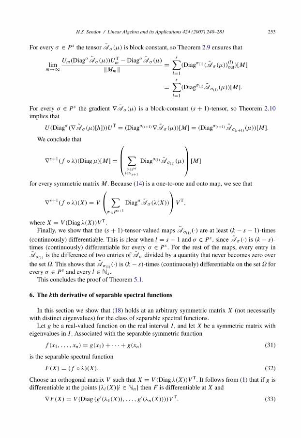
For every σ ∈ P s the tensor Aσ (μ) is block constant, so Theorem 2.9 ensures that
limm→∞
Um(DiagσAσ (μ))UTm − DiagσAσ (μ)
‖Mm‖ =s∑
l=1
(Diagσ(1) (Aσ (μ))(l)out)[M]
=s∑
l=1
(Diagσ(1)Aσ(1)(μ))[M].
For every σ ∈ P s the gradient ∇Aσ (μ) is a block-constant (s + 1)-tensor, so Theorem 2.10implies that
U(Diagσ (∇Aσ (μ)[h]))UT = (Diagσ(s+1)∇Aσ (μ))[M] = (Diagσ(s+1)Aσ(s+1)(μ))[M].
We conclude that
∇s+1(f ◦ λ)(Diag μ)[M] =
⎛⎜⎜⎝ ∑σ∈Ps
l∈Ns+1
Diagσ(1)Aσ(1)(μ)
⎞⎟⎟⎠ [M]
for every symmetric matrix M . Because (14) is a one-to-one and onto map, we see that
∇s+1(f ◦ λ)(X) = V
⎛⎝ ∑σ∈P s+1
DiagσAσ (λ(X))
⎞⎠V T,
where X = V (Diag λ(X))V T.Finally, we show that the (s + 1)-tensor-valued maps Aσ(1)
(·) are at least (k − s − 1)-times
(continuously) differentiable. This is clear when l = s + 1 and σ ∈ P s , since Aσ (·) is (k − s)-times (continuously) differentiable for every σ ∈ P s . For the rest of the maps, every entry inAσ(1)
is the difference of two entries of Aσ divided by a quantity that never becomes zero over
the set �. This shows that Aσ(1)(·) is (k − s)-times (continuously) differentiable on the set � for
every σ ∈ P s and every l ∈ Ns .This concludes the proof of Theorem 5.1.
6. The kth derivative of separable spectral functions
In this section we show that (18) holds at an arbitrary symmetric matrix X (not necessarilywith distinct eigenvalues) for the class of separable spectral functions.
Let g be a real-valued function on the real interval I , and let X be a symmetric matrix witheigenvalues in I . Associated with the separable symmetric function
f (x1, . . . , xn) = g(x1) + · · · + g(xn) (31)
is the separable spectral function
F(X) = (f ◦ λ)(X). (32)
Choose an orthogonal matrix V such that X = V (Diag λ(X))V T. It follows from (1) that if g isdifferentiable at the points {λi(X)|i ∈ Nn} then F is differentiable at X and
∇F(X) = V (Diag (g′(λ1(X)), . . . , g′(λn(X))))V T. (33)
254 H.S. Sendov / Linear Algebra and its Applications 424 (2007) 240–281
Separable spectral functions and their derivatives are of great importance for modern opti-mization; see [3,12,23]. For the role of general spectral functions see the two survey papers[15,16].
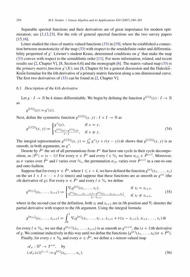
Löner studied the class of matrix-valued functions (33) in [19], where he established a connec-tion between monotonicity of the map (33) with respect to the semidefinite order and differentia-bility propertied of g′. Löwner’s student Kraus, determined conditions on g′ that make the map(33) convex with respect to the semidifinite order [11]. For more information, related, and recentresults see [2, Chapter V], [8, Section 6.6] and the monograph [6]. The matrix-valued map (33) isthe primary matrix function g′(X); see [8, Chapter 6] for a general discussion and the Daleckii–Krein formulae for the kth derivative of a primary matrix function along a one dimensional curve.The first two derivatives of (33) can be found in [2, Chapter V].
6.1. Description of the kth derivative
Let g : I → R be k-times differentiable. We begin by defining the function g[(1)](x) : I → R
as
g[(1)](x) :=g′(x).
Next, define the symmetric function g[(12)](x, y) : I × I → R as
g[(12)](x, y) :={
g′′(x), if x = y,
g[(1)](x)−g[(1)](y)x−y
, if x /= y.(34)
The integral representation g[(12)](x, y) = ∫ 10 g′′(y + t (x − y)) dt shows that g[(12)](x, y) is as
smooth, in both arguments, as g′′.Denote by P s the set of all permutations from P s that have one cycle in their cycle decompo-
sition, so |P s | = (s − 1)! For every σ ∈ P s and every l ∈ Ns we have σ(1) ∈ P s+1. Moreover,as σ varies over P s and l varies over Ns , the permutation σ(1) varies over P s+1 in a one-to-oneand onto fashion.
Suppose that for every σ ∈ P s , where 1 � s < k, we have defined the function g[σ ](x1, . . . , xs)
on the set I × I × · · · × I (s times) and suppose that these functions are as smooth as g(s) (thesth derivative of g). For every σ ∈ P s and every l ∈ Ns we define
g[σ(1)](x1, . . . , xs+1) :={∇lg
[σ ](x1, . . . , xs), if xl = xs+1,
g[σ ](x1,...,xl ,...,xs )−g[σ ](x1,...,xs+1,...,xs )
xl−xs+1, if xl /= xs+1,
(35)
where in the second case of the definition, both xl and xs+1 are in lth position and ∇l denotes thepartial derivative with respect to the lth argument. Using the integral formula
g[σ(1)](x1, . . . , xs+1) =∫ 1
0∇lg
[σ ](x1, . . . , xl−1, xs+1 + t (xl − xs+1), xl+1, . . . , xs) dt
for every l ∈ Ns , we see that g[σ(1)](x1, . . . , xs+1) is as smooth as g(s+1), the (s + 1)th derivativeof g. We continue inductively in this way until we define the functions {g[σ ](x1, . . . , xk)|σ ∈ P k}.
Finally, for every s ∈ Nk and every σ ∈ P s , we define a s-tensor-valued map
Aσ : Rn → T s,n, by
(Aσ (x))i1...is :=g[σ ](xi1 , . . . , xis ). (36)

H.S. Sendov / Linear Algebra and its Applications 424 (2007) 240–281 255
If (i1, . . . , is) ∼x (j1, . . . , js), then (Aσ (x))i1...is = (Aσ (x))j1...js , which shows that (36) definesa block-constant map; moreover, it is as smooth as g(s) for every s ∈ Nk .
We are now ready to formulate our second main theorem.
Theorem 6.1. Let g be a k-times differentiable real-valued function defined on a real inter-val I. Let X ∈ Sn have eigenvalues in I, and let V be an orthogonal matrix such that X =V (Diag λ(X))V T. Then the separable spectral function F defined by (31) and (32) is k-timesdifferentiable at X, and its kth derivative is
∇kF (X) = V
⎛⎝∑σ∈P k
DiagσAσ (λ(X))
⎞⎠V T, (37)
where Aσ (x) ≡ 0 if σ /∈ P k.
The proof is given in the next subsection. We proceed by induction—consecutively differen-tiating F(X). In the base case k = 1, (37) reduces to the formula for the gradient (33).
6.2. Proof of Theorem 6.1: the induction step
Suppose that g : I → R is k-times differentiable and the formula for the sth derivative (1 �s < k) of F at the matrix X is given by
∇sF (X) = V
(∑σ∈P s
DiagσAσ (λ(X))
)V T = V
⎛⎝∑σ∈P s
DiagσAσ (λ(X))
⎞⎠V T.
For each σ ∈ P s , the s-tensor-valued map Aσ : R → T s,n is (k − s)-times differentiable. InSection 3 we have described the simplifying assumptions and notation that we use below. We nowdifferentiate:
∇(s+1)F (Diag μ)[M]= lim
m→∞∇sF (Diag μ + Mm) − ∇sF (Diag μ)
‖Mm‖= lim
m→∞Um
(∑σ∈P s DiagσAσ (λ(Diag μ + Mm))
)UT
m −∑σ∈P s DiagσAσ (μ)
‖Mm‖= lim
m→∞∑σ∈P s
Um(DiagσAσ (μ + hm + o(‖Mm‖)))UTm − DiagσAσ (μ)
‖Mm‖
= limm→∞
∑σ∈P s
Um(Diagσ (Aσ (μ) + ∇Aσ (μ)[hm] + o(‖Mm‖)))UTm − DiagσAσ (μ)
‖Mm‖
= limm→∞
∑σ∈P s
Um(DiagσAσ (μ))UTm − DiagσAσ (μ)
‖Mm‖
+ U
⎛⎝∑σ∈P s
Diagσ (∇Aσ (μ)[h])⎞⎠UT.

256 H.S. Sendov / Linear Algebra and its Applications 424 (2007) 240–281
Using Theorem 2.9, we wrap up the first summand in the last expression:
limm→∞
∑σ∈P s
Um(DiagσAσ (μ))UTm − DiagσAσ (μ)
‖Mm‖=∑σ∈P s
l∈Ns
(Diagσ(1) (Aσ (μ))(l)out)[M]. (38)
Next, we focus our attention on the gradient ∇Aσ (μ). Using the definition, (36), and the chainrule, we get
∇[(Aσ (μ))i1...is ] =s∑
l=1
∇lg[σ ](μi1 , . . . , μis )e
il =s∑
l=1
g[σ(1)](μi1 , . . . , μis , μil )eil , (39)
where we used (35) to obtain the second equality. For convenience, for every σ ∈ P s and everyl ∈ Ns we define the map T l
σ : Rn → T s,n by
(T lσ (μ))i1...is :=g[σ(1)](μi1 , . . . , μis , μil ). (40)
Each of these maps is block constant.
Lemma 6.2. The gradient of Aσ (μ) can be decomposed as
∇Aσ (μ) =s∑
l=1
(T lσ (μ))τl , (41)
where the “lifting” (T lσ (μ))τl is defined by (17).
Proof. Fix a multi index (i1, . . . , is). By definition of the gradient ∇Aσ (μ) we have
∇[(Aσ (μ))i1...is ] = ((∇Aσ (μ))i1...is ,1, (∇Aσ (μ))i1...is ,2, . . . , (∇Aσ (μ))i1...is ,n)T.
We compute the pth entry in the last vector. Using (39), we get
(∇Aσ (μ))i1...is ,p =s∑
l=1il=p
g[σ(1)](μi1 , . . . , μis , μil ).
Using (17) and (40), we evaluate the right-hand side of (41):(s∑
l=1
(T lσ (μ))τl
)i1...is ,p
=s∑
l=1
((T lσ (μ))τl )i1...is ,p
=s∑
l=1
(T lσ (μ))i1...is δilp
=s∑
l=1il=p
(T lσ (μ))i1...is
=s∑
l=1il=p
g[σ(1)](μi1 , . . . , μis , μil ).
The lemma follows. �
H.S. Sendov / Linear Algebra and its Applications 424 (2007) 240–281 257
Using (41) we return to the second term in the differentiation of ∇sF (X):
U
⎛⎝∑σ∈P s
Diagσ (∇Aσ (μ)[h])⎞⎠UT = U
⎛⎝∑σ∈P s
Diagσ
((s∑
l=1
(T lσ (μ))τl
)[h])⎞⎠UT
= U
⎛⎝∑σ∈P s
s∑l=1
Diagσ ((T lσ (μ))τl [h])
⎞⎠UT
=∑σ∈P s
l∈Ns
U(Diagσ ((T lσ (μ))τl [h]))UT
=∑σ∈P s
l∈Ns
(Diagσ(1) (T lσ (μ))
(l)in )[M]; (42)
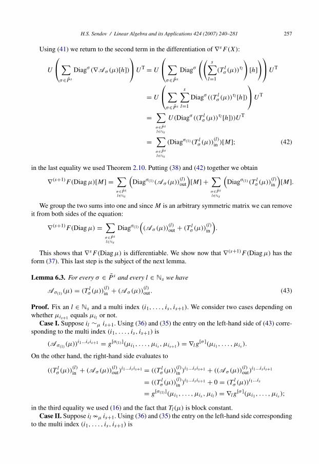
in the last equality we used Theorem 2.10. Putting (38) and (42) together we obtain
∇(s+1)F (Diag μ)[M] =∑σ∈P s
l∈Ns
(Diagσ(1) (Aσ (μ))
(l)out
)[M] +
∑σ∈P s
l∈Ns
(Diagσ(1) (T l
σ (μ))(l)in
)[M].
We group the two sums into one and since M is an arbitrary symmetric matrix we can removeit from both sides of the equation:
∇(s+1)F (Diag μ) =∑σ∈P s
l∈Ns
Diagσ(1)
((Aσ (μ))
(l)out + (T l
σ (μ))(l)in
).
This shows that ∇sF (Diag μ) is differentiable. We show now that ∇(s+1)F (Diag μ) has theform (37). This last step is the subject of the next lemma.
Lemma 6.3. For every σ ∈ P s and every l ∈ Ns we have
Aσ(1)(μ) = (T l
σ (μ))(l)in + (Aσ (μ))
(l)out. (43)
Proof. Fix an l ∈ Ns and a multi index (i1, . . . , is , is+1). We consider two cases depending onwhether μis+1 equals μil or not.
Case I. Suppose il ∼μ is+1. Using (36) and (35) the entry on the left-hand side of (43) corre-sponding to the multi index (i1, . . . , is , is+1) is
(Aσ(1)(μ))i1...is is+1 = g[σ(1)](μi1 , . . . , μis , μis+1) = ∇lg
[σ ](μi1 , . . . , μis ).
On the other hand, the right-hand side evaluates to
((T lσ (μ))
(l)in + (Aσ (μ))
(l)out)
i1...is is+1 = ((T lσ (μ))
(l)in )i1...is is+1 + ((Aσ (μ))
(l)out)
i1...is is+1
= ((T lσ (μ))
(l)in )i1...is is+1 + 0 = (T l
σ (μ))i1...is
= g[σ(1)](μi1 , . . . , μis , μil ) = ∇lg[σ ](μi1 , . . . , μis );
in the third equality we used (16) and the fact that Tl(μ) is block constant.Case II. Suppose il �μ is+1. Using (36) and (35) the entry on the left-hand side corresponding
to the multi index (i1, . . . , is , is+1) is

258 H.S. Sendov / Linear Algebra and its Applications 424 (2007) 240–281
(Aσ(1)(μ))i1...is is+1 = g[σ(1)](μi1 , . . . , μis , μis+1)
= g[σ ](μi1 , . . . , μil , . . . , μis ) − g[σ ](μi1 , . . . , μis+1 , . . . , μis )
μil − μis+1
,
where both μil and μis+1 are in the lth position. On the other hand, the right-hand side evaluatesto
((T lσ (μ))
(l)in + (Aσ (μ))
(l)out)
i1...is is+1
= ((T lσ (μ))
(l)in )i1...is is+1 + ((Aσ (μ))
(l)out)
i1...is is+1
= 0 + ((Aσ (μ))(l)out)
i1...is is+1
= (Aσ (μ))i1...il−1is+1il+1...is − (Aσ (μ))i1...il−1il il+1...is
μis+1 − μil
= g[σ ](μi1 , . . . , μis+1 , . . . , μis ) − g[σ ](μi1 , . . . , μil , . . . , μis )
μis+1 − μil
.
In both cases, the two sides are equal. �
This concludes the inductive step and the proof of Theorem 6.1.The two separate developments in Section 5 and Section 6 must be reconciled in their common
case. This is done by the following theorem proved in Appendix C.
Theorem 6.4. Suppose that X ∈ Sn has distinct eigenvalues, and the spectral function F isseparable and k-times differentiable at X. Then the two formulae for the kth derivative of F atX, namely, the one given in Theorem 5.1 where the operators Aσ are defined by the inductiveequations (28), and the one in Theorem 6.1 where the operators Aσ are defined by equations(36), are the same. More precisely we have∑
σ∈P s
DiagσAσ (x) =∑σ∈P s
DiagσAσ (x) for every s = 1, 2, . . . , k,
where x = λ(X).
It is worth presenting a particular case of Theorem 6.1. More specializations of Theorem 6.1,when g is Ck , are given in Subsubsection 6.3.1.
Corollary 6.5. Let g be twice differentiable in I, let X ∈ Sn have all eigenvalues in I, andsuppose that X = V (Diag λ(X))V T for some orthogonal matrix V . Then
∇2F(X) = V (Diag(12)A(12)(λ(X)))V T, (44)
where A(12)(·) is defined by
Aij
(12)(x) ={
g′′(xi), if xi = xj ,g′(xi )−g′(xj )
xi−xj, if xi /= xj .
Using approximation techniques, it was shown in [2, Theorem V.3.3] that for any two symmetricmatrices H1 and H2
H.S. Sendov / Linear Algebra and its Applications 424 (2007) 240–281 259
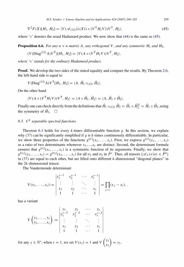
∇2F(X)[H1, H2] = 〈V (A(12)(λ(X)) ◦ (V TH1V ))V T, H2〉, (45)
where ‘◦’ denotes the usual Hadamard product. We now show that (44) is the same as (45).
Proposition 6.6. For any n × n matrix A, any orthogonal V, and any symmetric H1 and H2,
(V (Diag(12)A)V T)[H1, H2] = 〈V (A ◦ (V TH1V ))V T, H2〉,where ‘◦’ stands for the ordinary Hadamard product.
Proof. We develop the two sides of the stated equality and compare the results. By Theorem 2.6,the left-hand side is equal to
V (Diag(12)A)V T[H1, H2] = 〈A, H1 ◦(12) H2〉.On the other hand
〈V (A ◦ (V TH1V ))V T, H2〉 = 〈A ◦ H1, H2〉 = 〈A, H1 ◦ H2〉.Finally one can check directly from the definitions that H1 ◦(12) H2 = H1 ◦ HT
2 = H1 ◦ H2, usingthe symmetry of H2. �
6.3. Ck separable spectral functions
Theorem 6.1 holds for every k-times differentiable function g. In this section, we explainwhy (37) can be significantly simplified if g is k-times continuously differentiable. In particular,we show three properties of the functions g[σ ](x1, . . . , xs). First, we express g[σ ](x1, . . . , xs)
as a ratio of two determinants whenever x1,…,xs are distinct. Second, the determinant formulaensures that g[σ ](x1, . . . , xs) is a symmetric function of its arguments. Finally, we show thatg[σ1](x1, . . . , xs) = g[σ2](x1, . . . , xs) for all σ1 and σ2 in P s . Thus, all tensors {Aσ (x)|σ ∈ P k}in (37) are equal to each other, but are lifted onto different k-dimensional “diagonal planes” inthe 2k-dimensional tensor.
The Vandermonde determinant
V (x1, . . . , xs) :=
∣∣∣∣∣∣∣∣∣xs−1
1 xs−12 · · · xs−1
s...
.... . .
...
x1 x2 · · · xs
1 1 · · · 1
∣∣∣∣∣∣∣∣∣ =∏j<i
(xj − xi),
has a variant
V
(y1, . . . , ys
x1, . . . , xs
):=
∣∣∣∣∣∣∣∣∣∣∣
y1 y2 · · · ys
xs−21 xs−2
2 · · · xs−2s
......
. . ....
x1 x2 · · · xs
1 1 · · · 1
∣∣∣∣∣∣∣∣∣∣∣for any y ∈ Rs ; when s = 1, we set V (x1) = 1 and V
(y1x1
)= y1.
260 H.S. Sendov / Linear Algebra and its Applications 424 (2007) 240–281
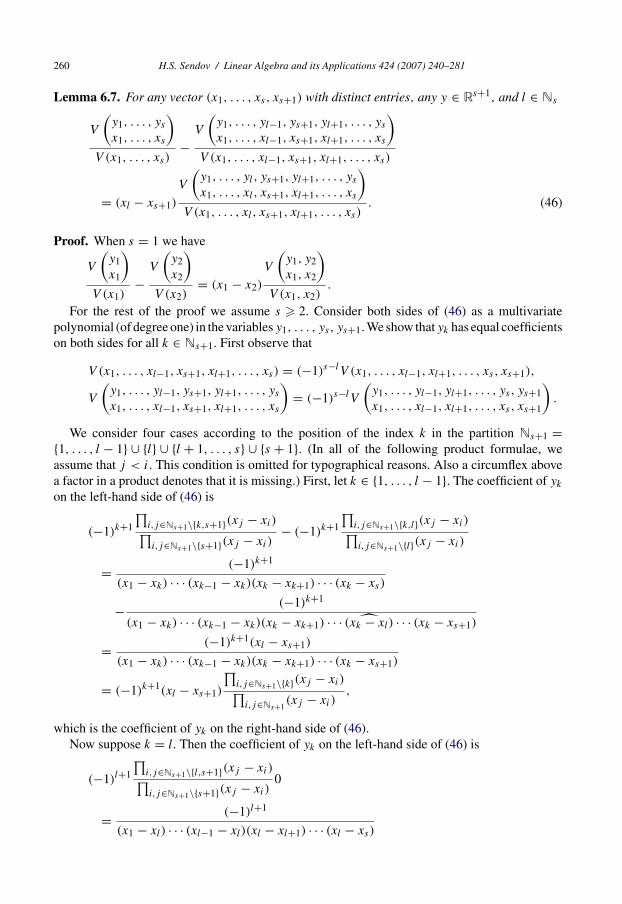
Lemma 6.7. For any vector (x1, . . . , xs, xs+1) with distinct entries, any y ∈ Rs+1, and l ∈ Ns
V
(y1, . . . , ys
x1, . . . , xs
)V (x1, . . . , xs)
−V
(y1, . . . , yl−1, ys+1, yl+1, . . . , ys
x1, . . . , xl−1, xs+1, xl+1, . . . , xs
)V (x1, . . . , xl−1, xs+1, xl+1, . . . , xs)
= (xl − xs+1)
V
(y1, . . . , yl, ys+1, yl+1, . . . , ys
x1, . . . , xl, xs+1, xl+1, . . . , xs
)V (x1, . . . , xl, xs+1, xl+1, . . . , xs)
. (46)
Proof. When s = 1 we have
V
(y1x1
)V (x1)
−V
(y2x2
)V (x2)
= (x1 − x2)
V
(y1, y2x1, x2
)V (x1, x2)
.
For the rest of the proof we assume s � 2. Consider both sides of (46) as a multivariatepolynomial (of degree one) in the variablesy1, . . . , ys, ys+1. We show thatyk has equal coefficientson both sides for all k ∈ Ns+1. First observe that
V (x1, . . . , xl−1, xs+1, xl+1, . . . , xs) = (−1)s−lV (x1, . . . , xl−1, xl+1, . . . , xs, xs+1),
V
(y1, . . . , yl−1, ys+1, yl+1, . . . , ys
x1, . . . , xl−1, xs+1, xl+1, . . . , xs
)= (−1)s−lV
(y1, . . . , yl−1, yl+1, . . . , ys, ys+1x1, . . . , xl−1, xl+1, . . . , xs, xs+1
).
We consider four cases according to the position of the index k in the partition Ns+1 ={1, . . . , l − 1} ∪ {l} ∪ {l + 1, . . . , s} ∪ {s + 1}. (In all of the following product formulae, weassume that j < i. This condition is omitted for typographical reasons. Also a circumflex abovea factor in a product denotes that it is missing.) First, let k ∈ {1, . . . , l − 1}. The coefficient of yk
on the left-hand side of (46) is
(−1)k+1
∏i,j∈Ns+1\{k,s+1}(xj − xi)∏i,j∈Ns+1\{s+1}(xj − xi)
− (−1)k+1
∏i,j∈Ns+1\{k,l}(xj − xi)∏i,j∈Ns+1\{l}(xj − xi)
= (−1)k+1
(x1 − xk) · · · (xk−1 − xk)(xk − xk+1) · · · (xk − xs)
− (−1)k+1
(x1 − xk) · · · (xk−1 − xk)(xk − xk+1) · · · (xk − xl) · · · (xk − xs+1)
= (−1)k+1(xl − xs+1)
(x1 − xk) · · · (xk−1 − xk)(xk − xk+1) · · · (xk − xs+1)
= (−1)k+1(xl − xs+1)
∏i,j∈Ns+1\{k}(xj − xi)∏
i,j∈Ns+1(xj − xi)
,
which is the coefficient of yk on the right-hand side of (46).Now suppose k = l. Then the coefficient of yk on the left-hand side of (46) is
(−1)l+1
∏i,j∈Ns+1\{l,s+1}(xj − xi)∏i,j∈Ns+1\{s+1}(xj − xi)
0
= (−1)l+1
(x1 − xl) · · · (xl−1 − xl)(xl − xl+1) · · · (xl − xs)

H.S. Sendov / Linear Algebra and its Applications 424 (2007) 240–281 261
= (−1)l+1(xl − xs+1)
(x1 − xl) · · · (xl−1 − xl)(xl − xl+1) · · · (xl − xs+1)
= (−1)l+1(xl − xs+1)
∏i,j∈Ns+1\{l}(xj − xi)∏
i,j∈Ns+1(xj − xi)
,
which is the corresponding coefficient on the right-hand side of (46).When k ∈ {l + 1, . . . , s}, the coefficient of yk on the left-hand side of (46) is
(−1)k+1
∏i,j∈Ns+1\{k,s+1}(xj − xi)∏i,j∈Ns+1\{s+1}(xj − xi)
− (−1)k
∏i,j∈Ns+1\{k,l}(xj − xi)∏i,j∈Ns+1\{l}(xj − xi)
= (−1)k+1
(x1 − xk) · · · (xk−1 − xk)(xk − xk+1) · · · (xk − xs)
− (−1)k
(x1 − xk) · · · (xl − xk) · · · (xk−1 − xk)(xk − xk+1) · · · (xk − xs+1)
= (−1)k+1(xl − xs+1)
(x1 − xk) · · · (xk−1 − xk)(xk − xk+1) · · · (xk − xs+1)
= (−1)k+1(xl − xs+1)
∏i,j∈Ns+1\{k}(xj − xi)∏
i,j∈Ns+1(xj − xi)
,
which is the coefficient of yk on the right-hand side.Finally, when k = s + 1 the coefficient of ys+1 on the left-hand side of (46) is
0 − (−1)l+1(−1)s−l
∏i,j∈Ns+1\{l,s+1}(xj − xi)∏
i,j∈Ns+1\{l}(xj − xi)
= (−1)s+2
(x1 − xs+1) · · · (xl − xs+1) · · · (xs − xs+1)
= (−1)s+2(xl − xs+1)
(x1 − xs+1) · · · (xs − xs+1)
= (−1)s+2(xl − xs+1)
∏i,j∈Ns+1\{s+1}(xj − xi)∏
i,j∈Ns+1(xj − xi)
,
which is again the coefficient of ys+1 on the right-hand side. �
Theorem 6.8. Suppose g ∈ Ck(I). Then for every permutation σ ∈ P s , where 1 � s � k, andevery vector (x1, . . . , xs) with distinct entries
g[σ ](x1, . . . , xs) =V
(g′(x1), . . . , g
′(xs)
x1, . . . , xs
)V (x1, . . . , xs)
. (47)
In particular, g[σ ](x1, . . . , xs) is a symmetric function.
262 H.S. Sendov / Linear Algebra and its Applications 424 (2007) 240–281
Proof. The proof is by induction on s. When s = 1, the definitions ensure that
g[(1)](x1) = g′(x1) =V
(g′(x1)
x1
)V (x1)
.
Suppose (47) holds for s, where 1 � s < k. Let (x1, . . . , xs, xs+1) be a vector with distinctentries and let y = (g′(x1), . . . , g
′(xs), g′(xs+1)). Fix a permutation σ ∈ P s and an index l ∈ Ns .
Using (35) together with Lemma 6.7 and the induction hypothesis we get
g[σ(1)](x1, . . . , xs, xs+1)
= g[σ ](x1, . . . , xs) − g[σ ](x1, . . . , xl−1, xs+1, xl+1, . . . , xs)
xl − xs+1
= 1
(xl − xs+1)
⎛⎜⎜⎝V
(y1, . . . , ys
x1, . . . , xs
)V (x1, . . . , xs)
−V
(y1, . . . , yl−1, ys+1, yl+1, . . . , ys
x1, . . . , xl−1, xs+1, xl+1, . . . , xs
)V (x1, . . . , xl−1, xs+1, xl+1, . . . , xs)
⎞⎟⎟⎠
=V
(y1, . . . , yl, ys+1, yl+1, . . . , ys
x1, . . . , xl, xs+1, xl+1, . . . , xs
)V (x1, . . . , xl, xs+1, xl+1, . . . , xs)
=V
(y1, . . . , ys+1x1, . . . , xs+1
)V (x1, . . . , xs+1)
.
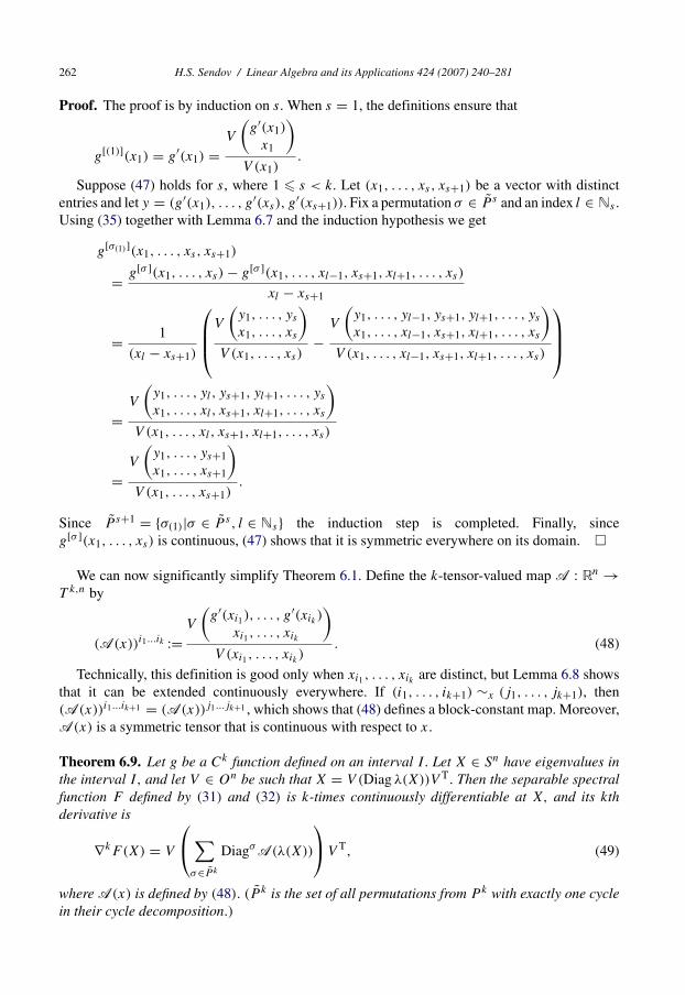
Since P s+1 = {σ(1)|σ ∈ P s , l ∈ Ns} the induction step is completed. Finally, sinceg[σ ](x1, . . . , xs) is continuous, (47) shows that it is symmetric everywhere on its domain. �
We can now significantly simplify Theorem 6.1. Define the k-tensor-valued map A : Rn →T k,n by
(A(x))i1...ik :=V
(g′(xi1), . . . , g
′(xik )
xi1 , . . . , xik
)V (xi1 , . . . , xik )
. (48)
Technically, this definition is good only when xi1 , . . . , xik are distinct, but Lemma 6.8 showsthat it can be extended continuously everywhere. If (i1, . . . , ik+1) ∼x (j1, . . . , jk+1), then(A(x))i1...ik+1 = (A(x))j1...jk+1 , which shows that (48) defines a block-constant map. Moreover,A(x) is a symmetric tensor that is continuous with respect to x.
Theorem 6.9. Let g be a Ck function defined on an interval I. Let X ∈ Sn have eigenvalues inthe interval I, and let V ∈ On be such that X = V (Diag λ(X))V T. Then the separable spectralfunction F defined by (31) and (32) is k-times continuously differentiable at X, and its kthderivative is
∇kF (X) = V
⎛⎝∑σ∈P k
DiagσA(λ(X))
⎞⎠V T, (49)
where A(x) is defined by (48). (P k is the set of all permutations from P k with exactly one cyclein their cycle decomposition.)

H.S. Sendov / Linear Algebra and its Applications 424 (2007) 240–281 263
For most practical applications of derivatives, it is important to know what the result is whenthey are viewed as multi-linear maps and applied to vectors from the underlying space.
The last part of this subsection is devoted to representations of the formula for the kth derivativeat X of a Ck separable spectral function, applied at k symmetric matrices.
6.3.1. Derivatives as multi linear operatorsThe next corollary specializes Theorem 6.9 to the case k = 3. It should be compared
with [2, (V.22)] and [8, §6.6]. One should keep in mind that we are differentiating separablespectral functions, whose gradients are the primary matrix functions considered in [2, ChapterV].
Corollary 6.10. For g ∈ C3(I ) and any H1, H2, H3 in Sn we have
∇3F(X)[H1, H2, H3] = 2n,n,n∑
p1,p2,p3=1
A(λ(X))p1p2p3Hp1p21 H
p2p32 H
p3p13 ,
where X = V (Diag λ(X))V T, and Hi = V THiV for i = 1, 2, 3.
Proof. Without loss of generality suppose that X = Diag μ for some μ ∈ Rn↓. Then
∇3F(Diag μ)[H1, H2, H3]
=⎛⎝∑
σ∈P 3
DiagσA(μ)
⎞⎠ [H1, H2, H3]
=∑
σ∈P 3
〈A(μ), H1 ◦σ H2 ◦σ H3〉
= 〈A(μ), H1 ◦(123) H2 ◦(123) H3〉 + 〈A(μ), H1 ◦(132) H2 ◦(132) H3〉
=n,n,n∑
q1,q2,q3=1
A(μ)q1q2q3Hq1q31 H
q2q12 H
q3q23 +
n,n,n∑p1,p2,p3=1
A(μ)p1p2p3Hp1p21 H
p2p32 H
p3p13 .
After re-parametrization of the first sum (q1 = p2, q2 = p3, q3 = p1), using the symmetry of thetensor A(μ) and the matrices H1, H2, H3, we continue
=n,n,n∑
p1,p2,p3=1
(A(μ)p2p3p1 + A(μ)p1p2p3)Hp1p21 H
p2p32 H
p3p13
= 2n,n,n∑
p1,p2,p3=1
A(μ)p1p2p3Hp1p21 H
p2p32 H
p3p13 ,
which is what we wanted to show. �
In the general case when H1,…,Hk are distinct symmetric matrices, we cannot simplify theformula for ∇kF (X)[H1, . . . , Hk] much more than the example in Corollary 6.10.
To show that we can do at least that much, let σ and θ be in P k , that is, permutations inP k with one cycle in their cycle decomposition. Suppose that σ = θ−1, that A is a symmetric

264 H.S. Sendov / Linear Algebra and its Applications 424 (2007) 240–281
k-tensor on Rn, and that H1,…,Hk are distinct symmetric matrices. Then, re-parameterizing thesum
n,...,n∑q1,...,qk=1
Aq1...qkHq1qσ−1(1)
1 · · · Hqkqσ−1(k)
k
according to the substitutions qi = pσ(i) for i = 1, 2, . . . , k we get the sum
n,...,n∑p1,...,pk=1
Apσ(1)...pσ(k)Hpσ(1)p11 · · · Hpσ(k)pk
k
=n,...,n∑
p1,...,pk=1
Ap1...pkHpσ(1)p11 · · · Hpσ(k)pk
k
=n,...,n∑
p1,...,pk=1
Ap1...pkHp1pθ−1(1)
1 · · · Hpkpθ−1(k)
k .
In the first equality above we used the fact that A is a symmetric tensor, while in the second weused that Hi is a symmetric matrix for i = 1, 2, . . . , k.
We summarize the preceding paragraph in the following theorem.
Theorem 6.11. Let P k0 be a subset of P k, k � 3, such that if σ ∈ P k
0 then σ−1 /∈ P k0 .
For g ∈ Ck(I) and any H1, . . . , Hk in Sn we have
∇kF (X)[H1, . . . , Hk] = 2∑
σ∈P k0
n,...,n∑p1,...,pk=1
A(λ(X))p1...pk Hp1pσ(1)
1 · · · H pkpσ(k)
k , (50)
where X = V (Diag λ(X))V T, and Hi = V THiV for i = 1, 2, . . . , k.
If, H1 = · · · = Hk then (50) can be simplified even more.
Theorem 6.12. For g ∈ Ck(I) and any H ∈ Sn
∇kF (X)[H, . . . , H ] = (k − 1)!n,...,n∑
p1,...,pk=1
A(λ(X))p1...pk H p1p2H p2p3 · · · H pkp1 , (51)
where X = V (Diag λ(X))V T, and H = V THV.
Proof. Let H be in Sn. Using (49), (10), and (5) we find
∇kF (X)[H, . . . , H ] = V
⎛⎝∑σ∈P k
DiagσA(λ(X))
⎞⎠V T[H, . . . , H ]
=∑
σ∈P k
〈A(λ(X)), H ◦σ H ◦σ · · · ◦σ H 〉
=∑
σ∈P k
n,...,n∑p1,...,pk=1
A(λ(X))p1...pk Hp1pσ−1(1) · · · H pkpσ−1(k) .
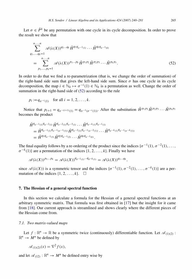
H.S. Sendov / Linear Algebra and its Applications 424 (2007) 240–281 265
Let σ ∈ P k be any permutation with one cycle in its cycle decomposition. In order to provethe result we show that
n,...,n∑q1,...,qk=1
A(λ(X))q1...qk Hq1qσ−1(1) · · · H qkqσ−1(k)
=n,...,n∑
p1,...,pk=1
A(λ(X))p1...pk H p1p2H p2p3 · · · H pkp1 . (52)
In order to do that we find a re-parametrization (that is, we change the order of summation) ofthe right-hand side sum that gives the left-hand side sum. Since σ has one cycle in its cycledecomposition, the map i ∈ Nk �→ σ−i (1) ∈ Nk is a permutation as well. Change the order ofsummation in the right-hand side of (52) according to the rule
pi :=qσ−i (1) for all i = 1, 2, . . . , k.
Notice that pi+1 = qσ−(i+1)(1) = qσ−1(σ−i (1)). After the substitution H p1p2H p2p3 · · · H pkp1
becomes the product
Hqσ−1(1)
qσ−2(1) H
qσ−2(1)
qσ−3(1) · · · H q
σ−k(1)qσ−1(1)
= Hqσ−1(1)
qσ−1(σ−1(1)) H
qσ−2(1)
qσ−1(σ−2(1)) · · · H q
σ−k(1)qσ−1(σ−k(1))
= Hq1qσ−1(1) H
q2qσ−1(2) · · · H qkqσ−1(k) .
The final equality follows by a re-ordering of the product since the indices {σ−1(1), σ−2(1), . . . ,
σ−k(1)} are a permutation of the indices {1, 2, . . . , k}. Finally we have
A(λ(X))p1...pk = A(λ(X))qθ−1(1)
...qθ−k(1) = A(λ(X))q1...qk ,
since A(λ(X)) is a symmetric tensor and the indices {σ−1(1), σ−2(1), . . . , σ−k(1)} are a per-mutation of the indices {1, 2, . . . , k}. �
7. The Hessian of a general spectral function
In this section we calculate a formula for the Hessian of a general spectral functions at anarbitrary symmetric matrix. That formula was first obtained in [17] but the insight for it camefrom [18]. Our current approach is streamlined and shows clearly where the different pieces ofthe Hessian come from.
7.1. Two matrix-valued maps
Let f : Rn → R be a symmetric twice (continuously) differentiable function. Let A(1)(2) :Rn → Mn be defined by
A(1)(2)(x) = ∇2f (x),
and let A(12) : Rn → Mn be defined entry wise by

266 H.S. Sendov / Linear Algebra and its Applications 424 (2007) 240–281
Ai1i2(12)(x) =
⎧⎪⎪⎨⎪⎪⎩0, if i1 = i2,
f ′′i1i1
(x) − f ′′i1i2
(x), if i1 ∼x i2 and i1 /= i2,
f ′i2
(x)−f ′i1
(x)
xi2 −xi1, if i1 �x i2.
Several of the properties of A(12)(x) are easily seen from the following integral representation.
Lemma 7.1. If f is a C2 function, then for every i1, i2 ∈ Nn we have
Ai1i2(12)(x) =
∫ 1
0f ′′
i1i1(. . . , xi1 + t (xi2 − xi1), . . . , xi2 + t (xi1 − xi2), . . .)
−f ′′i1i2
(. . . , xi1 + t (xi2 − xi1), . . . , xi2 + t (xi1 − xi2), . . .) dt,
where the first displayed argument is in position i1 and the second is in position i2. The missingarguments are the corresponding entries of x, unchanged.
Proof. The first case, when i1 = i2 is immediate. In the second, il ∼x i2 implies that xi1 = xi2
and the integrand does not depend on t . In the third case, i1 �x i2, the Fundamental Theorem ofCalculus, tell us that
1
xi2 − xi1
∫ 1
0
��t
f ′i1(. . . , xi1 + t (xi2 − xi1), . . . , xi2 + t (xi1 − xi2), . . .) dt
= f ′i1(. . . , xi2 , . . . , xi1 , . . .) − f ′
i1(. . . , xi1 , . . . , xi2 , . . .)
xi2 − xi1
= f ′i2(. . . , xi1 , . . . , xi2 , . . .) − f ′
i1(. . . , xi1 , . . . , xi2 , . . .)
xi2 − xi1
= Ai1i2(12)(x).
In the second equality we used that x �→ ∇f (x) is a point-symmetric map. �
Lemma 7.2. If f (x) is twice (continuously) differentiable, then both maps x → A(1)(2)(x) andx → A(12)(x) are point symmetric.
Proof. Lemma 2.5 shows that x �→ A(1)(2)(x) is point symmetric, so if i1 ∼x j1, then f ′′i1i1
(x) =f ′′
j1j1(μ). Also, if i1 ∼x j1 and i2 ∼x j2 with i1 /= i2 and j1 /= j2, then f ′′
i1i2(x) = f ′′
j1j2(x). Point
symmetry of x �→ ∇f (x) implies that if i1 ∼x j1, then f ′i1(x) = f ′
j1(x). �
Lemma 7.1 ensures that if f (x) is twice continuously differentiable then A(1)(2)(x) andA(12)(x) are symmetric matrices and are continuous in x.
7.2. f ◦ λ is twice (continuously) differentiable if and only if f is
We now show that f ◦ λ is twice (continuously) differentiable at X if and only if f is same atλ(X). The ‘only if’ direction can be seen by restricting f ◦ λ to the subspace of diagonal matrices.To show the ‘if’ direction, without loss of generality assume that X = Diag μ, for some μ ∈ Rn↓,that Mm/‖Mm‖ converges to M as m goes to infinity, and that (20) holds. Using (30) togetherwith (24) we compute:

H.S. Sendov / Linear Algebra and its Applications 424 (2007) 240–281 267
∇2(f ◦ λ)(Diag μ)[M]= lim
m→∞∇(f ◦ λ)(Diag μ + Mm) − ∇(f ◦ λ)(Diag μ)
‖Mm‖= lim
m→∞Um(Diag(1)∇f (λ(Diag μ + Mm)))UT
m − Diag(1)∇f (μ)
‖Mm‖= lim
m→∞Um(Diag(1)∇f (μ + hm + o(‖Mm‖)))UT
m − Diag(1)∇f (μ)
‖Mm‖= lim
m→∞Um(Diag(1)(∇f (μ) + ∇2f (μ)[hm] + o(‖Mm‖)))UT
m − Diag(1)∇f (μ)
‖Mm‖= lim
m→∞Um(Diag(1)(∇f (μ)))UT
m − Diag(1)∇f (μ)
‖Mm‖ + U(Diag(1)(∇2f (μ)[h]))UT.
(53)
For brevity let T = ∇f (μ), letA(1)(2) = A(1)(2)(μ), and letA(12) = A(12)(μ). Using Corollary2.9
limm→∞
Um(Diag(1)T )UTm − Diag(1)T
‖Mm‖ = (Diag(12)T(1)out )[M]. (54)
By Lemma 2.1 part (ii), there is a vector b that is block constant with respect to μ, such thatA(1)(2) − Diag b is also block constant with respect to μ. Then by Corollary 2.10, applied withk = 1,
U(Diag(1)(∇2f (μ)[h]))UT
= U(Diag(1)((A(1)(2) − Diag b + Diag b)[h]))UT
= U(Diag(1)((A(1)(2) − Diag b)[h]))UT + U(Diag(1)((Diag b)[h]))UT
= (Diag(1)(2)(A(1)(2) − Diag b))[M] + (Diag(12)b(1)in )[M]. (55)
This shows that f ◦ λ is twice differentiable.To prove that f ◦ λ is twice continuously differentiable we reorganize the pieces. Direct ver-
ification shows that the sum A(1)(2) + A(12) is block-constant. Then b can be chosen in such away that, in addition, A(12) + Diag b is a block-constant matrix and
A(12) + Diag b = T(1)
out + b(1)in . (56)
Putting (53)–(56) together we obtain:
∇2(f ◦ λ)(Diag μ) = Diag(12)T(1)
out + Diag(1)(2)(A(1)(2) − Diag b) + Diag(12)b(1)in
= Diag(1)(2)(A(1)(2) − Diag b) + Diag(12)(A(12) + Diag b)
= Diag(1)(2)A(1)(2) + Diag(12)A(12).
In the third equality we used the fact that Diag(1)(2)(Diag b) = Diag(12)(Diag b), which canbe verified directly. The formula for the Hessian of f ◦ λ at an arbitrary X is
∇2(f ◦ λ)(X) = V (Diag(1)(2)A(1)(2)(λ(X)) + Diag(12)A(12)(λ(X)))V T, (57)
where X = V (Diag λ(X))V T.
268 H.S. Sendov / Linear Algebra and its Applications 424 (2007) 240–281
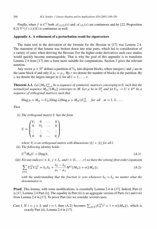
Finally, when f is C2 both A(1)(2)(x) and A(12)(x) are continuous and by [22, Proposition6.2] ∇2(f ◦ λ)(X) is continuous as well.
Appendix A. A refinement of a perturbation result for eigenvectors
The main tool in the derivation of the formula for the Hessian in [17] was Lemma 2.4.The statement of that lemma was broken down into nine parts, which led to consideration ofa variety of cases when deriving the Hessian. For the higher-order derivatives such case studieswould quickly become unmanageable. That is why the goal of this appendix is to transformLemma 2.4 from [17] into a form more suitable for computations. Section 3 gives the relevantnotation.
Any vector μ ∈ Rn defines a partition of Nn into disjoint blocks, where integers i and j are inthe same block if and only if μi = μj . By r we denote the number of blocks in the partition. Byιl we denote the largest integer in Il for all l = 1, . . . , r .
Theorem A.1. Let {Mm}∞m=1 be a sequence of symmetric matrices converging to 0, such that thenormalized sequence Mm/‖Mm‖ converges to M. Let μ be in Rn↓ and let Um → U ∈ On be asequence of orthogonal matrices such that
Diag μ + Mm = Um(Diag λ(Diag μ + Mm))UTm, for all m = 1, 2, . . . .
Then
(i) The orthogonal matrix U has the form
U =
⎛⎜⎜⎜⎝V1 0 · · · 00 V2 · · · 0...
.... . .
...
0 0 · · · Vr
⎞⎟⎟⎟⎠ ,
where Vl is an orthogonal matrix with dimensions |Il | × |Il | for all l.
(ii) The following identity holds:
UTMinU = Diag h, (A.1)
(iii) For any indices i ∈ Il, j ∈ Is, and t ∈ {1, . . . , r} we have the (strong) first-order expansion∑p∈It
Uipm U
jpm = δij δlt + δlt − δst
μi − μj
Mij‖Mm‖ + o(‖Mm‖), (A.2)
with the understanding that the fraction is zero whenever δlt = δst no matter what thedenominator is.
Proof. This lemma, with some modifications, is essentially Lemma 2.4 in [17]. Indeed, Part (i)is [17, Lemma 2.4 Part (i)]. The equality in Part (ii) is an aggregate version of Parts (iv) and (vii)from Lemma 2.4 in [17]. To prove Part (iii) we consider several cases.
Case 1. If i = j ∈ Il and t = l, then (A.2) becomes∑
p∈Il(U
ipm )2 = 1 + o(‖Mm‖), which is
exactly Part (ii), Lemma 2.4 in [17].

H.S. Sendov / Linear Algebra and its Applications 424 (2007) 240–281 269
Case 2. If i = j ∈ Il and t /= l, then (A.2) becomes∑
p∈It(U
ipm )2 = o(‖Mm‖), which is a con-
sequence of Part (iii), Lemma 2.4 in [17].Case 3. If i /= j ∈ Il and t = l, then (A.2) becomes
∑p∈Il
Uipm U
jpm = o(‖Mm‖), which is exactly
Part (vi), Lemma 2.4 in [17].Case 4. If i /= j ∈ Il and t /= l, then (A.2) becomes
∑p∈It
Uipm U
jpm = o(‖Mm‖), which is a con-
sequence of Part (v), Lemma 2.4 in [17].Case 5. If i ∈ Il , j ∈ Is , with l /= s /= t /= l, then (A.2) becomes
∑p∈It
Uipm U
jpm = o(‖Mm‖),
which is a consequence of Part (viii), Lemma 2.4 in [17].Case 6. If i ∈ Il , j ∈ Is , with l /= s and t = l, then (A.2) becomes∑
p∈It
Uipm U
jpm = 1
μi − μj
Mij‖Mm‖ + o(‖Mm‖),
which we prove in Case 7.Case 7. If i ∈ Il , j ∈ Is , with l /= s and t = s, then (A.2) becomes∑
p∈It
Uipm U
jpm = − 1
μi − μj
Mij‖Mm‖ + o(‖Mm‖).
We now show that the expressions in both Case 6 and Case 7 are valid. Part (ix) fromLemma 2.4 in [17] says that if i ∈ Il , j ∈ Is with l /= s, we have
limm→∞ g
(μιl
∑p∈Il
Uipm U
jpm
‖Mm‖ + μιs
∑p∈Is
Uipm U
jpm
‖Mm‖ g
)= Mij . (A.3)
Introduce the notation
βlm :=
∑p∈Il
Uipm U
jpm
‖Mm‖ for all l = 1, 2, . . . , r,
and notice thatr∑
l=1
βlm = 0 for all m,
because Um is orthogonal and the numerator of the last sum is the product of its ith andj th row. Next, by Case 5 we have
limm→∞
∑t /=l,s
βtm = 0,
so
limm→∞(βl
m + βsm) = 0.
For arbitrary reals a and b we compute
(aβlm + bβs
m) − a − b
μιl − μιs
(μιl βlm + μιs β
sm) = (βl
m + βsm)
bμιl − aμιs
μιl − μιs
→ 0,
as m → ∞. Using (A.3), this shows that
limm→∞(aβl
m + bβsm) = a − b
μιl − μιs
Mij .
When (a, b) = (1, 0) we obtain Case 6, and when (a, b) = (0, 1) we obtainCase 7. �

270 H.S. Sendov / Linear Algebra and its Applications 424 (2007) 240–281
Appendix B. Tensor analysis
The aim of this appendix is to prove Theorems 2.9 and 2.10.Recall that any vector μ ∈ Rn defines a partition of Nn into disjoint blocks, where integers i
and j are in the same block if and only if μi = μj . By r we denote the number of blocks in thepartition. By ιl we denote the largest integer in Il for all l = 1, . . . , r .
Theorem B.1. Let {Mm}∞m=1 be a sequence of symmetric matrices converging to 0, such thatthe normalized sequence Mm/‖Mm‖ converges to M. Let μ be in Rn↓ and Um → U ∈ On be asequence of orthogonal matrices such that
Diag μ + Mm = Um(Diag λ(Diag μ + Mm))UTm, for all m = 1, 2, . . . .
Then for every block-constant k-tensor T on Rn, any matrices H1, . . . , Hk , and any permutationσ on Nk we have
limm→∞
(Um(Diagσ T )UT
m − Diagσ T
‖Mm‖)
[H1, . . . , Hk]
=k∑
l=1
(Diagσ(1)T(l)out)[H1, . . . , Hk, Mout], (B.1)
where Mout is the symmetric matrix of off-diagonal blocks of M as defined by (4).
Proof. The idea of the proof is to evaluate separately the expressions on both sides of (B.1) andcompare the results. Both sides of (B.1) are linear in each argument Hs . That is why it is enoughto prove the result when Hs , for s = 1, . . . , k, is an arbitrary matrix, Hisjs , from the standard basison Mn. In that case
(Um(Diagσ T )UTm − Diagσ T )[Hi1j1 , . . . , Hikjk
]= (Um(Diagσ T )UT
m)i1 ...ikj1 ...jk − (Diagσ T )
i1 ...ikj1 ...jk . (B.2)
Using the definition of the conjugate action and the fact that T is block constant, we developthe first term on the right-hand side of the equality sign in (B.2):
(Um(Diagσ T )UTm)
i1 ...ikj1 ...jk =
n,...,n∑pη,qη=1η=1,...,k
(Diagσ T )p1 ...pkq1 ...qk
k∏ν=1
Uiνpνm U
jνqνm
=n,...,n∑pη=1
η=1,...,k
T p1...pk
k∏ν=1
Uiνpνm U
jνpσ−1(ν)
m
=n,...,n∑pη=1
η=1,...,k
T p1...pk
k∏ν=1
Uiνpνm U
jσ(ν)pνm
=r,...,r∑tη=1
η=1,...,k
T ιt1 ...ιtk
k∏ν=1
⎛⎝ ∑pν∈Itν
Uiνpνm U
jσ(ν)pνm
⎞⎠ .

H.S. Sendov / Linear Algebra and its Applications 424 (2007) 240–281 271
Putting everything together, we see that to evaluate the limit on the left-hand side of (B.1) wemust compute
limm→∞
∑r,...,rt1,...,tk=1T
ιt1 ...ιtk∏k
ν=1
(∑pν∈Itν
Uiνpνm U
jσ(ν)pνm
)− (Diagσ T )
i1 ...ikj1 ...jk
‖Mm‖ . (B.3)
Assume that il ∈ Ivland jσ(l) ∈ Isl for all l = 1, . . . , k. We investigate several possibilities.
Suppose first that among the pairs
(i1, jσ(1)), (i2, jσ(2)), . . . , (ik, jσ(k)) (B.4)
at least two have nonequal entries. Without loss of generality we may assume they are (i1, jσ(1))
and (i2, jσ(2)), that is, i1 /= jσ(1) and i2 /= jσ(2). Using (A.2), for any t1, t2 we observe that:
limm→∞
1
‖Mm‖
⎛⎝ ∑p1∈It1
Ui1p1m U
jσ(1)p1m
⎞⎠⎛⎝ ∑p2∈It2
Ui2p2m U
jσ(2)p2m
⎞⎠= lim
m→∞1
‖Mm‖
(δi1jσ(1)
δv1t1 + δv1t1 − δs1t1
μi1 − μjσ(1)
Mi1jσ(1)‖Mm‖ + o(‖Mm‖))
×(
δi2jσ(2)δv2t2 + δv2t2 − δs2t2
μi2 − μjσ(2)
Mi2jσ(2)‖Mm‖ + o(‖Mm‖))
= limm→∞
1
‖Mm‖
(δv1t1 − δs1t1
μi1 − μjσ(1)
Mi1jσ(1)‖Mm‖ + o(‖Mm‖))
×(
δv2t2 − δs2t2
μi2 − μjσ(2)
Mi2jσ(2)‖Mm‖ + o(‖Mm‖))
= 0.
Since in this case by definition (Diagσ T )i1 ...ikj1 ...jk = 0, we see that (B.3) is zero.
Suppose now that exactly one pair has unequal entries and let it be (il, jσ(l)). We consider twosubcases depending on whether or not il and jσ(l) are in the same block.
If both il and jσ(l) are in one block, that is, vl = sl , then using (A.2), for arbitrary t we obtain:
limm→∞
1
‖Mm‖
⎛⎝∑p∈It
Uilpm U
jσ(l)pm
⎞⎠= lim
m→∞1
‖Mm‖
(δiljσ(l)
δvl t + δvl t − δsl t
μil − μjσ(l)
Miljσ(l)‖Mm‖ + o(‖Mm‖))
= limm→∞
o(‖Mm‖)‖Mm‖
= 0.
In this subcase we again have (Diagσ T )i1 ...ikj1 ...jk = 0; thus (B.3) is equal to zero.

272 H.S. Sendov / Linear Algebra and its Applications 424 (2007) 240–281
If il and jσ(l) are in different blocks, vl /= sl , then (Diagσ T )i1 ...ikj1 ...jk = 0 and by (A.2) we obtain:
limm→∞
1
‖Mm‖
⎛⎝ r,...,r∑t1,...,tk=1
Tιt1 ...ιtk
k∏ν=1
⎛⎝ ∑pν∈Itν
Uiνpνm U
jσ(ν)pνm
⎞⎠⎞⎠= lim
m→∞
⎛⎝ r,...,r∑t1,...,tk=1
Tιt1 ...ιtk
‖Mm‖k∏
ν=1
(δiνjσ(ν)
δvν tν + δvν tν − δsν tν
μiν − μjσ(ν)
Miνjσ(ν)‖Mm‖ + o(‖Mm‖))⎞⎠ .
(B.5)
We show that the limit of at most two terms of the big sum in (B.5) may be non zero. Indeed, sum-mands corresponding to k-tuples (t1, . . . , tk) with tl /∈ {vl, sl} converge to zero, because δiljσ(l)
=0, δvl tl = δsl tl = 0, and therefore
δiljσ(l)δvl tl + δvl tl − δsl tl
μil − μjσ(l)
Miljσ(l)‖Mm‖ + o(‖Mm‖) = o(‖Mm‖).
Similarly, summands corresponding to k-tuples (t1, . . . , tk) with tν /= vν for some ν /= l con-verge to zero, since then δvν tν = δsν tν = 0 (vν = sν for all ν /= l). Thus, there are two summandswith possible non-zero limit, corresponding to the k-tuples (v1, . . . , vl−1, vl, vl+1, . . . , vk) and(v1, . . . , vl−1, sl, vl+1, . . . , vk). Finally, if tν = vν(= sν) for some ν /= l, then
δiνjσ(ν)δvν tν + δvν tν − δsν tν
μiν − μjσ(ν)
Miνjσ(ν)‖Mm‖ + o(‖Mm‖) = 1 + o(‖Mm‖),
since iν = jσ(ν) for ν /= l. Thus, the limit of the summand in (B.5) corresponding to the k-tuple(v1, . . . , vl−1, vl, vl+1, . . . , vk) is
limm→∞
Tιv1 ...ιvl−1 ιvl ιvl+1 ...ιvk
‖Mm‖
(δiljσ(l)
δvlvl+ δvlvl
− δslvl
μil − μjσ(l)
Miljσ(l)‖Mm‖ + o(‖Mm‖))
= Tιv1 ...ιvl−1 ιvl ιvl+1 ...ιvk
μil − μjσ(l)
Miljσ(l) ,
while, analogously, the limit corresponding to the k-tuple (v1, . . . , vl−1, sl, vl+1, . . . , vk) is
−Tιv1 ...ιvl−1 ιsl ιvl+1 ...ιvk
μil − μjσ(l)
Miljσ(l) .
Putting these two limits together we see that (B.5), and therefore (B.3) is
Tιv1 ...ιvl−1 ιvl ιvl+1 ...ιvk − T
ιv1 ...ιvl−1 ιsl ιvl+1 ...ιvk
μil − μjσ(l)
Miljσ(l)
= T i1...il−1il il+1...ik − T i1...il−1jσ(l)il+1...ik
μil − μjσ(l)
Miljσ(l)
= T i1...il−1il il+1...ik − T i1...il−1jσ(l)il+1...ik
μil − μjσ(l)
Miljσ(l)
out .
The first equality follows from the block-constant structure of T ; the second follows from thepremise in this case that il and jσ(l) are in different blocks.
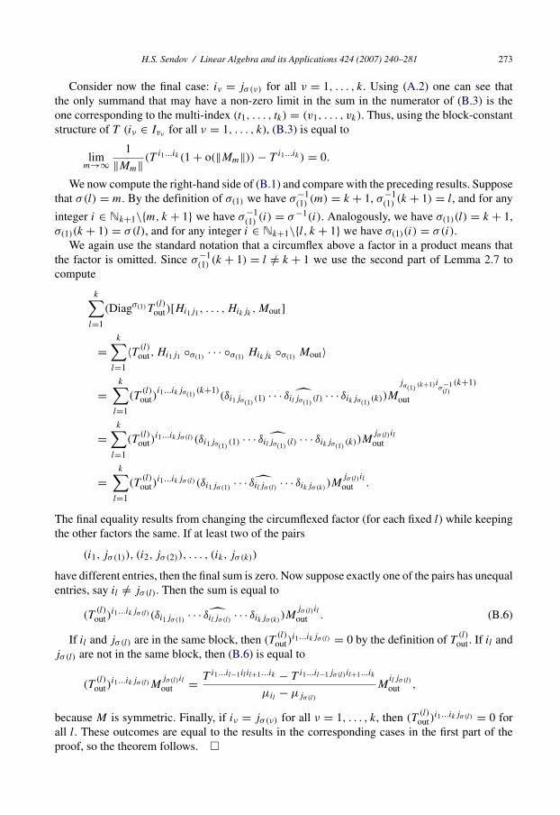
H.S. Sendov / Linear Algebra and its Applications 424 (2007) 240–281 273
Consider now the final case: iν = jσ(ν) for all ν = 1, . . . , k. Using (A.2) one can see thatthe only summand that may have a non-zero limit in the sum in the numerator of (B.3) is theone corresponding to the multi-index (t1, . . . , tk) = (v1, . . . , vk). Thus, using the block-constantstructure of T (iν ∈ Ivν for all ν = 1, . . . , k), (B.3) is equal to
limm→∞
1
‖Mm‖ (T i1...ik (1 + o(‖Mm‖)) − T i1...ik ) = 0.
We now compute the right-hand side of (B.1) and compare with the preceding results. Supposethat σ(l) = m. By the definition of σ(1) we have σ−1
(1) (m) = k + 1, σ−1(1) (k + 1) = l, and for any
integer i ∈ Nk+1\{m, k + 1} we have σ−1(1) (i) = σ−1(i). Analogously, we have σ(1)(l) = k + 1,
σ(1)(k + 1) = σ(l), and for any integer i ∈ Nk+1\{l, k + 1} we have σ(1)(i) = σ(i).We again use the standard notation that a circumflex above a factor in a product means that
the factor is omitted. Since σ−1(1) (k + 1) = l /= k + 1 we use the second part of Lemma 2.7 to
compute
k∑l=1
(Diagσ(1)T(l)out)[Hi1j1 , . . . , Hikjk
, Mout]
=k∑
l=1
〈T (l)out, Hi1j1 ◦σ(1)
· · · ◦σ(1)Hikjk
◦σ(1)Mout〉
=k∑
l=1
(T(l)out)
i1...ikjσ(1)(k+1)
(δi1jσ(1)(1) · · · δiljσ(1)
(l) · · · δikjσ(1)(k))M
jσ(1)(k+1)iσ−1
(l)
(k+1)
out
=k∑
l=1
(T(l)out)
i1...ikjσ(l) (δi1jσ(1)(1) · · · δiljσ(1)
(l) · · · δikjσ(1)(k))M
jσ(l)ilout
=k∑
l=1
(T(l)out)
i1...ikjσ(l) (δi1jσ(1)· · · δiljσ(l)
· · · δikjσ(k))M
jσ(l)ilout .
The final equality results from changing the circumflexed factor (for each fixed l) while keepingthe other factors the same. If at least two of the pairs
(i1, jσ(1)), (i2, jσ(2)), . . . , (ik, jσ(k))
have different entries, then the final sum is zero. Now suppose exactly one of the pairs has unequalentries, say il /= jσ(l). Then the sum is equal to
(T(l)out)
i1...ikjσ(l) (δi1jσ(1)· · · δiljσ(l)
· · · δikjσ(k))M
jσ(l)ilout . (B.6)
If il and jσ(l) are in the same block, then (T(l)out)
i1...ikjσ(l) = 0 by the definition of T(l)
out . If il andjσ(l) are not in the same block, then (B.6) is equal to
(T(l)out)
i1...ikjσ(l)Mjσ(l)ilout = T i1...il−1il il+1...ik − T i1...il−1jσ(l)il+1...ik
μil − μjσ(l)
Miljσ(l)
out ,
because M is symmetric. Finally, if iν = jσ(ν) for all ν = 1, . . . , k, then (T(l)
out)i1...ikjσ(l) = 0 for
all l. These outcomes are equal to the results in the corresponding cases in the first part of theproof, so the theorem follows. �

274 H.S. Sendov / Linear Algebra and its Applications 424 (2007) 240–281
Proposition B.2. Let T be any k + 1-tensor on Rn, let x ∈ Rn, let V be in On, and let σ be inP k. Then
V (Diagσ (T [x]))V T = (V (Diagσ(k+1)T )V T)[V (Diag x)V T].
Proof. Let Hi1j1 , . . . , Hikjkbe any k basic matrices. Since σ
(k+1)(i) = σ(i) for all i ∈ Nk and
σ(k+1)(k + 1) = k + 1, we can use Theorem 2.6 twice to compute
(V (Diagσ (T [x]))V T)i1 ...ikj1 ...jk = (V (Diagσ (T [x]))V T)[Hi1j1 , . . . , Hikjk
]= 〈T [x], Hi1j1 ◦σ . . . ◦σ Hikjk
〉
=n,...,n∑
p1,...,pk=1
(T [x])p1...pk Hp1pσ−1(1)
i1j1· · · H pkpσ−1(k)
ikjk
=n,...,n∑
p1,...,pk,pk+1=1
T p1...pk+1xpk+1Hp1pσ−1(1)
i1j1· · · H pkpσ−1(k)
ikjk
=n,...,n∑
p1,...,pk,pk+1=1
T p1...pk+1H
p1pσ−1(k+1)
(1)
i1j1· · · H
pkpσ−1(k+1)
(k)
ikjk(Diag x)
pk+1pσ−1(k+1)
(k+1)
= 〈T , Hi1j1 ◦σ(k+1). . . ◦σ(k+1)
Hikjk◦σ(k+1)
Diag x〉= (V (Diagσ(k+1)T )V T)[Hi1j1 , . . . , Hikjk
, V (Diag x)V T]= ((V (Diagσ(k+1)T )V T)[V (Diag x)V T])
i1 ...ikj1 ...jk .
Since the indices i1, . . . , ik and j1, . . . , jk are arbitrary we are done. �
The next lemma says that for any block-constant tensor T , Diagσ T is invariant under conju-gation with a block-diagonal orthogonal matrix.
Lemma B.3. Let T be a block constant k-tensor on Rn and let U ∈ On be a block diagonalmatrix (both with respect to the same partitioning of Nn). Then for any permutation σ in Nk
U(Diagσ T )UT = Diagσ T .
Proof. Let {I1, . . . , Ir}be the partitioning of the integers Nn that determines the block structure, soUipUjp = 0 whenever i � j or i � p, and
∑p∈Is
U ipUjp = δij whenever i ∈ Is . Let (i1, . . . , ik)be an arbitrary multi index and suppose that il ∈ Ivl
for l = 1, . . . , k. We expand the left-handside of the identity:
(U(Diagσ T )UT)i1 ...ikj1 ...jk =
n,...,n∑ps ,qs=1s=1,...,k
(Diagσ T )p1 ...pkq1 ...qk U i1p1Uj1q1 · · · UikpkUjkqk
=n,...,n∑
p1,...,pk=1
T p1...pkUi1p1Uj1pσ−1(1) · · · UikpkU
jkpσ−1(k)
=n,...,n∑
p1,...,pk=1
T p1...pkUi1p1Ujσ(1)p1 · · · UikpkUjσ(k)pk
H.S. Sendov / Linear Algebra and its Applications 424 (2007) 240–281 275
=r,...,r∑
t1,...,tk=1
T ιt1 ...ιtk∑pl∈Itl
l=1,...,k
U i1p1Ujσ(1)p1 · · · UikpkUjσ(k)pk
= T ιv1 ...ιvk∑
pl∈Ivll=1,...,k
U i1p1Ujσ(1)p1 · · · UikpkUjσ(k)pk
= T ιv1 ...ιvk δi1jσ(1)· · · δikjσ(k)
= T i1...ik δi1jσ(1)· · · δikjσ(k)
= (Diagσ T )i1 ...ikj1 ...jk .
The penultimate equality follows from the fact that T is block constant. �
Given a block structure on Nn and any matrix M , by Min we denote the matrix with the samediagonal blocks as M and the rest of the entries set to zero, as in (3).
Theorem B.4. Let U ∈ On be a block diagonal orthogonal matrix. Let M ∈ Sn be given and leth ∈ Rn be such that
UTMinU = Diag h. (B.7)
Let H1, . . . , Hk be arbitrary matrices and let σ be a permutation on Nk. Then
(i) for any block-constant (k + 1)-tensor T on Rn,
〈T [h], H1 ◦σ · · · ◦σ Hk〉 = 〈T , H1 ◦σ(k+1)· · · ◦σ(k+1)
Hk ◦σ(k+1)Min〉.
(ii) for any block-constant k-tensor T on Rn,
〈T τl [h], H1 ◦σ · · · ◦σ Hk〉 = 〈T (l)in , H1 ◦σ(1)
· · · ◦σ(1)Hk ◦σ(1)
Min〉 for all l = 1, . . . , k,
where the permutations σ(1) for l = 1, . . . , k, k + 1 are defined by (13), Hi = UTHiU fori = 1, . . . , k, and the lifting T τl is defined by (17).
Proof. To see that the first identity holds we use Theorem 2.6, Proposition B.2, (B.7), and LemmaB.3 in that order, as follows:
〈T [h], H1 ◦σ · · · ◦σ Hk〉 = (U(Diagσ T [h])UT)[H1, . . . , Hk]= (U(Diagσ
(k+1) T )UT)[H1, . . . , Hk, U(Diag h)UT]= (U(Diagσ
(k+1)T )UT)[H1, . . . , Hk, Min]= (Diagσ
(k+1) T )[H1, . . . , Hk, Min]= 〈T , H1 ◦σ(k+1)
· · · ◦σ(k+1)
Hk ◦σ(k+1)
Min〉.The final equality follows from Theorem 2.6.
To show the second identity, it suffices to prove it for arbitrary basic matrices Hisjs s = 1, . . . , k.Fix k basic matrices Hi1j1 , . . . , Hikjk
and suppose that il ∈ Ivlfor l = 1, . . . , k. Then
〈T τl [h], Hi1j1 ◦σ · · · ◦σ Hikjk〉
= (U(Diagσ T τl [h])UT)[Hi1j1 , . . . , Hikjk]

276 H.S. Sendov / Linear Algebra and its Applications 424 (2007) 240–281
= (U(Diagσ T τl [h])UT)i1 ...ikj1 ...jk
=n,...,n∑
p1,...,pk=1q1,...,qk=1
(Diagσ T τl [h]) p1 ...pkq1 ...qk U i1p1Uj1q1 · · · UikpkUjkqk
=n,...,n∑
p1,...,pk=1
(T τl [h])p1...pkUi1p1Uj1pσ−1(1) · · · UikpkU
jkpσ−1(k)
=n,...,n∑
p1,...,pk=1
(T τl [h])p1...pkUi1p1Ujσ(1)p1 · · · UikpkUjσ(k)pk
=n,...,n∑
p1,...,pk=1
n∑pk+1=1
(T τl )p1...pkpk+1hpk+1Ui1p1Ujσ(1)p1 · · · UikpkUjσ(k)pk
=n,...,n∑
p1,...,pk=1
T p1...pkhplUi1p1Ujσ(1)p1 · · · UikpkUjσ(k)pk
=r,...,r∑
t1,...,tk=1
T ιt1 ...ιtk∑
pη∈Itηη=1,...,k
hplUi1p1Ujσ(1)p1 · · · UikpkUjσ(k)pk
= T ιv1 ...ιvk∑
pl∈Ivll=1,...,k
hplUi1p1Ujσ(1)p1 · · · UikpkUjσ(k)pk
= T ιv1 ...ιvk δi1jσ(1)· · · δiljσ(l)
· · · δikjσ(k)
∑pl∈Ivl
hplUilplUjσ(l)pl
= T i1...ik δi1jσ(1)· · · δiljσ(l)
· · · δikjσ(k)
∑pl∈Ivl
hplUilplUjσ(l)pl
= T i1...ik δi1jσ(1)· · · δiljσ(l)
· · · δikjσ(k)M
iljσ(l)
in .
To evaluate the right-hand side of the identity, we use the second part of Lemma 2.7 sinceσ−1
(l)(k + 1) = l /= k + 1. Since σ
(l)(s) = σ(s) for s ∈ Nk+1\{l, k + 1} and σ
(l)(k + 1) = σ(l)
for all l = 1, . . . , k, we can calculate
〈T (l)in , Hi1j1 ◦σ
(l)· · · ◦σ
(l)Hikjk
◦σ(l)
Min〉
= (T(l)in )
i1...ikjσ(l)
(k+1)δi1jσ
(l)(1)
· · · δiljσ(l)
(l)· · · δikjσ
(l)(k)
M
jσ(l)
(k+1)iσ−1(l)
(k+1)
in
= (T(l)in )i1...ikjσ(l) δi1jσ(1)
· · · δiljk+1 · · · δikjσ(k)M
jσ(l)ilin
= T i1...ik δi1jσ(1)· · · δiljk+1 · · · δikjσ(k)
Mjσ(l)ilin
= T i1...ik δi1jσ(1)· · · δiljk+1 · · · δikjσ(k)
Miljσ(l)
in
= T i1...ik δi1jσ(1)· · · δiljσ(l)
· · · δikjσ(k)M
iljσ(l)
in .
H.S. Sendov / Linear Algebra and its Applications 424 (2007) 240–281 277
In the third equality we used the fact that T is block constant, as well as the fact that Mjσ(l)ilin = 0
if jσ(l) � il . In the fourth equality we used the fact that M is symmetric. The final equality holdsbecause we changed the missing factor, while keeping the other factors the same. �
Proposition B.5. Let U ∈ On be block diagonal, let H be an n × n matrix, and let σ be anypermutation on Nk.
(i) If T is a (k + 1)-tensor such that for some fixed l ∈ Nk we have T p1...pl ...pk+1 = 0 wheneverpl ∼ pk+1, then
(U(Diagσ(l) T )UT)[Hin] = 0.
(ii) If T is a (k + 1)-tensor such that for some fixed l ∈ Nk we have T p1...pl ...pk+1 = 0 wheneverpl � pk+1, then
(U(Diagσ(l) T )UT)[Hout] = 0.
(iii) If T is any (k + 1)-tensor, then
(U(Diagσ(k+1) T )UT)[Hout] = 0.
Proof. Fix an index l in Nk . Let Hi1j1 , . . . , Hikjkbe arbitrary basic matrices, and let H be an
arbitrary matrix. Using the definitions we compute
(U(Diagσ(l) T )UT)[Hi1j1 , . . . , Hikjk
, H ]
=n,n∑
ik+1,jk+1=1
(U(Diagσ(l) T )UT)
i1 ...ik+1j1 ...jk+1 Hik+1jk+1
=n,n∑
ik+1,jk+1=1
n,...,n∑ps ,qs=1
s=1,...,k+1
(Diagσ(l) T )
p1 ...pk+1q1 ...qk+1 Ui1p1Uj1q1 · · · Uik+1pk+1Ujk+1qk+1Hik+1jk+1
=n,n∑
ik+1,jk+1=1
n,...,n∑ps=1
s=1,...,k+1
T p1...pk+1Ui1p1Uj1p
σ−1(l)
(1) · · · Uik+1pk+1Ujk+1p
σ−1(l)
(k+1)H ik+1jk+1
=n,n∑
ik+1,jk+1=1
n,...,n∑ps=1
s=1,...,k+1
(T p1...pk+1Ui1p1U
jσ(l)
(1)p1 · · · UilplU
jσ(l)
(l)pl
· · · Uik+1pk+1Ujσ(l)
(k+1)pk+1
Hik+1jk+1)
=n,n∑
ik+1,jk+1=1
n,...,n∑ps=1
s=1,...,k+1
(T p1...pk+1Ui1p1Ujσ(1)p1 · · · UilplUjk+1pl
· · · Uik+1pk+1Ujσ(l)pk+1Hik+1jk+1).
Now suppose that T is a (k + 1)-tensor with T p1...pl ...pk+1 = 0 whenever pl ∼ pk+1 and thatH = Hin. Then Hik+1jk+1 /= 0 implies that ik+1 ∼ jk+1. In that case, by the fact that U is blockdiagonal, Ujk+1plUik+1pk+1 /= 0 implies that pl ∼ pk+1, which implies that T p1...pl ...pk+1 = 0.Thus every summand in the final double sum is zero.
278 H.S. Sendov / Linear Algebra and its Applications 424 (2007) 240–281
In the second case, suppose T is a (k + 1)-tensor with T p1...pl ...pk+1 = 0 whenever pl � pk+1and H = Hout. Then Hik+1jk+1 /= 0 implies that ik+1 � jk+1. In that case, by the fact that U is blockdiagonal, Ujk+1plUik+1pk+1 /= 0 implies that pl � pk+1, which implies that T p1...pl ...pk+1 = 0. Thesum is zero.
In the third case, suppose that T is any (k + 1)-tensor and H = Hout. A calculation almostidentical to the one at the beginning of the proof (it differs only in the last step) shows that
(U(Diagσ(k+1) T )UT)[Hi1j1 , . . . , Hikjk
, H ]
=n,n∑
ik+1,jk+1=1
n,...,n∑ps=1
s=1,...,k+1
T p1...pk+1Ui1p1Ujσ(1)p1
· · · UikpkUjσ(k)pkUik+1pk+1Ujk+1pk+1Hik+1jk+1 .
Then Hik+1jk+1 /= 0 implies that ik+1 � jk+1. In that case, by the fact that U is block diagonal,Ujk+1pk+1Uik+1pk+1 = 0. Again the sum is zero. �
We are finally ready to conclude the proofs of our two main analytical tools.
Proof of Theorem 9. A consequence of Theorem B.1 and Proposition B.5. �
Proof of Theorem 10. A consequence of Theorem 2.6, Theorem B.4, Proposition B.5, and thefact that M = Min + Mout. �
If vector μ defining the equivalence relation on Nn has distinct entries, then every tensor fromT k,n is block constant and the block-diagonal orthogonal matrices are precisely the signed identitymatrices (those with plus or minus one on the main diagonal and zeros everywhere else). In thiscase we also have i ∼ j if and only if i = j and thus T
(l)in = T τl . Moreover, since Proposition B.5
holds for arbitrary matrices (symmetric or not), Theorem 2.10 implies the next corollary, validfor an arbitrary matrix H .
Corollary B.6. Let σ be a permutation on Nk and let H be an arbitrary matrix. Then
(i) for any (k + 1)-tensor T on Rn,
Diagσ (T [diag H ]) = (Diagσ(k+1) T )[H ];
(ii) for any k-tensor T on Rn
Diagσ (T τl [diag H ]) = (Diagσ(l) T τl )[H ] for all l = 1, . . . , k,
where the permutations σ(l)
, for l ∈ Nk, are defined by (13).
Appendix C. Proof of Theorem 6.4
Let X ∈ Sn have distinct eigenvalues, and let x = λ(X). The proof of Theorem 6.4 is by induc-tion on s. When s = 1 there is nothing to show since by definition A
(1)(x) = ∇f (x) = A
(1)(x)
for every x ∈ Rn. Suppose that for some integer s in [1, k) we have
H.S. Sendov / Linear Algebra and its Applications 424 (2007) 240–281 279∑σ∈P s
DiagσAσ (x) =∑σ∈P s
DiagσAσ (x),
for every x ∈ Rn with distinct entries.By definition, the tensor Aσ (x) is equal to zero if the permutation σ has more than one cycle
in its cycle decomposition. Then using Lemma 6.3 gives∑σ∈P s+1
DiagσAσ (x) =∑σ∈Ps
l∈Ns+1
Diagσ(1)Aσ(1)(x)
=∑σ∈Ps
l∈Ns
Diagσ(1)Aσ(1)(x)
=∑σ∈Ps
l∈Ns
Diagσ(1) ((Aσ (x))(l)out + (T l
σ (x))(l)in ).
Let M ∈ §n and suppose ‖M‖ = 1. Let {Mm}∞m=1 be a sequence of symmetric matrices convergingto zero and such that Mm/‖Mm‖ converges to M . Finally, let {Um}∞m=1 be a sequence of orthogonalmatrices such that
Diag x + Mm = Um(Diag λ(Diag x + Mm))UTm.
By taking a subsequence if necessary, we may assume that Um converges to U ∈ On when m
goes to infinity. Since the partition of the integers Nn into blocks is determined by the repeatedeigenvalues of the matrix X, and the latter are all distinct, we have Min = Diag (diag M). (More-over, every tensor is block constant.) Thus, defining h ∈ Rn as in (23) we see that h = diag M
and by (25) we have UTMinU = Diag (diag M). on the one hand, the induction hypothesis andthe first part of Theorem 2.10 give⎛⎜⎝∑
σ∈Ps
l∈Ns
Diagσ(1) (T lσ (x))
(l)in
⎞⎟⎠ [M]
= U
(∑σ∈P s
Diagσ (∇Aσ (x)[h]))
UT
= limt→0
U
(∑σ∈P s
Diagσ (Aσ (x + th) − Aσ (x))
)UT
= limt→0
U
(∑σ∈P s
Diagσ (Aσ (x + th) − Aσ (x))
)UT
= U
(∑σ∈P s
Diagσ (∇Aσ (x)[h]))
UT
=(∑
σ∈P s
Diagσ(s+1)∇Aσ (x)
)[M]
=(∑
σ∈P s
Diagσ(s+1)Aσ(s+1)(x)
)[M].
280 H.S. Sendov / Linear Algebra and its Applications 424 (2007) 240–281
In the final equality we used the second line from (28). On the other hand, using (15), the inductionhypothesis, and again (15) we have⎛⎜⎝∑
σ∈Ps
l∈Ns
Diagσ(1) (Aσ (x))(l)out
⎞⎟⎠ [M]
= limm→∞
Um(∑
σ∈P s DiagσAσ (x))UTm −∑
σ∈P s DiagσAσ (x)
‖Mm‖= lim
m→∞Um(
∑σ∈P s DiagσAσ (x))UT
m −∑σ∈P s DiagσAσ (x)
‖Mm‖
=⎛⎜⎝∑
σ∈Ps
l∈Ns
Diagσ(1) (Aσ (x))(l)out
⎞⎟⎠ [M]
=⎛⎜⎝∑
σ∈Ps
l∈Ns
Diagσ(1)Aσ(1)(x)
⎞⎟⎠ [M].
In the final equality we used the first line in (28). Thus we see that⎛⎝ ∑σ∈P s+1
DiagσAσ (x)
⎞⎠ [M] =⎛⎝ ∑
σ∈P s+1
DiagσAσ (x)
⎞⎠ [M],
and since M was arbitrary, we are done.
Acknowledgments
I thank Jérôme Malick for his interest in this work, and for informing me about several typos inthe earlier versions of the manuscript. I especially thank the first referee for his thorough reading,invaluable help, and guidance in bringing up the manuscript to its current state. Finally, I thankHeinz Bauschke and Adrian Lewis for their support and encouragement.
References
[1] V.I. Arnold, On matrices depending on parameters, Russian Math. Surveys 26 (1971) 29–43.[2] R. Bhatia, Matrix Analysis, Springer-Verlag, NY, 1997.[3] X. Chen, H.-D. Qi, P. Tseng, Analysis of nonsmooth symmetric matrix functions with applications to semidifinite
programming, SIAM J. Optim. 13 (2003) 960–985.[4] Yu.L. Daleckii, Integration and differentiation of functions of Hermitian operators depending on a parameter, Amer.
Math. Soc. Transl. Ser. 2 16 (1960) 396–400.[5] Yu.L. Daleckii, S.G. Krein, Formulas of differentiation according to a parameter of functions of Hermitian operators,
Dokl. Akad. Nauk SSSR (N.S.) 76 (1951) 13–16.[6] W.F. Donoghue, Monotone Matrix Functions and Analytic Continuation, Die Grundlehren der mathematischen
Wissenschaften, Band 207, Springer-Verlag, New York–Heidelberg, 1974.[7] J.-B. Hiriart-Urruty, D. Ye, Sensitivity analysis of all eigenvalues of a symmetric matrix, Numer. Math. 70 (1992)
45–72.[8] R.A. Horn, C.R. Johnson, Topics in Matrix Analysis, Cambridge University Press, 1994 (first paperback edition
with corrections).

H.S. Sendov / Linear Algebra and its Applications 424 (2007) 240–281 281
[9] T. Kato, Perturbation Theory for Linear Operators, Grundlehren der Mathematischen Wissenschaften Band 132,second ed., Springer-Verlag, New York, Berlin, 1976.
[10] E.C. Kemble, The Fundamental Principles of Quantum Mechanics, Dover, New York, 1958.[11] F. Kraus, Über Konvexe Matrixfunctionen, Math. Z. 41 (1) (1936) 18–42.[12] A.S. Lewis, Convex analysis on the Hermitian matrices, SIAM J. Optim. 6 (1996) 164–177.[13] A.S. Lewis, Derivatives of spectral functions, Math. Oper. Res. 21 (1996) 576–588.[14] A.S. Lewis, Nonsmooth analysis of eigenvalues, Math. Program. 84 (1999) 1–24.[15] A.S. Lewis, The mathematics of eigenvalue optimization, Math. Program. Ser. B 97 (1–2) (2003) 155–176.[16] A.S. Lewis, M.L. Overton, Eigenvalue optimization, Acta Numer. 5 (1996) 149–190.[17] A.S. Lewis, H.S. Sendov, Twice differentiable spectral functions, SIAM J. Matrix Anal. Appl. 23 (2) (2001) 368–386.[18] A.S. Lewis, H.S. Sendov, Quadratic expansions of spectral functions, Linear Algebra Appl. 340 (2002) 97–121.[19] K. Löwner, Über Monotone Matrixfunctionen, Math. Z. 38 (1) (1934) 177–216.[20] J. Malick, H.S. Sendov, Clarke generalized Jacobian of the projection onto the cone of positive semidefinite matrices,
Set-Valued Anal. 14 (3) (2006) 273–293.[21] R. Mathias, A chain rule for matrix functions and applications, SIAM J. Matrix Anal. Appl. 17 (3) (1996) 610–620.[22] H.S. Sendov, Generalized Hadamard product and the derivatives of spectral functions, SIAM J. Matrix Anal. Appl.
28 (3) (2006) 667–681.[23] D. Sun, J. Sun, Semismooth matrix-valued functions, Math. Oper. Res. 27 (1) (2002) 150–169.[24] N.-K. Tsing, M.K.H. Fan, E.I. Verriest, On analyticity of functions involving eigenvalues, Linear Algebra Appl. 207
(1994) 159–180.