The Harrod-Balassa-Samuelson Effect: Reconciling the Evidence · Preliminary version Please do not quote without permission The Harrod-Balassa-Samuelson Effect: Reconciling the Evidence

Preliminary version Please do not quote

without permission

The Harrod-Balassa-Samuelson Effect:

Reconciling the Evidence

Christiane Baumeister

Ehsan U. Choudhri

Lawrence L. Schembri

International Economic Analysis Department

Bank of Canada

Economics Department

Carleton University

11 June 2011

The authors would like to David Finer and Golbahar Kazemian for excellent research assistance. The

views expressed in this paper are those of the authors and should not be attributed to the Bank of Canada.

1

1. Introduction

Many emerging market countries have experienced rapid growth over the past two

decades driven, in part, by large increases in productivity growth. This growth has also been

accompanied by a real exchange rate appreciation. These developments have recently spurred a

renewed interest in the Harrod-Balassa-Samuelson (HBS) hypothesis concerning the effect of

productivity changes on the real exchange rate.1 The systematic empirical evidence surrounding

the HBS hypothesis is, however, mixed.2

Most empirical models are based on simplified versions of the conventional HBS model,

which identifies the price ratio of non-tradable goods to tradable goods as the key relative price

through which relative productivity changes in the tradables and non-tradables influence the real

exchange rate. We test this model, using a panel data set of 16 OECD countries over 30 years.

The time series properties of the panel are examined to test for unit roots and co-integration in

order to develop and to implement the appropriate empirical model and econometric

methodology. The strength of our empirical approach is that the regression model is derived

directly from a theoretical model and therefore permits a theoretical interpretation of our

empirical results.

Our key empirical findings are: the estimates of the impacts of tradable and non-tradable

productivity differentials on the real exchange rate are heterogeneous across countries and

sensitive to the choice of the reference country (U.S., Germany, and the average of the other

countries in the panel). In most cases, the effect of an increase in tradable productivity in the

home country relative to the base country is statistically significant and causes the real exchange

1 Harrod (1933), Balassa (1964) and Samuelson (1964).

2 Peltonen and Sager (2009) provide a recent survey of the HBS empirical literature.

2

rate to depreciate, while the non-tradables productivity differential has, on average, the opposite

effect of appreciating the real exchange, but is not that significant and smaller in absolute

magnitude than the theory would predict. The signs of the average effect of the tradable and non-

tradable productivity differentials are opposite of what the HBS hypothesis would predict. These

mixed results are similar to others found in the literature.3

The other important contribution of the paper is to explore whether these different

empirical results can be reconciled with the HBS model and to obtain a deeper understanding of

the theoretical underpinnings of these findings. To this end, we first derive a conventional

version of the HBS model and then extend it by introducing monopolistic competition with

symmetric firms and free entry (e.g., Krugman, 1980). In this model, productivity effects also

operate through the relative price of home to foreign varieties of tradables (the terms of trade)

and the number of firms in the tradable relative to the non-tradable sectors, in addition to the

conventional HBS channel through the relative price of non-tradables.4 It is well known that the

adjustment in the terms of trade can weaken or even reverse the effect of the tradable

productivity differential on the real exchange rate.5 However, the influence of terms of trade

adjustment on the effect of non-tradable productivity differential and the implications of changes

in the number of firms on the effects of both productivity differentials have not been fully

explored. We examine these questions within the HBS model extended to incorporate

monopolistic competition. Our analytical solution of the model indicates that both the elasticity

3 Peltonen and Sager (2009) find similar inconsistent results using data starting in 1990 with a larger sample of

advanced and emerging market economies. 4 Recent developments in the monopolistic-competition models (Melitz, 2003) allow productivity to be

heterogeneous across firms. Melitz and Ghironi (2005) use a one-sector model with heterogeneous firms to show

that productivity improvement across all firms exerts an effect on the real exchange rate, which is similar to the

conventional Harrod-Balassa-Samuelson effect and operates via the relative price of exported varieties. 5For example, in a DGE models of an open economy (calibrated to UK-Euro area) with fixed number of firms,

Benigno and Thoenissen (2003) find that an increase in the tradable productivity in the U.K. causes a sufficient

deterioration in the U.K. terms of trade to lead to a decrease in the real value of the pound.

3

of substitution between home and foreign tradable goods and that between tradables and non-

tradables play an important role in determining the effects of the two productivity differentials.6

Our results show that the effect of each differential can be reversed if the home-foreign goods

elasticity of substitution is sufficiently low and the domestic tradable-non-tradable substitution

elasticity is sufficiently high. Our numerical analysis of the model calibrated to an average

OECD country shows that a low value of the former elasticity close to 0.5 and a high value of the

latter elasticity close to 3 can explain the unexpected signs of the effects of the tradable and

nontradable productivity differentials on the real exchange rate.

The extended theoretical model does not, however, provide a full explanation of the

cross-country heterogeneity and the sensitivity of the results to different specifications. Like

Peltonen and Sager (2009), we find that the empirical results are sensitive to the specification of

the empirical model and the data used. Fragility of the empirical results might also be associated

with the definition of the productivity measure employed in the analysis.7 Another concern

relates to the fact that the sample might not be sufficiently long for low-frequency estimation of

these long-run HBS parameters and thus the estimation cannot adequately purge the impact of

business cycle and other short-to-medium-run macroeconomic effects. In other words, to find

evidence consistent with the HBS hypothesis either requires very long samples or significant

differences in productivity growth.8 The most robust evidence for advanced countries is that by

Lothian and Taylor (2008) who use almost two centuries of data on per capita income and the

real exchange rate for the United States and United Kingdom. For emerging market economies,

6 Choudhri and Schembri (2010) highlight the role of the elasticity of substitution between home and foreign

tradable goods in the transmission of productivity changes to the terms of trade and the real exchange rate. 7 Lee and Tang (2007) note that their results are sensitive to the definition of productivity (total factor versus labour

productivity). 8 This finding is similar to that found for relative purchasing power parity: namely to explain movements in

nominal exchange rates by inflation differentials normally requires a large cumulative differential - obtained either

with a very large average differential over a short sample or a small average differential over a long sample.

4

the strongest recent evidence consistent with the HBS hypothesis has been found for Central and

Eastern European countries (Freeman, 2008; Mihaljek and Blau, 2008).

In the next section, we develop the theoretical framework that provides the basis for our

empirical model. In section 3, we describe the panel database, perform unit root and co-

integration tests to examine the time series properties of the data and estimate the empirical

model using dynamic OLS (DOLS). The final two sections attempt to interpret the empirical

results within the theoretical framework provided in section 2 and outline plans for future work.

2. Theoretical Framework

This section uses a simple framework to examine how the introduction of monopolistic

competition in the HBS model influences the effects of productivity changes on the real

exchange rate. We use a simple setup with two countries (home and foreign), one factor (labor),

and two composite goods (representing sectors with tradable and non-tradable goods). To focus

on long-run effects, we assume flexible prices and financial autarky.9 In this setup, we first

briefly review the conventional Harrod-Balassa-Samuelson model with perfect competition and

diversified production for tradables (all goods in the tradable sector can be produced in both

countries). We then extend the model to incorporate monopolistic competition and examine how

this extension modifies the relations implied by the conventional model.

2.1 Conventional Model

To develop the conventional model for the HBS hypothesis, we first examine the

equations of for the home economy. Symmetric equations are assumed for the foreign economy

9 The solution of the model under these assumptions would duplicate the steady-state solution of a dynamic model

with nominal rigidities, where net foreign assets converge to zero in the long run.

5

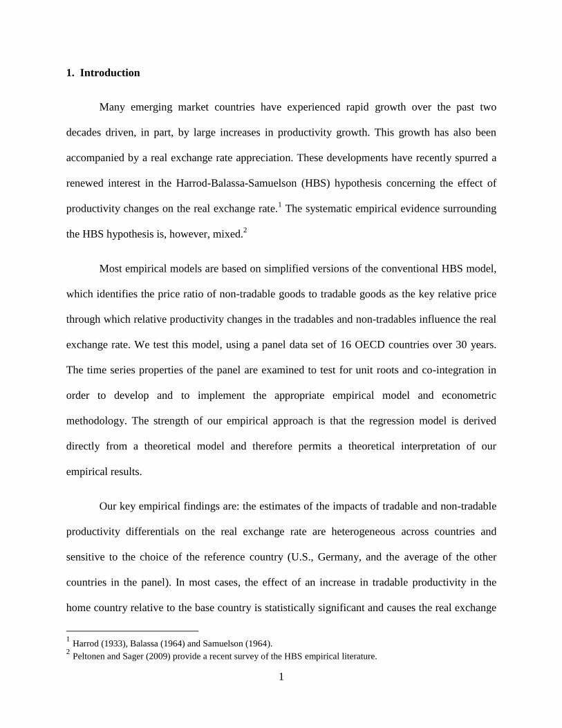
with an asterisk used to denote foreign variables and parameters. To facilitate comparison with

the monopolistic-competition model discussed below, we assume CES aggregators and a

continuum of goods in tradable and non-tradable bundles. Letting C denote the household’s

aggregate consumption index, we define it as

/( 1)

1/ ( 1)/ 1/ ( 1)/(1 )N TC C C

, (1)

where NC and TC represent the consumption of composite non-tradable and tradable goods, and

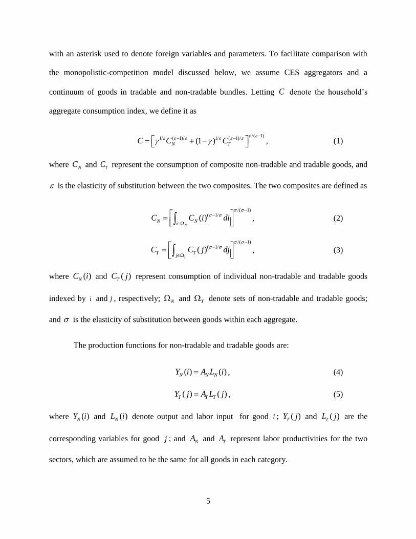
is the elasticity of substitution between the two composites. The two composites are defined as

/( 1)

( 1/( )N

N Ni

C C i di

, (2)

/( 1)

( 1/( )T

T Tj

C C j dj

, (3)

where ( )NC i and ( )TC j represent consumption of individual non-tradable and tradable goods

indexed by i and j , respectively; N and T denote sets of non-tradable and tradable goods;

and is the elasticity of substitution between goods within each aggregate.

The production functions for non-tradable and tradable goods are:

( ) ( )N N NY i A L i , (4)

( ) ( )T T TY j A L j , (5)

where ( )NY i and ( )NL i denote output and labor input for good i ; ( )TY j and ( )TL j are the

corresponding variables for good j ; and NA and TA represent labor productivities for the two

sectors, which are assumed to be the same for all goods in each category.

6

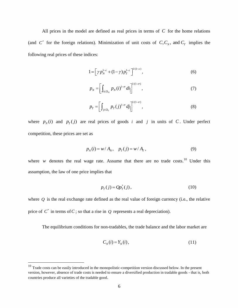
All prices in the model are defined as real prices in terms of C for the home relations

(and *C for the foreign relations). Minimization of unit costs of , , and N TC C C implies the

following real prices of these indices:

1/(1 )

1 11 (1 )N Tp p

, (6)

1/(1 )

1( )N

N Ni

p p i di

, (7)

1/(1 )

1( )T

T Tj

p p j dj

, (8)

where ( )Np i and ( )Tp j are real prices of goods i and j in units of C . Under perfect

competition, these prices are set as

( ) / , ( ) /N N T Tp i w A p j w A , (9)

where w denotes the real wage rate. Assume that there are no trade costs.10

Under this

assumption, the law of one price implies that

*( ) ( )T Tp j Qp j , (10)

where Q is the real exchange rate defined as the real value of foreign currency (i.e., the relative

price of *C in terms ofC ; so that a rise in Q represents a real depreciation).

The equilibrium conditions for non-tradables, the trade balance and the labor market are

( ) ( )N NC i Y i , (11)

10

Trade costs can be easily introduced in the monopolistic-competition version discussed below. In the present

version, however, absence of trade costs is needed to ensure a diversified production in tradable goods - that is, both

countries produce all varieties of the tradable good.

7

( )[ ( ) ( )] 0T

T T Tj

p j C j Y j dj

, (12)

( ) ( )N T

N Ti j

L L i di L j dj

, (13)

where L is the fixed supply of labour.

To solve for the response of the real exchange rate to productivity changes, we use a first-

order log-linear approximation around the initial state. We let initial values of Tp and Np equal

to one by normalization, so that represents the share of non-tradables in aggregate

consumption in the initial state. To simplify the form of the real exchange rate relation derived

below, we assume that this share is homogeneous across countries. Letting a hat over a variable

denote the log deviation from its initial value, setting* , and using (6)-(8), their foreign

counterparts and (10), we first express

* *ˆ ˆ ˆ ˆ ˆ( ) ( )N T N TQ p p p p (14)

Next, letting ˆ ˆˆ ˆN T T Np p A A and

* * * *ˆ ˆˆ ˆN T T Np p A A from (7)-(9) and their foreign

counterparts, we relate the real exchange rate to home-foreign productivity differentials for

tradables and non-tradables as

* *ˆ ˆ ˆ ˆ ˆ( ) ( )T T N NQ A A A A . (15)

This relation represents a typical form of the Harrod-Balassa-Samuelson relation for the

real exchange rate. The HBS hypothesis is typically interpreted to presume that productivity

growth in non-tradables is zero or the differential in the non-tradable sector is small so that the

productivity growth differential in tradables explains the bulk of the movements in the real

exchange rate. For example, a sharp increase in productivity growth in the home country will

8

cause a real appreciation of home currency (a decrease in Q ) as economy wide wages increase

and the relative price of domestic to foreign non-tradables rise.

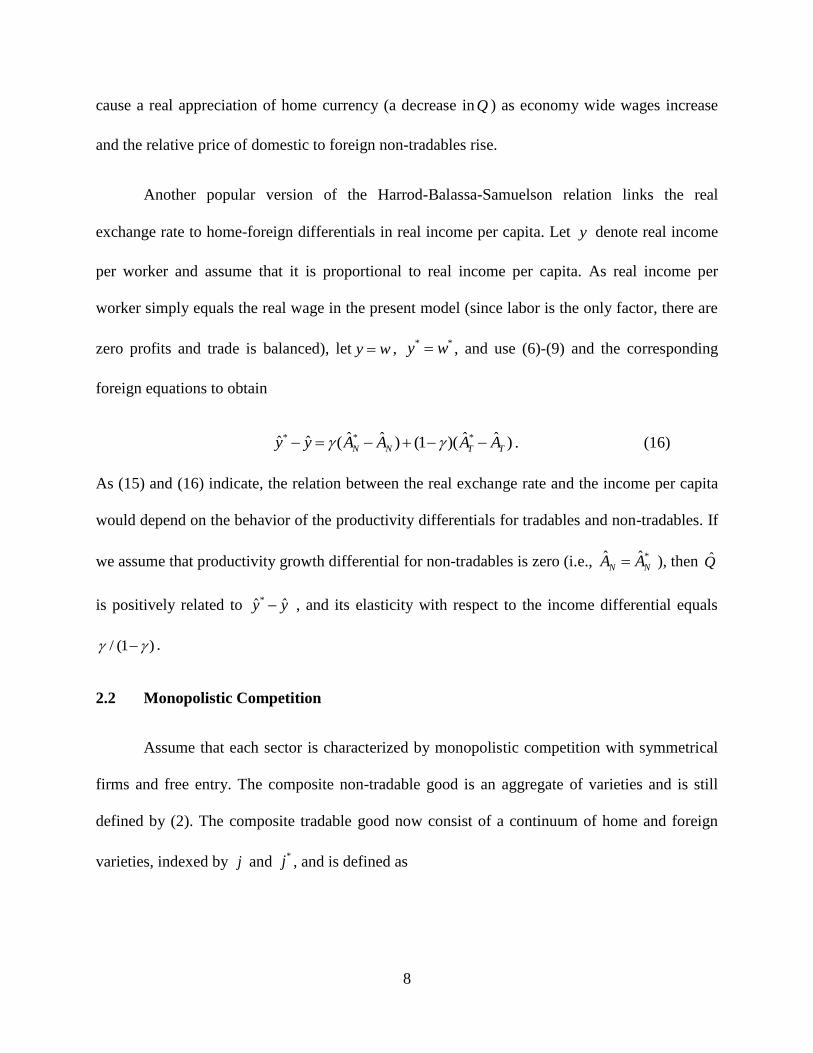
Another popular version of the Harrod-Balassa-Samuelson relation links the real

exchange rate to home-foreign differentials in real income per capita. Let y denote real income

per worker and assume that it is proportional to real income per capita. As real income per

worker simply equals the real wage in the present model (since labor is the only factor, there are

zero profits and trade is balanced), let y w , * *y w , and use (6)-(9) and the corresponding

foreign equations to obtain

* * *ˆ ˆ ˆ ˆˆ ˆ ( ) (1 )( )N N T Ty y A A A A . (16)

As (15) and (16) indicate, the relation between the real exchange rate and the income per capita

would depend on the behavior of the productivity differentials for tradables and non-tradables. If

we assume that productivity growth differential for non-tradables is zero (i.e., *ˆ ˆ

N NA A ), then Q̂

is positively related to *ˆ ˆy y , and its elasticity with respect to the income differential equals

/ (1 ) .

2.2 Monopolistic Competition

Assume that each sector is characterized by monopolistic competition with symmetrical

firms and free entry. The composite non-tradable good is an aggregate of varieties and is still

defined by (2). The composite tradable good now consist of a continuum of home and foreign

varieties, indexed by j and *j , and is defined as

9

*

/( 1)1/ ( 1)/ 1/ ( 1)/

/( 1) /( 1)( 1)/ * ( 1)/ *

(1 ) ,

( ) , ( ) ,H F

T H F

H H F Fj j

C C C

C C j dj C C j dj

(17)

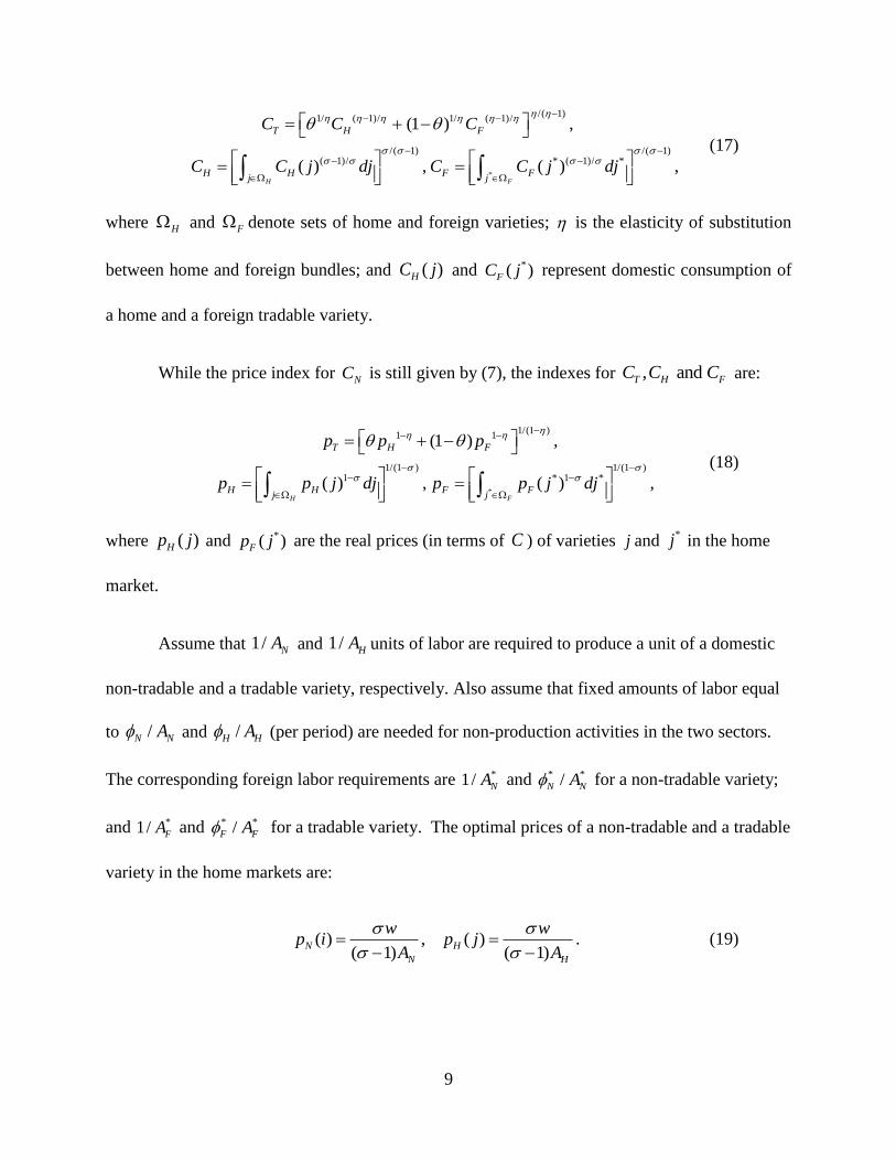
where H and F denote sets of home and foreign varieties; is the elasticity of substitution

between home and foreign bundles; and ( )HC j and *( )FC j represent domestic consumption of

a home and a foreign tradable variety.

While the price index for NC is still given by (7), the indexes for , and T H FC C C are:

*

1/(1 )1 1

1/(1 ) 1/(1 )1 * 1 *

(1 ) ,

( ) , ( ) ,H F

T H F

H H F Fj j

p p p

p p j dj p p j dj

(18)

where ( )Hp j and *( )Fp j are the real prices (in terms of C ) of varieties j and *j in the home

market.

Assume that 1/ NA and 1/ HA units of labor are required to produce a unit of a domestic

non-tradable and a tradable variety, respectively. Also assume that fixed amounts of labor equal

to /N NA and /H HA (per period) are needed for non-production activities in the two sectors.

The corresponding foreign labor requirements are *1/ NA and * */N NA for a non-tradable variety;

and *1/ FA and * */F FA for a tradable variety. The optimal prices of a non-tradable and a tradable

variety in the home markets are:

( ) , ( )( 1) ( 1)

N H

N H

w wp i p j

A A

. (19)

10

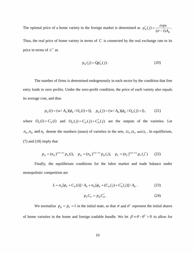
The optimal price of a home variety in the foreign market is determined as * ( ) .( 1)

H

H

qwp j

A

Thus, the real price of home variety in terms of C is connected by the real exchange rate to its

price in terms of *C as

*( ) ( )H Hp j Qp j . (20)

The number of firms is determined endogenously in each sector by the condition that free

entry leads to zero profits. Under the zero-profit condition, the price of each variety also equals

its average cost, and thus

( ) ( / )( / ( ) 1), ( ) ( / )( / ( ) 1)N N N N H H H Hp i w A O i p j w A O j , (21)

where ( ) ( )N NO i C i and *( ) ( ) ( )H H HO j C j C j are the outputs of the varieties. Let

, and N H Fn n n denote the numbers (mass) of varieties in the sets, , and N H F . In equilibrium,

(7) and (18) imply that

1/(1 ) 1/(1 ) 1/(1 ) *( ) ( ), ( ) ( ), ( ) ( )N N N H H H F F Fp n p i p n p j p n p j (22)

Finally, the equilibrium conditions for the labor market and trade balance under

monopolistic competition are

*[ ( )] / [ ( ( ) ( )] /N N N N H H H H HL n C i A n C j C j A . (23)

*

F F H Hp C p C . (24)

We normalize 1H Fp p in the initial state, so that * and represent the initial shares

of home varieties in the home and foreign tradable bundle. We let * 0 to allow for

11

home bias. Then, letting /H Fp p denote the terms of trade, and noting that * */ /H F H Fp p p p

in view of (20) and its foreign counterpart, we use (6), (7), (18) and (20) to derive the real

exchange rate relation as * *ˆ ˆ ˆ ˆ ˆ ˆ( ) ( )N T N TQ p p p p . Thus, in addition to the price

differential for non-tradables and tradables, the real exchange rate also depends on the terms of

trade in the presence of home bias. Another important difference from the conventional model is

that the price differentials are now related to the terms of trade and the number of varieties in

each sector. Using (19), (22), and the corresponding foreign relations, we can express

ˆ ˆˆ ˆ ˆ ˆ ˆ(1 ) ( ) / ( 1)N T H N H Np p A A n n and

* * * * * *ˆ ˆˆ ˆ ˆ ˆ ˆ( ) / ( 1)N T F N H F Np p A A n n .

Substituting these expressions for price differentials in the above exchange rate relation, we

obtain

* *ˆ ˆ ˆ ˆ ˆ ˆˆ( ) ( ) [ (1 ) ] [ / ( 1)] ,F H N NQ A A A A (25)

where *ˆ ˆ ˆ ˆ ˆ( )F N H Nn n n n is an index based on the difference between foreign and home

economies in the number of non-tradable relative to tradable varieties.

In the real exchange rate relation (25), the productivity differentials affect the exchange

rate directly as well as indirectly via the terms of trade and the variety index. To examine the

indirect effects, the model is solved in the Appendix to determine

* *(1 ) ( 1)ˆ ˆ ˆ ˆˆ ( ) ( )( 1) ( 1)

F H N NA A A A

(26)

* *(1 ) ( 1)ˆ ˆ ˆ ˆˆ 1 ( ) 1 ( )F H N NA A A A

(27)

where 1 (1 )(1 ) (1 ) , ( 1) / ( ) , and / (1 ) .

12

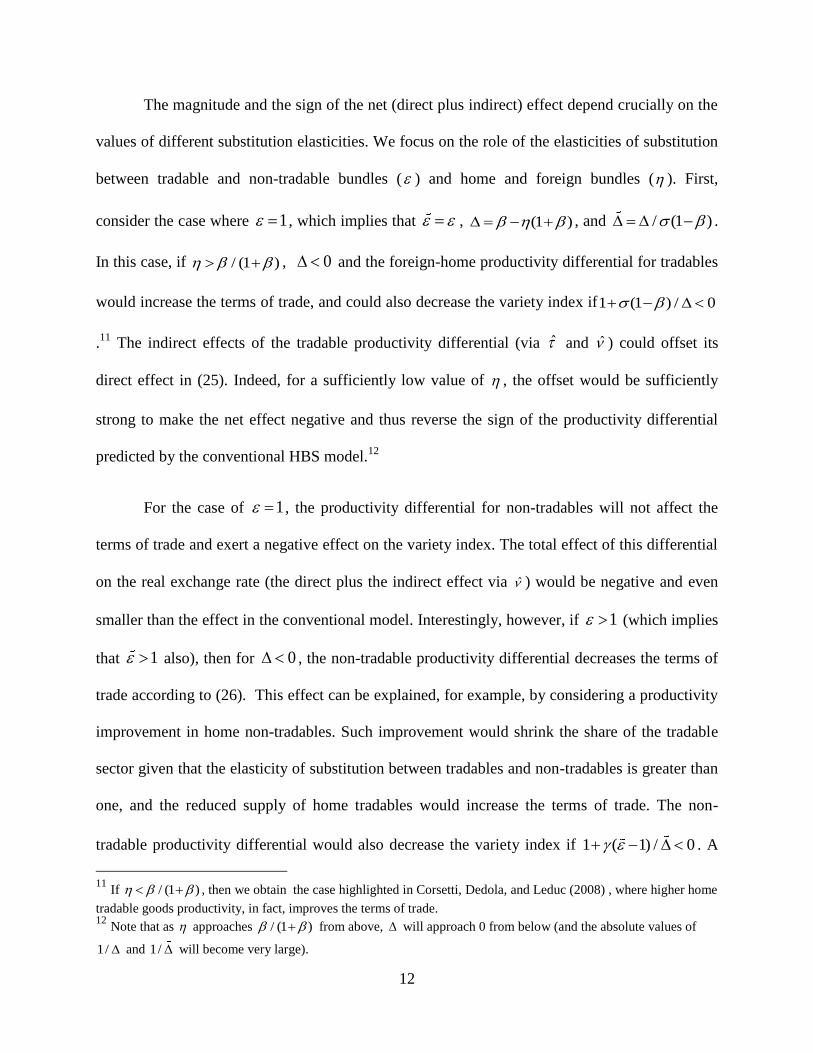
The magnitude and the sign of the net (direct plus indirect) effect depend crucially on the

values of different substitution elasticities. We focus on the role of the elasticities of substitution

between tradable and non-tradable bundles ( ) and home and foreign bundles ( ). First,

consider the case where 1 , which implies that , (1 ) , and / (1 ) .

In this case, if / (1 ) , 0 and the foreign-home productivity differential for tradables

would increase the terms of trade, and could also decrease the variety index if1 (1 ) / 0

.11

The indirect effects of the tradable productivity differential (via ̂ and ̂ ) could offset its

direct effect in (25). Indeed, for a sufficiently low value of , the offset would be sufficiently

strong to make the net effect negative and thus reverse the sign of the productivity differential

predicted by the conventional HBS model.12

For the case of 1 , the productivity differential for non-tradables will not affect the

terms of trade and exert a negative effect on the variety index. The total effect of this differential

on the real exchange rate (the direct plus the indirect effect via ̂ ) would be negative and even

smaller than the effect in the conventional model. Interestingly, however, if 1 (which implies

that 1 also), then for 0 , the non-tradable productivity differential decreases the terms of

trade according to (26). This effect can be explained, for example, by considering a productivity

improvement in home non-tradables. Such improvement would shrink the share of the tradable

sector given that the elasticity of substitution between tradables and non-tradables is greater than

one, and the reduced supply of home tradables would increase the terms of trade. The non-

tradable productivity differential would also decrease the variety index if 1 ( 1) / 0 . A

11

If / (1 ) , then we obtain the case highlighted in Corsetti, Dedola, and Leduc (2008) , where higher home

tradable goods productivity, in fact, improves the terms of trade. 12

Note that as approaches / (1 ) from above, will approach 0 from below (and the absolute values of

1/ and 1/ will become very large).

13

larger would enhance the effect of the differential on both the terms of trade and the variety

index. The indirect effects through these channels could be large enough for a sufficiently large

value of to more than offset the direct effect, and thus also reverse the sign of the coefficient

of non-tradable productivity differential in the conventional model.

The model can also be solved for income per capita. As the Appendix shows, the income

per capita in each country depends on productivity levels and the number of varieties in the two

sectors as well as the terms of trade. Solving for the number of varieties and the terms of trade,

the income differential can be expressed as:

* * *( 1) (1 ) 1ˆ ˆ ˆ ˆˆ ˆ 1 ( ) 1 ( )( 1) ( 1) (1 )

N N F Hy y A A A A

(28)

The effects of the two productivity differentials on the income differential now depend on the

various elasticities of substitution.

2.4 Empirical Implementation

In empirically implementing the two-country model to a multi-country set ( S ) of OECD

countries, we let the home country represent an OECD country (indexed by c S ) and the

foreign country stand for the rest of the world (indexed by W ). In view of (15) and (25-27), we

specify our empirical relations as

0 1 , , 2 , ,ln (ln ln ) (ln ln )cWt c c T Wt T ct c N Wt N ct ctQ A A A A u (29)

where for period t , cWtQ represents country c ’s real effective exchange rate (relative to the

rest of the world); , , and T ct T WtA A denote the productivity levels for tradable sectors in country c

14

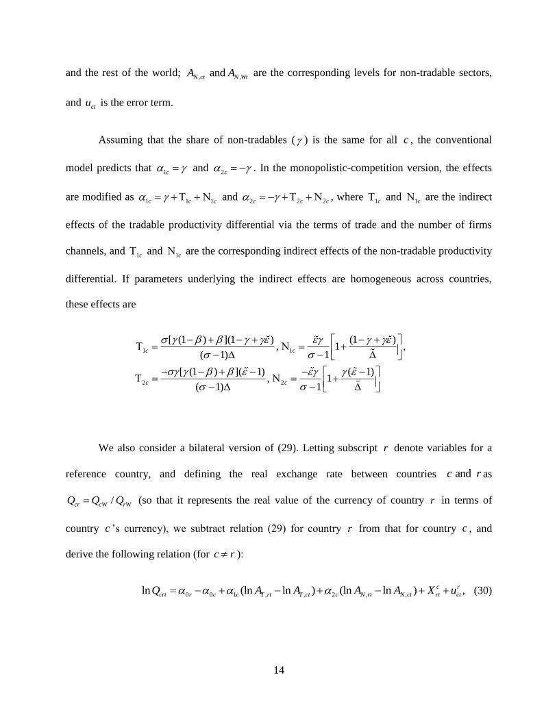
and the rest of the world; , , and N ct N WtA A are the corresponding levels for non-tradable sectors,

and ctu is the error term.

Assuming that the share of non-tradables ( ) is the same for all c , the conventional

model predicts that 1c and 2c . In the monopolistic-competition version, the effects

are modified as 1 1 1c c c and 2 2 2c c c , where 1c and 1c are the indirect

effects of the tradable productivity differential via the terms of trade and the number of firms

channels, and 1c and 1c are the corresponding indirect effects of the non-tradable productivity

differential. If parameters underlying the indirect effects are homogeneous across countries,

these effects are

1 1

2 2

[ (1 ) ](1 ) (1 ) , 1 ,

( 1) 1

[ (1 ) ]( 1) ( 1), 1

( 1) 1

c c

c c

We also consider a bilateral version of (29). Letting subscript r denote variables for a

reference country, and defining the real exchange rate between countries and c r as

/cr cW rWQ Q Q (so that it represents the real value of the currency of country r in terms of

country c ’s currency), we subtract relation (29) for country r from that for country c , and

derive the following relation (for c r ):

0 0 1 , , 2 , ,ln (ln ln ) (ln ln ) ,c r

crt r c c T rt T ct c N rt N ct rt ctQ A A A A X u (30)

15

where 1 1 , , 2 2 , ,( )(ln ln ) ( )(ln ln )c

rt c r T Wt T rt c r N Wt N rtX A A A A , and r

ct ct rtu u u . If

coefficients of productivity differentials are homogeneous, then 1 1c r and 2 2c r , and

0c

rtX . In the absence of homogeneity, 0r

ctX and the omission of this variable would

introduce cross-sectional dependence in the panel data.

3. Empirical Results

3.1 Data

For the empirical analysis we collect annual data from 1977 to 2006 for 16 OECD

countries: Austria, Belgium, Canada, Denmark, Finland, France, Germany, Italy, Japan, Korea,

the Netherlands, Norway, Portugal, Sweden, the United Kingdom and the United States. The

choice of the countries in our panel is determined by the availability of a comparable set of the

variables of interest for a sufficiently long time span.

We obtain data for the bilateral nominal exchange rates, measured in local currency per

US dollar, and the consumer price index from the International Financial Statistics of the IMF.13

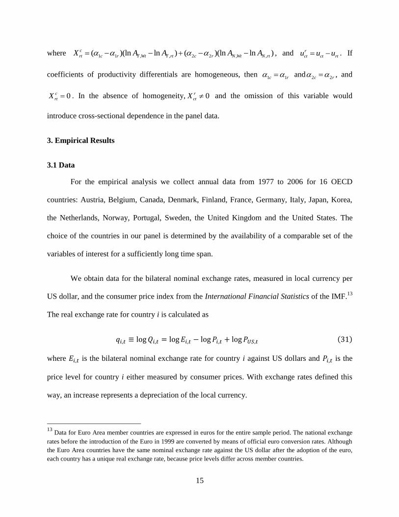
The real exchange rate for country i is calculated as

where is the bilateral nominal exchange rate for country i against US dollars and is the

price level for country i either measured by consumer prices. With exchange rates defined this

way, an increase represents a depreciation of the local currency.

13

Data for Euro Area member countries are expressed in euros for the entire sample period. The national exchange

rates before the introduction of the Euro in 1999 are converted by means of official euro conversion rates. Although

the Euro Area countries have the same nominal exchange rate against the US dollar after the adoption of the euro,

each country has a unique real exchange rate, because price levels differ across member countries.

16

Labor productivity is measured as value added volume per employee. We obtain the

series for value added volume and number of persons engaged (total employment) from the

Structural Analysis Industrial Database (STAN) provided by the Organization for Economic Co-

operation and Development (OECD) for 9 industries: agriculture, hunting, forestry and fishing;

mining and quarrying; manufacturing; transport, storage and communications; electricity, gas

and water supply; construction; wholesale and retail trade, restaurants and hotels; finance,

insurance, real estate and business services; and community, social, and personal services.

Following De Gregorio et al. (1994) who use export shares in total production as a measure for

tradability, we classify the first four industries as the tradable sector and the other five as the

non-tradable sector.14

Log labor productivities for the tradable and non-tradable sectors of

country i are computed as follows:

radables , on tradables

where is value-added volume and is total employment for country i in sector s at

time t. This is equivalent to taking the weighted average of labor productivity of the individual

industries in the tradable and non-tradable sectors, with employment shares as weights.15

We

14

The classification of sectors into tradable and non-tradable goods is somewhat arbitrary and might change over

time, in particular, given the greater role of services in the tradable sector (see MacDonald and Ricci, 2001).

15 The productivity dataset for Sweden is not complete. Value added volume and total employment for wholesale

and retail trade, restaurants and hotels, a non-tradable sector, are missing from 1977 to 1992; value added volume

for transport, storage and communications, a tradable sector, is missing from 1977 to 1992. We assume that the

missing series grew at the average rate of the other industries in the same sector over the missing period. Therefore, we can construct the value added volume for transport, storage and communications for 1992 by applying the

weighted average growth rate of the value added volume of the other three industries in the tradable sector to the

available observation for 1993. We construct the whole missing period by repeating this process backward in time.

The two missing series for wholesale and retail trade, restaurants and hotels are constructed in the same way. Mining

and quarrying data for Portugal are missing for entire sample. We could not construct the missing series with the

above method, because we do not have a single available observation to which the average growth rate can be

applied. Therefore, we omit mining and quarrying entirely. This treatment is equivalent to assuming that the labor

productivity in mining and quarrying is same as the average labor productivity in the other tradable industries

weighted by their employment share.

17

also construct an economy-wide labor productivity measure by aggregating the tradable and non-

tradable sectors in the same way.

In the estimations, we use labor productivity differentials, which are the differences

between the log labor productivity of a reference country R and each country i for the tradable

and non-tradable sectors, defined as ( and ( ) respectively. Given

that it is a well-known fact that estimation results might be sensitive to the choice of the

numéraire currency,16

we consider three different reference countries: the United States,

Germany and “the rest of the world” (as defined by our set of OECD countries). Following

Chong et al. (2010), the set of world-based variables is constructed by subtracting the average

over all the countries in the panel from the series relative to the United States. More specifically,

we compute

, where

corresponds to the U.S.-based variable

and N equals the number of countries. This transformation is essentially equivalent to cross-

sectional demeaning. In what follows, the latter set of variables serves as the benchmark dataset,

whereas results obtained with the United States and Germany as the base countries are reported

in the Appendix.

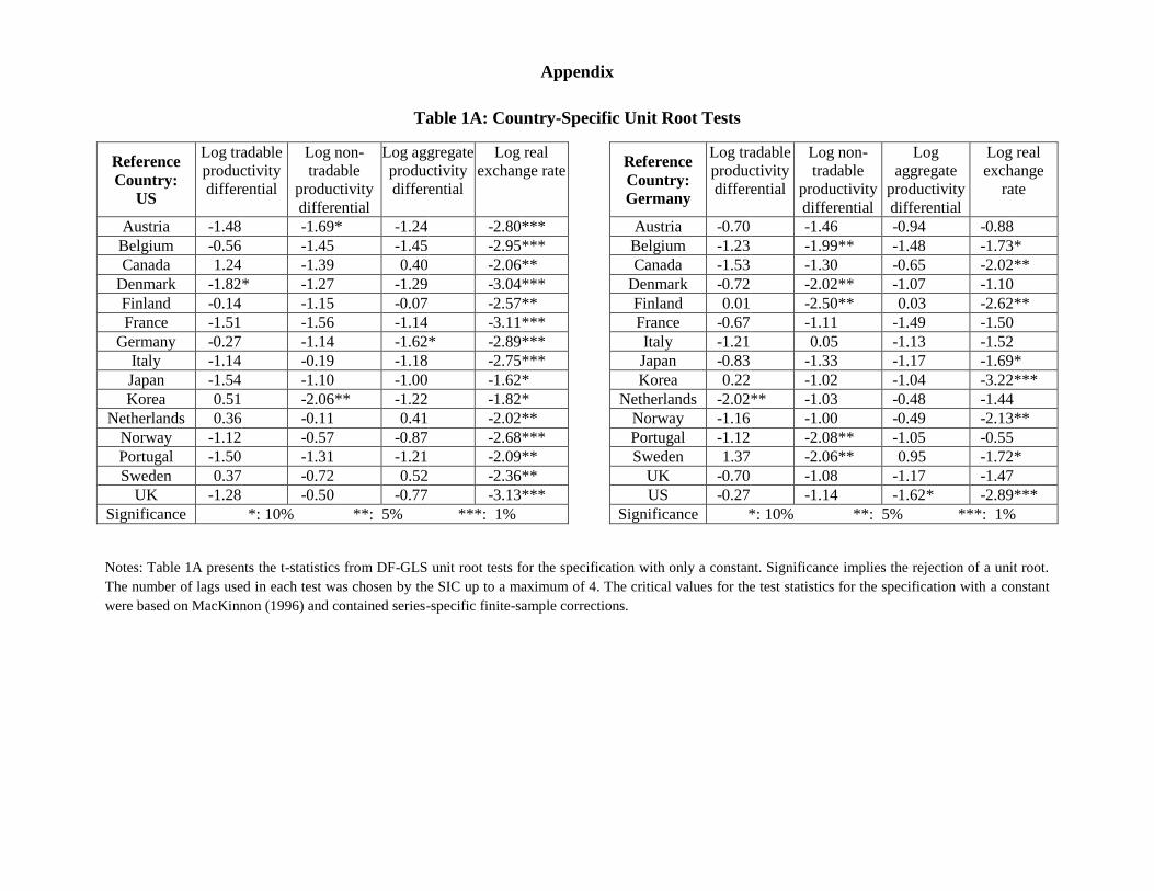
3.2 Unit-Root Tests

Given that our interest centers on modeling the long-run relationship between real

exchange rates and the productivity differentials in the tradable and non-tradable sectors, we first

have to establish whether the variables in our dataset follow unit-root processes. Table 1, panel

A, reports univariate unit-root tests for each of the variables in our panel for individual countries

based on the DF-GLS procedure proposed by Elliott, Rothemberg, and Stock (1996). While the

16

For example, Canzoneri, Cumby, and Diba (1999) show that tests of the HBS hypothesis turn out much more

favorably when Germany rather than the US is chosen as the reference country. Sources of potential bias are cross-

sectional correlation in the error term and idiosyncratic developments in the base country.

18

evidence of non-stationarity is relatively uniform across countries for the three productivity

measures with only a few exceptions, the results for the real exchange rates are more mixed.17

However, the unit-root tests based on individual time series are inconclusive since they

tend to have low power in short samples. Jointly exploiting the information contained in the

time-series and cross-sectional dimension of the data, should increase the power of these tests.

For this reason, we employ a number of unit-root tests using panel-data techniques proposed by

Im, Pesaran, and Shin (2003), Choi (2001), and Maddala and Wu (1999).

Table 1, panel B, summarizes the results from these panel unit-root tests for the world-

based series. Using this more powerful panel approach, we cannot reject the null hypothesis that

all the productivity measures in the panel contain a unit root according to all three tests.

Nonetheless, the evidence for non-stationarity remains weak in the case of the real exchange

rate.18

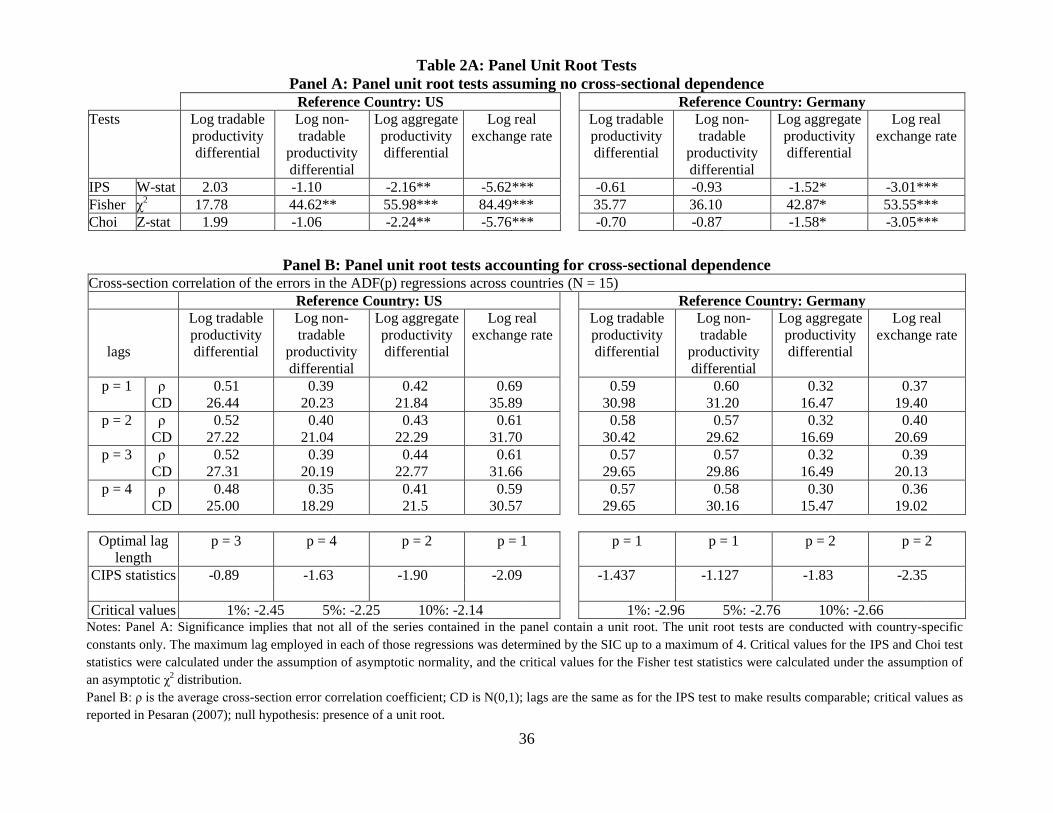
While these panel-based tests allow for heterogeneity in coefficients, one potential

drawback is that, for the tests to be valid, the underlying individual series must be independent of

each other. This requirement might not be satisfied in our sample because of common factors

determining real exchange rates. To ascertain the validity of this assumption, we conduct tests on

the cross-sectional dependence of the error terms suggested by Pesaran (2004).

According to this test, the cross-sectional demeaning that is implicit in the construction of

the world-based series was sufficient to remove dependence among panel members.19

However,

as can be seen from Table 2A, panel B, the cross-section dependence (CD) test statistics is highly

significant for all US-based and Germany-based series, indicating strong correlation of the error

17

The strongest rejection for the presence of a unit root in the real exchange rate is found for the US-based series as

can be seen in Table 1A. 18

Chong et al. (2010) obtain a similar finding. 19

The average cross-equation error correlation coefficients for all world-based series range between 0.01 and 0.06,

indicating that cross-sectional dependence is not an issue.

19

terms across the units in the panel for both specifications. Therefore, we employ the modified

IPS test (CIPS) introduced by Pesaran (2007) that corrects for cross-sectional dependence. This

test provides evidence for the presence of a unit root in all of the series in our dataset.

3.3 Panel Cointegration Tests

To analyze the long-run effects of productivity differentials on the real exchange rate, we

investigate whether there exists a cointegration relationship between the real exchange rate and

productivity differentials in the tradable and non-tradable sectors. We conduct the same analysis

for the specification where only the aggregate productivity measure (that is, real income per

worker) is considered.

The null hypothesis of no cointegration is tested using three residual-based tests

suggested by Pedroni (1999, 2004) which do not impose homogeneity of the cointegrating vector

i.e. the test allows for potentially heterogeneous slope parameters for each country. These tests

rely on the group-mean statistics, that is, the unit root tests on the estimated residuals derived

from the following equation are pooled along the between-dimension of the panel20

:

Table 2 shows that the evidence for cointegration is mixed for both specifications obtained with

the world-based series. This result carries over to the specifications in which the U.S. and

Germany are chosen as the reference country as emerges from Table 3A.

However, the critical values used to judge the significance of the test statistics are derived

under the assumption of cross-sectional independence in the error term across countries which is

not necessarily the case as shown above. In addition, the Pedroni (2007) tests, as most residual-

based cointegration tests, require the common-factor restriction to be satisfied. That is, the long-

20

For the specification with the aggregate productivity measure, the number of regressors in equation (33) is

reduced by one.

20

run parameters of the variables in levels are constrained to be equal to the short-run parameters

of the variables in first difference. The violation of this assumption can significantly reduce the

power of those tests.

Therefore, we also carry out the set of cointegration tests suggested by the Westerlund

(2007), which explicitly allow the short-run dynamics to differ from the long-run cointegrating

relationships in obtaining the residuals on which the tests are performed and take cross-sectional

correlation into account. Table 2 shows that all four Westerlund (2007) test statistics find strong

evidence for panel cointegration among the world-based series.21

This result is confirmed for the

U.S.-based and Germany-based specifications (see Table 3A).

3.4 Estimation of Long-Run Effects

Based on the evidence in support of the existence of a long-run relationship between the

real exchange rate and the labour productivity differentials in the tradable and non-tradable

sectors, we estimate the cointegrating vector based on the following empirical model:

where δi captures country-specific effects, with , are the long-run cointegrating

coefficients, with , are the coefficients of leads and lags of the first differences

of the productivity differentials that control for endogeneity and is the residual term.22

21

These tests were carried out in STATA with code prepared by Persyn and Westerlund (2008). Robust critical

values were generated by 800 times bootstraps. 22

We only include one lead and one lag in order not to lose too many degrees of freedom given that our sample is

relatively short.

21

Following Lee and Tang (2007) amongst others, we employ a panel DOLS estimator that

pools information along the within-dimension (see Kao and Chiang 1997) to estimate the long-

run effects of productivity differentials in the tradable and non-tradable sectors on the real

exchange rate. This technique implies that restricting both the long-run coefficients and the

transitional dynamics to be the same across countries, i.e. , ,

and , for all i=1,2,...N. Hence, only the constant is allowed to differ thereby

accounting for time-invariant country-specific factors which should help reduce omitted-variable

bias. Results are reported in Table 3. Contrary to the HBS hypothesis, we find a statistically

significant negative effect of the productivity differential in the tradable sector on real exchange

rates, while the effect of the non-tradable sector is of similar magnitude and of opposite sign but

not statistically significant. The effect of the aggregate (per worker) productivity differential is

also negative but insignificant.

The presence of important differences in the short-run adjustment process across

countries may, however, restrict the applicability of the fixed-effect panel DOLS estimator. For

this reason, we use the pooled mean-group estimator for heterogeneous panels proposed by

Pesaran, Shin, and Smith (1999) which allows short-run coefficients and error variances to be

different across panel members but imposes the same cointegrating vector for all cross sections

i.e. pools the information regarding the long-run relationship. Table 4 presents the estimates of

the long-run coefficients obtained with this hybrid model. Again we find a highly statistically

significant negative coefficient on the productivity differential in the tradable sector as well as on

the aggregate productivity measure implying that an increase in tradable goods and total

productivity in the home country tends to depreciate the real exchange rate. Productivity

22

differentials in the non-tradable sector are not statistically significant determinants of the real

exchange rate.

Homogeneity misspecification can also arise from constraining the long-run equilibrium

relationship to be identical across countries. To also allow for the possibility of heterogeneous

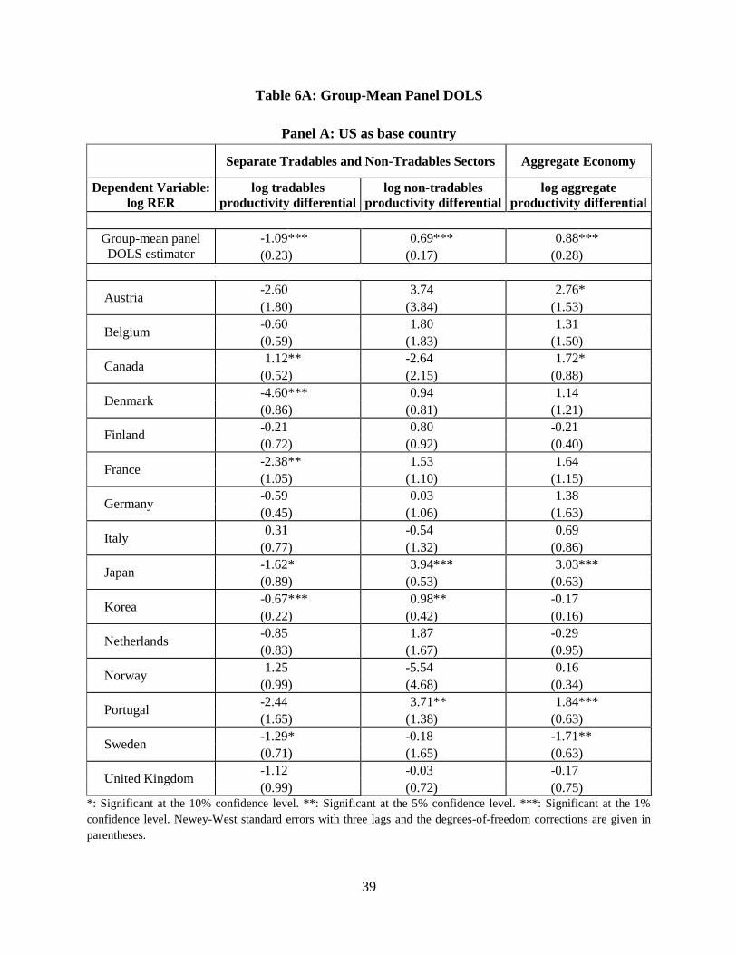
cointegrating relationships, we employ the between-dimension estimator proposed by Pedroni

(2001). This entails estimating equation (34) separately for each country and then using these

coefficient estimates to construct the group mean panel DOLS estimator in the following way:

where , . More specifically, the group-mean panel DOLS

estimator is derived by pooling information along the between-dimension and hence can be

interpreted as an average value (over the panel members) in the presence of heterogeneity. In this

way, we are not only able to obtain a summary measure of the long-run productivity effects, but

to study potential cross-country differences of such effects. Table 5 contains the results for the

group-mean panel DOLS estimator, and , as well as the estimated individual

slopes, and for all i=1,2,...N for the tradable and non-tradable sectors respectively. The

last column of Table 5 reports the corresponding estimates for the economy-wide productivity

differential. While the average values of the long-run coefficients is broadly in line with results

obtained with the other two estimation methods, we find substantial heterogeneity in the cross-

sectional dimension. Estimates of the cointegrating vector vary greatly across countries without,

however, displaying a clear pattern that would help explain the size and direction of the

estimated effects.

4. Reconciling the Evidence

Our results for individual countries indicate (Table 5) considerable heterogeneity of

coefficients across countries. Estimation of average effects by three different procedures (Tables

23

3-5) shows that the coefficient of the tradable productivity differential is negative and significant

in all cases, while the coefficient of the non-tradable productivity differential is positive but

significant only in one case (Group-Mean Panel DOLS). The signs and the magnitudes of these

coefficients are clearly inconsistent with the conventional HBS model. The conventional model,

moreover, does not account for coefficient heterogeneity across countries.

This section examines whether the above results can be reconciled with the monopolistic-

competition version of the HBS model. To explore this question, we simulate the quantitative

version of the HBS model discussed in Section 2.2 using different values of the key underlying

elasticities. To calibrate our model to OECD countries, we set equal to the median share of

non-tradables, and equal to the median difference between the shares of domestic and

imported goods in tradables.23

These values are 0.73 for and 0.3 for .24

For the elasticity of

substitution for goods with each (tradable/non-tradable) aggregate, we set = 6. This value

implies a demand markup [ / ( 1) ] equal to 0.2, which is consistent with estimates for OECD

countries (Martins, Scarpetta, and Pilat, 1996).

There is considerable controversy about the value of the elasticity of substitution between

home and foreign tradable goods, . Estimates based on fitting aggregate data to macro models

indicate that the value of this elasticity is low and below 1.0 (Bergin, 2006; Lubik and

Schorfheide, 2005). Studies based on the disaggregated trade data, on the other hand, suggest the

average value of the elasticity to be much larger (Imbs and Mejean, 2009). The larger values,

however, are based on estimates of the elasticities of substitution between imports from different

23

Note that home bias is defined as * , where and * represent the shares of home goods in home and

foreign bundles of tradables. Assuming homogeneity, * is measured by the share of imports in tradables.

24 Average values for our sample period, 1977-2006, are used to calculate the shares for each country.

24

countries (that is, trade elasticities). Trade elasticities can be used as a measure of under the

assumption that the elasticity of substitution between any two varieties is the same regardless of

the country where they are produced. This assumption need not hold and home and foreign

goods could be less substitutable than imports from different countries. In this case, the value of

would be smaller than (the average value of) trade elasticities.25

Estimation of the elasticity of substitution between tradable and non-tradable goods, ,

has received less attention. In macro models this elasticity is typically assumed to be close to

one. But this assumption is not based on empirical estimation, and it is not implausible that this

elasticity could be greater than one.

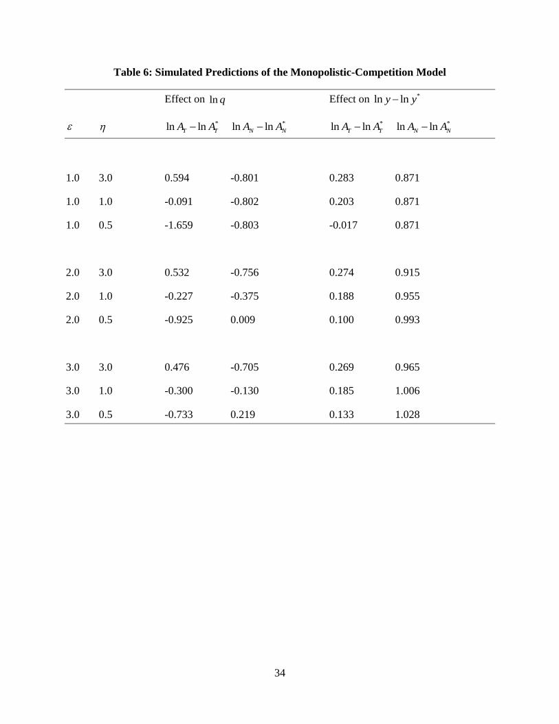
In view of the uncertainty about the values of and , we consider a wide range of

values of these elasticities to derive the predictions of our quantitative model for the effects of

the tradable and non-tradable productivity differentials. Table 6 shows the elasticity of the real

exchange rate and the per capita productivity differential with respect to tradable and non-

tradable productivity differentials for selected values of and . First, we consider the

conventional assumption that is close to unity (so that the consumption index is approximated

by the Cobb-Douglas form) so that the expenditure shares between tradable and non-tradable

goods remain constant when relative prices change. In this case, if 3 (a value much larger

than the macro-level estimates), then as in the conventional HBS model, the effect on the real

exchange rate of the log productivity differential for tradables is positive and large while that for

non-tradables is negative and large. Indeed, the absolute value of the effects of the two

differentials is larger than the share of non-tradables (as in conventional HBS model). However,

25

Imbs and Mejean (2009) argue, however, that the macro-level estimates of are too low because of aggregation

bias due to heterogeneity of substitution elasticities across products.

25

for smaller values of (values close to the range of macro-level estimates), the elasticity of the

real exchange rate with respect to the tradable differential falls sharply and its sign is reversed.

For example, this elasticity is negative for 1 , and below -1.5 for 0.5 . The intuition

behind these results is that for low values of an increase in tradable goods productivity will

cause a significant decline in the terms of trade and a depreciation of the real exchange rate.

Consequently, these cases can explain our result of the estimated negative coefficient on tradable

differential, but not the estimated positive coefficient on the non-tradable differential. The

elasticity of the real exchange rate with respect to the non-tradable differential is negative and

below as long as 1 .

The effects of the productivity differentials change significantly for values of 1 . As

increases (above one), the effect of the non-tradable productivity differential increases, while the

tradable differential effect decreases. Large values of combined with small values of can

lead to positive values of the effect of non-tradable differential. For example, with 0.5 , a

value of equal to 2 is sufficient to raise the non-tradable differential effect to above zero and a

value of 3 would further raise it to 0.2. With a large value of , increases in nontradable

goods productivity will reduce their relative price causing a sizable shift in demand towards

these goods; consequently to supply these goods would require a reduction in the supply of

tradable goods, which would increase the terms of trade and appreciate the real exchange rate.

These values for the two elasticities also imply a large negative effect of the tradable differential,

and thus would be broadly consistent with our estimates.

The above results about the values of elasticities needed to reconcile the evidence are

based on a simple monopolistic-competition model. In our future work, we plan to explore the

26

robustness of our results in richer models. One possibility is to consider extensions that would

allow the price elasticity of demand for domestic tradable goods and imports to differ from the

elasticity of substitution between these goods. Another and a more major extension would be to

allow for heterogeneous productivity across firms which would introduce additional channels,

including through changes in the extensive margin, for the transmission of productivity changes

to the real exchange rate.

Other challenges are to explain the heterogeneous coefficient estimates across countries

and sensitivity of the results to the choice of the reference country and the set of countries

included in the analysis.26

Heterogeneity could arise because of international differences in key

parameters such as the elasticities of substitution between home and foreign tradable goods and

between tradable and non-tradable goods. The magnitude of cross-country parameter variation

needed to explain the heterogeneity of estimated coefficients, however, appears to be too large.

An alternative explanation of heterogeneity is that the estimates are obtained from time series

that are not long enough for low-frequency estimates to converge to long-run (steady-state)

values. Consequently, the limited length of our sample period results in very imprecise estimates

for the separate real exchange rate equations for each country.

To explore the robustness of our results further, we re-estimated the regression model

given by (34) to obtain the group mean DOLS estimates of the coefficients on the tradable and

nontradables productivity differentials using different sample periods. The plots of the

coefficients for the world-based and U.S.-based estimates are given in Charts 1a and 1b. An

important finding is that the signs of the estimated coefficients are sensitive to the sample period

26

We refer the reader to Tables 4A-6A in the Appendix for the results obtained with U.S. and Germany as the

reference countries. However, we do not include the estimates obtained for various subsets of countries.

27

as well as to the basis (world versus U.S.) used for comparison. The most striking finding is that

with the U.S. based series, the signs of the estimated coefficients for samples ending prior to

1998 are consistent with the HBS hypothesis, but that the signs reverse after 1998 and are

consistent with our findings for the full sample. Interestingly, Lee and Tang (2007) use a sample

that ends in 1997 and obtain HBS-consistent coefficient estimates. The rationale for the reversal

in the signs of the estimated coefficients after 1997 is not obvious; it could reflect the formation

of the Euro Area or the emergence of China, which caused profound changes in the world

relative prices of traded manufactured goods and commodities as well as contributing to

persistent global imbalances.

As pointed out by Lee and Tang (2007), for OECD countries with similar levels of

productivity, the dynamics of the real exchange rate are also determined by other factors

including cyclical macroeconomic forces, including trade and current account imbalances, and

relative commodity price movements that might mask the long-term productivity effects. This

implies that if fundamentals other than productivity growth play an important role for the long-

run behaviour of real exchange rates, then omitting these factors could bias the results.

5. Future work

To better understand our empirical results, we plan to investigate further the robustness of our

results and explain observed differences. We would also like to consider a dynamic version of

the model which would include nominal rigidities and additional shocks. We would use such a

model to investigate the variability of low-frequency estimates based on simulations over a

period comparable to the length of our sample, and examine if it is large enough to explain the

observed heterogeneity

28

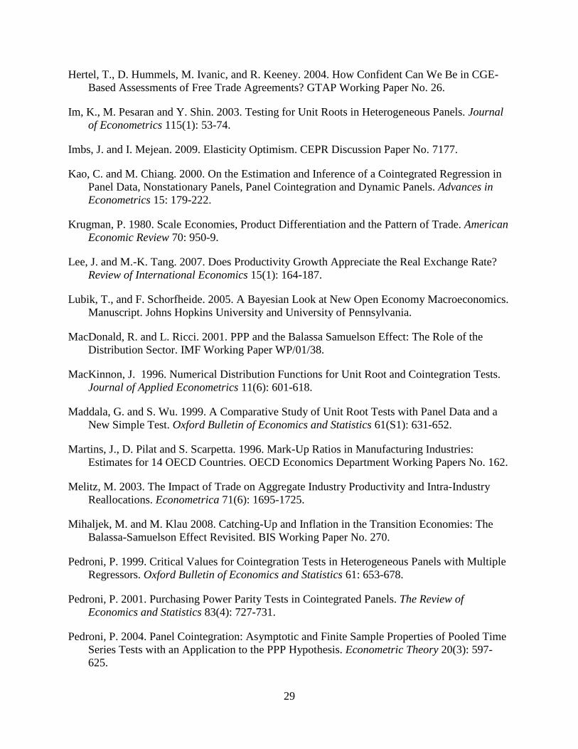
References

Balassa, B. 1964. The Purchasing Power Parity Doctrine: A Reappraisal. Journal of Political

Economy, 72: 584–96.

Benigno, G. and C. Thoenissen. 2003. Equilibrium Exchange Rates and Supply-Side

Performance. Economic Journal 113: 103-24.

Bergin, P. 2006. How Well Can the New Open Economy Macroeconomics Explain the

Exchange Rate and Current Account? Manuscript. University of California at Davis.

Canzoneri, M., R. Cumby and B. Diba. 1999. Relative Labor Productivity and the Real

Exchange Rate in the Long Run: Evidence for a Panel of OECD Countries. Journal of

International Economics 47(2): 245-266.

Chinn, M. and L. Johnson. 1999. The Impact of Productivity Differentials on Real Exchange

Rates: Beyond the Balassa Samuelson Framework. Manuscript. University of California

Santa Cruz.

Choi, I. 2001. Unit root tests for panel data. Journal of International Money and Finance 20(2):

249-272.

Chong, Y., O. Jordà and A. Taylor. 2010. The Harrod-Balassa-Samuelson Hypothesis: Real

Exchange Rates and Their Long-Run Equilibrium. International Economic Review.

forthcoming.

Choudhri, E. and L. Schembri. 2010. Productivity, the Terms of Trade and the Real Exchange

Rate: The Balassa-Samuelson Hypothesis Revisited. Review of International Economics,

forthcoming.

Corsetti, G., L. Dedola and S. Leduc. 2008. International Risk Sharing and the Transmission of

Productivity Shocks. Review of Economic Studies 75: 443-473.

De Gregorio, J., A. Giovannini and H. Wolf. 1994. International Evidence on Tradables and

Nontradables Inflation. European Economic Review. 38(6): 1225-1244.

Elliott, G., T. Rothenberg and J. Stock. 1996. Efficient Tests for an Autoregressive Unit Root.

Econometrica 64(4): 813-836.

Freeman, R. 2008. Labour Productivity Indicators: Comparison of Two OECD Databases

Productivity Differentials and the Balassa Samuelson Effect. Paris: OECD.

Ghironi, F., and M. Melitz. 2005. International Trade and Macroeconomic Dynamics with

Heterogeneous Firms. Quarterly Journal of Economics 120: 865-915.

Harrod, R. 1933. International Economics. London: Nisbet and Cambridge University Press.

Harrod, R.F. 1939. An Essay in Dynamic Theory. The Economic Journal 49: 14-33.

29

Hertel, T., D. Hummels, M. Ivanic, and R. Keeney. 2004. How Confident Can We Be in CGE-

Based Assessments of Free Trade Agreements? GTAP Working Paper No. 26.

Im, K., M. Pesaran and Y. Shin. 2003. Testing for Unit Roots in Heterogeneous Panels. Journal

of Econometrics 115(1): 53-74.

Imbs, J. and I. Mejean. 2009. Elasticity Optimism. CEPR Discussion Paper No. 7177.

Kao, C. and M. Chiang. 2000. On the Estimation and Inference of a Cointegrated Regression in

Panel Data, Nonstationary Panels, Panel Cointegration and Dynamic Panels. Advances in

Econometrics 15: 179-222.

Krugman, P. 1980. Scale Economies, Product Differentiation and the Pattern of Trade. American

Economic Review 70: 950-9.

Lee, J. and M.-K. Tang. 2007. Does Productivity Growth Appreciate the Real Exchange Rate?

Review of International Economics 15(1): 164-187.

Lubik, T., and F. Schorfheide. 2005. A Bayesian Look at New Open Economy Macroeconomics.

Manuscript. Johns Hopkins University and University of Pennsylvania.

MacDonald, R. and L. Ricci. 2001. PPP and the Balassa Samuelson Effect: The Role of the

Distribution Sector. IMF Working Paper WP/01/38.

MacKinnon, J. 1996. Numerical Distribution Functions for Unit Root and Cointegration Tests.

Journal of Applied Econometrics 11(6): 601-618.

Maddala, G. and S. Wu. 1999. A Comparative Study of Unit Root Tests with Panel Data and a

New Simple Test. Oxford Bulletin of Economics and Statistics 61(S1): 631-652.

Martins, J., D. Pilat and S. Scarpetta. 1996. Mark-Up Ratios in Manufacturing Industries:

Estimates for 14 OECD Countries. OECD Economics Department Working Papers No. 162.

Melitz, M. 2003. The Impact of Trade on Aggregate Industry Productivity and Intra-Industry

Reallocations. Econometrica 71(6): 1695-1725.

Mihaljek, M. and M. Klau 2008. Catching-Up and Inflation in the Transition Economies: The

Balassa-Samuelson Effect Revisited. BIS Working Paper No. 270.

Pedroni, P. 1999. Critical Values for Cointegration Tests in Heterogeneous Panels with Multiple

Regressors. Oxford Bulletin of Economics and Statistics 61: 653-678.

Pedroni, P. 2001. Purchasing Power Parity Tests in Cointegrated Panels. The Review of

Economics and Statistics 83(4): 727-731.

Pedroni, P. 2004. Panel Cointegration: Asymptotic and Finite Sample Properties of Pooled Time

Series Tests with an Application to the PPP Hypothesis. Econometric Theory 20(3): 597-

625.

30

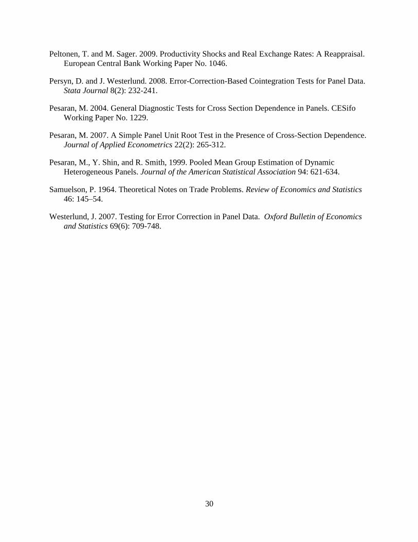
Peltonen, T. and M. Sager. 2009. Productivity Shocks and Real Exchange Rates: A Reappraisal.

European Central Bank Working Paper No. 1046.

Persyn, D. and J. Westerlund. 2008. Error-Correction-Based Cointegration Tests for Panel Data.

Stata Journal 8(2): 232-241.

Pesaran, M. 2004. General Diagnostic Tests for Cross Section Dependence in Panels. CESifo

Working Paper No. 1229.

Pesaran, M. 2007. A Simple Panel Unit Root Test in the Presence of Cross-Section Dependence.

Journal of Applied Econometrics 22(2): 265-312.

Pesaran, M., Y. Shin, and R. Smith, 1999. Pooled Mean Group Estimation of Dynamic

Heterogeneous Panels. Journal of the American Statistical Association 94: 621-634.

Samuelson, P. 1964. Theoretical Notes on Trade Problems. Review of Economics and Statistics

46: 145–54.

Westerlund, J. 2007. Testing for Error Correction in Panel Data. Oxford Bulletin of Economics

and Statistics 69(6): 709-748.

31

Table 1: Unit Root Tests

Panel A: Country-Specific Unit Root Tests

Log tradable

productivity differential

Log non-tradable


Log aggregate


Log real exchange rate

Austria -0.75 -1.27 -1.04 -1.82 *

Belgium 0.03 -2.00 ** 0.20 -2.44 **

Canada 0.47 -0.98 -0.28 -2.55 **

Denmark -1.00 -1.91 * -0.35 -1.81 *

Finland 1.18 -1.40 0.49 -0.92

France -1.63 * -0.26 -0.01 -2.41 **

Germany -0.43 -2.77 *** -0.65 -2.20 **

Italy -0.85 0.04 0.34 -1.92 *

Japan -1.16 -1.48 -1.95 * -1.61 *

Korea 0.31 -0.83 0.13 -3.00 ***

Netherlands -0.42 -0.61 -0.26 -2.36 **

Norway -1.08 -0.85 -1.00 -2.17 **

Portugal -1.46 -1.91 * -1.55 -0.36

Sweden -0.31 -1.05 -0.82 -0.88

United Kingdom -0.68 0.07 -2.42 ** -1.30

Significance *: 10% **: 5% ***: 1%

Panel B: Panel Unit Root Tests Tests Log tradable


Log non-tradable


Log aggregate


Log real exchange rate

IPS W-stat 2.40 0.44 1.06 -2.81 ***

Fisher χ2

17.06 31.15 37.11 53.39 ***

Choi Z-stat 2.34 0.32 0.85 -2.86 ***

Notes: Panel A presents the t-statistics from DF-GLS unit root tests for the specification with only a constant. Significance implies the rejection of a unit root.

The number of lags used in each test was chosen by the SIC up to a maximum of 4. The critical values for the test statistics for the specification with a constant

were based on MacKinnon (1996) and contained series-specific finite-sample corrections.

Panel B: Significance implies that not all of the series included in the panel contain a unit root. The unit root tests are conducted with country-specific constants

only. The maximum lag employed in each of those regressions was determined by the SIC up to a maximum of 4. Critical values for the IPS and Choi test

statistics were calculated under the assumption of asymptotic normality, and the critical values for the Fisher test statistics were calculated under the assumption

of an asymptotic χ2 distribution.

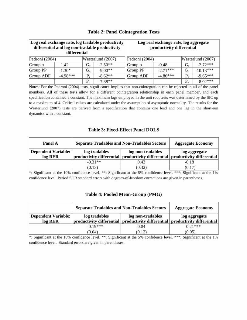
Table 2: Panel Cointegration Tests

Log real exchange rate, log tradable productivity

differential and log non-tradable productivity

differential

Log real exchange rate, log aggregate


Pedroni (2004) Westerlund (2007) Pedroni (2004) Westerlund (2007)

Group ρ 1.42 Gτ -2.50 ** Group ρ -0.48 Gτ -2.72 ***

Group PP -1.30 * Gα -9.00 ** Group PP -2.71 *** Gα -10.13 ***

Group ADF -4.98 *** Pτ -8.62 ** Group ADF -4.86 *** Pτ -9.65 ***

Pα -7.38 ** Pα -8.02 ***

Notes: For the Pedroni (2004) tests, significance implies that non-cointegration can be rejected in all of the panel

members. All of these tests allow for a different cointegration relationship in each panel member, and each

specification contained a constant. The maximum lags employed in the unit root tests was determined by the SIC up

to a maximum of 4. Critical values are calculated under the assumption of asymptotic normality. The results for the

Westerlund (2007) tests are derived from a specification that contains one lead and one lag in the short-run

dynamics with a constant.

Table 3: Fixed-Effect Panel DOLS

Panel A Separate Tradables and Non-Tradables Sectors Aggregate Economy

Dependent Variable:

log RER

log tradables


log non-tradables


log aggregate


-0.31 ** 0.43 -0.18

(0.13 ) (0.32 ) (0.17 )

*: Significant at the 10% confidence level. **: Significant at the 5% confidence level. ***: Significant at the 1%

confidence level. Period SUR standard errors with degrees-of-freedom corrections are given in parentheses.

Table 4: Pooled Mean-Group (PMG)

Separate Tradables and Non-Tradables Sectors Aggregate Economy

Dependent Variable:

log RER

log tradables


log non-tradables


log aggregate


-0.19 *** 0.04 -0.21 ***

(0.04 ) (0.12 ) (0.05 )


confidence level. Standard errors are given in parentheses.

33

Table 5: Group-Mean Panel DOLS


Dependent Variable:

log RER

log tradables


log non-tradables


log aggregate


Group-mean panel -0.48 *** 0.29 *** 0.04

DOLS estimator (0.1 0) (0.13 ) (-0.01 )

Austria -0.11 -1.76 *** -1.87 ***

(0.32 ) (0.48 ) (0.33 )

Belgium -0.14 0.74 -0.28

(0.17 ) (0.94 ) (0.32 )

Canada -0.36 ** 3.13 *** 1.34 **

(0.17 ) (0.37 ) (0.54 )

Denmark -0.86 ** -0.13 -1.62 **

(0.31 ) (1.09 ) (0.62 )

Finland -0.68 *** -0.19 -1.26 ***

(0.17 ) (0.58 ) (0.30 )

France 1.17 -0.29 0.24

(0.70 ) (0.58 ) (0.24 )

Germany 0.04 1.87 *** 0.02

(0.12 ) (0.55 ) (0.36 )

Italy 0.30 -0.59 0.26

(0.30 ) (0.35 ) (0.50 )

Japan -1.76 *** 3.29 *** 1.47

(0.43 ) (0.65 ) (1.42 )

Korea -0.10 -0.33 -0.23 ***

(0.11 ) (0.35 ) (0.07 )

Netherlands 0.96 * -1.68 0.21

(0.51 ) (1.06 ) (0.13 )

Norway -0.23 * -0.03 -0.54 ***

(0.13 ) (0.77 ) (0.18 )

Portugal -1.91 * 1.32 2.37 ***

(1.02 ) (1.58 ) (0.81 )

Sweden 0.26 -0.90 -0.72

(0.43 ) (1.46 ) (0.55 )

United Kingdom -3.82 *** -0.11 1.22

(0.81 ) (0.62 ) (2.07 )


confidence level. Newey-West standard errors with three lags and degrees-of-freedom corrections are given in

parentheses.

34

Table 6: Simulated Predictions of the Monopolistic-Competition Model

Effect on ln q Effect on *ln lny y

*ln lnT TA A *ln lnN NA A *ln lnT TA A *ln lnN NA A

1.0 3.0 0.594 -0.801 0.283 0.871

1.0 1.0 -0.091 -0.802 0.203 0.871

1.0 0.5 -1.659 -0.803 -0.017 0.871

2.0 3.0 0.532 -0.756 0.274 0.915

2.0 1.0 -0.227 -0.375 0.188 0.955

2.0 0.5 -0.925 0.009 0.100 0.993

3.0 3.0 0.476 -0.705 0.269 0.965

3.0 1.0 -0.300 -0.130 0.185 1.006

3.0 0.5 -0.733 0.219 0.133 1.028

Appendix

Table 1A: Country-Specific Unit Root Tests

Reference

Country:

US

Log tradable

productivity

differential

Log non-

tradable

productivity

differential

Log aggregate

productivity

differential

Log real

exchange rate

Reference

Country:

Germany

Log tradable

productivity

differential

Log non-

tradable

productivity

differential

Log

aggregate

productivity

differential

Log real

exchange

rate

Austria -1.48 -1.69 * -1.24 -2.80 *** Austria -0.70 -1.46 -0.94 -0.88

Belgium -0.56 -1.45 -1.45 -2.95 *** Belgium -1.23 -1.99 ** -1.48 -1.73 *

Canada 1.24 -1.39 0.40 -2.06 ** Canada -1.53 -1.30 -0.65 -2.02 **

Denmark -1.82 * -1.27 -1.29 -3.04 *** Denmark -0.72 -2.02 ** -1.07 -1.10

Finland -0.14 -1.15 -0.07 -2.57 ** Finland 0.01 -2.50 ** 0.03 -2.62 **

France -1.51 -1.56 -1.14 -3.11 *** France -0.67 -1.11 -1.49 -1.50

Germany -0.27 -1.14 -1.62 * -2.89 *** Italy -1.21 0.05 -1.13 -1.52

Italy -1.14 -0.19 -1.18 -2.75 *** Japan -0.83 -1.33 -1.17 -1.69 *

Japan -1.54 -1.10 -1.00 -1.62 * Korea 0.22 -1.02 -1.04 -3.22 ***

Korea 0.51 -2.06 ** -1.22 -1.82 * Netherlands -2.02 ** -1.03 -0.48 -1.44

Netherlands 0.36 -0.11 0.41 -2.02 ** Norway -1.16 -1.00 -0.49 -2.13 **

Norway -1.12 -0.57 -0.87 -2.68 *** Portugal -1.12 -2.08 ** -1.05 -0.55

Portugal -1.50 -1.31 -1.21 -2.09 ** Sweden 1.37 -2.06 ** 0.95 -1.72 *

Sweden 0.37 -0.72 0.52 -2.36 ** UK -0.70 -1.08 -1.17 -1.47

UK -1.28 -0.50 -0.77 -3.13 *** US -0.27 -1.14 -1.62 * -2.89 ***

Significance *: 10% **: 5% ***: 1% Significance *: 10% **: 5% ***: 1%

Notes: Table 1A presents the t-statistics from DF-GLS unit root tests for the specification with only a constant. Significance implies the rejection of a unit root.

The number of lags used in each test was chosen by the SIC up to a maximum of 4. The critical values for the test statistics for the specification with a constant

were based on MacKinnon (1996) and contained series-specific finite-sample corrections.

36

Table 2A: Panel Unit Root Tests

Panel A: Panel unit root tests assuming no cross-sectional dependence Reference Country: US Reference Country: Germany

Tests Log tradable

productivity

differential

Log non-

tradable

productivity

differential

Log aggregate

productivity

differential

Log real

exchange rate

Log tradable

productivity

differential

Log non-

tradable

productivity

differential

Log aggregate

productivity

differential

Log real

exchange rate

IPS W-stat 2.03 -1.10 -2.16 ** -5.62 *** -0.61 -0.93 -1.52 * -3.01 ***

Fisher χ2

17.78 44.62 ** 55.98 *** 84.49 *** 35.77 36.10 42.87 * 53.55 ***

Choi Z-stat 1.99 -1.06 -2.24 ** -5.76 *** -0.70 -0.87 -1.58 * -3.05 ***

Panel B: Panel unit root tests accounting for cross-sectional dependence

Cross-section correlation of the errors in the ADF(p) regressions across countries (N = 15)

Reference Country: US Reference Country: Germany

lags

Log tradable

productivity

differential

Log non-

tradable

productivity

differential

Log aggregate

productivity

differential

Log real

exchange rate

Log tradable

productivity

differential

Log non-

tradable

productivity

differential

Log aggregate

productivity

differential

Log real

exchange rate

p = 1 ρ

CD

0.51

26.44

0.39

20.23

0.42

21.84

0.69

35.89

0.59

30.98

0.60

31.20

0.32

16.47

0.37

19.40

p = 2 ρ

CD

0.52

27.22

0.40

21.04

0.43

22.29

0.61

31.70

0.58

30.42

0.57

29.62

0.32

16.69

0.40

20.69

p = 3 ρ

CD

0.52

27.31

0.39

20.19

0.44

22.77

0.61

31.66

0.57

29.65

0.57

29.86

0.32

16.49

0.39

20.13

p = 4 ρ

CD

0.48

25.00

0.35

18.29

0.41

21.5

0.59

30.57

0.57

29.65

0.58

30.16

0.30

15.47

0.36

19.02

Optimal lag

length

p = 3 p = 4 p = 2 p = 1 p = 1 p = 1 p = 2 p = 2

CIPS statistics -0.89 -1.63 -1.90 -2.09 -1.437 -1.127 -1.83 -2.35

Critical values 1%: -2.45 5%: -2.25 10%: -2.14 1%: -2.96 5%: -2.76 10%: -2.66 Notes: Panel A: Significance implies that not all of the series contained in the panel contain a unit root. The unit root tests are conducted with country-specific

constants only. The maximum lag employed in each of those regressions was determined by the SIC up to a maximum of 4. Critical values for the IPS and Choi test

statistics were calculated under the assumption of asymptotic normality, and the critical values for the Fisher test statistics were calculated under the assumption of

an asymptotic χ2 distribution.

Panel B: ρ is the average cross-section error correlation coefficient; CD is N(0,1); lags are the same as for the IPS test to make results comparable; critical values as

reported in Pesaran (2007); null hypothesis: presence of a unit root.

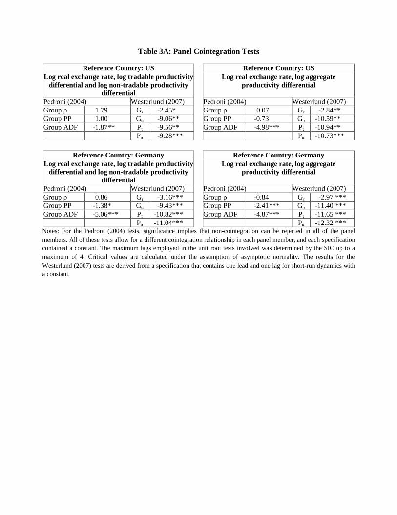
Table 3A: Panel Cointegration Tests

Reference Country: US Reference Country: US



differential




Group ρ 1.79 Gτ -2.45 * Group ρ 0.07 Gτ -2.84 **

Group PP 1.00 Gα -9.06 ** Group PP -0.73 Gα -10.59 **

Group ADF -1.87 ** Pτ -9.56 ** Group ADF -4.98 *** Pτ -10.94 **

Pα -9.28 *** Pα -10.73 ***

Reference Country: Germany Reference Country: Germany



differential




Group ρ 0.86 Gτ -3.16 *** Group ρ -0.84 Gτ -2.97 ***

Group PP -1.38 * Gα -9.43 *** Group PP -2.41 *** Gα -11.40 ***

Group ADF -5.06 *** Pτ -10.82 *** Group ADF -4.87 *** Pτ -11.65 ***

Pα -11.04 *** Pα -12.32 *** Notes: For the Pedroni (2004) tests, significance implies that non-cointegration can be rejected in all of the panel

members. All of these tests allow for a different cointegration relationship in each panel member, and each specification

contained a constant. The maximum lags employed in the unit root tests involved was determined by the SIC up to a

maximum of 4. Critical values are calculated under the assumption of asymptotic normality. The results for the

Westerlund (2007) tests are derived from a specification that contains one lead and one lag for short-run dynamics with

a constant.

38

Table 4A: Fixed-Effect Panel DOLS

Panel A: US as base country


Dependent Variable:

log RER

log tradables


log non-tradables


log aggregate


-0.44 ** 0.90 ** 0.11

(0.17 ) (0.36 ) (0.20 )

Panel B: Germany as base country


Dependent Variable:

log RER

log tradables


log non-tradables


log aggregate


-0.11 0.25 -0.10

(0.08 ) (0.27 ) (0.15 )


confidence level. Newey-West standard errors with three lags are given in parentheses.

Table 5A: Pooled Mean-Group (PMG)



Dependent Variable:

log RER

log tradables


log non-tradables


log aggregate


-0.40 *** 0.66 ** 0.20

(0.12 ) (0.26 ) (0.18 )



Dependent Variable:

log RER

log tradables


log non-tradables


log aggregate


-0.12 *** 0.15 * -0.14 **

(0.02 ) (0.08 ) (0.06 ) *: Significant at the 10% confidence level. **: Significant at the 5% confidence level. ***: Significant at the 1%

confidence level. Standard errors are given in parentheses.

39

Table 6A: Group-Mean Panel DOLS



Dependent Variable:

log RER

log tradables


log non-tradables


log aggregate


Group-mean panel

DOLS estimator

-1.09 *** 0.69 *** 0.88 ***

(0.23 ) (0.17 ) (0.28 )

Austria -2.60 3.74 2.76 *

(1.80 ) (3.84 ) (1.53 )

Belgium -0.60 1.80 1.31

(0.59 ) (1.83 ) (1.50 )

Canada 1.12 ** -2.64 1.72 *

(0.52 ) (2.15 ) (0.88 )

Denmark -4.60 *** 0.94 1.14

(0.86 ) (0.81 ) (1.21 )

Finland -0.21 0.80 -0.21

(0.72 ) (0.92 ) (0.40 )

France -2.38 ** 1.53 1.64

(1.05 ) (1.10 ) (1.15 )

Germany -0.59 0.03 1.38

(0.45 ) (1.06 ) (1.63 )

Italy 0.31 -0.54 0.69

(0.77 ) (1.32 ) (0.86 )

Japan -1.62 * 3.94 *** 3.03 ***

(0.89 ) (0.53 ) (0.63 )

Korea -0.67 *** 0.98 ** -0.17

(0.22 ) (0.42 ) (0.16 )

Netherlands -0.85 1.87 -0.29

(0.83 ) (1.67 ) (0.95 )

Norway 1.25 -5.54 0.16

(0.99 ) (4.68 ) (0.34 )

Portugal -2.44 3.71 ** 1.84 ***

(1.65 ) (1.38 ) (0.63 )

Sweden -1.29 * -0.18 -1.71 **

(0.71 ) (1.65 ) (0.63 )

United Kingdom -1.12 -0.03 -0.17

(0.99 ) (0.72 ) (0.75 )


confidence level. Newey-West standard errors with three lags and the degrees-of-freedom corrections are given in

parentheses.

40



Dependent Variable:

log RER

log tradables


log non-tradables


log aggregate


Group-mean panel

DOLS estimator

-0.20 0.49 *** 0.62 ***

(-0.11 ) (0.13 ) (0.10 )

Austria 0.60 *** 0.80 *** 1.64 ***

(0.05 ) (0.11 ) (0.13 )

Belgium -0.20 -0.91 -0.74 *

(0.12 ) (0.60 ) (0.41 )

Canada -2.83 * -0.02 2.62 **

(1.45 ) (1.14 ) (1.20 )

Denmark 0.25 *** 0.53 0.88 **

(0.06 ) (0.47 ) (0.33 )

Finland -0.43 *** 2.74 ** -0.76 ***

(0.08 ) (1.21 ) (0.27 )

France -0.06 0.07 0.18

(0.08 ) (0.26 ) (0.23 )

Italy 0.10 0.18 0.79

(0.37 ) (0.90 ) (0.78 )

Japan 0.73 1.70 2.02 ***

(0.54 ) (1.35 ) (0.48 )

Korea 0.05 -0.68 -0.16

(0.17 ) (0.69 ) (0.11 )

Netherlands -0.92 ** -0.25 0.20

(0.41 ) (0.27 ) (0.21 )

Norway 0.01 1.78 *** -0.25

(0.09 ) (0.55 ) (0.28 )

Portugal 0.74 *** -0.74 1.21 ***

(0.16 ) (0.55 ) (0.19 )

Sweden -0.37 *** 0.01 -0.97 ***

(0.11 ) (0.51 ) (0.31 )

United Kingdom -0.07 2.14 *** 1.28 **

(0.22 ) (0.57 ) (0.62 )

United States -0.59 0.03 1.38

(0.45 ) (1.06 ) (1.63 ) *: Significant at the 10% confidence level. **: Significant at the 5% confidence level. ***: Significant at the 1%

confidence level. Newey-West standard errors with three lags and degrees-of-freedom corrections are given in

parentheses.

41

Charts 1a and 1b: Mean Group Estimates of the Long-Run Coefficients of the Tradable and Nontradable

Productivity Differentials on the Real Exchange Rate (World Based and U.S. Based)

Documents

The Harrod-Balassa-Samuelson Effect: Reconciling the Evidence · Preliminary version Please do not quote without permission The Harrod-Balassa-Samuelson Effect: Reconciling the Evidence