1  

The General Equilibrium Impacts ofUnemployment Insurance: EvidencefromaLargeOnlineJobBoard1IoanaMarinescu, UniversityofChicago

AbstractDuring  the Great Recession, U.S. unemployment benefits were  extended by  up  to  73 weeks.  Theory 

predicts that extensions increase unemployment by discouraging job search, a partial equilibrium effect. 

Using data  from  the  large  job board CareerBuilder.com,  I  find  that a 10%  increase  in benefit duration 

decreased state‐level job applications by 1%, but had no robust effect on job vacancies. Job seekers thus 

faced  reduced  competition  for  jobs, a general equilibrium effect. Calibration  implies  that  the general 

equilibrium effect reduces the impact of unemployment insurance on unemployment by 40%: increasing 

benefit duration by 10% increases unemployment by only 0.6% in equilibrium. 

Keywords: unemployment insurance; job search; applications; vacancies. 

JEL: J6.   

                                                            1 I would like to thank Sanggi Kim and Sarah Sajewski for excellent research assistance. 

  

2  

1. IntroductionDuring the Great Recession, the duration of unemployment benefits in the US was extended from 26 to 

up  to  99 weeks.  A  vast  amount  of  empirical  evidence  based  on  prior  extensions  in  unemployment 

benefits  unambiguously  shows  that  extensions  increase  the  unemployment  duration  of  benefit 

recipients  (e.g. Katz and Meyer 1990; Meyer 2002; Schmieder, Wachter, and Bender 2012). Empirical 

evidence from the Great Recession in the US confirms the prevailing wisdom by showing that extensions 

had a positive effect on the unemployment duration of likely benefit recipients (Rothstein 2011; Farber 

and  Valletta  2013).  Since  extensions  contribute  to  increasing  unemployment  in  a  situation  where 

unemployment  is  already high,  there  is  a  legitimate  concern  that unemployment benefits extensions 

may have been a bad policy choice. 

However, the partial equilibrium effect of benefit extensions on benefit recipients does not capture the 

full  impact  of  the  extensions  on  aggregate  unemployment  during  the  Great  Recession.  Indeed, 

unemployment  benefit  extensions  could  also  have  general  equilibrium  effects  through  search 

externalities.  Theoretically,  as  unemployment  benefit  recipients  reduce  their  job  search  effort  in 

response to the extensions, competition for  jobs decreases and  it becomes easier for unemployed  job 

seekers who  are not  affected by  the  extensions  to  find  a  job.  Levine  (1993)  and  Lalive,  Landais,  and 

Zweimüller  (2013)  document  empirically  the  presence  of  such  search  externalities  for US  extensions 

prior  to  the  Great  Recession,  and  for  Austrian  extensions  respectively.  Even  for  benefit  recipients 

themselves, UI benefit extensions can  increase the  job finding rate per application. Thus, a UI  induced 

decrease in applications leads to a less than proportional decrease in job finding for UI recipients.  Due 

to  this search externality,  the  impact of  the extensions on aggregate unemployment could be smaller 

than the partial equilibrium impact of increasing potential benefit duration for a small number of benefit 

recipients.  

Extensions  could  also  have  general  equilibrium2  effects  through  firm  behavior,  generating  a  labor 

demand externality. If benefit extensions reduce the number of applicants for each job, it may become 

harder  for  firms  to  fill  job  vacancies,  and  the  value  of  vacancies may  decrease.  Extensions  can  also 

decrease  the  value  of  vacancies  by  increasing  the  reservation  wage  of  benefit  recipients,  so  that 

employers  face more demanding applicants.  If extensions decrease  the value of a vacancy,  firms may 

post fewer  job vacancies. A decrease  in the number of vacancies makes  it harder for all  job seekers to 

                                                            2 General equilibrium is used here as in labor economics (e.g. Landais, Michaillat, and Saez, 2014) to mean that the extensions generate externalities in the labor market. It does not mean to imply that we will analyze the impact of the extensions on markets other than the labor market. 

  

3  

find a job. Through this labor demand externality, extensions contribute to further increasing aggregate 

unemployment.  Hagedorn  et  al.  (2013)  show  evidence  that  extensions  during  the  Great  Recession 

decreased  the  number  of  vacancies,  suggesting  that  the  impact  of  the  extensions  on  aggregate 

unemployment  during  the Great  Recession  is  larger  than  the  impact  of  these  extensions  on  benefit 

recipients. 

However,  whether  the  negative  impact  of  extensions  on  the  number  of  vacancies  (labor  demand 

externality) dominated the positive  impact of extensions on  job  finding (search externality) during the 

Great Recession  is unknown.  In particular, while Hagedorn et al. (2013) provide evidence on the  labor 

demand externality, we have no evidence on  the  search externalities generated by extensions during 

the Great Recession. Therefore, whether the macro impact of extensions on aggregate unemployment is 

larger or smaller than the micro effect on benefit recipients remains an open question.  

To answer this question, this paper uses new data on state‐level job applications and job vacancies from 

CareerBuilder.com,  arguably  the  largest  American  online  job  board3.  If  extensions  during  the  Great 

Recession  resulted  in a decrease  in aggregate  job  search effort, we  should observe a decrease  in  the 

total number of job applications in the aftermath of an extension. All other things equal, such a decrease 

in  job  applications  increases  the  hiring  rate  per  application  sent,  a  search  externality,  and  therefore 

contributes to reducing unemployment. I can also ascertain whether extensions decreased the number 

of  job  vacancies  posted,  a  labor  demand  externality,  and  therefore  contributed  to  increasing 

unemployment. Thus, a key innovation of this paper is to estimate the impact of extensions on both job 

applications and job vacancies during the Great Recession.  

If extensions reduce the total number of job applications more than they reduce the total number of job 

vacancies,  then  extensions  increase  the  vacancy  to  applications  ratio  (a measure  of  search‐intensity 

adjusted labor market tightness), and therefore increase the job finding probability per application sent. 

In this case, economic theory predicts that the macro impact of extensions on aggregate unemployment 

is  smaller  than  the micro  impact on  the unemployment of benefit  recipients  (Landais, Michaillat, and 

Saez, 2014), so that the general equilibrium effect dampens the partial equilibrium effect. Conversely, if 

benefit extensions decrease labor market tightness, then the macro impact of extensions on aggregate 

unemployment is larger than the micro impact on benefit recipients.  

                                                            3 Monster.com  is  similar  in  size,  and whether Monster  or  CareerBuilder  is  largest  depends  on  the  exact  size measure used. 

  

4  

To  identify  the  impact  of  unemployment  insurance  on  applications  and  vacancies,  I  use  state‐level 

variation  in  potential  unemployment  benefits  duration  (PBD)  induced  by  the  federal  Emergency 

Unemployment  Compensation  (EUC)  and  state‐run  extended  benefits  (EB).  My  first  identification 

strategy is a timing of events approach, and shows that the number of vacancies in the state stays flat as 

far  as  seven months before  and  after  a  state’s  largest benefit  extension. By  contrast,  state‐level  job 

applications significantly decline  in  the  first month of a benefit extension, and continue  to decline  for 

several months thereafter. Using this strategy, a one‐week  increase  in potential benefit duration (PBD) 

leads to a 0.4% decline in applications at the state level. Equivalently, a 10% increase in PBD decreases 

state‐level applications by 1% (an elasticity of ‐0.1). 

A second identification strategy uses the fact that benefit extensions (EUC and EB) depend on state‐level 

unemployment  rates  reaching  specific  thresholds.  I  exploit  this  source  of  variation  by  using  a  global 

parametric fuzzy regression discontinuity approach that relies on nonlinearities  in PBD as a function of 

the state unemployment  rate.  I  find  that PBD decreases  the  total number of applications at  the state 

level, but has no robust impact on the number of vacancies. Furthermore, only the federal EUC program 

has a negative  impact on PBD, while  the  state‐level EB has no  significant effect. Overall,  this  second 

identification  strategy confirms  that PBD extensions decrease  the  total number of applications at  the 

state level, but have no robust impact on the number of vacancies. 

One may be concerned that the impact of PBD extensions on job applications and vacancies is biased by 

the  lack of representativity of my data or by unobserved changes  in the composition of  job vacancies. 

However, I show that the negative impact of PBD on applications is robust to controlling for changes in 

the composition of job vacancies by  industry and education requirement. I also show that the absence 

of  an  impact  of  PBD  on  vacancies  is maintained when  using  all  online  vacancies  from Help Wanted 

Online rather than just CareerBuilder vacancies. Finally, I find that PBD does not affect posted wages or 

how  choosy  job  seekers  are.  The  lack  of  an  impact  of  extensions  on  posted wages  and  job  seeker 

choosiness  is  consistent with  the  fact  that  extensions  do  not  affect  the  number  of  vacancies:  since 

extensions  do  not  have  an  impact  on  how  choosy  job  seekers  are  nor  posted wages,  they  do  not 

contribute to decreasing the value of vacancies. 

In contrast to my results, Hagedorn et al. (2013) found a negative  impact of unemployment  insurance 

extensions on vacancies during the Great Recession. Hagedorn, Manovskii, and Mitman (2016) suggest 

that  the difference between our  results  is due  to a difference  in data  source. However,  I  still  find no 

effect of the extensions on the number of vacancies when using the Help Wanted Online data with my 

  

5  

identification  strategy. Their  identification  strategy  relies on  comparing  counties  along  state borders. 

Borrowing their identification strategy and using county level data, I find no effect of the extensions on 

vacancies.  Furthermore,  I  show  that  the  border  county  design  cannot  recover  the  causal  impact  of 

unemployment  insurance  on  applications  and  vacancies  due  to  large  across‐county  spillover  effects. 

More generally, these results suggest that one should be wary of using border county designs to assess 

the impact of labor market policies that have geographic spillover effects. 

Overall,  this paper’s main  empirical  results  are  informative  about  the  general  equilibrium  impacts of 

unemployment  insurance:  they  indicate  that  unemployment  insurance  extensions  during  the  Great 

Recession did not lead to a labor demand externality (no impact on the number of vacancies or posted 

wages), but did generate a job search externality (a negative impact on the number of applications). On 

net, extensions had a positive and significant impact on labor market tightness, implying that the macro 

effect of unemployment  insurance on unemployment  is smaller  than  the micro effect. This  result has 

important implications for policy design. Indeed, to the extent that labor market tightness is inefficiently 

low  during  recessions  and  inefficiently  high  during  booms,  the  fact  that  unemployment  insurance 

increases  labor market  tightness  implies  that optimal unemployment  insurance  generosity  should be 

high in recessions and low in booms, i.e. countercyclical (Landais, Michaillat, and Saez 2014).  

To quantify the macro impact of unemployment insurance, I calibrate the theoretical model by Landais, 

Michaillat, and Saez 2014  in which  this macro  impact  is  the sum of  the micro  impact and  the general 

equilibrium effect. I find that the macro impact is smaller than the micro impact: the general equilibrium 

effect  reduces  the micro  impact  by  40%.  In  equilibrium,  a  10%  increase  in  unemployment  benefit 

duration increases aggregate unemployment by only 0.6%. 

The  remainder of  the  paper  is organized  as  follows.  Section  2 discusses how unemployment benefit 

extensions  were  decided,  describes  the  data  and  presents  the  theoretical  framework.  Section  3 

discusses  the  identification  strategy  and  the  results  for  the  timing  of  events  approach,  and  the 

parametric fuzzy regression discontinuity designs. Section 4 presents robustness tests and discusses the 

results.  In  particular,  section  4  presents  the  calibration  results  for  the  impact  of  PBD  extensions  on 

aggregate unemployment. Section 5 presents interpretations and discussion of findings. Finally, Section 

6 concludes. 

  

6  

2. Policybackground,data,andtheoreticalframework

2.1Policybackground

By default, PBD  in  the United States  is 26 weeks. During  times of high unemployment,  the extended 

benefits (EB) program provides additional weeks of benefits if one of two conditions is satisfied:  

the state's 13‐week average insured unemployment rate (IUR) in the most recent 13 weeks is at 

least 5.0 percent and at least 120 percent of the average of its 13‐week IURs in the last 2 years 

for the same 13‐week calendar period; or  

at state option, the current 13‐week average  IUR  is at  least 6.0 percent, and regardless of the 

experience in previous years. The IUR option is in place for the months when a state chose this 

option4. 

States have the option of electing an alternative trigger authorized by the Unemployment Compensation 

Amendments of 1992  (Public  Law 102‐318). The TUR option  is  in place  for  the months when a  state 

chose  this  option.  This  trigger  is  based  on  a  3‐month  average  total  unemployment  rate  (TUR)  using 

seasonally adjusted data: 

If  this TUR  average exceeds 6.5 percent  and  is  at  least 110 percent of  the  same measure  in 

either of the prior 2 years, a state can offer 13 weeks of EB.  

If the average TUR exceeds 8 percent and meets the same 110‐percent test, 20 weeks of EB can 

be offered. 

Normally, extended benefits are financed 50% by states and 50% by the federal government. Under the 

American Recovery and Reinvestment Act of 2009 (ARRA) passed on Feb. 17, 2009, benefits are financed 

entirely by the federal government. As a result, many states chose the TUR option5. Federal funding of 

EB was still in place at the end of this paper’s sampling frame (July 2011).  

The  Tax  Relief,  Unemployment  Insurance  Reauthorization,  and  Job  Creation  Act  of  (P.L.  111‐312, 

December  2010)  temporarily  changed  the  look‐back  timeframe  to  three  years,  as  unemployment 

                                                            4 78% of states choose this option, and this share is stable over the sample frame of this paper. 5  In  this paper’s  sample  frame, and before ARRA, only 21% of  state‐week observations had  the TUR option on, while after ARRA 63% of  state‐week observations had  the TUR option on. As of  January 2011, Arkansas,  Iowa, Louisiana, Maryland, Mississippi, Montana, Oklahoma, Utah, and Wyoming could qualify for extended benefits (EB) under TUR but chose not to use that option. Legislators in these states were afraid of adopting extended benefits under TUR because they were afraid of having to raise taxes when the federal funding expires. Furthermore, many legislators were afraid that more benefits would increase unemployment. 

  

7  

indicators  in most states had been consistently high for the past two years and would have resulted  in 

many states being unable to meet the conditions. This three‐year look‐back exception was still in place 

at the end of the sampling frame (July 2011). 

The federal Emergency Unemployment Compensation Act (EUC) 2008 further extended benefits. EUC‐08 

is an emergency federal benefits program that is payable to individuals who have exhausted all rights to 

regular compensation with  respect  to a benefit year  that ended on or after May 1, 2007. Typically, a 

jobseeker collects EUC benefits before EB benefits. EUC evolved in the following way: 

The EUC08 program (June 30, 2008), provides up to 13 weeks of 100 percent federally‐financed 

compensation  in  all  states.  Public  Law  (P.L.)  110‐449  expanded  the  EUC08  program  on 

November 21, 2008 to provide up to 20 weeks of benefits. This constitutes tier 1 or EUC1. 

Tier 2 of EUC (EUC2) was created by Public Law (P.L.) 110‐449. It provides 13 weeks of benefits 

in states where TUR (defined as for EB) is above 6% or IUR (defined as for EB) is above 4%. 

Public Law No. 111‐92, enacted on November 6, 2009, expanded the EUC08 program: 

o It  increased the maximum EUC2 entitlement from 13 weeks to 14 weeks of benefits  in 

all states, and established  that  this Tier was no  longer  triggered by a state  reaching a 

specified rate of unemployment; 

o  It created EUC3 providing up to 13 additional weeks of benefits in states with IUR above 

4 percent or TUR above 6 percent; 

o It created EUC4 providing up to 6 additional weeks of benefits in states with IUR above 6 

percent or TUR above 8.5 percent. 

The impact of the EUC and EB extensions on the job search effort of benefit recipients may be different 

for three reasons. First, because EB benefits only become available after workers have exhausted their 

regular  and  EUC  benefits,  the  impact  of  EB  on  job  search  is  likely  to  be  smaller  due  to  discounting. 

Second,  EB  has  more  stringent  job  search  requirements  than  EUC  (see  Federal‐State  Extended 

Unemployment Compensation Act of 1970), so EB may have a lower impact on job search effort.  Third, 

the estimated  impact of EB and EUC could differ because EB partially depends on states’ choice while 

EUC does not. Therefore, some of the variation in weeks of EB may be endogenous: for example, states 

with high unemployment prospects may choose to provide more EB by adopting the TUR option. Since 

estimated impact of EUC and EB on aggregate job search effort may be different, I will be investigating 

the contrasting effects of EUC and EB. 

  

8  

For both EUC and EB, TUR conditions are much more  likely to be satisfied than the IUR conditions. For 

example, EUC2 and EUC3 require that TUR be above 6% or IUR above 4%. In the data sample, when TUR 

is above 6%,  IUR  is above 4%  in 97% of  the cases. On  the other hand, when  IUR  is below 4%, TUR  is 

nonetheless above 6% in 54% of the cases. If TUR is below 6%, IUR is above 4% in only 1.8% of cases, so 

IUR is unlikely to trigger increases in PBD. 

Since  the  conditions  governing  the  maximum  weeks  of  UI  benefits  are  fairly  complex,  Figure  1 

summarizes  the  regulation  in  a  simplified  form.  The  figure  ignores  some  of  the  finer  points  of  the 

regulation discussed above and simply shows how PBD depends on TUR during different  time  frames 

and  in states that had the TUR option  for EB (i.e. the majority of states). This overview of the policies 

suggests that one can use sharp changes  in benefit duration at 6.5% and 8% TUR (for EB) and 6% and  

8.5% TUR (for EUC) to identify the impact of benefit duration on applications and vacancies. 

2.2Data

The  data  on  applications  and  job  vacancies  comes  from  proprietary  data  provided  to  me  by 

CareerBuilder.com. Job vacancies are defined as the total number of online  job advertisements posted 

by firms  in a given state during a given month. CareerBuilder charges firms several hundred dollars to 

post a  job ad on the website for one position for one month. A  firm that wishes to advertise multiple 

positions needs to pay for each position separately, though quantity discounts are available. By contrast, 

the service is free for job seekers. 

One can compare  job vacancies  in CareerBuilder.com with data on  job vacancies  in the representative 

JOLTS  (Job  Openings  and  Labor  Turnover  Survey).  The  number  of  vacancies  on  CareerBuilder.com 

represents  35%  of  the  total  number  of  vacancies  in  the  US  in  January  2011  as  counted  in  JOLTS. 

Compared  to  the  distribution  of  vacancies  across  industries  in  JOLTS,  some  industries  are 

overrepresented in CareerBuilder data, in particular information technology, finance and insurance, and 

real estate, rental and  leasing. The most underrepresented  industries are state and  local government, 

accommodation and food services, other services, and construction. When comparing the distribution of 

jobs  across US  regions  in  JOLTS  vs  CareerBuilder,  I  find  that  CareerBuilder  has  the  same  geographic 

  

9  

distribution  of  jobs  as  JOLTS.    As  for  the  time  series  properties  of  the  CareerBuilder  vacancy  data, 

vacancies in CB follow very closely the trends in the JOLTS data6 (correlation of 0.57, P‐value<0.01). 

In Marinescu and Rathelot  (2014), we use a  representative sample of vacancies and  job seekers  from 

CareerBuilder.com  in  2012.  The  distribution  of  vacancies  across  occupations  is  essentially  identical 

(correlation of 0.95) to the distribution of vacancies across all  jobs on the  Internet as captured by the 

Help  Wanted  Online  data.  Furthermore,  the  distributions  of  unemployed  job  seekers  on 

CareerBuilder.com across  states and occupations are  similar  to  those of  the nationally  representative 

Current Population Survey  (correlations of more  than 0.7).   Overall,  the vacancies and  job seekers on 

CareerBuilder.com  are  broadly  representative  of  the  US  economy  as  a  whole,  and  they  form  a 

substantial fraction of the market. 

In  the CareerBuilder data,  for each  state,  information  is available on  the distribution of  vacancies by 

industry, the  level of education required7, and the posted wage. The posted wage  is reported  in seven 

bins8, and, when a wage range is offered, these bins are based on the upper bound of the offered wage. 

Among vacancies that post a wage, the median is $50,000: indeed, 52% of vacancies with posted wages 

post a wage of $50,000 or more. This median wage  is somewhat higher  than  the $45,230 US average 

wage  in 2011  (BLS Occupational Employment Statistics), but again  the CareerBuilder  compensation  is 

based on the upper bound of the offered wage.  

The CareerBuilder data  spans September 2007  to  July 2011.   An  individual application  is defined as a 

person clicking on  the “Apply Now” button  in a  job ad9. The variable “Applications”  is  the number of 

individual applications received by all jobs in a given state and month.  

The  recorded  applications  are  from  any  job  seeker,  including unemployment benefit  recipients, non‐

employed job seekers who do not receive unemployment benefits, and employed workers. According to 

                                                            6 Labor market tightness as measured by  log(jobs  in JOLTS)‐log(unemployed  in CPS)  is also highly correlated with search  intensity  adjusted  labor  market  tightness  measured  as  log(jobs  on  CareerBuilder)‐log(applications  on CareerBuilder). The correlation is 0.57, P‐value<0.01. 7 When  there  is  no  education  requirement,  it  just means  that  the  field was  not  filled  by  the  employer.  The employer can still specify an education requirement within the text of the ad. 8 The wage bins are: $1‐$30000, $30001‐$50000, $50001‐$75000, $75001‐$100000, $100001‐$200000, $200001‐$500000, higher than $500000. 9 Tracking cookies, resumes, and other variables are ways that CareerBuilder limits the ability for any job seeker to apply to the same job more than once. 

  

10  

CarrerBuilder’s applicant survey, just under half of the applicants are employed10. Therefore, given that 

applications by non‐UI recipients constitute a substantial share of total applications, if we only had data 

on the applications of UI recipients, we would not be able to adequately quantify the impact of PBD on 

labor market tightness. Because we have the number of vacancies as well as the number of applications 

to these vacancies coming from all types of job seekers, this data is uniquely suited to study the impact 

of PBD on labor market tightness.  

To reproduce the border‐county design used by Hagedorn et al. (2013) to identify the impact of PBD on 

vacancies, I exploit an additional sample that aggregates vacancies and applications at the county level 

rather  than at  the state  level. To  identify border counties,  I use  the publicly available border counties 

pair data from Dube, Lester, and Reich (2010).   

To determine how many weeks of extended benefits are effectively available for each state and week, I 

use data from the Department of Labor EB and EUC trigger notices. These notices report the Potential 

benefit duration (PBD)  in weeks, which  is an upper bound on the duration of UI for two reasons. First, 

regulations  entail  lower  maximum  durations  for  some  workers,  in  particular  those  who  have  only 

worked for a short period of time prior to becoming unemployed11. Second, many job seekers find a job 

early and do not  receive  the maximum possible duration of benefits. Trigger notices also contain  the 

TUR,  IUR, and  look‐back criteria. This allows me to determine when the conditions  for each extension 

are realized. Since this data has weekly frequency while the CareerBuilder data has monthly frequency, I 

take the monthly average of the PBD,  IUR and TUR to merge  it with the monthly data on applications 

and vacancies.  

Data  from  the Bureau of Labor Statistics was used  to  supplement  the above  information on  jobs and 

jobseekers. First, I use data on the total number of unemployed people and the labor force (Labor Force 

Statistics from the Current Population Survey). Second,  I use data on vacancies and hires from the Job 

Openings and Labor Turnover Survey (JOLTS).  

Table 1  shows  summary  statistics  for key variables. Particularly noteworthy are  the  large numbers of 

applications per state. The number of CareerBuilder applications is about twice as high as the number of 

unemployed  individuals  in  the  state;  on  average,  each  vacancy  receives  about  30  applications  per 

                                                            10 This statistic  is  interesting but cannot be taken at face value since  it  is based on the selected sample of those applicants who were willing to answer the survey. 11 Benefit durations are capped through the maximum total amount that people can collect based on their prior earnings (Meyer 2002). 

  

11  

month. Figure 2 shows the evolution of the unemployment rate, job vacancies (from Job Openings and 

Labor Turnover Survey) and PBD at the national level. This graph shows that PBD and unemployment are 

positively correlated, consistent with the fact that PBD is increased when unemployment exceeds some 

thresholds.  

2.3Theoreticalframework

An increase in PBD increases the unemployment duration of UI recipients (e.g. Katz and Meyer 1990; J. 

F. Schmieder, Wachter, and Bender 2012; Rothstein 2011; Farber and Valletta 2013), chiefly because of 

a decrease in job search effort rather than an increase in the reservation wage (Card, Chetty, and Weber 

2007; Lalive 2007; van Ours and Vodopivec 2008; Krueger and Mueller 2011; J. Schmieder, von Wachter, 

and  Bender  2012)12.  Therefore, we  expect  the  number  of  job  applications  sent  by  UI  recipients  to 

decrease when PBD  increases and, hence, we expect  the unemployment duration of UI  recipients  to 

increase. This phenomenon is the micro or partial equilibrium effect.  

But  what  is  the  impact  of  a  decrease  in  applications  coming  from  UI  recipients  on  the  aggregate 

unemployment rate? To estimate  the macro effect of unemployment  insurance, we need  to take  into 

account general equilibrium effects through job search and labor demand externalities. If the number of 

vacancies stays the same, then the decrease  in applications by UI recipients decreases competition for 

jobs.  This  decrease  in  the  competition  for  jobs  increases  the  chances  of  finding  a  job  for  non‐UI 

recipients  (Levine  1993;  Lalive,  Landais,  and  Zweimüller  2013).  Furthermore,  this  decrease  in  the 

competition  for  jobs will  also  increase  the  rate  at which UI  recipients  find  jobs  for  each  application 

made. Therefore, this job search externality dampens the impact of UI on aggregate unemployment.  

However, since a lower number of applications per vacancy reduces an employer’s choices for potential 

hires, it may discourage further vacancy creation. Moreover, if PBD increases the reservation wage, this 

may  discourage  vacancy  creation  as  employers  may  not  be  able  to  meet  the  wage  demands  of 

applicants.  If  fewer vacancies are created, all  job seekers  find  it more difficult  to get a  job. This  labor 

demand externality  amplifies  the  impact of UI on  aggregate unemployment.  Therefore,  if  the  search 

externality dominates,  the macro  impact of UI on aggregate unemployment  is smaller  than  the micro 

effect, while the opposite is true if the labor demand externality dominates. 

                                                            12 The impact of unemployment insurance on re‐employment wages or reservation wages is estimated to be close to zero by this literature. Lalive, Landais, and Zweimüller (2013) and Nekoei and Weber (2013) are the exceptions to the rule and find a small positive impact of unemployment insurance extensions on re‐employment wages. 

  

12  

Landais, Michaillat,  and  Saez  (2014)  formalize  this  reasoning  and  show  that,  when  unemployment 

insurance increases labor market tightness, the macro effect is smaller than the micro effect, and vice‐

versa when unemployment insurance decreases labor market tightness. Furthermore, they demonstrate 

that  optimal  unemployment  insurance  should  be  countercyclical  if  the  elasticity  of  labor  market 

tightness with respect to unemployment benefits is positive, and pro‐cyclical otherwise. 

Here, the generosity of unemployment benefits is measured by potential benefit duration (PBD). If PBD 

increases labor market tightness, then the impact of PBD on aggregate unemployment is lower than the 

impact of PBD on the unemployment of UI recipients, and the opposite  is true  if PBD decreases  labor 

market tightness. I will estimate the impact of PBD on log vacancies, log applications, and log tightness 

(log vacancies‐log applications). If the impact of PBD on tightness is positive, then the macro impact of 

PBD is lower than its micro impact, and optimal unemployment benefit duration is counter‐cyclical. 

3. Mainresults

3.1Timingofeventsapproach

The timing of events approach uses the timing of PBD increases at the state level to identify the impact 

of  PBD  on  applications  and  vacancies.  If  PBD  has  a  negative  impact  on  job  search  as measured  by 

applications, we expect the number of applications to significantly drop  in the first month after a PBD 

increase. More generally,  if PBD has an  impact on  the outcome of  interest,  then  this outcome should 

vary over time in the same way as PBD at the state level. The key identification assumption is that there 

is no omitted variable  that evolves according  to  the same monthly  timing as PBD and determines  the 

outcome of interest.  

3.1.1Methodologyfortimingofeventsapproach

For  each  state,  I  identify  the  largest  increase  in  PBD13  that  is  not  due  to  a  change  in  the  benefit 

schedule14 (see Figure 1) nor to a temporary lapse in EUC15. Emphasis is placed on the largest increase in 

                                                            13 The date of the largest increase in PBD and the amount of the increase for each state can be found in Appendix 1, Table 8. 14 This is because changes in schedule yield the largest increases in PBD for most states, but they all happen at the same time, which makes it impossible to separate the impact of PBD from a pure time effect. 15 During the sample period, there were two lapses in extended benefits because legislators struggled to reach an agreement. These two lapses were in April to July 2010 and in November‐December 2010. Ultimately, any benefits lost from these lapses were reinstated once the legislative agreement was reached. There was little reaction of job applications to these EUC lapses (Appendix 1, Figure 5); presumably, jobseekers were expecting these EUC lapses to be temporary. 

  

13  

PBD16 for two reasons. First, when there are at  least two  increases  in PBD  in a state, some months of 

observation are both after the first increase and before the second increase, which makes it difficult to 

uniquely  assign  these  observations  to  a  “before”  or  “after”  period.  Second,  given  that  it  is  more 

transparent to focus on just one increase in PBD, choosing the largest one should maximize power.  

For  each  state,  I only  keep observations  around  the  largest  increase  in  PBD  that do not  involve  any 

further change in PBD. As a result of this restriction, benefit duration is constant during the months prior 

to the largest PBD increase and also constant during the months after the largest PBD increase17. I then 

use  the  following  specification  to  estimate  the  impact of  the  largest  increase  in  benefit duration on 

various outcomes: 

 

where    is  the outcome of  interest  in state   and month  .      is a dummy equal  to 1  in month   

relative to the  largest  increase  in PBD  in a given state, where  0  is the first month when the higher 

PBD is available during all weeks of the month. The dummy for month  2 is the omitted category18. 

 is a quarter fixed effect to capture seasonality.   is a year fixed effect and   is a state fixed effect. I 

cluster standard errors at the state  level. To obtain the  impact of one week of PBD on the outcome of 

interest, one can replace the    dummies by PBD. Given the sample selection, PBD is constant before 

the  largest  increase  in PBD, then goes up to a new value and stays constant. Therefore, replacing  the  

 dummies by PBD  in  this  specification  is  similar  to adding one “after  the  largest  increase  in PBD” 

dummy while allowing for a dose response effect.  

                                                            16 In Appendix 1, Table 10, I also report regression results for alternative definitions of the event (a PBD increase of 10 weeks or more and a PBD  increase of  less  than 10 weeks);  the  results are  similar  to  those obtained  for  the largest increase in PBD. 17 This restriction also implies that, in practice, we have an unbalanced panel of states (see Appendix 1, Figure 6). I also used a balanced panel sample of 18 states that have a constant PBD three months before and after the largest increase  in PBD. Using this sample, there  is a significant decline  in applications after the  largest  increase  in PBD, while there  is no significant change  in the number of vacancies (Appendix 1, Figure 7). Thus, the balanced panel results are consistent with the results from the unbalanced panel (Figure 3). 18 Because  the data on applications  is at  the monthly  level while PBD  is defined weekly,  the  largest  increase  in benefit duration defined as above will  typically occur over  three months, with  the  first month having  the  lower potential benefit duration  (PBD), the second month having a mix of  lower and higher PBD, and the third month having the higher PBD. Therefore, I use the largest increase in benefit duration relative to two months prior (e.g. May to July). Any month that contained a mix of weeks with high and low benefit levels was excluded. 

  

14  

The key assumption needed to identify the causal effect of PBD on the outcome of interest is that there 

are no omitted variables that follow the same time course as PBD around the maximum increase in PBD 

and  affect  the outcome of  interest.  This  assumption  is made more  likely by  the  fact  that  these PBD 

increases occur at different times in different states and are mostly driven by states crossing thresholds 

in the state unemployment rate (TUR or IUR) that qualify them for additional weeks of benefits19. 

As an additional  robustness  test,  I add  to  the sample a control group  for each state. For each state,  I 

added all  the states  that had a constant PBD around  the  time of  that state’s  largest PBD  increase20.  I 

define an experiment   as the set of observations that  includes a state X around  its  largest  increase  in 

PBD, as well as all the control states for that particular state X. One single natural experiment   allows 

for a classic difference‐in‐differences specification. Here I am stacking all these difference‐in‐differences 

regressions  for  all  the  states.  The  stacked  difference‐in‐differences  specification  is  then  defined  as 

follows: 

 

  is  the  outcome  of  interest  in  experiment  ,  state    and month  .      is  the  Potential Benefit 

Duration in weeks,   is a quarter fixed effect to capture seasonality,   is a year fixed effect.   is a 

dummy  for  the date being after the  largest  increase  in PBD  in experiment  .      is an experiment by 

state  fixed effect. Each state will appear at  least once, during  the time when  it experiences  its  largest 

increase  in PBD. Furthermore, each state appears whenever  it can serve as a control for another state 

experiencing  its  largest  increase  in PBD:  thus,  there  can be multiple observations  for each  state  and 

month. Therefore,    is the error term, and standard errors are clustered by state.  I  include the PBD 

  rather  than  the  interaction  between  a  treatment  dummy  and  an  after  dummy  (as  would  be 

standard  for  a  difference‐in‐differences  specification)  to  allow  for  a  dose  response  reaction,  i.e.  to 

quantify the impact of a one week increase in PBD on the outcomes of interest. 

This  difference‐in‐differences  specification  can  control  for  variation  over  time  in  the  outcomes  of 

interest  that  is  unrelated  to  PBD  and  is  common  between  treatment  and  control  states.  The  key 

assumption needed to identify the causal effect of PBD on the outcome of interest is that control states 

                                                            19 In a minority of states (20%), the largest increase is due to the state adopting the TUR option. 20 On average, each state has 21 control states. 

  

15  

are a valid counterfactual  for treated states  (common trends assumption21).  If an unobserved variable 

exists that follows the same time course as PBD around the maximum  increase  in PBD and affects the 

outcome of interest, then this variable should also affect the control states. Therefore, the difference‐in‐

differences specification serves as a robustness test on the simple timing of events approach. 

3.1.2Resultsfromthetimingofeventsapproach

I  start by  showing graphically how applications evolved around  the  largest  increase  in PBD  (Figure 3, 

Panel A). While there was no significant trend in the number of applications prior to the largest increase 

in benefit duration, there was a significant drop  in applications during the first month  (month 0) after 

the increase in benefit duration. Given that the average increase in benefit duration was 15 weeks22, the 

estimated effect implies that a 1 week increase in PBD leads to a 0.4% decline in applications.  

Applications continues to decline after the first period post benefit increase and the impact in the third 

month  (month  2)  is  significantly  higher  than  the  impact  in  the  first month,  implying  that  a  1 week 

increase  in PBD  leads  to a 1% decline  in applications  three months after  the  increase. This decline  in 

applications after the PBD  increase  is robust to taking  into account sample selection:  if we restrict the 

sample to states that are  in the sample  in months 0, 1 and 2 (23 states), the  impact  in month 2  is still 

significantly larger than the impact in month 0. This decline in applications may be explained by the fact 

that more  and more UI  recipients  become  aware  of  the  benefit  extensions  over  time.  Indeed, most 

states only notify UI recipients of their eligibility for extended benefits once they exhaust their regular 

benefits. To summarize, I find that a PBD increase coincides with a significant decline in job applications 

in the very first month of the PBD increase and this decline deepens in following months. 

I next examine the  impact of PBD on vacancies. There  is no significant trend23  in  job vacancies around 

the largest increase in PBD (Figure 3, Panel B). This implies that, as far as seven months after the largest 

increase  in  PBD,  employers  do  not  respond  to  a  higher  PBD  by  posting  fewer  vacancies.  Since 

applications  decrease  after  the  largest  increase  in  PBD  and  vacancies  stay  constant,  labor  market 

tightness (log vacancies‐log applications) increases after the largest increase in PBD (Appendix 1, Figure 

9). 

                                                            21  In practice, applications  in  the  control  states  follow  the  same  time path prior  to  the  largest PBD  increase as applications in the treated states, and the same holds for vacancies (Appendix 1, Figure 8). Therefore, the control group seems to satisfy the common trends assumption. 22 The level of PBD around the largest increase in PBD is plotted in Appendix 1,Figure 6. 23 Even though a few pre‐event point estimates are significant, this is probably due to sampling variability as these estimates are based on fewer than 20 states (see Appendix 1, Figure 6). 

  

16  

To summarize  these graphical  results  in a  regression  format,  I use  the simple difference specification, 

which corresponds to Figure 3, and shows the average effect of one week of PBD on the outcomes of 

interest rather than estimating the  impact month by month. Consistent with the results from Figure 3, 

the simple difference specification shows a significant and negative impact of PBD on applications (Table 

2, col. 1) but no significant impact on vacancies (Table 2, col. 3). 

To test the robustness of the timing of events approach to unobserved variables that follow the same 

timing as PBD and affect  the outcomes of  interest,  I use a difference‐in‐differences  specification. The 

impact of PBD on applications remains negative and statistically significant (Table 2, column 2). Overall, 

the specifications in columns 1‐2 paint a consistent picture and indicate that a one week increase in PBD 

led to a 0.4% decline in job applications24.  

As  for  the  impact  of  PBD  on  vacancies,  the  difference‐in‐differences  specification  still  yields  an 

insignificant  effect  (Table  2,  column  4).  This  result  addresses  an  important  concern with  the  simple 

difference specification. Indeed, if there is a positive trend in vacancies, as is the case during most of the 

period when PBD  increases  (see Figure 2),  this positive  trend may be masking  the negative  impact of 

PBD on vacancies. To the extent that such a trend  is masking the negative effect of PBD on vacancies, 

the estimated impact of PBD on vacancies should become more negative when we add a control group 

of other states that share in this trend. Thus, the fact that the difference‐in‐differences specification also 

yields an insignificant impact of PBD on vacancies confirms that PBD has little if any impact on vacancies. 

Finally,  the  impact  of  PBD  on  labor market  tightness  is  positive  and  significant  both  in  the  simple 

difference and the difference‐in‐differences specification25 (Table 2, col. 5‐6). 

Using the timing of events approach,  I have shown that an  increase  in PBD has a  large, significant and 

negative  impact  on  state‐level  job  applications,  consistent with  PBD  generating  a  search  externality. 

However, PBD does not have a  robust effect on vacancies:  therefore, PBD does not generate a  labor 

demand externality.   Overall, PBD  increases  labor market  tightness. Given  the  theory outlined above, 

                                                            24 The reader may wonder why the impact on job applications is only about 0.4% given that the impact of PBD on applications  increases with  time  since  the  largest PBD  increase  (Figure 3, Panel A). This  is because  the  figure  is based on an unbalanced panel. In fact, the median state is only observed for 2 months after the PBD increase, so the regression mostly captures the short‐run effect. 25 The  impact of PBD on applications and vacancies  is  robust  to adding month  fixed effects  instead of year and quarter  fixed effects  in  the difference‐in‐differences  specification. However, because  the point  estimate of  the impact of PBD on applications  slightly decreases when month  fixed effects are  included,  the  impact of PBD on tightness falls short of statistical significance (see Appendix 1 Table 9). 

  

17  

this  implies  that  the  general  equilibrium  effects  of  unemployment  insurance  dampen  its  partial 

equilibrium effect. 

3.2Usingaparametricfuzzyregressiondiscontinuity

The first part of the analysis used a timing of events approach to  identify the causal  impact of PBD on 

applications  and  vacancies.  However,  in  such  a  design,  observations  around  the  PBD  increase  are 

associated with different unemployment  rates  for different  states. Furthermore,  the  timing of events 

approach focuses on the largest increase in PBD for each state. If heterogeneity is present in the effects 

of various PBD increases, then the timing of events approach does not adequately quantify the average 

effect  of  UI  extensions  during  the  Great  Recession.    Using  a  regression  discontinuity  design  is  an 

alternative approach that can overcome some of these limitations.  

To  exploit  the  fact  that  PBD  depends  on  states  crossing  TUR  and  IUR  thresholds,  I  use  a  global 

parametric fuzzy regression discontinuity. In Appendix 2, I also report results for a local fuzzy regression 

discontinuity  design  around  6%  TUR. While  the  local  fuzzy  regression  discontinuity  is  conceptually 

appealing,  it  leaves only  44 observations  and  therefore  very  limited  statistical power.  For  the  global 

parametric fuzzy regression discontinuity,  I use a broader sample of all the 1,804 observations  lying  in 

the zone where there are any discontinuities  in PBD as a  function of TUR  (and  IUR). Compared to the 

local fuzzy regression discontinuity design, this approach has higher power but also more potential bias 

due to the inclusion of observations that lie further away from TUR discontinuities. 

3.2.1Methodology

To  visualize  the  nonlinear  relationship  between  TUR  and  PBD  graphically,  one  can  plot  a  smoothed 

version of PBD and applications residuals or vacancies residuals as a function of TUR. The residuals are 

from regressing  log applications or  log vacancies on state fixed effects.  I then apply a kernel‐weighted 

local polynomial smoothing to the residuals26. Additionally, TUR is restricted to between 4% and 10%, so 

as to include some data prior to any TUR threshold being reached. This restriction discards data that  is 

far away from the TUR thresholds that are the primary source of identification.  

To  complement  the graphical analysis,  I  run a global parametric  fuzzy  regression discontinuity design 

that uses a broader sample. The regression discontinuity is fuzzy because crossing a threshold in TUR or 

IUR  increases  the probability of an  increase  in PBD by  less  than one due  to delays  in making benefits 

available,  conditions on  the  rate of  increase of unemployment, and  states’ policy  choices  (see policy 

                                                            26 The plot uses the Stata command lpolyci. 

  

18  

background  above).  The  design  is  global  and  parametric  because  I  include  a  range  of  observations 

around multiple  discontinuities  in  PBD  as  a  function  of  the  assignment  variables  TUR  and  IUR,  and 

control for global polynomials in TUR and IUR. 

This  approach  results  in  the  following  instrumental  variable  specification,  restricting  to  state‐month 

observations with TUR between 4 and 10%: 

 

where   is log applications, log vacancies or log tightness (log vacancies‐log applications) in state   and 

month  ,   is the average PBD over the month,   is a vector of controls which includes a quadratic in 

TUR and IUR,   is a quarter fixed effect,   is a year fixed effect,   is a state fixed effect, and   is the 

error term. Standard errors are clustered at the state level.   is instrumented with the PBD that should 

be available given rules. The instrument assumes there are no temporary EUC lapses and that all states 

have elected  the TUR option  for EB.    Indeed,  since  states  can elect  the TUR option and  thus provide 

more  generous  EB  extensions  (see  2.1  Policy  background  above),  such  EB  benefits  are  potentially 

endogenous. To summarize, the instrument for PBD is PBD according to statutory rules, not taking into 

account temporary EUC expirations, and assuming that all states take up the TUR option. 

In a version of the regression above,  I split    into an EUC and an EB component to analyze whether 

these  two  programs  have  the  same  impact  on  the  outcomes  of  interest.  In  this  case,  EB  PBD  is 

instrumented with EB PBD according to rules and assuming that all states have elected the TUR option, 

and EUC PBD is instrumented with the EUC PBD according to rules and ignoring temporary EUC lapses. 

3.2.2Results

I start with a graphical analysis of the data from December 2008 onwards to give an  intuitive grasp of 

the dependency of vacancies residuals, applications residuals, and PBD on TUR  (Figure 4). PBD  indeed 

increases steeply around 6  to 6.5% TUR27, which are  the  thresholds  for EUC and EB  respectively. PBD 

again increases around 8 to 8.5% TUR, which are the thresholds for EB and EUC respectively (note that 

the EUC threshold at 8.5% TUR only exists after November 2009). Application residuals tend to decrease 

over the same range of TUR28 values where PBD increases and to increase with the unemployment rate 

                                                            27 PBD increases already before TUR reaches 6% in some cases. The main reason is that the IUR condition for EUC (IUR>=4%) is satisfied for some states with TUR below 6%.  28 Applications also decrease when  IUR thresholds are crossed. However, this  is only clearly visible  for the small subset of observations when no TUR thresholds are crossed (compare Panel A and Panel B  in Appendix 1, Figure 11). 

  

19  

(TUR)  when  PBD  remains  constant  (Figure  4,  Panel  A).  The  fact  that  application  residuals  tend  to 

increase with  the TUR  in  the absence of a PBD  increase  should be expected given  that a higher TUR 

means  more  unemployed  jobseekers,  who  should  be  collectively  sending  more  applications29.  This 

graphical analysis supports the view that PBD has a strong negative effect on applications. 

In contrast, vacancies residuals  tend  to  increase with TUR but not  in a way  that  is strongly correlated 

with  PBD  (Figure  4,  Panel  B).  The  positive  co‐movement  of  vacancies  and  TUR may  seem  surprising 

because one would expect worse economic conditions to be associated with both higher unemployment 

and  fewer  vacancies.  However, when  one  looks  back  at  Figure  2,  the  positive  association  between 

vacancies and TUR makes sense given the high frequency data used there. Indeed Figure 4  is based on 

data from December 2008 on, and early in 2009, the number of vacancies started increasing again from 

its  trough while  at  the  same  time  the unemployment  rate was  still  increasing. Overall,  the  graphical 

analysis suggests that PBD has little impact on job vacancies. 

Prior to the introduction of EUC, PBD depended on TUR only for states that had the TUR option for EB. 

Therefore, we should see that PBD goes up and application residuals go down around TUR thresholds in 

states with a TUR option for EB, but not so in states without such a TUR option. This is indeed the case 

(Appendix 1, Figure 10), which  suggests  that  there  is no mechanical  relationship between application 

residuals and TUR. A clear negative relationship between applications and TUR only appears when PBD 

does depend on TUR. 

I  now  use  regression  analysis  to  complement  the  graphical  results,  and  check more  systematically 

whether  there  is  indeed a statistically significant negative  impact of PBD on applications.  I  regress  log 

applications on PBD and a number of controls, using the whole available time period (September 2007 

to July 2011), and restricting to TUR between 4 and 10%.  

When  I  repeat  a  specification  similar  to  the  local  fuzzy  RD  specification  (see  Appendix  2),  I  find  a 

significant  and negative  impact of  PBD on  log  applications  (Table  3,  col.  1). When  adding date  fixed 

effects instead of year and quarter fixed effects, the impact of PBD on applications remains negative but 

falls short of statistical significance (col .2). In column 3, I separate EUC and EB, and find that only EUC 

extensions have a negative impact on applications. The small effect of EB is consistent with expectations 

based on  the policy.  Indeed, additional weeks of benefits due  to EB only kick  in after EUC extension 

                                                            29  If we plot  the residuals of applications per CPS unemployed,  there  is no  increase  in  this outcome  in between increases in PBD (Appendix 1, Figure 12). This confirms that the increase in the number of applications in between increases in PBD is largely driven by the increase in the number of unemployed job seekers.  

  

20  

weeks  have  been  used  up,  and  so  discounting  implies  a  smaller  effect  of  EB.  Furthermore,  EB  has 

somewhat  stronger  job  search  requirements  than  EUC,  which  could  dampen  its  effect  on  job 

applications. When adding month fixed effects (col. 4), the impact of EUC stays negative and significant 

while  the  impact  of  EB  becomes  positive  if  still  statistically  insignificant.  The  estimates  in  col.  4  can 

account  for why  the  impact  of  total  PBD  on  applications  became  smaller  and  insignificant when we 

added date fixed effects in col. 2: indeed, the total impact of PBD on applications is a mixture of a large 

negative impact of EUC and a small positive impact of EB. Overall, I find that a one‐week increase in EUC 

is associated with a 0.72% decline  in  job applications (col. 4), while the state‐level EB program has no 

significant effect on job applications during the Great Recession. 

Having examined the impact of PBD on applications, I now analyze the impact of PBD on vacancies using 

the same specifications. While the  impact of PBD on vacancies  is negative and significant without date 

fixed  effects  (Table  4,  col.  1),  adding  date  fixed  effects  renders  the  impact  of  PBD  positive  and 

insignificant30 (col. 2). When distinguishing between EUC and EB, we see that EB never has a significant 

impact on vacancies, and the point estimate  is positive (col. 3 and 4). As for EUC,  it appears to have a 

negative  and  significant  effect  on  vacancies  (col.  3),  but  this  negative  effect  is  not  robust  to  adding 

month  fixed  effects  (col.  4).  Therefore,  the  apparent  negative  impact  of  PBD  on  vacancies  is  likely 

explained  by  changes  in  EUC  that  occur when  a  new  federal  law  increases  EUC  for  all  states.  EUC 

appears  to  have  a  negative  impact  on  vacancies  when  we  do  not  control  for monthly  changes  in 

macroeconomic  conditions.  After  accounting  for  common  macro  factors  that  vary  from  month  to 

month, there is no significant impact of PBD on vacancies, consistent with the timing of events result. 

Finally, we can examine the  impact of PBD on  log tightness, the difference between  log vacancies and 

log applications. Just as in the case of the timing of events approach, the estimate of the impact of PBD 

on tightness for a given specification  is almost exactly the difference between the estimated  impact of 

PBD on vacancies and the estimated impact of PBD on applications (Appendix 1, Table 11). Thus, while 

EB has no effect on tightness, EUC PBD has a positive and significant  impact on tightness (Table 4, col. 

5): a one‐week increase in EUC increases tightness by 0.8%.  

How do  the estimates of  the  impact of PBD on applications compare with  the estimates arising  from 

different methodologies used  above?  In  the  timing of  events  approach,  a one‐week  increase  in  PBD 

yields a 0.4% decline in applications (Table 2, col. 2). This estimate implies that the median state saw a 

                                                            30 The lower bound of the 90% confidence interval is ‐0.001 and the upper bound is 0.004. 

  

21  

29% decline in applications due to PBD extensions during the Great Recession (+73 weeks). When using 

the global parametric regression discontinuity design,  I find that  it  is  important to distinguish between 

EUC and EB.  If we take the point estimates for EUC and EB  in Table 3, col. 4, the  impact of PBD  in the 

median state is the sum of the impact of the increase in EUC (53 weeks) and the impact of the increase 

in  EB  (20  weeks),  that  is:    ‐0.0072*53  +0.0032*20=  ‐32%  decline  in  applications.  Therefore,  across 

specifications, I find that unemployment extensions decreased applications by about 30% in the median 

state during the Great Recession. 

The estimated effect of PBD on applications may seem  large. However, one must  remember  that  this 

estimate arises from more than tripling the duration of unemployment benefits. To get a sense of the 

magnitudes, it is useful to compare the elasticity of applications with respect to PBD to prior estimates 

of  the  elasticity  of  job  search  effort  with  respect  to  unemployment  insurance.  The  elasticity  of 

applications with respect to PBD  is given by  Δ / Δ / , where the numerator  Δ   is 

the percent impact (  of the PBD increase (Δ  on applications, and the denominator Δ /  

is  the percent  increase  in PBD. Given  that,  in  the median  state, PBD went  from 26  to 99 weeks,  the 

elasticity  of  labor market  tightness  with  respect  to  unemployment  insurance  is  given  by  Δ /

Δ / 26 .  If a one week  increase  in PBD yields a 0.4% decline  in applications  (timing of 

events  estimate),  the  elasticity  of  applications  with  respect  to  PBD  is  0.004 ∗ 26 0.104.  This 

elasticity is small given that the elasticity of minutes spent in job search with respect to unemployment 

benefit amounts31 was estimated  to be between  ‐1.6 and  ‐2.2  (Krueger and Mueller 2010). Of course, 

my  sample  includes  both  unemployed  and  employed  job  seekers,  which  reduces  the  estimated 

elasticity. Still, the elasticity of job applications with respect to PBD is orders of magnitude smaller than 

the  elasticity of  job  search minutes with  respect  to unemployment benefit  amounts.  Thus,  the  large 

estimated impact of PBD on job applications arises from a small elasticity of applications with respect to 

PBD combined with a very large increase in PBD. 

In conclusion, my empirical analysis shows that the increase in PBD during the Great Recession led to a 

substantial decline  in  total applications, and  thus generated a  search externality. Because  changes  in 

PBD had no  robust effect on  the number of vacancies,  I conclude  that extensions did not generate a 

labor  demand  externality.  Overall,  unemployment  insurance  extensions  during  the  Great  Recession 

increased  labor  market  tightness.  A  positive  impact  of  unemployment  insurance  on  labor  market 

                                                            31 Using  the  timing of events methodology,  the  impact of PBD on  log  total UI benefit payments  is  ‐0.01. So  the implied  elasticity of  applications with  respect  to UI benefits  is  ‐0.004/0.01=‐0.4.  This  is  a  still  a  small  elasticity compared to the estimates by Krueger and Mueller 2010. 

  

22  

tightness implies that the general equilibrium effect of unemployment insurance contributes to reducing 

its  impact  on  aggregate  unemployment:  thus,  the  macro  impact  of  unemployment  insurance  on 

aggregate unemployment is smaller than its micro (partial equilibrium) impact on benefit recipients. 

4. Robustnesstestsandfurtherresults

4.1Robustnesstests

The specification from the global parametric regression discontinuity design in column 4 in Table 3, with 

full controls  including month  fixed effects will serve as  the baseline specification  for  these robustness 

tests. 

The first robustness test I perform is to vary the degree of the polynomials in the assignment variables 

TUR and  IUR  that are used as  controls. Using  third or  fourth degree polynomials  rather  than  second 

degree polynomials does not  affect  the  estimated  impact of PBD on  applications,  vacancies or  labor 

market tightness (Appendix 1, Table 12).  

The impact of PBD on applications and tightness may be biased by changes in the composition of posted 

jobs. To address this  issue, I add controls for the share of  jobs  in each education category and each 2‐

digit NAICS industry (Table 5, col. 1 and 4). The impact of EUC PBD on applications is still significant and 

negative, and not statistically significantly different from the baseline estimates. Similarly, the impact of 

EUC PBD on tightness stays significant and positive.  I conclude that the results are robust to changes in 

the composition of jobs by industry and education requirement.  

To control for any systematic decline in applications over time that is unrelated to PBD increases, I add 

state‐specific  trends  to  the  specification  (Table  5,  col.  2  and  5).  This  lowers  the  impact  of  EUC  on 

applications  (col. 2), but the point estimate  is not statistically significantly different  from the baseline. 

Similarly, the positive impact of EUC PBD on tightness is robust to state‐specific trends (col. 5). 

My interpretation of the main results is that the decrease in aggregate job search effort as measured by 

applications comes  from UI  recipients decreasing  their  job search effort  in  response  to an  increase  in 

PBD. To support this interpretation, I test whether the impact of PBD on applications is greater in states 

  

23  

that have a higher share of UI recipients among their unemployed32. I find that the  impact of EUC PBD 

on applications is significantly larger when the share of UI recipients in the state is higher (Table 5, col. 

3). A similar result is observed for tightness in col. 6: the point estimate indicates that the impact of EUC 

PBD on tightness is greater when the share of UI recipients in the state is higher, though the interaction 

term  is not  statistically  significant. Reassuringly,  the main  impact of  EUC  PBD on  applications, which 

corresponds  to  a  0  share  of  UI  recipients  among  the  unemployed,  is  not  statistically  significant.  I 

conclude that the  impact of PBD on applications  is  larger  in states with a higher share of UI recipients 

among  the unemployed, which  is  consistent with a negative  impact of PBD on  the applications of UI 

recipients. 

An alternative way to test whether the negative impact of PBD on job applications is due to the behavior 

of UI recipients is to separately estimate the impact of PBD on a sample of vacancies whose applicants 

are  less  likely to respond to  increases  in PBD. For example,  it seems plausible that applications to high 

paying jobs will not be affected by increases in PBD. Indeed, highly educated workers have significantly 

shorter unemployment durations (Riddell and Song 2011) and are therefore unlikely to be using the PBD 

extensions.  Furthermore,  there  is  a  cap  in  the  dollar  amount  of  benefits  that  can  be  collected,  and 

therefore  the  replacement  rate  is  lower  for  top  earners,  making  it  less  advantageous  to  stay 

unemployed  for  long  periods  of  time.  I  estimate  the  impact  of  PBD  separately  for  vacancies  with 

different  levels of  the posted wage, and  find  that  the negative  impact of EUC PBD on applications  is 

driven by  lower‐earning  job applicants (Appendix 1, Figure 13), who are more sensitive to  increases  in 

the generosity of unemployment insurance. 

I have also performed these robustness tests using the number of vacancies as an outcome. Neither EUC 

nor EB have a significant impact on vacancies in these alternative specifications (Appendix 1,Table 13). In 

particular,  the  specification with  state‐specific  trends  (Appendix 1, Table 13, col. 3) helps address  the 

above‐mentioned concern that a positive trend  in vacancies  is masking the negative  impact of PBD on 

vacancies.  If this concern  is valid, then adding state‐specific trends should make the  impact of PBD on 

vacancies  more  negative.  However,  with  state  trends,  the  impact  of  EUC  becomes  more  positive 

(compare Appendix 1, Table 13 col. 1 and col. 3), not more negative.  Overall, the absence of an impact 

of PBD on vacancies is robust. 

                                                            32 Specifically, I compute the average share of UI recipients in each state from December 2008 through the end of my sample.  I use this time frame because the  identifying variation  in EUC as a function of TUR only exists when EUC levels change with TUR, which is after December 2008. 

  

24  

Finally,  for  vacancies,  I  can  also  repeat  the  analysis with Help Wanted Online data, which  counts  all 

online vacancies and  is available  in my data extract  since 2009. Overall,  the  correlation between  the 

CareerBuilder vacancy count used  for the main analysis and the Help Wanted Online vacancy count  is 

extremely high at 0.95. Therefore,  it  is not surprising  that using  this alternative vacancy data, we still 

find no significant impact of EUC or EB PBD on all online job vacancies (Appendix 1, Table 13, col. 5). This 

result supports the external validity of my estimate of the impact of the extensions on vacancies. 

4.2TheimpactofPBDonjobseekerselectivityandpostedwages

In  this  subsection,  I examine  the  impact of PBD on  job  seeker  selectivity and posted wages using  the 

same baseline specification as in Table 3, col. 3. 

If PBD increases reservation wages or other demands by UI recipients, this decreases the number of jobs 

suitable  for application. To measure  the number of  jobs  that  job  seekers  consider,  I use data on  the 

number of times that a  job vacancy snippet was viewed as part of a  listing that comes out after a  job 

search  query.  The  number  of  applications  per  view  is  a measure  of  how  selective  jobseekers  are:  if 

reservation wages or other demands go up with PBD,  the number of applications per view should go 

down. Empirically, I find that PBD does not have a significant impact on applications per view (Table 6, 

col. 1). This suggests that PBD does not affect job seeker selectivity.  

My finding that PBD does not affect applications per job view is consistent with the lack of evidence for 

an  impact of PBD on  the  reservation wage  found  in previous  literature  (e.g. Card, Chetty, and Weber 

2007;  Lalive 2007; van Ours and Vodopivec 2008; Krueger and Mueller 2011). At  the  same  time,  this 

result adds to the literature. Indeed, even if the reservation wage does not react to an increase in PBD, 

jobseekers could become more selective about other  job characteristics besides  the wage. My  results 

are inconsistent with the idea that PBD increases jobseeker selectivity on non‐wage job characteristics. 

Instead,  an  increase  in  PBD  chiefly  affects  job  search  effort with  no  significant  impact  on  jobseeker 

selectivity on either wage or non wage job attributes. 

While the evidence on applications per view is inconsistent with PBD increasing reservation wages, firms 

may believe that PBD increases reservation wages. If that is the case, posted wages may increase as an 

equilibrium response. I find no effect of the PBD on the log average real posted wage33 among vacancies 

with a posted wage, and the point estimate is even negative (Table 6, col. 2). I then examine the impact 

                                                            33 To calculate the average posted wage, I take the mid‐point of each bin, and for the highest bin (over $500,000) I assume that the posted wage is $600,000; I then use the CPI to convert nominal wages to real wages. 

  

25  

of PBD on the distribution of nominal posted wages: I find no impact of PBD on the share of jobs with a 

posted wage above $50,000, the share of jobs with a posted wage below $30,000 and the share of jobs 

with a posted wage above $100,000 (Table 6, cols. 3‐5). Finally, given that not all jobs post a wage, there 

is a concern that PBD may affect the share of jobs that post a wage, and that the absence of an impact 

of PBD on posted wages may be driven by selection. However, I also find no impact of EUC PBD on the 

share of  jobs with a posted wage34 (Table 6, col. 6). Overall, I conclude that PBD has no  impact on the 

level  or  the  distribution  of  posted  wages.  The  absence  of  an  impact  of  PBD  on  posted  wages  is 

consistent with the absence of an impact of PBD on reservation wages and on job seeker selectivity. 

In  this  sub‐section,  I have  shown  that PBD does not have an  impact on  job  seeker  selectivity nor on 

posted wages.  These  results  are  consistent with  the  absence  of  an  effect  of  PBD  on  the  number  of 

vacancies and thus strengthen the conclusion that PBD did not generate a labor demand externality. 

4.3Countypairdifferencespecification

Hagedorn et al. (2013) identify the impact of extensions by comparing unemployment and vacancies in 

adjacent  counties belonging  to different  states while  accounting  for permanent differences between 

county pairs.  

I use this identification strategy on the CareerBuilder county pairs dataset described above. For the sake 

of transparency, I use a simple specification for the county pair design: 

Δ Δ Δ  

where    is  the outcome    in county    in state   at date  .    is  the number of weeks of EUC 

available,    is  the number of weeks of EB available and    is  the error  term. Δ   stands  for  the 

difference across counties in a pair at a given date  .   is a date fixed effect (monthly) and   is a county 

pair  fixed effect. Observations are weighed by  the  total population  in  the  two counties of  the county 

pair, and standard errors are clustered by border segment (i.e. all counties along a given state border). 

With  this  specification, one  can  test,  for example, whether a higher PBD  in a  county  (relative  to  the 

paired county’s PBD)  in a given month  is associated with a smaller number of applications  (relative to 

the  paired  county’s  applications),  and  after  accounting  for  fixed  differences  in  the  number  of 

                                                            34 There is some evidence for EB PBD diminishing the share of posted wages, but EB PBD does not have an impact on the number of applications (Table 3, col. 3‐4), the number of vacancies (Table 4, col. 3‐4), or the level of posted wages, so this result is not particularly enlightening. 

  

26  

applications between the two counties in the pair. This specification can recover the causal effect of PBD 

on outcomes if, for each county, the paired county constitutes a valid counterfactual.  

Using  the border county pair specification above,  I  find no significant  impact of PBD  (EUC and EB) on 

applications,  jobs  or  tightness  (Table  7,  col.  1‐3).  In  Appendix  2,  I  also  present  specifications  a  la 

Hagedorn et al. (2013) and a  la Dube, Lester, and Reich (2010). Across all of these specifications, I find 

no significant impact of PBD on vacancies, applications or tightness.  

Why do we find insignificant effects across the board in the county pair design when other specifications 

have  shown  a  significant  effect  of  PBD  on  applications  and  labor  market  tightness?  Cross‐county 

spillover effects may bias the results. Indeed, more than half of applications (54%) on CareerBuilder.com 

are  across  county  (Marinescu  and Rathelot,  2014).  If  there  are  spillover  effects,  then  outcomes  in  a 

county should be affected by PBD in the paired county. Furthermore, the spillover effect, if any, should 

be larger if the county is the smaller (in terms of population) of the two counties in the pair than if the 

county is the larger of the two counties. 

To test for spillover effects, I retain only the smaller county in the pair (the “reference county”) and run 

the same specification as above, but  in  levels  rather  than differences;  furthermore,  I add controls  for 

EUC and EB  in  the  larger paired county, and  I weigh observations by  the population  in  the  reference 

county.  This  is  thus  a  simple  panel  specification  for  the  smaller  counties.  Remarkably,  there  is  no 

significant impact of EUC in the reference county on applications: instead, only EUC in the larger paired 

county has a negative and significant effect (Table 7, col. 4). For vacancies, there is no significant effect 

of PBD across the board (col. 5). For tightness, we see a positive and highly significant effect of EUC  in 

the  bigger  paired  county  (col.  6).  These  results  are  evidence  for  strong  spillover  effects  for  the 

application and tightness outcomes flowing from the bigger to the smaller county in a pair35. 

Taken  together,  these  results  support  the  view  that  there  are  important  spillover  effects  across 

counties. Because of these spillover effects, taking differences between paired counties systematically 

biases the  impact of PBD towards zero. In a nutshell, the county pair design cannot capture the causal 

impact of UI on applications and vacancies. 

                                                            35 The results from the  large counties show that  it  is EUC  in the county  itself that negatively affects applications and positively affects tightness, with no significant effect from EUC in the paired (smaller) county. 

  

27  

5.Discussionandcalibration

5.1Externalvalidity

One may wonder whether  applications  on  CareerBuilder.com  are  a  good measure  of  search  effort. 

Unemployment benefit  recipients during  the Great Recession  spent between 24 and 38% of  their  job 

search time sending applications and answering job ads (Krueger and Mueller, 2011). Additionally, 27% 

of  job  search  time  is  spent browsing  job ads. Nowadays,  the overwhelming majority of vacancies are 

posted on the Internet (Barnichon 2010). Furthermore, Internet job search is associated with higher job 

finding  rates  than offline  job search  (Kuhn and Mansour 2011). Therefore,  it  is plausible  to  think  that 

more than two thirds of job search time is spent on the Internet and that this is an effective method for 

job finding.  

While  I  have  shown  that  the  increase  in  PBD  led  to  a  substantial  decrease  in  applications,  one may 

wonder whether this decline was due to a decrease in applications on the CareerBuilder website only. If 

so,  it  is possible that  jobseekers applied through other channels and so the overall applications  in the 

state may not have decreased as much as it seems. This scenario is very unlikely, because such changes 

in  jobseekers’ use of  the CareerBuilder website are unlikely  to  coincide exactly with  the  timing of UI 

extensions. Still, I provide some additional evidence on this issue. First, one can show that the number of 

applications  on  CareerBuilder  is  significantly  and  positively  related  to  hires  in  national monthly  data 

from JOLTS (not shown). If applications on CareerBuilder were substituted by applications through other 

channels,  this  relationship  would  likely  not  be  significant.  Additionally,  when  graphing  hires  and 

applications between 2007 and 2011, one does not  see  that applications  fall behind hires  in  relative 

terms as time goes by, as would be the case if applications in CareerBuilder had represented a lower and 

lower share of total applications (not shown).  

Second, there is independent evidence showing that jobseekers are unlikely to have moved away from 

Internet  job search during  the Great Recession.  Indeed, while  there  is no representative survey about 

online job search  in the US during the Great Recession, a study using quarterly  labor force survey data 

from the United Kingdom (Green et al. 2011) shows that there was an increased use of Internet for job 

search  purposes  among  jobseekers  during  2008‐2009.  In  April  to  June  2009,  over  4  in  5  British 

jobseekers used the Internet to look for jobs, and this proportion was even higher among the recipients 

of unemployment benefits (Green et al. 2011). Therefore, there is no reason to assume that jobseekers 

  

28  

moved away from online  job search during the recession.  I conclude that my results are unlikely to be 

explained by jobseekers moving away from CareerBuilder.com to apply elsewhere. 

  

5.2WhydoesPBDhavenoeffectonvacancies?

If the decrease  in applications  induced by PBD  increases made  it substantially harder for employers to 

recruit, it may be surprising that PBD did not affect vacancies. However, in practice, it is likely that PBD 

increases did not  substantially  increase  the difficulty of  recruitment.  Indeed,  there are on average 31 

applications per job. Even if the number of applications decreases by 29%, which is what I estimate to be 

the full effect of the PBD extensions, employers are still left with 22 applications per job. As is typical in 

the search and matching literature, assume that applications follow a Poisson process and vacancies are 

filled whenever  they  receive at  least one applicant. Under  these assumptions, with an average of 22 

applications  per  job,  the  probability  that  a  vacancy  remains  unfilled  is  equal  to  the  probability  of 

receiving 0 applications, i.e. exp(‐22), which is extremely close to 0. Furthermore, my conversations with 

CareerBuilder employees suggest that employers during the Great Recession were rather facing a glut of 

applications and wished for fewer applications. Thus, the decrease in applications may have reduced the 

cost of screening  for  firms.  It  is  therefore unlikely  that  it became substantially harder  to  fill vacancies 

during  the Great  Recession.  Consistent with  this  interpretation,  the  job  filling  rate  during  the Great 

Recession  increased by about 30% (Davis, Faberman, and Haltiwanger 2012). Overall,  it  is unlikely that 

extensions in the duration of unemployment insurance benefits affected the value of vacancies because, 

during the Great Recession, firms were receiving enough applications to quickly fill their vacancies. 

5.3Long‐runeffectsvs.shortruneffects

My analysis captures  the short‐to‐medium  term effects of PBD on applications and vacancies.  Indeed, 

the regression‐based timing of events approach captures  impacts of the  largest  increase  in PBD  in the 

next couple of months out because  the average state  is observed  for  two months post‐PBD  increase. 

When  I  use  a  fuzzy  regression  discontinuity  designs,  the  estimated  impacts  are  also  only  short  to 

medium term.  Indeed, we are comparing state‐month observations with essentially the same TUR but 

different  levels  of  PBD:  because  the  unemployment  rate  is  slow‐moving  and  I  have  a  short  panel, 

observations with similar TUR will also tend to be close together in time. 

My empirical analysis pertains to the short and medium run and assumes that firms and job seekers do 

not change their behavior  in anticipation of the policy. For  job seekers,  it  is evident from Figure 3 that 

  

29  

they do not start  lowering the number of applications prior to the policy change, and  if anything their 

response  is  delayed.  Firms  could  lower  their  number  of  vacancies  if  they  expect  the  number  of 

applicants to drop. Given that a vacancy takes about a month to fill, any such anticipatory effect would 

have to happen  in the couple of months before  the policy change, but we see no evidence  for this  in 

Figure  3.  Therefore,  despite  the  argument made  by Hagedorn, Manovskii,  and Mitman  (2016)  that  I 

ignore firms’ anticipations, the identification strategy used here is valid because there is no evidence for 

behavioral changes prior to the implementation of the policy. 

While  there  are no  anticipation  effects,  it  is  still possible  in  theory  that PBD decreases  labor market 

tightness in the longer run. The timing of events approach (Figure 3, Panel B) shows that the number of 

vacancies stays constant as  far as seven months after  the  largest  increase  in PBD36. Furthermore,  the 

impact of a PBD  increase on applications  tends  to get significantly more negative over  time  (Figure 3, 

Panel A). Therefore, at time horizons of the order of a year, the impact of PBD on labor market tightness 

is likely to remain positive37.   

5.4ImpliedimpactofPBDonaggregateunemployment

Landais, Michaillat, and Saez (2014) demonstrate that, in a dynamic framework, the macro elasticity of 

aggregate  unemployment with  respect  to unemployment  benefits  is  the  sum of  the micro  elasticity, 

which  captures  the  partial  equilibrium  effect,  and  a  general  equilibrium  effect,  which  is  crucially 

dependent on labor market tightness: 

. 1 . 1 . .  

where: 

                                                            36 As an alternative approach to understanding the timing of the  impact of PBD on vacancies,  I used up to three lags and leads of PBD in the specification relying on nonlinearities in PBD as a function of TUR. I find no significant effect of  lags or  leads of PBD  (EUC and EB) on vacancies  (Appendix 1, Table 15,  col. 2‐7). For applications,  the impact of  lagged EUC PBD stays negative, significant and  fairly constant up  to  lag 3, while  the  lead of EUC PBD becomes insignificant at leads 2 and 3. The first‐difference specifications and the lag and lead analysis confirm that EUC PBD has a negative effect on applications but no significant effect on vacancies. 37 It is possible that the impact of PBD on aggregate unemployment becomes negative in the longer run. This is in fact what happens in the theoretical model by Mitman and Rabinovich (2011), who find that optimal PBD should first increase and then decrease during a recession. Therefore, there seems to be agreement over the fact that an increase  in PBD early on  in a recession has  little  impact on unemployment. However, how exactly the  impact of PBD  on  aggregate  unemployment  evolves  over  the  course  of  a  recession  remains  an  open  area  for  empirical investigation. 

  

30  

  is  the micro elasticity.  It  is  the elasticity of unemployment probability of a worker whose 

individual benefits change. 

 is employment at the representative firm. 

 is the discouraged worker elasticity.  

 is labor market tightness measured as aggregate vacancies divided by aggregate search effort. 

1 0 is the elasticity of the job finding rate by unit of search effort. 

 are unemployment benefits. 

The  term  .   in  the  formula  above  is  the  elasticity  of  labor  market  tightness  with  respect  to 

unemployment benefits38. I use the same calibration as Landais, Michaillat, and Saez (2014) for namely   

and  , namely  0.7 and  0. 

If we  take    (employed workers  in  the  representative  firm)  to be one minus  the unemployment  rate, 

then,  given  that  the  average  unemployment  rate  is  7.38%  in  the  sample,  we  have:  1

1 0.7 ∗ 1 0.0738 0.2779. What  is  the  elasticity  of  labor market  tightness with  respect  to 

PBD?  If we use  the  global parametric  regression discontinuity  design  estimates  (Table  4,  col.  5),  the 

impact PBD in the median state is the impact of 53 weeks increase in EUC and 20 weeks increase in EB39, 

i.e. 0.008*53  ‐0.0019*20= 39%.  In  the median  state, PBD went  from 26  to 99 weeks,  an  increase of 

281%. Thus,  the elasticity of  labor market  tightness with  respect  to PBD  is: 39/281=0.14. The macro 

elasticity of aggregate unemployment with respect to PBD is then: 

0.2779 ∗ 0.14 0.04 

For  the micro elasticity of unemployment with  respect  to PBD,  the most  relevant estimates are  from 

Rothstein (2011) and Farber and Valletta (2013), since they use the same extensions. Rothstein (2011) 

estimates  that a one‐week  increase  in benefits  increases unemployment duration by 0.37%  (Table 3, 

                                                            38  Landais, Michaillat, and Saez  (2014) write  the macro elasticity as a  function of  the elasticity of  labor market tightness with  respect  to  the difference  in  consumption between employed  and unemployed  individuals.  If we 

assume that the unemployed consume their unemployment benefit, this  is the opposite of    . , which  is why a 

minus sign appears after the micro elasticity instead of the plus sign in the original formula. 39 Using  the  insignificant  point  estimate  for  the  impact  of  PBD  on  tightness  obtained when  not  distinguishing between EUC and EB (col. 2 in Appendix 1, Table 11) yields almost exactly the same estimate for the elasticity of labor market tightness with respect to PBD. 

  

31  

column  3‐5), which  translates  into  an  elasticity40  of  0.1.  This  elasticity  is  the  same  as  the  one 

found by Farber and Valletta  (2013).  Importantly,  this estimate of  0.1  is essentially the same as 

the estimate from the US extended benefits program studied by Card and Levine (2000), and the same 

as  the  estimates  from  the  regression  discontinuity  design  for  Germany  in  Schmieder, Wachter,  and 

Bender (2012a), which range between 0.12 and 0.13.  

Using  a  micro  elasticity  estimate  0.1,  the  macro  elasticity  of  aggregate  unemployment  with 

respect to PBD41 is  0.1 0.04 0.06. Therefore, general equilibrium effects reduce the impact of 

unemployment insurance by 40%.  

The wedge  between  the macro  and  the micro  elasticity  is  close  the  one  found  in  the  calibration  by 

Lalive, Landais, and Zweimüller (2013) using Austrian data. They use a research design that cannot fully 

account  for  the  impact of extensions on  job vacancies. Given  the  results  from  this paper,  there  is no 

robust effect of extensions on vacancies,  so  the  formula  they use  to  calculate  the elasticity wedge  is 

likely to be fairly accurate despite not taking into account the impact of the extensions on job vacancies. 

The fact that the estimates of the wedge between the macro and the micro elasticities for Austria and 

the United  States  are  so  close  suggests  that  this wedge may  not  vary  very much  across  developed 

countries. However, much more research is needed to confirm this point.  

Given the most plausible calibration, the medium run macro impact of PBD on aggregate unemployment 

is small. The  idea that a decrease  in search effort could have  little effect on aggregate unemployment 

may seem counterintuitive. Yet a previous paper studying a  job search assistance experiment came to 

the same conclusion (Crépon et al. 2013). Because job search assistance increased the job finding rate of 

recipients but decreased the job finding rate of non‐recipients, the impact on the aggregate job finding 

rate was zero. Conversely, PBD reduces job search effort by UI recipients but probably increases the job 

finding  rate  of  non  recipients,  so  it  makes  sense  that  PBD  had  a  small  effect  on  aggregate 

unemployment during the Great Recession. 

A  caveat  to  the  interpretation  that  PBD  has  a  small  impact  on  aggregate  unemployment  is  that  the 

decrease  in  applications may  not  reduce  labor market  tightness  as much  as  it  seems.  Indeed,  the 

                                                            40 If we use Rothstein’s calculation of the  impact of the extensions on the unemployment exit hazard  in 2010Q4, we find a decrease in the hazard of 11%. Population adjusted, PBD was 87 weeks in 2010Q4. This gives an elasticity of 0.04 rather than 0.1. With this lower estimate, the macro impact of PBD would be even lower.  41 If we take the impact of PBD on tightness from the timing of events difference‐in‐differences specification (Table 2, col. 6),  the macro elasticity  is 0.1‐0.2779*26*0.0024=0.08, and  the wedge between  the macro and  the micro elasticity is 20%. 

  

32  

theoretical  framework used here  implicitly  assumes  that  every  applicant has  the  same probability of 

getting  hired,  so  a  decrease  in  the  number  of  applications  leads  to  a  proportional  increase  in  the 

probability of getting hired. However,  if PBD  reduces applications by  candidates  that are  less hirable 

from  the point of  view of  the  firm,  the  impact of PBD on effective  labor market  tightness would be 

smaller than the impact of PBD on applications.  

How plausible  is  the  idea  that PBD  reduces applications by  less hirable candidates? On  the one hand, 

long‐term unemployed  job  seekers  are  less  likely  to  get  a  call back  from  employers  than  short‐term 

unemployed and employed job seekers (Kroft, Lange, and Notowidigdo 2013). Therefore, to the extent 

that the  increase  in PBD mostly decreased the applications of the  long‐term unemployed,  it may have 

somewhat  increased the average quality of the applicant pool from the point of view of the firm, and 

therefore the decrease in applications may overestimate the increase in labor market tightness. On the 

other  hand,  the  evidence  that  PBD  does  not  affect  job  seeker  selectivity  is  not  consistent with  PBD 

increasing  the quality of applications.   Therefore,  it  is not clear  that PBD  reduces applications by  less 

hirable candidates, and therefore  it  is hard to conclude that my calibration underestimates the macro 

elasticity of unemployment with respect to PBD. 

Given my  estimates  and  calibration  results,  the macro  effect of unemployment  insurance  extensions 

during the Great Recession in the US is small, and smaller than the micro effect. By contrast, and based 

on their own estimates and calibration results, Hagedorn et al. (2013) conclude that the macro effects of 

these unemployment insurance extensions are large, and larger than the micro effects. Hagedorn et al. 

(2013)’s  identification  strategy  relies on  comparing  counties along  state borders. However, as  shown 

above, because of large spillover effects across counties, this identification strategy cannot pin down the 

impact of PBD on labor market tightness.  

Even if there were a negative impact of PBD on vacancies, Hagedorn et al. (2013) are still overestimating 

the macro effect of unemployment  insurance because  they only  take  into account  the  labor demand 

externality and neglect  the search externality. The  labor demand externality contributes  to  increasing 

aggregate unemployment above and beyond  the micro effect of  the extensions on benefit  recipients, 

while the search externality has the opposite effect. Therefore, it is not surprising that (Hagedorn et al. 

2013)  find  that  the macro effect of  the extensions  is  larger  than  the micro  effect. To determine  the 

macro  impact of  the extensions on unemployment  it  is necessary  to  take  into account  the offsetting 

impacts of the labor demand externality and the search externality. 

  

33  

Overall, I conclude, first, that the macro impact of PBD on aggregate unemployment is smaller than the 

micro  impact of PBD on the unemployment of UI recipients  in the medium run. This first conclusion  is 

based on the positive impact of PBD on labor market tightness. Second, the calibration performed above 

suggests that PBD had a small impact on aggregate unemployment in the medium run.  

6.Conclusion

This paper has used state‐level variation in unemployment benefit duration during the Great Recession 

to  investigate  the  general  equilibrium  impact of unemployment  insurance. Using new data  from  the 

large job board CareerBuilder.com, I show that extensions in the duration of unemployment benefits do 

not have a robust  impact on the number of vacancies, and therefore do not generate a  labor demand 

externality. On the other hand, a one‐week increase in the potential duration of unemployment benefits 

(PBD)  leads  to  a 0.4% decline  in  applications, which  corresponds  to  an elasticity of  applications with 

respect to PBD of ‐0.1. The fact that extensions reduce the total number of job applications implies that 

extensions generate a search externality. 

Unemployment insurance extensions increase labor market tightness. This positive effect of extensions 

on  labor  market  tightness  implies  that  the  impact  of  unemployment  insurance  on  aggregate 

unemployment  is  smaller  than  its  impact  on  unemployment  benefit  recipients.  Quantitatively, 

calibration  indicates that a 10%  increase  in PBD  increases aggregate unemployment by 0.6%, an effect 

that  is  40%  smaller  than  the micro  effect  of  PBD  on  benefit  recipients.  In  other  terms,  the  general 

equilibrium effect of unemployment  insurance  lowers  its  impact on aggregate unemployment by 40%. 

Furthermore, to the extent that recessions are characterized by inefficiently low labor market tightness, 

increasing  tightness  through  unemployment  insurance  extensions  at  the  beginning  of  recessions  is 

welfare  improving.  The  evidence  that  unemployment  insurance  extensions  increase  labor  market 

tightness thus contributes to vindicating the  institution of extended unemployment benefits  in the US. 

However, further empirical investigation is needed to quantify the longer run impacts of unemployment 

insurance extensions.   

  

34  

ReferencesAngrist, Joshua D., and Victor Lavy. 1999. “Using Maimonides’ Rule to Estimate the Effect of Class Size 

on Scholastic Achievement.” The Quarterly Journal of Economics 114 (2): 533–75. Barnichon,  Regis.  2010.  “Building  a  Composite  Help‐Wanted  Index.”  Economics  Letters,  Economics 

Letters, 109 (3): 175–78. Card,  David,  Raj  Chetty,  and  Andrea  Weber.  2007.  “Cash‐on‐Hand  and  Competing  Models  of 

Intertemporal  Behavior:  New  Evidence  from  the  Labor  Market.”  The  Quarterly  Journal  of Economics 122 (4): 1511–60. doi:10.1162/qjec.2007.122.4.1511. 

Card, David, and Phillip B. Levine. 2000. “Extended Benefits and the Duration of UI Spells: Evidence from the New Jersey Extended Benefit Program.” Journal of Public Economics 78 (1): 107–138. 

Crépon, Bruno,  Esther Duflo, Marc Gurgand, Roland Rathelot,  and Philippe  Zamora. 2013.  “Do  Labor Market  Policies  Have  Displacement  Effects?  Evidence  from  a  Clustered  Randomized Experiment.” The Quarterly Journal of Economics 128 (2): 531–80. doi:10.1093/qje/qjt001. 

Davis, Steven J, R. Jason Faberman, and John C Haltiwanger. 2012. “Recruiting Intensity during and after the Great Recession: National and Industry Evidence.” American Economic Review 102 (3): 584–88. doi:10.1257/aer.102.3.584. 

Dube,  Arindrajit,  T. William  Lester,  and Michael  Reich.  2010.  “Minimum Wage  Effects  Across  State Borders: Estimates Using Contiguous Counties.” Review of Economics and Statistics 92 (4): 945–64. doi:10.1162/REST_a_00039. 

Farber,  Henry  S.,  and  Robert  G.  Valletta.  2013.  “Do  Extended  Unemployment  Benefits  Lengthen Unemployment Spells? Evidence from Recent Cycles  in the U.S. Labor Market.” Working Paper 19048. National Bureau of Economic Research. http://www.nber.org/papers/w19048. 

Green, A.E., M. de Hoyos, Y. Li, and D. Owen. 2011. “Job Search Study: Literature Review and Analysis of the Labour Force Survey.” Department for Work and Pensions Research Report 726. 

Hagedorn, Marcus, Fatih Karahan,  Iourii Manovskii, and Kurt Mitman. 2013. “Unemployment Benefits and Unemployment  in the Great Recession: The Role of Macro Effects.” Working Paper 19499. National Bureau of Economic Research. http://www.nber.org/papers/w19499. 

Hagedorn, Marcus,  Iourii Manovskii, and Kurt Mitman. 2016. “Interpreting Recent Quasi‐Experimental Evidence on the Effects of Unemployment Benefit Extensions.” Working Paper 22280. National Bureau of Economic Research. http://www.nber.org/papers/w22280. 

Katz, Lawrence F., and Bruce D. Meyer. 1990. “The Impact of the Potential Duration of Unemployment Benefits  on  the  Duration  of  Unemployment.”  Journal  of  Public  Economics,  Journal  of  Public Economics, 41 (1): 45–72. 

Kroft, Kory, Fabian Lange, and Matthew J. Notowidigdo. 2013. “Duration Dependence and Labor Market Conditions:  Evidence  from  a  Field  Experiment*.”  The Quarterly  Journal of  Economics 128  (3): 1123–67. doi:10.1093/qje/qjt015. 

Krueger, Alan B., and Andreas Mueller. 2010. “Job Search and Unemployment Insurance: New Evidence from Time Use Data.” Journal of Public Economics, Journal of Public Economics, 94 (3–4): 298–307. 

———. 2011.  “Job  Search  and  Job  Finding  in  a Period of Mass Unemployment:  Evidence  from High‐Frequency  Longitudinal  Data.”  Princeton  University,  Department  of  Economics,  Industrial Relations Section. http://ideas.repec.org/p/pri/indrel/1283.html. 

Kuhn, Peter J., and Hani Mansour. 2011. “Is Internet Job Search Still Ineffective?” IZA Discussion Paper 5955. Institute for the Study of Labor (IZA). http://ideas.repec.org/p/iza/izadps/dp5955.html. 

Lalive, Rafael. 2007. “Unemployment Benefits, Unemployment Duration, and Post‐Unemployment Jobs: A Regression Discontinuity Approach.” The American Economic Review 97 (2): 108–12. 

  

35  

Lalive,  Rafael,  Camille  Landais,  and  Josef  Zweimüller.  2013.  “Market  Externalities  of  Large Unemployment  Insurance  Extension  Programs.”  IZA  Discussion  Paper. http://www.econstor.eu/handle/10419/90053. 

Landais, Camille, Pascal Michaillat, and Emmanuel Saez. 2014. “Optimal Unemployment Insurance over the Business Cycle.” 

Marinescu,  Ioana,  and  Roland  Rathelot.  2014.  “Mismatch Unemployment  and  the Geography  of  Job Search.” 

Meyer, Bruce D. 2002.  “Unemployment  and Workers’ Compensation Programmes: Rationale, Design, Labour Supply and Income Support.” Fiscal Studies 23 (1): 1–49. 

Mitman, Kurt, and Stanislav Rabinovich. 2011. “Pro‐Cyclical Unemployment Benefits? Optimal Policy  in an  Equilibrium  Business  Cycle Model.”  Penn  Institute  for  Economic  Research,  Department  of Economics, University of Pennsylvania Working Paper, 11–23. 

Nekoei,  Arash,  and  Andrea  Weber.  2013.  “Does  Extending  Unemployment  Benefits  Improve  Job Quality?”  mimeo,  Harvard  University,  Cambridge,  MA. http://www.econ.upf.edu/docs/seminars/nekoei.pdf. 

Riddell, W.  C,  and  X.  Song.  2011.  “The  Impact  of  Education  on  Unemployment  Incidence  and  Re‐Employment Success: Evidence from the US Labour Market.” Labour Economics. 

Rothstein,  Jesse.  2011.  “Unemployment  Insurance  and  Job  Search  in  the Great  Recession.” Working Paper 17534. National Bureau of Economic Research. http://www.nber.org/papers/w17534. 

Schmieder,  Johannes  F.,  Till  von  Wachter,  and  Stefan  Bender.  2012.  “The  Effects  of  Extended Unemployment  Insurance  Over  the  Business  Cycle:  Evidence  from  Regression  Discontinuity Estimates  Over  20  Years.”  The  Quarterly  Journal  of  Economics  127  (2):  701–52. doi:10.1093/qje/qjs010. 

Schmieder,  Johannes,  Till  von  Wachter,  and  Stefan  Bender.  2012.  “The  Effect  of  Unemployment Insurance  Extensions  on  Reemployment  Wages.” http://www.irs.princeton.edu/sites/irs/files/event/uploads/matchqual_wp_March2012.pdf. 

van Ours,  Jan  C.,  and Milan  Vodopivec.  2008.  “Does  Reducing  Unemployment  Insurance Generosity Reduce  Job  Match  Quality?”  Journal  of  Public  Economics  92  (3–4):  684–95. doi:10.1016/j.jpubeco.2007.05.006. 

 

   

  

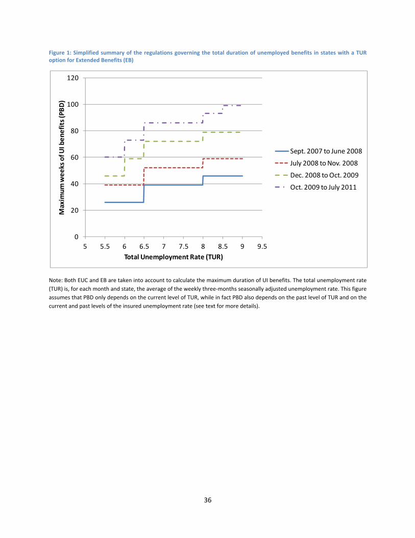
36  

Figure 1: Simplified summary of the regulations governing the total duration of unemployed benefits  in states with a TUR option for Extended Benefits (EB) 

 

Note: Both EUC and EB are taken into account to calculate the maximum duration of UI benefits. The total unemployment rate 

(TUR) is, for each month and state, the average of the weekly three‐months seasonally adjusted unemployment rate. This figure 

assumes that PBD only depends on the current level of TUR, while in fact PBD also depends on the past level of TUR and on the 

current and past levels of the insured unemployment rate (see text for more details).  

   

0

20

40

60

80

100

120

5 5.5 6 6.5 7 7.5 8 8.5 9 9.5

Maxim

um weeks of U

I benefits (PBD)

Total Unemployment Rate (TUR)

Sept. 2007 to June 2008

July 2008 to Nov. 2008

Dec. 2008 to Oct. 2009

Oct. 2009 to July 2011

  

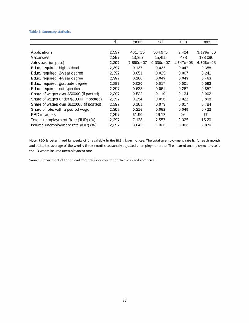
37  

Table 1: Summary statistics 

 

Note: PBD  is determined by weeks of UI available  in the BLS trigger notices. The total unemployment rate  is, for each month 

and state, the average of the weekly three‐months seasonally adjusted unemployment rate. The insured unemployment rate is 

the 13‐weeks insured unemployment rate. 

Source: Department of Labor, and CareerBuilder.com for applications and vacancies. 

   

N mean sd min max

Applications 2,397 431,725 584,975 2,424 3.179e+06Vacancies 2,397 13,357 15,455 438 123,090Job views (snippet) 2,397 7.560e+07 9.336e+07 1.547e+06 6.528e+08Educ. required: high school 2,397 0.137 0.032 0.047 0.358Educ. required: 2-year degree 2,397 0.051 0.025 0.007 0.241Educ. required: 4-year degree 2,397 0.160 0.049 0.043 0.463Educ. required: graduate degree 2,397 0.020 0.017 0.001 0.593Educ. required: not specified 2,397 0.633 0.061 0.267 0.857Share of wages over $50000 (if posted) 2,397 0.522 0.110 0.134 0.902Share of wages under $30000 (if posted) 2,397 0.254 0.096 0.022 0.808Share of wages over $100000 (if posted) 2,397 0.161 0.079 0.017 0.784Share of jobs with a posted wage 2,397 0.216 0.062 0.049 0.433PBD in weeks 2,397 61.90 26.12 26 99Total Unemployment Rate (TUR) (%) 2,397 7.138 2.557 2.325 15.20Insured unemployment rate (IUR) (%) 2,397 3.042 1.326 0.303 7.870

  

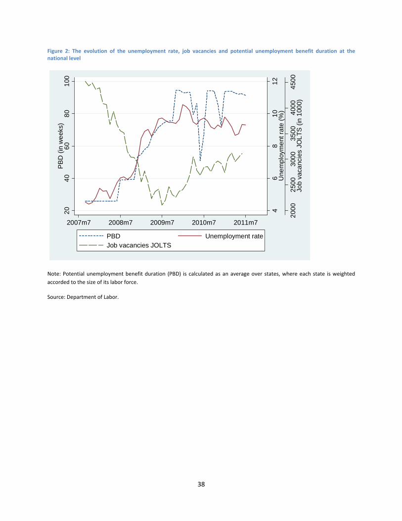
38  

Figure  2:  The  evolution  of  the  unemployment  rate,  job  vacancies  and  potential  unemployment  benefit  duration  at  the national level 

 

Note: Potential unemployment benefit duration  (PBD)  is calculated as an average over states, where each state  is weighted 

accorded to the size of its labor force. 

Source: Department of Labor.   2

000

250

03

000

350

04

000

450

0Jo

b va

canc

ies

JOL

TS

(in

100

0)

46

81

01

2U

nem

ploy

me

nt r

ate

(%

)

20

40

60

80

100

PB

D (

in w

eek

s)

2007m7 2008m7 2009m7 2010m7 2011m7

PBD Unemployment rateJob vacancies JOLTS

  

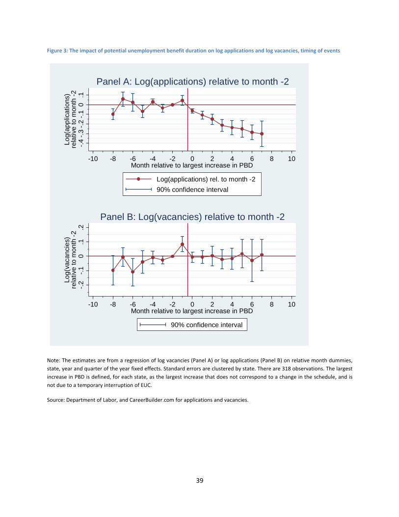
39  

Figure 3: The impact of potential unemployment benefit duration on log applications and log vacancies, timing of events 

 

Note: The estimates are from a regression of log vacancies (Panel A) or log applications (Panel B) on relative month dummies, 

state, year and quarter of the year fixed effects. Standard errors are clustered by state. There are 318 observations. The largest 

increase in PBD is defined, for each state, as the largest increase that does not correspond to a change in the schedule, and is 

not due to a temporary interruption of EUC. 

Source: Department of Labor, and CareerBuilder.com for applications and vacancies. 

   

-.4

-.3

-.2

-.1

0.1

Log(

appl

icat

ions

)re

lativ

e t

o m

onth

-2

-10 -8 -6 -4 -2 0 2 4 6 8 10Month relative to largest increase in PBD

Log(applications) rel. to month -2

90% confidence interval

Panel A: Log(applications) relative to month -2-.

2-.

10

.1.2

Log(

vaca

ncie

s)re

lativ

e to

mon

th -

2

-10 -8 -6 -4 -2 0 2 4 6 8 10Month relative to largest increase in PBD

90% confidence interval

Panel B: Log(vacancies) relative to month -2

  

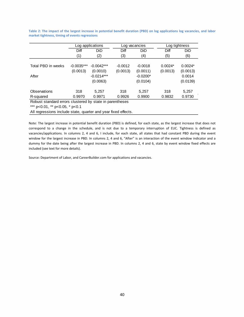
40  

Table 2: The  impact of the  largest  increase  in potential benefit duration (PBD) on  log applications  log vacancies, and  labor market tightness, timing of events regressions 

 

Note: The  largest  increase  in potential benefit duration (PBD)  is defined, for each state, as the  largest  increase that does not 

correspond  to  a  change  in  the  schedule,  and  is  not  due  to  a  temporary  interruption  of  EUC.  Tightness  is  defined  as 

vacancies/applications.  In  columns  2,  4  and  6,  I  include,  for  each  state,  all  states  that  had  constant  PBD  during  the  event 

window  for the  largest  increase  in PBD.  In columns 2, 4 and 6, “After”  is an  interaction of the event window  indicator and a 

dummy  for  the date being after  the  largest  increase  in PBD.  In columns 2, 4 and 6, state by event window  fixed effects are 

included (see text for more details).  

Source: Department of Labor, and CareerBuilder.com for applications and vacancies.   

Diff DiD Diff DiD Diff DiD(1) (2) (3) (4) (5) (6)

Total PBD in weeks -0.0035*** -0.0042*** -0.0012 -0.0018 0.0024* 0.0024*(0.0013) (0.0010) (0.0013) (0.0011) (0.0013) (0.0013)

After -0.0214*** -0.0200* 0.0014(0.0063) (0.0104) (0.0139)

Observations 318 5,257 318 5,257 318 5,257R-squared 0.9970 0.9971 0.9926 0.9900 0.9832 0.9730Robust standard errors clustered by state in parentheses*** p<0.01, ** p<0.05, * p<0.1All regressions include state, quarter and year fixed effects.

Log applications Log vacancies Log tightness

  

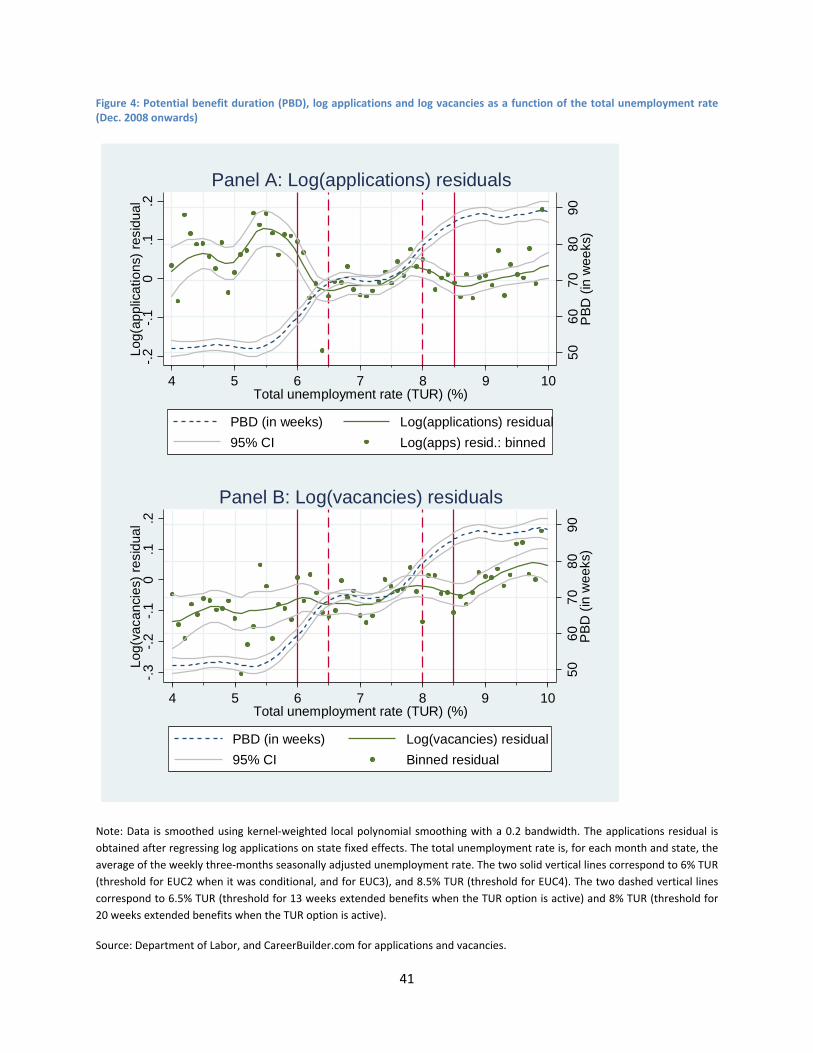
41  

Figure 4: Potential benefit duration (PBD),  log applications and  log vacancies as a function of the total unemployment rate (Dec. 2008 onwards) 

 

Note: Data  is smoothed using kernel‐weighted  local polynomial smoothing with a 0.2 bandwidth. The applications residual  is 

obtained after regressing log applications on state fixed effects. The total unemployment rate is, for each month and state, the 

average of the weekly three‐months seasonally adjusted unemployment rate. The two solid vertical lines correspond to 6% TUR 

(threshold for EUC2 when it was conditional, and for EUC3), and 8.5% TUR (threshold for EUC4). The two dashed vertical lines 

correspond to 6.5% TUR (threshold for 13 weeks extended benefits when the TUR option is active) and 8% TUR (threshold for 

20 weeks extended benefits when the TUR option is active). 

Source: Department of Labor, and CareerBuilder.com for applications and vacancies.   

506

070

8090

PB

D (

in w

eeks

)

-.2

-.1

0.1

.2L

og(a

pplic

atio

ns)

resi

dual

4 5 6 7 8 9 10Total unemployment rate (TUR) (%)

PBD (in weeks) Log(applications) residual

95% CI Log(apps) resid.: binned

Panel A: Log(applications) residuals

5060

708

090

PB

D (

in w

eeks

)

-.3

-.2

-.1

0.1

.2Lo

g(va

canc

ies)

res

idua

l

4 5 6 7 8 9 10Total unemployment rate (TUR) (%)

PBD (in weeks) Log(vacancies) residual

95% CI Binned residual

Panel B: Log(vacancies) residuals

  

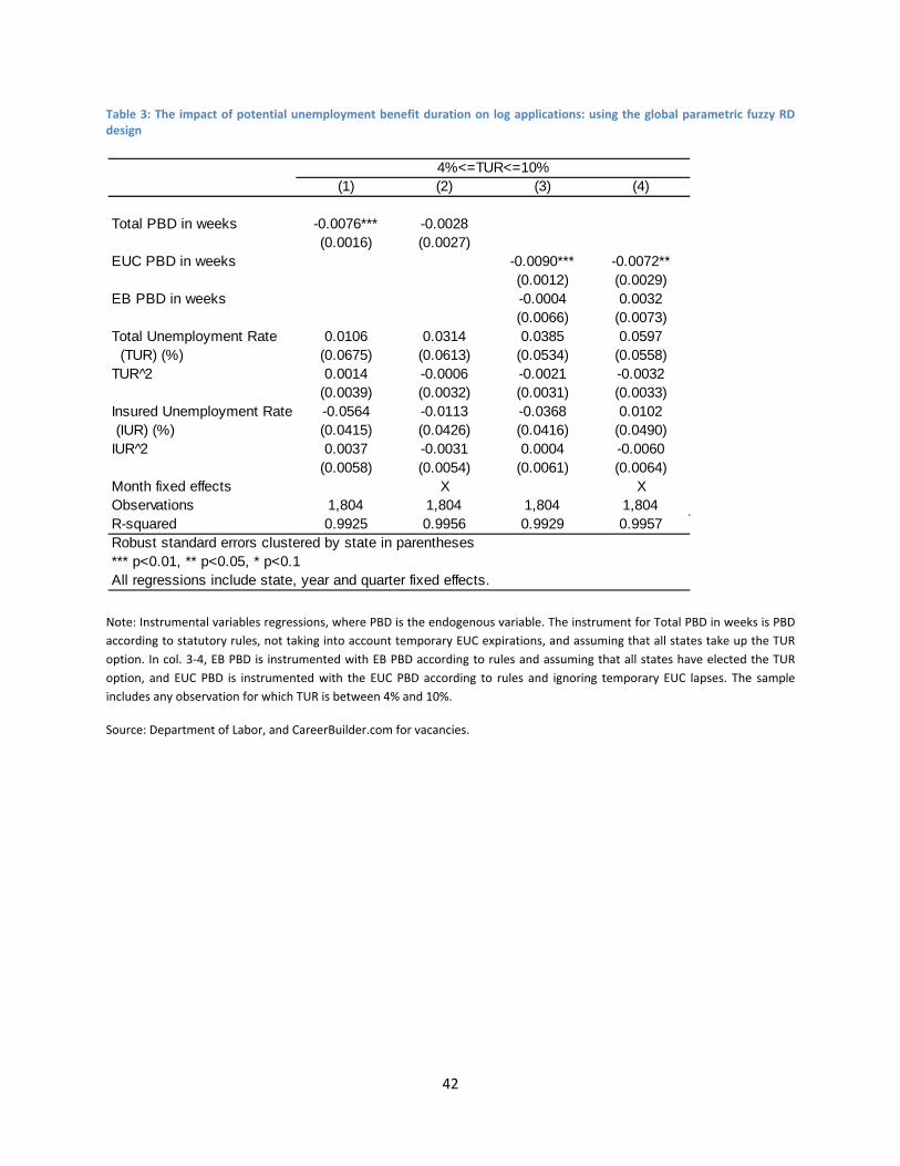
42  

Table 3: The  impact of potential unemployment benefit duration on  log applications: using the global parametric fuzzy RD design 

 

Note: Instrumental variables regressions, where PBD is the endogenous variable. The instrument for Total PBD in weeks is PBD 

according to statutory rules, not taking into account temporary EUC expirations, and assuming that all states take up the TUR 

option.  In col. 3‐4, EB PBD  is  instrumented with EB PBD according to rules and assuming that all states have elected the TUR 

option, and EUC PBD  is  instrumented with  the EUC PBD according  to  rules and  ignoring  temporary EUC  lapses. The  sample 

includes any observation for which TUR is between 4% and 10%.  

Source: Department of Labor, and CareerBuilder.com for vacancies. 

   

(1) (2) (3) (4)

Total PBD in weeks -0.0076*** -0.0028(0.0016) (0.0027)

EUC PBD in weeks -0.0090*** -0.0072**(0.0012) (0.0029)

EB PBD in weeks -0.0004 0.0032(0.0066) (0.0073)

Total Unemployment Rate 0.0106 0.0314 0.0385 0.0597 (TUR) (%) (0.0675) (0.0613) (0.0534) (0.0558)TUR 2̂ 0.0014 -0.0006 -0.0021 -0.0032

(0.0039) (0.0032) (0.0031) (0.0033)Insured Unemployment Rate -0.0564 -0.0113 -0.0368 0.0102 (IUR) (%) (0.0415) (0.0426) (0.0416) (0.0490)IUR 2̂ 0.0037 -0.0031 0.0004 -0.0060

(0.0058) (0.0054) (0.0061) (0.0064)Month fixed effects X XObservations 1,804 1,804 1,804 1,804R-squared 0.9925 0.9956 0.9929 0.9957Robust standard errors clustered by state in parentheses*** p<0.01, ** p<0.05, * p<0.1All regressions include state, year and quarter fixed effects.

4%<=TUR<=10%

  

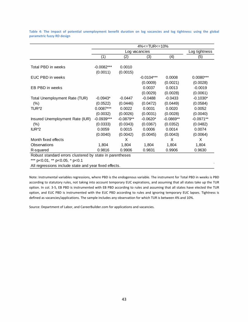
43  

Table  4:  The  impact  of  potential  unemployment  benefit  duration  on  log  vacancies  and  log  tightness:  using  the  global parametric fuzzy RD design 

 

Note: Instrumental variables regressions, where PBD is the endogenous variable. The instrument for Total PBD in weeks is PBD 

according to statutory rules, not taking into account temporary EUC expirations, and assuming that all states take up the TUR 

option.  In col. 3‐5, EB PBD  is  instrumented with EB PBD according to rules and assuming that all states have elected the TUR 

option, and EUC PBD  is  instrumented with  the EUC PBD according  to  rules and  ignoring  temporary EUC  lapses. Tightness  is 

defined as vacancies/applications. The sample includes any observation for which TUR is between 4% and 10%.  

Source: Department of Labor, and CareerBuilder.com for applications and vacancies.   

Log tightness(1) (2) (3) (4) (5)

Total PBD in weeks -0.0082*** 0.0010(0.0011) (0.0015)

EUC PBD in weeks -0.0104*** 0.0008 0.0080***(0.0009) (0.0021) (0.0028)

EB PBD in weeks 0.0037 0.0013 -0.0019(0.0029) (0.0028) (0.0061)

Total Unemployment Rate (TUR) -0.0943* -0.0447 -0.0488 -0.0433 -0.1030* (%) (0.0522) (0.0446) (0.0472) (0.0449) (0.0584)TUR 2̂ 0.0087*** 0.0022 0.0031 0.0020 0.0052

(0.0032) (0.0026) (0.0031) (0.0028) (0.0040)Insured Unemployment Rate (IUR) -0.0939*** -0.0879** -0.0620* -0.0869** -0.0971** (%) (0.0333) (0.0343) (0.0367) (0.0352) (0.0482)IUR 2̂ 0.0059 0.0015 0.0006 0.0014 0.0074

(0.0040) (0.0042) (0.0045) (0.0043) (0.0064)Month fixed effects X X XObservations 1,804 1,804 1,804 1,804 1,804R-squared 0.9816 0.9906 0.9831 0.9906 0.9630Robust standard errors clustered by state in parentheses*** p<0.01, ** p<0.05, * p<0.1All regressions include state and year fixed effects.

Log vacancies4%<=TUR<=10%

  

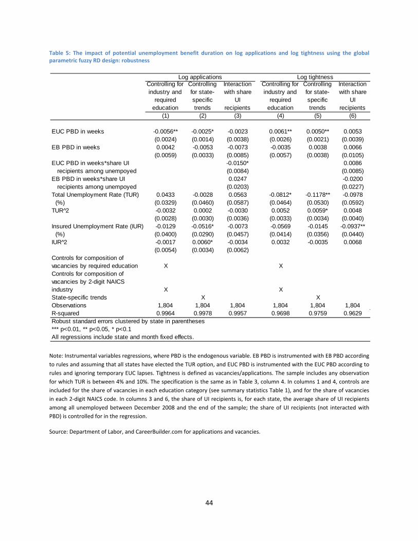
44  

Table  5:  The  impact  of  potential  unemployment  benefit  duration  on  log  applications  and  log  tightness  using  the  global parametric fuzzy RD design: robustness 

 

Note: Instrumental variables regressions, where PBD is the endogenous variable. EB PBD is instrumented with EB PBD according 

to rules and assuming that all states have elected the TUR option, and EUC PBD is instrumented with the EUC PBD according to 

rules and ignoring temporary EUC lapses. Tightness is defined as vacancies/applications. The sample includes any observation 

for which TUR is between 4% and 10%. The specification is the same as in Table 3, column 4. In columns 1 and 4, controls are 

included for the share of vacancies in each education category (see summary statistics Table 1), and for the share of vacancies 

in each 2‐digit NAICS code. In columns 3 and 6, the share of UI recipients is, for each state, the average share of UI recipients 

among all unemployed between December 2008 and  the end of  the sample;  the share of UI  recipients  (not  interacted with 

PBD) is controlled for in the regression.  

Source: Department of Labor, and CareerBuilder.com for applications and vacancies.   

Controlling for industry and

required education

Controlling for state-specific trends

Interaction with share

UI recipients

Controlling for industry and

required education

Controlling for state-specific trends

Interaction with share

UI recipients

(1) (2) (3) (4) (5) (6)

EUC PBD in weeks -0.0056** -0.0025* -0.0023 0.0061** 0.0050** 0.0053(0.0024) (0.0014) (0.0038) (0.0026) (0.0021) (0.0039)

EB PBD in weeks 0.0042 -0.0053 -0.0073 -0.0035 0.0038 0.0066(0.0059) (0.0033) (0.0085) (0.0057) (0.0038) (0.0105)

EUC PBD in weeks*share UI -0.0150* 0.0086recipients among unempoyed (0.0084) (0.0085)

EB PBD in weeks*share UI 0.0247 -0.0200recipients among unempoyed (0.0203) (0.0227)

Total Unemployment Rate (TUR) 0.0433 -0.0028 0.0563 -0.0812* -0.1178** -0.0978 (%) (0.0329) (0.0460) (0.0587) (0.0464) (0.0530) (0.0592)TUR^2 -0.0032 0.0002 -0.0030 0.0052 0.0059* 0.0048

(0.0028) (0.0030) (0.0036) (0.0033) (0.0034) (0.0040)Insured Unemployment Rate (IUR) -0.0129 -0.0516* -0.0073 -0.0569 -0.0145 -0.0937** (%) (0.0400) (0.0290) (0.0457) (0.0414) (0.0356) (0.0440)IUR^2 -0.0017 0.0060* -0.0034 0.0032 -0.0035 0.0068

(0.0054) (0.0034) (0.0062)Controls for composition of vacancies by required education X XControls for composition of vacancies by 2-digit NAICS industry X XState-specific trends X XObservations 1,804 1,804 1,804 1,804 1,804 1,804R-squared 0.9964 0.9978 0.9957 0.9698 0.9759 0.9629Robust standard errors clustered by state in parentheses*** p<0.01, ** p<0.05, * p<0.1All regressions include state and month fixed effects.

Log applications Log tightness

 

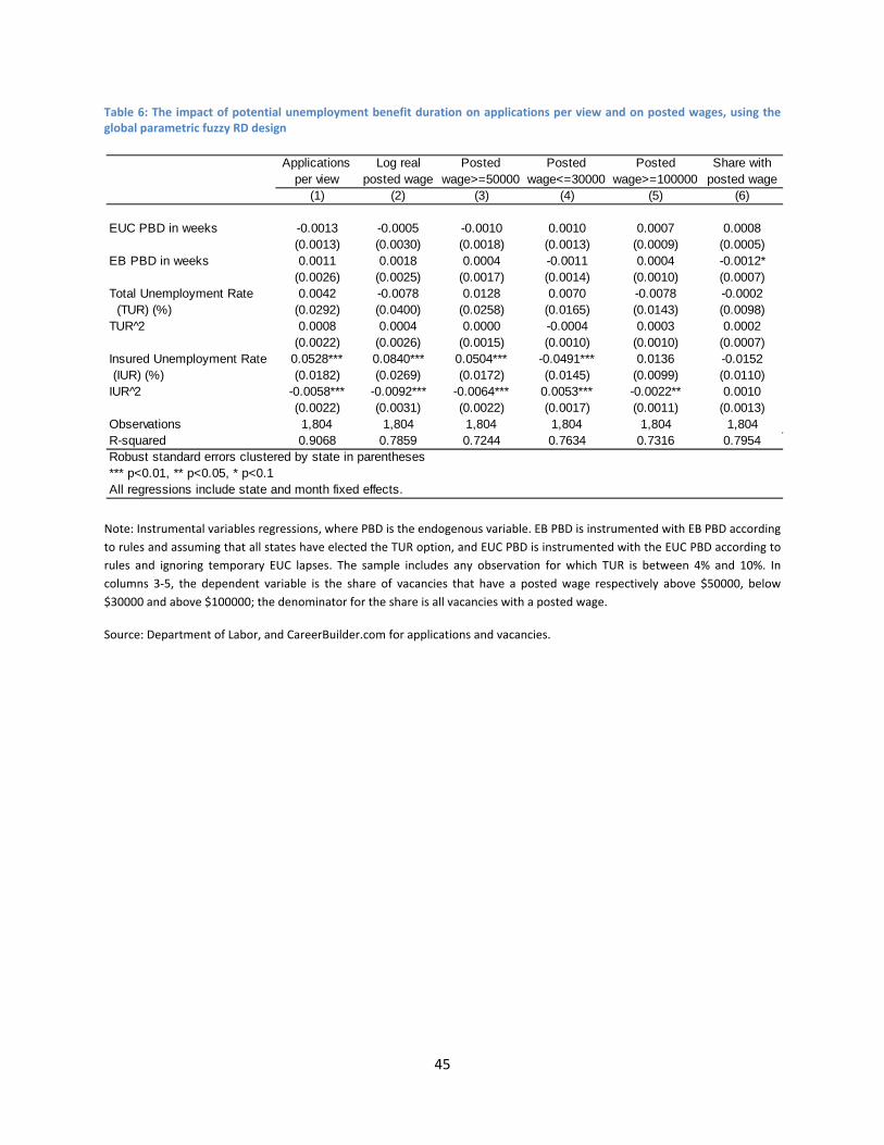
45  

Table 6: The  impact of potential unemployment benefit duration on applications per view and on posted wages, using the global parametric fuzzy RD design 

 

Note: Instrumental variables regressions, where PBD is the endogenous variable. EB PBD is instrumented with EB PBD according 

to rules and assuming that all states have elected the TUR option, and EUC PBD is instrumented with the EUC PBD according to 

rules  and  ignoring  temporary  EUC  lapses.  The  sample  includes  any  observation  for which  TUR  is  between  4%  and  10%.  In 

columns  3‐5,  the dependent  variable  is  the  share of  vacancies  that have  a posted wage  respectively  above  $50000, below 

$30000 and above $100000; the denominator for the share is all vacancies with a posted wage. 

Source: Department of Labor, and CareerBuilder.com for applications and vacancies. 

Applications per view

Log real posted wage

Posted wage>=50000

Posted wage<=30000

Posted wage>=100000

Share with posted wage

(1) (2) (3) (4) (5) (6)

EUC PBD in weeks -0.0013 -0.0005 -0.0010 0.0010 0.0007 0.0008(0.0013) (0.0030) (0.0018) (0.0013) (0.0009) (0.0005)

EB PBD in weeks 0.0011 0.0018 0.0004 -0.0011 0.0004 -0.0012*(0.0026) (0.0025) (0.0017) (0.0014) (0.0010) (0.0007)

Total Unemployment Rate 0.0042 -0.0078 0.0128 0.0070 -0.0078 -0.0002 (TUR) (%) (0.0292) (0.0400) (0.0258) (0.0165) (0.0143) (0.0098)TUR^2 0.0008 0.0004 0.0000 -0.0004 0.0003 0.0002

(0.0022) (0.0026) (0.0015) (0.0010) (0.0010) (0.0007)Insured Unemployment Rate 0.0528*** 0.0840*** 0.0504*** -0.0491*** 0.0136 -0.0152 (IUR) (%) (0.0182) (0.0269) (0.0172) (0.0145) (0.0099) (0.0110)IUR 2̂ -0.0058*** -0.0092*** -0.0064*** 0.0053*** -0.0022** 0.0010

(0.0022) (0.0031) (0.0022) (0.0017) (0.0011) (0.0013)Observations 1,804 1,804 1,804 1,804 1,804 1,804R-squared 0.9068 0.7859 0.7244 0.7634 0.7316 0.7954Robust standard errors clustered by state in parentheses*** p<0.01, ** p<0.05, * p<0.1All regressions include state and month fixed effects.

 

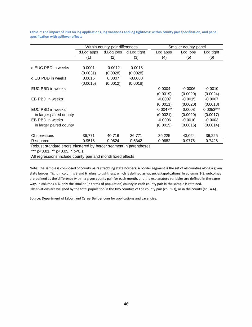
46  

Table 7: The impact of PBD on log applications, log vacancies and log tightness: within county pair specification, and panel specification with spillover effects 

 

Note: The sample is composed of county pairs straddling state borders. A border segment is the set of all counties along a given 

state border. Tight in columns 3 and 6 refers to tightness, which is defined as vacancies/applications. In columns 1‐3, outcomes 

are defined as the difference within a given county pair for each month, and the explanatory variables are defined in the same 

way. In columns 4‐6, only the smaller (in terms of population) county in each county pair in the sample is retained. 

Observations are weighed by the total population in the two counties of the county pair (col. 1‐3), or in the county (col. 4‐6). 

Source: Department of Labor, and CareerBuilder.com for applications and vacancies.

d.Log apps d.Log jobs d.Log tight Log apps Log jobs Log tight(1) (2) (3) (4) (5) (6)

d.EUC PBD in weeks 0.0001 -0.0012 -0.0016(0.0031) (0.0028) (0.0028)

d.EB PBD in weeks 0.0016 0.0007 -0.0008(0.0015) (0.0012) (0.0018)

EUC PBD in weeks 0.0004 -0.0006 -0.0010(0.0019) (0.0020) (0.0024)

EB PBD in weeks -0.0007 -0.0015 -0.0007(0.0011) (0.0020) (0.0018)

EUC PBD in weeks -0.0047** 0.0003 0.0053***in larger paired county (0.0021) (0.0020) (0.0017)

EB PBD in weeks -0.0006 -0.0010 -0.0003in larger paired county (0.0015) (0.0016) (0.0014)

Observations 36,771 40,716 36,771 39,225 43,024 39,225R-squared 0.9516 0.9624 0.6342 0.9682 0.9776 0.7426Robust standard errors clustered by border segment in parentheses*** p<0.01, ** p<0.05, * p<0.1All regressions include county pair and month fixed effects.

Within county pair differences Smaller county panel

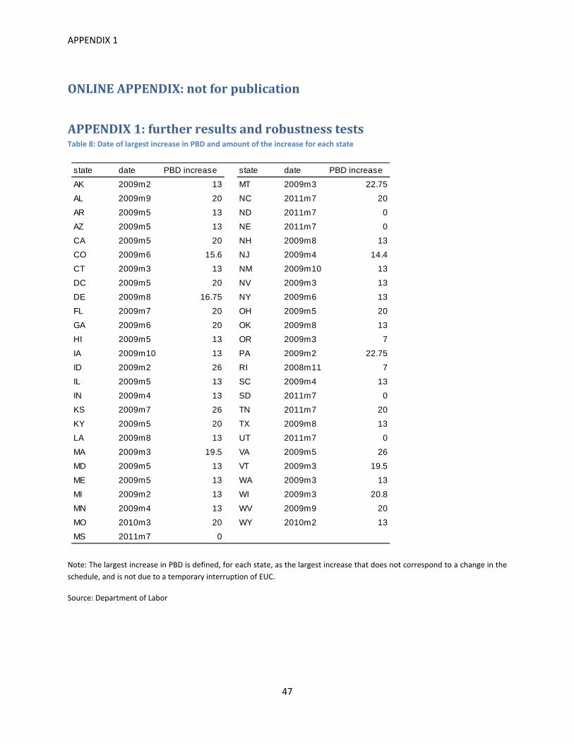
APPENDIX 1 

47  

ONLINEAPPENDIX:notforpublication

APPENDIX1:furtherresultsandrobustnesstestsTable 8: Date of largest increase in PBD and amount of the increase for each state 

    

Note: The largest increase in PBD is defined, for each state, as the largest increase that does not correspond to a change in the 

schedule, and is not due to a temporary interruption of EUC. 

Source: Department of Labor   

state date PBD increase state date PBD increase

AK 2009m2 13 MT 2009m3 22.75

AL 2009m9 20 NC 2011m7 20

AR 2009m5 13 ND 2011m7 0

AZ 2009m5 13 NE 2011m7 0

CA 2009m5 20 NH 2009m8 13

CO 2009m6 15.6 NJ 2009m4 14.4

CT 2009m3 13 NM 2009m10 13

DC 2009m5 20 NV 2009m3 13

DE 2009m8 16.75 NY 2009m6 13

FL 2009m7 20 OH 2009m5 20

GA 2009m6 20 OK 2009m8 13

HI 2009m5 13 OR 2009m3 7

IA 2009m10 13 PA 2009m2 22.75

ID 2009m2 26 RI 2008m11 7

IL 2009m5 13 SC 2009m4 13

IN 2009m4 13 SD 2011m7 0

KS 2009m7 26 TN 2011m7 20

KY 2009m5 20 TX 2009m8 13

LA 2009m8 13 UT 2011m7 0

MA 2009m3 19.5 VA 2009m5 26

MD 2009m5 13 VT 2009m3 19.5

ME 2009m5 13 WA 2009m3 13

MI 2009m2 13 WI 2009m3 20.8

MN 2009m4 13 WV 2009m9 20

MO 2010m3 20 WY 2010m2 13

MS 2011m7 0

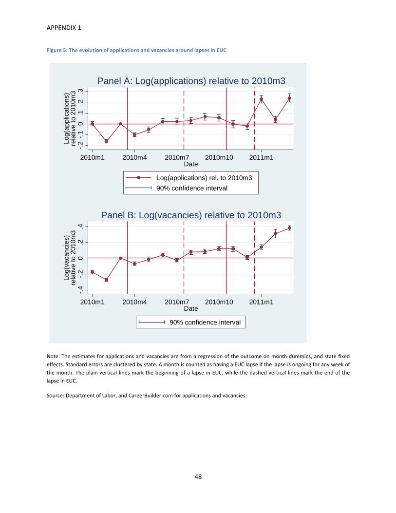
APPENDIX 1 

48  

Figure 5: The evolution of applications and vacancies around lapses in EUC 

 

Note: The estimates for applications and vacancies are from a regression of the outcome on month dummies, and state fixed 

effects. Standard errors are clustered by state. A month is counted as having a EUC lapse if the lapse is ongoing for any week of 

the month. The plain vertical  lines mark the beginning of a  lapse  in EUC, while the dashed vertical  lines mark the end of the 

lapse in EUC. 

Source: Department of Labor, and CareerBuilder.com for applications and vacancies. 

   

-.2

-.1

0.1

.2.3

Log(

appl

icat

ions

)re

lativ

e to

201

0m3

2010m1 2010m4 2010m7 2010m10 2011m1Date

Log(applications) rel. to 2010m3

90% confidence interval

Panel A: Log(applications) relative to 2010m3-.

4-.

20

.2.4

Log(

vaca

ncie

s)re

lativ

e to

201

0m3

2010m1 2010m4 2010m7 2010m10 2011m1Date

90% confidence interval

Panel B: Log(vacancies) relative to 2010m3

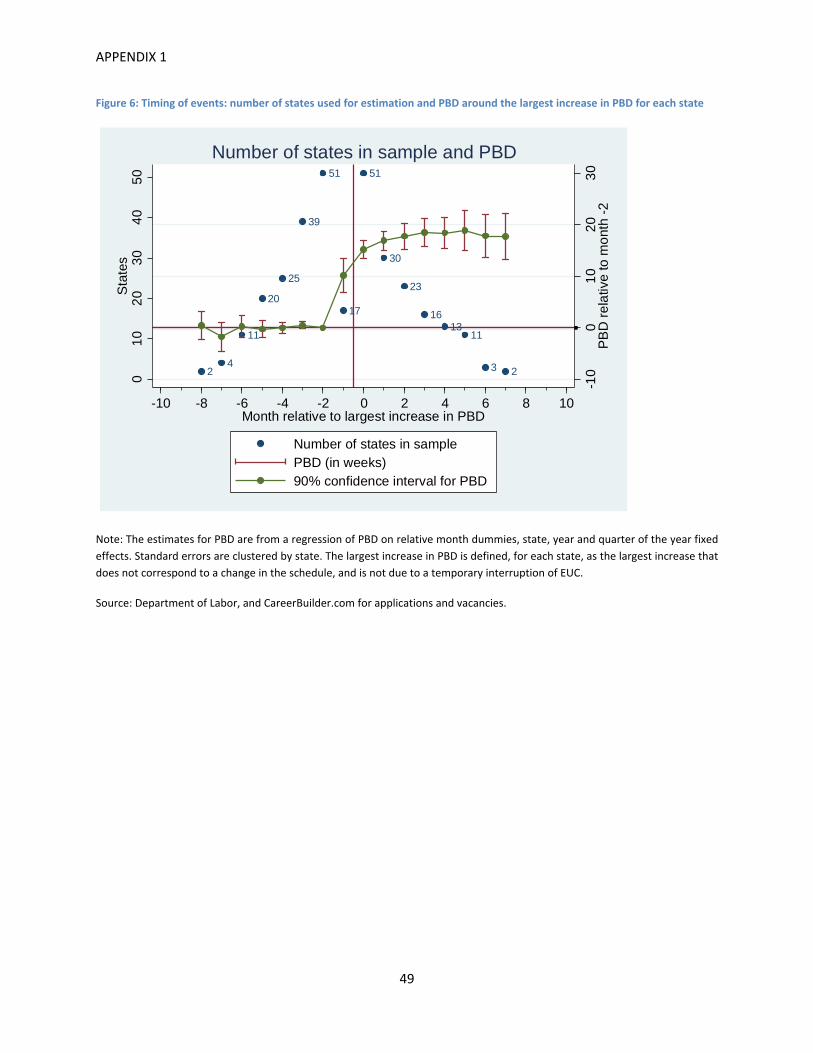
APPENDIX 1 

49  

Figure 6: Timing of events: number of states used for estimation and PBD around the largest increase in PBD for each state 

 

Note: The estimates for PBD are from a regression of PBD on relative month dummies, state, year and quarter of the year fixed 

effects. Standard errors are clustered by state. The largest increase in PBD is defined, for each state, as the largest increase that 

does not correspond to a change in the schedule, and is not due to a temporary interruption of EUC. 

Source: Department of Labor, and CareerBuilder.com for applications and vacancies. 

 

24

11

20

25

39

51

17

51

30

23

1613

11

3 2

-10

01

02

03

0P

BD

re

lativ

e to

mo

nth

-2

01

02

03

04

05

0S

tate

s

-10 -8 -6 -4 -2 0 2 4 6 8 10Month relative to largest increase in PBD

Number of states in samplePBD (in weeks)90% confidence interval for PBD

Number of states in sample and PBD

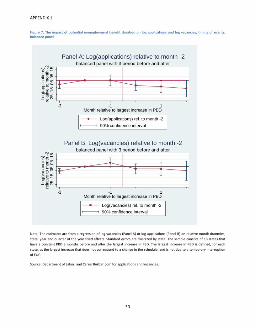
APPENDIX 1 

50  

Figure 7: The  impact of potential unemployment benefit duration on  log applications and  log vacancies,  timing of events, balanced panel 

 

Note: The estimates are from a regression of log vacancies (Panel A) or log applications (Panel B) on relative month dummies, 

state, year and quarter of the year fixed effects. Standard errors are clustered by state. The sample consists of 18 states that 

have a constant PBD 3 months before and after  the  largest  increase  in PBD. The  largest  increase  in PBD  is defined,  for each 

state, as the largest increase that does not correspond to a change in the schedule, and is not due to a temporary interruption 

of EUC. 

Source: Department of Labor, and CareerBuilder.com for applications and vacancies. 

-.25

-.15

-.05

.05

.15

Log(

appl

icat

ions

)re

lativ

e t

o m

onth

-2

-3 -1 1Month relative to largest increase in PBD

Log(applications) rel. to month -2

90% confidence interval

balanced panel with 3 period before and afterPanel A: Log(applications) relative to month -2

-.25

-.15

-.05

.05

.15

Log(

vaca

ncie

s)re

lativ

e to

mon

th -

2

-3 -1 1Month relative to largest increase in PBD

Log(vacancies) rel. to month -2

90% confidence interval

balanced panel with 3 period before and afterPanel B: Log(vacancies) relative to month -2

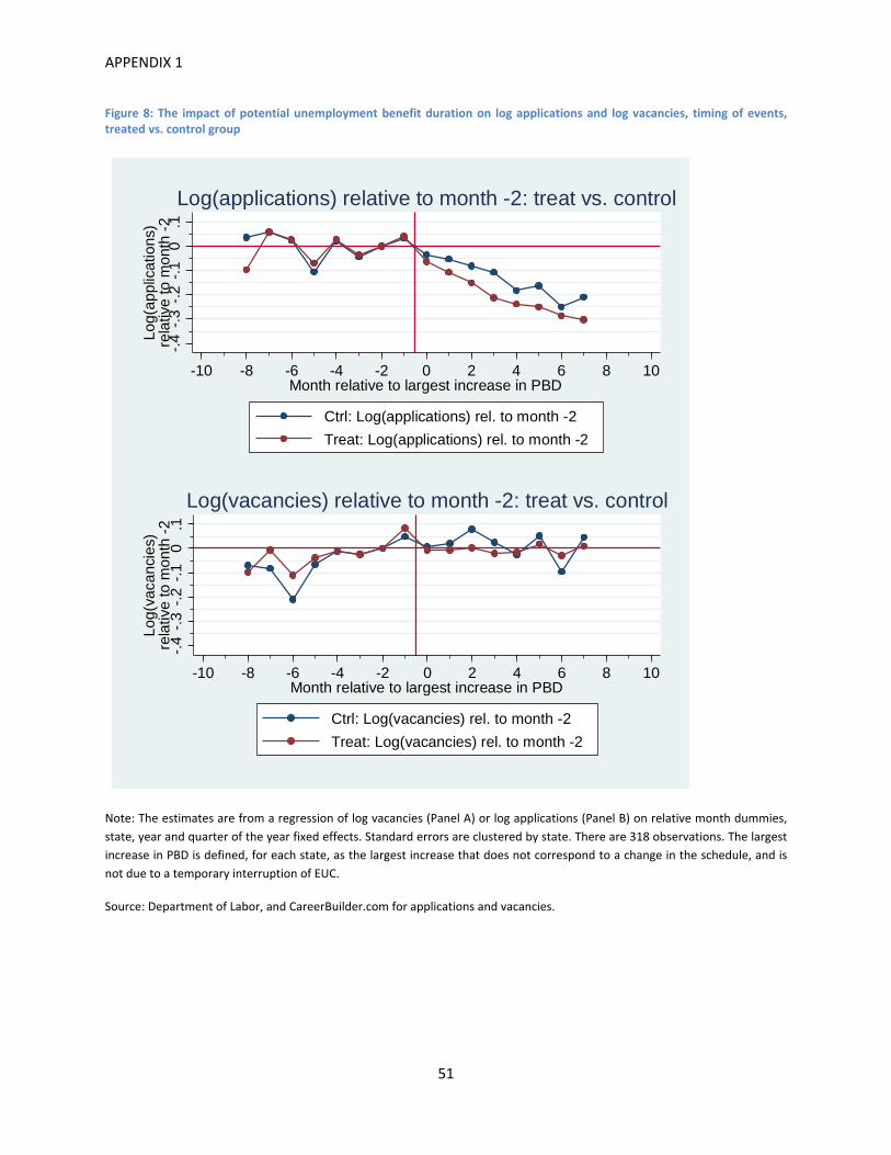
APPENDIX 1 

51  

Figure 8: The  impact of potential unemployment benefit duration on  log applications and  log vacancies,  timing of events, treated vs. control group 

 

Note: The estimates are from a regression of log vacancies (Panel A) or log applications (Panel B) on relative month dummies, 

state, year and quarter of the year fixed effects. Standard errors are clustered by state. There are 318 observations. The largest 

increase in PBD is defined, for each state, as the largest increase that does not correspond to a change in the schedule, and is 

not due to a temporary interruption of EUC. 

Source: Department of Labor, and CareerBuilder.com for applications and vacancies. 

   

-.4

-.3

-.2

-.1

0.1

Log(

appl

icat

ions

)re

lativ

e t

o m

onth

-2

-10 -8 -6 -4 -2 0 2 4 6 8 10Month relative to largest increase in PBD

Ctrl: Log(applications) rel. to month -2

Treat: Log(applications) rel. to month -2

Log(applications) relative to month -2: treat vs. control-.

4-.

3-.

2-.

10

.1

Log(

vaca

ncie

s)re

lativ

e to

mon

th -

2

-10 -8 -6 -4 -2 0 2 4 6 8 10Month relative to largest increase in PBD

Ctrl: Log(vacancies) rel. to month -2

Treat: Log(vacancies) rel. to month -2

Log(vacancies) relative to month -2: treat vs. control

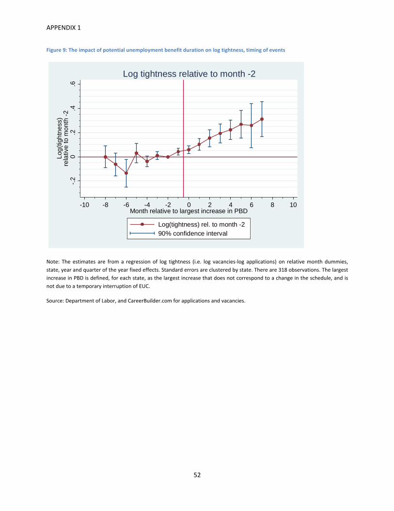
APPENDIX 1 

52  

Figure 9: The impact of potential unemployment benefit duration on log tightness, timing of events 

 

Note: The estimates are  from a  regression of  log  tightness  (i.e.  log  vacancies‐log applications) on  relative month dummies, 

state, year and quarter of the year fixed effects. Standard errors are clustered by state. There are 318 observations. The largest 

increase in PBD is defined, for each state, as the largest increase that does not correspond to a change in the schedule, and is 

not due to a temporary interruption of EUC. 

Source: Department of Labor, and CareerBuilder.com for applications and vacancies. 

   

-.2

0.2

.4.6

Log

(tig

htn

ess)

rela

tive

to m

ont

h -2

-10 -8 -6 -4 -2 0 2 4 6 8 10Month relative to largest increase in PBD

Log(tightness) rel. to month -290% confidence interval

Log tightness relative to month -2

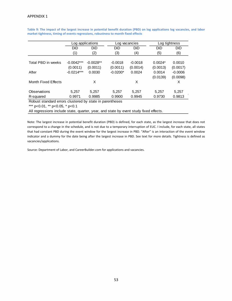
APPENDIX 1 

53  

Table 9: The  impact of the  largest  increase  in potential benefit duration (PBD) on  log applications  log vacancies, and  labor market tightness, timing of events regressions, robustness to month fixed effects 

 

Note: The  largest  increase  in potential benefit duration (PBD)  is defined, for each state, as the  largest  increase that does not 

correspond to a change in the schedule, and is not due to a temporary interruption of EUC. I include, for each state, all states 

that had constant PBD during the event window for the largest increase in PBD. “After” is an interaction of the event window 

indicator and a dummy for the date being after the  largest  increase  in PBD. See text for more details. Tightness  is defined as 

vacancies/applications. 

Source: Department of Labor, and CareerBuilder.com for applications and vacancies. 

   

DiD DiD DiD DiD DiD DiD(1) (2) (3) (4) (5) (6)

Total PBD in weeks -0.0042*** -0.0028** -0.0018 -0.0018 0.0024* 0.0010(0.0011) (0.0011) (0.0011) (0.0014) (0.0013) (0.0017)

After -0.0214*** 0.0030 -0.0200* 0.0024 0.0014 -0.0006(0.0139) (0.0098)

Month Fixed Effects X X X

Observations 5,257 5,257 5,257 5,257 5,257 5,257R-squared 0.9971 0.9985 0.9900 0.9945 0.9730 0.9813Robust standard errors clustered by state in parentheses*** p<0.01, ** p<0.05, * p<0.1All regressions include state, quarter, year, and state by event study fixed effects.

Log applications Log vacancies Log tightness

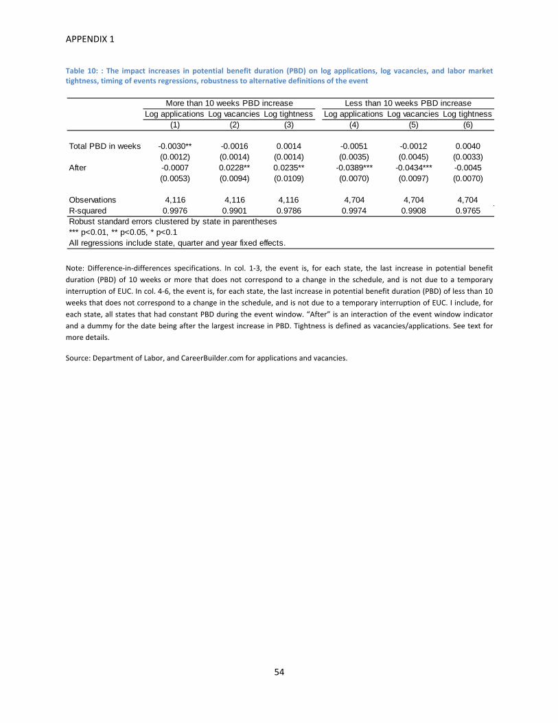
APPENDIX 1 

54  

Table 10:  : The  impact  increases  in potential benefit duration  (PBD) on  log applications,  log vacancies, and  labor market tightness, timing of events regressions, robustness to alternative definitions of the event 

 

Note: Difference‐in‐differences  specifications.  In  col.  1‐3,  the  event  is,  for  each  state,  the  last  increase  in  potential  benefit 

duration  (PBD) of 10 weeks or more  that does not  correspond  to a  change  in  the  schedule, and  is not due  to a  temporary 

interruption of EUC. In col. 4‐6, the event is, for each state, the last increase in potential benefit duration (PBD) of less than 10 

weeks that does not correspond to a change in the schedule, and is not due to a temporary interruption of EUC. I include, for 

each state, all states that had constant PBD during the event window. “After” is an interaction of the event window indicator 

and a dummy for the date being after the  largest  increase  in PBD. Tightness  is defined as vacancies/applications. See text for 

more details. 

Source: Department of Labor, and CareerBuilder.com for applications and vacancies. 

   

Log applications Log vacancies Log tightness Log applications Log vacancies Log tightness(1) (2) (3) (4) (5) (6)

Total PBD in weeks -0.0030** -0.0016 0.0014 -0.0051 -0.0012 0.0040(0.0012) (0.0014) (0.0014) (0.0035) (0.0045) (0.0033)

After -0.0007 0.0228** 0.0235** -0.0389*** -0.0434*** -0.0045(0.0053) (0.0094) (0.0109) (0.0070) (0.0097) (0.0070)

Observations 4,116 4,116 4,116 4,704 4,704 4,704R-squared 0.9976 0.9901 0.9786 0.9974 0.9908 0.9765Robust standard errors clustered by state in parentheses*** p<0.01, ** p<0.05, * p<0.1All regressions include state, quarter and year fixed effects.

More than 10 weeks PBD increase Less than 10 weeks PBD increase

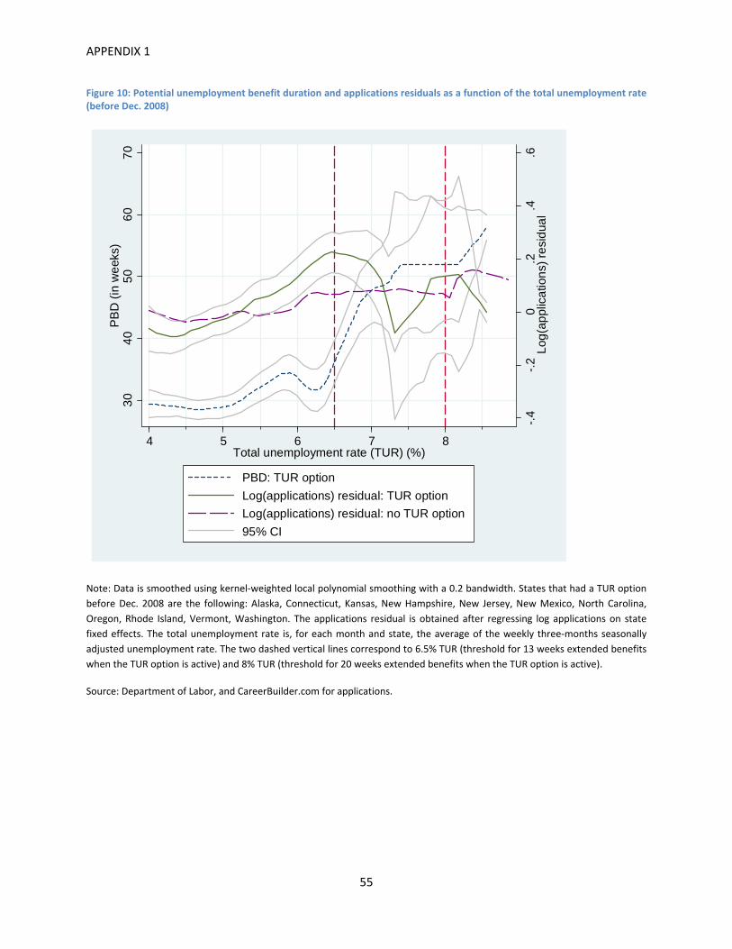
APPENDIX 1 

55  

Figure 10: Potential unemployment benefit duration and applications residuals as a function of the total unemployment rate (before Dec. 2008) 

 

Note: Data is smoothed using kernel‐weighted local polynomial smoothing with a 0.2 bandwidth. States that had a TUR option 

before Dec. 2008 are  the  following: Alaska, Connecticut, Kansas, New Hampshire, New  Jersey, New Mexico, North Carolina, 

Oregon, Rhode  Island, Vermont, Washington. The applications  residual  is obtained after  regressing  log applications on  state 

fixed effects. The total unemployment rate  is,  for each month and state, the average of the weekly three‐months seasonally 

adjusted unemployment rate. The two dashed vertical lines correspond to 6.5% TUR (threshold for 13 weeks extended benefits 

when the TUR option is active) and 8% TUR (threshold for 20 weeks extended benefits when the TUR option is active). 

Source: Department of Labor, and CareerBuilder.com for applications.  

-.4

-.2

0.2

.4.6

Log

(ap

plic

atio

ns)

re

sid

ual

30

40

50

60

70

PB

D (

in w

eek

s)

4 5 6 7 8Total unemployment rate (TUR) (%)

PBD: TUR option

Log(applications) residual: TUR option

Log(applications) residual: no TUR option

95% CI

APPENDIX 1 

56  

Figure 11: Potential unemployment benefit duration and applications residuals as a function of the insured unemployment rate (Dec. 2008 onwards) 

 

Note: Data  is smoothed using kernel‐weighted  local polynomial smoothing with a 0.2 bandwidth. The applications residual  is 

obtained after regressing log applications on state fixed effects. The two solid vertical lines correspond to 4% IUR (threshold for 

EUC), and 6% IUR (threshold for EUC). The dashed vertical line corresponds to 5% IUR (threshold for EB). In Panel B, the data is 

restricted to monthly TUR<6% so that TUR conditions are unlikely to trigger higher PBD. 

Source: Department of Labor, and CareerBuilder.com for applications and vacancies. 

-.2

-.1

0.1

Lo

g(a

pp

lica

tion

s) r

esi

du

al

60

70

80

90

PB

D (

in w

eeks

)

2 3 4 5 6 7 8Insured unemployment rate (IUR) (%)

PBD (in weeks) Log(applications) residual

95% CI

Panel A: Log(applications) residuals

-.1

0.1

.2.3

Lo

g(a

pp

lica

tion

s) r

esi

du

al

40

50

60

70

80

PB

D (

in w

eeks

)

2 3 4 5 6 7 8Insured unemployment rate (IUR) (%)

PBD (in weeks) Log(applications) residual

95% CI

Panel B: Log(applications) residuals, TUR<6%

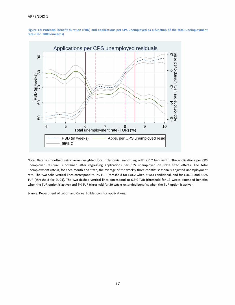
APPENDIX 1 

57  

Figure 12: Potential benefit duration (PBD) and applications per CPS unemployed as a function of the total unemployment rate (Dec. 2008 onwards) 

 

Note: Data  is  smoothed using  kernel‐weighted  local polynomial  smoothing with  a  0.2 bandwidth.  The  applications per CPS 

unemployed  residual  is  obtained  after  regressing  applications  per  CPS  unemployed  on  state  fixed  effects.  The  total 

unemployment rate is, for each month and state, the average of the weekly three‐months seasonally adjusted unemployment 

rate. The two solid vertical lines correspond to 6% TUR (threshold for EUC2 when it was conditional, and for EUC3), and 8.5% 

TUR  (threshold  for EUC4). The  two dashed vertical  lines correspond  to 6.5% TUR  (threshold  for 13 weeks extended benefits 

when the TUR option is active) and 8% TUR (threshold for 20 weeks extended benefits when the TUR option is active). 

Source: Department of Labor, and CareerBuilder.com for applications. 

-.6

-.4

-.2

0.2

Ap

plic

atio

ns

per

CP

S u

nem

plo

yed

re

sid

.

50

60

70

80

90

PB

D (

in w

eek

s)

4 5 6 7 8 9 10Total unemployment rate (TUR) (%)

PBD (in weeks) Apps. per CPS unemployed resid.95% CI

Applications per CPS unemployed residuals

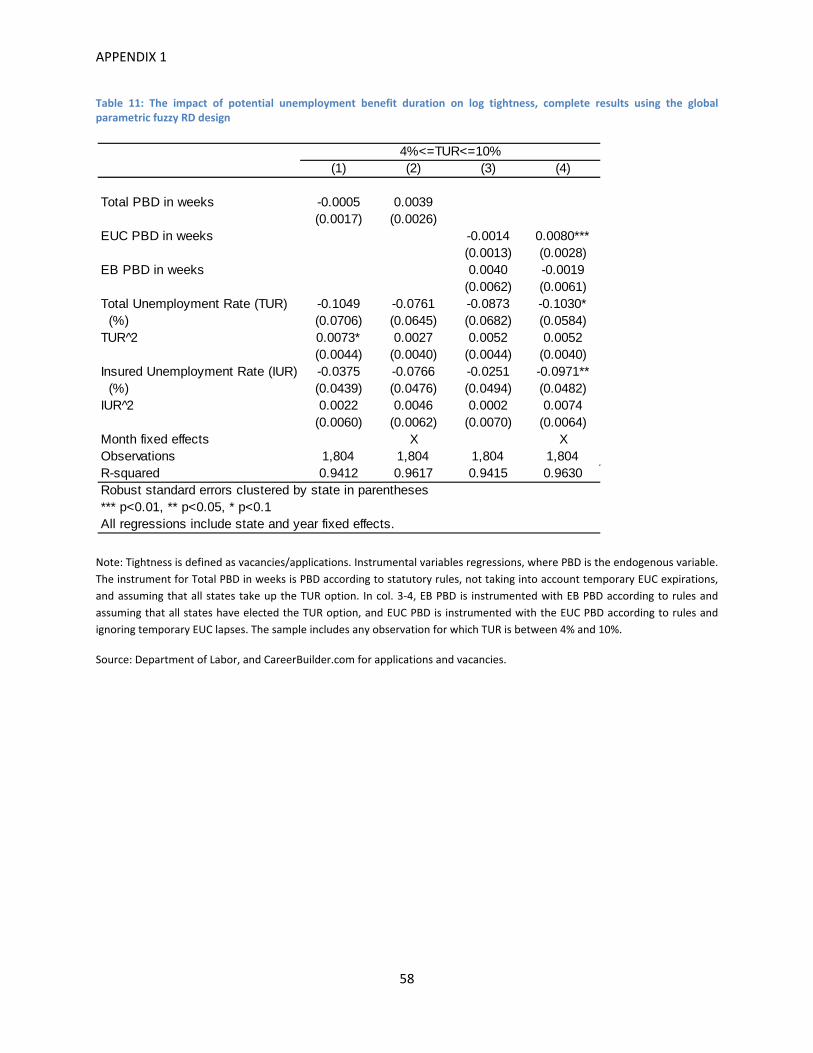
APPENDIX 1 

58  

Table  11:  The  impact  of  potential  unemployment  benefit  duration  on  log  tightness,  complete  results  using  the  global parametric fuzzy RD design 

 

Note: Tightness is defined as vacancies/applications. Instrumental variables regressions, where PBD is the endogenous variable. 

The instrument for Total PBD in weeks is PBD according to statutory rules, not taking into account temporary EUC expirations, 

and assuming that all states take up the TUR option.  In col. 3‐4, EB PBD  is  instrumented with EB PBD according to rules and 

assuming that all states have elected the TUR option, and EUC PBD  is  instrumented with the EUC PBD according to rules and 

ignoring temporary EUC lapses. The sample includes any observation for which TUR is between 4% and 10%.  

Source: Department of Labor, and CareerBuilder.com for applications and vacancies. 

(1) (2) (3) (4)

Total PBD in weeks -0.0005 0.0039(0.0017) (0.0026)

EUC PBD in weeks -0.0014 0.0080***(0.0013) (0.0028)

EB PBD in weeks 0.0040 -0.0019(0.0062) (0.0061)

Total Unemployment Rate (TUR) -0.1049 -0.0761 -0.0873 -0.1030* (%) (0.0706) (0.0645) (0.0682) (0.0584)TUR 2̂ 0.0073* 0.0027 0.0052 0.0052

(0.0044) (0.0040) (0.0044) (0.0040)Insured Unemployment Rate (IUR) -0.0375 -0.0766 -0.0251 -0.0971** (%) (0.0439) (0.0476) (0.0494) (0.0482)IUR 2̂ 0.0022 0.0046 0.0002 0.0074

(0.0060) (0.0062) (0.0070) (0.0064)Month fixed effects X XObservations 1,804 1,804 1,804 1,804R-squared 0.9412 0.9617 0.9415 0.9630Robust standard errors clustered by state in parentheses*** p<0.01, ** p<0.05, * p<0.1All regressions include state and year fixed effects.

4%<=TUR<=10%

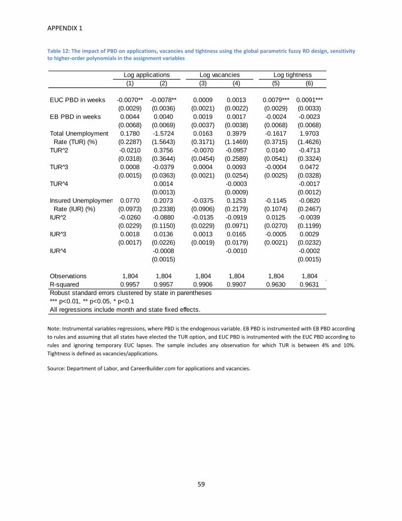
APPENDIX 1 

59  

Table 12: The impact of PBD on applications, vacancies and tightness using the global parametric fuzzy RD design, sensitivity to higher‐order polynomials in the assignment variables 

  

Note: Instrumental variables regressions, where PBD is the endogenous variable. EB PBD is instrumented with EB PBD according 

to rules and assuming that all states have elected the TUR option, and EUC PBD is instrumented with the EUC PBD according to 

rules  and  ignoring  temporary  EUC  lapses.  The  sample  includes  any  observation  for  which  TUR  is  between  4%  and  10%. 

Tightness is defined as vacancies/applications. 

Source: Department of Labor, and CareerBuilder.com for applications and vacancies. 

(1) (2) (3) (4) (5) (6)

EUC PBD in weeks -0.0070** -0.0078** 0.0009 0.0013 0.0079*** 0.0091***(0.0029) (0.0036) (0.0021) (0.0022) (0.0029) (0.0033)

EB PBD in weeks 0.0044 0.0040 0.0019 0.0017 -0.0024 -0.0023(0.0068) (0.0069) (0.0037) (0.0038) (0.0068) (0.0068)

Total Unemployment 0.1780 -1.5724 0.0163 0.3979 -0.1617 1.9703 Rate (TUR) (%) (0.2287) (1.5643) (0.3171) (1.1469) (0.3715) (1.4626)TUR 2̂ -0.0210 0.3756 -0.0070 -0.0957 0.0140 -0.4713

(0.0318) (0.3644) (0.0454) (0.2589) (0.0541) (0.3324)TUR 3̂ 0.0008 -0.0379 0.0004 0.0093 -0.0004 0.0472

(0.0015) (0.0363) (0.0021) (0.0254) (0.0025) (0.0328)TUR 4̂ 0.0014 -0.0003 -0.0017

(0.0013) (0.0009) (0.0012)Insured Unemploymen 0.0770 0.2073 -0.0375 0.1253 -0.1145 -0.0820 Rate (IUR) (%) (0.0973) (0.2338) (0.0906) (0.2179) (0.1074) (0.2467)IUR 2̂ -0.0260 -0.0880 -0.0135 -0.0919 0.0125 -0.0039

(0.0229) (0.1150) (0.0229) (0.0971) (0.0270) (0.1199)IUR 3̂ 0.0018 0.0136 0.0013 0.0165 -0.0005 0.0029

(0.0017) (0.0226) (0.0019) (0.0179) (0.0021) (0.0232)IUR 4̂ -0.0008 -0.0010 -0.0002

(0.0015) (0.0015)

Observations 1,804 1,804 1,804 1,804 1,804 1,804R-squared 0.9957 0.9957 0.9906 0.9907 0.9630 0.9631Robust standard errors clustered by state in parentheses*** p<0.01, ** p<0.05, * p<0.1All regressions include month and state fixed effects.

Log applications Log vacancies Log tightness

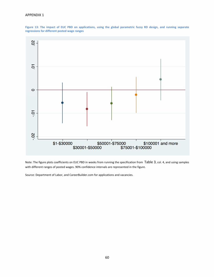
APPENDIX 1 

60  

Figure  13:  The  impact  of  EUC  PBD  on  applications,  using  the  global  parametric  fuzzy  RD  design,  and  running  separate regressions for different posted wage ranges 

 

Note: The figure plots coefficients on EUC PBD in weeks from running the specification from  Table 3, col. 4, and using samples 

with different ranges of posted wages. 90% confidence intervals are represented in the figure. 

Source: Department of Labor, and CareerBuilder.com for applications and vacancies. 

   

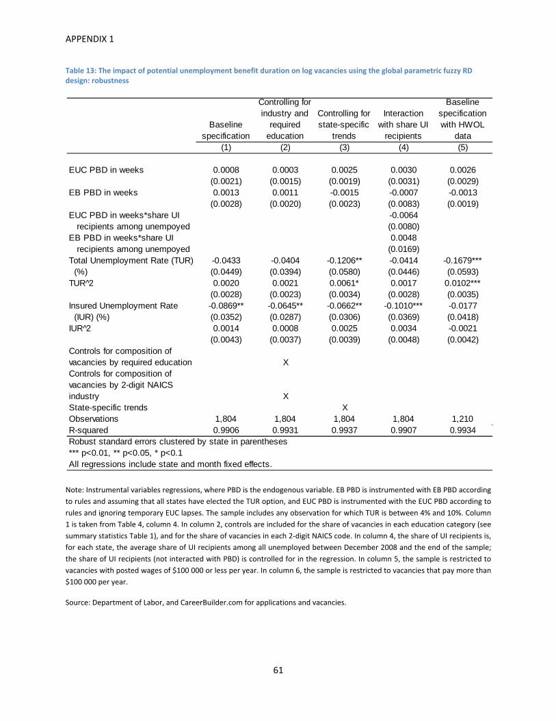
APPENDIX 1 

61  

Table 13: The impact of potential unemployment benefit duration on log vacancies using the global parametric fuzzy RD design: robustness 

 

Note: Instrumental variables regressions, where PBD is the endogenous variable. EB PBD is instrumented with EB PBD according 

to rules and assuming that all states have elected the TUR option, and EUC PBD is instrumented with the EUC PBD according to 

rules and ignoring temporary EUC lapses. The sample includes any observation for which TUR is between 4% and 10%. Column 

1 is taken from Table 4, column 4. In column 2, controls are included for the share of vacancies in each education category (see 

summary statistics Table 1), and for the share of vacancies in each 2‐digit NAICS code. In column 4, the share of UI recipients is, 

for each state, the average share of UI recipients among all unemployed between December 2008 and the end of the sample; 

the share of UI recipients (not interacted with PBD) is controlled for in the regression. In column 5, the sample is restricted to 

vacancies with posted wages of $100 000 or less per year. In column 6, the sample is restricted to vacancies that pay more than 

$100 000 per year. 

Source: Department of Labor, and CareerBuilder.com for applications and vacancies. 

Baseline specification

Controlling for industry and

required education

Controlling for state-specific

trends

Interaction with share UI

recipients

Baseline specification with HWOL

data(1) (2) (3) (4) (5)

EUC PBD in weeks 0.0008 0.0003 0.0025 0.0030 0.0026(0.0021) (0.0015) (0.0019) (0.0031) (0.0029)

EB PBD in weeks 0.0013 0.0011 -0.0015 -0.0007 -0.0013(0.0028) (0.0020) (0.0023) (0.0083) (0.0019)

EUC PBD in weeks*share UI -0.0064recipients among unempoyed (0.0080)

EB PBD in weeks*share UI 0.0048recipients among unempoyed (0.0169)

Total Unemployment Rate (TUR) -0.0433 -0.0404 -0.1206** -0.0414 -0.1679*** (%) (0.0449) (0.0394) (0.0580) (0.0446) (0.0593)TUR 2̂ 0.0020 0.0021 0.0061* 0.0017 0.0102***

(0.0028) (0.0023) (0.0034) (0.0028) (0.0035)Insured Unemployment Rate -0.0869** -0.0645** -0.0662** -0.1010*** -0.0177 (IUR) (%) (0.0352) (0.0287) (0.0306) (0.0369) (0.0418)IUR 2̂ 0.0014 0.0008 0.0025 0.0034 -0.0021

(0.0043) (0.0037) (0.0039) (0.0048) (0.0042)Controls for composition of vacancies by required education XControls for composition of vacancies by 2-digit NAICS industry XState-specific trends XObservations 1,804 1,804 1,804 1,804 1,210R-squared 0.9906 0.9931 0.9937 0.9907 0.9934Robust standard errors clustered by state in parentheses*** p<0.01, ** p<0.05, * p<0.1All regressions include state and month fixed effects.

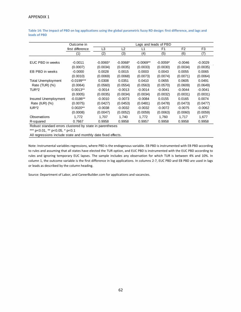
APPENDIX 1 

62  

Table 14: The impact of PBD on log applications using the global parametric fuzzy RD design: first difference, and lags and leads of PBD 

 

Note: Instrumental variables regressions, where PBD is the endogenous variable. EB PBD is instrumented with EB PBD according 

to rules and assuming that all states have elected the TUR option, and EUC PBD is instrumented with the EUC PBD according to 

rules  and  ignoring  temporary  EUC  lapses.  The  sample  includes  any  observation  for which  TUR  is  between  4%  and  10%.  In 

column 1, the outcome variable is the first difference in log applications. In columns 2‐7, EUC PBD and EB PBD are used in lags 

or leads as described by the column heading. 

Source: Department of Labor, and CareerBuilder.com for applications and vacancies. 

   

Outcome infirst difference L3 L2 L1 F1 F2 F3

(1) (2) (3) (4) (5) (6) (7)

EUC PBD in weeks -0.0011 -0.0065* -0.0068* -0.0069** -0.0059* -0.0046 -0.0029(0.0007) (0.0034) (0.0035) (0.0033) (0.0030) (0.0034) (0.0035)

EB PBD in weeks -0.0000 0.0028 0.0015 0.0003 0.0043 0.0055 0.0065(0.0010) (0.0069) (0.0068) (0.0073) (0.0074) (0.0071) (0.0064)

Total Unemployment -0.0199*** 0.0308 0.0351 0.0410 0.0655 0.0605 0.0491 Rate (TUR) (%) (0.0064) (0.0560) (0.0554) (0.0563) (0.0570) (0.0609) (0.0649)TUR 2̂ 0.0013** -0.0014 -0.0013 -0.0014 -0.0041 -0.0044 -0.0041

(0.0005) (0.0035) (0.0034) (0.0034) (0.0032) (0.0031) (0.0031)Insured Unemployment -0.0186** -0.0010 -0.0073 -0.0084 0.0155 0.0165 0.0074 Rate (IUR) (%) (0.0075) (0.0427) (0.0453) (0.0481) (0.0478) (0.0473) (0.0477)IUR 2̂ 0.0020** -0.0038 -0.0032 -0.0032 -0.0072 -0.0075 -0.0062

(0.0008) (0.0047) (0.0052) (0.0059) (0.0063) (0.0060) (0.0059)Observations 1,772 1,707 1,740 1,772 1,760 1,717 1,677R-squared 0.7667 0.9958 0.9958 0.9957 0.9958 0.9958 0.9958Robust standard errors clustered by state in parentheses*** p<0.01, ** p<0.05, * p<0.1All regressions include state and monthly date fixed effects.

Lags and leads of PBD

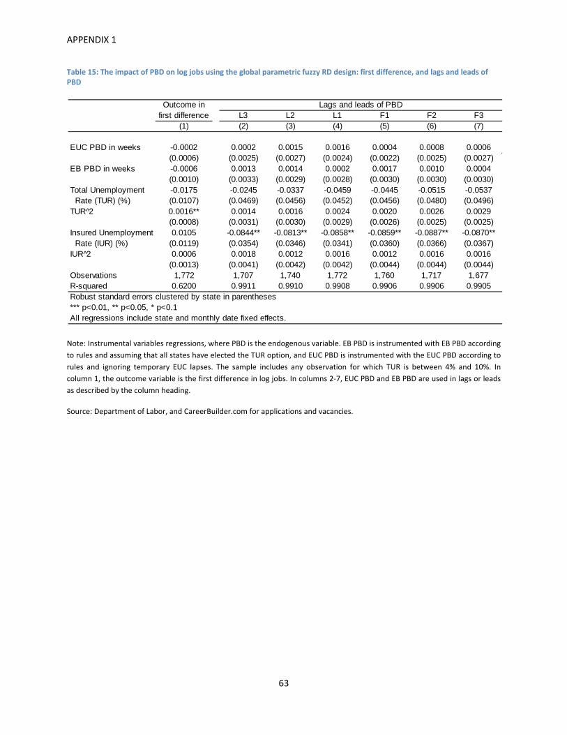
APPENDIX 1 

63  

Table 15: The impact of PBD on log jobs using the global parametric fuzzy RD design: first difference, and lags and leads of PBD 

 

Note: Instrumental variables regressions, where PBD is the endogenous variable. EB PBD is instrumented with EB PBD according 

to rules and assuming that all states have elected the TUR option, and EUC PBD is instrumented with the EUC PBD according to 

rules  and  ignoring  temporary  EUC  lapses.  The  sample  includes  any  observation  for which  TUR  is  between  4%  and  10%.  In 

column 1, the outcome variable is the first difference in log jobs. In columns 2‐7, EUC PBD and EB PBD are used in lags or leads 

as described by the column heading. 

Source: Department of Labor, and CareerBuilder.com for applications and vacancies.

Outcome infirst difference L3 L2 L1 F1 F2 F3

(1) (2) (3) (4) (5) (6) (7)

EUC PBD in weeks -0.0002 0.0002 0.0015 0.0016 0.0004 0.0008 0.0006(0.0006) (0.0025) (0.0027) (0.0024) (0.0022) (0.0025) (0.0027)

EB PBD in weeks -0.0006 0.0013 0.0014 0.0002 0.0017 0.0010 0.0004(0.0010) (0.0033) (0.0029) (0.0028) (0.0030) (0.0030) (0.0030)

Total Unemployment -0.0175 -0.0245 -0.0337 -0.0459 -0.0445 -0.0515 -0.0537 Rate (TUR) (%) (0.0107) (0.0469) (0.0456) (0.0452) (0.0456) (0.0480) (0.0496)TUR 2̂ 0.0016** 0.0014 0.0016 0.0024 0.0020 0.0026 0.0029

(0.0008) (0.0031) (0.0030) (0.0029) (0.0026) (0.0025) (0.0025)Insured Unemployment 0.0105 -0.0844** -0.0813** -0.0858** -0.0859** -0.0887** -0.0870** Rate (IUR) (%) (0.0119) (0.0354) (0.0346) (0.0341) (0.0360) (0.0366) (0.0367)IUR 2̂ 0.0006 0.0018 0.0012 0.0016 0.0012 0.0016 0.0016

(0.0013) (0.0041) (0.0042) (0.0042) (0.0044) (0.0044) (0.0044)Observations 1,772 1,707 1,740 1,772 1,760 1,717 1,677R-squared 0.6200 0.9911 0.9910 0.9908 0.9906 0.9906 0.9905Robust standard errors clustered by state in parentheses*** p<0.01, ** p<0.05, * p<0.1All regressions include state and monthly date fixed effects.

Lags and leads of PBD

APPENDIX 2 

64  

APPENDIX2:localparametricfuzzyregressiondiscontinuitydesignCrossing  a  threshold  in  the  total unemployment  rate  (TUR)  is much more  likely  to  lead  to  an  actual 

increase in PBD than crossing a threshold in the insured unemployment rate (IUR) (see p. 8). I therefore 

focus on TUR thresholds. Among all the TUR thresholds, the one at 6% TUR for EUC is the best candidate 

for a regression discontinuity design because  it applies to all states. Moreover, around 6% TUR, states 

would typically not have extended benefits (EB).  Indeed, TUR must be above 6.5%  in the states with a 

TUR option for EB to be turned on.  By contrast, the next EUC TUR threshold is met at 8.5%, which would 

trigger EB in states that have an 8% TUR threshold for EB. The potential triggering of EB would introduce 

additional interpretation issues, thus the EUC discontinuity around 6% is a better option. 

Increases  in PBD occur at specific TUR thresholds  (Figure 14). The data  in the  figure  is at the week by 

state level for December 2008 to October 2009, a period during which the PBD schedule as a function of 

TUR was constant. Two main reasons justify the limitation of observations to December 2008 to October 

2009. First, prior to December 2008, EUC did not depend on TUR, and after October 2009, PBD increased 

at more TUR  thresholds. Second, after October 2009,  there were  few states with TUR  just below 6%, 

making that latter period unsuitable for a regression discontinuity design around 6% TUR.  

If we focus on 1 percentage point around 6% TUR (i.e. 5.5% TUR to 6.4% TUR) then no clear discontinuity 

in PBD is observed (Appendix 2, Figure 14, blue hollow circles). This is because some states are eligible 

for EB or EUC under  IUR conditions, which means that PBD can be at a higher  level even when TUR  is 

below 6%. Additionally, even when TUR  is above 6%,  some  states have  the  lower PBD  level because 

there  is  usually  a  delay  between  when  a  state  crosses  the  threshold  and  when  benefits  become 

available.  To  focus  on  a  situation where  PBD  only  depends  on  TUR  (and  not  IUR),  and  to  apply  a 

standard  fuzzy  regression  discontinuity  design,  I  exclude  some  of  the  observations.  First,  state‐week 

observations are dropped where any EB  is available due  to  IUR conditions. Second,  I also drop  state‐

week observations where TUR  is below 6%  and  the  IUR  condition  for EUC  is  satisfied.  Substantively, 

what these exclusions do  is drop the 15% of state‐week observations42  in the 5.5% to 6.4% TUR range 

where  IUR  is unusually high compared  to TUR. This procedure  leaves only observations where TUR  is 

between 5.5% to 6.4% and PBD is either 46 or 59 weeks (red diamonds in Appendix 2, Figure 14).  

                                                            42  If we don’t exclude these observations, the point estimates for the  impact of PBD  in Appendix 2, Table 16 are essentially unchanged. 

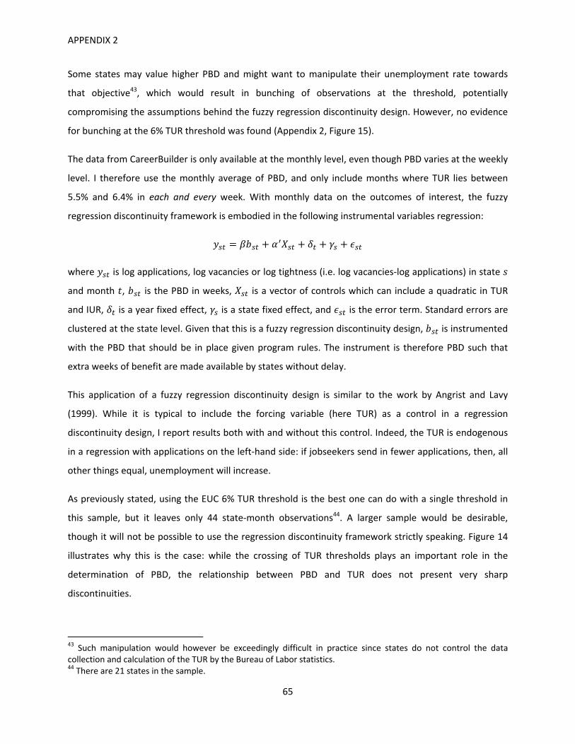
APPENDIX 2 

65  

Some  states may value higher PBD and might want  to manipulate  their unemployment  rate  towards 

that  objective43,  which  would  result  in  bunching  of  observations  at  the  threshold,  potentially 

compromising the assumptions behind the fuzzy regression discontinuity design. However, no evidence 

for bunching at the 6% TUR threshold was found (Appendix 2, Figure 15).  

The data from CareerBuilder is only available at the monthly level, even though PBD varies at the weekly 

level.  I  therefore use  the monthly average of PBD, and only  include months where TUR  lies between 

5.5%  and  6.4%  in  each  and  every week. With monthly  data  on  the  outcomes  of  interest,  the  fuzzy 

regression discontinuity framework is embodied in the following instrumental variables regression: 

 

where   is log applications, log vacancies or log tightness (i.e. log vacancies‐log applications) in state   

and month  ,    is the PBD  in weeks,    is a vector of controls which can  include a quadratic  in TUR 

and IUR,   is a year fixed effect,   is a state fixed effect, and   is the error term. Standard errors are 

clustered at the state level. Given that this is a fuzzy regression discontinuity design,   is instrumented 

with  the PBD  that should be  in place given program  rules. The  instrument  is  therefore PBD such  that 

extra weeks of benefit are made available by states without delay.  

This  application of  a  fuzzy  regression discontinuity design  is  similar  to  the work by Angrist  and  Lavy 

(1999).  While  it  is  typical  to  include  the  forcing  variable  (here  TUR)  as  a  control  in  a  regression 

discontinuity design, I report results both with and without this control. Indeed, the TUR is endogenous 

in a regression with applications on the left‐hand side: if jobseekers send in fewer applications, then, all 

other things equal, unemployment will increase. 

As previously stated, using the EUC 6% TUR threshold  is the best one can do with a single threshold  in 

this  sample,  but  it  leaves  only  44  state‐month  observations44.  A  larger  sample would  be  desirable, 

though it will not be possible to use the regression discontinuity framework strictly speaking. Figure 14 

illustrates why  this  is  the  case: while  the  crossing  of  TUR  thresholds  plays  an  important  role  in  the 

determination  of  PBD,  the  relationship  between  PBD  and  TUR  does  not  present  very  sharp 

discontinuities.  

                                                            43  Such manipulation would  however  be  exceedingly  difficult  in  practice  since  states  do  not  control  the  data collection and calculation of the TUR by the Bureau of Labor statistics. 44 There are 21 states in the sample. 

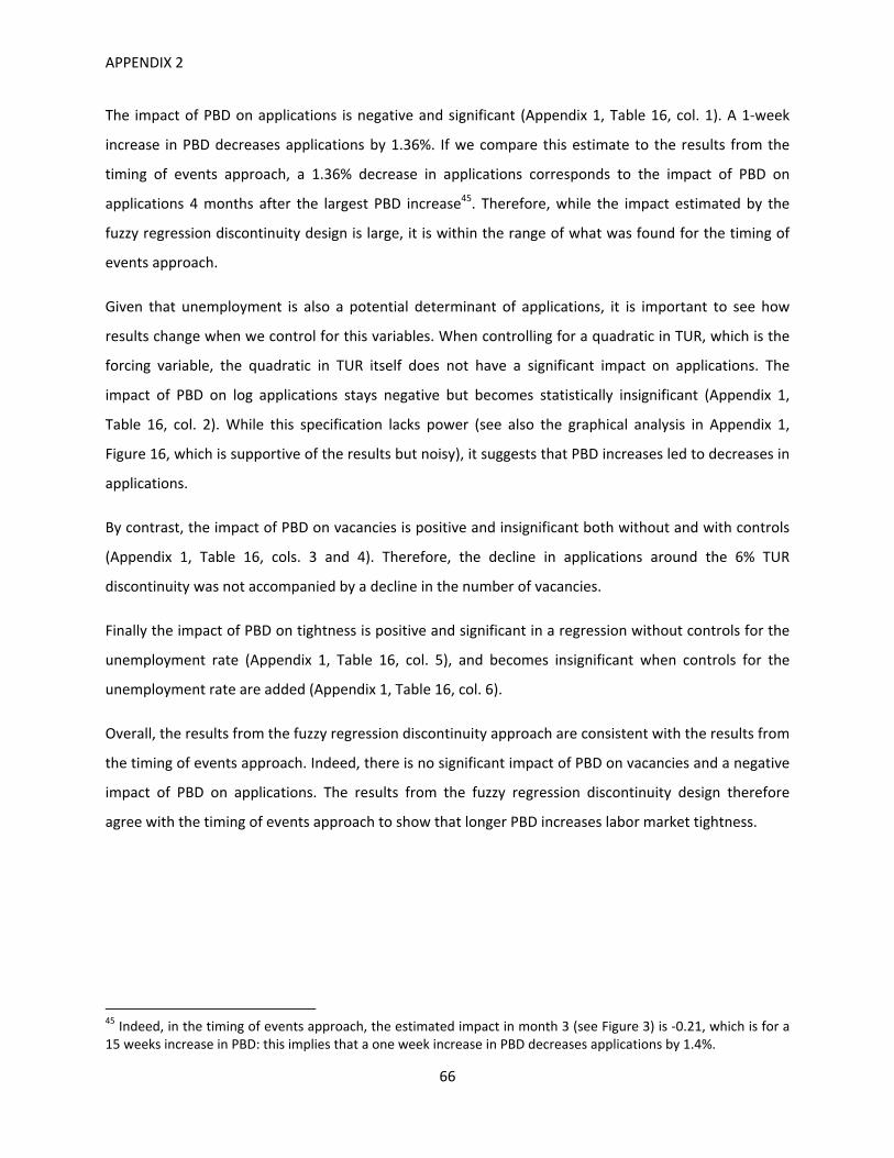
APPENDIX 2 

66  

The  impact of PBD on applications  is negative and significant  (Appendix 1, Table 16, col. 1). A 1‐week 

increase  in PBD decreases applications by 1.36%.  If we compare  this estimate  to  the  results  from  the 

timing  of  events  approach,  a  1.36%  decrease  in  applications  corresponds  to  the  impact  of  PBD  on 

applications 4 months after  the  largest PBD  increase45. Therefore, while  the  impact estimated by  the 

fuzzy regression discontinuity design is large, it is within the range of what was found for the timing of 

events approach. 

Given  that unemployment  is also a potential determinant of applications,  it  is  important  to  see how 

results change when we control for this variables. When controlling for a quadratic in TUR, which is the 

forcing  variable,  the  quadratic  in  TUR  itself  does  not  have  a  significant  impact  on  applications.  The 

impact  of  PBD  on  log  applications  stays  negative  but  becomes  statistically  insignificant  (Appendix  1, 

Table  16,  col.  2). While  this  specification  lacks power  (see  also  the  graphical  analysis  in Appendix  1, 

Figure 16, which is supportive of the results but noisy), it suggests that PBD increases led to decreases in 

applications.  

By contrast, the impact of PBD on vacancies is positive and insignificant both without and with controls 

(Appendix  1,  Table  16,  cols.  3  and  4).  Therefore,  the  decline  in  applications  around  the  6%  TUR 

discontinuity was not accompanied by a decline in the number of vacancies. 

Finally the impact of PBD on tightness is positive and significant in a regression without controls for the 

unemployment  rate  (Appendix  1,  Table  16,  col.  5),  and  becomes  insignificant when  controls  for  the 

unemployment rate are added (Appendix 1, Table 16, col. 6). 

Overall, the results from the fuzzy regression discontinuity approach are consistent with the results from 

the timing of events approach. Indeed, there is no significant impact of PBD on vacancies and a negative 

impact  of  PBD  on  applications.  The  results  from  the  fuzzy  regression  discontinuity  design  therefore 

agree with the timing of events approach to show that longer PBD increases labor market tightness.  

                                                            45 Indeed, in the timing of events approach, the estimated impact in month 3 (see Figure 3) is ‐0.21, which is for a 15 weeks increase in PBD: this implies that a one week increase in PBD decreases applications by 1.4%. 

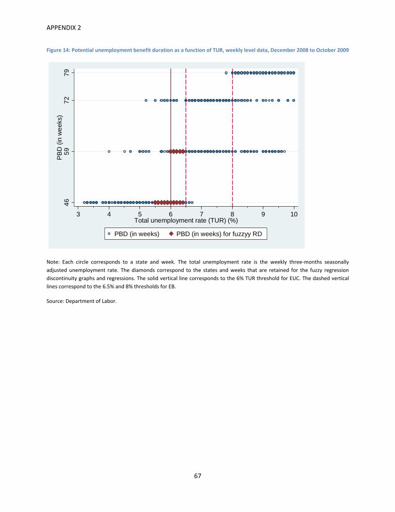
APPENDIX 2 

67  

Figure 14: Potential unemployment benefit duration as a function of TUR, weekly level data, December 2008 to October 2009 

 

Note:  Each  circle  corresponds  to  a  state  and week.  The  total  unemployment  rate  is  the weekly  three‐months  seasonally 

adjusted unemployment  rate. The diamonds  correspond  to  the  states and weeks  that are  retained  for  the  fuzzy  regression 

discontinuity graphs and regressions. The solid vertical line corresponds to the 6% TUR threshold for EUC. The dashed vertical 

lines correspond to the 6.5% and 8% thresholds for EB. 

Source: Department of Labor. 

46

59

72

79

PB

D (

in w

eek

s)

3 4 5 6 7 8 9 10Total unemployment rate (TUR) (%)

PBD (in weeks) PBD (in weeks) for fuzzyy RD

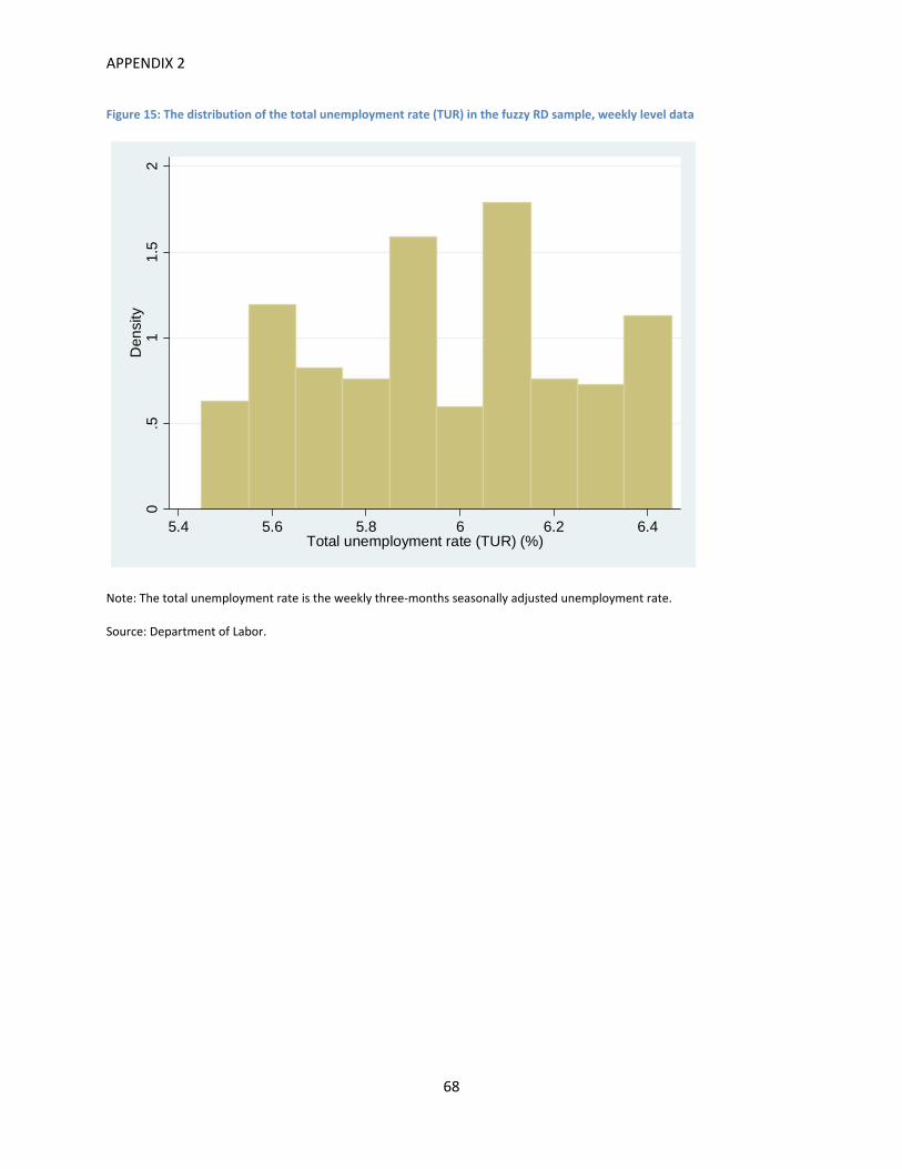
APPENDIX 2 

68  

Figure 15: The distribution of the total unemployment rate (TUR) in the fuzzy RD sample, weekly level data 

 

Note: The total unemployment rate is the weekly three‐months seasonally adjusted unemployment rate.  

Source: Department of Labor. 

0.5

11

.52

Den

sity

5.4 5.6 5.8 6 6.2 6.4Total unemployment rate (TUR) (%)

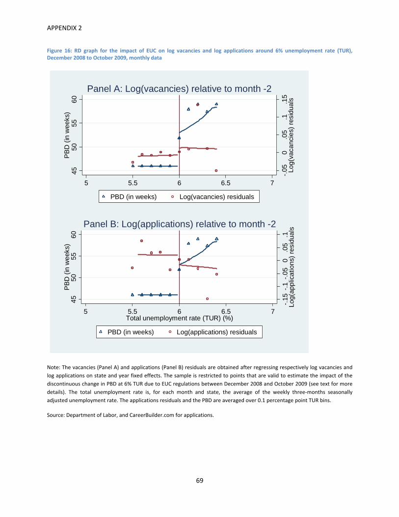
APPENDIX 2 

69  

Figure  16: RD  graph  for  the  impact  of  EUC  on  log  vacancies  and  log  applications  around  6%  unemployment  rate  (TUR), December 2008 to October 2009, monthly data 

 

Note: The vacancies (Panel A) and applications (Panel B) residuals are obtained after regressing respectively log vacancies and 

log applications on state and year fixed effects. The sample is restricted to points that are valid to estimate the impact of the 

discontinuous change in PBD at 6% TUR due to EUC regulations between December 2008 and October 2009 (see text for more 

details).  The  total  unemployment  rate  is,  for  each month  and  state,  the  average  of  the weekly  three‐months  seasonally 

adjusted unemployment rate. The applications residuals and the PBD are averaged over 0.1 percentage point TUR bins. 

Source: Department of Labor, and CareerBuilder.com for applications. 

-.05

0.0

5.1

.15

Log(

vaca

ncie

s) r

esid

uals

4550

5560

PB

D (

in w

eeks

)

5 5.5 6 6.5 7

PBD (in weeks) Log(vacancies) residuals

Panel A: Log(vacancies) relative to month -2

-.15

-.1

-.05

0.0

5.1

Log(

appl

icat

ions

) re

sidu

als

4550

5560

PB

D (

in w

eeks

)

5 5.5 6 6.5 7Total unemployment rate (TUR) (%)

PBD (in weeks) Log(applications) residuals

Panel B: Log(applications) relative to month -2

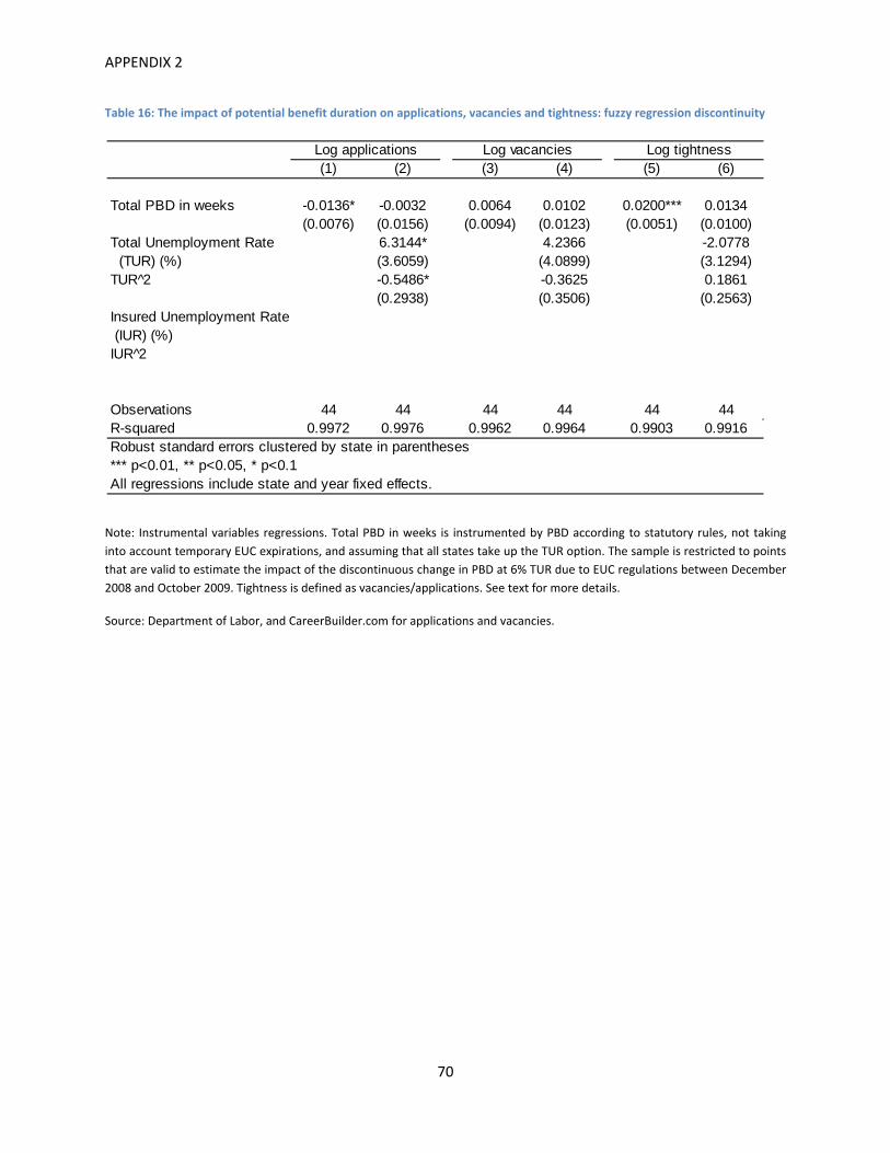
APPENDIX 2 

70  

Table 16: The impact of potential benefit duration on applications, vacancies and tightness: fuzzy regression discontinuity 

 

Note:  Instrumental variables regressions. Total PBD  in weeks  is  instrumented by PBD according  to statutory rules, not taking 

into account temporary EUC expirations, and assuming that all states take up the TUR option. The sample is restricted to points 

that are valid to estimate the impact of the discontinuous change in PBD at 6% TUR due to EUC regulations between December 

2008 and October 2009. Tightness is defined as vacancies/applications. See text for more details.  

Source: Department of Labor, and CareerBuilder.com for applications and vacancies. 

(1) (2) (3) (4) (5) (6)

Total PBD in weeks -0.0136* -0.0032 0.0064 0.0102 0.0200*** 0.0134(0.0076) (0.0156) (0.0094) (0.0123) (0.0051) (0.0100)

Total Unemployment Rate 6.3144* 4.2366 -2.0778 (TUR) (%) (3.6059) (4.0899) (3.1294)TUR^2 -0.5486* -0.3625 0.1861

(0.2938) (0.3506) (0.2563)Insured Unemployment Rate (IUR) (%)IUR^2

Observations 44 44 44 44 44 44R-squared 0.9972 0.9976 0.9962 0.9964 0.9903 0.9916Robust standard errors clustered by state in parentheses*** p<0.01, ** p<0.05, * p<0.1All regressions include state and year fixed effects.

Log applications Log vacancies Log tightness

APPENDIX 3 

71  

APPENDIX 3: additional specifications for the county pair differenceidentificationstrategyThis appendix presents additional  specifications  for  the  county pair difference  identification  strategy. 

Specifically, I  present regressions a la Hagedorn et al. (2013) and a la Dube, Lester, and Reich (2010).  

For the regressions a la Hagedorn et al. (2013), I adopt the following specification: 

Δ , Δ Δ  

where    is  the outcome    in county    in state   at date  .    is  the number of weeks of EUC 

available,   is the number of weeks of EB available. Δ ,  stands for a double difference: for county 

  in  state    and  its  paired  county  ′  in  state  ′, we  have Δ , , ,

′ ′ .   Δc stands for the difference across counties  in a pair at a given date  .    is a date fixed effect 

(monthly).   is the error term. 

The specification above was chosen to be as transparent as possible while still being very close to the 

one used by Hagedorn et al. (2013). There are two minor differences between this specification and the 

one used in Hagedorn et al. (2013). 

I take the undiscounted lead of the first difference46 of the outcomes over time. 

I  do  not  estimate  factor  loadings  for  common  time  effects  but  simply  use  a  set  of  time 

(monthly) dummies. Not using any time effects makes no difference to the qualitative results. 

For the regressions a la Dube, Lester, and Reich (2010), I use the following specification: 

 

where    is  the residual of outcome    in county    in state   at date  , after a regression of   on 

county  fixed  effects.  Similarly,    is  the  residual of  the number of weeks of  EUC  available  after 

county fixed effects, and   is the residual of the number of weeks of EB available after county fixed 

effects.   is a county pair by monthly date fixed effect.   is the error term, and standard errors are 

clustered by border segment, i.e. the set of all counties along a given state border. 

                                                            46  For  comparison,  I  have  also  run  as  specification  from  this  paper  that  relies  on  the  global  parametric  fuzzy regression discontinuity (i.e. in Table 3 and Table 4), but using the first difference of the outcome. PBD (EUC and EB)  has  no  significant  impact  on  the  first‐difference  of  applications  (Appendix  1  Table  14,  col.  1)  or  vacancies (Appendix 1, Table 15, col. 1), though EUC PBD still has a negative (insignificant) impact on applications. 

APPENDIX 3 

72  

The only difference between this specification and the one used in Dube, Lester, and Reich (2010) is the 

clustering  of  standard  errors:  for  simplicity,  I  use  border  segment  clustering,  rather  than  separately 

clustering on state and border segment. 

Both the regressions a  la Hagedorn et al. (2013) (Appendix 3, Table 17, col. 1‐3) and a  la Dube, Lester, 

and Reich (2010) (Appendix 3, Table 17, col. 4‐6) yield an insignificant effect of EUC PBD and EB PBD on 

applications, vacancies and labor market tightness. 

    

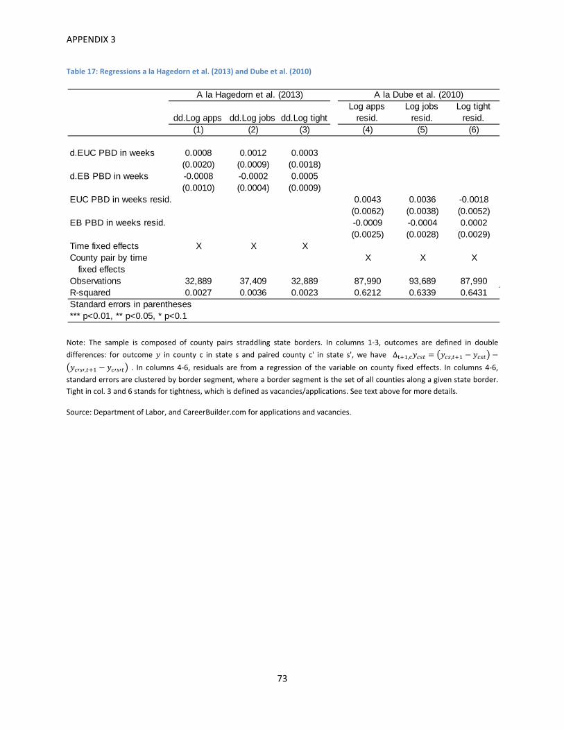
APPENDIX 3 

73  

Table 17: Regressions a la Hagedorn et al. (2013) and Dube et al. (2010) 

 

Note:  The  sample  is  composed  of  county  pairs  straddling  state  borders.  In  columns  1‐3,  outcomes  are  defined  in  double 

differences:  for outcome    in  county  c  in  state  s  and paired  county  c'  in  state  s', we have   Δ , ,

,   .  In  columns 4‐6,  residuals are  from a  regression of  the variable on  county  fixed effects.  In  columns 4‐6, 

standard errors are clustered by border segment, where a border segment is the set of all counties along a given state border. 

Tight in col. 3 and 6 stands for tightness, which is defined as vacancies/applications. See text above for more details. 

Source: Department of Labor, and CareerBuilder.com for applications and vacancies. 

 

dd.Log apps dd.Log jobs dd.Log tightLog apps

resid.Log jobs

resid.Log tight

resid.(1) (2) (3) (4) (5) (6)

d.EUC PBD in weeks 0.0008 0.0012 0.0003(0.0020) (0.0009) (0.0018)

d.EB PBD in weeks -0.0008 -0.0002 0.0005(0.0010) (0.0004) (0.0009)

EUC PBD in weeks resid. 0.0043 0.0036 -0.0018(0.0062) (0.0038) (0.0052)

EB PBD in weeks resid. -0.0009 -0.0004 0.0002(0.0025) (0.0028) (0.0029)

Time fixed effects X X XCounty pair by time X X X

fixed effectsObservations 32,889 37,409 32,889 87,990 93,689 87,990R-squared 0.0027 0.0036 0.0023 0.6212 0.6339 0.6431Standard errors in parentheses*** p<0.01, ** p<0.05, * p<0.1

A la Hagedorn et al. (2013) A la Dube et al. (2010)