The Geiger-Müller Counter

INSTRUMENTS

The Geiger-Müller counter

Figure 1. Control panel of the

Geiger-Muller counter.

Switching on the instrument

Before switching on the instrument, make sure that the High Voltage control is on minimum (200 V on the switch and 0 V on the voltage tuner). Switch on the instrument (Power switch) and wait 1-2 minutes until the instrument warms up.

Settings

Timer: 60 s (for background measurement: 300 s) High Voltage: 600 V (the High Voltage value is always determined as the sum of the values on the two knobs).

Measurement

Reset the counter before each measurement (Reset button) and start the measurement using the Start button. The counting will stop automatically after the counting time has passed. You may stop the measurement any time by pushing the Stop button.

1. Before switching on the instrument, make sure that the High Voltage control is on minimum (200 V on the switch and 0 V on the voltage tuner).

2. Switch on the instrument (Power switch) and wait 1-2 minutes until the instrument warms up.

3. Do not turn off the instrument until you finished all the measurements. Make sure that all switches are set to the proper value, especially take care of the voltage values.

4. Never exceed the indicated high voltage!

5. Do not touch the end-window of the GM-tube or the surface of the radioactive samples.

6. Before switching off the instrument, make sure that the high voltage control knob is set to minimum.

Switching off the instrument

After the measurement turn the High Voltage to the lowest value and then switch off the instrument. Make sure there is no sample left in the tower.

MEASUREMENTS

I. Measure the characteristic curve of a GM tube. Find the working potential

1. Place the standard uranium sample (U200) on the uppermost shelf of the lead shield using the plastic holder.

2. Increase the voltage to 400 V, 420 V, 440 V, 450 V then up to 800 V in steps of 50 V. Measure the intensity (counts per minute, cpm) value at every voltage for 60 sec. No counting is expected below the GM threshold.

3. Plot the cpm values against voltage using the appropriate Excel datasheet by using the computer.

4. The vertical axis must begin at the 0 value.

5. Determine the working voltage of the tube,as a voltage value 100 V higher than the start of the plateau. Set this working voltage for the later measurements.

II. Determine the average background

1. Set the working voltage determined previously.

2. Run the counter for five minutes (300 s) with no sample inside the lead tower.

3. Divide the counts by five to obtain the average background intensity in cpm (counts per minute). This value must be subtracted from the cpm values measured in the following measurements.

III. Statistic characterization of the radioactive decay

1. Place the sample (U200) on the lowest shelf of the tower.

2. Measure the cpm value of the uranium sample five times (each one minute long) using the working voltage.

3. Calculate the average value, and the standard deviation (sx).

4. Place the measured values and the average value on a straight line. Mark the standard deviation [average ± sx] and double standard deviation [average ± 2·sx] intervals. Examine, how many of the five measured values fall within each interval.

IV. Determine the counting efficiency factor (CEF) at three different distances from the detector

1. Place the standard uranium sample (U200) at three different heights (highest, middle and lowest shelf) and measure the actual cpm values 3 times for 1 minute at each position. Get the average of the cpm values at each position and subtract the background intensity.

2. Calculate the counting efficiency factors (CEF) for each position.

The 236 mg standard uranium-oxide sample (308U) contains 200 mg uranium. It is known that 1 mg uranium radiates 12.4 particles per second, thus the sample’s absolute activity per minute can be calculated: 1 1200 60 12,4 149000 minmg s s− −⋅ ⋅ = , meaning that the sample emits this amount of particles per minute (A). From that, under given circumstances, the tube detects only I impulses per minute. Calculating the counting efficiency factor for the given position:

1149 000 min

I ICEF

A −= =

3. CEF can be used to determine the absolute activity of an unknown sample.

V. Determine the absolute activity of an unknown sample

1. Place the unknown sample (U-X) in the tower, to medium height.

2. Measure the cpm value three times for one minute. Calculate the average and subtract the background.

3. Convert the cpm value to counts per second (cps), and divide it by the counting efficiency factor obtained for the middle position.

4. The value obtained is the absolute activity of the sample in Becquerel (Bq).

Do not forget to complete the appropiate part of the Radioactive half-life measurement! It should appears as a separate chapter in your notebook.

After the measurement turn the High Voltage to the lowest value and then switch off the instrument. Make sure there is no sample left in the tower.

Radioactive half-life

MEASUREMENTS

The two measurements are carried out with two or three weeks difference.

It is important to note: the date and time of measurement, the position of the sample in the lead tower, and the type and identifier of the sample.

These data are required for the analysis after the second measurement (Table 1.).

I. Measure the average bacground intensity, the intensity of the uranium standard and the unknown

sample

1. Set the working voltage of the GM-tube to 600 V.

2. If you have already measured the background today, use that value. Otherwise: close the door of the empty lead tower and measure the background for 5 minutes. Dividing the measured value by 5 gives the average backgound B1 (cpm, counts/minute), which is to be substracted from all the other measured intensity values.

3. Measure the intensity of the uranium standard (UT) three times for one minute, and substract the background intensity (B1) from the average intensity value. The result will be U1.

4. Measure the intensity of the unknown sample (marked with XT) three times for one minute, and substract the background intensity (B1) from the average intensity value. The result will be X1. Record the results (B1, U1, X1) and the date in your lab report according to Table 1.

II. Repeat the measurement after two or three weeks and determine the average background

Repeat the measurement after 2 or 3 weeks the same way as in Experiment I. Record the results (B2, U2, X2) and the date in your lab report.

III. Determine the half life of the unknown sample and identify the isotope

1. Calculate the elapsed days (t) between the two measurement.

2. Calculate T1/2 using the equation below.

3. Take the logarithm of both sides and express T1/2.

4. Identify the unknown radioactive substance using Table 1.

Mesuring radioactive half-life

Table 1.

Number and date of the

measurement

Position of the sample

Background intensity (B)

Intensity of the uranium sample (U)

Intensity of the unknown sample (I)

1:

2:

T1/2 The name of the unknown sample:

2/12T

t

1

2

2

1

U

U

X

X =

Table 2. The half-life

and field of

application of some

radioactive isotopes

that are important

form a medical or

biophysical aspect.

Isotope Half-life Radiation Field of application

238U 4.5·109

years

α nuclear energy production

14C 5.5·103

years

β- radiocarbon dating

3H 12.4 years β- chemical tracer

60Co 5.3 years γ radiotherapy, sterilization

Shilling-test (vitamin B12)

45Ca 152 days β- research (Ca metabolism)

35S 87.3 days β- research

89Sr 51 days β- radiotherapy, bone metastases diagnostics (Ca

analogue)

59Fe 47.1 days β- iron metabolism test (in the spleen)

86Rb 19.5 days β-, γ research

32P 14.3 days β- research: DNA, ATP tracing

131I 8 days γ thyroid scintigraphy

133Xe 5.2 days γ ventilation scintigraphy

198Au 2.7 days β- radio-chemotherapy (brachytherapy)

115Cd 2.3 days β- research

24Na 14.6 hours β-, γ research (water homeostasis)

42K 12.4 hours β- blood circulation test

99mTc 6 hours γ scintigraphic tracer

19F 110 mins β+ PET contrast

82Rb 78 seconds β+ myocardium PET

Gamma-absorption and spectrometry

INSTRUMENTS

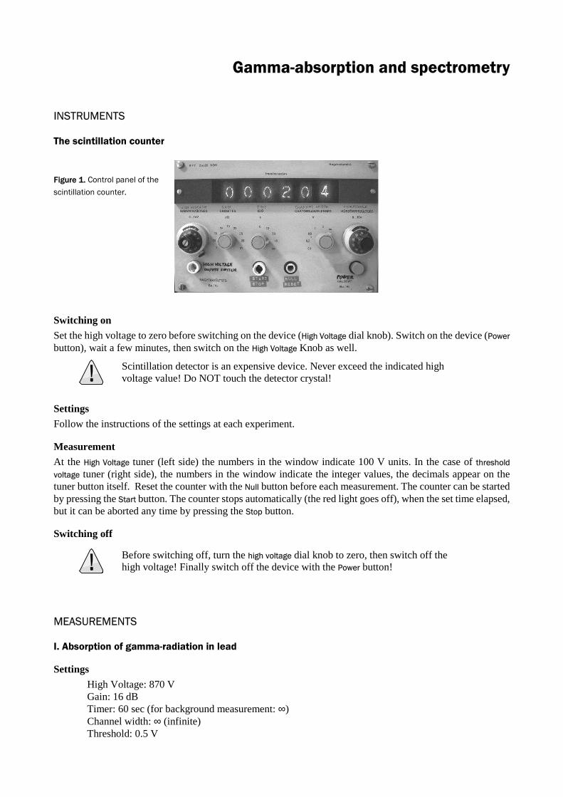
The scintillation counter

Figure 1. Control panel of the

scintillation counter.

Switching on

Set the high voltage to zero before switching on the device (High Voltage dial knob). Switch on the device (Power button), wait a few minutes, then switch on the High Voltage Knob as well.

Scintillation detector is an expensive device. Never exceed the indicated high voltage value! Do NOT touch the detector crystal!

Settings

Follow the instructions of the settings at each experiment.

Measurement

At the High Voltage tuner (left side) the numbers in the window indicate 100 V units. In the case of threshold

voltage tuner (right side), the numbers in the window indicate the integer values, the decimals appear on the tuner button itself. Reset the counter with the Null button before each measurement. The counter can be started by pressing the Start button. The counter stops automatically (the red light goes off), when the set time elapsed, but it can be aborted any time by pressing the Stop button.

Switching off

Before switching off, turn the high voltage dial knob to zero, then switch off the high voltage! Finally switch off the device with the Power button!

MEASUREMENTS

I. Absorption of gamma-radiation in lead

Settings

High Voltage: 870 V Gain: 16 dB Timer: 60 sec (for background measurement: ∞) Channel width: ∞ (infinite) Threshold: 0.5 V

1. Record the settings of the instrument in your lab report!

2. Measure the background without the sample. Set the timer to infinite and measure for five minutes, and divide the value by five to get the background intensity/minute. (Ibackground [cpm; counts per minute]). Use a stopwatch to measure the time elapsed and the Stop button to stop the counter.

3. Put the sample (137Cs) on the lowest shelf in the lead shield, to have enough room to place the absorber plates over the sample. Place the empty lead-holder frame over the sample.

4. Measure the count rate without absorber coins, but with an empty lead-holder frame 3 times for 1 minute. Place the absorber coins into the frame one by one and measure the count rates in each case 3 times for 1 minute (each coin is 2 mm thick). Calculate the average value for each absorber thickness and use the averages in the following.

5. Plot the count rates against the thickness of the absorber using the of the appropriate Excel file. Type the background intensity into the appropriate cell. The computer subtracts the background intensity from the average values and fits the curve. Read the half value layer from the graph and mark it, than calculate the linear absorption coefficient using the appropriate function.

II. Analyse the energy-spectrum of a gamma radiation

Settings

High Voltage: 870 V Gain: 16 dB Timer: 12 sec Channel width: 0.2 V Threshold: 8.0 V – 1.8 V (in steps of 0.2 V)

1. Record the settings of the instrument in your lab report!

2. Place the sample onto the highest shelf without the absorber-holder frame.

3. Use this energy selective counter to measure the count rate at a threshold of 8.0 V then reduce the threshold in steps of 0.2 V until 3 V, and measure the count rate at each setting. The channel width is 0.2 V, which determines the energy range of the measurable particles. As the threshold is reduced by 0.2 V steps you can scan the entire energy spectrum of the radioactive radiation of the sample.

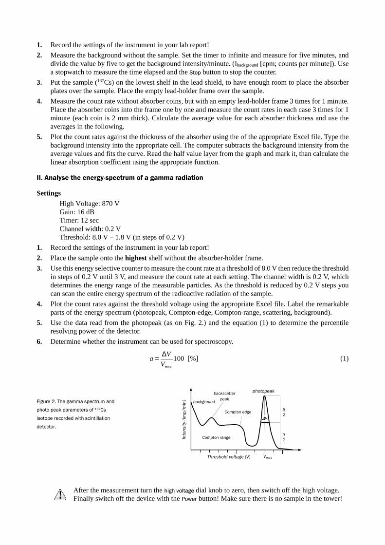
4. Plot the count rates against the threshold voltage using the appropriate Excel file. Label the remarkable parts of the energy spectrum (photopeak, Compton-edge, Compton-range, scattering, background).

5. Use the data read from the photopeak (as on Fig. 2.) and the equation (1) to determine the percentile resolving power of the detector.

6. Determine whether the instrument can be used for spectroscopy.

max

100∆= V

aV

[%] (1)

After the measurement turn the high voltage dial knob to zero, then switch off the high voltage. Finally switch off the device with the Power button! Make sure there is no sample in the tower!

Figure 2. The gamma spectrum and

photo peak parameters of 137Cs

isotope recorded with scintillation

detector.

Threshold voltage (V)

Inte

nsi

ty (

imp

/min

)

Vmax

2h

2h

background

backscatter

peak

Compton edge

photopeak

Compton range

∆V

Absorption of beta-radiation, dead-time

INSTRUMENTS

The Geiger-Müller counter

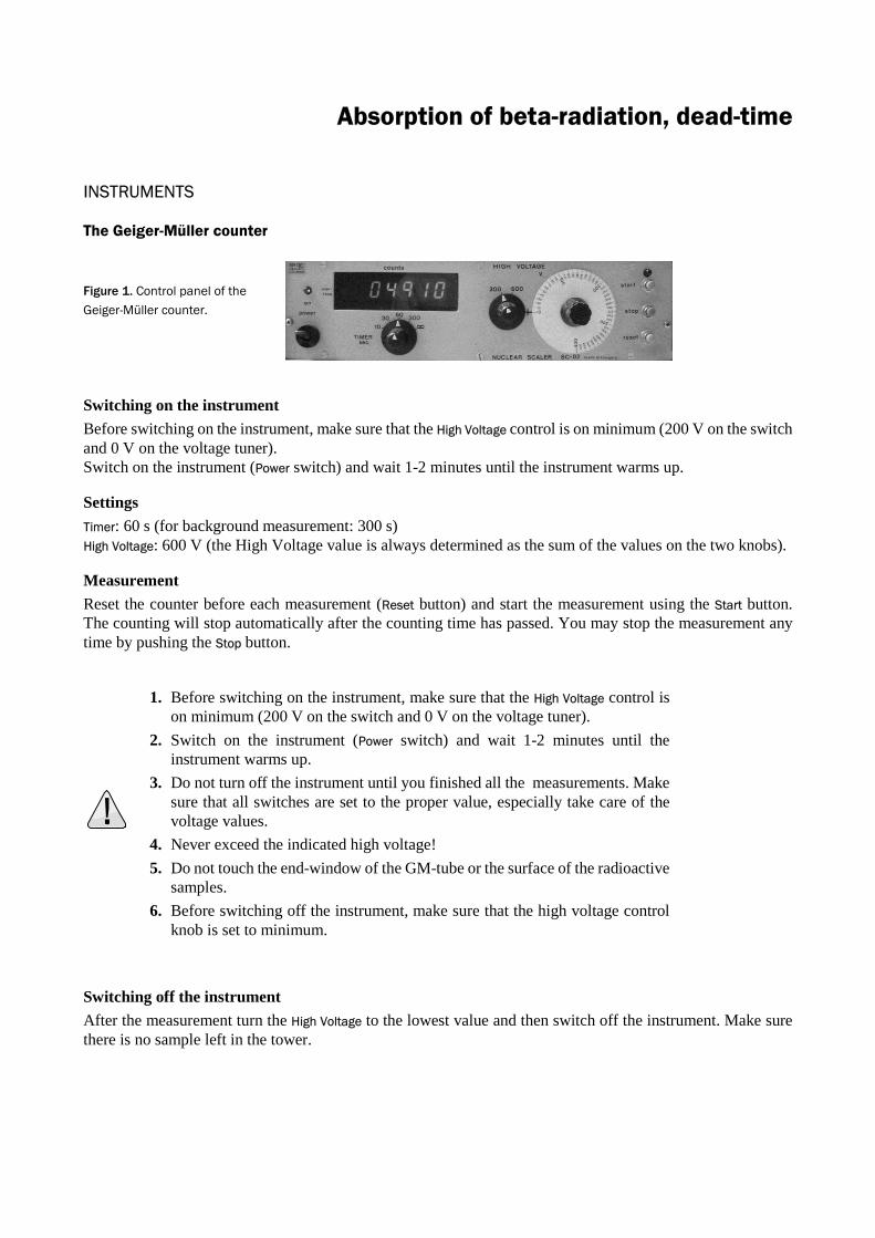
Figure 1. Control panel of the

Geiger-Müller counter.

Switching on the instrument

Before switching on the instrument, make sure that the High Voltage control is on minimum (200 V on the switch and 0 V on the voltage tuner). Switch on the instrument (Power switch) and wait 1-2 minutes until the instrument warms up.

Settings

Timer: 60 s (for background measurement: 300 s) High Voltage: 600 V (the High Voltage value is always determined as the sum of the values on the two knobs).

Measurement

Reset the counter before each measurement (Reset button) and start the measurement using the Start button. The counting will stop automatically after the counting time has passed. You may stop the measurement any time by pushing the Stop button.

1. Before switching on the instrument, make sure that the High Voltage control is on minimum (200 V on the switch and 0 V on the voltage tuner).

2. Switch on the instrument (Power switch) and wait 1-2 minutes until the instrument warms up.

3. Do not turn off the instrument until you finished all the measurements. Make sure that all switches are set to the proper value, especially take care of the voltage values.

4. Never exceed the indicated high voltage!

5. Do not touch the end-window of the GM-tube or the surface of the radioactive samples.

6. Before switching off the instrument, make sure that the high voltage control knob is set to minimum.

Switching off the instrument

After the measurement turn the High Voltage to the lowest value and then switch off the instrument. Make sure there is no sample left in the tower.

MEASUREMENTS

I. Determination of the background intensity

1. If you alredy mesured background intensity for the Radioactive half-life measurement, use that value and continue with Task II.

2. Set the working voltage to 600 V. Close the door of the empty tower and measure the background counts for 5 minutes.

3. Divide the counts by five to get the background intensity in cpm (counts per minute).

II. Determination of the absorption parameters of Beta-radiation in aluminium

1. Place the empty plastic absorber frame above the sample (Abs). Change only the absorber to thicker ones in the further measurements.

2. Measure the count rates first without absorber and then with different thickness absorbers, three times one minute each thickness. Calculate the average count value for each aluminium thickness (written on the frames).

3. Put the data and the background value into the computer. Plot the intensity values (after substracting the background) against the absorber thickness using the appropriate Excel file (Beta_absorption).

4. Use the printed graph to determine the thickness of the half value layer and calculate the absorption coefficient, and the maximal range of the beta particles.

III. Determining the dead-time of the GM-counter

1. To determine the dead time use the sample cut into two halves, marked as A and B. Use the screws to hold the samples. When only one of the halves is placed into the lead shield, use the fibreglass half to get the identical geometric arrangement.

2. Measure the cpm values for A and B separately, then together (IA, IB, IA+B,). Perform 3 measurements with each sample placed on the lowest and the highest shelf of the lead tower.

3. Calculate the impulse - difference in both cases using the formula: (IA+IB - IA+B)

4. Compare the IA + IB and IAB values in both cases. The difference between IA+B and IA+IB should be greater on the highest shelf (higher pulse density). When measured on the lowest shelf, the pulse density is lower, thus the dead time does not disturb the measurement. This fact shows that it is recommended to perform different GM-tube measurements with relatively low pulse density (< 10000 imp/min).

5. Calculate the dead time using the data recorded in the uppermost position and convert the result into milliseconds. Use the following formula:

−+= +

count

min

2 BA

BABA

II

IIIτ (1)

Do not forget to complete the appropiate part of the Radioactive half-life measurement! It should appears as a separate chapter in your notebook.

After the measurement turn the High Voltage to the lowest value and then switch off the instrument. Make sure there is no sample left in the tower.

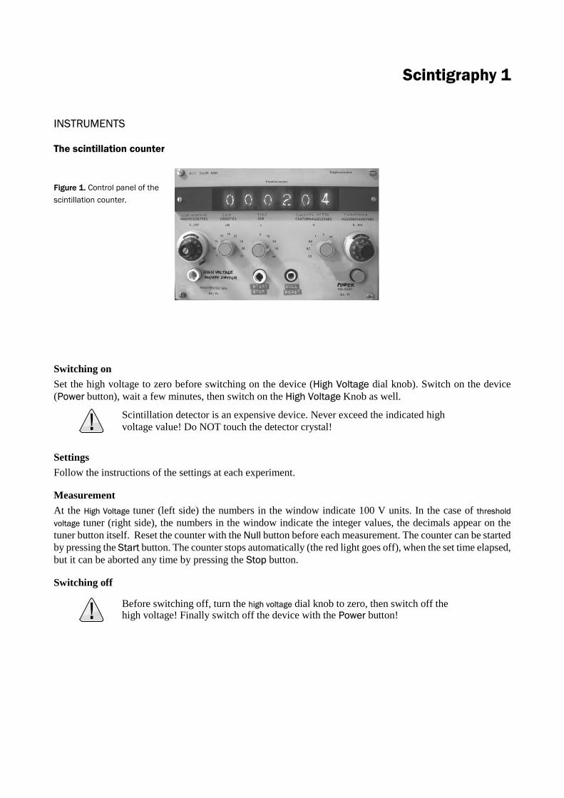
Scintigraphy 1

INSTRUMENTS

The scintillation counter

Figure 1. Control panel of the

scintillation counter.

Switching on

Set the high voltage to zero before switching on the device (High Voltage dial knob). Switch on the device (Power button), wait a few minutes, then switch on the High Voltage Knob as well.

Scintillation detector is an expensive device. Never exceed the indicated high voltage value! Do NOT touch the detector crystal!

Settings

Follow the instructions of the settings at each experiment.

Measurement

At the High Voltage tuner (left side) the numbers in the window indicate 100 V units. In the case of threshold

voltage tuner (right side), the numbers in the window indicate the integer values, the decimals appear on the tuner button itself. Reset the counter with the Null button before each measurement. The counter can be started by pressing the Start button. The counter stops automatically (the red light goes off), when the set time elapsed, but it can be aborted any time by pressing the Stop button.

Switching off

Before switching off, turn the high voltage dial knob to zero, then switch off the high voltage! Finally switch off the device with the Power button!

Scintigraphy 2

MEASUREMENTS

I. Determining the working potential of the scintillation detector

Settings

High Voltage: from 500 V to 900 V in steps of 50 V. Gain: 16 dB Time: 30 s Channel width: ∞ (infinite) Threshold: 0.1 V (Do not adjust!)

1. Adjust the parameters on the instrument written above. Measure the count rate without sample (A) over the voltage range indicated at the settings in steps of 50 V. This count rate corresponds to the noise (background, A).

2. Place the standard uranium sample exactly under the detector.

3. Measure the count rates at the same voltages as above. This gives the sum of the signal and the background (B). Pay attention not to move the detector and the sample during the measurement. Keep the sample in the glass container after finishing the measurement.

4. Type in the A and B values into the proper Excel table on the computer. The computer will automatically calculate the difference of the two impulse values that gives the signal (C=B-A), and calculates the signal-to-noise ratio (D), as well:

A

ABD

−= (1)

5. The program plots the parameters A, B, C and D against the voltage. The four curves should look similar to those shown in Figure 2.

Figure 2. Determination of the

working voltage

Note that the curves A, B and C have the same unit cpm, but the curve D is plotted as a set of relative values so a separate axis should be drawn on the figure (see left axis on Figure 2).

6. Find the optimal working voltage for the detector. This is indicated with an arrow on the figure, where the curves meet the following conditions: • low background (A) • high signal count rates (C) • moderate signal-to-noise ratio (D)

Sig

na

l / n

ois

e r

ati

o

Voltage

A

B

C

D Working voltage

A: background (noise) B: signal + noise

C: signal D: signal / noise

Imp

uls

e c

ou

nt

II. Explore the spatial distribution of the radioactive substance within the box

Settings

High Voltage: working potential determined in the first experiment. Gain: 16 dB Time: 12 s Channel width: ∞ (infinite) Threshold: 0.1 V (Do not adjust!)

1. Place the blue casette with the radioactive substances inside below the detector and measure the count rate starting at the position (A-1). Then repeat the measurement at each position of the box in the matrix from A-1 until I-7 (Figure 3). Collect the data in a table, similar as in Table 1.

Figure 3. Model of

scintigraphy.

Use the Excel file for data analysis.

Table 1.

Collecting

scintigraphy

data.

A B C D E F G H I

1

2

3

4

5

6

7

2. Enter the data into the Excel file on the computer, which will depict the distribution of the radioactive intensities in the form of a three-dimensional graph. Print out the graph and find the “hot” (high radiation) and the “cold” (low radiation) spots. Note down the coordinates of them.

3. Define which organ contains the “hot” spot!

The low activity places at the side of the trey are not „cold” spots. The real „cold” spots are surrounded completely by higher intensity areas.

A

12

B D G IC E F H

34

56

78

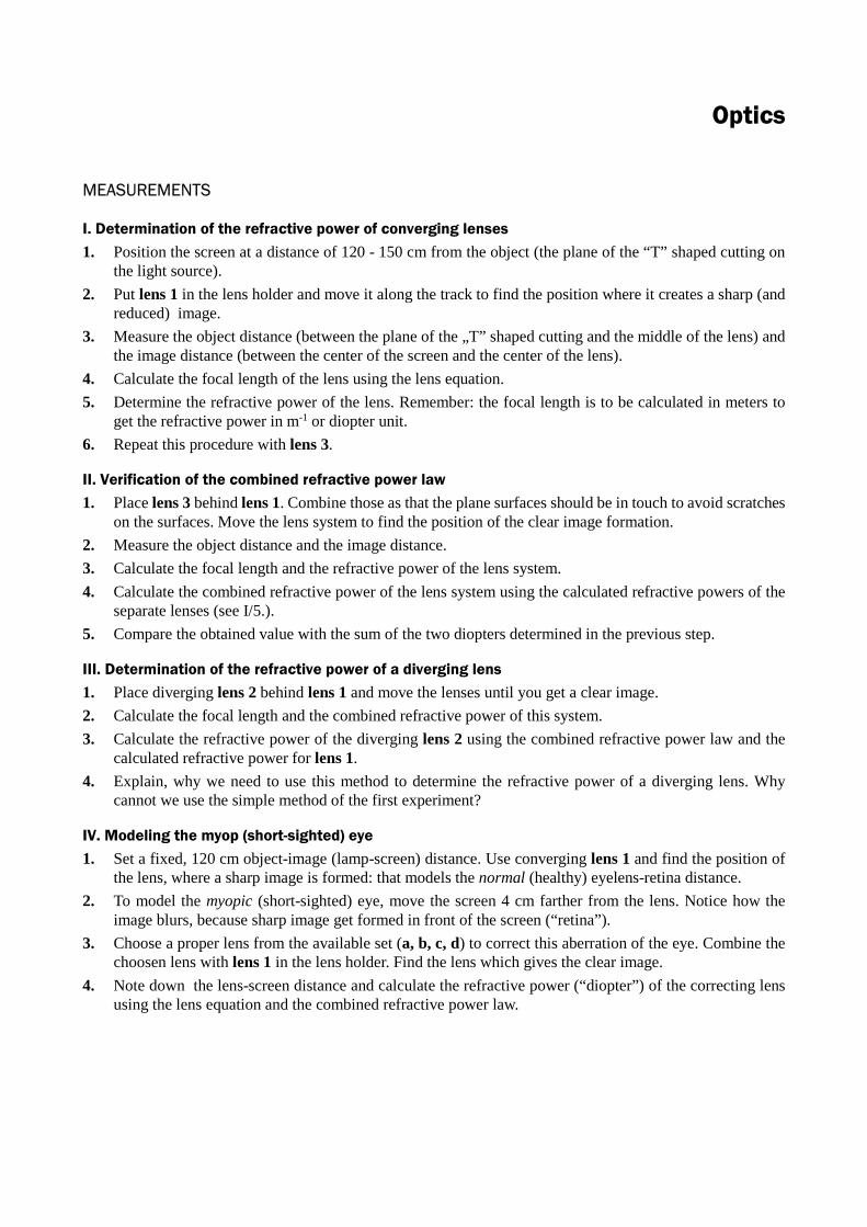
Optics

MEASUREMENTS

I. Determination of the refractive power of converging lenses

1. Position the screen at a distance of 120 - 150 cm from the object (the plane of the “T” shaped cutting on the light source).

2. Put lens 1 in the lens holder and move it along the track to find the position where it creates a sharp (and reduced) image.

3. Measure the object distance (between the plane of the „T” shaped cutting and the middle of the lens) and the image distance (between the center of the screen and the center of the lens).

4. Calculate the focal length of the lens using the lens equation.

5. Determine the refractive power of the lens. Remember: the focal length is to be calculated in meters to get the refractive power in m-1 or diopter unit.

6. Repeat this procedure with lens 3.

II. Verification of the combined refractive power law

1. Place lens 3 behind lens 1. Combine those as that the plane surfaces should be in touch to avoid scratches on the surfaces. Move the lens system to find the position of the clear image formation.

2. Measure the object distance and the image distance.

3. Calculate the focal length and the refractive power of the lens system.

4. Calculate the combined refractive power of the lens system using the calculated refractive powers of the separate lenses (see I/5.).

5. Compare the obtained value with the sum of the two diopters determined in the previous step.

III. Determination of the refractive power of a diverging lens

1. Place diverging lens 2 behind lens 1 and move the lenses until you get a clear image.

2. Calculate the focal length and the combined refractive power of this system.

3. Calculate the refractive power of the diverging lens 2 using the combined refractive power law and the calculated refractive power for lens 1.

4. Explain, why we need to use this method to determine the refractive power of a diverging lens. Why cannot we use the simple method of the first experiment?

IV. Modeling the myop (short-sighted) eye

1. Set a fixed, 120 cm object-image (lamp-screen) distance. Use converging lens 1 and find the position of the lens, where a sharp image is formed: that models the normal (healthy) eyelens-retina distance.

2. To model the myopic (short-sighted) eye, move the screen 4 cm farther from the lens. Notice how the image blurs, because sharp image get formed in front of the screen (“retina”).

3. Choose a proper lens from the available set (a, b, c, d) to correct this aberration of the eye. Combine the choosen lens with lens 1 in the lens holder. Find the lens which gives the clear image.

4. Note down the lens-screen distance and calculate the refractive power (“diopter”) of the correcting lens using the lens equation and the combined refractive power law.

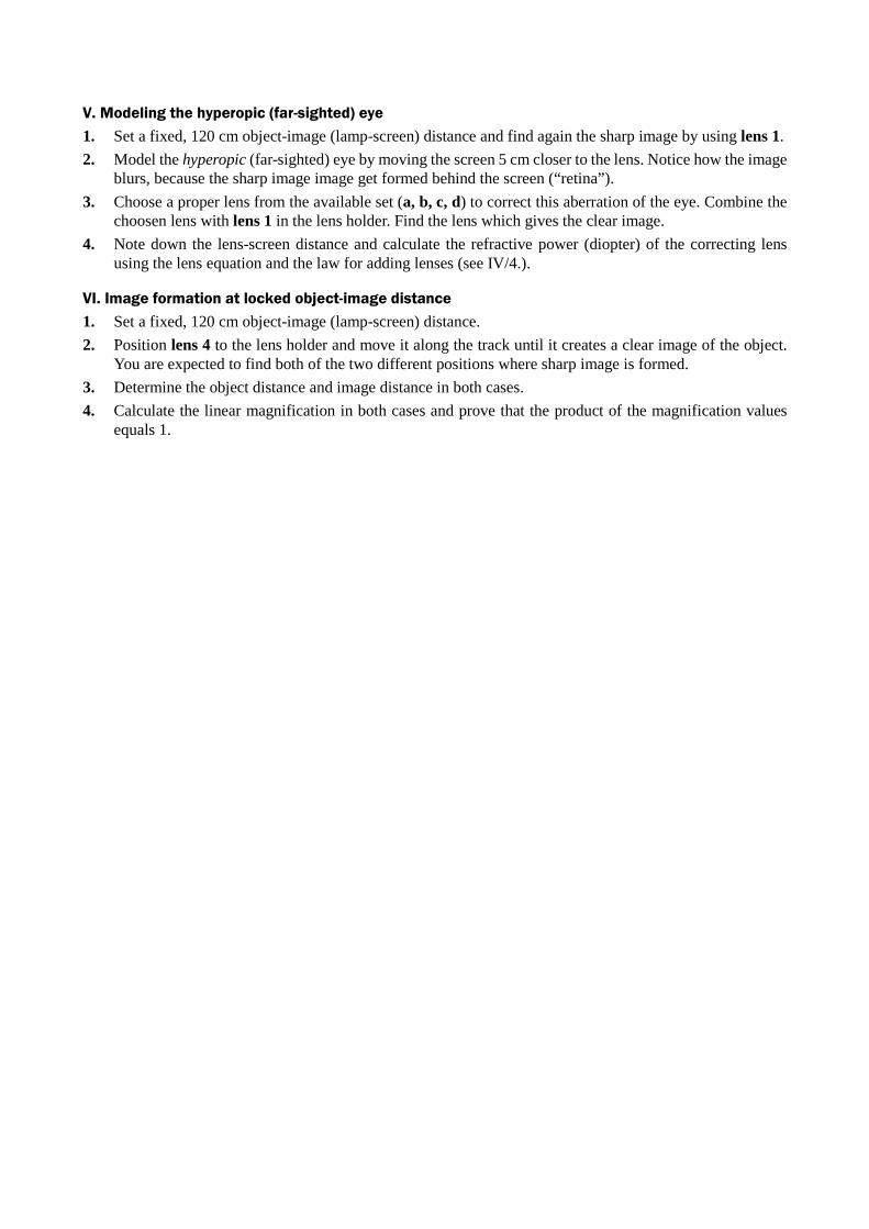
V. Modeling the hyperopic (far-sighted) eye

1. Set a fixed, 120 cm object-image (lamp-screen) distance and find again the sharp image by using lens 1.

2. Model the hyperopic (far-sighted) eye by moving the screen 5 cm closer to the lens. Notice how the image blurs, because the sharp image image get formed behind the screen (“retina”).

3. Choose a proper lens from the available set (a, b, c, d) to correct this aberration of the eye. Combine the choosen lens with lens 1 in the lens holder. Find the lens which gives the clear image.

4. Note down the lens-screen distance and calculate the refractive power (diopter) of the correcting lens using the lens equation and the law for adding lenses (see IV/4.).

VI. Image formation at locked object-image distance

1. Set a fixed, 120 cm object-image (lamp-screen) distance.

2. Position lens 4 to the lens holder and move it along the track until it creates a clear image of the object. You are expected to find both of the two different positions where sharp image is formed.

3. Determine the object distance and image distance in both cases.

4. Calculate the linear magnification in both cases and prove that the product of the magnification values equals 1.

Absorption photometry

INSTRUMENTS

Jasco V-550 UV/Vis Spectrophotometer and Spectra Manager software

Switching on

Switch on the photometer and wait 2 minutes. Switch on the PC and let the operation sytem boot, then start the Spectra Manager software. Select the Spectrum

Measurement program on the right window.

Setting the spectral parameters Measurement menu /Parameter submenu

Start: 550nm (maximum of the wavelength)

End: 350nm (minimum of the wavelength) Data Pitch: 1 nm

Scanning speed: 400 nm/min

After checking the settings press OK.

Measurements Repeat the following steps (Task I. – II. – III. ) for each pH level. Always perform 2 measurements: first measure the baseline with two cuvettes filled only with buffer (I.), then change one of the cuvettes for the fluorescein sample dissolved in the same buffer and measure its absorption spectrum (II. ).

Start the measurement with the lowest pH and continue in an increasing row! Between measurements rinse the cuvettes with distilled water! Hold the cuvettes by their graded sides, do not touch the transparent side of the cuvettes! When placing the cuvettes into the spectrophotometer, the light should go through the clear sides of each cuvette.

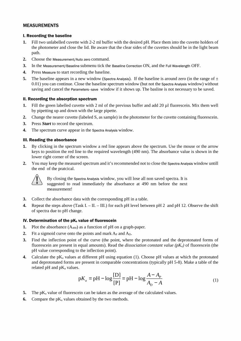
MEASUREMENTS

I. Recording the baseline

1. Fill two unlabelled cuvette with 2-2 ml buffer with the desired pH. Place them into the cuvette holders of the photometer and close the lid. Be aware that the clear sides of the cuvettes should be in the light beam path.

2. Choose the Measurement/Auto zero command.

3. In the Measurement/Baseline submenu tick the Baseline Correction ON, and the Full Wavelength OFF.

4. Press Measure to start recording the baseline.

5. The baseline appears in a new window (Spectra Analysis). If the baseline is around zero (in the range of ± 0.01) you can continue. Close the baseline spectrum window (but not the Spectra Analysis window) without saving and cancel the Parameters–save window if it shows up. The basline is not necessary to be saved.

II. Recording the absorption spectrum

1. Fill the green labelled cuvette with 2 ml of the previous buffer and add 20 µl fluorescein. Mix them well by pipetting up and down with the large pipette.

2. Change the nearer cuvette (labeled S, as sample) in the photometer for the cuvette containing fluorescein.

3. Press Start to record the spectrum.

4. The spectrum curve appear in the Spectra Analysis window.

III. Reading the absorbance

1. By clicking in the spectrum window a red line appears above the spectrum. Use the mouse or the arrow keys to position the red line to the required wavelength (490 nm). The absorbance value is shown in the lower right corner of the screen.

2. You may keep the measured spectrum and it’s recommended not to close the Spectra Analysis window untill the end of the pratcical.

By closing the Spectra Analysis window, you will lose all non saved spectra. It is suggested to read immediately the absorbance at 490 nm before the next measurement!

3. Collect the absorbance data with the corresponding pH in a table.

4. Repeat the steps above (Task I. – II. – III.) for each pH level between pH 2 and pH 12. Observe the shift of spectra due to pH change.

IV. Determination of the pKs value of fluorescein

1. Plot the absorbance (A490) as a function of pH on a graph-paper.

2. Fit a sigmoid curve onto the points and mark AP and AD.

3. Find the inflection point of the curve (the point, where the protonated and the deprotonated forms of fluorescein are present in equal amounts). Read the dissociation constant value (pKa) of fluorescein (the pH value corresponding to the inflection point).

4. Calculate the pKa values at different pH using equation (1). Choose pH values at which the protonated and deprotonated forms are present in comparable concentrations (typically pH 5-8). Make a table of the related pH and pKa values.

[D]

p pH log pH log[P]

Pa

D

A AK

A A

−= − = −− (1)

5. The pKa value of fluorescein can be taken as the average of the calculated values.

6. Compare the pKa values obtained by the two methods.

Blood pressure

INSTRUMENTS

Riva-Rocci’s sphygmomanometer

The indirect (non invasive) Riva-Rocci’s sphygmomanometer works as a mercury-column pressure gauge. The main components of the instrument are shown on Figure 1. The pressure I the cuff can be read from the scale beside the mercury column (manometer). The blood flow can be influenced by slight overpressure in the cuff and the most standard measuring technique employs either the palpation or audible detection of the pulse distal to an occlusive cuff .

Figure 1. Riva-Rocci’s

sphygmo-manometer.

Blood pressure is measured on the left upper arm for right-handers, generally.

The upper arm should be naked as any kind of clothes can disturb the measurement of blood pressure.

Position and tighten the cuff at the level of the heart on the upper arm to avoid the effect of hydrostatic pressure originating from height difference.

Blood pressure measurement with Riva-Rocci’s sphygmomanometer

1. Release the air from the occlusive cuff by opening the screw walve. Roll the empty cuff loosely around the upper arm in the middle region. Position the cuff as its lower side should be 1-2 cm far from the crook of the arm (Figure 2). Fix the cuff and close the valve of the pumping bulb.

Figure 2. The correct cuff

position.

2. Find the pulsating artery (arteria cubitalis) in the elbow-joint by palpation. The membrane or funnel of the phonendoscope is to be placed above this point later (Figure 3).

3. While sensing the radial pulse, inflate the occlusive cuff until the arteria brachialis closes up (when the radial pulse disappears). Increase the pressure in the cuff approximately 30 mmHg more.

Don’t hold the high pressure for long time as it blocks the blood and may result in grave impairment of the arm!

pumping bulb

screw valve

rubber tube

occlusive cuff manometer

Figure 3. The correct way

of ausculation and

palpation.

4. Place the membrane or funnel of the phonendoscope in the previously found position in the crook of the arm. You can’t hear anything by the phonendoscope because there is no blood flow.

5. Open the screwvalve gently to deflate the cuff pressure, about 2-3 mmHg per second. When the pressure in the cuff falls below the systolic pressure, the blood spurts under the cuff and causes a palpable pulse in the wrist. At the same time circulation starts through the narrowed vessel, we can hear the Korotkoff sound. The sound’s repetition rate is equal to the heart rate. When the cuff pressure is decreased by deflation under the diastolic pressure, the sound disappears (laminar flow).

6. On first detection of the pulse or sound read the manometer pressure which indicates the systolic pressure and read the diastolic pressure when the sound is about to disappear.

The automatic, electric sphygmomanometer

1. Switch on the sphygmomanometer and turn the cuff loosely around the upper arm (Figure 4). Wait until the automatic calibration finishes (a “0” appears on the display).

2. By pressing Start, the cuff inflates until about 150 mmHg, then the cuff pressure is automaticaly slowly deflated and the measurement starts.

3. At the end of the measurement the instrument automatically displays the results, systolic value is shown above the SYS sign, as diastolic is above the DIA sign, while after letter P the heart rate can be seen. Deflate the cuff after finishing the measurement.

Figure 4. Automatic

sphygmomanometer.

MEASUREMENTS

I. Measure of blood pressure with Riva-Rocci’s and automatic sphygmomanometer

Everyone should write down his/her own blood pressure values!

1. Measure your partner’s blood pressure at rest using Riva-Rocci’s and semi-automatic sphygmomanometer as well.

2. Right after some gymnastics (30 knee-bends), measure your partner’s blood pressure with both instruments. Start the measurements immediately after the gymnastics!

3. Exchange the roles with your partner and reppeat the measuerements.

4. Please write in your exercise book your own blood pressure results measured with both instruments, then convert the mmHg values to SI units, as kPa (1 mmHg = 0.1333 kPa). (You may read the kPa values directly from the scale of the mercury sphygmomanometer.)

Electrocardiography

MEASUREMENTS

I. Recording the ECG curve

Everyone should record and analyze his/her own ECG! The ECG curve should be sticked into the notebook!

1. Clear the electrodes where they get in contact with the skin, use alcoholic disinfecting solution!

2. To ensure proper contact, place a few ECG contact gel onto the electrodes.

3. Let your partner place the nippers on your limbs, on the right places (right arm – red, left arm – yellow, left leg – green, right leg – black, see Table 1.). During the ECG record comfortably lean back on your seat and place your legs on a chair. Do not move during the ECG is recorded, because any movement is accompanied by mechanical and electrical activity of muscles, which disturbs ECG recording. Do not touch the table or the chair with your hands. Be careful, your hands and legs should not get in touch (or should be covered by some dress).

Table 1. Standard limb leads (the

colour of electrodes in brackets).

Lead I right arm (red) – left arm (yellow)

Lead II right arm (red) – left leg (green)

Lead III left arm (yellow) – left leg (green)

Ground right leg (black)

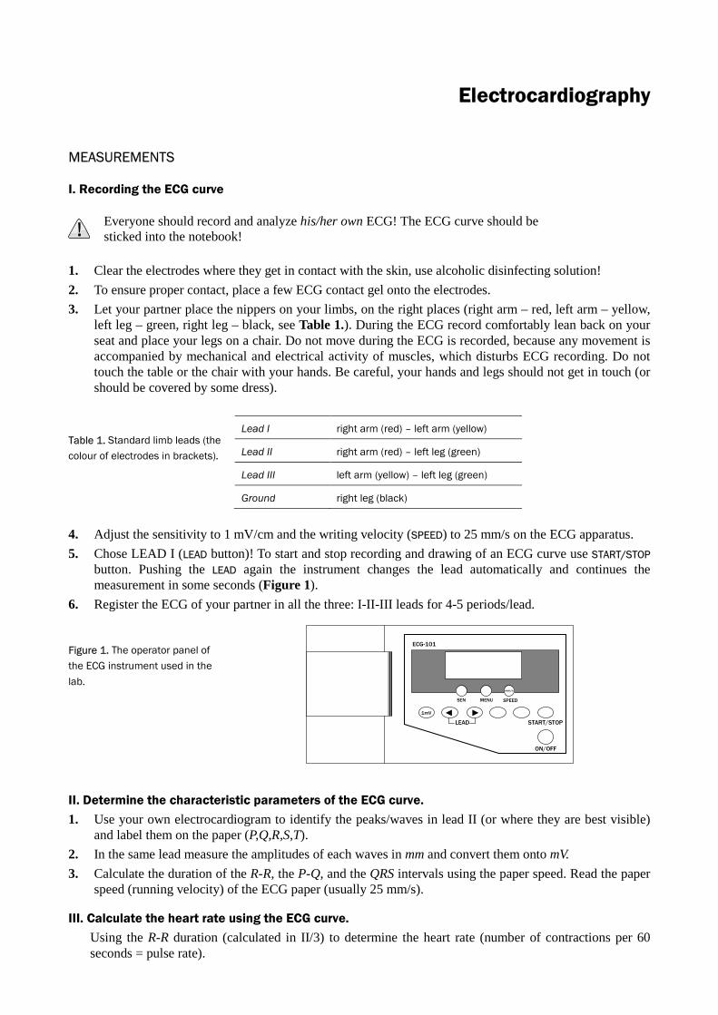
4. Adjust the sensitivity to 1 mV/cm and the writing velocity (SPEED) to 25 mm/s on the ECG apparatus.

5. Chose LEAD I (LEAD button)! To start and stop recording and drawing of an ECG curve use START/STOP button. Pushing the LEAD again the instrument changes the lead automatically and continues the measurement in some seconds (Figure 1).

6. Register the ECG of your partner in all the three: I-II-III leads for 4-5 periods/lead.

Figure 1. The operator panel of

the ECG instrument used in the

lab.

LEAD

ON/OFF

START/STOP

ECG-101

SPEED

1mV

mm/s

MENUSEN

II. Determine the characteristic parameters of the ECG curve.

1. Use your own electrocardiogram to identify the peaks/waves in lead II (or where they are best visible) and label them on the paper (P,Q,R,S,T).

2. In the same lead measure the amplitudes of each waves in mm and convert them onto mV.

3. Calculate the duration of the R-R, the P-Q, and the QRS intervals using the paper speed. Read the paper speed (running velocity) of the ECG paper (usually 25 mm/s).

III. Calculate the heart rate using the ECG curve.

Using the R-R duration (calculated in II/3) to determine the heart rate (number of contractions per 60 seconds = pulse rate).

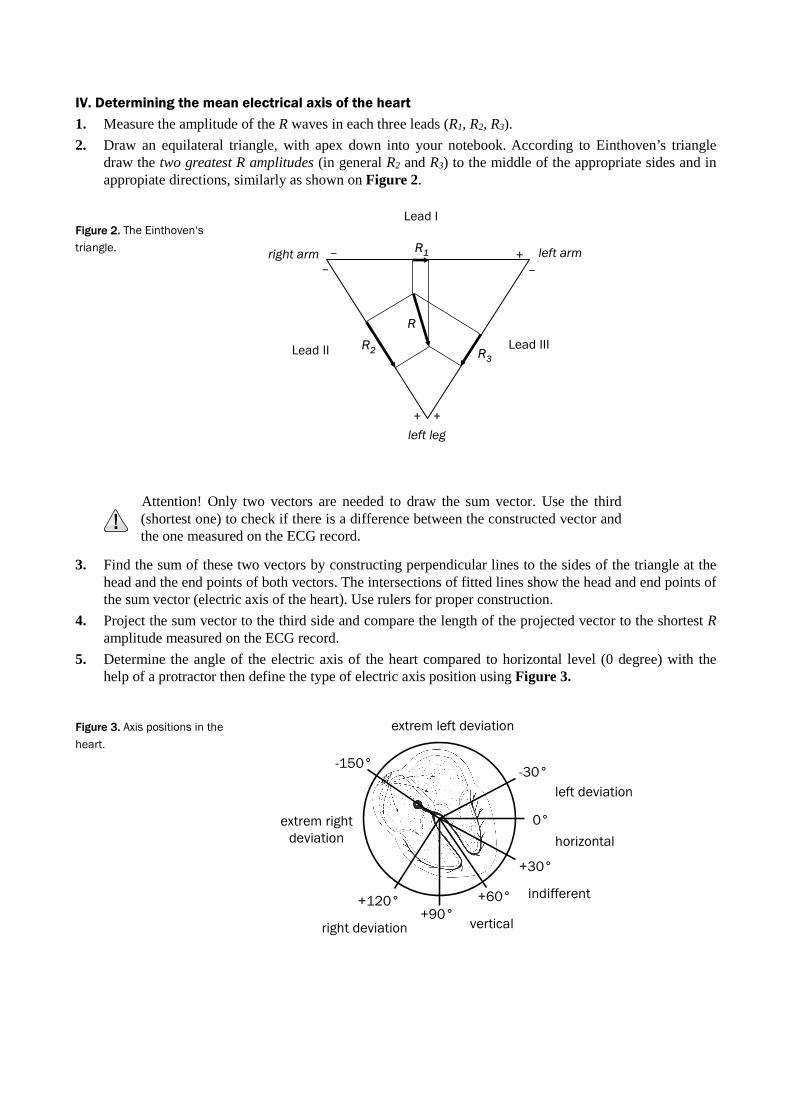
IV. Determining the mean electrical axis of the heart

1. Measure the amplitude of the R waves in each three leads (R1, R2, R3).

2. Draw an equilateral triangle, with apex down into your notebook. According to Einthoven’s triangle draw the two greatest R amplitudes (in general R2 and R3) to the middle of the appropriate sides and in appropiate directions, similarly as shown on Figure 2.

Figure 2. The Einthoven‘s

triangle.

–

Lead I

Lead II Lead III

R

R1

R2 R3

++

–

left leg

left armright arm–

+

Attention! Only two vectors are needed to draw the sum vector. Use the third (shortest one) to check if there is a difference between the constructed vector and the one measured on the ECG record.

3. Find the sum of these two vectors by constructing perpendicular lines to the sides of the triangle at the head and the end points of both vectors. The intersections of fitted lines show the head and end points of the sum vector (electric axis of the heart). Use rulers for proper construction.

4. Project the sum vector to the third side and compare the length of the projected vector to the shortest R amplitude measured on the ECG record.

5. Determine the angle of the electric axis of the heart compared to horizontal level (0 degree) with the help of a protractor then define the type of electric axis position using Figure 3.

Figure 3. Axis positions in the

heart.

-30°

0°

+30°

-150°

+60°

+90°+120°

indifferent

verticalright deviation

extrem right

deviation

extrem left deviation

left deviation

horizontal

Ultrasound

INSTRUMENTS

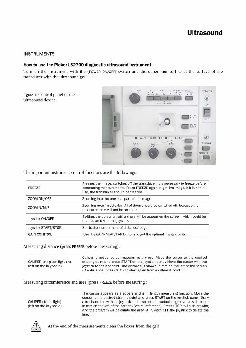
How to use the Picker LS2700 diagnostic ultrasound instrument

Turn on the instrument with the (POWER ON/OFF) switch and the upper monitor! Coat the surface of the transducer with the ultrasound gel!

Figure 1. Control panel of the ultrasound device.

The important instrument control functions are the followings:

FREEZE Freezes the image, switches off the transducer. It is necessary to freeze before conducting measurements. Press FREEZE again to get live image. If it is not in use, the transducer should be freezed.

ZOOM ON/OFF Zooming into the proximal part of the image

ZOOM N/M/F Zooming near/middle/far. All of them should be switched off, because the measurements will not be accurate

Joystick ON/OFF Swithes the cursor on/off, a cross will be appear on the screen, which could be manipulated with the joystick.

Joystick START/STOP Starts the measurment of distance/length

GAIN CONTROL Use the GAIN/NEAR/FAR buttons to get the optimal image quality.

Measuring distance (press FREEZE before measuring):

CALIPER on (green light on) (left on the keyboard)

Caliper is active, cursor appears as a cross. Move the cursor to the desired strating point and press START on the joystick panel. Move the cursor with the joystick to the endpoint. The distance is shown in mm on the left of the screen (D = distance). Press STOP to start again from a different point.

Measuring circumference and area (press FREEZE before measuring):

CALIPER off (no light) (left on the keyboard)

The cursor appears as a squere and is in length measuring function. Move the cursor to the desired strating point and press START on the joystick panel. Draw a freehand line with the joystick on the screen, the actual lengths value will appear in mm on the left of the screen (C=circumference). Press STOP to finish drawing and the program will calculate the area (A). Switch OFF the joystick to delete the line.

At the end of the measurements clean the boxes from the gel!

MEASUREMENTS

I. Checking the spatial calibration

1. Coat the linear transducer with ultrasound gel.

2. Place the transducer to the side of the water-filled plastic box .

3. Insert the glass rod into the container through one of the calibration holes on the lid. Identify the image of the glass rod on the screen.

4. Freeze the image and measure the on-screen distance of the glass rod from the transducer using the CALIPER on function. Record the on-screen distance for each calibration point.

5. Plot the on-screen distance against the real distance to obtain the spatial calibration curve on a graph paper. Fit a line over the points.

II. Propagation of ultrasound in glycerol and methanol

1. Measure the on-screen length of the water-filled plastic container, then the glycerol- and methanol-filled containers as well. (Find the most “bright” and linear line down on the screen for methanol.)

Warning: methanol is toxic! Do not open the container!

2. The instrument is calibrated for water, therefore it always uses the speed of sound in water (vwater=1500 m/s). Calculate the propagation speed of ultrasound in glycerol and methanol (vx) using equation (1):

waterx water

x

d

d=v v (1)

where dwater and dx are the on-screen distance of containers filled with water and the appropriate medium (glycerol or methanol, respectively).

3. Calculate the specific acoustic impedance of glycerol and methanol. The densities are: ρglycerol = 1260 kg/m3, ρmethanol = 791 kg/m3.

III. Calculating reflexivity on boundaries of media

Using the results of Task II , calculate the reflectivity (R) on the boundary of water-glycerol and methanol-water (the specific acoustic impedance of water: 1.49 x 106 rayle).

IV. Characterise the acoustic properties of various materials (water, air, Ca(OH)2 suspension)

1. Place the linear transducer to the side of the water-filled plastic container. Remove the cover and place the rubber fingers (one at a time) filled with various materials (water, air, Ca(OH)2 suspension) into the water-filled plastic container.

2. Draw a scheme and explain the images (on the basis of acoustic impedance and reflectivity).

V. Mapping the inner structure of a model box

1. Place the linear transducer to the side of the model box in a way that the reference point (X) should be on the side of the transducer, on its right side.

2. Move the transducer up and down to find the objects. According to the ultrasound image draw a 2D sketch image of the model box and measure the area and circumference of the objects in the box using the appropiate function of the instrument (CALIPER off)

VI. Bonus experiments

1. „Bonus box“

Examine the „Bonus box” in the same way as in the previous task. Find and identify the hidden objects.

2. Characterise the acoustic properties of the liver and the spleen

Place the transducer to the hepatic or splenic area of your standing laboratory partner, right under the right or left costal arc, respectively. Following deep inhalation the spleen and the liver are pushed by the diaphragm below the costal arc, and their examination becomes easier.

Temperature measurement

MEASUREMENTS

I. Determination of the calibration curves of the thermocouple and the thermistor

1. Connect the junctions of the thermocouple to the voltmeter.

2. Connect the termistor to the multimeter (COM and V/Ω junctions) and set the correct resistance (Ohm) range.

3. Put one end of the thermocouple into the ice-water mixture: this will be the cold point (0 °C).

4. Bring the water to boil and pour into the grey beaker to get approximately 80 °C water. Put the other end of the thermocouple into it: this will be the hot point.

5. Measure the temperature of the hot point using a thermometer. Record the temperature, the corresponding voltages of the thermocouple and the resistance of the thermistor.

Change the polarity of the connections if the pointer of the voltmeter moves in the negative direction.

6. Repeat this procedure by decreasing the temperature in 5-7 °C steps until approx. 20 °C. Add a small amounts of cold (tap) water to adjust the temperatures. Collect the date in a table!

II. Determination of the parameters of the thermocouple

1. Plot the voltage values of the thermocouple on a graph-paper as a function of temperature. Fit a linear curve onto the point through zero.

2. Determine the slope of the curve by reading the voltage difference corresponding to a certain temperature difference (e.g. 20 °C). Calculate the differential sensitivity of the thermocouple, which is the voltage difference in case of 1 °C temperature difference (in mV / °C unit).

III. Determination of the temperature of exhaled air, palm and neck

1. Take out the hot point of the thermocouple from the waterbath, dry it and hold it into the air. Wait until the voltage stabilizes. Record the value.

2. Repeat the measurement by holding the thermocouple to your palm and to your neck.

3. Convert the voltage values to temperature by using the calibration curve from Experiment II.

IV. Determination of different parameters of the thermistor

1. Evaluate the data of the thermistor using the corresponding Excel file on the computer.

Warning: the resistance should be given in ohm!

2. The computer program plot the resistance as a function of temperature and determines the parameters of the thermistor: the residual resistance and the activation energy.

3. Explain the result and define residual resistance (A) and the activation energy (∆E).

Audiometry

INSTRUMENTS

The sound generator and the audiometer

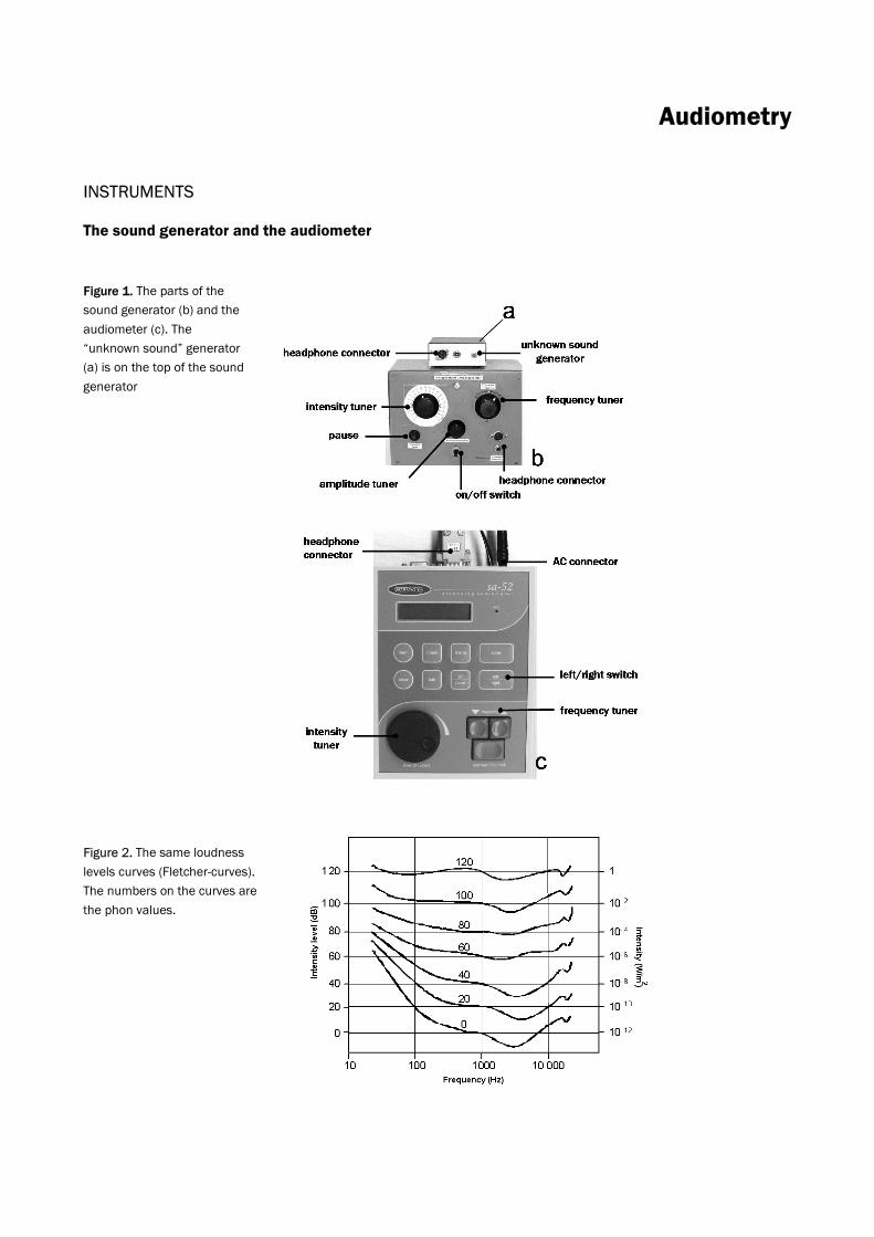
Figure 1. The parts of the

sound generator (b) and the

audiometer (c). The

“unknown sound” generator

(a) is on the top of the sound

generator

Figure 2. The same loudness

levels curves (Fletcher-curves).

The numbers on the curves are

the phon values.

MEASUREMENTS

Everyone should record and analyze his/her own hearing threshold and audiogram!

I. Record the threshold curve using a sound generator

1. Set the frequency control to 1000 Hz and the gain control to zero dB. Put the headphone on and use the amplitude button to adjust the volume until it is just hearable (find the threshold of hearing). The brake (pause) button may be used to decide whether you really heard the sound or not. Do not change the position of this amplitude control during further measurements!

2. Use the intensity knob to find your threshold of hearing at each frequency indicated on the frequency control knob.

3. Plot the threshold intensity against frequency with the computer.

4. Compare your curve with the standard Fletcher-curves (Figure 2).

II. Determination of two threshold-intensities on different frequencies

Calculate the absolute intensity (in W/m2 units) of two sounds from the Task I. giving acoustic sensation at the lowest and highest hearing threshold values. The reference intensity (the hearing threshold at 1000 Hz frequency) supposed to be 10-12 W/m2.

III. Recording audiogram 1. Take the headphone of the audiometer on, set it to fit properly and try to find its position when the noise

of the room is the lowest.

2. Set the frequency to 250 Hz (left button under the frequency sign) and set the intensity to -10 dB (level dB /

select turn knob). Choose the right or left ear (left/right button).

3. Increase the intensity by steps of 5 dB with the help of the intensity tuner.

4. When you hear the staccato sound, note the intensity value related to the given frequency.

5. To verify your result turn the intensity knob backwards (intensity decreases by 10 dB) and then start increasing the intensity in steps of 5 dB. Read the intensity value when you hear the pulsing sound again. If this sound is the same as you got previously you have found the intensity to the given frequency. If the two intensities are different, repeat the previous steps till you have the same results two times.

6. Increase the frequency and repeat the previous steps to measure the threshold intensities (at 500, 1000, 2000, 3000, 4000, 6000, 8000 Hz). Read and note the intensity values related to each frequency (Hz - dB) and collect them in a table (see below).

frequency (Hz)

intensity (dB)

left ear right ear

250

…

7. Repeat the steps after pressing the left/right button as well to get the data for both ears. (The Left sign changes to Right on the screen.) Start the measurement at 250 Hz at -10 dB.

You can not read the absolute intensity of the sound on the audiophon but you can read the loss of hearing which is the change from the normal hearing on a dB scale.

8. Plot the measured data on the paper handed out.

9. Compare the audiograms of your ears and note your observations (e.g. magnitude of the loss of hearing, is the loss of hearing the same at different frequencies or in the case of both ears).

IV. Determination of the loudness value of two sounds using the phon scale

1. Use the bifurcating wire to connect the headphones to the outputs of the sound generator (b) and the unknown tone generator (a) (Figure 1).

2. Switch on the 1st unknown sound (upper position).

3. Set the frequency on the sound generator to 1000 Hz (reference sound) and adjust the intensity (dB knob) until the loudness of the sounds in the two sides of the headphone are heard as equal. The loudness (phon) value equals with the dB value of the 1000 Hz sound if they are heard with the same loudness.

4. Record the intensity of the reference sound and determine the loudness (phon) value of the unknown sound.

5. Switch to the 2nd unknown sound (lower position) and repeat the measurement.

The results will be correct only if the audiograms of your ears are similar to the whole frequency range, that is, the audiograms recorded at Task III. of the ears are similar.