The Estimation of the Quenching Effects After Carburising ...cdn.intechopen.com/pdfs/32752/InTech-The... · The Estimation of the Quenching Effects After Carburising Using an Empirical

5

The Estimation of the Quenching Effects After Carburising Using an Empirical Way Based on Jominy Test Results

Mihai Ovidiu Cojocaru, Niculae Popescu and Leontin Drugă “POLITEHNICA” University, Bucharest,

Romania

1. Introduction

The graphical and analytical solutions to solve the information transfer from the Jominy test samples to real parts are shown. The essay regarding the analytical solutions for the information transfer from the Jominy test samples to real parts includes detailed information and exemplifications concerning the essence and using the Maynier-Carsi and Eckstein methods in order to determine the quenching constituents proportions corresponding to the different carbon concentrations in carburized layers, respectively the hardness profiles of the carburized and quenched layers. In the final of the chapter, taking into account the steel chemical composition, the geometrical characteristics of the carburized product, the quenching media characteristics, the heat and time parameters of the carburising and the correlations between these values and the Jominy test result, an algorithm to develop a software for the estimation of the quenching effects after carburising, based on the information provided by Jominy test, is proposed.

2. The particularities of quenching process after carburising

The aim of the quenching process after carburizing is to transform the “austenite” with high and variable carbon content of the carburized layer in quenching "martensite", respectively the core austenite in non martensitic constituents (bainite, quenching troostite, and ferrite-perlite mixture). This goal is achieved by transferring the parts from carburizing furnace into a cooling bath containing a liquid cooling (quenching) medium. The transfer can be directly made from the carburizing temperature (direct quenching), or after a previous pre-cooling of parts from the carburizing temperature to a lower quenching temperature (direct quenching with pre-cooling). In both ways, the austenitic grain size is the same (depending on the chosen carburising temperature and time), but the thermal stresses are different, being higher in the case of direct quenching and lower in the case of direct quenching with pre-cooling, due to higher thermal gradient achieved in the first cooling variant. Consequently, the risks of deformation or cracking of the parts are lower in the pre-cooling quenching, this variant being most commonly used in the industrial practice.

On the other hand, the result of quenching is influenced by three factors: one internal,

intrinsic hardenability of steel (determined by its chemical composition - carbon content,

www.intechopen.com

Recent Researches in Metallurgical Engineering – From Extraction to Forming

92

alloying elements type and percentage) and two external (technological) - thickness of the

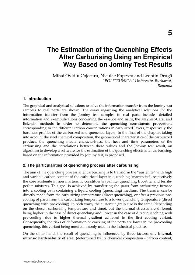
parts, expressed by an equivalent diameter Dech (the actual diameter in the case of cylindrical parts, or the diameter calculated using empirical relations for the parts with non cylindrical shapes) and cooling capacity of quenching media, expressed by relative cooling intensity - H (in rapport with a standard cooling media - still or low agitation industrial water at 20°C). In Fig. 1 an empirical diagram of transformation of non cylindrical sections (prisms, plates) in circular sections with the equivalent diameter Dech is shown; in Table 1, the indicative values of the relative cooling intensity of water and quenching oils - H are given depending on their degree of agitation related to the parts that will be quenched. If the parts have hexagonal section, it shall be considered that the cylindrical equivalent section has the Dech equal to the "key open" of hexagon.

Fig. 1. Diagram for equalization of the square and prismatic sections with circular sections with diameter of Dech.

Quenching media Relative agitating degree parts/cooling

medium Relative cooling

intensity, H

Mineral oils, at T=50~80°C

without agitation 0.20

low 0.35

average 0.45

good 0.60

strong 0.70

Water at approx. 20°C

without agitation 0.9

low 1.0

average 1.2

good 1.4

strong 1.6

NaCl aqueous solution,

T=20°C

low 1.6

average 2.0

good 3.0

strong 5.0

Table 1. Correlation between nature, degree of agitation and relative cooling intensity of common cooling media.

www.intechopen.com


93

Lately, in the industrial practice, the so-called synthetic quenching media with cooling

capacity that can be adjusted in wide limits have also been used, from the values specific to

mineral oils to those specific to water, by varying the chemical composition, temperature

and degree of agitation.

The degree of agitation of quenching media can be adjusted by the power and /or frequency

of propellers or pumps type agitators, mounted in the quenching bath integrated in the

carburizing installation (batch furnaces).

The external factors (Dech, H) determine cooling law of the parts, respectively cooling curves

of the points from surface or internal section of the parts; the internal factor (steel

hardenability) determines quenching result, expressed by structure obtained from

transformation of continuously cooled austenite from austenitizing temperature to final

cooling temperature of assembly - parts-quenching medium.

To foresee or verify the structural result of quenching, the overlapping of the real cooling

curves (determined by external factors Dech and H) over the cooling transformation diagram

of austenite of chosen steel at continuous cooling can be made, which is a graphical

expression of intrinsic hardenability of steel.

The diagram of austenite transformation at continuous cooling allows steel to achieve both a

quantitative assessment of the quenching structure, the estimation sizes being the

proportions of martensitic and non martensitic constituents and to estimate the hardness of

quenching structure.

3. Use of Jominy frontal quenching sample for estimation of quenching process results

The estimation of the steel quenching effects represents an extremely complex stage due to large number of variables that influence this operation, respectively: steel chemical composition, austenitizing temperature in view of quenching, the parts thickness and the quenching severity of the quenching media. The problem can be solved in an empirical way using the frontal quenched test sample, designed and standardized by W. E. Jominy and A. L. Boegehold and named Jominy sample (Jominy test). The simple geometry of sample and the way of performing the Jominy test covers a large range of cooling laws, their developing in terms of coordinates T- t being dependent on the distance from the front quenched part to the end of the Jominy sample. Using these curves a series of kinetic parameters of the cooling process can be obtained: cooling time and temporary (instantaneous) cooling speeds or cooling speeds appropriate for different thermal intervals. From its discovery (1938) until present, the Jominy test has been the object of numerous determinations and interpretations, evidenced especially by means of drawing of the cooling curves, of the points placed at certain distances from the frontal quenched end. The European norm, ISO/TC17/SC7N334E, Annex B1, specify the aspect of the Jominy samples cooling curves in the surface points placed at the distances dj=2.5; 5; 10; 15; 25; 50 and 80 mm from the frontal quenched end (Fig.2 [1]). This representation has the advantage that can be applied to each steel and for each austenitizing temperature TA in terms of quenching, in the common limits TA=830~900°C, because has on the ordinate axis the relative temperature θ=T/TA, respectively the ratio between the current temperature T (in a point placed at the

www.intechopen.com


94

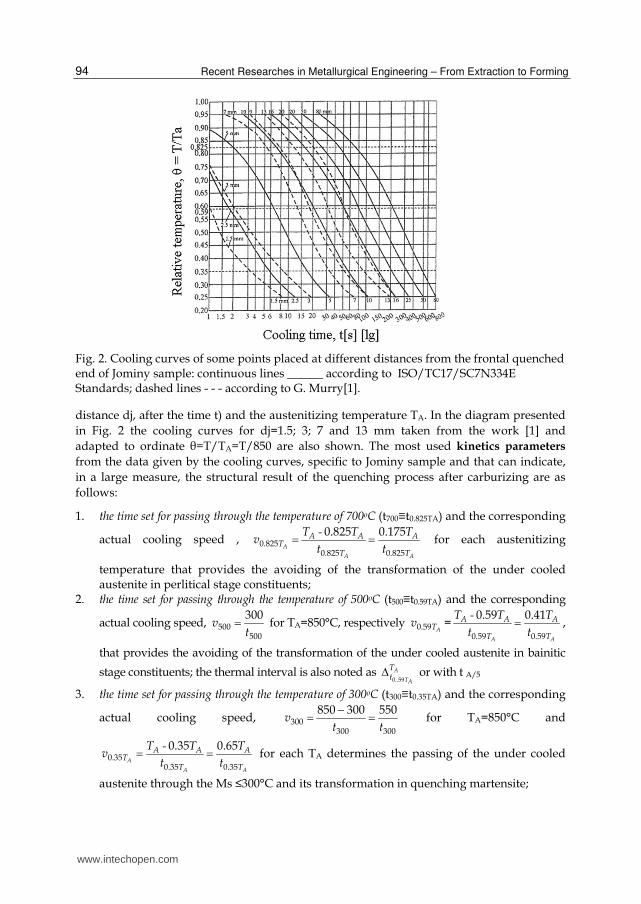
Fig. 2. Cooling curves of some points placed at different distances from the frontal quenched end of Jominy sample: continuous lines ______ according to ISO/TC17/SC7N334E Standards; dashed lines - - - according to G. Murry[1].

distance dj, after the time t) and the austenitizing temperature TA. In the diagram presented

in Fig. 2 the cooling curves for dj=1.5; 3; 7 and 13 mm taken from the work [1] and

adapted to ordinate θ=T/TA=T/850 are also shown. The most used kinetics parameters

from the data given by the cooling curves, specific to Jominy sample and that can indicate,

in a large measure, the structural result of the quenching process after carburizing are as

follows:

1. the time set for passing through the temperature of 700oC (t700≡t0.825TA) and the corresponding

actual cooling speed , -

A

A A

A A AT

T T

T T Tv

t t0.825

0.825 0.825

0.825 0.175 for each austenitizing

temperature that provides the avoiding of the transformation of the under cooled austenite in perlitical stage constituents;


actual cooling speed, vt

500500

300 for TA=850°C, respectively ATv0.59 =

-

A A

A A A

T T

T T T

t t0.59 0.59

0.59 0.41 ,

that provides the avoiding of the transformation of the under cooled austenite in bainitic

stage constituents; the thermal interval is also noted as A

TA

Tt0..59

or with t A/5


actual cooling speed, vt t

300300 300

850 300 550 for TA=850°C and

- A

A A

A A AT

T T

T T Tv

t t0.35

0.35 0.35

0.35 0.65 for each TA determines the passing of the under cooled

austenite through the Ms ≤300°C and its transformation in quenching martensite;

www.intechopen.com


95

4. the time interval t t t850300 300 850 for TA=850°C, respectively A

A

TTt0.825

0.35 , for each TA and

the average cooling speed of austenite in these temperature intervals ,

vt t

850300 850 850

300 300

850 300 550 , for TA=850°C, respectively v-

A

A A

A

T A AT T

T

T T

t

0.8250.35 0.825

0.35

0.825 0.35 for

each TA.

These parameters provide the cooling of the under cooled austenite in the range of MS-Mf

and its transformation in quenching martensite. The above mentioned kinetic parameters

are determined for each cooling curve, corresponding to a certain distance dJ [mm] from the

frontal quenched end of the Jominy test sample (Fig. 3).

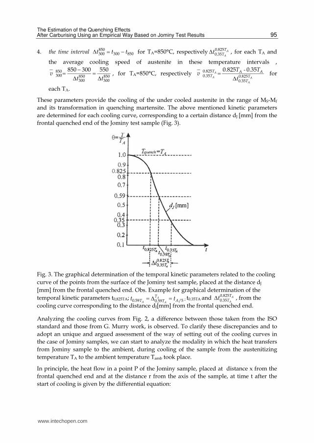
Fig. 3. The graphical determination of the temporal kinetic parameters related to the cooling

curve of the points from the surface of the Jominy test sample, placed at the distance dJ

[mm] from the frontal quenched end. Obs. Example for graphical determination of the

temporal kinetic parameters t0,825TA; A

A A

TT ATt t0.59 /50.59 ; t0.35TA and A

A

TTt0.825

0.35 , from the

cooling curve corresponding to the distance dJ[mm] from the frontal quenched end.

Analyzing the cooling curves from Fig. 2, a difference between those taken from the ISO

standard and those from G. Murry work, is observed. To clarify these discrepancies and to

adopt an unique and argued assessment of the way of setting out of the cooling curves in

the case of Jominy samples, we can start to analyze the modality in which the heat transfers

from Jominy sample to the ambient, during cooling of the sample from the austenitizing

temperature TA to the ambient temperature Tamb took place.

In principle, the heat flow in a point P of the Jominy sample, placed at distance x from the

frontal quenched end and at the distance r from the axis of the sample, at time t after the

start of cooling is given by the differential equation:

www.intechopen.com


96

x r t

P t r x t

TQ Q r

r r r

( , , )( ) ( , , )

(1)

this can be solved in the following univocity conditions:

a. initial condition: T(x,0)=TA ; b. boundary conditions of first order: T(0,t) =T water jet (on the water cooled surface)

T(x,t)=Tamb(along the cylinder generator) c. boundary conditions of second order defined by the specific heat flux through the

frontal cooled surface and through the external cylindrical surface cooled in air, which are proportional with the negative temperature gradients:

t

F

TW

x

(0, ) , respectivelyx t

cil

TW

x

( , ) (2)

The heat loss during sample cooling takes place by means of three mechanisms:

- conduction – at the contact interface between cooling water and direct cooled surface,

the heat loss value being a function of time:

W t q t( ) ( ) (3a)

- convection - of the ambient air, the heat loss value being a function of the T(x,t)-Tamb difference

(x,t) ambW(t) T T (3b)

where is the convection heat transfer coefficient:

- radiation - from the cylindrical surface:

x t ambW t T T4 4( , )( ) (3c)

where is the radiation constant, ;

is the emissivity coefficient of the sample surface;

82 4

J5.67.10

m sK

The solving of the differential equation (1) lead to a solution representing the general form of

the cooling curves equations of points placed at the distance x from the frontal quenched end:

x t amb A amb

cT T T T t

x( , ) ( )exp

(4)

where the parameter c has speed dimensions (m/s), and the rapport c/x is a constant on

which the temporary (instantaneous) cooling speed has a linear dependency:

amb

T cv T T

t x

(5)

www.intechopen.com


97

To simplify the analysis, without introducing further errors, can be admitted that Tamb~0

and noting T(x,t)=TS (the current surface temperature) and TS/TA=θ (the relative surface

temperature), the final solution can be written as:

ct

xe (6)

The solution (6) makes the direct connection between the relative temperature θ and time t,

values that represent the coordinates in which are drawn the cooling curves of the points

(planes) placed at the distance x from the frontal quench end of the Jominy sample.

In the work [2] the using of the relation (4) is exemplified in the case of Jominy samples

austenitized at TA=1050oC, for which the cooling curves of the points placed at the distances

x=1, 10, 20 and 40 mm from the frontal quench end (Fig.4) were drawn and on which the

ordinate referring to the relative temperature θ=T/1050 and also the ISO and Murry cooling

curves for distances x = 1.5 mm (Murry), 9mm (Murry),10 mm (Murry), 20 mm (ISO and

Murry) and 40 mm (Murry) were also drawn.

Using data taken from continuous curves presented in Fig.4 and replacing the notation x

which represents the distance from the frontal quenched end of Jominy sample with E, the

value of parameter c (from eq. 6) has found as c = 0.28, so that eq.(6) of cooling curves will

get a particular form (7) and the inverse function, t = f (θ) will have the expression (eq.8)

0.28

tEe

(7)

- t E8.244 lg (8)

On the other hand, from Fig. 4 it can be seen that between the aspect of the actual cooling curves experimentally determined by Murry and ISO and that obtained by calculation, using the relations (7) and (8), there are differences which are substantially and simultaneously amplifying with the decreasing of the relative temperature θ. In conclusion, we can say that the theoretical analysis presented above is incomplete in that it fails to consider some effects of interaction between the types of heat loss during cooling of the Jominy samples.

Taking into account the higher matching of the Murry curves to theoretical curves, were

mathematically processed the data provided by Murry curves and was noted that these are

best described also by an exponential function, having the general form t=aEb, and the

particular form as:

t aE1.41 (9)

where the parameter a depends on θ also by means of an exponential relation:

- a 2.40,2 (10)

In conclusion, the relations describing the dependencies t f E( , ) - eq.(8) and f t E( , ) -

eq. (7), will have the following particularly forms:

www.intechopen.com


98

- Et E2.4 1.41

( , ) 0.2 (11)

-E t E t0.588 0.416

( , ) 0.51 (12)

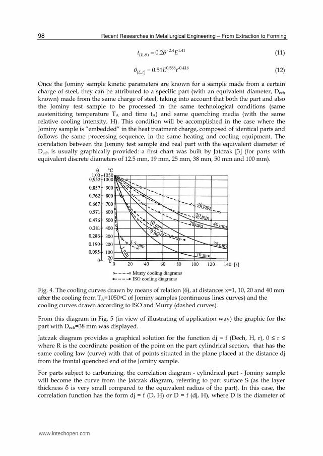
Once the Jominy sample kinetic parameters are known for a sample made from a certain charge of steel, they can be attributed to a specific part (with an equivalent diameter, Dech known) made from the same charge of steel, taking into account that both the part and also the Jominy test sample to be processed in the same technological conditions (same austenitizing temperature TA and time tA) and same quenching media (with the same relative cooling intensity, H). This condition will be accomplished in the case where the Jominy sample is “embedded” in the heat treatment charge, composed of identical parts and follows the same processing sequence, in the same heating and cooling equipment. The correlation between the Jominy test sample and real part with the equivalent diameter of Dech is usually graphically provided: a first chart was built by Jatczak [3] (for parts with equivalent discrete diameters of 12.5 mm, 19 mm, 25 mm, 38 mm, 50 mm and 100 mm).

Fig. 4. The cooling curves drawn by means of relation (6), at distances x=1, 10, 20 and 40 mm after the cooling from TA=1050oC of Jominy samples (continuous lines curves) and the cooling curves drawn according to ISO and Murry (dashed curves).

From this diagram in Fig. 5 (in view of illustrating of application way) the graphic for the part with Dech=38 mm was displayed.

Jatczak diagram provides a graphical solution for the function dj = f (Dech, H, r), 0 ≤ r ≤

where R is the coordinate position of the point on the part cylindrical section, that has the

same cooling law (curve) with that of points situated in the plane placed at the distance dj

from the frontal quenched end of the Jominy sample.

For parts subject to carburizing, the correlation diagram - cylindrical part - Jominy sample will become the curve from the Jatczak diagram, referring to part surface S (as the layer thickness δ is very small compared to the equivalent radius of the part). In this case, the correlation function has the form dj = f (D, H) or D = f (dj, H), where D is the diameter of

www.intechopen.com


99

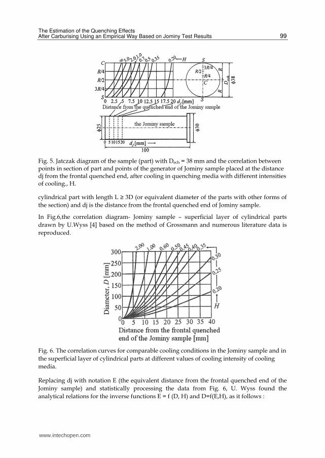
Fig. 5. Jatczak diagram of the sample (part) with Dech = 38 mm and the correlation between points in section of part and points of the generator of Jominy sample placed at the distance dj from the frontal quenched end, after cooling in quenching media with different intensities of cooling., H.

cylindrical part with length L ≥ 3D (or equivalent diameter of the parts with other forms of

the section) and dj is the distance from the frontal quenched end of Jominy sample.

In Fig.6,the correlation diagram- Jominy sample – superficial layer of cylindrical parts

drawn by U.Wyss [4] based on the method of Grossmann and numerous literature data is

reproduced.

Fig. 6. The correlation curves for comparable cooling conditions in the Jominy sample and in

the superficial layer of cylindrical parts at different values of cooling intensity of cooling

media.

Replacing dj with notation E (the equivalent distance from the frontal quenched end of the

Jominy sample) and statistically processing the data from Fig. 6, U. Wyss found the

analytical relations for the inverse functions E = f (D, H) and D=f(E,H), as it follows :

www.intechopen.com


100

- For a cooling intensity of H=0.25, corresponding to low agitated oil:

ED E(1.27 0.0042 )0.25

- DE D(0.755 0.0003 )0.25 (13)

- For a cooling intensity of H=0.35, corresponding to average agitated oil:

ED E(1.52 0.0028 )0.35

- DE D(0.649 0.0001 )0.35 (14)

- For a cooling intensity of H=0.45, corresponding to intensive agitated oil:

D E1.7550.45 E D0.57

0.45 (15)

- For a cooling intensity of H=0.60, corresponding to strong agitated oil:

D E20.60 E D0.50

0.60 (16)

- For a cooling intensity of H=1.00 , corresponding to low agitated water:

ED E(2 0.03 )1.00

- DE D(0.47 0.00015 )1.00 (17)

The values of cooling intensity, H, shown above, are suitable for quenching oil used at normal temperatures (50 ~ 80 °C) and with different degrees of agitation (of oil and/or parts) in a relatively wide range, starting from absence of agitation (H=0.25) to strong agitation (H=0.6), or a shower or pressure jet oil (H = 1.00), this last situation being equivalent for low agitated cooling water at 20 ° C, .

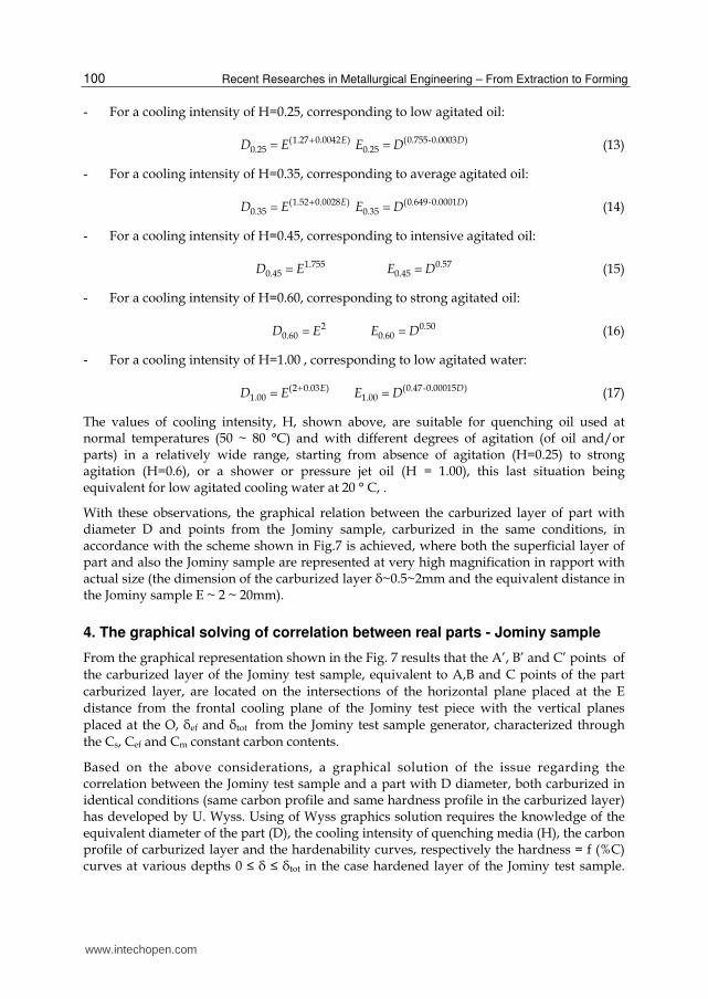
With these observations, the graphical relation between the carburized layer of part with diameter D and points from the Jominy sample, carburized in the same conditions, in accordance with the scheme shown in Fig.7 is achieved, where both the superficial layer of part and also the Jominy sample are represented at very high magnification in rapport with actual size (the dimension of the carburized layer δ~0.5~2mm and the equivalent distance in the Jominy sample E ~ 2 ~ 20mm).

4. The graphical solving of correlation between real parts - Jominy sample

From the graphical representation shown in the Fig. 7 results that the A’, B’ and C’ points of

the carburized layer of the Jominy test sample, equivalent to A,B and C points of the part

carburized layer, are located on the intersections of the horizontal plane placed at the E

distance from the frontal cooling plane of the Jominy test piece with the vertical planes

placed at the O, δef and δtot from the Jominy test sample generator, characterized through

the Cs, Cef and Cm constant carbon contents.

Based on the above considerations, a graphical solution of the issue regarding the correlation between the Jominy test sample and a part with D diameter, both carburized in identical conditions (same carbon profile and same hardness profile in the carburized layer) has developed by U. Wyss. Using of Wyss graphics solution requires the knowledge of the equivalent diameter of the part (D), the cooling intensity of quenching media (H), the carbon profile of carburized layer and the hardenability curves, respectively the hardness = f (%C) curves at various depths 0 ≤ δ ≤ δtot in the case hardened layer of the Jominy test sample.

www.intechopen.com


101

Fig. 7. The correlation scheme between part with equivalent diameter D and the Jominy

sample, carburized in identical conditions.

The scheme of Wyss's graphical solution is represented in detail in Fig.8 for certain parts with the equivalent diameter D = 35 mm, made of case hardened steel with composition 0.16% C, 1%Mn and 1%Cr that were carburized at Cs = 0.8% and quenched in hot oil with average agitation (cooling intensity of H = 0.35).

The information sources used by Wyss in developing of the scheme shown in Fig. 8 were the

following:

- the D=f(dj) dependence for H=0.35, has been taken from Fig. 6; - the carbon profile curve has been experimentally plotting by means of sequential

corrections of the case hardened layer of a part with dimensions of Φ35 x105 mm;

www.intechopen.com


102

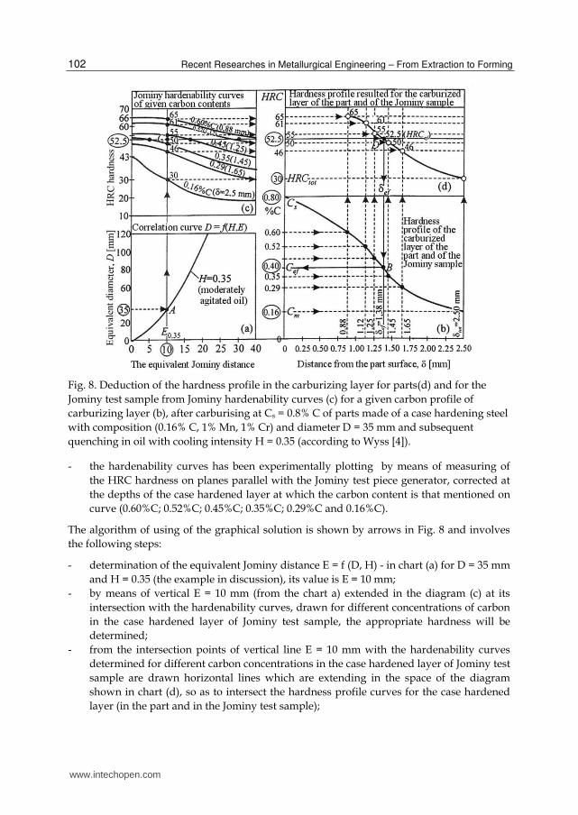
Fig. 8. Deduction of the hardness profile in the carburizing layer for parts(d) and for the

Jominy test sample from Jominy hardenability curves (c) for a given carbon profile of

carburizing layer (b), after carburising at Cs = 0.8% C of parts made of a case hardening steel

with composition (0.16% C, 1% Mn, 1% Cr) and diameter D = 35 mm and subsequent

quenching in oil with cooling intensity H = 0.35 (according to Wyss [4]).

- the hardenability curves has been experimentally plotting by means of measuring of

the HRC hardness on planes parallel with the Jominy test piece generator, corrected at

the depths of the case hardened layer at which the carbon content is that mentioned on

curve (0.60%C; 0.52%C; 0.45%C; 0.35%C; 0.29%C and 0.16%C).

The algorithm of using of the graphical solution is shown by arrows in Fig. 8 and involves

the following steps:

- determination of the equivalent Jominy distance E = f (D, H) - in chart (a) for D = 35 mm

and H = 0.35 (the example in discussion), its value is E = 10 mm;

- by means of vertical E = 10 mm (from the chart a) extended in the diagram (c) at its

intersection with the hardenability curves, drawn for different concentrations of carbon

in the case hardened layer of Jominy test sample, the appropriate hardness will be

determined;

- from the intersection points of vertical line E = 10 mm with the hardenability curves

determined for different carbon concentrations in the case hardened layer of Jominy test

sample are drawn horizontal lines which are extending in the space of the diagram

shown in chart (d), so as to intersect the hardness profile curves for the case hardened

layer (in the part and in the Jominy test sample);

www.intechopen.com


103

- in the diagram (b) the horizontals lines corresponding to the hardenability curves from the diagram(c) will be plotted and the points of intersection with the carbon profile curve will be determined; from these points, vertical lines extending in the space of the diagram (d) are drawn and cross the horizontals plotted in an earlier stage (from the intersection points of the vertical E = 10 mm (diagram (a)) with the hardenability curves drawn for different carbon concentrations in the case hardened layer (diagram (c)); the intersection points belong to the hardness profile curve available for the existing space diagram (d). The point D in the diagram (d) in which the hardness profile curve crosses the horizontal corresponding to HRCef hardness has the abscise corresponding to the effective depth δef (in the example discussed, for HRCef = 52.5 results δef=1.38 mm);

- from the crossing point D, the vertical line which will meet the carbon profile curve at point B of which horizontal corresponds to the actual carbon content, Cef (for example the analysis made for δef = 1.38 mm results Cef = 0.4% C).

5. Essay regarding the analytical solving of the real parts-Jominy sample correlation

The above graphical solution can be transformed into an analytical solution if the equations

of the following curves are available:

a. E = f (D, H) curve; b. C = f (δ) carbon profile curve; c. Jominy hardenability curve, HRC = f (C, d)

a. For the equation (a) it can be started from the mathematical processing of the Wyss

particular relations no (13) ~ (17) in order to their generalization. The performed attempts

lead to two different types of generalized relations, applicable with satisfactory accuracy on

different values ranges for the H, D and E variables:

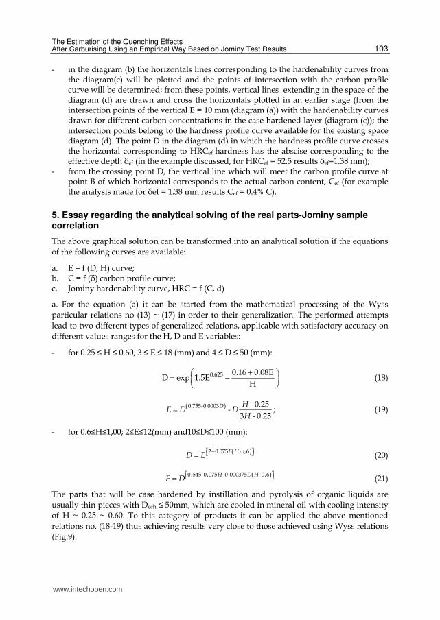
- for 0.25 ≤ H ≤ 0.60, 3 ≤ E ≤ 18 (mm) and 4 ≤ D ≤ 50 (mm):

0.625 0.16 0.08ED exp 1.5E

H

(18)

- --

-

D HE D D

H

0.755 0.0003 0.25

3 0.25 ; (19)

- for 0.6≤H≤1,00; 2≤E≤12(mm) and10≤D≤100 (mm):

-E H o

D E2 0.075 ,6 (20)

- - -H D H

E D0,545 0,075 0,000375 0,6 (21)

The parts that will be case hardened by instillation and pyrolysis of organic liquids are

usually thin pieces with Dech ≤ 50mm, which are cooled in mineral oil with cooling intensity

of H ~ 0.25 ~ 0.60. To this category of products it can be applied the above mentioned

relations no. (18-19) thus achieving results very close to those achieved using Wyss relations

(Fig.9).

www.intechopen.com


104

Fig. 9. Comparison between the effects of using of the Wyss particular relations and the relation no.(19) [5].

b. For the equation of the carbon profile curve (b), can be used the expression of criterial

solution of the diffusion equation obtained through solving in the boundary conditions of III

order – ec. 23, written under the form:

Cδ=Cm+θ(Cs-Cm) (22)

where Cδ represents the carbon content measured at the δ depth in rapport with the surface

at the case hardening end; Cm represents the carbon content of the non – case hardened core

and Cs is the surface carbon content at the end of case hardening.

mk k

S m k k

C Cerfc h Dt h erfc h Dt

C C Dt Dt

2exp .2 2

(23)

where tk represents the carburising time, h=K/D, represents the relative coefficient of mass

transfer, K- is the global coefficient of mass transfer in the case hardening medium; D - the

diffusion coefficient of carbon in austenite.

c. For the Jominy hardenability curbes (c) have been deduced by E. Just [6] several regression equations having the general form:

d i iJ A C Bd C Dd E d k c FN G2 (24)

where C is the carbon content of steel, [% C], ci- content of alloying elements in steel [% E],

d - distance from the quenched end of the Jominy test sample [mm], N - the ASTM score of

the austenitic grain; A, B, D, E, F and G are the regression coefficients and Jd the HRC

hardness at the d distance in the Jominy test sample.

Replacing the d distance with the equivalent Jominy distance E and Jd with HRC(E), can be

retained the following three Just formulas, used also in other literature [4] - [7]:

www.intechopen.com


105

- - -EHRC C E C E E Mn Cr Ni Mo298 0.01 1.79 19 19 20 6.4 34 7 (25)

- 0 - - -EHRC C E C E E Si Mn Cr Ni Mo N288 .0053 1.32 15.8 5 16 19 6.3 35 0.82 2 (26)

These relations are valid for the following limits of carbon and alloying elements

concentrations: 0.08%≤C≤0.56%; Si≤3.8%; Mn≤1.88%; Cr≤1.97%; Ni≤8.94%; Mo≤0.53% and

for an austenitic score in the limits 1.5≤N≤11

- -EHRC C E E Mn Cr Ni Mo102 1.102 15,47 21 22 7 33 16 (27)

relation valid for the steels with 0.25≤%C≤0.60 and with the admissible alloying elements

concentrations given by relations no. (25-26).The three relations produce results significantly

closer each to another and also very close to those provided by the graphical dependencies

for a series of German steels presented in the work [7]. Therefore, it was adopted for

explaining of the hardenability curve the relation no. (27) is written as:

- -EHRC C E E S102 1.102 15.47 16 (28)

where S Mn Cr Ni Mo21 22 7 33 (29)

In connection with the application of relation (ec.28), have to be specified that the HRC(E)

may not exceed a certain maximum value, which is corresponding to the hardness of the

fully martensitic structure (HRC100%M), dependent in turn on the carbon content of

martensite (austenite which is totally transformed into quenching martensite). To calculate

the maximum hardness E. Just proposed the relation:

MHRC C0,7100 29 51 (30)

which is applicable to steels with carbon content in the limits 0.1%≤C≤0.6%.

Besides relation (30), in the speciality literature are presented also other relations, including

the most complex relation specified in ASTM A 255 / 1989 with the polynomial expression:

- -MHRC C C C C C2 3 4 5100 35.395 6.99 312.33 821.74 1015.48 538.34 (31)

applicable to steel with C≤0.7%.

On the other hand, in the technical literature are published more data under graphical form,

where are presented the hardnesses of quenching structures, experimentally determined,

depending on the carbon content and the proportion of martensite in the hardening

structure (Table 2). The charts from where the data from Table 2 were taken, suggest that the

hardness of the quenching structures increases with carbon content in steel after curves that

have the tendency to be closed to some limits values at high carbon contents. Starting from

this observation, it was considered that the most appropriate analytical expression of the

hardness dependence on carbon content can be obtained by using a prognosis function with

tendency of "saturation".

www.intechopen.com


106

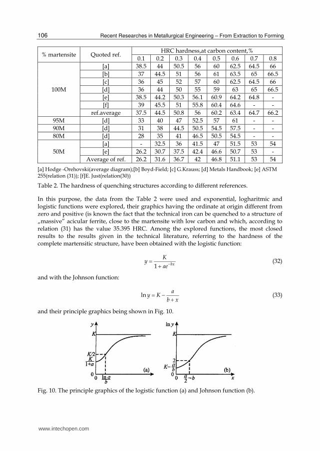
% martensite Quoted ref. HRC hardness,at carbon content,%

0.1 0.2 0.3 0.4 0.5 0.6 0.7 0.8

100M

[a] 38.5 44 50.5 56 60 62.5 64.5 66

[b] 37 44.5 51 56 61 63.5 65 66.5

[c] 36 45 52 57 60 62.5 64.5 66

[d] 36 44 50 55 59 63 65 66.5

[e] 38.5 44.2 50.3 56.1 60.9 64.2 64.8 -

[f] 39 45.5 51 55.8 60.4 64.6 - -

ref.average 37.5 44.5 50.8 56 60.2 63.4 64.7 66.2

95M [d] 33 40 47 52.5 57 61 - -

90M [d] 31 38 44.5 50.5 54.5 57.5 - -

80M [d] 28 35 41 46.5 50.5 54.5 - -

50M

[a] - 32.5 36 41.5 47 51.5 53 54

[e] 26.2 30.7 37.5 42.4 46.6 50.7 53 -

Average of ref. 26.2 31.6 36.7 42 46.8 51.1 53 54

[a] Hodge -Orehovski(average diagram);[b] Boyd-Field; [c] G.Krauss; [d] Metals Handbook; [e] ASTM 255(relation (31)); [f]E. Just(relation(30))

Table 2. The hardness of quenching structures according to different references.

In this purpose, the data from the Table 2 were used and exponential, logharitmic and logistic functions were explored, their graphics having the ordinate at origin different from zero and positive (is known the fact that the technical iron can be quenched to a structure of „massive” acicular ferrite, close to the martensite with low carbon and which, according to relation (31) has the value 35.395 HRC. Among the explored functions, the most closed results to the results given in the technical literature, referring to the hardness of the complete martensitic structure, have been obtained with the logistic function:

bx

Ky

ae1 (32)

and with the Johnson function:

a

y Kb x

ln (33)

and their principle graphics being shown in Fig. 10.

Fig. 10. The principle graphics of the logistic function (a) and Johnson function (b).

www.intechopen.com


107

For the hardness of the complete martensitic structure, the two functions mentioned above have the particular forms:

-

MHRCC

100

70

1 1.35exp( 4,24 ) (34)

100M

0.36HRC exp 4.55

0.27 C

(35)

The formulas no. (34) and (35) give results very close each to another and also close to the experimental data referring to steels with carbon content in the limits 0.1~0.8%.

Furthermore the Johnson function can be used with satisfactory results also for the calculation of the hardness of the quenched layers in which the martensite proportion decreases to 50%.

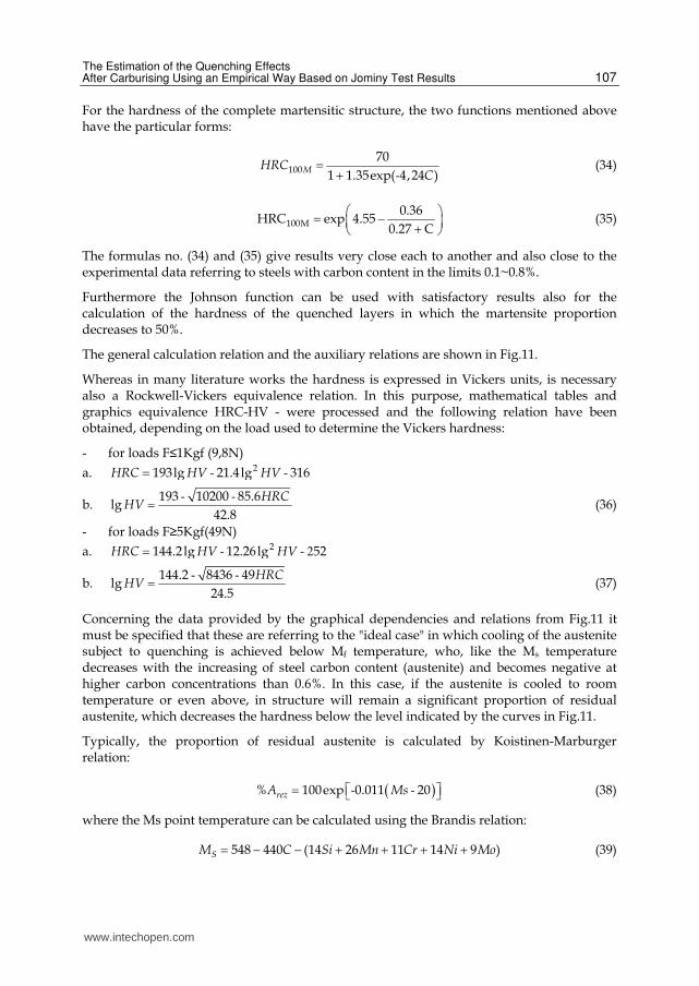
The general calculation relation and the auxiliary relations are shown in Fig.11.

Whereas in many literature works the hardness is expressed in Vickers units, is necessary also a Rockwell-Vickers equivalence relation. In this purpose, mathematical tables and graphics equivalence HRC-HV - were processed and the following relation have been obtained, depending on the load used to determine the Vickers hardness:

- for loads F≤1Kgf (9,8N)

a. - -HRC HV HV2193lg 21.4lg 316

b. - - HRC

HV193 10200 85.6

lg42.8

(36)

- for loads F≥5Kgf(49N)

a. - - 2HRC HV HV2144.2 lg 12.26lg 52

b. - - HRC

HV144.2 8436 49

lg24.5

(37)

Concerning the data provided by the graphical dependencies and relations from Fig.11 it must be specified that these are referring to the "ideal case" in which cooling of the austenite subject to quenching is achieved below Mf temperature, who, like the Ms temperature decreases with the increasing of steel carbon content (austenite) and becomes negative at higher carbon concentrations than 0.6%. In this case, if the austenite is cooled to room temperature or even above, in structure will remain a significant proportion of residual austenite, which decreases the hardness below the level indicated by the curves in Fig.11.

Typically, the proportion of residual austenite is calculated by Koistinen-Marburger relation:

- -rezA Ms% 100exp 0.011 20 (38)

where the Ms point temperature can be calculated using the Brandis relation:

SM C Si Mn Cr Ni Mo548 440 (14 26 11 14 9 ) (39)

www.intechopen.com


108

Fig. 11. The hardness of the quenching structures depending on carbon content of steel (austenite) and on the martensite proportion from the structure; continuous curves______ drawn up with Johnsonunction; dashed curves _ _ _ _ _ drawn up with logistical function.

Decreasing of hardness caused by the presence of residual austenite can be calculated with the relation:

a. rez

rez

AHV

A

%

0.10 0.015 % (40)

derived from data provided by G. Krauss for hardnesses of fully martensitic structures (at

cooling under the temperature corresponding to the end of martensitic transformation - Mf)

and the structures formed by martensite and residual austenite (at cooling to room

temperature). If the hardness of carburized layer is measured in Rockwell units the

indicative relation can be used:

b. rez

rez

AHRC

A

%

1 0.2 % (41)

Returning to the analytical solution of the correlation between Jominy sample and real parts,

which should finally allow to draw the hardness curve of the carburized and quenched

www.intechopen.com


109

layer, is noted that this solution is materialized in a mathematical model of post carburising

quenching, whose solving algorithm is based on knowing of the initial data referring to the

following independent variables:

a. chemical composition of steel, respectively the alloying factor;

S Mn Cr Ni Mo21 22 7 33

b. the geometry of parts subject to carburising, respectively the equivalent diameter Dech;

c. the cooling intensity of the quenching medium, respectively the Grossmann (H) relative

cooling intensity;

d. the requested effective hardness (HRCef);

e. the requested effective case depth(δef).

Starting from this initial data, the algorithm for determining of the hardness curve of

carburized and quenched layer will require the following sequence of steps:

Step I taking into account the geometry of parts subject to processing, the equivalent

diameter Dech is calculated with one of the equivalence relations mentioned in Fig.1.

Step II taking into account Dech and h, is calculated the equivalent distance E from the

frontal quenched end of the Jominy sample by means of the relation (19) , written under the

form:

ech0.755 0.0003D

echech

H 0.25E D D

3H 0.25

(42)

Step III taking into account E and S and giving to the hardness the value HRCef , can be

calculated the effective carbon content Cef by means of relation (28), written under the form:

- -ef efHRC C E E S102 1.1 15.47 16 (43)

which lead to the relation:

2

efef

HRC 16 S 15.47 E 1.1EC

102

(44)

In the technical literature and in industrial practice of carburising followed by quenching,

for the actual hardness value is used most frequently HRCef = 52.5 (ie HVef=550).Using this

value, the equation (44) takes the following particular form:

2

ef52.5HRC(550HV)

68.5 S 15.47 E 1.1EC

102

(45)

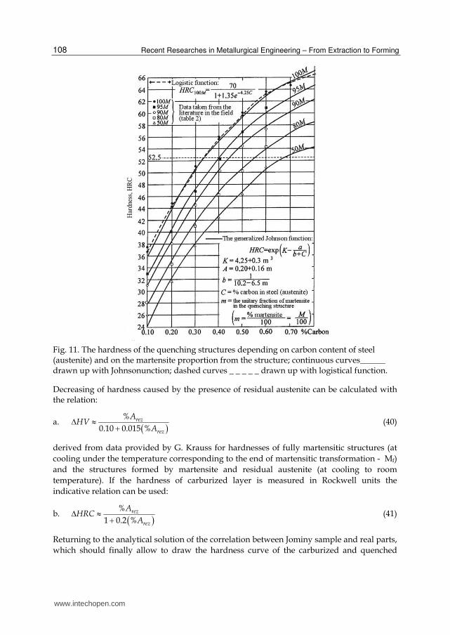
U.Wyss had drawn the curves (parabola) ef HRCC f E S52.5 ( , ) for several German case

hardening steels (Fig.12) with the average chemical composition (according to DIN-tab.3),

without mentioning of the calculation formula or the effective values of the alloying factors S.

www.intechopen.com


110

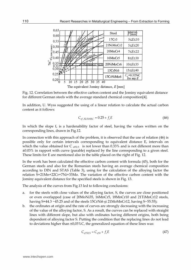
Fig. 12. Correlation between the effective carbon content and the Jominy equivalent distance for different German steels with the average standard chemical composition[4].

In addition, U. Wyss suggested the using of a linear relation to calculate the actual carbon content as it follows:

ef HRC cC f E,52.5 0.25 (46)

In which the slope fc is a hardenability factor of steel, having the values written on the corresponding lines, drawn in Fig.12.

In connection with this approach of the problem, it is observed that the use of relation (46) is possible only for certain intervals corresponding to equivalent distance E, intervals on which the value obtained for C ef52.5 is not lower than 0.33% and is not different more than ±0.03% in rapport with curve (parable) replaced by the line corresponding to a given steel. These limits for E are mentioned also in the table placed on the right of Fig. 12.

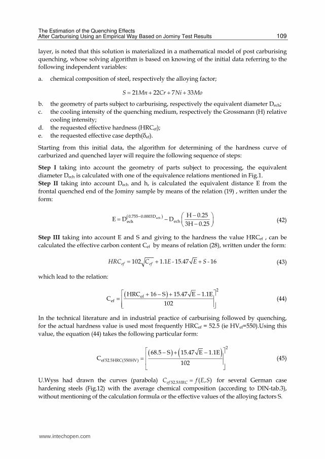
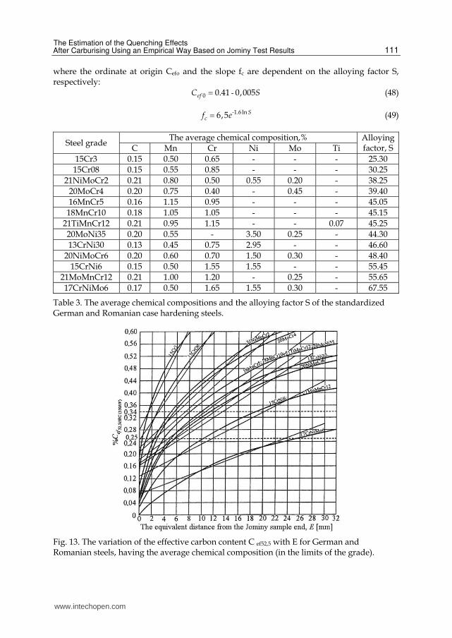
In the work has been calculated the effective carbon content with formula (45), both for the German steels and also for the Romanian steels having an average chemical composition according to DIN and STAS (Table 3), using for the calculation of the alloying factor the relation S=21Mn+22Cr+7Ni+33Mo. The variation of the effective carbon content with the Jominy equivalent distance for the specified steels is shown in Fig. 13.

The analysis of the curves from Fig.13 led to following conclusions:

a. for the steels with close values of the alloying factor, S, the curves are close positioned or even overlapped (case of 20MoNi35, 16MnCr5, 18MnCr10 and 21TiMnCr12 steels, having S=44.3 ~45.25 and of the steels 15CrNi6 şi 21MoMnCr12, having S~55.55);

b. the ordinates at origin and the rate of curves are strongly decreasing with the increasing of the value of the alloying factor, S. As a result, the curves can be replaced with straight lines with different slope, but also with ordinates having different origins, both being dependent of alloying factor S. Putting the condition that the replacing lines do not lead to deviations higher than ±0,03%C, the generalized equation of these lines was:

ef ef cC C f E52.5 0 (47)

www.intechopen.com


111

where the ordinate at origin Cefo and the slope fc are dependent on the alloying factor S, respectively:

-efC S0 0.41 0,005 (48)

- Scf e 1.6 ln6,5 (49)

Steel grade The average chemical composition,% Alloying

factor, S C Mn Cr Ni Mo Ti

15Cr3 0.15 0.50 0.65 - - - 25.30

15Cr08 0.15 0.55 0.85 - - - 30.25

21NiMoCr2 0.21 0.80 0.50 0.55 0.20 - 38.25

20MoCr4 0.20 0.75 0.40 - 0.45 - 39.40 16MnCr5 0.16 1.15 0.95 - - - 45.05

18MnCr10 0.18 1.05 1.05 - - - 45.15

21TiMnCr12 0.21 0.95 1.15 - - 0.07 45.25

20MoNi35 0.20 0.55 - 3.50 0.25 - 44.30

13CrNi30 0.13 0.45 0.75 2.95 - - 46.60

20NiMoCr6 0.20 0.60 0.70 1.50 0.30 - 48.40

15CrNi6 0.15 0.50 1.55 1.55 - - 55.45 21MoMnCr12 0.21 1.00 1.20 - 0.25 - 55.65

17CrNiMo6 0.17 0.50 1.65 1.55 0.30 - 67.55

Table 3. The average chemical compositions and the alloying factor S of the standardized German and Romanian case hardening steels.

Fig. 13. The variation of the effective carbon content C ef52,5 with E for German and Romanian steels, having the average chemical composition (in the limits of the grade).

www.intechopen.com


112

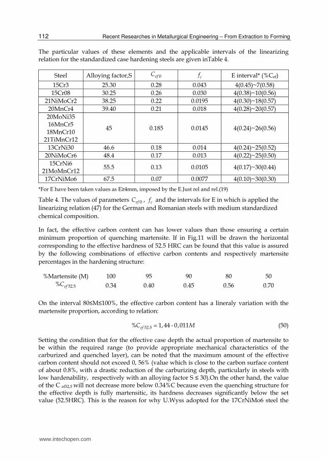
The particular values of these elements and the applicable intervals of the linearizing relation for the standardized case hardening steels are given inTable 4.

Steel Alloying factor,S efC 0 cf E interval* (%Cef)

15Cr3 25.30 0.28 0.043 4(0.45)~7(0.58)

15Cr08 30.25 0.26 0.030 4(0.38)~10(0.56)

21NiMoCr2 38.25 0.22 0.0195 4(0.30)~18(0.57)

20MnCr4 39.40 0.21 0.018 4(0.28)~20(0.57)

20MoNi35 16MnCr5

18MnCr10 21TiMnCr12

45 0.185 0.0145 4(0.24)~26(0.56)

13CrNi30 46.6 0.18 0.014 4(0.24)~25(0.52)

20NiMoCr6 48.4 0.17 0.013 4(0.22)~25(0.50)

15CrNi6 21MoMnCr12

55.5 0.13 0.0105 4(0.17)~30(0.44)

17CrNiMo6 67.5 0.07 0.0077 4(0.10)~30(0.30)

*For E have been taken values as E≥4mm, imposed by the E.Just rel and rel.(19)

Table 4. The values of parameters efC 0 , cf and the intervals for E in which is applied the

linearizing relation (47) for the German and Romanian steels with medium standardized

chemical composition.

In fact, the effective carbon content can has lower values than those ensuring a certain

minimum proportion of quenching martensite. If in Fig.11 will be drawn the horizontal

corresponding to the effective hardness of 52.5 HRC can be found that this value is assured

by the following combinations of effective carbon contents and respectively martensite

percentages in the hardening structure:

%Martensite (M) 100 95 90 80 50

efC 52.5% 0.34 0.40 0.45 0.56 0.70

On the interval 80≤M≤100%, the effective carbon content has a lineraly variation with the

martensite proportion, according to relation:

-efC M52.5% 1,44 0,011 (50)

Setting the condition that for the effective case depth the actual proportion of martensite to be within the required range (to provide appropriate mechanical characteristics of the carburized and quenched layer), can be noted that the maximum amount of the effective carbon content should not exceed 0, 56% (value which is close to the carbon surface content of about 0.8%, with a drastic reduction of the carburizing depth, particularly in steels with low hardenability, respectively with an alloying factor S ≤ 30).On the other hand, the value of the C ef52,5 will not decrease more below 0.34%C because even the quenching structure for the effective depth is fully martensitic, its hardness decreases significantly below the set value (52.5HRC). This is the reason for why U.Wyss adopted for the 17CrNiMo6 steel the

www.intechopen.com


113

amount Cef=0.33%, although in the carburized layer of steel, the information offered by relation (45) and Fig.13 shown that the hardness of 52.5HRC can be obtained even for the content of 0.17%C of core (at E=13 mm). In a subsequent paper [7], Weissohn and Roempler suggest as minimum value for the carbon content with the concentration of 0.28% (for which HRC100M~49.4, according to Fig.11). Adopting a value below that of the 0.34% could be justified for alloyed steel intended for carburising, due to the fact that alloyed martensite has a hardness higher with 1~2HRC than that of unalloyed steels.

In conclusion, for the calculation of the effective carbon content ( ef HRCC ,52.5 ) can be used the

linearizing relations (47-49),with supplementary restrictions:

a. E≥4mm

b. 0,28≤ ef HRCC ,52.5 ≤0.56% (respectively 100≥M≥80%)

Step IV Using Cef and δef , can be calculated the carburising time (t k) at isothermal carburising with a single cycle or the active carburising time (t k) ,respectively the diffusion time (tD), at carburising in two steps. The performing of this calculation supposes the knowing of thermal regime (tk,tD), the chemical regime(CpotK,Cpot D), the corresponding evaluation of the global mass transfer in the carburising medium (K); and the diffusion coefficient of carbon in austenite (D). Step V is based on knowing of the carbon profile and of the cooling law (curve) of the layer and has as final purpose the drawing of the layer hardness profile. The carbon profile can be determined after the step IV, and the cooling curve of layer can be drawn using the relation (11).

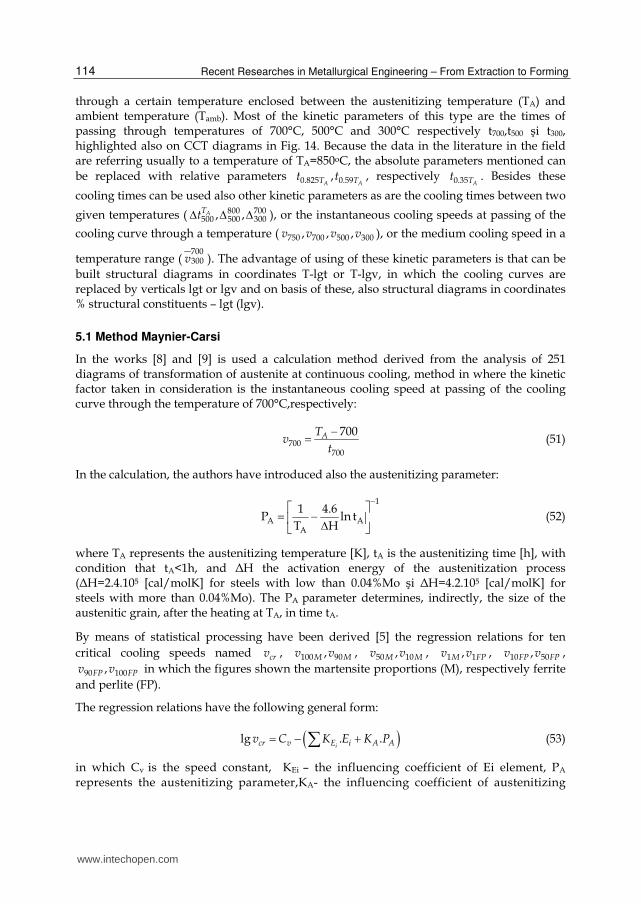
The most direct method for determining and drawing of the hardness profile consist in overlapping of the cooling curve of the case hardened layer on the transformation diagrams of continuous cooling of austenite (CCT diagrams) „of different steels” from the layer, steels with carbon content that decreases from surface to core. The method is illustrated in Fig.14, for the case where the diagrams for the austenite transformation, corresponding for three steels with different carbon content that will be carburized, are known:

a. with carbon content of core, Cm ; b. with effective carbon content, Cef ; c. with carbon content of surface, Cs

Because the temperatures corresponding to Ms point and the transformation ranges for the

three diagrams are placed differently in the plane T-t (at a lower position and to the right, as the carbon content increases), the intersections of these with the cooling curve led to different structures (decreasing of the proportions of bainite and increasing of the proportions of martensite), respectively with different hardnesses (HRCm< HRCef< HRC100M

For an accurate drawing of the hardness profile, is necessary to know a minimum number of 5-6 austenite transformation diagrams, corresponding to different carbon contents for a steel having in its chemical composition, all the other elements that are permanently accompanying and alloying elements with the same contents. But, this kind of technical "archive" is not currently available, even in the richest databases for the usual case-hardening steels. To overcome these difficulties can be used a hardness calculation method based on knowledge of chemical composition and of a kinetic parameter characteristic to cooling law of the case hardened layer. This parameter can be the cooling time at passing

www.intechopen.com


114

through a certain temperature enclosed between the austenitizing temperature (TA) and ambient temperature (Tamb). Most of the kinetic parameters of this type are the times of passing through temperatures of 700°C, 500°C and 300°C respectively t700,t500 şi t300, highlighted also on CCT diagrams in Fig. 14. Because the data in the literature in the field are referring usually to a temperature of TA=850oC, the absolute parameters mentioned can

be replaced with relative parameters A AT Tt t0.825 0.59, , respectively

ATt0.35 . Besides these

cooling times can be used also other kinetic parameters as are the cooling times between two

given temperatures ( ATt 800 700500 300500 , , ), or the instantaneous cooling speeds at passing of the

cooling curve through a temperature ( v v v v750 700 500 300, , , ), or the medium cooling speed in a

temperature range ( v700300 ). The advantage of using of these kinetic parameters is that can be

built structural diagrams in coordinates T-lgt or T-lgv, in which the cooling curves are replaced by verticals lgt or lgv and on basis of these, also structural diagrams in coordinates % structural constituents – lgt (lgv).

5.1 Method Maynier-Carsi

In the works [8] and [9] is used a calculation method derived from the analysis of 251 diagrams of transformation of austenite at continuous cooling, method in where the kinetic factor taken in consideration is the instantaneous cooling speed at passing of the cooling curve through the temperature of 700°C,respectively:

ATv

t700

700

700 (51)

In the calculation, the authors have introduced also the austenitizing parameter:

1

A AA

1 4.6P ln t

T H

(52)

where TA represents the austenitizing temperature [K], tA is the austenitizing time [h], with condition that tA<1h, and ΔH the activation energy of the austenitization process (ΔH=2.4.105 [cal/molK] for steels with low than 0.04%Mo şi ΔH=4.2.105 [cal/molK] for steels with more than 0.04%Mo). The PA parameter determines, indirectly, the size of the austenitic grain, after the heating at TA, in time tA.

By means of statistical processing have been derived [5] the regression relations for ten

critical cooling speeds named crv , M Mv v100 90, , M Mv v50 10, , M FPv v1 1, , FP FPv v10 50, ,

FP FPv v90 100, in which the figures shown the martensite proportions (M), respectively ferrite

and perlite (FP).

The regression relations have the following general form:

icr v E i A Av C K E K Plg . . (53)

in which Cv is the speed constant, KEi – the influencing coefficient of Ei element, PA represents the austenitizing parameter,KA- the influencing coefficient of austenitizing

www.intechopen.com


115

Fig. 14. Determination of the structure and hardness in different points in the carburized layer depth of the part and the Jominy sample. a) the CCT diagram of the not carburized core, with δ ≥ dtot and the core carbon content Cm; b) the CCT diagram of the layer point at depth def, with carbon content of Cef; c) the CCT diagram of the surface point of the part (δ = 0) with surface carbon content Cef; d) hardness profile of the carburized layer in the part and the Jominy sample.

parameter (of the austenitic grain size), and Ei represent the proportion of carbon, adding elements and alloying elements.

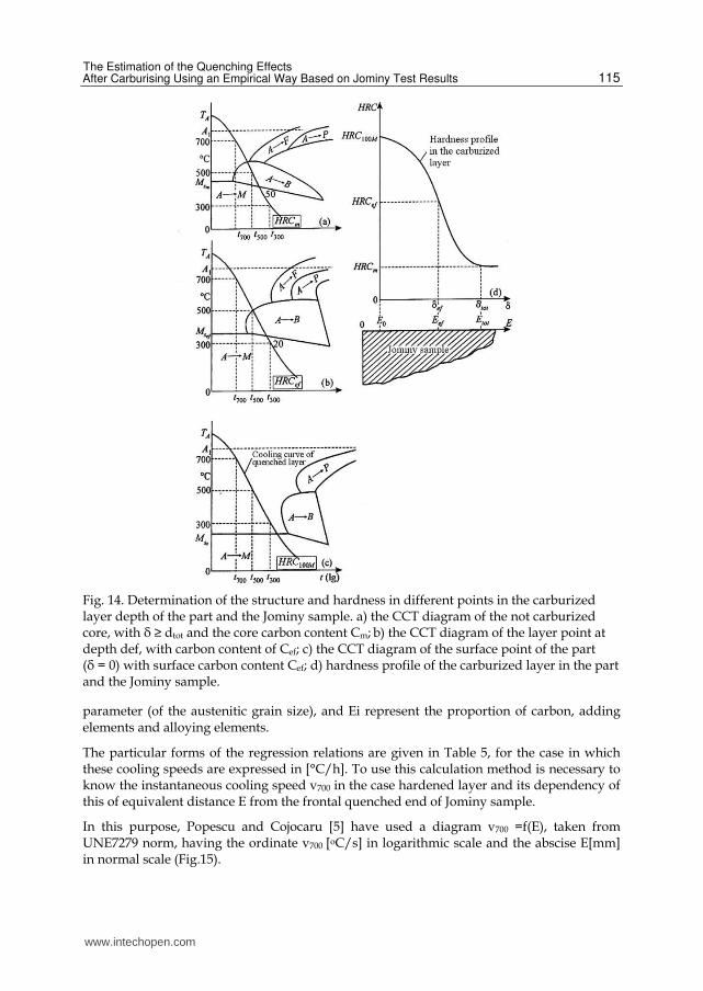
The particular forms of the regression relations are given in Table 5, for the case in which these cooling speeds are expressed in [°C/h]. To use this calculation method is necessary to know the instantaneous cooling speed v700 in the case hardened layer and its dependency of this of equivalent distance E from the frontal quenched end of Jominy sample.

In this purpose, Popescu and Cojocaru [5] have used a diagram v700 =f(E), taken from UNE7279 norm, having the ordinate v700 [oC/s] in logarithmic scale and the abscise E[mm] in normal scale (Fig.15).

www.intechopen.com


116

crv700

lg vC iEK for the element:

AK C Mn Ni Cr Mo

Mv100lg 9.81 4.62 0.78 0.41 0.80 0.66 0.0018

Mv90lg 8.76 4.04 0.86 0.36 0.58 0.97 0.0010

Mv50lg 8.20 3.00 0.79 0.57 0.67 0.94 0.0012

Mv10lg 9.80 3.90 -0.54 Mn ++2.45 Mn 0.46 0.50 1.16 0.0020

8.56 1.50 1.84 0.78 1.24 1.46 0.0020

FPv1lg 10.55 4.80 0.80 0.72 1.07 1.58 0.0026

FPv10lg 9.06 4.11 0.90 0.60 1.00 2.00 0.0013

FPv50lg 8.04 3.40 1.15 0.96 1.00 2.00 0.0007

FPv90lg 8.40 2.80 1.51 1.03 1.10 2.00 0.0014

FPv100lg 8.56 1.50 1.84 0.78 1.24 Mo2 0.0020

Table 5. The values of iv EC K, and AK ( PA in °C) from the regression relations (53)

Fig. 15. Dependency of the instantaneous cooling speed V700 on distance from the frontal quenched end of the Jominy sample (according to UNE 7279 [9].

The mathematical processing of data from this diagram shows that the function v700=f(E) has the form:

-v E 1.41700 500 [°C/s] (54)

-v E6 1.41700 1,8.10 [°C/h] (55)

The two relations offer results in accordance with data of Fig. 15, for 1.5≤E≤30mm.

Admitting that the austenitizing temperature, for the data shown in Fig.15 is TA=850°C

(which is not specified in the work [9], but is usually used in other works in the field), the

absolute instantaneous cooling speed v700 can be replaced with the relative speed v 0,825TA,

which will be calculated with the relation:

www.intechopen.com


117

-

A

A A

A A AT

T T

T T Tv

t t0,825

0.825 0.825

0.825 0.175 (56)

Combining this relation with the relation (11), in which θ=0.825, results:

-

AT Av T E 1,410.825 0.55 . (57)

For TA=850°C, relation (57) led to -v E 1.41700 468. , value which is very close to that given by

the relation(54), this is confirming also the validity of the relations (11) and (12).

Taking into account the critical speeds (calculated with the relations from Table 5) and the

carbon profile curve of the carburized layer allow the overlapping of the structural diagrams

at different carbon concentrations and taking into account the speed v700 (v0,825TA) of layer,

allow the positioning of the vertical of this speed in the space of the structural diagram and

the deriving of the proportions of the quenching constituents for each carbon content

(respectively for each depth) of carburized layer.

5.2 The Eckstein method

In paper [10], another drawing method of the hardness profile curve is provided, which is considered to be described as a complex exponential function as it follows:

b cEE SH H E e. . (58)

where SH is the surface hardness, respectively the martensite hardness which has the

superficial carbon content Cs, E is the equivalent Jominy distance in the depth of the case

hardened layer, and b and c are the coefficients dependent on the steel chemical composition.

For the calculation of the Jominy equivalent distance, the author provides the formula:

-A A AE t t t2 3/5 /5 /50.0877 0.761 0.0148 0.00012 (59)

where At /5 represents the cooling time from austenitizing temperature in view of cooling,

from 850°C, until 500°C.

The relation no.(59) is applicable for the case At s/5 42 (maximum values for parts with the

equivalent diameter D≤100mm, quenched in mineral oils with cooling intensity

0.25≤H≤0.60).

Due to fact that TA=850°C and Tcooling=500°C, results that the relative cooling temperature

has the value racire

5000.59

850 and the time At /5 can be replaced with time

ATt0.59 ,usable

for each austenitizing temperature in view of cooling, TA. With this specification, the

relation (11) can be used, from where, through the replacement E t( , ) 0.59 and through

variable changing, can be obtained the relation:

ATE t0,71

0,591.24 (60)

www.intechopen.com


118

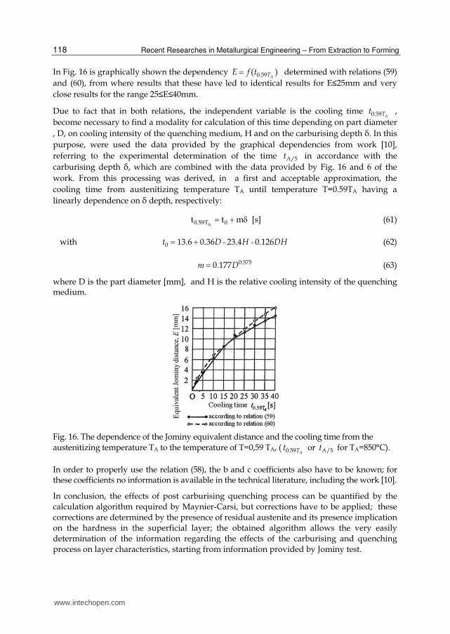
In Fig. 16 is graphically shown the dependency ATE f t0.59( ) determined with relations (59)

and (60), from where results that these have led to identical results for E≤25mm and very

close results for the range 25≤E≤40mm.

Due to fact that in both relations, the independent variable is the cooling time ATt0.59 ,

become necessary to find a modality for calculation of this time depending on part diameter

, D, on cooling intensity of the quenching medium, H and on the carburising depth δ. In this

purpose, were used the data provided by the graphical dependencies from work [10],

referring to the experimental determination of the time At /5 in accordance with the

carburising depth δ, which are combined with the data provided by Fig. 16 and 6 of the

work. From this processing was derived, in a first and acceptable approximation, the

cooling time from austenitizing temperature TA until temperature T=0.59TA having a

linearly dependence on δ depth, respectively:

A0.59T 0t t m [s] (61)

with - -t D H DH0 13.6 0.36 23.4 0.126 (62)

m D0.5750.177 (63)

where D is the part diameter [mm], and H is the relative cooling intensity of the quenching medium.

Fig. 16. The dependence of the Jominy equivalent distance and the cooling time from the

austenitizing temperature TA to the temperature of T=0,59 TA, (ATt0.59 or At /5 for TA=850°C).

In order to properly use the relation (58), the b and c coefficients also have to be known; for these coefficients no information is available in the technical literature, including the work [10].

In conclusion, the effects of post carburising quenching process can be quantified by the calculation algorithm required by Maynier-Carsi, but corrections have to be applied; these

corrections are determined by the presence of residual austenite and its presence implication on the hardness in the superficial layer; the obtained algorithm allows the very easily determination of the information regarding the effects of the carburising and quenching process on layer characteristics, starting from information provided by Jominy test.

www.intechopen.com


119

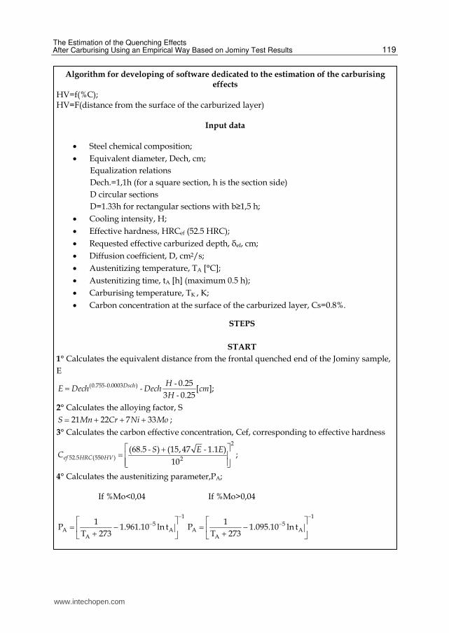
Algorithm for developing of software dedicated to the estimation of the carburising effects

HV=f(%C); HV=F(distance from the surface of the carburized layer)

Input data

Steel chemical composition;

Equivalent diameter, Dech, cm;

Equalization relations

Dech.=1,1h (for a square section, h is the section side)

D circular sections

D=1.33h for rectangular sections with b≥1,5 h;

Cooling intensity, H;

Effective hardness, HRCef (52.5 HRC);

Requested effective carburized depth, δef, cm;

Diffusion coefficient, D, cm2/s;

Austenitizing temperature, TA [°C];

Austenitizing time, tA [h] (maximum 0.5 h);

Carburising temperature, TK , K;

Carbon concentration at the surface of the carburized layer, Cs=0.8%.

STEPS

START

1° Calculates the equivalent distance from the frontal quenched end of the Jominy sample,

E

- --

-

Dsch HE Dech Dech cm

H(0.755 0.0003 ) 0.25

[ ];3 0.25

2° Calculates the alloying factor, S

S Mn Cr Ni Mo21 22 7 33 ;

3° Calculates the carbon effective concentration, Cef, corresponding to effective hardness

- -ef HRC HV

S E EC

2

52.5 (550 ) 2

(68.5 ) (15,47 1.1 );

10

4° Calculates the austenitizing parameter,PA;

If %Mo<0,04 If %Mo>0,04

1

5A A

A

1P 1.961.10 ln t

T 273

1

5A A

A

1P 1.095.10 ln t

T 273

www.intechopen.com


120

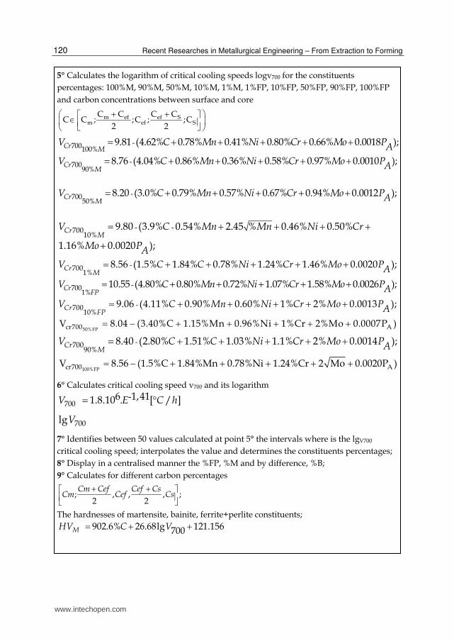
5° Calculates the logarithm of critical cooling speeds logv700 for the constituents

percentages: 100%M, 90%M, 50%M, 10%M, 1%M, 1%FP, 10%FP, 50%FP, 90%FP, 100%FP

and carbon concentrations between surface and core

m ef ef Sm ef S

C C C CC C ; ;C ; ;C

2 2

-Cr MV C Mn Ni Cr Mo PA700100%

9.81 (4.62% 0.78% 0.41% 0.80% 0.66% 0.0018 ); -Cr

MV C Mn Ni Cr Mo PA700

90%8.76 (4.04% 0.86% 0.36% 0.58% 0.97% 0.0010 );

-CrM

V C Mn Ni Cr Mo PA70050%

8.20 (3.0% 0.79% 0.57% 0.67% 0.94% 0.0012 );

- -CrM

V C Mn Mn Ni Cr

Mo PA

70010%

9.80 (3.9% 0.54% 2.45 % 0.46% 0.50%

1.16% 0.0020 );

-CrM

V C C Ni Cr Mo PA7001%

8.56 (1.5% 1.84% 0.78% 1.24% 1.46% 0.0020 ); -Cr

FPV C Mn Ni Cr Mo PA700

1%10.55 (4.80% 0.80% 0.72% 1.07% 1.58% 0.0026 );

-CrFP

V C Mn Ni Cr Mo PA70010%

9.06 (4.11% 0.90% 0.60% 1% 2% 0.0013 ); 50%FPcr700 AV 8.04 (3.40%C 1.15%Mn 0.96%Ni 1%Cr 2%Mo 0.0007P )

-CrM

V C C Ni Cr Mo PA70090%

8.40 (2.80% 1.51% 1.03% 1.1% 2% 0.0014 ); 100%FPcr700 AV 8.56 (1.5%C 1.84%Mn 0.78%Ni 1.24%Cr 2 Mo 0.0020P )

6° Calculates critical cooling speed v700 and its logarithm

-V E C h7006 1,411.8.10 . [ / ]

V700lg

7° Identifies between 50 values calculated at point 5° the intervals where is the lgV700

critical cooling speed; interpolates the value and determines the constituents percentages;

8° Display in a centralised manner the %FP, %M and by difference, %B;

9° Calculates for different carbon percentages

Cm Cef Cef CsCm Cef Cs; , , , ;

2 2

The hardnesses of martensite, bainite, ferrite+perlite constituents;

MHV C V902.6% 26.68lg 121.156700

www.intechopen.com


121

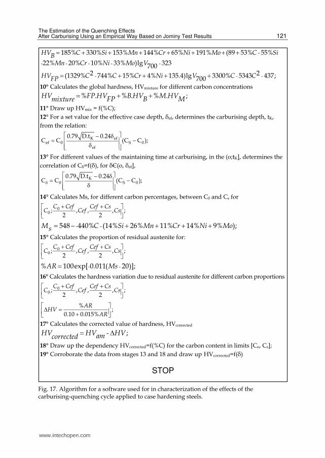
Fig. 17. Algorithm for a software used for in characterization of the effects of the carburising-quenching cycle applied to case hardening steels.

- - - - -

- - -

-

HV C Si Mn Cr Ni Mo C SiBMn Cr Ni Mo V

HV C C Cr Ni V C CFP

185% 330% 153% 144% 65% 191% (89 53% 55%

22% 20% 10% 33% )lg 3237002 2(1329% 744% 15% 4% 135.4)lg 3300% 5343 437;700

10° Calculates the global hardness, HVmixture for different carbon concentrations

HV FP HV B HV M HVFP B Mmixture % . % . % . ;

11° Draw up HVmix = f(%C);

12° For a set value for the effective case depth, δef, determines the carburising depth, tK,

from the relation:

K efef 0 S 0

ef

0.79 D.t 0.24C C (C C );

13° For different values of the maintaining time at carburising, in the (o;tK], determines the

correlation of Cδ=f(δ), for δЄ(o, δef],

K0 S 0

0.79 D.t 0.24C C (C C );

14° Calculates Ms, for different carbon percentages, between C0 and Cs for

C Cef Cef CsC Cef Cs0

0 ; , , , ;2 2

- -M C Si Mn Cr Ni Mos 548 440% (14% 26% 11% 14% 9% );

15° Calculates the proportion of residual austenite for:


0 ; , , , ;2 2

- -AR Ms% 100exp[ 0.011( 20)];

16° Calculates the hardness variation due to residual austenite for different carbon proportions


0 ; , , , ;2 2

ARHV

AR

%;

0.10 0.015%

17° Calculates the corrected value of hardness, HVcorrected

- HV HV HVamcorrected ;

18° Draw up the dependency HVcorrected=f(%C) for the carbon content in limits [Co, Cs];

19° Corroborate the data from stages 13 and 18 and draw up HVcorrected=f(δ)

STOP

www.intechopen.com


122

6. References

[1] Murry, G. (1971). Mem.Scient.Rev.Met, no.12,pp.816-827 [2] Bussmann, A. (1999). Definition des mathem.Modells,CET [3] Jatczak, C. F. (1971). Determining Hardenability from Composition. Metal Progress,

vol.100, no.3, pp.60-65 [4] Wyss, U. (1988) Kohlenstoff und Härteverlauf in der Einsatzhärtungsschicht verschieden

legierter Einsatzstähle, Härt.Tech.Mitt., no.43,1 [5] Popescu, N., Cojocaru, M. (2005). Cementarea oţelurilor prin instilarea lichidelor

organice. Ed.Fair Partners, pp.115, Bucuresti [6] Just, E. (1986). Formules de trempabilité. Härt.Tech.Mitt., no.23, pp.85-100 [7] Roempler, D., Weissohn, K. H. (1989). Kohlenstoff und Härteverlauf in der

Einsatzhärtungsschicht-Zusatzmodul für Diffusionrechner, AWT-Tagung, Einsatzhärten, Darmstadt

[8] Maynier, Ph., Dollet, J., Bastien, P. (1978). Hardenability Concepts with Applications to Steel, AIME, pp.163-167, 518-545

[9] Carsi, M., de Andrés, M.P. (1990). Prediction of Melt-Hardenability from Composition. Symposium IFHT,Varşovia

[10] Eckstein, H.J. (1987). Technologie der Wärmebehandlung von Stahl. VEB Deutscher Verlag für Grundstoffindustrie,Leipzig

www.intechopen.com

Recent Researches in Metallurgical Engineering - From Extractionto FormingEdited by Dr Mohammad Nusheh

ISBN 978-953-51-0356-1Hard cover, 186 pagesPublisher InTechPublished online 23, March, 2012Published in print edition March, 2012

InTech EuropeUniversity Campus STeP Ri Slavka Krautzeka 83/A 51000 Rijeka, Croatia Phone: +385 (51) 770 447 Fax: +385 (51) 686 166www.intechopen.com

InTech ChinaUnit 405, Office Block, Hotel Equatorial Shanghai No.65, Yan An Road (West), Shanghai, 200040, China

Phone: +86-21-62489820 Fax: +86-21-62489821

Metallurgical Engineering is the science and technology of producing, processing and giving proper shape tometals and alloys and other Engineering Materials having desired properties through economically viableprocess. Metallurgical Engineering has played a crucial role in the development of human civilization beginningwith bronze-age some 3000 years ago when tools and weapons were mostly produced from the metals andalloys. This science has matured over millennia and still plays crucial role by supplying materials havingsuitable properties. As the title, "Recent Researches in Metallurgical Engineering, From Extraction to Forming"implies, this text blends new theories with practices covering a broad field that deals with all sorts of metal-related areas including mineral processing, extractive metallurgy, heat treatment and casting.

How to referenceIn order to correctly reference this scholarly work, feel free to copy and paste the following:

Mihai Ovidiu Cojocaru, Niculae Popescu and Leontin Drugă (2012). The Estimation of the Quenching EffectsAfter Carburising Using an Empirical Way Based on Jominy Test Results, Recent Researches in MetallurgicalEngineering - From Extraction to Forming, Dr Mohammad Nusheh (Ed.), ISBN: 978-953-51-0356-1, InTech,Available from: http://www.intechopen.com/books/recent-researches-in-metallurgical-engineering-from-extraction-to-forming/the-estimation-of-the-quenching-effects-after-carburising-in-an-empirical-way-using-the-jominy-test-

© 2012 The Author(s). Licensee IntechOpen. This is an open access articledistributed under the terms of the Creative Commons Attribution 3.0License, which permits unrestricted use, distribution, and reproduction inany medium, provided the original work is properly cited.

http://creativecommons.org/licenses/by/3.0

Documents

The Estimation of the Quenching Effects After Carburising ...cdn.intechopen.com/pdfs/32752/InTech-The... · The Estimation of the Quenching Effects After Carburising Using an Empirical